RICE PRICES AND INCOME DISTRIBUTION IN …deaton/downloads/Rice_Prices...The Economic Journal, 99 (Conference I 989), 1-37 Printed in Great Britain RICE PRICES AND INCOME DISTRIBUTION

The Economic Journal, 99 (Conference I 989), 1-37

Printed in Great Britain

RICE PRICES AND INCOME DISTRIBUTION IN THAILAND: A NON-PARAMETRIC ANALYSIS*

Angus Deaton

In the postwar period, the government of Thailand has exercised a range of policy instruments that have influenced the prices of agricultural goods. Policies towards the export of rice have been the most important, but a range of other goods, specifically sugar, rubber, maize, and vegetable oils has also been directly subject to government policy. The history and political economy of these policies have recently been well described by Siamwalla and Setboonsarng (i987), who also make estimates of the economic effects on domestic prices, on transfers of resources between agriculture and government, and on consumer welfare. In an earlier study of rice policies, Trairatvorakul (I984) makes an even more ambitious attempt to track the effects of the policies, not only on government revenue and household welfare, but also as far as the influences on urban and rural real wages, and on the nutritional status of the population.

This paper is less ambitious than either of these earlier studies, and focuses on only one part of the story, albeit a part that is important and that has been lightly researched in the earlier literature. I am concerned here with patterns of household demand and supply and how knowledge of those patterns affects the assessment of pricing policies. I have two main aims, one substantive, and one methodological.

My first, substantive, aim is to examine the effects of rice prices on the distribution of real incomes across different households. I do this by describing consumption and production patterns for rice in relation to household characteristics, particularly living standards and geographical location. Such description is important because it provides an easily comprehended 'map' of the immediate effects of price changes, and although such maps contain a good deal less than everything that we should like to know, they are based on good data, and provide perhaps the only firm information we possess about the effects of changes in pricing policy. Using a household survey, the i98I-2

Socioeconomic Survey of the Whole Kingdom, I find that higher rice prices can be expected to provide direct benefits to rural households at all levels of living, but that the main beneficiaries are neither the poorest rural households nor, more surprisingly, the richest rural households. The immediate effect of higher rice

* Frank Paish Memorial Lecture. The research behind the results reported here was funded in part by the Asian Development Bank and by a grant from the McDonnell Foundation to the Center for International Studies. I thank Ammar Siamwalla and other staff members of the Thai Development Research Institute for their help and cooperation. Grateful acknowledgement for comments is made to Jere Behrman, Henry Bienen, Anne Case, Mark Gersovitz, Terence Gorman, Georgejakubsen, John Lewis, and Christina Paxson. Isaac Lee provided computational assistance. The paper is based on RPDS Working Paper No. I36, 'Agricultural pricing policies and demand patterns in Thailand,' February and March, I988.

I [ I ] ECS 99

2 THE ECONOMIC JOURNAL [CONFERENCE

prices is to redistribute income towards households in the middle of the rural income distribution.

My second, methodological, aim is to explore statistical methods that do justice to the richness of the household survey data, and that allow convincing demonstration and presentation of results with a minimum of unnecessary assumption. Economists who typically analyse time series data, containing a hundred or so observations, have the luxury of being able to examine and present their data, for example by graphing the series as a function of time. For cross-sectional survey data, with many thousands of observations, it is less obvious what are the appropriate graphical tools. Histograms are frequently useful for single variables, but the relationship between variables is harder to describe. Even in two dimensions but with, say, ten thousand observations, the (computer-generated) scatter diagram is typically too 'messy' to be informative. Instead heavy reliance is placed on cross-tabulations and on linear regressions as means of summarising the data. The former are not very flexible and do not transmit information clearly, while the latter tend to over- summarise, rarely doing justice to the amount of information available. In the analysis below, I shall make heavy use of simple non-parametric techniques for regression and density estimation. These methods, although not without problems of their own, provide easily comprehended graphical descriptions of the data that are directly informative about the problem at hand. And although everything that I shall present could have been derived by an alternative, more familiar econometric analysis, I shall argue that, in practice, it would have been a good deal more difficult to do so. Moreover, since the techniques call for little more than presentation of the data, relying minimally on auxiliary economic or econometric assumptions, I hope that the results, although limited in scope, will compensate by being unusually convincing.

The plan of the paper is as follows. The organisation follows the substantive question of rice pricing with methodological comments along the way. Section I provides a brief theoretical outline that motivates the empirical work. Section II presents the analysis of demand and supply patterns for rice and of the distributional consequences of alternative pricing schemes. Section III concludes.

I. DEMAND PATTERNS AND PRICING POLICY

Changes in an export tax like the Thai rice 'premium' will generally have widespread and complex effects throughout the economy. The most immediate and obvious are the effects on government revenue and on household and farmer real incomes. For the latter, consider a farm or non-farm household that consumes rice, may or may not produce rice, and trades in other commodities and in the labour market. A simple representation of household living standards is given by the indirect utility function.

Uh = f(WT+b+a, p), (I)

where uh is utility (or real income) of household h, w is the wage rate, T is the total time available, b is rental income, property income, or transfers, p is a

I989] RICE DISTRIBUTION IN THAILAND 3

price vector of commodities consumed, and iT is the household's profits from farming or other family business. Since profits are maximised, we can think of iT as the value of a profit function, ir(p, v, w), say, where v is a price vector of input prices, w is the wage rate, or vector of household wages, and p in this context is the vector of output prices for commodities, such as agricultural goods, that are produced by the household. A standard property of the profit function is that

air/api = yi, (2)

where yi is the (gross) production of good i by the household (or farm). Given these functions, the effects of price changes on household real income

are straightforward to derive. In particular, we have

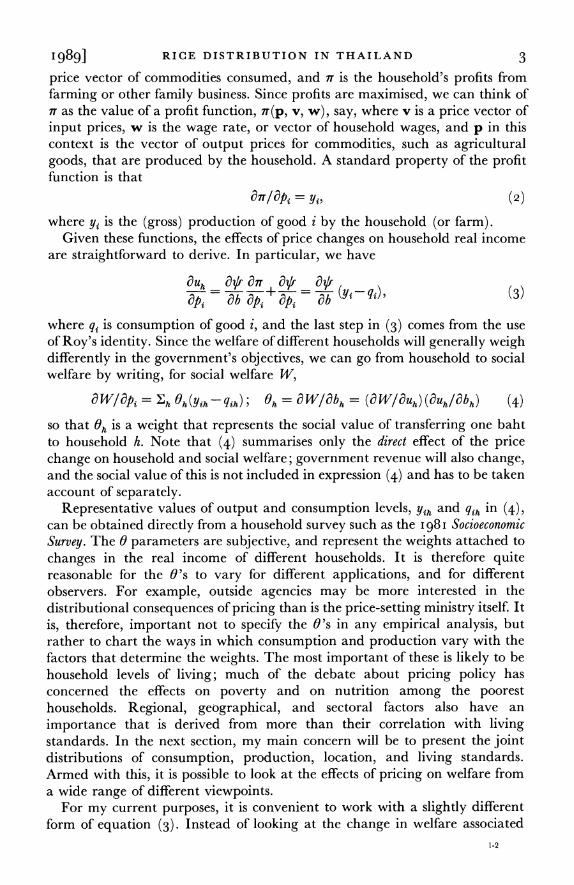
aUh - 0y r+ 0' =_ y_ - i)) ap, ab ap, ap, - b

where qi is consumption of good i, and the last step in (3) comes from the use of Roy's identity. Since the welfare of different households will generally weigh differently in the government's objectives, we can go from household to social welfare by writing, for social welfare W,

a W/aPi = lh Oh (Yih - qih); h = a W/abh = (a W/Uh) (aUh/abh) (4)

so that Oh is a weight that represents the social value of transferring one baht to household h. Note that (4) summarises only the direct effect of the price change on household and social welfare; government revenue will also change, and the social value of this is not included in expression (4) and has to be taken account of separately.

Representative values of output and consumption levels, Yih and qih in (4), can be obtained directly from a household survey such as the I98 I Socioeconomic Survey. The 6 parameters are subjective, and represent the weights attached to changes in the real income of different households. It is therefore quite reasonable for the 6O's to vary for different applications, and for different observers. For example, outside agencies may be more interested in the distributional consequences of pricing than is the price-setting ministry itself. It is, therefore, important not to specify the 6O's in any empirical analysis, but rather to chart the ways in which consumption and production vary with the factors that determine the weights. The most important of these is likely to be household levels of living; much of the debate about pricing policy has concerned the effects on poverty and on nutrition among the poorest households. Regional, geographical, and sectoral factors also have an importance that is derived from more than their correlation with living standards. In the next section, my main concern will be to present the joint distributions of consumption, production, location, and living standards. Armed with this, it is possible to look at the effects of pricing on welfare from a wide range of different viewpoints.

For my current purposes, it is convenient to work with a slightly different form of equation (3). Instead of looking at the change in welfare associated

1-2


with a price change, we can ask how much money (positive or negative) the household would require in order to maintain its previous level of living. If the price change is dpi, and the required compensation is dB, then, from (3),

dB = (qi-yi) dp- =pi(qi -y) dlnpi (5)

so that, if dB is expressed as a fraction of household expenditure x, we have

(dB/x) = (wi -pi yi/x) d ln pi, (6)

where wi = pi qi/x is the budget share of good i, and pi yi/x is the value of production of i as a fraction (or multiple) of total household expenditure. Equation (6) is particularly convenient for empirical analysis since wi -pi yJ/ x, which I shall call the net consumption ratio, is the elasticity of the cost of living with respect to the price of good i. For net producers of the good, the elasticity will be negative, and for net consumers positive. Further, the relationship between the net consumption ratio and any household characteristic determines the distributional effects of the price change with respect to that characteristic. For example, if the ratio is distributed independently of household living standards, or if it is the same on average in two different regions, then price changes will not affect the real distribution of income, or the distribution between the two regions. For this reason, it is the net consumption ratio that will be documented in the next section.

The proportional or elasticity formulation in (6) is also convenient because it automatically takes care of the fact that farmers produce, not rice, but paddy, while consumers consume rice. Suppose that there is a fixed rice yield, A < i,

say, from each kilogram of paddy, so that if the price of rice is pi, the price of paddy is Api. Farmers' profits depend on Api, while consumer costs depend directly on pi. If pi changes, with the paddy price moving proportionately, the compensation dB in (5) is now (qi - Ayi) dpi, since the producer benefit is proportional, not to yi but to Ayi. As before, we can use the fact that dpi = Pi d ln pi to write dB as pi(qi - Ayi) d ln pi, which, since Api yi is just the value of sales of paddy, is purchases of rice less sales of paddy multiplied by d ln pi. In consequence, equation (6) is correct, provided that pi yi is interpreted as the value of production.

For some purposes, it is useful to keep separate the production and consumption terms in (3) and (6). In the Thai context, sugar farmers would be an example. Farmers produce sugar cane, and sell it to the mills at one price, and they buy refined sugar at a different price. Given the complexities of Thai sugar policy, the two prices may not even move together. In these circumstances, it makes sense to consider production and consumption as disjoint activities, and to look at the separate effects of price changes on income generation on the one hand, and on the cost of living on the other. By contrast, for a subsistence paddy farmer who consumes much or all of what he produces, it would rarely be useful to make the distinction between the two effects.


II. DEMAND AND SUPPLY PATTERNS FOR RICE IN THAILAND

IN I 981/2

In this section, I use data from the I 981/2 Socioeconomic Survey to describe patterns of demand and supply for rice. I shall be particularly concerned with how supply, demand, and living standards are related to one another, and how the relationships vary geographically. I begin with a brief description of the relevant parts of the household survey. It is from this that all the Tables and Charts in the report are constructed.

Table I shows the numbers of survey households and their distribution over the kingdom. There are I I,893 survey households used in this study; they are distributed as shown over the three sectors, municipal areas (urban), sanitary districts (semi-urban), and villages (rural). The survey is designed to give each household an equal probability of inclusion within each of the sectors, but not between them. Households in municipal areas are less expensive to sample and are over-represented while those in villages are correspondingly under- represented. In order to avoid having to make weighting corrections, and because the sectoral division is itself inherently interesting, I shall keep the three sectors separate throughout the analysis. There are five standard regions, North, North-East, Centre, South, and Bangkok, all of which are represented in each of the sectors. These can be further divided into the twelve regions shown in Table i, all of which, apart from the centre of Bangkok, have some

Table I

Structure of the Sample

Community types

Municipal areas Sanitary districts Villages

hh am blx hh am blx hh am blx Regions

North Upper 313 4 27 326 13 38 598 17 99 North Lower 259 6 23 137 I I 22 628 i9 io6

North East Upper 272 3 24 310 13 40 1,015 17 I69

North East Lower 303 4 27 243 13 32 977 20 I63

Central West 120 3 II I67 7 21 293 9 49 Central Middle 172 6 15 280 I I 37 547 12 93 Central East 141 5 13 31 4 4 321 10 54 South Upper 393 10 34 147 7 I9 494 2 1 83

South Lower 207 4 i8 22 3 3 146 8 25

Bangkok Central 1,533 8 136 0 0 0 0 0 0

Bangkok Suburbs 403 3 36 172 I 22 ii6 I I9

Bangkok Fringe 43 I 4 63 I 8 701 4 ii8

Totals 4,159 57 368 I,898 84 246 5,836 138 978

hh = households, am = amphoes, blx = blocks or villages. Block sizes are designed to have 12 households in municipal areas, 8 households in sanitary districts, and

6 households in villages. Source: I981-2 Socioeconomic Survey, author's calculations.


households in each sector of the survey. I shall use both the broad and fine regional breakdown; for rice in particular, cropping and consumption patterns of glutinous versus non-glutinous rice are quite different in the two parts of each of the North and North East regions.

Table i also shows the numbers of amphoes and blocks in each of the subregions. The amphoes are regions rather smaller than the seventy or so provinces of the country, and were chosen, not at random, but to match the amphoes in the previous (I 975-6) socioeconomic survey. Within each amphoe, a number of blocks were randomly selected, the number being such as to ensure that, with a fixed block size, each household had an equal probability of selection. The design was for I 2 households per block in municipal areas, 8 in sanitary districts, and 6 in villages; in practice there are minor deviations from the intent.

Table 2 presents sample means for the main variables of interest. Throughout this study, I use total household expenditure per head (xpc) as my preferred measure of household living standards; it is measured here as total household expenditure on non-durables per month divided by the number of persons in the household. Judging by this criterion, and ignoring any price differences, households in municipal areas have higher living standards than those in sanitary districts, who in turn are better off than village households. There are very marked regional disparities in these means. The average xpc of households in Municipal Areas is more than twice the average xpc in village households, while the discrepancy between an average urban household in Bangkok and an average village household in the North East is closer to four to one. Overall, northern and particularly north-eastern rural households are the poorest, with central and southern areas in the middle of the distribution, and Bangkok at the top. I shall return to the distributions within these averages below. Note also that urban households tend to be headed by somewhat younger people, and that rural household sizes are larger. Again, the North East is the outlier; household sizes are on average a full person larger than in municipal areas as a whole.

The second panel of Table 2 shows the regional distribution of the rice crops. Note that while I have converted the annual production values to a monthly basis, the figures are given on a household and not on an individual basis and therefore should not be compared with the values of xpc in the first panel. Although there is a good deal of production by sanitary district and municipal area households, I shall focus on the much more important rural population in the third part of the table.

On average, village households produced 9IO baht worth of rice (glutinous or non-glutinous) per month, a figure that is about thirty per cent of average household expenditure on all goods, and more than twice the value of their total consumption of rice. Clearly, rice pricing policy is capable of transferring very significant resources in and out of the sector as a whole. The major rice producing regions are the (very wide) rural Fringe Area around Bangkok, the Lower North and the Centre, with the Lower North East also important. At any specific location, production is either rice or glutinous rice, with


Table 2

Summary Data

All N Up N Lw NE Up NE Lw Centre South B'kok

Characteristics Municipal areas Family size 4-1 3-6 39 44 4.I 4.1 4.1 4-2

Head's age 422 44 7 41.7 42-0 395 450 41.8 418

Exp. per head 1,5I6 1,394 1,562 1,171 1,172 1,497 1,36I i,68o

Production value Rice 17 0 130 0 9 33 I8 4

Glutinous rice 3 26 4 4 3 0 0 0

Expenditures Rice 208 I46 251 I25 I89 244 227 2I3

Glutinous rice 35 I80 10 173 87 3 7 3

Budget shares Rice 451 3.05 &70 282 482 5.66 589 397

Glutinous rice iso8 5 75 033 5.36 2-86 oo6 0-I7 o-o8

Sanitary districts Characteristics

Family size 4-2 39 4-2 49 44 42 39 4-0

Head's age 45I 43 8 454 435 44'2 49'2 48-1 39'2

Exp. per head 902 779 754 710 767 993 1,002 1,292

Production value Rice 308 77 949 48 239 69I 105 34

Glutinous rice 124 296 25 350 107 0 0 0

Expenditures Rice I99 3I 289 52 24I 318 235 265

Glutinous rice 142 338 II 400 104 6 20 8

Budget shares Rice 6-88 0o98 12-35 i 66 9199 1101 8&47 6.03

Glutinous rice 6-5I i6-73 048 i6-88 5.68 O-I8 055 0'20

Villages Characteristics

Family size 46 4-1 43 52 5-1 43 45 44 Head's age 45 4 440 43.6 44 1 449 48-I 45 7 46.o

Exp. per head 675 56o 647 472 44I 862 712 1021

Production value Rice 732 56 I,384 48 502 1,I75 362 1,514

Glutinous rice 177 370 87 532 209 8 4 I

Expenditures Rice 233 20 337 15 292 360 303 277

Glutinous rice 155 357 40 454 176 I4 2 1 8

Budget shares Rice 10.39 I-08 17-38 o69 I7.14 13'77 I3-68 8-41

Glutinous rice 8.31 2o069 2-o6 2395 9-64 044 070 O-I8

Notes: Expenditure per head (xpc) is total household expenditure (in baht) on non-durable goods per month divided by the number of persons in the household. Married children living with their parents are treated as separate households, even if they share the same food and kitchen. Production values are one twelfth of the annual value of crops; the mean is taken over all households whether or not they produce anything. Expenditures are also baht per month per household (not per person). Budget shares are percentages of total household expenditure on non-durables.

N Up and N Lw are Upper and Lower North, similarly for NE Up and NE Lw; B'kok is Bangkok. Source: 1981-2 Socioeconomic Survey, author's calculations.


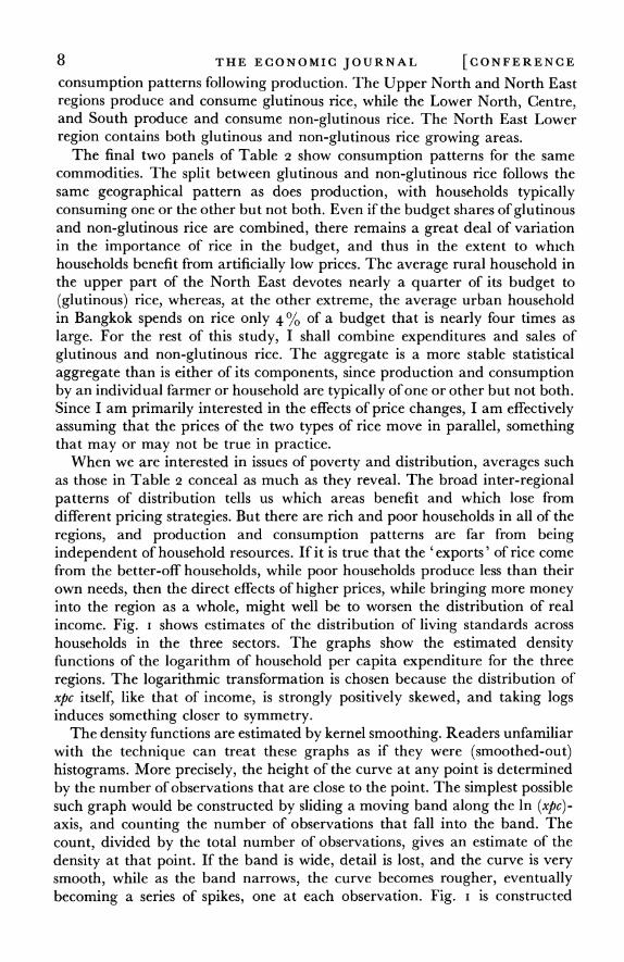
consumption patterns following production. The Upper North and North East regions produce and consume glutinous rice, while the Lower North, Centre, and South produce and consume non-glutinous rice. The North East Lower region contains both glutinous and non-glutinous rice growing areas.

The final two panels of Table 2 show consumption patterns for the same commodities. The split between glutinous and non-glutinous rice follows the same geographical pattern as does production, with households typically consuming one or the other but not both. Even if the budget shares of glutinous and non-glutinous rice are combined, there remains a great deal of variation in the importance of rice in the budget, and thus in the extent to which households benefit from artificially low prices. The average rural household in the upper part of the North East devotes nearly a quarter of its budget to (glutinous) rice, whereas, at the other extreme, the average urban household in Bangkok spends on rice only 4 % of a budget that is nearly four times as large. For the rest of this study, I shall combine expenditures and sales of glutinous and non-glutinous rice. The aggregate is a more stable statistical aggregate than is either of its components, since production and consumption by an individual farmer or household are typically of one or other but not both. Since I am primarily interested in the effects of price changes, I am effectively assuming that the prices of the two types of rice move in parallel, something that may or may not be true in practice.

When we are interested in issues of poverty and distribution, averages such as those in Table 2 conceal as much as they reveal. The broad inter-regional patterns of distribution tells us which areas benefit and which lose from different pricing strategies. But there are rich and poor households in all of the regions, and production and consumption patterns are far from being independent of household resources. If it is true that the 'exports' of rice come from the better-off households, while poor households produce less than their own needs, then the direct effects of higher prices, while bringing more money into the region as a whole, might well be to worsen the distribution of real income. Fig. I shows estimates of the distribution of living standards across households in the three sectors. The graphs show the estimated density functions of the logarithm of household per capita expenditure for the three regions. The logarithmic transformation is chosen because the distribution of xpc itself, like that of income, is strongly positively skewed, and taking logs induces something closer to symmetry.

The density functions are estimated by kernel smoothing. Readers unfamiliar with the technique can treat these graphs as if they were (smoothed-out) histograms. More precisely, the height of the curve at any point is determined by the number of observations that are close to the point. The simplest possible such graph would be constructed by sliding a moving band along the In (xpc)- axis, and counting the number of observations that fall into the band. The count, divided by the total number of observations, gives an estimate of the density at that point. If the band is wide, detail is lost, and the curve is very smooth, while as the band narrows, the curve becomes rougher, eventually becoming a series of spikes, one at each observation. Fig. i is constructed

1989] RICE DISTRIBUTION IN THAILAND 9

075 r

0*60 Villages

Municipal areas;

4 0.45 Sanitary districts

:O*3O

?; I/

0-00

4.0 5.0 6.0 7-0 8.0 9.0

In (xpc): In (baht)

Fig. i. Sectoral distributions.

according to this 'moving band' principle, but with the complication that observations that are close to the point where the density is being constructed, i.e. those at the centre of the band, are given greater weight than observations far from the centre. Provided that the width of the band is allowed to tend to zero as the sample size increases, the resulting graph will consistently estimate the true density. The formal details of the procedures are confined to the Appendix.

The most obvious feature of Fig. I is the relative positions of the three sectors: the modal urban household is very well off indeed by village standards. Perhaps less obvious is the size of the disparities. A difference of 2 on a logarithmic scale corresponds to scale factor of 7-4 and a difference of I to a scale factor of 2-7. The distribution in the villages, even after the logarithmic transformation, has a long upper tail; there are very rich households in the rural areas in spite of the very low mode.

Rice shares at each point of these distributions are estimated and plotted in Fig. 2. The graphs shown are non-parametric regressions of the rice share on the logarithm of household per capita expenditure, estimated, once again, by kernel smoothing. At any given value of ln (xpc), what is shown is a weighted average of the values of the rice share for observations nearby, i.e. those within the kernel. The weights are the same weights used to construct the density (points nearby get higher weight), but are scaled by the estimate of the density at-the point. Hence, as the sample size gets larger, the estimate will converge on the conditional expectation of the rice share given the value of total expenditure. Once again, a more formal treatment is given in the Appendix. While plots of estimated regressions would look rather similar, the advantage of the technique used here is that the data are allowed to choose the shape of

IO THE ECONOMIC JOURNAL [CONFERENCE

36.0,.

29-0 -

; 22.0 -

15.1a

8.1 . ......... Villages - - Sanitary districts.

- Municipal areas

5.0 5.7 6.4 7 1 7.8 8.5 In (xpc): In (bafit)

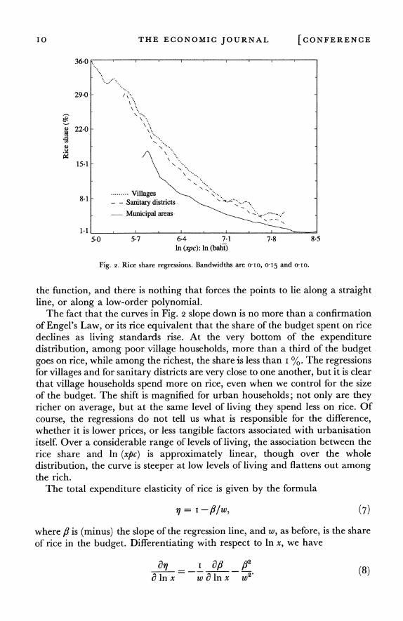
Fig. 2. Rice share regressions. Bandwidths are O-IO, 0-I5 and o'Io.

the function, and there is nothing that forces the points to lie along a straight line, or along a low-order polynomial.

The fact that the curves in Fig. 2 slope down is no more than a confirmation of Engel's Law, or its rice equivalent that the share of the budget spent on rice declines as living standards rise. At the very bottom of the expenditure distribution, among poor village households, more than a third of the budget goes on rice, while among the richest, the share is less than i %. The regressions for villages and for sanitary districts are very close to one another, but it is clear that village households spend more on rice, even when we control for the size of the budget. The shift is magnified for urban households; not only are they richer on average, but at the same level of living they spend less on rice. Of course, the regressions do not tell us what is responsible for the difference, whether it is lower prices, or less tangible factors associated with urbanisation itself. Over a considerable range of levels of living, the association between the rice share and ln (xpc) is approximately linear, though over the whole distribution, the curve is steeper at low levels of living and flattens out among the rich.

The total expenditure elasticity of rice is given by the formula

y = I-/J/w, (7)

where ,? is (minus) the slope of the regression line, and w, as before, is the share of rice in the budget. Differentiating with respect to ln x, we have

____ __ _ If@2 (8)

I989] RICE DISTRIBUTION IN THAILAND II

By inspection of the graph, the first term on the right hand side is positive, while the second must be negative; for the values shown here, the second term dominates, and we have the traditional result that the expenditure elasticity is lower for better-off households. For the data in Fig. 2, the total expenditure elasticity falls from o 5 or so for the poorest households to approximately zero at the top of the distribution.

Budget share Engel curves such as those in Fig. 2 describe the average welfare effects of price changes that operate through consumption. If all farmers were to continue to receive the same price for production, but the consumer price were to increase by io%, the poorest households would suffer a 3-6 % fall in living standards and the richest only o- i %. These figures could be rather different if the possible response of the budget shares to the price change were taken into account, but there is no reason to suppose that the response would vary much by level of living, so that the distributional consequences of the price change would not be much affected. Apart from the obvious omission of the production side, which I shall deal with next, the curves in Fig. 2 can also be faulted for giving no impression of the variability in consumption patterns at each level of xpc. On average, poor consumers spend a third of their budgets on rice, but the effects of pricing policy on poverty depend on whether such an average is typical, or whether there are significant numbers of poor households that spend much more. At the other end of the distribution, significant numbers of rich households with large rice budgets will generate a powerful lobby for low prices.

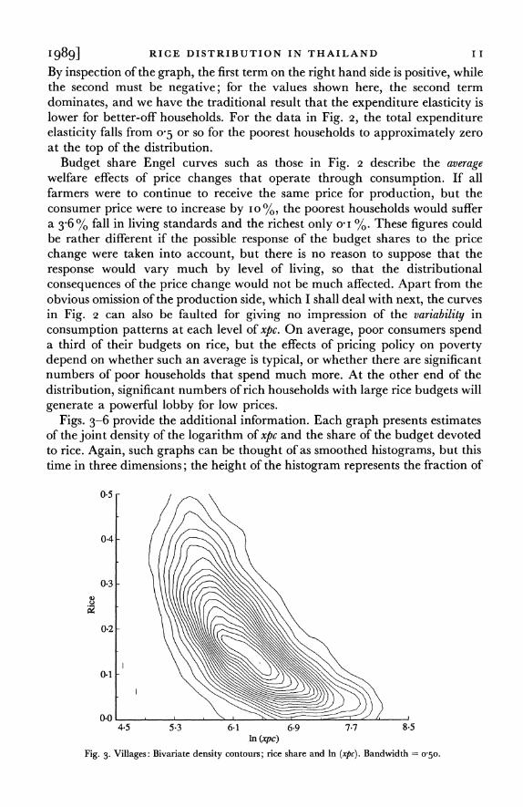
Figs. 3-6 provide the additional information. Each graph presents estimates of the joint density of the logarithm of xpc and the share of the budget devoted to rice. Again, such graphs can be thought of as smoothed histograms, but this time in three dimensions; the height of the histogram represents the fraction of

0.5 -

0 3-

0.2-

0.1

0.0 4-5 5.3 6-1 6 9 7-7 8.5

In (xpc)

Fig. 3. Villages: Bivariate density contours; rice share and In (xpc). Bandwidth = o 50.

I2 THE ECONOMIC JOURNAL [CONFERENCE

0.5

0.4 -

0.3 -

0.2 - _

0.1 j

4-5 5.4 6.3 7-2 8-1 9.0 In (xpc)

Fig. 4. Sanitary districts: Bivariate density contours; rice share and In (xpc). Bandwidth = 05.

0.40

0-32

0-24

0.16

0.08

0*00 5-0 5-8 6-6 7.4 8-2 9*0

In (xpc)

Fig. 5. Municipal areas: Bivariate density contours; rice share and In (xpc). Bandwidth = o5O.

households at the levels of xpc and rice share represented by the co-ordinates along the base. The technique is much the same as before, although now observations are counted and weighted, not in an interval band around each point, but in a two dimensional elliptical band; the details are in the Appendix. Figs. 3-5 are contour maps; points linked by a contour have the same density, and the contours are equally spaced. Fig. 6, which is a different representation of the same data given in Fig. 5, gives a visual impression of the surface of the

I989] RICE DISTRIBUTION IN THAILAND I3

7.5

6-0

4-5

3*0

1-5

Rice 0101 In (xpc)

Fig. 6. Municipal areas: Joint density surface.

joint density; although such graphics conceal some of the information given in the contour plots, they give a clearer impression of relative heights and thus of the concentration of mass. In addition, the visual impact of the contour plots is often dominated by information about the tails of the distribution where there may be very few observations.

These diagrams fill out the skeletal information in the regression functions in Fig. 2. The contour plot for the villages shows greater diversity in rice budgeting patterns, a diversity which is greater the poorer are the households concerned. For example, for households with ln (xpc) around 5-3, that is with 200 baht per head per month, the mean rice share is close to a third, see Fig. 2 or Fig. 3, but there is an enormous range of behaviour; there are households with shares of i 0 % and those with shares of 50 %. As we move towards richer households, the regression line flattens out, and the variance around it is sharply reduced. Essentially no rich households spend more than io % of their budget on rice.

Expenditure patterns are also more homogeneous in sanitary districts and municipal areas than in rural areas. In Fig. 4 the contour lines are closely bunched near the mode, and although the pattern of decreasing diversity with rising income is repeated, the whole distribution is much more concentrated than in the villages. The process of homogenisation is carried furthest in the municipal areas where the density falls away very sharply from the mode. Note also that Fig. 5 is drawn on a larger scale than either Figs. 3 or 4. There are no rich urban households who spend more than a few percent of their budget on rice. The density in the urban areas does not fall to zero as the rice share goes to zero; there are substantial numbers of urban households who record no purchases of rice. Fig. 6, with its open 'hole' or 'cave' is perhaps the best


illustration. Some of this will reflect the fact that not all households buy rice over the survey period, but more important is probably the purchase of meals rather than food by urban residents, particularly in Bangkok. Unfortunately I cannot directly allow for this, since I have no data on the proportion of pre-cooked meals that is accounted for by rice. A more detailed analysis would have to make some allowance for this in assessing the impact of food prices on urban residents.

Note finally that in all three of Figs. 3-5 there are short line segments detached from the main contours. These are genuine contour segments that result from the presence of observations that are 'outliers' with respect to the main distribution. Of course, the density is very small at such points, but they nevertheless show up because there are no other observations around them, and the width of the elliptical band is the same at all points in the graphs. From a technical point of view, it could be argued that the 'roughness' of these contour maps in the tails of the distributions indicates that the plots are undersmoothed in those areas, a problem that can be dealt with by widening the bandwidth where the density is small. However, there are advantages of undersmoothing beyond the detection of outliers. Much interest focuses on the positions of poor and rich households, and both groups are located in the tails of the distribution. Too little smoothing means that too much information is being presented, something that may be a good thing in the tails of the distribution which is where information is needed the most.

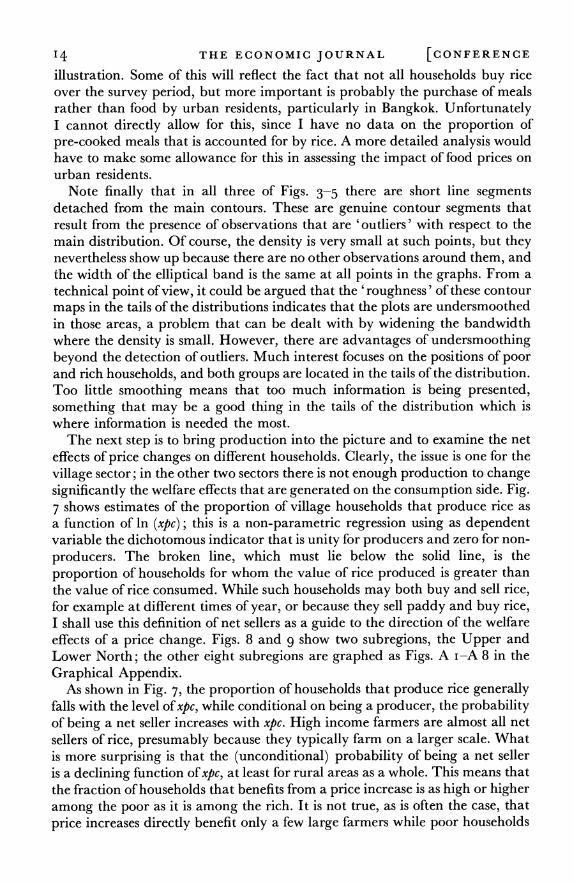
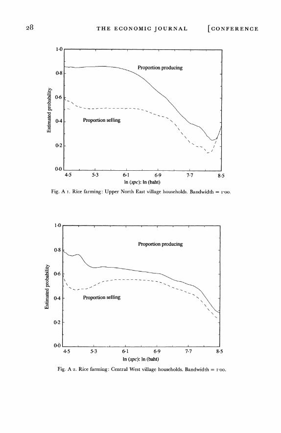
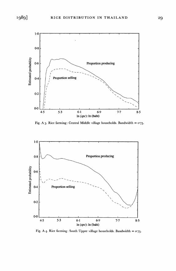
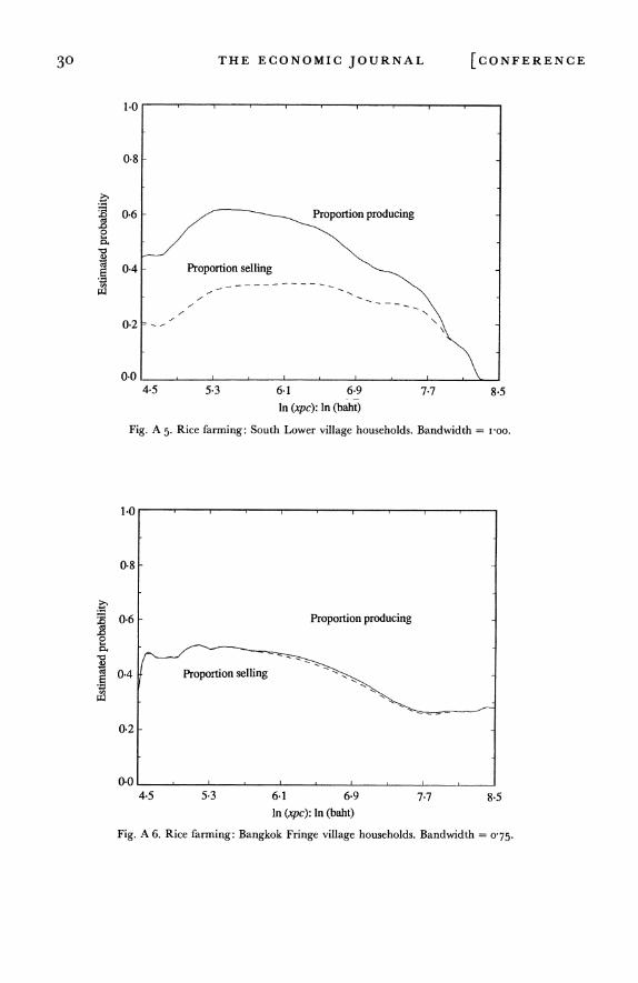
The next step is to bring production into the picture and to examine the net effects of price changes on different households. Clearly, the issue is one for the village sector; in the other two sectors there is not enough production to change significantly the welfare effects that are generated on the consumption side. Fig. 7 shows estimates of the proportion of village households that produce rice as a function of ln (xpc); this is a non-parametric regression using as dependent variable the dichotomous indicator that is unity for producers and zero for non- producers. The broken line, which must lie below the solid line, is the proportion of households for whom the value of rice produced is greater than the value of rice consumed. While such households may both buy and sell rice, for example at different times of year, or because they sell paddy and buy rice, I shall use this definition of net sellers as a guide to the direction of the welfare effects of a price change. Figs. 8 and 9 show two subregions, the Upper and Lower North; the other eight subregions are graphed as Figs. A i-A 8 in the Graphical Appendix.

As shown in Fig. 7, the proportion of households that produce rice generally falls with the level of xpc, while conditional on being a producer, the probability of being a net seller increases with xpc. High income farmers are almost all net sellers of rice, presumably because they typically farm on a larger scale. What is more surprising is that the (unconditional) probability of being a net seller is a declining function of xpc, at least for rural areas as a whole. This means that the fraction of households that benefits from a price increase is as high or higher among the poor as it is among the rich. It is not true, as is often the case, that price increases directly benefit only a few large farmers while poor households

I989] RICE DISTRIBUTION IN THAILAND I5

1 -0 ,,,,*-' -

0-8 -\

Proportion producing

i06 -

t 0-4 Proportion selling

0.2-

0-2

0.0 ,I * I , I . I

4-5 5.3 6-1 6.9 7.7 8-5

In (xpc): In (baht)

Fig. 7. Rice farming: All village households. Bandwidth = 050.


0 - -

,0-4 Proportion selling _ -

_ _ _ _-

0.6 - - -

0-2 -

0-0 4-5 5-3 6.1 6.9 7.7 8.5

In (xpc): In (baht)

Fig. 8. Rice farming: Upper North village households. Bandwidth = 075.

have to rely on labour market or other indirect trickle-down effects, if indeed they benefit at all.

Although the data in Fig. 7 apply to much of the sector, there is, as usual, a good deal of regional variation. Fig. 8 illustrates for the Upper North, which is the most extreme case of its type. Here almost all poor households grow rice, though only 20 % are net sellers. Even here, however, about 30 % of households are net sellers of rice over a wide range of living standards. Fig. 9 shows the


0 8 \ ~~~~~Proportion producing

0.6

0.44 Proportion selling

0.2

0-0 4-5 5.3 6-1 6.9 7.7 8.5

In (xpc): In (baht)

Fig. 9. Rice farming: Lower North village households. Bandwidth = 075.

0-60

0*2

3-012 -

-i- 20 . , , . 4-5 5.3 6-1 6.9 7-7 8.5

ln (xpc): In (baht)

Fig. io. Net purchases: 5,836 village households; 3,00I make net purchases; 2,677 make net sales.

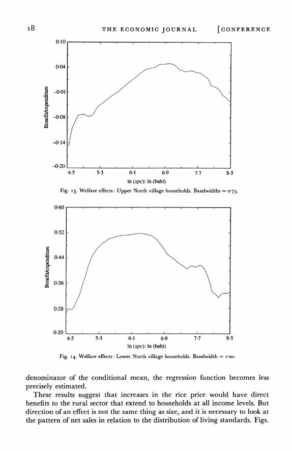
situation in the Lower North, where a good deal more rice is produced, and where more than half of the households are net sellers, a fraction that once again does not vary very much with living standards. Comparable graphs for the other regions are given in the Graphical Appendix: the Central region generates a regression that looks very like that for the Lower North, although both curves dip more sharply towards the upper end of the distribution. The


1*25-

D0-77-

0-51 8

Fig. I I. Net purchases

0.4 I r X _

1)-R

= 0.2 /\ 0-1

0-2

4*5 5 3 6-1 6.9 7.7 8-5 In (xpc): In (baht)

Fig. 12. Welfare effects: All village households. Bandwidth =-5.

South and the North East regions look very like the overall sectoral picture in Fig. 7. Rural households on the fringes of Bangkok also produce a great deal of rice. About 45 0 of such households are producers, and essentially all are net sellers. In interpreting these regressions, not too much attention should be paid to extreme variability in the regression function at either very high or very low levels of per capita expenditure. As we move to the tails of the distribution, the estimated density becomes smaller, and since this estimate enters into the


0.10

0.04

3 0-08 -

-0-14J

-0 20 4-5 5-3 641 6-9 7.7 8.5

In (xpc): In (baht)

Fig. 13. Welfare effects: Upper North village households. Bandwidths = o075.

0.60 I

0.52

0044 /\

0.36

0.28

0 20, , , , , 4.5 5.3 6.1 6.9 7-7 8.5

In (xpc): In (baht)

Fig. I4. Welfare effects: Lower North village households. Bandwidth I-Oo.

denominator of the conditional mean, the regression function becomes less precisely estimated.

These results suggest that increases in the rice price would have direct benefits to the rural sector that extend to households at all income levels. But direction of an effect is not the same thing as size, and it is necessary to look at the pattern of net sales in relation to the distribution of living standards. Figs.

1989] RICE DISTRIBUTION IN THAILAND I9

0-100

0.06

0.02

-0.02

-0606

-0.10 . 4-5 5-3 6.1 6.9 7.7 8.5

In (xpc): In (baht)

Fig. I5. Welfare effects: Upper North East village households. Bandwidth = 0-75.

O 15 -. r

0-12 -

0.09 \

8 0-06

0-03

0-00 4-5 5-3 6-1 6-9 7-7 8.5

In (xpc): In (baht)

Fig. I6. Welfare effects: Lower North East village households. Bandwidth = i-oo.

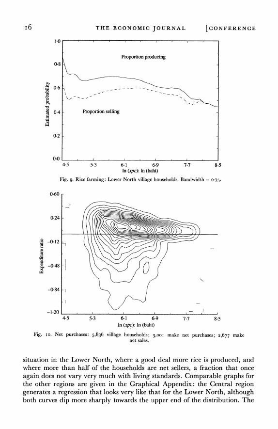
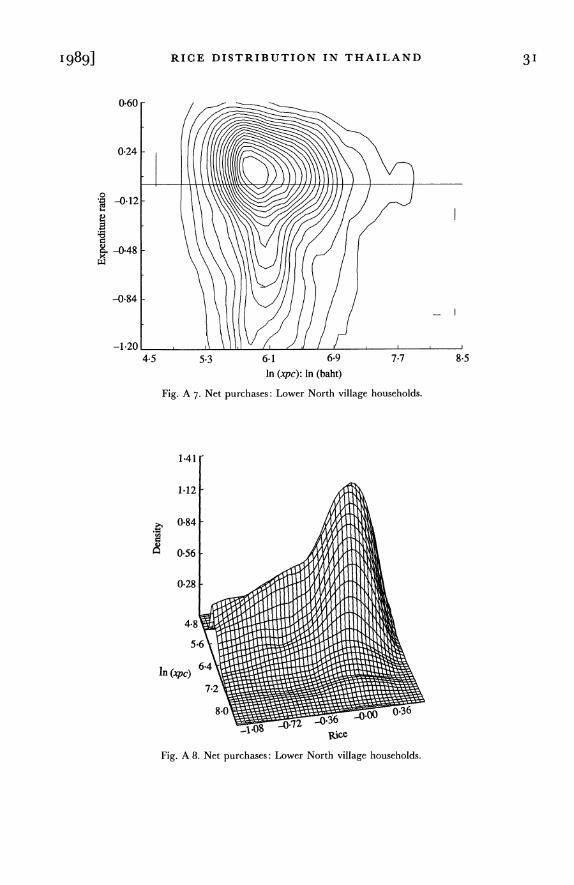
io and i i show, for the village sector, the joint density of the net expenditure ratio for rice and the logarithm of xpc. The contours in Fig. i o are as before, and the horizontal line is the zero net purchase line that divides net buyers (5I %) and net sellers (46 %) ; 3 % of households are on the line. Although it makes little difference, these households are not included when estimating the density. Fig. i i contains the same information as Fig. io, from a three dimensional perspective observed from above the right hand side of the zero


0.25 , .

0.20 -

0.15-

to 0.10

0-05

4-5 5.3 6.1 6.9 7-7 8.5

In (xpc): In (baht)

Fig. I 7. Welfare effects: Centre West village households. Bandwidth = I-oo.

0.40 ,

0.31 -

0.22 -

X 0.13 -

0.04

-0-05 , , , 4-5 5.3 6-1 6.9 7.7 8.5

In (xpc): In (baht)

Fig. i8. Welfare effects: Centre Middle village households. Bandwidth --OO.

line shown in Fig. io. I have not included the corresponding estimates for sanitary districts and municipal areas. For the latter, and apart from a scattering of outliers, the net purchase contours look like the consumption contours in Fig. 5; there is little rice production in urban areas. For sanitary districts, the shape of the density is much the same as in Fig. io, but the lower half of the graph is much foreshortened, and only a quarter of households are net sellers of rice.

I989] RICE DISTRIBUTION IN THAILAND 2I

0.60

0.46

0.1

0-04 -01)

4-5 5-3 6-1 6-9 7-7 8-5

In (xpc): In (baht)

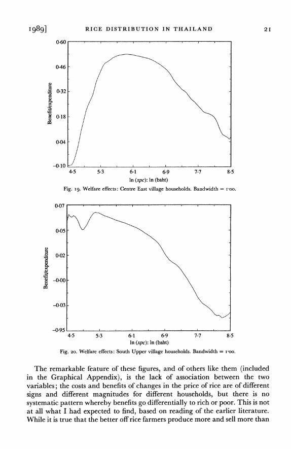
Fig. I9. Welfare effects: Centre East village households. Bandwidth = I-oo.

0'07

0305

-0.00

-0.03-

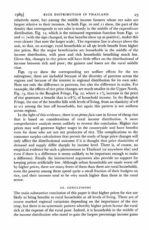
-095,.,.,.I, .I.,I

4-5 5-3 6.1 6-9 7-7 8-5 ln (xpc): In (baht)

Fig. 20. Welfare effects: South Upper village households. Bandwidth = I-oO.

The remarkable feature of these figures, and of others like them (included in the Graphical Appendix), is the lack of association between the two variables; the costs and benefits of changes in the price of rice are of different signs and different magnitudes for different households, but there is no systematic pattern whereby benefits go differentially to rich or poor. This is not at all what I had expected to find, based on reading of the earlier literature. While it is true that the better off rice farmers produce more and sell more than


0-002

*~-O040

-0.06

-O08

-0.10 / . . 4.5 5.3 6-1 6.9 7-7 8.5

In (xpc): In (baht)

Fig. 21. Welfare effects: South Lower village households. Bandwidth i-oo.

1-0

0-8

0-61\X

0.2

0-0 I I 4.5 5.3 6-1 6.9 7-7 8.5

In (xpc): In (baht)

Fig. 22. Welfare effects: Bangkok Fringe village households. Bandwidth = I-oo.

-do smaller, poorer farmers, and while it is also true that, among rice farmers, the richer (and presumably larger), farmers are more likely to be net sellers of rice, it is nevertheless not the case that increases in rice prices tip the distribution of real income towards the rich. Part of the reason is that there are relatively few rice farmers among the rich, so that the fractions of households who are net sellers of rice does not increase with income, but it is also true that the ratio of net sales to household income is largest, not among the rich who produce


relatively more, but among the middle income farmers whose net sales are largest relative to their incomes. As both Figs. io and i i show, the part of the density that corresponds to net sales is mostly in the middle of the expenditure distribution. Fig. I 2, which is the estimated regression function from Figs. io and i i (with the sign changed, so that benefits show up as positive), makes this even clearer (but note the larger scale). The regression line is always above the axis, so that, on average, rural households at all xpc levels benefit from higher rice prices. But the major beneficiaries are households in the middle of the income distribution, with poor and rich households benefiting much less. Given this, changes in rice prices will have little effect on the distributional of income between rich and poor; the gainers and losers are the rural middle class.

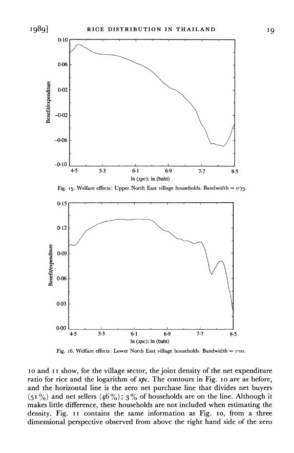
Figs. I 3-22 show the corresponding net welfare effects for the ten subregions; these are included because of the diversity of patterns across the regions and because of the interest in regional distribution for its own sake. Note not only the difference in patterns, but also the difference in scales. For example, the effects of rice price changes are much smaller in the Upper North, Fig. I 3, than in the Bangkok Fringe, Fig. 22, where a i % increase in the price of rice generates a benefit that is o-8 % of household income. In the Bangkok Fringe, the size of the benefits falls with levels of living, from an elasticity of o-8 to 0-2 among the best off households, but again this pattern is not uniform across regions.

In the light of this evidence, there is no primafacie case in favour of cheap rice that is based on considerations of rural income distribution. A more comprehensive analysis seems unlikely to reverse this conclusion. Higher rice prices may well generate higher wages in the countryside and have benefits even for those who are not net producers of rice. The complications to the consumer surplus calculations that permit the study of large price changes will only affect the distributional outcome if it is thought that price elasticities of demand and supply differ sharply by income level. There is, of course, no empirical evidence for such a phenomenon in Thailand (or anywhere else) and even if there is a difference it seems unlikely to be important enough to make a difference. Finally the intersectoral arguments also provide no support for keeping prices artificially low. Although urban households are made worse off by higher prices, there are many fewer of them than there are rural households, even the poorest among them spend quite a small fraction of their budgets on rice, and their incomes tend to be very much higher than those in the rural sector.

III. CONCLUSIONS

The main substantive conclusion of this paper is that higher prices for rice are likely to bring benefits to rural households at all levels of living. There are of course marked regional variations depending on the importance of the rice crop, but there is no systematic pattern whereby higher prices favour the rural rich at the expense of the rural poor. Indeed, it is households in the middle of the income distribution who stand to gain the largest percentage income gains


from increase in the price of rice. This result is summarised for the village sector as a whole in Fig. I2, and for the various regions of the Kingdom in Figs. I3

and 22. It is interesting to speculate on whether these results would have been

apparent using different and more familiar techniques. Consider, for example, the data displayed in Fig. I 2. In principle, such information could be gleaned from a cross-tabulation of the net consumption ratio on the logarithm of household per capita expenditure. In practice, cross-tabulations do not convey information as transparently as do the graphics. Furthermore, 'bin' sizes have to be selected for the cross-tabulation, and it is not difficult to construct examples where an inappropriate or unlucky choice can lead to the loss of important information. The smooth nature of Fig. I2 is a great advantage in this regard. If, as an alternative to cross-tabulation, we had used descriptive regressions, the results could have been much worse. The relationship depicted in Fig. I2 is far from linear, nor can it be well approximated by any low order polynomial. Without the graphical information, a likely outcome could be a regression making the net sales ratio a quadratic function of In (xpc). Such a form fits the main body of the data well, a fit that would be reflected in the usual statistics. But the behaviour of a fitted parabola in the tails of the distribution would be very different from the non-parametric regression shown in the Figure, and might well show losses for both rich and poor households. Since these are the two groups in which we are most interested, such a result would be most unfortunate.

The non-parametric techniques are probably at their best in these simple two-variable situations, and it is much more difficult to use them well, or to display the results, in problems that involve more variables and more dimensions. Nevertheless, there is a wide variety of policy issues that can be illuminated by flexible displays of bivariate relationships. There are also important theoretical questions that can be tackled using the same techniques. An elegant example is provided by a recent paper by Hildenbrand and Hildenbrand (I986) who test for an aggregate version of the law of demand using non-parametric estimates of densities and Engel curves from British survey data. There are many problems that non-parametric estimation cannot solve, but it seems clear that techniques are still far from overused among economists.

Princeton University

REFERENCES

Hardle, W. (i 987). Applied non-parametric regression, Manuscript, Fakultat Rechts- und Statts- wissenschaften, University of Bonn.

Hildenbrand, K. and Hildenbrand, W. (I986). 'On the mean income effect: a data analysis of the U.K. Family Expenditure Survey.' In Contributions to Mathematical Economics: in Honor of Gerard Debreu (ed. W. Hildenbrand and A. Mas-Colell), pp. 247-68. Amsterdam: North-Holland.

Silverman, B. W. (I986). Density Estimation for Statistics and Data Analysis. London and New York: Chapman and Hall.

Siamwalla, A. and Setboonsarng, S. (I987). Agricultural Pricing Policies in Thailand I96u-84. Bangkok: Thai Development Research Institute.

Trairatvorakul, P. (1984). The Effects of Income Distribution and Nutrition of Alternative Rice Price Policies in Thailand. Washington, D.C.: International Food Policy Research Institute.

19891 RICE DISTRIBUTION IN THAILAND 25

APPENDIX I

Non-parametric Estimation of Regressions and Densities The techniques described here are standard in the statistical literature, and excellent discussions can be found in Silverman (I986), for density estimation, and Hardle (I987), for regression. My aim here is to give only a brief explanation of what was done to generate the figures used in the main text and hence to make this paper reasonably self-contained.

One simple non-parametric regression technique that is familiar to everyone is the smoothing of a time-series by calculation of a moving average. For example, if data are available on daily stock returns, some of the noisiness of the series could be removed by plotting for each day not its own return, but the average of the returns for the k previous days, the day itself, and the k succeeding days. The bigger is k, the smoother will be the resulting plot. Exactly the same idea can be applied to the Engel curves estimated here, even though there is no natural ordering of observations, and in spite of their unequal spacing. Consider, for example, the construction of the rice share Engel curves illustrated in Fig. 2. At each point along the x (In xpc)-axis, there will be some nearby households, and an estimate of the Engel curve is computed by taking the (conditional) average of their rice budget shares. There are various ways of deciding which households to include, and how to calculate the average, but the same principles of smoothing that applied to the simple moving average also apply here. In particular, the more households included in the average, the smoother will be the regression.

In this paper, I have used 'kernel' estimators. These are conceptually straightforward, easily (although not necessarily inexpensively) computed, and can be applied to both density and regression function estimation. The idea is to set a 'bandwidth' parameter that determines how near observations have to be in order to contribute to the average at each point. In the context of Fig. 2, the simplest kernel estimator would be to set some bandwidth, say O-2o, and at each value of In (xpc) to calculate the average of the rice shares for households whose ln (xpc) is within 0X20 of the value. Such an estimator can be improved on by calculating a weighted average that gives greater weight to households the closer is their value of ln (xpc) to the value that is being considered. Formally, the estimate of the regression corresponding to a point X, m- (X), say, is

mn(X) = -wi (X, Xi) Yi, (A i)

where n is the sample size, Xi and Yi are the x and y values for observation i, and i runs over the whole sample. In the method described above, the (non- negative) weights wi will be zero for Xi far enough away from X, though it is also possible to allow all observations to contribute and simply let the weights decline with the distance between X and Xi.

The estimator (A i) is a very general one, and is described as a kernel estimator when the weights take the specific form

wi (X) Xi) = Kh (X-Xi)1/Kh(X-Xj)v (A 2)


where Kh is the kernel, and h is the bandwidth. Kh is a symmetric monotone decreasing function that integrates to unity over the range of its argument. In the calculations here I have used the Epanechnikov kernel which is defined by

X_Xt2 Kh(X-Xi) h I(IX-Xil ? h), (A 3)

where I is an indicator function such that I = i if X and Xi are within h of one another, and otherwise I = o. The 3/4 h is irrelevant for the purposes of calculating the weights in (A 2), but its presence is required to guarantee that the integral of Kh(X-Xi) be unity.

The formulae (A i)-(A 3) are used for all the non-parametric regressions discussed in the main text, and illustrated in Figs. 2, 7-9, I2-22, and Appendix Figs. A i-A 8. In Figs. 2 and I 2, the dependent variable y is either the rice share or the net consumption ratio of rice, while in Figs. 7-9, where I am estimating probabilities, the dependent variable is simply one or zero depending on whether the household does or does not grow and sell rice. The graphs are constructed by calculating (A i) for IOO equally spaced values of ln (xpc) and plotting the result. All calculations were programmed in GAUSS on a 386-series PC and were plotted using GAUSS graphics. The regression estimates are inexpensive to calculate, requiring about one minute of computation time. I selected bandwidths by trial and error, using screen plots to choose a value of h that appeared to give enough smoothness without obscuring detail. While there exist techniques for automatic bandwidth selection (see Silverman or Hardle), they tend to be computationally expensive, and early experiments with one such (cross-validation) showed that the informal methods were unlikely to be misleading, at least for the essentially graphical purposes of this paper.

Non-parametric estimates of density functions such as those in Fig. i follow very much the same principles. At each point on the x-axis, a count is made of how many households are nearby, and if this is expressed as a ratio of the sample size, an estimate of the density is obtained. Again, it is a good idea to give closer households greater weight, and a kernel function can be used to achieve this. Indeed, one of the great advantages of kernel regression estimation is that it automatically yields a density estimate as a by-product. This is the

estimatefh(X) given by, cf. (A 2),

fh(X) = n hK (Xi-X), (A 4)

where n is the sample size, and the fact that Kh (.) integrates to unity is now required in order to generate a proper estimate of the density. This formula is used to produce the univariate densities in Fig. i, and the results calculated at the same time as the regressions in Fig. 2.

The bivariate densities in Figs. 3-6 and in Figs. Io and i i are calculated according to the same general principles. A grid is constructed over the range of the two variables, and at each point on the grid, a (weighted) count is made of the observations within a neighbourhood of the point. The fineness of the


grid determines the definition of the contour and surface plots; here I used an 89 by 89 grid, which is the largest that can be handled by the GAUSS graphics routines. Since a complete pass through the sample has to be made for every point on the grid, these calculations are much more expensive than those for the non-parametric regressions, requiring some I 20 minutes of 386 machine time for the village sector which has 5,836 observations. A kernel weighting function is again used. The bivariate Epanechnikov kernel is given by, see Silverman (1 986, p. 76),

K(di) = (2/rh 2) (I -di' di) I(di' di < I), (A 5)

where di is a two element vector of deviations of Xi - X and Yi - Y each divided by the bandwidth h. Note that this kernel counts observations if they are within a circular region centred at the current point and with radius h. This is not likely to be very useful if the two variables are measured in very different units or if the distribution of the two variables is highly correlated, both of which are true in the current context. The natural way around the problem is to use the sample covariance matrix of the two variables as a metric, or equivalently to transform the units and axes so that the units are the same and the variables orthogonal. The density estimate at the point Z = (X, Y)' is then given by, see Silverman, equation (4.7),

f^(z) = (det S) -2k[h-2 (Z-Zi)'S-1 (Z-Zi)], (A 6)

where k(d'd) = K(d), where S is the sample variance covariance matrix of the two variables.

APPENDIX II

Additional Graphical Material'

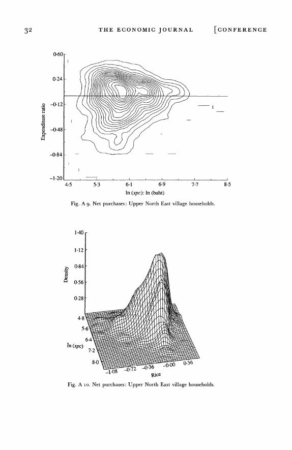
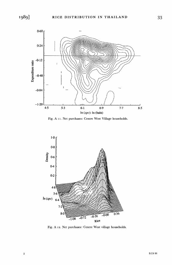
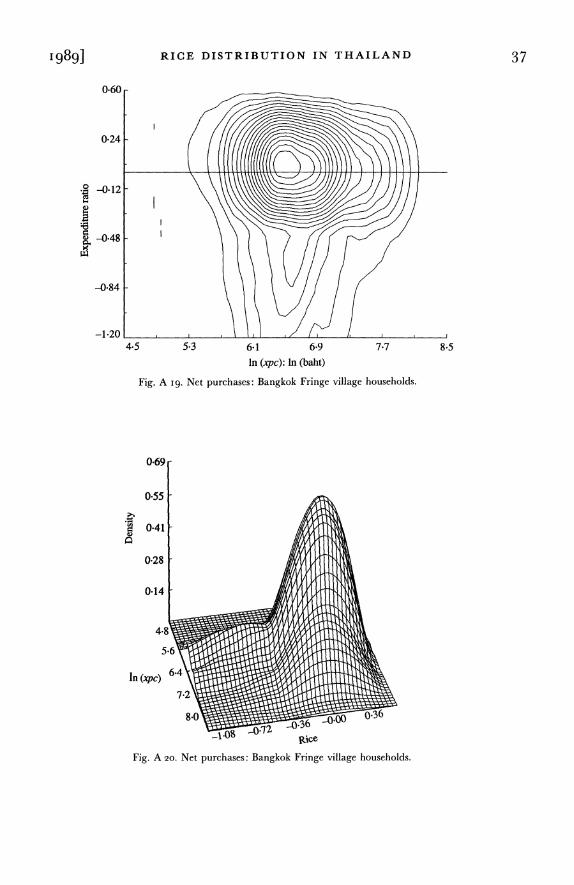
Figs. A i-A 6 correspond to Figs. 7-9 in the text. They show proportions of households producing and selling rice for the following regions: Upper North East, Lower North East, Central West, Central East, Central Middle, Upper South, Lower South and Bangkok Fringe. Figs. A 7-A 20 are the regional versions of Figs. Io and I I in the text. They show the joint distributions of the net rice consumption ratio and the logarithm of household per capita expenditure for the Upper and Lower North followed by the ten regions listed above.

1 A full set of graphical material is available from the author on request.



SM 0.6

0-\

i

06 S------------

0.4 Proportion selling

0.2 -

0.0 4-5 5.3 6.1 6-9 7.7 8-5

In (xpc): In (baht)

Fig. A i. Rice farming: Upper North East village households. Bandwidth = i-oo.

Proportion producing 0.8

0.6

t 0.4 Proportion selling

0.2

0-0 l l l 4.5 5-3 6-1 6-9 7-7 8.5

In (xpc): In (baht)

Fig. A 2. Rice farming: Central West village households. Bandwidth = I-oo.


1.G

0*8

i 0.6 - oportion producing

-D

,a 04 Proportion selling

0-2

0 0 4.5 5.3 6-1 6-9 7.7 8.5

In (xpc): In (baht)

Fig. A 3. Rice farming: Central Middle village households. Bandwidth = o75.

0.8 Proportion producing

0

a 0-4 Proportion selling - -_

0-2-

0.0 4-5 5-3 6-i 6-9 7-7 8-5

In (xpc): In (baht)

Fig. A 4. Rice farming: South Upper village households. Bandwidth = 0-75.


1.0

0.8

E 0.6 Proportion producing

0-4 - Proportion selling

0.2

4-5 5.3 6.1 6-9 7.7 8.5 In (xpc): In (baht)

Fig. A 5. Rice farming: South Lower village households. Bandwidth = -oo.

1.0

0.8

i 0-6 - Proportion producing

X 0-4 Prprto selling '

0X - 0.0

02

4.5 5.3 6.1 6.9 7.7 8.5 In (xpc): ln (baht)

Fig. A 6. Rice farming: Bangkok Fringe village households. Bandwidth = o075.

I989] RICE DISTRIBUTION IN THAILAND

0.60 -

0-24

i -0.12"

-0-48

-0.84

-1.20 4.5 5.3 6-1 6.9 7.7 8-5

In (xpc): In (baht)

Fig. A 7. Net purchases: Lower North village households.

1-41-

1-12 -

7.28

Rice

Fig. A 8. Net purchases: Lower North village households.


0.60

024 -

0 |-1 -

-0-48-

{)-84 -

-1-20 . , 4-5 5-3 6-1 6.9 7-7 8.5

In (xpc): In (baht)

Fig. A 9. Net purchases: Upper North East village households.

1-40

1-12-

,0-84-

0.

li (xpc) 7.2

Fig. A io. Net purchases: Upper North East village households.


0-60

0.24

-0.12

-0.48-

-0*84-

-1-20 ,|,\, 4.5 5*3 6-1 6-9 7*7 8.5

In (xpc): In (baht)

Fig. A i i. Net purchases: Centre West Village households.

1.0

08

0-4-

0.2

In (xpc) 6.4

7.2

8.0 36b

6

1 ice

Fig. A 12. Net purchases: Centre West village households.

2 ECS 99


0-60

0.24 -

A -48

-0*84 -

-1-201 4-5 5-3 6-1 6-9 7-7 8.5

In (xpc): In (baht)

Fig. A 13. Net purchases: Centre Middle village households.

1.0

0.8

0-6-

0.4

0.2

In (xpc) 7.2

8.0 Fig. A 14. Net purchases: Centre Middle village households.


0*60

0*24-

-0 48;

-0-84

-1-20 4.5 5-3 6.1 6.9 7-7 8.5

In (xpc): In (baht)

Fig. A I5. Net purchases: Upper South village households.

1-92

1.53 -

1-15-

0.77

0.38

7.2

8.0 1 Fig. A I6. Net purchases: Upper South village households.

2-2


0.60

0*24

0 _ _ _ _

-0-12 - __

-0.48

-084

-1-20 4.5 5-3 6.1 6-9 7-7 8.5

In (xpc): In (baht)

Fig. A 1 7. Net purchases: Lower South village households.

1-92-

1-53

1-15

077 .

In (xpc

rice

Fig. A i8. Net purchases: Lower South village households.


0.60

0H24

*0 -0.12-

-0.48

-0.84

-1-20 4.5 53 6-1 6-9 7-7 8.5

In (xpc): In (baht)

Fig. A I9. Net purchases: Bangkok Fringe village households.

0-69

0-55

0-41

0.28 -

0-14-

In (xpc)64 7*2

R:Ice

Fig. A 20. Net purchases: Bangkok Fringe village households.

RICE PRICES AND INCOME DISTRIBUTION IN …deaton/downloads/Rice_Prices...The Economic Journal, 99 (Conference I 989), 1-37 Printed in Great Britain RICE PRICES AND INCOME DISTRIBUTION

Documents