UNCLASSIFIED Software Cost Estimation Metrics Manual UNCLASSIFIED Distribution Statement A: Approved for public release Software Cost Estimation Metrics Manual Analysis based on data from the DoD Software Resource Data Report This manual describes a method that takes software cost metrics data and creates cost estimating relationship models. Definitions of the data used in the methodology are discussed. The cost data definitions of other popular Software Cost Estimation Models are also discussed. The data collected from DoD’s Software Resource Data Report are explained. The steps for preparing the data for analysis are described. The results of the data analysis are presented for different Operating Environments and Productivity Types. The manual wraps up with a look at modern estimating challenges.

Welcome message from author
This document is posted to help you gain knowledge. Please leave a comment to let me know what you think about it! Share it to your friends and learn new things together.
Transcript

UNCLASSIFIED
Software Cost Estimation Metrics Manual
UNCLASSIFIED
Distribution Statement A: Approved for public release
Software Cost Estimation Metrics
Manual Analysis based on data from the DoD Software
Resource Data Report
This manual describes a method that takes software cost metrics data and
creates cost estimating relationship models. Definitions of the data used in the
methodology are discussed. The cost data definitions of other popular Software
Cost Estimation Models are also discussed. The data collected from DoD’s Software Resource Data Report are explained. The steps for preparing the data
for analysis are described. The results of the data analysis are presented for
different Operating Environments and Productivity Types. The manual wraps
up with a look at modern estimating challenges.
UNCLASSIFIED
Software Cost Estimation Metrics Manual
UNCLASSIFIED
Distribution Statement A: Approved for public release
Contents 1 Introduction ........................................................................................................................................ 1
2 Metrics Definitions ............................................................................................................................. 2
2.1 Size Measures ............................................................................................................................. 2
2.2 Source Lines of Code (SLOC) ................................................................................................... 2
2.2.1 SLOC Type Definitions ......................................................................................................... 2
2.2.2 SLOC Counting Rules ........................................................................................................... 3
2.2.2.1 Logical Lines ................................................................................................................... 3
2.2.2.2 Physical Lines ................................................................................................................. 4
2.2.2.3 Total Lines ....................................................................................................................... 4
2.2.2.4 Non‐Commented Source Statements (NCSS) ............................................................ 4
2.3 Equivalent Size ........................................................................................................................... 5
2.3.1 Definition and Purpose in Estimating ................................................................................ 5
2.3.2 Adapted SLOC Adjustment Factors ................................................................................... 6
2.3.3 Total Equivalent Size ............................................................................................................ 7
2.3.4 Volatility ................................................................................................................................. 7
2.4 Development Effort ................................................................................................................... 7
2.4.1 Activities and Lifecycle Phases ............................................................................................ 7
2.4.2 Labor Categories .................................................................................................................... 8
2.4.3 Labor Hours ........................................................................................................................... 9
2.5 Schedule ...................................................................................................................................... 9
3 Cost Estimation Models .................................................................................................................. 10
3.1 Effort Formula .......................................................................................................................... 10
3.2 Cost Models .............................................................................................................................. 10
3.2.1 COCOMO II ......................................................................................................................... 11
3.2.2 SEER‐SEM ............................................................................................................................ 12
3.2.3 SLIM ...................................................................................................................................... 12
3.2.4 True S .................................................................................................................................... 13
3.3 Model Comparisons ................................................................................................................. 13
3.3.1 Size Inputs ............................................................................................................................ 13
3.3.1.1 COCOMO II .................................................................................................................. 14
3.3.1.2 SEER‐SEM ..................................................................................................................... 14
3.3.1.3 True S ............................................................................................................................. 16
3.3.1.4 SLIM ............................................................................................................................... 19
3.3.2 Lifecycles, Activities and Cost Categories ....................................................................... 19
4 Software Resource Data Report (SRDR) ....................................................................................... 23
UNCLASSIFIED
Software Cost Estimation Metrics Manual
UNCLASSIFIED
Distribution Statement A: Approved for public release
4.1 DCARC Repository .................................................................................................................. 23
4.2 SRDR Reporting Frequency .................................................................................................... 24
4.3 SRDR Content ........................................................................................................................... 25
4.3.1 Administrative Information (SRDR Section 3.1) ............................................................. 25
4.3.2 Product and Development Description (SRDR Section 3.2) .......................................... 26
4.3.3 Product Size Reporting (SRDR Section 3.3) ..................................................................... 27
4.3.4 Resource and Schedule Reporting (SRDR Section 3.4) .................................................. 28
4.3.5 Product Quality Reporting (SRDR Section 3.5 ‐ Optional) ............................................ 28
4.3.6 Data Dictionary .................................................................................................................... 29
5 Data Assessment and Processing................................................................................................... 30
5.1 Workflow ................................................................................................................................... 30
5.1.1 Gather Collected Data ......................................................................................................... 30
5.1.2 Inspect each Data Point ...................................................................................................... 31
5.1.3 Determine Data Quality Levels ......................................................................................... 33
5.1.4 Correct Missing or Questionable Data ............................................................................. 34
5.1.5 Normalize Size and Effort Data ......................................................................................... 34
5.1.5.1 Converting to Logical SLOC ....................................................................................... 34
5.1.5.2 Convert Raw SLOC into Equivalent SLOC .............................................................. 37
5.1.5.3 Adjust for Missing Effort Data ................................................................................... 39
5.2 Data Segmentation ................................................................................................................... 39
5.2.1 Operating Environments (OpEnv) .................................................................................... 40
5.2.2 Productivity Types (PT) ..................................................................................................... 41
5.2.2.1 Finding the Productivity Type ................................................................................... 44
6 Cost Estimating Relationship Analysis ......................................................................................... 46
6.1 Application Domain Decomposition..................................................................................... 46
6.2 SRDR Metric Definitions ......................................................................................................... 46
6.2.1 Software Size ........................................................................................................................ 46
6.2.2 Software Development Activities and Durations ........................................................... 46
6.3 Cost Estimating Relationships (CER) .................................................................................... 48
6.3.1 Model Selection ................................................................................................................... 48
6.3.2 Model‐Based CERs Coverage ............................................................................................ 49
6.3.3 Software CERs by OpEnv .................................................................................................. 50
6.3.3.1 Ground Site (GS) Operating Environment ............................................................... 50
6.3.3.2 Ground Vehicle (GV) Operating Environment ........................................................ 51
6.3.3.3 Aerial Vehicle (AV) Operating Environment ........................................................... 52
6.3.3.4 Space Vehicle Unmanned (SVU) Operating Environment .................................... 53
6.3.4 Software CERs by PT Across All Environments ............................................................. 53

UNCLASSIFIED
Software Cost Estimation Metrics Manual
UNCLASSIFIED
Distribution Statement A: Approved for public release
6.4 Productivity Benchmarks ........................................................................................................ 56
6.4.1 Model Selection and Coverage .......................................................................................... 56
6.4.2 Data Transformation ........................................................................................................... 57
6.4.3 Productivity Benchmark Statistics .................................................................................... 58
6.4.4 Software Productivity Benchmark Results by Operating Environment ..................... 58
6.4.5 Software Productivity Benchmarks Results by Productivity Type .............................. 59
6.4.6 Software Productivity Benchmarks by OpEnv and PT .................................................. 61
6.5 Future Work .............................................................................................................................. 61
7 Modern Estimation Challenges ...................................................................................................... 62
7.1 Changing Objectives, Constraints and Priorities ................................................................. 62
7.1.1 Rapid Change, Emergent Requirements, and Evolutionary Development ................ 62
7.1.2 Net‐centric Systems of Systems (NCSoS) ......................................................................... 65
7.1.3 Model‐Driven and Non‐Developmental Item (NDI)‐Intensive Development ........... 65
7.1.4 Ultrahigh Software Systems Assurance ........................................................................... 66
7.1.5 Legacy Maintenance and Brownfield Development ...................................................... 67
7.1.6 Agile and Kanban Development ....................................................................................... 68
7.1.7 Putting It All Together at the Large‐Project or Enterprise Level .................................. 68
7.2 Estimation Approaches for Different Processes .................................................................. 69
8 Conclusions and Next Steps ........................................................................................................... 73
9 Appendices ....................................................................................................................................... 74
9.1 Acronyms .................................................................................................................................. 74
9.2 Automated Code Counting .................................................................................................... 79
9.3 Additional Adapted SLOC Adjustment Factors .................................................................. 79
9.3.1 Examples ............................................................................................................................... 81
9.3.1.1 Example: New Software .............................................................................................. 81
9.3.1.2 Example: Modified Software ...................................................................................... 81
9.3.1.3 Example: Upgrade to Legacy System ........................................................................ 81
9.4 SRDR Data Report .................................................................................................................... 82
9.4.1 Proposed Modifications ...................................................................................................... 86
9.5 MIL‐STD‐881C WBS Mapping to Productivity Types ........................................................ 88
9.5.1 Aerial Vehicle Manned (AVM) .......................................................................................... 88
9.5.2 Ordinance Vehicle Unmanned (OVU) ............................................................................. 90
9.5.3 Ordinance Vehicle Unmanned (OVU) ............................................................................. 92
9.5.4 Maritime Vessel Manned (MVM) ..................................................................................... 93
9.5.5 Space Vehicle Manned / Unmanned (SVM/U) and Ground Site Fixed (GSF) ............ 94
9.5.6 Ground Vehicle Manned and Unmanned (GVM/U) ...................................................... 95
9.5.7 Aerial Vehicle Unmanned(AVU) & Ground Site Fixed (GSF) ...................................... 97
UNCLASSIFIED
Software Cost Estimation Metrics Manual
UNCLASSIFIED
Distribution Statement A: Approved for public release
9.5.8 Maritime Vessel Unmanned (MVU) and Maritime Vessel Manned (MVM) .............. 98
9.5.9 Ordinance Vehicle Unmanned (OVU) ............................................................................. 99
9.5.10 Ground Site Fixed (GSF) ................................................................................................... 100
9.5.11 Applies to ALL Environments......................................................................................... 100
9.6 Productivity (Pr) Benchmark Details .................................................................................. 101
9.6.1 Normality Tests on Productivity Data ........................................................................... 101
9.6.1.1 Operating Environments (all Productivity Types) ................................................ 101
9.6.1.2 Productivity Types (all Operating Environments) ................................................ 102
9.6.1.3 Operating Environment – Productivity Type Sets ................................................ 102
9.6.2 Statistical Summaries on Productivity Data .................................................................. 102
9.6.2.1 Operating Environments ........................................................................................... 103
9.6.2.2 Productivity Types ..................................................................................................... 108
9.6.2.3 Operating Environment ‐ Productivity Type Sets ................................................. 114
9.7 References................................................................................................................................ 129
Acknowledgements The research and production of this manual was supported by the Systems Engineering
Research Center (SERC) under Contract H98230‐08‐D‐0171 and the US Army Contracting
Command, Joint Munitions & Lethality Center, Joint Armaments Center, Picatinny Arsenal, NJ,
under RFQ 663074.
Many people worked to make this manual possible. The contributing authors were:
Cheryl Jones, US Army Armament Research Development and Engineering Center
(ARDEC)
John McGarry, ARDEC
Joseph Dean, Air Force Cost Analysis Agency (AFCAA)
Wilson Rosa, AFCAA
Ray Madachy, Naval Post Graduate School
Barry Boehm, University of Southern California (USC)
Brad Clark, USC
Thomas Tan, USC
UNCLASSIFIED
Software Cost Estimation Metrics Manual
Introduction 1 UNCLASSIFIED
Distribution Statement A: Approved for Public Release
Software Cost Estimation Metrics Manual Analysis based on data from the DoD Software Resource Data Report
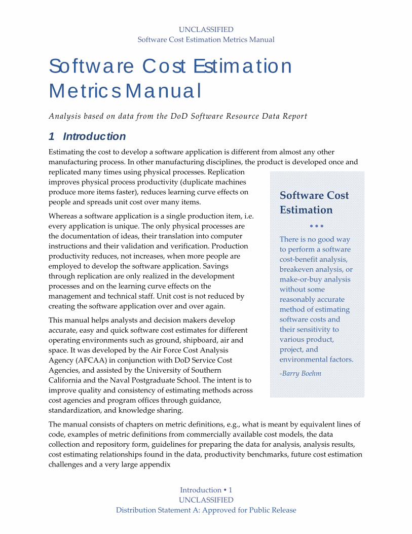
1 Introduction Estimating the cost to develop a software application is different from almost any other
manufacturing process. In other manufacturing disciplines, the product is developed once and
replicated many times using physical processes. Replication
improves physical process productivity (duplicate machines
produce more items faster), reduces learning curve effects on
people and spreads unit cost over many items.
Whereas a software application is a single production item, i.e.
every application is unique. The only physical processes are
the documentation of ideas, their translation into computer
instructions and their validation and verification. Production
productivity reduces, not increases, when more people are
employed to develop the software application. Savings
through replication are only realized in the development
processes and on the learning curve effects on the
management and technical staff. Unit cost is not reduced by
creating the software application over and over again.
This manual helps analysts and decision makers develop
accurate, easy and quick software cost estimates for different
operating environments such as ground, shipboard, air and
space. It was developed by the Air Force Cost Analysis
Agency (AFCAA) in conjunction with DoD Service Cost
Agencies, and assisted by the University of Southern
California and the Naval Postgraduate School. The intent is to
improve quality and consistency of estimating methods across
cost agencies and program offices through guidance,
standardization, and knowledge sharing.
The manual consists of chapters on metric definitions, e.g., what is meant by equivalent lines of
code, examples of metric definitions from commercially available cost models, the data
collection and repository form, guidelines for preparing the data for analysis, analysis results,
cost estimating relationships found in the data, productivity benchmarks, future cost estimation
challenges and a very large appendix
Software Cost
Estimation
There is no good way
to perform a software
cost‐benefit analysis,
breakeven analysis, or
make‐or‐buy analysis
without some
reasonably accurate
method of estimating
software costs and
their sensitivity to
various product,
project, and
environmental factors.
‐Barry Boehm

UNCLASSIFIED
Software Cost Estimation Metrics Manual
Metrics Definitions 2 UNCLASSIFIED
Distribution Statement A: Approved for Public Release
2 Metrics Definitions
2.1 Size Measures This chapter defines software product size measures used in Cost Estimating Relationship
(CER) analysis. The definitions in this chapter should be compared to the commercial cost
model definitions in the next chapter. This will help understand why estimates may vary
between these analysis results in this manual and other model results.
For estimation and productivity analysis, it is necessary to have consistent measurement
definitions. Consistent definitions must be used across models to permit meaningful
distinctions and useful insights for project management.
2.2 Source Lines of Code (SLOC) An accurate size estimate is the most important input to parametric cost models. However,
determining size can be challenging. Projects may be composed of new code, code adapted
from other sources with or without modifications, and automatically generated or translated
code.
The common measure of software size used in this manual is Source Lines of Code (SLOC).
SLOC are logical source statements consisting of data declarations and executables. Different
types of SLOC counts will be discussed later.
2.2.1 SLOC Type Definitions The core software size type definitions used throughout this manual are summarized in Table 1
below. These definitions apply to size estimation, data collection, and analysis. Some of the size
terms have different interpretations in the different cost models as described in Chapter 3.
Table 1 Software Size Types
Size Type Description
New Original software created for the first time. Adapted Pre-existing software that is used as-is (Reused) or changed (Modified).
Reused
Pre-existing software that is not changed with the adaption parameter settings: Design Modification % (DM) = 0% Code Modification % (CM) = 0%
Modified
Pre-existing software that is modified for use by making design, code and / or test changes: Design Modification % (DM) >= 0% Code Modification % (CM) > 0%
Equivalent A relative measure of the work done to produce software compared to the code-counted size of the delivered software. It adjusts the size of adapted software relative to developing it all new.

UNCLASSIFIED
Software Cost Estimation Metrics Manual
Metrics Definitions 3 UNCLASSIFIED
Distribution Statement A: Approved for Public Release
Table 1 Software Size Types
Size Type Description
Generated Software created with automated source code generators. The code to include for equivalent size consists of automated tool generated statements.
Converted Software that is converted between languages using automated translators.
Commercial Off-The-Shelf Software (COTS)
Pre-built commercially available software components. The source code is not available to application developers. It is not included for equivalent size. Other unmodified software not included in equivalent size are Government Furnished Software (GFS), libraries, operating systems and utilities.
The size types are applied at the source code file level for the appropriate system‐of‐interest. If a
component, or module, has just a few lines of code changed then the entire component is
classified as Modified even though most of the lines remain unchanged. The total product size
for the component will include all lines.
Open source software is handled, as with other categories of software, depending on the context
of its usage. If it is not touched at all by the development team it can be treated as a form of
COTS or reused code. However, when open source is modified it must be quantified with the
adaptation parameters for modified code and be added to the equivalent size. The costs of
integrating open source with other software components should be added into overall project
costs.
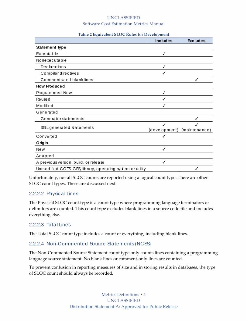
2.2.2 SLOC Counting Rules
2.2.2.1 Logical Lines
The common measure of software size used in this manual and the cost models is Source Lines
of Code (SLOC). SLOC are logical source statements consisting of data declarations and
executables. Table 2 shows the SLOC definition inclusion rules for what to count. Based on the
Software Engineering Institute (SEI) checklist method [Park 1992, Goethert et al. 1992], each
checkmark in the “Includes” column identifies a particular statement type or attribute included
in the definition, and vice‐versa for the “Excludes”.
UNCLASSIFIED
Software Cost Estimation Metrics Manual
Metrics Definitions 4 UNCLASSIFIED
Distribution Statement A: Approved for Public Release
Table 2 Equivalent SLOC Rules for Development
Includes Excludes
Statement Type Executable ✓
Nonexecutable Declarations ✓
Compiler directives ✓
Comments and blank lines ✓
How Produced Programmed New ✓
Reused ✓
Modified ✓
Generated Generator statements ✓
3GL generated statements ✓ (development)
✓ (maintenance)
Converted ✓
Origin New ✓
Adapted A previous version, build, or release ✓
Unmodified COTS, GFS, library, operating system or utility ✓
Unfortunately, not all SLOC counts are reported using a logical count type. There are other
SLOC count types. These are discussed next.
2.2.2.2 Physical Lines
The Physical SLOC count type is a count type where programming language terminators or
delimiters are counted. This count type excludes blank lines in a source code file and includes
everything else.
2.2.2.3 Total Lines
The Total SLOC count type includes a count of everything, including blank lines.
2.2.2.4 Non-Commented Source Statements (NCSS)
The Non‐Commented Source Statement count type only counts lines containing a programming
language source statement. No blank lines or comment‐only lines are counted.
To prevent confusion in reporting measures of size and in storing results in databases, the type
of SLOC count should always be recorded.
UNCLASSIFIED
Software Cost Estimation Metrics Manual
Metrics Definitions 5 UNCLASSIFIED
Distribution Statement A: Approved for Public Release
2.3 Equivalent Size A key element in using software size for effort estimation is the concept of equivalent size.
Equivalent size is a quantification of the effort required to use previously existing code along
with new code. The challenge is normalizing the effort required to work on previously existing
code to the effort required to create new code. For cost estimating relationships, the size of
previously existing code does not require the same effort as the effort to develop new code.
The guidelines in this section will help the estimator in determining the total equivalent size. All
of the models discussed in Chapter 3 have tools for doing this. However, for non‐traditional
size categories (e.g., a model may not provide inputs for auto‐generated code), this manual will
help the estimator calculate equivalent size outside of the tool and incorporate the size as part of
the total equivalent size.
2.3.1 Definition and Purpose in Estimating The size of reused and modified code is adjusted to be its equivalent in new code for use in
estimation models. The adjusted code size is called Equivalent Source Lines of Code (ESLOC).
The adjustment is based on the additional effort it takes to modify the code for inclusion in the
product taking into account the amount of design, code and testing that was changed and is
described in the next section.
In addition to newly developed software, adapted software that is modified and reused from
another source and used in the product under development also contributes to the productʹs
equivalent size. A method is used to make new and adapted code equivalent so they can be
rolled up into an aggregate size estimate.
There are also different ways to produce software that complicate deriving ESLOC including
generated and converted software. All of the categories are aggregated for equivalent size. A
primary source for the equivalent sizing principles in this section is Chapter 9 of [Stutzke 2005].
For usual Third Generation Language (3GL) software such as C or Java, count the logical 3GL
statements. For Model‐Driven Development (MDD), Very High Level Languages (VHLL), or
macro‐based development, count the generated statements A summary of what to include or
exclude in ESLOC for estimation purposes is in the table below.

UNCLASSIFIED
Software Cost Estimation Metrics Manual
Metrics Definitions 6 UNCLASSIFIED
Distribution Statement A: Approved for Public Release
Table 3 Equivalent SLOC Rules for Development
Source Includes Excludes New ✓
Reused ✓
Modified ✓
Generated Generator statements ✓
3GL generated statements ✓
Converted COTS ✓
Volatility ✓
2.3.2 Adapted SLOC Adjustment Factors The AAF factor is applied to the size of the adapted software to get its equivalent size. The cost
models have different weighting percentages as identified in the Chapter 3.
The normal Adaptation Adjustment Factor (AAF) is computed as:
Eq 1 AAF = (0.4 x DM) + (0.3 x CM) + (0.3 x IM)
Where
% Design Modified (DM) The percentage of the adapted software’s design which is modified in order to adapt it to the
new objectives and environment. This can be a measure of design elements changed such as
UML descriptions.
% Code Modified (CM) The percentage of the adapted software’s code which is modified in order to adapt it to the new
objectives and environment.
Code counting tools can be used to measure CM. See the chapter on the Unified Code Count
tool in Appendix 9.2 for its capabilities, sample output and access to it.
% Integration Required (IM) The percentage of effort required to integrate the adapted software into an overall product and
to test the resulting product as compared to the normal amount of integration and test effort for
software of comparable size.
Reused software has DM = CM = 0. IM is not applied to the total size of the reused software, but
to the size of the other software directly interacting with it. It is frequently estimated using a
percentage. Modified software has CM > 0.
UNCLASSIFIED
Software Cost Estimation Metrics Manual
Metrics Definitions 7 UNCLASSIFIED
Distribution Statement A: Approved for Public Release
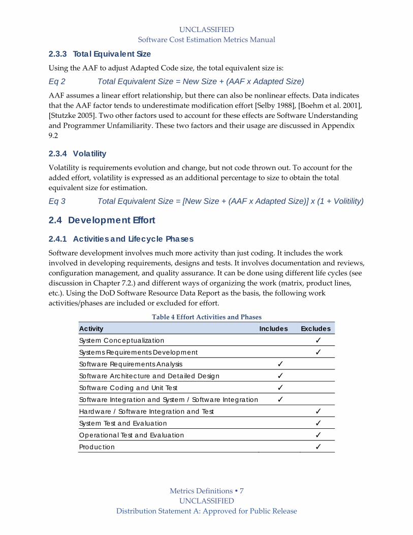
2.3.3 Total Equivalent Size Using the AAF to adjust Adapted Code size, the total equivalent size is:
Eq 2 Total Equivalent Size = New Size + (AAF x Adapted Size)
AAF assumes a linear effort relationship, but there can also be nonlinear effects. Data indicates
that the AAF factor tends to underestimate modification effort [Selby 1988], [Boehm et al. 2001],
[Stutzke 2005]. Two other factors used to account for these effects are Software Understanding
and Programmer Unfamiliarity. These two factors and their usage are discussed in Appendix
9.2
2.3.4 Volatility Volatility is requirements evolution and change, but not code thrown out. To account for the
added effort, volatility is expressed as an additional percentage to size to obtain the total
equivalent size for estimation.
Eq 3 Total Equivalent Size = [New Size + (AAF x Adapted Size)] x (1 + Volitility)
2.4 Development Effort
2.4.1 Activities and Lifecycle Phases Software development involves much more activity than just coding. It includes the work
involved in developing requirements, designs and tests. It involves documentation and reviews,
configuration management, and quality assurance. It can be done using different life cycles (see
discussion in Chapter 7.2.) and different ways of organizing the work (matrix, product lines,
etc.). Using the DoD Software Resource Data Report as the basis, the following work
activities/phases are included or excluded for effort.
Table 4 Effort Activities and Phases
Activity Includes Excludes System Conceptualization ✓
Systems Requirements Development ✓
Software Requirements Analysis ✓
Software Architecture and Detailed Design ✓
Software Coding and Unit Test ✓
Software Integration and System / Software Integration ✓
Hardware / Software Integration and Test ✓
System Test and Evaluation ✓
Operational Test and Evaluation ✓
Production ✓

UNCLASSIFIED
Software Cost Estimation Metrics Manual
Metrics Definitions 8 UNCLASSIFIED
Distribution Statement A: Approved for Public Release
Phase Includes Excludes Inception ✓
Elaboration ✓
Construction ✓
Transition ✓
Software requirements analysis includes any prototyping activities. The excluded activities are
normally supported by software personnel but are considered outside the scope of their
responsibility for effort measurement. Systems Requirements Development includes equations
engineering (for derived requirements) and allocation to hardware and software.
All these activities include the effort involved in documenting, reviewing and managing the
work‐in‐process. These include any prototyping and the conduct of demonstrations during the
development.
Transition to operations and operations and support activities are not addressed by these
analyses for the following reasons:
They are normally accomplished by different organizations or teams.
They are separately funded using different categories of money within the DoD.
The cost data collected by projects therefore does not include them within their scope.
From a life cycle point‐of‐view, the activities comprising the software life cycle are represented
for new, adapted, reused, generated and COTS (Commercial Off‐The‐Shelf) developments.
Reconciling the effort associated with the activities in the Work Breakdown Structure (WBS)
across life cycle is necessary for valid comparisons to be made between results from cost
models.
2.4.2 Labor Categories The labor categories included or excluded from effort measurement is another source of
variation. The categories consist of various functional job positions on a project. Most software
projects have staff fulfilling the functions of:
Project Managers
Application Analysts
Implementation Designers
Programmers
Testers
Quality Assurance personnel
Configuration Management personnel
Librarians
Database Administrators
Documentation Specialists
Training personnel
Other support staff
UNCLASSIFIED
Software Cost Estimation Metrics Manual
Metrics Definitions 9 UNCLASSIFIED
Distribution Statement A: Approved for Public Release
Adding to the complexity of measuring what is included in effort data is that staff could be
fulltime or part time and charge their hours as direct or indirect labor. The issue of capturing
overtime is also a confounding factor in data capture.
2.4.3 Labor Hours Labor hours (or Staff Hours) is the best form of measuring software development effort. This
measure can be transformed into Labor Weeks, Labor Months and Labor Years. For modeling
purposes, when weeks, months or years is required, choose a standard and use it consistently,
e.g. 152 labor hours in a labor month.
If data is reported in units other than hours, additional information is required to ensure the
data is normalized. Each reporting Organization may use different amounts of hours in
defining a labor week, month or year. For whatever unit being reported, be sure to also record
the Organization’s definition for hours in a week, month or year. See [Goethert et a 1992] for a
more detailed discussion.
2.5 Schedule Schedule data are the start and end date for different development phases, such as those discuss
in 2.4.1. Another important aspect of schedule data is entry or start and exit or completion
criteria each phase. The criteria could vary between projects depending on its definition. As an
example of exit or completion criteria, are the dates reported when:
Internal reviews are complete
Formal review with the customer is complete
Sign‐off by the customer
All high‐priority actions items are closed
All action items are closed
Products of the activity / phase are placed under configuration management
Inspection of the products are signed‐off by QA
Management sign‐off
An in‐depth discussion is provided in [Goethert et al 1992].

UNCLASSIFIED
Software Cost Estimation Metrics Manual
Cost Estimation Models 10 UNCLASSIFIED
Distribution Statement A: Approved for Public Release
3 Cost Estimation Models In Chapter 2 metric definitions were discussed for sizing software, effort and schedule. Cost
estimation models widely used on DoD projects are overviewed in this section. It describes the
parametric software cost estimation model formulas (the one that have been published), size
inputs, lifecycle phases, labor categories, and how they relate to the standard metrics
definitions. The models include COCOMO, SEER‐SEM, SLIM, and True S. The similarities and
differences for the cost model inputs (size, cost factors) and outputs (phases, activities) are
identified for comparison.
3.1 Effort Formula Parametric cost models used in avionics, space, ground, and shipboard platforms by the
services are generally based on the common effort formula shown below. Size of the software is
provided in a number of available units, cost factors describe the overall environment and
calibrations may take the form of coefficients adjusted for actual data or other types of factors
that account for domain‐specific attributes [Lum et al. 2001] [Madachy‐Boehm 2008]. The total
effort is calculated and then decomposed by phases or activities according to different schemes
in the models.
Eq 4 Effort = A x SizeB x C
Where
Effort is in person‐months
A is a calibrated constant
B is a size scale factor
C is an additional set of factors that influence effort.
The popular parametric cost models in widespread use today allow size to be expressed as lines
of code, function points, object‐oriented metrics and other measures. Each model has its own
respective cost factors and multipliers for EAF, and each model specifies the B scale factor in
slightly different ways (either directly or through other factors). Some models use project type
or application domain to improve estimating accuracy. Others use alternative mathematical
formulas to compute their estimates. A comparative analysis of the cost models is provided
next, including their sizing, WBS phases and activities.
3.2 Cost Models The models covered include COCOMO II, SEER‐SEM, SLIM, and True S. They were selected
because they are the most frequently used models for estimating DoD software effort, cost and
schedule. A comparison of the COCOMO II, SEER‐SEM and True S models for NASA projects is
described in [Madachy‐Boehm 2008]. A previous study at JPL analyzed the same three models
with respect to some of their flight and ground projects [Lum et al. 2001]. The consensus of
these studies is any of the models can be used effectively if it is calibrated properly. Each of the
models has strengths and each has weaknesses. For this reason, the studies recommend using at
UNCLASSIFIED
Software Cost Estimation Metrics Manual
Cost Estimation Models 11 UNCLASSIFIED
Distribution Statement A: Approved for Public Release
least two models to estimate costs whenever it is possible to provide added assurance that you
are within an acceptable range of variation.
Other industry cost models such as SLIM, Checkpoint and Estimacs have not been as frequently
used for defense applications as they are more oriented towards business applications per
[Madachy‐Boehm 2008]. A previous comparative survey of software cost models can also be
found in [Boehm et al. 2000b]. COCOMO II is a public domain model that USC continually
updates and is implemented in several commercial tools. True S and SEER‐SEM are both
proprietary commercial tools with unique features but also share some aspects with COCOMO.
All three have been extensively used and tailored for flight project domains. SLIM is another
parametric tool that uses a different approach to effort and schedule estimation.
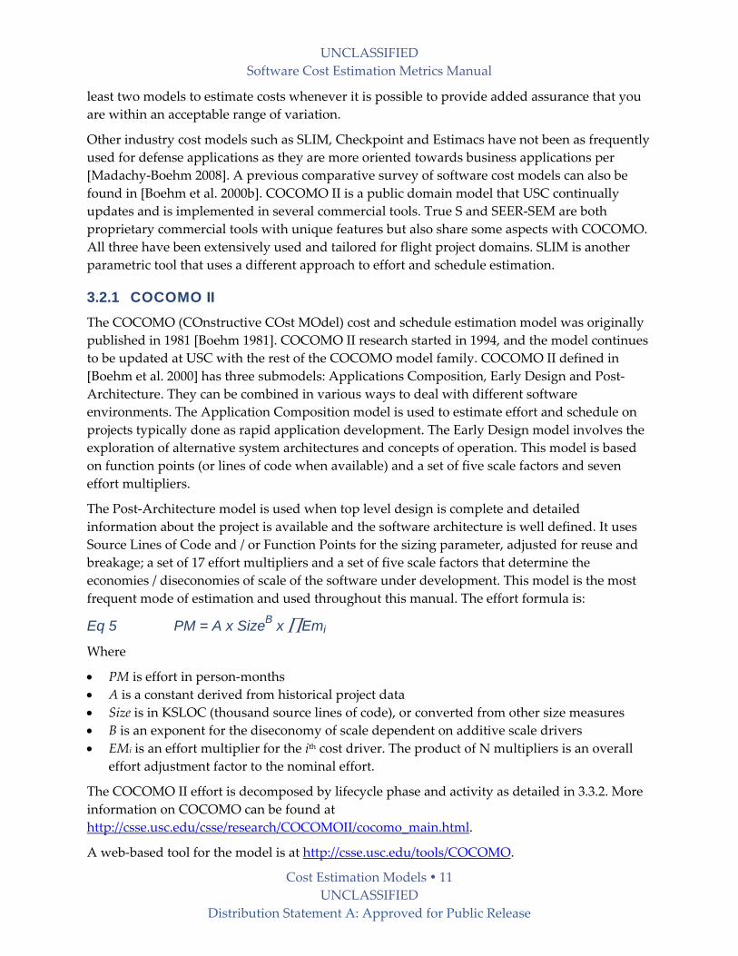
3.2.1 COCOMO II The COCOMO (COnstructive COst MOdel) cost and schedule estimation model was originally
published in 1981 [Boehm 1981]. COCOMO II research started in 1994, and the model continues
to be updated at USC with the rest of the COCOMO model family. COCOMO II defined in
[Boehm et al. 2000] has three submodels: Applications Composition, Early Design and Post‐
Architecture. They can be combined in various ways to deal with different software
environments. The Application Composition model is used to estimate effort and schedule on
projects typically done as rapid application development. The Early Design model involves the
exploration of alternative system architectures and concepts of operation. This model is based
on function points (or lines of code when available) and a set of five scale factors and seven
effort multipliers.
The Post‐Architecture model is used when top level design is complete and detailed
information about the project is available and the software architecture is well defined. It uses
Source Lines of Code and / or Function Points for the sizing parameter, adjusted for reuse and
breakage; a set of 17 effort multipliers and a set of five scale factors that determine the
economies / diseconomies of scale of the software under development. This model is the most
frequent mode of estimation and used throughout this manual. The effort formula is:
Eq 5 PM = A x SizeB x Emi
Where
PM is effort in person‐months
A is a constant derived from historical project data
Size is in KSLOC (thousand source lines of code), or converted from other size measures
B is an exponent for the diseconomy of scale dependent on additive scale drivers
EMi is an effort multiplier for the ith cost driver. The product of N multipliers is an overall
effort adjustment factor to the nominal effort.
The COCOMO II effort is decomposed by lifecycle phase and activity as detailed in 3.3.2. More
information on COCOMO can be found at
http://csse.usc.edu/csse/research/COCOMOII/cocomo_main.html.
A web‐based tool for the model is at http://csse.usc.edu/tools/COCOMO.

UNCLASSIFIED
Software Cost Estimation Metrics Manual
Cost Estimation Models 12 UNCLASSIFIED
Distribution Statement A: Approved for Public Release
3.2.2 SEER-SEM SEER‐SEM is a product offered by Galorath, Inc. This model is based on the original Jensen
model [Jensen 1983], and has been on the market over 15 years. The Jensen model derives from
COCOMO and other models in its mathematical formulation. However, its parametric
modeling equations are proprietary. Like True S, SEER‐SEM estimates can be used as part of a
composite modeling system for hardware / software systems. Descriptive material about the
model can be found in [Galorath‐Evans 2006].
The scope of the model covers all phases of the project lifecycle, from early specification
through design, development, delivery and maintenance. It handles a variety of environmental
and application configurations, and models different development methods and languages.
Development modes covered include object oriented, reuse, COTS, spiral, waterfall, prototype
and incremental development. Languages covered are 3rd and 4th generation languages (C++,
FORTRAN, COBOL, Ada, etc.), as well as application generators.
The SEER‐SEM cost model allows probability levels of estimates, constraints on staffing, effort
or schedule, and it builds estimates upon a knowledge base of existing projects. Estimate
outputs include effort, cost, schedule, staffing, and defects. Sensitivity analysis is also provided
as is a risk analysis capability. Many sizing methods are available including lines of code and
function points. For more information, see the Galorath Inc. website at
http://www.galorath.com.
3.2.3 SLIM The SLIM model is based on work done by Putnam [Putnam 1978] using the Norden / Rayleigh
manpower distribution. The central part of Putnamʹs model, called the software equation, is
[Putnam‐Myers 1992]:
Eq 6 Product = Productivity Parameter x (Effort/B)1/3 x Time4/3
Where
Product is the new and modified software lines of code at delivery time
Productivity Parameter is a process productivity factor
Effort man years of work by all job classifications
B is a special skills factor that is a function of size
Time is lapsed calendar time in years
The Productivity Parameter, obtained from calibration, has values that fall in 36 quantized steps
ranging from 754 to 3,524,578. The special skills factor, B, is a function of size in the range from
18,000 to 100,000 delivered SLOC that increases as the need for integration, testing, quality
assurance, documentation and management skills grows.
The software equation can be rearranged to estimate total effort in man years:
Eq 7 Effort = (Size x B1/3 / Productivity Parameter)3 x (1/Time4)
Putnamʹs model is used in the SLIM software tool based for cost estimation and manpower
scheduling [QSM 2003].
UNCLASSIFIED
Software Cost Estimation Metrics Manual
Cost Estimation Models 13 UNCLASSIFIED
Distribution Statement A: Approved for Public Release
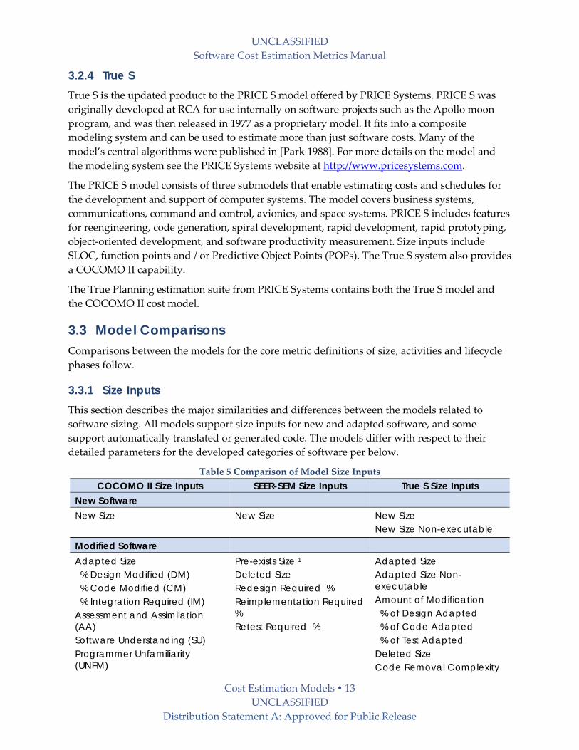
3.2.4 True S True S is the updated product to the PRICE S model offered by PRICE Systems. PRICE S was
originally developed at RCA for use internally on software projects such as the Apollo moon
program, and was then released in 1977 as a proprietary model. It fits into a composite
modeling system and can be used to estimate more than just software costs. Many of the
model’s central algorithms were published in [Park 1988]. For more details on the model and
the modeling system see the PRICE Systems website at http://www.pricesystems.com.
The PRICE S model consists of three submodels that enable estimating costs and schedules for
the development and support of computer systems. The model covers business systems,
communications, command and control, avionics, and space systems. PRICE S includes features
for reengineering, code generation, spiral development, rapid development, rapid prototyping,
object‐oriented development, and software productivity measurement. Size inputs include
SLOC, function points and / or Predictive Object Points (POPs). The True S system also provides
a COCOMO II capability.
The True Planning estimation suite from PRICE Systems contains both the True S model and
the COCOMO II cost model.
3.3 Model Comparisons Comparisons between the models for the core metric definitions of size, activities and lifecycle
phases follow.
3.3.1 Size Inputs This section describes the major similarities and differences between the models related to
software sizing. All models support size inputs for new and adapted software, and some
support automatically translated or generated code. The models differ with respect to their
detailed parameters for the developed categories of software per below.
Table 5 Comparison of Model Size Inputs
COCOMO II Size Inputs SEER-SEM Size Inputs True S Size Inputs
New Software New Size New Size New Size
New Size Non-executable
Modified Software Adapted Size % Design Modified (DM) % Code Modified (CM) % Integration Required (IM) Assessment and Assimilation (AA) Software Understanding (SU) Programmer Unfamiliarity (UNFM)
Pre-exists Size 1 Deleted Size Redesign Required % Reimplementation Required % Retest Required %
Adapted Size Adapted Size Non-executable Amount of Modification % of Design Adapted % of Code Adapted % of Test Adapted Deleted Size Code Removal Complexity
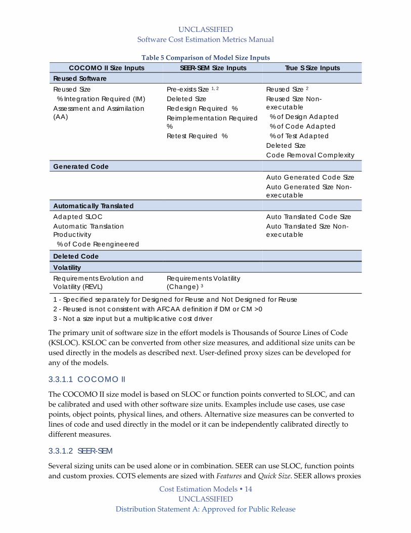
UNCLASSIFIED
Software Cost Estimation Metrics Manual
Cost Estimation Models 14 UNCLASSIFIED
Distribution Statement A: Approved for Public Release
Table 5 Comparison of Model Size Inputs
COCOMO II Size Inputs SEER-SEM Size Inputs True S Size Inputs
Reused Software Reused Size % Integration Required (IM) Assessment and Assimilation (AA)
Pre-exists Size 1, 2 Deleted Size Redesign Required % Reimplementation Required % Retest Required %
Reused Size 2 Reused Size Non-executable % of Design Adapted % of Code Adapted % of Test Adapted Deleted Size Code Removal Complexity
Generated Code Auto Generated Code Size
Auto Generated Size Non-executable
Automatically Translated Adapted SLOC Automatic Translation Productivity % of Code Reengineered
Auto Translated Code Size Auto Translated Size Non-executable
Deleted Code Volatility Requirements Evolution and Volatility (REVL)
Requirements Volatility (Change) 3
1 - Specified separately for Designed for Reuse and Not Designed for Reuse 2 - Reused is not consistent with AFCAA definition if DM or CM >0 3 - Not a size input but a multiplicative cost driver
The primary unit of software size in the effort models is Thousands of Source Lines of Code
(KSLOC). KSLOC can be converted from other size measures, and additional size units can be
used directly in the models as described next. User‐defined proxy sizes can be developed for
any of the models.
3.3.1.1 COCOMO II
The COCOMO II size model is based on SLOC or function points converted to SLOC, and can
be calibrated and used with other software size units. Examples include use cases, use case
points, object points, physical lines, and others. Alternative size measures can be converted to
lines of code and used directly in the model or it can be independently calibrated directly to
different measures.
3.3.1.2 SEER-SEM
Several sizing units can be used alone or in combination. SEER can use SLOC, function points
and custom proxies. COTS elements are sized with Features and Quick Size. SEER allows proxies

UNCLASSIFIED
Software Cost Estimation Metrics Manual
Cost Estimation Models 15 UNCLASSIFIED
Distribution Statement A: Approved for Public Release
as a flexible way to estimate software size. Any countable artifact can be established as measure.
Custom proxies can be used with other size measures in a project. Available pre‐defined proxies
that come with SEER include Web Site Development, Mark II Function Point, Function Points (for
direct IFPUG‐standard function points) and Object‐Oriented Sizing.
SEER converts all size data into internal size units, also called effort units, Sizing in SEER‐SEM
can be based on function points, source lines of code, or user‐defined metrics. Users can
combine or select a single metric for any project element or for the entire project. COTS WBS
elements also have specific size inputs defined either by Features, Object Sizing, or Quick Size,
which describe the functionality being integrated.
New Lines of Code are the original lines created for the first time from scratch.
Pre‐Existing software is that which is modified to fit into a new system. There are two categories
of pre‐existing software:
Pre‐existing, Designed for Reuse
Pre‐existing, Not Designed for Reuse.
Both categories of pre‐existing code then have the following subcategories:
Pre‐existing lines of code which is the number of lines from a previous system
Lines to be Deleted are those lines deleted from a previous system.
Redesign Required is the percentage of existing code that must be redesigned to meet new system
requirements.
Reimplementation Required is the percentage of existing code that must be re‐implemented,
physically recoded, or reentered into the system, such as code that will be translated into
another language.
Retest Required is the percentage of existing code that must be retested to ensure that it is
functioning properly in the new system.
SEER then uses different proportional weights with these parameters in their AAF equation
according to:
Eq 8 Pre-existing Effective Size = (0.4 x A) + (0.25 x B) + (0.3 5x C)
Where
A is the percentages of code redesign
B is the percentages of code reimplementation
C is the percentages of code retest required
SEER also has the capability to take alternative size inputs:

UNCLASSIFIED
Software Cost Estimation Metrics Manual
Cost Estimation Models 16 UNCLASSIFIED
Distribution Statement A: Approved for Public Release
Function-Point Based Sizing External Input (EI)
External Output (EO)
Internal Logical File (ILF)
External Interface Files (EIF)
External Inquiry (EQ)
Internal Functions (IF) ‚ any functions that are neither data nor transactions
Proxies Web Site Development
Mark II Function Points
Function Points (direct)
Object‐Oriented Sizing.
COTS Elements Quick Size
Application Type Parameter
Functionality Required Parameter
Features
Number of Features Used
Unique Functions
Data Tables Referenced
Data Tables Configured
3.3.1.3 True S
The True S software cost model size measures may be expressed in different size units
including Source Lines of Code (SLOC), function points, Predictive Object Points (POPs) or Use
Case Conversion Points (UCCPs). True S also differentiates executable from non‐executable
software sizes. Functional Size describes software size in terms of the functional requirements
that you expect a Software COTS component to satisfy. The True S software cost model size
definitions for all of the size units are listed below.
Adapted Code Size
This describes the amount of existing code that must be changed, deleted, or adapted for use
in the new software project. When the value is zero (0.00), the value for New Code Size or
Reused Code Size must be greater than zero.
Adapted Size Non‐executable
This value represents the percentage of the adapted code size that is non‐executable (such as
data statements, type declarations, and other non‐procedural statements). Typical values for
fourth generation languages range from 5.00 percent to 30.00 percent. When a value cannot
be obtained by any other means, the suggested nominal value for non‐executable code is
15.00 percent.
UNCLASSIFIED
Software Cost Estimation Metrics Manual
Cost Estimation Models 17 UNCLASSIFIED
Distribution Statement A: Approved for Public Release
Amount for Modification
This represents the percent of the component functionality that you plan to modify, if any.
The Amount for Modification value (like Glue Code Size) affects the effort calculated for the
Software Design, Code and Unit Test, Perform Software Integration and Test, and Perform
Software Qualification Test activities.
Auto Gen Size Non‐executable
This value represents the percentage of the Auto Generated Code Size that is non‐executable
(such as, data statements, type declarations, and other non‐procedural statements). Typical
values for fourth generation languages range from 5.00 percent to 30.00 percent. If a value
cannot be obtained by any other means, the suggested nominal value for non‐executable
code is 15.00 percent.
Auto Generated Code Size
This value describes the amount of code generated by an automated design tool for
inclusion in this component.
Auto Trans Size Non‐executable
This value represents the percentage of the Auto Translated Code Size that is non‐
executable (such as, data statements, type declarations, and other non‐procedural
statements). Typical values for fourth generation languages range from 5.00 percent to 30.00
percent. If a value cannot be obtained by any other means, the suggested nominal value for
non‐executable code is 15.00 percent.
Auto Translated Code Size
This value describes the amount of code translated from one programming language to
another by using an automated translation tool (for inclusion in this component).
Auto Translation Tool Efficiency
This value represents the percentage of code translation that is actually accomplished by the
tool. More efficient auto translation tools require more time to configure the tool to translate.
Less efficient tools require more time for code and unit test on code that is not translated.
Code Removal Complexity
This value describes the difficulty of deleting code from the adapted code. Two things need
to be considered when deleting code from an application or component: the amount of
functionality being removed and how tightly or loosely this functionality is coupled with
the rest of the system. Even if a large amount of functionality is being removed, if it is
accessed through a single point rather than from many points, the complexity of the
integration will be reduced.
Deleted Code Size
This describes the amount of pre‐existing code that you plan to remove from the adapted
code during the software project. The Deleted Code Size value represents code that is
included in Adapted Code Size, therefore, it must be less than, or equal to, the Adapted
Code Size value.
UNCLASSIFIED
Software Cost Estimation Metrics Manual
Cost Estimation Models 18 UNCLASSIFIED
Distribution Statement A: Approved for Public Release
Equivalent Source Lines of Code The ESLOC (Equivalent Source Lines of Code) value describes the magnitude of a selected cost
object in Equivalent Source Lines of Code size units. True S does not use ESLOC in routine
model calculations, but provides an ESLOC value for any selected cost object. Different
organizations use different formulas to calculate ESLOC.
The True S calculation for ESLOC is:
Eq 9 ESLOC = New Code + (0.7 x Adapted Code) + (0.1 x Reused Code)
To calculate ESLOC for a Software COTS, True S first converts Functional Size and Glue Code
Size inputs to SLOC using a default set of conversion rates. New Code includes Glue Code Size
and Functional Size when the value of Amount for Modification is greater than or equal to 25%.
Adapted Code includes Functional Size when the value of Amount for Modification is less than
25% and greater than zero. Reused Code includes Functional Size when the value of Amount
for Modification equals zero.
Functional Size
This value describes software size in terms of the functional requirements that you expect a
Software COTS component to satisfy. When you select Functional Size as the unit of
measure (Size Units value) to describe a Software COTS component, the Functional Size
value represents a conceptual level size that is based on the functional categories of the
software (such as Mathematical, Data Processing, or Operating System). A measure of
Functional Size can also be specified using Source Lines of Code, Function Points, Predictive
Object Points or Use Case Conversion Points if one of these is the Size Unit selected.
Glue Code Size
This value represents the amount of Glue Code that will be written. Glue Code holds the
system together, provides interfaces between Software COTS components, interprets return
codes, and translates data into the proper format. Also, Glue Code may be required to
compensate for inadequacies or errors in the COTS component selected to deliver desired
functionality.
New Code Size
This value describes the amount of entirely new code that does not reuse any design, code,
or test artifacts. When the value is zero (0.00), the value must be greater than zero for
Reused Code Size or Adapted Code Size.
New Size Non‐executable
This value describes the percentage of the New Code Size that is non‐executable (such as
data statements, type declarations, and other non‐procedural statements). Typical values for
fourth generation languages range from 5.0 percent to 30.00 percent. If a value cannot be
obtained by any other means, the suggested nominal value for non‐executable code is 15.00
percent.
Percent of Code Adapted
This represents the percentage of the adapted code that must change to enable the adapted
code to function and meet the software project requirements.

UNCLASSIFIED
Software Cost Estimation Metrics Manual
Cost Estimation Models 19 UNCLASSIFIED
Distribution Statement A: Approved for Public Release
Percent of Design Adapted
This represents the percentage of the existing (adapted code) design that must change to
enable the adapted code to function and meet the software project requirements. This value
describes the planned redesign of adapted code. Redesign includes architectural design
changes, detailed design changes, and any necessary reverse engineering.
Percent of Test Adapted
This represents the percentage of the adapted code test artifacts that must change. Test plans
and other artifacts must change to ensure that software that contains adapted code meets
the performance specifications of the Software Component cost object.
Reused Code Size
This value describes the amount of pre‐existing, functional code that requires no design or
implementation changes to function in the new software project. When the value is zero
(0.00), the value must be greater than zero for New Code Size or Adapted Code Size.
Reused Size Non‐executable
This value represents the percentage of the Reused Code Size that is non‐executable (such
as, data statements, type declarations, and other non‐procedural statements). Typical values
for fourth generation languages range from 5.00 percent to 30.00 percent. If a value cannot
be obtained by any other means, the suggested nominal value for non‐executable code is
15.00 percent.
3.3.1.4 SLIM
SLIM uses effective system size composed of new and modified code. Deleted code is not
considered in the model. If there is reused code, then the Productivity Index (PI) factor may be
adjusted to add in time and effort for regression testing and integration of the reused code.
SLIM provides different sizing techniques including:
Sizing by history
Total system mapping
Sizing by decomposition
Sizing by module
Function point sizing.
Alternative sizes to SLOC such as use cases or requirements can be used in Total System
Mapping. The user defines the method and quantitative mapping factor.
3.3.2 Lifecycles, Activities and Cost Categories COCOMO II allows effort and schedule to be allocated to either a waterfall or MBASE lifecycle.
MBASE is a modern iterative and incremental lifecycle model like the Rational Unified Process
(RUP) or the Incremental Commitment Model (ICM). The phases include: (1) Inception, (2)
Elaboration, (3) Construction, and (4) Transition.
True‐S uses the nine DoD‐STD‐2167A development phases: (1) Concept, (2) System
Requirements, (3) Software Requirements, (4) Preliminary Design, (5) Detailed Design, (6) Code
/ Unit Test, (7) Integration & Test, (8) Hardware / Software Integration, and (9) Field Test.

UNCLASSIFIED
Software Cost Estimation Metrics Manual
Cost Estimation Models 20 UNCLASSIFIED
Distribution Statement A: Approved for Public Release
In SEER‐SEM the standard lifecycle activities include: (1) System Concept, (2) System
Requirements Design, (3) Software Requirements Analysis, (4) Preliminary Design, (5) Detailed
Design, (6) Code and Unit Test, (7) Component Integration and Testing, (8) Program Test, (9)
Systems Integration through OT&E & Installation, and (10) Operation Support. Activities may
be defined differently across development organizations and mapped to SEER‐SEMs
designations.
In SLIM the lifecycle maps to four general phases of software development. The default phases
are: 1) Concept Definition, 2) Requirements and Design, 3) Construct and Test, and 4) Perfective
Maintenance. The phase names, activity descriptions and deliverables can be changed in SLIM.
The “main build” phase initially computed by SLIM includes the detailed design through
system test phases, but the model has the option to include the “requirements and design”
phase, including software requirements and preliminary design, and a “feasibility study” phase
to encompass system requirements and design.
The phases covered in the models are summarized in the Table 6.
UNCLASSIFIED
Software Cost Estimation Metrics Manual
Cost Estimation Models 21 UNCLASSIFIED
Distribution Statement A: Approved for Public Release
Table 6 Lifecycle Phase Coverage
Model Phases
COCOMO II
Inception Elaboration Construction Transition
SEER-SEM
System Concept System Requirements Design Software Requirements Analysis Preliminary Design Detailed Design Code / Unit Test Component Integration and Testing Program Test System Integration Through OT&E and Installation Operation Support
True S
Concept System Requirements Software Requirements Preliminary Design Detailed Design Code / Unit Test Integration and Test Hardware / Software Integration Field Test System Integration and Test Maintenance
SLIM
Concept Definition Requirements and Design Construction and Test Perfective Maintenance

UNCLASSIFIED
Software Cost Estimation Metrics Manual
Cost Estimation Models 22 UNCLASSIFIED
Distribution Statement A: Approved for Public Release
The work activities estimated in the respective tools are in Table 7.
Table 7 Work Activities Coverage
Model Activities
COCOMO II
Management Environment / CM Requirements Design Implementation Assessment Deployment
SEER-SEM
Management Software Requirements Design Code Data Programming Test CM QA
True S
Design Programming Data SEPGM QA CFM
SLIM
WBS Sub-elements of Phases: Concept Definition Requirements and Design Construct and Test Perfective Maintenance
The categories of labor covered in the estimation models and tools are listed in Table 8.
Table 8 Labor Activities Covered
Model Categories
COCOMO II Software Engineering Labor*
SEER-SEM Software Engineering Labor* Purchases
True S
Software Engineering Labor* Purchased Good Purchased Service Other Cost
SLIM Software Engineering Labor * Project Management (including contracts), Analysts, Designers, Programmers, Testers, CM, QA, and Documentation

UNCLASSIFIED
Software Cost Estimation Metrics Manual
Software Resource Data Report (SRDR) 23 UNCLASSIFIED
Distribution Statement A: Approved for Public Release
4 Software Resource Data Report (SRDR) The Software Resources Data Report (SRDR) is used to obtain both the estimated and actual
characteristics of new software developments or upgrades. Both the Government program
office and, after contract award, the software contractor submit this report. For contractors, this
report constitutes a contract data deliverable that formalizes the reporting of software metric
and resource data. All contractors, developing or producing any software development element
with a projected software effort greater than $20M (then year dollars) on major contracts and
subcontracts within ACAT I and ACAT IA programs, regardless of contract type, must submit
SRDRs. The data collection and reporting applies to developments and upgrades whether
performed under a commercial contract or internally by a government Central Design Activity
(CDA) under the terms of a Memorandum of Understanding (MOU).
4.1 DCARC Repository The Defense Cost and Resource Center (DCARC), which is part of OSD Cost Assessment and
Program Evaluation (CAPE), exists to collect Major Defense Acquisition Program (MDAP) cost
and software resource data and make those data available to authorized Government analysts.
Their website1 is the authoritative source of information associated with the Cost and Software
Data Reporting (CSDR) system, including but not limited to: policy and guidance, training
materials, and data. CSDRs are DoD’s only systematic mechanism for capturing completed
development and production contract ʺactualsʺ that provide the right visibility and consistency
needed to develop credible cost estimates. Since credible cost estimates enable realistic budgets,
executable contracts and program stability, CSDRs are an invaluable resource to the DoD cost
analysis community and the entire DoD acquisition community.
The Defense Cost and Resource Center (DCARC), was established in 1998 to assist in the re‐
engineering of the CSRD process. The DCARC is part of OSD Cost Assessment and Program
Evaluation (CAPE). The primary role of the DCARC is to collect current and historical Major
Defense Acquisition Program cost and software resource data in a joint service environment
and make those data available for use by authorized government analysts to estimate the cost of
ongoing and future government programs, particularly DoD weapon systems.
The DCARCʹs Defense Automated Cost Information Management System (DACIMS) is the
database for access to current and historical cost and software resource data needed to develop
independent, substantiated estimates. DACIMS is a secure website that allows DoD
government cost estimators and analysts to browse through almost 30,000 CCDRs, SRDR and
associated documents via the Internet. It is the largest repository of DoD cost information.
1 http://dcarc.cape.osd.mil/CSDR/CSDROverview.aspx

UNCLASSIFIED
Software Cost Estimation Metrics Manual
Software Resource Data Report (SRDR) 24 UNCLASSIFIED
Distribution Statement A: Approved for Public Release
4.2 SRDR Reporting Frequency The SRDR Final Developer Report contains measurement data as described in the contractorʹs
SRDR Data Dictionary. The data reflects the scope relevant to the reporting event, Table 9. Both
estimates (DD Form 2630‐1,2) and actual results (DD Form 2630‐3) of software (SW)
development efforts are reported for new or upgrade projects.
SRDR submissions for contract complete event shall reflect the entire software development
project.
When the development project is divided into multiple product builds, each representing
production level software delivered to the government, the submission should reflect each
product build.
SRDR submissions for completion of a product build shall reflect size, effort, and schedule
of that product build.
Table 9 SRDR Reporting Events
Event Report
Due Who Provides Scope of Report
Pre-Contract (180 days prior to award)
Initial Government Program Office
Estimates of the entire completed project. Measures should reflect cumulative grand totals.
Contract award
Initial Contractor Estimates of the entire project at the level of detail agreed upon. Measures should reflect cumulative grand totals.
At start of each build
Initial Contractor Estimates for completion for the build only.
Estimates corrections
Initial Contractor Corrections to the submitted estimates.
At end of each build
Final Contractor Actuals for the build only.
Contract completion
Final Contractor Actuals for the entire project. Measures should reflect cumulative grand totals.
Actuals corrections
Final Contractor Corrections to the submitted actuals.
Perhaps it is not readily apparent how important it is to understand the submission criteria.
SRDR records are a mixture of complete contracts and individual builds within a contract. And
there are initial and final reports along with corrections. Mixing contract data and build data or
mixing initial and final results or not using the latest corrected version will produce
inconclusive, if not incorrect, results.
The report consists of two pages, see Chapter 9.4. The fields in each page are listed below.

UNCLASSIFIED
Software Cost Estimation Metrics Manual
Software Resource Data Report (SRDR) 25 UNCLASSIFIED
Distribution Statement A: Approved for Public Release
4.3 SRDR Content
4.3.1 Administrative Information (SRDR Section 3.1) Security Classification
Major Program
Program Name
Phase / Milestone
Reporting Organization Type (Prime, Subcontractor, Government)
Name / Address
Reporting Organization
Division
Approved Plan Number
Customer (Direct‐Reporting Subcontractor Use Only)
Contract Type
WBS Element Code
WBS Reporting Element
Type Action
Contract No
Latest Modification
Solicitation No
Common Reference Name
Task Order / Delivery Order / Lot No
Period of Performance
Start Date (YYYYMMDD)
End Date (YYYYMMDD)
Appropriation (RDT&E, Procurement, O&M)
Submission Number
Resubmission Number
Report As Of (YYYYMMDD)
Date Prepared (YYYYMMDD)
Point of Contact
Name (Last, First, Middle Initial)
Department
Telephone Number (include Area Code)
Development Organization
Software Process Maturity
Lead Evaluator
Certification Date

UNCLASSIFIED
Software Cost Estimation Metrics Manual
Software Resource Data Report (SRDR) 26 UNCLASSIFIED
Distribution Statement A: Approved for Public Release
Evaluator Affiliation
Precedents (List up to five similar systems by the same organization or team.)
SRDR Data Dictionary Filename
Comments (on Report Context and Development Organization)
4.3.2 Product and Development Description (SRDR Section 3.2) Functional Description. A brief description of its function.
Software Development Characterization
Application Type
Primary and Secondary Programming Language.
Percent of Overall Product Size. Approximate percentage (up to 100%) of the product
size that is of this application type.
Actual Development Process. Enter the name of the development process followed for
the development of the system.
Software Development Method(s). Identify the software development method or
methods used to design and develop the software product .
Upgrade or New Development. Indicate whether the primary development was new
software or an upgrade.
Software Reuse. Identify by name and briefly describe software products reused from
prior development efforts (e.g. source code, software designs, requirements
documentation, etc.).
COTS / GOTS Applications Used.
Name. List the names of the applications or products that constitute part of the final
delivered product, whether they are COTS, GOTS, or open‐source products.
Integration Effort (Optional). If requested by the CWIPT, the SRD report shall contain
the actual effort required to integrate each COTS / GOTS application identified in
Section 3.2.4.1.
Staffing.
Peak Staff. The actual peak team size, measured in full‐time equivalent (FTE) staff.
Peak Staff Date. Enter the date when the actual peak staffing occurred.
Hours per Staff‐Month. Enter the number of direct labor hours per staff‐month.
Personnel Experience in Domain. Stratify the project staff domain experience by experience
level and specify the percentage of project staff at each experience level identified. Sample
Format 3 identifies five levels:
Very Highly Experienced (12 or more years)
Highly Experienced (6 to 12 years)
Nominally Experienced (3 to 6 years)
Low Experience (1 to 3 years)
Inexperienced / Entry Level (less than a year)

UNCLASSIFIED
Software Cost Estimation Metrics Manual
Software Resource Data Report (SRDR) 27 UNCLASSIFIED
Distribution Statement A: Approved for Public Release
4.3.3 Product Size Reporting (SRDR Section 3.3) Number of Software Requirements. Provide the actual number of software requirements.
Total Requirements. Enter the actual number of total requirements satisfied by the
developed software product at the completion of the increment or project.
New Requirements. Of the total actual number of requirements reported, identify how
many are new requirements.
Number of External Interface Requirements. Provide the number of external interface
requirements, as specified below, not under project control that the developed system
satisfies.
Total External Interface Requirements. Enter the actual number of total external interface
requirements satisfied by the developed software product at the completion of the
increment or project.
New External Interface Requirements. Of the total number of external interface
requirements reported, identify how many are new external interface requirements.
Requirements Volatility. Indicate the amount of requirements volatility encountered during
development as a percentage of requirements that changed since the Software Requirements
Review.
Software Size.
Delivered Size. Capture the delivered size of the product developed, not including any
code that was needed to assist development but was not delivered (such as temporary
stubs, test scaffoldings, or debug statements). Additionally, the code shall be partitioned
(exhaustive with no overlaps) into appropriate development categories. A common set
of software development categories is new, reused with modification, reused without
modification, carry‐over code, deleted code, and auto‐generated code.
Reused Code With Modification. When code is included that was reused with
modification, provide an assessment of the amount of redesign, recode, and retest
required to implement the modified or reused code.
Reuse Code Without Modification. Code reused without modification is code that
has no design or code modifications. However, there may be an amount of retest
required. Percentage of retest should be reported with the retest factors described
above.
Carryover Code. Report shall distinguish between code developed in previous
increments that is carried forward into the current increment and code added as part
of the effort on the current increment.
Deleted Code. Include the amount of delivered code that was created and
subsequently deleted from the final delivered code.
Auto‐generated Code. If the developed software contains auto‐generated source
code, report an auto‐generated code sizing partition as part of the set of
development categories.
Subcontractor‐Developed Code.

UNCLASSIFIED
Software Cost Estimation Metrics Manual
Software Resource Data Report (SRDR) 28 UNCLASSIFIED
Distribution Statement A: Approved for Public Release
Counting Convention. Identify the counting convention used to count software size.
Size Reporting by Programming Language (Optional).
Standardized Code Counting (Optional). If requested, the contractor shall use a publicly
available and documented code counting tool, such as the University of Southern
California Code Count tool, to obtain a set of standardized code counts that reflect
logical size. These results shall be used to report software sizing.
4.3.4 Resource and Schedule Reporting (SRDR Section 3.4)
The Final Developer Report shall contain actual schedules and actual total effort for each software development activity.
Effort. The units of measure for software development effort shall be reported in staff‐
hours. Effort shall be partitioned into discrete software development activities.
WBS Mapping.
Subcontractor Development Effort. The effort data in the SRD report shall be separated
into a minimum of two discrete categories and reported separately: Prime Contractor
Only and All Other Subcontractors.
Schedule. For each software development activity reported, provide the actual start and
end dates for that activity.
4.3.5 Product Quality Reporting (SRDR Section 3.5 - Optional) Quality should be quantified operationally (through failure rate and defect discovery rate).
However, other methods may be used if appropriately explained in the associated SRDR Data
Dictionary.
Number of Defects Discovered. Report an estimated number of defects discovered during
integration and qualification testing. If available, list the expected defect discovery counts
by priority, e.g. 1, 2, 3, 4, 5. Provide a description of the priority levels if used.
Number of Defects Removed. Report an estimated number of defects removed during
integration and qualification testing. If available, list the defect removal counts by priority.

UNCLASSIFIED
Software Cost Estimation Metrics Manual
Software Resource Data Report (SRDR) 29 UNCLASSIFIED
Distribution Statement A: Approved for Public Release
4.3.6 Data Dictionary The SRDR Data Dictionary contains, at a minimum, the following information in addition to the
specific requirements identified in Sections 3.1 through 3.5:
Experience Levels. Provide the contractorʹs specific definition (i.e., the number of years of
experience) for personnel experience levels reported in the SRD report.
Software Size Definitions. Provide the contractorʹs specific internal rules used to count
software code size.
Software Size Categories. For each software size category identified (i.e., New, Modified,
Unmodified, etc.), provide the contractorʹs specific rules and / or tools used for classifying
code into each category.
Peak Staffing. Provide a definition that describes what activities were included in peak
staffing.
Requirements Count (Internal). Provide the contractorʹs specific rules and / or tools used to
count requirements.
Requirements Count (External). Provide the contractorʹs specific rules and / or tools used to
count external interface requirements.
Requirements Volatility. Provide the contractorʹs internal definitions used for classifying
requirements volatility.
Software Development Activities. Provide the contractorʹs internal definitions of labor
categories and activities included in the SRD reportʹs software activity.
Product Quality Reporting. Provide the contractorʹs internal definitions for product quality
metrics being reported and specific rules and / or tools used to count the metrics.

UNCLASSIFIED
Software Cost Estimation Metrics Manual
Data Assessment and Processing 30 UNCLASSIFIED
Distribution Statement A: Approved for Public Release
5 Data Assessment and Processing This chapter discusses transforming the SRDR data into useful information for use in creating
Cost Estimating Relationships (CER) and to provide productivity benchmarks for use in
management oversight.
The Software Resources Data Report (SRDR) has data quality issues not uncommon with other
datasets. This presents many challenges when attempting to create CERs and productivity
benchmarks. The list below shows the challenges when working with this data:
Inadequate information on modified code (only size provided)
Inadequate information on size change or growth
Size measured inconsistently
Inadequate information on average staffing or peak staffing
Inadequate information on personnel experience
Inaccurate effort data in multi‐build components
Missing effort data
Replicated duration (start and end dates) across components
Inadequate information on schedule compression
Missing schedule data
No quality data
The remedy for some of these challenges is to find a way to normalize the data to the definitions
discussed in Chapter 2. Other techniques are required to fill in missing data, either by
consulting other sources or using statistical techniques to fill in missing values in a table. What
is needed is a process to make the data usable.
5.1 Workflow The data assessment and processing workflow has six steps. This workflow was used in the
analysis of the SRDR data. Each of these steps is described in detail.
1. Gather the data that has been collected.
2. Review and inspect each data point.
3. Determine a quantitative quality level based on the data inspection.
4. Correct missing or questionable data. There were several things that can be done about this.
Data that cannot be repaired is excluded from the analysis.
5. The data has to be normalized to a common unit of measure or scope of what is covered by
the data.
6. Finally the data is segmented by Operating Environment and Software Domain.
5.1.1 Gather Collected Data Historical data is stored in a variety of formats. Often there is data in a record that is not
relevant for cost estimation analysis. All too often, there is not enough data to support a
thorough analysis.

UNCLASSIFIED
Software Cost Estimation Metrics Manual
Data Assessment and Processing 31 UNCLASSIFIED
Distribution Statement A: Approved for Public Release
The data has to be transformed from different formats into a common data format that supports
the analysis objectives. A common data format for cost estimation analysis would be different
for analysis of requirements growth, defect discovery / removal or process improvement return
on investment to name a few.
The common data format for cost estimation analysis requires detail information on:
Amount of workload (expressed as a functional measure or a product measure)
Development and support effort
Project or build duration
Additional contextual data is needed to provide information on what the data represents, e.g.,
Organization that developed the software
What the application does
Where the software fits into the system (is it all of the software, a build, a configuration
item, or a small software unit)
The common data format used in analyzing SRDR data had additional information than was
found in the SRDR report.
5.1.2 Inspect each Data Point As the gathered data is being transformed into the common data format, inspect the data for
completeness, integrity, and “reasonable‐ness”. The first activity is to examine the project
context information.
Project Context Are all of the data available to fill the common data format fields?
How would this software component be characterized?
What does this component do?
Were there any extenuating circumstances concerning development, e.g. management
change, large requirements change, stop / restart work?
Is the Data Dictionary for that record available as a standalone file?
Is there any additional information that can be consulted about the data during analysis,
such as:
Acquisition Strategy
Acquisition Support Plan (ASP)
Contract Plan
Cost Analysis Requirements Document (CARD)
Capability Description Document (CDD)
Software Requirements Specification (SRS)
Work Breakdown Structure (WBS)
Earned Value Management System data (EVMS)
Next, the size, effort, schedule and productivity data are examined.

UNCLASSIFIED
Software Cost Estimation Metrics Manual
Data Assessment and Processing 32 UNCLASSIFIED
Distribution Statement A: Approved for Public Release
Size Data Does the size data look sound?
Is the size part of multi‐build release?
Was all code auto‐generated?
Was code rewritten after AG?
Was a portion of a legacy system included in the sizing data?
How much software was adapted (modified)?
How much software was reused (no changes)?
Is there effort and schedule data for each software activity?
Is there repeating size data?
Effort Data What labor was included in the reported hours?
Engineering labor
Management labor
Support labor: CM, QA, Process Improvement, Safety, Security, Dev. Environment
support
What labor was reported in the ʺOtherʺ activity?
Was Requirements effort reported for all builds?
Were there continuous integration activities across all builds?
Schedule Data Was there schedule compression mentioned on the project
Were there parallel multiple builds (same start & end date)
Productivity Screening Is a quick productivity check reasonably close to software with similar functionality?
Is this record an outlier in a scatter plot with other similar data?

UNCLASSIFIED
Software Cost Estimation Metrics Manual
Data Assessment and Processing 33 UNCLASSIFIED
Distribution Statement A: Approved for Public Release
5.1.3 Determine Data Quality Levels From the inspection process, assign the record a data quality rating. The criteria in Table 10 can
be used to determine rating values.
Table 10 Data Quality Rating Scale
Attribute Value Condition
Size: 1.0 if size data present 0 if no size data
Size Count Type: (providing size
data is present)
1.0 if size is Logical SLOC 0.7 if size is Non-Commented Source Statements 0.5 if size is Physical Lines (Comment and Source Statements) 0.4 if size is Total Lines (all lines in file: blank, comment, source) 0 if no size data
ESLOC Parameters:
1.0 if modification parameters provided for Auto-gen, Modified & Reuse
0.5 if New SLOC and no size data for Auto-gen, Modified or Reuse 0 if no modification parameters provided for either Modified, Auto-
gen, or Reused SLOC counts
CSCI-level Data: 1.0 if Total Size is 5,000 < Size < 250,000 0 if Total Size < 5,000 or Size > 250,000
Effort: 1.0 if effort reported for all phases 0.5 if effort is reported as a total 0 if effort is missing for a phase
Schedule: 1.0 if duration reported for all phases 0.5 if duration is reported as a total 0 is duration is missing for a phase
Productivity: 1.0 if record is in the expected value range 0.5 if record is within 1 standard deviation from the mean 0 if record is a clear outlier
As each record is rated by the criteria above, an overall quality level is assigned by:
Eq 10 Quality Level = (Size + Size Count Type + ESLOC Parameters + CSCI level + Effort + Schedule + Productivity) / 7
The quality level is a quick indicator of the degree of issues found in the record. As the recorded
is corrected through supplemental information, the rating is revised. Because the range of the
quality level scale is between 0 and 1.0, it could be used as a weight during analysis.

UNCLASSIFIED
Software Cost Estimation Metrics Manual
Data Assessment and Processing 34 UNCLASSIFIED
Distribution Statement A: Approved for Public Release
5.1.4 Correct Missing or Questionable Data The quality level makes clear which records need additional work. There are several approaches
available to resolving missing or questionable data. These are listed in a recommended order:
1. Consult the accompanying Data Dictionary discussed in Chapter 4.3.6
2. Consult any supplemental on the project that is available, e.g., ASP, CARD, CDD, EVMS,
SRS, WBS, etc.
3. Scheduling follow‐up meetings with SRDR data contributor. Data quality issues that were
fixed in the past by the SRDR contributor:
Revised missing size, effort and duration data
Obtained Adaptation Adjustment Factor (AAF) parameters
Confirmed productivity type and environment
Confirmed CSCI‐level of reporting
Asked about problems with ‐ high / low, long / short ‐ size, effort and duration data
As a result of inspecting the data and attempting to correct the issues found, no ʺbadʺ data or
“outliers” are excluded from the analysis on arbitrary grounds. However, data issues that
cannot be resolved are excluded from analysis.
5.1.5 Normalize Size and Effort Data Normalizing data is making a type of data the same. For example, if SLOC was measured by
different criteria, all SLOC counts are converted into a common count method. If effort data
covers different lifecycle phases, all effort data is converted to cover the same phases.
Normalization reduces noise in the data. Otherwise, it will pose a significant threat to statistical
validity.
5.1.5.1 Converting to Logical SLOC
With the SRDR data, the SLOC were counted using different methods.
Total Count: a line in a file, e.g. carriage returns including blanks and comment lines
Non‐Commented Source Statements (NCSS) Count: a line in a file that is not a blank or
comment line
Logical Count: as defined earlier in Chapter 2.2.2.1
For analysis, the definition of a source line of code needs to be as consistent as possible to
eliminate noise in the data. A logical source line of code has been selected as the baseline SLOC
definition.

UNCLASSIFIED
Software Cost Estimation Metrics Manual
Data Assessment and Processing 35 UNCLASSIFIED
Distribution Statement A: Approved for Public Release
If a source line of code count was defined as either Total or NCSS, these counts were converted
to a Logical SLOC count. An experiment was run using the UCC tool, described in Appendix
9.2, on public domain software applications and additional contributions from USC‐CSSE
Affiliates. Total, NCSS and Logical counts were taken from the program files. Six programming
languages were sampled:
Ada
C#
C/C++
Java
PERL
PHP
The total number of data points was 40. The results of this experiment are described next.
NCSS Line Count Conversion to Logical
The size counts for NCSS and Logical were analyzed for their relationship. Two analyses were
conducted, one for all of the size data and another for the lower 80% of the size data. The two
relationships are expressed as follows (the intercept was constrained to zero2):
Eq 11 All Sizes: Logical SLOC count = 0.44 x NCSS count
Eq 12 Lower 80%: Logical SLOC count = 0.66 x NCSS count
The statistics for these relationships are in Table 11 and a scatter plot in Figure 1.
Table 11 NCSS‐Logical Relationship Statistics
Statistics All Sizes Lower 80%
Coefficient 0.44 0.66
Total number of observations 40 32
Min - Max Range (KSLOC) 2.3 – 1,690 2.3 – 149
Adjusted R2 0.86 0.95
Standard Error 0.03 0.03
Lower 95% Confidence Interval 0.38 0.60
Upper 95% Confidence Interval 0.55 0.71
T-Statistic 15.35 23.73
2 When modeling this relationship, an overhead amount (as represented by an intercept value) does not
make sense, i.e., there is no overhead if there are zero lines to be converted. Incidentally, when the
regression was run on all sizes without the zero constraint, the constant had a T‐statistic of 1.90 and a P‐
level of 0.70.

UNCLASSIFIED
Software Cost Estimation Metrics Manual
Data Assessment and Processing 36 UNCLASSIFIED
Distribution Statement A: Approved for Public Release
All Counts Lower 80% of Counts
Figure 1 NCSS to Logical SLOC Plot
Total Line Count Conversion to Logical
As with NCSS counts, counts for NCSS and Logical were analyzed for their relationship. Two
analyses were conducted, one for all of the size data and another for the lower 80% of the size
data. The two relationships are expressed as follows (the intercept was constrained to zero):
Eq 13 All Sizes: Logical SLOC count = 0.29 x Total count
Eq 14 Lower 80%: Logical SLOC count = 0.34 x Total count
The statistics for these relationships are in Table 12 and a scatter plot in Figure 2.
Table 12 Total‐Logical Relationship Statistics
Statistics All Sizes Lower 80%
Coefficient 0.29 0.34
Total number of observations 40 32
Min - Max Range (KSLOC) 3.5 – 2,249 3.5 – 265
Adjusted R2 0.95 0.85
Standard Error 0.01 0.03
Lower 90% Confidence Interval 0.27 0.29
Upper 90% Confidence Interval 0.31 0.39
T-Statistic 27.12 13.00

UNCLASSIFIED
Software Cost Estimation Metrics Manual
Data Assessment and Processing 37 UNCLASSIFIED
Distribution Statement A: Approved for Public Release
All Counts Lower 80% of Counts
Figure 2 Total to Logical SLOC Plot
Conclusion
The 80% solution was used in this analysis. The 80% conversion factors appear to be more
“reasonable” than the 100% factors. A future version of this manual will explore the
relationships for NCSS and Total counts to Logical counts for each of the six programming
languages.
5.1.5.2 Convert Raw SLOC into Equivalent SLOC
Equivalent Size is a method used to make new and adapted code equivalent so they can be
rolled up into an aggregate size estimate (discussed in Chapter 2.3.2). This adjustment is called
Equivalent Source Lines of Code (ESLOC):
Eq 15 ESLOC = New SLOC + (AAFM x Modified SLOC) + (AAFR x Reused SLOC) + (AAFAG x Auto-Generated SLOC)
Where: AAFi = (0.4 x DM) + (0.3 x CM) + (0.3 x IM)
The SRDR data did not include the parameters for DM, CM and IM. Independent data
collection of similar data was conducted. Based on the data collected and the grouping of the
data by Operating Environment (Chapter 5.2.1) and Productivity Types (Chapter 5.2.2),
guidelines for filling‐in missing data were derived from that data that had the adaptation
parameters, Table 13.
As shown in the equation above, there are four types of code: New, Auto‐Generated, Reused,
and Modified (see Chapter 2.2.1). The DM, CM and IM parameters are not required for each
type.
New code does not require any adaption parameters. Nothing has been modified.
UNCLASSIFIED
Software Cost Estimation Metrics Manual
Data Assessment and Processing 38 UNCLASSIFIED
Distribution Statement A: Approved for Public Release
Auto‐Generated code does not require the DM or CM adaption parameters. However, it
does require testing, IM. If Auto‐Generated code does require modification, then it becomes
Modified code and the adaptation factors for Modified code apply.
Reuse code does not require the DM or CM adaption parameters either. It also requires
testing, IM. If Reused code does require modification, then it becomes Modified code and
the adaptation factors for Modified code apply.
Modified code requires the three parameters, DM, CM and IM, representing modifications
to the modified code design, code and integration testing.
Table 13 shows DM, CM and IM for different productivity types. The table shows the code type,
number of records used to derive the adaptation parameters, the mean value of the parameter
with its 95% confidence interval, and the mean value. The adaptation adjustment factor (AAF)
is shown in the last column. This factor is the portion of adapted code that will be used for
equivalent SLOC. Unfortunately there was not enough data to support reporting for all
productivity types.
Table 13 Adapted Code Parameters
DM CM IM PT Code Type # Mean M Mean M Mean M AAF Auto-Gen 0 0.00 ± 0.00 0.00 0.00
SCP Reused 18 0.51 ± 0.21 0.42 0.15 Modified 7 0.26 ± 0.22 0.25 0.33 ± 0.20 0.50 0.66 ± 0.40 1.00 0.40 Auto-Gen 0 0.00 ± 0.00 0.00 0.00
RTE Reused 8 0.17 ± 0.23 0.10 0.05 Modified 14 0.13 ± 0.10 0.05 0.30 ± 0.19 0.10 0.95 ± 0.07 1.00 0.85 Auto-Gen 1 0.13 ± 0.00 0.13 0.04
MP Reused 12 0.36 ± 0.20 0.33 0.11 Modified 21 0.75 ± 0.12 1.00 0.89 ± 0.12 1.00 0.95 ± 0.07 1.00 0.85 Auto-Gen 12 0.37 ± 0.25 0.13 0.11
SYS Reused 6 0.56 ± 0.40 0.50 0.17 Modified 14 0.22 ± 0.19 0.03 0.34 ± 0.20 0.17 0.68 ± 0.18 0.58 0.39 Auto-Gen 7 0.12 ± 0.20 0.10 0.04
SCI Reused 15 0.46 ± 0.20 0.33 0.14 Modified 10 0.34 ± 0.30 0.17 0.53 ± 0.30 0.41 0.78 ± 0.18 0.88 0.53 Auto-Gen 2 0.33 ± 0.00 0.33 0.10
IIS Reused 7 0.45 ± 0.24 0.33 0.14 Modified 4 1.00 ± 0.00 1.00 0.81 ± 0.60 1.00 0.90 ± 0.32 1.00 0.91
General observations and usage guidelines are:
The more real‐time nature of the software, the less the design is modified, i.e. Intel and
Information Systems (IIS) have a DM of 100% whereas Sensor Control and Signal Processing
(SCP) have a DM of 26%.
The same is generally true for CM. The real‐time nature appears to influence how much
code is modified.
UNCLASSIFIED
Software Cost Estimation Metrics Manual
Data Assessment and Processing 39 UNCLASSIFIED
Distribution Statement A: Approved for Public Release
IM is usually higher than either DM or CM. It the software being estimated requires more
reliability or is more complex, a higher value for IM should be used.
While the mean value is provided for DM, CM and IM, compare the mean to the median. This is
an indication of skewing in the data. This should also influence your decision on which values
to choose within the 95% confidence interval.
A future version of this manual will process more data and expand the adapted code parameter
table to additional productivity types. It will also analyze these parameters across operating
environments.
5.1.5.3 Adjust for Missing Effort Data
Guidelines for adjusting for missing effort data are shown in Table 14. As these were developed,
consideration was given to the productivity type (PT). Average Effort percentages were derived
for each Productivity Type using the analysis dataset (~300 records). Any missing effort data
was adjusted using the appropriate effort percentage and productivity type. Data missing more
than two phases of effort were not used in the analysis. This analysis is based on research by
[Tan 2012].
Table 14 Average Activity Effort Percentages Based On Complete Data
Productivity Type Requirement Arch & Design Code & Unit Test Integration & QT
IIS 11.56% 27.82% 35.63% 24.99% MP 20.56% 15.75% 28.89% 34.80% PLN 16.22% 12.27% 50.78% 20.73% RTE 15.47% 26.65% 26.71% 31.17% SCI 7.38% 39.90% 32.05% 20.67% SSP 10.80% 45.20% 20.34% 23.66% SYS 17.61% 21.10% 28.75% 32.54% VC 18.47% 23.60% 31.32% 26.61%
A future version of this manual will process more data and expand the average effort
percentages table to additional productivity types. Additionally, analysis of schedule duration
for the different activities will be conducted.
5.2 Data Segmentation Data segmentation can be challenging because Cost and Schedule Estimating Relationships
(CER and SER) are different for different types of software. Factors such as application
complexity; impact of loss due to reliability; autonomous modes of operation; constraints on
timing, storage, and power; security requirements; and complex interfaces influence the cost
and time to develop applications. Parametric cost models have a number of adjustable
parameters that attempt to account for these factors. Many of these parameters, however, are
unknown until contract award.

UNCLASSIFIED
Software Cost Estimation Metrics Manual
Data Assessment and Processing 40 UNCLASSIFIED
Distribution Statement A: Approved for Public Release
Instead of developing CERs and SERs with many parameters, the approach taken by this project
is based on grouping similar software applications together. These groups are called
Application Domains. Application Domains implement a combination of hardware and
software components to achieve the intended functionality. However, because Application
Domains then to represent an entire subsystem, e.g. Communications, the approach taken was
to use a generic description of software domains called productivity types (PT). The operating
environment for each PT is considered as well. Both the operating environment and domain are
considered in this analysis to produce the productivity types.
5.2.1 Operating Environments (OpEnv)
Operating Environments have similar systems, similar products, similar operational characteristics, and similar requirements:
High‐speed vehicle versus stationary
Battery operated versus ground power
Unrecoverable platform versus readily accessible
Limited, non‐upgradeable computing processor capacity versus racks of processors
Fixed internal and external memory capacity versus expandable capacity
There are 11 operating environments:
Table 15 Operating Environments Operating Environment (OpEnv) Examples
Ground Site (GS) Fixed (GSF) Command Post, Ground Operations Center,
Ground Terminal, Test Faculties
Mobile (GSM) Intelligence gathering stations mounted on vehicles, Mobile missile launcher
Ground Vehicle (GV) Manned (GVM) Tanks, Howitzers, Personnel carrier
Unmanned (GVU) Robotic vehicles
Maritime Vessel (MV) Manned (MVM)
Aircraft carriers, destroyers, supply ships, submarines
Unmanned (MVU) Mine hunting systems, Towed sonar array
Aerial Vehicle (AV) Manned (AVM) Fixed-wing aircraft, Helicopters Unmanned (AVU) Remotely piloted air vehicles
Space Vehicle (SV) Manned (SVM) Passenger vehicle, Cargo vehicle, Space
station
Unmanned (SVU) Orbiting satellites (weather, communications), Exploratory space vehicles
Ordinance Vehicle (OV) Unmanned (OVU) Air-to-air missiles, Air-to-ground missiles, Smart bombs, Strategic missiles

UNCLASSIFIED
Software Cost Estimation Metrics Manual
Data Assessment and Processing 41 UNCLASSIFIED
Distribution Statement A: Approved for Public Release
The operating environments can be aggregated into six high-level environments. This is useful when there is not enough data for each of the 11 environments in Table 15:
1. Ground Site (GS)
2. Ground Vehicle (GV)
3. Maritime Vessel (MV)
4. Aerial Vehicle (AV)
5. Space Vehicle (SV)
6. Ordinance Vehicle (OV)
5.2.2 Productivity Types (PT)
Productivity types are groups of application productivities that are characterized by the following:
Required software reliability
Database size ‐ if there is a large data processing and storage component to the software
application
Product complexity
Integration complexity
Real‐time operating requirements
Platform volatility, Target system volatility
Special display requirements
Development re‐hosting
Quality assurance requirements
Security requirements
Assurance requirements
Required testing level
There are 14 productivity types:

UNCLASSIFIED
Software Cost Estimation Metrics Manual
Data Assessment and Processing 42 UNCLASSIFIED
Distribution Statement A: Approved for Public Release
Table 16 Productivity Types PT Description
Sensor Control and Signal Processing (SCP)
Software that requires timing-dependent device coding to enhance, transform, filter, convert, or compress data signals. Ex.: Beam steering controller, sensor receiver / transmitter control, sensor signal processing, sensor receiver / transmitter test. Ex. of sensors: antennas, lasers, radar, sonar, acoustic, electromagnetic.
Vehicle Control (VC) Hardware & software necessary for the control of vehicle primary and secondary mechanical devices and surfaces. Ex: Digital Flight Control, Operational Flight Programs, Fly-By-Wire Flight Control System, Flight Software, Executive.
Vehicle Payload (VP) Hardware & software which controls and monitors vehicle payloads and provides communications to other vehicle subsystems and payloads. Ex: Weapons delivery and control, Fire Control, Airborne Electronic Attack subsystem controller, Stores and Self-Defense program, Mine Warfare Mission Package.
Real Time Embedded (RTE) Real-time data processing unit responsible for directing and processing sensor input / output. Ex: Devices such as Radio, Navigation, Guidance, Identification, Communication, Controls And Displays, Data Links, Safety, Target Data Extractor, Digital Measurement Receiver, Sensor Analysis, Flight Termination, Surveillance, Electronic Countermeasures, Terrain Awareness And Warning, Telemetry, Remote Control.
Mission Processing (MP) Vehicle onboard master data processing unit(s) responsible for coordinating and directing the major mission systems. Ex.: Mission Computer Processing, Avionics, Data Formatting, Air Vehicle Software, Launcher Software, Tactical Data Systems, Data Control And Distribution, Mission Processing, Emergency Systems, Launch and Recovery System, Environmental Control System, Anchoring, Mooring and Towing.
Process Control (PC) Software that manages the planning, scheduling and execution of a system based on inputs, generally sensor driven.
System Software (SYS) Layers of software that sit between the computing platform and applications. Ex: Health Management, Link 16, Information Assurance, Framework, Operating System Augmentation, Middleware, Operating Systems.
Planning Software (PLN) Provides the capability to maximize the use of the platform. The system supports all the mission requirements of the platform and may have the capability to program onboard platform systems with routing, targeting, performance, map, and Intel data.
Scientific Software (SCI) Non real time software that involves significant computations and scientific analysis. Ex: Environment Simulations, Offline Data Analysis, Vehicle Control Simulators.
Training Software (TRN) Hardware and software that are used for educational and training purposes. Ex: Onboard or Deliverable Training Equipment & Software, Computer-Based Training.

UNCLASSIFIED
Software Cost Estimation Metrics Manual
Data Assessment and Processing 43 UNCLASSIFIED
Distribution Statement A: Approved for Public Release
Table 16 Productivity Types PT Description
Telecommunications (TEL) The transmission of information, e.g. voice, data, commands, images, and video across different mediums and distances. Primarily software systems that control or manage transmitters, receivers and communications channels. Ex: switches, routers, integrated circuits, multiplexing, encryption, broadcasting, protocols, transfer modes, etc.
Software Tools (TOOL) Software that is used for analysis, design, construction, or testing of computer programs. Ex: Integrated collection of tools for most development phases of the life cycle, e.g. Rational development environment.
Test Software (TST) Hardware & Software necessary to operate and maintain systems and subsystems which are not consumed during the testing phase and are not allocated to a specific phase of testing. Ex: Onboard or Deliverable Test Equipment & Software.
Intelligence & Information Software (IIS)
An assembly of software applications that allows a properly designated authority to exercise control over the accomplishment of the mission. Humans manage a dynamic situation and respond to user-input in real time to facilitate coordination and cooperation. Ex: Battle Management, Mission Control. Also, software that manipulates, transports and stores information. Ex: Database, Data Distribution, Information Processing, Internet, Entertainment, Enterprise Services*, Enterprise Information**.
* Enterprise Information (subtype of IIS)
HW & SW needed for developing functionality or software service that are unassociated, loosely coupled units of functionality. Examples are: Enterprise service management (monitoring, fault management), Machine-to-machine messaging, Service discovery, People and device discovery, Metadata discovery, Mediation, Service security, Content discovery and delivery, Federated search, Enterprise catalog service, Data source integration, Enterprise content delivery network (caching specification, distributed caching, forward staging), Session management,, Audio & video over internet protocol, Text collaboration (chat, instant messaging), Collaboration (white boarding & annotation), Application broadcasting and sharing, Virtual spaces, Identity management (people and device discovery), User profiling and customization.
** Enterprise Information (subtype of IIS)
HW & SW needed for assessing and tailoring COTS software applications or modules that can be attributed to a specific software service or bundle of services. Examples of enterprise information systems include but not limited to: , Enterprise resource planning, Enterprise data warehouse, Data mart, Operational data store. Examples of business / functional areas include but not limited to: General ledger, Accounts payable, Revenue and accounts receivable, Funds control and budgetary accounting, Cost management, Financial reporting, Real property inventory and management.
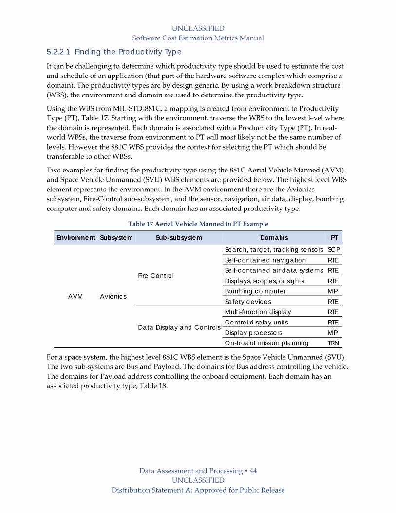
UNCLASSIFIED
Software Cost Estimation Metrics Manual
Data Assessment and Processing 44 UNCLASSIFIED
Distribution Statement A: Approved for Public Release
5.2.2.1 Finding the Productivity Type
It can be challenging to determine which productivity type should be used to estimate the cost
and schedule of an application (that part of the hardware‐software complex which comprise a
domain). The productivity types are by design generic. By using a work breakdown structure
(WBS), the environment and domain are used to determine the productivity type.
Using the WBS from MIL‐STD‐881C, a mapping is created from environment to Productivity
Type (PT), Table 17. Starting with the environment, traverse the WBS to the lowest level where
the domain is represented. Each domain is associated with a Productivity Type (PT). In real‐
world WBSs, the traverse from environment to PT will most likely not be the same number of
levels. However the 881C WBS provides the context for selecting the PT which should be
transferable to other WBSs.
Two examples for finding the productivity type using the 881C Aerial Vehicle Manned (AVM)
and Space Vehicle Unmanned (SVU) WBS elements are provided below. The highest level WBS
element represents the environment. In the AVM environment there are the Avionics
subsystem, Fire‐Control sub‐subsystem, and the sensor, navigation, air data, display, bombing
computer and safety domains. Each domain has an associated productivity type.
Table 17 Aerial Vehicle Manned to PT Example
Environment Subsystem Sub-subsystem Domains PT
AVM Avionics
Fire Control
Search, target, tracking sensors SCP Self-contained navigation RTE Self-contained air data systems RTE Displays, scopes, or sights RTE Bombing computer MP Safety devices RTE
Data Display and Controls
Multi-function display RTE Control display units RTE Display processors MP On-board mission planning TRN
For a space system, the highest level 881C WBS element is the Space Vehicle Unmanned (SVU).
The two sub‐systems are Bus and Payload. The domains for Bus address controlling the vehicle.
The domains for Payload address controlling the onboard equipment. Each domain has an
associated productivity type, Table 18.
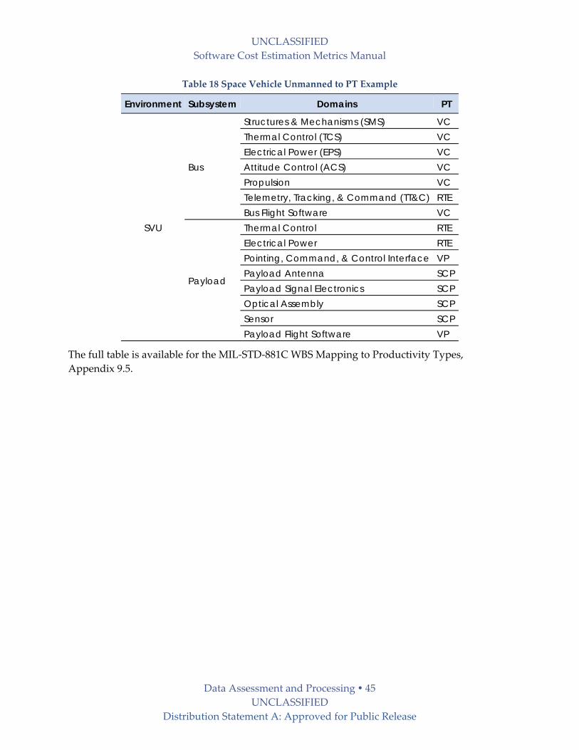
UNCLASSIFIED
Software Cost Estimation Metrics Manual
Data Assessment and Processing 45 UNCLASSIFIED
Distribution Statement A: Approved for Public Release
Table 18 Space Vehicle Unmanned to PT Example
Environment Subsystem Domains PT
SVU
Bus
Structures & Mechanisms (SMS) VC Thermal Control (TCS) VC Electrical Power (EPS) VC Attitude Control (ACS) VC Propulsion VC Telemetry, Tracking, & Command (TT&C) RTE Bus Flight Software VC
Payload
Thermal Control RTE Electrical Power RTE Pointing, Command, & Control Interface VP Payload Antenna SCP Payload Signal Electronics SCP Optical Assembly SCP Sensor SCP Payload Flight Software VP
The full table is available for the MIL‐STD‐881C WBS Mapping to Productivity Types,
Appendix 9.5.
UNCLASSIFIED
Software Cost Estimation Metrics Manual
Cost Estimating Relationship Analysis 46 UNCLASSIFIED
Distribution Statement A: Approved for Public Release
6 Cost Estimating Relationship Analysis This chapter discusses using the assessed and process SRDR data to create Cost Estimating
Relationships (CER). These relationships are different for different types of software. Factors
such as application complexity, impact of loss due to reliability, autonomous modes of
operation, constraints on timing, storage and power, security requirements, and complex
interfaces influence the cost and time to develop applications. Parametric cost models have a
number of adjustable parameters that attempt to account for these factors.
6.1 Application Domain Decomposition Instead of developing CERs and SERs with many parameters, this chapter describes an analysis
approach based on grouping similar software applications together. These groups are called
Application Domains. Application Domains implement a combination of hardware and
software components to achieve the intended functionality. Instead of using a domain name
such as Communications, a better approach is to use a generic software Productivity Type (PT).
Also consideration needs to be given to the operating environment that the domain operates
within. Both the operating environment and PT are considered in this analysis to produce CERs.
Domain analysis of the SRDR database is presented in the next sections, and provides guidance
in developing estimates in the respective domains. Cost and schedule estimating relationships
are expressed in different forms. In this manual, they are expressed as a ratio commonly called
Productivity and as a simple math equation called a Model.
6.2 SRDR Metric Definitions The SRDR was discussed in Chapter 4. In Chapter 5 the metrics were discussed for measuring
size, effort and schedule.
6.2.1 Software Size The SRDR data contained a mixture of different code count types. The data in Chapter 5.1.5.1
was used to convert all counts to the logical count type.
For pre‐existing code (Auto‐Generated, Modified and Reused), if the adaptation parameters
were not provided with the data, the guidelines in Chapter 5.1.5.2 were used.
6.2.2 Software Development Activities and Durations Software CERs have a breadth and a depth. The breadth is the number of lifecycle activities
covered and the depth is the type of labor counted in or across each activity. The activity data in
the SRDR is reported following the [ISO 12207] processes for software development. Table 19
shows the 12207 processes and the ones covered by SRDR data. This is the breadth of the CERs
reported in this manual.

UNCLASSIFIED
Software Cost Estimation Metrics Manual
Cost Estimating Relationship Analysis 47 UNCLASSIFIED
Distribution Statement A: Approved for Public Release
Table 19 ISO/IEC 12207 Development Activities
System requirements analysis System architectural design
Act
iviti
es in
SRD
R da
ta
Software requirements analysis Software architectural design Software detailed design Software coding and testing Software integration Software qualification testing
System integration System qualification testing Software installation Software acceptance support
Table 20 shows the different labor categories in the SRDR data. Not all of the records had all of
the categories. However, the Software Engineering and Assessment categories were reported
for in each record. Table 14 in Chapter 5.1.5.3 provides a distribution of effort across these
activities.
Table 20 SRDR Labor Categories
Category SRDR Labor Categories
Management Engineering Management Business Management
Software Engineering
Software Requirements Analysis Architecture and Detailed Design Coding and Unit Testing Test and Integration
Assessment Qualification Testing Development Test Evaluation Support
Support
Software Configuration Management Software Quality Assurance Configuration Audit Development Environment Support Tools Support Documentation Data Preparation Process Management Metrics Training IT Support / Data Center
When comparing results of the CER analysis with other available CER data, it is important to
keep in mind the breadth and depth of activities covered. They should be as similar as possible.
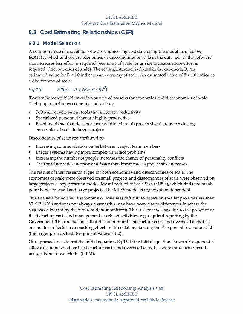
UNCLASSIFIED
Software Cost Estimation Metrics Manual
Cost Estimating Relationship Analysis 48 UNCLASSIFIED
Distribution Statement A: Approved for Public Release
6.3 Cost Estimating Relationships (CER)
6.3.1 Model Selection A common issue in modeling software engineering cost data using the model form below,
EQ(15) is whether there are economies or diseconomies of scale in the data, i.e., as the software
size increases less effort is required (economy of scale) or as size increases more effort is
required (diseconomies of scale). The scaling influence is found in the exponent, B. An
estimated value for B < 1.0 indicates an economy of scale. An estimated value of B > 1.0 indicates
a diseconomy of scale.
Eq 16 Effort = A x (KESLOCB)
[Banker‐Kemerer 1989] provide a survey of reasons for economies and diseconomies of scale.
Their paper attributes economies of scale to:
Software development tools that increase productivity
Specialized personnel that are highly productive
Fixed overhead that does not increase directly with project size thereby producing
economies of scale in larger projects
Diseconomies of scale are attributed to:
Increasing communication paths between project team members
Larger systems having more complex interface problems
Increasing the number of people increases the chance of personality conflicts
Overhead activities increase at a faster than linear rate as project size increases
The results of their research argue for both economies and diseconomies of scale. The
economies of scale were observed on small projects and diseconomies of scale were observed on
large projects. They present a model, Most Productive Scale Size (MPSS), which finds the break
point between small and large projects. The MPSS model is organization dependent.
Our analysis found that diseconomy of scale was difficult to detect on smaller projects (less than
50 KESLOC) and was not always absent (this may have been due to differences in where the
cost was allocated by the different data submitters). This, we believe, was due to the presence of
fixed start‐up costs and management overhead activities, e.g. required reporting by the
Government. The conclusion is that the amount of fixed start‐up costs and overhead activities
on smaller projects has a masking effect on direct labor; skewing the B‐exponent to a value < 1.0
(the larger projects had B‐exponent values > 1.0).
Our approach was to test the initial equation, Eq 16. If the initial equation shows a B‐exponent <
1.0, we examine whether fixed start‐up costs and overhead activities were influencing results
using a Non Linear Model (NLM):

UNCLASSIFIED
Software Cost Estimation Metrics Manual
Cost Estimating Relationship Analysis 49 UNCLASSIFIED
Distribution Statement A: Approved for Public Release
Eq 17 Effort (PM) = C + (A x KESLOCB)
Or
Eq 18 Effort (PM) = C + (KESLOCB)
Where
Effort is Person Months
C is the fixed start‐up and overhead activity costs in Person‐Months
B is a scaling factor expressing the degree of the diseconomy of scale
If the NLM shows a B‐exponent > 1.0, then the NLM is chosen. This model unmasks the
influence of fixed start‐up costs in a separate variable from the diseconomies of scale present in
the data.
A statistic that is not available for NLMs is R2, the Coefficient of Determination, used to describe
how well a regression fits a set of data. This is due to not being able to use regression analysis to
derive the NLM. Iterative search techniques are used instead. When a NLM is displayed, the R2
is displayed with the marker ***.
6.3.2 Model-Based CERs Coverage The coverage of model‐based CERs by operating environment and productivity type, discussed
in Chapters 5.2.1 and 5.2.2 respectively, are shown in Table 21. The operating environments are
the table columns. The productivity types are the rows. Not all productivity types and
environments were covered due to lack of enough data in each group (at least 5 records are
required).
The shaded cells in Table 21 denote a CER and the number in a cell is the number of records
used to create the CER. The “ALL” column and row mean for all operating environments or
productivity types.

UNCLASSIFIED
Software Cost Estimation Metrics Manual
Cost Estimating Relationship Analysis 50 UNCLASSIFIED
Distribution Statement A: Approved for Public Release
Table 21 CER Coverage
Ground
Site Ground Vehicle
Maritime Vessel
Aerial Vehicle
Space Vehicle Ordinance ALL
SCP 13 8 36 VC VP 16 16 RTE 22 9 52 MP 6 31 48 PC SYS 28 60 PLN SCI 24 39 TRN TEL TOOL TST IIS 23 37 ALL
6.3.3 Software CERs by OpEnv
6.3.3.1 Ground Site (GS) Operating Environment
Mission Processing
Eq 19 PMGSF-MP = 3.20 + (KESLOC1.19
)
Number of observations: 6
Adjusted R2: ***3
Maximum Absolute Deviation: 0.24
PRED (30): 0.83
Minimum KESLOC Value: 15
Maximum KESLOC Value: 91
3 R2 is not available for NLMs.

UNCLASSIFIED
Software Cost Estimation Metrics Manual
Cost Estimating Relationship Analysis 51 UNCLASSIFIED
Distribution Statement A: Approved for Public Release
System Software
Eq 20 PMGSF-SYS = 20.86 + (2.35 x KESLOC1.12
)
Number of observations: 28
Adjusted R2: ***
Maximum Absolute Deviation: 0.19
PRED (30): 0.82
Minimum KESLOC Value: 5
Maximum KESLOC Value: 215
Scientific Systems
Eq 21 PMGSF-SCI = 34.26 + (KESLOC1.29
)
Number of observations: 24
Adjusted R2: ****
Maximum Absolute Deviation: 0.37
PRED (30): 0.56
Minimum KESLOC Value: 5
Maximum KESLOC Value: 171
Intelligence and Information Systems
Eq 22 PMGSF-IIS = 30.83 + (1.38 x KESLOC1.13
)
Number of observations: 23
Adjusted R2: ***
Maximum Absolute Deviation: 0.16
PRED (30): 0.91
Minimum KESLOC Value: 15
Maximum KESLOC Value: 180
6.3.3.2 Ground Vehicle (GV) Operating Environment
Sensor Control and Processing
Eq 23 PMGV-SCP = 135.5 + (KESLOC1.60
)
Number of observations: 13
Adjusted R2: ***
Maximum Absolute Deviation: 0.39
PRED (30): 0.31
Minimum KESLOC Value: 1
Maximum KESLOC Value: 76

UNCLASSIFIED
Software Cost Estimation Metrics Manual
Cost Estimating Relationship Analysis 52 UNCLASSIFIED
Distribution Statement A: Approved for Public Release
Real Time Embedded
Eq 24 PMGV-RTE = 84.42 + (KESLOC1.45
)
Number of observations: 22
Adjusted R2: ***
Maximum Absolute Deviation: 0.24
PRED (30): 0.73
Minimum KESLOC Value: 9
Maximum KESLOC Value: 89
6.3.3.3 Aerial Vehicle (AV) Operating Environment
Sensor Control and Signal Processing (SCP)
Eq 25 PMAVM-SCP = 115.8 + (KESLOC1.61
)
Number of observations: 8 Adjusted R2: ***
Maximum Absolute Deviation: 0.27 PRED (30): 0.62 Minimum KESLOC Value: 6 Maximum KESLOC Value: 162
Real Time Embedded (RTE)
Eq 26 PMAVM-RTE = 5.61 x (KESLOC1.16
)
Number of observations: 9 Adjusted R2: 0.89 Maximum Absolute Deviation: 0.50 PRED (30): 0.33 Minimum KESLOC Value: 1 Maximum KESLOC Value: 167
Mission Processing (MP)
Eq 27 PMAVM-MP = 3.1 x (KESLOC1.43
)
Number of observations: 31
Adjusted R2: 0.88
Maximum Absolute Deviation: 0.50
PRED (30): 0.59
Minimum KESLOC Value: 1
Maximum KESLOC Value: 207

UNCLASSIFIED
Software Cost Estimation Metrics Manual
Cost Estimating Relationship Analysis 53 UNCLASSIFIED
Distribution Statement A: Approved for Public Release
6.3.3.4 Space Vehicle Unmanned (SVU) Operating Environment
Vehicle Payload
Eq 28 PMSV-VP = 3.15 x (KESLOC1.38
)
Number of observations: 16
Adjusted R2: 0.86
Maximum Absolute Deviation: 0.27
PRED (30): 0.50
Minimum KESLOC Value: 5
Maximum KESLOC Value: 120
6.3.4 Software CERs by PT Across All Environments The following environments were included in this analysis:
Ground Sites
Ground Vehicles
Maritime Vessels
Aerial Vehicle
Ordnance
Space Vehicle
Sensor Control and Signal Processing
Eq 29 PMAll-SCP = 74.37 + (KESLOC1.71
)
Number of observations: 36
Adjusted R2: ***
Maximum Absolute Deviation: 0.69
PRED (30): 0.31
Minimum KESLOC Value: 1
Maximum KESLOC Value: 162
Vehicle Payload
Eq 30 PMAll-VP = 3.15 + (KESLOC1.38
)
Number of observations: 16
Adjusted R2: ***
Maximum Absolute Deviation: 0.27
PRED (30): 0.50
Minimum KESLOC Value: 5
Maximum KESLOC Value: 120

UNCLASSIFIED
Software Cost Estimation Metrics Manual
Cost Estimating Relationship Analysis 54 UNCLASSIFIED
Distribution Statement A: Approved for Public Release
Real Time Embedded
Eq 31 PMAll-RTE = 34.32 + (KESLOC1.52
)
Number of observations: 52
Adjusted R2: ***
Maximum Absolute Deviation: 0.61
PRED (30): 0.46
Minimum KESLOC Value: 1
Maximum KESLOC Value: 167
Mission Processing
Eq 32 PMAll-MP = 3.48 x (KESLOC1.17
)
Number of observations: 48
Adjusted R2: 0.88
Maximum Absolute Deviation: 0.49
PRED (30): 0.58
Minimum KESLOC Value: 1
Maximum KESLOC Value: 207
System Software
Eq 33 PMAll-SYS = 16.01 + (KESLOC1.37
)
Number of observations: 60
Adjusted R2: ***
Maximum Absolute Deviation: 0.37
PRED (30): 0.53
Minimum KESLOC Value: 2
Maximum KESLOC Value: 215
Scientific Software
Eq 34 PMAll-SCI = 21.09 + (KESLOC1.36
)
Number of observations: 39
Adjusted R2: ***
Maximum Absolute Deviation: 0.65
PRED (30): 0.18
Minimum KESLOC Value: 1
Maximum KESLOC Value: 171

UNCLASSIFIED
Software Cost Estimation Metrics Manual
Cost Estimating Relationship Analysis 55 UNCLASSIFIED
Distribution Statement A: Approved for Public Release
Intelligence and Information Systems
Eq 35 PMAll-IIS = 1.27 x (KESLOC1.18
)
Number of observations: 37
Adjusted R2: 0.90
Maximum Absolute Deviation: 0.35
PRED (30): 0.65
Minimum KESLOC Value: 1
Maximum KESLOC Value: 180
Future version of this manual will show CER scatter plots, 95% confidence intervals, as well as
expand the number of CERs for productivity types and operating environments.

UNCLASSIFIED
Software Cost Estimation Metrics Manual
Cost Estimating Relationship Analysis 56 UNCLASSIFIED
Distribution Statement A: Approved for Public Release
6.4 Productivity Benchmarks
6.4.1 Model Selection and Coverage Software productivity refers to the ability of an organization to generate outputs using the
resources that it currently has as inputs. Inputs typically include facilities, people, experience,
processes, equipment, and tools. Outputs generated include software applications and
documentation used to describe them.
Eq 36 Productivity = Outputs / Inputs = KESLOC / PM
The metric used to express software productivity is Thousands of Equivalent Source Lines of
Code (KESLOC) per Person‐Month (PM) of effort. While many other measures exist, KESLOC /
PM will be used because most of the data collected by the DoD on past projects is captured
using these two measures. While controversy exists over whether or not KESLOC / PM is a
good measure, consistent use of this metric (see Metric Definitions) provides for meaningful
comparisons of productivity.
Table 22 Productivity Benchmark Coverage GSF MVM AVM SVU OVU ALL
SCP 13 7 6 38 VC VP RTE 23 6 9 53 MP 6 7 31 47 PC SYS 28 23 60 PLN SCI 23 15 39 TRN TEL TOOL TST IIS 23 35 ALL 116 67 50 6 16
The numbers in Table 22 are the number of records analyzed. The ALL column and row are not
necessarily the sum of the corresponding columns or rows. A minimum of five or more projects
were required to derive a productivity benchmark.

UNCLASSIFIED
Software Cost Estimation Metrics Manual
Cost Estimating Relationship Analysis 57 UNCLASSIFIED
Distribution Statement A: Approved for Public Release
6.4.2 Data Transformation An Anderson‐Darling test of the productivity data revealed a non‐ normal distribution. A
histogram with a gamma distribution overlay visually shows this phenomenon, left plot in
Figure 3. A Box‐Cox transformation of the productivity data showed that if the data were
transformed to log values, the distribution was much closer to a normal distribution, right plot
in Figure 3.
Figure 3 Productivity Data Distribution
This observation required the testing of each data group’s distribution for normality. Some
groups required different types of transformation and some did not require any transformation
at all. The results of the distribution testing are provided in Appendix 9.6.1, Normality Tests on
Productivity Data.
Table 24, Table 25, and Table 26 below show the productivity benchmark results. Results shown
in italics indicate the analysis was performed on transformed data. This is important to note
because statistics of data dispersion are only valid on normal distributions, i.e., they only apply
in the transformed number space. However, dispersion statistics in the transformed number
space do not provide much insight when converted back into linear number space, e.g.,
dispersion statistics in log number space are much closer together and conversion back into
linear number space results in a false measure of dispersion. Therefore the results in these tables
are reported in linear number space.
The mean value of the transformed data is valid in linear number space and can be compared to
other mean values. The dispersion statistics for the transformed statistics are, strictly speaking,
only an indicator of dispersion. The standard deviation, on which the dispersion statistics rely,
was derived manually in linear number space.
The transformations performed on each dataset and the statistical summaries are provided in
Appendices 9.6.1 and 9.6.2.
7506004503001500
50
40
30
20
10
0
Productivity
Fre
qu
en
cy
Shape 2.005
Scale 100.8N 272
Histogram of ProductivityGamma
7.26.45.64.84.03.22.4
35
30
25
20
15
10
5
0
Ln(Productivity)
Fre
qu
en
cy
Shape 35.95
Scale 0.1402N 272
Histogram of Ln(Productivity)Gamma

UNCLASSIFIED
Software Cost Estimation Metrics Manual
Cost Estimating Relationship Analysis 58 UNCLASSIFIED
Distribution Statement A: Approved for Public Release
6.4.3 Productivity Benchmark Statistics The tables of productivity results have a number of columns that are defined in Table 23.
Table 23 Productivity Statistics
Column Label Description N Number of records Min KESLOC Minimum value in thousands of equivalent source lines of code Max KESLOC Maximum value in thousands of equivalent source lines of code LCI Lower Confidence Interval is an estimate of an interval below the sample
mean within which the population mean is estimated to lie Mean Estimated sample value representing the population central value; equal to
the sum of the values divided by the number of values , i.e., arithmetic mean UCI Upper Confidence Interval is an estimate of an interval above the sample
mean within which the population mean is estimated to lie Std Dev Standard Deviation is a measure of dispersion about the mean CV Coefficient of Variation shows the extent of variability in relation to the mean of
the sample. It is defined as the ratio of the standard deviation to the mean. Q1 Numerical value for the lower 25% of ranked data (1st Quartile), i.e., the value
half way between the lowest value and the median in a set of ranked values Median Numerical value separating the higher half of a sample from the lower half, i.e.,
the middle value in a set of ranked values Q3 Numerical value for the lower 75% of ranked data (3rd Quartile), i.e. the value
half way between the median and the highest value in a set of ranked values
6.4.4 Software Productivity Benchmark Results by Operating Environment Table 24 shows the mean and median productivity across operating environments (OpEnv),
discussed in Chapter 5.2.1. To be included in the table, there had to be five or more records in
an environment group. The rows are sorted on the mean productivity from lowest to highest.
Table 24 Productivity Benchmarks by Operating Environment
OpEnv N Min
KESLOC Max
KESLOC LCI Mean UCI Std Dev CV Q1 Median Q3
SVU 6 5 134 50 85 120 44 52% 52 76 125 OVU 16 0.3 189 88 133 177 90 68% 51 120 226
AVM 50 0.32 208 108 133 158 91 68% 81 129 184
MVM 67 2 54 159 203 247 184 91% 112 193 717
GSF 116 0.61 215 182 205 227 123 60% 118 229 301
Note: Results shown in italics indicate the analysis was performed on transformed data. See
discussion in 6.3.2.
Using the median values in Table 24, Figure 4 shows a comparison of the productivities across
operating environments.

UNCLASSIFIED
Software Cost Estimation Metrics Manual
Cost Estimating Relationship Analysis 59 UNCLASSIFIED
Distribution Statement A: Approved for Public Release
Figure 4 OpEnv Median Productivities Boxplot
6.4.5 Software Productivity Benchmarks Results by Productivity Type Table 25 shows the mean and median productivity across Productivity Types (PT), discussed in
Chapter 5.2.2. To be included in the table, there had to be five or more records in a productivity
type group. The rows are sorted on the mean productivity from lowest to highest.
Table 25 Productivity Benchmarks by Productivity Type
PT N Min
KESLOC Max
KESLOC LCI Mean UCI Std Dev CV Q1 Median Q3
SCP 38 0.35 162 44 50 56 19 39% 33 53 67 RTE 53 1 167 100 120 140 75 62% 83 124 168 MP 47 1 45 135 167 199 113 68% 124 159 236 SYS 60 2 215 205 225 245 78 35% 172 219 274 SCI 39 0.32 171 200 237 275 120 51% 106 248 313 IIS 35 3 150 342 397 453 167 42% 305 363 541
Note: Results shown in italics indicate the analysis was performed on transformed data. See
discussion in 6.3.2.
Using the median values in Table 25, Figure 5 shows a comparison of the productivities across
operating environments.
SVUOVUMVMGSFAVM
800
700
600
500
400
300
200
100
0
OpEnv
PrBoxplot of Operating Environment Median Productivities

UNCLASSIFIED
Software Cost Estimation Metrics Manual
Cost Estimating Relationship Analysis 60 UNCLASSIFIED
Distribution Statement A: Approved for Public Release
Figure 5 PT Median Productivities Boxplot
SYSSCPSCIRTEMPIIS
900
800
700
600
500
400
300
200
100
0
PT
PrBoxplot of Productivity Type Median Productivities

UNCLASSIFIED
Software Cost Estimation Metrics Manual
Cost Estimating Relationship Analysis 61 UNCLASSIFIED
Distribution Statement A: Approved for Public Release
6.4.6 Software Productivity Benchmarks by OpEnv and PT Table 26 shows the mean and median productivity by operating environment (OpEnv) and
productivity type (PT). To be included in the table, there had to be five or more records in a
productivity type group. The rows are sorted on the mean productivity from lowest to highest
in each OpEnv grouping.
Table 26 Productivity Benchmarks by Operating Environment and Productivity Type
OpEnv PT N Min
KESLOC Max
KESLOC LCI Mean UCI Std Dev CV Q1 Median Q3
AVM SCP 8 6 162 47 56 65 13 23% 46 58 68 AVM RTE 9 1.5 167 69 122 174 80 66% 81 89 237 AVM MP 31 1.25 207 123 154 186 90 58% 122 141 188 GSF SCP 13 0.61 76 49 58 67 17 29% 44 60 67 GSF RTE 23 9.4 89 110 129 147 45 35% 99 130 149 GSF MP 6 14.5 91 120 162 203 52 32% 126 158 199 GSF SYS 28 5.1 215 217 240 264 64 26% 199 245 274 GSF SCI 23 4.5 171 230 271 312 99 37% 201 274 313 GSF IIS 23 15.2 180 341 376 410 85 23% 305 359 436
MVM SCP 7 5.99 24 25 39 53 19 50% 24 33 46 MVM RTE 6 2.21 38 -13 113 239 158 139% 62 110 247 MVM SCI 15 2 54 119 185 251 131 71% 55 170 327 MVM MP 7 4.931 13 150 189 228 52 28% 136 217 241 MVM SYS 23 2.05 47 199 234 269 86 37% 184 226 324 OVU RTE 11 1.2 116 96 141 410 76 54% 56 127 192
Note: Results shown in italics indicate the analysis was performed on transformed data. See
discussion in 6.3.2.
6.5 Future Work Productivity is not only influenced by the operating environment and productivity type but
also by application size. The larger the application being developed, the larger the number of
overhead activities required to coordinate the development. In general, productivity decreases
as size increases as discussed previously in Section 6.3.1.
For this reason, within an environment and PT, different productivities should be broken out
for different size groups:
0‐25 KESLOC
26‐50 KESLOC
51‐100 KESLOC
100+ KESLOC
A future version of this manual will use additional data to examine productivity changes within an operating environment and productivity type.

UNCLASSIFIED
Software Cost Estimation Metrics Manual
Modern Estimation Challenges 62 UNCLASSIFIED
Distribution Statement A: Approved for Public Release
7 Modern Estimation Challenges Several future trends will present significant future challenges for the sizing and cost estimation
of 21st century software systems. Prominent among these trends are:
Rapid change, emergent requirements, and evolutionary development
Net‐centric systems of systems
Model‐Driven and Non‐Developmental Item (NDI)‐intensive systems
Ultrahigh software system assurance
Legacy maintenance and brownfield development
Agile and Kanban development
This chapter summarizes each trend and elaborates on its challenges for software sizing and
cost estimation.
7.1 Changing Objectives, Constraints and Priorities
7.1.1 Rapid Change, Emergent Requirements, and Evolutionary Development 21st century software systems will encounter increasingly rapid change in their objectives,
constraints, and priorities. This change will be necessary due to increasingly rapid changes in
their competitive threats, technology, organizations, leadership priorities, and environments. It
is thus increasingly infeasible to provide precise size and cost estimates if the systems’
requirements are emergent rather than pre‐specifiable. This has led to increasing use of
strategies such as incremental and evolutionary development, and to experiences with
associated new sizing and costing phenomena such as the Incremental Development
Productivity Decline. It also implies that measuring the system’s size by counting the number
of source lines of code (SLOC) in the delivered system may be an underestimate, as a good deal
of software may be developed and deleted before delivery due to changing priorities.
There are three primary options for handling these sizing and estimation challenges. The first is
to improve the ability to estimate requirements volatility during development via improved
data collection and analysis, such as the use of code counters able to count numbers of SLOC
added, modified, and deleted during development [Nguyen 2010]. If such data is unavailable,
the best one can do is to estimate ranges of requirements volatility. For uniformity, Table 27
presents a recommended set of Requirements Volatility (RVOL) ranges over the development
period for rating levels of 1 (Very Low) to 5 (Very High), such as in the DoD SRDR form
[DCARC 2005].
Table 27 Recommended RVOL Rating Levels
Rating Level RVOL Range RVOL Average 1. Very Low 0-6% 3% 2. Low 6-12% 9% 3. Nominal 12-24% 18% 4. High 24-48% 36% 5. Very High >48% 72%

UNCLASSIFIED
Software Cost Estimation Metrics Manual
Modern Estimation Challenges 63 UNCLASSIFIED
Distribution Statement A: Approved for Public Release
For incremental and evolutionary development projects, the second option is to treat the earlier
increments as reused software, and to apply reuse factors to them (such as the percent of the
design, code, and integration modified, perhaps adjusted for degree of software
understandability and programmer unfamiliarity [Boehm et al. 2000]). This can be done either
uniformly across the set of previous increments, of by having these factors vary by previous
increment or by subsystem. This will produce an equivalent‐SLOC (ESLOC) size for the effect of
modifying the previous increments, to be added to the size of the new increment in estimating
effort for the new increment. In tracking the size of the overall system, it is important to
remember that these ESLOC are not actual lines of code to be included in the size of the next
release.
The third option is to include an Incremental Development Productivity Decline (IDPD) factor,
or perhaps multiple factors varying by increment or subsystem. Unlike hardware, where unit
costs tend to decrease with added production volume, the unit costs of later software
increments tend to increase, due to previous‐increment breakage and usage feedback, and due
to increased integration and test effort. Thus, using hardware‐driven or traditional software‐
driven estimation methods for later increments will lead to underestimates and overruns in
both cost and schedule.
A relevant example was a large defense software system that had the following characteristics:
5 builds, 7 years, $100M
Build 1 productivity over 300 SLOC / person‐month
Build 5 productivity under 150 SLOC / person‐month
Including Build 1‐4 breakage, integration, rework
318% change in requirements across all builds
A factor‐of‐2 decrease in productivity across four new builds corresponds to an average build‐
to‐build IDPD factor of 19%. A recent quantitative IDPD analysis of a smaller software system
yielded an IDPD of 14%, with significant variations from increment to increment [Tan et al.
2009]. Similar IDPD phenomena have been found for large commercial software such as the
multi‐year slippages in the delivery of Microsoft’s Word for Windows [Gill‐Iansiti 1994] and
Windows Vista, and for large agile‐development projects that assumed a zero IDPD factor
[Elssamadisy‐Schalliol 2002].
Based on experience with similar projects, the following impact causes and ranges per
increment are conservatively stated in Table 28:
Table 28 IDPD Effort Drivers
Less effort due to more experienced personnel, assuming reasonable initial experience level
Variation depending on personnel turnover rates 5-20% More effort due to code base growth
Breakage, maintenance of full code base 20-40% Diseconomies of scale in development, integration 10-25% Requirements volatility, user requests 10-25%
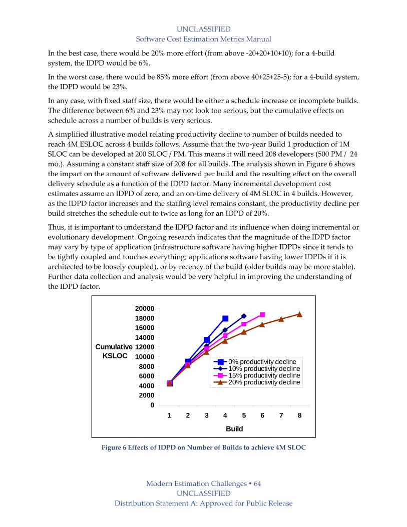
UNCLASSIFIED
Software Cost Estimation Metrics Manual
Modern Estimation Challenges 64 UNCLASSIFIED
Distribution Statement A: Approved for Public Release
In the best case, there would be 20% more effort (from above ‐20+20+10+10); for a 4‐build
system, the IDPD would be 6%.
In the worst case, there would be 85% more effort (from above 40+25+25‐5); for a 4‐build system,
the IDPD would be 23%.
In any case, with fixed staff size, there would be either a schedule increase or incomplete builds.
The difference between 6% and 23% may not look too serious, but the cumulative effects on
schedule across a number of builds is very serious.
A simplified illustrative model relating productivity decline to number of builds needed to
reach 4M ESLOC across 4 builds follows. Assume that the two‐year Build 1 production of 1M
SLOC can be developed at 200 SLOC / PM. This means it will need 208 developers (500 PM / 24
mo.). Assuming a constant staff size of 208 for all builds. The analysis shown in Figure 6 shows
the impact on the amount of software delivered per build and the resulting effect on the overall
delivery schedule as a function of the IDPD factor. Many incremental development cost
estimates assume an IDPD of zero, and an on‐time delivery of 4M SLOC in 4 builds. However,
as the IDPD factor increases and the staffing level remains constant, the productivity decline per
build stretches the schedule out to twice as long for an IDPD of 20%.
Thus, it is important to understand the IDPD factor and its influence when doing incremental or
evolutionary development. Ongoing research indicates that the magnitude of the IDPD factor
may vary by type of application (infrastructure software having higher IDPDs since it tends to
be tightly coupled and touches everything; applications software having lower IDPDs if it is
architected to be loosely coupled), or by recency of the build (older builds may be more stable).
Further data collection and analysis would be very helpful in improving the understanding of
the IDPD factor.
Figure 6 Effects of IDPD on Number of Builds to achieve 4M SLOC
0
20004000
60008000
10000
1200014000
1600018000
20000
1 2 3 4 5 6 7 8
Build
Cumulative KSLOC
0% productivity decline10% productivity decline15% productivity decline20% productivity decline

UNCLASSIFIED
Software Cost Estimation Metrics Manual
Modern Estimation Challenges 65 UNCLASSIFIED
Distribution Statement A: Approved for Public Release
CBA Growth Trend in USC e-Services Projects
0
10
20
30
40
50
60
70
80
1997 1998 1999 2000 2001 2002
Year
Per
cen
tag
e Faʹ06 ‐
Spʹ07
19%
Faʹ07 ‐
Spʹ08,
35%
Faʹ08 ‐
Spʹ09,
50%
Faʹ09 ‐
Spʹ10,
57%
Percentage
Year
7.1.2 Net-centric Systems of Systems (NCSoS) If one is developing software components for use in a NCSoS, changes in the interfaces between
the component systems and independently‐evolving NCSoS‐internal or NCSoS‐external
systems will add further effort. The amount of effort may vary by the tightness of the coupling
among the systems; the complexity, dynamism, and compatibility of purpose of the
independently‐evolving systems; and the degree of control that the NCSoS protagonist has over
the various component systems. The latter ranges from Directed SoS (strong control), through
Acknowledged (partial control) and Collaborative (shared interests) SoSs , to Virtual SoSs (no
guarantees) [USD(AT&L) 2008].
For estimation, one option is to use requirements volatility as a way to assess increased effort.
Another is to use existing models such as COSYSMO [Valerdi 2008] to estimate the added
coordination effort across the NCSoS [Lane 2009]. A third approach is to have separate models
for estimating the systems engineering, NCSoS component systems development, and NCSoS
component systems integration to estimate the added effort [Lane‐Boehm 2007].
7.1.3 Model-Driven and Non-Developmental Item (NDI)-Intensive Development Model‐driven development and Non‐Developmental Item (NDI)‐intensive development are
two approaches that enable large portions of software‐intensive systems to be generated from
model directives or provided by NDIs such as Commercial‐Off‐The‐Shelf (COTS) components,
open source components, and purchased services such as Cloud services. Figure 7 shows recent
trends in the growth of COTS‐Based Applications (CBAs) [Yang et al. 2005] and services‐
intensive systems [Koolmanojwong‐Boehm 2010] in the area of web‐based e‐services.
Figure 7 COTS and Services‐Intensive Systems Growth in USC E‐Services Projects
Such applications are highly cost‐effective, but present several sizing and cost estimation
challenges:
Model directives generate source code in Java, C++, or other third‐generation languages, but
unless the generated SLOC are going to be used for system maintenance, their size as
counted by code counters should not be used for development or maintenance cost
estimation.

UNCLASSIFIED
Software Cost Estimation Metrics Manual
Modern Estimation Challenges 66 UNCLASSIFIED
Distribution Statement A: Approved for Public Release
Counting model directives is possible for some types of model‐driven development, but
presents significant challenges for others (e.g., GUI builders).
Except for customer‐furnished or open‐source software that is expected to be modified, the
size of NDI components should not be used for estimating.
A significant challenge is to find appropriately effective size measures for such NDI
components. One approach is to use the number and complexity of their interfaces with
each other or with the software being developed. Another is to count the amount of glue‐
code SLOC being developed to integrate the NDI components, with the proviso that such
glue code tends to be about 3 times as expensive per SLOC as regularly‐developed code
[Basili‐Boehm, 2001]. A similar approach is to use the interface elements of function points
for sizing [Galorath‐Evans 2006].
A further challenge is that much of the effort in using NDI is expended in assessing
candidate NDI components and in tailoring them to the given application. Some initial
guidelines for estimating such effort are provided in the COCOTS model [Abts 2004]. •
Another challenge is that the effects of COTS and Cloud‐services evolution are generally
underestimated during software maintenance. COTS products generally provide significant
new releases on the average of about every 10 months, and generally become unsupported
after three new releases. With Cloud services, one does not have the option to decline new
releases, and updates occur more frequently. One way to estimate this source of effort is to
consider it as a form of requirements volatility.
Another serious concern is that functional size measures such as function points, use cases,
or requirements will be highly unreliable until it is known how much of the functionality is
going to be provided by NDI components or Cloud services.
7.1.4 Ultrahigh Software Systems Assurance The increasing criticality of software to the safety of transportation vehicles, medical equipment,
or financial resources; the security of private or confidential information; and the assurance of
“24 / 7” Internet, web, or Cloud services will require further investments in the development
and certification of software than are provided by most current software‐intensive systems.
While it is widely held that ultrahigh‐assurance software will substantially raise software–
project cost, different models vary in estimating the added cost. For example, [Bisignani‐Reed
1988] estimates that engineering highly–secure software will increase costs by a factor of 8; the
1990’s Softcost‐R model estimates a factor of 3.43 [Reifer 2002]; the SEER model uses a similar
value of 3.47 [Galorath‐Evans 2006].
A recent experimental extension of the COCOMO II model called COSECMO used the 7
Evaluated Assurance Levels (EALs) in the ISO Standard Common Criteria for Information
Technology Security Evaluation (CC) [ISO 1999], and quoted prices for certifying various EAL
security levels to provide an initial estimation model in this context [Colbert‐Boehm 2008]. Its
added‐effort estimates were a function of both EAL level and software size: its multipliers for a
5000‐SLOC secure system were 1.50 for EAL 4 and 8.8 for EAL 7.
A further sizing challenge for ultrahigh‐assurance software is that it requires more functionality
for such functions as security audit, communication, cryptographic support, data protection,

UNCLASSIFIED
Software Cost Estimation Metrics Manual
Modern Estimation Challenges 67 UNCLASSIFIED
Distribution Statement A: Approved for Public Release
etc. These may be furnished by NDI components or may need to be developed for special
systems.
7.1.5 Legacy Maintenance and Brownfield Development Fewer and fewer software‐intensive systems have the luxury of starting with a clean sheet of
paper or whiteboard on which to create a new Greenfield system. Most software‐intensive
systems are already in maintenance; [Booch 2009] estimates that there are roughly 200 billion
SLOC in service worldwide. Also, most new applications need to consider continuity of service
from the legacy system(s) they are replacing. Many such applications involving incremental
development have failed because there was no way to separate out the incremental legacy
system capabilities that were being replaced. Thus, such applications need to use a Brownfield
development approach that concurrently architect the new version and its increments, while re‐
engineering the legacy software to accommodate the incremental phase‐in of the new
capabilities [Hopkins‐Jenkins 2008; Lewis et al. 2008; Boehm 2009].
Traditional software maintenance sizing models have determined an equivalent SLOC size by
multiplying the size of the legacy system by its Annual Change Traffic (ACT) fraction (% of
SLOC added + % of SLOC modified) / 100. The resulting equivalent size is used to determine a
nominal cost of a year of maintenance, which is then adjusted by maintenance‐oriented effort
multipliers. These are generally similar or the same as those for development, except for some,
such as required reliability and degree of documentation, in which larger development
investments will yield relative maintenance savings. Some models such as SEER [Galorath‐
Evans 2006] include further maintenance parameters such as personnel and environment
differences. An excellent summary of software maintenance estimation is in [Stutzke 2005].
However, as legacy systems become larger and larger (a full‐up BMW contains roughly 100
million SLOC [Broy 2010]), the ACT approach becomes less stable. The difference between an
ACT of 1% and an ACT of 2% when applied to 100 million SLOC is 1 million SLOC. A recent
revision of the COCOMO II software maintenance model sizes a new release as ESLOC =
2*(Modified SLOC) + Added SLOC + 0.5* (Deleted SLOC). The coefficients are rounded values
determined from the analysis of data from 24 maintenance activities [Nguyen, 2010], in which
the modified, added, and deleted SLOC were obtained from a code counting tool. This model
can also be used to estimate the equivalent size of re‐engineering legacy software in Brownfield
software development. At first, the estimates of legacy SLOC modified, added, and deleted will
be very rough, and can be refined as the design of the maintenance modifications or Brownfield
re‐engineering is determined.

UNCLASSIFIED
Software Cost Estimation Metrics Manual
Modern Estimation Challenges 68 UNCLASSIFIED
Distribution Statement A: Approved for Public Release
7.1.6 Agile and Kanban Development The difficulties of software maintenance estimation can often be mitigated by using workflow
management techniques such as Kanban [Anderson 2010]. In Kanban, individual maintenance
upgrades are given Kanban cards (Kanban is the Japanese word for card; the approach
originated with the Toyota Production System). Workflow management is accomplished by
limiting the number of cards introduced into the development process, and pulling the cards
into the next stage of development (design, code, test, release) when open capacity is available
(each stage has a limit of the number of cards it can be processing at a given time). Any
buildups of upgrade queues waiting to be pulled forward are given management attention to
find and fix bottleneck root causes or to rebalance the manpower devoted to each stage of
development. A key Kanban principle is to minimize work in progress.
An advantage of Kanban is that if upgrade requests are relatively small and uniform, that there
is no need to estimate their required effort; they are pulled through the stages as capacity is
available, and if the capacities of the stages are well‐tuned to the traffic, work gets done on
schedule. However, if a too‐large upgrade is introduced into the system, it is likely to introduce
delays as it progresses through the stages. Thus, some form of estimation is necessary to
determine right‐size upgrade units, but it does not have to be precise as long as the workflow
management pulls the upgrade through the stages. For familiar systems, performers will be able
to right‐size the units. For Kanban in less‐familiar systems, and for sizing builds in agile
methods such as Scrum, group consensus techniques such as Planning Poker [Cohn 2005] or
Wideband Delphi [Boehm 1981]can generally serve this purpose.
The key point here is to recognize that estimation of knowledge work can never be perfect, and
to create development approaches that compensate for variations in estimation accuracy.
Kanban is one such; another is the agile methods’ approach of timeboxing or schedule‐as‐
independent‐variable (SAIV), in which maintenance upgrades or incremental development
features are prioritized, and the increment architected to enable dropping of features to meet a
fixed delivery date (With Kanban, prioritization occurs in determining which of a backlog of
desired upgrade features gets the next card). Such prioritization is a form of value‐based
software engineering, in that the higher‐priority features can be flowed more rapidly through
Kanban stages [Anderson 2010], or in general given more attention in defect detection and
removal via value‐based inspections or testing [Boehm‐Lee 2005; Li‐Boehm 2010]. Another
important point is that the ability to compensate for rough estimates does not mean that data on
project performance does not need to be collected and analyzed. It is even more important as a
sound source of continuous improvement and change adaptability efforts.
7.1.7 Putting It All Together at the Large-Project or Enterprise Level The biggest challenge of all is that the six challenges above need to be addressed concurrently.
Suboptimizing on individual‐project agility runs the risks of easiest‐first lock‐in to unscalable or
unsecurable systems, or of producing numerous incompatible stovepipe applications.
Suboptimizing on security assurance and certification runs the risks of missing early‐adopter
market windows, of rapidly responding to competitive threats, or of creating inflexible, user‐
unfriendly systems.

UNCLASSIFIED
Software Cost Estimation Metrics Manual
Modern Estimation Challenges 69 UNCLASSIFIED
Distribution Statement A: Approved for Public Release
One key strategy for addressing such estimation and performance challenges is to recognize
that large systems and enterprises are composed of subsystems that have different need
priorities and can be handled by different estimation and performance approaches. Real‐time,
safety‐critical control systems and security kernels need high assurance, but are relatively
stable. GUIs need rapid adaptability to change, but with GUI‐builder systems, can largely
compensate for lower assurance levels via rapid fixes. A key point here is that for most
enterprises and large systems, there is no one‐size‐fits‐all method of sizing, estimating, and
performing.
7.2 Estimation Approaches for Different Processes This implies a need for guidance on what kind of process to use for what kind of system or
subsystem, and on what kinds of sizing and estimation capabilities fit what kinds of processes.
A start toward such guidance is provided in Tables 3.3 and 3.4 in [Boehm‐Lane 2010].
Figure 8 summarizes the traditional single‐step waterfall process plus several forms of
incremental development, each of which meets different competitive challenges and which are
best served by different cost estimation approaches. The time phasing of each form is expressed
in terms of the increment 1, 2, 3, … content with respect to the Rational Unified Process (RUP)
phases of Inception (I), Elaboration (E), Construction (C), and Transition (T):
Figure 8 Summary of Different Processes

UNCLASSIFIED
Software Cost Estimation Metrics Manual
Modern Estimation Challenges 70 UNCLASSIFIED
Distribution Statement A: Approved for Public Release
The Single Step model is the traditional waterfall model, in which the requirements are pre‐
specified, and the system is developed to the requirements in a single increment. Single‐
increment parametric estimation models, complemented by expert judgment, are best for this
process.
The Pre‐specified Sequential incremental development model is not evolutionary. It just splits
up the development in order to field an early Initial Operational Capability, followed by several
Pre‐Planned Product Improvements (P3Is). When requirements are pre‐specifiable and stable, it
enables a strong, predictable process. When requirements are emergent and / or rapidly
changing, it often requires very expensive rework when it needs to undo architectural
commitments. Cost estimation can be performed by sequential application of single‐step
parametric models plus the use of an IDPD factor, or by parametric model extensions
supporting the estimation of increments, including options for increment overlap and breakage
of existing increments, such as the extension of COCOMO II Incremental Development Model
(COINCOMO) extension described in Appendix B of [Boehm et al. 2000].
The Evolutionary Sequential model rapidly develops an initial operational capability and
upgrades it based on operational experience. Pure agile software development fits this model: if
something is wrong, it will be fixed in 30 days in the next release. Rapid fielding also fits this
model for larger or hardware‐software systems. Its strength is getting quick‐response
capabilities in the field. For pure agile, it can fall prey to an easiest‐first set of architectural
commitments which break when, for example, it tries to add security or scalability as a new
feature in a later increment. For rapid fielding, it may be expensive to keep the development
team together while waiting for usage feedback, but it may be worth it. For small agile projects,
group consensus techniques such as Planning Poker are best; for larger projects, parametric
models with an IDPD factor are best.
Evolutionary Overlapped covers the special case of deferring the next increment until critical
enablers such as desired new technology, anticipated new commercial product capabilities, or
needed funding become available or mature enough to be added.
Evolutionary Concurrent has the systems engineers handling the change traffic and re‐
baselining the plans and specifications for the next increment, while keeping the development
stabilized for the current increment. Its example and pros and cons are provided in Table 29.

UNCLASSIFIED
Software Cost Estimation Metrics Manual
Modern Estimation Challenges 71 UNCLASSIFIED
Distribution Statement A: Approved for Public Release
Table 29 Situation‐Dependent Processes and Estimation Approaches
Type Examples Pros Cons Cost Estimation Single Step Stable; High
Assurance Pre-specifiable full-capability requirements
Emergent requirements or rapid change
Single-increment parametric estimation models
Pre-specified Sequential
Platform base plus PPPIs
Pre-specifiable full-capability requirements
Emergent requirements or rapid change
COINCOMO or repeated single-increment parametric model estimation with IDPD
Evolutionary Sequential
Small: Agile Large: Evolutionary Development
Adaptability to change
Easiest-first; late, costly breakage
Small: Planning-poker-type Large: Parametric with IDPD and Requirements Volatility
Evolutionary Overlapped
COTS-intensive systems
Immaturity risk avoidance
Delay may be noncompetitive
Parametric with IDPD and Requirements Volatility
Evolutionary Concurrent
Mainstream product lines; Systems of systems
High assurance with rapid change
Highly coupled systems with very rapid change
COINCOMO with IDPD for development; COSYSMO for re-baselining
All Cost Estimation approaches also include an expert‐judgment cross‐check.
Table 30 provides criteria for deciding which of the five classes of incremental and evolutionary
acquisition (EvA) defined in Table 29 to use, plus the choice of non‐incremental, single‐step
development.
The Single‐Step‐to‐Full‐Capability process exemplified by the traditional waterfall or sequential
Vee model is appropriate if the product’s requirements are pre‐specifiable and have a low
probability of significant change; and if there is no value in or opportunity to deliver a partial
product capability. A good example would be the hardware portion of a geosynchronous
satellite.
The Pre‐specified Sequential process is best if the product’s requirements are pre‐specifiable
and have a low probability of significant change; and if waiting for the full system to be
developed incurs a loss of important and deliverable incremental mission capabilities. A good
example would be a well‐understood and well‐prioritized sequence of software upgrades to a
programmable radio.
The Evolutionary Sequential process is best when there is a need to get operational feedback on
a quick‐response capability before defining and developing the next increment’s content. Agile
methods fit into this category, as do systems undergoing rapid competitive change.
The Evolutionary Overlapped process is best when one does not need to wait for operational
feedback, but may need to wait for next‐increment enablers such as technology maturity,
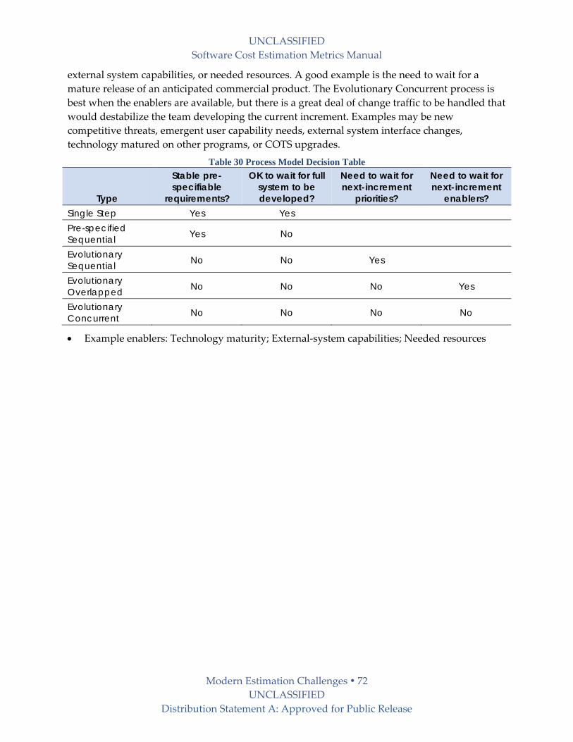
UNCLASSIFIED
Software Cost Estimation Metrics Manual
Modern Estimation Challenges 72 UNCLASSIFIED
Distribution Statement A: Approved for Public Release
external system capabilities, or needed resources. A good example is the need to wait for a
mature release of an anticipated commercial product. The Evolutionary Concurrent process is
best when the enablers are available, but there is a great deal of change traffic to be handled that
would destabilize the team developing the current increment. Examples may be new
competitive threats, emergent user capability needs, external system interface changes,
technology matured on other programs, or COTS upgrades.
Table 30 Process Model Decision Table
Type
Stable pre-specifiable
requirements?
OK to wait for full system to be developed?
Need to wait for next-increment
priorities?
Need to wait for next-increment
enablers? Single Step Yes Yes Pre-specified Sequential Yes No
Evolutionary Sequential No No Yes
Evolutionary Overlapped No No No Yes
Evolutionary Concurrent No No No No
Example enablers: Technology maturity; External‐system capabilities; Needed resources

UNCLASSIFIED
Software Cost Estimation Metrics Manual
Conclusions and Next Steps 73 UNCLASSIFIED
Distribution Statement A: Approved for Public Release
8 Conclusions and Next Steps There are two conclusions that can be drawn from the results presented in Chapter 6 Cost
Estimating Relationship Analysis:
1. The results do not provide enough certainty to be useful. In which case the reader may be
advised to be cautious of any productivity metrics.
2. The results have validity but more investigation is needed into the variability of the data and
analysis of additional data is needed as well.
This manual is still a work in progress. There are more SRDR records to be analyzed. With more
data, the results presented would be expanded and refined. The list below presents an overview
of the next steps:
Expand the SLOC count type conversions for each of the six programming languages.
Expand the adapted code parameter table to additional productivity types and operating
environments.
Expand the average effort percentages table, Table 14, to additional productivity types.
Analysis of schedule duration for the different activities will be conducted.
Expand the number of CERs for each productivity types and operating environments.
Increase the coverage of the productivity benchmarks for each operating environment and
productivity type.
Segment the productivity benchmarks by software size groups.
There are two additional chapters that should be in this manual:
1. Software Code Growth
This is a very important topic as it will impact the sensitivities of a CER‐based estimate.
2. Software Maintenance CERs and Productivity Benchmarks
With the super‐large base of DoD software, maintenance cost estimations are another
important topic.

UNCLASSIFIED
Software Cost Estimation Metrics Manual
Appendices 74 UNCLASSIFIED
Distribution Statement A: Approved for Public Release
9 Appendices
9.1 Acronyms 4GL Fourth Generation Language
AAF Adaptation Adjustment Factor: It is used with adapted software to
produce an equivalent size. It includes the effects of Design
Modified (DM), Code Modified (CM), and Integration Modified
(IM).
AAM Adaptation Adjustment Multiplier
ACAT Acquisition Category
ACEIT Automated Cost Estimating Integrated Tools
ACWP Actual Cost of Work Performed
AMS Acquisition Management System
ASP Acquisition Support Plan
AV Aerial Vehicle
AVM Aerial Vehicle Manned, e.g., Fixed‐wing aircraft, Helicopters
AVU Aerial Vehicle Unmanned, e.g., Remotely piloted air vehicles
BCWP Budgeted Cost of Work Performed
BCWS Budgeted Cost of Work Scheduled
BFP Basic Feature Point
C/SCSC Costs / Schedule Control System Criteria
CAPE Cost Assessment and Program Evaluation (an OSD organization)
CARD Cost Analysis Requirements Document
CDA Central Design Authority
CDD Capability Description Document
CDR Critical Design Review
CDRL Contract Data Requirements List
CER Cost Estimating Relationship
CER Cost Estimating Relationship
CM Code Modified Percentage
CMM Capability Maturity Model

UNCLASSIFIED
Software Cost Estimation Metrics Manual
Appendices 75 UNCLASSIFIED
Distribution Statement A: Approved for Public Release
CO Contracting Officer
COCOMO COnstructive COst MOdel
COCOTS COnstructive COTS
COTS Commercial‐off‐the Shelf
CPM Critical Path Method
CSC Computer Software Component
CSCI Computer Software Configuration Item
CSDR Cost and Software Data Report
CSU Computer Software Unit
DACIMS Defense Automated Cost Information Management System
DCARC Defense Cost and Resource Center
DDE Dynamic Data Exchange
DM Design Modified Percentage
DoD Department of Defense
EA Evolutionary Acquisition
EI External Inputs
EIF External Interfaces
EO External Outputs
EQ External Inquiries
EVMS Earned Value Management System
FAA CEH FAA Cost Estimating Handbook
FAA PH FAA Pricing Handbook
FAQ Frequently Asked Questions
FCA Functional Configuration Audit
FPA Function Point Analysis
FPC Function Point Count
FPH FAA Pricing Handbook
GAO U.S. General Accounting Office
GS Ground Site
GSF Ground Site Fixed, e.g., Command Post, Ground Operations
Center, Ground Terminal, Test Faculties

UNCLASSIFIED
Software Cost Estimation Metrics Manual
Appendices 76 UNCLASSIFIED
Distribution Statement A: Approved for Public Release
GSM Ground Site Mobile, e.g., Intelligence gathering stations mounted
on vehicles, Mobile missile launcher
GUI Graphical User Interface
GV Ground Vehicle
GVM Ground Vehicle Manned, e.g., Tanks, Howitzers, Personnel carrier
GVU Ground Vehicle Unmanned, e.g., Robot vehicles
HOL Higher Order Language
HWCI Hardware Configuration item
IDPD Incremental Development Productivity Decline
ICE Independent Cost Estimate
IEEE Institute of Electrical and Electronics Engineers
IFPUG International Function Point Userʹs Group
IIS Intelligence and Information Software
ILF Internal Files
IM Integration Modified Percentage
IRS Interface Requirement Specification
IS Information System
KDSI Thousands of Delivered Source Instructions
LCC Life Cycle Cost
MDAP Major Defense Acquisition Program
MOU Memorandum of Understanding
MPSS Most Productive Scale Size
MTTD Mean‐Time‐To‐Detect
MP Mission Processing
MSLOC Millions of source lines of code
MV Maritime Vessel
MVM Maritime Vessel Manned, e.g., Aircraft carriers, destroyers, supply
ships, submarines
MVU Maritime Vessel Unmanned, e.g., Mine hunting systems, Towed
sonar array
NASA National Aeronautics and Space Administration
NCCA Naval Center for Cost Analysis

UNCLASSIFIED
Software Cost Estimation Metrics Manual
Appendices 77 UNCLASSIFIED
Distribution Statement A: Approved for Public Release
NDI Non‐Development Item
NLM Non‐Linear Model
NRaD United States Navy’s Naval Command, Control, Surveillance
Center, RDT&E Division, Software Engineering Process Office
OO Object Oriented
OpEnv Operating Environment
OSD Office of the Secretary of Defense
OV Ordinance Vehicle
OVU Ordinance Vehicle Unmanned, e.g., Air‐to‐air missiles, Air‐to‐
ground missiles, Smart bombs, Strategic missiles
PCA Physical Configuration Audit
PERT Program Evaluation and Review Technique
PC Process Control
PLN Planning software
Pr Productivity
PT Productivity Type
RTE Real‐Time Embedded
RUP Rational Unified Process
SAIV Schedule As an Independent Variable
SCI Scientific software
SCP Sensor Control and Signal Processing (SCP)
SDD Software Design Document
SDP Software Development Plan
SDR Software Design Review
SEER A tool suite produced by Galorath
SEER‐SEM System Evaluation and Estimation of Resources Software
Estimating Model
SEI Software Engineering Institute
SER Schedule Estimating Relationship
SLIM A tool suite produced by Quantitative Software Management
SLIM Software Life Cycle Model
SLOC Source Lines of Code
UNCLASSIFIED
Software Cost Estimation Metrics Manual
Appendices 78 UNCLASSIFIED
Distribution Statement A: Approved for Public Release
SRDR Software Resource Data Report
SRR Systems Requirements Review
SRS Software Requirements Specification
SSCAG Space Systems Cost Analysis Group
SSR Software Specification Review
SSS System Segment Specification
SU Software Understanding
SV Space Vehicle
SVM Space Vehicle Manned, e.g., Passenger vehicle, Cargo vehicle,
Space station
SVU Space Vehicle Unmanned, e.g., Orbiting satellites (weather,
communications), Exploratory space vehicles
SYS System Software
TEL Telecommunications software
TOOL Software Tools
TST Test software
TRN Training Software
UCC Universal Code Counter
UNFM Programmer Unfamiliarity
USC University of Southern California
VC Vehicle Control
VP Vehicle Payload
WBS Work Breakdown Structure

UNCLASSIFIED
Software Cost Estimation Metrics Manual
Appendices 79 UNCLASSIFIED
Distribution Statement A: Approved for Public Release
9.2 Automated Code Counting Unified Code Count is a source code counting and differencing tool. It allows the user to count,
compare, and collect both physical and logical differentials between two versions of the source
code of a software product. The differencing capabilities allow users to count the number of
added / new, deleted, modified, and unmodified physical and logical source lines of code
(SLOC) of the current version in comparison with the previous version. With the counting
capabilities, users can generate the physical, non‐commented source statements, logical SLOC
counts, and other sizing information, such as comment and keyword counts, of the target
program. The tool can be compiled using a C/C++ supported compiler. It is run by providing
files of filenames to be counted or providing the directories where the files reside. It can be
downloaded free from the USC Center for Systems and Software Engineering4.
Figure 9 Unified Code Count Summary Output Example
The example in Figure 9 shows the summary SLOC count with a total of 3,375 Logical SLOC
consisting of 619 data declarations and 2,127 executable instructions. This is the software size to
be used for estimation, measurement of actuals, and model calibration
9.3 Additional Adapted SLOC Adjustment Factors Software Understanding
Software Understanding (SU) measures how understandable is the software to be modified. The
SU increment is expressed quantitatively as a percentage. SU is determined by taking an
average of its ratings on structure, applications clarity, and self‐descriptiveness using Table 31
below.
4 http://csse.usc.edu/research/CODECOUNT/

UNCLASSIFIED
Software Cost Estimation Metrics Manual
Appendices 80 UNCLASSIFIED
Distribution Statement A: Approved for Public Release
Table 31 Rating Scale for Software Understanding
Very Low Low Nominal High Very High
Structure
Very low cohesion, high coupling, spaghetti code.
Moderately low cohesion, high coupling.
Reasonably well-structured; some weak areas.
High cohesion, low coupling.
Strong modularity, information hiding in data / control structures.
Application Clarity
No match between program and application world-views.
Some correlation between program and application.
Moderate correlation between program and application.
Good correlation between program and application.
Clear match between program and application world-views.
Self-Descriptive-
ness
Obscure code; documentation missing, obscure or obsolete.
Some code commentary and headers; some useful documentation.
Moderate level of code commentary, headers, documentation.
Good code commentary and headers; useful documentation; some weak areas.
Self-descriptive code; documentation up-to-date, well-organized, with design rationale.
SU Increment to
ESLOC
50
40
30
20
10
Programmer Unfamiliarity
Unfamiliarity (UNFM) quantifies how unfamiliar with the software to be modified is the person
modifying it. The UNFM factor described is applied multiplicatively to SU to account for the
familiarity. For example, a person who developed the adapted software and is intimate with it
does not have to undertake the understanding effort. See Table 32 below.
Table 32 Rating Scale for Programmer Unfamiliarity
UNFM Increment to ESLOC Level of Unfamiliarity 0.0 Completely familiar 0.2 Mostly familiar 0.4 Somewhat familiar 0.6 Considerably familiar 0.8 Mostly unfamiliar 1.0 Completely unfamiliar
UNCLASSIFIED
Software Cost Estimation Metrics Manual
Appendices 81 UNCLASSIFIED
Distribution Statement A: Approved for Public Release
The nonlinear effects for SU and UNFM are added to the linear approximation given by AAF
(discussed in Chapter 2.3.2)to compute ESLOC. A higher fidelity adapted code adjustment
factor is given by the Adaptation Adjustment Multiplier (AAM):
Eq 37 AAM = AAF x (1 + 0.02 x SU x UNFM) (when AAF ≤ 50%)
Eq 38 AAM = AAF + (SU x UNFM) (when AAF > 50%)
The new total equivalent size for software composed of new and adapted software is:
Eq 39 Total Equivalent Size = New Size + (AAM x Adapted Size)
9.3.1 Examples
9.3.1.1 Example: New Software
A system is to be developed all new. There is no legacy software or other reusable software
used. The only size input for estimation is New and there are no adaptation parameters
involved.
9.3.1.2 Example: Modified Software
This example estimates the equivalent size associated with writing a new user interface to work
with an existing application. Assume the size of the new interface is 20 KSLOC. For it to work,
we must change the existing application to accommodate a new Application Program Interface
(API). If the adapted size estimate is 100 KSLOC as follows under the assumption that the
original code size was 8 KSLOC we compute:
Eq 40 AAM = [0.4 x (5% DM) + 0.3 x (10% CM) + 0.3 x (10% IM)] x [100 KSLOC] = 8 KSLOC
Further assume that we are dealing with poorly‐written spaghetti code and that we are totally
unfamiliar with it. We would then rate SU as 50% and UNFM as 1. As a result, we would have
to increase our estimate to reflect this learning curve.
9.3.1.3 Example: Upgrade to Legacy System
In this example there is a very large existing legacy system undergoing periodic upgrades. The
size of the legacy system is so large that the equivalent size to estimate the incremental update
is very sensitive to the adaptation parameters. The size metrics for the increment are:
New code: 75 KSLOC
Modified code: 20 KSLOC
Legacy code: 3 MSLOC

UNCLASSIFIED
Software Cost Estimation Metrics Manual
Appendices 82 UNCLASSIFIED
Distribution Statement A: Approved for Public Release
Care must be taken when assigning the adaptation parameters for the legacy code to compute
its equivalent size. For example, the difference between the small values of AAF = 0% and AAF
= 5% is a tripling of the equivalent size for the upgrade. Some regression testing of untouched
legacy code is inevitable and the factor for % Integration Required should be investigated
carefully in terms of the relative effort involved. This might be done by quantifying the number
the regression tests performed and their manual intensity compared to the tests of new
functionality. If the % Integration Required for the legacy code is 1% then the adaption factor
for it would be:
Eq 41 AAM = [0.4 x (0% DM) + 0.3 x (0% CM) + 0.3 x (1% IM)] = 0.003
The total ESLOC for new, modified and reused (legacy) assuming the AAF for the modified
code is 25% is:
Eq 42 ESLOC = 75 + (20 x 0.25) + (3 MSLOC x 0.003) = 75 + 5 + 9 = 89 KSLOC
In this case, building on top of the legacy baseline was 9 / 89 or about 10% of the work.
9.4 SRDR Data Report The SRDR Data Report has several versions reflecting its evolution over past years: 2003, 2004,
2007 and 2001. The report does not require a specify format for data submission. However,
there is a recommend format submitters may use. This format looks like a data form and
consists of two pages. See the Figure 10 and Figure 11 below.
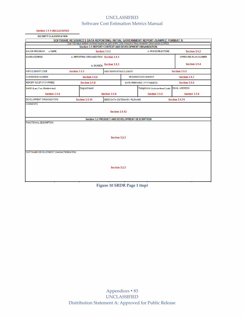
UNCLASSIFIED
Software Cost Estimation Metrics Manual
Appendices 83 UNCLASSIFIED
Distribution Statement A: Approved for Public Release
Figure 10 SRDR Page 1 (top)

UNCLASSIFIED
Software Cost Estimation Metrics Manual
Appendices 84 UNCLASSIFIED
Distribution Statement A: Approved for Public Release
Figure 10 SRDR Page 1 (bottom)

UNCLASSIFIED
Software Cost Estimation Metrics Manual
Appendices 85 UNCLASSIFIED
Distribution Statement A: Approved for Public Release
Figure 11 SRDR Page 2

UNCLASSIFIED
Software Cost Estimation Metrics Manual
Appendices 86 UNCLASSIFIED
Distribution Statement A: Approved for Public Release
9.4.1 Proposed Modifications In 2010, the modifications in Table 33 were proposed to the DCARC. Most of the
recommendations were incorporated, to some degree, in the 2011 SRDR instructions. It will take
several years before data appears with the addition data items.
The relevance of this section in this manual is for demonstrating that DCARC will evolve the
SRDR to meet future information needs. SRDR users need to be proactive with the DCARC to
express their needs for different types of data. The recommendations in Table 33were
accompanied with examples of data analysis highlighting the shortfalls in the current data
collection.
Table 33 Recommended SRDR Modifications
Current 2007 SRDR Proposed Modifications Rationale Application Types (3.7.1 – 17)
Reorganize around Operating Environments and Application Domains
Add Mission Criticality (add reliability and complexity in a single rating scale)
Revisit detailed definitions of the Application Domains
Reduce duplication Structure productivity analysis
domains, database planning guidance
Account for productivity variations
Amount of New (>25%), Modified (<25% mod) Code
Add DM, CM, IM, SU, & UNFM factors for modified code
Incorporate Galorath-like questionnaire
Add IM for reused code Definitions for code types Count at the level it will be
maintained
Improve derivation of equivalent SLOC for use in calibration and estimation
Excludes COTS; more accurate for generated code
Includes the code base for evolutionary acquisition
Deleted Code Report deleted code counts Deleting code does take effort
Software and External Interface Requirements
Add anticipated requirements volatility to 2630-1, 2
Use percentage of requirements change as volatility input (SRR baseline)
CARD realism Traceability Improve calibration and
estimation accuracy
Personnel Experience & Turnover
Add to 2630-1 Expand years of experience rating
scale to 12 years
CARD realism Traceability Improve calibration and
estimation accuracy Project- or CSCI-level data
Specify the level of data reporting Apples-to-Apples comparison Improved data analysis
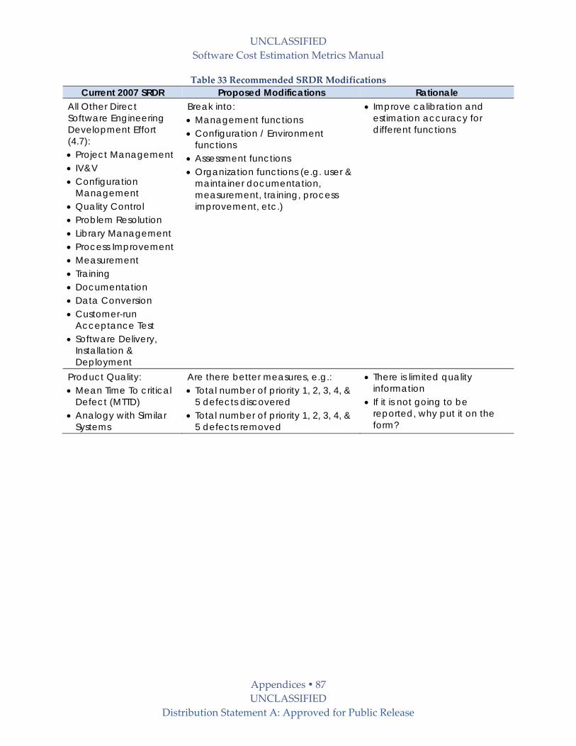
UNCLASSIFIED
Software Cost Estimation Metrics Manual
Appendices 87 UNCLASSIFIED
Distribution Statement A: Approved for Public Release
Table 33 Recommended SRDR Modifications
Current 2007 SRDR Proposed Modifications Rationale All Other Direct Software Engineering Development Effort (4.7): Project Management IV&V Configuration
Management Quality Control Problem Resolution Library Management Process Improvement Measurement Training Documentation Data Conversion Customer-run
Acceptance Test Software Delivery,
Installation & Deployment
Break into: Management functions Configuration / Environment
functions Assessment functions Organization functions (e.g. user &
maintainer documentation, measurement, training, process improvement, etc.)
Improve calibration and estimation accuracy for different functions
Product Quality: Mean Time To critical
Defect (MTTD) Analogy with Similar
Systems
Are there better measures, e.g.: Total number of priority 1, 2, 3, 4, &
5 defects discovered Total number of priority 1, 2, 3, 4, &
5 defects removed
There is limited quality information
If it is not going to be reported, why put it on the form?

UNCLASSIFIED
Software Cost Estimation Metrics Manual
Appendices 88 UNCLASSIFIED
Distribution Statement A: Approved for Public Release
9.5 MIL-STD-881C WBS Mapping to Productivity Types The Work Breakdown Structures were adapted from MIL‐STD‐881C to assist in determining the
correct Productivity Type (PT). Each System from 881C is listed with the associated one of more
Metrics Manual Operating Environments.
Within the environments, look through the Subsystems to find one that matches the component
being estimated. Each Subsystem or Sub‐Subsystem has a matching PT.
Use the PT to lookup the associated Productivity‐based CER and Model‐based CER/SER.
9.5.1 Aerial Vehicle Manned (AVM) Source: MIL‐STD‐881C Appendix‐A: Aircraft Systems
Env SubSystem Sub-Subsystem Domain PT
AVM Air Vehicle
Flight Control Subsystem VC
Auxiliary Power Subsystem VC
Hydraulic Subsystem VC
Electrical Subsystem VC
Crew Station Subsystem VC
Environmental Control Subsystem VC
Fuel Subsystem VC
Landing Gear VC
Rotor Group VC
Drive System VC
AVM Avionics
Communication / Identification
Intercoms RTE
Radio System(S) RTE
Identification Equipment (IFF) RTE
Data Links RTE
Navigation / Guidance
Radar SCP
Radio SCP
Other Essential Nav Equipment RTE
Radar Altimeter SCP
Direction Finding Set RTE
Doppler Compass SCP
AVM Avionics Mission Computer / Processing MP

UNCLASSIFIED
Software Cost Estimation Metrics Manual
Appendices 89 UNCLASSIFIED
Distribution Statement A: Approved for Public Release
Env SubSystem Sub-Subsystem Domain PT
AVM Avionics
Fire Control
Search, Target, Tracking Sensors SSP
Self-Contained Navigation RTE
Self-Contained Air Data Systems RTE
Displays, Scopes, Or Sights RTE
Bombing Computer MP
Safety Devices RTE
Data Display and Controls
Multi-Function Displays RTE
Control Display Units RTE
Display Processors MP
On-Board Mission Planning TRN
Survivability
Ferret And Search Receivers SCP
Warning Devices SCP
Electronic Countermeasures SCP
Jamming Transmitters SCP
Chaff SCP
Infra-Red Jammers SCP
Terrain-Following Radar SCP
Reconnaissance
Photographic Sensors SCP
Electronic Sensors SCP
Infrared Sensors SCP
Search Receivers SCP
Recorders SCP
Warning Devices SCP
Magazines RTE
Data Link RTE

UNCLASSIFIED
Software Cost Estimation Metrics Manual
Appendices 90 UNCLASSIFIED
Distribution Statement A: Approved for Public Release
Env SubSystem Sub-Subsystem Domain PT
AVM Avionics
Automatic Flight Control
Flight Control Computers MP
Signal Processors SCP
Data Formatting MP
Interfaces To Other Systems MP
Pressure Transducers SCP
Rate Gyros SCP
Accelerometers SCP
Motion Sensors SCP
Health Monitoring System SYS
Stores Management MP
9.5.2 Ordinance Vehicle Unmanned (OVU) Source: MIL‐STD‐881C Appendix‐C: Missile Systems
Env SubSystem Sub-Subsystem Domain PT
OVU Air Vehicle
Guidance Seeker Assembly SCP
Guidance Software RTE
Navigation Sensor Assembly SCP
Navigation Software RTE
Payload
Target Defeat Mechanism RTE
Target Detection Device SCP
Fuze SCP
Payload-specific software VP
Power and Distribution
Primary Power VC
Power Conditioning Electronics VC
Power and distribution software VC
Communications Antenna Assembly SCP
Communications software RTE

UNCLASSIFIED
Software Cost Estimation Metrics Manual
Appendices 91 UNCLASSIFIED
Distribution Statement A: Approved for Public Release
Env SubSystem Sub-Subsystem Domain PT
OVU Air Vehicle Propulsion Subsystem
Motor Engine VC
Thrust Vector Actuation VC
Attitude Control System VC
Fuel / Oxidizer Liquid Management VC
Arm / Fire Device VC
Flight Termination/Mission Termination RTE
Propulsion software VC
OVU Air Vehicle
Controls Controls software VC
Reentry System VC
Post boost System VC
On Board Test Equipment TST
On Board Training Equipment TRN
Auxiliary Equipment SYS
Air Vehicle Software MP
OVU Encasement Device
Encasement Device Software MP
OVU Command &
Launch
Surveillance, Identification, and Tracking Sensors SCP
Launch & Guidance Control RTE
Communications RTE
Launcher Equipment RTE
Auxiliary Equipment SYS
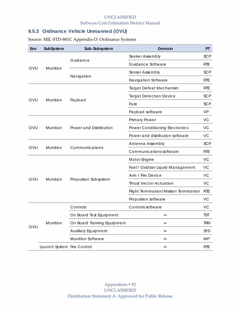
UNCLASSIFIED
Software Cost Estimation Metrics Manual
Appendices 92 UNCLASSIFIED
Distribution Statement A: Approved for Public Release
9.5.3 Ordinance Vehicle Unmanned (OVU) Source: MIL‐STD‐881C Appendix‐D: Ordinance Systems
Env SubSystem Sub-Subsystem Domain PT
OVU Munition
Guidance Seeker Assembly SCP
Guidance Software RTE
Navigation Sensor Assembly SCP
Navigation Software RTE
OVU Munition Payload
Target Defeat Mechanism RTE
Target Detection Device SCP
Fuze SCP
Payload software VP
OVU Munition Power and Distribution
Primary Power VC
Power Conditioning Electronics VC
Power and distribution software VC
OVU Munition Communications Antenna Assembly SCP
Communications software RTE
OVU Munition Propulsion Subsystem
Motor Engine VC
Fuel / Oxidizer Liquid Management VC
Arm / Fire Device VC
Thrust Vector Actuation VC
Flight Termination/Mission Termination RTE
Propulsion software VC
OVU Munition
Controls Controls software VC
On Board Test Equipment TST
On Board Training Equipment TRN
Auxiliary Equipment SYS
Munition Software MP
Launch System Fire Control RTE
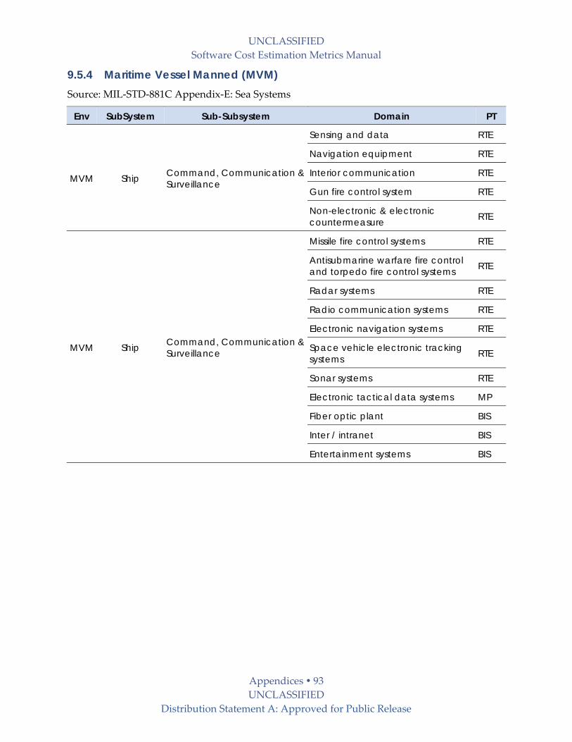
UNCLASSIFIED
Software Cost Estimation Metrics Manual
Appendices 93 UNCLASSIFIED
Distribution Statement A: Approved for Public Release
9.5.4 Maritime Vessel Manned (MVM) Source: MIL‐STD‐881C Appendix‐E: Sea Systems
Env SubSystem Sub-Subsystem Domain PT
MVM Ship Command, Communication & Surveillance
Sensing and data RTE
Navigation equipment RTE
Interior communication RTE
Gun fire control system RTE
Non-electronic & electronic countermeasure RTE
MVM Ship Command, Communication & Surveillance
Missile fire control systems RTE
Antisubmarine warfare fire control and torpedo fire control systems RTE
Radar systems RTE
Radio communication systems RTE
Electronic navigation systems RTE
Space vehicle electronic tracking systems RTE
Sonar systems RTE
Electronic tactical data systems MP
Fiber optic plant BIS
Inter / intranet BIS
Entertainment systems BIS

UNCLASSIFIED
Software Cost Estimation Metrics Manual
Appendices 94 UNCLASSIFIED
Distribution Statement A: Approved for Public Release
9.5.5 Space Vehicle Manned / Unmanned (SVM/U) and Ground Site Fixed (GSF) Source: MIL‐STD‐881C Appendix‐F: Space Systems
Env SubSystem Sub-Subsystem Domain PT
SVM/U Bus
Structures & Mechanisms (SMS) VC
Thermal Control (TCS) VC
Electrical Power (EPS) VC
Attitude Control (ACS) VC
Propulsion VC
Telemetry, Tracking, & Command (TT&C) RTE
Bus Flight Software MP
SVM/U Payload
Thermal Control RTE
Electrical Power RTE
Pointing, Command, & Control Interface VP
Payload Antenna SCP
Payload Signal Electronics SCP
Optical Assembly SCP
Sensor SCP
Payload Flight Software VP
GSF
Ground Operations
& Processing Center
Mission Management BIS
Command and Control C&C
Mission Data Processing BIS
Mission Data Analysis BIS
Collection Management BIS
Infrastructure & Framework SYS
GSF Ground
Terminal / Gateway
Ground Terminal Software Application Specific Integrated Circuit SCP
Field Programmable Gate Array SCP
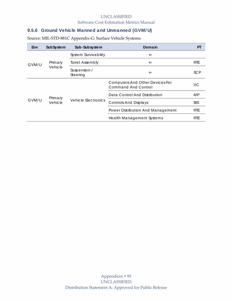
UNCLASSIFIED
Software Cost Estimation Metrics Manual
Appendices 95 UNCLASSIFIED
Distribution Statement A: Approved for Public Release
9.5.6 Ground Vehicle Manned and Unmanned (GVM/U) Source: MIL‐STD‐881C Appendix‐G: Surface Vehicle Systems
Env SubSystem Sub-Subsystem Domain PT
GVM/U Primary Vehicle
System Survivability
Turret Assembly RTE
Suspension / Steering SCP
GVM/U Primary Vehicle
Vehicle Electronics
Computers And Other Devices For Command And Control VC
Data Control And Distribution MP
Controls And Displays BIS
Power Distribution And Management RTE
Health Management Systems RTE

UNCLASSIFIED
Software Cost Estimation Metrics Manual
Appendices 96 UNCLASSIFIED
Distribution Statement A: Approved for Public Release
Env SubSystem Sub-Subsystem Domain PT
GVM/U
Primary Vehicle
Power Package / Drive Train
Controls And Instrumentation VC
Power Transmission, Final Drivers, And Power Takeoffs VC
Brakes And Steering When Integral To Power Transmission VC
Hybrid Electric Drive Systems VC
Energy Storage Systems VC
Fire Control
Radars And Other Sensors SCP
Controls And Displays RTE
Sights Or Scopes RTE
Range Finders, Gun Drives And Stabilization Systems RTE
Armament
Main Gun And Secondary Guns VP
Missile Launchers VP
Non-Lethal Weapons VP
Other Offensive Weapon Systems VP
Automatic Ammunition Handling
MP
Primary Vehicle
Navigation and Remote Piloting RTE
Communications RTE
GVU
Remote Control
System (UGV specific)
Ground Control Systems RTE
Command and Control Subsystem C&C
Remote Control System Software RTE

UNCLASSIFIED
Software Cost Estimation Metrics Manual
Appendices 97 UNCLASSIFIED
Distribution Statement A: Approved for Public Release
9.5.7 Aerial Vehicle Unmanned(AVU) & Ground Site Fixed (GSF) Source: MIL‐STD‐881C Appendix‐H: Unmanned Air Vehicle Systems
Env SubSystem Sub-Subsystem Domain PT
AVU Air Vehicle Vehicle Subsystems
Propulsion VC
Flight Control Subsystem VC
Auxiliary Power Subsystem VC
Hydraulic Subsystem VC
Electrical Subsystem VC
Environmental Control VC
Subsystem Fuel Subsystem VC
Landing Gear VC
Rotor Group VC
Drive System VC
AVU Air Vehicle Avionics
Communication / Identification RTE
Navigation / Guidance RTE
Automatic Flight Control VC
Health Monitoring System SYS
Stores Management VP
Mission Processing MP
Fire Control RTE
AVU Payload
Survivability Payload VP
Reconnaissance Payload VP
Electronic Warfare Payload VP
Armament / Weapons Delivery VP
GSF Ground / Host
Segment
Ground Control Systems C&C
Command and Control Subsystem RTE
Launch and Recovery Equipment RTE
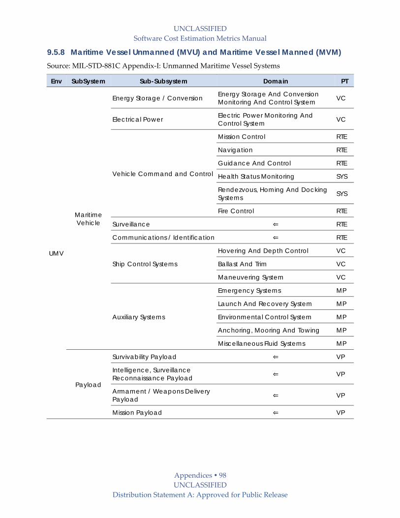
UNCLASSIFIED
Software Cost Estimation Metrics Manual
Appendices 98 UNCLASSIFIED
Distribution Statement A: Approved for Public Release
9.5.8 Maritime Vessel Unmanned (MVU) and Maritime Vessel Manned (MVM) Source: MIL‐STD‐881C Appendix‐I: Unmanned Maritime Vessel Systems
Env SubSystem Sub-Subsystem Domain PT
UMV
Maritime Vehicle
Energy Storage / Conversion Energy Storage And Conversion Monitoring And Control System VC
Electrical Power Electric Power Monitoring And Control System VC
Vehicle Command and Control
Mission Control RTE
Navigation RTE
Guidance And Control RTE
Health Status Monitoring SYS
Rendezvous, Homing And Docking Systems SYS
Fire Control RTE
Surveillance RTE
Communications / Identification RTE
Ship Control Systems
Hovering And Depth Control VC
Ballast And Trim VC
Maneuvering System VC
Auxiliary Systems
Emergency Systems MP
Launch And Recovery System MP
Environmental Control System MP
Anchoring, Mooring And Towing MP
Miscellaneous Fluid Systems MP
Payload
Survivability Payload VP
Intelligence, Surveillance Reconnaissance Payload VP
Armament / Weapons Delivery Payload VP
Mission Payload VP

UNCLASSIFIED
Software Cost Estimation Metrics Manual
Appendices 99 UNCLASSIFIED
Distribution Statement A: Approved for Public Release
Env SubSystem Sub-Subsystem Domain PT
MVM Shipboard Segment
Shipboard UM Command and Control Subsystem C&C
Shipboard Communication Subsystem RTE
Shipboard Power Subsystem VC
Launch and Recovery Equipment RTE
9.5.9 Ordinance Vehicle Unmanned (OVU) Source: MIL‐STD‐881C Appendix‐J: Launch Vehicles
Env SubSystem Sub-Subsystem Domain PT
OVU
Launch Vehicle
Stage(s)
Propulsions System VC
Reaction Control System VC
Recovery System VC
Environmental Control System RTE
Stage Peculiar Avionics RTE
Avionics
Guidance Navigation and Control RTE
Power VC
Data Acquisition and Telemetry RTE
Range Tracking & Safety (Airborne) RTE
Flight Software VC
Flight Operations
Real-time mission control
Telemetry processing RTE
Communications RTE
Data reduction and analysis BIS
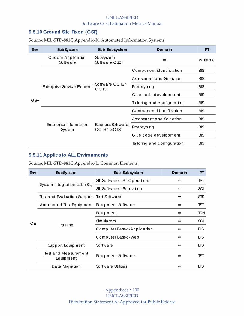
UNCLASSIFIED
Software Cost Estimation Metrics Manual
Appendices 100 UNCLASSIFIED
Distribution Statement A: Approved for Public Release
9.5.10 Ground Site Fixed (GSF) Source: MIL‐STD‐881C Appendix‐K: Automated Information Systems
Env SubSystem Sub-Subsystem Domain PT
GSF
Custom Application Software
Subsystem Software CSCI Variable
Enterprise Service Element Software COTS / GOTS
Component identification BIS
Assessment and Selection BIS
Prototyping BIS
Glue code development BIS
Tailoring and configuration BIS
Enterprise Information System
Business Software COTS / GOTS
Component identification BIS
Assessment and Selection BIS
Prototyping BIS
Glue code development BIS
Tailoring and configuration BIS
9.5.11 Applies to ALL Environments Source: MIL‐STD‐881C Appendix‐L: Common Elements
Env SubSystem Sub-Subsystem Domain PT
CE
System Integration Lab (SIL) SIL Software - SIL Operations TST
SIL Software - Simulation SCI
Test and Evaluation Support Test Software STS
Automated Test Equipment Equipment Software TST
Training
Equipment TRN
Simulators SCI
Computer Based-Application BIS
Computer Based-Web BIS
Support Equipment Software BIS
Test and Measurement Equipment Equipment Software TST
Data Migration Software Utilities BIS

UNCLASSIFIED
Software Cost Estimation Metrics Manual
Appendices 101 UNCLASSIFIED
Distribution Statement A: Approved for Public Release
9.6 Productivity (Pr) Benchmark Details
9.6.1 Normality Tests on Productivity Data Before analyzing the data for central tendencies, a check was made of the normality of each
dataset that had five (5) or more records using the Anderson‐Darling Normality Test. To reject
the hypothesis of normality, the Anderson‐Darling statistic, A2, needs to exceed the critical
value of 0.787 for the case when the mean and variance are unknown. Additionally, if the P
value is less than the level of significance, 0.05 in this case, the hypothesis of normality is
rejected.
In plain English, the dataset distribution is normally distributed if:
A2 is less than 0.787
P‐value is greater than the level of significance (0.05)
In the event of a tie, visually inspect the distribution with a normal curve overlay
For each dataset that fails the normality test, a Box‐Cox transform was used to determine the
function, Ft, required to transform the data into a more normal‐like distribution thereby
improving the validity of the measurement of the mean and median.
Table 34, Table 35and Table 36 show the results of the Anderson‐Darling test on productivity
data grouped by Operating Environments (OpEnv), Productivity Types (PT) and OpEnv‐PT
pairs. The table columns are:
Group name
N: number of records
A2:: Anderson‐Darling test statistic
P: P value
Ft: function for transforming data to a more normal‐like distribution, if required
To be included in the analysis, there were five (5) or more records in a group.
9.6.1.1 Operating Environments (all Productivity Types) Table 34 OpEnv Productivity Normality Tests
Operating Environment (OpEnv) N A2 P Ft 1 Aerial Vehicle Manned (AVM) 50 1.27 0.005 X0.5 2 Ground Site Fixed (GFS) 116 0.95 0.016 X0.5 3 Maritime Vessel Manned (MVM) 69 2.45 0.005 X0.5 4 Ordinance Vehicle Unmanned (OVU) 16 0.42 0.285 Not Required 5 Space Vehicle Unmanned (SVU) 6 0.22 0.702 Not Required

UNCLASSIFIED
Software Cost Estimation Metrics Manual
Appendices 102 UNCLASSIFIED
Distribution Statement A: Approved for Public Release
9.6.1.2 Productivity Types (all Operating Environments) Table 35 PT Productivity Normality Tests
Productivity Type (PT) N A2 P Ft 1 Intel and Information Processing (IIS) 35 0.53 0.162 Loge 2 Mission Processing (MP) 47 0.59 0.117 Loge 3 Real-Time Embedded (RTE) 53 0.17 0.927 Loge 4 Scientific Systems (SCI) 39 0.76 0.044 x1.5 5 Sensor Control and Signal Processing (SCP) 38 0.62 0.100 Not Required 6 System Software (SYS) 60 0.30 0.566 Not Required
9.6.1.3 Operating Environment – Productivity Type Sets
To be included in the analysis, there has to be five (5) or more records in the OpEnv‐PT pair.
This caused some operating environments and productivity types to drop out of consideration.
Table 36 OpEnv - PT Normality Tests
OpEnv - PT N A2 P Ft 1 AVM-MP 31 1.89 0.005 Loge 2 AVM-RTE 9 0.832 0.019 Loge 3 AVM-SCP 8 0.227 0.725 Not Required 4 GSF-IIS 23 0.44 0.274 Not Required 5 GSF-MP 6 0.23 0.661 Not Required 6 GSF-RTE 23 0.41 0.310 Not Required 7 GSF-SCI 23 0.95 0.013 X2 8 GSF-SCP 13 0.86 0.020 X2 9 GSF-SYS 28 0.30 0.571 Not Required 10 MVM-MP 8 0.44 0.200 Not Required 11 MVM-RTE 6 0.58 0.074 Loge 12 MVM-SCI 15 0.54 0.141 Not Required 13 MVM-SCP 7 0.43 0.217 Not Required 14 MVM-SYS 28 0.53 0.159 Not Required 15 OVU-RTE 11 0.27 0.593 Not Required
9.6.2 Statistical Summaries on Productivity Data The following sections show statistical summaries of the non‐transformed and, if required, the
transformed productivity data. The transformation function, Ft, is shown in the summary table
above the histogram.

UNCLASSIFIED
Software Cost Estimation Metrics Manual
Appendices 103 Unclassified: Distribution Statement A / Approved for Public Release
9.6.2.1 Operating Environments Non-Transformed Transformed with Ft
400320240160800
Median
Mean
180160140120100
1st Quartile 80.46Median 129.303rd Quartile 183.86
Maximum 389.56
120.88 171.99
102.23 151.27
75.11 112.05
A-Squared 1.27P-Value < 0.005
Mean 146.43StDev 89.92
Variance 8085.32Skewness 1.02934Kurtosis 0.66251N 50
Minimum 9.24
Anderson-Darling Normality Test
95% Confidence Interval for Mean
95% Confidence Interval for Median
95% Confidence Interval for StDev95% Confidence Intervals
Summary forAVM-Pr
20161284
Median
Mean
12.512.011.511.010.510.0
1st Quartile 8.970Median 11.3703rd Quartile 13.559
Maximum 19.737
10.502 12.586
10.111 12.299
3.062 4.568
A-Squared 0.28P-Value 0.628
Mean 11.544StDev 3.666
Variance 13.437Skewness 0.274914Kurtosis -0.067340N 50
Minimum 3.039
Anderson-Darling Normality Test
95% Confidence Interval for Mean
95% Confidence Interval for Median
95% Confidence Interval for StDev95% Confidence Intervals
Summary for AVM-SqRt(Pr)

UNCLASSIFIED
Software Cost Estimation Metrics Manual
Appendices 104 UNCLASSIFIED
Distribution Statement A: Approved for Public Release
Non-Transformed Transformed with Ft
600500400300200100
Median
Mean
260240220200180
1st Quartile 117.51Median 228.763rd Quartile 301.22
Maximum 580.72
200.57 245.22
182.26 261.01
107.53 139.40
A-Squared 0.95P-Value 0.016
Mean 222.90StDev 121.40
Variance 14736.90Skewness 0.417306Kurtosis -0.326034N 116
Minimum 26.82
Anderson-Darling Normality Test
95% Confidence Interval for Mean
95% Confidence Interval for Median
95% Confidence Interval for StDev95% Confidence Intervals
Summary for GSF-Pr
242118151296
Median
Mean
16.516.015.515.014.514.013.5
1st Quartile 10.839Median 15.1233rd Quartile 17.356
Maximum 24.098
13.522 15.096
13.500 16.156
3.791 4.914
A-Squared 0.96P-Value 0.015
Mean 14.309StDev 4.279
Variance 18.313Skewness -0.152076Kurtosis -0.747428N 116
Minimum 5.179
Anderson-Darling Normality Test
95% Confidence Interval for Mean
95% Confidence Interval for Median
95% Confidence Interval for StDev95% Confidence Intervals
Summary for GSF-SqRt(Pr)

UNCLASSIFIED
Software Cost Estimation Metrics Manual
Appendices 105 UNCLASSIFIED
Distribution Statement A: Approved for Public Release
Non-Transformed Transformed with Ft
6404803201600
Median
Mean
280260240220200180160
1st Quartile 111.73Median 193.343rd Quartile 324.33
Maximum 716.86
191.20 279.57
169.14 233.40
154.82 218.33
A-Squared 2.56P-Value < 0.005
Mean 235.38StDev 181.14
Variance 32811.65Skewness 1.30544Kurtosis 1.38414N 67
Minimum 20.24
Anderson-Darling Normality Test
95% Confidence Interval for Mean
95% Confidence Interval for Median
95% Confidence Interval for StDev95% Confidence Intervals
Summary for MVM-Pr
252015105
Median
Mean
16.015.515.014.514.013.513.0
1st Quartile 10.570Median 13.9053rd Quartile 18.009
Maximum 26.774
12.855 15.648
13.005 15.277
4.893 6.901
A-Squared 0.64P-Value 0.092
Mean 14.251StDev 5.725
Variance 32.779Skewness 0.413780Kurtosis -0.138233N 67
Minimum 4.499
Anderson-Darling Normality Test
95% Confidence Interval for Mean
95% Confidence Interval for Median
95% Confidence Interval for StDev95% Confidence Intervals
Summary for MVM-SqRt(Pr)

UNCLASSIFIED
Software Cost Estimation Metrics Manual
Appendices 106 UNCLASSIFIED
Distribution Statement A: Approved for Public Release
Non-Transformed Transformed with Ft
Not Required 300250200150100500
Median
Mean
2001751501251007550
1st Quartile 50.78Median 119.943rd Quartile 225.61
Maximum 277.35
84.38 180.62
52.74 202.87
66.71 139.76
A-Squared 0.42P-Value 0.285
Mean 132.50StDev 90.30
Variance 8154.88Skewness 0.23432Kurtosis -1.36368N 16
Minimum 9.95
Anderson-Darling Normality Test
95% Confidence Interval for Mean
95% Confidence Interval for Median
95% Confidence Interval for StDev95% Confidence Intervals
Summary for OVU-Pr

UNCLASSIFIED
Software Cost Estimation Metrics Manual
Appendices 107 UNCLASSIFIED
Distribution Statement A: Approved for Public Release
Non-Transformed Transformed with Ft
Not Required 1601208040
Median
Mean
1501251007550
1st Quartile 52.411Median 76.0203rd Quartile 125.189
Maximum 152.927
38.892 130.884
39.521 139.719
27.359 107.496
A-Squared 0.22P-Value 0.702
Mean 84.888StDev 43.829
Variance 1921.005Skewness 0.509669Kurtosis 0.074706N 6
Minimum 27.802
Anderson-Darling Normality Test
95% Confidence Interval for Mean
95% Confidence Interval for Median
95% Confidence Interval for StDev95% Confidence Intervals
Summary for SVU-Pr
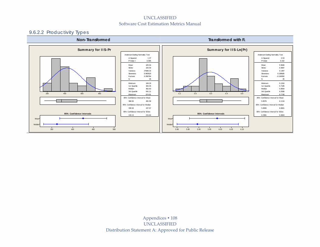
UNCLASSIFIED
Software Cost Estimation Metrics Manual
Appendices 108 UNCLASSIFIED
Distribution Statement A: Approved for Public Release
9.6.2.2 Productivity Types Non-Transformed Transformed with Ft
800600400200
Median
Mean
500450400350
1st Quartile 304.45Median 362.633rd Quartile 541.11
Maximum 874.81
368.50 481.58
330.50 437.97
133.13 215.64
A-Squared 1.37P-Value < 0.005
Mean 425.04StDev 164.59
Variance 27089.34Skewness 0.983520Kurtosis 0.356784N 35
Minimum 169.29
Anderson-Darling Normality Test
95% Confidence Interval for Mean
95% Confidence Interval for Median
95% Confidence Interval for StDev95% Confidence Intervals
Summary for IIS-Pr
6.86.46.05.65.2
Median
Mean
6.106.056.005.955.905.855.80
1st Quartile 5.7185Median 5.89343rd Quartile 6.2936
Maximum 6.7740
5.8576 6.1116
5.8006 6.0821
0.2991 0.4844
A-Squared 0.53P-Value 0.162
Mean 5.9846StDev 0.3697
Variance 0.1367Skewness 0.198585Kurtosis -0.194392N 35
Minimum 5.1316
Anderson-Darling Normality Test
95% Confidence Interval for Mean
95% Confidence Interval for Median
95% Confidence Interval for StDev95% Confidence Intervals
Summary for IIS-Ln(Pr)

UNCLASSIFIED
Software Cost Estimation Metrics Manual
Appendices 109 UNCLASSIFIED
Distribution Statement A: Approved for Public Release
Non-Transformed Transformed with Ft
6404803201600
Median
Mean
220200180160140
1st Quartile 124.37Median 159.323rd Quartile 236.43
Maximum 716.86
156.66 221.49
138.37 183.91
91.74 138.67
A-Squared 2.65P-Value < 0.005
Mean 189.07StDev 110.41
Variance 12189.41Skewness 2.6731Kurtosis 10.5868N 47
Minimum 34.44
Anderson-Darling Normality Test
95% Confidence Interval for Mean
95% Confidence Interval for Median
95% Confidence Interval for StDev95% Confidence Intervals
Summary for MP-Pr
6.45.64.84.0
Median
Mean
5.35.25.15.04.9
1st Quartile 4.8233Median 5.07093rd Quartile 5.4656
Maximum 6.5749
4.9719 5.2628
4.9299 5.2144
0.4118 0.6224
A-Squared 0.59P-Value 0.117
Mean 5.1174StDev 0.4955
Variance 0.2456Skewness 0.03841Kurtosis 2.20613N 47
Minimum 3.5392
Anderson-Darling Normality Test
95% Confidence Interval for Mean
95% Confidence Interval for Median
95% Confidence Interval for StDev95% Confidence Intervals
Summary for MP-Ln(Pr)
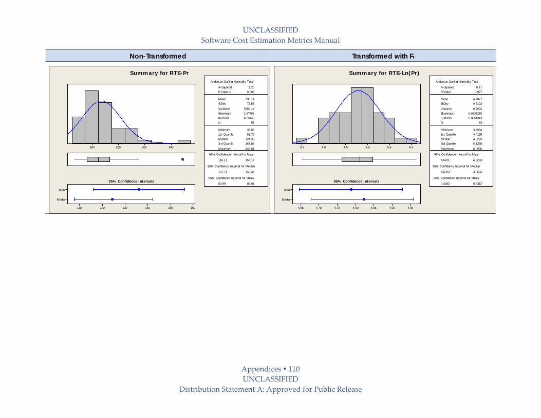
UNCLASSIFIED
Software Cost Estimation Metrics Manual
Appendices 110 UNCLASSIFIED
Distribution Statement A: Approved for Public Release
Non-Transformed Transformed with Ft
400300200100
Median
Mean
160150140130120110
1st Quartile 82.73Median 124.333rd Quartile 167.84
Maximum 443.01
116.11 156.17
107.71 142.35
60.99 89.91
A-Squared 1.26P-Value < 0.005
Mean 136.14StDev 72.66
Variance 5280.14Skewness 1.67782Kurtosis 4.85448N 53
Minimum 33.06
Anderson-Darling Normality Test
95% Confidence Interval for Mean
95% Confidence Interval for Median
95% Confidence Interval for StDev95% Confidence Intervals
Summary for RTE-Pr
6.05.55.04.54.03.5
Median
Mean
4.954.904.854.804.754.704.65
1st Quartile 4.4155Median 4.82293rd Quartile 5.1230
Maximum 6.0936
4.6471 4.9283
4.6793 4.9583
0.4282 0.6312
A-Squared 0.17P-Value 0.927
Mean 4.7877StDev 0.5102
Variance 0.2603Skewness -0.0835250Kurtosis 0.0854313N 53
Minimum 3.4984
Anderson-Darling Normality Test
95% Confidence Interval for Mean
95% Confidence Interval for Median
95% Confidence Interval for StDev95% Confidence Intervals
Summary for RTE-Ln(Pr)

UNCLASSIFIED
Software Cost Estimation Metrics Manual
Appendices 111 UNCLASSIFIED
Distribution Statement A: Approved for Public Release
Non-Transformed Transformed with Ft
4003002001000
Median
Mean
280260240220200180160
1st Quartile 106.28Median 247.683rd Quartile 313.11
Maximum 431.11
182.45 259.60
167.52 280.60
97.25 153.37
A-Squared 0.90P-Value 0.019
Mean 221.03StDev 119.00
Variance 14161.76Skewness -0.21790Kurtosis -1.15300N 39
Minimum 9.24
Anderson-Darling Normality Test
95% Confidence Interval for Mean
95% Confidence Interval for Median
95% Confidence Interval for StDev95% Confidence Intervals
Summary for SCI-Pr
80006000400020000
Median
Mean
5000450040003500300025002000
1st Quartile 1095.6Median 3898.03rd Quartile 5540.5
Maximum 8951.1
2836.0 4476.6
2170.0 4700.3
2068.1 3261.3
A-Squared 0.76P-Value 0.044
Mean 3656.3StDev 2530.5
Variance 6403504.9Skewness 0.155112Kurtosis -0.989185N 39
Minimum 28.1
Anderson-Darling Normality Test
95% Confidence Interval for Mean
95% Confidence Interval for Median
95% Confidence Interval for StDev95% Confidence Intervals
Summary for SCI-(Pr^1.5)

UNCLASSIFIED
Software Cost Estimation Metrics Manual
Appendices 112 UNCLASSIFIED
Distribution Statement A: Approved for Public Release
Non-Transformed Transformed with Ft
Not Required 80604020
Median
Mean
6055504540
1st Quartile 32.964Median 52.6083rd Quartile 66.526
Maximum 80.043
43.426 56.194
37.728 60.386
15.834 25.127
A-Squared 0.62P-Value 0.100
Mean 49.810StDev 19.422
Variance 377.224Skewness -0.17597Kurtosis -1.13890N 38
Minimum 9.951
Anderson-Darling Normality Test
95% Confidence Interval for Mean
95% Confidence Interval for Median
95% Confidence Interval for StDev95% Confidence Intervals
Summary for SCI-Pr

UNCLASSIFIED
Software Cost Estimation Metrics Manual
Appendices 113 UNCLASSIFIED
Distribution Statement A: Approved for Public Release
Non-Transformed Transformed with Ft
Not Required
40032024016080
Median
Mean
250240230220210200190
1st Quartile 171.46Median 219.153rd Quartile 274.11
Maximum 421.14
204.50 244.98
193.16 245.78
66.42 95.57
A-Squared 0.30P-Value 0.566
Mean 224.74StDev 78.35
Variance 6139.38Skewness 0.368573Kurtosis -0.131695N 60
Minimum 60.61
Anderson-Darling Normality Test
95% Confidence Interval for Mean
95% Confidence Interval for Median
95% Confidence Interval for StDev95% Confidence Intervals
Summary for SYS-Pr

UNCLASSIFIED
Software Cost Estimation Metrics Manual
Appendices 114 UNCLASSIFIED
Distribution Statement A: Approved for Public Release
9.6.2.3 Operating Environment - Productivity Type Sets Non-Transformed Transformed with Ft
400300200100
Median
Mean
200180160140120
1st Quartile 121.76Median 140.933rd Quartile 188.41
Maximum 389.56
141.18 205.82
125.59 171.30
70.42 117.79
A-Squared 1.90P-Value < 0.005
Mean 173.50StDev 88.12
Variance 7764.96Skewness 1.20981Kurtosis 0.75188N 31
Minimum 34.44
Anderson-Darling Normality Test
95% Confidence Interval for Mean
95% Confidence Interval for Median
95% Confidence Interval for StDev95% Confidence Intervals
Summary for AVM_MP-Pr
6.05.55.04.54.03.5
Median
Mean
5.25.15.04.94.8
1st Quartile 4.8021Median 4.94833rd Quartile 5.2386
Maximum 5.9650
4.8567 5.2226
4.8330 5.1434
0.3986 0.6667
A-Squared 0.72P-Value 0.055
Mean 5.0396StDev 0.4988
Variance 0.2488Skewness -0.32485Kurtosis 1.75426N 31
Minimum 3.5392
Anderson-Darling Normality Test
95% Confidence Interval for Mean
95% Confidence Interval for Median
95% Confidence Interval for StDev95% Confidence Intervals
Summary for AVM_MP-ln(Pr)

UNCLASSIFIED
Software Cost Estimation Metrics Manual
Appendices 115 UNCLASSIFIED
Distribution Statement A: Approved for Public Release
Non-Transformed Transformed with Ft
25020015010050
Median
Mean
250200150100
1st Quartile 81.31Median 89.043rd Quartile 237.23
Maximum 242.86
80.05 199.90
80.13 239.66
52.66 149.35
A-Squared 0.83P-Value 0.019
Mean 139.98StDev 77.96
Variance 6077.32Skewness 0.57445Kurtosis -1.82660N 9
Minimum 56.96
Anderson-Darling Normality Test
95% Confidence Interval for Mean
95% Confidence Interval for Median
95% Confidence Interval for StDev95% Confidence Intervals
Summary for AVM_RTE-Pr
5.24.84.44.0
Median
Mean
5.505.255.004.754.50
1st Quartile 4.3979Median 4.48903rd Quartile 5.4689
Maximum 5.4925
4.3720 5.2322
4.3834 5.4791
0.3779 1.0719
A-Squared 0.60P-Value 0.079
Mean 4.8021StDev 0.5595
Variance 0.3131Skewness 0.26890Kurtosis -1.74694N 9
Minimum 4.0424
Anderson-Darling Normality Test
95% Confidence Interval for Mean
95% Confidence Interval for Median
95% Confidence Interval for StDev95% Confidence Intervals
Summary for AVM_RTE-ln(Pr)

UNCLASSIFIED
Software Cost Estimation Metrics Manual
Appendices 116 UNCLASSIFIED
Distribution Statement A: Approved for Public Release
Non-Transformed Transformed with Ft
Not Required 70605040
Median
Mean
706560555045
1st Quartile 46.146Median 57.8353rd Quartile 67.806
Maximum 70.440
45.344 66.813
44.133 68.559
8.489 26.133
A-Squared 0.23P-Value 0.725
Mean 56.078StDev 12.840
Variance 164.866Skewness -0.679094Kurtosis -0.347898N 8
Minimum 33.322
Anderson-Darling Normality Test
95% Confidence Interval for Mean
95% Confidence Interval for Median
95% Confidence Interval for StDev95% Confidence Intervals
Summary for AVM_SCP-Pr
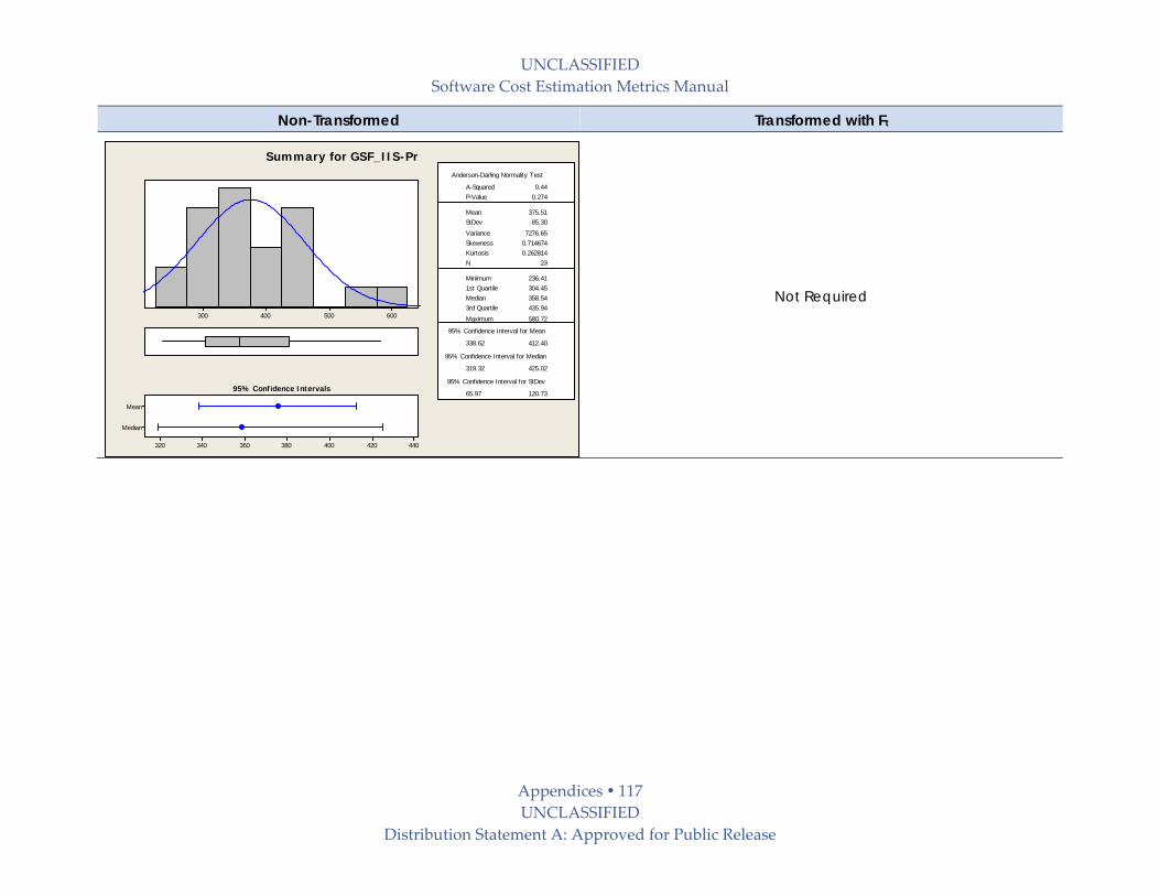
UNCLASSIFIED
Software Cost Estimation Metrics Manual
Appendices 117 UNCLASSIFIED
Distribution Statement A: Approved for Public Release
Non-Transformed Transformed with Ft
Not Required 600500400300
Median
Mean
440420400380360340320
1st Quartile 304.45Median 358.543rd Quartile 435.94
Maximum 580.72
338.62 412.40
319.32 425.02
65.97 120.73
A-Squared 0.44P-Value 0.274
Mean 375.51StDev 85.30
Variance 7276.65Skewness 0.714674Kurtosis 0.262814N 23
Minimum 236.41
Anderson-Darling Normality Test
95% Confidence Interval for Mean
95% Confidence Interval for Median
95% Confidence Interval for StDev95% Confidence Intervals
Summary for GSF_IIS-Pr

UNCLASSIFIED
Software Cost Estimation Metrics Manual
Appendices 118 UNCLASSIFIED
Distribution Statement A: Approved for Public Release
Non-Transformed Transformed with Ft
Not Required 24020016012080
Median
Mean
220200180160140120100
1st Quartile 125.49Median 158.303rd Quartile 199.44
Maximum 243.16
107.59 215.79
105.47 222.34
32.18 126.44
A-Squared 0.23P-Value 0.661
Mean 161.69StDev 51.55
Variance 2657.58Skewness 0.28077Kurtosis 1.21448N 6
Minimum 87.27
Anderson-Darling Normality Test
95% Confidence Interval for Mean
95% Confidence Interval for Median
95% Confidence Interval for StDev95% Confidence Intervals
Summary for GSF_MP-Pr

UNCLASSIFIED
Software Cost Estimation Metrics Manual
Appendices 119 UNCLASSIFIED
Distribution Statement A: Approved for Public Release
Non-Transformed Transformed with Ft
Not Required 25020015010050
Median
Mean
150140130120110
1st Quartile 99.29Median 130.333rd Quartile 148.53
Maximum 239.18
109.25 148.33
106.88 142.16
34.95 63.96
A-Squared 0.41P-Value 0.310
Mean 128.79StDev 45.19
Variance 2042.14Skewness 0.681898Kurtosis 0.726621N 23
Minimum 51.22
Anderson-Darling Normality Test
95% Confidence Interval for Mean
95% Confidence Interval for Median
95% Confidence Interval for StDev95% Confidence Intervals
Summary for GSF_RTE-Pr

UNCLASSIFIED
Software Cost Estimation Metrics Manual
Appendices 120 UNCLASSIFIED
Distribution Statement A: Approved for Public Release
Non-Transformed Transformed with Ft
400300200100
Median
Mean
320300280260240220200
1st Quartile 200.99Median 274.213rd Quartile 313.11
Maximum 410.23
211.35 295.85
246.89 307.19
75.56 138.28
A-Squared 0.95P-Value 0.013
Mean 253.60StDev 97.70
Variance 9545.01Skewness -0.676131Kurtosis -0.289559N 23
Minimum 60.70
Anderson-Darling Normality Test
95% Confidence Interval for Mean
95% Confidence Interval for Median
95% Confidence Interval for StDev95% Confidence Intervals
Summary for GSF_SCI-Pr
16000012000080000400000
Median
Mean
1000009000080000700006000050000
1st Quartile 40398Median 751893rd Quartile 98039
Maximum 168289
54086 92802
60953 94388
34622 63359
A-Squared 0.48P-Value 0.210
Mean 73444StDev 44766
Variance 2003968683Skewness 0.152910Kurtosis -0.156978N 23
Minimum 3685
Anderson-Darling Normality Test
95% Confidence Interval for Mean
95% Confidence Interval for Median
95% Confidence Interval for StDev95% Confidence Intervals
Summary for GSF_SCI-(Pr^2)

UNCLASSIFIED
Software Cost Estimation Metrics Manual
Appendices 121 UNCLASSIFIED
Distribution Statement A: Approved for Public Release
Non-Transformed Transformed with Ft
807060504030
Median
Mean
6560555045
1st Quartile 43.952Median 60.3473rd Quartile 66.740
Maximum 80.043
45.991 66.057
48.128 66.582
11.906 27.407
A-Squared 0.86P-Value 0.020
Mean 56.024StDev 16.603
Variance 275.653Skewness -0.857414Kurtosis -0.221174N 13
Minimum 26.819
Anderson-Darling Normality Test
95% Confidence Interval for Mean
95% Confidence Interval for Median
95% Confidence Interval for StDev95% Confidence Intervals
Summary for GSF_SCP-Pr
600050004000300020001000
Median
Mean
45004000350030002500
1st Quartile 2059.7Median 3641.73rd Quartile 4454.4
Maximum 6406.9
2379.0 4407.4
2426.8 4433.3
1203.5 2770.5
A-Squared 0.53P-Value 0.140
Mean 3393.2StDev 1678.3
Variance 2816765.6Skewness -0.333019Kurtosis -0.159418N 13
Minimum 719.3
Anderson-Darling Normality Test
95% Confidence Interval for Mean
95% Confidence Interval for Median
95% Confidence Interval for StDev95% Confidence Intervals
Summary for GSF_SCP(Pr^2)

UNCLASSIFIED
Software Cost Estimation Metrics Manual
Appendices 122 UNCLASSIFIED
Distribution Statement A: Approved for Public Release
Non-Transformed Transformed with Ft
Not Required 400350300250200150100
Median
Mean
270260250240230220210
1st Quartile 199.19Median 245.293rd Quartile 274.11
Maximum 421.14
215.54 264.87
213.01 265.11
50.29 86.57
A-Squared 0.30P-Value 0.571
Mean 240.20StDev 63.60
Variance 4045.48Skewness 0.56326Kurtosis 1.35086N 28
Minimum 115.23
Anderson-Darling Normality Test
95% Confidence Interval for Mean
95% Confidence Interval for Median
95% Confidence Interval for StDev95% Confidence Intervals
Summary for GSF_SYS-Pr

UNCLASSIFIED
Software Cost Estimation Metrics Manual
Appendices 123 UNCLASSIFIED
Distribution Statement A: Approved for Public Release
Non-Transformed Transformed with Ft
Not Required 240220200180160140120
Median
Mean
240220200180160140120
1st Quartile 127.32Median 202.043rd Quartile 236.43
Maximum 242.48
140.68 237.10
125.86 238.04
33.59 114.79
A-Squared 0.44P-Value 0.200
Mean 188.89StDev 52.13
Variance 2717.31Skewness -0.35267Kurtosis -2.10327N 7
Minimum 121.86
Anderson-Darling Normality Test
95% Confidence Interval for Mean
95% Confidence Interval for Median
95% Confidence Interval for StDev95% Confidence Intervals
Summary for MVM_MP-Pr

UNCLASSIFIED
Software Cost Estimation Metrics Manual
Appendices 124 UNCLASSIFIED
Distribution Statement A: Approved for Public Release
Non-Transformed Transformed with Ft
4003002001000
Median
Mean
4003002001000
1st Quartile 61.90Median 110.073rd Quartile 247.29
Maximum 443.01
1.39 315.20
46.79 349.81
93.33 366.70
A-Squared 0.58P-Value 0.074
Mean 158.30StDev 149.51
Variance 22354.48Skewness 1.78797Kurtosis 3.44193N 6
Minimum 33.06
Anderson-Darling Normality Test
95% Confidence Interval for Mean
95% Confidence Interval for Median
95% Confidence Interval for StDev95% Confidence Intervals
Summary for MVM_RTE-Pr
6.05.55.04.54.03.5
Median
Mean
6.05.55.04.54.0
1st Quartile 4.0770Median 4.65173rd Quartile 5.4266
Maximum 6.0936
3.7865 5.6700
3.7739 5.7760
0.5601 2.2009
A-Squared 0.18P-Value 0.853
Mean 4.7282StDev 0.8974
Variance 0.8053Skewness 0.269630Kurtosis 0.103773N 6
Minimum 3.4984
Anderson-Darling Normality Test
95% Confidence Interval for Mean
95% Confidence Interval for Median
95% Confidence Interval for StDev95% Confidence Intervals
Summary for MVM_RTE-Ln(Pr)

UNCLASSIFIED
Software Cost Estimation Metrics Manual
Appendices 125 UNCLASSIFIED
Distribution Statement A: Approved for Public Release
Non-Transformed Transformed with Ft
Not Required 400300200100
Median
Mean
30025020015010050
1st Quartile 54.51Median 169.463rd Quartile 326.65
Maximum 431.11
112.75 257.65
56.10 296.19
95.79 206.34
A-Squared 0.54P-Value 0.141
Mean 185.20StDev 130.83
Variance 17117.26Skewness 0.51734Kurtosis -1.05039N 15
Minimum 36.11
Anderson-Darling Normality Test
95% Confidence Interval for Mean
95% Confidence Interval for Median
95% Confidence Interval for StDev95% Confidence Intervals
Summary for MVM_SCI-Pr

UNCLASSIFIED
Software Cost Estimation Metrics Manual
Appendices 126 UNCLASSIFIED
Distribution Statement A: Approved for Public Release
Non-Transformed Transformed with Ft
Not Required 80706050403020
Median
Mean
6050403020
1st Quartile 23.505Median 33.0713rd Quartile 45.978
Maximum 77.186
21.079 56.713
22.635 54.300
12.414 42.422
A-Squared 0.43P-Value 0.217
Mean 38.896StDev 19.265
Variance 371.132Skewness 1.48446Kurtosis 2.51764N 7
Minimum 20.243
Anderson-Darling Normality Test
95% Confidence Interval for Mean
95% Confidence Interval for Median
95% Confidence Interval for StDev95% Confidence Intervals
Summary for MVM_SCP-Pr

UNCLASSIFIED
Software Cost Estimation Metrics Manual
Appendices 127 UNCLASSIFIED
Distribution Statement A: Approved for Public Release
Non-Transformed Transformed with Ft
Not Required 400350300250200150100
Median
Mean
280260240220200
1st Quartile 177.76Median 202.153rd Quartile 303.39
Maximum 393.13
195.26 273.45
188.54 278.50
65.71 124.03
A-Squared 0.53P-Value 0.159
Mean 234.35StDev 85.89
Variance 7376.37Skewness 0.515429Kurtosis -0.673920N 21
Minimum 103.63
Anderson-Darling Normality Test
95% Confidence Interval for Mean
95% Confidence Interval for Median
95% Confidence Interval for StDev95% Confidence Intervals
Summary for MVM_SYS-Pr
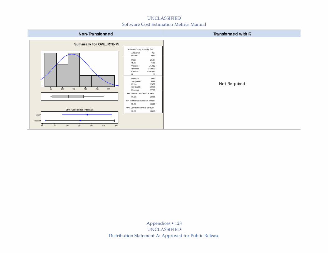
UNCLASSIFIED
Software Cost Estimation Metrics Manual
Appendices 128 UNCLASSIFIED
Distribution Statement A: Approved for Public Release
Non-Transformed Transformed with Ft
Not Required 30025020015010050
Median
Mean
2001751501251007550
1st Quartile 55.68Median 126.723rd Quartile 192.35
Maximum 277.35
90.09 192.05
55.51 196.20
53.02 133.17
A-Squared 0.27P-Value 0.593
Mean 141.07StDev 75.88
Variance 5758.12Skewness 0.429912Kurtosis -0.693482N 11
Minimum 49.82
Anderson-Darling Normality Test
95% Confidence Interval for Mean
95% Confidence Interval for Median
95% Confidence Interval for StDev95% Confidence Intervals
Summary for OVU_RTE-Pr
UNCLASSIFIED
Software Cost Estimation Metrics Manual
Appendices 129 UNCLASSIFIED
Distribution Statement A: Approved for Public Release
9.7 References [Abts 2004] Abts C, ʺExtending the COCOMO II Software Cost Model to
Estimate Effort and Schedule for Software Systems Using
Commercial‐off‐the‐Shelf (COTS) Software Components: The
COCOTS Model,ʺ PhD Dissertation, Department of Industrial and
Systems Engineering, University of Southern California, May 2004
[Anderson 2010] Anderson D, Kanban, Blue Hole Press, 2010
[Banker‐Kemerer 1989] Banker, R. and Kemerer, C., “Scale Economies in New Software
Development.” IEEE Transactions on Software Engineering, Vol
15, No 10, October 1989.
[Beck 2000] Beck, K., Extreme Programming Explained, Addison‐Wesley,
2000.
[Boehm 1981] Boehm B., Software Engineering Economics. Englewood Cliffs, NJ,
Prentice‐Hall, 1981
[Boehm et al. 2000] Boehm B., Abts C., Brown W., Chulani S., Clark B., Horowitz E.,
Madachy R., Reifer D., Steece B., Software Cost Estimation with
COCOMO II, Prentice‐Hall, 2000
[Boehm et al. 2000b] Boehm B, Abts C, Chulani S, “Software Development Cost
Estimation Approaches – A Survey”, USC‐CSE‐00‐505, 2000
[Boehm et al. 2004] Boehm B, Bhuta J, Garlan D, Gradman E, Huang L, Lam A,
Madachy R, Medvidovic N, Meyer K, Meyers S, Perez G,
Reinholtz KL, Roshandel R, Rouquette N, “Using Empirical
Testbeds to Accelerate Technology Maturity and Transition: The
SCRover Experience”, Proceedings of the 2004 International
Symposium on Empirical Software Engineering, IEEE Computer
Society, 2004
[Boehm‐Lee 2005] Boehm B and Lee K, ʺEmpirical Results from an Experiment on
Value‐Based Review (VBR) Processes,ʺ Proceedings, ISESE 2005,
September 2005
[Boehm 2009] Boehm B, “Applying the Incremental Commitment Model to
Brownfield System Development,” Proceedings, CSER 2009.
[Boehm‐Lane] Boehm, B.W. and Lane, J.A, “Using the Incremental Commitment
Model to Integrate System Acquisition, Systems Engineering and
Software Engineering”, Tech Report 2007‐715, University of
Southern California, 2007.

UNCLASSIFIED
Software Cost Estimation Metrics Manual
Appendices 130 UNCLASSIFIED
Distribution Statement A: Approved for Public Release
[Boehm‐Lane 2010] Boehm B and Lane J, “ʺDoD Systems Engineering and
Management Implications for Evolutionary Acquisition of Major
Defense Systems,ʺ Proceedings, CSER 2010.
[Bisignani‐Reed 1988] Bisignani M., and Reed T, “Software Security Costing Issues”,
COCOMO Usersʹ Group Meeting.. Los Angeles: USC Center for
Software Engineering, 1988.
[Booch 2009] Personal communication from Grady Booch, IBM, 2009
[Broy 2010] Broy M, “Seamless Method‐ and Model‐based Software and
Systems Engineering,” The Future of Software Engineering,
Springer, 2010.
[Cohn 2005] Cohn M, Agile Estimating and Planning, Prentice Hall, 2005
[Colbert‐Boehm 2008] Colbert E and Boehm B, ʺCost Estimation for Secure Software &
Systems,ʺ ISPA / SCEA 2008 Joint International Conference, June
2008
[CSSE 2000] Guidelines for Model‐Based (System) Architecting and Software
Engineering (MBASE)”, available at
http://sunset.usc.edu/classes_cs577b, 2000.
[DCARC 2005] Defense Cost and Resource Center, “The DoD Software Resource
Data Report – An Update,” Proceedings of the Practical Software
Measurement (PSM) Users’ Group Conference, 19 July 2005
[Galorath 2005] Galorath Inc., SEER‐SEM User Manual, 2005
[Brooks 1995] Brooks, F., The Mythical Man‐Month, Addison‐Wesley, 1995.
[DSRC 2005] Defense Cost and Resource Center, “The DoD Software Resource
Data Report – An Update,” Proceedings of the Practical Software
Measurement (PSM) Users’ Group Conference, 19 July 2005.
[Elssamadisy‐ Elssamadisy A. and Schalliol G., Recognizing and Responding
Schalliol 2002] to ‘Bad Smells’ in Extreme Programming, Proceedings, ICSE 2002,
pp. 617‐622
[Galorath‐Evans 2006] Galorath D, Evans M, Software Sizing, Estimation, and Risk
Management, Auerbach Publications, 2006
[Garmus‐Heron 2000] Garmus, David and David Herron. Function Point Analysis:
Measurement Practices for Successful Software Projects. Boston,
Mass.: Addison Wesley, 2000
[Gill‐Iansiti 1994] Gill G., and Iansiti M., “Microsoft Corporation: Office Business
Unit,” Harvard Business School Case Study 691‐033, 1994.

UNCLASSIFIED
Software Cost Estimation Metrics Manual
Appendices 131 UNCLASSIFIED
Distribution Statement A: Approved for Public Release
[Goethert et al 1992] Goethert W, Bailey E, and Busby M, “Software Effort and
Schedule Measurement: A Framework for Counting Staff‐Hours
and Reporting Schedule Information.” Software Engineering
Institute, Carnegie Mellon University, ESC‐TR‐92‐021, 1992.
[Hopkins‐Jenkins 2008] Hopkins R, and Jenkins K, Eating the IT Elephant: Moving from
Greenfield Development to Brownfield, IBM Press.
[IFPUG 1994] Function Point Counting Practices: Manual Release 4.0,
International Function Point Users’ Group, Blendonview Office
Park, 5008‐28 Pine Creek Drive, Westerville, OH 43081‐4899.
[IFPUG 2009] International Function Points User’s Group, http://www.ifpug.org
[ISO 12207] ISO/IEC 12207, International Standard on Information Technology
Software Lifecycle Processes, International Organization for
Standardization (ISO), 1995.
[ISO 1999] ISO JTC 1/SC 27, Evaluation Criteria for IT Security, in Part 1:
Introduction and general model, International Organization for
Standardization (ISO), 1999.
[Jensen 1983] Jensen R, “An Improved Macrolevel Software Development
Resource Estimation Model”, Proceedings of 5th ISPA Conference,
1983
[Koolmanojwong‐ Koolmanojwong S and Boehm B, ʺThe Incremental
Boehm 2010] Commitment Model Process Patterns for Rapid‐Fielding
Projects,ʺProceedings, ICSP 2010, Paderborn, Germany.
[Kruchten 1998] Kruchten, P., The Rational Unified Process, Addison‐Wesley, 1998.
[Lane 2009] Lane J., ʺCost Model Extensions to Support Systems Engineering
Cost Estimation for Complex Systems and Systems of Systems,ʺ
7th Annual Conference on Systems Engineering Research 2009
(CSER 2009)
[Lane‐Boehm 2007] Lane J., and Boehm B., ʺModern Tools to Support DoD Software
Intensive System of Systems Cost Estimation ‐ A DACS State‐of‐
the‐Art Report,ʺ August 2007.
[Lewis et al. 2008] Lewis G et al., “SMART: Analyzing the Reuse Potential of Legacy
Components on a Service‐Oriented Architecture Environment,”
CMU/SEI‐2008‐TN‐008.
[Li et al. 2009] Li Q, Li M, Yang Y, Wang Q, Tan T, Boehm B, Hu C, Bridge the
Gap between Software Test Process and Business Value: A Case
Study. Proceedings, ICSP 2009, pp. 212‐223.

UNCLASSIFIED
Software Cost Estimation Metrics Manual
Appendices 132 UNCLASSIFIED
Distribution Statement A: Approved for Public Release
[Lum et al. 2001] Lum K, Powell J, Hihn J, “Validation of Spacecraft Software Cost
Estimation Models for Flight and Ground Systems”, JPL Report,
2001
[Madachy 1997] Madachy R, Heuristic Risk Assessment Using Cost Factors”, IEEE
Software, May 1997
[Madachy‐Boehm 2006] Madachy R, Boehm B, “A Model of Options and Costs for Reliable
Autonomy (MOCA) Final Report”, reported submitted to NASA
for USRA contract #4481, 2006
[Madachy‐Boehm 2008] Madachy R, Boehm B, “Comparative Analysis of COCOMO II,
SEER‐SEM and True‐S Software Cost Models”, USC‐CSSE‐2008‐
816, 2008
[NCCA‐AFCAA 2008] Naval Center for Cost Analysis and Air Force Cost Analysis
Agency, Software Development Cost Estimation Handbook
Volume 1 (Draft), Software Technology Support Center,
September 2008
[Nguyen 2010] Nguyen V. ʺImproved Size and Effort Estimation Models for
Software Maintenance,ʺ PhD Dissertation, Department of
Computer Science, University of Southern California, December
2010,
http://csse.usc.edu/csse/TECHRPTS/by_author.html#Nguyen
[Park 1988] Park R, “The Central Equations of the PRICE Software Cost
Model”, COCOMO User’s Group Meeting, 1988
[Park 1992] Park R, “Software Size Measurement: A Framework for Counting
Source Statements,” Software Engineering Institue, Carnegie
Mellon University, ESC‐TR‐92‐020, 1992
[Putnam 1978] Putnam, L.H., “Example of an Early Sizing, Cost and Schedule
Estimate for an Application Software System,” Computer
Software and Applications Conference (COMPSAC), 1978
[Putnam‐Myers 1992] Putnam, L.H., and W. Myers. Measures for Excellence Reliable
Software on Time, Within Budget. Prentice‐Hall, Inc. Englewood
Cliffs, NJ, 1992
[Putnam‐Myers 2003] Putnam, L.H., and W. Myers. Five Core Metrics. Dorset House
Publishing. New York, NY, 2003
[PRICE 2005] PRICE Systems, TRUE S User Manual, 2005
[QSM 2003] Quantitative Software Management, SLIM Estimate for Windows
Userʹs Guide, 2003

UNCLASSIFIED
Software Cost Estimation Metrics Manual
Appendices 133 UNCLASSIFIED
Distribution Statement A: Approved for Public Release
[Reifer et al. 1999] Reifer D, Boehm B, Chulani S, “The Rosetta Stone ‐ Making
COCOMO 81 Estimates Work with COCOMO II”, Crosstalk, 1999
[Reifer 2008] Reifer, D., “Twelve Myths of Maintenance,” Reifer Consultants,
Inc., 2008.
[Reifer 2002] Reifer, D., “Let the Numbers Do the Talking,” CrossTalk, Vol. 15,
No. 3, March 2002.
[Reifer 2002] Reifer D., Security: A Rating Concept for COCOMO II. 2002.
Reifer Consultants, Inc.
[Royce 1998] Royce, W., Software Project Management: A Unified Framework,
Addison‐Wesley, 1998.
[Schwaber‐ Schwaber, K. and Beedle, M., Scrum: Agile Software
Beedle 2002] Development, Prentice‐Hall, 2002.
[Selby 1988] Selby R, “Empirically Analyzing Software Reuse in a Production
Environment”, In Software Reuse: Emerging Technology, W.
Tracz (Ed.), IEEE Computer Society Press, 1988
[Stutzke 2005] Stutzke, Richard D, Estimating Software‐Intensive Systems, Upper
Saddle River, N.J.: Addison Wesley, 2005
[Tan et al. 2009] Tan,T, Li Q, Boehm B, Yang Y, He M, and Moazeni R,
ʺProductivity Trends in Incremental and Iterative Software
Development,ʺ Proceedings, ACM‐IEEE ESEM 2009.
[Tan 2012] Tan, T, “Domain‐Based Effort Distribution Model for Software
Cost Estimation,” PhD Dissertation, Computer Science
Department, University of Southern California, June 2012.
[USC 2006] University of Southern California Center for Software
Engineering, Model Comparison Report, Report to NASA AMES,
Draft Version, July 2006
[USD (AT&L) 2008] Systems Engineering Guide for System of Systems, Version 1.0,
OUSD(AT&L), June 2008.
[Valerdi 2011] Valerdi R, Systems Engineering Cost Estimation with COSYSMO,
Wiley, 2011.
[Yang et al. 2005] Yang Y, Bhuta J, Boehm B, and Port D, ʺValue‐Based Processes for
COTS‐Based Applications,ʺ IEEE Software, Volume 22, Issue 4,
July‐August 2005, pp. 54‐62
Related Documents