Martin-Luther-Universität Halle-Wittenberg Title Review of Numerical Methods for Multiphase Flow M. Sommerfeld Mechanische Verfahrenstechnik Zentrum für Ingenieurwissenschaften Martin-Luther-Universität Halle-Wittenberg 06099 Halle (Saale), Germany www-mvt.iw.uni-halle.de

Welcome message from author
This document is posted to help you gain knowledge. Please leave a comment to let me know what you think about it! Share it to your friends and learn new things together.
Transcript
Martin-Luther-Universität Halle-Wittenberg
Title
Review of Numerical Methods for Multiphase Flow
M. Sommerfeld
Mechanische Verfahrenstechnik Zentrum für Ingenieurwissenschaften Martin-Luther-Universität Halle-Wittenberg 06099 Halle (Saale), Germany www-mvt.iw.uni-halle.de
Martin-Luther-Universität Halle-Wittenberg
Content of the Lecture
Classification of multiphase flows Classification of numerical methods for multiphase flows. Particle-resolved direct numerical simulations Interface tracking method for bubbly flows Lattice-Boltzmann method (particle resolved) Direct numerical simulations with point-particles Approaches with turbulence modelling (point-particles) Euler/Euler (two fluid) approach
Euler/Lagrange approach
Summary/Conclusions
Martin-Luther-Universität Halle-Wittenberg
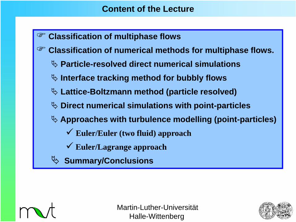
Classification of Multiphase Flows 1 Multiphase flows may be encountered in various forms:
Transient two-phase flows
Separated two-phase flows
Dispersed two-phase flows
The two-fluid concept is suitable, but requires methods for handling the interface (e.g.Tracking, VOF,.............)
Martin-Luther-Universität Halle-Wittenberg
Classification of Multiphase Flows 2
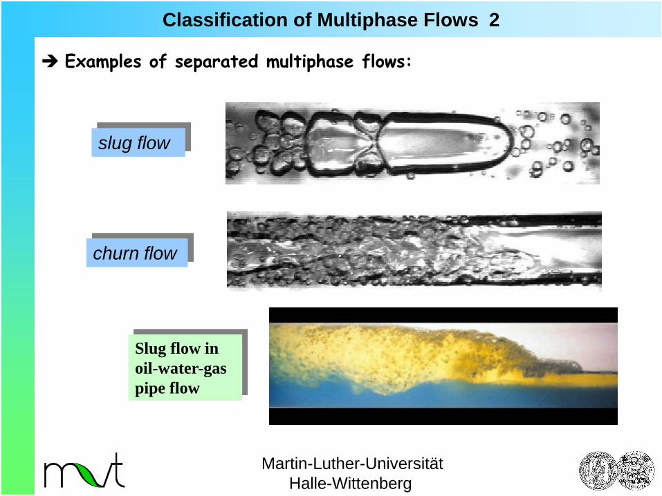
Examples of separated multiphase flows:
slug flow
churn flow
Slug flow in oil-water-gas pipe flow
Martin-Luther-Universität Halle-Wittenberg
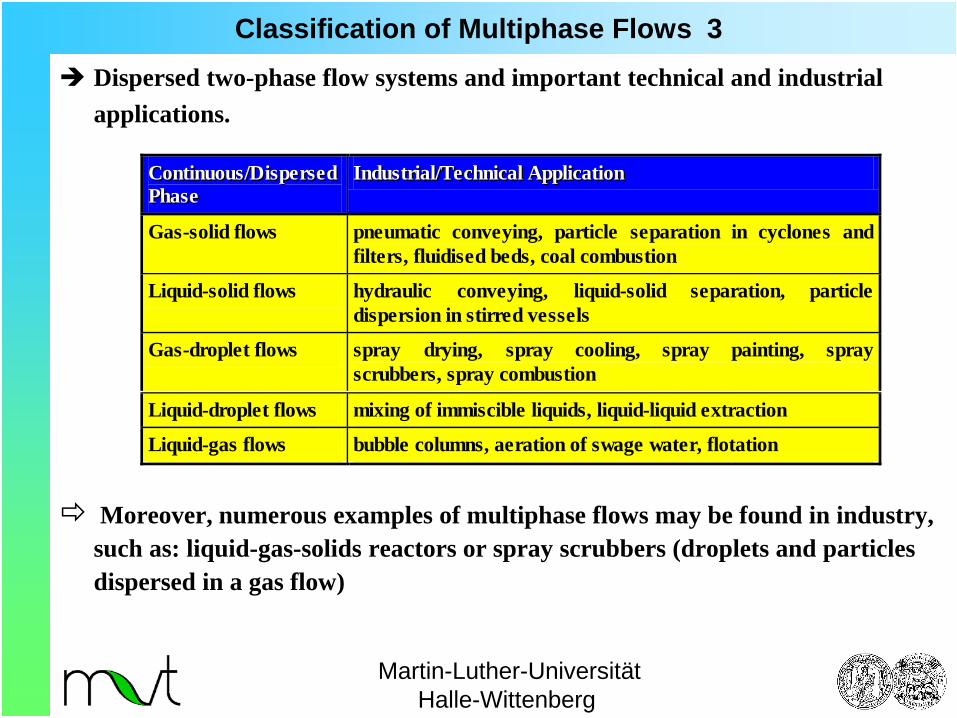
Classification of Multiphase Flows 3 Dispersed two-phase flow systems and important technical and industrial
applications.
Moreover, numerous examples of multiphase flows may be found in industry, such as: liquid-gas-solids reactors or spray scrubbers (droplets and particles dispersed in a gas flow)
CCoonnttiinnuuoouuss //DDiissppeerrsseedd PPhhaassee
IInndduussttrriiaall//TTeecchhnniiccaall AApppplliiccaattiioonn
Gas-solid flows pneumatic conveying, particle separation in cyclones and filters, fluidised beds, coal combustion
Liquid-solid flows hydraulic conveying, liquid-solid separation, particle dispersion in stirred vessels
Gas-droplet flows spray drying, spray cooling, spray painting, spray scrubbers, spray combustion
Liquid-droplet flows mixing of immiscible liquids, liquid-liquid extraction
Liquid-gas flows bubble columns, aeration of swage water, flotation
Martin-Luther-Universität Halle-Wittenberg
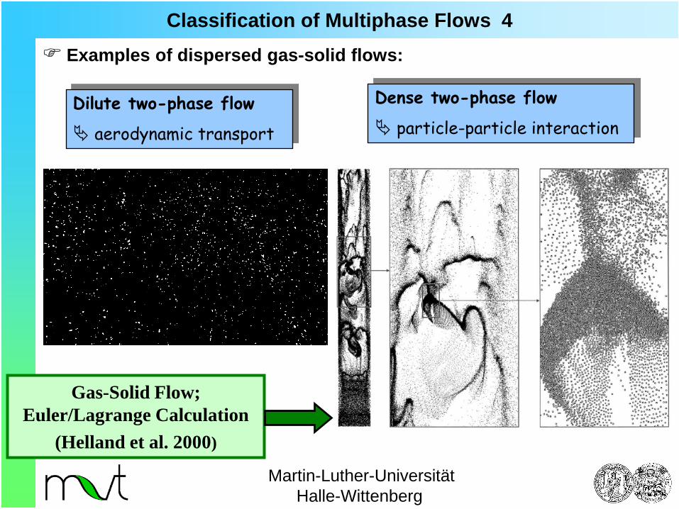
Examples of dispersed gas-solid flows:
Dilute two-phase flow
aerodynamic transport
Dense two-phase flow
particle-particle interaction
Classification of Multiphase Flows 2 Classification of Multiphase Flows 4
Gas-Solid Flow; Euler/Lagrange Calculation
(Helland et al. 2000)
Martin-Luther-Universität Halle-Wittenberg
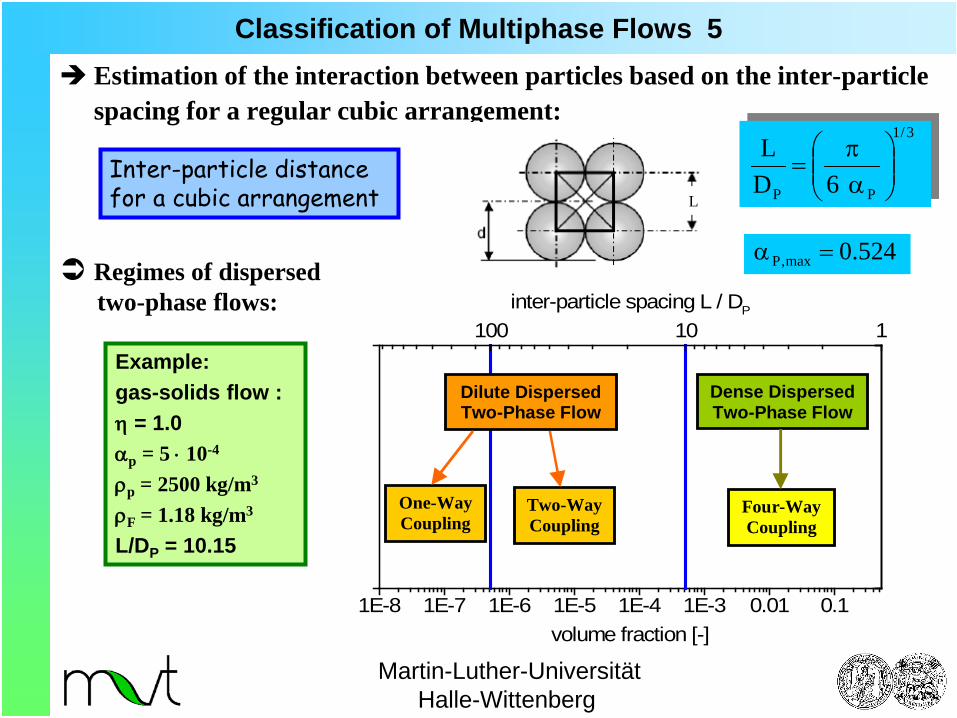
Estimation of the interaction between particles based on the inter-particle spacing for a regular cubic arrangement:
Regimes of dispersed two-phase flows:
3/1
PP 6DL
απ
=
1E-8 1E-7 1E-6 1E-5 1E-4 1E-3 0.01 0.1
volume fraction [-]
100 10 1inter-particle spacing L / DP
Dilute DispersedTwo-Phase Flow
Dense DispersedTwo-Phase Flow
Two-WayCoupling
One-WayCoupling
Four-WayCoupling
Example: gas-solids flow : η = 1.0 αp = 5 ⋅ 10-4 ρp = 2500 kg/m3
ρF = 1.18 kg/m3
L/DP = 10.15
Classification of Multiphase Flows 5 Classification of Multiphase Flows 5
L
Inter-particle distance for a cubic arrangement
524.0max,P =α
Martin-Luther-Universität Halle-Wittenberg
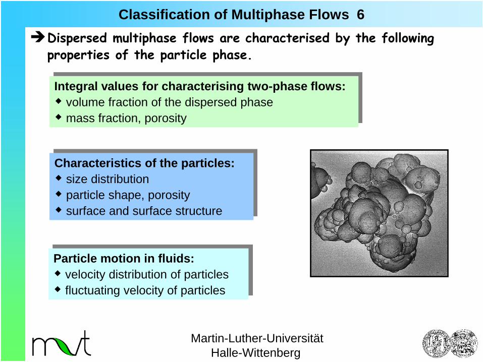
Classification of Multiphase Flows 6 Dispersed multiphase flows are characterised by the following
properties of the particle phase.
Characteristics of the particles: size distribution particle shape, porosity surface and surface structure
Particle motion in fluids: velocity distribution of particles fluctuating velocity of particles
Integral values for characterising two-phase flows: volume fraction of the dispersed phase mass fraction, porosity

Martin-Luther-Universität Halle-Wittenberg
Classification of Multiphase Flows 7 Volume fraction of the particle phase and porosity:
Effective density of both phases (or bulk density):
Mixture density:
Number concentration (particles per unit volume):
Mass loading of particles (generally only for gas-solid flows):
V
VNi
Pii
P
∑=α
PPPbP c ρα==ρ ( ) FP
bF 1 ρα−=ρ
( ) PPFPbP
bFm 1 ρα+ρα−=ρ+ρ=ρ
VNn P
P =
( ) FFP
PPP
F
P
U1U
mm
ρα−ρα
==η
P1 α−=ε
Martin-Luther-Universität Halle-Wittenberg
Numerical Methods Multiphase Flow 1
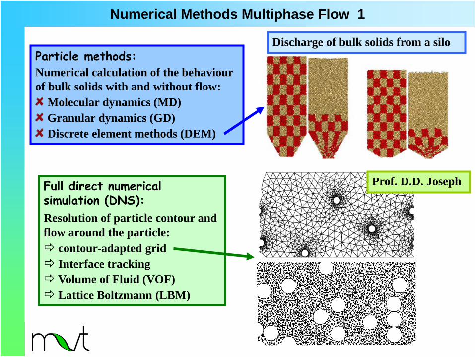
Full direct numerical simulation (DNS): Resolution of particle contour and flow around the particle: contour-adapted grid Interface tracking Volume of Fluid (VOF) Lattice Boltzmann (LBM)
Discharge of bulk solids from a silo
Prof. D.D. Joseph
Particle methods: Numerical calculation of the behaviour of bulk solids with and without flow:
Molecular dynamics (MD) Granular dynamics (GD) Discrete element methods (DEM)
Martin-Luther-Universität Halle-Wittenberg
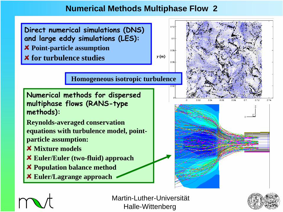
Numerical Methods Multiphase Flow 2
Direct numerical simulations (DNS) and large eddy simulations (LES):
Point-particle assumption for turbulence studies
Numerical methods for dispersed multiphase flows (RANS-type methods): Reynolds-averaged conservation equations with turbulence model, point-particle assumption:
Mixture models Euler/Euler (two-fluid) approach Population balance method Euler/Lagrange approach
Homogeneous isotropic turbulence
Martin-Luther-Universität Halle-Wittenberg
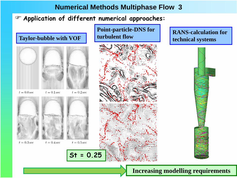
Numerical Methods Multiphase Flow 3 Application of different numerical approaches:
St = 0.25
Taylor-bubble with VOF Point-particle-DNS for turbulent flow
RANS-calculation for technical systems
Increasing modelling requirements
Martin-Luther-Universität Halle-Wittenberg
Particle-Resolved Simulations 3
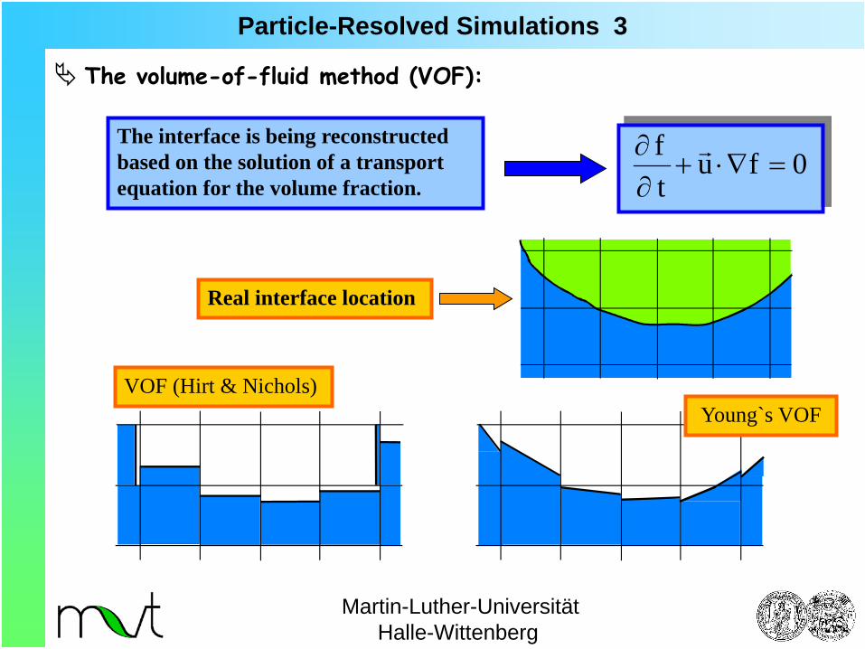
The volume-of-fluid method (VOF):
Real interface location
VOF (Hirt & Nichols)
0futf
=∇⋅+∂∂ The interface is being reconstructed
based on the solution of a transport equation for the volume fraction.
Young`s VOF
Martin-Luther-Universität Halle-Wittenberg
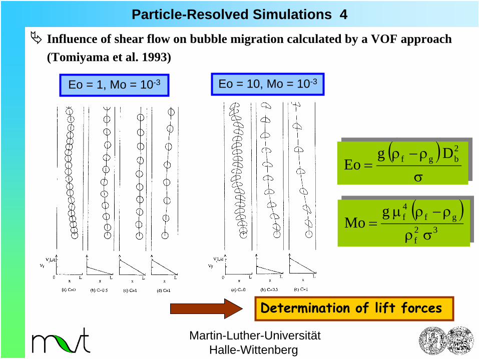
Particle-Resolved Simulations 4 Influence of shear flow on bubble migration calculated by a VOF approach
(Tomiyama et al. 1993)
Eo = 1, Mo = 10-3 Eo = 10, Mo = 10-3
( )σ
ρ−ρ=
2bgf Dg
Eo
( )32
f
gf4fg
Moσρ
ρ−ρµ=
Determination of lift forces

Martin-Luther-Universität Halle-Wittenberg
Particle-Resolved Simulations 5 Flow around nearly spherical and
large non-spherical bubbles simulated by VOF (Bothe et al. 2007)
( )σ
ρ−ρ=
2hgf
h
DgEo
( )( ) ( )( )
≤<⋅
=hh
hhBA Eo4:fürEof
4Eo:fürEof,Re121.0htan288.0minC
( ) 474.0Eo0204.0Eo0159.0Eo00105.0Eof h2h
3hh +−−=
Tomiyama correlation

Martin-Luther-Universität Halle-Wittenberg
Particle-Resolved Simulations 6 Interface resolved direct numerical simulations allow a detailed analysis of the atomisation process
Numerical grid: 128 × 128 × 896 Mesh size: 2.36 µm
Numerical grid: 256 × 256 × 2048 Mesh size: 1.17 µm
BERLEMONT 2008
Level Set/Ghost Fluid Method
Martin-Luther-Universität Halle-Wittenberg
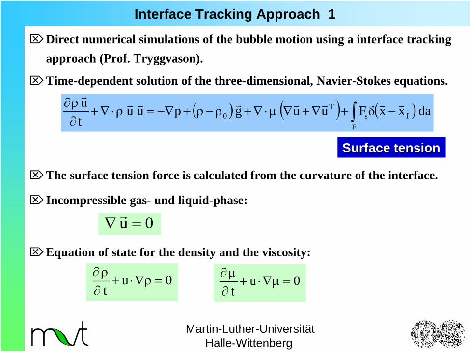
Interface Tracking Approach 1
Direct numerical simulations of the bubble motion using a interface tracking approach (Prof. Tryggvason).
Time-dependent solution of the three-dimensional, Navier-Stokes equations.
The surface tension force is calculated from the curvature of the interface.
Incompressible gas- und liquid-phase:
Equation of state for the density and the viscosity:
( ) ( ) ( )∫ −δ+∇+∇µ⋅∇+ρ−ρ+−∇=ρ⋅∇+∂ρ∂
Ffs
T0 daxxFuugpuu
tu
0ut
=ρ∇⋅+∂
ρ∂0u
t=µ∇⋅+
∂µ∂
0u =∇
Surface tension
Martin-Luther-Universität Halle-Wittenberg
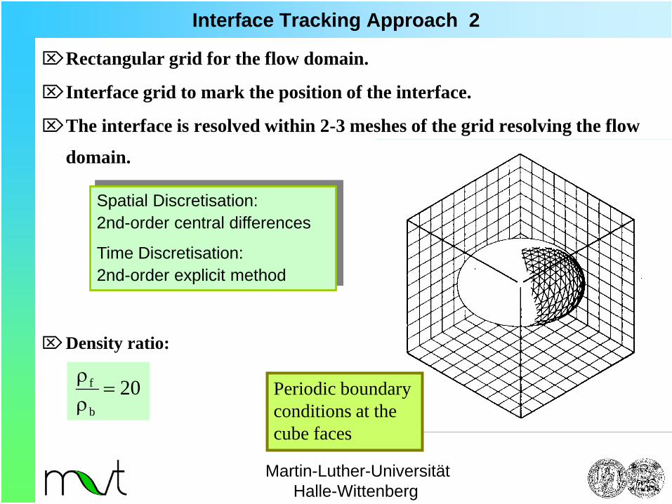
Interface Tracking Approach 2
Rectangular grid for the flow domain.
Interface grid to mark the position of the interface.
The interface is resolved within 2-3 meshes of the grid resolving the flow
domain.
Density ratio:
Spatial Discretisation: 2nd-order central differences
Time Discretisation: 2nd-order explicit method
20b
f =ρρ
Periodic boundary conditions at the cube faces
Martin-Luther-Universität Halle-Wittenberg
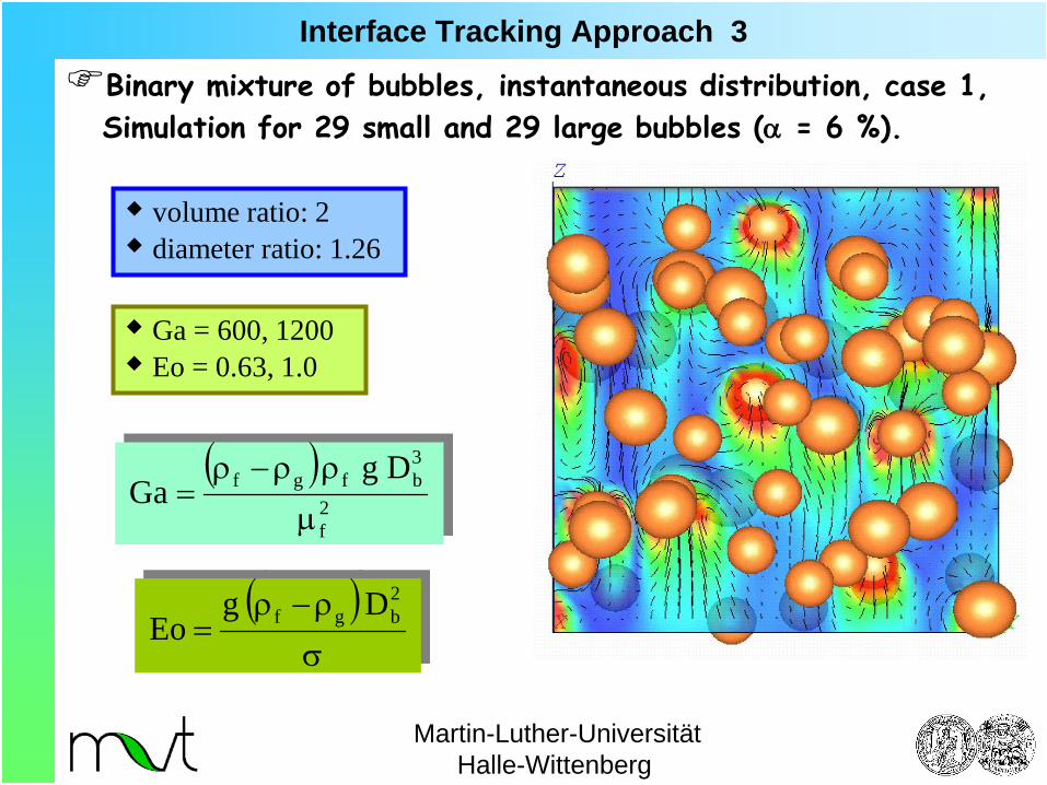
Interface Tracking Approach 3
Binary mixture of bubbles, instantaneous distribution, case 1, Simulation for 29 small and 29 large bubbles (α = 6 %).
Ga = 600, 1200 Eo = 0.63, 1.0
( )2f
3bfgf Dg
Gaµ
ρρ−ρ=
( )σ
ρ−ρ=
2bgf Dg
Eo
volume ratio: 2 diameter ratio: 1.26
Martin-Luther-Universität Halle-Wittenberg
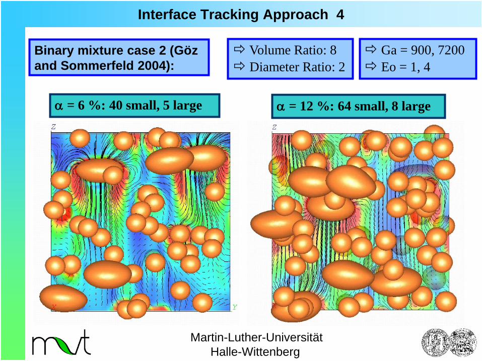
Interface Tracking Approach 4 Binary mixture case 2 (Göz and Sommerfeld 2004):
Volume Ratio: 8 Diameter Ratio: 2
Ga = 900, 7200 Eo = 1, 4
α = 6 %: 40 small, 5 large α = 12 %: 64 small, 8 large
Martin-Luther-Universität Halle-Wittenberg
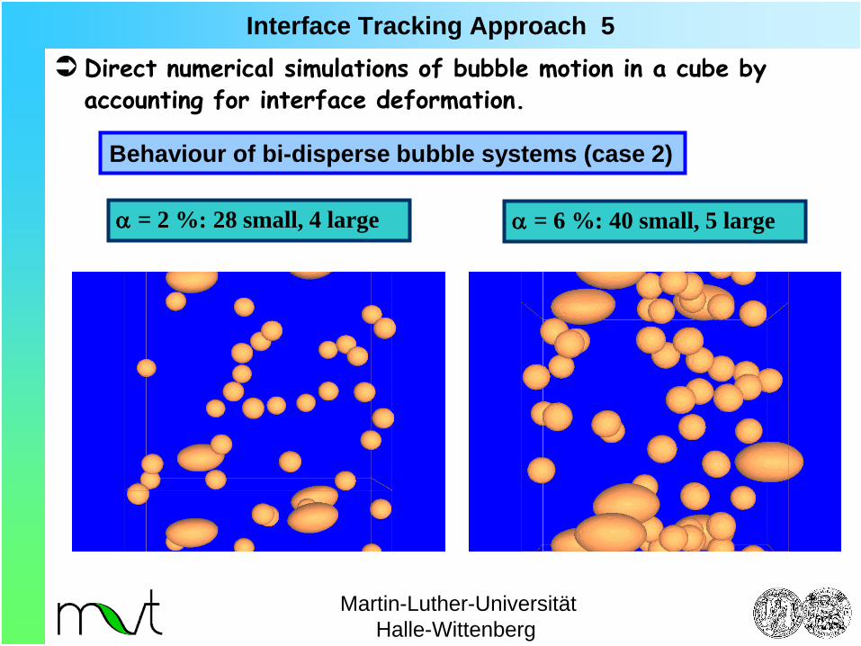
Interface Tracking Approach 5 Direct numerical simulations of bubble motion in a cube by
accounting for interface deformation.
Behaviour of bi-disperse bubble systems (case 2)
α = 2 %: 28 small, 4 large α = 6 %: 40 small, 5 large
Martin-Luther-Universität Halle-Wittenberg
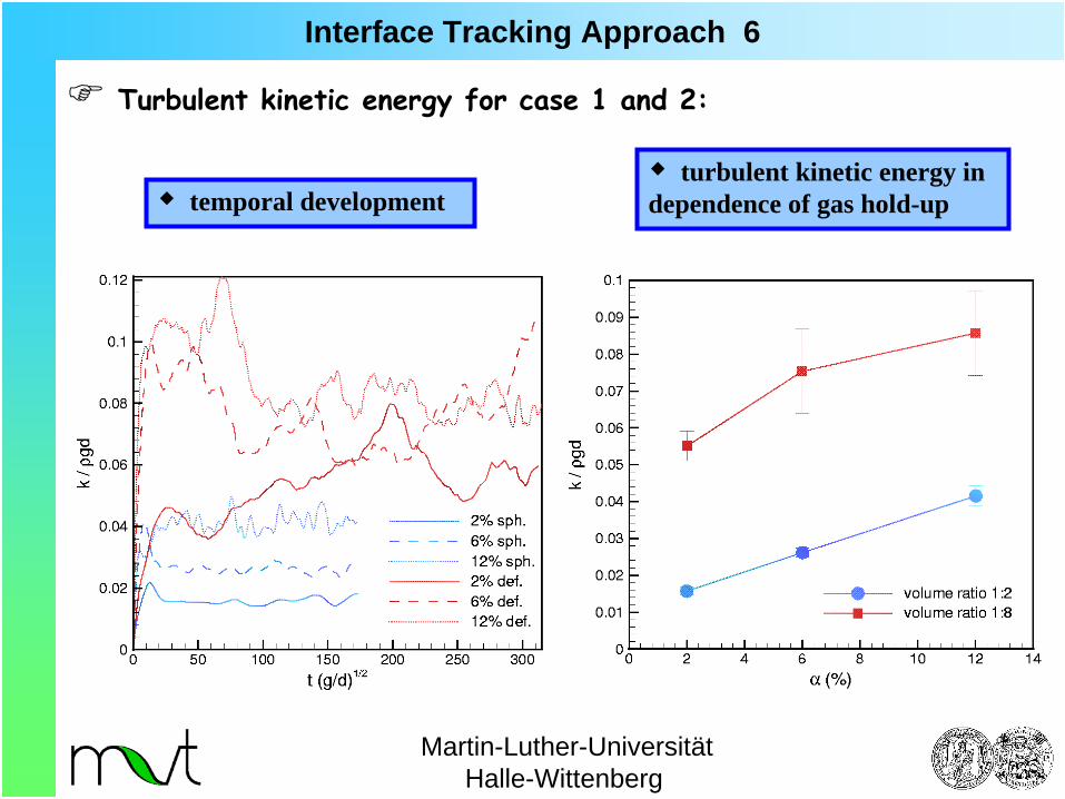
Interface Tracking Approach 6
Turbulent kinetic energy for case 1 and 2:
temporal development turbulent kinetic energy in dependence of gas hold-up
Martin-Luther-Universität Halle-Wittenberg
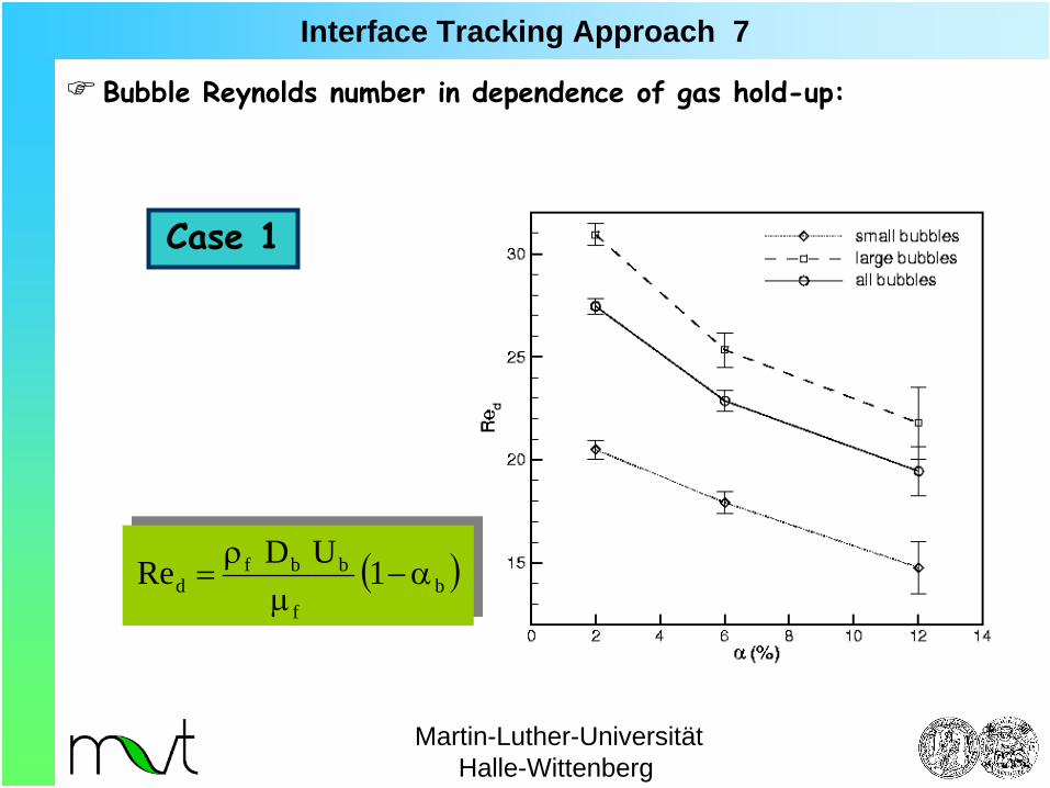
Interface Tracking Approach 7
Bubble Reynolds number in dependence of gas hold-up:
( )bf
bbfd 1UDRe α−
µρ
=
Case 1
Martin-Luther-Universität Halle-Wittenberg
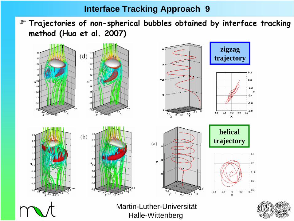
Interface Tracking Approach 9 Trajectories of non-spherical bubbles obtained by interface tracking
method (Hua et al. 2007)
zigzag trajectory
helical trajectory
Martin-Luther-Universität Halle-Wittenberg
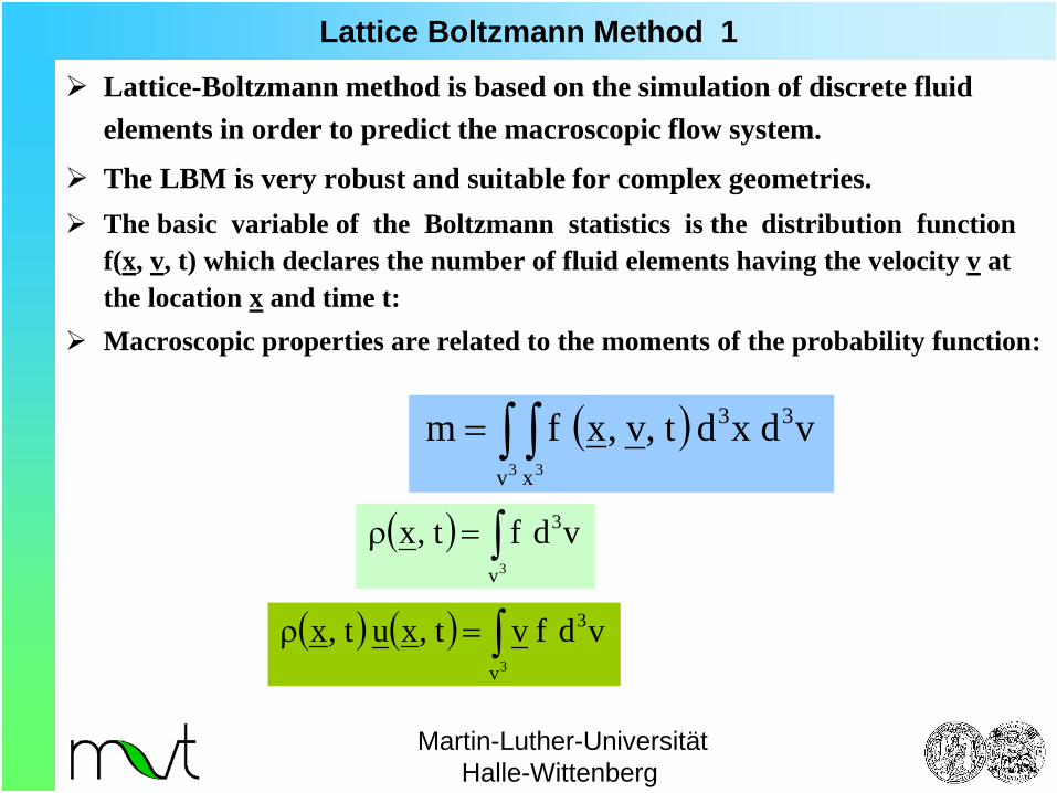
Lattice Boltzmann Method 1
Lattice-Boltzmann method is based on the simulation of discrete fluid elements in order to predict the macroscopic flow system.
The LBM is very robust and suitable for complex geometries. The basic variable of the Boltzmann statistics is the distribution function
f(x, v, t) which declares the number of fluid elements having the velocity v at the location x and time t:
Macroscopic properties are related to the moments of the probability function:
( ) ∫=ρ3v
3vdft,x
( ) ( ) ∫=ρ3v
3vdfvt,xut,x
( ) vdxdt,v,xfm3 3v x
33∫ ∫=
Martin-Luther-Universität Halle-Wittenberg
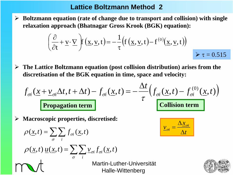
Lattice Boltzmann Method 2 Boltzmann equation (rate of change due to transport and collision) with single
relaxation approach (Bhatnagar Gross Krook (BGK) equation):
The Lattice Boltzmann equation (post collision distribution) arises from the
discretisation of the BGK equation in time, space and velocity:
Macroscopic properties, discretised:
( )),(),(),(),( )0( txftxfttxftttvxf iiiii σσσσσ τ−
∆−=−∆+∆+
∑∑=σ
σρi
i txftx ),(),(
∑∑=σ
σσρi
ii txfvtxutx ),(),(),(
Collision term
txv i
i ∆∆
= σσ
( ) ( ) ( )( )( )t,v,xft,v,xf1t,v,xfvt
0−τ
−=
∇⋅+
∂∂
Propagation term
τ = 0.515

Martin-Luther-Universität Halle-Wittenberg
Lattice Boltzmann Method 3
Discrete velocity vectors of the D3Q19 model:
Velocity vectors in the different directions:
0
2
22
2
2
2
2
22
2
1
1
1
1
1
Three-dimensional
Spatial discretisation by regular grid (voxels)
19 discrete velocity directions
Sequential solution: Propagation step Collision step
===σ±±±±±±==σ±±±
==σ
σ
121i,2,c)1,1,2(,c)1,0,1(,c)0,1,1(61i,1c)1,0,0(,c)0,1,0(,c)0,0,1(
1i,0),0,0,0(
iv
txc
∆∆
=
Lattice constant txv i
i ∆∆
= σσ

Martin-Luther-Universität Halle-Wittenberg
Lattice Boltzmann Method 4 Discrete equilibrium distribution function (Maxwellian distribution for Kn << 1):
Pressure (equation of state):
From a series expansion around the equilibrium distribution (Chapman-Enskog-Expansion) the dependence of the viscosity on the relaxation parameter (e.g. τ = 0.515 follows:
( )t2c61 2 ∆−τ=ν
−
⋅+
⋅+ω= σσ
σσ 2
2
4
2i
2i)0(
i c2)t,x(u3
c2))t,x(uv(9
c)t,x(uv31)t,x(f
==
==
==
=
121,2,361
61,1,181
1,0,31
i
i
i
σ
σ
σ
ωσ
( ) 2sc)t,x(t,xp ⋅ρ=
3ccs =
Martin-Luther-Universität Halle-Wittenberg
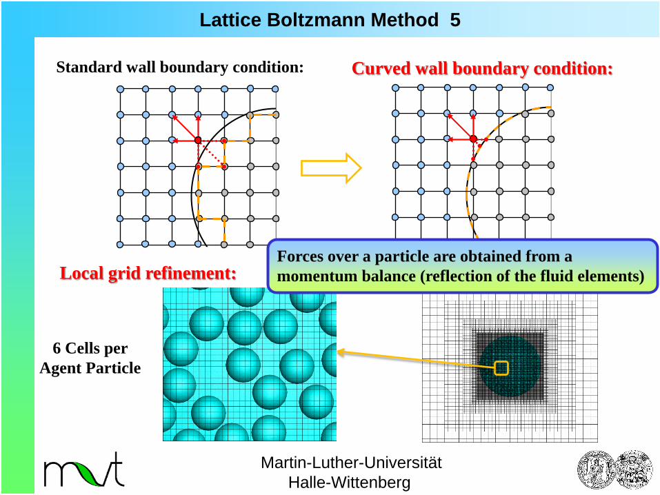
Lattice Boltzmann Method 5
Standard wall boundary condition: Curved wall boundary condition:
Local grid refinement:
6 Cells per Agent Particle
Forces over a particle are obtained from a momentum balance (reflection of the fluid elements)
Martin-Luther-Universität Halle-Wittenberg
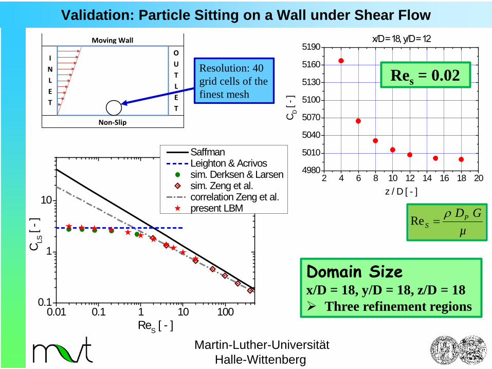
Validation: Particle Sitting on a Wall under Shear Flow
O U T L E T
Moving Wall
Non-Slip
I N L E T
2 4 6 8 10 12 14 16 18 204980
5010
5040
5070
5100
5130
5160
5190
x/D = 18, y/D = 12
C D [ -
]
z / D [ - ]
Res = 0.02
Domain Size x/D = 18, y/D = 18, z/D = 18 Three refinement regions
µGDP
Sρ
=Re
0.01 0.1 1 10 1000.1
1
10
C LS [
- ]
ReS [ - ]
Saffman Leighton & Acrivos sim. Derksen & Larsen sim. Zeng et al. correlation Zeng et al. present LBM
Resolution: 40 grid cells of the finest mesh
Martin-Luther-Universität Halle-Wittenberg
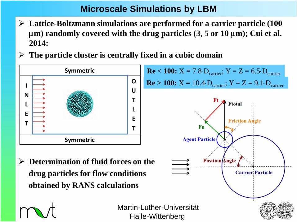
Microscale Simulations by LBM Lattice-Boltzmann simulations are performed for a carrier particle (100
µm) randomly covered with the drug particles (3, 5 or 10 µm); Cui et al. 2014:
The particle cluster is centrally fixed in a cubic domain
Determination of fluid forces on the drug particles for flow conditions obtained by RANS calculations
O U T L E T
Symmetric
Symmetric
I N L E T
Re < 100: X = 7.8⋅Dcarrier; Y = Z = 6.5⋅Dcarrier Re > 100: X = 10.4⋅Dcarrier; Y = Z = 9.1⋅Dcarrier
Martin-Luther-Universität Halle-Wittenberg
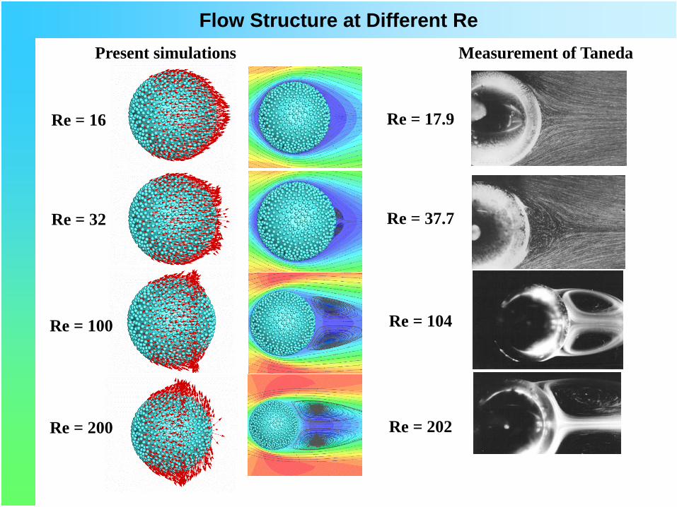
Flow Structure at Different Re
Re = 16
Re = 32
Re = 100
Re = 200
Re = 17.9
Re = 37.7
Re = 104
Re = 202
Measurement of Taneda Present simulations
Martin-Luther-Universität Halle-Wittenberg
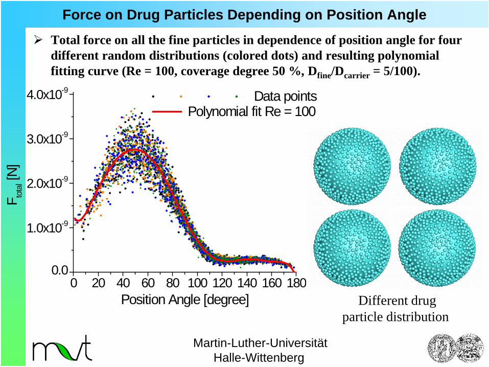
Force on Drug Particles Depending on Position Angle Total force on all the fine particles in dependence of position angle for four
different random distributions (colored dots) and resulting polynomial fitting curve (Re = 100, coverage degree 50 %, Dfine/Dcarrier = 5/100).
Data points Polynomial fit Re = 100
0 20 40 60 80 100 120 140 160 1800.0
1.0x10⁻⁹
2.0x10⁻⁹
3.0x10⁻⁹
4.0x10⁻⁹
F tota
l [N]
Position Angle [degree] Different drug particle distribution
Martin-Luther-Universität Halle-Wittenberg
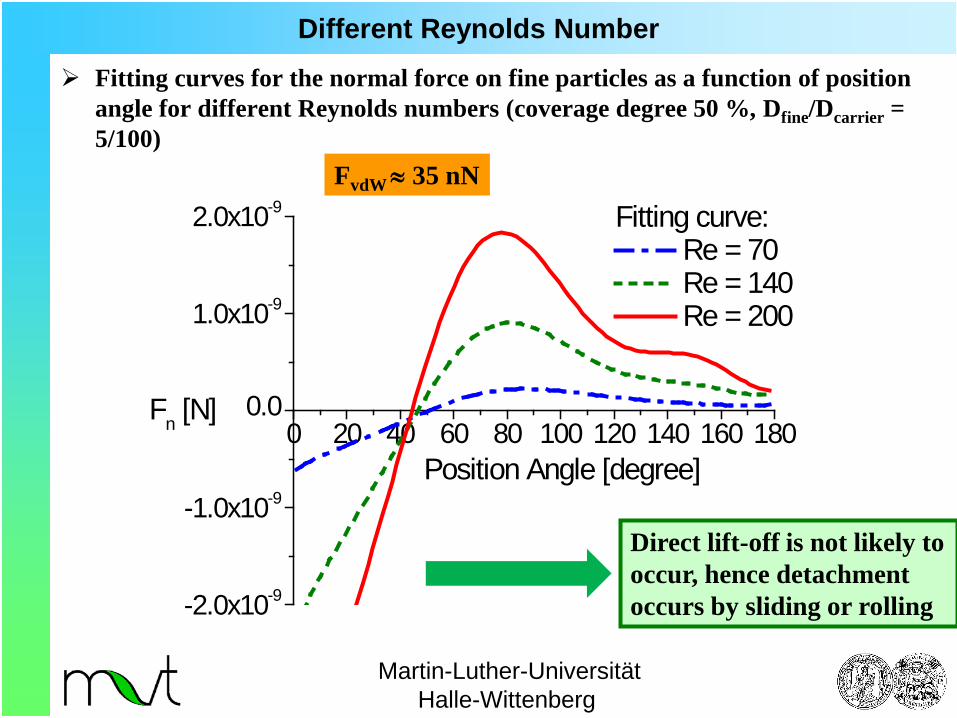
Different Reynolds Number Fitting curves for the normal force on fine particles as a function of position
angle for different Reynolds numbers (coverage degree 50 %, Dfine/Dcarrier = 5/100)
Fitting curve: Re = 70 Re = 140 Re = 200
0 20 40 60 80 100 120 140 160 180
-2.0x10⁻⁹
-1.0x10⁻⁹
0.0
1.0x10⁻⁹
2.0x10⁻⁹
Fn [N]
Position Angle [degree]
FvdW ≈ 35 nN
Direct lift-off is not likely to occur, hence detachment occurs by sliding or rolling
Martin-Luther-Universität Halle-Wittenberg
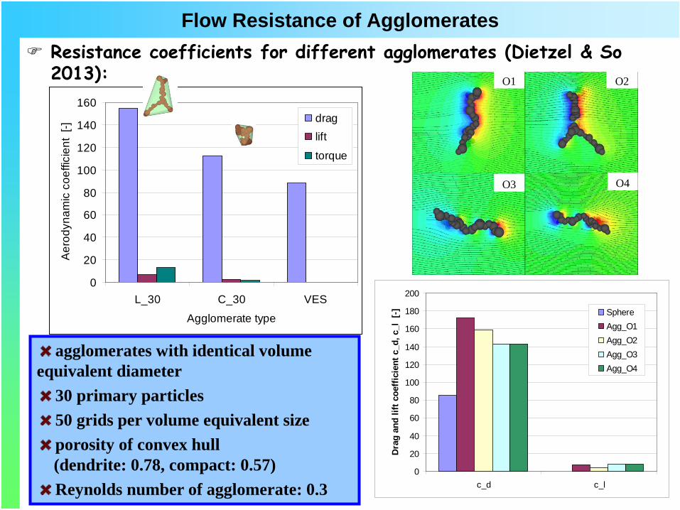
Flow Resistance of Agglomerates Resistance coefficients for different agglomerates (Dietzel & So
2013): O1 O2
O3 O4
0
20
40
60
80
100
120
140
160
L_30 C_30 VES
Agglomerate type
Aer
odyn
amic
coe
ffici
ent
[-]
draglift
torque
0
20
40
60
80
100
120
140
160
180
200
c_d c_l
Dra
g an
d lif
t coe
ffic
ient
c_d
, c_l
[-] Sphere
Agg_O1Agg_O2Agg_O3Agg_O4
agglomerates with identical volume equivalent diameter
30 primary particles 50 grids per volume equivalent size porosity of convex hull
(dendrite: 0.78, compact: 0.57) Reynolds number of agglomerate: 0.3
Martin-Luther-Universität Halle-Wittenberg
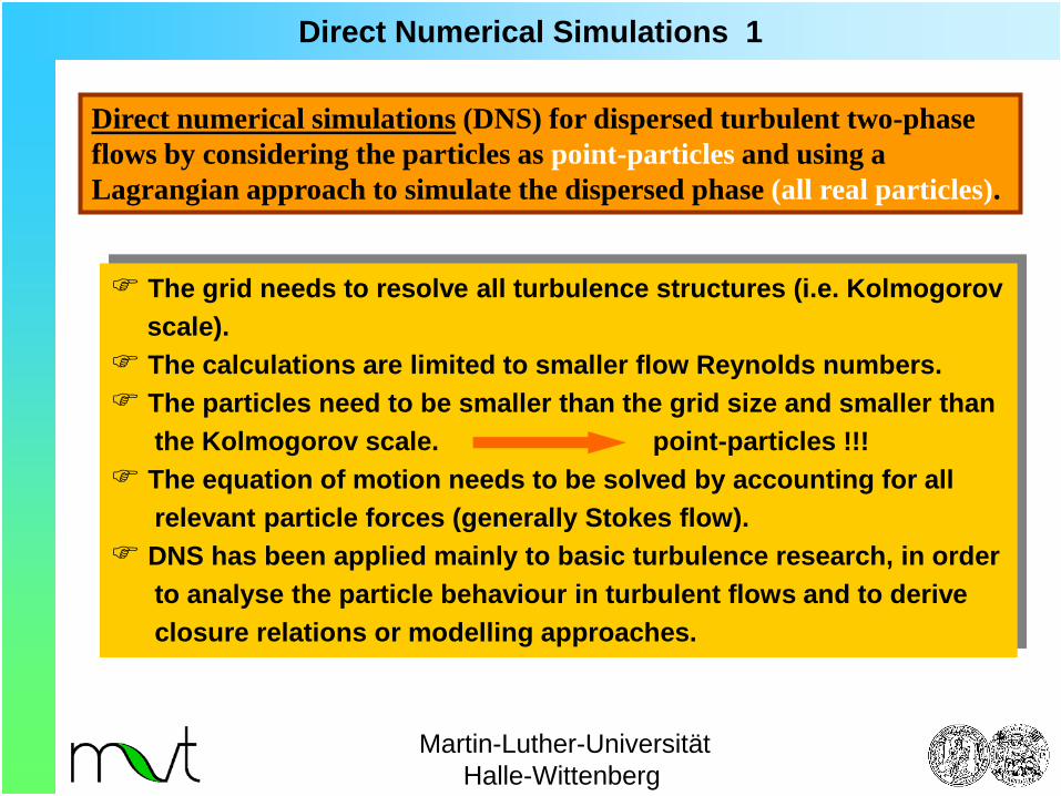
Direct Numerical Simulations 1
Direct numerical simulations (DNS) for dispersed turbulent two-phase flows by considering the particles as point-particles and using a Lagrangian approach to simulate the dispersed phase (all real particles).
The grid needs to resolve all turbulence structures (i.e. Kolmogorov scale). The calculations are limited to smaller flow Reynolds numbers. The particles need to be smaller than the grid size and smaller than the Kolmogorov scale. point-particles !!! The equation of motion needs to be solved by accounting for all relevant particle forces (generally Stokes flow). DNS has been applied mainly to basic turbulence research, in order to analyse the particle behaviour in turbulent flows and to derive closure relations or modelling approaches.
Martin-Luther-Universität Halle-Wittenberg
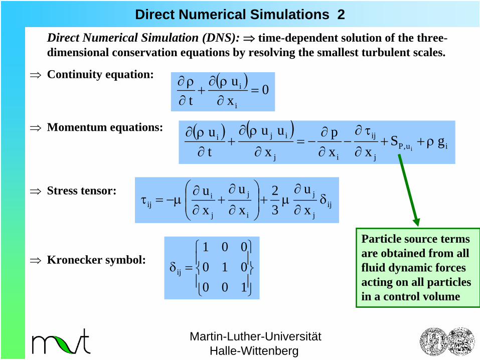
Direct Numerical Simulations 2 Direct Numerical Simulation (DNS): ⇒ time-dependent solution of the three-
dimensional conservation equations by resolving the smallest turbulent scales.
⇒ Continuity equation:
⇒ Momentum equations:
⇒ Stress tensor:
⇒ Kronecker symbol:
( ) 0xu
t i
i =∂ρ∂
+∂
ρ∂
( ) ( )iu,P
j
ij
ij
iji gSxx
px
uutu
iρ++
∂
τ∂−
∂∂
−=∂
ρ∂+
∂ρ∂
ijj
j
i
j
j
iij x
u32
xu
xu
δ∂
∂µ+
∂
∂+
∂∂
−µ=τ
=δ
100010001
ij
Particle source terms are obtained from all fluid dynamic forces acting on all particles in a control volume

Martin-Luther-Universität Halle-Wittenberg
Direct Numerical Simulations 3 Direct numerical simulations (963) on
turbulence modification by particles in isotropic turbulence (Bovin et al. 1998):
( ) 38.11,49.4,26.1/
10/T
m02.0L62Re
0KF12
KE
f
=ττ
=τ
==
=φ
λ
Turbulent kinetic energy
Dissipation rate Particle dissipation
St St
Martin-Luther-Universität Halle-Wittenberg
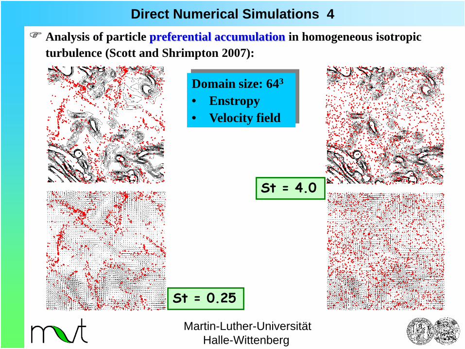
Direct Numerical Simulations 4 Analysis of particle preferential accumulation in homogeneous isotropic
turbulence (Scott and Shrimpton 2007):
Domain size: 643
• Enstropy • Velocity field
St = 0.25
St = 4.0
Martin-Luther-Universität Halle-Wittenberg
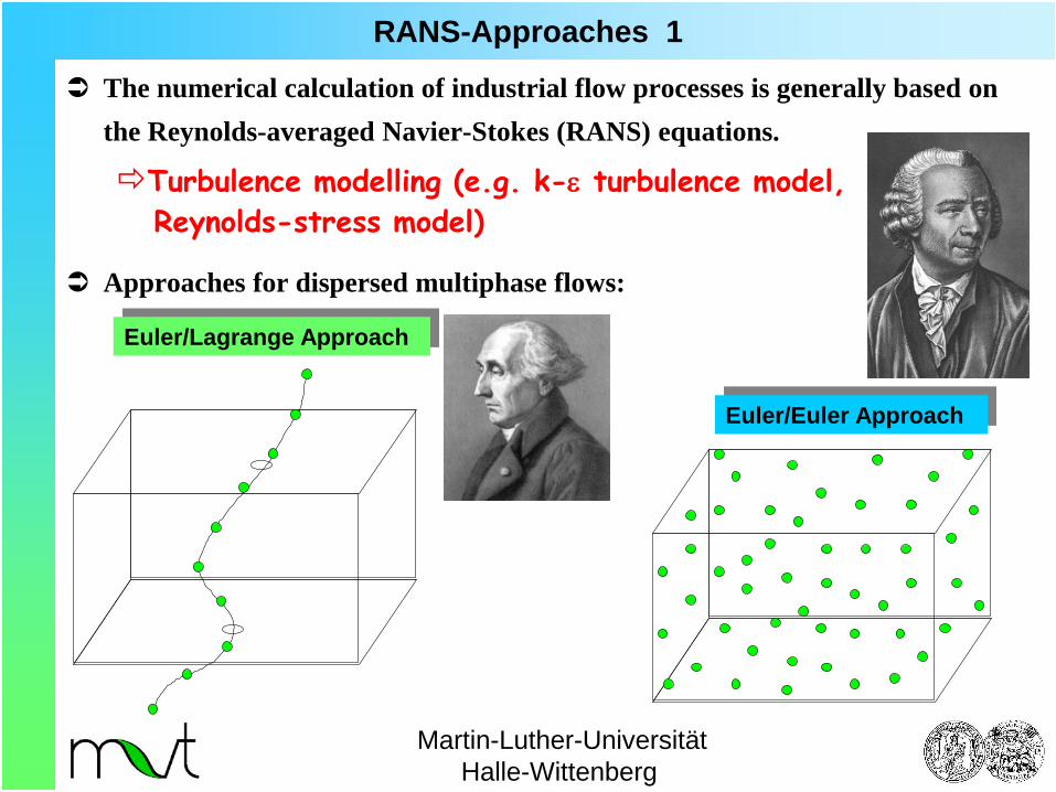
RANS-Approaches 1
The numerical calculation of industrial flow processes is generally based on the Reynolds-averaged Navier-Stokes (RANS) equations.
Turbulence modelling (e.g. k-ε turbulence model, Reynolds-stress model)
Approaches for dispersed multiphase flows:
Euler/Euler Approach
Euler/Lagrange Approach
Martin-Luther-Universität Halle-Wittenberg
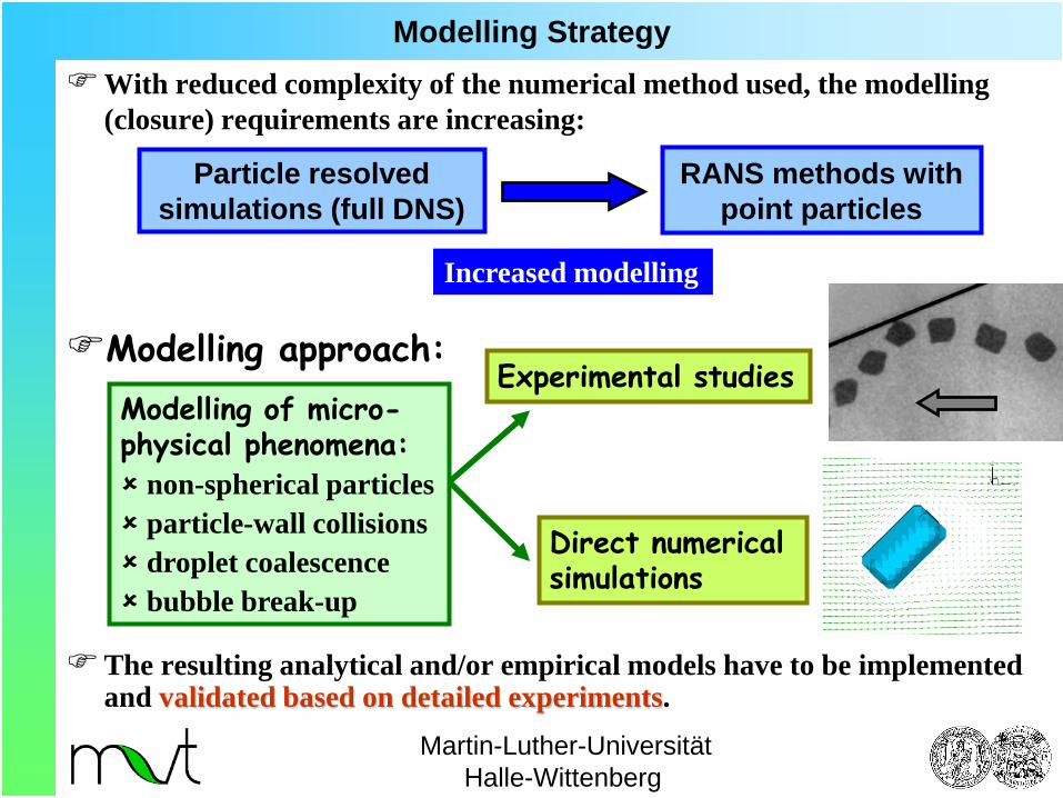
Modelling Strategy With reduced complexity of the numerical method used, the modelling
(closure) requirements are increasing:
Modelling approach:
The resulting analytical and/or empirical models have to be implemented and validated based on detailed experiments.
Particle resolved simulations (full DNS)
RANS methods with point particles
Modelling of micro-physical phenomena: non-spherical particles particle-wall collisions droplet coalescence bubble break-up
Experimental studies
Direct numerical simulations
Increased modelling
Martin-Luther-Universität Halle-Wittenberg
Two-Fluid Approach 1
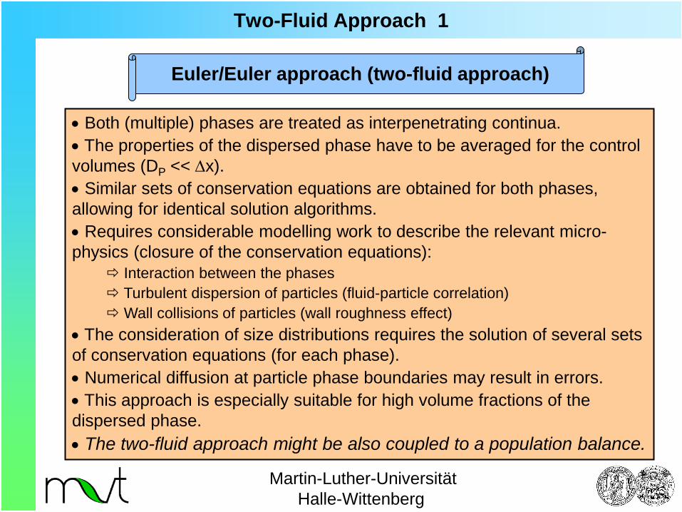
• Both (multiple) phases are treated as interpenetrating continua. • The properties of the dispersed phase have to be averaged for the control volumes (DP << ∆x). • Similar sets of conservation equations are obtained for both phases, allowing for identical solution algorithms. • Requires considerable modelling work to describe the relevant micro-physics (closure of the conservation equations):
Interaction between the phases Turbulent dispersion of particles (fluid-particle correlation) Wall collisions of particles (wall roughness effect)
• The consideration of size distributions requires the solution of several sets of conservation equations (for each phase). • Numerical diffusion at particle phase boundaries may result in errors. • This approach is especially suitable for high volume fractions of the dispersed phase. • The two-fluid approach might be also coupled to a population balance.
Euler/Euler approach (two-fluid approach)
Martin-Luther-Universität Halle-Wittenberg
Two-Fluid Approach 2
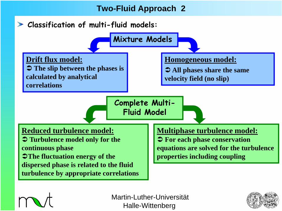
Classification of multi-fluid models:
Mixture Models
Drift flux model: The slip between the phases is calculated by analytical correlations
Homogeneous model: All phases share the same velocity field (no slip)
Complete Multi-Fluid Model
Reduced turbulence model: Turbulence model only for the continuous phase The fluctuation energy of the dispersed phase is related to the fluid turbulence by appropriate correlations
Multiphase turbulence model: For each phase conservation equations are solved for the turbulence properties including coupling
Martin-Luther-Universität Halle-Wittenberg
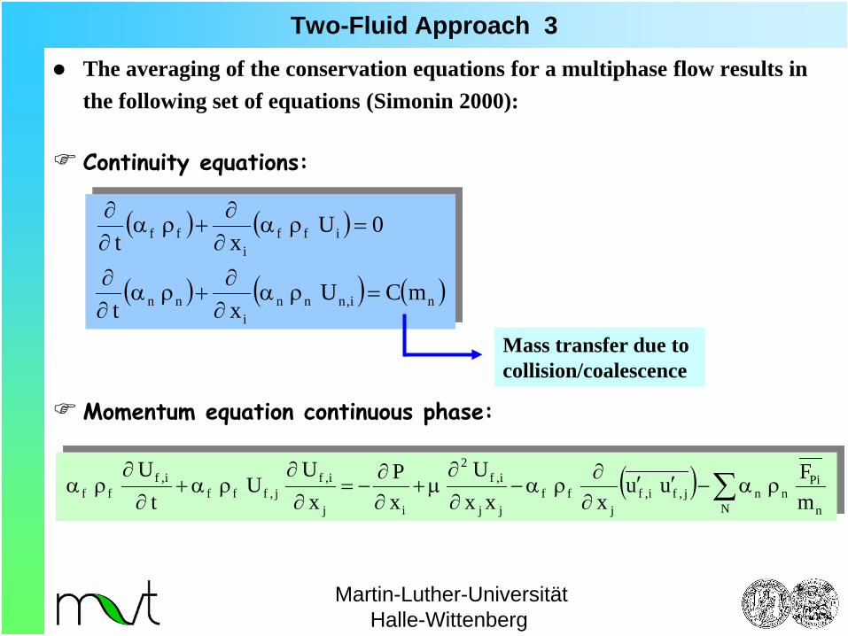
Two-Fluid Approach 3 The averaging of the conservation equations for a multiphase flow results in
the following set of equations (Simonin 2000):
Continuity equations:
Momentum equation continuous phase:
( ) ( )
( ) ( ) ( )ni,nnni
nn
iffi
ff
mCUxt
0Uxt
=ρα∂∂
+ρα∂∂
=ρα∂∂
+ρα∂∂
( ) ∑ ρα−′′∂
∂ρα−
∂∂
µ+∂∂
−=∂
∂ρα+
∂∂
ραN n
Pinnj,fi,f
jff
jj
i,f2
ij
i,fj,fff
i,fff m
Fuuxxx
UxP
xU
Ut
U
Mass transfer due to collision/coalescence
Martin-Luther-Universität Halle-Wittenberg
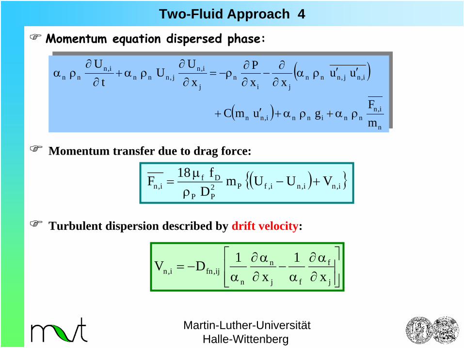
Two-Fluid Approach 4
Momentum equation dispersed phase:
Momentum transfer due to drag force:
Turbulent dispersion described by drift velocity:
( )
( )n
i,nnninni,nn
i,nj,nnnji
nj
i,nj,nnn
i,nnn
mF
gumC
uuxx
Px
UU
tU
ρα+ρα+′+
′′ρα∂
∂−
∂∂
ρ−=∂
∂ρα+
∂∂
ρα
( ) i,ni,ni,fP2PP
Dfi,n VUUm
Df18F +−
ρµ
=
∂α∂
α−
∂α∂
α−=
j
f
fj
n
nij,fni,n x
1x
1DV
Martin-Luther-Universität Halle-Wittenberg
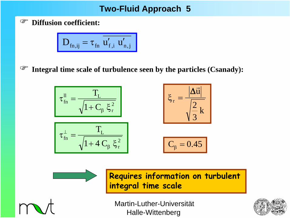
Two-Fluid Approach 5 Diffusion coefficient:
Integral time scale of turbulence seen by the particles (Csanady):
j,ni,ffnij,fn uuD ′′τ=
2r
Lllfn
C1T
ξ+=τ
β
2r
Lfn
C41T
ξ+=τ
β
⊥
k32u
r
∆
=ξ
45.0C =β
Requires information on turbulent integral time scale
Martin-Luther-Universität Halle-Wittenberg
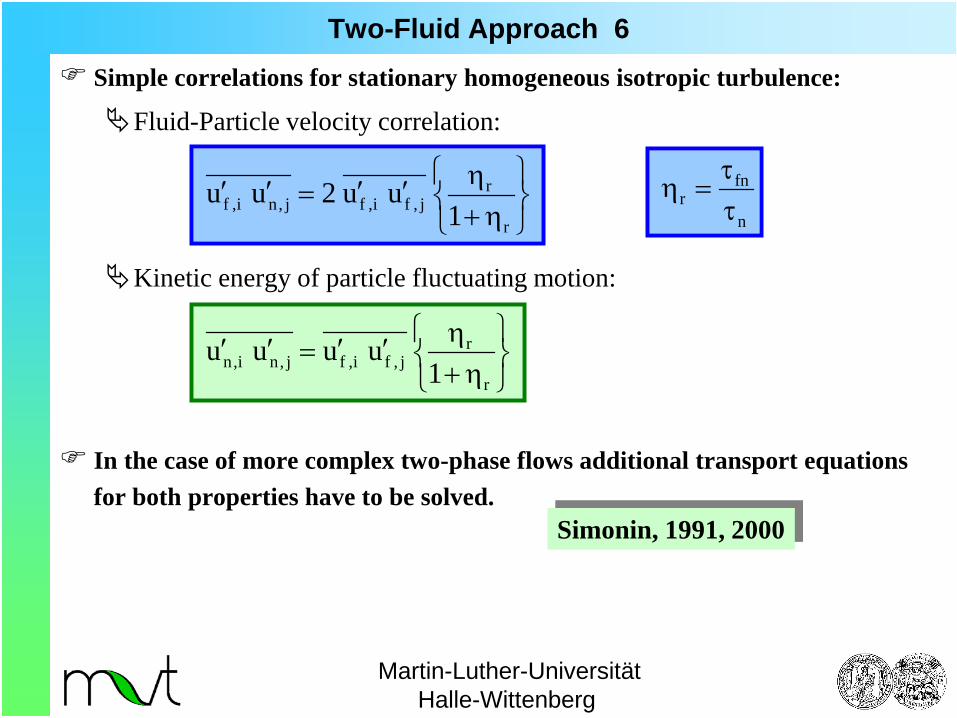
Two-Fluid Approach 6 Simple correlations for stationary homogeneous isotropic turbulence:
Fluid-Particle velocity correlation:
Kinetic energy of particle fluctuating motion:
In the case of more complex two-phase flows additional transport equations for both properties have to be solved.
η+η′′=′′
r
rj,fi,fj,ni,f 1
uu2uu
η+η′′=′′
r
rj,fi,fj,ni,n 1
uuuu
n
fnr τ
τ=η
Simonin, 1991, 2000
Martin-Luther-Universität Halle-Wittenberg
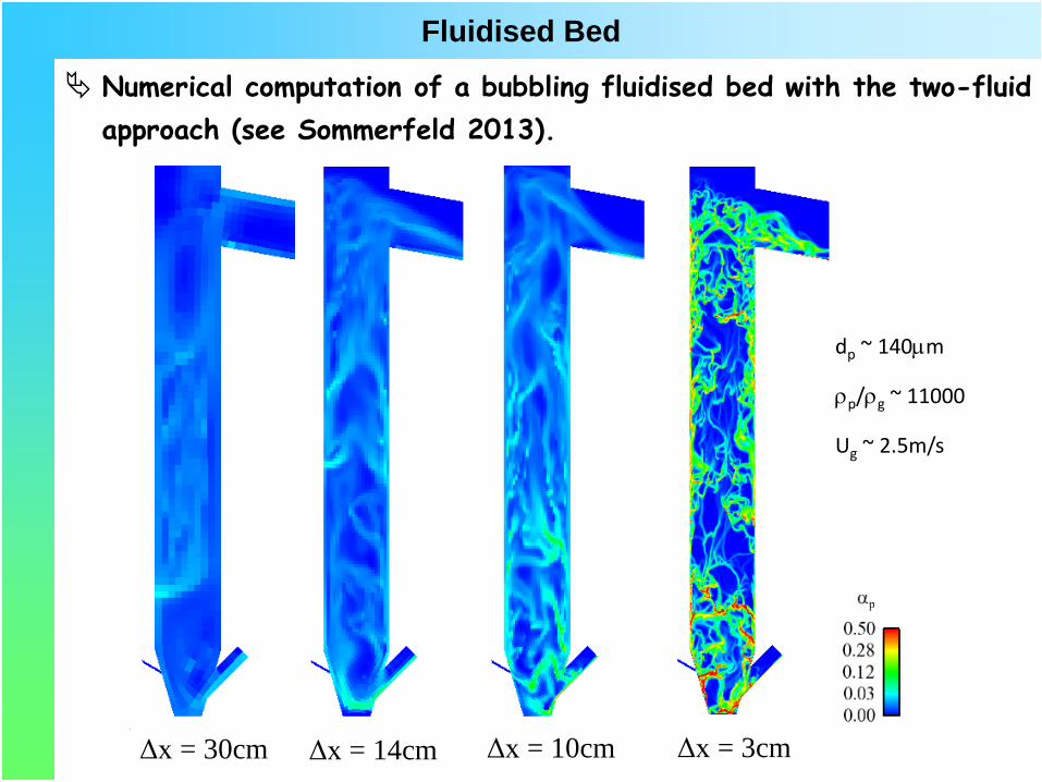
Fluidised Bed
Numerical computation of a bubbling fluidised bed with the two-fluid approach (see Sommerfeld 2013).
dp ~ 140µm
ρp/ρg ~ 11000
Ug ~ 2.5m/s
Δx = 30cm Δx = 14cm Δx = 10cm Δx = 3cm
Martin-Luther-Universität Halle-Wittenberg
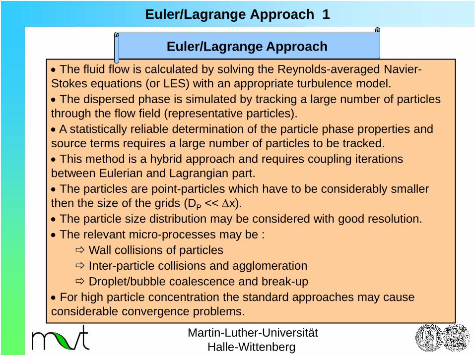
Euler/Lagrange Approach 1
• The fluid flow is calculated by solving the Reynolds-averaged Navier-Stokes equations (or LES) with an appropriate turbulence model. • The dispersed phase is simulated by tracking a large number of particles through the flow field (representative particles). • A statistically reliable determination of the particle phase properties and source terms requires a large number of particles to be tracked. • This method is a hybrid approach and requires coupling iterations between Eulerian and Lagrangian part. • The particles are point-particles which have to be considerably smaller then the size of the grids (DP << ∆x). • The particle size distribution may be considered with good resolution. • The relevant micro-processes may be : Wall collisions of particles Inter-particle collisions and agglomeration Droplet/bubble coalescence and break-up
• For high particle concentration the standard approaches may cause considerable convergence problems.
Euler/Lagrange Approach
Martin-Luther-Universität Halle-Wittenberg
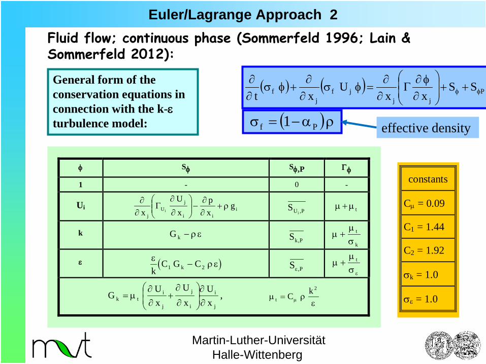
Euler/Lagrange Approach 2 Fluid flow; continuous phase (Sommerfeld 1996; Lain &
Sommerfeld 2012):
constants
Cµ = 0.09
C1 = 1.44
C2 = 1.92
σk = 1.0
σε = 1.0
φ Sφ Sφ,P Γφ
1 - 0 -
Ui iii
jU
j
gxp
xU
x iρ+
∂∂
−
∂
∂Γ
∂∂
P,UiS tµ+µ
k G k − ρεP,kS µ
µσ
+ t
k
ε ( )ερε
kC G Ck1 2−
P,Sεµ
µσ ε
+ t
j
i
i
j
j
itk x
UxU
xU
G∂∂
∂
∂+
∂∂
µ= , ε
ρ=µ µ
2
tkC
General form of the conservation equations in connection with the k-ε turbulence model:
( ) ( ) Pjj
jfj
f SSxx
Uxt φφ ++
∂φ∂
Γ∂
∂=φσ
∂∂
+φσ∂∂
( )ρα−=σ Pf 1 effective density
Martin-Luther-Universität Halle-Wittenberg
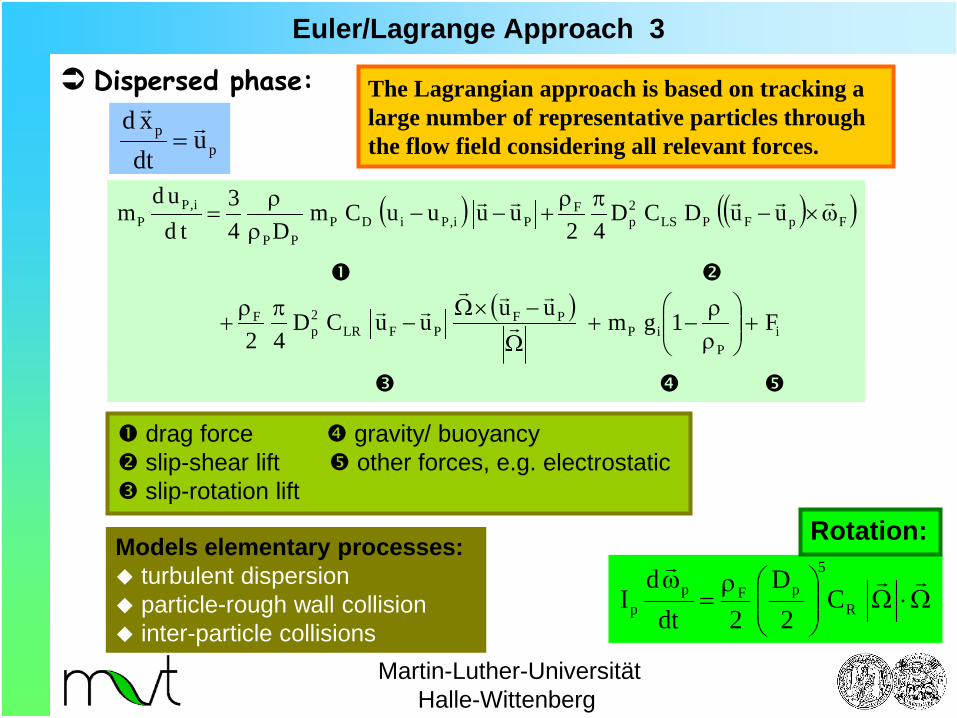
Euler/Lagrange Approach 3
Dispersed phase:
( ) ( )( )
( )i
PiP
PFPFLR
2p
F
FpFPLS2p
FPi,PiDP
PP
i,PP
F1gmuuuuCD42
uuDCD42
uuuuCmD4
3td
udm
+
ρρ
−+Ω
−×Ω−
πρ+
ω×−πρ
+−−ρ
ρ=
The Lagrangian approach is based on tracking a large number of representative particles through the flow field considering all relevant forces.
drag force gravity/ buoyancy slip-shear lift other forces, e.g. electrostatic slip-rotation lift
Ω⋅Ω
ρ=
ω
R
5pFp
p C2
D2dt
dI
Rotation:
pp u
dtxd
=
Models elementary processes: turbulent dispersion particle-rough wall collision inter-particle collisions
Martin-Luther-Universität Halle-Wittenberg
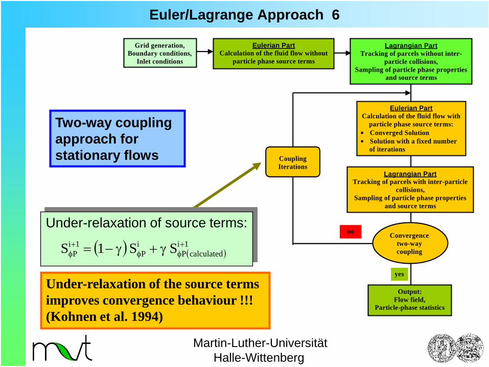
Euler/Lagrange Approach 6
Two-way coupling approach for stationary flows
Eulerian Part
Calculation of the fluid flow without particle phase source terms
Eulerian Part Calculation of the fluid flow with
particle phase source terms: • Converged Solution • Solution with a fixed number
of iterations
yes
Output: Flow field,
Particle-phase statistics
no
Grid generation, Boundary conditions,
Inlet conditions
Lagrangian Part Tracking of parcels without inter-
particle collisions, Sampling of particle phase properties
and source terms
Lagrangian Part Tracking of parcels with inter-particle
collisions, Sampling of particle phase properties
and source terms
Convergence two-way coupling
Coupling Iterations
Under-relaxation of the source terms improves convergence behaviour !!! (Kohnen et al. 1994)
Under-relaxation of source terms:
( ) ( )1i
calculatedPi
P1i
P SS1S +φφ
+φ γ+γ−=
Martin-Luther-Universität Halle-Wittenberg
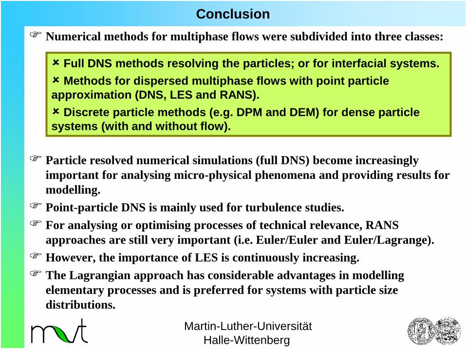
Conclusion Numerical methods for multiphase flows were subdivided into three classes:
Particle resolved numerical simulations (full DNS) become increasingly
important for analysing micro-physical phenomena and providing results for modelling.
Point-particle DNS is mainly used for turbulence studies. For analysing or optimising processes of technical relevance, RANS
approaches are still very important (i.e. Euler/Euler and Euler/Lagrange). However, the importance of LES is continuously increasing. The Lagrangian approach has considerable advantages in modelling
elementary processes and is preferred for systems with particle size distributions.
Full DNS methods resolving the particles; or for interfacial systems. Methods for dispersed multiphase flows with point particle approximation (DNS, LES and RANS). Discrete particle methods (e.g. DPM and DEM) for dense particle systems (with and without flow).
Related Documents