Review Genetic analysis of longitudinal data in beef ... · Review Genetic analysis of longitudinal data in beef ... Department of Animal Sciences, Colorado State University, Fort

©FUNPEC-RP www.funpecrp.com.brGenetics and Molecular Research 9 (1): 19-33 (2010)

Review

Genetic analysis of longitudinal data in beef cattle: a review

S.E. Speidel, R.M. Enns and D.H. Crews Jr.

Department of Animal Sciences, Colorado State University,Fort Collins, CO, USA

Corresponding author: S.E. SpeidelE-mail: [email protected]

Genet. Mol. Res. 9 (1): 19-33 (2010)Received September 21, 2009Accepted December 15, 2009Published January 5, 2010

ABSTRACT. Currently, many different data types are collected by beef cattle breed associations for the purpose of genetic evaluation. These data points are all biological characteristics of individual animals that can be measured multiple times over an animal’s lifetime. Some traits can only be measured once on an individual animal, whereas others, such as the body weight of an animal as it grows, can be measured many times. Data such as growth has been often referred to as “longitudinal” or “infinite-dimensional” since it is theoretically possible to observe the trait an infinite number of times over the life span of a given individual. Analysis of such data is not without its challenges, and as a result many different methods have been or are beginning to be implemented in the genetic analysis of beef cattle data, each an improvement over its predecessor. These methods of analysis range from the classic repeated measures to the more contemporary suite of random regressions that use covariance functions or even splines as their base function. Each of the approaches has both strengths and weaknesses in the analysis of longitudinal data. Here we summarize past and current genetic evaluation technology for analyzing this type of data and review some emerging technologies beginning to be implemented in national cattle evaluation schemes, along with their potential implications for the beef industry.

Key words: Beef cattle; Longitudinal data; Random regression;Genetic evaluation

20


S.E. Speidel et al.

INTRODUCTION

In today’s beef industry, many different data types are collected by beef cattle breed as-sociations for the purpose of genetic evaluation. These data points are all biological characteristics of individual animals that can be measured many times over an animal’s lifetime. The number of times a given trait is observed during an animal’s life is dictated by the nature of the trait. For example, traits such as carcass characteristics, heifer calving ease, and heifer pregnancy can only be recorded once on an individual animal. However, traits that monitor the status of an animal as it grows, such as weight traits and live animal indicators of carcass merit can be measured a number of times over the life span of an animal. Weight traits such as birth weight and weaning weight de-scribe the same underlying trait, which is growth as measured by weight gain observed over time. As such, perhaps they can be best described by some type of mathematical function rather than a finite set of data points (Kirkpatrick and Heckman, 1989; Meyer and Kirkpatrick, 2005). Conse-quently, this unique type of data has been referred to throughout the literature as “function valued” (Kirkpatrick and Heckman, 1989; Meyer and Kirkpatrick, 2005) or as “infinite-dimensional” and “longitudinal” data by Meyer and Hill (1997). Here we summarize past and current genetic evalu-ation technology for handling longitudinal data, and discuss some emerging technologies that are beginning to be implemented in national cattle evaluation schemes.

LONGITUDINAL DATA

A number of traits currently collected for beef cattle genetic evaluation fall under the umbrella definition of longitudinal data. These traits can range from commonly col-lected observations, such as weight, height and body condition score measurements, to more obscure measures such as feed intake, survival and sperm production and quality (Schaeffer, 2004). Several different methods have been implemented by groups conduct-ing national cattle evaluations to properly model these data types. These methods include more traditional models, such as repeatability and multivariate models, to more contem-porary (and perhaps more appropriate) models, such as the suite of random regression models using different base functions (Mrode, 2005).

Analysis of function-valued traits is challenging, and each of the different methods has their respective benefits and limitations. Discussion of these benefits and limitations for each of the methods of analysis will be addressed individually, beginning with the traditional repeatability model, then on to the multivariate models and finally finishing with random re-gression models that use covariance functions and splines as their base function.

THE REPEATABILITY MODEL

Perhaps the simplest method of analysis of longitudinal data is the “Repeatability Model”. The idea behind this model is to treat each observation as a repeated record of the same trait on the same individual. This model has been implemented in the past for traits such as litter size in successive pregnancies in swine and milk yield in successive lactations in dairy cattle (Jamrozik et al., 1997b; Interbull, 2000).

The repeatability model is most often described in matrix form by the equation (Mrode, 2005)

21


Analysis of longitudinal data in beef cattle

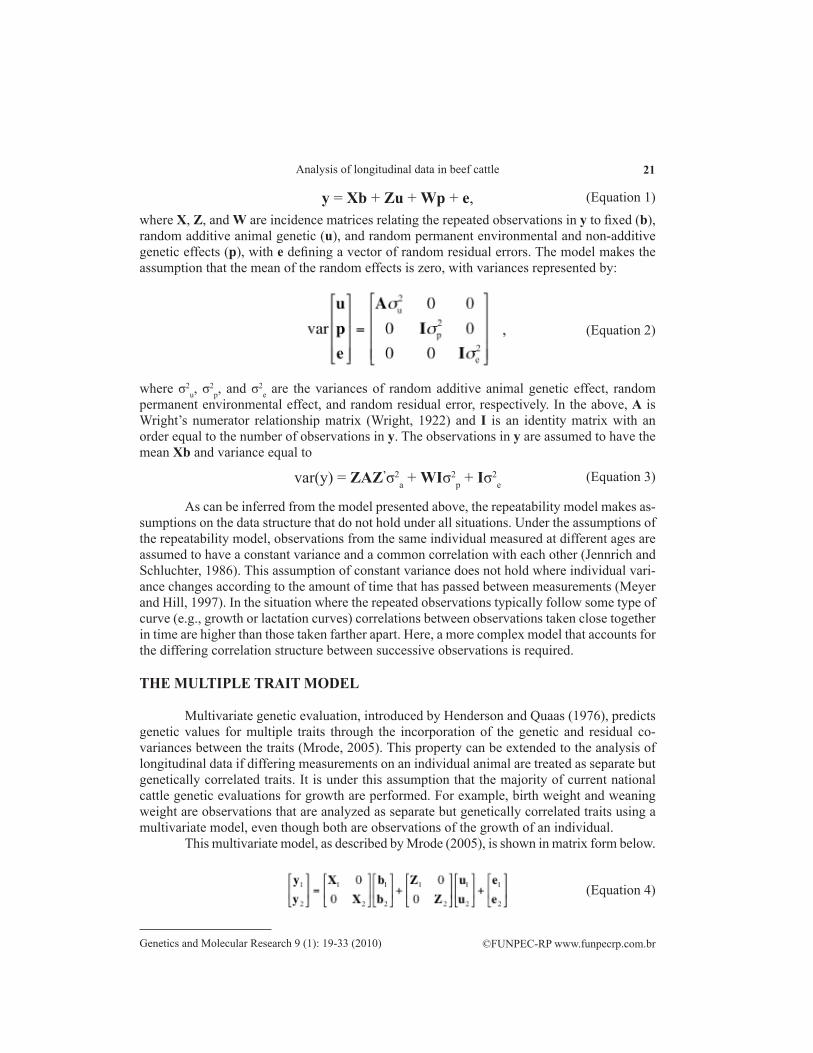
where X, Z, and W are incidence matrices relating the repeated observations in y to fixed (b), random additive animal genetic (u), and random permanent environmental and non-additive genetic effects (p), with e defining a vector of random residual errors. The model makes the assumption that the mean of the random effects is zero, with variances represented by:

y = Xb + Zu + Wp + e, (Equation 1)

, (Equation 2)

where σ2u, σ

2p, and σ2

e are the variances of random additive animal genetic effect, random permanent environmental effect, and random residual error, respectively. In the above, A is Wright’s numerator relationship matrix (Wright, 1922) and I is an identity matrix with an order equal to the number of observations in y. The observations in y are assumed to have the mean Xb and variance equal to

var(y) = ZAZ’σ2a + WIσ2

p + Iσ2e

As can be inferred from the model presented above, the repeatability model makes as-sumptions on the data structure that do not hold under all situations. Under the assumptions of the repeatability model, observations from the same individual measured at different ages are assumed to have a constant variance and a common correlation with each other (Jennrich and Schluchter, 1986). This assumption of constant variance does not hold where individual vari-ance changes according to the amount of time that has passed between measurements (Meyer and Hill, 1997). In the situation where the repeated observations typically follow some type of curve (e.g., growth or lactation curves) correlations between observations taken close together in time are higher than those taken farther apart. Here, a more complex model that accounts for the differing correlation structure between successive observations is required.

THE MULTIPLE TRAIT MODEL

Multivariate genetic evaluation, introduced by Henderson and Quaas (1976), predicts genetic values for multiple traits through the incorporation of the genetic and residual co-variances between the traits (Mrode, 2005). This property can be extended to the analysis of longitudinal data if differing measurements on an individual animal are treated as separate but genetically correlated traits. It is under this assumption that the majority of current national cattle genetic evaluations for growth are performed. For example, birth weight and weaning weight are observations that are analyzed as separate but genetically correlated traits using a multivariate model, even though both are observations of the growth of an individual.

This multivariate model, as described by Mrode (2005), is shown in matrix form below.

(Equation 3)

(Equation 4)

22


S.E. Speidel et al.

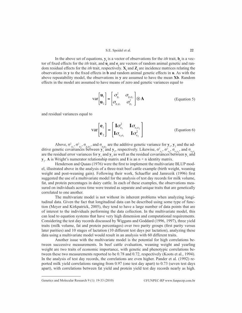
In the above set of equations, yi is a vector of observations for the ith trait, bi is a vec-tor of fixed effects for the ith trait, and ui and ei are vectors of random animal genetic and ran-dom residual effects for the ith trait, respectively. Xi and Zi are incidence matrices relating the observations in y to the fixed effects in b and random animal genetic effects in u. As with the above repeatability model, the observations in y are assumed to have the mean Xb. Random effects in the model are assumed to have means of zero and genetic variances equal to

(Equation 5)

and residual variances equal to

Above, σ2g1

, σ2g2

, σg1g2, and σg2g1

are the additive genetic variance for y1, y2 and the ad-ditive genetic covariances between y1 and y2, respectively. Likewise, σ2

e1, σ2

e2, σe1e2

, and σe2e1 are the residual error variances for y1 and y2 as well as the residual covariances between y1 and y2. A is Wright’s numerator relationship matrix and I is an n × n identity matrix.

Henderson and Quaas (1976) were the first to implement the multivariate BLUP mod-el, illustrated above in the analysis of a three-trait beef cattle example (birth weight, weaning weight and post-weaning gain). Following their work, Schaeffer and Jamrozik (1996) first suggested the use of a multivariate model for the analysis of test day records for milk volume, fat, and protein percentages in dairy cattle. In each of these examples, the observations mea-sured on individuals across time were treated as separate and unique traits that are genetically correlated to one another.

The multivariate model is not without its inherent problems when analyzing longi-tudinal data. Given the fact that longitudinal data can be described using some type of func-tion (Meyer and Kirkpatrick, 2005), they tend to have a large number of data points that are of interest to the individuals performing the data collection. In the multivariate model, this can lead to equation systems that have very high dimension and computational requirements. Considering the test day records discussed by Wiggans and Goddard (1996, 1997), three yield traits (milk volume, fat and protein percentages) over two parity groups (first parity versus later parities) and 10 stages of lactation (10 different test days per lactation), analyzing these data using a multivariate model would result in an analysis with 60 different traits.

Another issue with the multivariate model is the potential for high correlations be-tween successive measurements. In beef cattle evaluation, weaning weight and yearling weight are two traits of economic importance, with genetic and phenotypic correlations be-tween these two measurements reported to be 0.78 and 0.72, respectively (Koots et al., 1994). In the analysis of test day records, the correlations are even higher. Pander et al. (1992) re-ported milk yield correlations ranging from 0.97 (one test day apart) to 0.73 (seven test days apart), with correlations between fat yield and protein yield test day records nearly as high.

(Equation 6)

23



These elevated correlations are undesirable for two main reasons. First, if two variables pre-dict the same information, it does not make sense to include both of the variables in the model. Second, the correlation between the two variables has the effect of reducing the power of the tests of significance (Foster et al., 2006).

The high correlations between traits such as weaning and yearling weights as well as between individual test days in dairy cattle evaluation have resulted in studies designed to determine how to specifically handle these elevated correlations. One method, an exten-sion of the multivariate model, allows higher correlations between observations measured close together than those measured farther apart. This technique, referred to as autoregression or autocorrelation, has been documented in the literature numerous times (Harville, 1979; Kachman and Everett, 1993; Carvalheira et al., 1998). Another method to handle this data type is to model the data using a pre-determined function, or data mean. Referred to as fixed regres-sion (Mrode, 2005), these functions can be extended in such a manner that each individual will have its own random function.

RANDOM REGRESSION

Regression models have been used in the analysis of longitudinal data for many years. The use of pre-determined functions as covariates was introduced as random regression or a random coefficient model during the early to the mid 1980’s (Henderson Jr., 1982; Laird and Ware, 1982; Jennrich and Schluchter, 1986). However, the first study with application to live-stock production data was conducted by Ptak and Schaeffer (1993) in the analysis of test day milk production records of dairy cattle. This first attempt was not a random regression model, but it accounted for the general shape or mean lactation curve for cows within similar herd, year and season. Following this initial trial, Schaeffer et al. (1994) extended the regression coefficients of this fixed regression model to random animal effects. In doing so, they were able to account for the mean shape of the lactation curve within a given herd, year and sea-son, as well as account for the deviation of each individual animal’s lactation curve from this mean shape. They were also able to account for the change in correlation structure of repeated records on individuals over time. This ability of the random regression model to properly ac-count for the changing correlation structure has been shown to result in an increase in predic-tion accuracy of 5.9% when compared to the multivariate model (Meyer, 2004).

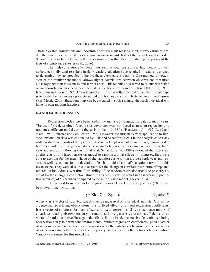
The general form of a random regression model, as described by Mrode (2005), can be shown in matrix form as

(Equation 7)y = Xb + Qu + Zpe + e

where y is a vector of repeated test day yields measured on individual animals, X is an in-cidence matrix relating observations in y to fixed effects and fixed regression coefficients, b is a vector of solutions for fixed effects and fixed regressions, Q is an incidence matrix of covariates relating observations in y to random additive genetic regression coefficients, u is a vector of random additive direct genetic effects, Z is an incidence matrix of covariates relating observations in y to permanent environmental random regression coefficients, pe is a vector of random permanent environmental regression coefficients for each animal, and e is a vector of random residuals that includes the temporary environmental effects for each observation. Variances assumed for this model are

24


S.E. Speidel et al.

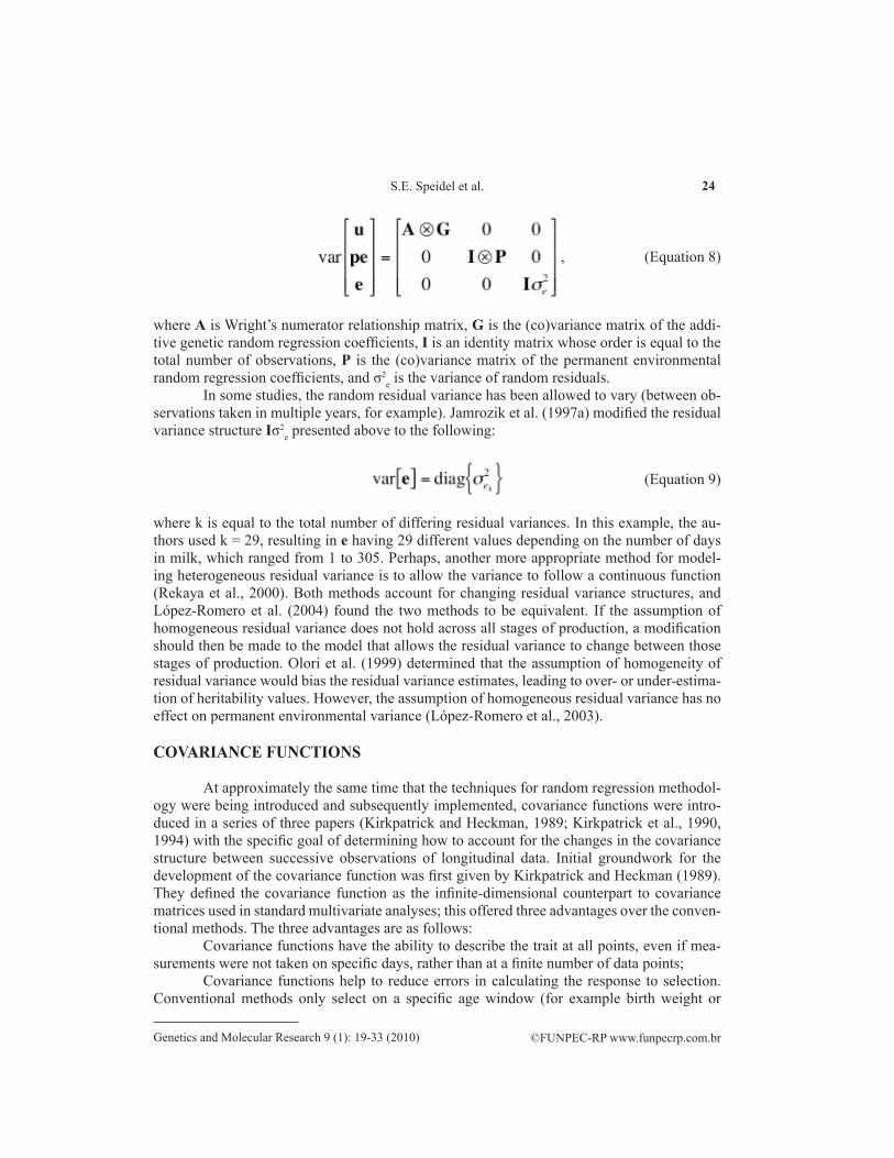
where A is Wright’s numerator relationship matrix, G is the (co)variance matrix of the addi-tive genetic random regression coefficients, I is an identity matrix whose order is equal to the total number of observations, P is the (co)variance matrix of the permanent environmental random regression coefficients, and σ2

e is the variance of random residuals. In some studies, the random residual variance has been allowed to vary (between ob-

servations taken in multiple years, for example). Jamrozik et al. (1997a) modified the residual variance structure Iσ2

e presented above to the following:

, (Equation 8)

where k is equal to the total number of differing residual variances. In this example, the au-thors used k = 29, resulting in e having 29 different values depending on the number of days in milk, which ranged from 1 to 305. Perhaps, another more appropriate method for model-ing heterogeneous residual variance is to allow the variance to follow a continuous function (Rekaya et al., 2000). Both methods account for changing residual variance structures, and López-Romero et al. (2004) found the two methods to be equivalent. If the assumption of homogeneous residual variance does not hold across all stages of production, a modification should then be made to the model that allows the residual variance to change between those stages of production. Olori et al. (1999) determined that the assumption of homogeneity of residual variance would bias the residual variance estimates, leading to over- or under-estima-tion of heritability values. However, the assumption of homogeneous residual variance has no effect on permanent environmental variance (López-Romero et al., 2003).

COVARIANCE FUNCTIONS

At approximately the same time that the techniques for random regression methodol-ogy were being introduced and subsequently implemented, covariance functions were intro-duced in a series of three papers (Kirkpatrick and Heckman, 1989; Kirkpatrick et al., 1990, 1994) with the specific goal of determining how to account for the changes in the covariance structure between successive observations of longitudinal data. Initial groundwork for the development of the covariance function was first given by Kirkpatrick and Heckman (1989). They defined the covariance function as the infinite-dimensional counterpart to covariance matrices used in standard multivariate analyses; this offered three advantages over the conven-tional methods. The three advantages are as follows:

Covariance functions have the ability to describe the trait at all points, even if mea-surements were not taken on specific days, rather than at a finite number of data points;

Covariance functions help to reduce errors in calculating the response to selection. Conventional methods only select on a specific age window (for example birth weight or

(Equation 9)

25



weaning weight); however, when selection on a part of the curve is performed, the entire trajectory is changed through the genetic correlation (selecting on increasing birth weight has the correlated effect of increasing weaning weight). Covariance functions help account for the correlated responses observed at other data points as well;

Covariance functions estimate parameters more efficiently, due simply to the fact that more data points are used in the analysis.

Kirkpatrick et al. (1990, 1994) provided additional insight into the covariance func-tion they introduced in 1989, with examples from a beef cattle growth data set. Calculating the covariance function begins with the standard classical quantitative genetic (co)variance matrix of the traits in question over different times, often referred to as G (see the multivariate model presented above). Using a beef cattle growth analysis as an example, the genetic (co)variance matrix (G) could consist of the additive genetic variance for birth weight and wean-ing weight. Using this G, covariance functions are built by using a smooth curve to interpolate the values of G between the measured ages (birth weight and weaning weight). The process starts with the decision as to which smooth curve to use. Kirkpatrick et al. (1990) suggest the use of Legendre polynomials, but state that any orthogonal function could in fact be used. For longitudinal data such as growth, the authors favored polynomials because growth tends to be smooth, similar to the curves created using polynomial functions.

A number of sources illustrate the calculation of Legendre polynomial functions. The equations presented here were adapted from Schaeffer (2003). To calculate Legendre poly-nomials, first we need to define the polynomials P0(x) = 1, and P1(x) = x. Then, additional polynomials can be calculated using the recursive formula:

Once calculated, these values are then normalized using:

(Equation 10)

Table 1 illustrates how a fourth-order polynomial would be calculated using the above equations for a normalized Legendre polynomial. This series of normalized polynomials (fn(x)) shown in Table 1 are then placed into a matrix Λ such that

(Equation 11)

(Equation 12)

26


S.E. Speidel et al.

Legendre polynomials are defined over the interval of -1 to 1 (Kirkpatrick et al., 1990), therefore it is necessary to standardize the ages of the observations to the interval of -1 and 1. The formula used to standardize these ages was presented by Schaeffer (2003) and is defined as follows

Order Legendre polynomial Normalized Legendre polynomial

N = 0

N = 1

N = 2

N = 3

N = 4

Table 1. Normalized Legendre polynomials for up to a fourth-order polynomial.

where t*i is the standardized time, ti is the time point being standardized, and tmin and tmax were

the minimum and maximum time points or ages represented in the dataset, respectively. Stan-dardized time values are placed into a matrix M, such that an example standardized age vector

(Equation 13)

would result in

(Equation 14)

for a quadratic polynomial. The first column of the matrix is a column of ones representing the intercept of the curve; the second column is the standardized age, while the third column is the standardized age squared for the quadratic term. Fitting higher order polynomials is done by the addition of columns for the additional parameters needed. The next step is to combine the standardized ages and the polynomials into a matrix Φ = MΛ. Performing this step with the M defined above and the first three rows (quadratic) of Λ' gives the matrix

(Equation 15)

(Equation 16)

27



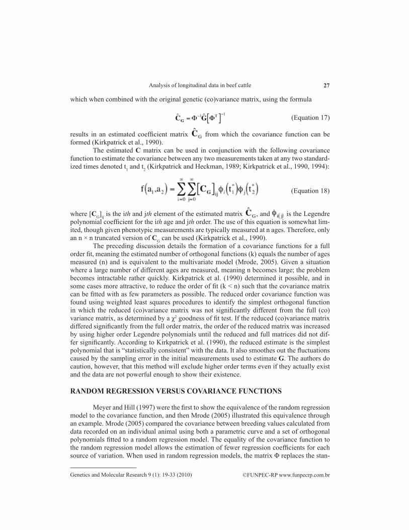
which when combined with the original genetic (co)variance matrix, using the formula

results in an estimated coefficient matrix from which the covariance function can be formed (Kirkpatrick et al., 1990).

The estimated C matrix can be used in conjunction with the following covariance function to estimate the covariance between any two measurements taken at any two standard-ized times denoted t1 and t2 (Kirkpatrick and Heckman, 1989; Kirkpatrick et al., 1990, 1994):

(Equation 17)

where [CG]ij is the ith and jth element of the estimated matrix , and is the Legendre polynomial coefficient for the ith age and jth order. The use of this equation is somewhat lim-ited, though given phenotypic measurements are typically measured at n ages. Therefore, only an n × n truncated version of CG can be used (Kirkpatrick et al., 1990).

The preceding discussion details the formation of a covariance functions for a full order fit, meaning the estimated number of orthogonal functions (k) equals the number of ages measured (n) and is equivalent to the multivariate model (Mrode, 2005). Given a situation where a large number of different ages are measured, meaning n becomes large; the problem becomes intractable rather quickly. Kirkpatrick et al. (1990) determined it possible, and in some cases more attractive, to reduce the order of fit (k < n) such that the covariance matrix can be fitted with as few parameters as possible. The reduced order covariance function was found using weighted least squares procedures to identify the simplest orthogonal function in which the reduced (co)variance matrix was not significantly different from the full (co)variance matrix, as determined by a χ2 goodness of fit test. If the reduced (co)variance matrix differed significantly from the full order matrix, the order of the reduced matrix was increased by using higher order Legendre polynomials until the reduced and full matrices did not dif-fer significantly. According to Kirkpatrick et al. (1990), the reduced estimate is the simplest polynomial that is “statistically consistent” with the data. It also smoothes out the fluctuations caused by the sampling error in the initial measurements used to estimate G. The authors do caution, however, that this method will exclude higher order terms even if they actually exist and the data are not powerful enough to show their existence.

RANDOM REGRESSION VERSUS COVARIANCE FUNCTIONS

Meyer and Hill (1997) were the first to show the equivalence of the random regression model to the covariance function, and then Mrode (2005) illustrated this equivalence through an example. Mrode (2005) compared the covariance between breeding values calculated from data recorded on an individual animal using both a parametric curve and a set of orthogonal polynomials fitted to a random regression model. The equality of the covariance function to the random regression model allows the estimation of fewer regression coefficients for each source of variation. When used in random regression models, the matrix Φ replaces the stan-

(Equation 18)

28


S.E. Speidel et al.

dard covariate incidence matrix.Recently, some issues have surfaced concerning random regression models that em-

ploy Legendre polynomials as their base function. The estimated covariance matrices used to calculate genetic variances over the range of data (over the range of lactation for instance) tend to result in genetic variances that are much higher at the beginning and end of the data range than in the middle (Schaeffer and Jamrozik, 2008). Perhaps this is due to the fact that polynomials place a large amount of emphasis on observations at the extremes, which com-pounds the problem with higher orders of fit (Meyer, 2005a). Other reported problems with Legendre polynomials being used in random regressions are the poor modeling capabilities of asymmetrical functions, their lack of information to estimate a large number of parameters, and their sensitivity to each of the many different (co)variance parameters (Misztal, 2006).

SPLINES

Given the problems with the use of polynomials as a basis function in random regres-sion models discussed by Misztal (2006) and Schaeffer and Jamrozik (2008), several differ-ent alternatives such as fractional polynomials (Robert-Granié et al., 2002), cubic smoothing splines (White et al., 1999), and B-splines (Torres Jr. and Quaas, 2001; Meyer, 2005b) have been proposed. Spline functions are defined as piecewise polynomials that join together at “knots” and are continuous across the range of data (Wold, 1974). As a result, they do not suf-fer from the same problems as polynomials, where their behavior in one small area determines their behavior across the entire range of data. Since splines are defined as “piecewise polyno-mials” they represent smooth curves between each knot.

Ruppert et al. (2003) describes simple spline basis functions as an extension of the following standard simple linear regression model

yi = β0 + β1xi + ei

where yi is the observed value of the ith trial, xi is the predictor variable of the ith trial, b0 and b1 are regression coefficients corresponding to the y intercept and slope of the regression line, respectively, and ei is the random error term with mean equal to 0 and variance equal to σ2

e. This model can be easily extended to higher order polynomials through the addition of one more regression coefficient and predictor variable squared such that

(Equation 19)

yi = β0 + β1xi + β2x2i + ei

The quadratic simple linear regression model presented above would result in an X incidence matrix for fitting the regression of

(Equation 20)

Modification of these models for the inclusion of “knots” or points where the piece-wise polynomials join together is a rather simple task accomplished by the addition of K

(Equation 21)

29



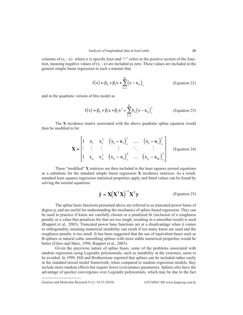
columns of (xi - k)+ where k is specific knot and “+” refers to the positive section of the func-

tion, meaning negative values of (xi - k) are included as zero. These values are included in the general simple linear regression in such a manner that

(Equation 22)

and in the quadratic version of this model as

(Equation 23)

The X incidence matrix associated with the above quadratic spline equation would then be modified to be:

(Equation 24)

These “modified” X matrices are then included in the least squares normal equations as a substitute for the standard simple linear regression X incidence matrices. As a result, standard least squares regression statistical properties apply and fitted values can be found by solving the normal equations:

(Equation 25)

The spline basis functions presented above are referred to as truncated power bases of degree p, and are useful for understanding the mechanics of spline-based regression. They can be used in practice if knots are carefully chosen or a penalized fit (inclusion of a roughness penalty or a value that penalizes fits that are too rough, resulting in a smoother result) is used (Ruppert et al., 2003). Truncated power base functions are at a disadvantage when it comes to orthogonality, meaning numerical instability can result if too many knots are used and the roughness penalty is too small. It has been suggested that the use of equivalent bases such as B-splines or natural cubic smoothing splines with more stable numerical properties would be better (Eilers and Marx, 1996; Ruppert et al., 2003).

Given the piecewise nature of spline bases, some of the problems associated with random regression using Legendre polynomials, such as instability at the extremes, seem to be avoided. In 1999, Hill and Brotherstone reported that splines can be included rather easily in the standard mixed model framework; when compared to random regression models, they include more random effects but require fewer (co)variance parameters. Splines also have the advantage of quicker convergence over Legendre polynomials, which may be due to the fact

30


S.E. Speidel et al.

that spline coefficients are more sparse than their polynomial counterparts (Misztal, 2006). One of the most important questions when using spline bases seems to be the number of knots needed to accurately describe the data, as well as where to place these knots. The use of too many knots will increase the complexity of the model, while the use of too few will reduce ac-curacy. Misztal (2006) suggests the following guidelines for choosing proper knot placement:

Choose knots in such a manner that they encompass the extremes observed in the data.Choose knots in a way that the correlations between knots are in the range of 0.6 to 0.8.These two suggestions will result in knots being placed close together around areas

that have the largest data density (i.e., birth weight, weaning weight, etc.), and will also result in a larger concentration of knots in areas where the data are changing more rapidly.

Until very recently, use of spline-based regression techniques by quantitative geneti-cists in the livestock industry had been almost non-existent. Spline basis functions have been used in the analysis of a number of traits, and as with the random regression and covariance function models, they were first used for the analysis of dairy cattle test day records. They have been incorporated into fixed regressions to model the lactation curve in the analysis of dairy cattle test day records (Druet et al., 2003), as well as the modeling of curves for esti-mated breeding values (EBV) (White et al., 1999).

The use of splines for the analysis of beef cattle data seems, so far, limited to the analysis of growth traits. Meyer (2005b) used quadratic B-splines to analyze Angus growth data from birth to 820 days of age, with knots at 0, 200, 400, 600, and 821 days of age. She found that the B-splines lend themselves well to the modeling of growth data, but they tend to be susceptible to irregularities in the distribution and sparseness of the data. Using simu-lated beef cattle growth data, Bohmanova et al. (2005) found that despite the fact that splines are simpler and have fewer parameters than Legendre polynomials, they are just as accurate (within 0.2%). A series of studies was conducted in 2005 and 2006 investigating the feasibility of using spline basis functions in random regression models that could be used for large-scale genetic evaluations (Iwaisaki et al., 2005; Robbins et al., 2005; Bertrand et al., 2006). In this set of studies, it was determined that random regression using spline bases is a feasible alterna-tive to random regression with Legendre polynomial bases and also to the more contemporary multivariate model.

CONCLUSIONS AND IMPLICATIONS FOR THE BEEF INDUSTRY

A topic of much discussion today among beef cattle geneticists is how to improve the accuracy of existing genetic evaluations. While much of this discussion is focused on the incorporation of DNA marker information into current genetic evaluation schemes (Schaeffer, 2006; Goddard and Hayes, 2007; Kachman, 2008), increasing the number of useable records would also add accuracy to a sire’s expected progeny differences. Current evaluation method-ology for growth uses a multivariate mixed model that treats weights recorded at successive ages as separate but genetically correlated traits. If the number of age groups for which ob-servations are measured is high, these problems can become very large and intractable rather quickly. As a result, the Beef Improvement Federation (BIF) recommends that weights be stan-dardized to a specified age (for example, weaning weights are typically adjusted to 205 days) or weights fall into specified age ranges (BIF recommended age range for weaning weight is 160 to 250 days) in order to be included in a genetic evaluation (BIF, 2002). Often manage-

31



ment decisions, such as early weaning strategies, lead to weights being recorded outside these recommended age ranges, and therefore render them unusable for genetic evaluation purposes. The use of random regression techniques can allow for the incorporation of observations taken at any number of ages. This is an advantage over conventional genetic evaluation methods, due to the fact that increasing the amount of useable data increases the accuracy of the genetic prediction, which can lead to an increased rate of genetic change (Williams et al., 2009).

Random regression methodology also has the potential to have a larger impact on the beef industry than just in the analysis of growth traits. It has the ability to identify cattle that require fewer days to reach their finish endpoint in the feedlot, a trait (group of traits) that has long been identified as being economically relevant (Lindholm and Stonaker, 1957; Golden et al., 2000). Besides the ability of random regression models to use data measured at a number of ages, the resulting EBV obtained from these models can be used for regression curves. Con-sequently, EBV could be calculated for any age or any number of days on feed. Kuehn (2000) presented an equation for the calculation of any customized EBV, where individual animals were estimated using a linear regression, as is shown below

EBV(age or weight) = b0 + b1*(desired age)

where b0 is the EBV for the intercept and b1 is the linear EBV for each individual sire. Fol-lowing Kuehn, Jublieu (2003) showed sufficient genetic variation existed for a selection tool expressed as days to finish weight. The EBVs obtained from a random regression model ap-parently have the potential to cause confusion, especially if higher order polynomials are used. Therefore, information packaging and information support of genetic evaluations that incorporate random regression approaches should be carefully considered.

Random regression techniques have the potential to greatly influence beef cattle ge-netic evaluation techniques. Their ability to incorporate recorded data from any number of ages into a single evaluation, by properly accounting for the changing covariance structure between observations, has the potential to have a large impact on genetic evaluation method-ology, with little to no change in current data recording schemes. As such, increases in the ac-curacy of an evaluation will be seen as these techniques become more widely used in national beef cattle evaluations.

REFERENCES

Beef Improvement Federation (BIF) (2002). Guidelines for Uniform Beef Improvement Programs. 8th edn. University of Georgia, Athens.

Bertrand JK, Misztal I, Robbins KR, Bohmanova J, et al. (2006). Implementation of Random Regression Models for Large Scale Evaluations for Growth in Beef Cattle. In: Proceedings of the 8th World Congress on Genetics Applied to Livestock Production, August 13-18, 2006, Belo Horizonte, MG, Brasil. CD-ROM Comm., Belo Horizonte, 03-04.

Bohmanova J, Misztal I and Bertrand JK (2005). Studies on multiple trait and random regression models for genetic evaluation of beef cattle for growth. J. Anim. Sci. 83: 62-67.

Carvalheira JG, Blake RW, Pollak EJ, Quaas RL, et al. (1998). Application of an autoregressive process to estimate genetic parameters and breeding values for daily milk yield in a tropical herd of Lucerna cattle and in United States Holstein herds. J. Dairy Sci. 81: 2738-2751.

Druet T, Jaffrezic F, Boichard D and Ducrocq V (2003). Modeling lactation curves and estimation of genetic parameters for first lactation test-day records of French Holstein cows. J. Dairy Sci. 86: 2480-2490.

Eilers PHC and Marx BD (1996). Flexible smoothing with B-splines and penalties. Statist. Sci. 11: 89-121.Foster JJ, Barkus E and Yavorsky C (2006). Understanding and Using Advanced Statistics: A practical guide for students.

(Equation 26)

32


S.E. Speidel et al.

1st edn. Sage Publications Ltd., London.Goddard ME and Hayes BJ (2007). Review article: Genomic selection. J. Anim. Breed. Genet. 124: 323-300.Golden BL, Garrick DJ, Newman S and Enns RM (2000). Economically Relevant Traits, a Framework for the Next

Generation of EPDs. In: Proceedings of the 32nd Research Symposium and Annual Meeting of the Beef Improvement Federation, Wichita, 2-13.

Harville DA (1979). Recursive Estimation Using Mixed Linear Model with Autoregressive Random Effects. In: Variance Components and Animal Breeding, Proceedings of the Conference in Honor of C.R. Henderson, Cornell University, Ithaca, 157-179.

Henderson CR Jr (1982). Analysis of covariance in the mixed model: higher-level, nonhomogeneous, and random regressions. Biometrics 38: 623-640.

Henderson CR and Quaas RL (1976). Multiple trait evaluation using relatives’ records. J. Anim. Sci. 43: 1188-1197.Hill WG and Brotherstone S (1999). Advances in Methodology for Utilizing Sequential Records. In: Metabolic stress in

dairy cows (Oldham JD, Simm G, Groen AF, Nielsen BL, et al., eds.). British Society of Animal Science Occasional Publication, No. 24, 55-61.

Interbull (2000). National Genetic Evaluation Programmes for Dairy Production Traits Practised in Interbull Member Countries 1999-2000. Department of Animal Breeding and Genetics, Uppsala, Bulletin 24.

Iwaisaki H, Tsuruta S, Misztal I and Bertrand JK (2005). Genetic parameters estimated with multitrait and linear spline-random regression models using Gelbvieh early growth data. J. Anim. Sci. 83: 757-763.

Jamrozik J, Kistemaker GJ, Dekkers JC and Schaeffer LR (1997a). Comparison of possible covariates for use in a random regression model for analyses of test day yields. J. Dairy Sci. 80: 2550-2556.

Jamrozik J, Schaeffer LR and Dekkers JC (1997b). Genetic evaluation of dairy cattle using test day yields and random regression model. J. Dairy Sci. 80: 1217-1226.

Jennrich RI and Schluchter MD (1986). Unbalanced repeated-measures models with structured covariance matrices. Biometrics 42: 805-820.

Jublieu JS (2003). The Use of Random Regression Models to Predict Days to Finish in Beef Cattle. Master’s thesis, Colorado State University, Fort Collins.

Kachman SD (2008). Incorporation of Marker Scores into National Genetic Evaluation. In: Proceedings of the 9th Genetic Prediction Workshop Beef Improvement Federation, Kansas City, 92-98.

Kachman SD and Everett RW (1993). A multiplicative mixed model when the variances are heterogeneous. J. Dairy Sci. 76: 859-867.

Kirkpatrick M and Heckman N (1989). A quantitative genetic model for growth, shape, reaction norms, and other infinite-dimensional characters. J. Math. Biol. 27: 429-450.

Kirkpatrick M, Lofsvold D and Bulmer M (1990). Analysis of the inheritance, selection and evolution of growth trajectories. Genetics 124: 979-993.

Kirkpatrick M, Hill WG and Thompson R (1994). Estimating the covariance structure of traits during growth and ageing, illustrated with lactation in dairy cattle. Genet. Res. 64: 57-69.

Koots KR, Gibson JP and Wilton JW (1994). Analyses of published genetic parameter estimates for beef production traits. 2. Phenotypic and genetic correlations. Anim. Breed. Abstr. 62: 825-853.

Kuehn LA (2000). Parameterization of Random Regression Models for Beef Cattle Data Sets. Master’s thesis, Colorado State University, Fort Collins.

Laird NM and Ware JH (1982). Random-effects models for longitudinal data. Biometrics 38: 963-974.Lindholm HB and Stonaker HH (1957). Economic importance of traits and selection indexes for beef cattle. J. Anim. Sci.

16: 998-1006.López-Romero P, Rekaya R and Carabaño MJ (2003). Assessment of homogeneity vs. heterogeneity of residual variance

in random regression test-day models in a Bayesian analysis. J. Dairy Sci. 86: 3374-3385.López-Romero P, Rekaya R and Carabaño MJ (2004). Bayesian comparison of test-day models under different assumptions

of heterogeneity for the residual variance: the change point technique versus arbitrary intervals. J. Anim. Breed. Genet. 121: 14-25.

Meyer K (2004). Scope for a random regression model in genetic evaluation of beef cattle for growth. Livest. Prod. Sci. 86: 69-83.

Meyer K (2005a). Advances in methodology for random regression analyses. Aust. J. Exp. Agric. 45: 847-858.Meyer K (2005b). Random regression analyses using B-splines to model growth of Australian Angus cattle. Genet. Sel.

Evol. 37: 473-500.Meyer K and Hill WG (1997). Estimation of genetic and phenotypic covariance functions for longitudinal or ‘repeated’

records by restricted maximum likelihood. Livest. Prod. Sci. 47: 185-200.Meyer K and Kirkpatrick M (2005). Up hill, down dale: quantitative genetics of curvaceous traits. Philos. Trans. R. Soc.

33



Lond B Biol. Sci. 360: 1443-1455.Misztal I (2006). Properties of random regression models using linear splines. J. Anim. Breed. Genet. 123: 74-80.Mrode RA (2005). Linear Models for the Prediction of Animal Breeding Values. 2nd edn. CABI Publishing Company,

Cambridge.Olori VE, Hill WG and Brotherstone S (1999). The Structure of the Residual Error Variance of Test Day Milk Yield

in Random Regression Models. In: Proceeding of Computational Cattle Breeding Workshop, March 18-20, 1999, Interbull Bulletin, Tuusula, 103-108.

Pander BL, Hill WG and Thompson R (1992). Genetic parameters of test day records of British Holstein-Friesian heifers. Anim. Prod. 55: 11-21.

Ptak E and Schaeffer LR (1993). Use of test day yields for genetic evaluation of dairy sires and cows. Livest. Prod. Sci. 34: 23-34.

Rekaya R, Carabano MJ and Toro MA (2000). Assessment of heterogeneity of residual variances using change point techniques. Genet. Sel. Evol. 32: 383-394.

Robbins KR, Misztal I and Bertrand JK (2005). A practical longitudinal model for evaluating growth in Gelbvieh cattle. J. Anim. Sci. 83: 29-33.

Robert-Granié C, Maza E, Rupp R and Foulley JL (2002). Use of fractional polynomial for modelling somatic cell scores in dairy cattle. In: Proceedings of the 7th World Congress on Genetics Applied to Livestock Production, August 19-23, Communication No. 16-05, Montpellier, CD-ROM.

Ruppert D, Wand MP and Carroll RJ (2003). Cambridge Series in Statistical and Probabilistic Mathematics: Semiparametric Regression. Cambridge University Press, New York.

Schaeffer LR (2003). Random regression models. ANSC637 Course Notes - Quantitative genetics and animal models. Available at [http://www.aps.uoguelph.ca/%7Elrs/ABModels/NOTES/RRM14a.pdf]. Accessed January 8, 2009.

Schaeffer LR (2004). Application of random regression models in animal breeding. Livest. Prod. Sci. 86: 35-45.Schaeffer LR (2006). Strategy for applying genome-wide selection in dairy cattle. J. Anim. Breed. Genet. 123: 218-223.Schaeffer LR and Jamrozik J (1996). Multiple-trait prediction of lactation yields for dairy cows. J. Dairy Sci. 79: 2044-2055.Schaeffer LR and Jamrozik J (2008). Random regression models: a longitudinal perspective. J. Anim. Breed. Genet. 125:

145-146.Schaeffer LR, Swalve HH and Dekkers JCM (1994). Random Regressions in Animal Models for Test-day Production in Dairy

Cattle. In: Proceedings of the 5th World Congress of Genetic and Applied Livestock Production, Guelph, 433-446.Torres RAA Jr and Quaas RL (2001). Determination of covariance functions for lactation traits on dairy cattle using

random-coefficient regressions on B-splines. J. Anim. Sci. (Suppl 1) 79: 112 (Abstract).White IM, Thompson R and Brotherstone S (1999). Genetic and environmental smoothing of lactation curves with cubic

splines. J. Dairy Sci. 82: 632-638.Wiggans GR and Goddard ME (1996). A computationally feasible test day model with separate first and later lactation

genetic effects. Proc. N. Z. Soc. Anim. Prod. 56: 19-21.Wiggans GR and Goddard ME (1997). A computationally feasible test day model for genetic evaluation of yield traits in

the United States. J. Dairy Sci. 80: 1795-1800.Williams JL, Garrick DJ and Speidel SE (2009). Reducing bias in maintenance energy expected progeny difference by

accounting for selection on weaning and yearling weights. J. Anim. Sci. 87: 1628-1637.Wold S (1974). Spline functions in data analysis. Technometrics 16: 1-11.Wright S (1922). Coefficients of inbreeding and relationship. Am. Nat. 56: 330-338.

Review Genetic analysis of longitudinal data in beef ... · Review Genetic analysis of longitudinal data in beef ... Department of Animal Sciences, Colorado State University, Fort

Documents