THESIS RESOURCE ALLOCATION FOR WILDLAND FIRE SUPPRESSION PLANNING USING A STOCHASTIC PROGRAM Submitted by Alex Taylor Masarie Department of Forest and Rangeland Stewardship In partial fulfillment of the requirements For the Degree of Master of Science Colorado State University Fort Collins, Colorado Fall 2011 Master’s committee: Advisor: Douglas Rideout Michael Bevers Michael Kirby

Welcome message from author
This document is posted to help you gain knowledge. Please leave a comment to let me know what you think about it! Share it to your friends and learn new things together.
Transcript

THESIS
RESOURCE ALLOCATION FOR WILDLAND FIRE SUPPRESSION PLANNING
USING A STOCHASTIC PROGRAM
Submitted by
Alex Taylor Masarie
Department of Forest and Rangeland Stewardship
In partial fulfillment of the requirements
For the Degree of Master of Science
Colorado State University
Fort Collins, Colorado
Fall 2011
Master’s committee:
Advisor: Douglas Rideout
Michael Bevers Michael Kirby
ii
ABSTRACT
RESOURCE ALLOCATION FOR WILDLAND FIRE SUPPRESSION PLANNING
USING A STOCHASTIC PROGRAM
Resource allocation for wildland fire suppression problems, referred to here as
Fire-S problems, have been studied for over a century. Not only have the many variants
of the base Fire-S problem made it such a durable one to study, but advances in
suppression technology and our ever-expanding knowledge of and experience with
wildland fire behavior have required almost constant reformulations that introduce new
techniques. Lately, there has been a strong push towards randomized or stochastic
treatments because of their appeal to fire managers as planning tools. A multistage
stochastic program with variable recourse is proposed and explored in this paper as an
answer to a single-fire planning version of the Fire-S problem. The Fire-S stochastic
program is discretized for implementation according to scenario trees, which this paper
supports as a highly useful tool in the stochastic context. Our Fire-S model has a high
level of complexity and is parameterized with a complicated hierarchical cluster analysis
of historical weather data. The cluster analysis has some incredibly interesting features
and stands alone as an interesting technique apart from its application as a
parameterization tool in this paper. We critique the planning model in terms of its
complexity and options for an operational version are discussed. Although we assume no

iii
interaction between fire spread and suppression resources, the possibility of incorporating
such an interaction to move towards an operational, stochastic model is outlined. A
suppression budget analysis is performed and the familiar ``production function'' fire
suppression curve is created, which strongly indicates the Fire-S model performs in
accordance with fire economic theory as well as its deterministic counterparts. Overall,
this exploratory study demonstrates a promising future for the existence of tractable
stochastic solutions to all variants of Fire-S problems.

iv
ACKNOWLEDGEMENTS
I would like to acknowledge the invaluable help of my advisors on this project.
Thanks to Dr. Mike Bevers from the Forest Service for everything from guiding the
fundamentals of the mathematics to discussions of obscure details. Thanks to Dr. Douglas
Rideout from the Forest, Rangeland, and Watershed Stewardship Department for helping
the overall focus of the project, guiding the economic context, and keeping up with math
he does not work with on a day-to-day basis. Thanks to Dr. Michael Kirby from the
Colorado State University Math Department for a great class on linear optimization and
discussions about fire science problems. I would also like to thank the people that helped
track down or teach me the tools, without which the Fire-S model cannot run. Thanks to
Peter Barry for two great fire science classes in which I learned all about fire behavior
simulation and the tools available to make it realistic. Thanks to Mark Finney for Farsite.
Thanks to Stu Brittain for making the Farsite DLL available online. Thanks to Angie
Hinker and the staff at the Northern Great Plains Interagency Dispatch Center in Rapid
City, South Dakota for spending such a big chunk of time teaching me the ins and outs of
dispatch.
v
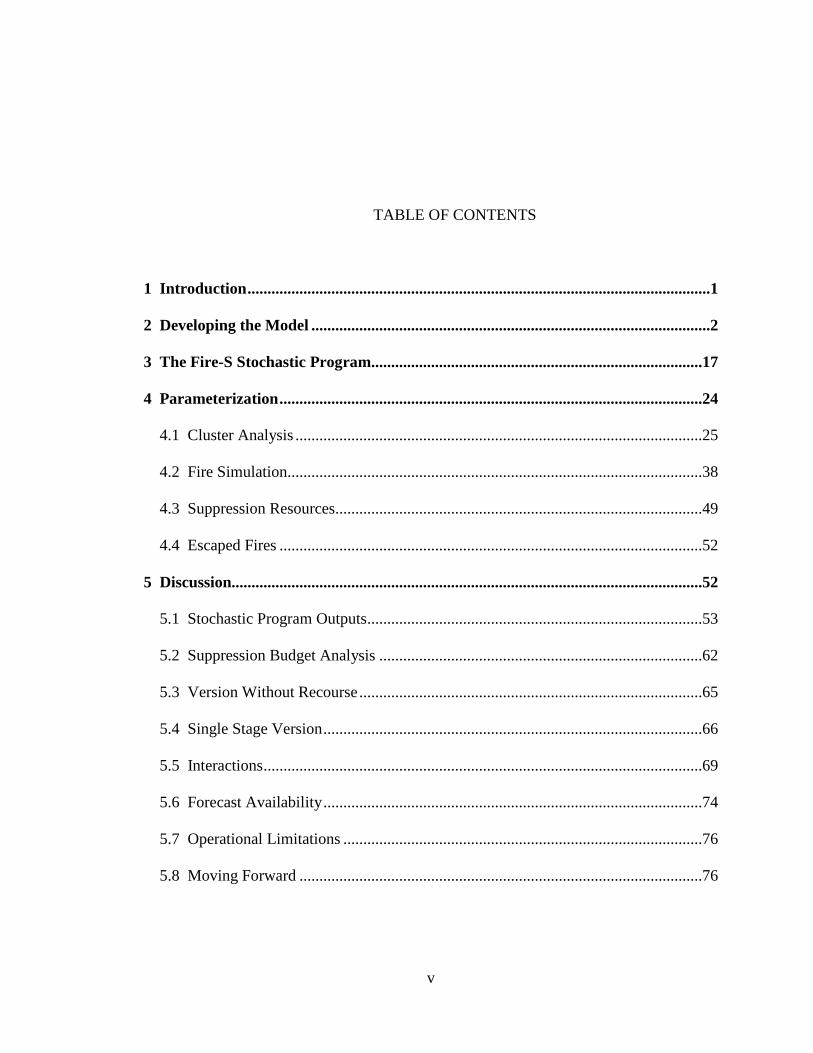
TABLE OF CONTENTS
1 Introduction ....................................................................................................................1
2 Developing the Model ....................................................................................................2
3 The Fire-S Stochastic Program...................................................................................17
4 Parameterization ..........................................................................................................24
4.1 Cluster Analysis ......................................................................................................25
4.2 Fire Simulation........................................................................................................38
4.3 Suppression Resources............................................................................................49
4.4 Escaped Fires ..........................................................................................................52
5 Discussion......................................................................................................................52
5.1 Stochastic Program Outputs ....................................................................................53
5.2 Suppression Budget Analysis .................................................................................62
5.3 Version Without Recourse ......................................................................................65
5.4 Single Stage Version ...............................................................................................66
5.5 Interactions ..............................................................................................................69
5.6 Forecast Availability ...............................................................................................74
5.7 Operational Limitations ..........................................................................................76
5.8 Moving Forward .....................................................................................................76

1
1 Introduction Much of the fire business on a given district involves initial attack on containable
fires. Fire economists and fire managers have long studied the initial attack resource
allocation for fire suppression problem. Fire management models that support the Fire
Program Analysis (FPA) represent the vast work done on this subject. Models described
by Donovan and Rideout in [5] as well as Kirsch and Rideout in [9] are deterministic
solutions to the problem. Others have studied initial attack in a probabilistic (or
stochastic) framework. A prime example of such stochastic modeling is the California
Fire Economics Simulator (CFES). Underlying CFES is the random simulation model
presented by Fried, Gilless, and Spero in [8].
Stochastic models can be more complicated than their deterministic counterparts,
but also provide significant advantages as realistic planning tools. We present a stochastic
programming model that solves a single fire version of the allocation for suppression
problem, which is referred to as the Fire-S model. We propose a four-stage stochastic
program with variable recourse and explain the underlying mathematics. Section 2
develops the model from a simple example building to the actual model presented in
Section 3. Such a stochastic program allows us to (a) capture the dynamic aspect of fire
suppression in the four stages and (b) reconcile the reality that decisions made over time
demonstrate a hierarchical dependence using recourse. Just like any math programming
model, our stochastic program has decision variables and parameters. The decision
variables represent resource allocation choices. The parameters represent a fire manager's
resource set and the fire behavior he or she encounters. We simulate fire behavior
parameters by performing a cluster analysis of historical weather data, which produces

2
representative weather scenarios to use in the Fire Area Simulator (Farsite) software
package. We describe the parameterization steps in Section 4, which consists of weather
in Section 4.1, fire simulation in Section 4.2, suppression resources in Section 4.3, and
escaped fires in Section 4.4. Although the parameterization process is spatially explicit,
the stochastic program itself is not. The program does not, for instance, account for the
interaction between fire growth and suppression, which we explore in Sections 5.5 and
5.7. As such, our model is most readily interpreted as a fire planning model instead of an
operational model. Section 5.2 shows how the Fire-S model supports suppression budget
analysis. We use the suppression budget analysis to search for advantages for the model's
complexity in Sections 5.3 and 5.4. This exploration concludes with a discussion of
promising avenues of further research in Section 5.8.
2 Developing the Model
Figure 1: Our single-fire time line.
Figure 1 shows the dynamic aspect of our version of the single-fire allocation for
suppression problem. First, notice there are four interdependent stages. For clarity, we

3
assume each stage lasts twelve hours and so the scope of the model is two days, although
this assumption is not necessary. An initial smoke report indicates a fire exists on the
landscape during Stage 1, which, assuming twelve-hour stage lengths, means the morning
of Day 1. Figure 1 also gives some possible terms associated with the fire from initial
attack to possible containment. These descriptors are merely a demonstration of one
possible scenario; many factors influence fire suppression. Also notice Stage 4 is marked
as the ``escape stage.'' This means the fire has escaped containment in the scope of
model. It need not be assumed an extreme fire, just that uncertainty in fire behavior
factors such as weather and fuels is quite high for a fire manager applying these
techniques at a stage 1 smoke report. We discuss implementing a rolling planning horizon
to address this issue later on.
Although the stochastic program follows these stages, the user applies the model
just once at the start of Stage 1. All of the user's information about subsequent stages is
probabilistic and therefore uncertain. Recourse operates in this program by assuming
various possible scenarios occur. Thus, once a scenario is adopted or realized (with its
associated probability) the uncertainty is eliminated and a decision can be made. The
most basic example of recourse involves containment. Suppose a fire manager has
allocated enough resources to contain the fire in Stage 2. Stage 3's recourse decisions
must reflect the fact that the fire is contained under the current scenario and perhaps
allocate a mop-up crew or do nothing at all.
Scenarios are the key, underlying tool that we use to parameterize the stochastic
program and make the model realistic. One of the benefits of a probabilistic approach is
that we can work with two basic concepts of fire management:

4
1. A fire manager CANNOT exactly predict fire behavior with complete
certainty over time,
2. A fire manager CAN incorporate expert knowledge and/or fire behavior
software to characterize some likely and unlikely fire behaviors.
Thus, a fire manager is a highly capable predictor of fire behavior and can use his
or her numerous, scientific tools to construct a collection of possible fire behavior
scenarios, which we call a scenario tree.
We will start with a small-scale example of such a scenario tree and proceed to
build towards the stochastic program as a whole. Suppose a smoke report indicates an
ignition in a given fire management zone. The fire manager uses the ignition's spatial
location to obtain detailed fuels and topographical information. Given the ignition's
temporal location (time of day, season, etc...) the fire manager also obtains current fire
weather information and forecasts. Say, in this simple example, there are two common
weather patterns associated with the passage of summertime cold fronts through the area.
In reality, the fire manager would have fairly accurate predictions about when the front
will pass, but, for the sake of this example, let us assume each of these two weather
scenarios (pre-frontal and post-frontal) has a 50% chance of occuring. Furthermore, the
fire manager does not know when, during the two day scope of this model, fronts will
pass. Using pre-frontal and post-frontal weather data, the fire manager runs Farsite and
determines fire behavior for all possible front arrival times during each of the four stages.

5
Figure 2: A two-branch scenario tree example.
Figure 2 shows the resulting sixteen fire behavior scenarios. Right now, at the
time of the smoke report, the fire manager does not know which branch will best match
the actual fire behavior (concept 1), but he or she is confident that Figure 2 represents a
clear picture of possible fire behaviors (concept 2) because it is based on the best
available weather and a scientifically sound simulation software package.
The scenario tree in Figure 2 is a crucial part of the model so we will explore it
thoroughly. The solid lines connecting the diagram together are called branches.

6
Branches initiate and terminate at nodes. In terms of the time-line in Figure 1, the
branches represent periods of time during a stage and the nodes represent transitions
between stages. Decisions are made at nodes and their actions carried out during
branches. At any given Stage 1, 2, or 3 node there is one branch that represents moderate
fire behavior and another that represents severe fire behavior. These are associated with
the fire manager's pre-frontal and post-frontal Farsite simulations. A scenario tree
diagram makes the hierarchical nature of the four-stage problem easy to follow. The fire
manager can literally trace each of the sixteen fire behavior scenarios by starting at the
leftmost node and finishing at each of the rightmost nodes. For example, the Farsite
simulation that represents moderate fire behavior for Stages 1, 2, and 3 and more severe
fire behavior for Stage 4 is found by tracing the top branch at the first three nodes and
then the bottom branch the final, stage 4 node. To represent this scenario we use an
ordered pair (1,1,1,2) . This way, each scenario has a unique representation ),,,( 4321 kkkk
where ,,, 321 kkk and 4k each take the value 1 or 2 . We say scenario (1,1,1,2) has parent
nodes (1,1,1) , (1,1) , and (1) . In general, we use the notation ⟩⟨ tk to represent an
ordered pair at Stage t ; so )(= 11 kk ⟩⟨ , ),(= 212 kkk ⟩⟨ , ),,(= 3213 kkkk ⟩⟨ , and
),,,(= 43214 kkkkk ⟩⟨ . Thus, in the equations to follow )(⋅ and ⟨⋅⟩ serve as visual
indicators the associated variables come from a scenario tree like Figure 2 and are
probabilistic.
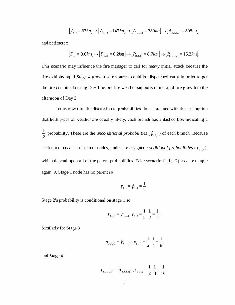
The boxes in Figure 2 show cumulative area ( ⟩⟨ tkA ) and perimeter ( ⟩⟨ tkP )
estimates at each node. Under scenario (1,1,1,2) the fire manager will encounter a fire
that grows in area as follows:
7
[ ] [ ] [ ] [ ]haAhaAhaAhaA 808=280=147=37= (1,1,1,2)(1,1,1)(1,1)(1) →→→
and perimeter:
[ ] [ ] [ ] [ ].15.2=8.7=6.2=3.0= (1,1,1,2)(1,1,1)(1,1)(1) kmPkmPkmPkmP →→→
This scenario may influence the fire manager to call for heavy initial attack because the
fire exhibits rapid Stage 4 growth so resources could be dispatched early in order to get
the fire contained during Day 1 before fire weather supports more rapid fire growth in the
afternoon of Day 2.
Let us now turn the discussion to probabilities. In accordance with the assumption
that both types of weather are equally likely, each branch has a dashed box indicating a
21 probability. These are the unconditional probabilities ( ⟩⟨ tkp ) of each branch. Because
each node has a set of parent nodes, nodes are assigned conditional probabilities ( ⟩⟨ tkp ),
which depend upon all of the parent probabilities. Take scenario (1,1,1,2) as an example
again. A Stage 1 node has no parent so
.21=ˆ= (1)(1) pp
Stage 2's probability is conditional on stage 1 so
.41=
21
21=ˆ= (1)(1,1)(1,1) ⋅⋅ ppp
Similarly for Stage 3
81=
41
21=ˆ= (1,1)(1,1,1)(1,1,1) ⋅⋅ ppp
and Stage 4
.161=
81
21=ˆ= (1,1,1)(1,1,1,2)(1,1,1,2) ⋅⋅ ppp

8
These conditional probabilities are shown in dashed circles on Figure 2. For this simple
example, conditional and unconditional probabilities are uniform, but this need not be the
case. When a fire manager is using expert knowledge to construct a scenario tree, he or
she will come up with a spectrum ranging from highly likely to highly unlikely fire
behavior scenarios to account for. Section 4 shows how we create a scenario tree with
non-uniform probabilities. This simple example demonstrates two important properties
about the conditional probabilities:
{ 1<0 ≤⟩∀⟨ ⟩⟨ tkt pk (2.1)
.1=
∀ ⟩⟨⟩⟨
∑ tk
tkpt (2.2)
Equation (2.1) is a familiar, general property of fractional probabilities that constrains
⟩⟨ tkp to be from 0 % to 100 %. The property in (2.2) means if we sum across each stage
(vertically in Figure 2), we get 100% probability. If we sum scenario probabilities for
Stage 3, for instance, Equation (2.2) becomes
1.=81==
2
1=3
2
1=2
2
1=1
)3,2,1(
3213
3
∑∑∑∑∑∑∑ ⟩⟨⟩⟨ kkk
kkkkkk
kk
pp
Thus, (2.2) ensures that some scenario occurs; in the Fire-S model, some fire behavior
occurs with 100% probability.
With this understanding of scenario trees, the next step is to explain how decision-
making operates in this framework. Figure 2 is a probabilistic description of fire
behavior. A fire manager wants to take this information and make resource allocation
decisions that are cost effective and achieve some set of management goals. We follow
9
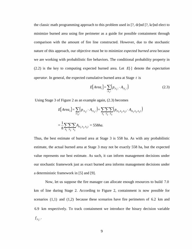
the classic math programming approach to this problem used in [?, dr]nd [?, kr]nd elect to
minimize burned area using fire perimeter as a guide for possible containment through
comparison with the amount of fire line constructed. However, due to the stochastic
nature of this approach, our objective must be to minimize expected burned area because
we are working with probabilistic fire behaviors. The conditional probability property in
(2.2) is the key to computing expected burned area. Let ][⋅E denote the expectation
operator. In general, the expected cumulative burned area at Stage t is
[ ] ( ).= ⟩⟨⟩⟨⟩⟨
⋅∑ tktk
tkt ApAreaE (2.3)
Using Stage 3 of Figure 2 as an example again, (2.3) becomes
[ ] ( ) ( ))3,2,1()3,2,1(
32133
3
3 == kkkkkkkkk
kkk
ApApAreaE ⋅⋅ ∑∑∑∑ ⟩⟨⟩⟨⟩⟨
.558=81= )3,2,1(
321
haA kkkkkk∑∑∑
Thus, the best estimate of burned area at Stage 3 is 558 ha. As with any probabilistic
estimate, the actual burned area at Stage 3 may not be exactly 558 ha, but the expected
value represents our best estimate. As such, it can inform management decisions under
our stochastic framework just as exact burned area informs management decisions under
a deterministic framework in [5] and [9].
Now, let us suppose the fire manager can allocate enough resources to build 7.0
km of line during Stage 2. According to Figure 2, containment is now possible for
scenarios (1,1) and (1,2) because these scenarios have fire perimeters of 6.2 km and
6.9 km respectively. To track containment we introduce the binary decision variable
⟩⟨ tkf .

10
Figure 3: One possible containment scenario for Figure 2.
Figure 3 shows the values this decision variable takes when 7.0 km of line can be
built and is called a containment scenario. Remember that we are performing this
calculation for Stage 3 so ⟩⟨ 2kf and ⟩⟨ 3kf are both relevant. We will formally define ⟩⟨ tkf
in Section 3, we emphasize that it indicates the stage during which containment is
declared. If 0=⟩⟨ tkf , then the fire may be burning uncontained or have been previously
declared contained. This subtlety is important when we compute expected burned area for
Figure 3's containment scenario. Before we do so however, notice this definition of ⟩⟨ tkf
supports recourse in the model. If a fire scenario is declared to be contained during Stage
2, then we assume it is contained throughout Stages 3 and 4.
The expression in (2.3) gives expected burned area for a single stage, but we now
have two interdependent stages so the expectation operators must be nested as follows:
]].[[=][ 32 AreaEAreaEAreaE + (2.4)
The reader may ask why Equation 2.4 does not take the form ][][ 32 AreaEAreaE + ?
Formulating (2.4) as shown, the expected burned area in Stage 2 can depend on the
expected burned area in Stage 3, which captures recourse in the fire manager's decision
making. A recourse decision is a decision made after some uncertainty in the problem
has been accounted for. We account for uncertainty each stage by introducing more
branches and conditional probabilities into the scenario tree. Stage 2 and Stage 3 are not

11
independent as ][][ 32 AreaEAreaE + would suggest. Burned area in Stage 2, may well
depend on the expected burned area in Stage 3, so the overall expected burned area must
be nested as in (2.4).
These computations can be convoluted so we move through this one in detail. In
terms of the scenario tree in Figure 2,
( )].[=][ )3,2,1()3,2,1()3,2,1()3,2,1(
)2,1()2,1()2,1()2,1(
kkkkkkkkkkkk
kkkkkkkk
fApfApAreaE ∑∑ + (2.5)
The expression in (2.5) is a two stage version of (2.3). It goes further than (2.3) because
it incorporates the nesting of expectation operators in (2.4) and the decision variable
⟩⟨ tkf . Area will be added to the total if and only if 1=⟩⟨ tkf . We have dropped the ⟨⋅⟩
notation so as not to double count in the sum. Expanding the summation in (2.5) we see
(1,1,2)(1,1,2)(1,1,2)(1,1,1)(1,1,1)(1,1,1)(1,1)(1,1)(1,1)=][ fApfApfApAreaE ++
(1,2,2)(1,2,2)(1,2,2)(1,2,1)(1,2,1)(1,2,1)(1,2)(1,2)(1,2) fApfApfAp +++
(2,1,2)(2,1,2)(2,1,2)(2,1,1)(2,1,1)(2,1,1)(2,1)(2,1)(2,1) fApfApfAp +++
.(2,2,2)(2,2,2)(2,2,2)(2,2,1)(2,2,1)(2,2,1)(2,2)(2,2)(2,2) fApfApfAp +++
According to Figure 3 half of these terms are zero so
(2,1,2)(2,1,2)(2,1,1)(2,1,1)(1,2)(1,2)(1,1)(1,1)=][ ApApApApAreaE +++
,(2,2,2)(2,2,2)(2,2,1)(2,2,1) ApAp ++
which we can calculate with corresponding values from Figure 2 to give
)(78781)(492
81)(203
41)(147
41=][ hahahahaAreaE +++
.466.875=)(99981)(757
81 hahaha ++

12
If the fire manager elects to deploy resources and contain the fire under scenarios (1,1)
and (1,2) , then the expected burned area will be about 467 ha, which is 91 ha less than
the expected Stage 3 burn area without any suppression activity (558 ha). The Fire-S
model is a four stage model so we will be adding an additional stage to these
computations when we discuss the full version of the Fire-S stochastic program in
Section 3.
As mentioned, containment involves deployment of resources. Not only do these
resources cost money, but they also come from a scarce set and have realistic constraints
such as travel time and line production rates. We will continue to build this example by
discussing the resource set shown in Table 1.
Table 1 r Description FC ($) VC ($/hr) Production (chains/hr) 1 Dozer 11,600 900 30 2 Type I Hand Crew 2,050 250 9 3 Type II Hand Crew A 1,000 100 6 4 Type II Hand Crew B 1,200 100 7 5 Engine 1 8,200 500 16 6 Engine 2 7,600 550 16 7 Engine 3 4,500 300 12
Table 1: Example resource set.
To build at least 7.0 kilometers of line during Stage 2, the fire manager has
various alternatives. Three of these alternatives are shown with the costs they incur in
Table 2. Remember that Stage 2 is twelve hours is long so we have incorporated the
reasonable assumption of an eight-hour line producing period in these calculations and
the full stochastic program. Variable costs will be incurred for each hour the resource is
active.

13
Table 2 Alternative Resource Package Stage 2 Production (km) Cost ($)
A 1, 2, and 3 7.2 29,650 B 5, 6, and 7 7.1 36,500 C 2, 4, 5, and 7 7.0 29,750
Table 2: Alternative resource packages to build at least 7.0 km of line.
The fire manager may deem Alternative A (a dozer and two hand crews) in Table
2 optimal because it is the cheapest way to achieve the line-building requirements.
Alternative B deploys three engines, which is costly and probably unnecessary.
Alternative C is also attractive because the deployment package calls for two hand crews
and two engines, which may be more practical for a wild land urban interface (WUI), at
only a slightly higher cost.
While cost minimization is a common objective for fire suppression, we choose to
incorporate cost as a constraint, which affords us the natural interpretation of expenditure
under a fixed budget. Say the fire manager has a budget goal of $44,000 for this fire. Let
⟩⟨ tkrx , be a binary decision variable (like ⟩⟨ tkf ) that tracks resource deployment. If
1=, ⟩⟨ tkrx , then resource r is in transit to or active on the fire during Stage t under
scenario ⟩⟨ tk . If 0=, ⟩⟨ tkrx , then it is not. Each resource r has a set of associated
parameters: the variable cost of actively building line during Stage t ( trVC , ), the fixed
cost of deployment ( rFC ), and the line production rate under scenario ⟩⟨ tk ( ⟩⟨ tkrL , ). All
three parameters can be read from Table 1 for this example. But, when does a resource
actually start to build line? We assume 1=, ⟩⟨ tkrx means the resource is ordered during
Stage t and will start producing line at the start of Stage 1+t . Any preparation and travel
time is rolled into the resource ordering stage. For example, if the fire manager wants

14
Engine 1 ( 5=r ) to contribute fire line during the Stage 2 scenario (1,1)=2⟩⟨k , the order
will be placed during Stage 1 by specifying 1=(1)5,x , perhaps just after the initial smoke
report. The fire manager must budget for the fixed cost of Engine 1, $8,200=5FC , and
the variable cost of operation during the twelve hours of Stage 2,
$6,000,=12$500=5,2 hrshr
VC ⋅
when he or she orders it. Thus, alternatives A, B, and C must satisfy the following budget
constraint
[ ]( ) $44,000,,2(1),1=
≤+∑ rrr
R
rFCVCx
where R is the size of the resource set, in our case 7=R . According to Table 2, all three
alternatives satisfy the budget constraint. Of the three, Alternative A is the most cost
effective choice to achieve containment under scenarios (1,1) and (1,2) . We can use
Alternative A to demonstrate how our containment constraints function in the stochastic
program. We follow the classic approach, which means in order to contain a fire, line
production must exceed fire perimeter. For scenario (1,1) the containment constraint is
( ) .(1,1)(1,1)(1,1),(1),1=
PfLx rrr
≥∑
We permit containment ( 1=(1,1)f ) if and only if line production exceeds fire perimeter.
Choosing Alternative A permits containment for scenarios (1,1) and (1,2) because we
see the total Stage 2 line production from Table 2 is 7.2 km, which exceeds fire
perimeter 6.2=(1,1)P km. We do not permit containment for scenario (2,1) nor (2,2)
because in each case fire perimeter exceeds line production.

15
Even though 0== (2,2)(2,1) ff when Alternative A is deployed, let us illustrate a
multistage containment by assuming the fire manager will elect Alternative A for both
Stage 1 branches: (1) and (2) . First, let us examine whether or not Alternative A
satisfies the budget. Table 2 shows that Alternative A costs $29,650. With a budget of
$44,000 that leaves $14,350 to use for the Stage 3 suppression effort. This may not seem
like enough, but remember the fixed costs have already been paid, so only variable costs
are incurred for Stage 3. During the twelve-hour Stage 3 the dozer and hand crews incur
$15,000 in variable costs. This does exceed the budget so Alternative A cannot be used
to achieve a multistage containment. Fortunately, we can turn to Alternative C, satisfy the
budget, and still achieve the Stage 2 containment we desire. But, does Alternative C
permit any Stage 3 containment? Variable costs for Alternative C are low enough that
$43,550 covers the Stage 2 and 3 suppression costs. Alternative C is permitted under the
budget constraint level of $44,000. Suppose the engines and crews in Alternative C
perform strategic attack and construct their 7.0 km of line along the fire's flank during
Stage 2 for scenario (2,1) . Since 8.1=(2,1)P km, this is not enough line for containment,
but if they continue to produce line (at the same rates), they will construct 14.0 km by the
end of Stage 3. Since 10.0=(2,1,1)P km, this is enough line to contain the fire during Stage
3 under this scenario. Therefore, we say Alternative C can perform a multistage
containment for scenario (2,1,1) .
If we consult Figure 2, we see 14.0 km is not enough fire line to contain the fires
in scenarios (2,1,2) , (2,2,1) , or (2,2,2) . This means the new containment scenario
differs from that of Figure 3 because

16
0=== (2,2,2)(2,2,1)(2,1,2) fff
and the fire will continue to grow into Stage 4 for these scenarios. The fire manager has
exhausted the budget so the remaining scenarios represent escaped fires. Escaped fires
may not necessarily be synonymous with extreme fires, but these fire scenarios extend
beyond the time frame that the fire manager has decided is reasonable for fire weather
and behavior predictions (Figure 1). How do we account for the six escaped fires in
Figure 2? In terms of the Fire-S model, the fire manager was not able to contain the fire
under these behavior scenarios because fire spread was too great; so he or she expects
each one to transition to a large fire. In order to get an expected burned area like (2.3) we
must provide an estimate for a large fire area to account for escape scenarios. Suppose the
fire manager consults a Fire Family Plus database and comes up with a large fire area
estimate based on historical records of 7,814=ˆLFA ha. If we track escape scenarios
using the binary decision variable ⟩⟨ 4kesc (equals 1 when a fire escapes), then the
expected burned area is
)3,2,1()3,2,1()3,2,1(
3
)2,1()2,1()2,1(
21
[([=][ kkkkkkkkkk
kkkkkkkk
fApfApAreaE ∑∑∑ +
( )])].ˆ)4,3,2,1()4,3,2,1(
4
kkkkLFkkkkk
escAp∑+ (2.6)
The expression in (2.6) is a four stage version of (2.5) that also accounts for escaped fire
scenarios. For the example scenario tree in Figure 2 we denote the six escape scenarios
with
1====== (2,2,2,1)(2,2,2,1)(2,2,1,2)(2,2,1,1)(2,1,2,2)(2,1,2,1) escescescescescesc
so equation (2.6) gives
17
.919.375=][ haAreaE
In the language of math programming, we have come up with a feasible solution to the
problem. Given a budget of $44,000, the fire manager can deploy the resources in
Alternative C during Stage 1 and suppress the fire with an expected burned area of about
920 ha. Do not forget that this entire development was based on a probabilistic scenario
tree so in reality, any number of acres could be burned; the value of 920 ha is our best
estimation based on our assumptions about weather and simulated fire behavior.
This example serves as motivation for a stochastic programming approach to the
fire suppression resource allocation problem. We have explored a feasible solution, but is
it optimal? If we formulate a stochastic program using the basic building blocks
presented in this example, then we can search for an optimal solution. The features that
make the probabilistic approach attractive are already apparent. The scenario tree in
particular lends itself to those two fire management concepts about uncertainty and expert
knowledge.
3 The Fire-S Stochastic Program
In this section we present the full version of the stochastic program. We
encourage the reader to review Section 2 often because a firm understanding of its
example will help clarify and motivate the full stochastic program.
We seek to minimize expected burned area and account for fire behavior
scenarios that escape containment during the scope of the model using an estimate for
large fire area. We adopt classic containment constraints and track overall budget within
the constraints as well. Initial dispatch for fixed cost payment and logical dispatch rules
are also enforced in the constraints. The problem is discretized using a scenario tree,
18
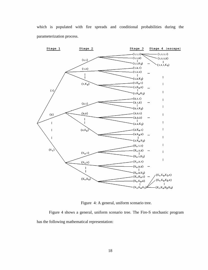
which is populated with fire spreads and conditional probabilities during the
parameterization process.
Figure 4: A general, uniform scenario tree.
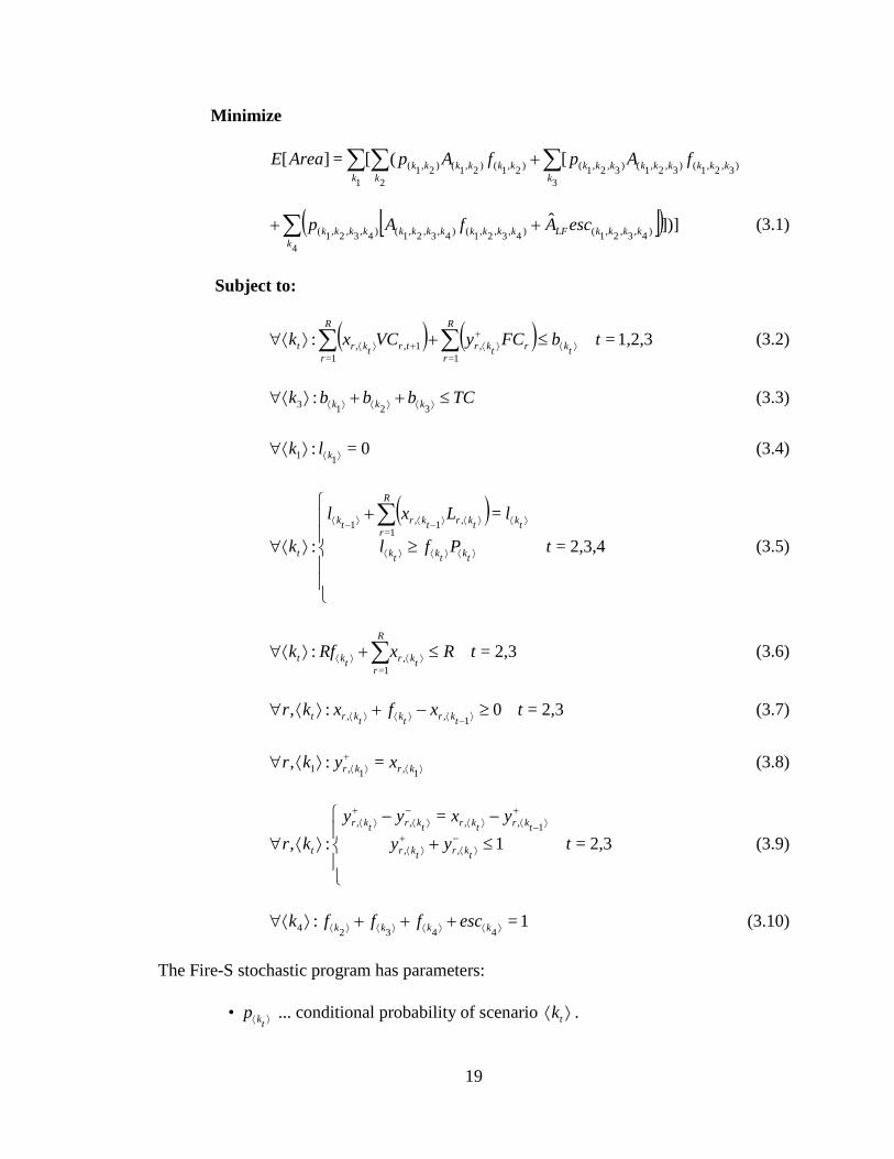
Figure 4 shows a general, uniform scenario tree. The Fire-S stochastic program
has the following mathematical representation:
19
Minimize
)3,2,1()3,2,1()3,2,1(
3
)2,1()2,1()2,1(
21
[([=][ kkkkkkkkkk
kkkkkkkk
fApfApAreaE ∑∑∑ +
[ ]( )])]ˆ)4,3,2,1()4,3,2,1()4,3,2,1()4,3,2,1(
4
kkkkLFkkkkkkkkkkkkk
escAfAp ++∑ (3.1)
Subject to:
( ) ( ) 1,2,3=: ,1=
1,,1=
tbFCyVCxktkrtkr
R
rtrtkr
R
rt ⟩⟨
+⟩⟨+⟩⟨ ≤+⟩∀⟨ ∑∑ (3.2)
TCbbbk kkk ≤++⟩∀⟨ ⟩⟨⟩⟨⟩⟨ 3213 : (3.3)
0=:11 ⟩⟨⟩∀⟨ klk (3.4)
( )2,3,4=
=
:,1,
1=1
tPfl
lLxl
ktktktk
tktkrtkr
R
rtk
t
≥
+
⟩∀⟨ ⟩⟨⟩⟨⟩⟨
⟩⟨⟩⟨⟩−⟨⟩−⟨ ∑ (3.5)
2,3=: ,1=
tRxRfktkr
R
rtkt ≤+⟩∀⟨ ⟩⟨⟩⟨ ∑ (3.6)
2,3=0:,1,, txfxkr
tkrtktkrt ≥−+⟩⟨∀ ⟩−⟨⟩⟨⟩⟨ (3.7)
⟩⟨+
⟩⟨⟩⟨∀1,1,1 =:, krkr xykr (3.8)
2,3=1=
:, ,,
1,,,,
tyyyxyy
krtkrtkr
tkrtkrtkrtkr
t
≤+
−−
⟩⟨∀ −⟩⟨
+⟩⟨
+⟩−⟨⟩⟨
−⟩⟨
+⟩⟨
(3.9)
1=:44324 ⟩⟨⟩⟨⟩⟨⟩⟨ +++⟩∀⟨ kkkk escfffk (3.10)
The Fire-S stochastic program has parameters:
• ⟩⟨ tkp ... conditional probability of scenario ⟩⟨ tk .

20
• ⟩⟨ tkP ... fire perimeter under scenario ⟩⟨ tk , cumulative through Stage t .
• ⟩⟨ tkA ... area burned under scenario ⟩⟨ tk , cumulative through Stage t .
• LFA ... estimated area of a large fire.
• R ... integer size of resource set.
• ⟩⟨ tkrL , ... line production during Stage t for resource r under scenario ⟩⟨ tk .
• trVC , ... variable cost of using resource r during Stage t .
• rFC ... fixed cost of dispatch for resource r .
• TC ... total budget for fire.
and decision variables:
• ⟩⟨ tkrx , ... binary, ``is resource r active on the fire (includes initial dispatch,
transit, and fire line construction) during Stage t under scenario ⟩⟨ tk ?''
• ⟩⟨ tkf ... binary, ``is containment first declared under scenario ⟩⟨ tk ?''
• ⟩⟨ tkry , ... binary, tracks initial deployment stage for resource r to determine
fixed cost payment.
• ⟩⟨ 4kesc ... binary, ``does fire escape under scenario ⟩⟨ 4k ?'' Indicates that the
fire was not contained in the scope of this model under scenario ⟩⟨ 4k .
• ⟩⟨ tkl ... book-keeping variable that tracks total line production under scenario
⟩⟨ tk .
• ⟩⟨ tkb ... ``how much of the budget is spent under scenario ⟩⟨ tk ?''
This is a mixed integer linear program with a size that depends upon the

21
underlying scenario tree. Endless variations of the general scenario tree in Figure 4 are
possible, so the Fire-S program has endless variations as well. The binary containment
variable is slightly tricky so we offer the following clarification:
• 1=⟩⟨ tkf if and only if the fire is declared contained during stage t under
scenario ⟩⟨ tk or
• 0=⟩⟨ tkf if and only if the fire is considered uncontained (or has been
previously contained) under scenario .⟩⟨ tk
The objective function in Equation (3.1) gives the expected burned area given all
the containment decisions. These calculations are discussed extensively in Section 2 and
Equations (2.6) and (3.1) are similar. The only difference is that (3.1) introduces the
possibility of fourth stage containment with ⟩⟨ 4kf whereas (2.6) assigns the expected
large fire area to any active fourth stage fire scenario. Note well that the areas are
cumulative, but given the tricky definition of ⟩⟨ tkf this does not lead to double counting.
We assume no line is built during Stage 1 so the fire must always grow into Stage 2,
which accounts for the abbreviated Stage 1 summation.
The constraints in (3.2) ensure variable and fixed costs for each scenario ( ⟩∀⟨ tk )
at each dispatch stage ( 1,2,=t and 3 ) are within budget. Notice that a resource deployed
during Stage t incurs the variable cost associated with Stage 1+t because we assume the
resource starts building line at the start of the stage immediately following its dispatch.
Fixed cost is incurred one time, if the resource is dispatched at all. While (3.2) is a
concise formulation, do not forget that it represents a set of many constraints, the number
of which depends upon the size of the underlying scenario tree. This is true for each set of

22
constraints (3.2) through (3.10).
Budget decision variables across dispatch stages are constrained to be less than
the total budget for each fire scenario in (3.3). The efficacy of our ⟨⋅⟩ notation is apparent
in (3.3) when we indicate ⟩∀⟨ 3k . Once some ⟩⟨ 3k is chosen, ⟩⟨ 1k and ⟩⟨ 2k are
automatically the proper parent scenarios. For example, suppose (3,4,2)=3⟩⟨k , which
indicates (3)=1⟩⟨k and (3,4)=2⟩⟨k . The corresponding constraint in (3.3) is
,(3,4,2)(3,4)(3) TCbbb ≤++
which indeed captures the budget decisions across the three dispatch stages for a given
scenario branch. It forces them to be less than the total allotment for the fire.
Constraints in (3.4) show the assumption that no line is built during Stage 1. Stage
1 is reserved for size-up and the initial call for resources.
The constraint pairs shown in (3.5) enforce classic containment. For each stage
where containment is possible ( 2,3,=t and 4 ) and each scenario ⟩⟨ tk , we permit
containment if and only if cumulative fire line production exceeds fire perimeter. Again,
observe that an active resource in Stage 1−t ( 1=1, ⟩−⟨ tkrx ) is assumed to produce line
during the following Stage t ( ⟩⟨ tkrL , ). The one stage lag allows for transit and prep time.
Notice the book-keeping variable ⟩⟨ tkl facilitates the computation of line accumulation.
The cumulative nature of (3.5) allows for multistage containment efforts, as discussed in
Section 2.
We refer to the set of constraints expressed in (3.6) and (3.7) as logical dispatch.
If the fire is declared contained under scenario ⟩⟨ tk ( 1=⟩⟨ tkf ), then no further resources
are dispatched and those resources already there are sent home according to (3.6). If a

23
resource is sent to a fire under scenario ⟩⟨ tk and the fire remains uncontained, the
appropriate constraint from (3.7) requires the resource to remain on the fire. These two
sets of constraints may be subject to tweaking based on a region's specific dispatch
routines. If, for example, the model's scope is much longer than two days, it may be
logical to permit resources to leave an uncontained fire and go to another fire, which
violates (3.7). An example exception to (3.6) would be if a fire manager wanted to
account for mop-up operations in planning. In which case, logical dispatch may involve
leaving a crew on a fire after it is declared contained. The Fire-S stochastic program must
be calibrated for the problem's scope and the region being modeled, which may include
slight changes in the constraints.
The set of constraints in (3.8) and (3.9) govern fixed cost payment. In (3.8), the
tracking variable +⟩⟨ 1, kry is initialized. We have utilized a linear programming trick from
[3] to detect a change from
1,=0= ,1, ⟩⟨+
⟩−⟨ tkrtkr xtoy
which indicates an initial dispatch of resource r in the variable +⟩⟨ 1, kry . This, in turn,
triggers fixed cost payment in the associated cost constraint in (3.2).
For each fire scenario, the associated constraint in (3.10) requires either the fire be
contained at some node of the scenario tree or escape the scope of the model. Again, we
see the convenience of the ⟨⋅⟩ notation in selecting branches that include appropriate
parents because these constraints could equivalently be written as
1.=:),,,( )4,3,2,1()4,3,2,1()3,2,1()2,1(4321 kkkkkkkkkkkkk escfffkkkk +++∀
As the Fire-S stochastic program is a potentially large, mixed integer program (MIP), we

24
solve it using ILOG CPLEX, a high powered linear program solver produced by IBM.
We detail the solution in Section 5.1. As the extensive parameter list asserts, there is
much background work to be done before the stochastic program can be passed to the
solver. Section 4 guides the reader through the parameterization process.
4 Parameterization
The Fire-S stochastic program in Section 3 reflects the richness and complexity of
the mathematics of decision-making, but the parameterization process gives the program
context in terms of fire behavior science and suppression resources. We simulate fire
behavior using Farsite. Fire simulation is fundamentally based on the Fire Triangle: fuels,
topography, and weather. In our study of the single-fire resource allocation for
suppression problem, topography is fixed because we elect a single ignition location in
the Black Hills National Forest (BHNF) in southwestern South Dakota. Fuels can be
considered mostly fixed because (a) the fire behavior fuel models are drawn from the
LANDFIRE database for the study area and (b) before we parameterize the model we
draw an ignition date from historical records, which fixes fuel moistures at their historical
levels. Weather may cause fuel moistures to vary because Farsite is capable of computing
dynamic fuel moistures during a simulation. Therefore, weather variables produce all the
variability in our probabilistic study. The parameterization process involves a cluster
analysis of historical weather data to produce representative weather streams with
associated conditional probabilities ⟩⟨ tkp . Each representative weather scenario seeds
Farsite to create a representative fire behavior scenario, which includes perimeter ⟩⟨ tkP
and area ⟩⟨ tkA parameters as output. We explain the cluster analysis in Section 4.1 and
25
tackle fire simulation in Section 4.2. The remaining parameters are associated with the
suppression resource set and are discussed in Section 4.3. Finally, we discuss escaped
fires in Section 4.4.
4.1 Cluster Analysis
Generating feasible weather scenarios from scratch is an enormous, multi-variate
correlation problem. We sidestep the problem by studying historical weather records. So
when a complicated correlation question arises---such as how the passage of a cold front
caused some irregular change in temperature, relative humidity, wind speed, and wind
direction---we can default to the fact that the weather pattern actually occurred and, save
some sort of data logging error, the weather variables are realistically correlated. While
this is a strong advantage, incorporating historical weather introduces some challenges.
The Western Regional Climate Center (WRCC) offers hourly data streams from Remote
Automated Weather Stations (RAWS), dating back to 1993 for some stations, in and
nearby the BHNF. In theory, we could run fire simulations for all possible combinations
of this historical weather and parameterize the Fire-S stochastic program with the output
using uniform probabilities, but such an approach would be unwieldy and time-
consuming. Instead, we use data clustering techniques to pre-process the weather records
and create weather classes from which to pull a few, representative weather scenarios.
The following discussion is specific to BHNF, but the basic steps can be modified to
apply to other locations as well.
Recall from Section 2 that at the outset of the Fire-S model, the fire manager has
no deterministic knowledge of weather or fire behavior. Once an ignition is reported,
important spatial and temporal information becomes immediately available. The fire

26
manager knows where, perhaps very roughly, the smoke is coming from and also knows
when the fire started. Not only are current weather conditions available, but forecast
information is quickly obtainable as well. To parameterize the conditional probabilities
⟩⟨ tkp in the Fire-S stochastic program, we seek to compare historical fire weather to the
forecast. We want to take into account types of weather that are historically likely and
types that are unlikely, but could lead to extreme fire behavior based on our simulations.
The first step we take from the large BHNF weather data set towards a small
subset of representative scenarios based on the forecast is to fix our spatial element by
electing a specific RAWS to use. For our analysis, Nemo was chosen as the best
representative for local fire weather based on proximity and similarity in elevation to our
ignition location in the Deerfield management zone [2]. Next, we apply a three month
filter to the historical records based on the ignition month. The filter screens out all data
except those records that match the ignition month, one month prior, or one month
following. For example, this filter avoids the issue of a July ignition somehow pulling a
February snow storm from the historical data. This technique is BHNF-specific; the
three-month filter works well for the BHNF, but may not work well in a region where
adjacent months have very different weather characteristics, if, for example, a monsoon
month interrupts the fire season. These two steps: a spatial fix and a month filter, greatly
reduce the size of the weather set and we call this starting set of weather records W .
In general, multi-variate clustering typically involves some sort of metric that
serves as the standard for comparison among vectors. For us, the question is: ``how far is
a given weather record from the forecast?'' There are many possible answers to this
question because there are many weather-related field observables. We elect to work with

27
vectors that consist of four weather variables: temperature ( temp ), relative humidity
( rh ), wind speed ( wspd ), and the cosine of wind direction ( wdircos ). This selection is,
of course, subjective and based on our experience with BHNF weather data in this
specific context; variations are numerous and many may be feasible as well. Let
( ) Wwdirwspdrhtemp iiii ∈cos,,,=iWx
be a weather vector in set W and let
( )0000 cos,,,= wdirwspdrhtempFx
be the forecast vector. To start, the forecast vector also comes from W . In Section 5.6 we
discuss some forecast considerations for the Fire-S model. Implicit in this discussion is
that these vectors come from a specific time of day because we work with hourly weather
data. In terms of the scope shown in Figure 1, there are morning and afternoon forecasts,
which we assume correspond to weather vectors at 1000 hours and 1400 hours
respectively. The fire manager may adjust these forecast points based on the burn period
and scope of the model. Our metric to compare iWx and Fx must account for all four
variables, their correlations, and their relative numeric sizes. As such, we compute the
44× covariance matrix S (and its inverse 1−S ) of temperature, relative humidity, wind
speed, and wind direction for all the data in set W . As a metric, we elect a generalized,
Euclidean distance measure
( ) ( ) ( ).=, 1 FxWxFxWxFxWx iii −−± −Sd T (4.1)
We call the scalar distances in Equation (4.1) forecast errors. By using the covariance
matrix in this way, we resolve correlation issues such as the strong negative correlation
between temperature and relative humidity. We also resolve relative numeric size issues

28
such as the differences in weather variable units. Equation (4.1) indicates the multi-
valued nature of the square root function in the ``± .'' While it is customary to pick the
positive square root for a distance measure, if we do this, there will be no distinction
between ``better'' and ``worse'' fire weather. For instance, a dry, windy iWx record could
map to the same forecast error numeric value as a wet, calm one. This happens quite
readily in fact. Suppose
( ) ( ),225cos,,25%,376=cos,,,= 0000 mphFwdirwspdrhtempFx (4.2)
( ),225cos,,42%,059= mphF148Wx (4.3)
( ),225cos,,8%,693= mphF643Wx (4.4)
and for the sake of simplicity assume no correlation and uniform covariance so that S
and 1−S are 44× identity matrices. Then, ( ) 24.2281=,FxWx148d and
( ) 24.2281.=,FxWx643d This is clearly a problem because when we simulate fire
behavior colder, wetter 148Wx will likely result in less severe fire behavior than drier,
windier 643Wx and we do not want them to fall into the same cluster. To circumvent this
issue we introduce a decision rule in order to establish clear separation between 148Wx
and 643Wx ; in general, we assign the negative square root to cooler, calmer weather
records and the positive square root to warmer, windier records. The rule manifests as a
comparison of the relative error (not to be confused with forecast error) in the relative
humidities and wind speeds of iWx and Fx ; compute

29
0
0=)(RH
RHRHRHerror ii
− (4.5)
and
,=)(0
0
wspdwspdwspdwspderror i
i− (4.6)
then make a decision according to the sign of the sum
( )( ) .
0<,0<)()(0,0)()(
FxWxFxWx
i
i
dwspderrorRHerrordwspderrorRHerror
ii
ii
+≥≥+
(4.7)
Let us examine how this decision rule applies to the example vectors from (4.2), (4.3),
and (4.4). From (4.5) we have 0.68=)( 148 −RHerror and 0.68=)( 643RHerror . From
(4.6) we have 1.0=)( 148 −wspderror and 1.0=)( 643wspderror . According to the rule in
(4.7) we assign the negative square root to 648Wx so that ( ) 22.2281=, −FxWx148d and
( ) 22.2281=,FxWx653d . This introduces a logical spacing in forecast errors, which helps
avoid automatic grouping of weather records that may in fact be dissimilar. One can
easily imagine loopholes and canonical cases for the decision rule in 4.7, but it serves as a
rough approximation and oftentimes when a questionable decision is made, we are
rescued by the next phase of clustering, which we will now describe.
The mathematical machinery of the metric (4.1) and associated decision rule (4.7)
combine to create a logical ordering of weather data. Given the set of weather vectors W
and a forecast vector Fx we can make the aforementioned assumptions and write a
roughly ordered list of forecast errors from least severe to most severe in terms of
expected fire behavior. An example of this ordering is shown in Table 3.

30
Table 3 1Wx 2Wx ... iWx ... MWx
June 23, 1995 August 8, 2009 ... July 10, 2003 ... July 25, 2002
Table 3: Example Stage 1 weather record ordering.
Smaller indices in Table 3 indicate cooler, wetter records where we expect more
mild fire behavior. Larger indices are indicative of more severe fire behavior because the
associated weather records are hotter and drier. Some weather record on the list will be
most similar to Fx , i.e. have the forecast error that is closest to 0. While each vector
iWx represents specific forecast values, each one corresponds to a date as shown the
second row of Table 3. Clearly, to order weather data like this, the dates are taken out of
their customary time ordering.
We propose a weather classification scheme to produce a coherent scenario tree
like the example from Section 2, which is shown in Figure 2. Our work will produce a
scenario tree, which is shown, in general, in Figure 4. Instead of having a rough idea of
pre and post-frontal weather patterns, the fire manager now has a vast cache of RAWS
data to create more detailed fire growth simulations. Even with the spatial (fixed ignition
location) and seasonal (month filter) simplifications used to create W , there still may be
a large number of weather records on this list. For the BHNF data 1000:M . Running
Farsite M times is certainly an option for the fire manager, but not a very practical and
interpretable one. Instead, we group similar weather records together in a hierarchical
clustering and select a representative weather scenario from each group. The fire
manager sets 1K to be the number of branches he or she wants from the initial node. A
hierarchical clustering algorithm starts with each record in its own group ( M groups)
and begins by pairing the two records that have the most similar forecast errors. On the

31
list, it replaces these two forecast errors with their average and then looks for the next
most similar pair of forecast errors. This will continue until there are 1K groups. For a
general description of this technique and some very informative diagrams consult [1].
Hierarchical clustering produces 1K subsets of W . Let WWk ⊆1
be the stk1
subset. For each 11 ,1,2,= Kk we select a representative scenario from 1kW . This could
be some sort of average weather record, a modal weather pattern, or some other type of
representative. We pick our stk1 representative scenario to be the record with the median
forecast error in 1kW . But, what probabilities, conditional and unconditional, does this
representative scenario carry? We create the Stage 1 probabilities ⟩⟨ 1kp and ⟩⟨ 1ˆ kp used to
parameterize the Fire-S stochastic program from the sizes of each subset. Computing
probabilities becomes a record counting endeavor. Let || ⋅ indicate the number of
elements in a subset. The Stage 1 node has no parent so the conditional and unconditional
probabilities are equal. We define
.||
=ˆ= 111 M
Wpp k
kk ⟩⟨⟩⟨
Notice that this definition is consistent with the two properties for the conditional
probabilities we pointed out in Section 2. Property (2.1) from Section 2 holds because
1,||
=<0 111 ≤⟩∀⟨ ⟩⟨ M
Wpk k
k
since 1kW has at least one (if it was never paired up) and at most M elements (if 1=1K ).
Property (2.2) from Section 2 holds because

32
1,=|=|1=||
=1
1
1=1
11
1=11
1
1=1MMW
MM
Wp k
K
k
kK
kk
K
k∑∑∑ ⟩⟨
since during the clustering algorithm every record in W is placed in some group. Thus,
each representative scenario is assigned a probability based on the size of the weather
record cluster that it represents. In terms of the scope of the Fire-S model shown in
Figure 1, each Stage 1 representative specifies which morning weather record use in the
Farsite simulation.
The next step in our clustering procedure is the key to conditionality in the Fire-S
model. With the representative weather record in place for the morning (Stage 1), we
must decide which weather record to simulate with in the afternoon (Stage 2). Fix the
number of Stage 2 branches from each node )( 12 ⟩⟨kK and apply the hierarchical
clustering algorithm to each Stage 1 subset. The result will be a collection of new subsets
WW k ⊆⟩⟨ 2 with the added property: ⟩⟨⟩⟨ ⊆
12 kk WW . Just as before, we select the median as
a representative scenario and assign it an unconditional probability based on group size:
.||
||=ˆ
1
22
⟩⟨
⟩⟨
⟩⟨k
kk W
Wp
To compute Stage 2 conditional probabilities we see
.||
=||
||
||
||=ˆ= 2
2
1
1
2122 M
W
W
W
W
Wppp k
k
k
k
kkkk
⟩⟨
⟩⟨
⟩⟨
⟩⟨
⟩⟨
⟩⟨⟩⟨⟩⟨ ⋅⋅
Conditionality is tracked using the sizes of the subsets. Once a weather record is collected
in a Stage 1 cluster, we do not allow it to change clusters. Suppose we derived a
representative scenario to be a member of W that was outside the parent subset. This
would violate the conditionality we are trying to establish. In general, the hierarchical
33
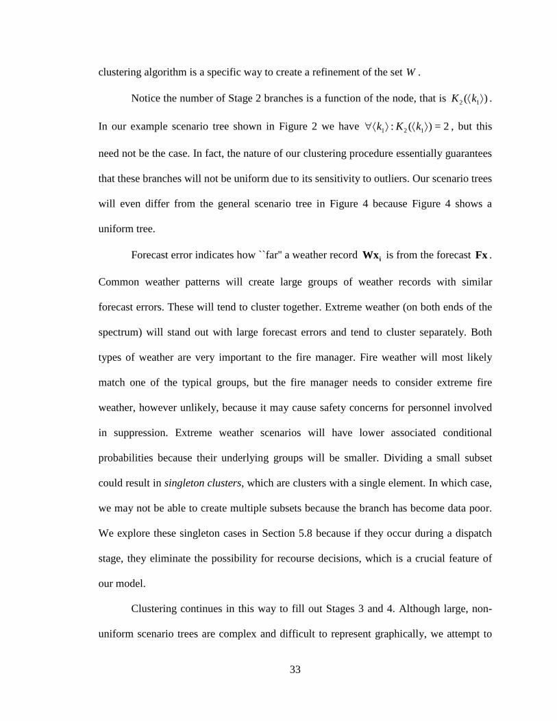
clustering algorithm is a specific way to create a refinement of the set W .
Notice the number of Stage 2 branches is a function of the node, that is )( 12 ⟩⟨kK .
In our example scenario tree shown in Figure 2 we have 2=)(: 121 ⟩⟨⟩∀⟨ kKk , but this
need not be the case. In fact, the nature of our clustering procedure essentially guarantees
that these branches will not be uniform due to its sensitivity to outliers. Our scenario trees
will even differ from the general scenario tree in Figure 4 because Figure 4 shows a
uniform tree.
Forecast error indicates how ``far'' a weather record iWx is from the forecast Fx .
Common weather patterns will create large groups of weather records with similar
forecast errors. These will tend to cluster together. Extreme weather (on both ends of the
spectrum) will stand out with large forecast errors and tend to cluster separately. Both
types of weather are very important to the fire manager. Fire weather will most likely
match one of the typical groups, but the fire manager needs to consider extreme fire
weather, however unlikely, because it may cause safety concerns for personnel involved
in suppression. Extreme weather scenarios will have lower associated conditional
probabilities because their underlying groups will be smaller. Dividing a small subset
could result in singleton clusters, which are clusters with a single element. In which case,
we may not be able to create multiple subsets because the branch has become data poor.
We explore these singleton cases in Section 5.8 because if they occur during a dispatch
stage, they eliminate the possibility for recourse decisions, which is a crucial feature of
our model.
Clustering continues in this way to fill out Stages 3 and 4. Although large, non-
uniform scenario trees are complex and difficult to represent graphically, we attempt to

34
do so in the exploded tree diagrams of Section 5.1. Each Stage 4321 →→→ path
),,,( 4321 kkkk specifies a weather stream. We form the stream by splicing four
representative weather records together. The dates will quite possibly be discontinuous.
Table 4 shows two examples of this splicing.
Table 4 Path Stage 1 Stage 2 Stage 3 Stage 4
(3,5,1,6) August 12, 2010 July 31, 1998 July 3, 2001 August 8, 2004 *(1,4,1,1) June 9, 2005 June 10, 1994 June 11, 1994 June 11, 1994
Table 4: Possible representative weather scenarios.
The path marked with a * indicates a singleton case. Starting at Stage 2 the same
record is being drawn as a representative because (1,4)W has a single member. This annuls
the multistage set-up of the Fire-S stochastic program because the Stage 3 and 4 weather
is known starting at Stage 2. Again, we refer the reader to Section 5.8 for a better
discussion.
Before we move onto simulation, let us study some features of the cluster analysis
procedure as applied to the BHNF data.
35
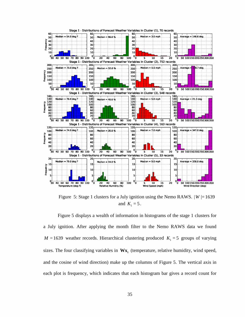
Figure 5: Stage 1 clusters for a July ignition using the Nemo RAWS. 1639|=|W and 5=1K .
Figure 5 displays a wealth of information in histograms of the stage 1 clusters for
a July ignition. After applying the month filter to the Nemo RAWS data we found
1639=M weather records. Hierarchical clustering produced 5=1K groups of varying
sizes. The four classifying variables in iWx (temperature, relative humidity, wind speed,
and the cosine of wind direction) make up the columns of Figure 5. The vertical axis in
each plot is frequency, which indicates that each histogram bar gives a record count for

36
the corresponding bin on the horizontal axis. For example, cluster (1)=)( 1k has a lot of
rainy days because of the 70 records in cluster (1) approximately 55 show relative
humidity near 100% . Figure 5 allows us to visually inspect the degree to which the
clustering technique accomplished our goals. Recall that our initial ordering established a
rough ranking system for fire weather. Greater indices were indicative of more severe fire
weather in terms of simulated fire behavior. As we collapsed the records into the
groupings shown in Figure 5, that relationship was maintained. If our classification
scheme worked, then we expect to find mildly severe fire weather in cluster (1)=)( 1k
and increasingly worse fire weather until cluster (5)=)( 1k , which should represent
extreme fire weather and behavior. Study the medians and distribution shapes for the
temperature, relative humidity and wind speed columns in Figure 5 and we see this is
indeed what occured. For example, consider wind speed. The medians increase from 3.0
mph to 9.0 mph monotonically from cluster (1)=)( 1k to (5)=)( 1k . Furthermore, the
distributions appear to trend towards higher wind speeds as well. Considering our desire
to separate cool, wet, and calm days from hot, dry, and windy using the metric in (4.1)
and decision rule in (4.7), Figure (5) is strong evidence in support of the cluster analysis
approach.
Thus far, we have not considered the wind direction column of Figure 5, but it
creates a somewhat different lens through which to view these fire weather clusters.
Recall that the analysis was performed on the cosine of wind direction, so these plots
represent the compass rose. For instance, at first glance the histogram of wind direction in
cluster (3)=)( 1k looks odd and strongly bimodal, but it actually reflects strong central
tendency about north or 0 . Two dominant wind directions emerge when you take this

37
linearization of the compass rose into account: north ( 0: ) and south-southeast ( 150: ).
Based on general wind patterns in this region of the country we expect that a north wind
represents the passage of a cold front near the RAWS station. The prevailing winds are
likely represented by the south-southeast spike. With this in mind, look again at Figure 5
and some general categorizations of fire weather become apparent. We offer an
explanation for these categories in Table 5.
Table 5 Cluster (1)=)( 1k Low prevailing winds; precipitation. Cluster (2)=)( 1k Stronger prevailing winds; higher temperatures. Cluster (3)=)( 1k Moderate frontal winds; similar temperatures to cluster (2)=)( 1k Cluster (4)=)( 1k Dry cold front; strong winds. Cluster (5)=)( 1k Very dry cold front; very high temperatures; strong winds.
Table 5: Interpretation of fire weather categories in Figure 5.
These categories should be viewed more as descriptors than rules. In terms fire
suppression however, such categories are highly meaningful because they follow the type
of discourse heard on a radio in the field. For instance, say fire weather predictions
indicate a dry cold front is to move through the area during the burn period. The fire
manager could decide to run detailed analysis based on historical weather patterns in
cluster (2)=)( 1k and cluster (4)=)( 1k to best approximate fire behavior during frontal
conditions. Notice that this model run consists of all available weather data. Even though
we use a specific forecast in the forecast error computation, this type of model run
reflects fire behavior prediction in absence of a forecast. We will further discuss
forecasting and the contrast between operational and planning models in Section 5.6. A
fire weather forecast would indicate which weather category from Table 5 to expect. The
fire manager would then run a restricted model in which he or she used just the historical

38
data from this category. By restricting the number of data records to allow, the scenario
tree would quickly become data poor. Since one of our goals is to explore recourse and
the probabilistic nature of this model, we elect to use all the data, which assumes a
forecast is unavailable.
With a description like Figure 5 in hand, we can critique our use of the median as
a representative for each cluster. Mean forecast error would not be a good candidate to
dictate the choice of representatives because these distributions are not normal. Most are
asymmetric to some degree and skewness is quite common. Selecting the median
assumes central tendency in these distributions, which is observable to be roughly the
case in Figure 5, without assuming normality. The median forecast error may not always
reflect the median of all four weather variables. For example, we may notice that our
representative for cluster (1)=)( 1k has a wind speed of 3.0 mph, but happens to have a
relative humidity of 31%, which is far from the median. Our hope is that selecting a
single representative using the median captures the basic category of weather, while
maintaining the natural variations associated with complicated weather interactions.
With a proxy for each cluster at each stage in place as well as the associated
probability parameters ⟩⟨ tkp for the Fire-S stochastic program, we are ready to simulate
fire behavior. We use Farsite to create the area ⟩⟨ tkA and perimeter ⟩⟨ tkP parameters in
Section 4.2.
4.2 Fire Simulation
Section 4.1 explains the procedure we use to create a scenario tree diagram. Each
),,,(= 43214 kkkkk ⟩⟨ path through the scenario tree represents a possible path through
39
reality. This path has a probability of ⟩⟨ 4kp of actually occurring. Each node is a decision
point and everything that occurs along the branches from one node to the next is dictated
by the historic weather record that was chosen as the representative. Refer to Table 4 for
two examples of these spliced weather streams. The reader may be slightly troubled by
issues of continuity that this splicing process creates. Butting weather records up against
each other like this violates the notion that hourly weather data should change gradually
in a smooth manner. This objection is valid, but becomes less relevant considering
Farsite's simulation environment.
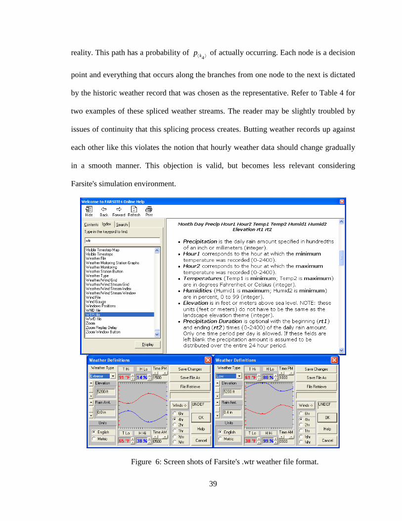
Figure 6: Screen shots of Farsite's .wtr weather file format.

40
Figure 6 shows Farsite's protocol for generating continuous weather streams for
simulation from a small set of inputs. Daily minima and maxima are used to create
sinusoidally varying weather on a daily basis. This technique helps smooth out
discontinuities in temperature and relative humidity. Hourly wind observations are
submitted and used directly in a Farsite simulation without this smoothing.
Discontinuities at nodes in wind behavior are less of a concern because winds tends to
change abruptly, at least more abruptly than temperature or relative humidity.
Farsite requires initial fuel moistures for 1-hour, 10-hour, 1000-hour, live
herbaceous, and live woody fuels. Once a smoke report is received, the fire manager will
be able to obtain or calculate these values appropriate to the ignition location. Farsite
incorporates a dynamic fuel moisture calculator that runs before the fire simulation. We
rely on Farsite to derive probabilistic fuel moisture scenarios from our probabilistic
weather scenarios.
Spatial data is not randomized. As noted in Section 4, once a smoke report is
made, the spatial aspects of the problem are fixed. We construct a landscape (.lcp) file
from LANDFIRE raster grid data for BHNF [10]. There are eight data layer requisites for
a landscape file:
1. Elevation
2. Slope
3. Aspect
4. Fuel Model (Scott and Burgan 40 from [11])
5. Canopy Cover
6. Stand Height
41
7. Crown Base Height
8. Crown Bulk Density
Each data input grid has 30 -meter resolution. The Northern Great Plains
Interagency Dispatch Center divides the BHNF into Initial Attack Response Zones.
Section O ``GPC Pre-planned Dispatch Cards'' of the 2006 Black Hills Fire Management
Plan [2] contains run cards that assign RAWS representatives to each zone. We simulate
a pixelated line of ignition in the Deerfield response zone, which relies on the Nemo
RAWS for initial weather data. Once a fire manager is managing a fire, he or she will
likely obtain more spatially specific weather data for fire behavior prediction, but at the
time of the smoke report, the RAWS data serve as the best available proxy for fire
weather.
We have two versions of the Farsite software with which to simulate fire
behavior. Farsite 4 is a free software package available from firemodels.org [6]. It has a
high-level, graphical user interface. It is enormously useful for single simulations, which
are important in the Fire-S calibration process. For example, to optimize computation
speed for large scenario trees, it is important to restrict the extent of the landscape file to
match the extent of the largest fires. Farsite's graphical interface is ideal for ironing out
these sorts of issues.
However, if the landscape is too small, the fire can move out of the grid and
render the perimeter and area parameters meaningless for larger fires. The second version
we have access to is a DLL that runs through an interface with the C programming
language. This version is enormously useful for the batch runs that are required to realize
a large-scale scenario tree, but less detail about each run is available. To achieve a batch
42
run we create weather scenario (.input) files for each path on the scenario tree; each
scenario file contains all the weather information required for the corresponding Farsite
simulation. The Farsite DLL creates grid files of simulation results. We derive ⟩⟨ tkA and
⟩⟨ tkP from these grids directly.
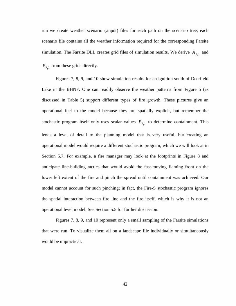
Figures 7, 8, 9, and 10 show simulation results for an ignition south of Deerfield
Lake in the BHNF. One can readily observe the weather patterns from Figure 5 (as
discussed in Table 5) support different types of fire growth. These pictures give an
operational feel to the model because they are spatially explicit, but remember the
stochastic program itself only uses scalar values ⟩⟨ tkP to determine containment. This
lends a level of detail to the planning model that is very useful, but creating an
operational model would require a different stochastic program, which we will look at in
Section 5.7. For example, a fire manager may look at the footprints in Figure 8 and
anticipate line-building tactics that would avoid the fast-moving flaming front on the
lower left extent of the fire and pinch the spread until containment was achieved. Our
model cannot account for such pinching; in fact, the Fire-S stochastic program ignores
the spatial interaction between fire line and the fire itself, which is why it is not an
operational level model. See Section 5.5 for further discussion.
Figures 7, 8, 9, and 10 represent only a small sampling of the Farsite simulations
that were run. To visualize them all on a landscape file individually or simultaneously
would be impractical.

43
Figure 7: Farsite simulation for (1,2,2,3)=4⟩⟨k . Wet cold front conditions.

44
Figure 8: Farsite simulation for (5,3,2,1)=4⟩⟨k . Dry cold front conditions; strong, north winds.
45
Figure 9: Farsite simulation for (6,3,3,2)=4⟩⟨k . Dry, prevailing conditions with high winds.

46
Figure 10: Farsite simulation for (2,2,2,4)=4⟩⟨k . Wet conditions turning dry and windy.

47
Figure 11: A probabilistic view of the fire behavior simulations in Farsite.
Instead, consider Figure 11. It shows a weighted scatter plot of the fire growth
parameters ⟩⟨ tkA and ⟩⟨ tkP . Probabilities are captured by the weight of the dots. We can
track typical fire growth by connecting large dots across the stages. We can track fringe
fire growth by connecting smaller dots. These are the scalar values that the Fire-S
stochastic program takes into account, which means it will be sensitive to all types of
simulated fire behavior.
Farsite also creates raster grids describing projected fire behavior such as flame
lengths, intensity, and rates of spread.

48
Figure 12: Probabilistic hauling charts.
Figure 12 displays some of this information in a probabilistic hauling chart
format. The fire manager can use such diagrams in combination with Appendix B of the
Fireline Handbook [7] or a software package like BehavePlus to assess fire severity and
address safety considerations under each fire behavior scenario. Consider Stage 4. Based
on the density of the points, it seems most likely that the fire will move from 5 to 10
meters per minute and create between 6 and 9 mega joules of heat per square meter.
However, there are fire behavior scenarios where the simulations show much more
extreme rates of spread and heats.
These simulations parameterize ⟩⟨ tkP and ⟩⟨ tkA in the Fire-S stochastic program.
The remaining parameters involve resources, financing, and escaped fire scenarios.
49
4.3 Suppression Resources
The Fire-S stochastic program exhibits enormous flexibility in terms of the
underlying resource set. Parameterizing the resources in the program is equivalent to
populating a table like Table 1 of Section 2. A fire manager must specify which resources
he or she has available and characterize their costs and line production rates.
To introduce fire suppression resource sets let us consider how the Fire-S
stochastic program formulation in (3.1) through (3.10) responds to small and large values
of R , or equivalently, small and large resource sets. Start with the extreme small case:
0=R . If there are no resources available to suppress a fire, the fire will grow in every
scenario. We will have 0=⟩⟨ tkf for every scenario ⟩⟨ tk at every stage t . As a result, the
set of constraints in (3.10) will indicate 1=4 ⟩⟨kesc for every ⟩⟨ 4k , which means every
fire behavior scenario escapes the scope of the model. The largest possible expected
burned area will be computed in the objective function (3.1). So in a sense, this
parameterization results in the worst possible optimal solution to our minimization
problem. As we increase R by adding resources to the available set, we expect to start
catching more and more fires and thus, lower the optimal expected burned area.
Next, let us explore the opposite extreme. Suppose R is huge. Say we
parameterize the Fire-S stochastic program with a national resource list that includes
every possible firefighting resource the fire manager could possibly obtain. This
parameterization will not result in zero expected burned area because our travel and prep
time assumption (3.4), that says 0=:,1,1 ⟩⟨⟩⟨∀ krlkr , will allow the fires to burn into stage
2 regardless of how many resources are deployed in Stage 1. Given the classic

50
containment constraints in (3.5) we might imagine such a large resource set to carry out
the most effective suppression possible under the travel time assumption and produce a
containment scenario where 1=2 ⟩⟨kf for every ⟩⟨ 2k . This type of total Stage 2
containment for all scenarios is certainly possible, but we need to take budget
considerations into account. Regardless of what is available in the resource set, the
program can only operate with resources it can afford based on the budget constraints in
(3.2) and (3.3). If R and TC are both huge, then total Stage 2 containment could occur.
The preceding discussion helps us to narrow down the size of the resource set to
use. In reality, the fire manager's budget will not be huge, but he or she will have
affordable suppression resources to work with. To reflect this reality we choose to make
R large to represent availability of resources, then restrict their use naturally with a
reasonable budget. A typical resource set is essentially an augmented version of Table 1
based on the approximate numbers of resources that the area has available. For the BHNF
we consult the Section M of the Fire Management Plan [2], which contains Most
Efficient Level forms.
Table 6 r Description Quantity FC ($) VC ($/hr) Rate (ch/hr) 1 Dozer 1 18,000 900 30 132− T6 Engine 12 8,000 400 16 1714− TI Hand Crew 4 2,050 250 9 2118− TII Hand Crew 4 1,000 100 3
Table 6: Resource set derived from MEL forms in BHNF Fire Management Plan
[2], 21=R .
Table 6 shows the working resource set that was derived from these forms. Notice
there are twelve identical Type 6 engines, four identical Type I hand crews, and four
identical Type II hand crews. Within these groups the linear solver will select an arbitrary

51
resource to use, but it may matter realistically which specific element is chosen. For
instance, if the model were updated to include prepositioning of resources or resource
travel time, beyond the current assumption of a single stage travel time, there could be
incentive to choose Engine B versus Engine K, if B was closer to the ignition than K, for
example. Also note that variable costs and line production rate estimates are given per
hour. The parameters trVC , and ⟩⟨ tkrL , should be scaled to be per stage, which will
depend on the scope of the model. We refer the reader to Section 2 for an example of
scaling from hourly to per-stage variable cost, but we delve deeper into the line
production parameter here.
Line production rates are approximated from guidelines in Appendix A of the
Fireline Handbook [7]. We assume line production is performed at the given rate during
the stage regardless of terrain, current fire behavior, and fatigue level of resources. Given
all that happens on a fire line, this is a broad assumption. Even the simplest factors, such
as slope or rocky soil, can greatly affect line production rates. These broad assumptions
are presumed to be acceptable at the planning level, but unacceptable at the operational
level. In planning, the interactions can be estimated, and we discuss options for doing so
in Section 5.5, to further the realism of the model. In operation, this model would need to
address such interactions in a more rigorous way because sometimes they are critical to
firefighter safety. We operate the model by assuming ⟩⟨ tkrL , could be expressed as trL , ,
but leave the scenario dependence notation to demonstrate the possibility of scenario-by-
scenario adjustment (see Section 5.5). Remember the Fire-S model has twelve-hour
stages, but we assume an eight-hour line building period within each stage. This
assumption accounts for resource positioning, fatigue, breaks, and other logistics.

52
4.4 Escaped Fires
All of the Fire-S stochastic program's parameters, as listed in Section 3, have been
filled save one. Section 2 gives a discussion of escaped fires defining them as fire
behavior scenarios that escape the predictive scope of the model. Recall that these are not
necessarily large fires, just longer-lasting than the two-day, four-stage scope of the Fire-S
model. Such fires must be accounted for in the objective function because it seeks to
minimize burned area and an escaped fire will likely have a significant contribution to
this value. As described in Section 2, the user supplies an estimate for an escaped fire
LFA . We set LFA to be an area estimate of a large fire in the BHNF because if the
program does not contain the fire, then it has continued to grow. Our best estimate for the
fire's area after it escapes the model's scope must assume the growth continues. One
possible way to derive this estimate is to use a Fire Family Plus database to calculate the
average fire areas from its top four size classes (D, E, F, and G). This method applied to
the BHNF database yields 7,814=ˆLFA ha, which, for reference, is about 20,000 acres.
Equation (3.1) shows how LFA is associated with the decision variables ⟩⟨ 4kesc to add
this escaped fire estimate to the expected area burned in the objective function.
5 Discussion
We will conclude this paper with a detailed discussion of the Fire-S model
outputs (Section 5.1). We examine outputs in general and then track a specific scenario
through the model. The Fire-S model is applied to a suppression budget analysis in
Section 5.2. We use two different model versions and the suppression budget analysis to
explore the advantages of complexity of the model in terms of better optimal solutions in

53
Sections 5.3 and 5.4. The remaining sections suggest avenues of continued exploration.
In reading through the results, we urge the reader to keep in mind that this is a ``proof-of-
method'' type paper as opposed to one designed to answer a specific research question so
that he or she can critique the model itself instead of focusing on the results.
5.1 Stochastic Program Outputs As we pointed out in Section 3, the Fire-S stochastic program is a large size,
mixed integer program (MIP). To give the reader an idea of how large it can get, consider
a uniform scenario tree (like Figure 4) with 4=== 41 KK that utilizes the resource set
in Table 6 where 21=R . A program of this size would have 5,884 decision variables
and 13,216 constraints in the formulation expressed in Equations (3.1) through (3.10)
from Section 3. This is a useful size considering the program that results from the cluster
analysis parameterization with Stage 1 shown in Figure 5 ran with 6,838 decision
variables and 7,308 constraints.
Despite their large sizes, these programs can be solved extremely quickly using
the high-powered linear solver CPLEX. CPLEX is distributed by IBM and incorporates
state-of-the-art branch-and-cut methods in its MIP solver. The user is further empowered
in terms of computing time with the ability to set relative error tolerances for solutions.
As such, these programs can be solved and studied relatively quickly. Each solver routine
is seeded with a ``.lp'' file, which contains the entire program with numerical values for
all its parameters. CPLEX outputs a wealth of information about the optimal solution of
the stochastic program. Solution diagnostics and the objective function value can be
printed. With our C-interface version of CPLEX a ``.sol'' solution file is written for each
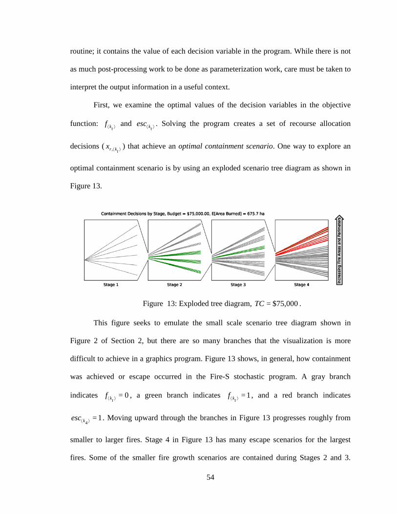
54
routine; it contains the value of each decision variable in the program. While there is not
as much post-processing work to be done as parameterization work, care must be taken to
interpret the output information in a useful context.
First, we examine the optimal values of the decision variables in the objective
function: ⟩⟨ tkf and ⟩⟨ tkesc . Solving the program creates a set of recourse allocation
decisions ( ⟩⟨ tkrx , ) that achieve an optimal containment scenario. One way to explore an
optimal containment scenario is by using an exploded scenario tree diagram as shown in
Figure 13.
Figure 13: Exploded tree diagram, $75,000=TC .
This figure seeks to emulate the small scale scenario tree diagram shown in
Figure 2 of Section 2, but there are so many branches that the visualization is more
difficult to achieve in a graphics program. Figure 13 shows, in general, how containment
was achieved or escape occurred in the Fire-S stochastic program. A gray branch
indicates 0=⟩⟨ tkf , a green branch indicates 1=⟩⟨ tkf , and a red branch indicates
1=4 ⟩⟨kesc . Moving upward through the branches in Figure 13 progresses roughly from
smaller to larger fires. Stage 4 in Figure 13 has many escape scenarios for the largest
fires. Some of the smaller fire growth scenarios are contained during Stages 2 and 3.

55
There are also fourth stage containments, but very few of them. Notice the model has
performed in accordance with our assumption in (3.4) that no Stage 1 containment is
possible. We will return to the exploded tree diagram as a tool to study the budget
constraint in Section 5.2.
The objective function value and budget constraint level are also printed in Figure
13. These indicate that given a budget of $75,000=TC to spend on fire suppression
resources, the fire manager can expect a minimum burned area of 675.7 ha. The next
logical question to ask is: under each scenario, which resources from Table 6 were
dispatched to suppress the fire and when were they ordered?
Table 7
r Description Stage 1 Stage 2 Stage 3 1 Dozer 16.7 % 0.0 % 0.0 % 2 T6 Engine A 16.7 % 12.5 % 13.5 % 3 T6 Engine B 16.7 % 4.2 % 4.1 % 4 T6 Engine C 16.7 % 4.2 % 5.4 % 5 T6 Engine D 0.0 % 0.0 % 0.0 % 6 T6 Engine E 33.3 % 0.0 % 0.0 % 7 T6 Engine F 0.0 % 4.2 % 4.1 % 8 T6 Engine G 0.0 % 0.0 % 0.0 % 9 T6 Engine H 0.0 % 0.0 % 0.0 %
10 T6 Engine I 16.7 % 4.2 % 4.1 % 11 T6 Engine J 50.0 % 16.7 % 4.1 % 12 T6 Engine K 66.7 % 16.7 % 4.1 % 13 T6 Engine L 50.0 % 0.0 % 0.0 % 14 T1 Hand Crew A 33.3 % 29.2 % 17.6 % 15 T1 Hand Crew B 16.7 % 29.2 % 20.3 % 16 T1 Hand Crew C 16.7 % 29.2 % 17.6 % 17 T1 Hand Crew D 16.7 % 29.2 % 17.6 % 18 T2 Hand Crew A 0.0 % 4.2 % 4.1 % 19 T2 Hand Crew B 0.0 % 4.2 % 5.4 % 20 T2 Hand Crew C 0.0 % 8.3 % 8.1 % 21 T2 Hand Crew D 0.0 % 4.2 % 5.4 %
Table 7: Resource dispatch and use rates. $75,000=TC , minimum expected
burned area = 675.7 ha, 22.2% of fire scenarios escape.

56
The most straightforward answer to this question is to tabulate how often each
resource is used during each stage across all scenarios. Table 7 shows just that. The
tabulated values indicate the percentage of ⟩⟨ tk for which 1=, ⟩⟨ tkrx . For example, we see
Type 6 Engine K ( 12=r ) was used in 66.7% of scenarios in Stage 1, then used in 16.7%
during Stage 2, and then used in 4.1% during Stage 3. Recall, that this indicates the
engine was on the fire and constructing line during Stages 2, 3 and 4 for those
percentages of scenarios. There are two factors that can cause the percentages to decrease
for this engine. One, the number of scenarios increases as the scenario tree branches out.
Two, some of the stages acheived containment so the engine was sent home. Table 7 is
ambiguous as to which was the true case. Overall, Table 7 should be viewed as a
summary of the overall tendencies of the dispatch decisions. It can guide further
investigation into the actual values of decision variables specific to a resource of interest.
For instance, suppose we are interested the resource prescription for scenario
(6,2,4,1)=⟩⟨ tk . For the ignition in the BHNF's Deerfield zone, the stochastic program
found fourth stage containment to be optimal, that is 1=(6,2,4,1)f . Let us examine this
scenario closely and dissect the model's performance in this specific case.
Scenario (6,2,4,1) can be deemed fringe fire behavior because it has a very low
conditional probability 4(6,2,4,1) 106.1= −×p . Nonetheless, it represents a possible weather
stream under the cluster analysis of the Nemo RAWS historical data so a simulation was
performed.

57
Table 8 Stage Weather Record
1 August 12, 2003 2 August 31, 2002 3 June 23, 2001 4 June 23, 2001
Table 8: Date splice description for scenario (6,2,4,1) .
Table 8 shows the date records that were spliced together as a representative for
the weather patterns found with the cluster analysis. We notice right away that this is
likely a singleton cluster in stage 3 because stage 3 and 4 share a date record. Next, let us
examine the RAWS data directly to describe the weather during the simulation.
Figure 14 plots hourly measurements of temperature, relative humidity, and winds
for scenario (6,2,4,1) . There was no precipitation recorded. The data show the typical
negative correlation of temperature and relative humidity. This weather stream shows
hot, dry, prevailing winds dominate the burn periods of both days. The winds are stronger
the first day than the second. A fire manager may be troubled when he or she sees the
wind plot of Figure 14 because it shows some significant changes in wind direction
throughout the day. This could be a common, up-slope/down-slope diurnal pattern, but
needs to be noted for firefighter safety. The Farsite simulation associated with this
weather scenario is shown in Figure 15.
The fire footprint does not give any strong clues about the driving weather, but
the fire front seems to be pushed by northerly winds and moves quite quickly during the
hot dry portions of each day. Farsite output also indicates torching, but the majority of the
fire is confined to surface spread.

58
Figure 14: RAWS data for (6,2,4,1)=⟩⟨ tk .
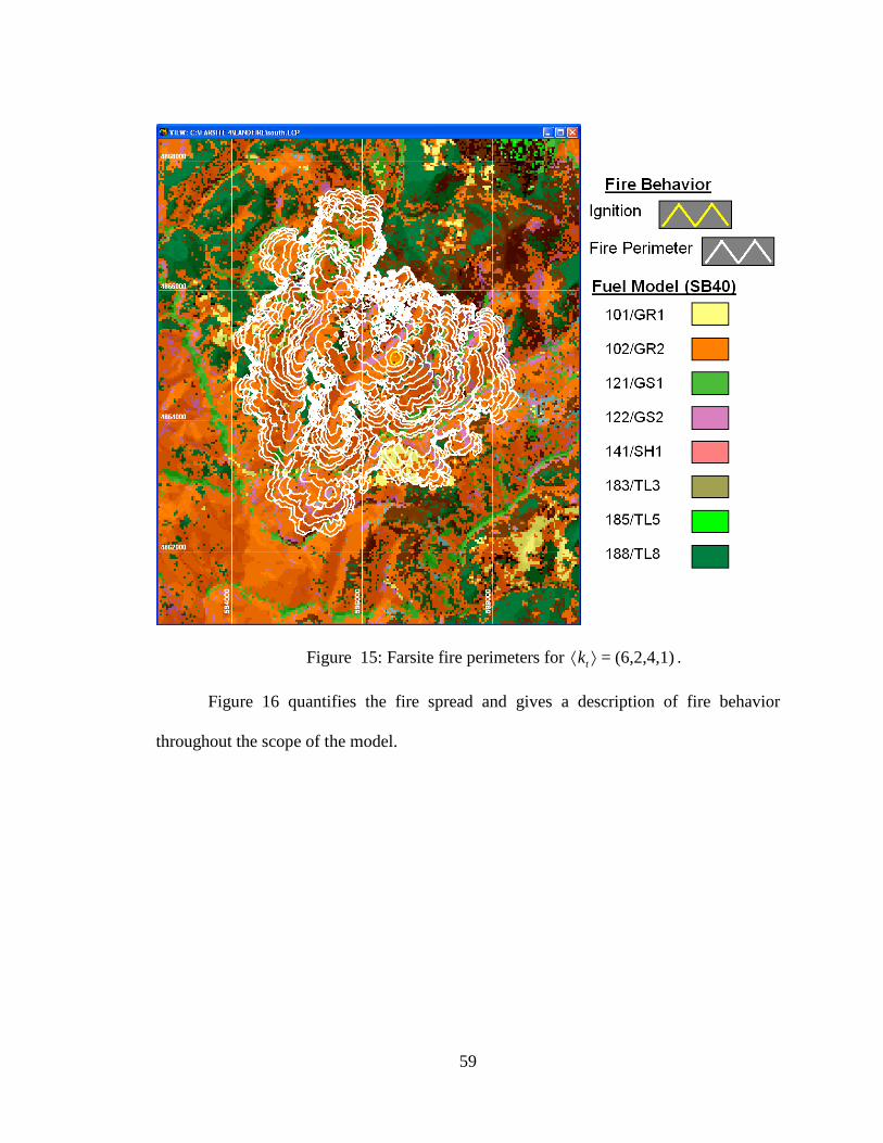
59
Figure 15: Farsite fire perimeters for (6,2,4,1)=⟩⟨ tk .
Figure 16 quantifies the fire spread and gives a description of fire behavior
throughout the scope of the model.
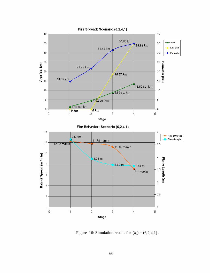
60
Figure 16: Simulation results for (6,2,4,1)=⟩⟨ tk .

61
Now that we have a rigorous description of the weather stream and resulting fire
behavior in scenario (6,2,4,1) , let us examine what the stochastic program outputs show
as the optimal resources to achieve 1=(6,2,4,1)f . Figure 16 also shows the progress of the
resources as they build line. We see that fourth stage containment is achieved by a very
small margin; the resources achieve 34.94 km of line at the end of Stage 4, which just
barely exceeds the Stage 4 fire perimeter of 34.86 km.
Table 9 Stage Package Description Cost
1 }{= ∅r No resources $ 0 2 ,16,17,20}{2,4,14,15=r Two engines, five hand crews $40,400 3 20},16,17,18,{2,4,14,15=r Two engines, six hand crews $17,000
Table 9: Dispatch packages for scenario (6,2,4,1) .
Table 9 shows the resources that were used for containment. With the budget of
$75,000=TC these dispatch packages were affordable because they cost $57,400. At
this point, we can critique the Fire-S program's choices. Sending so many hand crews
may be slightly illogical unless the fire is in rough terrain, which the program would have
no way of discerning. Likewise, we can make some comments about the practicality of
the line-building tasks. Building 35 km of lines would take considerable time, but to be
commensurate with fire sizes that is the required amount. We can imagine ``line
building'' to be a loose term and assume it includes natural barriers, but again, the
program itself has no way of knowing the spatial aspects of the problem. Issues such as
these indicate the importance of tight, overall calibration so that the outputs are as
realistic as possible.
A fire manager can use these outputs in many ways, but the context of a fire
planning model should always be considered. The level of detail in terms of stage-by-

62
stage decision-making and specific resource packages is a benefit of the Fire-S stochastic
program's formulation. But, as we have already mentioned and indeed will explore again
in Section 5.7, to make this model function on an operational level, we would need to
account for interactions between the fire and suppression resources. Section 5.2 proposes
a study that fits well in the planning framework.
5.2 Suppression Budget Analysis
As a fire planning model, this approach lends itself to suppression budget
planning. This type of analysis is routinely carried out using deterministic models, but the
appeal of using such a detailed, stochastic model is great. We run the Fire-S stochastic
program with various values of the TC parameter to show fire suppression performance
at different levels of the budget constraint in (3.3).
Figure 17 demonstrates the efficacy of the exploded tree diagram that we
mentioned in Section 5.1. The results in Figure 17 are created by finding four separate
solutions to the Fire-S stochastic program with budget constraint levels of $20,000,
$60,000, $75,000, and $150,000. First, notice the escaped fire branches decrease as the
budget constraint level is relaxed. More money means more containment options are
available because more resources can be dispatched. We also see a general trend towards
early containment, for scenarios that can be contained. More money allows more
resources to be dispatched right away to a fire and thus, lower the expected burned area.
The spectrum ranges from $20,000=TC , which displays limited third stage
containment, to $150,000=TC , which displays total Stage 2 containment.

63
Figure 17: Exploded tree diagrams with four levels of TC parameter.
We can further elucidate the relationship between suppression performance, as
captured in the objective function value, and the level of the budget constraint by solving
the Fire-S stochastic program for many values of TC .
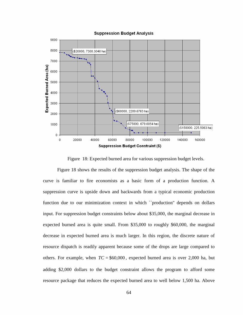
64
Figure 18: Expected burned area for various suppression budget levels.
Figure 18 shows the results of the suppression budget analysis. The shape of the
curve is familiar to fire economists as a basic form of a production function. A
suppression curve is upside down and backwards from a typical economic production
function due to our minimization context in which ``production'' depends on dollars
input. For suppression budget constraints below about $35,000, the marginal decrease in
expected burned area is quite small. From $35,000 to roughly $60,000, the marginal
decrease in expected burned area is much larger. In this region, the discrete nature of
resource dispatch is readily apparent because some of the drops are large compared to
others. For example, when $60,000=TC , expected burned area is over 2,000 ha, but
adding $2,000 dollars to the budget constraint allows the program to afford some
resource package that reduces the expected burned area to well below 1,500 ha. Above

65
$60,000 marginal decrease in expected burned area becomes nominal because we are
moving towards total Stage 2 containment and the model cannot perform any better. A
suppression curve like Figure 18 is a fundamental fire planning tool and can help
demonstrate budget requirements to funding agencies. For an ignition in the Deerfield
zone, a fire manager may want to realize an area-based suppression goal of 3,000 to
4,000 ha and can use this simulation, in combination with others if necessary, to justify a
budget request of $55,000 for the fire. Since a planning process makes more sense on a
seasonal level, we will discuss options for a multiple fire version of the Fire-S model in
Section 5.8.
5.3 Version Without Recourse
Not only is the statement in Section 3 of the Fire-S stochastic program
complicated, but the entire parameterization process discussed at length in Section 4 is
complex. All the complications arise from the multistage stochastic program formulation
with recourse, but what benefit, if any, does the complexity afford? We study the results
of a program without recourse and then one without multiple stages to study this question
in the context of our specific BHNF ignition. The suppression budget analysis of Section
5.2 provides a wonderful venue to compare these two variations with the full model.
To make each of these variations we start with the stochastic program in (3.1)
through (3.10) and add an extra set of constraints in each case. A common theorem from
[3] says that adding constraints to a math program cannot result in a better optimal
solution. So neither of these versions will lower expected burned area, but the exercises
are informative nonetheless because we can study the extent of the worsening in the
optimal solutions.

66
To start, let us eliminate the possibility for recourse decisions. By definition, a
recourse decision gets made after some random event is realized. In our case, the random
events are fire perimeters and in each Stage t we realize many perimeters ⟩⟨ tkP with
different conditional probabilities ⟩⟨ tkp . In order to disallow recourse, we must enforce an
extra set of constraints that require all dispatch decisions to be the same for each stage. In
other words, the fire manager is allowed to know the probabilities ⟩⟨ tkp , but must make
only one set of dispatch decisions at each stage. Given t , we force ⟩⟨ tkrx , to be the same
for each ⟩⟨ tk . For example, in Stage 1
.===: )1(,(2),(1), Krrr xxxr ∀
In Stage 2, the constraints become more complicated so we will state them as well:
∀
)2,1(,,2)1(,,1)1(,
)2(2,,(2,2),(2,1),
)2(1,,(1,2),(1,1),
====
=======
:
KKrKrKr
Krrr
Krrr
xxx
xxxxxx
r
An analogous set of constraints is added to make Stage 3 dispatch decisions uniform too.
The parameterization is exactly the same as the full model. We solve the Fire-S
stochastic program for various levels of the TC just as in Section 5.2. Results are shown
in Figure 19. We will discuss them after presenting the single stage version in Section
5.4.
5.4 Single Stage Version
Next, let us implement an extra set of constraints that eliminate the opportunity to
make distinct, stage-specific dispatch decisions. Equations (3.1) through (3.10) allow the

67
the fire manager to make distinct decisions at each node along a branch. We can turn the
program into a single stage version by forcing all dispatch decisions along each branch to
match. In this version the fire manager can still see the entire tree, but the decisions will
be made for the duration of the model right after Stage 1, following the smoke report.
Single-stage recourse still applies because decisions will be made based on the simulation
outcomes and their associated probabilities ⟩⟨ tkp . The extra set of constraints force ⟩⟨ tkrx ,
to be the same for each t . These constraints can be written
.==:,3,2,1,3 ⟩⟨⟩⟨⟩⟨⟩⟨∀ krkrkr xxxkr
Using a branch from Figure 2 as an example the constraint is
.==: (2,1,2),(2,1),(2), rrr xxxr∀
We implement this set of constraints and perform the budget analysis described in
Section 5.2.
Figure 19: Suppression budget analysis for restricted models.

68
Figure 19 shows the results of the comparison between the full model and both
restricted versions. Let us first consider the extremities of these curves. All models tend
to perform about the same for the region below $35,000. For small budgets, dispatch is
choked by lack of funds, so the complications of the full model are not a significant
advantage. Above about $85,000 recourse is not a factor because we are observing total
Stage 2 containment so recourse lends no significant advantage to the program. We see
the single stage version of the model does not reach the same total Stage 2 containment
floor after $85,000 as the other two versions. This is somewhat of a fabrication due to the
set of constraints in (3.7). If we force dispatch decisions to be the same along each
branch, then the constraints in (3.7) forbid Stage 2 and Stage 3 containment scenarios. On
one hand, this is exactly what we want to assume for a single stage version because we
cannot have staged decisions, which includes declaring containment before the end of
model. On the other hand, this is not very realistic. To study a single stage model, we
would most likely work with one of shorter duration, given the amount of detail we
incorporate in the program. Regardless, the tail of the single stage version's suppression
curve reflects total Stage 4 containment, as opposed to total Stage 2 containment.
Next, consider the region from $35,000 to $85,000 where the curves diverge. The
full model shows no clear advantage over the one without recourse until about $55,000.
At this point the optimal solutions without recourse are consistently higher expected
burned areas than the full model until total Stage 2 containment can be achieved at
$85,000. This is strong support, in this specific case and context, for recourse. Recourse
gives the program an ability to navigate alternatives when there are many to choose from.
In this region, there is sufficient budget money available to realize a wide variety of

69
containment scenarios without total Stage 2 containment. Letting the model make
recourse decisions according to typical and fringe fire behaviors allows for a more
accurate and possibly realistic reflection of the spectrum of suppression tasks. Whether or
not this is an advantage for the fire manager during the planning process becomes a
question of specificity of planning instead of modeling limitations.
The single stage version begins to lag near $35,000, catches up at $40,000, lags
again, catches up at $50,000 or so, and then lags for all higher values of TC . We can
interpret this as an indication of the advantage of multiple stages in this type of model.
When a single dispatch is made, there will be losses when the fire grows rapidly in the
late stages of the model. According to Figure 19 these losses outweigh the gains of
simultaneously preparing for all typical and fringe fire behaviors in a single dispatch. The
flexibility of a multistage decision process is apparent.
Figure 19 and the associated discussion represent a single case study, which is
insufficient to make conclusions about the methods described in this model in general. In
this case, the added complexity of multiple stages and recourse do change outputs. If we
assume multiple stages and recourse increase the realism of the model, then this allows us
to conclude, in this case, that the added complexity exhibits strong gains.
5.5 Interactions
Thus far we have alluded to interactions as an important component of the
resource allocation for fire suppression problem by noting this formulation lacks an
interaction term. We will explore why an interaction term introduces a greater level of
complexity in the model and suggest two ways to capture interactions within the current
framework.

70
Recall the classic containment constraints in (3.4) and (3.5) of Section 3. We
initialize line-building with the assumption
0,=:11 ⟩⟨⟩∀⟨ klk
track line production for 2,3=t and 4 with the book-keeping variable ⟩⟨ tkl using
( ) ,=: ,1,1=
1 ⟩⟨⟩⟨⟩−⟨⟩−⟨ ∑+⟩∀⟨tktkrtkr
R
rtkt lLxlk
and then decide containment for 2,3=t and 4 based on the following set of constraints
.: ⟩⟨⟩⟨⟩⟨ ≥⟩∀⟨tktktkt Pflk (5.1)
Say we want to include an interaction between line production and fire spread. We seek
some function g that gives the interaction between ⟩⟨ tkl and ⟩⟨ tkP so that we have an
adjusted estimate for perimeter ⟩⟨ tkP based on what the suppression resources have
previously done on the fire. In other words,
( ).,ˆ,=ˆ11 ⟩−⟨⟩−⟨⟩⟨⟩⟨ tktktktk lPPgP
There are countless ways to create the function g , all with varying levels of complexity.
We will explore a relatively simple choice. Suppose we approximate the interaction by
assuming line production decreases fire perimeter according to some scalar attack
parameter )(tα that describes the effectiveness of line building at each Stage t . This
allows us to create a family of functions )(tgα to describe the interaction:
( )⟩−⟨⟩−⟨⟩⟨⟩⟨ 11)( ,ˆ,=ˆtktktkttk lPPgP α
.ˆ)(ˆ
ˆ>)()(=
111
111
≤⋅−
⋅−⋅−
⟩−⟨⟩−⟨⟩⟨⟩−⟨
⟩−⟨⟩−⟨⟩⟨⟩−⟨⟩⟨
tktktktk
tktktktktk
PltPifP
PltPifltP
α
αα (5.2)

71
The function )(tgα is piecewise so that we do not somehow decrease fire perimeter from
one stage to the next. For this discussion we will assume )(tα is small enough that the
top option in (5.2) holds. For example, take 0.2=)(tα for each Stage t and say the fire
simulation shows a spread from 6.6=ˆ1⟩−⟨ tkP km to 10.3=⟩⟨ tkP km. If we allocate enough
resources to build 5.2=1⟩−⟨ tkl km of line, then the adjusted perimeter would be
.9.26=5.20.210.3=5.2)(10.3,6.6,=ˆ0.2 kmgP
tk ⋅−⟩⟨
In this way, we could continuously adjust the fire perimeters as the model progresses.
These ideas are sound, but implementing the model with ⟩⟨ tkP in place of ⟩⟨ tkP has
two critical pitfalls. First, in Farsite we simulate fire spread without line interaction.
Farsite does contain the features to implement barriers that act as fire line, but this would
complicate simulation immensely. We saw in Section 4 that the parameterization process
is spatially explicit, so line building parameters would also have to be spatially explicit,
which means careful consideration of terrain, fuel model, and strategy. We could choose
to be ignorant of this pitfall and work with the attack parameter )(tα to avoid
complicating the fire simulation process, but the second pitfall remains.
The second pitfall is that even this simple treatment of interaction introduces a
non-linearity in the set of constraints from (3.5). Suppose we substitute ⟩⟨ tkP for ⟩⟨ tkP in
(5.1). Then we have
⟩⟨⟩⟨⟩⟨ ≥⟩∀⟨tktktkt Pflk ˆ:
( )⟩−⟨⟩⟨⟩⟨ ⋅−1
)(=tktktk ltPf α
.)(=1⟩−⟨⟩⟨⟩⟨⟩⟨ −
tktktktk lftPf α (5.3)
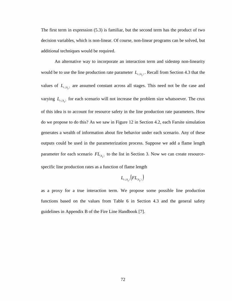
72
The first term in expression (5.3) is familiar, but the second term has the product of two
decision variables, which is non-linear. Of course, non-linear programs can be solved, but
additional techniques would be required.
An alternative way to incorporate an interaction term and sidestep non-linearity
would be to use the line production rate parameter ⟩⟨ tkrL , . Recall from Section 4.3 that the
values of ⟩⟨ tkrL , are assumed constant across all stages. This need not be the case and
varying ⟩⟨ tkrL , for each scenario will not increase the problem size whatsoever. The crux
of this idea is to account for resource safety in the line production rate parameters. How
do we propose to do this? As we saw in Figure 12 in Section 4.2, each Farsite simulation
generates a wealth of information about fire behavior under each scenario. Any of these
outputs could be used in the parameterization process. Suppose we add a flame length
parameter for each scenario ⟩⟨ tkFL to the list in Section 3. Now we can create resource-
specific line production rates as a function of flame length
( )⟩⟨⟩⟨ tktkr FLL ,
as a proxy for a true interaction term. We propose some possible line production
functions based on the values from Table 6 in Section 4.3 and the general safety
guidelines in Appendix B of the Fire Line Handbook [7].

73
Figure 20: Hypothetical line rates as a function of flame length.
Figure 20 shows a hypothetical example for a Type I hand crew, a Type 6 engine,
and a Single Engine Air Tanker (SEAT). Each resource has a maximum production rate
at which it builds line under practical and safe conditions. A hand crew might be able to
build line for low flame lengths, but then their abilities taper as the fire becomes more
intense until some threshold, shown in Figure 20 to be about 2.5 meters or about 8 feet,
where they must leave the fire line for safety. An engine can produce longer, but at lower
and lower rates as flame length increases. Although we have not included aircraft in our
exploration, a SEAT is shown in Figure 20 as well. It may not be practical to use such an
aircraft on small fires, but it is immediately and highly effective at some threshold flame
length and can be used until fire behavior becomes extreme.

74
Using flame length is a simple demonstration, but any combination of fuels,
weather, and topographic information could be combined to scale ⟩⟨ tkrL , . This would be
an incredibly interesting avenue of study.
5.6 Forecast Availability
In Section 4.1 we discussed the generalized, Euclidean distance measure in
Equation (4.1) and how it serves as a metric to compare forecast Fx and weather vectors
iWx . But, where do each of these vectors come from? Each iWx comes from the hourly
RAWS data at the given forecast time (recall that we used 1000 and 1400 hours). In our
treatment of the problem Fx also comes from the RAWS hourly data set. Since we study
a fixed ignition, it makes sense to develop the model using some historical ignition date
and treat the associated weather stream as the fire weather forecast. For example, we can
calculate an energy release component (ERC) of 57, a spread component (SC) of 14, and
an afternoon 1-hour fuel moisture of 4 % for July 10, 2003. The dryness and winds on
this day, as indicated by these ERC, SC, and 1-hour fuel moisture values, indicates an
ignition on this day, whatever the cause, would likely begin to spread in the dry fuel bed.
So we use the actual hourly observations from July 10, 2003 and July 11, 2003 as the
forecast stream and create Fx vectors for differencing directly from the historical data.
Even though Section 4.1 gives a rigorous treatment of the mathematics behind the
forecast errors, our model runs are essentially ignorant of a true fire weather forecast. For
instance, the clusters we use from Figure 5 show some days with precipitation and some
without. A true fire weather forecast will state, with relatively low uncertainty, whether
there will be rain or not. By including all the weather days, with precipitation and
without, we ignore this forecast. In terms of a planning level model, this is exactly what

75
we want to do because we cannot predict very well what the forecasts will be. In terms of
an operational level model, we should whittle down the initial set W so that it contains
records from the category that best matches the qualitative forecast.
By using historical weather as the forecast weather we are also assuming the
forecast is perfect. Fx will actually match the observed weather. While fire weather
forecasting is an amazingly accurate process, it has some associated uncertainty. This is
reflected in the way fire weather forecasts are relayed through dispatch. Rarely does a
forecast read, ``Temperature at 1000 hours will be 68 F with a humidity of 41% , wind
speed of 4.5 mph out of 198 .'' A fire weather forecast is more likely to say, ``Morning
temperatures in the high 60 s to low 70 s with winds of about 4 mph out of the south. A
cold front will move moisture into the area by 1500 hours.'' This categorical statement of
a forecast actually fits very nicely into the cluster framework we have already
established. In Figure 5 we observed underlying weather categories and listed them in
Table 5. This suggests an algorithm that would account for the forecast and move the
model towards the operational realm. Suppose there is a smoke report today, then
1. Find an historical weather record with a similar ERC and SC.
2. Use this record as Fx and create the Stage 1 clusters from W .
3. Obtain a real fire weather forecast.
4. Match qualities of the real forecast to one of the weather categories
suggested by the cluster analysis.
5. Adjust W to only include members of this cluster.
6. Parameterize and run the Fire-S stochastic program.
Running the model in this way will reduce the amount of data in the scenario tree,

76
but will reflect a spectrum of possible fire suppression tasks that agrees with the forecast
on an operational level.
Although we did not track them down for this project, we expect some sort of
forecast archive database exists within the National Weather Service. Historical forecast
data could be combined with historical RAWS to create a more operational historical
analysis of this problem.
5.7 Operational Limitations
As a whole, this work seems attractive as an operational fire suppression model.
Section 2 with its discussion of multistage containments and specific resource packages
sounds especially like the functionality features of an operational model. As is, the model
is structured for planning purposes, but we will briefly lay out some suggestions for the
interested reader to move towards an operational version.
An operational version would be most successful with
• A rigorous treatment of suppression resource and fire spread interactions (see
Section 5.5).
• A way to incorporate fire weather forecasting (see Section 5.6).
• Selection of a realistic resource set for the region of interest (like Table 6).
• Careful calibration of line production rates and fire spread.
5.8 Moving Forward As an exploratory model, we have opened several intriguing avenues of study.
Interactions and forecasting have already been suggested, but we would not need to
create an operational version for any of the ideas proposed in this section.
77
A multiple fire version would be an immediately useful planning application. To
move towards a seasonal budget analysis, expanding the single fire analysis in Section
5.2, we would need to model multiple fires with the possibility for simultaneous
ignitions. The deterministic equivalent of the multi-fire problem has been formulated in
[5] and [9]. A solid treatment of simultaneous ignitions would introduce the possibility of
planning for a ``lightning bust'' event. A lightning bust occurs when a dry lightning storm
creates multiple ignitions on a landscape. A fire manager needs to plan for such an event
because it typically requires more resources than normal fire business. With this model,
the fire manager could use a large resource set (perhaps a regional or national set) and
examine the outputs to decide dispatch levels during a lightning bust.
Throughout our entire exploration, we have used the same scope from Figure 1.
The twelve hour stage length and four stage assumption are not requisite for the Fire-S
model. This model exhibits a strong flexibility in the temporal nature of the scope. One
could elect any scope of interest and study a single fire in more detail or do a longer
duration analysis of many test cases.
Another option to adjust the scope and duration of the model would be to
implement the model on a rolling planning horizon. Recall that a fire manager runs this
model at the time of the smoke report with best available knowledge about likely and
unlikely fire weather. As the fire grows, the weather changes, and suppression resources
build fire line, the manager could update the parameterization and forecasts creating a
new model to run given that some random events (such as weather and fire behavior)
since the first run had been realized.
Section O of the BHNF Fire Management Plan [2] contains run cards for each fire
78
response zone that the Interagency Dispatch Center in Rapid City, South Dakota is
responsible for. These pre-defined dispatch decisions are based on many factors such as
proximity to Wildland Urban Interface (WUI), road access, previous experience with fire
on the landscape, and fuel characteristics. Resource packages depend on the ERC or burn
index (BI) for time of the smoke report becoming more significant as the danger of a
severe fire increases. This pre-planning is important and should be incorporated into the
first stage dispatch. If some district were interested in the planning capabilities of the
Fire-S model, then part of the customization would involve a careful account of any pre-
defined dispatch decisions.
Lastly, the issue of singleton clusters during the hierarchical clustering process
warrants attention. A singleton cluster is one with a single weather record in it. Should a
singleton cluster occur before the fourth stage of the model, then the subsequent clusters
do not branch any further. Sometimes singleton clusters reflect a data poor scenario tree,
but not always. Singleton clusters may indicate an extreme weather pattern that could be
relevant to planning and safety and so they should not be discarded as outliers until it can
be determined that the weather represents a data-logging error or can be accounted for in
some other way. When the model encounters a singleton with only a single branch, it is
no longer stochastic because the unconditional probability associated with the branch is
100%. Perhaps this is acceptable because if such extreme or bizarre weather is occuring,
then our best guess is to follow the historical weather stream to the end of the model's
duration even if recourse and other probabilistic features are dropped.

79
References
[1] Afifi, A.A. and Clark, V. Computer-Aided Multivariate Analysis. Lifetime Learning Publications: Belmont. (1984)
[2] Berger, D. et al. ``Black Hills National Forest Fire Management Plan.'' U.S.D.A Forest Service Rocky Mountain Region. (2006)
[3] Bertsimas, D. and Tsitsiklis, J.N. Introduction to Linear Optimization. Athena Scientific. (1997)
[4] Birge, J.R. and Louveaux, F. Introduction to Stochastic Programming. Springer: New York. (1997)
[5] Donovan, G.H. and Rideout, D.B. ``An integer programming model to optimize resource allocation for wildfire containment.'' Forest Science. April 2003, Volume 49, Number 2. (2003)
[6] Finney, Mark A. ``FARSITE Fire Area Simulator Version 4.1.055.'' USDA Forest Service, Fire Sciences Laboratory. Missoula, MT. (2008)
[7] Fireline Handbook. National Wildfire Coordinating Group. (2004)
[8] Fried, J.S., Gilless, J.K., and Spero, J. ``Analysing initial attack on wildland fires using stochastic simulation.'' International Journal of Wildland Fire. Volume 15. Pages 137-147. (2006)
[9] Kirsch, A.G. and Rideout, D.B. ``Optimizing initial attack effectiveness by using performance measures.'' Systems Analysis in Forest Resources: Proceedings of the 2003 Symposium. (2003)
[10] LANDFIRE: LANDFIRE 1.1.0 Landscape (.lcp) file. U.S. Department of Interior, Geological Survey. Available: http://landfire.cr.usgs.gov/viewer/[2011, August 4].

80
[11] Scott, J. H. and Burgan, R. E. ``Standard Fire Behavior Fuel Models: A Comprehensive Set for Use with Rothermel's Surface Fire Spread Model.'' Rocky Mountain Research Station. General Technical Report RMRS-GTR-153. (2005)
[12] Winston, W.L. Operations Research: Applications and Algorithms. Duxbury Press: Boston. (1987)
Related Documents