RESEARCH REPOSITORY - Murdoch Universityresearchrepository.murdoch.edu.au/id/eprint/19459/1/spatial-scales... · It is rarely the case, however, that environmental factors ranging

RESEARCH REPOSITORY

This is the author’s final version of the work, as accepted for publication following peer review but without the publisher’s layout or pagination.

The definitive version is available at:

http://dx.doi.org/10.1007/s12237-013-9720-2

Valesini, F.J., Tweedley, J.R., Clarke, K.R. and Potter, I.C. (2014) The importance of regional, system-wide and local spatial scales in structuring

temperate estuarine fish communities. Estuaries and Coasts, 37 (3). pp. 525-547.

http://researchrepository.murdoch.edu.au/id/eprint/19459/

Copyright: © Coastal and Estuarine Research Foundation 2013 It is posted here for your personal use. No further distribution is permitted.

The Importance of Regional, System-Wide and Local Spatial Scales

in Structuring Temperate Estuarine Fish Communities

F. J. Valesini1, J. R. Tweedley1, K. R. Clarke1,2, I. C. Potter1

1Centre for Fish and Fisheries ResearchMurdoch UniversityPerthAustralia

2Plymouth Marine LaboratoryPlymouthUK

Abstract

An extensive literature base worldwide demonstrates how spatial differences in estuarine fish

assemblages are related to those in the environment at (bio)regional, estuary-wide or local (within-

estuary) scales. Few studies, however, have examined all three scales, and those including more than

one have often focused at the level of individual environmental variables rather than scales as a

whole. This study has identified those spatial scales of environmental differences, across regional,

estuary-wide and local levels, that are most important in structuring ichthyofaunal composition

throughout south-western Australian estuaries. It is the first to adopt this approach for temperate

microtidal waters. To achieve this, we have employed a novel approach to the BIOENV routine in

PRIMER v6 and a modified global BEST test in an alpha version of PRIMER v7. A combination of

all three scales best matched the pattern of ichthyofaunal differences across the study area

(ρ = 0.59; P = 0.001), with estuary-wide and regional scales accounting for about twice the variability

of local scales. A shade plot analysis showed these broader-scale ichthyofaunal differences were

driven by a greater diversity of marine and estuarine species in the permanently-open west coast

estuaries and higher numbers of several small estuarine species in the periodically-open south coast

estuaries. When interaction effects were explored, strong but contrasting influences of local

environmental scales were revealed within each region and estuary type. A quantitative decision tree

for predicting the fish fauna at any nearshore estuarine site in south-western Australia has also been

produced. The estuarine management implications of the above findings are highlighted.

Keywords: Estuaries, Spatial scale, Fish assemblages, BIOENV, Faunal prediction

Introduction

Many studies throughout the world have examined how the structure of estuarine fish communities is

influenced by environmental differences at regional scales (hundreds to thousands of kilometers; e.g.

Harrison 2002, 2004; Harrison and Whitfield 2006a, b, 2008), estuary-wide scales (tens to hundreds

of kilometers; e.g. Edgar et al. 1999; Saintilan 2004; Harrison and Whitfield 2008) or local scales

(habitats or ecounits, 0.1–1 km; e.g. Valesini et al. 1997; Nobriga et al. 2005; Ramos et al. 2006).

Within this large body of work, it is generally perceived that broader-scale regional differences act as

the primary influence on these faunal assemblages (i.e. given the potential for shifts in biogeography

and/or climate) and that, within regions, estuary-scale differences such as estuarine morphology and

bar type exert a major influence. The more detailed, site-specific differences in estuarine fish faunas

are typically considered to be related to local-scale factors, such as salinity, substrate composition and

the type of any submerged vegetation present (e.g. Whitfield 1999). Metacommunity theory further

proposes that the influence of processes at nested spatial scales are interconnected, in that

communities at local scales are influenced not only by site-specific processes, but also by those

operating at broader scales (e.g. Leibold et al. 2004; Sanvicente-Añorve et al. 2011). The validity of

this concept is clearly demonstrated by Witman et al. (2004) in their global study of marine epifaunal

diversity at regional and local scales.

It is rarely the case, however, that environmental factors ranging across all three of the above spatial

scales are tested, in combination, to quantify their relative importance in ‘explaining’ spatial

differences among estuarine fish faunas. Moreover, when factors across multiple scales are examined,

they are typically tested at the level of individual environmental variables rather than as a collective

group representing a scale as a whole. For example, in an extensive study of the fish assemblages in

190 estuaries throughout South Africa, Harrison and Whitfield (2006a) demonstrated that species

composition differed significantly between most estuarine types (i.e. permanently-open, small

normally-closed and moderate to large normally-closed estuaries) within each of the three bioregions

along the coast. They also showed that the pattern of those differences was largely consistent among

bioregions. However, that study did not compare the relative importance of bioregions vs estuarine

types in structuring estuarine fish faunas—the latter was simply, and intuitively, tested within the

former. While later analyses of these data did include tests for differences in fish guild contributions

between estuary types within each bioregion and vice versa (Harrison and Whitfield 2008), focus was

again not placed on an explicit comparison of the importance of each spatial scale. Moreover, whereas

Edgar et al. (1999) and Nicolas et al. (2010) both rigorously identified the combination of individual

environmental variables at a system-wide and, to a lesser extent, regional scale1 that best reflected

spatial differences in the fish faunas across many estuaries throughout Tasmania (71) and Europe

(135), respectively, they also did not aim to quantify the relative importance of those scales or include

local-scale factors. While Sanvicente-Añorve et al. (2011) did test how spatial scales, as a whole,

differ in their ability to explain differences in estuarine fish faunas along the Mexican Atlantic coast,

they included only inter-estuary and, to a lesser extent, regional scales in their study. Several other

studies, such as that of Ley (2005), have also examined linkages between estuarine fish faunas and

environmental factors at different spatial scales, but are lacking in one or more of the above criteria.

One study that has focused on testing how collective environmental differences at local, inter-estuary,

regional and also climatic scales each differ in their ability to explain spatial variation in estuarine fish

faunas, is that undertaken by Sheaves and Johnston (2009) across 21 meso- to macro-tidal estuaries in

tropical north-eastern Australia. These workers demonstrated that estuary-scale differences were far

more important in structuring estuarine fish assemblages than other scales, and particularly the

broader regional and climatic levels. By correlating spatial differences in the environment with those

in faunal assemblages at the scale level rather than individual variables, these authors were able to

make reliable generalisations about the level at which the majority of faunal variability is occurring,

and logically refine which environmental processes are key from a conservation standpoint.

The aim of this study was to quantify the relative importance of collective environmental differences

at regional, estuary-wide and site-specific scales (subsequently referred to as ‘environmental layers’)

in structuring the composition of nearshore fish assemblages in five divergent estuaries throughout

south-western Australia. It is the first study to examine statistically how environmental attributes

across all three of the above spatial scales influence the distribution of estuarine fish assemblages in a

temperate microtidal area, with a focus on quantifying the relative effect of each scale rather than their

representative variables.

Methods

Study Area

The south-western coast of Australia experiences a Mediterranean climate, comprising cool wet

winters and hot dry summers (Gentilli 1971) with 60–80 % of rainfall occurring between May and

September (Table 1; Hodgkin and Hesp 1998). It has predominantly diurnal tides with a spring range

of only ∼0.6–0.8 m (Ranasinghe and Pattiaratchi 1999; Department of Defence 2011), and is thus

classified as microtidal (Davies 1964). The total offshore wave climate is characterised by mean

significant wave heights of 1.8 m in summer and 2.8 m in winter (Masselink and Pattiaratchi 2001).

The energy of offshore waves approaching the lower west coast is attenuated by an average of ∼60 %

due to an extensive chain of limestone reefs that runs parallel to the shoreline and other nearshore

features such as sand banks, islands and headlands (Sanderson and Eliot 1996; Masselink and

Pattiaratchi 2001). Although localised aspects of the coastal bathymetry and morphology partially

attenuate offshore waves approaching the south coast of Western Australia, this is typically far less

than along the lower west coast.

An atypical eastern boundary current, the Leeuwin Current, flows poleward along the continental

shelf of Western Australia (Batteen and Miller 2009) and carries warm, low salinity surface waters

from the tropical north of the state. This results in the southward extension of many tropical marine

fish species with pelagic life cycle phases into the temperate waters of south-western Australia, some

of which may use estuaries as juveniles or infrequently as adults (Hutchins and Pearce 1994; Beckley

et al. 2009).

The five estuaries in this study were distributed throughout south-western Australia and differed

markedly in their physical characteristics (Table 1, Fig. 1). They can be broadly characterised by (1)

whether they are located on the lower west coast (Swan–Canning and Peel–Harvey estuaries) or south

coast (Broke Inlet, Wilson Inlet and Wellstead Estuary) of Western Australia and (2) the frequency

with which their mouths are open to the sea, i.e. permanently-open (Swan–Canning and Peel–Harvey

estuaries), seasonally-open (Broke and Wilson inlets) or normally-closed (Wellstead Estuary). These

broad differences have led to wide variations in a range of local-scale or site-specific factors within

these estuaries and, in particular, (1) the relative extent to which sites are predisposed to receiving

marine vs fresh waters, (2) exposure to wave activity generated by local winds and (3) the

composition of the substrate and any submerged vegetation. A large number of nearshore sites (where

a site is defined as all waters within a 100 m radius of a central point on the shoreline) were thus

initially chosen throughout each estuary to adequately represent the full range of environmental

diversity across these three local-scale layers, i.e. 101 sites in the Swan–Canning Estuary, 102 sites in

the Peel–Harvey Estuary, 104 sites in Broke Inlet, 60 sites in Wilson Inlet and 34 sites in the

Wellstead Estuary. These sites, which were spaced 400–2,500 m apart depending on the degree of

environmental heterogeneity, were chosen through visual assessment of high-resolution remotely

sensed images of each system (1 pixel = 0.4–2.4 m) and several field reconnaissance trips.

Data for Environmental Layers

The environmental layers considered in this study ranged in spatial scale from regional (coast type,

i.e. west or south) to estuary-wide (bar type, i.e. permanently-open, seasonally-open or normally-

closed) to local (potential influence of marine vs fresh waters, potential exposure to wave activity and

substrate/submerged vegetation type). The regional and estuary-wide environmental layers were

clearly categorical. As such, sampling sites were coded as “1” if a category was applicable and “0” if

it was not. However, the three local-scale layers, which were represented by a suite of enduring

environmental features to ensure their applicability at any temporal scale and facilitate easy and

accurate measurement from readily available mapped data (e.g. remotely sensed images or

bathymetric charts), required fully quantitative measurement.

The full details of the methods for measuring each of the representative variables in the ‘potential

exposure to wave activity’ and ‘substrate/submerged vegetation type’ local-scale layers are given in

Valesini et al. (2010). The wave exposure layer comprised measurements for modified effective fetch

in each cardinal direction (north, south, east and west fetch) and that along the bearing perpendicular

to the beach aspect (direct fetch), distance to the wave shoaling margin (1–2 m depth contour) and

slope of the substrate. The benthic habitat layer comprised the percentage cover at each site of bare

unconsolidated substrate, submerged aquatic vegetation (seagrass and macroalgae combined; see

Table 1 for species names), rock, submerged fallen tree branches (snags), submerged artificial

structures such as jetty pylons, beds of large dead bivalve shells and littoral vegetation extending into

the shallows (reeds and samphire; see Table 1 for species names).

The remaining local-scale layer, namely the ‘potential influence of marine vs fresh waters’ (hereafter,

the ‘marine/freshwater ratio’), was considered a surrogate for the numerous water quality parameters

that typically change spatially throughout an estuary due to differences in the proportion of tidal to

riverine input (e.g. salinity, temperature, dissolved oxygen concentration, water colour etc.). This

layer was represented by a single variable scaled between 0 (marine) and 1 (freshwater). The method

for quantifying this layer was modified from that in Valesini et al. (2010) to better standardise the

measurements between those estuaries with essentially linear morphologies (i.e. the Swan–Canning

and Wellstead estuaries, where the marine and fresh water sources are located at opposite ends of the

system), and those with non-linear morphologies (i.e. the Peel–Harvey Estuary and the Broke and

Wilson inlets). Thus, in each estuary, a line was drawn down the middle longitudinal axis of the

system from the mouth(s) to the limit of tidal influence in the river(s), and the marine/freshwater ratio

calculated by dividing a sites’ distance to the ocean, as measured along that line, by the length of the

full line. Note that where there were multiple longitudinal lines within a system, the ratio for any

given site was calculated using the line which extended from the nearest river/mouth.

Fish Faunal Sampling

Samples of the fish in nearshore shallow waters (≤1.5 m deep) were collected throughout each of the

five estuaries at a representative subset of those sites at which the above local-scale environmental

layers were measured, i.e. 23 sites in the Swan–Canning Estuary, 24 sites in the Peel–Harvey Estuary,

47 sites in Broke Inlet, 16 sites in Wilson Inlet and 12 sites in the Wellstead Estuary. In each system,

the selected sites were spread throughout the estuary from its mouth to the upstream extent of tidal

influence (Fig. 1). Fish were sampled during the day in the last month of six to eight seasons, at least

four of which were consecutive, over 2 years between the Austral autumn of 2005 and Austral spring

of 2009. Four randomly located replicate samples were collected from each site in each sampling

season, except in Broke Inlet, where two replicate samples were taken from each site. Collection of

the replicates in each estuary was staggered over 1–3 weeks in each sampling season to obtain a better

representation of intra-seasonal variability and reduce the influence of any atypical catches on the

resultant dataset.

Fish were collected using a 21.5 m long and 1.5 m high seine net, comprising 10 m long wings (6 m

of 9 mm mesh and 4 m of 3 mm mesh) and a 1.5 m long central bunt (3 mm mesh), which swept an

area of 116 m2. Whenever a large number of a species was collected in a replicate sample, a random

subsample of 50–100 individuals were retained and the remainder counted and returned live to the

water. All retained fish were immediately euthanised, stored in an ice slurry and then frozen.

In the laboratory, the total number of individuals of each fish species in each replicate sample was

recorded. Each species was also assigned to an estuarine usage functional guild using the

classification of Potter et al. (2013).

Data Analyses

All of the following analyses were carried out using the PRIMER v6 multivariate statistics package

(Clarke and Gorley 2006) with the exception indicated in the ‘Statistical analyses’ subsection.

Data Pre-treatment

The number of individuals of each fish species in each sample was first subjected to dispersion

weighting (Clarke et al. 2006). This procedure divides the counts for each species by their index of

dispersion D¯ (variance to mean ratio, or a ‘clumping’ measure) to differentially downweight the

contributions of those species that exhibit pronounced replicate-to-replicate variability, such as

highly-schooling species. In order to focus only on any spatial differences in the fish fauna, the

dispersion-weighted data were then averaged for each site across the various seasons and years.

The local-scale enduring environmental data at each site was firstly used to construct scatterplots

(draftsman plots) between each pair of environmental variables to provide (1) a visual basis for

assessing whether the data distribution for any variable was notably skewed and thus for selecting an

appropriate transformation to ameliorate any such effect and (2) calculations of the correlation

between each pair of variables. The percentage contribution of bare sand was highly correlated with

that of several other substrate/submerged vegetation variables, and was thus excluded from

subsequent analyses. All remaining local-scale variables required a loge (N + 1) transformation, except

for the marine/freshwater ratio which was square-root transformed. Note that the regional and estuary-

wide data were not included in the draftsman plots because they were categorical rather than

quantitative.

All environmental data for each sampling site across the regional, estuary-wide and local scales were

then compiled and subjected to normalisation to place each variable on the same (dimensionless)

scale. Each variable was then weighted using the methods described in Valesini et al. (2010) to ensure

that each environmental layer had equal opportunity to contribute to the subsequent analyses.

Statistical Analyses

The main steps in the statistical approach to address the study aim were as follows.

1. Identify the natural and significantly different ‘breaks’ (groups) in the composition of the fish

fauna across the whole study area in order to define a pattern of their spatial differences that

provides a reliable reference base for exploring fish–environmental scale relationships.

2. Identify which fish species best characterise each significantly different group of fish fauna.

3. Determine which combination of environmental scales (layers) are best correlated with the

full spatial pattern of ichthyofaunal differences across the study area, and ascertain the

relative importance of each selected scale.

4. Explore whether any fish–environmental scale correlations, which may not be readily

apparent across the full pattern of ichthyofaunal differences explored in (3) above, are more

evident when localised to just particular subsets of the data.

To address the first of these steps, the dispersion-weighted fish species abundance data, averaged for

each site, was initially used to construct a Bray–Curtis resemblance matrix defining site-to-site

similarities (Bray and Curtis 1957). This matrix was then subjected to group-average hierarchical

agglomerative clustering (CLUSTER) and an associated Similarity Profiles (SIMPROF) permutation

test (Clarke et al. 2008). This combination of routines provides a sound statistical basis for identifying

those points in the clustering procedure at which further subdivision of samples is unwarranted and

thus, in this case, a completely objective approach for determining (1) those groups of sites with

homogeneous fish faunal compositions (hereafter referred to as ‘fish groups’) and (2) the full spatial

pattern of ichthyofaunal differences across the study area. The null hypothesis that there were no

significant differences in ichthyofaunal composition among groups of sites was rejected if the

significance level (P) was <0.05. Fish groups represented by only one site were considered to be

outliers and thus removed from further analyses. The pre-treated fish data were then averaged for each

remaining fish group and used to create another Bray–Curtis similarity matrix, which was then

subjected to non-metric multidimensional scaling (nMDS) ordination to produce a plot illustrating the

spatial pattern of differences among fish groups.

The second step was addressed by subjecting the above pre-treated fish data, averaged for each fish

group, to a ‘shade plot’ analysis (Clarke et al. 2013). This routine, which was carried out using an

alpha test version of the PRIMER v7 software, produces a visual display of the abundance matrix of

variables (the dispersion-weighted fish species counts in this case) against samples (here, the averaged

fish groups), where the intensity of grey-scale shading is proportional to abundance. The variables

were ordered according to the results of a group-average hierarchical agglomerative cluster analysis

that was applied to a resemblance matrix defined between variables as Whittaker’s index of

association (Legendre and Legendre 1998). Species exhibiting similar patterns of abundance across

fish groups were thus clustered together on the resultant dendrogram, which was displayed on

the y axis of the shade plot. The samples (displayed on the x axis) were ordered by region and, within

each region, by their Bray–Curtis similarities. Only those fish species accounting for >5 % of the pre-

treated and averaged abundances in at least one of the fish groups were included in these analyses.

Lastly, to ensure no influential species were overlooked by this summary analysis carried out at a

relatively coarse level of spatial resolution, the results were verified against those from a Similarity

Percentages analysis (SIMPER; Clarke 1993) undertaken on the pre-treated fish data averaged for

each site and using the fish groups as the grouping framework (data not shown). While this

categorical procedure, which is based on ‘between-sample’ relationships (defined here using Bray–

Curtis similarity), provides a more comprehensive analysis for identifying those species that best

typify and/or distinguish a priori groups of samples, the extensive tabulated output is less readily

interpretable, particularly in cases such as this where there are a large number of groups.

Step 3 above, namely to identify which environmental layer, or combination of layers, provided the

best correlation with the overall spatial pattern of differences among fish groups, was explored using

the Biota and Environment matching routine (BIOENV; Clarke and Ainsworth 1993; Clarke et

al. 2008). To achieve this, all possible one, two, three, four and five environmental layer combinations

were individually examined by forcing the inclusion of all variables representing a selected layer (or

combination of layers) while simultaneously forcing the exclusion of all others. In this suite of

analyses, the above Bray–Curtis matrix constructed from the pre-treated and averaged fish group data

was used as the reference, while the pre-treated environmental data, also averaged for each fish group,

was used as the secondary or explanatory data matrix from which Manhattan distances (Legendre and

Legendre 1998) were calculated. The relative extent of the correlation between the complementary

data sets was determined by the magnitude of the ‘matching’ statistic Spearman’s rank correlation

coefficient (ρ), i.e. values close to 0 indicate little correlation in rank order pattern between matrices,

while those close to +1 indicate a near perfect agreement. Thus, the environmental layer or

combination of layers that produced the highest ρ value was considered to provide the best match with

the spatial differences among fish groups.

A novel application of the global BEST test (Clarke et al. 2008) was then used to test the statistical

significance of the optimum layer(s). The null hypothesis of no similarities in rank order pattern

between the fish and environmental resemblance matrices could be rejected by a single 0.05 level

significance test if, under 999 random permutations of the biotic sample designations in relation to

their environmental counterparts, a search over all possible combinations of layers produced an

optimal ρ statistic greater than or equal to the observed ρ statistic for no more than 5 % of the 1,000

permutations (i.e. the 999 random ones plus the real match of fish to environmental layers). This is

precisely the test of Clarke et al. (2008), but applied only to selecting and dropping all layers in

combination rather than the much larger number of possibilities when selecting and dropping

all variables in combination. This refinement of the global BEST test was again carried out using the

above alpha test version of the PRIMER v7 software.

To illustrate the relationships between the spatial trends in the fish groups and those in each

composite environmental layer selected by BIOENV, the data for each such layer were subjected to a

principal components analysis (PCA) and the sample scores for principal component (PC) 1 and,

where necessary, 2 (i.e. to capture at least 80 % of the variation within the layer of interest) were then

overlaid as circles of proportionate sizes on the nMDS ordination plot of the fish group data. This

allowed the collective spatial trends within an environmental layer to be summarised as a whole and

compared visually with those in the fish fauna, rather than displaying the trends for each component

environmental variable. Interpretation of the specific environmental causes of differences in circle

(PC score) size was aided by examining the eigenvectors for each PCA plot.

The fourth and final main step of the statistical approach accounted for the fact that, while the above

BIOENV analyses identified those environmental layers that were best correlated with the full spatial

distribution of fish groups, they did not provide a means for determining whether significant

correlations might be localised to just particular groups of samples, i.e. so-called ‘interaction effects’.

Investigation of the latter was explored using LINKTREE, a linkage tree approach that identifies how

samples from a reference resemblance matrix are best split into groups, by successive binary division,

based on threshold values of explanatory variables in a complementary dataset (Clarke et al. 2008).

The Bray–Curtis similarity matrix constructed from the pre-treated and averaged fish group data was

used as the reference, while the environmental data provided the explanatory information. The

resultant linkage tree thus comprised terminal nodes represented by fish groups, with each branch of

the tree annotated by those environmental variable(s), and their quantitative thresholds, that best

“mirrored” that split. Note that for ease of interpretation of those thresholds, the environmental data

were not subjected to prior transformation or normalisation, since this does not affect the LINKTREE

outcome (Clarke et al. 2008). The notation associated with the environmental thresholds (e.g. variable

A < x [>y], where x and y are quantitative values of environmental variable A), indicates whether a left

(<x) or right path ([>y]) should be followed at each branching node.

Results

Identification of Significantly Different Groups of Fish Fauna

The CLUSTER and SIMPROF procedures, carried out using the pre-treated average abundance of

each fish species at each of the 119 sampling sites, demonstrated that 23 significantly different groups

of sites (‘fish groups’, labelled B to AB) could be identified across the five estuaries throughout

south-western Australia, after five outliers represented by individual sites (A, C, K, N and V) had

been excluded (Fig. 2). The pattern of differences among the various fish groups is more clearly

illustrated by the nMDS ordination plot shown in Fig. 3, which has been derived from the group

averages. The fish groups with the most distinct compositions (i.e. those occupying the extremes of

each quadrant of the plot) included J/H in the top left (comprising sites from the entrance channels of

the Swan–Canning and Peel–Harvey Estuary, respectively), E in the bottom left (sites from the upper

Swan–Canning Estuary), B in the top right (sites from the very shallow basin areas of Broke Inlet)

and W/X in the bottom right (sites from the lower Wellstead Estuary). The gradational patterns

between these extremes, and the species most responsible for causing those trends, are explored

further in the following subsection.

The original (untreated) mean densities of the full suite of species recorded in each fish group, which

collectively represented 83 species, 36 families and eight estuarine usage functional guilds, are given

in Appendix Table 2. The most speciose fish groups were G, H, J, L and M (40–47 species), all of

which contained sites from the two permanently-open estuaries on the west coast, while the least

speciose were B, O, Q, R, S, W and X (5–12 species), all of which comprised sites from periodically-

open systems on the south coast. In contrast, by far the greatest overall mean densities were recorded

in the latter two fish groups (1,535–1,994 fish 100 m−2), both of which comprised sites in the

normally-closed Wellstead Estuary. However, several other fish groups with low numbers of species

were also among those with the lowest overall mean densities, i.e. B, O and Q (13–57 fish 100 m−2).

The most abundant and consistently-occurring species belonged to the family Atherinidae, with the

solely estuarine Atherinosoma elongata being by far the most abundant and occurring in every fish

group, followed by the estuarine and freshwater Leptatherina wallacei then the estuarine and

marine Leptatherina presbyteroides, which were found in nearly all fish groups. While still relatively

abundant, the remaining species in this family were more restricted in their distributions, occurring in

about half of the fish groups (Appendix Table 2). Other relatively abundant and consistently-

occurring species included the gobiids Favonigobius lateralis and Pseudogobius olorum, both able to

reproduce in estuaries and found in all fish groups except B in the case of the latter species. The

marine estuarine-opportunists Hyperlophus vittatus and Torquigener pleurogramma were also

relatively abundant, but were restricted to fish groups from the west coast estuaries and, particularly in

the case of the latter species, exhibited notable variability in occurrence.

Spatial Relationships Between Fish Groups and Environmental Layers

BIOENV demonstrated that the combination of environmental layers whose overall pattern of spatial

differences was best correlated with that among the 23 fish groups was (1) coast type, (2) estuary bar

type, (3) site proximity to marine vs fresh water sources and (4) site composition of

substrate/submerged vegetation type. This combination of layers, which included regional, estuary-

wide and local scales, produced a Spearman rank correlation value of 0.59 which was significant in

the modified global BEST test (P = 0.001), indicating that the spatial distinctions in estuarine

ichthyofaunas across south-western Australia are relatively well matched with those in the above

environmental subset. When each of the selected layers were correlated individually with the fish

group matrix, the extent of the match was approximately two times greater for the coast and bar type

layers (ρ = 0.42 and 0.50, respectively) than for the two local-scale layers (ρ = 0.24 and 0.25 for

marine/freshwater ratio and substrate/submerged vegetation type, respectively). Each of these matches

were again shown by the global BEST test to be significant (P = 0.001–0.02).

The plots shown in Fig. 4a–f provide a visual comparison of the pattern of differences among fish

groups (i.e. Fig. 3) and those in each of the selected environmental layers (summarised by their PC1

and/or PC2 scores and overlaid as circles of proportionate sizes). The only exception is Fig. 4d, in

which the selected layer (marine/freshwater ratio) was represented by a single variable, thereby

precluding the need for PCA and allowing the environmental data itself to be overlaid. Figure 4a, with

the PC1 scores for coast type overlaid (capturing 100 % of sample variation), clearly illustrates that all

fish groups on the left half of the plot (D, E, F, G, H, I, J, L, M, Y, AB) comprised sites from the west

coast region (represented by small circles), while all of those to the right (B, O, P, Q, R, S, T, U, W,

X, Z, AA) comprised sites from the south coast region (represented by larger circles). Spatial

differences in the composition of the estuarine fish fauna across south-western Australia are thus

closely related to the coast type, or region, in which estuaries are located. The shade plot shown in

Fig. 5, in which the fish groups have also been ordered by region, clearly indicates that while the

faunas of the west coast systems were characterised by a relatively wide range of species spanning

various families and guilds in the estuarine and marine categories, those of the south coast systems

were largely dominated by small estuarine species from the families Atherinidae and Gobiidae.

Not surprisingly, a similar clear-cut relationship was also observed when the PC1 scores for estuary

type (capturing nearly 58 % of sample variation) were overlaid on the distribution of fish groups

(Fig. 4b), with all groups to the left of the plot comprising sites from the permanently-open estuaries

(represented by larger circles) and those to right comprising sites from the periodically-open estuaries

(small circles). However, the PC2 scores for this environmental layer (which captured 42 % of the

remaining sample variation) further demonstrated that within the latter set of fish groups, a clear

distinction could also be made between those from seasonally-open (smaller circles at the top right of

the plot) and normally-closed systems (larger circles at the bottom right; Fig. 4c). This trend reflected

clear differences in the faunas of those estuary types. Thus, fish groups mainly from the seasonally-

open estuaries (i.e. B, O, P, Q, R, S, T, U) were dominated by a spectrum of faunas, ranging from

those that were highly depauperate (i.e. fish group B in the top right corner of Fig. 4c, comprising

very shallow basin sites in Broke Inlet) to those that were relatively diverse and abundant (i.e. fish

group T in the mid-right region of Fig. 4c, containing sites from the entrance channel of Broke Inlet

that were characterised mainly by L. presbyteroides, L. wallacei, Afurcagobius suppositus, A.

elongata, F. lateralis and, uniquely, the marine straggler Notolabrus parilus; Fig. 5). In contrast, fish

groups entirely from the normally-closed Wellstead Estuary (i.e. W and X located at the bottom right

of Fig. 4c) were largely characterised by very high densities of A. elongata as well as F. lateralis in

the case of the former group and L. wallacei in the case of the latter (Fig. 5).

Unlike the above two environmental layers, the relationships between the full distribution of fish

groups and the selected local-scale layers were not as clear cut. Thus, there were no distinct overall

trends when the data for the marine/freshwater ratio was overlaid on the fish groups (Fig. 4d). While

the PC1 scores for the substrate/submerged vegetation layer showed clearer overall relationships with

the fish groups (explaining ∼ 55 % of sample variation, with larger circles in one corner of the plot

representing dense samphire and reeds; Fig. 4e), those for PC2 (capturing 28 % of sample variation)

did not show any such trend (Fig. 4f).

Clear relationships between the fish groups and the above local-scale environmental layers were

evident, however, when the same data were explored using LINKTREE (Fig. 6). While this analysis

also showed that the broader-scale coast and estuary-type layers explained the major distinction

among fish groups (i.e. the primary division at node a [B = 83 %], which partitioned all fish groups

from periodically-open estuaries on the south coast to the left side of the linkage tree and all of those

in the permanently-open estuaries on the west coast to the right side), it demonstrated that the

marine/freshwater ratio and substrate/submerged vegetation variables were clearly important in

distinguishing fish groups within particular subsets of the data. Thus, along with estuary-scale

variables separating seasonally-open and normally-closed systems, local-scale substrate/submerged

vegetation variables helped explain the division of fish groups at node b in the upper branches of the

linkage tree (B = 77 %, left side of the plot). Moreover, the marine/freshwater ratio was very

important in explaining a major separation of fish groups in the permanently-open estuaries on the

right of the tree (node f; B = 65 %), splitting E, D, Y and AB (comprising sites in the upper Swan–

Canning and Peel–Harvey estuaries) away from G, F, J, H, L, M, I (comprising sites in the middle and

lower reaches of those systems). The shade plot in Fig. 5 shows that the former set of fish groups

contained notably greater abundances of several solely estuarine/estuarine and freshwater species than

the latter (e.g. Acanthopagrus butcheri, Favonigobius punctatus, Amniataba caudavittata, P.

olorum, L. wallacei and A. suppositus), while the reverse was true for various marine-affiliated

species (e.g. T. pleurogramma, F. lateralis and L. presbyteroides). The importance of the

marine/freshwater ratio in the permanently-open systems contrasted with the situation in the

periodically-open systems, where it was selected only at a very low level of sample division

(node e; B = 27.1 %; Fig. 6).

Discussion

This study has developed a unique and fully objective approach for identifying and ranking the spatial

scales of environmental differences across regional, estuary-wide and local levels that are most

influential in structuring the species composition of estuarine fish assemblages across south-western

Australia. It has also produced a quantitative framework for predicting, on the basis of environmental

attributes across the above three scales, the types of fish communities that would be expected to occur

at any nearshore estuarine site throughout the study area. The approaches developed in this study

could readily be applied to estuaries in any other area of the world.

Data and Statistical Methods

Comparisons of the ecological importance of environmental scale that have been drawn in this study

were greatly enhanced by (1) the availability of comprehensive data for both ichthyofaunal and

environmental characteristics at the local, site-specific scale in each estuary and (2) the consistent

sampling methodologies used throughout. Rigorous and comparable data recorded at this level are

often lacking in studies of ecological shifts across spatial scales, and is commonly cited as a limiting

factor (e.g. Edgar et al. 1999; Nicolas et al. 2010). It is recognised that such detailed collection of data

at the local scale generally compromises more extensive sampling at broader scales, with the number

of estuaries sampled in this study (5) being far lower than, for example, the 190 examined by Harrison

and Whitfield (2008) in their study of ichthyofaunas across estuary types and bioregions in South

Africa. Given the highly diverse and dynamic nature of estuarine environments, however, it is argued

that adequately capturing the spatial and temporal heterogeneity within these systems is imperative for

making reliable comparisons of their ecology at broader inter-estuary and regional scales.

Several aspects of the statistical methodology adopted in this study are noteworthy. Firstly, the

SIMPROF test used in conjunction with CLUSTER provided a robust, fully objective way of

optimally separating the fish faunal data into significantly different groups (e.g. Tweedley et

al. 2013). This was an imperative step in ensuring a reliable reference base for exploring meaningful

spatial relationships between the fish and environmental matrices. This approach represents a

considerable advance on others for determining biotic groupings in situations where there is no valid a

priori grouping hypothesis, and particularly where subjective decision frameworks have been

introduced, e.g. arbitrarily choosing a level of resemblance as a ‘cut-off’ point in a hierarchical cluster

analysis (e.g. Barinova et al. 2011; Bedoya et al. 2011). Moreover, given that SIMPROF performs a

test at each branching node of the cluster dendrogram, it provides an alternative and arguably more

comprehensive method than several others aimed at optimising group selection in classification trees,

which typically apply a consistent partitioning level across the whole tree (e.g. Guidi et al. 2008;

Reygondeau et al. 2012).

A second important aspect of our statistical approach was that it enabled whole spatial scales

(‘environmental layers’) to be tested for correlations with the fish fauna, rather than simply testing at

the level of their representative environmental variables. This approach thus facilitated reliable

generalisations regarding which spatial scale, or combination of scales, best explained the overall

pattern of ichthyofaunal differences throughout south-western Australian estuaries. Importantly, it

also allowed their relative importance to be quantified. Moreover, the use of a modified form of the

global BEST test enabled a single, study-wide hypothesis test of whether the optimum combination of

environmental layers had justifiable statistical support.

Thirdly, a novel shade plot analysis supplemented by an inverse (r-mode) hierarchical cluster analysis

provided a further useful approach for understanding and readily visualising how key species

contributed to the ichthyofaunal differences among fish groups. This procedure, which is covered in

detail in Clarke et al. (2013), provided a simple, easily-interpretable summary of how the abundances

of the most influential species changed among fish groups, and identification of those groups of

species which displayed common trends. Providing the appropriate checks are made to ensure no loss

of important detail when averaging over within-group variability, as in the current case, the shade plot

approach represents a highly useful alternative to other categorical, similarity-based approaches such

as SIMPER (Clarke 1993) which, while comprehensive, result in an extensive tabulated output that

can be unwieldy to interpret, particularly in situations with many groups.

Lastly, and as discussed further in the subsection entitled ‘Faunal prediction’, the use of LINKTREE

has produced a quantitative framework for predicting the fish fauna likely to occur at any nearshore

site in south-western Australian estuaries, accounting for any interactions between explanatory

environmental variables.

Importance of Spatial Scale in Explaining Differences Among Fish Assemblages

A combination of regional (coast type), estuary-wide (bar type) and local-scale (site proximity to

marine vs fresh water sources and substrate/submerged vegetation type) environmental layers

provided the best statistical match with the overall spatial differences in the nearshore fish faunas

throughout south-western Australian estuaries. The extent of that correlation was moderately high

(ρ = 0.59; P = 0.001), indicating that a considerable amount of variability among fish groups was

associated, either directly or indirectly, with conditions represented by those environmental layers.

Estuary bar type followed by coast type were by far the most important of the selected layers, with

each explaining about twice the variability among fish groups than each of the two local-scale layers.

Whilst few studies have quantified the relative importance of all three of the above spatial scales in

structuring estuarine fish assemblages, this order largely concurs with that often perceived or

assumed, with the exception that regional differences are generally considered more influential than

estuary-wide factors (e.g. Whitfield 1999; Harrison and Whitfield 2006a). Indeed, while not the main

focus of their study, Harrison and Whitfield (2008) demonstrated the latter to be true for fish guild

compositions in three estuary types and bioregions across South Africa. Sanvicente-Añorve et al.

(2011) also showed that environmental differences at regional rather than intra-regional scales had a

greater influence on the composition of larval fish assemblages in estuaries along the Mexican

Atlantic coast, as did Jackson and Harvey (1989), albeit for lake systems in Canada. While the

difference in the correlation values for estuary-wide and regional scales was not large in the current

study (i.e. ρ = 0.50 vs 0.42), it is possible that their order may switch as greater numbers of south-

western Australian estuaries are examined (see ‘Future work’ section). Nevertheless, as demonstrated

in this study and supported by others (e.g. Edgar et al. 1999; Harrison and Whitfield 2006a), estuarine

type and, in particular bar-state, is a major driver in structuring spatial differences in estuarine fish

communities in temperate, microtidal waters.

The bar-state of an estuary can influence its fish fauna in several ways. Firstly, the degree of

connection between estuaries and adjacent coastal waters obviously affects the ability of marine fish

species to migrate or be transported into estuarine systems, with the permanently-open estuaries in

this study containing a far greater proportion of marine estuarine-opportunists and stragglers than

those that are periodically-open, i.e. 30–40 vs <0.5 %. This also largely accounts for the far higher

species richness in the former than latter systems, i.e. 61–66 vs 18–26 fish species. Even when the

mouths of the Broke and Wilson inlets and especially the Wellstead Estuary are open to the sea, their

typically narrow and shallow entrances, combined with the microtidal conditions of the study area,

further limits the entry of marine species. Secondly, seasonally-open and particularly normally-closed

estuaries can experience far greater extremes in water quality conditions (e.g. salinity, temperature

and dissolved oxygen concentration) than permanently-open systems (e.g. Hoeksema et al. 2006;

Perissinotto et al. 2010; Potter et al. 2010). Most of the dominant fish species in the periodically-open

estuaries in this study have characteristics that probably reflect evolutionary adaptations to being

disconnected from the sea and its moderating influences (e.g. Potter et al. 1990). For example, 99.5–

99.9 % of the fish fauna recorded in those systems comprised highly euryhaline atherinid and goby

species, with some such as the very abundant A. elongata (50–80 % of the catch in the south coast

estuaries) being particularly tolerant of variable and extreme salinities. This was exemplified by the

findings of Young and Potter (2002), who recorded substantial numbers of A. elongata in the

normally-closed Wellstead Estuary in the mid-late 1990s when salinities in that system rose above

120 psu. Other species, such as the goby P. olorum, can obtain oxygen by ventilating their gills in the

oxygen-rich zone just under the water surface, and are thus particularly well adapted for dealing with

low dissolved oxygen concentrations (Gee and Gee 1991).

The strong regional shift in fish faunal composition between estuaries on the lower west and south

coasts of Western Australia was driven largely by (1) the far greater number of species characterising

the faunas of the former systems, which represented various guilds across the marine and estuarine

categories and included several species that were not even recorded in the south coast systems, e.g. A.

caudavittata and F. punctatus (solely estuarine), Ostorhinchus rueppellii (estuarine and marine)

and Stigmatopora argus (marine straggler), and (2) the greater abundance and dominance in the latter

systems of several atherinid and gobiid species that are able to reproduce in estuaries, and particularly

the solely estuarine/estuarine and freshwater A. elongata, L. wallacei, P. olorum and A. suppositus.

These clear regional distinctions match those identified for marine waters in south-western Australia

by the Interim Marine and Coastal Regionalisation of Australia on the basis of demersal fishes,

marine plants, invertebrates and various physical and oceanographic data (i.e. the Leeuwin-Naturaliste

and WA South Coast meso-scale marine bioregions http://data.gov.au/132; accessed October 2012),

and Fox and Beckley (2005) using neritic fish assemblages.

The ichthyofaunal differences between west and south coast estuaries reflect, in part, regional changes

in a range of coastal geomorphology features, oceanographic processes and/or climatic conditions.

Firstly, the sheltering effects of the offshore reefs and islands along the lower west coast (see ‘Study

area’ subsection of the Methods) have led to more complex and diverse nearshore habitats (e.g.

seagrass beds, tombolos and highly sheltered beaches) than on the more exposed south coast. It is thus

relevant that several of the marine-affiliated species that were more prevalent in west than south coast

estuaries (e.g. F. lateralis, O. rueppellii, S. argus and Gymnapistes marmoratus) are typically

associated with sheltered coastal habitats and/or submerged vegetation (e.g. Gill and Potter 1993;

Ayvazian and Hyndes 1995; Valesini et al. 2004). Secondly, while not presented in our results, the

pronounced regionality in the estuarine fish faunas was very closely associated with spatial

differences in local-scale water temperature (Fig. 7). Thus, all of the fish groups from the west coast

region were coupled with higher water temperatures than those from the south coast, i.e. 19.7–21.7 vs

17.2–19.3 °C. No such relationship was detected with either local-scale salinity or dissolved oxygen

concentration. This shift in water temperature reflects, at least in part, the warmer climate on the west

than south coast, with annual mean air temperatures over the last 30 years at Perth and Albany

airports, respectively, having maxima of 24.8 and 20.2 °C and minima of 12.4 and 10.6 °C

(http://www.bom.gov.au/climate/averages/tables/ca_wa_names.shtml; accessed October 2012). The

extent to which the regional correlation between fish faunal and water temperature differences

actually reflects a causal relationship is unknown, but it may be relevant that several of the species

found only in west coast systems are known not to extend southwards beyond the tip of south-western

Australia (e.g. Potter et al. 1990). There is little evidence to suggest, however, that the Leeuwin

Current, which flows poleward along the continental shelf of Western Australia and transports pelagic

marine larvae from more northerly tropical waters (see ‘Study area’ subsection of the Methods), has

contributed markedly to the regional ichthyofaunal differences found in this study. Thus, all of the

marine species that were important in distinguishing the fish faunas of the west and south coast

estuaries are widely distributed and spawn throughout the nearshore coastal waters of the temperate

lower west coast of Australia (e.g. Gomon et al. 2008; Beckley et al. 2009; www.fishbase.org;

accessed October 2012). Moreover, some are brooders (e.g. S. argus and O. rueppellii) or produce

demersal eggs (e.g. T. pleurogramma) (www.fishbase.org; accessed October 2012).

Clearly, in this study, the potential effects of environmental differences at the regional scale are

largely confounded by those at the estuary-wide scale, given that the two permanently-open estuaries

are located on the west coast and the three periodically-open systems are on the south coast. Such

confounding is slightly ameliorated by the fact that two estuary types, namely seasonally-open and

normally-closed systems, are present in the latter region, and could be further improved, again to a

small extent, with more resources and further research (see ‘Future work’ subsection). However, to a

large extent, the sampling design of this study reflects the uneven distribution of estuary types around

the coastline of south-western Australia, which in turn reflects regional differences in oceanographic

and hydrological processes (Potter and Hyndes 1999). Edgar et al. (1999) noted a similar situation for

estuaries along the coast of Tasmania.

The two local environmental layers selected as part of the optimal combination of scales in this study

have been shown by many workers worldwide to be associated with spatial changes in the within-

estuary structure of fish assemblages (e.g. Potter and Hyndes 1999; Elliott and Hemingway 2002;

Sheppard et al. 2011). This was reinforced in the current study, with these layers being highly

important at the within-estuary scale, but relatively unimportant in explaining broader spatial

divisions in the estuarine ichthyofauna across temperate south-western Australia. In addition, the

extent of their influence was shown to be dependent on estuary type. For example, whereas the

marine/freshwater ratio was linked with major ichthyofaunal divisions within the permanently-open

estuaries, this was not the case in the periodically-open systems, most likely reflecting the adaptations

of dominant fish species in the latter to being sporadically disconnected from the sea. Moreover, while

certain substrate/submerged vegetation variables were important in both broad estuary types, this was

particularly so in periodically-open systems, where they were of equal importance as the estuary-scale

variables that distinguished seasonally-open from normally-closed systems. It may be the case that the

latter findings are simply an artefact of only one normally-closed system being included in this study,

but it is relevant that the top five fish species and their order of abundance in the Wellstead Estuary

were the same as, or very similar to, those recorded by Hoeksema et al. (2006) in other normally-

closed estuaries along the south coast of Western Australia.

Lastly, an interesting contrast is revealed when our findings are compared with those of Sheaves and

Johnston (2009), the only other study that has quantified the relative importance of regional, estuary-

wide and local-scale environmental differences in structuring estuarine fish communities. Thus, while

those workers, who studied 21 estuaries in the tropical meso- to macro-tidal zones of north-eastern

Australia, also demonstrated that estuary-scale differences best explained spatial variability in

estuarine fish faunas, they found the influence of broader-scale regions or climatic zones to be

negligible. Indeed, closely following differences at the estuary-scale, those at the level of estuarine

reach (i.e. upstream, middle or downstream estuary) were the next most important. Moreover, the

estuary-scale variables that provided the best explanatory power did not include, as in the current

case, those related to the degree of connection between the estuary and ocean, but instead were

represented by intertidal vegetation (mangrove) area and sediment composition. Sheaves and Johnston

(2009) attributed the lack of influence of climatic zone (i.e. wet/dry) to the euryhaline nature of the

fish faunas, and that of estuary bar-state to the large tides overcoming any physical barrier to marine

fish migrations. However, they struggled to explain the lack of regional influences on the fish

communities.

Faunal Prediction

The linkage tree produced in this study (i.e. Fig. 6) has two important outcomes. First, it illustrates

and quantifies how environmental differences across regional, estuary-wide and local spatial scales

are collectively implicated in shaping the distribution of estuarine fish faunas throughout south-

western Australia and, importantly, allows any interaction effects to be identified (see preceding

subsection). Secondly, it provides, in principle, a quantitative pathway for predicting the type of fish

fauna likely to occur at any site in a south-western Australian estuary on the basis of its environmental

characteristics across the above three scales. Thus, by following the environmental thresholds at each

node of the tree, any local-scale estuarine site can be allocated to its appropriate fish group and its

typical fish fauna readily identified through using the accompanying list of characteristic species

given in Fig. 5. Obtaining the requisite measurements for any new site of interest is greatly facilitated

by the fact that all of the environmental variables employed in this study are either categorical or can

be easily measured from mapped sources. Clearly, the reliability of this predictive approach will

increase as more complementary environmental and fish faunal data are collected at local scales

across a greater number of estuaries throughout south-western Australia, and the predictions validated

with field data.

Predictive approaches such as these have a raft of applications across the science and management

sectors, including exploration of ecological theory, setting quantitative benchmarks for assessing

faunal change, and conservation planning and reserve design.

Management Implications

From an estuarine management viewpoint, the findings of this study reiterate the importance of

conserving samples of each estuary type in each bioregion to ensure representativeness in any

proposed network of estuarine reserves throughout south-western Australia. At a finer scale, our

results also provide quantitative reinforcement of the need to protect hydrological flows and

substrate/submerged vegetation types within estuaries, given their demonstrated role in structuring

discrete fish assemblages.

Future Work

Expansion of the current approaches over a greater number of estuaries in south-western Australia,

and ultimately throughout Western Australia, is an obvious future extension of the work presented

here. This would both increase the reliability of the predictive framework produced in this study and,

by extending into northern Western Australia, encompass estuarine types and fish faunas that are not

present in the south. Secondly, future extensions of this work should include a greater number of

variables at the system-wide level (e.g. those capturing other aspects of estuarine and also catchment

morphology) to improve the definition of that spatial scale. Lastly, adapting the current study to suit

different types of estuarine fauna, such as benthic invertebrates or birds, would provide estuarine

ecologists and managers with a more comprehensive basis for understanding common spatial trends

among these biota and their driving environmental processes.

Footnotes

1 While both of these studies did include measurements for the latitude and/or longitude of each

estuary to capture their geographical differences, these data were continuous rather than categorical

and thus did not reflect a regional-scale classification, e.g. a grouping of estuaries according to

bioregion.

Acknowledgments

The Australian Fisheries Research and Development Corporation and Murdoch University are

gratefully acknowledged for funding this research. We also thank Michelle Wildsmith, Mathew

Hourston, Natasha Coen, Thea Linke and Christopher Hallett for their assistance with field sampling

and construction of environmental data sets. KRC acknowledges his Honorary Fellowship position at

the Plymouth Marine Laboratory, UK, and an adjunct Professorial position at Murdoch University,

Western Australia.

References

Ayvazian, S.G., and G.A. Hyndes. 1995. Surf-zone fish assemblages in south-western Australia: do adjacent nearshore habitats and the warm Leeuwin current influence the characteristics of the fish fauna? Marine Biology 122: 527–536.

Barinova, S.S., A. Petro, and E. Nevo. 2011. Comparative analysis of algal biodiversity in the rivers of Israel. Central European Journal of Biology 6: 246–259.

Batteen, M.L., and H.A. Miller. 2009. Process-oriented modeling studies of the 5500-km-long boundary flow off western and southern Australia. Continental Shelf Research 29: 702–718.

Beckley, L.E., B.A. Muhling, and D.J. Gaughan. 2009. Larval fishes off Western Australia: influence of the Leeuwin current. Journal of the Royal Society of Western Australia 92: 101–109.

Bedoya, D., E.S. Manolakos, and V. Novotny. 2011. Prediction of biological integrity based on environmental similarity—revealing the scale-dependant link between study area and top environmental predictors. Water Research 45: 2359–2374.

Bray, J.R., and J.T. Curtis. 1957. An ordination of the upland forest communities of Southern Wisconsin. Ecological Monographs 27: 325–349.

Clarke, K.R. 1993. Non-parametric multivariate analyses of changes in community structure. Australian Journal of Ecology 18: 117–143.

Clarke, K.R., and M. Ainsworth. 1993. A method of linking multivariate community structure to environmental variables. Marine Ecology Progress Series 92: 205–219.

Clarke, K.R., and R.N. Gorley. 2006. PRIMER v6: user manual/tutorial, 190. Plymouth: PRIMER-E.

Clarke, K.R., M.G. Chapman, P.J. Somerfield, and H.R. Needham. 2006. Dispersion-based weighting of species counts in assemblage analyses. Marine Ecology Progress Series 320: 11–27.

Clarke, K.R., P.J. Somerfield, and R.N. Gorley. 2008. Testing of null hypotheses in exploratory community analyses: similarity profiles and biota-environment linkage. Journal of Experimental Marine Biology and Ecology 366: 56–69

Clarke, K.R., J.R. Tweedley, and F.J Valesini. 2013. Simple shade plots aid better long-term choices of data pre- treatment in multivariate assemblage studies. Journal of the Marine Biological Association of the United Kingdom. doi:10.1017/S0025315413001227

Davies, J.L. 1964. A morphogenic approach to world shorelines. Zeitschrift für Geomorphologie 8: 127–142.

Department of Defence. 2011. Australian national tide tables 2011. Canberra: Australian Hydrographic.

Edgar, G.J., N.S. Barrett, and P.R. Last. 1999. The distribution of macroinvertebrates and fishes in Tasmanian estuaries. Journal of Biogeography 26: 1169–1189.

Elliott, M., and K.L. Hemingway. 2002. Fishes in estuaries, 636. Oxford: Blackwell.

Fox, N.J., and L.E. Beckley. 2005. Priority areas for conservation of Western Australian coastal fishes: a comparison of hotspot, biogeographical and complementarity approaches. Biological Conservation 125: 399–410.

Gee, J.H., and P.A. Gee. 1991. Reactions of gobioid fishes to hypoxia: buoyancy control and aquatic surface respiration. Copeia 1991: 17–28.

Gentilli, J. 1971. Climate of Australia and New Zealand. World Survey of Climatology, 405. Amsterdam: Elsevier.

Gill, H.S., and I.C. Potter. 1993. Spatial segregation amongst goby species within an Australian estuary, with a comparison of the diets and salinity tolerance of the two most abundant species. Marine Biology 117: 515–526.

Gomon, M., D. Bray, and R. Kuiter. 2008. Fishes of Australia’s Southern Coast, 928. Australia: Reed New Holland.

Guidi, L., F. Ibanez, V. Calcagno, and G. Beaugrand. 2008. A new procedure to optimize the selection of groups in a classification tree: applications for ecological data. Ecological Modelling 220: 451–461.

Harrison, T.D. 2002. Preliminary assessment of the biogeography of fishes in South African estuaries. Marine and Freshwater Research 53: 479–490.

Harrison, T.D. 2004. Physico-chemical characteristics of South African estuaries in relation to the zoogeography of the region. Estuarine, Coastal and Shelf Science 61: 73–87.

Harrison, T.D., and A.K. Whitfield. 2006a. Estuarine typology and the structuring of fish communities in South Africa. Environmental Biology of Fishes 75: 269–293.

Harrison, T.D., and A.K. Whitfield. 2006b. Temperature and salinity as primary determinants influencing the biogeography of fishes in South African estuaries. Estuarine, Coastal and Shelf Science 66: 335–345.

Harrison, T.D., and A.K. Whitfield. 2008. Geographical and typological changes in fish guilds of South African estuaries. Journal of Fish Biology 73: 2542–2570.

Hodgkin, E.P., and P. Hesp. 1998. Estuaries to salt lakes: Holocene transformation of the estuarine ecosystems of south-western Australia. Marine and Freshwater Research 49: 183–201.

Hoeksema, S.D., B.M. Chuwen, and I.C. Potter. 2006. Massive mortalities of the black bream Acanthopagrus butcheri (Sparidae) in two normally-closed estuaries, following extreme increases in salinity. Journal of the Marine Biological Association of the United Kingdom 86: 893–897.

Hutchins, J.B., and A.F. Pearce. 1994. Influence of the Leeuwin current on recruitment of tropical reef fishes at Rottnest Island, Western Australia. Bulletin of Marine Science 54: 245–255.

Jackson, D.A., and H.H. Harvey. 1989. Biogeographic associations in fish assemblages: local vs regional processes. Ecology 70: 1472–1484.

Legendre, P., and L. Legendre. 1998. Numerical ecology. Second English edition. Developments in Environmental Modelling 20 853. Amsterdam: Elsevier.

Leibold, M.A., M. Holyoak, N. Mouquet, P. Amarasekare, J.M. Chase, M.F. Hoopes, R.D. Holt, J.B. Shurin, R. Law, D. Tilman, M. Loreau, and A. Gonzalez. 2004. The metacommunity concept: a framework for multi-scale community ecology. Ecology Letters 7: 601–613.

Ley, J.A. 2005. Linking fish assemblages and attributes of mangrove estuaries in tropical Australia: criteria for regional marine reserves. Marine Ecology Progress Series 305: 41–57.

Masselink, G., and C.B. Pattiaratchi. 2001. Seasonal changes in beach morphology along the sheltered coastline of Perth, Western Australia. Marine Geology 172: 243–263.

Nicolas, D., J. Lobry, M. Lepage, B. Sautour, O. Le Pape, H. Cabral, A. Uriarte, and P. Boë. 2010. Fish under influence: a macroecological analysis of relations between fish species richness and environmental gradients among European tidal estuaries. Estuarine, Coastal and Shelf Science 86: 137–147.

Nobriga, M.L., F. Feyrer, R.D. Baxter, and M. Chotkowskis. 2005. Fish community ecology in an altered river delta: spatial patterns in species composition, life history strategies and biomass. Estuaries 28: 776–785.

Perissinotto, R., D.D. Stretch, A.K. Whitfield, J.B. Adams, A.T. Forbes, and N.T. Demetriades. 2010. Ecosystem functioning of temporarily open/closed estuaries in South Africa. In Estuaries: types, movement patterns and climatic impacts, ed. J.R. Crane and A.E. Solomon, 1–69. New York: Nova Science.

Potter, I.C., and G.A. Hyndes. 1999. Characteristics of the ichthyofaunas of southwestern Australian estuaries, including comparisons with holarctic estuaries and estuaries elsewhere in temperate Australia: a review. Australian Journal of Ecology 24: 395–421.

Potter, I.C., L.E. Beckley, A.K. Whitfield, and R.C.J. Lenanton. 1990. Comparisons between the roles played by estuaries in the life cycles of fishes in temperate Western Australia and Southern Africa. Environmental Biology of Fishes 28: 143–178.

Potter, I.C., B.M. Chuwen, S.D. Hoeksema, and M. Elliott. 2010. The concept of an estuary: a definition that incorporates systems which can become closed to the ocean and hypersaline. Estuarine, Coastal and Shelf Science 87: 497–500.

Potter, I.C., J.R. Tweedley, M.E. Elliott, and A.K. Whitfield. 2013. The ways in which fish use estuaries: a refinement and expansion of the guild approach. Fish and Fisheries. doi:10.1111/faf.12050.

Ramos, S., R.K. Cowen, P. Ré, and A.A. Bordalo. 2006. Temporal and spatial distributions of larval fish assemblages in the Lima estuary (Portugal). Estuarine, Coastal and Shelf Science 66: 303–314.

Ranasinghe, R., and C. Pattiaratchi. 1999. The seasonal closure of tidal inlets: Wilson Inlet—a case study. Coastal Engineering 37: 37–56.

Reygondeau, G., O. Maurym, G. Beaugrand, J. Fromentin, A. Fonteneau, and P. Cury. 2012. Biogeography of tuna and billfish communities. Journal of Biogeography 39: 114–129.

Saintilan, N. 2004. Relationships between estuarine geomorphology, wetland extent and fish landings in New South Wales estuaries. Estuarine, Coastal and Shelf Science 61: 591–601.

Sanderson, P.G., and I. Eliot. 1996. Shoreline salients, cuspate forelands and tombolos on the coast of Western Australia. Journal of Coastal Research 12: 761–773.

Sanvicente-Añorve, L., M. Sánchez-Ramírez, A. Ocaña-Luna, C. Flores-Coto, and U. Ordóñez-López. 2011. Metacommunity structure of estuarine fish larvae: the role of regional and local processes. Journal of Plankton Research 33: 179–194.

Sheaves, N., and R. Johnston. 2009. Ecological drivers of spatial variability among fish fauna of 21 tropical Australian estuaries. Marine Ecology Progress Series 385: 245–260.

Sheppard, J.N., N.C. James, A.K. Whitfield, and P.D. Cowley. 2011. What role do beds of submerged macrophytes play in structuring estuarine fish assemblages? Lessons from a warm-temperate South African estuary. Estuarine, Coastal and Shelf Science 95: 145–155.

Tweedley, J.R., D.J. Bird, I.C. Potter, H.S. Gill, P.J. Miller, G. O’Donovan, and A.H. Tjakrawidjaja. 2013. Species compositions and ecology of the riverine ichthyofaunas on two Sulawesian islands in the biodiversity hotspot of Wallacea. Journal of Fish Biology 82: 1916–1950.

Valesini, F.J., I.C. Potter, M.E. Platell, and G.A. Hyndes. 1997. Ichthyofaunas of a temperate estuary and adjacent marine embayment. Implications regarding choice of nursery area and influence of environmental changes. Marine Biology 128: 317–328.

Valesini, F.J., I.C. Potter, and K.R. Clarke. 2004. To what extent are the fish compositions at nearshore sites along a heterogeneous coast related to habitat type? Estuarine, Coastal and Shelf Science 60: 737–754.

Valesini, F.J., M. Hourston, M.D. Wildsmith, N.J. Coen, and I.C. Potter. 2010. New quantitative approaches for classifying and predicting local-scale habitats in estuaries. Estuarine, Coastal and Shelf Science 86: 645–664.

Whitfield, A.K. 1999. Ichthyofaunal assemblages in estuaries: a South African case study. Reviews in Fish Biology and Fisheries 9: 151–186.

Witman, J.D., R.J. Etter, and F. Smith. 2004. The relationship between regional and local species diversity in marine benthic communities: a global perspective. PNAS 101: 15664–15669.

Young, G.C., and I.C. Potter. 2002. Influence of exceptionally high salinities, marked variations in freshwater discharge and opening of estuary mouth on the characteristics of the ichthyofauna of a normally-closed estuary. Estuarine, Coastal and Shelf Science 55: 223–246.

Table 1. Physical characteristics of each of the five study estuaries in south-western Australia

Swan–Canning Estuary  Peel–Harvey Estuary  Broke Inlet  Wilson Inlet  Wellstead Estuary 

Location  32.055°S, 115.735°E  32.526°S, 115.710°E  34.937°S, 116.373°E  35.026°S, 117.333°E  34.392°S, 119.399°E 

Coast type  West  West  South  South  South 

Estuary bar type 

Permanently‐open  Permanently‐open  Seasonally‐open (open Aug–Jan in study period) 

Seasonally‐open (open Oct/Nov in study period) 

Normally‐closed (closed during study; last open Jun 2005–Apr 2006) 

Morphological type 

Drowned river valley Inter‐barrier and basin estuary 

Basin estuary  Basin estuary  Drowned river valley 

Catchment area (km2) 

126,000  12,000  930  2,300  720 

Mean annual rainfall (mm) 

800  800  1,300  1,000  600 

Estuary area (km2) 

55  130  48  48  2.5 

Main tributaries 

Swan and Canning rivers 

Murray, Serpentine and Harvey rivers 

Shannon, Forth and Inlet rivers 

Denmark, Hay and Sleeman rivers 

Bremer River 

Depth (m)  Typically ≤5 m  Typically ≤2 m  Typically ≤2 m  Typically ≤2 m  Typically ≤1 m 

Substrate type  Coarse–fine sands and some limestone outcrops in the channel and basins, with silt in the deeper waters. Silt, mud and river gravels in the upper reaches. 

Coarse–fine sands in the channel and basins with silt in the deeper waters. Silt and soft mud in the upper reaches. 

Coarse–fine sands in the channel and basin with silt in the deeper waters. Some granite outcrops. 

Coarse–fine sands in the channel and basin with silt in the deeper waters. Some granite outcrops. 

Coarse–fine sands in the lower reaches and mud in the middle to upper reaches. 

Submerged (including littoral) vegetation 

Seagrass (mainly Halophila ovalis, some Heterozostera sp. or Ruppia megacarpa) and varied macroalgae (e.g. Gracilaria comosa, Chaetomorpha linum) in the lower to middle estuary. Rushes (e.g. Typha sp.) in the littoral zones of the upper estuary. 

Seagrass (mainly H. ovalis, some Heterozostera sp. or R. megacarpa) and varied macroalgae (e.g. Chaetomorpha sp.) in the basins and channel. Samphire (Sarcocornia sp. or Halosarcia sp.) and rushes (Juncus kraussii) in the littoral zones of the basins/rivers. 

Sparse beds of R. megacarpa and the stonewort Lamprothamnium papulosum in the basin and channel. 

Dense beds of R. megacarpa throughout the basin. 

Dense beds of R. megacarpa in the lower to middle estuary. Dense samphire (mainly Sarcocornia sp.) in the littoral zones of the middle to upper estuary. 

Fig. 1 Map showing the location of the five estuaries studied in south-western Australia (1 Swan–

Canning Estuary, 2 Peel–Harvey Estuary, 3 Broke Inlet, 4 Wilson Inlet, 5 Wellstead Estuary) and the

sites (black circles) at which fish and environmental data were recorded. Insert a shows the location

of the study area within Australia

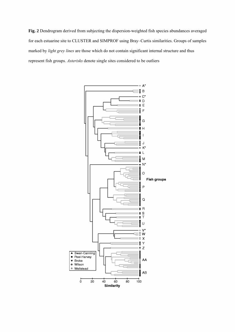
Fig. 2 Dendrogram derived from subjecting the dispersion-weighted fish species abundances averaged

for each estuarine site to CLUSTER and SIMPROF using Bray–Curtis similarities. Groups of samples

marked by light grey lines are those which do not contain significant internal structure and thus

represent fish groups. Asterisks denote single sites considered to be outliers

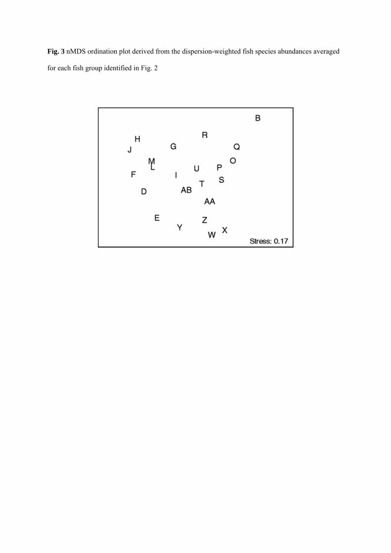
Fig. 3 nMDS ordination plot derived from the dispersion-weighted fish species abundances averaged

for each fish group identified in Fig. 2

Fig. 4 nMDS ordination plot derived from the dispersion-weighted fish species abundances averaged

for each fish group, with the sample scores for principal components (PC) 1 and/or 2 (derived from a

PCA of an environmental layer of interest) overlaid as circles of proportionate sizes. The only

exception is d, in which the circles represent the original data for the marine/freshwater

ratio. PO permanently-open, SO seasonally-open, NC normally-closed, SV submerged

vegetation, S’phire samphire, sg seagrass, ma macroalgae

Fig. 5 Shade plot illustrating the dispersion-weighted abundances of the most prevalent fish species in

each fish group (i.e. those species accounting for >5 % of the average abundance in at least one

group) with shading intensity being proportional to abundance. Fish groups are ordered by region

(and, within each region by their Bray–Curtis similarity) and species are ordered by a hierarchical

cluster analysis of their mutual associations across fish groups. The estuarine usage functional guild

for each species (sensu Potter et al. 2013) is given in superscript text (MS marine

straggler, MEO marine estuarine-opportunist, E solely estuarine, EM estuarine and

marine, EF estuarine and freshwater, FEO freshwater estuarine-opportunist)

Fig. 6 Linkage tree constructed using the dispersion-weighted and averaged fish species abundances

in each fish group as the reference, and the measurements for environmental attributes across all

scales as the explanatory data. The path to any fish group (terminal nodes of the tree) is determined by

the environmental thresholds given at each branching node, with unbracketed and bracketed

thresholds indicating a left and right path, respectively (N.B. threshold values have not been subjected

to any data pre-treatment). The units of measurement for each environmental attribute are given in the

‘Data for environmental layers’ subsection of the Methods and their abbreviations are as

follows: W west, S south, PO permanently-open, NC normally-closed, SO seasonally-open, M/F

ratio marine/freshwater ratio, Dist. wave shoal distance to wave shoaling margin, SV submerged

vegetation. E refers to exponential and B % reflects the magnitude of fish group differences as a

proportion of the maximum (measured by rank dissimilarities) at the initial division

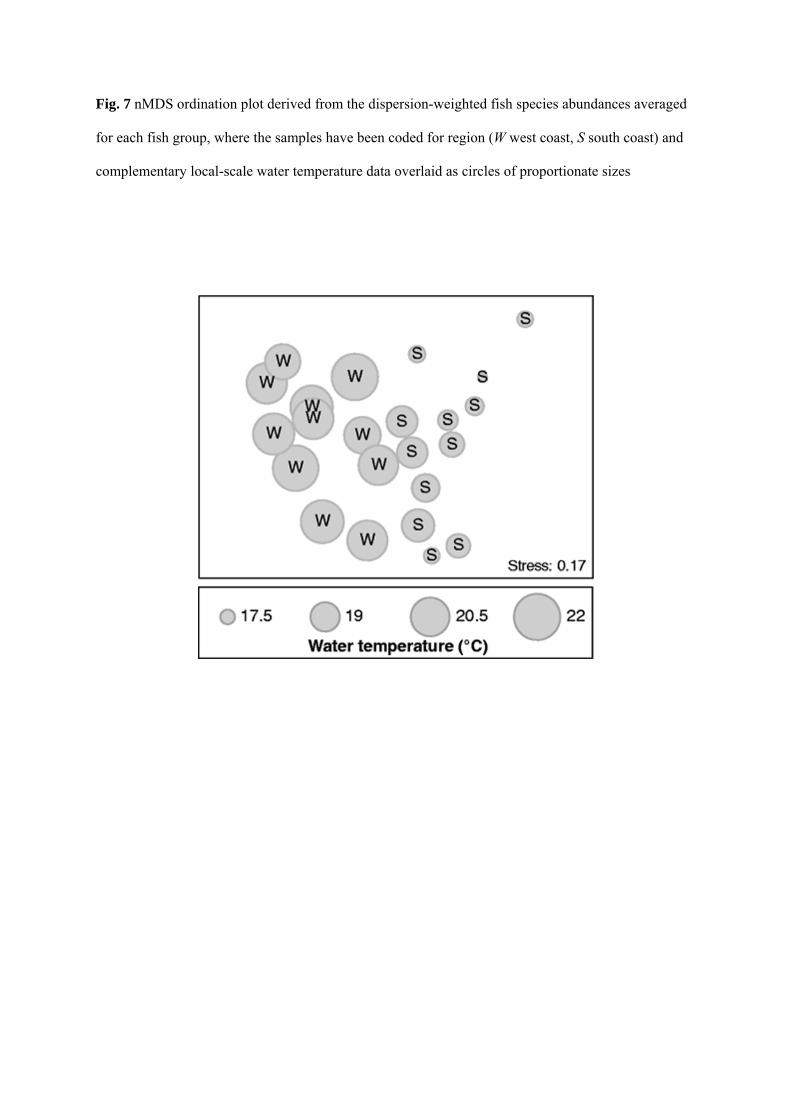
Fig. 7 nMDS ordination plot derived from the dispersion-weighted fish species abundances averaged

for each fish group, where the samples have been coded for region (W west coast, S south coast) and

complementary local-scale water temperature data overlaid as circles of proportionate sizes

Appendix

Table 2

Mean density (number of fish 100 m−2) and standard deviation (given in superscript values) of each fish species in each fish group (B–AB) identified in the Swan–Canning and Peel–Harvey estuaries (located on the west coast) and the Broke, Wilson and Wellstead estuarine systems (located on the south coast) in south-western Australia. Fish groups are ordered by region and, within each region, by their Bray–Curtis similarities. The estuarine usage functional guild for each species (sensu Potter et al. 2013) in south-western Australia is given after each species name, i.e. marine category (MS marine straggler, MEO marine estuarine-opportunist), estuarine category (E solely estuarine, EM estuarine and marine, EF estuarine and freshwater), diadromous category (SA semi-anadromous), freshwater category (FS freshwater straggler, FEO freshwater estuarine-opportunist)

West coast South coast

Y E D F J H M L G I AB U R T P O S Q AA Z X W B

Apogonidae

Ostorhinchus rueppellii EM 0.070.12 0.560.74 14.4827.30 1.630.75 3.853.80 4.013.72 6.686.60 0.210.37 1.652.15 6.617.26

Siphamia cephalotes MS 0.010.02 0.040.05 0.020.03

Arripidae

Arripis georgianus MEO 0.020.02 1.041.27 0.020.03

Arripis truttacea MS 0.040.05 0.040.05 0.020.03 <0.010.01

Atherinidae

Atherinomorus vaigiensis MEO 0.270.44 9.914.67 12.5010.11 15.7327.74 50.8244.62 16.7115.65 0.991.14 10.423.10 4.1010.05 0.420.98 0.750.84 0.190.46

Atherinosoma elongata E 0.180.28 0.110.15 1.191.63 1.882.49 0.040.07 0.070.10 19.2920.69 44.5462.58 54.8655.13 180.3572.96 228.85104.07 123.9852.16 23.098.50 137.0235.35 56.6031.69 31.529.69 198.24113.48 34.5119.94 336.17214.78 304.9717.14 1,186.48215.31 1,851.0433.11 7.970.53

Craterocephalus mugiloides E

11.2611.97 1.920.18 37.121.65 48.0117.46 0.030.04 23.3418.08 1.291.78 11.567.24 6.0714.15 0.080.07 3.348.18

Craterocephalus pauciradiatus E

0.520.74 1.301.82 13.8819.63 7.195.52 29.5633.43 12.615.13 0.210.51

Leptatherina presbyteroides EM 0.200.23 8.267.26 29.1421.83 160.09162.91 34.931.70 46.8845.28 31.0523.34 18.7712.09 17.4423.35 11.3012.14 76.3629.56 64.1936.07 111.82102.61 9.326.01 3.072.96 0.700.33 1.541.56 4.664.73 7.6710.24 0.140.15

Leptatherina wallacei EF 111.8029.38 27.6031.37 7.720.56 7.236.50 0.340.60 1.592.99 2.513.51 3.754.29 30.9639.70 22.1817.31 42.8112.12 14.745.07 134.3445.46 23.119.64 16.885.31 28.546.53 14.634.68 107.9664.75 324.55369.43 329.71283.66 74.5531.82 4.950.37

Blenniidae

Omobranchus germaini MS 0.020.03 0.010.02

Parablennius tasmanianus MS 0.080.22

West coast South coast

Y E D F J H M L G I AB U R T P O S Q AA Z X W B

Petroscirtes breviceps MS 0.040.05

Petroscirtes mitratus MS 0.010.02

Bothidae

Pseudorhombus jenynsii MEO 0.020.03 0.020.04 0.070.08 0.180.06 0.120.09 0.160.03 0.080.09 0.110.10 0.060.02 0.020.03 0.020.03

Callionymidae

Eocallionymus papilio MS 0.010.02

Carangidae

Pseudocaranx dentex MS 0.220.30 0.010.02 <0.010.02

Pseudocaranx wrighti MS 0.070.10

Clinidae

Cristiceps australis MS 0.020.02 0.060.08 0.020.03 0.050.08

Clupeidae

Hyperlophus vittatus MEO 0.020.04 0.250.25 0.090.08 0.230.29 276.49193.16 117.20255.47 35.3149.93 2.705.73 45.28119.58 237.88187.00 0.160.39

Nematalosa vlaminghi SA 1.901.79 1.851.19 0.320.15 0.050.07 0.150.34

Spratelloides robustus MEO 23.4636.85 7.108.35 0.771.04 0.350.91 0.160.42 10.2622.91

Cynoglossidae

Cynoglossus broadhursti MS 0.010.02

Engraulididae

Engraulis australis EM 2.774.76 0.360.46 0.040.09 0.010.02 <0.010.01 0.030.04 0.010.02 0.150.21 0.520.73 0.180.54 <0.010.02 0.080.13 0.360.20 0.110.15

Enoplosidae

Enoplosus armatus MS 0.040.09 0.060.08 0.010.02 0.310.33 0.010.03 0.030.05 0.020.03 0.020.03 <0.010.02

Galaxiidae

Galaxias occidentalis FS 0.130.20 0.010.03 0.050.12 <0.01

0.01

Gerreidae

Gerres subfasciatus MEO 0.010.02 0.200.13 0.180.10 0.170.30 0.010.02 0.180.01 0.010.02 0.030.05 0.230.56 1.380.84

Gobiidae

Afurcagobius suppositus EF 3.313.41 3.861.40 1.422.01 0.140.15 0.010.02 0.471.01 0.250.36 <0.010.01 0.300.46 4.873.92 3.011.74 0.700.69 9.000.08 8.252.96 4.211.35 1.380.43 0.860.68 4.225.59 8.9412.65 0.050.04

Arenigobius bifrenatus EM 5.108.84 0.340.48 0.050.11 0.090.13 0.050.11 0.680.97 <0.010.01 0.010.01 0.110.07 <0.010.02 0.130.13

Favonigobius lateralis EM 0.170.29 0.160.23 4.760.58 0.920.57 18.257.96 6.098.20 17.102.37 30.233.78 1.571.60 23.815.42 0.831.34 4.121.72 0.250.20 5.016.39 0.610.69 0.490.58 2.102.06 0.490.52 4.224.27 2.622.84 1.290.86 52.638.52 0.060.02

Favonigobius punctatus E 2.832.01 17.0614.17 9.552.34 2.171.65 0.100.10 0.130.13 3.843.01 1.260.97 0.932.26 5.174.27 2.322.02

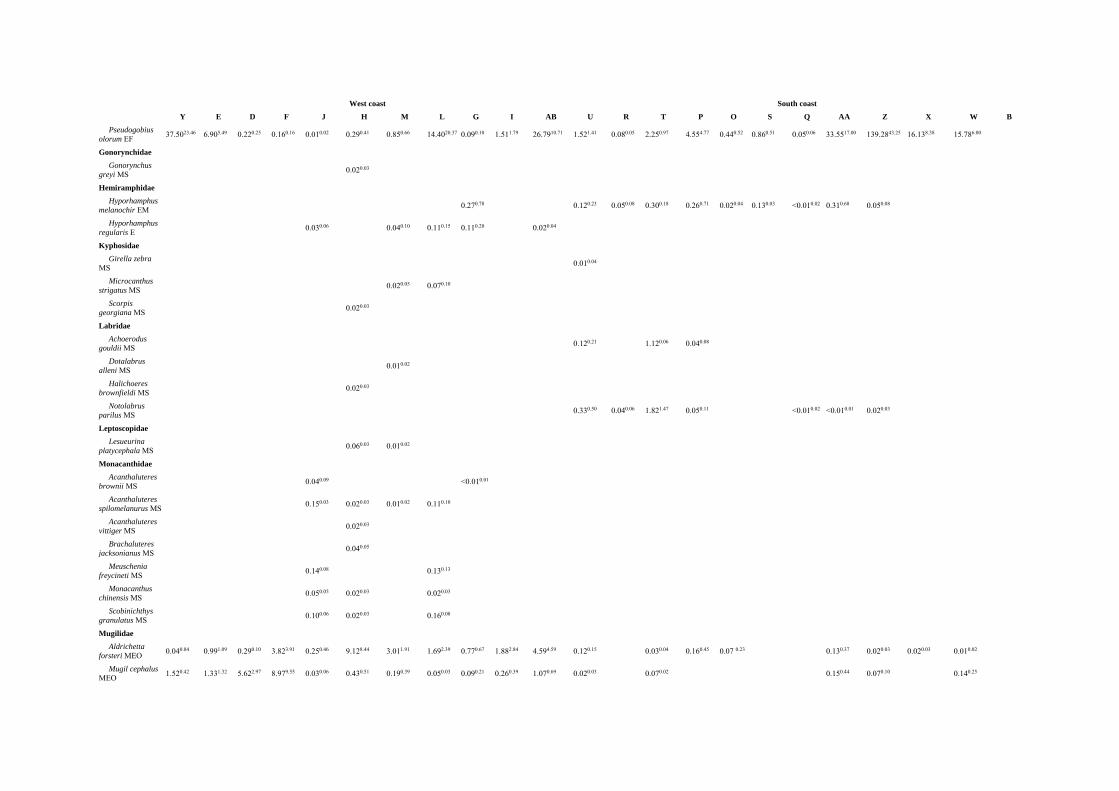
West coast South coast

Y E D F J H M L G I AB U R T P O S Q AA Z X W B

Pseudogobius olorum EF 37.5023.46 6.905.49 0.220.25 0.160.16 0.010.02 0.290.41 0.850.66 14.4020.37 0.090.10 1.511.79 26.7910.71 1.521.41 0.080.05 2.250.97 4.554.77 0.440.52 0.860.51 0.050.06 33.5517.00 139.2843.25 16.138.38 15.786.00

Gonorynchidae

Gonorynchus greyi MS 0.020.03

Hemiramphidae

Hyporhamphus melanochir EM 0.270.78 0.120.23 0.050.08 0.300.18 0.260.71 0.020.04 0.130.03 <0.010.02 0.310.68 0.050.08

Hyporhamphus regularis E 0.030.06 0.040.10 0.110.15 0.110.20 0.020.04

Kyphosidae

Girella zebra MS 0.010.04

Microcanthus strigatus MS 0.020.05 0.070.10

Scorpis georgiana MS 0.020.03

Labridae

Achoerodus gouldii MS 0.120.21 1.120.06 0.040.08

Dotalabrus alleni MS 0.010.02

Halichoeres brownfieldi MS 0.020.03

Notolabrus parilus MS 0.330.50 0.040.06 1.821.47 0.050.11 <0.010.02 <0.010.01 0.020.03

Leptoscopidae

Lesueurina platycephala MS 0.060.03 0.010.02

Monacanthidae

Acanthaluteres brownii MS 0.040.09 <0.010.01

Acanthaluteres spilomelanurus MS 0.150.03 0.020.03 0.010.02 0.110.10

Acanthaluteres vittiger MS 0.020.03

Brachaluteres jacksonianus MS 0.040.05

Meuschenia freycineti MS 0.140.08 0.130.13

Monacanthus chinensis MS 0.050.05 0.020.03 0.020.03

Scobinichthys granulatus MS 0.100.06 0.020.03 0.160.08

Mugilidae

Aldrichetta forsteri MEO 0.040.04 0.991.09 0.290.10 3.823.91 0.250.46 9.128.44 3.011.91 1.692.39 0.770.67 1.882.84 4.594.59 0.120.15 0.030.04 0.160.45 0.07 0.23 0.130.37 0.020.03 0.020.03 0.010.02

Mugil cephalus MEO 1.520.42 1.331.32 5.622.97 8.979.55 0.030.06 0.430.51 0.190.39 0.050.03 0.090.21 0.260.39 1.070.69 0.020.03 0.070.02 0.150.44 0.070.10 0.140.25

West coast South coast

Y E D F J H M L G I AB U R T P O S Q AA Z X W B

Mullidae

Upeneus tragula MS 0.020.03

Odacidae

Haletta semifasciata MS 0.840.75 0.440.19 0.070.09 2.070.94 0.010.02 0.010.04 0.020.04

Neoodax balteatus MS 0.280.22 0.010.02 0.040 0.020.03 0.240.34 0.010.02

Siphonognathus radiatus MS 0.020.02

Percichthyidae

Edelia vittata FS 0.010.02

Pinguipedidae

Parapercis haackei MS 0.010.02 0.020.03

Platycephalidae

Platycephalus endrachtensis E 0.080.11 0.020.03 0.040.05 0.050.05 0.030.02 0.060.07 0.020.06

Platycephalus fuscus MS <0.010.01

Platycephalus laevigatus MS 0.010.02 0.040.05

Platycephalus speculator EM 0.010.02 0.040.05 0.040.05 0.010.03 0.010.01 0.020.04 0.040.05

Pleuronectidae

Ammotretis elongatus MEO 0.070.14 1.300.19 0.330.39 0.100.15 0.230.26 0.020.04 0.030.03 0.150.21

Ammotretis rostratus MEO 0.010.03 0.170.21 0.060.09 0.050.01 0.010.02 0.010.02 0.010.03 <0.010.01 0.020.03

Plotosidae

Cnidoglanis macrocephalus EM 0.010.02 0.020.03 0.040 0.060.17

Poeciliidae

Gambusia affinis FEO 4.327.46 0.050.08 0.020.03 0.480.86 0.010.03

Sillaginidae

Sillaginodes punctatus MEO 0.070.05 0.030.02 0.050.08 0.140.20 0.200.23 0.450.94 0.260.35 0.020.04 0.040.11 0.020.06 0.050.08

Sillago bassensis MS <0.010.01

Sillago burrus MEO 0.040.05 0.240.25 1.140.77 0.390.69 0.140.15 0.060.09 0.370.66 0.020.02

Sillago schomburgkii MEO

0.030.03 0.110.22 0.470.61 0.190.17 0.220.20 0.310.64 0.210.46 0.040.06

Sillago vittata MEO 0.120.21 0.060.03 0.010.02 0.010.02

Sparidae

West coast South coast

Y E D F J H M L G I AB U R T P O S Q AA Z X W B

Acanthopagrus butcheri E 14.474.43 23.424.32 12.251.22 6.495.18 0.310.63 0.060.02 0.290.36 0.160.36 0.440.63 0.640.43 0.210.62 5.898.33 0.810.94 0.120.11

Rhabdosargus sarba MEO 0.020.03 0.060.13 0.110.05 0.040.08 0.210.37 0.090.19 0.020.03

Syngnathidae

Filicampus tigris MS 0.010.02 0.020.03

Pugnaso curtirostris MS 0.080.10 0.020.03 0.060.11 0.020.03

Stigmatopora argus MS 2.681.05 3.644.04 0.190.37 2.050.25 0.030.08

Urocampus carinirostris EM 0.030.03 0.040.07 0.020.03 0.020.03 0.400.41 0.020.04 0.090.13 0.030.02 0.010.02 0.050.08 0.150.27 0.130.18

Terapontidae

Amniataba caudavittata E 3.142.45 10.632.69 5.240.05 1.941.19 0.901.27 0.020.03 0.040.09 0.010.02 0.250.32

Pelates octolineatus MEO 2.281.09 0.050.08 0.310.30 1.812.60 0.450.32 6.3810.49 9.210.28 0.440.85 0.550.87 2.894.63 0.020.03

Tetraodontidae

Contusus brevicaudus MS 0.050.02 0.040.06 0.050.08 0.010.02 0.020.03 0.010.02

Polyspina piosae MS 0.480.97

Torquigener pleurogramma MEO

0.030.05 2.683.73 20.220.86 27.5010.69 61.2420.65 8.633.11 19.476.13 20.991.75 9.184.22 2.422.57 6.464.78 0.270.67

Tetrarogidae

Gymnapistes marmoratus MEO 0.030.03 0.440.29 0.640.05 0.530.95 1.111.12 0.030.06 0.130.21 0.010.02 0.020.03 0.020.03 0.070.10

Number of species 22 25 21 29 47 46 45 47 40 36 34 28 11 16 16 12 10 10 20 21 8 10 5

Total mean density 201 113 127 170 325 375 269 233 118 350 584 257 104 404 103 57 232 52 492 795 1,535 1,994 13