Research on real -time elimination of UWB radar ranging ...

1

Research on real-time elimination of UWB radar ranging abnormal

value data

Xin Yan, Hui Liu, Guoxuan Xin, Hanbo Huang, Yuxi Jiang, Ziye Guo

School of Electrical and Information Engineering, Beijing University of Civil Engineering and Architecture. Beijing 100044,

China 5

Correspondence to: Xin Yan([email protected])

Abstract. For indoor positioning, ultra-wideband (UWB) radar comes to the forefront due to its strong penetration, anti-

jamming, and high precision ranging abilities. However, due to the complex indoor environment and disorder of obstacles,

the problems of diffraction, penetration, and ranging instability caused by UWB radar signals also emerge. During the

experiment of indoor positioning with UWB radar ranging module P440, it was found that the distance information 10

measured in a short time was unstable, because of the complex indoor environment and unpredictable noise signal. Therefore,

the abnormal value migration of the positioning trajectory occurred in real-time positioning. To eliminate this phenomenon

and provide more accurate results, the abnormal values need to be removed. It is not difficult to eliminate abnormal value

accurately based on a large number of data, but it is still a difficult problem to ensure the stability of the positioning system

by using a small amount of measurement data in a short time to eliminate abnormal value in real-time ranging data. Thus, 15

this paper focuses on the experimental analysis of a UWB-based indoor positioning system. To improve the stability of

UWB radar ranging data and increase the overall accuracy, this paper studies a large number of UWB radar ranging data by

using high-frequency ranging instead of mean value to train estimation model. Based on the Gaussian function outlier

detection, abnormal values are eliminated. By using the training distance estimation model and estimating the distance value,

the ranging error obtained is nearly 50% lower than the peak and mean ranging errors in general. 20

1 Introduction

UWB technology, due to its high transmission rate, penetration, security, and low system complexity, has been favored by

many scholars in the field of indoor positioning. In 2014, Khajenasiri et al. (2014) developed a low power UWB transceiver

for smart home energy consumption monitoring and management, which is one order lower than the commercial wireless

technology applied in smart home applications. In 2017, Mokhtari et al. (2017) put forward the use of UWB technology to 25

monitor some high-risk areas in a smart home environment. In 2012, Madany et al. (2012) investigated ITS and proposed the

use of UWB technology in vehicle-to-vehicle and vehicle-to-infrastructure communication of multi-user ITS technology. In

2018, Mostajeran et al. (2018) proposed a UWB full-scale imaging radar with Asia-Pacific Hertz frequency. This was the

https://doi.org/10.5194/gi-2019-42Preprint. Discussion started: 22 June 2020c© Author(s) 2020. CC BY 4.0 License.

2

first THz/sub-THz frequency imaging radar providing good lateral resolution without any focal lens or reflector. For objects

with a distance of 23cm, it achieved 2mm lateral resolution and 2.7mm range resolution. 30

In 2016, Kim and Choi (2016) proposed an automatic landing system for UAS based on the UWB, optimized the geometric

structure of the UWB anchor in the network, and achieved a more accurate positioning performance for the UAS landing

process. In 2018, Nakamura et al. (2018) studied a pedestrian positioning system based on UWB ranging. In this system, the

base station receiving the UWB signals transmitted by the pedestrians was connected to the traffic lights, and the locations of

pedestrians was estimated by the least square method using the distance estimated by the UWB ranging scheme. In 2017, 35

Kolakowski (2017) proposed the concept combining Bluetooth low power (BLE) and UWB positioning to improve the

energy efficiency. In 2017, Ruiz et al. (2017) compared the performance of three commercial UWB systems, namely

Ubisense, BeSpoon, and DecaWave, under the same experimental conditions. A measurement model combining Bayesian

and particle filters was used. The model considered errors in distance measurement and found the abnormal values. The

results indicated which system performed better under these industrial conditions. In 2015, Ledergerber et al. (2015) 40

proposed a self-positioning robot system based on one-way UWB communication. By passively receiving the UWB radio

signals from a fixed position, the position of the robot in a certain space was estimated. In 2016, Hepp et al. (2016) proposed

an omnidirectional tracking system for flying robots based on blocking robust UWB signals. Compared to the typical UWB

positioning systems with a fixed UWB converter in the environment, this system only needed one UWB converter to detect

the target. In 2017, Perez-Grau et al. (2017) proposed a multi-modal mapping system based on UWB and RGB-D. By using 45

the synergy between the UWB sensor and point cloud, a multi-mode three-dimensional (3D) map with a UWB sensor was

generated for location estimation, which was integrated into the Monte Carlo localization method. In 2018, Schroeer (2018)

used a real-time UWB multi-channel indoor positioning system for industrial scenes to evaluate multi-path and non-line-of-

sight situations. In the same year, Stampa et al. (2018) proposed a semi-automatic calibration method for the UWB-based

distance measurement of the autonomous mobile robots. Aiming at the system ranging error observed in the UWB distance 50

measurement, a semi-automatic calibration method was proposed to estimate the error model approximating its influence.

The research on UWB in China, however, started relatively late. Although it is not as mature as that of foreign countries,

some works have been done with the strong support of the state. In 2010, Chen et al. (2010) designed a UWB transmitter

combined with a digital pulse generator and a modulator to minimize the power consumption. In 2015, Wang et al. (2015)

proposed the use of UWB technology to monitor the load in football training. In 2016, Zhang et al. (2016) used UWB radar 55

to image two targets behind the double-wall using the time-domain back projection (BP) and the frequency domain phase

shift (PSM) algorithms. In 2017, Ke et al. (2017) proposed an integrated method of intelligent vehicle navigation and

positioning based on GPS and UWB. When a vehicle was in a position where the GPS signals were difficult to receive, such

as tunnels, the positioning was fulfilled by UWB, and the lost GPS signals were used to replace the integrated positioning of

the vehicles. In 2016, Dai et al. (2016) analyzed the main factors affecting the UWB positioning accuracy in a hazardous 60

chemicals warehouse and accordingly proposed a UWB four-reference vector compensation method for the stacking location,


3

which was suitable for monitoring the five-segment distance. In 2017, Fu et al. (2017) proposed a method to detect the

attitude of the road header by using the UWB ranging technology to realize the unmanned driving.

UWB radar is favored by researchers of indoor positioning systems because of its strong penetration, anti-jamming, and high

precision ranging ability. However, due to the complex indoor environment and the disorder of obstacles, the problem of 65

diffraction, penetration, and ranging instability of UWB radar signals also emerge. Thus, this paper focuses on the

experimental analysis of a UWB-based indoor positioning system. To , the stability and accuracy of UWB radar ranging data

are further improved. Aiming at the real-time measurement of a large amount of UWB radar ranging data, this paper

proposes that the processing of the acquired data has to be performed immediately to meet the real-time requirement of the

positioning systems. Thus, abnormal values and redundant data in ranging can be removed in real-time, and more accurate 70

and stable results can be delivered to an indoor positioning module.

that the range information measured in a short time is very unstable and even has abnormal values due to the complex indoor

environment and unpredictable noise signals. The abnormal values should be eliminated. Based on this, this paper focuses on

the experimental analysis of a UWB radar indoor positioning system. To improve the stability of UWB radar ranging data

and increase the overall accuracy, this paper studies a large number of UWB radar ranging data by using high-frequency 75

ranging instead of mean value to train estimation model. The high-frequency range value is used instead of the mean value,

and the distance estimation model is trained. The abnormal value is detected based on the function, and the abnormal value is

removed after training. The ranging error obtained by distance measurement is nearly 50% lower than that of peak and mean

ranging errors.

2 P440 UWB wireless sensor location framework 80

The P440 UWB wireless sensor operates at a center frequency of 4.3 GHz and has a bandwidth of 2.2 GHz. The signal

ranging accuracy of ideal laboratory environment calibration can reach 0.05 m and works well in extremely challenging

environments. The testbed for positioning in laboratory using the P440 UWB wireless sensor is shown in Fig. 1.

This experiment is used to realize indoor 3D positioning. Four P440 UWB wireless sensors are used as base stations (also

called anchor nodes), and a P440 UWB wireless sensor is used as a node to be tested, which can be installed in mobile 85

devices usually used in indoors (e.g., sports robots). The P440 can obtain the distance information between two nodes. By

using this and the positioning algorithm, the t coordinates of each node in 3D can be acquired, and the three-dimensional

positioning result of the node to be tested can be obtained.

The experimental results of the 3D positioning in a laboratory environment are shown in Fig. 2. It is found that, due to the

complex indoor environment, the interference from indoor objects is relatively serious, resulting in unstable distance 90

information measured in a short period of time, and even abnormal values. Therefore, when performing real-time positioning,

the positioning trajectory generates an abnormal value offset phenomenon. In order to improve the stability and accuracy of


4

the real-time positioning, the original ranging data need to be analysed and processed as reducing the influence of the

abnormal values, so that the target point to be tested is stabilized in a small range.

3 Ranging data analysis 95

3.1 Distribution function and parameter estimation of the ranging data

In the laboratory environment, two P440 wireless sensors were used to obtain a large amount of ranging data from four

different distance locations, and Fig. 3 shows the histogram of the data acquired. As seen, the data obtained follows a Gauss

distribution, which can be formulated as

𝑓(𝑥) =1

√2𝜋𝜎𝑒𝑥𝑝 [−

(𝑥−𝜇)2

2𝜎2] (1) 100

The laboratory fits its probability density distribution curve for these four sets of data, as shown in Fig. 4. As seen, the

expected value deviates from the true value, i.e., there is a huge difference in the standard deviation of the Gaussian

distribution for each group of data. Table 1 gives the expected and standard deviation of the estimated four sets of data. This

is an indicator of abnormal values, which causes measurement discrepancy between the measurements and the true values.

Thus, the data cannot be used for positioning due to the abnormal values. 105

3.2 Mean, peak, and true values of the ranging data

In the above-given measurement data, due to the disturbance of abnormal values, the deviation between the expected, peak,

and the true values are high. In positioning, especially for mobile tracking, it is impossible to collect a large amount of data

in a short time. Therefore, we collected only 60 groups of measurement data from different distances and accordingly

calculated their mean and peak values. 110

3.3 Distance estimation model training

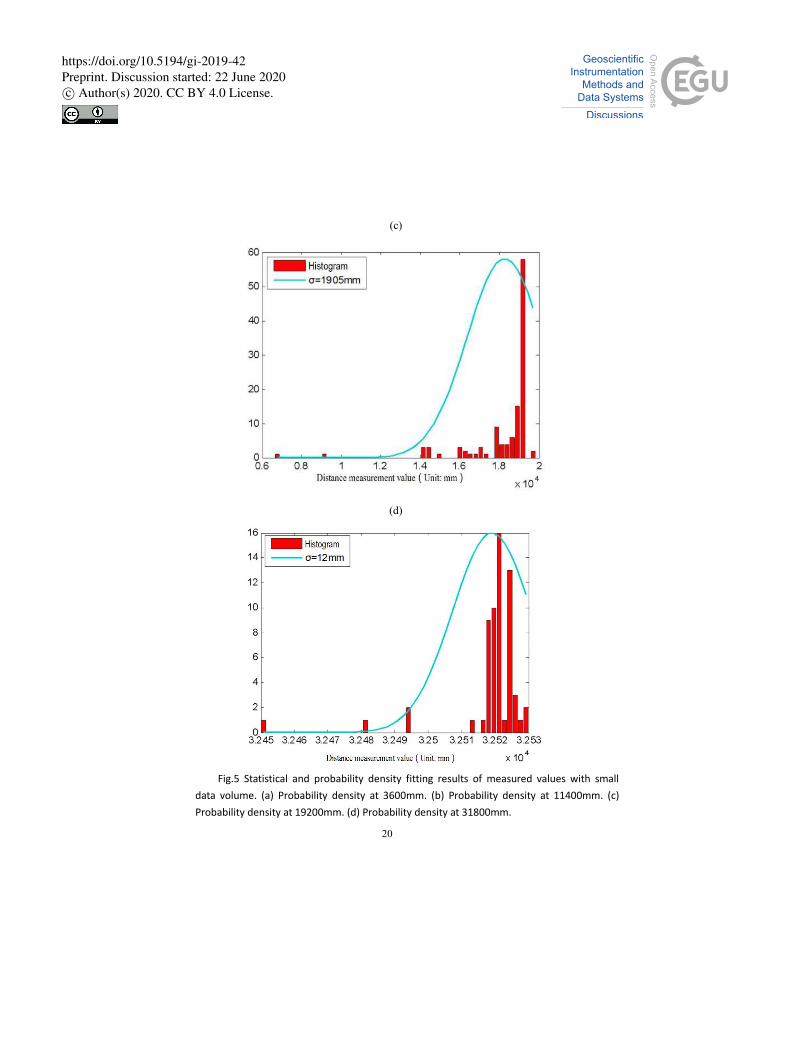
Figure 5 and Table 2 show that using the mean peak as a reference, though and there is certain error between the true value,

but it can be seen that the distance between true value and measure the peak of a certain linear relationship will be measured,

as shown in Fig. 6 (scattered dots in red). By using a polynomial, 50 of the 60 sets of data were selected as the training set to

fit the linear relationship between the peak and the true values of the measured data, as shown by the solid cyan line in Fig. 6. 115

The other 10 sets are set aside as test sets. Table 2 shows the statistical results of the true, peak, and mean values of the

selected 50 groups of data.


5

4 Data processing methods

The statistical results of the peak and true values in Section 3 showed that the deviation between the peak and the true values

is linear, satisfying a certain relationship. Since the ranging data follows a Gaussian distribution, the peak value is taken as 120

the reference mean for processing. Then, the ranging results that the reference mean meets certain conditions are retained,

and those that do not meet the conditions, i.e., abnormal values are removed. Finally, the true value of the distance is

estimated for normal data according to the fitted curve in Fig. 6 reducing the ranging error. By using linear fitting, the

relationship between the peak and true values can be formulated as

𝑦 = 0.9859𝑥 − 0.1633, (2) 125

where 𝑥 is the peak value, and 𝑦 is the true.

4.1 Gaussian abnormal value detection

Since the distance measurement follows a Gaussian distribution 𝑁~(𝜇, 𝜎2), the Gaussian function is used for abnormal

value detection. Here, the abnormal values and the normal data are calibrated, the abnormal value data is eliminated, and the

normal data is retained. 130

𝑥 = (𝑦 + 0.1633)/0.9859. (3)

Since the measurement data satisfies the Gaussian distribution 𝑁~(𝜇, 𝜎2), it is known from (3) that when the distance

estimation is carried out by (2), the estimated value also satisfies the Gaussian distribution. The estimated mean 𝜇𝑦 the and

standard deviation 𝜎𝑦 can be expressed as

𝜇𝑦 = 0.9859𝜇 − 0.1633, (4) 135

𝜎𝑦 = 0.9859𝜎. (5)

Therefore, if it is desired to obtain an estimated value error less than 𝛿𝑦, the error 𝑥 between the measured value of 𝛿𝑥 and

the peak value has to satisfy 𝛿𝑥 < 𝛿𝑦/0.9859.

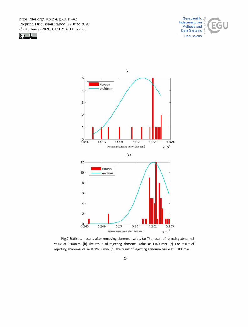
According to this method, abnormal values were detected for the four groups of data, and the results were shown in Fig. 7.

As seen, the method successfully removes the abnormal values. Among the four groups of data, the first three groups had a 140

very large standard deviation due to the existence of abnormal value. After the elimination of abnormal value, the standard

deviation remained within 50mm.

4.2 Estimating the truth value

After removing the abnormal value by the Gaussian function, according to the above analysis, the ranging value cannot be

directly used for positioning. This is because the error between the ranging peak and the true values of the P440 is still high, 145


6

and thus the required ranging value needs to be retained. The estimation is performed by using (2), and the results are shown

in Table 3, which gives the estimated values of the 10 sets of test data. Table 4, on the other hand, shows the overall error

when estimating the ranging distance by using peaks, expected values, and the methods proposed in this paper.

5 Conclusion

In this paper, the experimental analysis and research on the ranging data of the UWB radar indoor positioning system were 150

carried out. To meet the needs of indoor real-time positioning, further improve the stability of UWB radar ranging data and

the overall accuracy, a large amount of UWB radar ranging data were studied, and the high-frequency ranging value was

used to replace the mean value and train the range estimation model. The abnormal value was detected based on the

Gaussian function. After removing the abnormal value, the distance estimation model was used to estimate the distance

value. The results showed that the distance measurement error obtained is nearly 50% lower than the peak and mean distance 155

measurement errors.

Author contribution

Xin Yan and BB designed the experiments and Xin Yan developed the model code. Xin Yan, Guoxuan Xin and Hanbo

Huang carried them out. Xin Yan prepared the manuscript with contributions from all co-authors. Hui Liu, Yuxi Jiang and

Ziye Guo revised the manuscript. 160

Competing interests

The authors declare that they have no conflict of interest.

Funding

Name of Funder: National Natural Science Foundation of China

Grant Agreement No.: 61501019 165

Name of Funder: Scientific Research Project of Beijing Educational Committee

Grant Agreement No.: SQKM201710016008

Name of Funder: The Fundamental Research Funds for Beijing University of Civil Engineering and Architecture

Grant Agreement No.: 18209

170


7

References

Chen, F. H., Lin, S. Y., Li, L. Y., Sun, X. W.: 4.2-4.8 GHz CMOS variable gain LNA for Chinese UWB application, in:

2010 International Conference on Microwave and Millimeter Wave Technology, Chengdu, China, 8-11 May 2010,

1922-1924, 2010.

Dai, B., Lv, X., Liu, X. J., Li, Z. C.: A UWB-based four reference vectors compensation method applied on hazardous 175

chemicals warehouse stacking positioning, CIESC J., 67, 871-877, 2016.

Fu, S., Li, Y., Zong, K., Zhang, M., Wu, M.: Accuracy analysis of UWB pose detection system for roadheader, Chin. J. Sci.

Instrum., (8), 17, 2017. (in Chinese)

Hepp, B., Nägeli, T., Hilliges, O.: Omni-directional person tracking on a flying robot using occlusion-robust ultra-wideband

signals, in: 2016 IEEE/RSJ International Conference on Intelligent Robots and Systems (IROS), Daejeon, South Korea, 180

9-14 October 2016, 189-194, 2016.

Ke, M., Zhu, B., Zhao, J., Deng, W.: Integrated positioning method for intelligent vehicle based on GPS and UWB, SAE Int.

J. Passeng. Cars – Electron. Electr. Syst., 11, 40-47, https://doi.org/10.4271/07-11-01-0004, 2017.

Khajenasiri, I., Zhu, P., Verhelst, M., Gielen, G.: Low-energy UWB transceiver implementation for smart home energy

management, in: The 18th IEEE International Symposium on Consumer Electronics (ISCE 2014), JeJu Island, South 185

Korea, 22-25 June 2014, 1-2, 2014

Kim, E., Choi, D.: A UWB positioning network enabling unmanned aircraft systems auto land, Aerosp. Sci. Technol., 58,

418-426, https://doi.org/10.1016/j.ast.2016.09.005, 2016.

Kolakowski, M.: Kalman filter based localization in hybrid BLE-UWB positioning system, in: 2017 IEEE International

Conference on RFID Technology & Application (RFID-TA), Warsaw, Poland, 20-22 September 2017, 290-293, 2017. 190

Ledergerber, A., Hamer, M., D'Andrea, R.: A robot self-localization system using one-way ultra-wideband communication,

in: 2015 IEEE/RSJ International Conference on Intelligent Robots and Systems (IROS), Hamburg, Germany, 28

September-2 October 2015, 3131-3137, 2015

Madany, Y. M., Elaziz, D. A., Elkrim, W. A.: Design and analyis of compact ultra-wideband inverted FL microstrip patch

antenna for intelligent transportation communication systems, in: 2012 15 International Symposium on Antenna 195

Technology and Applied Electromagnetics, Toulouse, France, 25-28 June 2012, 1-4, 2012.

Mokhtari, G., Zhang, Q., Fazlollahi, A.: Non-wearable UWB sensor to detect falls in smart home environment, in: 2017

IEEE International Conference on Pervasive Computing and Communications Workshops (PerCom Workshops), Kona,

HI, USA, 13-17 March 2017, 274-278, 2017.

Mostajeran, A., Naghavi, S. M., Emadi, M., Samala, S., Ginsburg, B. P., Aseeri, M., Afshari, E.: A high-resolution 220-GHz 200

ultra-wideband fully integrated ISAR imaging system, IEEE Trans. Microw. Theory Tech., 67, 429-442,

https://doi.org/10.1109/TMTT.2018.2874666, 2018.


8

Nakamura, A., Shimada, N., Itami, M.: Performance analysis of UWB positioning system at the crossing, in: 2018 21st

International Conference on Intelligent Transportation Systems (ITSC), Maui, HI, USA, 4-7 November. 2018, 786-791,

2018. 205

Perez-Grau, F. J., Caballero, F., Merino, L., Viguria, A.: Multi-modal mapping and localization of unmanned aerial robots

based on ultra-wideband and RGB-D sensing, in: 2017 IEEE/RSJ International Conference on Intelligent Robots and

Systems (IROS), Vancouver, BC, Canada, 24-28 September 2017, 3495-3502, 2017.

Ruiz, A. R., Granja, F. S.: Comparing Ubisense, BeSpoon, and DecaWave UWB location systems: Indoor performance

analysis, IEEE Trans. Instrum. Meas., 66, 2106-2117, https://doi.org/10.1109/TIM.2017.2681398, 2017. 210

Schroeer, G.: A real-time UWB multi-channel indoor positioning system for industrial scenarios, in: 2018 International

Conference on Indoor Positioning and Indoor Navigation (IPIN), Nantes, France, 24-27 September 2018, 1-5, 2018.

Stampa, M., Mueller, M., Hess, D., Roehrig, C.: Semi-automatic calibration of UWB range measurements for an

autonomous mobile robot, in: ISR 2018; 50th International Symposium on Robotics, Munich, Germany, 20-21 June

2018, 1-6, 2018. 215

Wang, K.: Application of UWB technology in the development of football training load monitoring system, Int. J. Simul.

Syst. Sci. Technol., 16, 8.1-8.6, https://doi.org/10.5013/IJSSST.a.16.3B.08, 2015.

Zhang, H., Zhang, Y., Wang, F.: UWB radar imaging of multiple targets through multi-layer walls, Int. J. Hybrid Inf.

Technol., 9, 315-322, https://doi.org/10.14257/ijhit.2016.9.8.27, 2016.

220


9

Table 1 Expectation and standard deviation of distance measurements.

Truth value (mm) Expectations value (mm) standard deviation (mm)

3560 3810 48.19

9640 9633 58.41

28220 28719 37.80

41540 41973 96.57


10

Table 2 Truth value, (measured) peak value, and (measured) mean value of the 50 training data sets.

Truth value (m) Peak value (m) Mean value (m)

0.6 0.707 0.705

1.2 1.25 1.247

1.8 1.892 1.894

2.4 2.512 2.5

3 3.085 3.098

3.6 3.723 3.588

4.8 4.882 4.892

5.4 5.492 5.332

6 6.118 5.852

6.6 6.684 6.88

7.2 8.514 8.368

7.8 7.911 7.317

8.4 8.461 8.543

9.6 10.514 9.741

10.2 11.061 10.851

10.8 10.851 10.415

11.4 13.219 12.007

12 12.403 12.401

12.6 13.468 12.954

13.2 13.32 13.241

13.8 13.999 13.878

15 15.417 14.658

15.6 16.025 16.043

16.2 16.474 15.667

16.8 16.773 16.155

17.4 17.4 17.009

18.6 18.862 18.009

19.2 19.274 18.271

19.8 20.396 19.315

21 20.97 20.375

21.6 21.706 21.139

22.2 22.389 21.625

23.4 23.377 22.867

24 24.557 24.095

24.6 25.134 24.818

25.2 25.894 25.648

25.8 26.512 26.484

26.4 27.172 27.147

27.6 28.258 28.243

28.2 28.738 28.719

28.8 29.507 29.473

29.4 29.924 29.938

30 30.473 30.247

31.2 31.9 31.897

31.8 32.522 32.519

32.4 33.116 33.097

33 33.705 33.693

34.2 34.889 34.884

34.8 35.477 35.472

36 36.634 36.568


11

Table 3 Results of true value estimation for 10 sets of test data. 225

Truth value (m) Peak value (m) Expectations value (m) Estimated value (m)

4.2 4.321 4.29 4.096774

9 9.01 8.318 8.719659

14.4 14.585 14.331 14.21605

18 17.989 17.576 17.57206

20.4 20.487 19.898 20.03483

22.8 23.593 23.197 23.09704

27 27.667 27.542 27.1136

30.6 31.152 31.149 30.54946

33.6 34.314 34.293 33.66687

35.4 36.039 36.044 35.36755


12

Table 4 Overall estimation error.

Peak estimation error (m) Expected estimation error (m) This method estimates the error (m)

0.3779 0.4592 0.1921


13

Figure captions

Figure 1 Framework of 3D indoor positioning system.

Figure 2 Schematic diagram of the target location results to be measured. 230

Figure 3 Histogram of the measured values at different distances. (a) Histogram of the measured value at 3560mm. (b) Histogram of the

measured value at 9640mm. (c) Histogram of the measured value at 28220mm. (d) Histogram of the measured value at 41540mm.

Figure 4 Fitting results of the probability density distribution curve. (a) Probability density at 3560mm. (b) Probability density at 9640mm.

(c) Probability density at 28200mm. (d) Probability density at 41540mm.

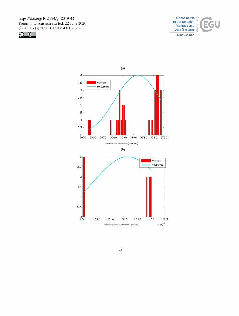
Figure 5 Statistical and probability density fitting results of measured values with small data volume. (a) Probability density at 3600mm. 235 (b) Probability density at 11400mm. (c) Probability density at 19200mm. (d) Probability density at 31800mm.

Figure 6 Statistical results and fitting of the peak and true values of distance measurement.

Figure 7 Statistical results after removing abnormal value. (a) The result of rejecting abnormal value at 3600mm. (b) The result of

rejecting abnormal value at 11400mm. (c) The result of rejecting abnormal value at 19200mm. (d) The result of rejecting abnormal value

at 31800mm. 240


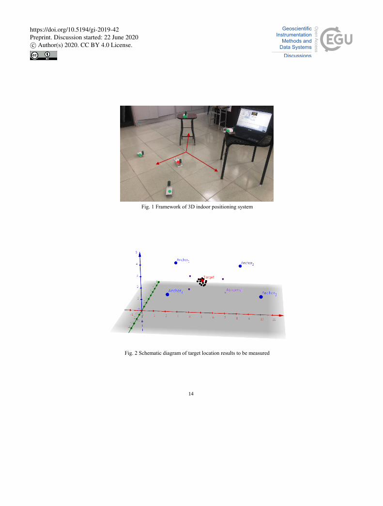
Fig. 1 Framework of 3D indoor positioning system

Fig. 2 Schematic diagram of target location results to be measured

14


(a)

(b)

15


(c)

(d)

Fig.3 Histogram of the measured values at different distances. (a) Histogram of the

measured value at 3560mm. (b) Histogram of the measured value at 9640mm. (c) Histogram

of the measured value at 28220mm. (d) Histogram of the measured value at 41540mm.

16


(a)

(b)

17


(c)

(d)

Fig.4 Fitting results of the probability density distribution curve. (a) Probability density

at 3560mm. (b) Probability density at 9640mm. (c) Probability density at 28200mm. (d)

Probability density at 41540mm.

18


(a)

(b)

19


(c)

(d)

Fig.5 Statistical and probability density fitting results of measured values with small

data volume. (a) Probability density at 3600mm. (b) Probability density at 11400mm. (c)

Probability density at 19200mm. (d) Probability density at 31800mm.

20


Fig.6 Statistical and fitting results of peak value and truth value of distance measurement

21


(a)

(b)

22


(c)

(d)

Fig.7 Statistical results after removing abnormal value. (a) The result of rejecting abnormal

value at 3600mm. (b) The result of rejecting abnormal value at 11400mm. (c) The result of

rejecting abnormal value at 19200mm. (d) The result of rejecting abnormal value at 31800mm.

23


Research on real -time elimination of UWB radar ranging ...

Documents