Research Article An Improved Performance Measurement Approach for Knowledge-Based Companies Using Kalman Filter Forecasting Method Mohammad Reza Hasanzadeh, Behrooz Arbab Shirani, and Gholam Ali Raissi Ardali Department of Industrial & Systems Engineering, Isfahan University of Technology, Isfahan, Iran Correspondence should be addressed to Mohammad Reza Hasanzadeh; [email protected] Received 3 July 2016; Accepted 25 August 2016 Academic Editor: Alessandro Lo Schiavo Copyright © 2016 Mohammad Reza Hasanzadeh et al. is is an open access article distributed under the Creative Commons Attribution License, which permits unrestricted use, distribution, and reproduction in any medium, provided the original work is properly cited. Performance measurement and forecasting are crucial for effective management of innovative projects in emerging knowledge- based companies. is study proposes an integrated performance assessment and forecasting model based on a combination of earned schedule methodology and the learning curve theory under risk condition. e operational performance is measured in terms of time and cost at completion indicators. As a novelty, the learning effects and Kalman filter forecasting method are employed to accurately estimate the future performance of the company. Furthermore, in order to predict the cost performance accurately, a logistic growth model is utilized. e validity of this integrated performance measurement model is demonstrated based on a case study. e computational results confirmed that the developed performance measurement framework provides, on average, more accurate forecast in terms of mean and standard deviation of the forecasting error for the future performance as against the traditional deterministic performance measurement methods. 1. Introduction Measuring the operational performance is essential for the knowledge-based companies. For such companies, learn- ing has direct effect on the productivity of the firms [1]. Normally, knowledge-based companies employ traditional project management methodology to monitor the progress of the plan and the actual performance on a regular basis and take corrective actions in case of delay or deviation from the initial schedule. As a result, the performance measurement is essential to control the project effectively and avoid repetitive errors. is is an important and relevant problem to study, particularly for emerging knowledge-based companies where the learning effects influence the performance of the firm [2]. Among different quantitative approaches to the perfor- mance measurement, the earned value method (EVM) has a considerable potential to be used as a basis for performance measurement [3]. However, the traditional EVM was devel- oped based on the assumption that the performance is a constant function of time. e problem with this assumption is that the knowledge sharing and team learning affect the project performance during the project execution. us, the actual performance changes over time. e variability of performance causes complications when forecasting the final cost and time particularly under risk conditions. A practical model for analysing the nonlinear effects of learning on the firm’s performance is the learning curves (L-curves). L-curves are quantitative model of performance variations during the work progress. L-curves have been used in a vast range of con- texts among scholars. e L-curve hypothesises performance improvement as a function of practice, with the most intense improvements happening at the opening of the learning pro- cedure [4]. L-curves have been used by previous researches on project management, and there have been few scientific papers to extend traditional framework of the EVM with nonlinear components; see, for example, [5–8]. However, the previous scientific efforts have not expansively addressed the combination effects of learning and risks on the accuracy of the performance predictions. Also, deterministic perfor- mance measurement models, for example, EVM, have several Hindawi Publishing Corporation Mathematical Problems in Engineering Volume 2016, Article ID 4831867, 15 pages http://dx.doi.org/10.1155/2016/4831867

Welcome message from author
This document is posted to help you gain knowledge. Please leave a comment to let me know what you think about it! Share it to your friends and learn new things together.
Transcript

Research ArticleAn Improved Performance MeasurementApproach for Knowledge-Based Companies Using KalmanFilter Forecasting Method
Mohammad Reza Hasanzadeh Behrooz Arbab Shirani and Gholam Ali Raissi Ardali
Department of Industrial amp Systems Engineering Isfahan University of Technology Isfahan Iran
Correspondence should be addressed to Mohammad Reza Hasanzadeh mrhasanzadehiniutacir
Received 3 July 2016 Accepted 25 August 2016
Academic Editor Alessandro Lo Schiavo
Copyright copy 2016 Mohammad Reza Hasanzadeh et al This is an open access article distributed under the Creative CommonsAttribution License which permits unrestricted use distribution and reproduction in any medium provided the original work isproperly cited
Performance measurement and forecasting are crucial for effective management of innovative projects in emerging knowledge-based companies This study proposes an integrated performance assessment and forecasting model based on a combination ofearned schedule methodology and the learning curve theory under risk condition The operational performance is measured interms of time and cost at completion indicators As a novelty the learning effects andKalman filter forecastingmethod are employedto accurately estimate the future performance of the company Furthermore in order to predict the cost performance accuratelya logistic growth model is utilized The validity of this integrated performance measurement model is demonstrated based on acase study The computational results confirmed that the developed performance measurement framework provides on averagemore accurate forecast in terms of mean and standard deviation of the forecasting error for the future performance as against thetraditional deterministic performance measurement methods
1 Introduction
Measuring the operational performance is essential for theknowledge-based companies For such companies learn-ing has direct effect on the productivity of the firms [1]Normally knowledge-based companies employ traditionalproject managementmethodology tomonitor the progress ofthe plan and the actual performance on a regular basis andtake corrective actions in case of delay or deviation from theinitial schedule As a result the performance measurement isessential to control the project effectively and avoid repetitiveerrors This is an important and relevant problem to studyparticularly for emerging knowledge-based companies wherethe learning effects influence the performance of the firm [2]
Among different quantitative approaches to the perfor-mance measurement the earned value method (EVM) has aconsiderable potential to be used as a basis for performancemeasurement [3] However the traditional EVM was devel-oped based on the assumption that the performance is aconstant function of timeThe problem with this assumption
is that the knowledge sharing and team learning affect theproject performance during the project execution Thus theactual performance changes over time The variability ofperformance causes complications when forecasting the finalcost and time particularly under risk conditions A practicalmodel for analysing the nonlinear effects of learning on thefirmrsquos performance is the learning curves (L-curves) L-curvesare quantitative model of performance variations during thework progress L-curves have been used in a vast range of con-texts among scholarsThe L-curve hypothesises performanceimprovement as a function of practice with the most intenseimprovements happening at the opening of the learning pro-cedure [4] L-curves have been used by previous researcheson project management and there have been few scientificpapers to extend traditional framework of the EVM withnonlinear components see for example [5ndash8] However theprevious scientific efforts have not expansively addressed thecombination effects of learning and risks on the accuracyof the performance predictions Also deterministic perfor-mancemeasurementmodels for example EVM have several
Hindawi Publishing CorporationMathematical Problems in EngineeringVolume 2016 Article ID 4831867 15 pageshttpdxdoiorg10115520164831867
2 Mathematical Problems in Engineering
deficiencies for the performancemeasurement of knowledge-based companiesTherefore in this paper a probabilistic per-formance assessment model is proposed based on learningcurve theory and earned value management approach
2 Related Works
Performancemanagement systems are a set of processes usedby organizations for supporting the on-going managementthrough planning measurement forecasting and analysisof performance and for facilitating organizational learningand change [9] Apart from theoretical frameworks forexample balanced scorecard (BSC) quantitative models arecritical to be used to measure the progress and forecastthe future performances Table 1 provides taxonomy ofquantitative methodologies for performance measurementFor a comprehensive review of the different project durationforecastingmethods using earned value approach seeVande-voorde and Vanhoucke [10] Recent research has recognizedthe strong relationship between learning and performanceFor example Ngwenyama et al [11] proposed an effectiveplanning approach for software development project thatwill maximize the firm productivity using learning curveas the theoretical background The value of the technologywas estimated through a modified learning curve function Itwas concluded that the designed performance measurementmodel supports the decision-making process for a wide rangeof technology implementation projects
Plaza and Rohlf [6] developed a mathematical modelthat utilizes L-curves in forecasting of the project completiontime A training strategy was proposed that minimized theproject consulting costs within a theoretical backgroundfor empirical analysis of learning Plaza [4] addressed theaccurate forecasting problem of project duration by theimpact of the learning curve for information system projectsThe highlight of Plazarsquos work is a decision support system(DSS) integrating learning curve calculation with EVM Theoutcomes indicate that the designed DSS has significantpractical application to the control of projects Bondugula[12] proposed an optimal project control process usingKalman filter forecasting method (KFFM) for updating Theproposed model was used for forecasting the cost estima-tion at completion (CEAC) and the estimated duration atcompletion (EDAC) addressing the risks and uncertainties inthe project progress However the effects of learning on theperformance have been ignored Wang et al [13] proposeda novel performance-oriented risk management frameworkthat aligns project risk management with business strategicgoals The proposed performance measurement model wasused to improve success rates of innovative research anddevelopment projects The integration of balanced scorecard(BSC) and quality function deployment (QFD) method isproposed to recognize major performance measures and totransform organizational performance measures into projectperformance measures Kim and Reinschmidt [14] proposeda new forecasting method based on the Kalman filter andthe earned schedule (ES) approaches The proposed modelwas validated using two real projects through extractingactual data about the status trend and forthcoming project
schedule performance and related risks Consistent fore-casting model enables the project executive to make bet-ter decisions for well-timed control actions Azeem et al[15] developed three models to estimate the duration atcompletion of projects The first and second models weredeterministic on the basis of earned value (EV) and earnedschedule (ES) approaches The third one was a stochasticforecasting model based on the integrated Kalman filterforecasting model (KFFM) and earned schedule approachA case study was used to validate the proposed perfor-mance measurement models The outcomes exhibited thatthe KFFM provides more accurate predictions as against theEV and ES forecasting models Sadeghi et al [16] proposed aproject competency model that addresses three dimensionsof knowledge performance and competency criteria Theattained outcomes of the multicriteria decision-making pro-cess proved the applicability of the suggested performancecompetency evaluation method in practice Chou et al [17]proposed a novel hybrid multiple-criteria decision-makingprocedure on the basis of earned value management tomeasure the project performance Numerical test cases wereused to prove the applicability of the proposed performanceassessment procedure Qin et al [18] addressed the workforceplanning model for assigning tasks to multiskilled workforceby considering nonlinear learning effects of knowledge andrequirements of project quality A piecewise linearizationscheme to learning curve was suggested Also a mixedinteger linear programming model was proposed and thenit improved by taking into account the performance ofthe experienced personnel and the upper bound of theemployeesrsquo experiences build-up
According to the reviewed articles the research gaps areas follows as mentioned by Azeem et al [15] a limitationof the KFFM is that it is appropriate only to the forecastof expected duration at completion not to the predictionof cost estimation at completion (CEAC) though Kalmanfilter method can be extended to estimate CEAC so thatschedule and cost estimating can be integrated within anintegrated procedure Moreover despite the fact that severalqualitative and quantitative studies have been directed towardthe project performance measurement only a few haveanalysed the effects of the learning on performance underrisk situations Measuring the operational performance ofknowledge-based projects is a bit more problematic andconstitutes the key idea of this study The practice-orientedobjective of the present study is to design interactive user-friendly application software that assists knowledge-basedpractitioners in the favourite implementation of the per-formance measurement model The present research to bepresented has two main parts one that concerns the projectperformance measurement and a second that focuses onforecasting performance indicators in terms of time andcost of the project subject to the errors and risks Thecontributions of the present study are threefold First thisstudy extends to the model by Plaza [4] who focuses only onforecasting time at completion by extending the performancemeasurement domain to analyse both time and cost withregression models Moreover the earned schedule techniqueis explicitly used as a basis to assess the nonlinear effect of
Mathematical Problems in Engineering 3
Table 1 Taxonomy of performance measurement models
Reference Framework and methodology Performance indicators Analysis of learningon performance Risk analysis
[19] Multidimensional performance model forBSC
Financial customer internalprocesses learning and growth mdash mdash
[20]Performance measurement
frameworkmdashusing the analytic networkprocess (ANP)
The value of maintenance operatingcosts mdash mdash
[21] Conceptual framework to incorporateldquorisk perspectiverdquo into the BSC
Financial customer internalprocesses learning and growth mdash radic
[22] Predicting future performance bylearning curves Time and cost radic mdash
[23] Integration of EVM with riskmanagement-based performance Time and cost mdash radic
[24]Project performance evaluation using
Random Forests and IN-PROMETHEE IImethods
Wide range of indices (eg growthof per capita income) mdash mdash
[25]Probabilistic evaluation of cost
performance stability in earned valuemanagement
Cost mdash radic
[26] BSC and ANP Knowledge resources mdash mdash
[27]Intelligent systems in project
performance measurement andevaluation
Time and cost mdash mdash
[28] EVM Time and cost mdash mdash
Present studyA performance measurement and
forecasting framework using learningcurves under risk conditions
Time cost learning and growth radic radic
learning on performance Finally compared with studies thatutilize classic framework of earned value method the presentanalysis takes into account the risk factors and focuses oninnovation projects
3 Performance Assessment Methodology
31 Time Performance Assessment In this section we providethe assumptions and formulations used for time performanceassessment Earned value indexes have been extensively usedto forecast the future performance in terms of both time andcost A standard formula for project duration estimation isdefined as
EAC (119905) = AD + PDWR (1)
where EAC(119905) is the estimated projectrsquos final duration ADand PDWR represent the actual duration and the plannedduration of work remaining respectively PDWR is affectedby the learning effects The earned schedule (ES) method-ology forecasts the planned duration of work remainingES is an extension of the earned value management [3] Itovercomes limitations of the classic EVM through calculatingexpected duration at completion (EDAC) by extending theEVM-based SPI In this method the plan progress is mea-sured in time units The experimental results confirmed that
the ES method affords more accurate estimates than EVM-based SPI calculations [10] The earned schedule methodol-ogy can be formally expressed as
ES (119905) = 119905 +EV minus PV
119905
PV119905+1
minus PV119905
(2)
Let EV and PV119905denote earned value and the planned
value at time 119905 (time point) respectively The actual durationand the planned duration (PD) are also given It should beremarked that at the end of a project EV = PV = BAC(budget at completion) The generic formula for estimatingthe earned schedule duration can be written as follows
EAC (119905) = AD +PD minus ES
PF (3)
The performance factor (PF) depends on the projectcharacteristics and risk conditions It is assumed that theduration of remaining work follows the trend of scheduleperformance index (PF = SPI(119905)) Thus EAC can be mathe-matically expressed as
EAC (119905) = AD +(PD minus ES)SPI (119905)
(4)
As a result a time-based schedule performance index attime (119909) can be defined by
SPI119905(119909) =
ES (119909)AT
(5)
4 Mathematical Problems in Engineering
The expected duration at time (119909) is the ratio of plannedduration to SPI
119905(119909) The proposed forecasting method uses
the inverse of SPI119905(119909) in order to account for the schedule
effect on CEAC This inverse proportion is denoted bycompletion factor (CF)TheCF specifies EDACbrought forthto unity and it can be presented in
CF (119909) = EDAC (119909)PD
= SPI119905(119909)minus1 (6)
32 Cost Estimation Model This section provides the pro-posed cost estimationmethodology A number of approachesare found in the literature of the EVM to estimate cost at com-pletion (CEAC) for example index-based and regression-based techniques We further extended the previous perfor-mance measurement model by providing analysis of forecasterrors and integration of the influence of learning on perfor-mance and consequently on the CEAC calculation Gener-ally index-based methods assume that remaining budget ismodified by a performance index [29] Regression techniquesand growth model have been recognized as alternatives totraditional index-based cost estimation methods Growthmodels and regression curve-fitting techniques improve theaccuracy of the CEAC particularly as they can be integratedwith the EVMdata and the earned schedule (ES) approach sothat they can provide more accurate and consistent forecastsAmong the S-shaped growth models we employ logisticgrowth (LM) function for curve fitting and consequentlyto forecast the project cost (Figure 1) As can be seen LMis normally distributed with an inflection point at 50 oftotal growth This growth model was widely implementedin practice because of its easiness and analytical tractabilityThe generic formula of LM is represented in (7) Thisfunction consists of a future value asymptote of the modelthat represents the final cost (120572) an initial size of projectcumulative cost (120573) and a scale factor (120574) that relates to thecost growth rate (GR)
LM (119905) =120572
1 + 119890 (120573 minus 120574119905) (7)
In order to implement the cost estimation model firstthe values of 120572 120573 and 120574 are obtained through the analysisof nonlinear regression models Afterward the LM model isused to compute CEACMore precisely the CEAC formula ismodified with the purpose of analysing the effect of learningon schedule progress and cost performances
All the values of predictor and response variables (timeand cost) units are normalized to input into the model Thenormalization of time points to unity regards that a projecttime is 100 complete (that is to say PD = 1) Each timepoint (119909) is associated with a cost point to run the nonlinearregression curve fitting These resultant cost points are thencalculated as follows The actual values of cost from time119909 = 0 to actual time (AT) are standardized to unity (ie thenormalized BAC equals 1) Afterward the normalized valuesof up-to-now AC and PV are joined to obtain the values ofthe cost variable
According to the GaussndashNewton approximation algo-rithm the initial values of the LM parameters are adjusted
Cost
Time0
LM(t)
120572
t = ES
1205722
120573120574
Figure 1 The logistic growth function
to 1 with the accuracy level of 95 At that time the valuesof the three parameters are obtained through the regressionanalysis Then CEAC is computed through a modifiedformula so that instead of adjusting it with a performanceindicator the remaining expected cost is calculated by theregression analysis
CEAC (119909) = AC (119909) + [LM (1) minus LM (119909)] lowast BAC (8)
Finally the LM is modified to account for the possibleeffect of work progress on CEAC The main assumption ofthis modification is that the schedule efficiency is likely todecrease the final cost The value of 119909 = 1 indicates that aproject completes on time It is substituted by the comple-tion factor The integrated cost-schedule approach considersthe schedule impact as a contributing factor of cost valuesFinally the modified CEAC equation is provided in
CEAC (119909) = AC (119909) + [LM (CF (119909)) minus LM (119909)]
lowast BAC(9)
33 EVM Extension by Learning Curves EVM is establishedon the notion that both estimated and actual performanceare constant over time however in many knowledge-basedcompanies performance generally follows a nonlinear L-curve (Figure 2) The L-curve signifies the rate of perfor-mance progress throughout the project life cycle With theaim of better understanding of the method we first providethe notation used to explain the performance measurementmodel integrated with learning curves (see the list below)Planned duration (119879
0) is computed based on the assumption
that performance remains fixed during the project life cycleThis estimated time is associated with the constant plannedperformance (119875
0) According to the EVM principles the
schedule performance index (SPI) can be determined as
SPI = EVPV
(10)
The Notation of the Performance Measurement Model
1198790 planned duration of the project
Mathematical Problems in Engineering 5
Performance
Time
Performance computedfrom EV using SPI
Actualperformance
PE
P0
P1PL(tnow)
tnow TE TL T0 T1
Figure 2 Learning curve function
1198791 forecasted project duration regarding constant
performance119879119871 forecasted project duration with learning effects
119879119864 the minimum (best possible) duration
119905now the time when the performance was measured1198750 planned performance
1198751 actual performance
119875119864 asymptote to the learning curve
119875119871(119905) the progress function of time (119905)
119870 the coefficient of the learning curveSPI119864 the adjusted schedule performance index by
learning impactEV119864 the earned value of the work performed accord-
ing to the nonlinear progress function
The actual performance can be measured by substitutingthe above expressions for EV and PV into (10) as
1198751= 1198750lowast SPI (11)
Likewise the adjusted duration (1198791) is calculated accord-
ing to the actual performance and the given SPI
1198791=
1
SPI1198790 (12)
A formal representation of the learning curve is given in
119875119871(119905) = 119875
119864(1 minus 119890
minus119896119905)
119875119871(0) = 0
(13)
The schedule performance index impacted by the learn-ing curve can be calculated as follows
SPI119864=EV119864
PV (14)
In order to quantify the relation between SPI and SPI119864 a
corrective factor called performance correction index (PCI)is defined SPI
119864can be further defined as
SPI119864=
1
PCIlowast SPI (15)
At this point the values of the learning curve asymptote(119875119864) and best possible project duration (119879
119864) can be deter-
mined as
119875119864= 1198750lowast SPI119864
119879119864=
1198790
SPI119864
(16)
The minimum project duration 119879119864is resulting based on
the assumption that performance is at 119875119864all the time The
relation between EV and EV119864can be expressed as
EV = EV119864lowast PCI = (119875
119864lowast 119905now) lowast PCI (17)
PCI is an unknown parameter and it can be determinedby incorporating the performance function into the earnedvalue equation It should be remarked that the area underthe L-curve function represents the amount of work actuallycompleted up to time 119905now and it can then be calculated as
int119905now
0
119875119871(119905) 119889119905 = int
119905now
0
119875119864(1 minus 119890
minus119896119905) 119889119905
= 119875119864lowast 119905now lowast PAI
(18)
After the calculation of the above integration the perfor-mance adjustment index can be obtained as
PCI = 1 minus 1 minus 119890minus119896119905now
119896 lowast 119905now (19)
As calculated in (19) PCI is related to the learning curvecoefficient 119896 and time when the performance was measuredThis indicates that after the calculation of the learningparameter 119896 the estimation of the rest of the unknownparameters will be forthright The reader is referred to Plazaand Turetken [7] for a detailed explanation of the procedureof determining the value of 119896
Among the predictive approaches Kalman filter methodhas been recognized as an efficient way to estimate the per-formance indicators with minimum error In what followswe explain how to integrate performance evaluation riskanalysis and learning effects The proposed performanceevaluationmodel accounts for the risks of time and cost over-runs It calculates the standard deviation of the completion
6 Mathematical Problems in Engineering
time and the deviation of the actual cost and the planned costof the project In addition the accuracy of the measurementduring the performance appraisal process is very importantThus a risk assessment method is required to be integratedwith the performance measurement system
34 Risk-Oriented Performance Measurement Using KalmanFilter The Kalman filter is an efficient recursive forecastingprocedure utilized to estimate the future state of a dynamicsystem in the existence of noises [30] The Kalman filter hasextended its application domain to different areas and manyprediction and control problemsThe reader is referred to thework by Li et al [31] for further improvement of basic Kalmanfilter method However despite the wide range of potentialapplications the Kalman filter has not been extensively usedin the context of performance management In this study weimplement Kalman filter forecasting method in combinationwith risk assessment model and learning curve Kalman filterforecasting model uses a baseline plan and accounts for thecumulative progress curve that represents the amount ofworkto be completed at a time point The forecasting techniquefocuses on the estimation of the deviation between theplanned performance and the actual performance through-out the execution of the project To perform the forecastingcalculation it requires the actual performance data as wellas the information regarding the budget at completion thebaseline progress curve the planned duration (PD) andthe prior probability distribution of the project duration attime 119905 = 0 The basic components of the Kalman filteralgorithm are provided in the list below In this frameworkthe state of a dynamic system is represented at time 119896by two sets of variables 119909
119896(state variables) and P
119896(error
covariance) The error covariance signifies the uncertaintyassociated with the estimations of the state variables Thestates and error covariance are adjusted at each time point119896 through measurement model and the system model Sincethe future performance is uncertain the system model hasa probabilistic nature The process noise represents theuncertainty associated with the system model In the contextof operational performance forecasting the process noiseis interpreted as the performance deviations as a result ofinherent uncertainty associated with the execution plan
The Basic Notation of the KF Forecasting Model
TV119896 time variance
119909119896 state variable
P119896 error covariances
Q119896 process noise covariance matrix
R119896 measurement error covariance matrix
A119896 transition matrix
H observation matrixK119896 Kalman gain matrix
w119896 vector of random process noise
z119896 new observation
k119896 vector of random measurement noise
119903 measurement error variable119909119896= A119896sdot 119909119896minus1
+ w119896minus1
dynamic system modelz119896= H119909
119896+ k119896 z119896= [z119896] k119896= [k119896] measurement
modelminus119896= A+
119896minus1 Pminus119896= AP+
119896minus1A119879 + Q
119896minus1 prediction
process
K119896= Pminus119896H119879(HPminus
119896H119879 + R
119896)minus1 Kalman gain
+119896= minus119896+K119896(z119896minusHminus119896) P+119896= [119868minusK
119896H]Pminus119896 updating
process
The focus is on the cost overrun and the variance(TV) which represents the difference between the initialplan (planned duration) and actual performance The timevariance is calculated the same as the schedule variance (SV)or cost variance (CV) as previously described In other wordsat any time point such as 119905 the amount of TV(119905) is the differ-ence between actual time (119905) and earned schedule (ES) and itis calculated as
TV (119905) = 119905 minus ES (119905) (20)
Kalman filter estimates the expected duration at comple-tion (EDAC) using the time variance during different periodsThe work progress is represented as a system with two statevariables that evolve over time the time variance (TV) and itsratio of change over a forecasting horizon
119909119896=
TV119896
119889TV119896
119889119905
(21)
The calculations of the state variable 119909119896and new mea-
sured (real observation) z119896are done through the following
formula
119909119896= 119860119909119896minus1
+ w119896minus1
z119896= 119867119909119896+ k119896
(22)
Two types of errors are included in the performancemea-surement model The first is the measurement error and thesecond is process error during the predictionThe error vari-ables indicate the accuracy of the measured variable Thecovariance matrix of process error (Q
119896) shows the uncer-
tainty in the process model The measurement error covari-ance matrix (R
119896) represents the accuracy of the measured
actual performance The measurement error covariancematrix of the random error vector measurement (v
119896) is cal-
culated as
R119896= Cov (k
119896) = 119864 [k
119896k119879119896] = [k
119896] [k119896]119879
= [k2119896]
= [1205902
119896] = [119903]
(23)
Kalman filter method estimates the posterior distributionaccording to the calculated initial distribution of the randomvariable and a set of model parameters The covariance ofestimation error is determined by the system state error and
Mathematical Problems in Engineering 7
the difference between the system variable 119909119896and its estima-
tion (119896) as follows
119875 = 119864 ([119909119896minus 119896] [119909119896minus 119896]119879
) (24)
The prediction is performed using an initial estimate (minus119896)
of the state variable based on the estimates at previous timeinterval (+
119896minus1) and the transmission matrix is calculated as
follows
minus
119896= A+119896minus1
Pminus119896= A119896P+119896minus1
A119879119896+Q119896minus1
(25)
In ameasurement model using the new observation (z119896)
the accuracy of estimates in previous iterations (119896 minus 1) iscalculated as
+
119896= minus
119896+ K119896(z119896minusHminus119896) (26)
Kalman gain matrix (K) is determined to minimize thecovariance matrix of posterior estimation error (P+
119896) The
formula for this calculation is as follows
K119896= Pminus119896H119879 (HPminus
119896H119879 + R
119896)minus1
(27)
P+119896= [119868 minus K
119896H]Pminus119896 (28)
Process noise matrix (119876) is a controller of themoderatingrisk effects and Kalman gain (119870) Choosing the impropercovariance as a fundamental factor results in the lack ofproper functioning of Kalman filter model
119876 = [0 0
0 1198822119896minus1
] (29)
To accurately estimate the elements of noise matrix (119876)the primary distribution of time and costs is used If thescheduled duration is denoted by the PD then optimistic(119874) probable (119872) and pessimistic (119875) estimates of the time(or cost) are defined as 119874 = 095 lowast PD 119872 = PD and119875 = 105 lowast PD The parameters of primary distribution ofthe time and cost (such as mean and variance) are obtainedusing the three-point estimate (using PERT) as follows
120583 =(119874 + 4 lowast119872 + 119875)
6
120590 =(119875 minus 119874)
6
(30)
The process noise (w119896minus1
) should be estimated in such waythat at the end of the forecast period the error covarianceis equal to the initial distribution of predicted varianceThe values of these parameters for both time and cost arecalculated separately In practice the error variable (119903) canbe estimated using a three-point estimation method formeasurement of error The measurement error covariance(R119896) is an important factor in the implementation of Kalman
filter and is an indicator for accuracy of measuring actualperformance If 119886 represents the value equal to the maximum
possible measurement error variance then the variance ofmeasurement error (R
119896) is obtained as
k119896= 119886
k119896= minus119886
R119896= [
119886 minus (minus119886)
6]2
=1198862
9
(31)
As a result R119896can be obtained from the above equation
and placed in (27) during the update process This is the waythat risk analysis is performed in the proposed performanceevaluation model
4 Integrated PerformanceMeasurement Model
The flowchart of the proposed performance measurementmodel is illustrated in Figure 3 The suggested steps forthe development of a risk-based model to assess the timeand cost performance of knowledge-based companies underlearning effects are as follows In the first step the decisionmaker decides the learning growth coefficient (119896) as well asthe calculation of the performance correction index (PCILC)influenced by the effects of learning With regard to the rela-tionship between the cost and time estimation of the futurecosts is essential to assess the performance of the companyFurthermore due to the fact that the time and cost indicatorsof the classical EVM have been estimated independently arelationship must be found between time and cost at comple-tion As a result a cost growth function that determines theproject final cost has to be fitted using nonlinear regressionanalysis As previously described the logistic growth model(LM) is used to estimate project final cost Afterward theinitial performance evaluation of knowledge-based compa-nies is performed in terms of time and cost indicators In thisstep of modeling to assess the current state of knowledge-based company the information on the performance of abenchmark company (as a case study) will be collected Inorder to validate the performance of the proposed risk-basedassessment model the companyrsquos performance indicatorsare estimated In this stage the performance evaluation isbased on the empirical data using classical EVM Then theKalman filter model is used to forecast the time performanceindicator (EDACKF) In this step risk analysis is performedusing the Kalman filter to estimate the time and cost indexesThe schedule performance index obtained from the Kalmanfilter method is denoted by SPIKF The estimation of thedeviations is measured on the basis of the difference betweenthe expected performances and the concepts related to theearned schedule (ES) As a result schedule performanceindex for a knowledge-based is derived as follows
SPIKF =PD
EDACKF (32)
The schedule performance index calculated by theKalman filter is denoted by SPIKF Then based on the cal-culated value of the performance correction factor (PCILC)
8 Mathematical Problems in Engineering
Modifying SPI indicator to predict the values of EDAC andCEAC with respect to the learning effect and risk analysis
results obtained by Kalman filter
Is the end of the forecasthorizon
Start
Data gathering step based on actual observations to calculatethe amount of EV and the resulting ES using EVM
No
Yes
Final estimation of the time and cost indicators to evaluatethe performance of the organization with regard to risk
Determine action plans in response to risks
End
Update the forecastperiod k = k + 1
Determining the forecast horizonInitialization parameters for Kalman filter model k = 0
Using Kalman filter model to predict deviation and riskanalysis in the time period k
Using regression model (logistic model) to estimate the timeand cost parameters based on the extracted learning curve
C(x) =a
1 + e(120573 minus 120574x)
Extract the learning curve (LC) and determine theparameters for a knowledge-based company (k and PCI)
Figure 3 The flowchart of the proposed performance measurement model
the final value of the schedule performance index (SPIKFLC)is estimated as follows
SPIKFLC =SPIKFPCILC
(33)
This new performance index is customized for theknowledge-based companies According to the above indexthe estimated time at completion (EDACKFLC) under bothlearning and risk conditions is estimated as follows
EDACKFLC =PD
SPIKFLC=PCILCSPIKF
sdot PD (34)
It should be mentioned again that the amount of EDACis based on the calculated TV Correspondingly according to
the estimated cost function 119862(119905) the final cost at the time ofcompletionCEAC is calculated at the time 119905 = EDACnew As aresult the cost estimation at completion (CEAC) is computedas follows
CEAC
= AC (EDACnew)
+ LM (CF (EDACnew)) minus LM (EDACnew)
lowast BAC
(35)
Using the above performance indicators knowledge-based companies will be able to assess the possibility ofachieving the ultimate performance
Mathematical Problems in Engineering 9
Table 2 The data used in case study
Parameter ValueLearning curve coefficient (1month) 119896 05BAC 110000 $Planned duration (PD) 582 daysOriginal probability of success (PoS) 050Time of forecasting 7th monthConfidence level 095Learning curve coefficient (1month) 119896 05
1 2 3 4 5 6 7 8 9 10 11 12 13 14 15 16 17 18 19 20 21 22 23 24 25 26 27
Cos
t val
ues
Time period
4E + 08
3E + 08
3E + 08
2E + 08
2E + 08
1E + 08
5E + 07
0E + 00
Planned valueEarned valueActual cost
Figure 4 Earned value and actual cost curves versus the plannedvalue
5 Case Study
The key objectives of the case study are to conduct apreliminary test and to validate the practical benefits of theperformance measurement model The methodology is alsoto evaluate and compare risk response strategies Strategicmanagement development company (AMIN) is knowledge-based company in the field of integration of the education ser-vices using comprehensive implementation of informationand communication technology Many of the customers ofthe company include the students teachers and anyone whois somehow involved in the education process The summarydata collected from the project files and the basic parametersdetermined for the performance measurement analysis areprovided in Table 2The information of the project includingthe project activities duration predecessors the associatedcost and the percentage of complete is summarized inTable 3 PoS represent the initial probability of success Thedecision maker uses this graphic user interface to decide theinput data
51 Performance Forecasting Results In this section thesummery results of the earned value methodology earnedschedule method and the combined Kalman filter and learn-ing curvemodel are discussedThe values of the performanceindicators obtained using different forecasting methods are
400
600
800
1000
1200
1400
1600
1800
2000
050 070 090 110 130 150
Estim
ated
dur
atio
n at
com
plet
ion
SPI
EDACT1
Figure 5 Time performance as a function of schedule performanceindex (SPI) 119879
0= 813 days and 119896 = 005
provided in Table 4 Earned value and actual cost curvesversus the planned value are depicted in Figure 4The earnedvalue and the actual project data at the end of the 7th monthare shown in this graph At the current time period theearned value and actual and planned value cost are 335000$ 351667 $ and 638500 $ respectively
Figure 5 shows the result of a sensitivity analysis ofthe differences between EVMLC forecasts (119879
119864) and those
obtained by the EVMunder different levels of SPI Accordingto the obtained outcomes if SPI lt 1 (behind the sched-ule) EVM calculations propose that more assets should beallocated in order to complete it according to initial planNevertheless as the graphs for different 119879
119864values specify
there is quite a relatively high probability that the knowledge-based company could finish the project on time since all119879119864values are lower than 119879
0 Even though this remark is
valuable it is based on themost optimistic forecasts of projectcompletion times and so it may be impractical At thispoint it would be useful to further expand the proposedperformance assessment model by computing the estimatesfor the time performance metric
52 EDAC Profiles Produced by the KFFM In this sectionthe probabilistic analysis of the time performance index isdiscussed The obtained results are categorized into threemain parts (probabilistic performance reporting graphs)as follows These graphs are effective tools for displayinganalysing interpreting and evaluating the probabilistic per-formance prediction resultsTheKF output provides differentviewpoints on the performance indicators and its associatedrisk factors and can support the knowledge-based companiesto make up-to-date decisions as to corrective actions Itshould be noticed that in contrast to the traditional discrete-event simulation approach KF method does not necessitatethorough activity-level information The model inputs arethe basic performance indicators (EV PV and AC as usedin the terminology of the earned value method) and initialestimations of the project duration and cost at comple-tion
10 Mathematical Problems in Engineering
Table 3 The information of the project
Code Activity Predecessors Duration(days) EV PV complete
1 Application design project mdash 582 182000 1101667 762 Technical mdash 522 123333 600000 863 Server delivery mdash 12 33333 33333 100
4 Technical activities based panel makerandroid apps 3 240 27000 120000 100
5 Bug Fixes instrument panel Android app 4 60 00 20000 10
6 Technical activities building up the basepanel 3 240 27000 120000 90
7 Fix-up panel construction 6 60 00 20000 50
8 Technical activities based panel maker IOSapp 3 200 36000 133333 95
9 Bug Fixes instrument panel IOS app 8 60 00 26667 5010 Connect to payment (panel and apps) 4 6 8 240 00 6667 10011 Technical support during operation 10 30 00 100000 0
12 Launch site for introducing and sellingaccount 6 15 60 00 20000 100
13 Connect to the SMS system 6 30 00 00 10014 Design and graphics mdash 30 30667 33333 9315 Panel UI design and graphics 19 30 24000 26667 9016 Logo design 19 15 6667 6667 10017 Branding and marketing mdash 552 28000 383333 45
18 Determine the target market area andchannels to market 19 60 20000 40000 50
19 Evaluation and selection of brand (scope) mdash 30 8000 10000 8020 Advertising and marketing 18 11 30 00 333333 021 Content mdash 330 00 85000 922 Education portal launched 6 15 00 5000 5023 Finalizing the app version 12 14 00 10000 0
24Drafting contractual documents with usersto investigate and solve the problem of legal
and contractual issues23 32 00 10000 0
25 Film production and educational contentapp maker 18 11 30 00 50000 10
26 The closing activities 25 20 30 00 10000 0
Table 4 The performance indicators obtained using differentforecasting methods
EVM ES KFLCSPIEV 095 SPIES 094 SPIKFLC 838
CPIEV 052 EDACES62242days EDACKF 69921 days
EDACEV 582 days EDACLCKF 69455 daysCEACEV 2099744 $ CEACLCKF 1860001 $
521 Probability of Success Graph The probability of successgraph supports the decision maker to estimate the prob-ability of finalizing the project within the predetermined
duration according to the probability distribution functionsThe probability distribution diagrams are obtained based onaccumulative distribution function According to the simu-lation results the planned (prior) and posterior cumulativeprobability distribution curves of success are illustrated inFigure 6 These graphs signify the probability of finishing theproject at a given due date
The prior distribution is associated with the plannedduration based on the expected variance quantified throughengineering judgment On the other hand posterior prob-ability distribution for the EDAC is estimated during theproject execution More specifically the prior and posteriorprobability distribution curves signify the probability ofcompleting the project at a given period based on the initialforecasts and the updated predicting results respectively It
Mathematical Problems in Engineering 11
000010020030040050060070080090100
0
200
400
600
800
100
0
120
0
140
0
160
0
180
0
200
0
Prob
abili
ty
Duration distribution
OriginalPosteriorPlanned
Figure 6 Probability of success graphs obtained for the case study
0200400600800
1000120014001600
0 1 2 3 4 5 6 7 8 9 10
EDAC
(KF)
EDACUB
LBPlanned
Time of forecasting (month)
Figure 7 Probabilistic EDAC profiles obtained for the case study
is assumed that the prior variance of project duration equalsthe posterior variance In this study the prior variance ofthe project duration is estimated using three-point PERTformula At 50 probability as presented in Figure 6 theestimated EDAC at the end of the 7thmouth is approximately1006 daysThis result indicates that the schedule performanceis behind the initial plan by 193 days According to the worst-case scenario given at the 99 probability level the EDAC is1712 days and then the schedule performance at 1 risk levelis 899 days behind the initial schedule
522 Probabilistic EDAC Profile In this subsection theprobabilistic EDAC profiles obtained from the KFFM com-putations are discussed These profiles include four curvesEDAC planned lower bound (LB) and upper bound (UB)that represent the probabilistic forecasts for the project dura-tion The estimation bounds of the EDAC can be obtaineddirectly from the Kalman filter calculations according tothe error covariance matrix P
119896 The red dashed line (EDAC
curve) is displayed in Figure 7 It represents the estimatedduration at completion index computed using the meanparameter of the posterior distribution function As moreprogress is achieved the EDAC UB and LB curves approach
050
019
011008
008011
007011
000005010015020025030035040045050055
0 1 2 3 4 5 6 7 8 9 10
Prob
abili
ty o
f suc
cess
pro
file
Time of forecasting (month)
Warning limit
Figure 8 Probability of success profile obtained for the case study
Table 5 The results of regression-based cost forecasting andanalysis
CF AC(119909) Growthmodel(119909)
Growthmodel[CF(119909)] CEAC(119909)
137 63850 $ 027 124 18600010 $
their final results The UB and LB curves are considered ata desired confidence level (95) For schedule performanceforecasting reporting theKF affords an accurate EDACas 7thmonth As can be seen the EDAC produced by CPMmethodis placed within the UP and LB curves generated by theKF The probabilistic EDAC profile indicates timely warningabout a potential risk of schedule performance downgradeThe results indicate that the KF can be efficiently used toarrange forwell-timedwarnings about potential performanceloss
523 Probability of Success Profile The probability of successprofile supports the decision-making process in regard torisk management actionsThe probability of success profile isillustrated in Figure 8 This graph is related to the likelihoodof satisfying the time performance of the project This profileis used as warning mechanism at a particular level of riskAs can be seen the probability of success has dropped from50 at the project start to 11 at 6th month indicating thatthe project is under the risk of delay After that period theprobability of success profile increased to 14 at the 7thmonth In this period of time the project status is ahead ofschedule with 14 probability of completing on time
53 Cost Performance Assessment As mentioned previouslythe accuracy of forecasting CEAC is improved by employinga regression-based nonlinear methodology that integrates alogistic growth model with earned schedule method In thissection this assertion is tested and the obtained results arediscussed The results of regression-based cost forecastingand analysis are given in Table 5
The logistic model is fitted as (36) usingMinitab softwarebased on nonlinear regression analysis with GaussndashNewtonalgorithm In the software setting the confidence level isconsidered as 95
LM (119905) =10468
1 + 119890 (6627 minus 1934119905) (36)
12 Mathematical Problems in Engineering
010020030040050060070080090100
010 020 030 040 050 060 070 080 090 100
Fitted costPlanned costExpon (fitted cost)
C(x)
norm
aliz
ed co
st
y = 01385e19256x
R2 = 1
mdashmdash
Normalized time (x)
Figure 9 Fitted logistic curve of project cost
Figure 9 presents the graph of the fitted cost progresscurve As can be seen the curve fits the actual cost andplanned value data of the project The curve fits the costestimation at completion (as response variable) with an inputof time being complete (as predictor of the fittingmodel)Theobtained result indicates that at 7th month the cumulativeproject cost is about 58 of the total BAC
According to the calculated properties of (36) the inflec-tion point occurs when the project time progress is 50 andthe cost is about 35 of the total BAC Table 6 presents resultsof cost estimation for project case study After 7 months ofexecution the project is 76 complete and consequently thisis the period in which the CEAC is calculated At this timepoint the cumulative project cost is about 58 of the totalBAC
The final step of the cost estimation process requiresintegration of the value of the CF to consider the effects of theschedule progress into the projectrsquos cost The value of the CFfor project case is 137 In (9) the value of the time 119909 = 100 issubstituted by CF as expressed in (10) The forecasted CEACduring the different time periods is calculated as illustratedin Figure 10 At the end of the 7th value of the EVM-basedCEAC is to some extent more than the final cost estimationby the KFLC The final cost estimations have more accuracythan those obtained without considering the CF
54 Validation In this section we provide the comparisonof the proposed time and cost performance measurementagainst the index-based forecasting methods The EDACindex usingCPMmethod is calculated according to the actualdataThe EDAC is calculated by EV and ES approaches using(37) and (39) respectively
EDACEVM =PDSPI
(37)
SPI (119905) = ES (119905)AD
(38)
EDACES =PD
SPI (119905) (39)
0
100000
200000
300000
400000
500000
600000
1 2 3 4 5 6 7
CEAC
($)
Time of forecast (month)
EVMKFLC
Figure 10 Forecasted CEAC during the different time periods
400
600
800
1000
1200
1400
1600
2 25 3 35 4 45 5 55 6 65 7
EDAC
fore
cast
(day
s)
Time of forecast (month)
CPMESEVM
KFFMKFLC
Figure 11 Forecasted EDAC during the different time periods
Figure 11 shows the EDAC profile generated by thedeterministic models (EVM and ES) and one produced bythe KFFM The percentage of error (PE) between the EDACforecasted by the benchmark approaches against EDACCPMis calculated as
PE =10038161003816100381610038161003816100381610038161003816
EDACKFLC minus EDACCPM
EDACCPM
10038161003816100381610038161003816100381610038161003816lowast 100 (40)
where EDACKFLC is the estimated duration at completiongenerated by the combined KF and learning curve analysisand EDACCPM is the estimated duration at completionproduced by the CPM The average error percentage is con-sidered as average of the summation of all error percentagesas summarized in Table 7 It should be remarked that CPMestimate the time performance at the activity level Thus itwould be expected that CPMbe themost accurate forecastingmodel among other approaches
The results of Table 7 indicate that the KFLC is onaverage the best model because its EDAC profile had thelowest mean and standard deviation of error as against theEDAC profile generated by the CPM Profile while EDACprofile produced by the EVM ES and pure KF models hasa greater mean and standard deviation of forecasting error
Mathematical Problems in Engineering 13
Table 6 The results of cost estimation for project case study
Time points(month)
EVM Real AC-PV values Fitted AC-PV values Error squareES AC 119883 119884-cost AC PV 119883 LM(119909)
1 3 2400 005 005 005 015 0009802 26 5853 010 011 010 017 0003103 36 15733 015 018 015 019 0000134 78 45167 021 022 021 021 0000195 131 55783 026 025 026 023 0000636 136 60783 031 029 031 025 0001197 196 63850 036 032 036 028 0001738 mdash mdash 041 035 041 031 0001969 mdash mdash 046 039 046 034 00022210 mdash mdash 052 042 052 037 00017911 mdash mdash 057 045 057 041 00010312 mdash mdash 062 048 062 046 00005213 mdash mdash 067 050 067 050 00000014 mdash mdash 072 052 072 056 00010515 mdash mdash 077 055 077 061 00047016 mdash mdash 082 058 082 068 00097717 mdash mdash 088 065 088 075 00088818 mdash mdash 093 090 093 083 00051119 mdash mdash 098 100 098 091 00068720 mdash mdash 100 100 100 101 000005
Table 7 The forecasted EDAC by KFLC model versus the different benchmark approaches
Time of forecast (month) EDAC profiles ErrorCPM ES EVM KFFM KFLC ES () EVM () KFFM () KFLC ()
1 59300 627855 627855 77642 72666 95878 95878 3093 22542 61100 136911 143834 75950 73618 13088 14255 2808 24153 65600 143788 153172 77040 75528 14248 15830 2992 27374 61000 89538 85016 75129 74077 5099 4337 2669 24925 58200 66777 63525 72074 71313 1261 712 2154 20266 58200 76895 70062 73652 73034 2967 1815 2420 23167 58200 62242 61096 69921 69455 496 303 1791 1712
Average of error 19005 19019 2561 2279Standard deviation of error 343 345 005 003
As shown in Figure 11 the black line represents the EDACprofile generated by CPM As it can be observed the EDACprofile calculated by the KFLC model had better intimacyto EDAC profile produced by CPM as against the EVMand ES methods KFLC generates the best EDAC profilesince it has the lowest deviation from the EDAC profilecalculated by CPM On the other hand the EDAC profileof EVM and ES methods has much greater error comparedwith KF and KFLC methods As a result based on suchcomparison it should be concluded that the KFLC providesmore reliable time performance predictions against the EVand ES performance forecasting approaches
6 Conclusion Remarks
Existing methods of project performance assessment forexample earned value management are deterministic andthereforemay fail to characterize the inherent complexity andassociated risks in forecasting the performance of the inno-vative projects In this study the earned value methodologywas extended to address the effect of learning on the perform-ance of the innovative project under risk condition Theseeffects have so far been ignored in most earned value man-agement applications In the present study EVM approachwas extended by Kalman filter and learning curve to forecast
14 Mathematical Problems in Engineering
theDEAC and then regression curve-fitting approach for costforecasting adopted the growthmodel to predict the final costat completion during different time periods So schedule andcost forecasting were combined within a reliable approachThe practical benefits of the proposed regression curve-fittingapproach are that it relates the past existing data with forth-coming planned data while the traditional EVM approachexclusively relies only on historical performance data Thisrelationship between past current and future performanceof the company was attained by the implementation of thelogistic growth model
The accurateness of the EVM ES KF and KFLC fore-castingmethodswas assessed extensively at different forecast-ing periodsThe comparative result exhibited that the KFLCmodel was on average the best forecasting model because ithad the lowest average and standard deviation of the error asagainst the EVM ES and KF models Consequently it canbe concluded that the KFLC provides more reliable perfor-mance forecast than the other two deterministic EVM andES approaches as well as pure KF method Furthermore thecombined KFLC performance measurement model devel-oped in this study affords probabilistic prediction boundsof EDAC and generates lower errors than those achieved byEVM and ES estimating approaches
The future research aims at extending the performancemeasurement model that accounts for different learningfunctions Accordingly the model characteristics can beimproved by addressing more realistic situation for examplethe incorporation of the time buffers and cost contingency aswell as the organizational learningThe combined risk assess-ment and performance forecastingmethodology can be com-pared with other artificial intelligence based forecasting andrisk approaches such as fuzzy risk analysis and artificial neu-ral network (ANN) The prediction model can be enhancedwith integration of Kalman filter method and the Bayesianestimation method Any effort expended in improving theaccurate utilization of resources assigned to knowledge-basedprojects would have thoughtful effects on the performanceof organizations which is principally important in currentbusiness environmentwhere acquiring resources is becomingprogressively more complex
Competing Interests
The authors declare that there is no conflict of interestsregarding the publication of this paper
References
[1] H Soroush and F Amin ldquoScheduling in stochastic bicriteriasingle machine systems with job-dependent learning effectsrdquoKuwait Journal of Science vol 40 no 2 pp 131ndash157 2013
[2] F Blindenbach-Driessen J Van Dalen and J Van Den EndeldquoSubjective performance assessment of innovation projectsrdquoJournal of Product Innovation Management vol 27 no 4 pp572ndash592 2010
[3] F T Anbari ldquoEarned value project management method andextensionsrdquo Project Management Journal vol 34 pp 12ndash232003
[4] M Plaza ldquoTeam performance and information system imple-mentationrdquo Information Systems Frontiers vol 10 article 3472008
[5] M Plaza O K Ngwenyama and K Rohlf ldquoA comparativeanalysis of learning curves implications for new technologyimplementationmanagementrdquo European Journal of OperationalResearch vol 200 no 2 pp 518ndash528 2010
[6] M Plaza and K Rohlf ldquoLearning and performance in ERPimplementation projects a learning-curve model for analyzingand managing consulting costsrdquo International Journal of Pro-duction Economics vol 115 no 1 pp 72ndash85 2008
[7] M Plaza and O Turetken ldquoA model-based DSS for integratingthe impact of learning in project controlrdquo Decision SupportSystems vol 47 no 4 pp 488ndash499 2009
[8] P S P Wong S O Cheung and C Hardcastle ldquoEmbodyinglearning effect in performance predictionrdquo Journal of Construc-tion Engineering and Management vol 133 no 6 pp 474ndash4822007
[9] A Ferreira and D Otley The Design and Use of ManagementControl Systems An Extended Framework for Analysis AAAManagement Accounting Section 2006 Meeting Paper 2005
[10] S Vandevoorde and M Vanhoucke ldquoA comparison of differentproject duration forecasting methods using earned value met-ricsrdquo International Journal of Project Management vol 24 no4 pp 289ndash302 2006
[11] O Ngwenyama A Guergachi and T Mclaren ldquoUsing thelearning curve to maximize IT productivity a decision analysismodel for timing software upgradesrdquo International Journal ofProduction Economics vol 105 no 2 pp 524ndash535 2007
[12] S Bondugula Optimal Control of Projects Based on Kalman Fil-ter Approach for Tracking amp Forecasting the Project PerformanceTexas AampM University 2009
[13] JWangW Lin andY-HHuang ldquoA performance-oriented riskmanagement framework for innovative RampD projectsrdquo Tech-novation vol 30 no 11-12 pp 601ndash611 2010
[14] B-C Kim and K F Reinschmidt ldquoProbabilistic forecastingof project duration using Kalman filter and the earned valuemethodrdquo Journal of Construction Engineering andManagementvol 136 no 8 pp 834ndash843 2010
[15] S A Azeem H E Hosny and A H Ibrahim ldquoForecasting pro-ject schedule performance using probabilistic and deterministicmodelsrdquo HBRC Journal vol 10 no 1 pp 35ndash42 2014
[16] H Sadeghi M Mousakhani M Yazdani and M DelavarildquoEvaluating project managers by an interval decision-makingmethod based on a new project manager competency modelrdquoArabian Journal for Science and Engineering vol 39 no 2 pp1417ndash1430 2014
[17] S-Y Chou C-C Yu and G-H Tzeng ldquoA novel hybridMCDMprocedure for achieving aspired earned value project perform-ancerdquo Mathematical Problems in Engineering vol 2016 ArticleID 9721726 16 pages 2016
[18] S Qin S Liu and H Kuang ldquoPiecewise linear model for mul-tiskilled workforce scheduling problems considering learningeffect and project qualityrdquo Mathematical Problems in Engineer-ing vol 2016 Article ID 3728934 11 pages 2016
[19] A Abran and L Buglione ldquoA multidimensional performancemodel for consolidating balanced scorecardsrdquoAdvances in Engi-neering Software vol 34 no 6 pp 339ndash349 2003
[20] A Van Horenbeek and L Pintelon ldquoDevelopment of a mainte-nance performance measurement frameworkmdashusing the ana-lytic network process (ANP) for maintenance performanceindicator selectionrdquo Omega vol 42 no 1 pp 33ndash46 2014
Mathematical Problems in Engineering 15
[21] N Yahanpath and S M Islam ldquoA conceptual frameworkto incorporate lsquorisk perspectiversquo into the balanced score-card towards a sustainable performance measurement systemrdquoSSRN 2474481 2014
[22] L Malyusz and A Pem ldquoPredicting future performance bylearning curvesrdquo Procedia-Social and Behavioral Sciences vol119 pp 368ndash376 2014
[23] A H Shah Examining the Perceived Value of Integration ofEarned Value Management with Risk Management-Based Per-formance Measurement Baseline Capella University 2014
[24] N Xie C Chu X Tian and L Wang ldquoAn endogenous projectperformance evaluation approach based on random forestsand IN-PROMETHEE II methodsrdquo Mathematical Problems inEngineering vol 2014 Article ID 601960 11 pages 2014
[25] B-C Kim ldquoProbabilistic evaluation of cost performance sta-bility in earned value managementrdquo Journal of Management inEngineering vol 32 no 1 Article ID 4015025 2016
[26] YHu JWen andY Yan ldquoMeasuring the performance of know-ledge resources using a value perspective integrating BSC andANPrdquo Journal of Knowledge Management vol 19 no 6 pp1250ndash1272 2015
[27] SH Iranmanesh andZ THojati ldquoIntelligent systems in projectperformance measurement and evaluationrdquo in Intelligent Tech-niques in Engineering Management Springer Berlin Germany2015
[28] H L Chen W T Chen and Y L Lin ldquoEarned value projectmanagement improving the predictive power of plannedvaluerdquo International Journal of Project Management vol 34 no1 pp 22ndash29 2016
[29] B-C Kim and K F Reinschmidt ldquoCombination of project costforecasts in earned value managementrdquo Journal of ConstructionEngineering andManagement vol 137 no 11 pp 958ndash966 2011
[30] S S Haykin Kalman Filtering and Neural Networks WileyOnline Library 2001
[31] Q Li Y Ban X Niu Q Zhang L Gong and J Liu ldquoEfficiencyimprovement of Kalman filter for GNSSINS through one-stepprediction of P matrixrdquoMathematical Problems in Engineeringvol 2015 Article ID 109267 13 pages 2015
Submit your manuscripts athttpwwwhindawicom
Hindawi Publishing Corporationhttpwwwhindawicom Volume 2014
MathematicsJournal of
Hindawi Publishing Corporationhttpwwwhindawicom Volume 2014
Mathematical Problems in Engineering
Hindawi Publishing Corporationhttpwwwhindawicom
Differential EquationsInternational Journal of
Volume 2014
Applied MathematicsJournal of
Hindawi Publishing Corporationhttpwwwhindawicom Volume 2014
Probability and StatisticsHindawi Publishing Corporationhttpwwwhindawicom Volume 2014
Journal of
Hindawi Publishing Corporationhttpwwwhindawicom Volume 2014
Mathematical PhysicsAdvances in
Complex AnalysisJournal of
Hindawi Publishing Corporationhttpwwwhindawicom Volume 2014
OptimizationJournal of
Hindawi Publishing Corporationhttpwwwhindawicom Volume 2014
CombinatoricsHindawi Publishing Corporationhttpwwwhindawicom Volume 2014
International Journal of
Hindawi Publishing Corporationhttpwwwhindawicom Volume 2014
Operations ResearchAdvances in
Journal of
Hindawi Publishing Corporationhttpwwwhindawicom Volume 2014
Function Spaces
Abstract and Applied AnalysisHindawi Publishing Corporationhttpwwwhindawicom Volume 2014
International Journal of Mathematics and Mathematical Sciences
Hindawi Publishing Corporationhttpwwwhindawicom Volume 2014
The Scientific World JournalHindawi Publishing Corporation httpwwwhindawicom Volume 2014
Hindawi Publishing Corporationhttpwwwhindawicom Volume 2014
Algebra
Discrete Dynamics in Nature and Society
Hindawi Publishing Corporationhttpwwwhindawicom Volume 2014
Hindawi Publishing Corporationhttpwwwhindawicom Volume 2014
Decision SciencesAdvances in
Discrete MathematicsJournal of
Hindawi Publishing Corporationhttpwwwhindawicom
Volume 2014 Hindawi Publishing Corporationhttpwwwhindawicom Volume 2014
Stochastic AnalysisInternational Journal of
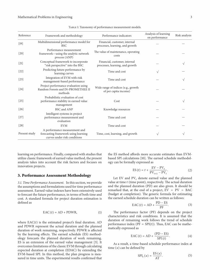
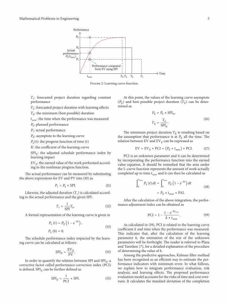
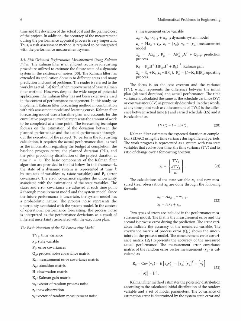
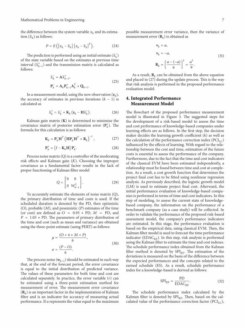
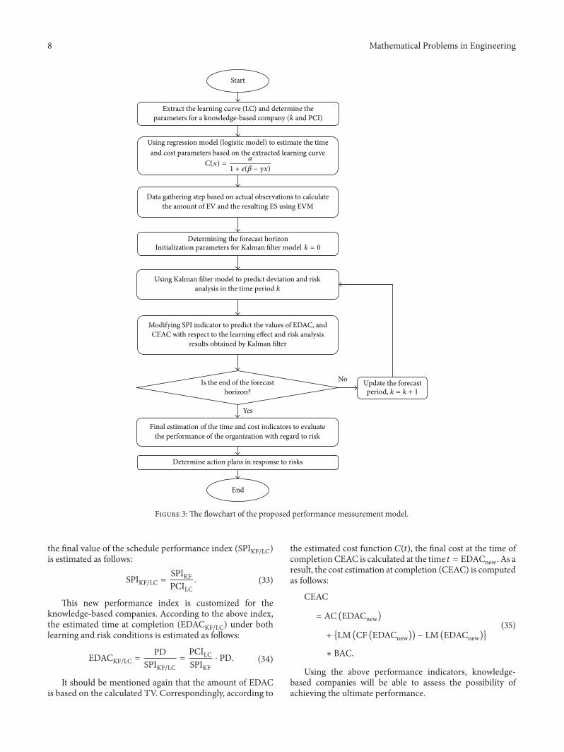
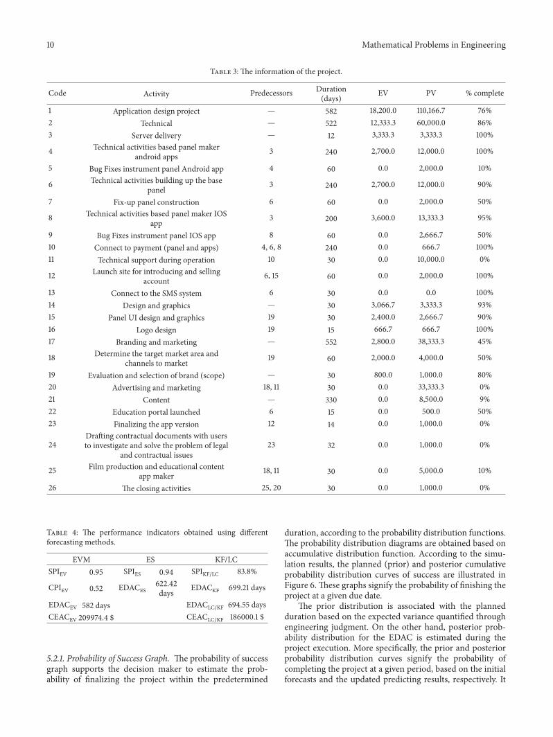
Related Documents


