IT 13 019 Examensarbete 30 hp Mars 2013 Research and optimization of a H.264AVC motion estimation algorithm based on a 3G network Ou Yu Institutionen för informationsteknologi Department of Information Technology

Welcome message from author
This document is posted to help you gain knowledge. Please leave a comment to let me know what you think about it! Share it to your friends and learn new things together.
Transcript
IT 13 019
Examensarbete 30 hpMars 2013
Research and optimization of a H.264AVC motion estimation algorithm based on a 3G network
Ou Yu
Institutionen för informationsteknologiDepartment of Information Technology

Teknisk- naturvetenskaplig fakultet UTH-enheten Besöksadress: Ångströmlaboratoriet Lägerhyddsvägen 1 Hus 4, Plan 0 Postadress: Box 536 751 21 Uppsala Telefon: 018 – 471 30 03 Telefax: 018 – 471 30 00 Hemsida: http://www.teknat.uu.se/student
Abstract
Research and optimization of a H.264AVC motionestimation algorithm based on a 3G network
Ou Yu
The new video codec standard H.264/AVC is jointly developed by ISO/IEC MovingPicture Expert Group MPEG and ITU-T Video Coding Experts Group [1] [2], VCEG.It has higher coding efficiency than the MPEG-4, thus could be applied to highdefinition application in low bit-rate wireless environment.[3] However H.264/AVChas harsh requirement on the hardware, basically due to the complexity of thealgorithms it used. And end devices, e.g. smart phones usually do not have sufficientcomputing capability, also it is restricted by limited battery power. As a result, it iscrucial to reduce the computing complexity of H.264/AVC codec, and in the sametime, keep the video quality unharmed.
After the analysis of the H.264/AVC coding algorithm, it can be found that ME(motion estimation) consumes the biggest part of the computing power. So in orderto adopt H.264/AVC to real-time, low bit-rate video application, it is very importantto optimize ME algorithm. In this thesis, basic knowledge and key technology ofH.264/AVC is introduced in the first place. Then it systematically illustrate theexisting block-matching ME algorithms, both the algorithm flow and differenttechnology involved, also the pros and cons of each. In the next part, a very famousalgorithm UMHexagonS, now accepted by ITU-T, is introduced in detail, and theauthor explain in different aspects why this algorithm could gain more efficiency overothers. And on the base of the analysis, the author proposes some improvement tothe UMHexagonS, taking thoughts of some classic ME algorithms into it. In the lastphase of the thesis, both Subjective quality assessment experiment and objectivequality assessment experiment are used to examine the performance of the improvedalgorithm. It has been shown by experiments that the improved ME algorithmrequires less computing power than UMHexagonS, while keeping video quality at thesame level. The improved algorithm could be used in a wireless environment such as a3G network.
Tryckt av: Reprocentralen ITCIT 13 019Examinator: Ivan ChristoffÄmnesgranskare: Ivan ChristoffHandledare: Huijuan Zhang

Table of Contents
1 Introduction ...................................................................................................................... 1
1.1 Background ............................................................................................................ 1
1.2 Related Works ........................................................................................................ 2
1.3 Thesis Outline ......................................................................................................... 4
2 Principle of Block-Based Motion Estimation Algorithm ................................................. 5
2.1 Introduction of the H.264/AVC Standard ............................................................... 5
2.2 Encoder and Decoder of the H.264/AVC Standard................................................ 6
2.3 Motion Estimation Theory ..................................................................................... 7
2.3.1 Basic concept on Motion Estimation ........................................................... 8
2.3.2 Key Principle of Motion Estimation ........................................................... 11
2.3.3 The Matching Criterion .............................................................................. 12
2.4 Summary .............................................................................................................. 13
3 Analysis of the Classic Motion Estimation Algorithm .................................................... 15
3.1 Full Search............................................................................................................ 15
3.2 Three Step Search ................................................................................................. 16
3.3 Four Step Search .................................................................................................. 17
3.4 Block Based Gradient Descent Search ................................................................. 18
3.5 Diamond Search ................................................................................................... 18
3.6 Motion Vector Field Adaptive Search ................................................................... 19
3.7 Summary .............................................................................................................. 21
4 Analysis and Optimization of Unsymmetrical Multi Hexagon Search ........................... 23
4.1 Analysis of Unsymmetrical Multi Hexagon Search ............................................. 23
4.2 Optimization of Unsymmetrical Multi Hexagon Search ..................................... 27
4.3 Optimization Details of Unsymmetrical Multi Hexagon Search ......................... 28
4.3.1 Optimization on Early Termination ............................................................ 28
4.3.2 Adoption of Movement Intensity ................................................................ 30
4.4 Implementation of the Algorithm ......................................................................... 32
4.4.1 Starting Point Prediction ............................................................................. 32
4.4.2 Search Pattern ............................................................................................. 33
4.4.3 Search Process ............................................................................................ 34
4.5 Summary .............................................................................................................. 34
5 Experiment Proof of Improved Algorithm ..................................................................... 37
5.1 Objective Quality Assessment based on JM Model ............................................. 37
5.1.1 Design of the Experiment ........................................................................... 37
5.1.2 Analysis of the Result ................................................................................. 38
5.2 Subjective Quality Assessment Using Double Stimulus Impairment Scale ........ 40
5.2.1 Design of Experiment ................................................................................. 40
5.2.2 Analysis of the Result ................................................................................. 41
5.3 Summary .............................................................................................................. 42
6 Conclusion ...................................................................................................................... 43
References ......................................................................................................................... 44
1
Chapter1 Introduction
1.1 Background
As more and more Telecommunication Service Providers (TSP) start to promote their
3G network business, the coverage of 3G network is rocketing up in China.[4] And it
is expected that two years from now, 9 cellphones out of 10 will use 3G network. By
the mean time streaming video, one of the most distinguishing features of 3G network,
will be the battle field for Telecommunication Service Providers to gain their
maximum benefits.
Traditional online streaming media usually uses early coding method. The size of the
media file is quite small, and correspondingly, the image quality is quite vague. Now,
the new generation of high-definition coding standard, H.264/AVC video coding
standard can provide better video quality in the same bit rate. And network abstraction
layer is added in the coding standard, to make it more convenient for the production
of Internet streaming application. Therefore, the technology is quite suitable for 3G
mobile multimedia usage.
However, to apply H.264/AVC coding standard efficiently on 3G platform, there are
mainly four obstacles need to be conquered, including power-consumption control,
error control, transmission rate control, compression efficiency.
The main power control problem to be solved is how to reduce the power that
streaming media tasks require, so as to extend battery life. In a mobile wireless video
transmission system, the mobile terminal not only needs to do decoding to receive
video, and also needs to encode to send video. So power control problem can be
divided into two aspects. [5]
Fault-tolerant technology is an essential part in wireless video transmission. Due to
the QoS (Quality of Service) of 3G wireless channel, fault-tolerant technology is very
crucial to ensure the accuracy and completeness of data transmission. It usually
includes lost data recovery and concealment.
Video encoding is also crucial for video communication, because the wireless channel
bandwidth is limited. And there should be balance between video content size and
output quality, and also ensure good and stable quality on the receiving end,
Compression efficiency is an important video encoding parameter. Better
2
compression efficiency means better video quality under same video file size. But at
the same time, better compression efficiency is gained at the cost of higher
complexity of coding algorithm, which leads to more computing power consumption.
For now, the CPU, memory and other hardware of an ordinary 3G phone cannot
compete with mainstream personal computer. So if we do not adjust video coding
algorithm, it will certainly not meet the mobile video platforms in 3G mobile use, not
to mention real-time encoding applications, such as video calls.
This thesis put its focus on the compression efficiency, trying to find a balanced way
to simplify the complexity of the algorithm, and in the same time not harm the video
quality significantly.
1.2 Related Works
The data compression of video signals is carried out by reducing the redundant signals.
Video signals contain two types of redundancy: statistical redundancy (also known as
spatial redundancy) and human visual redundancy. Spatial redundancy, or geometric
redundancy, is caused by the correlation between adjacent pixels. This kind of
redundancy can be erased by changing the mapping rule of the relevant pixels. For
example, if the background of the video has only one color, there will be a lot of
spatial redundancy. The other kind of redundancy, psychological redundancy, which
is caused by the nature of human visual system. Because human visual system is not
sensitive to a number of frequency component in the video. For example, human
cannot notice slightly color changes in the video. For both kinds of redundancy, the
greater the amount of redundancy is, the higher possibility of compressibility will be.
In current situation, the bandwidth of 3G network is still a bottle-neck for high quality
video transmission. Therefore, how to improve the compression efficiency of video
coding is very crucial. And many research papers are focusing on how to reduce the
complexity of coding, while ensuring the quality of coding. And most of the papers
mentioned fast motion estimation algorithm. During video compression period, more
than half of the time is spent on motion estimation (ME). The basic idea of motion
estimation is firstly to divide each frame into non-overlapping macroblocks. And then
each macroblock can find its reference macroblock in certain frames. By doing this, a
large amount of residual can be removed.
Block-matching motion estimation has its advantage over other ME algorithms,
3
including recursive estimation, Bayesian estimation and optical flow method. Because
the concept of this algorithm is more straight forward, and it is easy to implement. So
now many researchers put their energy on block-matching motion estimation, trying
to make a breakthrough in video compression efficiency. There are several classic
block-based motion estimation algorithms. Theoretically, full search algorithm (FS)
[6] is the most accurate block-matching algorithm, because it searches all the block
pixel-by-pixel to get the best motion vector (MV). But limited by the high
computational complexity, the full search is not the ideal method for real-time usage.
Later, some fast search algorithms are made to meet real-time requirement.
Three-Step Search (TSS) [7]reduces the amount of computation by reducing the
number of search pixel, but its relatively large initial search step impairs the
performance. Some many other algorithms, New Three-Step Search (NTSS)[8], New
Four-Step Search (NFSS)[9], Block-Based Gradient Descent Search (BBGDS) [10]
[11]take use of the motion vector distribution offset, greatly improved the speed and
efficiency in low-complexity video usage.
October 1999, Diamond (DS) [12]search algorithm is adopted by MPEG-4
verification model. Although the diamond method has superior overall performance
than other algorithms, and the application of DS was a big success. But still, the
performance in some particular case, for example, this algorithm does not provide
flexible way to deal with different video content, and it is easy to fall into local
optimization, which in return impacts the search performance and coding efficiency.
Hexagon Search (HEXBS) [13] is another advanced algorithm. It uses relatively large
search box and fast-moving module to reduce the search times, much less than
Diamond Search. But HEXBS also did not consider the motion vector correlation,
thus cannot handle video with intense movement quite well. Adaptive Motion Vector
Search (MVFAST) and Predicted Motion Vector Adaptive Search (PMVFAST) [14]
are included in 2001, MPEG-4 video standard. Both of algorithms use motion
correlation and related content based on movement and features to choose different
search modes, in addition, it use prediction vector and other new concept such as,
early termination, to improve both search speed and video quality. But still like
other algorithms mentioned above, these two algorithms cannot handle video with
intense movement quite well.
In chapter 3, all the algorithms mentioned above will be analyzed in detail. And based
on this, a new, hybrid algorithm will be introduced which is more suitable for 3G
4
mobile platform.
1.3 Thesis Outline
Chapter 1 is the introduction part. It covers the difficult point to apply video coding
technology to 3G network usage. Then it summarizes the current study focus, and
from which leads out to the study focus of this thesis.
Chapter 2 focuses on the basic principle and framework of H.264/AVC, especially the
motion estimation.
Chapter 3 introduces several classic motion estimation algorithms, and then analyzes
the pros and cons of each individual algorithm.
In Chapter 4, a motion estimation algorithm called UMHexagonS is analyzed. And
based on it, this thesis brings some improvements to it. And this chapter explains the
whole improvement process in detail.
Chapter 5 is the experiment proof. This thesis uses both objective and subjective ways
to prove that the improved algorithms can reduce the complexity of the motion
estimation while in the same time keep the video quality unharmed.
Chapter 6 is the conclusion.
5
Chapter2 Principle of Block-Based Motion Estimation
Algorithm
2.1 Introduction of the H.264/AVC Standard
MPEG (Moving Picture Experts Group) and VCEG (Video Coding Experts Group) have
jointly developed AVC (Advanced Video Coding), which is better than any early
video codec, like MPEG and H.263. This video codec is also known as ITU-T Rec. H.264
and MPEG-4 Part 10 standard. Here, in short, we name it H.264 /AVC or H.264. This
international standard was ITU-T adopted and officially promulgated on March, 2003. It is
widely believed that the promulgation of H.264 is a major event in the development of
video compression coding discipline and its superior compression performance will also
play an important role in all aspects of digital television broadcasting, video, real-time
communication, network video streaming delivery and multimedia messaging. Specifically,
compared with other video coding technology H.264 AVC has the following advantages:
1. Higher coding efficiency: compared with the H.263, it can save approximately
50% of the bit rate while providing the same video quality.
2. The quality of the video: H.264 can provide high-quality video images on low bit rate
channel, like 3G network, for example.
3. Improvement of network adaptability: H.264 can work in real-time, low-latency
communications applications. (Such as video conferencing) And can also be used for no
delay video storage or video streaming server.
4. Using of hybrid coding structure: similar with H.263, H.264 also use DCT
transform coding plus the DPCM coding structure. And it uses several advanced
technology, such as multi-mode motion estimation, intra prediction, multi-frame prediction,
variable length coding based on the contents, 4x4 two-dimensional integer transform new
coding method to improve the coding efficiency.
5. Less encoding options: it often needs to set quite a lot of options in H.263, which
increases the difficulty of encoding. H.264 tries to be brief "back to basics" and
reduce the encoding complexity.
6. Adaptable for different occasions: H.264 can use different transmission and playback
rate depending on the environment, and also provides a wealth of error-handling
tools, you can control or eliminate packet loss and bit error.
6
7. Error recovery: H.264 provides the tools to solve the problem of network
transmission packet loss, especially in a wireless network, which has high bit error
rate.
8. Higher degree of complexity: H.264 improves its performance by increasing the
complexity. It is estimated that the computational complexity of H.264 encoding is
roughly equivalent to three times that of the H.263. And decoding complexity is
roughly equivalent to two times that of the H.263.
2.2 Encoder and Decoder of the H.264/AVC Standard
H.264/AVC does not give a specific implementation instruction of the encoder and
decoder, but only provide a set of semantics and rules. And different encoders and
decoders from different providers can work under the predefined framework. This can
encourage the positive competition among providers.
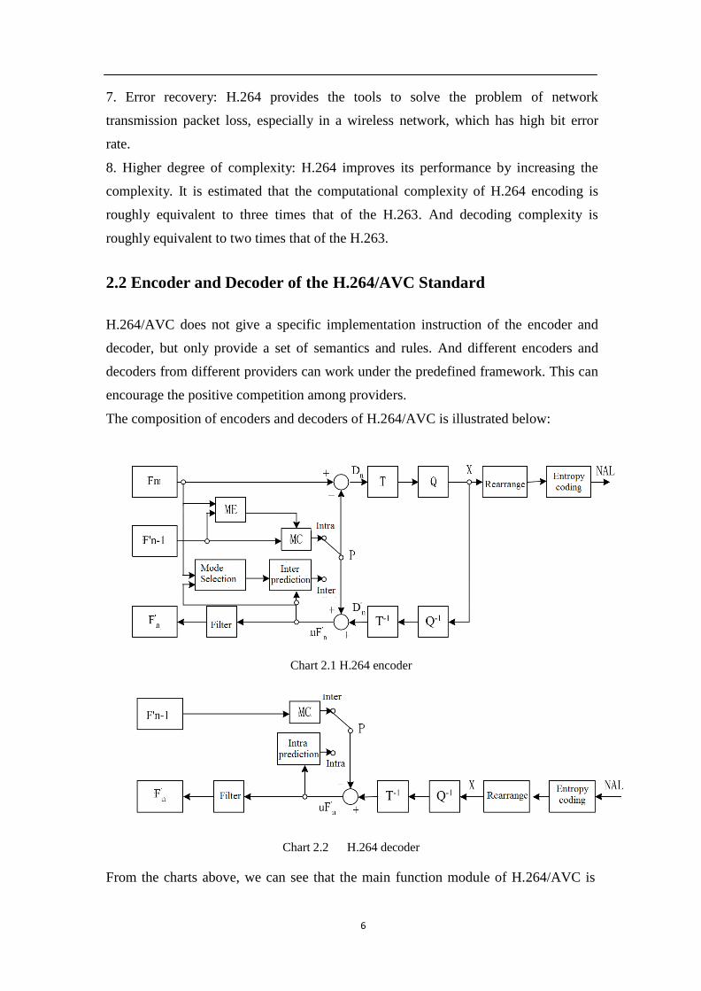
The composition of encoders and decoders of H.264/AVC is illustrated below:
Chart 2.1 H.264 encoder
Chart 2.2 H.264 decoder
From the charts above, we can see that the main function module of H.264/AVC is
7
'
'
n D
similar to former standards, e.g. H.261, H.263, MPEG-1 and MPEG-4. The main
difference lies in the detail of each function module.
Encoder uses a hybrid coding method of transform and prediction. The input filed, or
frame Fn is processed in unit of macroblock. And there are two ways of predictions
in this stage. They are inter-frame prediction and intra-frame prediction. If intra-frame
prediction is adopted, the predicted value PRED (represented as P) is calculated from
the previous macroblock within current frame through motion compensation (MC).
And the reference block is marked as Fn 1 . Another way is inter-frame prediction,
which is more precise and compression efficient. The reference block can be either
the past frame or the frame in the future. Subtract the PRED from the current block,
we can gain a residual block ( Dn ). Then through transform and quantization,
transform coefficients X is calculated. And after entropy coding and adding some side
information like motion vector and quantization parameter, the final stream can be
transferred through NAL for transition or storage purpose. And in order to provide the
reference image for further prediction, the encoder also need to have the ability to
rebuild image. So the residual image can be inverse quantized and inverse
transformed to Dn . And we can get the unfiltered frame
uF '
'
by adding n
'
with P.
And after some noise removing, we can get the rebuilt frame Fn .
And Chart 2.2 is the reversed process of Chart 2.1, the input is the H.264/AVC stream, '
and after the reversed process, the current frame
the final image signal.
2.3 Motion Estimation Theory
Fn can be extracted and then output
Motion estimation is the process to predict the movement trend of the image from
inter-frames. Thus, it can use a smaller amount of information (image change) to
describe the entire image. Currently, motion estimation algorithm is divided into three
categories:
l. Pixel-based motion estimation
This type of motion estimation algorithm uses pixels as the basic unit, to describe the
different state of motion of each pixel. [15]This algorithm is highly precise, but also
with high computational complexity that it is difficult to achieve real-time encoding.
So it cannot be used in real-time scenario.
2. Object-based motion estimation
8
Object-based motion estimation usually split video images, to create a number of
objects, and then to track and match these objects. This algorithm highly depends on
video object segmentation algorithm, which is not considered to be mature enough.
As a result, the progress in object-based motion estimation research is quite slow. And
also, split object may be of different sizes, without any rules in common, leading to
the higher complexity of the algorithm. And such kind of design cannot achieve
practical purposes.
3. Block-based motion estimation
Block-based motion estimation uses blocks as the basic unit, each block contains a
number of pixels, and assuming that all pixels within each block has a consistent state
of motion. Because it uses block as a unit, the computational complexity of motion
estimation can be greatly reduced.
In addition, there are also studies about how to improve the encoding quality of the
work according to the characteristics of the human eye, for example, there is a coding
method that skips the non-sensible video content to allocate more bits on sensible
content to obtain better overall video quality.
This thesis will focus on the block-based motion estimation, and in the next section,
basic principle of block matching motion estimation will be introduced.
2.3.1 Basic concept on Motion Estimation
Like any other video coding technology, H.264/AVC is built upon several basic
concepts. First, let me introduce those important concepts.
Field and Frame
Field or frame of the video can be used to generate an encoded image. Typically, a
video frame may be divided into two types: continuous or interlaced video frame. In
traditional television, a frame is divided into two interlaced field, in order to reduce
the blinking of the video image. Usually, video content with low motion movement
should adopt frame coding mode, while those with fierce movements should uses
field coding mode.
Macroblock
A coded image can be divided into several macroblocks, and each macroblock
9
consists of a 16 x 16 array of luminance (Y) pixels and some Chroma pixels (Cr, Cb) ,
which depend on the indicator in the sequence header. And several macroblocks can
form a slice. In Slice I, there is only Macroblock I. Slice P can contain Macroblock P
and Macroblock I. And Slice B can contain Macroblock B and Macroblock I.
Macroblock I can only uses coded pixels in current slice to perform intra-frame
prediction.
Macroblock P can uses previously coded image to do inter-frame prediction. The
macroblock can be divided into 16×16, 16×8,8×16, or 8×8. And it can be further
divided into small blocks, for example, if 8×8 mode is chosen, you can choose the
sub-block size like 8×8, 8×4, 4×8 or 4×4.
Macroblock B is similar to P, but it can also use the future image to do inter-frame
prediction.
Motion Vector
In inter-frame prediction, every MB is predicted from a certain same sized MB in
reference frame. And the vector among these two is called Motion Vector (MV). It
has 1/4 pixel accuracy with Luminance component and 1/8 pixel precision with
chroma component. As a result, the reference pixel might not really exist in reference
frame (if the MV is not integer), but using interpolation operation to gain the result.
The transmission of each MV requires certain amount of bits, especially for
small-sized block size. In order to reduce the bits rate, we can use adjacent MV to
predict current MV, because adjacent MV has high correlation. And there only needs
to transmit the differential of the MV (MVD), instead of transmit the whole MV
(MVP). By doing this, we can save large amount of bit rate.
Chart 2.3 Current MB and adjacent MBs (in same size)
10
As shown above, E is the current macroblock or sub-macroblock. A B C is the
adjacent macroblock on the left, top and top right. If there is more than one macro
block on the left (chart 2.4), A, which is on the top is used as reference. And B, which
is the left of the top adjacent macroblocks, is chosen to be the reference block.
Chart 2.4 Current MB and adjacent MBs (in different sizes)
In Chart 2.4, if
The block size is not 16×8 or 8×16, the MVP is the average of MV from A, B and C.
If the block size is 16×8, the MVP of the upper part is from B, and the bottom is
from A.
If the block size is 8×16, the MVP of the left part is from A, and the right is from
C.
Motion Compensation
Motion compensation describes the process of turning reference picture to current
picture. The segmentation of Macroblocks (mentioned above) increases the
correlation of each macroblocks or sub-macroblocks, thus providing the possibility
for more efficient motion compensation, which is called tree structured motion
compensation. For each macroblocks or sub-macroblocks, it has to have motion
compensation for individual. And every MV has to be encoded, transferred, and
integrated into the output stream. For large sized MB, the MV and segmentation type
only takes small proportion of the whole stream, while the motion compensation takes
the biggest part, because the details of a large sized MB is more complex than small
sized one. And on the contrast, the MV and segmentation type takes the biggest part
for those small sized MB. So small sized MB is suitable for the image with more
details, and large sized MB is suitable for those with little or no details.
As is show in Chart 2.5, the H.264/AVC encoder chooses the segmentation type for
each block on a residual frame, which has not been through motion compensation yet.
And for the grey background image, it uses big sized block like 16×16. But in the
11
detailed part, for example, face and hair, it uses small sized block to gain a better
encoding efficiency.
2.3.2 Key Principle of Motion Estimation
In normal cases, adjacent frames within a video content is correlated, thus exists
redundancy, as illustrated by Shannon information theory. As a matter of fact, there is
redundancy for almost every video content. And it provides possibility for video
compression and video encoding technology.
Chart 2.5 Residual frame
Using inter-frame prediction technology can erase the redundancy created by frame
correlation. The same pixel in the previous frame has reference value for current
frames for still image. And for the image that is on the move, we should take motion
vector into consideration. So we need to find the matched pixel or MB in previous or
future frame, which have reference value for current frame. And the process of
finding the matched pixel or MB is called motion estimation. Motion estimation can
erase the redundancy by large amount, thus lower the information to encode and also
lower the time estimation for encoding.
As is shown in Chart 2.6, the practice of motion estimation is first to divide image
into individual MBs. Assuming all the pixel within MB has the same MV, then it
searches for the matched MB on the previous or future frames based on pre-defined
matching criterion. And the vector between current MB and matched MB is called
motion vector. And next step is to calculate the differential between motion
compensation and compensation residuals, which will be further transformed,
12
quantized, encoded and transferred.
Chart 2.6 Illustration of motion estimation
2.3.3 The Matching Criterion
There are four types of matching criterion for block matching [16]:
Minimum Mean Square Error (MSE), Minimum Absolute Difference MAD,
Normalized Cross-Correlation Function (NCCF), and Absolute Error (SAD)
Minimum Mean Square Error (MSE)
(2-1)
(i,j) refers to the motion vector, f k
and f k 1
is the grey value of each pixel in
current and previous frame. MN is the size of the block. The MB with lowest MSE is
selected to be the matched MB.
Minimum absolute difference (MAD)
(2-2)
MB with lowest MAD is the matched MB.
Normalized Cross-Correlation Function (NCCF)
(2-3)
B with highest NCCF is the matched MB.
2
1
1
1
]),(),([1
).(
M
m
k
N
n
k jnimfnmfMN
jiMSE
|),(),(|1
).(1
1
1
M
m
k
N
n
k jnimfnmfMN
jiMAD
21
21
1 1
12
11
2
1
1
1
]),([)],([
),(),(
).(
M
m
M
m
k
N
n
N
n
k
M
m
k
N
n
k
jnimfnmf
jnimfnmf
jiNCCF
13
Absolute Error (SAD)
(2-4)
And MB with lowest SAD is selected to be the matched MB. In practice, matching
criterion does not play a vital role to the precision of the matching process.
And because SAD is easier to implement, and it requires low computing power. SAD
is often chosen for the matching criterion.
2.4 Summary
This chapter is the introduction part. It introduces the basic concept of H.264/AVC
video encoding technology. And some of the key technologies like motion
compensation and motion estimation are introduced in detail.
|),(),(|).(1
1
1
M
m
k
N
n
k jnimfnmfjiSAD

14
15
Chapter 3 Analysis of the Classic Motion Estimation
Algorithm
Since the birth of video codec technology, motion estimation algorithm has become
one of the most important elements. The efficiency of the motion estimation
algorithm largely affects the success or failure of the video encoding technology. In
the development of the block-matching motion algorithm, there comes many
innovative, highly efficient algorithms, and many of those have been replaced by
more efficient algorithm. But the thought of those algorithms has become classic. This
chapter will analyze some classic motion estimation algorithm.
3.1 Full Search
`
Chart 3.1 Full search process
Chart 3.1 illustrates the process to find the best motion vector in Full Search
algorithm. The algorithm start the search from the origin of the image (generally
upper left), in a pre-made search box, all possible search block and compared with the
current block. And then to choose the most appropriate prediction block. The offset of
the two blocks is the motion estimation vector MV (u, v). Full search algorithm search
for all possible blocks, so the search accuracy is the best. But the search volume is too
large, it is difficult to meet the needs for real-time encoding.
16
3.2 Three Step Search
The process of the three-step search algorithm is shown in Figure 3.2, the center point
of the a 16x16 search box, (i, j) is set to the origin (0,0). The initial search step size is
set to the half of the maximum step. Then the MAD values of (i, j) points and their
peripheral eight neighboring points are calculated. And the point with smallest MAD
is set to be the new search center point. Then the second search step is changed to half
of the original search step and then repeats the process again, until the point with
smallest MAD is found. And the offset is set to be the motion vector.
The three-step search algorithm is highly efficient, but because its search process
design is too simple, it cannot be guaranteed that optimal motion vector can be found.
Chart 3.2 Three step search process
17
3.3 Four Step Search
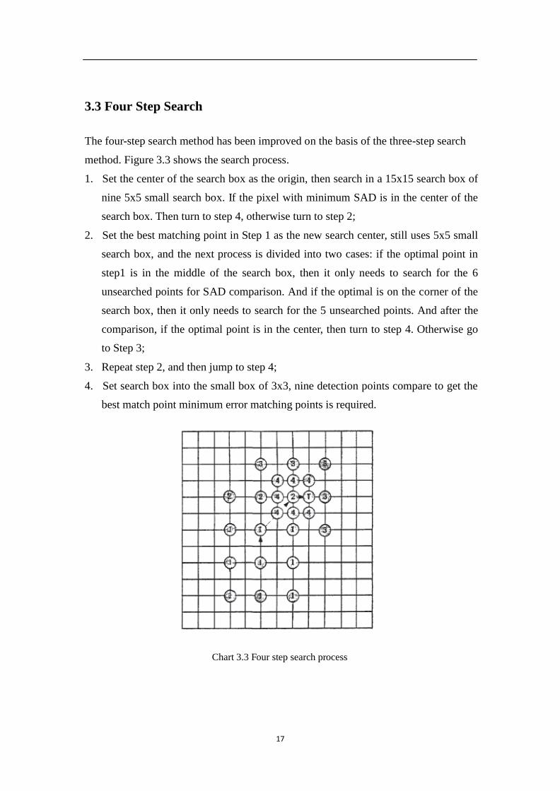
The four-step search method has been improved on the basis of the three-step search
method. Figure 3.3 shows the search process.
1. Set the center of the search box as the origin, then search in a 15x15 search box of
nine 5x5 small search box. If the pixel with minimum SAD is in the center of the
search box. Then turn to step 4, otherwise turn to step 2;
2. Set the best matching point in Step 1 as the new search center, still uses 5x5 small
search box, and the next process is divided into two cases: if the optimal point in
step1 is in the middle of the search box, then it only needs to search for the 6
unsearched points for SAD comparison. And if the optimal is on the corner of the
search box, then it only needs to search for the 5 unsearched points. And after the
comparison, if the optimal point is in the center, then turn to step 4. Otherwise go
to Step 3;
3. Repeat step 2, and then jump to step 4;
4. Set search box into the small box of 3x3, nine detection points compare to get the
best match point minimum error matching points is required.
Chart 3.3 Four step search process
18
3.4 Block Based Gradient Descent Search
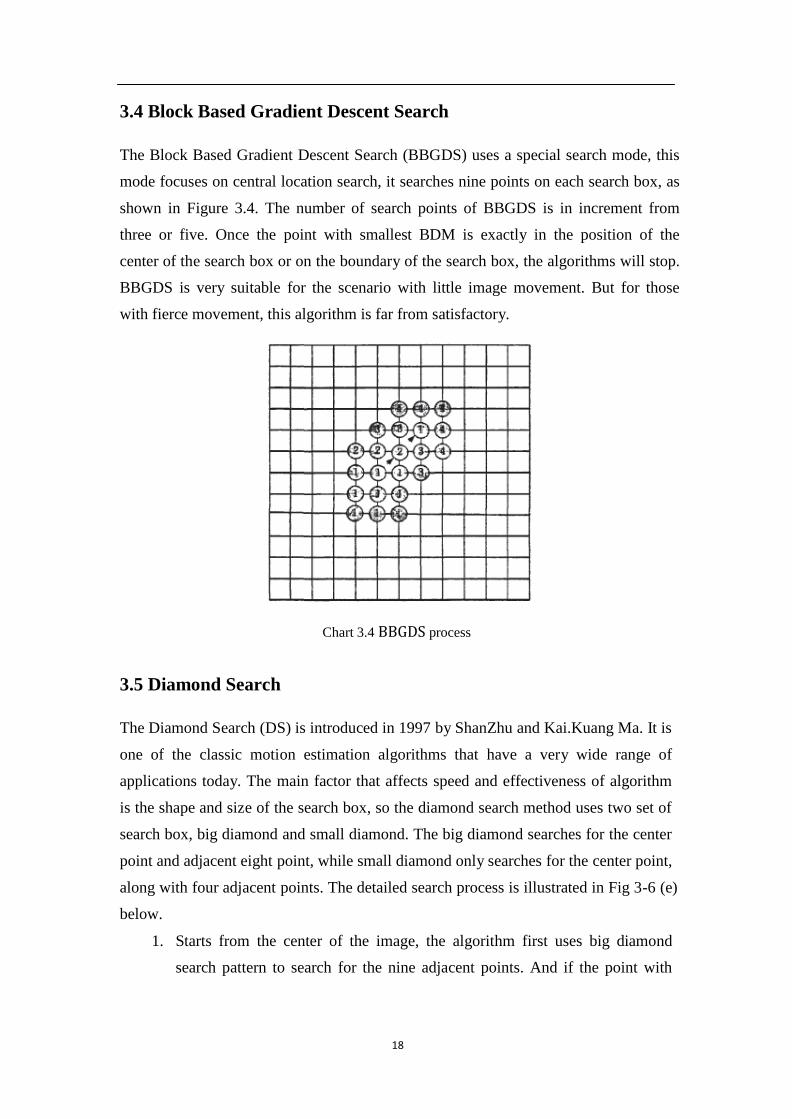
The Block Based Gradient Descent Search (BBGDS) uses a special search mode, this
mode focuses on central location search, it searches nine points on each search box, as
shown in Figure 3.4. The number of search points of BBGDS is in increment from
three or five. Once the point with smallest BDM is exactly in the position of the
center of the search box or on the boundary of the search box, the algorithms will stop.
BBGDS is very suitable for the scenario with little image movement. But for those
with fierce movement, this algorithm is far from satisfactory.
Chart 3.4 BBGDS process
3.5 Diamond Search
The Diamond Search (DS) is introduced in 1997 by ShanZhu and Kai.Kuang Ma. It is
one of the classic motion estimation algorithms that have a very wide range of
applications today. The main factor that affects speed and effectiveness of algorithm
is the shape and size of the search box, so the diamond search method uses two set of
search box, big diamond and small diamond. The big diamond searches for the center
point and adjacent eight point, while small diamond only searches for the center point,
along with four adjacent points. The detailed search process is illustrated in Fig 3-6 (e)
below.
1. Starts from the center of the image, the algorithm first uses big diamond
search pattern to search for the nine adjacent points. And if the point with
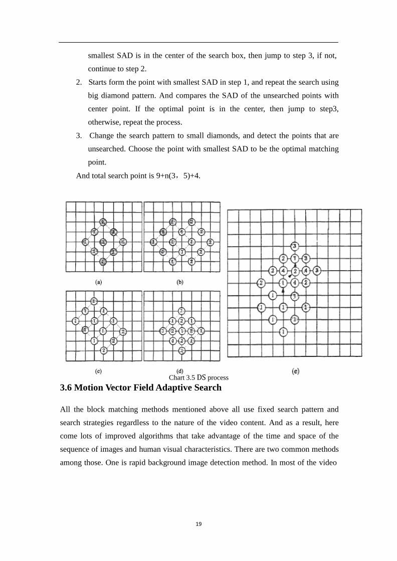
19
smallest SAD is in the center of the search box, then jump to step 3, if not,
continue to step 2.
2. Starts form the point with smallest SAD in step 1, and repeat the search using
big diamond pattern. And compares the SAD of the unsearched points with
center point. If the optimal point is in the center, then jump to step3,
otherwise, repeat the process.
3. Change the search pattern to small diamonds, and detect the points that are
unsearched. Choose the point with smallest SAD to be the optimal matching
point.
And total search point is 9+n(3,5)+4.
Chart 3.5 DS process
3.6 Motion Vector Field Adaptive Search
All the block matching methods mentioned above all use fixed search pattern and
search strategies regardless to the nature of the video content. And as a result, here
come lots of improved algorithms that take advantage of the time and space of the
sequence of images and human visual characteristics. There are two common methods
among those. One is rapid background image detection method. In most of the video
20
sequence, the background of the image takes biggest property of the whole, and if we
can quickly detect the background, then we can reduce the computing time by big
margin. For example, we can directly calculate the SAD value of the zero vector
(Starting point), and if the SAD value is less than a certain threshold value T, then
directly terminate the search, and the zero vector is the final motion vector. In such a
way, we can only perform single time of search to locate the optimal point, and by
doing this we can improve the efficiency of the algorithms.
Another common method is based on prediction of the complexity of current block
movement. Different search patterns will be applied to different complexity of block
movement. If the motion vector of the adjacent blocks are comparably high, then the
current block are considered to be in fierce movement. In this case, big search box
pattern are applied, such as DS and hexagon search, otherwise only use small search
pattern to complete the search. And this is the basic idea of the motion vector field
adaptive search algorithm (MVFAST), which is quite a breakthrough in fast motion
estimation algorithms.
1. Still MB detection
Most of the still MB in any video sequence has the MV of (0,0). And those still MB
can be detected using SAD. If SAD of pixel (0,0) is smaller than a threshold T, then
this MB can be considered to be still, and the search can come to an end, which is
called early termination. And (0, 0) is the motion vector. And in MVFAST, this
threshold is set to 512, and it is configurable. If it is set to 0, then the early termination
process will be skipped.
2. Movement intensity
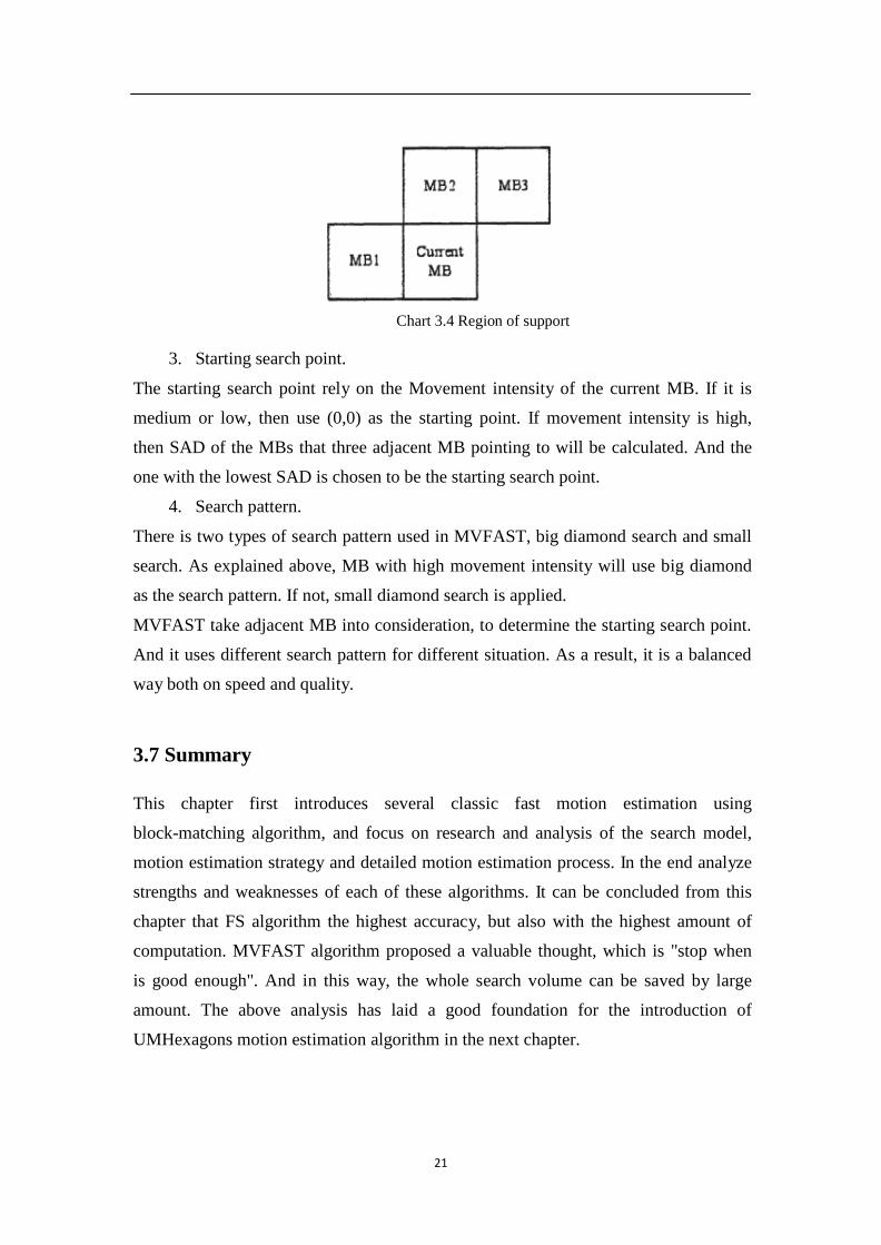
In MVFAST, the movement intensity of a MB can be defined by the MV of Region
of Support (ROS). ROS is the adjacent MB on the left, top and top right. Assuming
Vi=(xi , yi) is the MV of MBl,MB2,MB3. And Li | xi | | yi |, L max( Li ) . Then
the movement intensity of current MB can be defined below.
Movement intensity=low, L L1
= medium, L1 L L2
=high, L L2 ( L1 , L2 can be pre-defined) (3.1)
21
Chart 3.4 Region of support
3. Starting search point.
The starting search point rely on the Movement intensity of the current MB. If it is
medium or low, then use (0,0) as the starting point. If movement intensity is high,
then SAD of the MBs that three adjacent MB pointing to will be calculated. And the
one with the lowest SAD is chosen to be the starting search point.
4. Search pattern.
There is two types of search pattern used in MVFAST, big diamond search and small
search. As explained above, MB with high movement intensity will use big diamond
as the search pattern. If not, small diamond search is applied.
MVFAST take adjacent MB into consideration, to determine the starting search point.
And it uses different search pattern for different situation. As a result, it is a balanced
way both on speed and quality.
3.7 Summary
This chapter first introduces several classic fast motion estimation using
block-matching algorithm, and focus on research and analysis of the search model,
motion estimation strategy and detailed motion estimation process. In the end analyze
strengths and weaknesses of each of these algorithms. It can be concluded from this
chapter that FS algorithm the highest accuracy, but also with the highest amount of
computation. MVFAST algorithm proposed a valuable thought, which is "stop when
is good enough". And in this way, the whole search volume can be saved by large
amount. The above analysis has laid a good foundation for the introduction of
UMHexagons motion estimation algorithm in the next chapter.

22

23
Chapter 4 Analysis and Optimization of Unsymmetrical Multi
Hexagon Search
4.1 Analysis of Unsymmetrical Multi Hexagon Search
Some of the motion estimation algorithms mentioned above, such as TSS, FSS, DS,
HS, all aims to reduce the search volume by means of limit the search points. And
those algorithms can gain good efficiency if the size of the video content is small.
But while dealing with some of the large-size images and a larger search range, those
fast search algorithms tend to fall into local optimization, and thereby seriously
affecting the coding efficiency. Therefore, this chapter focuses on the Unsymmetrical
Multi Hexagon Search (UMHexagonS) [17] algorithm. This algorithm can save up
to
90% of the computing complexity compared to Full Search. And it uses multi-level,
different shapes of search pattern, which can prevent from falling in local
optimization.
UMHexagonS algorithm also uses SAD as its matching criterion. And it uses early
termination mechanism. In most cases, the best matching point is very close to the
initial prediction point, which means that in many cases, the motion estimation search
is superfluous. And in this early termination mechanism, the threshold value is mainly
affected by two factors: the current adjustment factor (β), ------and the predicted
motion compensation ( m cos t pred ). The threshold values are defined as follows
Threshold A m cos t pred (1 1 )
Threshold B m cos t pred (1 2 )
(4.1)
(4.2)
If ThresholdB
is met, then the algorithm skips Step 3, and directly jump to Step4_2.
And if it only meet the requirement for Threshold A , it needs to perform Step4_1
before Step4_2. And the whole process is illustrated in Chart 4.1.
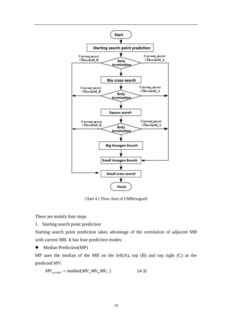
24
Chart 4.1 Flow chart of UMHexagonS
There are mainly four steps
1. Starting search point prediction
Starting search point prediction takes advantage of the correlation of adjacent MB
with current MB. It has four prediction modes:
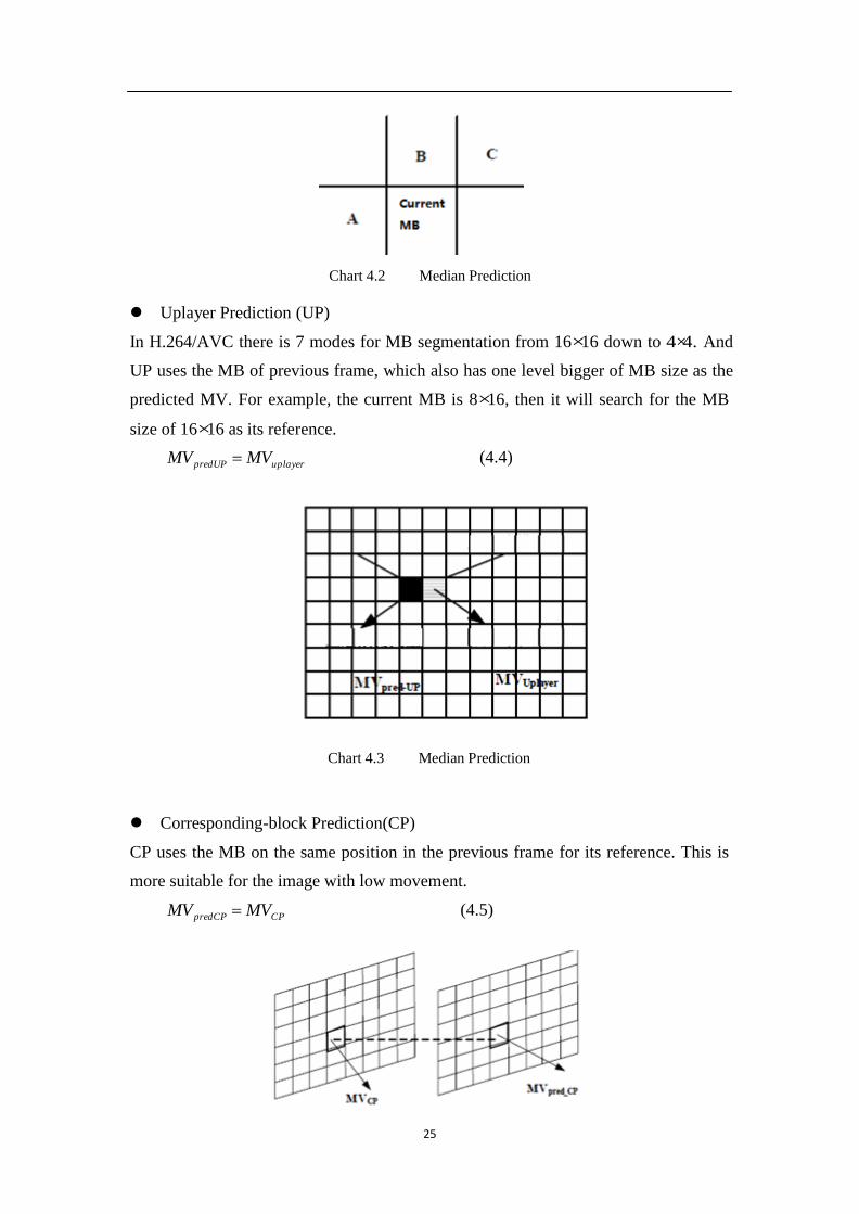
Median Prediction(MP)
MP uses the median of the MB on the left(A), top (B) and top right (C) as the
predicted MV.
MVpredMP median[MVA MVB MVC ]
(4.3)
25
Chart 4.4 Corresponding-block Prediction
Chart 4.2 Median Prediction
Uplayer Prediction (UP)
In H.264/AVC there is 7 modes for MB segmentation from 16×16 down to 4×4. And
UP uses the MB of previous frame, which also has one level bigger of MB size as the
predicted MV. For example, the current MB is 8×16, then it will search for the MB
size of 16×16 as its reference.
MV predUP MVuplayer
(4.4)
Chart 4.3 Median Prediction
Corresponding-block Prediction(CP)
CP uses the MB on the same position in the previous frame for its reference. This is
more suitable for the image with low movement.
MV predCP MVCP
(4.5)
26
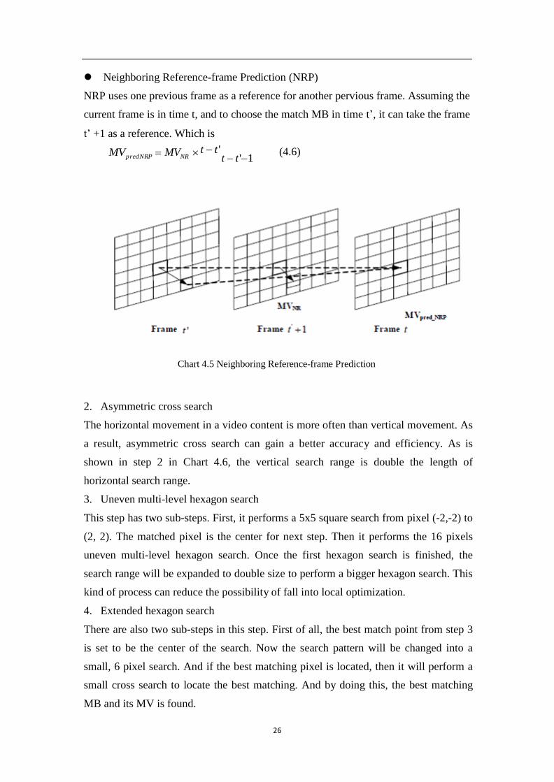
Neighboring Reference-frame Prediction (NRP)
NRP uses one previous frame as a reference for another pervious frame. Assuming the
current frame is in time t, and to choose the match MB in time t’, it can take the frame
t’ +1 as a reference. Which is
MVpredNRP MVNR t t ' t t '1
(4.6)
Chart 4.5 Neighboring Reference-frame Prediction
2. Asymmetric cross search
The horizontal movement in a video content is more often than vertical movement. As
a result, asymmetric cross search can gain a better accuracy and efficiency. As is
shown in step 2 in Chart 4.6, the vertical search range is double the length of
horizontal search range.
3. Uneven multi-level hexagon search
This step has two sub-steps. First, it performs a 5x5 square search from pixel (-2,-2) to
(2, 2). The matched pixel is the center for next step. Then it performs the 16 pixels
uneven multi-level hexagon search. Once the first hexagon search is finished, the
search range will be expanded to double size to perform a bigger hexagon search. This
kind of process can reduce the possibility of fall into local optimization.
4. Extended hexagon search
There are also two sub-steps in this step. First of all, the best match point from step 3
is set to be the center of the search. Now the search pattern will be changed into a
small, 6 pixel search. And if the best matching pixel is located, then it will perform a
small cross search to locate the best matching. And by doing this, the best matching
MB and its MV is found.
27
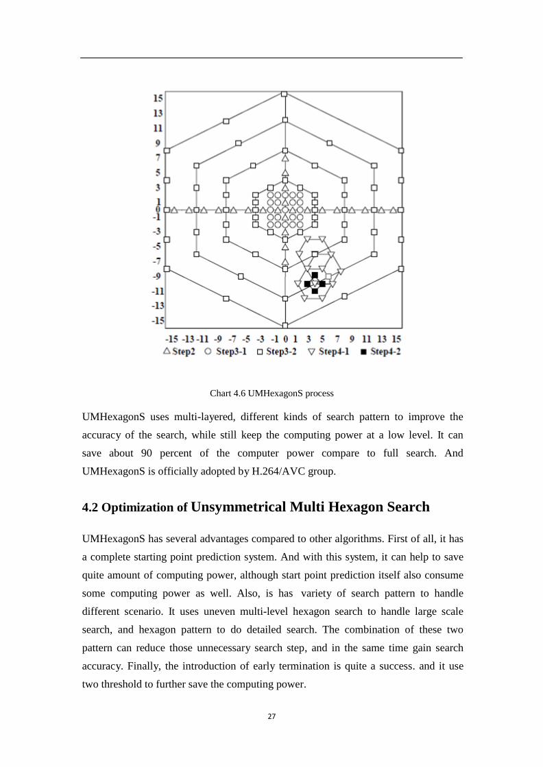
Chart 4.6 UMHexagonS process
UMHexagonS uses multi-layered, different kinds of search pattern to improve the
accuracy of the search, while still keep the computing power at a low level. It can
save about 90 percent of the computer power compare to full search. And
UMHexagonS is officially adopted by H.264/AVC group.
4.2 Optimization of Unsymmetrical Multi Hexagon Search
UMHexagonS has several advantages compared to other algorithms. First of all, it has
a complete starting point prediction system. And with this system, it can help to save
quite amount of computing power, although start point prediction itself also consume
some computing power as well. Also, is has variety of search pattern to handle
different scenario. It uses uneven multi-level hexagon search to handle large scale
search, and hexagon pattern to do detailed search. The combination of these two
pattern can reduce those unnecessary search step, and in the same time gain search
accuracy. Finally, the introduction of early termination is quite a success. and it use
two threshold to further save the computing power.
28
Because the advantages over other algorithms, this thesis uses UMHexagonS as the
model for further optimization. A good algorithm does not mean it is perfect in
every case, and after some deep thinking, this algorithms can be optimized in those
ways: First, UMHexagons is not specially made for mobile usage. Because the
quantization parameter (QP) in mobile usage is usually high, which means the
tolerance of the error is comparably high. As a result, some part of UMHexagons
is over designed. For example, after early termination, it still needs to do cross
search to locate the matching block. And here we can use the concept in
MVFAST "stop when good enough" to optimize the algorithm.
Secondly, for the threshold settings, UMHexagonS uses fixed value. Because the
video by nature is not static, and it can change beyond anyone's guess. It is not
reasonable to give a fixed number that can be adopted by all kinds of video.
Last, while the condition for early termination is met, in another word SAD is smaller
than threshold. Then we can consider the matching block is nearby and hexagon
search pattern is applied. But in several cases, for example the background is gradient
from black to dark grey, the left side of the image already meet the condition for early
termination. But the matching block is on the right side of the image. So it needs to
uses hexagon pattern to search from left to right, which will of course waste lots of
computing power. It is doubtable that SAD can be used to determine whether the
matching block is nearby.
To sum up those ideas, it is possible to further optimize UMHexagonS.
4.3 Optimization Details of Unsymmetrical Multi Hexagon
Search
4.3.1 Optimization on Early Termination
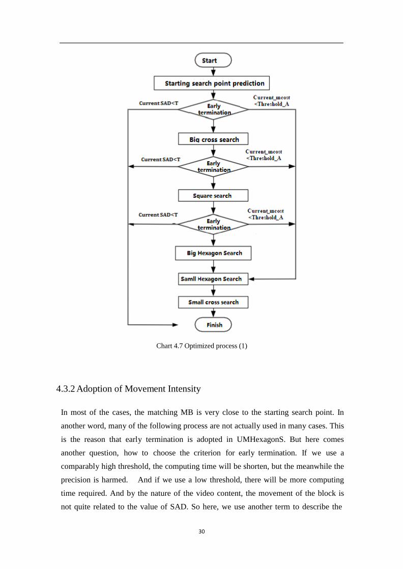
In UMHexagonS, two thresholds is applied for early termination, i.e. when the
predicted value is under the lower threshold, then the system consider this is the
perfect starting point and then perform small cross search. And if the value is under
the higher threshold, somehow higher than the lower threshold, system consider this is
an acceptable point, and then to perform hexagon search.
However, for a fast motion estimation algorithm, UMHexagonS is too complex on the
process. Because even the point can meet the criterion for early termination, it still
needs to perform hexagon search and small cross search, which are quite time
29
consuming.
Taking the core thought of MVFAST, stop when it is good enough, into consideration,
we change the details of early termination of UMHexagonS. The higher threshold is
kept untouched, while we change the lower threshold to acceptable threshold. Which
means if the predicted value is lower than the threshold, the whole search will come to
an end. And we can have the MV in the same time.
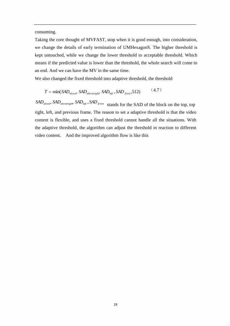
We also changed the fixed threshold into adaptive threshold, the threshold
T min( SADabove, SADaboveright, SADleft , SAD front ,512) (4.7)
SADabove, SADaboveright, SADleft , SAD front
stands for the SAD of the block on the top, top
right, left, and previous frame. The reason to set a adaptive threshold is that the video
content is flexible, and uses a fixed threshold cannot handle all the situations. With
the adaptive threshold, the algorithm can adjust the threshold in reaction to different
video content. And the improved algorithm flow is like this
30
Chart 4.7 Optimized process (1)
4.3.2 Adoption of Movement Intensity
In most of the cases, the matching MB is very close to the starting search point. In
another word, many of the following process are not actually used in many cases. This
is the reason that early termination is adopted in UMHexagonS. But here comes
another question, how to choose the criterion for early termination. If we use a
comparably high threshold, the computing time will be shorten, but the meanwhile the
precision is harmed. And if we use a low threshold, there will be more computing
time required. And by the nature of the video content, the movement of the block is
not quite related to the value of SAD. So here, we use another term to describe the
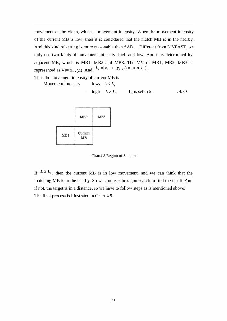
31
movement of the video, which is movement intensity. When the movement intensity
of the current MB is low, then it is considered that the match MB is in the nearby.
And this kind of setting is more reasonable than SAD. Different from MVFAST, we
only use two kinds of movement intensity, high and low. And it is determined by
adjacent MB, which is MB1, MB2 and MB3. The MV of MB1, MB2, MB3 is
represented as Vi=(xi , yi). And Li | xi | | yi |, L max( Li ) .
Thus the movement intensity of current MB is
Movement intensity = low, L L1
= high, L L1
L1 is set to 5. (4.8)
Chart4.8 Region of Support
If L L1 , then the current MB is in low movement, and we can think that the
matching MB is in the nearby. So we can uses hexagon search to find the result. And
if not, the target is in a distance, so we have to follow steps as is mentioned above.
The final process is illustrated in Chart 4.9.
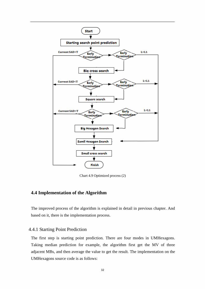
32
Chart 4.9 Optimized process (2)
4.4 Implementation of the Algorithm
The improved process of the algorithm is explained in detail in previous chapter. And
based on it, there is the implementation process.
4.4.1 Starting Point Prediction
The first step is starting point prediction. There are four modes in UMHexagons.
Taking median prediction for example, the algorithm first get the MV of three
adjacent MBs, and then average the value to get the result. The implementation on the
UMHexagons source code is as follows:
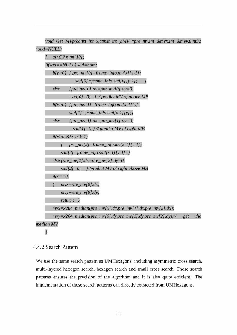
33
void Get_MVp(const int x,const int y,MV *pre_mv,int &mvx,int &mvy,uint32
*sad=NULL)
{ uint32 num[10];
if(sad==NULL) sad=num;
if(y>0) { pre_mv[0]=frame_info.mv[x][y-1];
sad[0]=frame_info.sad[x][y-1]; }
else {pre_mv[0].dx=pre_mv[0].dy=0;
sad[0]=0; } // predict MV of above MB
if(x>0) {pre_mv[1]=frame_info.mv[x-1][y];
sad[1]=frame_info.sad[x-1][y];}
else {pre_mv[1].dx=pre_mv[1].dy=0;
sad[1]=0;} // predict MV of right MB
if(x>0 && y<Y-1)
{ pre_mv[2]=frame_info.mv[x-1][y-1];
sad[2]=frame_info.sad[x-1][y-1]; }
else {pre_mv[2].dx=pre_mv[2].dy=0;
sad[2]=0; }//predict MV of right above MB
if(x==0)
{ mvx=pre_mv[0].dx;
mvy=pre_mv[0].dy;
return; }
mvx=x264_median(pre_mv[0].dx,pre_mv[1].dx,pre_mv[2] .dx);
mvy=x264_median(pre_mv[0].dy,pre_mv[1].dy,pre_mv[2].dy);// get the
median MV
}
4.4.2 Search Pattern
We use the same search pattern as UMHexagons, including asymmetric cross search,
multi-layered hexagon search, hexagon search and small cross search. Those search
patterns ensures the precision of the algorithm and it is also quite efficient. The
implementation of those search patterns can directly extracted from UMHexagons.
34
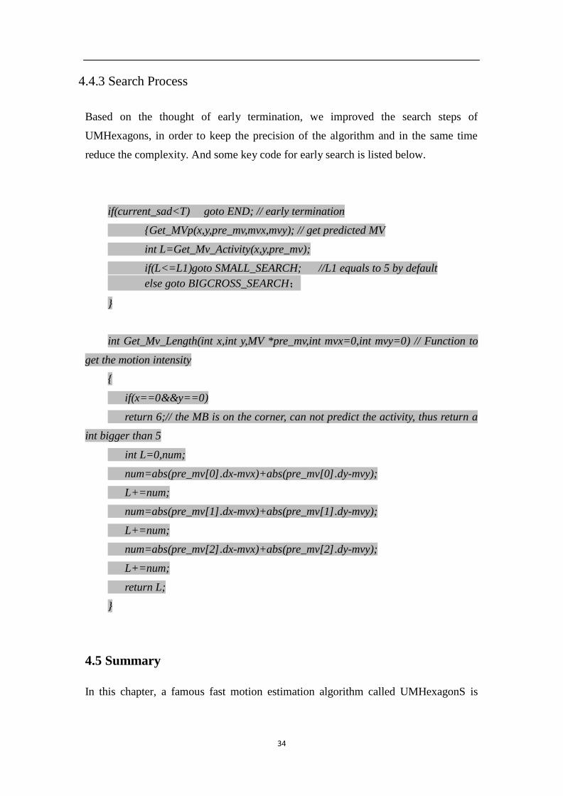
4.4.3 Search Process
Based on the thought of early termination, we improved the search steps of
UMHexagons, in order to keep the precision of the algorithm and in the same time
reduce the complexity. And some key code for early search is listed below.
if(current_sad<T) goto END; // early termination
{Get_MVp(x,y,pre_mv,mvx,mvy); // get predicted MV
int L=Get_Mv_Activity(x,y,pre_mv);
if(L<=L1)goto SMALL_SEARCH; //L1 equals to 5 by default
else goto BIGCROSS_SEARCH;
}
int Get_Mv_Length(int x,int y,MV *pre_mv,int mvx=0,int mvy=0) // Function to
get the motion intensity
{
if(x==0&&y==0)
return 6;// the MB is on the corner, can not predict the activity, thus return a
int bigger than 5
int L=0,num;
num=abs(pre_mv[0].dx-mvx)+abs(pre_mv[0].dy-mvy);
L+=num;
num=abs(pre_mv[1].dx-mvx)+abs(pre_mv[1].dy-mvy);
L+=num;
num=abs(pre_mv[2].dx-mvx)+abs(pre_mv[2].dy-mvy);
L+=num;
return L;
}
4.5 Summary
In this chapter, a famous fast motion estimation algorithm called UMHexagonS is

35
analyzed in detail. And based on its shorting comings, together with some thoughts in
other algorithms, this thesis provides some improvement and fully implementation.

36
37
Chapter 5 Experiment Proof of Improved Algorithm
Currently, there are two types of methodologies to evaluate the quality of video.
[18][19]They are Subjective Quality Assessment (SQA) and Objective Quality
Assessment (OQA). SQA uses a set of users to watch the video and give their ratings
objectively. On the contrast, OQA uses a scientific model to analysis the video and
then output some metric that can used to evaluate the quality of the video. In the
thesis, both methodologies are used to evaluate whether the optimized algorithms has
gain any improvement on video quality and coding efficiency.
5.1 Objective Quality Assessment based on JM Model
5.1.1 Design of the Experiment
JM Model [20] is developed by JVT team, as a reference model for H.264/AVC. This
model implements most of the key algorithms of H.264/AVC, and it is widely used
for scientific experiment.
The hardware of the computer used in this experiment has a CPU of Core2 1.8Ghz. It
has a memory of 2 gigabytes and also a 7200rpm hard disk. The OS is windows 7 and
JM model version is 17.2. And the IDE is visual studio 2008.
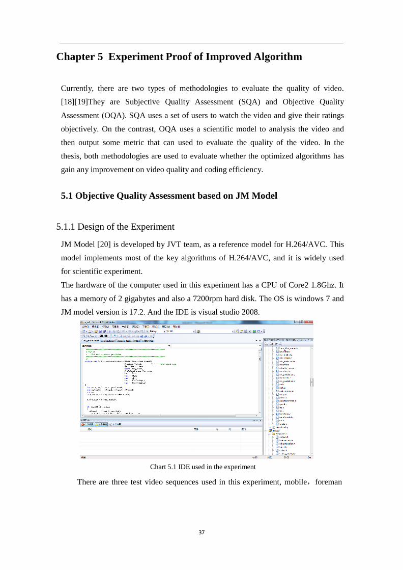
Chart 5.1 IDE used in the experiment
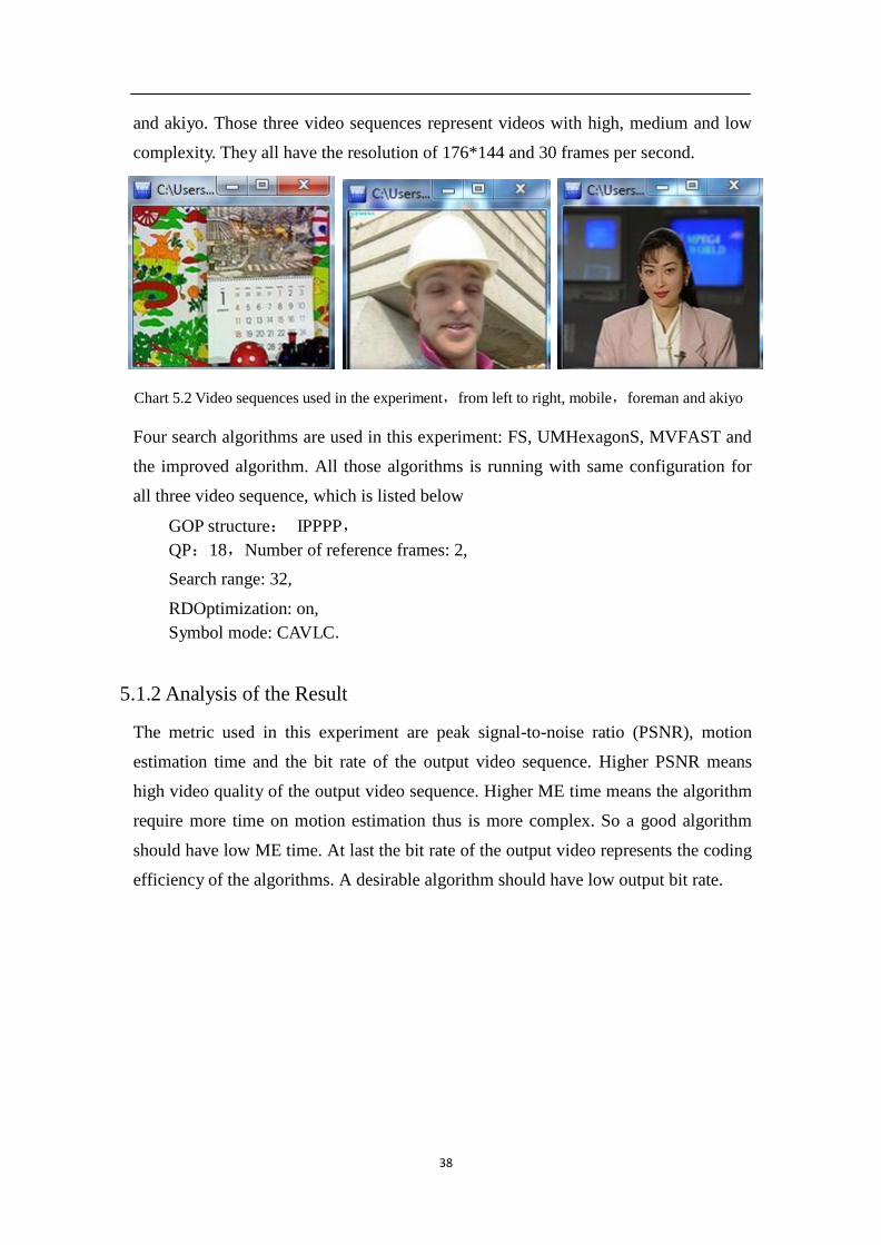
There are three test video sequences used in this experiment, mobile,foreman
38
and akiyo. Those three video sequences represent videos with high, medium and low
complexity. They all have the resolution of 176*144 and 30 frames per second.
Chart 5.2 Video sequences used in the experiment,from left to right, mobile,foreman and akiyo
Four search algorithms are used in this experiment: FS, UMHexagonS, MVFAST and
the improved algorithm. All those algorithms is running with same configuration for
all three video sequence, which is listed below
GOP structure: IPPPP,
QP:18,Number of reference frames: 2,
Search range: 32,
RDOptimization: on,
Symbol mode: CAVLC.
5.1.2 Analysis of the Result
The metric used in this experiment are peak signal-to-noise ratio (PSNR), motion
estimation time and the bit rate of the output video sequence. Higher PSNR means
high video quality of the output video sequence. Higher ME time means the algorithm
require more time on motion estimation thus is more complex. So a good algorithm
should have low ME time. At last the bit rate of the output video represents the coding
efficiency of the algorithms. A desirable algorithm should have low output bit rate.
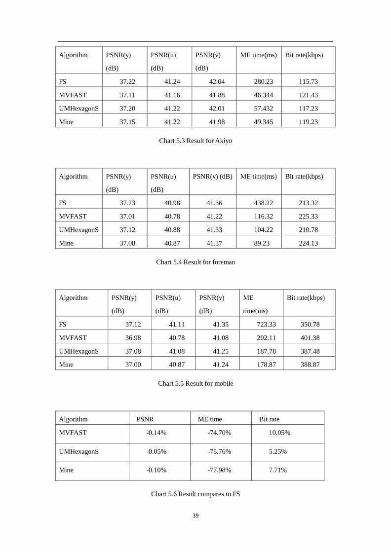
39
Algorithm
PSNR(y)
(dB)
PSNR(u)
(dB)
PSNR(v)
(dB)
ME time(ms)
Bit rate(kbps)
FS
37.22
41.24
42.04
280.23
115.73
MVFAST
37.11
41.16
41.88
46.344
121.43
UMHexagonS
37.20
41.22
42.01
57.432
117.23
Mine
37.15
41.22
41.98
49.345
119.23
Chart 5.3 Result for Akiyo
Algorithm PSNR(y)
(dB)
PSNR(u)
(dB)
PSNR(v) (dB)
ME time(ms)
Bit rate(kbps)
FS
37.23
40.98
41.36
438.22
213.32
MVFAST
37.01
40.78
41.22
116.32
225.33
UMHexagonS
37.12
40.88
41.33
104.22
210.78
Mine
37.08
40.87
41.37
89.23
224.13
Chart 5.4 Result for foreman
Algorithm
PSNR(y)
(dB)
PSNR(u)
(dB)
PSNR(v)
(dB)
ME
time(ms)
Bit rate(kbps)
FS
37.12
41.11
41.35
723.33
350.78
MVFAST
36.98
40.78
41.08
202.11
401.38
UMHexagonS
37.08
41.08
41.25
187.78
387.48
Mine
37.00
40.87
41.24
178.87
388.87
Chart 5.5 Result for mobile
Algorithm
PSNR
ME time
Bit rate
MVFAST
-0.14%
-74.70%
10.05%
UMHexagonS
-0.05%
-75.76%
5.25%
Mine
-0.10%
-77.98%
7.71%
Chart 5.6 Result compares to FS
40
From the result we can see that MVFAST UMHexagonS and the improved algorithms
all has significant advantage compared to FS, especially in the Akiyo sequence with
lowest complexity. Those three only require one fifth of the time to finish the motion
estimation. As the video complexity goes up, the gap is closing up, but still in the
highest complexity video sequence Mobile, the ratio is one to three. And comparing
within those three algorithms, the improved algorithms has the lowest ME time,
having 10 percent advantage comparing to UMHexagonS.
On the term of PSNR, FS is no doubt the best, because all the possible block are
precisely calculated. Compare to FS, all the other algorithms has a margin from 0.1bB
to 0.2dB. And the PSNR of the improved algorithm is slightly lower than
UMHexagonS, better than MVFAST. And the result is reasonable, because some of
the step are cut in UMHexagonS.
The result is similar for output bit rate. All the three algorithms has 5kpbs to 15kpbs
shift comparing to FS. But this margin is not significant for video sequence.
From chart 4, we can see more obviously that the improved algorithm has the lowest
ME time, saving 77.98% of the ME time required by FS. And its PSNR is better than
MVFAST, slightly lower than UMHexagonS. In another way, we can say that the
improved algorithm saves 2.2% of algorithms complexity, and in return only sacrifice
0.5% of the video quality compared to UMHexagonS.
5.2 Subjective Quality Assessment Using Double Stimulus
Impairment Scale
5.2.1 Design of Experiment
Double Stimulus Impairment Scale is used in the experiment, the participator will
watch a video sequence, coupled by the original video sequence and the output
sequence. And then give rating on the difference between those two sequences. There
are five scales used here
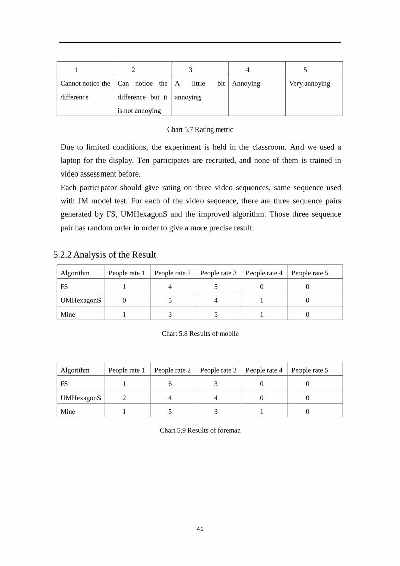
41
1
2
3
4
5
Cannot notice the
difference
Can notice the
difference but it
is not annoying
A little bit
annoying
Annoying
Very annoying
Chart 5.7 Rating metric
Due to limited conditions, the experiment is held in the classroom. And we used a
laptop for the display. Ten participates are recruited, and none of them is trained in
video assessment before.
Each participator should give rating on three video sequences, same sequence used
with JM model test. For each of the video sequence, there are three sequence pairs
generated by FS, UMHexagonS and the improved algorithm. Those three sequence
pair has random order in order to give a more precise result.
5.2.2 Analysis of the Result
Algorithm
People rate 1
People rate 2
People rate 3
People rate 4
People rate 5
FS
1
4
5
0
0
UMHexagonS
0
5
4
1
0
Mine
1
3
5
1
0
Chart 5.8 Results of mobile
Algorithm
People rate 1
People rate 2
People rate 3
People rate 4
People rate 5
FS
1
6
3
0
0
UMHexagonS
2
4
4
0
0
Mine
1
5
3
1
0
Chart 5.9 Results of foreman
42
Algorithm
People rate 1
People rate 2
People rate 3
People rate 4
People rate 5
FS
5
4
1
0
0
UMHexagonS
5
2
2
1
0
Mine
6
3
1
0
0
Chart 5.10 Results of akiyo
Algorithm
Mobile
Foreman
Akiyo
All
FS
2.4
2.2
1.6
2.07
UMHexagonS
2.6
2.2
1.9
2.23
Mine
2.9
2.4
1.5
2.27
Chart 5.11 Results of average rating
The result shows that the improved algorithm does not have significant video quality
reduction comparing to the most complicated algorithm, FS. And it even surpasses FS
in Akiyo sequence. (Of course there is some subjective deviation) For the average
score, the improved algorithm is 2.27, only 0.04 behind UMHexagonS. And it can
conclude that the improved algorithm does not have obvious reduction on video
quality compare to UMHexagonS, especially on video with low complexity. So for
the application like video chat that only has low video complexity, this algorithm can
gain more advantages.
5.3 Summary
In this chapter, both Objective Quality Assessment and Subjective Quality
Assessment are used to evaluate the performance of the improved algorithms. In OQA,
JM Model is used as a test platform to evaluate three major metrics of video coding
performance. In SQA, DISS is adopted. And both experiments show that the
improved algorithms can reduce the complexity of the motion estimation while in the
same time keep the video quality unharmed. And this improved algorithm is suitable
for 3G usage.
43
Chapter 6 Conclusion
The application of video content over 3G network relies heavily on the video codec.
Because video codec can impact the clarity, file size, real timing of the video content.
As the most resource-consuming part of the video coding process, Motion estimation
is considered to be the bottom neck of the whole process. So this thesis focus on the
motion estimation algorithm, more precisely, block-based motion estimation
algorithm. It researches into the core technology and the framework of H.264/AVC.
And then compares the pros and cons of some classic motion estimation algorithms,
from which pick the most outstanding algorithm, UMHexagonS as the target for
further optimization. Under deep analysis and thinking, some shortcoming of
UMHexagonS is found and conquered, and also some of the classic thoughts are
brought into the new, improved algorithms. And in the end, both OQA and SQA are
used in the evaluation of coding performance of the improved algorithm. The result
shows that the improved algorithms can reduce the complexity of the motion
estimation while in the same time keep the video quality unharmed. And this
algorithm can be quite suitable for 3G network usage.
44
References
[1] Richardson I E. The H. 264 advanced video compression standard [M]. Wiley, 2011.
[2] Richardson I E G. H. 264/MPEG-4 Part 10: Transform & Quantization [J]. A white paper.
[Online]. Available: http://www. vcodex. com, 2003.
[3] Richardson I E G. H. 264/MPEG-4 Part 10 White Paper: Overview of H. 264[J]. Oct, 2002, 7:
1-3.
[4] Bo Li, Recent advances on TD-SCDMA in China, Communications Magazine, IEEE, Volume
43, Issue: 1 Page 30 – 37
[5] Agrawal, P., Battery power sensitive video processing in wireless networks, Personal, Indoor
and Mobile Radio Communications, 1998. The Ninth IEEE International Symposium on,
116- 120 vol.1
[6] Tuan, J.-C. Chang, T.-S. Jen, C.-W, On the Data Reuse and Memory Bandwidth Analysis for
Full-Search Block-Matching VLSI Architecture, IEEE TRANSACTIONS ON CIRCUITS
AND SYSTEMS FOR VIDEO TECHNOLOGY, 2002, VOL 12; PART 1, pages 61-72
[7] Jong, H.-M. Chen, L.-G. Chiueh, T.-D., Accuracy Improvement and Cost Reduction of 3-Step
Search Block Matching Algorithm for Video Coding, INSTITUTEOF ELECTRICAL AND
ELECTRONICS ENGINEERS,1994, VOL 4; NUMBER 1, pages 88
[8] Li, R. Zeng, B. Liou, M. L.,A New Three-Step Search Algorithm for Block Motion
Estimation,INSTITUTEOF ELECTRICAL AND ELECTRONICS ENGINEERS,1994, VOL
4; NUMBER 4, pages 438
[9] Po, L.-M. Ma, W.-C., A Novel Four-Step Search Algorithm for Fast Block Motion Estimation,
INSTITUTEOF ELECTRICAL AND ELECTRONICS ENGINEERS, 1996, VOL 6;
NUMBER 3, pages 313-316
[10] Liu, L.-K. Feig, E., A Block-Based Gradient Descent Search Algorithm for Block Motion
Estimation in Video Coding, INSTITUTEOF ELECTRICAL AND ELECTRONICS
ENGINEERS, 1996, VOL 6; NUMBER 4, pages 419-421
[11] Chen, O. T.-C., Motion Estimation Using a One-Dimensional Gradient Descent Search, IEEE
TRANSACTIONS ON CIRCUITS AND SYSTEMS FOR VIDEO TECHNOLOGY, 2000,
VOL 10; PART 4, pages 608-616
[12] Zhu, S. Ma, K. K., A New Diamond Search Algorithm for Fast Block-Matching Motion,
IEEE TRANSACTIONS ON IMAGE PROCESSING, 2000, VOL 9; PART 2, pages 287-290
[13] Zhu, C. Lin, X. Chau, L.-P., Hexagon-Based Search Pattern for Fast Block Motion Estimation,
INSTITUTEOF ELECTRICAL AND ELECTRONICS ENGINEERS, 2002, VOL 12; PART
5, pages 349-355
[14] Tourapis, A. M. Au, O. C. Liou, M. L., Predictive motion vector field adaptive search
technique (PMVFAST): enhancing block-based motion estimation [4310-92],
PROCEEDINGS- SPIE THE INTERNATIONAL SOCIETY FOR OPTICAL
ENGINEERING, 2001, ISSU 4310, pages 883-892
[15] Nicolas, Henri, and Claude Labit. "Region-based motion estimation using deterministic
relaxation schemes for image sequence coding." Acoustics, Speech, and Signal Processing,
45
1992. ICASSP-92., 1992 IEEE International Conference on. Vol. 3. IEEE, 1992.
[16] Chen, Mei-Juan, et al. "A new block-matching criterion for motion estimation and its
implementation." Circuits and Systems for Video Technology, IEEE Transactions on 5.3
(1995): 231-236.
[17] CA Rahman, W Badawy, UMHexagonS algorithm based motion estimation architecture for H.
264/AVC, System-on-Chip for Real-Time, 2005 .
[18] Wang, Zhou, et al. "Image quality assessment: From error visibility to structural
similarity." Image Processing, IEEE Transactions on 13.4 (2004): 600-612.
[19] Huynh-Thu, Quan, and Mohammed Ghanbari. "Scope of validity of PSNR in image/video
quality assessment." Electronics letters 44.13 (2008): 800-801.
[20] H.264/AVC reference software JM17.2, http://iphome.hhi.de/suehring/tml, 2010
Related Documents