Sparse Signal Estimation by Maximally Sparse Convex Optimization

IEEE TRANSACTIONS ON SIGNAL PROCESSING. 2014 (PREPRINT) 1

Sparse Signal Estimation by Maximally SparseConvex Optimization

Ivan W. Selesnick and Ilker Bayram

Abstract—This paper addresses the problem of sparsity penal-ized least squares for applications in sparse signal processing,e.g. sparse deconvolution. This paper aims to induce sparsitymore strongly than L1 norm regularization, while avoiding non-convex optimization. For this purpose, this paper describes thedesign and use of non-convex penalty functions (regularizers)constrained so as to ensure the convexity of the total cost function,F, to be minimized. The method is based on parametric penaltyfunctions, the parameters of which are constrained to ensureconvexity of F. It is shown that optimal parameters can beobtained by semidefinite programming (SDP). This maximallysparse convex (MSC) approach yields maximally non-convexsparsity-inducing penalty functions constrained such that thetotal cost function, F, is convex. It is demonstrated that iterativeMSC (IMSC) can yield solutions substantially more sparse thanthe standard convex sparsity-inducing approach, i.e., L1 normminimization.

I. INTRODUCTION

In sparse signal processing, the `1 norm has special sig-nificance [4], [5]. It is the convex proxy for sparsity. Giventhe relative ease with which convex problems can be reli-ably solved, the `1 norm is a basic tool in sparse signalprocessing. However, penalty functions that promote sparsitymore strongly than the `1 norm yield more accurate results inmany sparse signal estimation/reconstruction problems. Hence,numerous algorithms have been devised to solve non-convexformulations of the sparse signal estimation problem. In thenon-convex case, generally only a local optimal solution canbe ensured; hence solutions are sensitive to algorithmic details.

This paper aims to develop an approach that promotessparsity more strongly than the `1 norm, but which attempts toavoid non-convex optimization as far as possible. In particular,the paper addresses ill-posed linear inverse problems of theform

arg minx∈RN

{F (x) = ‖y −Hx‖22 +

N−1∑

n=0

λnφn(xn)}

(1)

where λn > 0 and φn : R → R are sparsity-inducingregularizers (penalty functions) for n ∈ ZN = {0, . . . , N−1}.Problems of this form arise in denoising, deconvolution,

Copyright (c) 2013 IEEE. Personal use of this material is permitted.However, permission to use this material for any other purposes must beobtained from the IEEE by sending a request to [email protected].

I. W. Selesnick is with the Department of Electrical and Computer Engineer-ing, NYU Polytechnic School of Engineering, 6 Metrotech Center, Brooklyn,NY 11201, USA. Email: [email protected]. I. Bayram is with the Departmentof Electronics and Communication Engineering, Istanbul Technical University,Maslak, 34469, Istanbul, Turkey. Email: [email protected].

This research was support by the NSF under Grant No. CCF-1018020.

compressed sensing, etc. Specific motivating applications in-clude nano-particle detection for bio-sensing and near infraredspectroscopic time series imaging [61], [62].

This paper explores the use of non-convex penalty functionsφn, under the constraint that the total cost function F is convexand therefore reliably minimized. This idea, introduced byBlake and Zimmerman [6], is carried out

. . . by balancing the positive second derivatives inthe first term [quadratic fidelity term] against thenegative second derivatives in the [penalty] terms[6, page 132].

This idea is also proposed by Nikolova in Ref. [49] where it isused in the denoising of binary images. In this work, to carryout this idea, we employ penalty functions parameterized byvariables an, i.e., φn(x) = φ(x; an), wherein the parametersan are selected so as to ensure convexity of the total costfunction F . We note that in [6], the proposed family of penaltyfunctions are quadratic around the origin and that all an areequal. On the other hand, the penalty functions we utilize inthis work are non-differentiable at the origin as in [52], [54](so as to promote sparsity) and the an are not constrained tobe equal.

A key idea is that the parameters an can be optimizedto make the penalty functions φn maximally non-convex(i.e., maximally sparsity-inducing), subject to the constraintthat F is convex. We refer to this as the ‘maximally-sparseconvex’ (MSC) approach. In this paper, the allowed intervalfor the parameters an, to ensure F is convex, is obtained byformulating a semidefinite program (SDP) [2], which is itselfa convex optimization problem. Hence, in the proposed MSCapproach, the cost function F to be minimized depends itselfon the solution to a convex problem. This paper also describesan iterative MSC (IMSC) approach that boosts the applicabilityand effectiveness of the MSC approach. In particular, IMSCextends MSC to the case where H is rank deficient or illconditioned; e.g., overcomplete dictionaries and deconvolutionof near singular systems.

The proposed MSC approach requires a suitable parametricpenalty function φ(· ; a), where a controls the degree to whichφ is non-convex. Therefore, this paper also addresses thechoice of parameterized non-convex penalty functions so asto enable the approach. The paper proposes suitable penaltyfunctions φ and describes their relevant properties.

A. Related Work (Threshold Functions)

When H in (1) is the identity operator, the problem is one ofdenoising and is separable in xn. In this case, a sparse solution

arX

iv:1

302.

5729

v3 [

cs.L

G]

3 J

an 2

014

2 IEEE TRANSACTIONS ON SIGNAL PROCESSING. 2014 (PREPRINT)

x is usually obtained by some type of threshold function,θ : R → R. The most widely used threshold functions arethe soft and hard threshold functions [21]. Each has its disad-vantages, and many other thresholding functions that providea compromise of the soft and hard thresholding functionshave been proposed – for example: the firm threshold [32],the non-negative (nn) garrote [26], [31], the SCAD thresholdfunction [24], [73], and the proximity operator of the `p quasi-norm (0 < p < 1) [44]. Several penalty functions are unifiedby the two-parameter formulas given in [3], [35], whereinthreshold functions are derived as proximity operators [19].(Table 1.2 of [19] lists the proximity operators of numerousfunctions.) Further threshold functions are defined directly bytheir functional form [70]–[72].

Sparsity-based nonlinear estimation algorithms can also bedeveloped by formulating suitable non-Gaussian probabilitymodels that reflect sparse behavior, and by applying Bayesianestimation techniques [1], [17], [23], [39], [40], [48], [56].We note that, the approach we take below is essentially adeterministic one; we do not explore its formulation from aBayesian perspective.

This paper develops a specific threshold function designedso as to have the three properties advocated in [24]: unbiased-ness (of large coefficients), sparsity, and continuity. Further,the threshold function θ and its corresponding penalty functionφ are parameterized by two parameters: the threshold T andthe right-sided derivative of θ at the threshold, i.e. θ′(T+),a measure of the threshold function’s sensitivity. Like otherthreshold functions, the proposed threshold function biaseslarge |xn| less than does the soft threshold function, but iscontinuous unlike the hard threshold function. As will beshown below, the proposed function is most similar to thethreshold function (proximity operator) corresponding to thelogarithmic penalty, but it is designed to have less bias. It isalso particularly convenient in algorithms for solving (1) thatdo not call on the threshold function directly, but instead callon the derivative of penalty function, φ′(x), due to its simplefunctional form. Such algorithms include iterative reweightedleast squares (IRLS) [38], iterative reweighted `1 [11], [69],FOCUSS [58], and algorithms derived using majorization-minimization (MM) [25] wherein the penalty function is upperbounded (e.g. by a quadratic or linear function).

B. Related Work (Sparsity Penalized Least Squares)Numerous problem formulations and algorithms to obtain

sparse solutions to the general ill-posed linear inverse problem,(1), have been proposed. The `1 norm penalty (i.e., φn(x) =|x|) has been proposed for sparse deconvolution [10], [16],[41], [66] and more generally for sparse signal processing [15]and statistics [67]. For the `1 norm and other non-differentiableconvex penalties, efficient algorithms for large scale problemsof the form (1) and similar (including convex constraints)have been developed based on proximal splitting methods [18],[19], alternating direction method of multipliers (ADMM) [9],majorization-minimization (MM) [25], primal-dual gradientdescent [22], and Bregman iterations [36].

Several approaches aim to obtain solutions to (1) that aremore sparse than the `1 norm solution. Some of these methods

proceed first by selecting a non-convex penalty function thatinduces sparsity more strongly than the `1 norm, and second bydeveloping non-convex optimization algorithms for the mini-mization of F ; for example, iterative reweighted least squares(IRLS) [38], [69], FOCUSS [37], [58], extensions thereof [47],[65], half-quadratic minimization [12], [34], graduated non-convexity (GNC) [6], and its extensions [50]–[52], [54].

The GNC approach for minimizing a non-convex function Fproceeds by minimizing a sequence of approximate functions,starting with a convex approximation of F and ending withF itself. While GNC was originally formulated for imagesegmentation with smooth penalties, it has been extended togeneral ill-posed linear inverse problems [51] and non-smoothpenalties [46], [52], [54].

With the availability of fast reliable algorithms for `1norm minimization, reweighted `1 norm minimization is asuitable approach for the non-convex problem [11], [69]: thetighter upper bound of the non-convex penalty provided bythe weighted `1 norm, as compared to the weighted `2 norm,reduces the chance of convergence to poor local minima. Otheralgorithmic approaches include ‘difference of convex’ (DC)programming [33] and operator splitting [13].

In contrast to these works, in this paper the penalties φnare constrained by the operator H and by λn. This approach(MSC) deviates from the usual approach wherein the penaltyis chosen based on prior knowledge of x. We also notethat, by design, the proposed approach leads to a convexoptimization problem; hence, it differs from approaches thatpursue non-convex optimization. It also differs from usualconvex approaches for sparse signal estimation/recovery whichutilize convex penalties. In this paper, the aim is precisely toutilize non-convex penalties that induce sparsity more stronglythan a convex penalty possibly can.

The proposed MSC approach is most similar to the gen-eralizations of GNC to non-smooth penalties [50], [52], [54]that have proven effective for the fast image reconstructionwith accurate edge reproduction. In GNC, the convex approx-imation of F is based on the minimum eigenvalue of HTH.The MSC approach is similar but more general: not all an areequal. This more general formulation leads to an SDP, not aneigenvalue problem. In addition, GNC comprises a sequenceof non-convex optimizations, whereas the proposed approach(IMSC) leads to a sequence of convex problems. The GNCapproach can be seen as a continuation method, wherein aconvex approximation of F is gradually transformed to F ina predetermined manner. In contrast, in the proposed approach,each optimization problem is defined by the output of an SDPwhich depends on the support of the previous solution. In asense, F is redefined at each iteration, to obtain progressivelysparse solutions.

By not constraining all an to be equal, the MSC approachallows a more general parametric form for the penalty, andas such, it can be more non-convex (i.e., more sparsitypromoting) than if all an are constrained to be equal. Theexample in Sec. III-F compares the two cases (with andwithout the simplification that all an are equal) and shows thatthe simplified version gives inferior results. (The simplifiedform is denoted IMSC/S in Table I and Fig. 9 below).

3

If the measurement matrix H is rank deficient, and if allan were constrained to be equal, then the only solution inthe proposed approach would have an = 0 for all n; i.e.,the penalty function would be convex. In this case, it is notpossible to gain anything by allowing the penalty functionto be non-convex subject to the constraint that the total costfunction is convex. On the other hand, the proposed MSCapproach, depending on H, can still have all or some an > 0and hence can admit non-convex penalties (in turn, promotingsparsity more strongly).L0 minimizaton: A distinct approach to obtain sparse solu-tions to (1) is to find an approximate solution minimizing the`0 quasi-norm or satisfying an `0 constraint. Examples of suchalgorithms include: matching pursuit (MP) and orthogonal MP(OMP) [45], greedy `1 [43], iterative hard thresholding (IHT)[7], [8], [42], [55], hard thresholding pursuit [28], smoothed`0, [46], iterative support detection (ISD) [68], single bestreplacement (SBR) [63], and ECME thresholding [57].

Compared to algorithms aiming to solve the `0 quasi-normproblem, the proposed approach again differs. First, the `0problem is highly non-convex, while the proposed approachdefines a convex problem. Second, methods for `0 seek thecorrect support (index set of non-zero elements) of x anddo not regularize (penalize) any element xn in the calculatedsupport. In contrast, the design of the regularizer (penalty)is at the center of the proposed approach, and no xn is leftunregularized.

II. SCALAR THRESHOLD FUNCTIONS

The proposed threshold function and corresponding penaltyfunction is intended to serve as a compromise between softand hard threshold functions, and as a parameterized familyof functions for use with the proposed MSC method for ill-posed linear inverse problems, to be described in Sect. III.

First, we note the high sensitivity of the hard thresholdfunction to small changes in its input. If the input is slightlyless than the threshold T , then a small positive perturbationproduces a large change in the output, i.e., θh(T − ε) = 0and θh(T + ε) ≈ T where θh : R → R denotes the hardthreshold function. Due to this discontinuity, spurious noisepeaks/bursts often appear as a result of hard-thresholdingdenoising. For this reason, a continuous threshold functionis often preferred. The susceptibility of a threshold functionθ to the phenomenon of spurious noise peaks can be roughlyquantified by the maximum value its derivative attains, i.e.,maxy∈R θ

′(y), provided θ is continuous. For the thresholdfunctions considered below, θ′ attains its maximum valueat y = ±T+; hence, the value of θ′(T+) will be noted.The soft threshold function θs has θ′s(T

+) = 1 reflectingits insensitivity. However, θs substantially biases (attenuates)large values of its input; i.e., θs(y) = y − T for y > T .

A. Problem Statement

In this section, we seek a threshold function and correspond-ing penalty (i) for which the ‘sensitivity’ θ′(T+) can be readilytuned from 1 to infinity and (ii) that does not substantially biaslarge y, i.e., y − θ(y) decays to zero rapidly as y increases.

For a given penalty function φ, the proximity operator [19]denoted θ : R→ R is defined by

θ(y) = argminx∈R

{F (x) =

1

2(y − x)2 + λφ(x)

}(2)

where λ > 0. For uniqueness of the minimizer, we assumein the definition of θ(y) that F is strictly convex. Commonsparsity-inducing penalties include

φ(x) = |x| and φ(x) =1

alog(1 + a |x|). (3)

We similarly assume in the following that φ(x) is three timescontinuously differentiable for all x ∈ R except x = 0, andthat φ is symmetric, i.e., φ(−x) = φ(x).

If θ(y) = 0 for all |y| 6 T for some T > 0, and T isthe maximum such value, then the function θ is a thresholdfunction and T is the threshold.

It is often beneficial in practice if θ admits a simple func-tional form. However, as noted above, a number of algorithmsfor solving (1) do not use θ directly, but use φ′ instead. In thatcase, it is beneficial if φ′ has a simple function form. This isrelevant in Sec. III where such algorithms will be used.

In order that y−θ(y) approaches zero, the penalty functionφ must be non-convex, as shown by the following.

Proposition 1. Suppose φ : R→ R is a convex function andθ(y) denotes the proximity operator associated with φ, definedin (2). If 0 6 y1 6 y2, then

y1 − θ(y1) 6 y2 − θ(y2). (4)

Proof: Let ui = θ(yi) for i = 1, 2. We have,

yi ∈ ui + λ∂φ(ui). (5)

Since y2 > y1, by the monotonicity of both of the terms onthe right hand side of (5), it follows that u2 > u1.

If u2 = u1, (4) holds with since y2 ≥ y1.Suppose now that u2 > u1. Note that the subdifferential

∂φ is also a monotone mapping since φ is a convex function.Therefore it follows that if zi ∈ λ∂φ(ui), we should havez2 > z1. Since yi − θ(yi) ∈ λ∂φ(ui), the claim follows.

According to the proposition, if the penalty is convex, thenthe gap between θ(y) and y increases as the magnitude of yincreases. The larger y is, the greater the bias (attenuation)is. The soft threshold function is an extreme case that keepsthis gap constant (beyond the threshold T , the gap is equal toT ). Hence, in order to avoid attenuation of large values, thepenalty function must be non-convex.

B. Properties

As detailed in the Appendix, the proximity operator (thresh-old function) θ defined in (2) can be expressed as

θ(y) =

{0, |y| ≤ Tf−1(y), |y| ≥ T (6)

where the threshold, T , is given by

T = λφ′(0+) (7)

4 IEEE TRANSACTIONS ON SIGNAL PROCESSING. 2014 (PREPRINT)

and f : R+ → R is defined as

f(x) = x+ λφ′(x). (8)

As noted in the Appendix, F is strictly convex if

φ′′(x) > − 1

λ, ∀x > 0. (9)

In addition, we have

θ′(T+) =1

1 + λφ′′(0+)(10)

andθ′′(T+) = − λφ′′′(0+)

[1 + λφ′′(0+)]3. (11)

Equations (10) and (11) will be used in the following. Asnoted above, θ′(T+) reflects the maximum sensitivity of θ.The value θ′′(T+) is also relevant; it will be set in Sec. II-Dso as to induce θ(y)− y to decay rapidly to zero.

C. The Logarithmic Penalty Function

The logarithmic penalty function can be used for the MSCmethod to be described in Sec. III. It also serves as the modelfor the penalty function developed in Sec. II-D below, designedto have less bias. The logarithmic penalty is given by

φ(x) =1

alog(1 + a |x|), 0 < a ≤ 1

λ(12)

which is differentiable except at x = 0. For x 6= 0, thederivative of φ is given by

φ′(x) =1

1 + a |x| sign(x), x 6= 0, (13)

as illustrated in Fig. 1a. The function f(x) = x + λφ′(x) isillustrated in Fig. 1b. The threshold function θ, given by (6),is illustrated in Fig. 1c.

Let us find the range of a for which F is convex. Note that

φ′′(x) = − a

(1 + ax)2, φ′′′(x) =

2a2

(1 + ax)3

for x > 0. Using the condition (9), it is deduced that if 0 <a ≤ 1/λ, then f(x) is increasing, the cost function F in (2)is convex, and the threshold function θ is continuous.

Using (7), the threshold is given by T = λ. To find θ′(T+)and θ′′(T+), note that φ′′(0+) = −a, and φ′′′(0+) = 2a2.Using (10) and (11), we then have

θ′(T+) =1

1− aλ, θ′′(T+) = − 2a2λ

(1− aλ)3 . (14)

As a varies between 0 and 1/λ, the derivative θ′(T+) variesbetween 1 and infinity. As a approaches zero, θ approaches thesoft-threshold function. We can set a so as to specify θ′(T+).Solving (14) for a gives

a =1

λ

(1− 1

θ′(T+)

). (15)

Therefore, T and θ′(T+) can be directly specified by settingthe parameters λ and a (i.e., λ = T and a is given by (15)).

Note that θ′′(T+) given in (14) is strictly negative exceptwhen a = 0 which corresponds to the soft threshold function.

4

and f : R+ ! R is defined as

f(x) = x + ��0(x). (8)

As noted in the Appendix, F is strictly convex if

�00(x) > � 1

�, 8x > 0. (9)

In addition, we have

✓0(T+) =1

1 + ��00(0+)(10)

and✓00(T+) = � ��000(0+)

[1 + ��00(0+)]3. (11)

Equations (10) and (11) will be used in the following. Asnoted above, ✓0(T+) reflects the maximum sensitivity of ✓.The value ✓00(T+) is also relevant; it will be set in Sec. II-Dso as to induce ✓(y) � y to decay rapidly to zero.

C. The Logarithmic Penalty Function

The logarithmic penalty function can be used for the MSCmethod to be described in Sec. III. It also serves as the modelfor the penalty function developed in Sec. II-D below, designedto have less bias. The logarithmic penalty is given by

�(x) =1

alog(1 + a |x|), 0 < a 1

�(12)

which is differentiable except at x = 0. For x 6= 0, thederivative of � is given by

�0(x) =1

1 + a |x| sign(x), x 6= 0, (13)

as illustrated in Fig. 1a. The function f(x) = x + ��0(x) isillustrated in Fig. 1b. The threshold function ✓, given by (6),is illustrated in Fig. 1c.

Let us find the range of a for which F is convex. Note that

�00(x) = � a

(1 + ax)2, �000(x) =

2a2

(1 + ax)3

for x > 0. Using the condition (9), it is deduced that if 0 <a 1/�, then f(x) is increasing, the cost function F in (2)is convex, and the threshold function ✓ is continuous.

Using (7), the threshold is given by T = �. To find ✓0(T+)and ✓00(T+), note that �00(0+) = �a, and �000(0+) = 2a2.Using (10) and (11), we then have

✓0(T+) =1

1 � a�, ✓00(T+) = � 2a2�

(1 � a�)3. (14)

As a varies between 0 and 1/�, the derivative ✓0(T+) variesbetween 1 and infinity. As a approaches zero, ✓ approaches thesoft-threshold function. We can set a so as to specify ✓0(T+).Solving (14) for a gives

a =1

�

✓1 � 1

✓0(T+)

◆. (15)

Therefore, T and ✓0(T+) can be directly specified by settingthe parameters � and a (i.e., � = T and a is given by (15)).

Note that ✓00(T+) given in (14) is strictly negative exceptwhen a = 0 which corresponds to the soft threshold function.

!10 !5 0 5 10!2

!1

0

1

2

x

!’(x)

a = 0.25

(a)

!10 !5 0 5 10!10

!5

0

5

10

x

f(x) = x + ! "’(x)

! = 2.0, a = 0.25

(b)

!10 !5 0 5 10!10

!5

0

5

10

y

!(y) = f!1(y)

" = 2.0, a = 0.25

(c)

Fig. 1. Functions related to the logarithmic penalty function (12).Fig. 1. Functions related to the logarithmic penalty function (12). (a) φ′(x).(b) f(x) = x+ λφ′(x). (c) Threshold function, θ(y) = f−1(y).

The negativity of θ′′(T+) inhibits the rapid approach of θ tothe identity function.

The threshold function θ is obtained by solving y = f(x)for x, leading to

ax2 + (1− a |y|) |x|+ (λ− |y|) = 0, (16)

5

which leads in turn to the explicit formula

θ(y) =

[|y|2 − 1

2a +√

( |y|2 + 12a )

2 − λa

]sign(y), |y| > λ

0, |y| 6 λas illustrated in Fig. 1c. As shown, the gap y−θ(y) goes to zerofor large y. By increasing a up to 1/λ, the gap goes to zeromore rapidly; however, increasing a also changes θ′(T+). Thesingle parameter a affects both the derivative at the thresholdand the convergence rate to identity.

The next section derives a penalty function, for which thegap goes to zero more rapidly, for the same value of θ′(T+).It will be achieved by setting θ′′(T+) = 0.

D. The Arctangent Penalty Function

To obtain a penalty approaching the identity more rapidlythan the logarithmic penalty, we use equation (13) as a model,and define a new penalty by means of its derivative as

φ′(x) =1

bx2 + a |x|+ 1sign(x), a > 0, b > 0. (17)

Using (7), the corresponding threshold function θ has thresholdT = λ. In order to use (10) and (11), we note

φ′′(x) = − (2bx+ a)

(bx2 + ax+ 1)2for x > 0

φ′′′(x) =2(2bx+ a)2

(bx2 + ax+ 1)3− 2b

(bx2 + ax+ 1)2for x > 0.

The derivatives at zero are given by

φ′(0+) = 1, φ′′(0+) = −a, φ′′′(0+) = 2a2 − 2b. (18)

Using (10), (11), and (18), we have

θ′(T+) =1

1− λa, θ′′(T+) =2λ(b− a2)(1− λa)3 . (19)

We may set a so as to specify θ′(T+). Solving (19) for agives (15), the same as for the logarithmic penalty function.

In order that the threshold function increases rapidly towardthe identity function, we use the parameter b. To this end, weset b so that θ is approximately linear in the vicinity of thethreshold. Setting θ′′(T+) = 0 in (19) gives b = a2. Therefore,the proposed penalty function is given by

φ′(x) =1

a2x2 + a |x|+ 1sign(x). (20)

From the condition (9), we find that if 0 < a ≤ 1/λ, thenf(x) = x+ λφ′(x) is strictly increasing, F is strictly convex,and θ is continuous. The parameters, a and λ, can be set asfor the logarithmic penalty function; namely T = λ and by(15).

To find the threshold function θ, we solve y = x+ λφ′(x)for x which leads to

a2∣∣x3∣∣+a(1−|y| a)x2+(1−|y| a) |x|+(λ−|y|) = 0 (21)

for |y| > T . The value of θ(y) can be found solving thecubic polynomial for x, and multiplying the real root bysign(y). Although θ does not have a simple functional form,

0 2 4 6 8 10

0

2

4

6

8

10

y

atan threshold function (T = 2)

θ(y) = f−1

(y)

θ’(T+) = inf

θ’(T+) = 2

θ’(T+) = 1

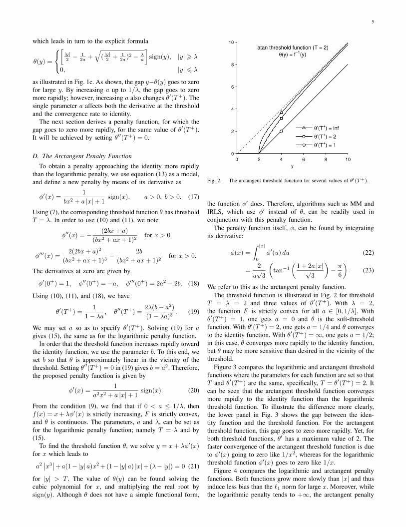
Fig. 2. The arctangent threshold function for several values of θ′(T+).

the function φ′ does. Therefore, algorithms such as MM andIRLS, which use φ′ instead of θ, can be readily used inconjunction with this penalty function.

The penalty function itself, φ, can be found by integratingits derivative:

φ(x) =

∫ |x|

0

φ′(u) du (22)

=2

a√3

(tan−1

(1 + 2a |x|√

3

)− π

6

). (23)

We refer to this as the arctangent penalty function.The threshold function is illustrated in Fig. 2 for threshold

T = λ = 2 and three values of θ′(T+). With λ = 2,the function F is strictly convex for all a ∈ [0, 1/λ]. Withθ′(T+) = 1, one gets a = 0 and θ is the soft-thresholdfunction. With θ′(T+) = 2, one gets a = 1/4 and θ convergesto the identity function. With θ′(T+) =∞, one gets a = 1/2;in this case, θ converges more rapidly to the identity function,but θ may be more sensitive than desired in the vicinity of thethreshold.

Figure 3 compares the logarithmic and arctangent thresholdfunctions where the parameters for each function are set so thatT and θ′(T+) are the same, specifically, T = θ′(T+) = 2. Itcan be seen that the arctangent threshold function convergesmore rapidly to the identity function than the logarithmicthreshold function. To illustrate the difference more clearly,the lower panel in Fig. 3 shows the gap between the iden-tity function and the threshold function. For the arctangentthreshold function, this gap goes to zero more rapidly. Yet, forboth threshold functions, θ′ has a maximum value of 2. Thefaster convergence of the arctangent threshold function is dueto φ′(x) going to zero like 1/x2, whereas for the logarithmicthreshold function φ′(x) goes to zero like 1/x.

Figure 4 compares the logarithmic and arctangent penaltyfunctions. Both functions grow more slowly than |x| and thusinduce less bias than the `1 norm for large x. Moreover, whilethe logarithmic penalty tends to +∞, the arctangent penalty

6 IEEE TRANSACTIONS ON SIGNAL PROCESSING. 2014 (PREPRINT)6

0 2 4 6 8 100

2

4

6

8

10

y

Threshold functions

!’(T+) = 2

atan

log

0 5 10 15 20 25 300

0.5

1

1.5

2

2.5

y

y ! !(y)

log

atan

Fig. 3. Comparison of arctangent and logarithmic penalty functions, bothwith ✓0(T+) = 2. The arctangent threshold function approaches the identityfaster than the logarithmic penalty function.

!30 !20 !10 0 10 20 300

10

20

30

x

Penalty functions, !(x)

|x|log

atan

Fig. 4. Sparsity promoting penalties: absolute value (`1 norm), logarithmic,and arctangent penalty functions (a = 0.25).

faster convergence of the arctangent threshold function is dueto �0(x) going to zero like 1/x2, whereas for the logarithmicthreshold function �0(x) goes to zero like 1/x.

Figure 4 compares the logarithmic and arctangent penaltyfunctions. Both functions grow more slowly than |x| and thusinduce less bias than the `1 norm for large x. Moreover, whilethe logarithmic penalty tends to +1, the arctangent penaltytends to a constant. Hence, the arctangent penalty leads to lessbias than the logarithmic penalty. All three penalties have the

same slope (of 1) at x = 0; and furthermore, the logarithmicand arctangent penalties have the same second derivative (of�a) at x = 0. But, the logarithmic and arctangent penaltieshave different third-order derivatives at x = 0 (2a2 and zero,respectively). That is, the arctangent penalty is more concaveat the origin than the logarithmic penalty.

E. Other Penalty Functions

The firm threshold function [30], and the smoothly clippedabsolute deviation (SCAD) threshold function [23], [71] alsoprovide a compromise between hard and soft thresholding.Both the firm and SCAD threshold functions are continuousand equal to the identity function for large |y| (the corre-sponding �0(x) is equal to zero for x above some value).Some algorithms, such as IRLS, MM, etc., involve dividingby �0, and for these algorithms, divide-by-zero issues arise.Hence, the penalty functions corresponding to these thresholdfunctions are unsuitable for these algorithms.

A widely used penalty function is the `p pseudo-norm, 0 <p < 1, for which �(x) = |x|p . However, using (9), it canbe seen that for this penalty function, the cost function F (x)is not convex for any 0 < p < 1. As our current interest isin non-convex penalty functions for which F is convex, wedo not further discuss the `p penalty. The reader is referredto [42], [51] for in-depth analysis of this and several otherpenalty functions.

F. Denoising Example

To illustrate the trade-off between ✓0(T+) and the biasintroduced by thresholding, we consider the denoising of thenoisy signal illustrated in Fig. 5. Wavelet domain thresholdingis performed with several thresholding functions.

Each threshold function is applied with the same threshold,T = 3�. Most of the noise (c.f. the ‘three-sigma rule’) willfall below the threshold and will be eliminated. The RMSE-optimal choice of threshold is usually lower than 3�, so thisrepresents a larger threshold than that usually used. However,a larger threshold reduces the number of spurious noise peaksproduced by hard thresholding.

The hard threshold achieves the best RMSE, but the outputsignal exhibits spurious noise bursts due to noisy wavelet co-efficients exceeding the threshold. The soft threshold functionreduces the spurious noise bursts, but attenuates the peaks andresults in a higher RMSE. The arctangent threshold functionsuppresses the noise bursts, with modest attenuation of peaks,and results in an RMSE closer to that of hard thresholding.

In this example, the signal is ‘bumps’ from WaveLab[19], with length 2048. The noise is additive white Gaussiannoise with standard deviation � = 0.4. The wavelet is theorthonormal Daubechies wavelet with 3 vanishing moments.

III. SPARSITY PENALIZED LEAST SQUARES

Consider the linear model,

y = Hx + w (24)

where x 2 RN is a sparse N -point signal, y 2 RM isthe observed signal, H 2 RM⇥N is a linear operator (e.g.,

Fig. 3. Comparison of arctangent and logarithmic penalty functions, bothwith θ′(T+) = 2. The arctangent threshold function approaches the identityfaster than the logarithmic penalty function.

−30 −20 −10 0 10 20 30

0

10

20

30

x

Penalty functions, φ(x)

|x|

log

atan

Fig. 4. Sparsity promoting penalties: absolute value (`1 norm), logarithmic,and arctangent penalty functions (a = 0.25).

tends to a constant. Hence, the arctangent penalty leads to lessbias than the logarithmic penalty. All three penalties have thesame slope (of 1) at x = 0; and furthermore, the logarithmicand arctangent penalties have the same second derivative (of−a) at x = 0. But, the logarithmic and arctangent penaltieshave different third-order derivatives at x = 0 (2a2 and zero,respectively). That is, the arctangent penalty is more concaveat the origin than the logarithmic penalty.

E. Other Penalty Functions

The firm threshold function [32], and the smoothly clippedabsolute deviation (SCAD) threshold function [24], [73] alsoprovide a compromise between hard and soft thresholding.Both the firm and SCAD threshold functions are continuousand equal to the identity function for large |y| (the corre-sponding φ′(x) is equal to zero for x above some value).Some algorithms, such as IRLS, MM, etc., involve dividingby φ′, and for these algorithms, divide-by-zero issues arise.Hence, the penalty functions corresponding to these thresholdfunctions are unsuitable for these algorithms.

A widely used penalty function is the `p pseudo-norm, 0 <p < 1, for which φ(x) = |x|p . However, using (9), it canbe seen that for this penalty function, the cost function F (x)is not convex for any 0 < p < 1. As our current interest isin non-convex penalty functions for which F is convex, wedo not further discuss the `p penalty. The reader is referredto [44], [53] for in-depth analysis of this and several otherpenalty functions.

F. Denoising Example

To illustrate the trade-off between θ′(T+) and the biasintroduced by thresholding, we consider the denoising of thenoisy signal illustrated in Fig. 5. Wavelet domain thresholdingis performed with several thresholding functions.

Each threshold function is applied with the same threshold,T = 3σ. Most of the noise (c.f. the ‘three-sigma rule’) willfall below the threshold and will be eliminated. The RMSE-optimal choice of threshold is usually lower than 3σ, so thisrepresents a larger threshold than that usually used. However,a larger threshold reduces the number of spurious noise peaksproduced by hard thresholding.

The hard threshold achieves the best RMSE, but the outputsignal exhibits spurious noise bursts due to noisy wavelet co-efficients exceeding the threshold. The soft threshold functionreduces the spurious noise bursts, but attenuates the peaks andresults in a higher RMSE. The arctangent threshold functionsuppresses the noise bursts, with modest attenuation of peaks,and results in an RMSE closer to that of hard thresholding.

In this example, the signal is ‘bumps’ from WaveLab[20], with length 2048. The noise is additive white Gaussiannoise with standard deviation σ = 0.4. The wavelet is theorthonormal Daubechies wavelet with 3 vanishing moments.

III. SPARSITY PENALIZED LEAST SQUARES

Consider the linear model,

y = Hx+w (24)

where x ∈ RN is a sparse N -point signal, y ∈ RM isthe observed signal, H ∈ RM×N is a linear operator (e.g.,convolution), and w ∈ RN is additive white Gaussian noise(AWGN). The vector x is denoted x = (x0, . . . , xN−1)T .

Under the assumption that x is sparse, we consider the linearinverse problem:

arg minx∈RN

{F (x) =

1

2‖y−Hx‖22 +

N−1∑

n=0

λnφ(xn; an)

}(25)

7

0 500 1000 1500 2000

0

2

4Data

0 500 1000 1500 2000

0

2

4Hard threshold function. RMSE = 0.157

0 500 1000 1500 2000

0

2

4Soft threshold function. RMSE = 0.247

0 500 1000 1500 2000

0

2

4Arctangent threshold function. RMSE = 0.179

Fig. 5. Denoising via orthonormal wavelet thresholding using variousthreshold functions.

where φ(x; a) is a sparsity-promoting penalty function withparameter a, such as the logarithmic or arctangent penaltyfunctions. In many applications, all λn are equal, i.e., λn = λ.For generality, we let this regularization parameter depend onthe index n.

In the following, we address the question of how to con-strain the regularization parameters λn and an so as to ensureF is convex, even when φ( · ; an) is not convex. A problemof this form is addressed in GNC [6], [50], where the an areconstrained to be equal.

A. Convexity Condition

Let φ(x; a) denote a penalty function with parameter a.Consider the function v : R→ R, defined as

v(x) =1

2x2 + λφ(x; a). (26)

Assume v(x) can be made strictly convex for special choicesof λ and a. We give a name to the set of all such choices.

Definition 1. Let S be the set of pairs (λ, a) for which v(x)in (26) is strictly convex. We refer to S as the ‘parameter setassociated with φ’.

For the logarithmic and arctangent penalty functions de-scribed above, the set S is given by

S = {(λ, a) : λ > 0, 0 6 a 6 1/λ}. (27)

Now, consider the function F : RN → R, defined in (25).The following proposition provides a sufficient condition on(λn, an) ensuring the strict convexity of F .

Proposition 2. Suppose R is a positive definite diagonal ma-trix such that HTH−R is positive semidefinite. Let rn denotethe n-th diagonal entry of R, i.e., [R]n,n = rn > 0. Also, letS be the parameter set associated with φ. If (λn/rn, an) ∈ Sfor each n, then F (x) in (25) is strictly convex.

Proof: The function F (x) can be written as

F (x) =1

2xT (HTH−R)x− yTHx+

1

2yTy

︸ ︷︷ ︸q(x)

+g(x), (28)

whereg(x) =

1

2xTRx+

∑

n

λnφ(xn; an). (29)

Note that q(x) is convex since HTH−R is positive semidef-inite. Now, since R is diagonal, we can rewrite g(x) as

g(x) =∑

n

rn2x2n + λnφ(xn; an) (30)

=∑

n

rn

(12x2n +

λnrnφ(xn; an)

). (31)

From (31), it follows that if (λn/rn, an) ∈ S for each n, theng(x) is strictly convex. Under this condition, being a sum ofa convex and a strictly convex function, it follows that F (x)is strictly convex.

The proposition states that constraints on the penalty pa-rameters an ensuring strict convexity of F (x) can be obtainedusing a diagonal matrix R lower bounding HTH. If H doesnot have full rank, then strict convexity is precluded. In thatcase, HTH will be positive semidefinite. Consequently, R willalso be positive semidefinite, with some rn equal to zero. Forthose indices n, where rn = 0, the quadratic term in (30)vanishes. In that case, we can still ensure the convexity of Fin (25) by ensuring φ(x; an) is convex. For the logarithmicand arctangent penalties proposed in this paper, we haveφ(x; a) → |x| as a → 0. Therefore, we define φ(x; 0) = |x|for the log and atan penalties.

In view of (27), the following is a corollary of this result.

Corollary 1. For the logarithmic and arctangent penaltyfunctions, if

0 < an <rnλn, (32)

then F in (25) is strictly convex.

We illustrate condition (32) with a simple example usingN = 2 variables. We set H = I, y = [9.5, 9.5]T , andλ0 = λ1 = 10. Then R = I is a positive diagonal matrixwith HTH − R positive semidefinite. According to (32), Fis strictly convex if ai < 0.1, i = 0, 1. Figure 6 illustratesthe contours of the logarithmic penalty function and the cost

8 IEEE TRANSACTIONS ON SIGNAL PROCESSING. 2014 (PREPRINT)

||x||1, a = 0.0

x0

x1

−6 −3 0 3 6−6

−3

0

3

6

||y − Hx||2

2 + λ ||x||

1

x0x1

0 2 4 60

2

4

6

φ(x, a), a = 0.1

x0

x1

−6 −3 0 3 6−6

−3

0

3

6

||y − Hx||2

2 + λ φ(x, a), a = 0.1

x0

x1

0 2 4 60

2

4

6

φ(x, a), a = 0.2

x0

x1

−6 −3 0 3 6−6

−3

0

3

6

||y − Hx||2

2 + λ φ(x, a), a = 0.2

x0

x1

0 2 4 60

2

4

6

Fig. 6. Contour plots of the logarithmic penalty function φ and cost functionF for three values of a as described in the text. For a = 0.1, the function Fis convex even though the penalty function is not.

function F for three values of a. For a = 0, the penaltyfunction reduces to the `1 norm. Both the penalty function andF are convex. For a = 0.1, the penalty function is non-convexbut F is convex. The non-convexity of the penalty is apparentin the figure (its contours do not enclose convex regions).The non-convex ‘star’ shaped contours induce sparsity morestrongly than the diamond shaped contours of the `1 norm. Fora = 0.2, both the penalty function and F are non-convex. Thenon-convexity of F is apparent in the figure (a convex functioncan not have more than one stationary point, while the figureshows two). In this case, the star shape is too pronounced forF to be convex. In this example, a = 0.1 yields the maximallysparse convex (MSC) problem.

Can a suitable R be obtained by variational principles? Letus denote the minimal eigenvalue of HTH by αmin. ThenR = αminI is a positive semidefinite diagonal lower bound, asneeded. However, this is a sub-optimal lower bound in general.For example, if H is a non-constant diagonal matrix, then atighter lower bound is HTH itself, which is very differentfrom αminI. A tighter lower bound is of interest because the

tighter the bound, the more non-convex the penalty functioncan be, while maintaining convexity of F . In turn, sparsersolutions can be obtained without sacrificing convexity ofthe cost function. A tighter lower bound can be found asthe solution to an optimization problem, as described in thefollowing.

B. Diagonal Lower Bound Matrix ComputationGiven H, the convexity conditions above calls for a positive

semidefinite diagonal matrix R lower bounding HTH. Inorder to find a reasonably tight lower bound, each rn shouldbe maximized. However, these N parameters must be chosenjointly to ensure HTH − R is positive semidefinite. Weformulate the calculation of R as an optimization problem:

arg maxr∈RN

N−1∑

n=0

rn

such that rn > αmin

HTH−R > 0

(33)

where R is the diagonal matrix [R]n,n = rn. The inequalityHTH − R > 0 expresses the constraint that HTH − R ispositive semidefinite (all its eigenvalues non-negative). Notethat the problem is feasible, because R = αminI satisfiesthe constraints. We remark that problem (33) is not the onlyapproach to derive a matrix R satisfying Proposition 2. Forexample, the objective function could be a weighted sum orother norm of {rn}. One convenient aspect of (33) is that ithas the form of a standard convex problem.

Problem (33) can be recognized as a semidefinite optimiza-tion problem, a type of convex optimization problem for whichalgorithms have been developed and for which software isavailable [2]. The cost function in (33) is a linear functionof the N variables, and the constraints are linear matrixinequalities (LMIs). To solve (33) and obtain R, we have usedthe MATLAB software package ‘SeDuMi’ [64].

Often, inverse problems arising in signal processing involvelarge data sets (e.g., speech, EEG, and images). Practical algo-rithms must be efficient in terms of memory and computation.In particular, they should be ‘matrix-free’, i.e., the operatorH is not explicitly stored as a matrix, nor are individualrows or columns of H accessed or modified. However, op-timization algorithms for semidefinite programming usuallyinvolve row/column matrix operations and are not ‘matrixfree’. Hence, solving problem (33) will likely be a bottleneckfor large scale problems. (In the deconvolution example below,the MSC solution using SDP takes from 35 to 55 times longerto compute than the `1 norm solution). This motivates thedevelopment of semidefinite algorithms to solve (33) whereH is not explicitly available, but for which multiplications byH and HT are fast (this is not addressed in this paper).

Nevertheless, for 1D problems of ‘medium’-size (arisingfor example in biomedical applications [61]), (33) is readilysolved via existing software. In case (33) is too computation-ally demanding, then the suboptimal choice R = αminI canbe used as in GNC [6], [50]. Furthermore, we describe belowa multistage algorithm whereby the proposed MSC approachis applied iteratively.

9

C. Optimality Conditions and Threshold Selection

When the cost function F in (25) is strictly convex, thenits minimizer must satisfy specific conditions [29], [4, Prop1.3]. These conditions can be used to verify the optimality ofa solution produced by a numerical algorithm. The conditionsalso aid in setting the regularization parameters λn.

If F in (25) is strictly convex, and φ is differentiable exceptat zero, then x∗ minimizes F if

1

λn[HT (y −Hx∗)]n = φ′(x∗n; an), x∗n 6= 0

1

λn[HT (y −Hx∗)]n ∈ [φ′(0−; an), φ

′(0+; an)], x∗n = 0

(34)where [v]n denotes the n-th component of the vector v.

The optimality of a numerically obtained solution can beillustrated by a scatter plot of [HT (y − Hx)]n/λn versusxnan, for n ∈ ZN . For the example below, Fig. 8 illustratesthe scatter plot, wherein the points lie on the graph of φ′. Weremark that the scatter plot representation as in Fig. 8 makessense only when the parametric penalty φ(x; a) is a functionof ax and a, as are the log and atan penalties, (12) and (23).Otherwise, the horizontal axis will not be labelled xnan andthe points will not lie on the graph of φ. This might not bethe case for other parametric penalties.

The condition (34) can be used to set the regularizationparameters, λn, as in Ref. [30]. Suppose y follows the model(24) where x is sparse. One approach for setting λn is to askthat the solution to (25) be all-zero when x is all-zero in themodel (24). Note that, if x = 0, then y consists of noise only(i.e., y = w). In this case, (34) suggests that λn be chosensuch that

λn φ′(0−; an) 6 [HTw]n 6 λn φ′(0+; an), n ∈ ZN . (35)

For the `1 norm, logarithmic and arctangent penalty functions,φ(0−; an) = −1 and φ(0+; an) = 1, so (35) can be writtenas ∣∣[HTw]n

∣∣ 6 λn, n ∈ ZN . (36)

However, the larger λn is, the more xn will be attenuated.Hence, it is reasonable to set λn to the smallest value satisfying(36), namely,

λn ≈ max∣∣[HTw]n

∣∣ (37)

where w is the additive noise. Although (37) assumes avail-ability of the noise signal w, which is unknown in practice,(37) can often be estimated based on knowledge of statisticsof the noise w. For example, based on the ‘three-sigma rule’,we obtain

λn ≈ 3 std([HTw]n). (38)

If w is white Gaussian noise with variance σ2, then

std([HTw]n) = σ‖H(·, n)‖2 (39)

where H(·, n) denotes column n of H. For example, if Hdenotes linear convolution, then all columns of H have equalnorm and (38) becomes

λn = λ ≈ 3σ‖h‖2 (40)

where h is the impulse of the convolution system.

D. Usage of Method

We summarize the forgoing approach, MSC, to sparsitypenalized least squares, cf. (25). We assume the parametersλn are fixed (e.g., set according to additive noise variance).

1) Input: y ∈ RM , H ∈ RM×N , {λn > 0, n ∈ ZN},φ : R× R→ R.

2) Find a positive semidefinite diagonal matrix R such thatHTH − R is positive semidefinite; i.e., solve (33), oruse the sub-optimal R = αminI. Denote the diagonalelements of R by rn, n ∈ ZN .

3) For n ∈ ZN , set an such that (rn/λn, an) ∈ S . Here,S is the set such that v in (26) is convex if (λ, a) ∈ S.

4) Minimize (25) to obtain x.5) Output: x ∈ RN . �The penalty function φ need not be the logarithmic or arct-

angent penalty functions discussed above. Another parametricpenalty function can be used, but it must have the propertythat v in (26) is convex for (λ, a) ∈ S for some set S. Notethat φ(x, p) = |x|p with 0 < p < 1 does not qualify becausev is non-convex for all 0 < p < 1. On the other hand, the firmpenalty function [32] could be used.

In step (3), for the logarithmic and arctangent penaltyfunctions, one can use

an = βrnλn, where 0 6 β 6 1. (41)

When β = 0, the penalty function is simply the `1 norm; inthis case, the proposed method offers no advantage relativeto `1 norm penalized least squares (BPD/lasso). When β =1, the penalty function is maximally non-convex (maximallysparsity-inducing) subject to F being convex. Hence, as it isnot an arbitrary choice, β = 1 can be taken as a recommendeddefault value. We have used β = 1 in the examples below.

The minimization of (25) in step (4) is a convex opti-mization problem for which numerous algorithms have beendeveloped as noted in Sec. I-B. The most efficient algorithmdepends primarily on the properties of H.

E. Iterative MSC (IMSC)

An apparent limitation of the proposed approach, MSC, isthat for some problems of interest, the parameters rn are eitherequal to zero or nearly equal to zero for all n ∈ ZN , i.e.,R ≈ 0. In this case, the method requires that φ(· ; an) beconvex or practically convex. For example, for the logarithmicand arctangent penalty functions, rn ≈ 0 leads to an ≈ 0. As aconsequence, the penalty function is practically the `1 norm.In this case, the method offers no advantage in comparisonwith `1 norm penalized least squares (BPD/lasso).

The situation wherein R ≈ 0 arises in two standardsparse signal processing problems: basis pursuit denoisingand deconvolution. In deconvolution, if the system is non-invertible or nearly singular (i.e., the frequency response hasa null or approximate null at one or more frequencies), thenthe lower bound R will be R ≈ 0. In BPD, the matrixH often represents the inverse of an overcomplete frame (ordictionary), in which case the lower bound R is again closeto zero.

10 IEEE TRANSACTIONS ON SIGNAL PROCESSING. 2014 (PREPRINT)

In order to broaden the applicability of MSC, we describeiterative MSC (IMSC) wherein MSC is applied several times.On each iteration, MSC is applied only to the non-zeroelements of the sparse solution x obtained as a result of theprevious iteration. Each iteration involves only those columnsof H corresponding to the previously identified non-zero com-ponents. As the number of active columns of H diminishes asthe iterations progress, the problem (33) produces a sequenceof increasingly positive diagonal matrices R. Hence, as theiterations progress, the penalty functions become increasinglynon-convex. The procedure can be repeated until there is nochange in the index set of non-zero elements.

The IMSC algorithm can be initialized with the `1 normsolution, i.e., using φ(x, an) = |x| for all n ∈ ZN . (For thelogarithmic and arctangent penalties, an = 0, n ∈ ZN .) Weassume the `1 norm solution is reasonably sparse; otherwise,sparsity is likely not useful for the problem at hand. Thealgorithm should be terminated when there is no change (oronly insignificant change) between the active set from oneiteration to the next.

The IMSC procedure is described as follows, where i > 1denotes the iteration index.

1) Initialization. Find the `1 norm solution:

x(1) = arg minx∈RN

‖y −Hx‖22 +N−1∑

n=0

λn |xn| . (42)

Set i = 1 and K(0) = N . Note H is of size M ×N .2) Identify the non-zero elements of x(i), and record their

indices in the set K(i),

K(i) ={n ∈ ZN

∣∣∣ x(i)n 6= 0}. (43)

This is the support of x(i). Let K(i) be the number ofnon-zero elements of x(i), i.e., K(i) =

∣∣K(i)∣∣.

3) Check the termination condition: If K(i) is not less thanK(i−1), then terminate. The output is x(i).

4) Define H(i) as the sub-matrix of H containing onlycolumns k ∈ K(i). The matrix H(i) is of size M×K(i).Find a positive semidefinite diagonal matrix R(i) lowerbounding [H(i)]TH(i), i.e., solve problem (33) or useα(i)minI. The matrix R(i) is of size K(i) ×K(i).

5) Set an such that (λn/r(i)n , an) ∈ S, n ∈ K(i). For

example, with the logarithmic and arctangent penalties,one may set

a(i)n = βr(i)n

λn, n ∈ K(i) (44)

for some 0 6 β 6 1.6) Solve the K(i) dimensional convex problem:

u(i) = arg minu∈RK(i)

‖y−H(i)u‖22+∑

n∈K(i)

λnφ(un; a(i)n ).

(45)7) Set x(i+1) as

x(i+1)n =

{0, n /∈ K(i)

u(i)n , n ∈ K(i).

(46)

8) Set i = i+ 1 and go to step 2). �

In the IMSC algorithm, the support of x(i) can only shrinkfrom one iteration to the next, i.e., K(i+1) ⊆ K(i) andK(i+1) 6 K(i). Once there is no further change in K(i), eachsubsequent iteration will produce exactly the same result, i.e.,

K(i+1) = K(i) =⇒ x(i+1) = x(i). (47)

For this reason, the procedure should be terminated whenK(i) ceases to shrink. In the 1D sparse deconvolution examplebelow, the IMSC procedure terminates after only three or fouriterations.

Note that the problem (33) in step 4) reduces in size as thealgorithm progresses. Hence each instance of (33) requires lesscomputation than the previous. More importantly, each matrixH(i+1) has a subset of the columns of H(i). Hence, R(i+1) isless constrained than R(i), and the penalty functions becomemore non-convex (more strongly sparsity-inducing) as theiterations progress. Therefore, the IMSC algorithm producesa sequence of successively sparser x(i).

Initializing the IMSC procedure with the `1 norm solutionsubstantially reduces the computational cost of the algorithm.Note that if the `1 norm solution is sparse, i.e., K(1) � N ,then all the semidefinite optimization problems (33) have farfewer variables than N , i.e., K(i) 6 K(1). Hence, IMSCcan be applied to larger data sets than would otherwise becomputationally practical, due to the computational cost of(33).

F. Deconvolution Example

A sparse signal x(n) of length N = 1000 is generated sothat (i) the inter-spike interval is uniform random between 5and 35 samples, and (ii) the amplitude of each spike is uniformbetween −1 and 1. The signal is illustrated in Fig. 7.

The spike signal is then used as the input to a linear time-invariant (LTI) system, the output of which is contaminatedby AWGN, w(n). The observed data, y(n), is written as

y(n) =∑

k

b(k)x(n− k)−∑

k

a(k) y(n− k) + w(n)

where w(n) ∼ N (0, σ2). It can also be written as

y = A−1Bx+w = Hx+w, H = A−1B

where A and B are banded Toeplitz matrices [60]. In thisexample, we set b(0) = 1, b(1) = 0.8, a(0) = 1, a(1) =−1.047, a(2) = 0.81, and σ = 0.2. The observed data, y, isillustrated in Fig. 7.

Several algorithms for estimating the sparse signal x willbe compared. The estimated signal is denoted x. The accuracyof the estimation is quantified by the `2 and `1 norms of theerror signal and by the support error, denoted L2E, L1E, andSE respectively.

1) L2E = ‖x− x‖22) L1E = ‖x− x‖13) SE = ‖s(x)− s(x)‖0

11

0 200 400 600 800 1000

−1

0

1Spike signal

0 200 400 600 800 1000

−2

0

2 Observed data (simulated)

0 200 400 600 800 1000

−1

0

1Sparse deconvolution (L1 norm)

L2E = 1.439, L1E = 9.40, SE = 30 λ = 2.01

0 200 400 600 800 1000

−1

0

1Sparse deconvolution (L1 + debiasing)

L2E = 0.853, L1E = 5.63, SE = 30 λ = 2.01

0 200 400 600 800 1000

−1

0

1Sparse deconvolution (IMSC (atan))

L2E = 0.705, L1E = 3.97, SE = 13 λ = 2.01

Fig. 7. Sparse deconvolution via sparsity penalized least squares.

The support error, SE, is computed using s(x), the ε-supportof x ∈ RN . Namely, s : RN → {0, 1}N is defined as

[s(x)]n =

{1, |xn| > ε

0, |xn| 6 ε(48)

where ε > 0 is a small value to accommodate negligible non-zeros. We set ε = 10−3. The support error, SE, counts both thefalse zeros and the false non-zeros of x. The numbers of falsezeros and false non-zeros are denoted FZ and FN, respectively.

First, the sparse `1 norm solutions, i.e., φ(x, a) = |x| in(25), with and without debiasing, are computed.1 We set λnaccording to (40), i.e., λn = 2.01, n ∈ ZN . The estimatedsignals are illustrated in Fig. 7. The errors L2E, L1E, and SE,are noted in the figure. As expected, debiasing substantiallyimproves the L2E and L1E errors of the `1 norm solution;

1Debiasing is a post-processing step wherein least squares is performedover the obtained support set [27].

TABLE ISPARSE DECONVOLUTION EXAMPLE. AVERAGE ERRORS (200 TRIALS).

Algorithm L2E L1E SE ( FZ, FN)

`1 norm 1.443 10.01 37.60 (10.3, 27.3)`1 norm + debiasing 0.989 7.14 37.57 (10.3, 27.2)AIHT [7] 1.073 6.37 24.90 (12.4, 12.5)ISD [68] 0.911 5.19 19.67 (11.6, 8.1)SBR [63] 0.788 4.05 13.62 (12.0, 1.6)`p(p = 0.7) IRL2 0.993 5.80 16.32 (12.9, 3.4)`p(p = 0.7) IRL2 + debiasing 0.924 4.82 16.32 (12.9, 3.4)`p(p = 0.7) IRL1 0.884 5.29 14.43 (11.5, 2.9)`p(p = 0.7) IRL1 + debiasing 0.774 4.18 14.43 (11.5, 2.9)IMSC (log) 0.864 5.08 17.98 ( 9.8, 8.2)IMSC (log) + debiasing 0.817 4.83 17.98 ( 9.8, 8.2)IMSC (atan) 0.768 4.29 15.43 (10.0, 5.5)IMSC (atan) + debiasing 0.769 4.35 15.42 (10.0, 5.5)IMSC/S (atan) 0.910 5.45 17.93 ( 9.8, 8.1)IMSC/S (atan) + debiasing 0.800 4.73 17.92 ( 9.8, 8.1)

however, it does not improve the support error, SE. Debiasingdoes not make the solution more sparse. The errors, averagedover 200 trials, are shown in Table I. Each trial consists ofindependently generated sparse and noise signals.

Next, sparse deconvolution is performed using three algo-rithms developed to solve the highly non-convex `0 quasi-norm problem, namely the Iterative Support Detection (ISD)algorithm [68],2 the Accelerated Iterative Hard Thresholding(AIHT) algorithm [7],3 and the Single Best Replacement(SBR) algorithm [63]. In each case, we used software bythe respective authors. The ISD and SBR algorithms requireregularization parameters ρ and λ respectively; we found thatρ = 1.0 and λ = 0.5 were approximately optimal. The AIHTalgorithm requires the number of non-zeros be specified; weused the number of non-zeros in the true sparse signal. Eachof ISD, AIHT, and SBR significantly improve the accuracy ofthe result in comparison with the `1 norm solutions, with SBRbeing the most accurate. These algorithms essentially seek thecorrect support. They do not penalize the values in the detectedsupport; so, debiasing does not alter the signals produced bythese algorithms.

The `p quasi-norm, with p = 0.7, i.e. φ(x) = |x|p,also substantially improves upon the `1 norm result. Severalmethods exist to minimize the cost function F in this case. Weimplement two methods: IRL2 and IRL1 (iterative reweighted`2 and `1 norm minimization, respectively), with and withoutdebiasing in each case. We used λ = 1.0, which we found tobe about optimal on average for this deconvolution problem.As revealed in Table I, IRL1 is more accurate than IRL2.Note that IRL2 and IRL1 seek to minimize exactly the samecost function; so the inferiority of IRL2 compared to IRL1 isdue to the convergence of IRL2 to a local minimizer of F .Also note that debiasing substantially improves L2E and L1E(with no effect on SE) for both IRL2 and IRL1. The `p resultsdemonstrate both the value of a non-convex regularizer and thevulnerability of non-convex optimization to local minimizers.

The results of the proposed iterative MSC (IMSC) algo-rithm, with and without debiasing, are shown in Table I. We

2http://www.caam.rice.edu/%7Eoptimization/L1/ISD/3http://users.fmrib.ox.ac.uk/%7Etblumens/sparsify/sparsify.html

12 IEEE TRANSACTIONS ON SIGNAL PROCESSING. 2014 (PREPRINT)12

cost function; so the inferiority of IRL2 compared to IRL1 isdue to the convergence of IRL2 to a local minimizer of F .Also note that debiasing substantially improves L2E and L1E(with no effect on SE) for both IRL2 and IRL1. The `p resultsdemonstrate both the value of a non-convex regularizer and thevulnerability of non-convex optimization to local minimizers.

The results of the proposed iterative MSC (IMSC) algo-rithm, with and without debiasing, are shown in Table I. Weused � = 1.0 and �n = 2.01, n 2 ZN , in accordance with(40). Results using the logarithmic (log) and arctangent (atan)penalty functions are tabulated, which show the improvementprovided by the later penalty, in terms of L2E, L1E, and SE.While debiasing reduces the error (bias) of the logarithmicpenalty, it has negligible effect on the arctangent penalty. Thesimplified form of the MSC algorithm, wherein R = ↵minI isused instead of the R computed via SDP, is also tabulated inTable I, denoted by IMSC/S. IMSC/S is more computationallyefficient than MSC due to the omission of SDP; however, itdoes lead to an increase in the error measures.

The IMSC algorithm ran for three iterations on average.For example, the IMSC solution illustrated in Fig. 7 ran withK(1) = 61, K(2) = 40, and K(3) = 38. Therefore, eventhough the signal is of length 1000, the SDPs that had to besolved are much smaller: of sizes 61, 40, and 38, only.

The optimality of the MSC solution at each stage can beverified using (34). Specifically, a scatter plot of [HT (y �Hx)]n/�n verses xnan, for all n 2 K(i), should show allpoints lying on the graph of @�(x, 1). For the IMSC solutionillustrated in Fig. 7, this optimality scatter plot is illustratedin Fig. 8, which shows that all points lie on the graph ofsign(x)/(1 + |x| + x2), hence verifying the optimality of theobtained solution.

To more clearly compare the relative bias of the `1 normand IMSC (atan) solutions, these two solutions are illustratedtogether in Fig. 8. Only the non-zero elements of each solutionare shown. In this figure, the closer the points lie to theidentity, the more accurate the solution. The figure shows theIMSC solution lies closer to the identity than the `1 normsolution; and the `1 norm solution tends to underestimate thetrue values.

In terms of L2E and L1E, the best IMSC result, i.e., IMSC(atan), is outperformed by SBR and the IRL1 + debiasingalgorithm. In addition, IMSC (atan) yields lower SE than `1minimization, AIHT, and ISD. IMSC does not yield the besterror measures, but it comes reasonably close; even thoughIMSC is based entirely on convex optimization. In terms ofL1E and SE, the SBR performs best for this example. Mostnotably, SBR attains a small number of false non-zeros.

Note that IMSC requires only the parameter � (with 0 6� 6 1) beyond those parameters (namely �n) required for the`1 norm solution.

Fig. 9 illustrates the average errors as functions of the reg-ularization parameter, for ISD, IMSC, and IMSC + debiasing(denoted IMSC+d in the figure). For IMSC, the regularizationparameter is �. For ISD, the regularization parameter is⇢ = �/2. Note that for IMSC, the value of � minimizing L2Eand L1E depends on whether or not debiasing is performed.The value � suggested by (40) (i.e., � = 2) is reasonably

!4 !2 0 2 4

!1

1(1

/!)

[HT(y

!H

x)] n

xn a

n

Optimality scatter plot ! IMSC (atan)(a)

!1 !0.5 0 0.5 1!1

!0.5

0

0.5

1

True

Est

imate

Sparse deconvolution(b)

L1 normIMSC (atan)

Fig. 8. Sparse deconvolution. (a) Illustration of optimality condition (34) forIMSC (atan) solution. (b) Comparison of `1 norm and IMSC solutions.

effective with or without debiasing. The value of � minimizingSE is somewhat higher.

The implementation of the `1, IRL2, IRL1, and IMSCalgorithms for deconvolution each require the solution of(25) with various penalty functions and/or sub-matrices ofH. We have used algorithms, based on majorization of thepenalty function, that exploit banded matrix structures forcomputational efficiency [59], [60].

Finally, we comment on the computation time for IMSC.The IMSC solution with the atan penalty illustrated in Fig. 7took 1.7 seconds and about 94% of the time was spent onsolving SDPs. As noted above, three SDPs were solved (ofsizes 61, 40, and 38). The IMSC solution with the log penaltytook 2.8 seconds, with again, about 94% of the time spenton SDPs. The longer time was due to more iterations ofIMSC (five SDPs instead of three). The `1 norm solution wasobtained in only 52 milliseconds (33 times faster than the MSCsolution).

IV. CONCLUSION

This paper proposes an approach (MSC) to obtain sparse so-lutions to ill-posed linear inverse problems. In order to inducesparsity more strongly than the `1 norm, the MSC approachutilizes non-convex penalty functions. However, the non-convex penalty functions are constrained so that the total cost

Fig. 8. Sparse deconvolution. (a) Illustration of optimality condition (34)for IMSC (atan) solution. (b) Comparison of `1 norm and IMSC solutions.

used β = 1.0 and λn = 2.01, n ∈ ZN , in accordance with(40). Results using the logarithmic (log) and arctangent (atan)penalty functions are tabulated, which show the improvementprovided by the later penalty, in terms of L2E, L1E, and SE.While debiasing reduces the error (bias) of the logarithmicpenalty, it has negligible effect on the arctangent penalty. Thesimplified form of the MSC algorithm, wherein R = αminI isused instead of the R computed via SDP, is also tabulated inTable I, denoted by IMSC/S. IMSC/S is more computationallyefficient than MSC due to the omission of SDP; however, itdoes lead to an increase in the error measures.

The IMSC algorithm ran for three iterations on average.For example, the IMSC solution illustrated in Fig. 7 ran withK(1) = 61, K(2) = 40, and K(3) = 38. Therefore, eventhough the signal is of length 1000, the SDPs that had to besolved are much smaller: of sizes 61, 40, and 38, only.

The optimality of the MSC solution at each stage can beverified using (34). Specifically, a scatter plot of [HT (y −Hx)]n/λn verses xnan, for all n ∈ K(i), should show allpoints lying on the graph of ∂φ(x, 1). For the IMSC solutionillustrated in Fig. 7, this optimality scatter plot is illustratedin Fig. 8, which shows that all points lie on the graph ofsign(x)/(1 + |x|+ x2), hence verifying the optimality of theobtained solution.

To more clearly compare the relative bias of the `1 normand IMSC (atan) solutions, these two solutions are illustrated

together in Fig. 8. Only the non-zero elements of each solutionare shown. In this figure, the closer the points lie to theidentity, the more accurate the solution. The figure shows theIMSC solution lies closer to the identity than the `1 normsolution; and the `1 norm solution tends to underestimate thetrue values.

In terms of L2E and L1E, the best IMSC result, i.e., IMSC(atan), is outperformed by SBR and the IRL1 + debiasingalgorithm. In addition, IMSC (atan) yields lower SE than `1minimization, AIHT, and ISD. IMSC does not yield the besterror measures, but it comes reasonably close; even thoughIMSC is based entirely on convex optimization. In terms ofL1E and SE, the SBR performs best for this example. Mostnotably, SBR attains a small number of false non-zeros.

Note that IMSC requires only the parameter β (with 0 6β 6 1) beyond those parameters (namely λn) required for the`1 norm solution.

Fig. 9 illustrates the average errors as functions of the reg-ularization parameter, for ISD, IMSC, and IMSC + debiasing(denoted IMSC+d in the figure). For IMSC, the regularizationparameter is λ. For ISD, the regularization parameter isρ = λ/2. Note that for IMSC, the value of λ minimizing L2Eand L1E depends on whether or not debiasing is performed.The value λ suggested by (40) (i.e., λ = 2) is reasonablyeffective with or without debiasing. The value of λ minimizingSE is somewhat higher.

The implementation of the `1, IRL2, IRL1, and IMSCalgorithms for deconvolution each require the solution of(25) with various penalty functions and/or sub-matrices ofH. We have used algorithms, based on majorization of thepenalty function, that exploit banded matrix structures forcomputational efficiency [59], [60].

Finally, we comment on the computation time for IMSC.The IMSC solution with the atan penalty illustrated in Fig. 7took 1.7 seconds and about 94% of the time was spent onsolving SDPs. As noted above, three SDPs were solved (ofsizes 61, 40, and 38). The IMSC solution with the log penaltytook 2.8 seconds, with again, about 94% of the time spenton SDPs. The longer time was due to more iterations ofIMSC (five SDPs instead of three). The `1 norm solution wasobtained in only 52 milliseconds (33 times faster than the MSCsolution).

IV. CONCLUSION

This paper proposes an approach (MSC) to obtain sparse so-lutions to ill-posed linear inverse problems. In order to inducesparsity more strongly than the `1 norm, the MSC approachutilizes non-convex penalty functions. However, the non-convex penalty functions are constrained so that the total costfunction is convex. This approach was introduced in [6], andextended in [50]–[52]. A novelty of the proposed approach isthat the maximally non-convex (maximally sparsity-inducing)penalty functions are found by formulating a semidefiniteprogram (SDP). Iterative MSC (IMSC) consists of applyingMSC to the non-zero (active) elements of the sparse solutionproduced by the previous iteration. Each iteration of IMSCinvolves the solution to a convex optimization problem.

13

1 1.5 2 2.5 3 3.5 4

0.7

0.8

0.9

1

1.1

L2 error

ISD

IMSC/S+d

IMSC

IMSC+d

SBR

1 1.5 2 2.5 3 3.5 4

3

4

5

6

7

8

9L1 error

ISD

IMSC/S+d

IMSC

IMSC+d

SBR

1 1.5 2 2.5 3 3.5 4

10

15

20

25

30Support error

λ (IMSC), 2ρ (ISD), 4λ (SBR)

ISD

IMSC/S+d

IMSC

IMSC+d

SBR

Fig. 9. Sparse deconvolution. Errors as functions of regularization param-eters, averaged over 100 realizations. (Note that the support error for IMSCand IMSC+d coincide.)

The MSC method is intended as a convex alternative to`1 norm minimization, which is widely used in sparse signalprocessing where it is often desired that a ‘sparse’ or the‘sparsest’ solution be found to a system of linear equationswith noise. At the same time, some practitioners are concernedwith non-convex optimization issues. One issue is entrapmentof optimization algorithms in local minima. But another issuerelated to non-convex optimization is the sensitivity of thesolution to perturbations in the data. Suppose a non-convexcost function has two minima, one local, one global. Thecost function surface depends on the observed data. As theobserved data vary, the local (non-global) minimum maydecrease in value relative to the global minimum. Hencethe global minimizer of the non-convex cost function is adiscontinuous function of the data, i.e., the solution mayjump around erratically as a function of observed data. Thisphenomena is exhibited, for example, as spurious noise spikesin wavelet hard-thresholding denoising, as illustrated in Fig.5. For these reasons, some may favor convex formulations.The proposed MSC approach simply considers the question:

what is the convex optimization problem that best promotessparsity (from a parameterized set of penalty functions).

Being based entirely on convex optimization, it can not beexpected that MSC produces solutions as sparse as non-convexoptimization methods, such as `p quasi-norm (0 < p < 1)minimization. However, it provides a principled approach forenhanced sparsity relative to the `1 norm. Moreover, althoughit is not explored here, it may be effective to use MSC inconjunction with other techniques. As has been recognizedin the literature, and as illustrated in the sparse deconvolutionexample above, reweighted `1 norm minimization can be moreeffective than reweighted `2 norm minimization (i.e., higherlikelihood of convergence to a global minimizer). Likewise,it will be of interest to explore the use of reweighted MSCor similar methods as a means of more reliable non-convexoptimization. For example, a non-convex MM-type algorithmmay be conceived wherein a specified non-convex penaltyfunction is majorized by a non-convex function constrainedso as to ensure convexity of the total cost function at eachiteration of MM.

To apply the proposed approach to large scale problems(e.g., image and video reconstruction), it is beneficial to solve(33) by some algorithm that does not rely on accessing ormanipulating individual rows or columns of H.

The technique, where a non-convex penalty is chosen so asto lead to a convex problem, has recently been utilized forgroup-sparse signal denoising in [14].

APPENDIX

Suppose F , defined in (2), is strictly convex and φ(x)is differentiable for all x ∈ R except x = 0. Then thesubdifferential ∂F is given by

∂F (x) =

{{x− y + λφ′(x)}, if x 6= 0,

[λφ′(0−), λφ′(0+)]− y, if x = 0.(49)

Since F is strictly convex, its minimizer x∗ satisfies 0 ∈∂F (x∗).

If y ∈ [λφ′(0−), λφ′(0+)], then from (49) we have 0 ∈∂F (0), and in turn x∗ = 0. Assuming φ is symmetric,then φ′(0−) = −φ(0+), and this interval represents thethresholding interval of θ, and the threshold T is given byT = λφ′(0+).

Suppose now that y /∈ [λφ′(0−), λφ′(0+)]. This happens ifeither (i) y > λφ′(0+), or (ii) y < λφ′(0−). In the following,we study case (i). The results extend to (ii) straightforwardly.

First, note that if y > λφ′(0+), then x∗ > 0 and it satisfies

y = x∗ + λφ′(x∗). (50)

Let us define f : R+ → R as

f(x) = x+ λφ′(x). (51)

Note that, for x > 0, f(x) = F ′(x)+y. Since F (x) is strictlyconvex, F ′(x) and f(x) are strictly increasing, hence injectivefor x > 0. For y > λφ′(0+), the threshold function θ can nowbe expressed as

θ(y) = f−1(y). (52)

14 IEEE TRANSACTIONS ON SIGNAL PROCESSING. 2014 (PREPRINT)

Observe that f is continuous and f(0+) = λφ′(0+) = T .In view of (52), this implies that θ(T+) = 0. Thus, θ(y) iscontinuous at the threshold.

For a symmetric φ, it can be shown that F is strictly convexif and only if f is strictly increasing for x > 0. This in turncan be ensured by requiring φ′′(x) > −1/λ, ∀x > 0.

Let us now find the first and second derivatives of θ(y) aty = T+. From (52), f(θ(y)) = y. Differentiating with respectto y gives

f ′(θ(y)) θ′(y) = 1. (53)

Differentiating again with respect to y gives

f ′′(θ(y)) [θ′(y)]2 + f ′(θ(y)) θ′′(y) = 0. (54)

Setting y = T+ in (53) gives

θ′(T+) = 1/f ′(0+). (55)

Setting y = T+ in (54) gives

f ′′(0+) [θ′(T+)]2 + f ′(0+) θ′′(T+) = 0 (56)

orθ′′(T+) = −f ′′(0+)/[f ′(0+)]3. (57)

Using (51), we have

f ′(0+) = 1 + λφ′′(0+) and f ′′(0+) = λφ′′′(0+). (58)

Equations (10) and (11) follow.

ACKNOWLEDGMENT

The authors thank an anonymous reviewer for detailedsuggestions and corrections that improved the manuscript.

REFERENCES

[1] A. Achim, P. Tsakalides, and A. Bezerianos. SAR image denoisingvia Bayesian wavelet shrinkage based on heavy-tailed modeling. IEEETrans. on Geoscience and Remote Sensing, 41(8):1773–1784, August2003.

[2] A. Antoniou and W. S. Lu. Practical Optimization: Algorithms andEngineering Applications. Springer, 2007.

[3] A. M. Atto, D. Pastor, and G. Mercier. Wavelet shrinkage: unificationof basic thresholding functions and thresholds. Signal, Image and VideoProc., 5:11–28, 2011.

[4] F. Bach, R. Jenatton, J. Mairal, and G. Obozinski. Optimizationwith sparsity-inducing penalties. Foundations and Trends in MachineLearning, 4(1):1–106, 2012.

[5] R. G. Baraniuk, E. Candes, M. Elad, and Y. Ma, editors. Special issueon applications of sparse representation and compressive sensing. Proc.IEEE, 98(6), June 2010.

[6] A. Blake and A. Zisserman. Visual Reconstruction. MIT Press, 1987.[7] A. Blumensath. Accelerated iterative hard thresholding. Signal Process-

ing, 92(3):752–756, 2012.[8] T. Blumensath and M. E. Davies. Normalized iterative hard thresholding:

Guaranteed stability and performance. IEEE. J. Sel. Top. SignalProcessing, 4(2):298–309, April 2010.

[9] S. Boyd, N. Parikh, E. Chu, B. Peleato, and J. Eckstein. Distributedoptimization and statistical learning via the alternating direction methodof multipliers. Foundations and Trends in Machine Learning, 3(1):1–122, 2011.

[10] M. S. O’ Brien, A. N. Sinclair, and S. M. Kramer. Recovery of asparse spike time series by L1 norm deconvolution. IEEE Trans. SignalProcess., 42(12):3353–3365, December 1994.

[11] E. J. Candes, M. B. Wakin, and S. Boyd. Enhancing sparsity byreweighted l1 minimization. J. Fourier Anal. Appl., 14(5):877–905,December 2008.

[12] P. Charbonnier, L. Blanc-Feraud, G. Aubert, and M. Barlaud. Determin-istic edge-preserving regularization in computed imaging. IEEE Trans.Image Process., 6(2):298–311, February 1997.

[13] R. Chartrand. Fast algorithms for nonconvex compressive sensing: MRIreconstruction from very few data. In IEEE Int. Symp. Biomed. Imag.(ISBI), pages 262–265, July 2009.

[14] P.-Y. Chen and I. W. Selesnick. Group-sparse signaldenoising: Non-convex regularization, convex optimization.http://arxiv.org/abs/1308.5038, August 2013.

[15] S. Chen, D. L. Donoho, and M. A. Saunders. Atomic decomposition bybasis pursuit. SIAM J. Sci. Comput., 20(1):33–61, 1998.

[16] J. F. Claerbout and F. Muir. Robust modeling of erratic data. Geophysics,38(5):826–844, 1973.

[17] M. Clyde and E. I. George. Empirical Bayes estimation in waveletnonparametric regression. In P. Muller and B. Vidakovic, editors,Bayesian Inference in Wavelet Based Models, pages 309–322. Springer-Verlag, 1999.

[18] P. L. Combettes and J.-C. Pesquet. Proximal thresholding algorithmfor minimization over orthonormal bases. SIAM J. Optim., 18(4):1351–1376, 2008.

[19] P. L. Combettes and J.-C. Pesquet. Proximal splitting methods in signalprocessing. In H. H. Bauschke et al., editors, Fixed-Point Algorithms forInverse Problems in Science and Engineering, pages 185–212. Springer-Verlag, 2011.

[20] D. Donoho, A. Maleki, and M. Shahram. Wavelab 850.http://www-stat.stanford.edu/%7Ewavelab/.

[21] D. L. Donoho and I. M. Johnstone. Ideal spatial adaptation by waveletshrinkage. Biometrika, 81(3):425–455, 1994.

[22] E. Esser, X. Zhang, and T. F. Chan. A general framework for a classof first order primal-dual algorithms for convex optimization in imagingscience. SIAM J. Imag. Sci., 3(4):1015–1046, 2010.

[23] J. M. Fadili and L. Boubchir. Analytical form for a Bayesian waveletestimator of images using the Bessel K form densities. IEEE Trans.Image Process., 14(2):231–240, February 2005.

[24] J. Fan and R. Li. Variable selection via nonconcave penalized likelihoodand its oracle properties. J. Amer. Statist. Assoc., 96(456):1348–1360,2001.

[25] M. Figueiredo, J. Bioucas-Dias, and R. Nowak. Majorization-minimization algorithms for wavelet-based image restoration. IEEETrans. Image Process., 16(12):2980–2991, December 2007.

[26] M. Figueiredo and R. Nowak. Wavelet-based image estimation: Anempirical Bayes approach using Jeffrey’s noninformative prior. IEEETrans. Image Process., 10(9):1322–1331, September 2001.

[27] M. A. T. Figueiredo, R. D. Nowak, and S. J. Wright. Gradient projectionfor sparse reconstruction: Application to compressed sensing and otherinverse problems. IEEE J. Sel. Top. Signal Process., 1(4):586–598,December 2007.

[28] S. Foucart. Hard thresholding pursuit: an algorithm for compressivesensing. SIAM J. Numer. Anal., 49(6):2543–2563, 2010.

[29] J.-J. Fuchs. On sparse representations in arbitrary redundant bases. IEEETrans. Inform. Theory, 50(6):1341–1344, 2004.

[30] J. J. Fuchs. Identification of real sinusoids in noise, the Global MatchedFilter approach. In 15th IFAC Symp. on System Identification, pages1127–1132, Saint-Malo, France, July 2009.

[31] H. Gao. Wavelet shrinkage denoising using the nonnegative garrote. J.Comput. Graph. Statist., 7:469–488, 1998.

[32] H.-Y. Gao and A. G. Bruce. Waveshrink with firm shrinkage. StatisticaSinica, 7:855–874, 1997.

[33] G. Gasso, A. Rakotomamonjy, and S. Canu. Recovering sparse signalswith a certain family of nonconvex penalties and DC programming.IEEE Trans. Signal Process., 57(12):4686–4698, December 2009.

[34] D. Geman and Y. Chengda. Nonlinear image recovery with half-quadratic regularization. IEEE Trans. Image Process., 4(7):932–946,1995.

[35] A. Gholami and S. M. Hosseini. A general framework for sparsity-baseddenoising and inversion. IEEE Trans. Signal Process., 59(11):5202–5211, November 2011.

[36] T. Goldstein and S. Osher. The split Bregman method for L1-regularizedproblems. SIAM J. Imag. Sci., 2(2):323–343, 2009.

[37] I. F. Gorodnitsky and B. D. Rao. Sparse signal reconstruction fromlimited data using FOCUSS: a re-weighted minimum norm algorithm.IEEE Trans. Signal Process., 45(3):600–616, March 1997.

[38] G. Harikumar and Y. Bresler. A new algorithm for computing sparsesolutions to linear inverse problems. In Proc. IEEE Int. Conf. Acoust.,Speech, Signal Processing (ICASSP), volume 3, pages 1331–1334, May1996.

15

[39] A. Hyvarinen. Sparse code shrinkage: Denoising of non-Gaussian databy maximum likelihood estimation. Neural Computation, 11:1739–1768,1999.

[40] S. Ji, Y. Xue, and L. Carin. Bayesian compressive sensing. IEEE Trans.Signal Process., 56(6):2346–2356, June 2008.

[41] K. F. Kaaresen. Deconvolution of sparse spike trains by iterated windowmaximization. IEEE Trans. Signal Process., 45(5):1173–1183, May1997.

[42] N. Kingsbury and T. Reeves. Redundant representation with complexwavelets: how to achieve sparsity. In Proc. IEEE Int. Conf. ImageProcessing, 2003.

[43] I. Kozlov and A. Petukhov. Sparse solutions of underdetermined linearsystems. In W. Freeden et al., editor, Handbook of Geomathematics.Springer, 2010.

[44] D. A. Lorenz. Non-convex variational denoising of images: Interpolationbetween hard and soft wavelet shrinkage. Current Development inTheory and Application of Wavelets, 1(1):31–56, 2007.

[45] S. Mallat. A wavelet tour of signal processing. Academic Press, 1998.[46] H. Mohimani, M. Babaie-Zadeh, and C. Jutten. A fast approach for

overcomplete sparse decomposition based on smoothed l0 norm. IEEETrans. Signal Process., 57(1):289–301, January 2009.

[47] N. Mourad and J. P. Reilly. Minimizing nonconvex functions for sparsevector reconstruction. IEEE Trans. Signal Process., 58(7):3485–3496,July 2010.

[48] S. Nadarajah and S. Kotz. The BKF Bayesian wavelet estimator. SignalProcessing, 87(9):2268–2271, September 2007.

[49] M. Nikolova. Estimation of binary images by minimizing convexcriteria. In Proc. IEEE Int. Conf. Image Processing, pages 108–112vol. 2, 1998.

[50] M. Nikolova. Markovian reconstruction using a GNC approach. IEEETrans. Image Process., 8(9):1204–1220, 1999.

[51] M. Nikolova, J. Idier, and A. Mohammad-Djafari. Inversion of large-support ill-posed linear operators using a piecewise Gaussian MRF.IEEE Trans. Image Process., 7(4):571–585, 1998.

[52] M. Nikolova, M. Ng, S. Zhang, and W. Ching. Efficient reconstructionof piecewise constant images using nonsmooth nonconvex minimization.SIAM J. Imag. Sci., 1(1):2–25, 2008.

[53] M. Nikolova and M. K. Ng. Analysis of half-quadratic minimiza-tion methods for signal and image recovery. SIAM J. Sci. Comput.,27(3):937–966, October 2005.

[54] M. Nikolova, M. K. Ng, and C.-P. Tam. Fast nonconvex nonsmoothminimization methods for image restoration and reconstruction. IEEETrans. Image Process., 19(12):3073–3088, December 2010.

[55] J. Portilla and L. Mancera. L0-based sparse approximation: twoalternative methods and some applications. In Proceedings of SPIE,volume 6701 (Wavelets XII), 2007.

[56] J. Portilla, V. Strela, M. J. Wainwright, and E. P. Simoncelli. Imagedenoising using scale mixtures of Gaussians in the wavelet domain.IEEE Trans. Image Process., 12(11):1338–1351, November 2003.

[57] K. Qiu and A. Dogandzic. Sparse signal reconstruction via ECME hardthresholding. IEEE Trans. Signal Process., 60(9):4551–4569, September2012.

[58] B. D. Rao, K. Engan, S. F. Cotter, J. Palmer, and K. Kreutz-Delgado.Subset selection in noise based on diversity measure minimization. IEEETrans. Signal Process., 51(3):760–770, March 2003.

[59] I. Selesnick. Penalty and shrinkage functions for sparse signal process-ing. Connexions Web site, 2012. http://cnx.org/content/m45134/1.1/.

[60] I. Selesnick. Sparse deconvolution (an MM algorithm). Connexions Website, 2012. http://cnx.org/content/m44991/1.4/.

[61] I. W. Selesnick, S. Arnold, and V. R. Dantham. Polynomial smoothingof time series with additive step discontinuities. IEEE Trans. SignalProcess., 60(12):6305–6318, December 2012.

[62] I. W. Selesnick, H. L. Graber, D. S. Pfeil, and R. L. Barbour. Simultane-ous low-pass filtering and total variation denoising. IEEE Trans. SignalProcess., 2014. To appear.

[63] C. Soussen, J. Idier, D. Brie, and J. Duan. From Bernoulli-Gaussiandeconvolution to sparse signal restoration. IEEE Trans. Signal Process.,59(10):4572–4584, October 2011.

[64] J. F. Sturm. Using SeDuMi 1.02, a MATLAB toolbox foroptimization over symmetric cones. Optimization Methods andSoftware, 11–12:625–653, 1999. Version 1.05 available fromhttp://fewcal.kub.nl/sturm.

[65] X. Tan, W. Roberts, J. Li, and P. Stoica. Sparse learning via iterativeminimization with application to MIMO radar imaging. IEEE Trans.Signal Process., 59(3):1088–1101, March 2011.

[66] H. L. Taylor, S. C. Banks, and J. F. McCoy. Deconvolution with the l1norm. Geophysics, 44(1):39–52, 1979.

[67] R. Tibshirani. Regression shrinkage and selection via the lasso. J. Roy.Statist. Soc., Ser. B, 58(1):267–288, 1996.

[68] Y. Wang and W. Yin. Sparse signal reconstruction via iterative supportdetection. SIAM J. Imag. Sci., 3(3):462–491, 2010.

[69] D. Wipf and S. Nagarajan. Iterative reweighted `1 and `2 methods forfinding sparse solutions. IEEE. J. Sel. Top. Signal Processing, 4(2):317–329, April 2010.

[70] X.-P. Zhang. Thresholding neural network for adaptive noise reduction.IEEE Trans. Neural Networks, 12(3):567–584, May 2001.

[71] X.-P. Zhang and M. D. Desai. Adaptive denoising based on SURE risk.IEEE Signal Processing Letters, 5(10):265–267, October 1998.

[72] Z.-D. Zhao. Wavelet shrinkage denoising by generalized thresholdfunction. In Proc. Int. Conf. Machine Learning and Cybernetics,volume 9, pages 5501–5506, August 2005.

[73] H. Zou and R. Li. One-step sparse estimates in nonconcave penalizedlikelihood models. Ann. Statist., 36(4):1509–1533, 2008.