ICES WKSOUTH REPORT 2014 ICES ADVISORY COMMITTEE ICES CM 2014/ACOM:40 REF. ACOM Report of the Benchmark Workshop on Southern megrim and hake (WKSOUTH) 3-7 February 2014 ICES HQ, Copenhagen, Denmark

Welcome message from author
This document is posted to help you gain knowledge. Please leave a comment to let me know what you think about it! Share it to your friends and learn new things together.
Transcript

ICES WKSOUTH REPORT 2014 ICES ADVISORY COMMITTEE
ICES CM 2014/ACOM:40
REF. ACOM
Report of the Benchmark Workshop on Southern megrim and hake (WKSOUTH)
3-7 February 2014
ICES HQ, Copenhagen, Denmark

International Council for the Exploration of the Sea Conseil International pour l’Exploration de la Mer
H. C. Andersens Boulevard 44–46 DK-1553 Copenhagen V Denmark Telephone (+45) 33 38 67 00 Telefax (+45) 33 93 42 15 www.ices.dk [email protected]
Recommended format for purposes of citation:
ICES. 2014. Report of the Benchmark Workshop on Southern megrim and hake (WKSOUTH), 3-7 February 2014, ICES HQ, Copenhagen, Denmark. ICES CM 2014/ACOM:40. 236 pp.
For permission to reproduce material from this publication, please apply to the Gen-eral Secretary.
The document is a report of an Expert Group under the auspices of the International Council for the Exploration of the Sea and does not necessarily represent the views of the Council.
© 2014 International Council for the Exploration of the Sea

ICES WKSOUTH REPORT 2014 | i
Contents
Executive Summary ............................................................................................................... 3
1 Introduction .................................................................................................................... 5
2 Description of the Benchmark Process ...................................................................... 6
3 Recommendations covering all stocks ....................................................................... 7
4 Hake ................................................................................................................................. 8
4.1 Stock ID and substock structure ......................................................................... 8
4.2 Multispecies and mixed fisheries issues ............................................................ 8 4.3 Ecosystem drivers ................................................................................................. 8
4.4 Northern Hake ...................................................................................................... 8 4.4.1 Issue list ..................................................................................................... 8
4.4.1.1 Model ......................................................................................................... 8
4.4.1.2 Data ............................................................................................................ 8
4.4.2 Scorecard on data quality ....................................................................... 9 4.4.3 Stock Assessment data ............................................................................ 9
4.4.3.1 Catch – quality, misreporting, discards ................................................ 9
4.4.3.2 Surveys .................................................................................................... 12
4.4.3.3 Commercial catch-effort data ............................................................... 13
4.4.3.4 Length, weights, maturities, growth ................................................... 18
4.4.4 Assessment model ................................................................................. 19 4.4.5 Short-term projections ........................................................................... 25 4.4.6 Appropriate Reference Points (MSY) .................................................. 25 4.4.7 Future Research and data requirements ............................................. 32
4.5 Southern Hake..................................................................................................... 33 4.5.1 Issue list ................................................................................................... 33
4.5.1.1 Model ....................................................................................................... 33
4.5.1.2 Data .......................................................................................................... 34
4.5.2 Scorecard on data quality ..................................................................... 34 4.5.3 Stock Assessment data .......................................................................... 34
4.5.3.1 Catch – quality, misreporting, discards .............................................. 34
4.5.3.2 Surveys .................................................................................................... 35
4.5.3.3 Commercial catch-effort data ............................................................... 35
4.5.3.4 Length, weights, maturities, growth ................................................... 35
4.5.4 Assessment model ................................................................................. 36 4.5.5 Short-term projections ........................................................................... 38 4.5.6 Appropriate Reference Points (MSY) .................................................. 38 4.5.7 Future Research and data requirements ............................................. 39

ii | ICES WKSOUTH REPORT 2014
5 Megrim .......................................................................................................................... 71
5.1 Stock ID and substock structure ....................................................................... 71 5.2 Multispecies and mixed fisheries issues .......................................................... 71
5.3 Ecosystem drivers ............................................................................................... 71
5.4 Megrim ................................................................................................................. 72 5.4.1 Issue list ................................................................................................... 72 5.4.2 Scorecard on data quality ..................................................................... 73 5.4.3 Stock Assessment data .......................................................................... 73
5.4.3.1 Catch – quality, misreporting, discards .............................................. 73
5.4.3.2 Surveys .................................................................................................... 74
5.4.3.3 Tuning fleets ........................................................................................... 75
5.4.3.4 Age, weights, maturities, growth ........................................................ 75
5.4.4 Assessment model ................................................................................. 75 5.4.5 Short-term projections ........................................................................... 87 5.4.6 Appropriate Reference Points (MSY) .................................................. 89 5.4.7 Future Research and data requirements ........................................... 106
5.5 Four spot megrim (as above) .......................................................................... 106 5.5.1 Issue list ................................................................................................. 106 5.5.2 Scorecard on data quality ................................................................... 107 5.5.3 Stock Assessment data ........................................................................ 107
5.5.3.1 Catch – quality, misreporting, discards ............................................ 107
5.5.3.2 Surveys .................................................................................................. 108
5.5.3.3 Commercial tuning fleets .................................................................... 109
5.5.3.4 Weights, maturities, growth ............................................................... 109
5.5.4 Assessment model ............................................................................... 109 5.5.5 Short-term projections ......................................................................... 124 5.5.6 Appropriate Reference Points (MSY) ................................................ 126 5.5.7 Future Research and data requirements ........................................... 144
6 References ................................................................................................................... 146
Annex 1: New stock annexes ............................................................................. 148
Annex 2: Working documents .......................................................................... 192
Annex 3: Participants list ................................................................................... 231
Annex 4: WKSOUTH review of biological reference point for Southern and Northern hake. ........................................................................................................... 235

ICES WKSOUTH REPORT 2014 | 3
Executive Summary
Benchmark Workshop on Southern megrim and hake (WKSOUTH) met in Copenhagen (Denmark) from 3-7 February 2013 to perform a benchmark assessment on the stocks of Northern Hake, Southern Hake, megrim and four spot megrim in ICES Divisions VIIIc and IXa. All the terms of reference were covered during the meeting and apart from the reference point of megrim, an agreement has been reached on all assessment, projections and reference points. With the exception of the reference point for megrim and four spot megrim, all the work regarding the ToR was agreed and finalized before the end of the workshop and large parts of the report, including the summary of issues and recommen-dations had been finished before the end of the meeting. Additional work has been done on the reference point for both megrim stocks after the benchmark meeting and an agreement has been reached during a WebEx meeting following the benchmark meeting.
Landings, discards, survey data and commercial catch and effort data for both Northern and Southern hake were collated as well as data and information on lengths, weights, maturities and growth. Given the potential expansion in the spatial distribution for hake, the sampling levels need to be revisited by each country and additional data are needed:
• survey data on the larger fish • sex-specific data
Because of the recent changes in stock structure for hake, the assessment models required adjustments and will require further adjustments in the future to properly account for those changes in stock structure. This may cause the assessments for hake to display some instability in the coming years. Given the large number of datasets, especially for Northern hake, and the high workload, having both a stock coordinator and stock asses-sor for each stock would be recommended.
For Northern Hake, given the recent changes in the size of Hake caught by the majority of the fleets, most of the assessment model exploration focused on the most appropriate way to account for changes in retention and selectivity over time. Having taken into ac-count time varying retention and selectivity for two of the most influential fleets in the assessment model, the benchmark group considers the accepted assessment model an improvement in terms of taking into account the changes in stock structure. However, given the complexity of this stock and data, and the difficulties surrounding its assess-ment (due to lack of age data and the very strong changes in size structure observed in recent years), it must be acknowledged that the assessment may still display some insta-bilities in coming years. The group accepted the projections, and work on biological ref-erence points was conducted during the benchmark workshop but it was agreed that the results should be further considered by the assessment working group (WGBIE). It was recommended to further explore the inclusion of additional uncertainty in the biological assumptions.
For Southern Hake, long run times and optimization issues presented limitations for model exploration during the benchmark meeting. The majority of the time at the meet-ing was devoted to checking that the model was consistently reaching an optimized solu-tion. Improving the speed and stability of the optimization should be considered a priority for this stock. As a result, the group accepted the continuation of the methodolo-gy already used for the assessment, the projections and the reference points. Additional work is required in the future on both the assessment model and the reference point.
For both megrim stocks, an effort was made to improve the input data and include the missing discard information, especially from the earlier part of the time-series. Several

4 | ICES WKSOUTH REPORT 2014
methods were explored to estimate discards, and, the final conclusion was to apply the simpler methodology of using averages from two historic periods in the accepted assess-ments. The benchmark group accepted projections and biological reference points based on the agreed assessments.

ICES WKSOUTH REPORT 2014 | 5
1 Introduction
An ICES Benchmark Workshop is an intense process for evaluating the current data and as-sessment methodology and proposed improvements outside the ICES annual assessment and advice environment. It should include experts and stakeholders from outside the ICES com-munity to broaden the knowledge and data pool to improve assessment quality and enhance credibility.
The goal of a benchmark is consensus agreement on an assessment methodology that is to be used in future update assessments, laid down in a stock annex. This assessment methodology can be an analytical assessment, but can also be non analytical, for instance based on trends in an assessment or in a selected set of (survey) indicators, with or without forecasts. The result will be the ‘best available’ method that ICES advice can be based on.
The Stock Annex describes the methodology agreed by the benchmark workshop and the as-sumptions on which this is based. If an expert group finds that assumptions are no longer valid, or that new data or methods available might improve the assessment, experts are asked to put forward proposals for changes in the methodology and a renewed benchmark. Typical-ly, a stock should be benchmarked every 3-5 years to keep pace with changing situations.

6 | ICES WKSOUTH REPORT 2014
2 Description of the Benchmark Process
A Benchmark workshop is an 8 day meeting, which may be split up into two 3 – 5 day meet-ings with at least 2 months in between. The Benchmark deals with a group of stocks with sim-ilar issues that need a renewed data and/or assessment set up. Members consist of:
• Stock assessment experts • Data collection experts • Experts on ecosystem / environment / fisheries information • Stakeholders • External experts (invited by ICES on the basis of the issues at hand)
The preparation of the actual workshop (at least 6 months before the actual meeting) is guid-ed by an ICES convener, usually a stock expert from the ICES community. The technical chairing during the workshop is done by one of the external experts. The external experts are invited by ICES and are responsible for guiding the meeting on a scientific level (also during the preparation) and at the end auditing the resulting stock annexes.
The meeting typically has an 8 day structured along the lines of:
• (day 1)- Review of current methods and data • (day 2)- Consideration of proposals of new input data • (day 3)- open day • (day 4)- Review of proposals for new methods • (days 5-6)- Analysis of candidate methods and reference points • (days 7-8)- Report preparation and adoption.
If needed, the first 2-3 days Data Compilation Workshop (DCW) can be planned a couple of months in advance of a 5 day benchmark workshop.
Engaging stakeholders in Benchmark Workshops
Stakeholders are invited to be members of the workshops to inform the group. Science-stakeholder partnerships usually bring information to the table via the scientists, but anecdo-tal information is welcomed also. Experience shows that stakeholders take part in the data collection part of the meeting, but they are of course welcome to actively participate as their contributions are potentially valuable. However, the product of the workshop (report includ-ing decisions on future datasets and methods to be used as the basis of advice) will be solely the responsibility of ICES participants (nominated by member countries or invited by ACOM, including independent experts).
Scientists that work for stakeholders may participate in the same manner as other stakehold-ers, or they may be nominated by a member country if the country thinks they can contribute scientifically. Scientists working for a stakeholder are sometimes nominated to Expert Groups by a member country, and the same practice may occur for Benchmark Workshops.
Enhancing integration and the ecosystem approach
Benchmark Workshops are an opportunity for enhancing integration and the ecosystem ap-proach. This might be achieved by identifying new scientific knowledge, datasets and/or modelling methods that could be integrated in to the benchmark framework for preparing advice. ACOM is working on improving this part of the benchmark results.

ICES WKSOUTH REPORT 2014 | 7
3 Recommendations covering all stocks
• - Continue WebEx meetings with assessor and external expert involvement prior to future benchmark workshops. These meetings have been critical for the success of this benchmark process.
• - Attempt to ensure that all datasets are available in good time prior to the start of assessment and benchmark meetings.
• - Given the high workload, having both a stock coordinator and stock assessor for each stock would be appropriate.
• - Given the increased abundance of hake in the northern areas (up to and including the Arctic), a representative from the northern areas would be useful.
• - Consider the relevance and practicalities of combining the assessment for the Northern and Southern hake
• - Northern and Southern hake should investigate the utility of a two sex model • - Northern and Southern hake should investigate the life-history parameters
(growth, natural mortality) • - Northern and Southern hake both suffer from the lack of survey data on the larger
fish, and ways to mitigate this should be investigated • - For the Northern Hake, carry out estimation of reference point based on the ap-
proach presented in WKSOUTH and on the recommendations from WKMSYREF2, including uncertainty on biological parameters
• - For all stocks, consider the use of R0 likelihood profiling approach (Lee et al., 2014) to investigate model optimization, misspecification and weighting issues.
• - As happened at this benchmark, it should be possible to ask for further advice from model experts not present at the meeting on specific technical model issues. In this case it is helpful if these experts are familiar with the ICES process.

8 | ICES WKSOUTH REPORT 2014
4 Hake
4.1 Stock ID and substock structure
Northern hake are distributed principally from the French-Spanish border through the British Isles reaching as far north as Norway. Previous genetic studies have not found evidence of distinct stocks. A boundary between the northern and southern stocks has been established near the Spanish-French border. No migration studies were presented, but the spatial distri-bution of recruitment as observed in the surveys indicates the possibility of some mixing of recruits with the southern stock. In addition, the increasing trend of recruitment in the survey on Porcupine Bank in the north indicates that recruitment events are not uniformly distribut-ed throughout the range of the stock.
4.2 Multispecies and mixed fisheries issues
No multispecies interactions were discussed at this benchmark workshop.
4.3 Ecosystem drivers
Ecosystem impacts were not directly examined. However, with northern hake at its maxi-mum historical level of biomass, it seems highly probable that some shift in species interac-tions has occurred, taking into account that hake is a highly ichthyophagous species with euphausiids although decapod prawns are an important part of its diet for smaller hake (>20 cm).
4.4 Northern Hake
4.4.1 Issue list
4.4.1.1 Model
• SS3 convergence problems • Estimation of parameters within the model hitting set bounds • Very complex with a large number of parameters • Michel Bertignac provided a presentation of a sensitivity analysis where the selec-
tivity for the trawl fleet was changed to logistic curve selectivity pattern and 3 time blocks to allow for a change in the VBF growth parameter K.
4.4.1.2 Data
• Commercial data Supplied by a large number of countries with potentially different raising
methods. Potential change in selectivity for Spanish trawls in area VII from 2010. Detail required of country and area of origin of length distribution and
landings for Gillnets, and the number of samples used for the length fre-quency. This is to determine if length samples are appropriate to raising to fleet level.
Discards are provided but not for all years. 2012 is the first year of discard data for French Gillnets, confirmation was
requested regarding the correctness of the data and if historical discards information is available.

ICES WKSOUTH REPORT 2014 | 9
• Six tuning series, includes one new longline cpue for a large fish abundance indica-tor.
• Growth parameters updated with in the model providing different estimates of SSB with inclusion of new data.
• Growth and other biological parameters to be reviewed along with Southern Hake.
4.4.2 Scorecard on data quality
A scorecard on the quality of the data used in the assessment and during the benchmark pro-cess was produced during the benchmark meeting; however, the scoring of the data were mainly qualitative judgement using the national and the international stock coordinators knowledge of the collection processes from each of the contributing countries. The main data quality issues are outlined in section 4.4.1.2 as well as issues with length weight conversion as some fish are landed gutted in some fleets and for some fleets and seasons length information is missing and not available.
4.4.3 Stock Assessment data
4.4.3.1 Catch – quality, misreporting, discards
Total landings from the Northern stock of hake by area for the period 1961‐2012 as used by the WG are given in Table 4.4.3.1.1. They include landings from Division IIIa, Subareas IV, VI and VII, and Divisions VIIIa,b,d, as reported to ICES. Unallocated landings are also included in the table; they are high over the first decade (1961‐1970), when the uncertainties in the fish-eries statistics were high. In the last two data years, 2011 and 2012, they have increased again due to differences between official statistics and scientific estimations. The group decided to use scientific estimates to carry out the assessment. Table 1 of the Stock Annex provides a his-torical perspective of the level of aggregation at which landings have been available to the WG.
Except for 1995, landings decreased steadily from 66 500 t in 1989 to 35 000 t in 1998. Up to 2003, landings fluctuated around 40 000 t. Since then, with the exception of 2006, landings have been increasing up to 79 700 t in 2011, the highest value since 1963. Landings in 2012 were 75 200, well above the 2012 TAC (55 105 t).
The discard data sampling and data availability are presented in the Stock Annex. Table 3 in the Northern hake stock annex presents discard data available to the group from 1999 to 2012.
In relation to the commercial data used last year (ICES, 2013), there was an aspect that re-ceived special attention in this benchmark: the change in selectivity (or, even more likely, re-tention pattern) observed for Spanish trawls in area VII from 2010. The monitoring of this fishing strategy allowed observing a trend in the selection of large individuals in landings. In fact, during the period 2003-2009, the mean size was 43.7 cm and 23.6 cm for landings and discards, respectively. However, both mean sizes have increased to 55.2 cm and 28.8 cm for landings and discards respectively in the last three years (2010-2012).
In 2013 a Data Call was run by ICES in order to collect data on landings and discards at length, quarter, area and métier level for the stock since 2003. Most of the countries uploaded their data into InterCatch for the period 2003 to 2012. But depending on the year and country, the data provided had different spatial resolutions and length frequency data and the quar-terly disaggregation required was missing for many strata. The data available through this call, for both landings and discards, in areas VII and VIII did not represent an improvement in relation to the already available data, so it was not used in the benchmark assessment. The length frequency distribution of landings outside areas VII and VIII since 2003 was compiled

10 | ICES WKSOUTH REPORT 2014
and used in the assessment, as it was considered somewhat better than the data available previously. The compilation of the length frequency distribution was done within InterCatch defining allocation schemes. The allocation schemes were defined by allocating the sampled strata with similar gears and same season to the unsampled strata. Previously, the length fre-quency distributions for these fleets were compiled manually taking into account only the season. Total discards since 2003 were compiled and used in the assessment. The length fre-quency distribution of discards since 2003 outside areas VII and VIII was mainly formed by Danish data. Since 2009, the Scottish discards represent around 90% of the discards in this area but there is no Scottish length frequency distribution available. It was not considered representative to use Danish discard length frequency distribution for Scottish discards. Hence, no length frequency distribution was used for discards in this area since 2009. In gen-eral, the length frequency distribution in this area, is not considered fully representative of the catches because they are formed by several countries and gears, and length frequency dis-tributions are only available for a few of them.

ICES WKSOUTH REPORT 2014 | 11
Table 4.4.3.1.1. Northern hake. Estimates of catches (‘000 t) by area for 1961-2012.
Landings (1) Discards (2) Catches (3)Year IVa+VI VII VIIIa,b Unallocated Total Total Total1961 - - - 95.6 95.6 - 95.61962 - - - 86.3 86.3 - 86.31963 - - - 86.2 86.2 - 86.21964 - - - 76.8 76.8 - 76.81965 - - - 64.7 64.7 - 64.71966 - - - 60.9 60.9 - 60.91967 - - - 62.1 62.1 - 62.11968 - - - 62.0 62.0 - 62.01969 - - - 54.9 54.9 - 54.91970 - - - 64.9 64.9 - 64.91971 8.5 19.4 23.4 0 51.3 - 51.31972 9.4 14.9 41.2 0 65.5 - 65.51973 9.5 31.2 37.6 0 78.3 - 78.31974 9.7 28.9 34.5 0 73.1 - 73.11975 11.0 29.2 32.5 0 72.7 - 72.71976 12.9 26.7 28.5 0 68.1 - 68.11977 8.5 21.0 24.7 0 54.2 - 54.21978 8.0 20.3 24.5 -2.2 50.6 - 50.61979 8.7 17.6 27.2 -2.4 51.1 - 51.11980 9.7 22.0 28.4 -2.8 57.3 - 57.31981 8.8 25.6 22.3 -2.8 53.9 - 53.91982 5.9 25.2 26.2 -2.3 55.0 - 55.01983 6.2 26.3 27.1 -2.1 57.5 - 57.51984 9.5 33.0 22.9 -2.1 63.3 - 63.31985 9.2 27.5 21.0 -1.6 56.1 - 56.11986 7.3 27.4 23.9 -1.5 57.1 - 57.11987 7.8 32.9 24.7 -2.0 63.4 - 63.41988 8.8 30.9 26.6 -1.5 64.8 - 64.81989 7.4 26.9 32.0 0.2 66.5 - 66.51990 6.7 23.0 34.4 -4.2 60.0 - 60.01991 8.3 21.5 31.6 -3.4 58.1 - 58.11992 8.6 22.5 23.5 2.1 56.6 - 56.61993 8.5 20.5 19.8 3.3 52.1 - 52.11994 5.4 21.1 24.7 0.0 51.3 * 51.31995 5.3 24.1 28.1 0.1 57.6 - 57.61996 4.4 24.7 18.0 0.0 47.2 - 47.21997 3.3 18.9 20.3 -0.1 42.5 - 42.51998 3.2 18.7 13.1 0.0 35.1 - 35.11999 4.3 24.0 11.6 0.0 39.8 * 39.82000 4.0 26.0 12.0 0.0 42.0 * 42.02001 4.4 23.1 9.2 0.0 36.7 - 36.72002 2.9 21.2 15.9 0.0 40.1 - 40.12003* 3.3 25.4 14.4 0.0 43.2 * 43.22004* 4.4 27.5 14.5 0.0 46.4 * 46.42005* 5.5 26.6 14.5 0.0 46.6 4.0 50.62006* 6.1 24.7 10.6 0.0 41.5 * 41.52007* 7.0 27.5 10.6 0.0 45.1 2.1 47.22008* 10.7 22.8 14.3 0.0 47.8 3.5 51.32009* 13.1 25.3 20.4 0.0 58.8 7.1 65.92010* 14.2 33.5 25.1 0.0 72.8 6.5 79.32011* 18.8 18.6 16.6 25.7 79.7 8.0 87.72012* 22.4 22.2 16.7 13.9 75.2 14.6 89.8
(1) Spanish data for 1961-1972 not revised, data for Sub-area VIII for 1973-1978 include data for Divisions VIIIa,b only. Data for 1979-1981 are revised based on French surveillance data. Divisions IIIa and IVb,c are included in column "IIIa, IV and VI" only after 1976. There are some unallocated landings ( moreover for the period 1961-1970).(2) Discard estimates from observer programmes. In years marked with *, partial discard estimates are available and used in the assessment. For remaining years for which no values are presented, some estimates are available but not considered valid and thus not used in the assessment In the years with data only Spanish discards and discards from French Nephrops trawlers are included.(3) From 1978 total catches used for the Working Group.

12 | ICES WKSOUTH REPORT 2014
4.4.3.2 Surveys
Four surveys provide relative indices of hake abundance over time. The French RESSGASC survey was conducted in the Bay of Biscay from 1978 to 2002, the EVHOE‐WIBTS‐Q4 survey conducted in the Bay of Biscay and in Celtic Sea with a new design since 1997, the SpPGFS‐WIBTS‐Q4 survey conducted on the Porcupine Bank since 2001, and the Irish Groundfish Survey (IGFS‐WIBTS‐Q4) beginning in 2003 in the west of Ireland and the Celtic Sea. A brief description of each survey is given in the Stock Annex. Figure 4.4.3.2.1 presents the abun-dance indices obtained for these surveys.
From 1985 until the end of the survey in 2002, the index from RESSGASC followed a slightly decreasing trend.
Throughout the available time-series, the abundance index provided by EVHOEWIBTS‐ Q4 showed three peaks in 2002, 2004, and 2008. The index obtained in 2012 is the highest value of the series, 193% higher than the previous year index.
The abundance index provided by IGFS‐WIBTS‐Q4 follows a similar trend, so that from the 2008 peak, the abundance index obtained in 2012 achieves the highest value of the series, 268% higher than the previous year index.
For the SpPGFS‐WIBTS‐Q4 survey conducted on Porcupine’s Bank since 2001, the abundance index follows an increasing trend since 2003, reaching its highest value in 2009 and slightly decreases in 2010 and 2011. The abundance index in 2012 is moderately higher than the 2011 index (+7%).
The spatial distribution of the EVHOE‐WIBTS‐Q4 index for hakes from 0 to 20cm is given in Figure 3.2 for the most recent years. It is apparent from this figure that interannual variations in abundance are different between areas (VII and VIII). In 2012, both areas display large abundance, even higher than in 2008, another year with high abundance index over recent years.
In order to extend the geographical coverage of the stock, new survey indices were requested from surveys developed in West of Scotland to test during the benchmark. Two surveys, con-ducted in the first and fourth quarters, were provided covering the period 1996-2013. They were calculated using historical data and a new survey strata design from a survey which commenced operation in 2011. As the indices were provided during the benchmark and length frequency distributions were not available they were not incorporated into the assess-ment.

ICES WKSOUTH REPORT 2014 | 13
Figure 4.4.3.2.1. Hake in Division IIIa, Subareas IV, VI and VII and Divisions VIIIa,b,d (Northern stock) abundance indices from surveys.
4.4.3.3 Commercial catch-effort data
A description of the commercial LPUE indices available to the group is given in the Stock Annex. They are not used in the assessment model.
Effort and LPUE data for the period 1982‐2012 are given in Table 4.4.3.3ab and Figure 4.4.3.3ab.
Since 1985, the LPUE of A Coruña trawlers operating in Subarea VII has fluctuated, with an increasing trend reaching its maximum value in2011, which has been interrupted in 2012 with a moderate decrease. Over the same period, LPUE from Vigo trawlers operating in Subarea VII followed a slightly decreasing trend, becoming less variable during the last 15 years. It must be taken into account that while A Coruña trawl fleet is targeting hake, the Vigo trawl fleet is directed to megrim, taking hake only as bycatch.
LPUE from Ondarroa and Pasajes pair trawlers operating in Divisions VIIIa,b,d have fol-lowed similar trends and have been quite variable. The highest two peak values have been observed in 1995 and 2002. For Ondarroa, very large increases in LPUE have been observed in 2008 and 2009, with the largest value observed in 2009. Since then indices has been decreas-ing, although not up to the low levels of the beginning of the time-series. Its LPUE remained at this high level in 2010. In 2005 both fleets experienced a decrease in effort (expressed in number of days), which corresponds to a decrease in number of vessels. This decrease has continued further for the Pasajes pair trawlers which were at a very low level of effort in 2007 (105 days only) and stopped their operations in 2008.
LPUE for the Ondarroa “Baka” trawlers fishing in Subareas VI show a marked increase since 2003, achieving its highest values in 2012. Ondarroa “Baka” trawlers in Subarea VII targeted hake and megrim until 1996 and megrim and anglerfish, with lower hake LPUE, since then. The Ondarroa baka trawlers in VII and Div. VIIIa,b,d, the Pasajes “Bou” trawlers fishing in Subarea VIII and the trawlers from Santander in VIIIa,b,d do not show any particular trend in the LPUE. However, in this fishing area, these fleets are not targeting hake.
Due to important reductions in the availability of log‐book information in recent years for both French fleets from Les Sables and Lesconil, LPUE values for the years 1996 onwards
0.00
50.00
100.00
150.00
200.00
250.00
300.00
350.00
400.00
450.00
1997 1999 2001 2003 2005 2007 2009 2011
Abun
danc
e in
dex
EVHOE-WIBTS-Q4(Sub-areas VII and VIII)
0
10
20
30
40
50
60
70
80
1997 1999 2001 2003 2005 2007 2009 2011
Abun
danc
e in
dex
SpPGFS-WIBTS-Q4Porcupine (Sub-area VIIc)
0
50
100
150
200
250
300
350
400
450
1997 1999 2001 2003 2005 2007 2009 2011
Abun
danc
e in
dex
IGFS-WIBTS-Q4(West of Ireland and Celtic sea)
0
1000
2000
3000
4000
5000
6000
7000
8000
9000
1985 1987 1990 1992 1995 1997 2000
Abun
danc
e in
dex
RESSGASC (Div. VIIIa,b,d)

14 | ICES WKSOUTH REPORT 2014
have low reliability. Effort and LPUE for the period 1987‐2003 are given in Table 4.4.3.3b and presented in Figure 4.4.3.3b only for the period 1987‐1995.
The LPUE series of the two most important Spanish longline fleets operating in VII (Celeiro and Burela) have been rather stable over time, but it increased these last years until 2011, and then shows a decrease in 2012. This same pattern is also present in A Coruña longliners fish-ing in VII, although it is not quite as strong. These three LPUE series were compiled in order to be tested during this benchmark with the intention of providing indices of adult fish for the assessment model (WD01, Castro et al., 2014). The time-series of hake LPUE (landings by fishing day) from the Spanish set-longliners operating in ICES Subarea VII was recovered for the period 1995-2012, with the respective quarterly length frequency distributions. Although the standardization of longline effort is strongly dependent of the number of hooks used by trip, this information was unrecoverable for all years. However, interviews with skippers de-scribe this fishery as having a very homogeneous fishing tactic throughout the period recov-ered here, without changes due to technological improvements or new management measures. Besides, the practical lack of discards observed in this logline fleet (Pérez et al., 1996) makes it reasonable to use landings (LPUE) as proxy of catches (cpue).

ICES WKSOUTH REPORT 2014 | 15
Table 4.4.3.3.a. Hake in Division IIIa, Subareas IV, VI and VII and Divisions VIIIa,b,d (Northern stock) Effort and LPUE values of commercial fleets estimated by National laboratories.
Sub-area VII
A Coruña trawl in VII Vigo trawl in VIIYear Landings(t) Effort(days) LPUE(Kg/day) Landings(t) Effort** LPUE**1982 2051 75194 271983 3284 75233 441984 3062 76448 401985 5612 14268 393 1813 71241 251986 4253 11604 366 2311 68747 341987 8191 12444 658 2485 66616 371988 6279 12852 489 3640 65466 561989 6104 12420 491 1374 75853 181990 4362 11328 385 2062 80207 261991 3332 9852 338 2007 78218 261992 3662 6828 536 1813 63398 291993 2670 5748 464 1338 59879 221994 3258 5736 568 1858 56549 331995 4069 4812 846 1461 50696 291996 2770 4116 673 1401 54162 261997 1858 4044 459 1099 50576 221998 2476 3924 631 1201 53596 221999 2880 3732 772 1652 50842 322000 3628 2868 1265 1487 55185 272001 2585 2640 979 1071 56776 192002 1534 2556 600 1152 50410 232003 3286 3084 1065 1486 54369 272004 2802 2820 994 1595 53472 302005 2681 2748 976 1323 52455 252006 2498 2688 929 1422 53677 262007 2529 2772 912 1459 58123 252008 2042 1872 1091 1159 54324 212009 2418 1884 1284 1493 51551 292010 4934 2484 1986 1326 48432 272011 5108 2232 2288 1321 43533 302012 2819 1452 1942 1122 32760 34
* Before 1988 landings and effort refer to Vigo trawl fleet only, from 1988 to 2002 to combined Vigo+Marín trawl fleet** Effort in days/100HP; LPUE in kg/(day/100HP)
Sub-area VIII
Ondarroa pair trawl in VIIIabd Pasajes pair trawl in VIIIa,b,dYear Landings(t)* Effort(days) LPUE(Kg/day) Landings(t)* Effort(days) LPUE(Kg/day)1993 64 68 930 na na na1994 815 362 2250 540 423 12761995 3094 959 3226 2089 746 28021996 2384 1332 1790 2519 1367 18431997 2538 1290 1966 3045 1752 17381998 2043 1482 1378 2371 1462 16221999 2135 1787 1195 2265 1180 19202000 2004 1214 1651 2244 1233 18202001 1899 1153 1648 941 587 16032002 4314 1281 3368 2570 720 35712003 3832 1436 2669 2187 754 29022004 3197 1288 2482 1859 733 25352005 3350 1107 3026 658 252 26112006 4173 1236 3377 516 182 28372007 3815 1034 3691 278 105 26442008 5473 791 6916 0 0 na2009 6716 633 10610 0 0 na2010 8056 844 9545 0 0 na2011 6357 893 7115 0 0 na2012 4769 799 5969 0 0 na

16 | ICES WKSOUTH REPORT 2014
Table 4.4.3.3.b. Hake in Division IIIa, Subareas IV, VI and VII and Divisions VIIIa,b,d (Northern stock) Effort and LPUE values of commercial fleets.
Sub-area VI
Ondarroa trawl in VIYear Landings(t) Effort(days) LPUE(Kg/day)1994 164 635 2591995 164 624 2621996 259 695 3721997 127 710 1791998 89 750 1181999 197 855 2302000 243 763 3182001 239 1123 2132002 233 1234 1892003 138 718 1932004 306 411 7432005 291 337 8642006 304 368 8272007 265 335 7912008 451 349 12932009 383 380 10082010 580 394 14722011 489 339 14432012 902 355 2542
Sub-area VII
A Coruña long line in VII Celeiro long line in VIIYear Landings(t) Effort(days) LPUE(Kg/day) Landings(t) Effort(days) LPUE(Kg/day) Landings(t) Effort(days) LPUE(Kg/day)1985 3577 4788 747 na na na na na na1986 3038 4128 736 na na na na na na1987 2832 4467 634 na na na na na na1988 3141 3766 834 na na na na na na1989 2631 3503 751 na na na na na na1990 2342 3682 636 na na na na na na1991 2223 3217 691 na na na na na na1992 2464 2627 938 na na na na na na1993 2797 2568 1089 na na na na na na1994 2319 2641 878 4062 6516 623 2278 3804 5991995 2507 2161 1160 5209 6420 811 2905 3444 8431996 2111 1669 1265 5988 6720 891 3245 3636 8921997 830 900 922 4174 6144 679 2299 3540 6491998 292 372 784 2817 4668 603 1639 3000 5461999 323 395 817 3447 4980 692 1982 2880 6882000 281 276 1018 3699 4440 833 2282 2928 7792001 229 276 830 3383 3756 901 3034 3672 8262002 214 300 712 2769 3984 695 2399 3732 6432003 648 1188 545 3386 4404 769 2514 3636 6912004 280 312 899 3990 4596 868 3255 3852 8452005 199 288 691 4177 3930 1063 3074 3507 8762006 256 312 822 4372 4560 959 3639 5184 7022007 271 520 520 5039 5712 882 4367 6300 6932008 233 288 810 4302 5184 830 4058 4884 8312009 214 192 1116 4959 4624 1072 5146 4536 11352010 315 375 839 7630 5556 1373 9141 5736 15942011 443 350 1265 9672 5172 1870 10908 5988 18222012 217 253 858 6621 6720 985 7440 6984 1065
Sub-area VIII
Year Landings(t) Effort(days) LPUE(Kg/day) Landings(t) Effort LPUE1993 2244 5590 401 na na na1994 2817 5619 501 175 640 2731995 2069 4474 463 131 620 2111996 944 4378 216 62 530 1171997 2348 4286 548 65 805 811998 287 3002 96 95 1445 661999 81 2337 34 89 1830 492000 157 2227 70 79 1520 522001 341 2118 161 94 1590 592002 321 2107 152 252 1260 2002003 230 2296 100 212 1405 1512004 165 2159 76 200 995 2012005 257 2263 114 120 596 2022006 216 2398 90 83 636 1312007 296 2098 141 105 1278 822008 543 2017 269 na na na2009 741 1807 410 120 1278 942010 405 1358 298 69 774 892011 241 1384 174 45 454 992012 207 1384 150 25 274 91
* From 1998 hake no more targeted Effort (day*100 HP)
Burela long line in VII
Ondarroa trawl in VIIIabd Santander trawl in VIIIabd

ICES WKSOUTH REPORT 2014 | 17
Figure 4.4.3.3.a. Northern hake. Effective effort indices and LPUE values of commercial fleets estimated by National laboratories.
0
250
500
750
1000
1250
1500
1750
2000
2250
2500
0
10
20
30
40
50
60
1982
1984
1986
1988
1990
1992
1994
1996
1998
2000
2002
2004
2006
2008
2010
2012
LPU
E (k
g/da
y) L
a C
oruñ
a tra
wl
LPU
E (k
g*10
0HP
/day
) Vig
o tra
wl Vigo trawl in VII
A Coruña trawl in VII
0
2000
4000
6000
8000
10000
12000
1993
1994
1995
1996
1997
1998
1999
2000
2001
2002
2003
2004
2005
2006
2007
2008
2009
2010
2011
2012
LPU
E (k
g/da
y)
Ondarroa pair trawl in VIIIabd
0
3000
6000
9000
12000
15000
18000
0
20000
40000
60000
80000
100000
1982
1984
1986
1988
1990
1992
1994
1996
1998
2000
2002
2004
2006
2008
2010
2012
Eff
ort (
day)
La
Cor
uña
traw
l
Eff
ort (
100H
P/d
ay) V
igo
traw
l
Vigo trawl in VIIA Coruña trawl in VII
0
200
400
600
800
1000
1200
1400
1600
1800
2000
1993
1994
1995
1996
1997
1998
1999
2000
2001
2002
2003
2004
2005
2006
2007
2008
2009
2010
2011
2012
Eff
ort (
day)
Ondarroa pair trawl in VIIIabd

18 | ICES WKSOUTH REPORT 2014
Figure 4.4.3.3.b. Northern hake. Effective effort and LPUE values of commercial fleets estimated by Na-tional laboratories.
4.4.3.4 Length, weights, maturities, growth
Mean weights-at-length are estimated from a fixed length–weight relationship (W(g)= 0.00513*L(cm)^3.074; ICES, 1991b).
The parameters of the time invariant logistic maturity ogive, for both sexes combined, are: L 50 = 42.85 cm and slope = - 0.2 (ICES, 2010b WD8).
Conventional tagging of European hake (de Pontual et al., 2003) opened new avenues for a better understanding of the species biology and population dynamic which have remained controversial for decades (see e.g. Belloc, 1935; Hickling, 1933). The first tagging results pro-vided evidence of substantial growth underestimation (by a factor ~2) due to age overestima-tion, (de Pontual et al., 2006), thus challenging the internationally agreed age estimation method. More tagging efforts, both off the Northwest Iberian Peninsula (Piñeiro et al., 2007) and the Mediterranean Sea (Mellon-Duval et al., 2010), proved that growth underestimation was not a regional issue. More recent recaptures of tagged fish have confirmed the previous
0
500
1000
1500
1994
1995
1996
1997
1998
1999
2000
2001
2002
2003
2004
2005
2006
2007
2008
2009
2010
2011
2012
Effo
rt (d
ays)
Ondarroa trawl in VI
0
2000
4000
6000
8000
10000
12000
14000
16000
1985
1987
1989
1991
1993
1995
1997
1999
2001
2003
2005
2007
2009
2011
Effo
rt (d
ays)
A Coruña long line in VII Celeiro long line in VIIBurela long line in VII TOTAL longline
0
200
400
600
1993
1995
1997
1999
2001
2003
2005
2007
2009
2011
LPU
E (k
g/da
y)
Ondarroa trawl in VIIIabd Santander trawl in VIIIabd
0
500
1000
1500
2000
2500
3000
1994
1995
1996
1997
1998
1999
2000
2001
2002
2003
2004
2005
2006
2007
2008
2009
2010
2011
2012
LPU
E (k
g/da
y)
Ondarroa trawl in VI
0
400
800
1200
1600
2000
1985
1987
1989
1991
1993
1995
1997
1999
2001
2003
2005
2007
2009
2011
LPU
E (k
g/da
y)
A Coruña long line in VIICeleiro long line in VIIBurela long line in VII
0
1000
2000
3000
4000
5000
6000
1993
1995
1997
1999
2001
2003
2005
2007
2009
2011
LEffo
rt (d
ays)
Ondarroa trawl in VIIIabd Santander trawl in VIIIabd

ICES WKSOUTH REPORT 2014 | 19
growth underestimation (de Pontual et al., 2013). An ICES workshop (ICES , 2010a) confirmed that the previous internationally agreed ageing method is neither accurate nor precise and provides overestimation of age. A replacement ageing method with sufficient precision and accuracy is currently not available. Thus, in the benchmark assessment in 2010 (ICES, 2010b) the working group started to evaluate the stock using a length based assessment model.
In the absence of a direct estimate of natural mortality, a constant value of 0.4 was assumed for all age classes and years. It must be noted that this is a larger value than the one used in assessments conducted until 2008 where M was set to a value of 0.2. The rationale for this higher value is that if hake growths about two times faster, the hake longevity is reduced by about a half (from age ~20 to ~10), thus impacting on natural mortality (Hewitt and Hoening, 2005)
4.4.4 Assessment model
The model
The stock is assessed since the last benchmark (ICES, 2010) using Stock Synthesis 3 (SS3) (Methot, 2013). This model is commonly used for assessments of groundfish, tunas, and pe-lagic fish in the US and Australia and has been increasingly used in ICES since 2010. SS3 is written in ADMB (www.admb-project.org) and is a forward simulating, age and size-based model that is capable of being fit to a wide variety of assessment data. The model version used for this assessment is 3.24f (October 2012 2010).
Features of the model configuration for the northern hake assessment include:
Quarterly time-steps from 1978 (first assessment year) through 2012 (last assessment year).
7 fishing fleets and 7 survey indices.
Annual recruitment-at-age 0 is partitioned among the first three quarters according to esti-mated parameters and with the fraction occurring in quarter 2 allowed to fluctuate annually. The recruitment in last quarter is set to 0.
Recruitment is based on a Beverton–Holt function parameterized to include the equilibrium level of unexploited recruitment (R0) and the steepness (fixed at 0.999) parameter which de-scribes the fraction of the unexploited recruits produced at 20% of the equilibrium spawning biomass level. Annual recruitments are estimated as deviations from the expected recruit-ment with a level of variability specified as input parameter (sigmaR = 0.4).
Growth is described through a von Bertalanffy growth curve with the distribution of lengths for a given age assumed to be normally distributed. The CV of these distributions includes two parameters, defining the spread of lengths at a young and old age with a linear interpola-tion between. All the parameters are fixed and equal to those used or estimated in the work-ing group WGHMM of 2011 (Linf = 130 cm and K = 0.177, L0 = 15.84) (ICES, 2010b). In addition to growth, the relationships between weight-at-length and maturity-at-length are considered fixed along years and seasons.
Recruitment estimates extended back to 1973 in order to provide estimates of initial age com-position fluctuations superimposed on the initial equilibrium age composition.
Average annual catch by fleet from 1978-1982 is used as the initial equilibrium catch from which the model estimated the initial equilibrium F for each fleet.
Discard amount and discard size composition for four fleets (Spanish trawl in area VII, French Nephrops in area VIII, Spanish trawl in area VIII and fleets operating outside areas VII and VIII) are included. The discards of the fleet operating outside areas VII and VIII were not included in the previous assessment configuration.

20 | ICES WKSOUTH REPORT 2014
Retention function to separate total catch into discarded and retained portions for these 4 fleets is estimated from a 2 parameter logistic curve for each fleet. The parameters of the curves for Sptrawl7, SPtrawl8 and Others are allowed to change over time in different ways. In 1998 there were changes in the enforcement of minimum landing sizes; in order to model this change different set of parameters are used for the retention curve of Sptrawl7 and Sptrawl8 for the period from 1978 to 1997 and the period from 1998 onwards (i.e. two time blocks in SS). For Sptrawl7 fleet, an additional set of parameters is used to model the reten-tion since 2010 (forming a new time block), following the change in the retention pattern ob-served in the data. The retention of the Others fleet is very uncertain, due to insufficient data availability and the heterogeneous configuration of the fleet, formed by a mix of gears and countries. In the last years a change in the LFD pattern is observed for the Others fleet, with a shift towards larger fish in the landings which could perhaps be related to the targeting of a strong cohort. This seems to be interpreted by the model by an unrealistically sharp increase in biomass which is well above observed historic levels. To allow more flexibility in the mod-el and improve residual patterns, the selection and retention patterns of this fishery are mod-elled in two periods. In the first period, from 1978 to 2002, fixed selection and retention patterns are used, and in the second period, since 2003, random walks which generate yearly selection and retention curves are used.
The selectivity pattern for two of the fishing fleets, Trawloth and Others, is calculated using a logistic curve, and for the other five fishing fleets and the surveys using the “double normal” selectivity curve (pattern 24 available in the SS software). The “double normal” pattern uses up to 6 parameters to calculate two half normal curves on either side of a plateau with esti-mated width.
The catchability coefficient for each tuning fleet is estimated as a time-invariant parameter.
The RESSGASCS survey was conducted quarterly and a noticeable shift in mean cpue was noted among the quarters. Therefore, each quarter’s data are defined as a separate survey (with its own catchability parameter) and all four quarters are set up to share the same selec-tivity pattern.
Sensitivity analysis
Several configurations of the model (data used and model settings) were run before and dur-ing the benchmark meeting. In this report, we only present the runs that significantly helped to reach the final model configuration.
The 2013 assessment model fit showed a marked retrospective pattern and a sharp increase in biomass in recent years. In order to identify the data source that more strongly contributed to this behaviour, eight runs were conducted using the same model settings, but removing the length frequency distributions (LFD) of landings for all fleets since 2007 in one on the runs, and then adding the LFD of only one of the fleets at a time in each of the other runs. These model runs showed that the Sptrawl7 and Others fleets were those contributing more to the strong increase in SSB, linking it to a higher recruitment estimate in 2008.
Motivated by the change in the retention pattern observed in the LFD data of Sptrawl7 fleet (section 4.4.3.1) and the poor fit of the model to the discard data in recent years, a third time block was added in the retention pattern (i.e. proportion of catches that are landed, by length class) of this fleet for years 2010 to 2012. The estimated L50% of the retention curve in the third block (2010-2012) was 20 cm higher than in the second block (1998-2009). The estimation of total discards in the last years improved significantly with the change, but the improve-ment in the fit of corresponding LFD was not clear. The 2008 recruitment estimate was lower using this setting and hence the increase in SSB in the last years was reduced. Besides, a run with the same model configuration but using only the LFD of Sptrawl7 since 2007, produced

ICES WKSOUTH REPORT 2014 | 21
similar results, which suggested that the information in these dataset used together with the 3 blocks in retention was consistent with the information in the rest of the datasets.
New LFD for landings and discards and new data on total discards of the Others fleet was available since 2003 in InterCatch (section 4.4.3.1). This new data were used to condition the LFD of the landings in the Others fleet since 2003 and of the discards from 2003 to 2008. Since 2009 only total discards were used without LFD. Total landings for this period were not changed. Scotland discards make the major part of the total discards of the OTHER fleet since 2009 , which were not available before this year in InterCatch, and there is no LFD available for them, so it was considered not appropriate to use the LFD available (mainly coming from the Danish fleet) to condition the discards. The retention pattern of the Others fleet was first modelled using two periods, 1978 to 2008 and 2009 to 2013, where the retention curve was maintained fixed. The fit was not satisfactory because the variability of the LFD of both land-ings and discards was very high; hence it was decided to use a random walk, starting in 2003, to model both selection and retention. The total discards were very well estimated using the random walk approach. The LFD of landings was well fitted and the residuals did not show any pattern. The LFD of discards, except for some large residuals in larger length classes, fit-ted reasonably well and the residuals did not show any pattern.
The same model configuration was combined with the old LFD for the Others fleet, the new Longline cpue available to the group (section 4.4.3.3) and a random walk in the retention of the Sptrawl7 since 1998. Each of the settings was combined with the previous configuration in a separate scenario. In all the cases the results obtained were similar to those obtained before and there were not significant improvements in the quality of the fit. The old and new LFD for the Others fleet were derived using different LFDs and there were doubts about which of them was more representative of the fleet. As the results were similar, it was decided to use the new LFD because it was derived from the data uploaded into InterCatch, and hence data derivation is more transparent and replicable. Regarding the new Longline cpue, it was de-cided not to include it into the assessment because, although it gives information about large individuals, it was considered that its suitability should be analysed more in depth before incorporating into the assessment. Finally, the random walk in the retention of the Sptrawl7 did not lead to a significant improvement of the model fit, the likelihood was higher but also the model complexity. The need for additional modelling process (time-varying selectivi-ty/retention) for this fishery was therefore not justified at this stage. Furthermore, in the retro-spective pattern from this run, the time-series grouped in two groups which had different trends. This behaviour in the retrospective analysis was not considered good and there were doubts about the stability of the random walk in future assessments when more data would be added.
Results
Summary results from the assessment model are given in Figure 4.4.4.1 and Table 4.4.4.1. In 2012, F (average of F-at-length over lengths 15-80 cm) was estimated at 0.40, and SSB at 148 656 t. Recruitment fluctuation appears to be without substantial trend over the whole series. After a high recruitment in 2008 (575 million), there are 3 consecutive years of low recruit-ment (between 152 and 214 millions). In the last year the recruitment increases sharply again and reaches its historical maximum (717 million). This recruitment is however very uncertain. From high levels at the start of the series (97 782 t in 1980), the SSB has decreased steadily to a low level at the end of the 90s (23 468t in 1998). Since that year, SSB has increased to the high-est value of the series in 2012 (148 656t). From 2007 to 2011 the SSB experienced high increases from year to year (between 14% and 70%). In 2012 the SSB decreased slightly (~2%). The fish-ing mortality is calculated as the average annual F for sizes 15–80 cm. This measure of F is nearly identical with the average F for ages 1–5. Values of F increased from values around

22 | ICES WKSOUTH REPORT 2014
0.5-0.6 in the late 70s and early 80s to values around 1.0 during the 90s. Since 2006 it de-creased sharply with annual reductions between 5% and 17% until 2012 when it increased slightly.
Likelihood profiles on the global scaling parameter R0 (virgin recruitment) were produced for the different data components in the current northern hake SS model (Figure 4.4.4.2). The pro-files could be used in the future to investigate model optimization, misspecification and weighting issues, the approach is described by Lee et al. (2014).

ICES WKSOUTH REPORT 2014 | 23
Table 4.4.4.1. Summary table of the final assessment model configuration.
Figure 4.4.4.1. Summary plot of the final assessment model configuration.
Year Recruitment Biomass SSB Landings (t) Discards (t) Catch (t) Yield/SSB F (15-80 cm)1978 289284 113297 75748 50551 - 50551 0.67 0.51979 269832 122705 95825 51096 - 51096 0.53 0.551980 296329 120414 97782 57265 - 57265 0.59 0.661981 572831 103357 83225 53918 - 53918 0.65 0.661982 393551 95203 67210 54994 - 54994 0.82 0.71983 136131 101604 65292 57507 - 57507 0.88 0.631984 278518 107833 78403 63286 - 63286 0.81 0.661985 617941 93884 75096 56099 - 56099 0.75 0.831986 355946 77551 55848 57092 - 57092 1.02 0.941987 431794 72900 41138 63369 - 63369 1.54 0.991988 495007 74856 44266 64823 2.2 64825 1.46 1.021989 478345 75255 43640 66473 72.8 66546 1.52 1.091990 491975 69147 41008 59954 - 59954 1.46 1.051991 277303 65677 39733 58129 - 58129 1.46 0.991992 299682 64714 37952 56617 - 56617 1.49 1.031993 511025 57730 37348 52144 - 52144 1.4 1.071994 283003 51527 29413 51259 356.2 51615 1.74 1.081995 145372 57683 28563 57621 - 57621 2.02 1.131996 354820 53146 33834 47210 - 47210 1.4 0.971997 243062 45897 29304 42465 - 42465 1.45 1.091998 397253 42864 23468 35060 - 35060 1.49 0.981999 200089 47158 26944 39814 348.6 40163 1.48 0.962000 175086 52508 29678 42026 82.6 42109 1.42 0.92001 324260 52594 35213 36675 - 36675 1.04 0.742002 256786 55556 36362 40107 - 40107 1.1 0.812003 150273 60377 36613 43162 2109.8 45272 1.18 0.812004 308001 62700 41561 46417 2552.4 48969 1.12 0.822005 206456 58266 39875 46550 4675.8 51226 1.17 0.952006 268766 54244 32164 41467 1816.2 43283 1.29 0.852007 418013 59837 37481 45028 2191.4 47219 1.2 0.762008 574661 73182 42857 47739 3247.7 50987 1.11 0.652009 152868 109655 61997 58818 9870.8 68689 0.95 0.572010 154544 161034 105103 72799 9414.7 82214 0.69 0.452011 214941 184130 151381 79628 13775.0 93403 0.53 0.392012 716679 172664 148656 75232 12225.2 87457 0.51 0.4

24 | ICES WKSOUTH REPORT 2014
Figure 4.4.4.2. Likelihood profile for the virgin recruitment (R0) parameter estimated under the current base case model. Each line represents the profile for each data component included in the model fit. Pro-files are shown for the 3 data components: Total, length frequency (LFA), survey and discards.
0
10
20
30
40
50
60
70
80
12.3 12.5 12.7 12.9 13.1 13.3Neg
ativ
e lo
g-lik
elih
ood
Virgin recruitment R0
Likelihod components
TOTAL
Survey
Discard
Length_comp
0
5
10
15
20
25
30
35
40
45
50
12.0 12.5 13.0 13.5
Neg
ativ
e lo
g-lik
elih
ood
Virgin recruitment, R0
LFASPTRAWL7TRAWLOTHFRNEP8SPTRAWL8GILLNETLONGLINEOTHERSEVHOERESSGASCQ1RESSGASCQ2RESSGASCQ3RESSGASCQ4RESSGASCQ3RESSGASCQ4PORCUPINEIGFS
0
2
4
6
8
10
12
14
12 12.2 12.4 12.6 12.8 13 13.2 13.4
Neg
ativ
e lo
g-lik
elih
ood
Virgin recruitment, R0
survey
EVHOE
RESSGASCQ1
RESSGASCQ2
RESSGASCQ3
RESSGASCQ4
PORCUPINE
IGFS
0
10
20
30
40
50
60
70
80
11.8 12 12.2 12.4 12.6 12.8 13 13.2 13.4
Neg
ativ
e lo
g-lik
elih
ood
Virgin recruitment, R0
Discards
SPTRAWL7
FRNEP8
SPTRAWL8
OTHERS

ICES WKSOUTH REPORT 2014 | 25
Retrospective pattern
The retrospective pattern is shown in Figure 4.4.4.3, in general terms is has not improved with respect to the retrospective pattern obtained in 2013 assessment. There is still a revision upwards of 2008 recruitment, although it has been somewhat minimized. This change in re-cruitment estimates produces a revision upwards of the SSB and downwards of the fishing mortality in following years. The biggest change is observed when last year data are added.
Figure 4.4.4.3. Retrospective plot using final assessment model configuration.
4.4.5 Short-term projections
No changes have been made on the short-term projections in the stock annex see section 6.
4.4.6 Appropriate Reference Points (MSY)
A preliminary exploration of potential MSY reference points was carried out during the benchmark working group using an approach derived from the approach used in the Plot-MSY software (WKFRAME, 2010; WKMSYREF, 2013).The PlotMSY software was developed by Cefas in 2010 in order to support the estimation of yield-per-recruit and MSY-based fish-ing mortality reference points, and was applied in ICES WGs for a number of stocks. This software programme has, however, been developed for an age-based population dynamics model with yearly time-steps. Northern hake is assessed using SS3, with quarterly time-steps and with 4 quarterly groups of hake by year (each group corresponding to a quarter of birth), which makes it impossible to use the above mentioned programme. A dedicated analysis has thus been developed for northern hake.
This estimation of MSY is conducted by combining the yields per recruit with the stock–recruitment relationships, using a deterministic equilibrium approach based on the replace-ment line and its intercept with the stock recruitment curve. In the present analysis, as in

26 | ICES WKSOUTH REPORT 2014
PlotMSY, three stock recruitment relationships (Ricker, Beverton and Holt and Smooth Hock-ey stick) are fitted to historical series of recruitment and SSB estimated by SS3. The data used for this analysis come from the approved stock assessment carried out during WKSOUTH (Table 4.4.6.1).
Table 4.4.6.1. Historical series of SSB and recruitment estimated at WKSOUTH with SS3 and used to fit the 3 stock recruitment relationships.
Year Rec SSB
1978 289284 75748
1979 269832 95825
1980 296329 97782
1981 572831 83225
1982 393551 67210
1983 136131 65292
1984 278518 78403
1985 617941 75096
1986 355946 55848
1987 431794 41138
1988 495007 44266
1989 478345 43640
1990 491975 41008
1991 277303 39733
1992 299682 37952
1993 511025 37348
1994 283003 29413
1995 145372 28563
1996 354820 33834
1997 243062 29304
1998 397253 23468
1999 200089 26944
2000 175086 29678
2001 324260 35213
2002 256786 36362
2003 150273 36613
2004 308001 41561
2005 206456 39875
2006 268766 32164
2007 418013 37481
2008 574661 42857
2009 152868 61997
2010 154544 105103
2011 214941 151381
2012 716679 148656
Uncertainty in reference points calculations is incorporated through the parameters of the stock–recruitment relationship only. Parameters of this relationship are estimated with

ICES WKSOUTH REPORT 2014 | 27
ADMB and uncertainties around the estimates are characterized using the MCMC functional-ities in ADMB. For a given set of parameters in the stock–recruitment relationship, the calcu-lation of the corresponding FMSY is deterministic. Combinations of YPR, SSBPR and S-R curves allow then to estimate FMSY and Fcrash reference points with uncertainty.
The fits of the stock recruitment relationship are presented in Figure 4.4.6.1. Beverton and Holt and Hockey stick model give similar results in terms of expected recruitment levels at high level of SSB (R is around 300 million individuals). Breakpoint of the smooth Hockey-Stick model is estimated at a level of SSB of about 40 000 tonnes while based on the Beverton and holt model, expected recruitment start to decrease for lower level of levels of SSB (25 000 tonnes).
Equilibrium yield and SSB based on the three stock and recruitment models estimates are presented in Figures 4.4.6.2-4, together with box plots of FMSY and Fcrash, and proxies for FMSY based on the yield-per-recruit (Fmax, F0.1), and based on SSB per recruit (F30% and F35% SPR). Values of F reference points estimated for the 3 stock recruitment relationships are presented in Table 4.4.6.2. Natural mortality (sometimes also considered as a potential FMSY proxy) for this stock is assumed to be M=0.4.
For the three S/R models, FMSY is estimated with reasonably tight bounds (although it must be noted that only a rather limited amount of uncertainty has been incorporated in the analysis) and well below Fcrash. Fcrash is estimated the lowest of all for the Hockey-stick model (1.12). Es-timates of FMSY for the Hockey-stick and the Beverton and Holt models are 0.26 and 0.24, re-spectively, not “very far” from the current FMSY proxy F30%, which is estimated to be 0.22. As expected, particularly given the shape of the Ricker SR fit in Figure 1, FMSY for the Ricker model is much higher, 0.57.
Table 4.4.6.2. Estimates of F reference points for 3 stock–recruitment relationship (for FMSY and Fcrash, aver-age values are presented)
per recruit analysis Hockey-Stick Beverton–Holt Ricker
F2012 0.40
Fcrash 1.12 2.02 1.40
FMSY 0.26 0.24 0.57
Fmax 0.25
F0.1 0.16
F35% 0.19
F30% 0.22
F=M 0.4

28 | ICES WKSOUTH REPORT 2014
Figure 4.4.6.1. Northern hake stock-recruit fits for Ricker (top), Beverton–Holt (middle) and smooth hockey stick (bottom). The left hand figures illustrate the 95th, 90th, median, 10th, and 5th percentiles from the MCMC samples, plotted with the assessment data points; the right hand figures provide 100 illustrative resamples. The estimates derived from MCMC sampling are in red; the deterministic estimates in blue.

ICES WKSOUTH REPORT 2014 | 29
Figure 4.4.6.2. Northern hake yield and SSB based on the Hockey-stick stock and recruitment model esti-mates. Top: box plots of FMSY and Fcrash with proxies for FMSY based on the yield-per-recruit: Fmax, F0.1, F30% and F35% SPR also F in the final year; middle: equilibrium landings vs. fishing mortality; bottom: equilibrium SSB vs. fishing mortality. The left hand figures illustrate the 95th, 90th, median, 10th, and 5th percentiles from the successful MCMC samples, plotted with the assessment data points; the right hand figures provide 100 illustrative resamples. The estimates derived from MCMC sampling are in red; the deterministic estimates in blue.

30 | ICES WKSOUTH REPORT 2014
Figure 4.4.6.3. Northern hake yield and SSB based on the Beverton and Holt stock and recruitment model estimates. Top: box plots of FMSY and Fcrash with proxies for FMSY based on the yield-per-recruit: Fmax, F0.1, F30% and F35% SPR also F in the final year; middle: equilibrium landings vs. fishing mortality; bottom: equilibrium SSB vs. fishing mortality. The left hand figures illustrate the 95th, 90th, median, 10th, and 5th percentiles from the successful MCMC samples, plotted with the assessment data points; the right hand figures provide 100 illustrative resamples. The estimates derived from MCMC sampling are in red; the deterministic estimates in blue.

ICES WKSOUTH REPORT 2014 | 31
Figure 4.4.6.4. Northern hake yield and SSB based on the Ricker stock and recruitment model estimates. Top: box plots of FMSY and Fcrash with proxies for FMSY based on the yield-per-recruit: Fmax, F0.1, F30% and F35% SPR also F in the final year; middle: equilibrium landings vs. fishing mortality; bottom: equilibrium SSB vs. fishing mortality. The left hand figures illustrate the 95th, 90th, median, 10th, and 5th percentiles from the successful MCMC samples, plotted with the assessment data points; the right hand figures pro-vide 100 illustrative resamples. The estimates derived from MCMC sampling are in red; the deterministic estimates in blue.

32 | ICES WKSOUTH REPORT 2014
Conclusion and recommendations
Due to time constraints and limits in the current version of the software available to estimate MSY references points for northern hake, the group was not in a position to propose any po-tential reference points. The results obtained during the benchmark should thus be further considered during the assessment working group (WGBIE).
The only source of uncertainty which has been accounted for in this analysis is coming from the parameters of the stock–recruitment relationship. The benchmark group considers that incorporating more sources of uncertainty as suggested by WKMSYREF2 is needed in order to analyse the impact of fishing at a selected FMSY on stock biomass (e.g. to obtain a realistic estimate of the probability that long term SSB is below Blim, which should be of 0.05 or less). It must be ensured that the selected FMSY is within precautionary limits. The analysis would include uncertainty on the biological parameters, such as natural mortality, maturity, mean weight at length, and fishery parameters such as selectivity at length by fleet. Biomass refer-ence points (Blim and MSY Btrigger) will also have to be considered.
4.4.7 Future Research and data requirements
Model improvements
• - Explore sex-specific models similar to Southern Hake. • - Improve the standard deviation assumptions taken for the random walk on selec-
tivity/retention parameters of fleet 7 (Others). The Grant-Thompson iterative tun-ing approach could be used to fine tune the SDs.
• - Stock Synthesis offers selectivity functional forms that are more flexible than the double normal (e.g. cubic splines). These could be considered in the future to better track the recent 2007 cohort in many fleets.
• - Substantial improvement was made in the model fit to the recent length composi-tion data of Fleet 7 (Others) through time-varying selectivity and retention (ran-dom walk). Improvements were also made on Fleet 1 SPTRAWL7 using wider time blocks, but not as strong as those obtained for Fleet 7 OTHERS. Continue to ex-plore more flexible options for time-varying selectivity/retention.
• - Review growth assumptions (growth curve and variability of the length-at-age as-sumptions, including sex-specific growth).
• - Review natural mortality assumptions. • - A more flexible Richards growth model is available in Stock Synthesis which
could be used as an alternative to the VB. Consider once again (as was done previ-ously) estimating growth internally (estimating K while fixing Linf).
• - Recent strong cohorts may have resulted in recent density-dependent mecha-nizms, such as changes in growth which are contributing to residual pattern in the length composition data of retained catches and discards. Time-varying growth options available in Stock Synthesis could be explored to improve model fit (time blocks in K, cohort specific growth options).
• - A preliminary exploration of potential MSY reference points was carried out dur-ing the benchmark working group using an approach derived from the approach used in the PlotMSY software and recommended by WKMSYREF2. The approach needs to be developed further with the inclusion of further uncertainties. This work will be carried out intersessionally and presented at WGBIE

ICES WKSOUTH REPORT 2014 | 33
Data improvements
• - The dataset for Fleet 7 OTHERS is currently a combined mixed fishery fleet from different fleets/countries. Given the importance of this fleet in model tuning (espe-cially given the larger individuals caught), it is preferable to split the fleet in the most appropriate way. In order to achieve this, countries (which could include Norway, Scotland, Spain, Denmark, the Netherlands, Belgium, Germany, and Sweden) should start uploading the required length based data.
• - A similar process could be considered for other fleets. Furthermore, part of the OTHERS fleet may be better modelled as part of one of the other fleets in the mod-el.
• - Start/continue to compile/collect as much sex-specific data as possible to provide information for the sex-specific model.
• - There are several survey datasets covering different areas. This utility of combin-ing these could be considered.
• - There is currently a lack of survey information for the more northern areas. Incor-porating more data from these regions should be considered.
4.5 Southern Hake
4.5.1 Issue list
There a number of issues which are specific to the Southern hake (specifically related to the Gadget model for that stock), and several which are common between the Southern and Northern hake. These common issues include modelling the sexual dimorphism, changes in discard patterns, limited availability of discards estimates and limited data on the larger fish.
4.5.1.1 Model
• The main issue identified with the model was the difficulty in obtaining conver-gence, and the existence of incorrect solutions with improved likelihood fits. This is described in section 4.5.3.5, and suggested measures to remedy the problem are in 4.5.6
• The model has a single sex structure. Given the strong sexual dimorphism in the population this is major model misspecification. With the increasing number of large fish in recent years, addressing this misspecification is becoming more im-portant.
• Change recruitment estimation in the model to recruitment in all 4 quarters; esti-mating starting length directly may better model the smallest recruits.
• It is likely that the changes in discard patterns seen in the Northern hake (sections 4.4.1.2 and 4.4.3.1) apply to some extent also in the south. This should be explored within the model.
• The model presented during WGHMM 2013 was accepted without identifying any main problems beyond the optimization difficulties described below. The goal for the benchmark was to improve this model implementing new information for the beginning of the time-series (WD 02, Cerviño and Saavedra, 2014) and exploring hake biology (growth and natural mortality (M)) issues through life-history analy-sis (WD 03, Cerviño and Michielsens, 2014), growth in first stages and seasonal re-cruitment. The initial runs to implement these issues in GADGET showed problems with the optimization. Therefore, the optimization was identified as the main problem to be addressed during the WKSOUTH, leaving aside the other

34 | ICES WKSOUTH REPORT 2014
problems mentioned before given the long time needed to optimize any possible configuration for the hake GADGET model. The work has confirmed that the mod-el fitting procedure is finding a genuine optimum and can thus continue to be used as the assessment model. Further work to improve the optimization characteristics of the model has been suggested. A summary of the work performed to identify the cause of the problems and any potential solution is described in section 4.5.3.5.
4.5.1.2 Data
• Moving to a sex separated model is desirable, and this requires that some sex sepa-rated data are available
• Discards are provided but not for all years. • Six tuning series, including one new trawl cpue for a larger fish abundance indica-
tor at the beginning of the time-series. (WD 02, Cerviño and Saavedra, 2014) The series was evaluated and considered suitable to be implemented in the model, however due to the optimization issues this was not done during the current benchmark.
• Growth and other biological parameters to be reviewed along with Northern Hake (WD 03, Cerviño and Michielsens, 2014)
• Review of Length Weight relationship (No changes in mean figures – mean weight at length)
4.5.2 Scorecard on data quality
A scorecard on the quality of the data used in the benchmark process was discussed during the benchmark meeting. No analysis was performed to provide scores, which were only based on qualitative judgment from national stock coordinators. . Many doubts appeared whilst completing the table and it should be considered as tentative, meanwhile more clarifi-cations, analysis and expert contributions are provided.
4.5.3 Stock Assessment data
4.5.3.1 Catch – quality, misreporting, discards
Southern Hake catches by country and gear for the period 1972-2012, as estimated by the WGHMM, 2013), are given in Table 4.5.3.1. Spanish landings data until 2010 were scientific estimates. Landings data for 2011 and 2012 are official landings. Discrepancies between na-tional landings and scientific estimates were included as unallocated landings. In 2012, Por-tuguese landings were 2 607 t, slightly above those from 2011 (2 214 t). Spanish official landings in 2011 (6 462 t) and 2012 (5 831 t) are considered unreliable compared with those from previous years (16 839 in 2009 or 13 033 in 2012). Unallocated landings are 8 396 t in 2011 (49% of total landings) and 6 136 t in 2012 (42% of total landings). Total landings in 2011 were 17 072 t and 14 573 t in 2012. Total discards in 2011 were 1 893 t and 1 992 in 2012. Total catch-es were 18 965 t and 16 565 in 2011 and 2012, representing a 13% catch reduction.

ICES WKSOUTH REPORT 2014 | 35
4.5.3.2 Surveys
Biomass, abundance and recruitment indices for the Portuguese and Spanish surveys respec-tively are presented in Table 4.5.3.2.1 and Table 4.5.3.2.2 and Figure 4.5.3.2.1. The Spanish (SpGFS-WIBTS-Q4 and SPGFS-caut-WIBTS-Q4) and the Portuguese (PtGFS-WIBTSQ4) sur-veys are used to tune the model, by fitting the model estimates to the observed length propor-tions and survey trends. Since 1989 the Portuguese Autumn survey (PtGFS-WIBTS-Q4) has shown variable abundance indices with a minimum in 1987 and maximum in 2009. The sur-vey was not performed in 2012. The Spanish groundfish survey (SpGFS-WIBTS-Q4) shows low values for biomass and abundance in early 2000s. These values increased from early 2000s and peaked to a historical maximum in 2009 and have remained stable since.
The recruitment indices of the SpGFS-WIBTS-Q4, SPGFS-caut-WIBTS-Q4 and PtGFSWIBTS-Q4 (Figure 4.5.2) were highly variable in the past showing good recruitments in recent years. In 2012, SpGFS-WIBTS-Q4 and SPGFS-caut-WIBTS-Q4 are around the historical mean.
4.5.3.3 Commercial catch-effort data
Effort and landings series are collected from Portuguese logbooks and compiled by IPMA. Spanish sales notes and Owners Associations data were compiled by IEO to estimate fleet effort until 2012 and are presented in figure 4.5.3 and table 4.5.5. These data are scientific es-timations based on some selected fleets from some harbours. Since the fleet dynamics are complex and include temporal movements among harbours, these values are mainly valid for LPUE trends and their use to follow landings or effort trends should be done with caution.
The two fleets included for tuning the assessment model are SP-CORUTR and P-TR. The LPUE of SP- CORUTR peaks in 2011 with 47 kg per fishing day and 100 HP. In 2012 the LPUE is the second highest with 42 kg per fishing day, similar to the mean in 2008-12. P-TR data for 2011 and 2012 are not available. The LPUE trend was increasing until 2010, with a peak of 43 kg / hour (standardized series). Data for SP-CORUTRP, SP-VIMATR, SP-SANTTR have never been included in the model and were not available in 2012.
The standardized LPUE from the Portuguese bottom-trawl fleet targeting roundfish has been routinely calculated by fitting a GLM to logbook data on landings and effort. Since 2012, log-book data have been received in different formats compared with previous years. Additional-ly, 2012 data were only partially available due to the implementation of the electronic logbooks in mid-year. For the moment only the last paper-based logbooks were standardized, as catch and effort data were unavailable for 2011 and 2012. These situations require some time to be corrected and therefore it is expected that during 2013 it be possible to regain a de-gree of control over the way data are processed. Consequently, estimates of Portuguese bot-tom-trawl cpue for 2011 and 2012 were not available for the benchmark meeting.
4.5.3.4 Length, weights, maturities, growth
Length Composition
Table 4.5.3.4.1 presents the length compositions of catches (landings and discards) and mean length for 2012. Mean size in landings is 36.6 cm and 19.9 cm for discards, similar to previous years.
Growth, Length-weight relationship and M
An international length-weight relationship for the whole period has been used since 1999 (see Annex 1). The assessment model follows a constant von Bertalanffy model with fixed

36 | ICES WKSOUTH REPORT 2014
Linf = 130 cm, t0=0 and estimating the k parameter. Natural mortality was assumed to be 0.4 year-1 for all ages and years.
Maturity ogive
The stock is assessed with annual maturity ogives for males and females together. The ma-turity proportion in this assessment year is shown in Figure 4.5.4. L50 in 2012 is 31.5 cm, which is less than in previous years when L50 was relatively stable around 36-37 cm.
4.5.4 Assessment model
The assessment carried out used the gadget model (length-age based) as decided by WKSOUTH (2014) and described in the stock annex (Annex 1).
An issue was identified during one of the WebEx meetings prior to the benchmark that the model may not have been optimizing correctly, and that much of the variation seen between scenarios was in fact due to varying non-optimized solutions. This issue had not previously been identified. As a consequence, much of the work on the Southern hake model at the benchmark focused on the optimization of the model, and verifying that a genuine solution had been obtained. Additional GADGET experts from outside the group (Gudmundur Thor-dason and Bjarki Elvarsson from Iceland) were involved in part of this analysis.
It was discovered that choosing “unrealistic” initial parameter values for the start of the op-timization could result in extremely long optimization times. It appears that the likelihood surface is rather complex, with regions of nearly flat likelihood values. Furthermore in some cases the optimization could result in unrealistic results but extremely low likelihood misfit scores. This appears to be due to artificially good fits to the likelihood components on the small fish, with an extremely large population of fish (often very slow growing) fitting the length distribution in the surveys very well, at the expense of not fitting the length distribu-tions in catch data. Despite the extreme misfit to the larger fish, the overall fit (as measured by the likelihood score) is good, as the majority of the data are on the smallest fish. Adding a second dataset on these larger fish, if possible, may remedy this issue. It is possible that the complete lack of age data, and the limited data at the start of the assessment period, may also be leading to difficulties in obtaining good solutions.
Checks of the model approved at the previous benchmark indicated that this problem has not been recently introduced, but was an existing feature in the model, which had not previously been encountered.
The work done at the benchmark meeting was not able to significantly improve the optimiza-tion time, nor resolve the issue of artificial but unrealistic “good” fits. However the “base case” solution was thoroughly checked. Diagnostics (Figure 4.5.5) indicate that an optimum has been found, and that further optimization (within relatively tight bounds) does not alter this solution. In the tests conducted, no better solution was found, and small deviations in the starting parameter values for the optimization resulted in the same solution being obtained. It therefore seems likely that this is a valid solution, and that the small differences required in an update assessment should be within the scope of the current optimization procedure, es-pecially given that there is time available such that the model can have a rather long optimi-zation time to reach a solution prior to the start of the assessment working group.
However, the group recommends that work be conducted in the future to improve the opti-mization characteristics of the model. Faster, more reliable, optimization is required in order to develop the model further. In particular, the existence of unrealistic solutions with low likelihood scores needs to be resolved. As mentioned above, increasing the data on larger fish may well help both the speed and stability of the optimization.

ICES WKSOUTH REPORT 2014 | 37
Model diagnostics
Likelihood profiles for each parameter estimated by the model are presented in Figure 4.5.5. This analysis is carried out for each parameter individually and it should be noted that no method can guarantee that the model found the absolute minimum. This does however check that the minimization algorithm found a minimum. The values on the horizontal axes of the plots represent multiplicative factors with respect to the estimated parameter value. To check for convergence the minimum likelihood value must correspond to the estimated parameter value (i.e. the multiplier 1). The change in likelihood may be very large if the model gives “understocking”, i.e. if it is not able to produce enough fish to subtract the observed catches from the modelled population, hence the severe asymmetries seen for some parameters. Due to the distinct impact each parameter has on the likelihood value, the plots are presented scaled and unscaled. In Figure 4.5.5, all parameter estimates correspond to the minimum of the likelihood.
Residuals for surveys and abundance indices (SpGFS-WIBTS-Q4 and PtGFS-WIBTS- Q4) and commercial fleets (SP-CORUTR and P-TR) are presented in Fig 4.5.6a-b, grouped in 15 cm classes (from 4 to 49 in surveys and 25 to 70 cm in commercial fleets). Most residuals are with-in the range of -1 to 1 (±1 s.d.). Surveys' residuals show a random distribution without any trend. The survey PtGFS-WIBTS-Q4 was not performed in 2012. Regarding commercial fleets, P-TR (25-40 cm) was not available for 2011 and 2012. P-TR (25-40 cm) shows a downward trend in more recent years. The difficulty of these indices to follow the abundance generated by the recent increase in recruitment may be due to the fact that discards are not included in the computation of it. Apart from this, the fits are quite consistent.
Figures 4.5.6 (c-i) present bubble plots of residuals for proportions at length. These propor-tions are grouped by 2 cm classes for all “fleets” used in the model calibration (see Stock An-nex for descriptions). The model fits these proportions at length assuming a constant selection pattern for every “fleet” in the years and quarters in which length distributions are observed. The quality of the fit is different for different datasets, but not all of them contribute equally to the overall model fit. Projections are based on the selection patterns estimated only for landings (4.5.6-d) and discards (4.5.6- f). The residual analysis shows that there is an underes-timation (positive residuals) in the most exploited lengths and overestimation on the larger sizes (negative residuals). Such patterns are not of major concern given that the residuals' values are quite small (maximum ~0.3). The model takes into account the data precision when weighting the individual likelihood components (defined in Stock Annex), so datasets with larger model residuals will have less impact on the overall model fit.
Estimated parameters
The model estimates selection parameters for each “fleet” for which length proportions are fitted. Furthermore it estimates the von Bertalanffy growth parameter k. Results are presented in Figure 4.5.7. The selection patterns of different “fleets” of catches (catches in 1982-93; land-ings in 1994-2012; discards 1992-2012 and Cadiz landings (1982-2004) are presented in the up-per plot. The pattern corresponding to catches during 1982-93 shows higher relative efficiency for smaller fish (when compared with catches from 1994 onwards), which is in agreement with our assumption that before 1992 (when the minimum landing size was implemented) the importance of discards was relatively lower. The discards (1992-2012) and landings (1994-2012) selection patterns are used for projections.
Survey selection patterns are presented in the lower selection pattern panel. The Portuguese survey PtGFS-WIBTS-Q4 catches relatively larger fish than the Spanish surveys (SpGFS-WIBTS-Q4 and SPGFS-caut-WIBTS-Q4). Both Spanish surveys show a similar pattern, they are both performed with the same vessel and gear.

38 | ICES WKSOUTH REPORT 2014
The von Bertalanffy k parameter was estimated to be 0.164, similar to the previous assessment (0.165).
Historic trends in biomass, fishing mortality, yield and recruitment
Model estimates of abundance at length at the beginning of the 4th quarter are presented in Figure 4.5.8. The figure shows a general increase of small fish after 2004 that contributes to an increase of large fish in more recent years.
Table 4.5.7 and Figure 4.5.9 present summary results with estimated annual values for fishing mortality (averaged over ages 1-3), recruitment (age 0) and SSB, as well as observed landings and discards.
The recruitment (age 0) is highly variable and presents two different periods: one from 1982 to 2003 with mean figures around 70 million, ranging from 40 to 120, and a recent period from 2004 to 2012 with a mean of 114 million ranging from 60 to 160 million. Fishing mortali-ty increased from the beginning of the time-series (F=0.36 in 1982) peaking in 1995 at 1.18; declining to 0.77 in 1999 and remaining relatively stable until 2009 (F=0.95). There was a fur-ther decline in recent years to 0.57 in 2012. The SSB was very high at the beginning of the time-series with values around 40 000 t, then decreased to a minimum of 5 900t in 1998. Since then biomass has continuously increased reaching 20 900 in 2012.
Retrospective pattern for SSB, fishing mortality, yield and recruitment:
Figure 4.5.10 presents the results of the assessments performed using the retrospective da-taseries from 2012-2008. There is a clear trend in the retrospective pattern for recruitment, F and SSB. The recruitment shows high variability with a tendency to be overestimated. SSB also shows a tendency to be overestimated in contrast to F which is underestimated.
4.5.5 Short-term projections
The methodology used was approved by the benchmark (WKSOUTH, 2010) and described in the Stock Annex (Annex 1). Results are presented in Figure 4.5.11 and Table 4.5.8. Note that GADGET is length based and F multipliers do not apply linearly to the age-based Fbar, e.g. if Fmult is 1, F (meaning F averaged over ages 1-3) is 0.57 and if Fmult=0.5 produces F is 0.27.
In 2013 the expected SSB is 25 392 t. Fsq for the intermediate year (2013) is estimated as the average of the last 3 assessment years and scaled to the F in last year since there is a reduction trend in F for recent years. Recruitment for 2012 was not accepted because of the uncertainties shown in the retrospective analysis. Recruitment used for projections in years 2012-14 was the geometric mean of 1989-2011 (81 100 thousands)
During the intermediate year, 2013, the expected yield (landings) is 17 723 t and the SSB at the end of the year is expected to be 27 393 t.
Different F multipliers applied in 2014 provide management alternatives according to differ-ent scenarios. Under Fsq (0.57) the expected yield would be 18 155 t and SSB in 2015 would be 26 627 t. Decreasing F by 10% (0.51), the yield and SSB would be 16 750 and 28 934 t. With the MSY transition scheme F would be 0.33, yield 12 025 t and SSB 36 861 t. If landings in 2014 correspond to a 15% increase with respect to the 2013 TAC, then landings are 12 266 t, corre-sponding to F = 0.49 and SSB in 2015 is 29 717 t. At Fmax (Fmsy proxy = 0.24) yield in 2014 would be 9 171 t and SSB in 2013 41 764 t.
4.5.6 Appropriate Reference Points (MSY)
Fmax (F=0.24) is the Southern hake Fmsy proxy. No other reference points are defined (Figure 4.5.12)

ICES WKSOUTH REPORT 2014 | 39
4.5.7 Future Research and data requirements
Modelling improvements:
• - The group notes that there exists funding through an EU project (MareFrame) to improve the Southern hake model, including working with GADGET modelling experts, in order to use the hake model as the basis of a multispecies model. This gives an opportunity to address a number of the modelling issues listed below.
• - Long run times and optimization issues with the GADGET model for southern hake presented limitations for model exploration during the benchmark meeting. Most time at meeting was devoted to checking that the model was consistently reaching an optimized solution. Improving the speed and stability of the optimiza-tion should be considered a priority for this stock, and a precursor to any of the other work suggested here. This work should be conducted in collaboration with experts in the GADGET model. Possibilities include: reducing the bounds on the parameter space to search, increased data (or weighting) on the larger fish, refor-mulating the surveys to reduce the number of different components to match, en-suring compatibility of order of magnitudes between datasets where possible, better data on the start of the time range, splitting the sex structure to reduce mod-el misspecification.
• - Given the high sexual dimorphism in the stock, moving to a two sex assessment model would seem to be worth investigating. This could be achieved via externally estimated growth rates imported into the model; however it would be preferable to include enough sex split data to enable the model to estimate at least some growth parameters directly.
• - The high population at the start of the assessment period needs to be investigated further. There is little data currently in the model to tune this period, and therefore these results must be considered unreliable. Possibilities for further work here in-clude adding further data to better constrain the model in this period, or starting the model at a later point to avoid this period entirely.
• - It would seem possible that the issues identified in the Northern hake concerning changing selection and discard patterns in the most recent years may also apply to the Southern hake. This should be investigated by exploring the introduction of time-varying retention and selectivity to minimize residual pattern.
• - In some of the diagnostics presented it appeared that the model may not be accu-rately modelling the timing of recruitment, giving misfits to data for the smallest fish in some years. At present the model assumes recruitment is occurring with an even split between the first two quarters. This could be extended to all quarters and/or annual variability of the recruitment pattern could be allowed.
• - Related to the timing of recruitment, the initial length of the recruits should be es-timated as one or more parameters, rather than being calculated from the growth curve. This would have the effect of removing the assumption that t0=0 in the growth curve, and may give a better fit to the size distribution of the smallest fish
• - Review growth assumptions (growth curve and variability of the length-at-age as-sumptions, including sex-specific growth). This could include experiments to free up one parameter at a time to evaluate that the parameter estimated by the model is consistent with fixed parameter value.
• - Review natural mortality assumptions. • - Explore the use of linear fleet instead of total fleet in the model for the surveys.
This allows a variable catch (in line with changing stock size), and would give

40 | ICES WKSOUTH REPORT 2014
greater flexibility in modelling survey indices, possibly reducing the number of dif-ferent datasets that need to be fitted.
• Data improvements: • - The length distribution datasets should be expanded to cover the full length
range, and ensure that data on zero catches of larger sizes is not treated as missing. • - Investigate adding further data for the early period in the model. • - Start/continue to compile/collect as much sex-specific data as possible to provide
information for the sex-specific model. • - Additional dataset(s) covering the larger fish would improve the model accuracy
and convergence issues • - Additional dataset(s) covering the earliest part of the model would improve the
accuracy for the earliest years as mentioned above • - A joint comprehensive analysis of the maturity data from Portugal and Spain is
encouraged. The two datasets could potentially be reconciled to obtain combined L50 estimates which cover a wider distribution are of the stock, and should also help the optimization process.

ICES WKSOUTH REPORT 2014 | 41
Table 4.5.1 HAKE SOUTHERN STOCK. Catch estimates (´000 t) by country and gear, 1972-2012
FRANCEYEAR ART GILLNET LONGLINE Cd-Trw Pr-Bk TRW Pa-Trw Ba-Trw DISC LAND ART TRAWL DISC LAND TOTAL UNALLOCATED DISC LAND CATCH1972 7.10 - - - 10.20 17.3 4.70 4.10 - 8.8 - 26.1 26.11973 8.50 - - - 12.30 20.8 6.50 7.30 - 13.8 0.20 - 34.8 34.81974 1.00 2.60 2.20 - 8.30 14.1 5.10 3.50 - 8.6 0.10 - 22.8 22.81975 1.30 3.50 3.00 - 11.20 19.0 6.10 4.30 - 10.4 0.10 - 29.5 29.51976 1.20 3.10 2.60 - 10.00 16.9 6.00 3.10 - 9.1 0.10 - 26.1 26.11977 0.60 1.50 1.30 - 5.80 9.2 4.50 1.60 - 6.1 0.20 - 15.5 15.51978 0.10 1.40 2.10 - 4.90 8.5 3.40 1.40 - 4.8 0.10 - 13.4 13.41979 0.20 1.70 2.10 - 7.20 11.2 3.90 1.90 - 5.8 - - 17.0 17.01980 0.20 2.20 5.00 - 5.30 12.7 4.50 2.30 - 6.8 - - 19.5 19.51981 0.30 1.50 4.60 - 4.10 10.5 4.10 1.90 - 6.0 - - 16.5 16.51982 0.27 1.25 4.18 0.49 3.92 10.1 5.01 2.49 - 7.5 - - 17.6 17.61983 0.37 2.10 6.57 0.57 5.29 14.9 5.19 2.86 - 8.0 - - 22.9 22.91984 0.33 2.27 7.52 0.69 5.84 16.7 4.30 1.22 - 5.5 - - 22.2 22.21985 0.77 1.81 4.42 0.79 5.33 13.1 3.77 2.05 - 5.8 - - 18.9 18.91986 0.83 2.07 3.46 0.98 4.86 12.2 3.16 1.79 - 4.9 0.01 - 17.2 17.21987 0.53 1.97 4.41 0.95 3.50 11.4 3.47 1.33 - 4.8 0.03 - 16.2 16.21988 0.70 1.99 2.97 0.99 3.98 10.6 4.30 1.71 - 6.0 0.02 - 16.7 16.71989 0.56 1.86 1.95 0.90 3.92 9.2 2.74 1.85 - 4.6 0.02 - 13.8 13.81990 0.59 1.72 2.13 1.20 4.13 9.8 2.26 1.14 - 3.4 0.03 - 13.2 13.21991 0.42 1.41 2.20 1.21 3.63 8.9 2.71 1.25 - 4.0 0.01 - 12.8 12.81992 0.40 1.48 2.05 0.98 3.79 0.14 8.7 3.77 1.33 0.33 5.1 - 0.5 13.8 14.31993 0.37 1.26 2.74 0.54 2.67 0.24 7.6 3.04 0.87 0.44 3.9 - 0.7 11.5 12.21994 0.37 1.90 1.47 0.32 0.82 1.90 0.29 6.8 2.30 0.79 0.71 3.1 - 1.0 9.9 10.91995 0.37 1.59 0.96 0.46 2.34 2.94 0.93 8.6 2.56 1.03 1.18 3.6 - 2.1 12.2 14.31996 0.23 1.15 0.98 0.98 1.46 2.17 0.91 7.0 2.01 0.76 0.99 2.8 - 1.9 9.7 11.61997 0.30 1.04 0.76 0.88 1.32 1.78 1.07 6.1 1.52 0.90 1.20 2.4 - 2.3 8.5 10.81998 0.32 0.75 0.62 0.53 0.88 1.95 0.57 5.0 1.67 0.97 1.11 2.6 - 1.7 7.7 9.41999 0.33 0.60 0.00 0.57 0.87 1.59 0.35 4.0 2.12 1.09 1.17 3.2 - 1.5 7.2 8.72000 0.26 0.85 0.15 0.58 0.83 1.98 0.62 4.7 2.09 1.16 1.21 3.3 - 1.83 7.90 9.72001 0.32 0.55 0.11 1.20 1.06 1.12 0.37 4.4 2.02 1.20 1.29 3.2 - 1.66 7.58 9.22002 0.22 0.58 0.12 0.88 1.37 0.75 0.38 3.9 1.81 0.97 1.11 2.8 - 1.49 6.70 8.22003 0.37 0.43 0.17 1.25 1.36 1.07 0.41 4.7 1.13 0.96 1.05 2.1 - 1.46 6.74 8.22004 0.48 0.42 0.13 1.06 1.66 1.13 0.22 4.9 1.27 0.80 0.69 2.1 - 0.91 6.94 7.92005 0.72 0.63 0.09 0.88 2.77 1.14 0.38 6.2 1.10 0.96 1.60 2.1 - 1.98 8.30 10.32006 0.48 0.71 0.35 0.63 4.70 1.81 2.65 8.7 1.22 0.91 0.61 2.1 - 3.26 10.80 14.12007 0.83 1.80 0.89 0.50 6.71 2.07 1.19 12.8 1.41 0.72 1.31 2.1 - 2.50 14.93 17.42008 1.12 2.64 1.51 0.53 6.32 2.44 1.45 14.6 1.27 0.94 0.86 2.2 - 2.31 16.77 19.12009 1.41 2.92 2.10 0.55 7.37 2.54 0.98 16.9 1.39 0.96 1.96 2.4 - 2.93 19.24 22.22010 0.72 1.71 1.88 0.68 6.33 1.71 1.00 13.0 1.61 0.73 0.58 2.3 0.36 1.58 15.74 17.32011 0.42 1.09 0.76 0.53 2.18 1.48 1.21 6.5 1.72 0.49 0.74 2.2 8.40 1.95 17.07 19.02012 0.34 0.85 1.08 0.50 1.64 1.42 1.35 5.8 1.79 0.81 0.71 2.6 6.14 2.06 14.57 16.6
SPAIN PORTUGAL TOTAL

42 | ICES WKSOUTH REPORT 2014
Table 4.5.2 HAKE SOUTHERN STOCK - length compositions (thousands) in 2012
Length (cm)Land Disc Catch
4 0 0 05 0 0 06 0 0 07 0 7 08 0 25 259 3 198 200
10 0 364 36411 0 636 63612 0 825 82513 0 1327 132714 3 1795 179815 19 2529 254816 30 2008 203817 47 1785 183218 88 1577 166519 150 2140 228920 161 2026 218721 136 1829 196522 150 2103 225323 116 2471 258724 205 1681 188625 302 1769 207226 735 1233 196827 1303 559 186228 1818 339 215729 2481 147 262830 2913 161 307431 2730 167 289732 2774 99 287233 2429 64 249234 1985 28 201335 1561 67 162836 1316 16 133237 1014 48 106238 822 10 83139 773 33 80640 690 1 69141 514 8 52242 431 0 43143 409 0 40944 364 0 36445 388 0 38846 313 0 31347 300 0 30048 334 0 33449 339 0 33950 312 0 31251 271 0 27152 255 0 25553 262 0 26254 237 0 23755 217 0 21756 242 0 24257 251 0 25158 215 0 21559 174 0 17460 155 0 15561 112 0 11262 120 0 12063 104 0 10464 85 0 8565 71 0 7166 63 0 6367 169 0 16968 60 0 6069 56 0 5670 45 0 4571 32 0 3272 20 0 2073 26 0 2674 20 0 2075 14 0 1476 15 0 1577 14 0 1478 15 0 1579 16 0 1680 8 0 881 8 0 882 8 0 883 3 0 384 5 0 585 2 0 286 2 0 287 2 0 288 2 0 289 2 0 290 4 0 4
TOTAL 33836 30073 63902Nominal Weight (tons) 14.57 2.02 16.59SOP 14.24 1.98 16.22SOP / NW 1.02 1.02 1.02Mean length (cm) 36.3 19.9 28.6
STOCK

ICES WKSOUTH REPORT 2014 | 43
Table 4.5.3 HAKE SOUTHERN STOCK - Portuguese groundfish surveys; biomass, abundance and recruitment indices
Year
1979 * 11.7 80.4 55 9.5 na 551980 * (**) 11.3 178.1 36 15.4 153.0 63 12.5 108.7 621981 ( Autumn **) 10.7 0.7 122.4 15.5 67 9.9 1.3 87.8 15.5 69 24.4 0.5 734.8 29.3 1111982 18.1 2.5 265.6 37.5 69 11.0 2.7 93.0 32.8 70 10.6 1.8 119.5 34.7 1901983 ( Autumn **) 27.0 6.0 530.5 151.0 69 15.1 2.3 120.5 20.8 98 13.4 0.5 121.8 4.8 11719841985 14.3 0.8 170.7 15.6 101 11.0 0.7 128.7 8.4 86.7 1501986 27.4 1.8 249.4 15.1 118 17.7 1.2 165.6 28.4 90.2 1171987 8.6 0.9 37.4 3.7 7.3 811988 15.3 1.7 177.8 30.8 111.7 981989 11.9 0.9 80.8 8.6 114 8.4 0.5 59.6 4.6 19.8 1301990 9.8 1.0 95.6 13.5 98 11.8 1.0 157.2 26.3 97.2 1071991 14.2 1.2 104.2 11.3 119 20.9 4.3 195.3 41.5 92.3 801992 14.5 1.2 176.4 32.3 88 10.9 1.1 74.1 11.4 81 11.7 1.7 65.2 11.1 18.8 511993 9.0 0.7 78.7 16.8 75 11.3 1.7 105.0 34.7 66 5.5 0.8 54.4 12.9 28.4 581994 9.9 1.0 98.9 12.1 52.9 771995 15.0 1.4 129.3 16.3 81 14.8 1.7 85.8 10.7 7.9 801996*** 9.2 1.1 109.9 17.8 18.2 631997 19.0 1.4 206.5 16.9 86 24.6 9.3 208.0 92.5 62.1 511998 10.5 0.8 71.6 8.6 87 15.6 2.0 140.6 21.7 75.9 641999*** 11.8 0.7 116.2 10.1 65 11.6 1.5 118.3 17.1 14.4 712000 16.4 1.6 123.0 15.2 88 11.8 1.8 102.7 19.9 49.2 662001 16.6 1.7 132.5 14.2 83 15.6 2.8 164.2 38.5 89.9 582002 13.0 2.1 117.6 26.9 60.6 662003 *** 9.8 1.0 94.2 8.0 11.9 712004 *** 18.4 3.3 402.3 85.2 78.2 792005 17.7 2.6 384.0 53.8 68 19.0 1.9 214.2 23.5 131.7 872006 16.0 2.0 377.5 55.4 66 16.5 1.8 126.2 11.0 54.7 882007 22.4 3.4 609.1 114.1 63 25.8 2.8 370.2 46.7 240.0 962008 31.1 4.8 700.6 170.8 67 34.6 4.3 293.6 33.9 87.7 872009 37.5 4.4 476.4 75.9 318.6 932010 38.2 4.3 418.0 49.8 249.8 872011 18.7 1.5 272.9 25.2 179.4 862012NO surveys in 2012all data concerns 20 mm cod end mesh size except data marked with * which concerns 40 mm (1) n/hour <20 cm converted to Noruega and NCT(**) all area not covered*** R/V Capricornio, other years R/V NoruegaStrata depth: from 1979 to 1988 covers 20-500 m depth from 1989 to 2004 covers 20-750 m depth since 2005 covers 20-500 m depth since 2002 tow duration is 30 min for autumn survey
Winter (ptGFS-WIBTS-Q1) Summer Autumn (ptGFS-WIBTS-Q4)
Biomass (kg/h) Abundance (N/h) Biomass (kg/h) Abundance (N/h) Biomass (kg/h) Abundance (N/h)
Mean s.e. Mean s.e. hauls Mean s.e. Mean s.e. hauls Mean s.e. Mean s.e. n/hour < 20 cm (1) hauls

44 | ICES WKSOUTH REPORT 2014
Table 4.5.4 HAKE SOUTHERN STOCK - Spanish groundfish surveys; abundances and recruitment indices for total area (Mino - Bidasoa). Biomass for Cadiz surveys.
Biomass index (Kg) Abundance Index (nº) Recruits (<20cm) Rec (<20cm) Rec (<20cm)
Year Mean s.e. Hauls Mean s.e. Mean Mean s.e. hauls Mean Mean s.e. hauls mean
1983 7.04 0.65 107 192.4 25.0 1771984 6.33 0.60 94 410.4 53.5 3981985 3.83 0.39 97 108.5 14.0 981986 4.16 0.50 92 247.8 46.5 23919871988 5.59 0.69 101 390.0 67.4 3821989 7.14 0.75 91 487.9 73.1 4771990 3.34 0.32 120 85.9 9.1 781991 3.37 0.39 107 166.8 15.8 1611992 2.14 0.19 116 59.3 5.4 521993 2.49 0.21 109 80.0 8.0 73 3.04 0.53 301994 3.98 0.33 118 245.0 24.9 240 2.68 0.33 301995 4.58 0.44 116 80.9 8.4 68 4.66 1.28 30 71.51996 6.54 0.59 114 345.2 40.5 335 7.66 1.14 31 72.71997 7.27 0.78 119 421.4 56.5 410 5.28 2.77 27 26.7 3.34 0.52 30 72.51998 3.36 0.28 114 75.9 8.7 65 2.66 0.42 34 6.6 2.93 0.67 31 18.61999 3.35 0.25 116 95.3 10.6 89 2.71 0.44 38 23.9 3.03 0.37 38 44.62000 3.01 0.43 113 66.9 7.4 59 2.03 0.61 30 18.6 3.02 0.47 41 39.72001 1.73 0.29 113 42.0 7.6 37 2.57 0.45 39 22.7 6.01 0.79 40 72.42002 1.91 0.23 110 57.1 8.8 53 3.39 0.78 39 118.6 2.74 0.25 41 22.42003 2.61 0.27 112 92.8 11.6 86 1.61 0.28 41 17.52004 3.94 0.40 114 177.0 23.5 170 2.72 0.69 40 85.8 3.65 0.47 40 92.72005 6.46 0.53 116 344.8 32.2 335 6.68 1.29 42 100.6 10.77 5.65 40 184.32006 5.50 0.39 115 224.5 21.9 211 4.99 2.00 41 212.3 2.15 0.40 41 3.72007 4.97 0.43 117 158.2 15.0 150 6.92 1.43 37 200.3 3.22 0.68 41 51.12008 4.93 0.46 115 99.3 11.5 81 4.33 0.60 41 64.4 3.48 0.67 41 50.52009 9.32 0.94 117 559.7 93.9 789 7.35 0.97 43 95.0 4.24 0.06 40 65.62010 8.36 0.65 114 201.0 14.9 175 5.82 0.83 44 46.0 6.91 1.09 36 202.52011 8.98 0.68 111 241.5 21.0 216 2.97 0.38 40 48.2 3.75 0.50 42 32.22012 8.44 0.75 115 297.3 39.5 280 5.38 0.90 37 44.0 3.49 0.65 33 62.9
Since 1997 new depth stratification: 70-120m, 121-200m and 201-500 mBefore 1997: 30-100m, 101-200m and 201-500 m
Biomass index (Kg) Biomass index (Kg)
Spanish Survey (SpGFS-WIBTS-Q4) (/30 min) Cadiz Survey (SPGFS-caut-WIBTS-Q4) (/hour) Cadiz Survey (SPGFS-cspr-WIBTS-Q4) (/hour)

ICES WKSOUTH REPORT 2014 | 45
'Table 4.5.5 HAKE SOUTHERN STOCK. Landings (tonnes), Catch per unit of effort and effort for trawl fleets
YEAR Landings lpue * Effort Landings lpue * Effort Landings Landings lpue * Effort Landings lpue *** Effort Landings lpue ** Effort ****
1985 945 21 45920 1016 43 237001986 842 21 39810 1009 39 25630 218 12.0 181531987 695 20 34680 752 25 29820 455 30.3 149951988 698 17 42180 410 32 12980 219 13.1 166601989 715 16 44440 480 31 15240 245 13.9 17607 1847 38.6 478101990 749 17 44430 429 24 18250 438 17.5 25063 392 19.2 20469 1138 33.4 341061991 501 12 40440 609 20 30530 368 12.6 29260 340 15.2 22391 1245 37.7 330351992 589 15 38910 730 27 26670 666 21.4 31146 311 13.6 22833 1325 33.8 392571993 514 12 44504 350 16 21349 290 13.1 22198 390 18.2 21370 871 31.0 280531994 473 12 39589 319 15 20732 556 21.3 26115 296 13.0 22772 326 11.7 27823 789 31.1 253411995 831 20 41452 691 24 28988 1018 35.5 28677 336 23.9 14046 458 14.2 32194 1026 38.4 266901996 722 20 35728 249 14 17555 647 21.9 29480 274 22.7 12071 975 30.5 31951 894 34.2 261211997 732 21 35211 295 18 16307 347 9.2 37578 127 10.8 11776 880 27.0 32573 906 38.1 237811998 895 27 32563 198 12 16966 284 6.7 42371 122 11.4 10646 523 15.9 32824 913 35.0 260531999 691 23 30232 139 15 9322 402 10.1 39738 92 8.9 10349 570 17.4 32731 1092 40.4 270192000 590 20 30102 92 29 3190 371 11.0 33771 52 5.9 8779 584 19.5 29875 1162 32.0 363122001 597 20 29923 91 19 4873 293 8.7 33802 47 15.5 3053 1203 39.6 30416 1210 36.6 330482002 232 11 21823 266 37 7147 256 10.6 24288 30 7.6 3975 883 28.9 30526 970 36.0 269752003 274 15 18493 121 30 3988 397 17 23151 22 5.8 3837 1251 39.5 31643 962 35.8 268552004 259 12 21112 249 29 8582 259 23 11139 17 4.6 3776 1062 35.4 30029 800 35.0 228492005 330 16 20663 428 47 9025 286 29 9981 7 4.9 1404 885 27.3 32419 965 37.1 259972006 518 27 19264 489 78 6245 360 32 11128 24 9.0 2718 634 24.1 26248 908 35.8 253692007 621 29 21201 788 59 13471 375 34 11062 64 14.8 4334 505 20.7 24398 724 35.4 204472008 762 38 20212 631 70 8964 454 41 11034 64 529 27.7 19135 936 41.9 223532009 640 40 16162 886 112 7944 400 42 9468 31 27.6 1125 550 25.9 21218 964 42.2 228362010 553 40 13744 1440 179 8027 450 42 10672 15 15.9 1627 680 31.1 21863 727 43.1 168552011 538 47 11532 1915 245 7820 492 48 10206 43 507 25.1 201682012 498 42 11887 380 19.4 19581
Spanish LPUEs are scientific estimations from a selection of ships that may change from year to year and are not well designed to follow effort series* - Kg/fishind day x100 HP 1 since 2004 Vigo-Marin fleet change in sampling design
** - Kg/hour (new standarized lpue serie)***- Kg/fishing day**** - Standardized effort
lpue * EffortPortugal trawlA Coruña Trawl A Coruña Pair Trawl Santander trawl Cadiz trawlVigo and Marín trawl 1


ICES WKSOUTH REPORT 2014 | 47
Table 4.5.6 HAKE SOUTHERN STOCK - length compositions (thousands)g in 2012
Length (cm)Land Disc Catch
4 0 0 05 0 0 06 0 0 07 0 7 08 0 25 259 3 198 200
10 0 364 36411 0 636 63612 0 825 82513 0 1327 132714 3 1795 179815 19 2529 254816 30 2008 203817 47 1785 183218 88 1577 166519 150 2140 228920 161 2026 218721 136 1829 196522 150 2103 225323 116 2471 258724 205 1681 188625 302 1769 207226 735 1233 196827 1303 559 186228 1818 339 215729 2481 147 262830 2913 161 307431 2730 167 289732 2774 99 287233 2429 64 249234 1985 28 201335 1561 67 162836 1316 16 133237 1014 48 106238 822 10 83139 773 33 80640 690 1 69141 514 8 52242 431 0 43143 409 0 40944 364 0 36445 388 0 38846 313 0 31347 300 0 30048 334 0 33449 339 0 33950 312 0 31251 271 0 27152 255 0 25553 262 0 26254 237 0 23755 217 0 21756 242 0 24257 251 0 25158 215 0 21559 174 0 17460 155 0 15561 112 0 11262 120 0 12063 104 0 10464 85 0 8565 71 0 7166 63 0 6367 169 0 16968 60 0 6069 56 0 5670 45 0 4571 32 0 3272 20 0 2073 26 0 2674 20 0 2075 14 0 1476 15 0 1577 14 0 1478 15 0 1579 16 0 1680 8 0 881 8 0 882 8 0 883 3 0 384 5 0 585 2 0 286 2 0 287 2 0 288 2 0 289 2 0 290 4 0 4
TOTAL 33836 30073 63902Nominal Weight (tons) 14.57 2.02 16.59SOP 14.24 1.98 16.22SOP / NW 1.02 1.02 1.02Mean length (cm) 36.3 19.9 28.6
STOCK

48 | ICES WKSOUTH REPORT 2014
Table 4.5.7. Southern Hake Stock Assessment summary
Mort (1-3) R (million) SSB ('000 tn) Land ('000 tn) Catch ('000 tn)1982 0.36 98.4 41.1 17.6 17.61983 0.44 81.5 45.8 22.9 22.91984 0.45 69.5 43.1 22.2 22.21985 0.42 44.1 43.2 18.9 18.91986 0.45 41.0 40.0 17.2 17.21987 0.51 50.1 36.8 16.2 16.21988 0.65 71.2 27.0 16.7 16.71989 0.65 78.1 19.9 13.8 13.81990 0.69 82.3 16.3 13.2 13.21991 0.69 69.9 16.5 12.8 12.81992 0.84 52.5 15.6 13.8 0.5 * 14.31993 0.90 60.9 12.8 11.5 0.7 * 12.21994 0.89 119.4 9.0 9.9 1.0 * 10.91995 1.18 51.3 7.2 12.2 2.1 * 14.31996 1.14 100.4 8.6 9.7 1.9 * 11.61997 1.16 80.3 6.7 8.5 2.3 * 10.81998 0.93 59.3 5.9 7.7 1.7 * 9.41999 0.77 65.9 7.6 7.2 1.5 * 8.72000 0.86 69.5 9.0 7.9 1.8 * 9.72001 0.84 49.1 9.3 7.6 1.7 * 9.22002 0.80 69.8 9.7 6.7 1.5 * 8.22003 0.82 60.0 9.5 6.7 1.5 * 8.22004 0.71 79.4 9.5 6.9 0.9 7.92005 0.75 125.5 9.8 8.3 2.0 10.32006 0.86 96.7 11.4 10.8 3.3 14.12007 0.90 159.1 13.4 14.9 2.5 17.42008 0.89 117.9 13.4 16.8 2.3 19.12009 0.95 112.0 14.8 19.2 2.9 22.22010 0.70 69.4 14.7 15.4 1.6 16.92011 0.73 145.3 18.6 17.1 1.9 19.02012 0.57 81.1 20.9 14.6 2.1 16.6
2010 landings do not include 0.36 t from france * estimated from survey abundance, discards and discards/landings rateRecruitment 2012 = 81 100 million (geo mean 1989-11)
Disc ('000 tn)

ICES WKSOUTH REPORT 2014 | 49
Table 4.5.8. Short-term projections
SSB 2013 BIO 2013 F 2013 = F 2012 Yield 2013 Catch 2013 SSB 2014 BIO 2014number 25392 33572 0.57 17723 19640 27393 34229
Fmult F 2014 Yield 2014 Catch 2014 SSB 20150.00 0.00 23 25 580090.1 0.05 2264 2465 53960
0.20 0.11 4420 4815 501060.30 0.16 6470 7052 464800.40 0.22 8419 9180 430700.44 0.24 9171 10001 41764 Fmax0.50 0.27 10270 11202 398670.60 0.33 12025 13123 36861 -15% Ftrans0.70 0.39 13688 14944 340430.73 0.41 14170 15472 33232 TAC 13 = 14 1440.80 0.45 15262 16670 314030.87 0.49 16266 17772 29717 +15%0.90 0.51 16750 18304 289341.00 0.57 18155 19848 26627 Fsq1.10 0.63 19479 21307 244741.20 0.69 20726 22682 224661.30 0.76 21898 23977 205961.40 0.82 22998 25195 188571.50 0.89 24029 26338 172421.60 0.95 24994 27410 15744
There is a EC Recovery Plan (-10% annual F redution; +-15% TAC constrain)Fmsy proxi = Fmax (0.24)No B trigger decidedNo other Biological Reference PointsTAC 2013 = 14 144 (-+15% [12 022-16 266])F transition min (0.2*F2010+0.8*Fmax) = 0.33Recruitment = 81.1 mill (geo mean 1989-09)

50 | ICES WKSOUTH REPORT 2014
Figures.
Figure 4.5.1. Length distribution of catches used in the assessment. Landings (1982-12) plus Cadiz landings from 1994-2004. Discards from 1992-12. Minimum landing size (MLS) since 1992 at 27 cm.

ICES WKSOUTH REPORT 2014 | 51
FIGURE 4.5.2 HAKE SOUTHERN STOCK - Recruitment and biomass Indices from groundfish surveys
Recruitment indices (<20cm)
0
50
100
150
200
250
300
350
1983
1984
1985
1986
1987
1988
1989
1990
1991
1992
1993
1994
1995
1996
1997
1998
1999
2000
2001
2002
2003
2004
2005
2006
2007
2008
2009
2010
2011
2012
Year
ptG
FS a
nd s
pGFS
-cau
t (n/
h)
0
100
200
300
400
500
600
700
800
900
spG
FS (n
/30
min
)
ptGFS-WIBTS-Q4
spGFS-caut-WIBTS-Q4
spGFS-WIBTS-Q4
biomass indices
0
5
10
15
20
25
30
35
40
45
1983
1984
1985
1986
1987
1988
1989
1990
1991
1992
1993
1994
1995
1996
1997
1998
1999
2000
2001
2002
2003
2004
2005
2006
2007
2008
2009
2010
2011
2012
Year
ptG
FS a
nd s
pGFS
-cau
t (kg
/h)
0.00
1.00
2.00
3.00
4.00
5.00
6.00
7.00
8.00
9.00
10.00
spG
FSy
(Kg/
30 m
in)

52 | ICES WKSOUTH REPORT 2014
FIGURE 4.5.3 HAKE SOUTHERN STOCK - LPUE and fishing effort trends for trawl fleets
0
20
40
60
80
100
120
140
160
180
1985
1986
1987
1988
1989
1990
1991
1992
1993
1994
1995
1996
1997
1998
1999
2000
2001
2002
2003
2004
2005
2006
2007
2008
2009
2010
2011
2012
LPUE
A Coruña Trawl A Coruña Pair Trawl Vigo and Marín trawl 1
0
5000
10000
15000
20000
25000
30000
35000
40000
45000
50000
1985
1986
1987
1988
1989
1990
1991
1992
1993
1994
1995
1996
1997
1998
1999
2000
2001
2002
2003
2004
2005
2006
2007
2008
2009
2010
2011
2012
effo
rt (F
ishi
ng d
ays
x100
HP)
A Coruña Trawl A Coruña Pair Trawl Vigo and Marín trawl 1
0
5
10
15
20
25
30
35
40
45
1985
1986
1987
1988
1989
1990
1991
1992
1993
1994
1995
1996
1997
1998
1999
2000
2001
2002
2003
2004
2005
2006
2007
2008
2009
2010
2011
2012
LPUE
Portugal trawl Santander trawl Cadiz trawl
0
10000
20000
30000
40000
50000
60000
1985
1986
1987
1988
1989
1990
1991
1992
1993
1994
1995
1996
1997
1998
1999
2000
2001
2002
2003
2004
2005
2006
2007
2008
2009
2010
2011
2012
effo
rt (P
ortu
gal-F
ishi
ng h
ours
/Cád
iz-fi
shin
g da
ys)
Portugal trawl Cadiz trawl Santander trawl

ICES WKSOUTH REPORT 2014 | 53
Figure 4.5.4 Maturity ogives from 1980 to 2012.

54 | ICES WKSOUTH REPORT 2014
Figure 4.5.5 Gadget convergence with likelihood profiles. Free scaled (upper panel) and fixed scaled (lower panel)

ICES WKSOUTH REPORT 2014 | 55
Figure 4.5.6 Diagnostics Residuals (3.5.6 a and b). Observed vs. expected length proportions (3.5.6 c-i))
(4.5.6 a) Survey residuals by 15 cm groups (4-19, 19-34, 34-49 cm)

56 | ICES WKSOUTH REPORT 2014
(4.5.6 b) LPUE residuals by 15 cm groups (25-40, 40-55, 55-70 cm)

ICES WKSOUTH REPORT 2014 | 57
(4.5.6 c). Bubble plot for landings length distribution from 1982 to 1993.

58 | ICES WKSOUTH REPORT 2014
(4.5.6 d). Bubble plot for landings length distribution from 1994 to 2012.

ICES WKSOUTH REPORT 2014 | 59
(4.5.6 e). Bubble plot for Cadiz landings length distribution from 1982 to 2004.

60 | ICES WKSOUTH REPORT 2014
(4.5.6 f). Bubble plot for Discards length distribution for years 1993,97,99, 2004-2012

ICES WKSOUTH REPORT 2014 | 61
(4.5.6 g) Bubble plot for Portuguese demersal survey (ptGFS-WIBTS-Q4)

62 | ICES WKSOUTH REPORT 2014
(4.5.6 h) Bubble plot for North Spain demersal survey (spGFS-WIBTS-Q4)

ICES WKSOUTH REPORT 2014 | 63
(4.5.6 i) Bubble plot for South Spain (Cadiz) demersal survey (spGFS-caut-WIBTS-Q4)


ICES WKSOUTH REPORT 2014 | 65
Figure 4.5.7. Selection pattern (upper panel) and von Bertalanffy growth with k parameter esti-mated by the model (lower panel)

66 | ICES WKSOUTH REPORT 2014
Figure 4.5.8. Population length distribution at beginning of 4rd quarter (MLS=27cm).

ICES WKSOUTH REPORT 2014 | 67
Figure 4.5.9. Summary plot. SSB and removals (catch, landings and discards) in ‘000 t. Recruit-ment in ‘000000 individuals.

68 | ICES WKSOUTH REPORT 2014
Figure 4.5.10. Retrospective plot

ICES WKSOUTH REPORT 2014 | 69
Figure 4.5. 11. Short-term advice

70 | ICES WKSOUTH REPORT 2014
Figure 4.5.12. Yield and SSB per recruit

ICES WKSOUTH REPORT 2014 | 71
5 Megrim
5.1 Stock ID and substock structure
The genus Lepidorhombus is represented in eastern Atlantic waters by two species, megrim (L. whiffiagonis) and four-spot megrim (L. boscii). Three stocks of megrim are assessed by ICES: megrim in ICES Subareas IV and VI, megrim in Divisions VIIb-k and VIIIa,b,d and megrim in Divisions VIIIc and IXa. Although the boundaries of the stocks were established only for management purposes, recent genetic studies have proven the existence of at least two populations within the Atlantic Ocean for both species. While L. boscii populations match the stocks defined, L. whiffiagonis needs more detailed studies to refine the boundaries because conclusions from some studies were limited (Danancher and García-Vázquez, 2009) and another recent study sug-gests that there is no clear differentiation between the northern and southern stocks considered by ICES (García-Vázquez et al., 2006).
The stocks considered in this benchmark are called Southern Megrims and include both megrim species in Divisions VIIIc and IXa. Megrim (L. whiffiagonis) is in both ICES Divisions (VIIIc and IXa), with its highest abundance in Division VIIIc. Four-spot megrim (L. boscii) is distributed in both ICES Divisions (VIIIc and IXa), with a more southerly distribution than megrim (Sánchez et al., 2002). There is a certain bathymetric segregation between the two species of megrim. L. boscii has a preferen-tial depth range of 100 to 450 m and L. whiffiagonis of 50 to 300 m (Sanchez et al., 1998).
5.2 Multispecies and mixed fisheries issues
It should be taken into account that megrim, L. whiffiagonis, is caught in mixed fisher-ies. There is a common TAC for both species of megrim (L. whiffiagonis and L. boscii), so the joint status of the two species should be taken into consideration when formu-lating management advice. Megrims are a bycatch species in mixed fisheries general-ly directed to white fish. Therefore, fishing mortality of megrims could be influenced by restrictions imposed on demersal mixed fisheries, aimed at preserving and re-building the overexploited stocks of southern hake and Nephrops.
5.3 Ecosystem drivers
The Iberian Region along the eastern Atlantic shelf (Divisions VIIIc and IXa) is an upwelling area with high productivity, especially along the Portuguese and Galician coasts; upwelling takes place during late spring and summer (Álvarez-Salgado et al., 2002; Serrano et al., 2008). The region is characterized by a large number of commer-cial and non-commercial fish species caught for human consumption.
Many flatfish species show a gradual offshore movement of juveniles as they grow. This might indicate that habitat quality for flatfish is size-dependent. Another com-mon pattern is the annual micro- and macroscale movements and migrations be-tween spawning, feeding and wintering areas (Gibson 1994). Also, most flatfish are associated with finer sediments, rather than with hard substrata because burying themselves provides some protection from predators and reduces the use of energy (van der Veer et al., 1990, 2000; Beverton and Iles 1992; Bailey 1994; Wennhage and Pihl 2001).
Previous studies on megrim species show that they generally occurred outside zones with hydrographical instabilities that foster the vertical interchange of organic matter

72 | ICES WKSOUTH REPORT 2014
(Sánchez and Gil, 1995) and disappear at the mouth of the most important rivers (Sánchez et al., 2001). Both species appear to show a gradual expansion in their bath-ymetric distribution throughout their lifetimes, with the larger individuals tending to occupy shallower waters than the juveniles. Bearing in mind that the two species have similar characteristics, a certain degree of interspecific competition may be as-sumed (Sanchez et al., 1998).
Juveniles of these species feed mostly on detritivore crustaceans inhabiting deep-lying muddy bottoms. Adult L. boscii feeds mainly on crustaceans inhabiting muddy surfaces (Rodriguez-Marín and Olaso, 1993; Rodriguez-Marín, 2002) as opposed to L. whiffiagonis, which are more ichthyophagous and where rates of crustacean in diet decrease with fish size (Rodriguez-Marín, 2002). None of the two species represent an important part of the diet for the main fish predators in the area. However, Velasco (IEO, Santander, Spain, pers. comm.) observed that they are occasionally present in stomach contents of hake, anglerfish and rays.
The spawning period of these species is short. Mature males can be found from No-vember to March and mature females from December to March, but spawning peaks in March. In southern areas megrims spawn from January to April (BIOSDEF, 1998; study contract 95/038).
The growth rate also varies (Landa et al., 1996; Landa, 1999), growth is quicker in the southern area for both species but the maximum length attained is smaller than in the north. The maximum age for megrim also varies with latitude. In Subarea VII the maximum age of megrim is 14 years, this age decreases to 12 years in Divisions VIIIc and IXa (BIOSDEF, 1998; Landa et. al, 2000). The maximum age for four-spot megrim in Divisions VIIIc and IXa is 11 years (Landa et al., 2002, Landa, pers. com.).
5.4 Megrim
5.4.1 Issue list
The following list of issues had been identified to be addressed at this benchmark:
Model
XSA convergence problems
To help with automation, transfer the analysis to the FLR-XSA environment.
Data
Potential selectivity change in recent years with new minimum landing size imposed.
Include discards in the assessment. The variability of the discards ranges between 10-45% .
Commercial tuning fleets do not cover the full time-series due to issues with obtain-ing full information on effort and landings and changes in the fleet over time.
Spanish ALK used to raise all countries data.
Other work required
Biological and precautionary reference points

ICES WKSOUTH REPORT 2014 | 73
5.4.2 Scorecard on data quality
Similar to the hake stocks a scorecard on the quality of the data used in the bench-mark process was discussed during the benchmark meeting. No analysis was per-formed to provide scores, which were only based on qualitative judgment from national stock coordinators. Many doubts appeared whilst completing the table and it should be considered as tentative; meanwhile more clarifications, analysis and expert contributions are provided.
5.4.3 Stock Assessment data
5.4.3.1 Catch – quality, misreporting, discards
Working Group estimates of landings are available for the period 1986 to 2012 and official landings figures from Spain for 2011 and 2012 (Table 5.4.3.1.1). The discrepan-cy between official and scientific estimates is included in a column “Unallocated”. The total estimated international landings in Divisions VIIIc and IXa for 2012 was 288 t. Landings reached a peak of 977 t in 1990, followed by a steady decline to 117 t in 2002. Some increase in landings has been observed since then, but landings have again decreased annually since 2007. The landings in 2010 were the lowest value of the entire series. 2011 and 2012 values represent important increments in the landings of the stock.
The Spanish estimates of discards have been available for an incomplete time-series: 1994, 1997, 1999-2000 and 2003-2012. So, following recommendations described in the advice sheets for both stocks, different methodologies were applied trying to recon-struct the discards time-series. An effort was made to complete the time-series back until 1986 in order to analyse and use during the benchmark. For L. whiffiagonis, dif-ferent procedures were applied to estimate discards in years without sampling: arithmetic mean from years with real data, Generalized Linear Models (GLM), but replacing age 1 with results from a linear regression between abundance data from the survey and discards data, and GLM to impute missing recent discards and prior to 1994, using total catch and then removing landings to obtain discards. There were some inconsistencies in the first GLM model and the second GLM resulted in nega-tive discard estimates. Given the dissatisfaction with these more advanced methods, discard estimates from the average by period have been selected for filling in missing data. For the first period (1986-1999), the average of available years 1994, 1997 and 1999 were used and for the second period (2000-2012) the absence of data in 2001 and 2002 was replaced by the average of the closest years. The reason for using these two periods is the change in the Minimum landing size (MLS) in 2000 that has the poten-tial to bring about a shift in the discarding behaviour.

74 | ICES WKSOUTH REPORT 2014
Table 5.4.3.1.1. Megrim (L. Whiffiagonis) in Divisions VIIc, IXa. Total landings (t).
5.4.3.2 Surveys
The Portuguese October groundfish survey (PtGFS-WIBTS-Q4) and the Portuguese Crustacean survey (PT-CTS (UWTV (FU 28-29))) and one Spanish groundfish survey (SpGFS-WIBTS-Q4) series are available since 1990, 1997 and 1983, respectively.
It should be taken into consideration that during years 1996, 1999, 2003 and 2004 the October Portuguese survey was carried out with a different vessel and gear from the one used in the rest of the time-series. The Crustacean survey was performed with different vessels in different years and covers only a partial area; in 2004 it had many operational problems.
For these reasons and because indices from these surveys are not considered to be representative of megrim abundance, due to the very low catch rates, only the Span-ish survey (SpGFS-WIBTS-Q4) is used in the assessment of the two species. The sur-vey covers the distribution area and depth strata of these species in Spanish waters
Spain Portugal Unallocated TotalYear VIIIc IXa*** Total IXa
1986 508 98 606 53 6591987 404 46 450 47 4971988 657 59 716 101 8171989 533 45 578 136 7141990 841 25 866 111 9771991 494 16 510 104 6141992 474 5 479 37 5161993 338 7 345 38 3831994 440 8 448 31 4791995 173 20 193 25 2181996 283 21 305 24 3291997 298 12 310 46 3561998 372 8 380 66 4461999 332 4 336 7 3432000 238 5 243 10 2532001 167 2 169 5 1752002 112 3 115 3 1172003 113 3 116 17 1342004 142 1 144 5 1492005 120 1 121 26 1472006 173 2 175 35 2102007 139 2 141 14 155
**2008 114 2 116 17 1332009 74 2 77 7 842010 66 8 74 10 83
*2011 109 3 111 34 14 159*2012 164 3 167 18 103 288
***IXa is without Gulf of Cádiz
** Data revised in WG2010
* Official data by country and unallocated landings

ICES WKSOUTH REPORT 2014 | 75
(covering both VIIIc and IXa). The survey appears to be quite good at tracking co-horts through time for L. whiffiagonis.
5.4.3.3 Tuning fleets
The last assessments had been calibrated by using two bottom otter trawl tuning fleets: A Coruña trawl (SP-CORUTR8c) for the period 1990-2012 and Avilés trawl (SP-AVILESTR) for the period 1990-2003. It is known that the Northern Spanish coastal bottom otter trawl fleet is a fleet deploying a variety of fishing strategies with differ-ent target species (Punzon et al., 2010). In fact, these fishing strategies are identified under the current DCF sampling programme, so that they can be then re-aggregated under two DFC métiers: bottom otter trawl targeting demersal species (OB_DEF_>=55_0_0) and OTB targeting pelagic stocks accompanied by some demer-sal species (OTB_MPD_>55_0_0). Therefore, the LPUE of these métiers was recovered backwards (until 1986) and two new time-series of bottom otter trawl targeting de-mersal species, one per port (A Coruña and Avilés), were provided to be tested dur-ing this benchmark (WD 04, Castro et al., 2014).
5.4.3.4 Age, weights, maturities, growth
Additional biological information used in the Benchmark include:
Age compositions of landings were calculated using annual Spanish ALKs since 1990, whereas a survey ALK from 1986 combined with an annual ALK from 1990 was ap-plied to the years 1986-1989.
Catch weights-at-age are also used as the weights-at-age in the stock.
The following parameter values were used in the length-weight relationship. This relationship was externally calculated in an international project with sampling that spatially covered a large proportion of the stock (BIOSDEF, 1998):
L. whiffiagonis
a 0.006488
b 3.0114
Natural mortality is set to 0.2 and assumed constant over all ages and years. This is the same value used for L. whiffiagonis in Divisions VIIb-k and VIIIabd.
The sex combined maturity ogive (BIOSDEF, 1998) is assumed constant over time, with the following proportions of fish mature at each age:
Age 0 1 2 3 4 5+
L. whiffiagonis 0 0.34 0.90 1 1 1
5.4.4 Assessment model
Extended Survivors Analysis (XSA) model was selected for use in this assessment. Model description is detailed in the Stock Annex.
The new input data tried during the Benchmark are described below:

76 | ICES WKSOUTH REPORT 2014
• Spanish discards time-series, included in the catch-at-age matrix. • New SP-CORUTR8c and SP-AVILESTR for the entire time-series.
A series of different model specifications were tried in various runs to refine the as-sessment. The most representative in the selection process of final model are present-ed here as sensitivity analysis.
Sensitivity analysis
Sensitivity to discards estimates procedures
Assessment results using discards estimates from the average by the two periods previous explained (using discards data from available years) and using discards es-timates from modelled data with a GLM were examined by two runs.
Figure 5.4.4.1. Megrim (L. whiffiagonis) (Divisions VIIIc and IXa). Sensitivity analysis to different discards estimates.
Due to some inconsistencies in the GLM results and, as the figures show, in the ab-sence of significant differences in the runs results, the Benchmark decided to use the simpler discards average for further analysis.
0
2000
4000
6000
8000
10000
12000
14000
16000
18000
1985 1987 1989 1991 1993 1995 1997 1999 2001 2003 2005 2007 2009 2011 2013
Nº (
thou
sand
)
Recruits at age 1WG2013Discards averageDiscards GLM
0
500
1000
1500
2000
2500
3000
1985 1987 1989 1991 1993 1995 1997 1999 2001 2003 2005 2007 2009 2011 2013
Tonn
es
SSB
0.00
0.10
0.20
0.30
0.40
0.50
0.60
1985 1987 1989 1991 1993 1995 1997 1999 2001 2003 2005 2007 2009 2011 2013
F (2-4)

ICES WKSOUTH REPORT 2014 | 77
Figure 5.4.4.2. Megrim (L. whiffiagonis) (Divisions VIIIc and IXa). Retrospective patterns of WG2013 assessment (left panels), discards average sensitivity run (middle panels) and discards GLM sensitivity run (right panels).
The retrospective patterns are shown in Figure 5.4.4.2, and those from the sensitivity runs are quite similar between them and in relation to the retrospective pattern of the working group assessment (WGHMM 2013).
Sensitivity to tuning fleets and surveys
The impact of the tuning fleets and the surveys on the assessment results was also tested. Four possible model configurations were considered:
• Tuning: survey (SpGFS-WIBTS-Q4) • Tuning: survey (SpGFS-WIBTS-Q4) and Coruña (SP-CORUTR8c) • Tuning: survey (SpGFS-WIBTS-Q4) and Avilés (SP-AVILESTR) • Tuning: all (SpGFS-WIBTS-Q4, SP-CORUTR8c and SP-AVILESTR)
0.00
0.10
0.20
0.30
0.40
0.50
0.60
1986
1987
1988
1989
1990
1991
1992
1993
1994
1995
1996
1997
1998
1999
2000
2001
2002
2003
2004
2005
2006
2007
2008
2009
2010
2011
2012
F (2
-4)
Fbar (2-4)
0
500
1000
1500
2000
2500
3000
1986
1987
1988
1989
1990
1991
1992
1993
1994
1995
1996
1997
1998
1999
2000
2001
2002
2003
2004
2005
2006
2007
2008
2009
2010
2011
2012
SS
B
SSB
02000400060008000
10000120001400016000
1986
1987
1988
1989
1990
1991
1992
1993
1994
1995
1996
1997
1998
1999
2000
2001
2002
2003
2004
2005
2006
2007
2008
2009
2010
2011
2012
Rec
ruit
men
t
Recruitment at age 1
0.00
0.10
0.20
0.30
0.40
0.50
1986
1987
1988
1989
1990
1991
1992
1993
1994
1995
1996
1997
1998
1999
2000
2001
2002
2003
2004
2005
2006
2007
2008
2009
2010
2011
2012
F (2
-4)
Fbar (2-4)
0
500
1000
1500
2000
2500
3000
1986
1987
1988
1989
1990
1991
1992
1993
1994
1995
1996
1997
1998
1999
2000
2001
2002
2003
2004
2005
2006
2007
2008
2009
2010
2011
2012
SS
B
SSB
02000400060008000
100001200014000
1986
1987
1988
1989
1990
1991
1992
1993
1994
1995
1996
1997
1998
1999
2000
2001
2002
2003
2004
2005
2006
2007
2008
2009
2010
2011
2012
Rec
ruit
men
t
Recruitment at age 1
0.00
0.10
0.20
0.30
0.40
0.50
0.60
1986
1987
1988
1989
1990
1991
1992
1993
1994
1995
1996
1997
1998
1999
2000
2001
2002
2003
2004
2005
2006
2007
2008
2009
2010
2011
2012
F (2
-4)
Fbar (2-4)
0
500
1000
1500
2000
2500
3000
1986
1987
1988
1989
1990
1991
1992
1993
1994
1995
1996
1997
1998
1999
2000
2001
2002
2003
2004
2005
2006
2007
2008
2009
2010
2011
2012
SS
B
SSB
02000400060008000
10000120001400016000
1986
1987
1988
1989
1990
1991
1992
1993
1994
1995
1996
1997
1998
1999
2000
2001
2002
2003
2004
2005
2006
2007
2008
2009
2010
2011
2012
Rec
ruit
men
t
Recruitment at age 1

78 | ICES WKSOUTH REPORT 2014
Figure 5.4.4.3. Megrim (L. whiffiagonis) (Divisions VIIIc and IXa). Sensitivity analysis to different tuning fleets.
Results indicate a clear difference between the results using only the survey and the results using the commercial tuning fleets. The main differences can be observed in the F values of the entire series and the last period of SSB. Results using the survey and one of the commercial tuning fleets or the survey and both commercial tuning fleets only show differences in the first years for SSB and last years for Recruitment. Using both commercial tuning fleets together with the survey stabilizes the F and SSB estimates over time.
0
2000
4000
6000
8000
10000
12000
14000
16000
1985 1987 1989 1991 1993 1995 1997 1999 2001 2003 2005 2007 2009 2011 2013
Nº (
thou
sand
)
Recruits at age 1WG2013 SurveySurvey+Coruña Survey+AvilésAll fleets
0
500
1000
1500
2000
2500
3000
3500
1985 1987 1989 1991 1993 1995 1997 1999 2001 2003 2005 2007 2009 2011 2013
Tonn
es
SSB
0.00
0.10
0.20
0.30
0.40
0.50
0.60
1985 1987 1989 1991 1993 1995 1997 1999 2001 2003 2005 2007 2009 2011 2013
F (2-4)

ICES WKSOUTH REPORT 2014 | 79
Figure 5.4.4.4. Megrim (L. whiffiagonis) (Divisions VIIIc and IXa). Retrospective patterns of WGHMM2013 assessment and sensitivity analysis for XSA assessments tuning with: survey (SpGFS-WIBTS-Q4), survey and Coruña (SpGFS-WIBTS-Q4, SP-CORUTR8c), survey and Avilés (SpGFS-WIBTS-Q4, SP-AVILESTR) and all fleets (SpGFS-WIBTS-Q4, SP-CORUTR8c and SP-AVILESTR).
0.00
0.10
0.20
0.30
0.40
0.50
1986
1987
1988
1989
1990
1991
1992
1993
1994
1995
1996
1997
1998
1999
2000
2001
2002
2003
2004
2005
2006
2007
2008
2009
2010
2011
2012
F (2
-4)
Fbar (2-4)
0
500
1000
1500
2000
2500
3000
1986
1987
1988
1989
1990
1991
1992
1993
1994
1995
1996
1997
1998
1999
2000
2001
2002
2003
2004
2005
2006
2007
2008
2009
2010
2011
2012
SS
B
SSB
02000400060008000
100001200014000
1986
1987
1988
1989
1990
1991
1992
1993
1994
1995
1996
1997
1998
1999
2000
2001
2002
2003
2004
2005
2006
2007
2008
2009
2010
2011
2012
Rec
ruit
men
t
Recruitment at age 1
0.00
0.10
0.20
0.30
0.40
0.50
0.60
1986
1987
1988
1989
1990
1991
1992
1993
1994
1995
1996
1997
1998
1999
2000
2001
2002
2003
2004
2005
2006
2007
2008
2009
2010
2011
2012
F (2
-4)
Fbar (2-4)
0
500
1000
1500
2000
2500
3000
1986
1987
1988
1989
1990
1991
1992
1993
1994
1995
1996
1997
1998
1999
2000
2001
2002
2003
2004
2005
2006
2007
2008
2009
2010
2011
2012
SS
B
SSB
02000400060008000
100001200014000
1986
1987
1988
1989
1990
1991
1992
1993
1994
1995
1996
1997
1998
1999
2000
2001
2002
2003
2004
2005
2006
2007
2008
2009
2010
2011
2012
Rec
ruit
men
t
Recruitment at age 1
0.00
0.10
0.20
0.30
0.40
0.50
1986
1987
1988
1989
1990
1991
1992
1993
1994
1995
1996
1997
1998
1999
2000
2001
2002
2003
2004
2005
2006
2007
2008
2009
2010
2011
2012
F (2
-4)
Fbar (2-4)
0
500
1000
1500
2000
2500
3000
1986
1987
1988
1989
1990
1991
1992
1993
1994
1995
1996
1997
1998
1999
2000
2001
2002
2003
2004
2005
2006
2007
2008
2009
2010
2011
2012
SS
B
SSB
02000400060008000
10000120001400016000
1986
1987
1988
1989
1990
1991
1992
1993
1994
1995
1996
1997
1998
1999
2000
2001
2002
2003
2004
2005
2006
2007
2008
2009
2010
2011
2012
Rec
ruit
men
t
Recruitment at age 1
0.00
0.10
0.20
0.30
0.40
0.50
0.60
1986
1987
1988
1989
1990
1991
1992
1993
1994
1995
1996
1997
1998
1999
2000
2001
2002
2003
2004
2005
2006
2007
2008
2009
2010
2011
2012
F (2
-4)
Fbar (2-4)
0500
100015002000250030003500
1986
1987
1988
1989
1990
1991
1992
1993
1994
1995
1996
1997
1998
1999
2000
2001
2002
2003
2004
2005
2006
2007
2008
2009
2010
2011
2012
SSB
SSB
02000400060008000
10000120001400016000
1986
1987
1988
1989
1990
1991
1992
1993
1994
1995
1996
1997
1998
1999
2000
2001
2002
2003
2004
2005
2006
2007
2008
2009
2010
2011
2012
Rec
ruitm
ent
Recruitment at age 1
0.00
0.10
0.20
0.30
0.40
0.50
0.60
1986
1987
1988
1989
1990
1991
1992
1993
1994
1995
1996
1997
1998
1999
2000
2001
2002
2003
2004
2005
2006
2007
2008
2009
2010
2011
2012
F (2
-4)
Fbar (2-4)
0
500
1000
1500
2000
2500
3000
1986
1987
1988
1989
1990
1991
1992
1993
1994
1995
1996
1997
1998
1999
2000
2001
2002
2003
2004
2005
2006
2007
2008
2009
2010
2011
2012
SSB
SSB
02000400060008000
10000120001400016000
1986
1987
1988
1989
1990
1991
1992
1993
1994
1995
1996
1997
1998
1999
2000
2001
2002
2003
2004
2005
2006
2007
2008
2009
2010
2011
2012
Rec
ruitm
ent
Recruitment at age 1

80 | ICES WKSOUTH REPORT 2014
0.320.740.20-0.25-1.21-0.240.26-0.29-0.64-0.65-0.280.17-0.170.27-0.28-0.310.230.300.330.73-0.230.350.66
0.03-0.180.39-0.18-0.18-0.41-0.73-0.14-0.29-0.110.200.330.38-0.21-0.420.15-0.070.170.100.140.120.410.48
0.250.180.610.180.06-0.31-0.37-0.40-0.05-0.230.09-0.14-0.08-0.27-0.40-0.45-0.080.09-0.02-0.210.100.810.62
0.410.891.370.260.78-0.470.08-0.090.250.100.19-0.40-0.05-0.59-0.78-1.03-0.85-0.33-0.34-0.86-0.060.121.42
0.200.360.170.151.08-0.550.220.631.260.95-0.34-0.21-0.51-0.92-0.17-1.10-0.95-0.68-0.83-0.710.330.020.12
0
1
2
3
4
5
6
7
1989 1991 1993 1995 1997 1999 2001 2003 2005 2007 2009 2011 2013
Fleet: SP-CORUTR8c-85
-0.070.08 -0.190.09-0.61-0.07 -0.14-0.150.220.440.220.20
-0.21-0.31 -0.650.14-0.75-0.410.300.070.220.210.970.47-0.04
-0.09-0.40 -0.750.26-0.190.03-0.120.370.280.270.310.19-0.17
-0.74-0.15 -1.260.59-0.020.710.550.530.41-0.020.16-0.19-0.59
-0.79-1.17 -1.070.36-0.020.811.211.161.21-0.630.24-0.56-1.11
0
1
2
3
4
5
6
7
1989 1991 1993 1995 1997 1999 2001 2003 2005 2007 2009 2011 2013
Fleet: SP-AVILESTR
-0.23-0.42-0.080.01-1.03-0.170.11-0.020.030.290.770.170.470.250.150.450.090.37-0.20-0.55-0.18-0.16-0.12
0.02-0.30-0.48-0.01-0.81-0.54-0.060.03-0.110.370.620.600.410.110.250.010.250.040.26-0.04-0.670.19-0.14
0.07-0.76-0.35-0.860.19-1.05-0.84 0.180.410.400.240.790.090.120.570.230.390.280.35-0.690.32
0.26-0.09-0.05-0.040.05-0.30-0.33-0.07-0.14-0.100.320.33-0.24-0.070.040.310.160.360.030.21-0.07-0.23
0.410.110.47-0.260.31-0.04-0.20-0.040.030.230.300.080.16-0.33-0.290.410.090.21-0.11-0.41-0.35-0.25-0.54
0.20-0.53-0.64-0.61-0.03-0.240.13-0.011.021.42-0.03-0.46-0.68-1.170.46-0.15-0.07-0.11-0.60-0.120.35-0.07-0.43
0
1
2
3
4
5
6
7
1989 1991 1993 1995 1997 1999 2001 2003 2005 2007 2009 2011 2013
Fleet: SPGFS-WIBTS-Q4
-0.16-0.54 -0.08-1.70-0.120.150.060.200.100.840.190.490.330.160.420.230.55-0.16-0.450.18-0.18-0.50
0.04-0.33-0.650.03-1.06-1.17-0.030.09-0.020.590.500.700.450.110.29-0.060.170.060.37-0.04-0.660.560.05
0.10-0.86-0.42-1.050.24-1.38-1.380.040.350.680.820.060.920.080.080.640.210.240.280.47-0.840.370.37
0.37-0.07-0.07-0.08-0.02-0.37-0.59-0.52-0.110.090.690.87-0.51-0.030.030.300.260.36-0.190.200.03-0.30-0.34
0.500.350.59-0.440.29-0.21-0.37-0.46-0.620.200.480.470.85-0.63-0.280.330.050.43-0.14-0.68-0.39-0.11-0.21
-0.06-0.02-0.08-0.02-0.030.03-0.040.180.270.01-0.08-0.13-0.230.14-0.06-0.08-0.07-0.11-0.050.08-0.02-0.05
0
1
2
3
4
5
6
7
1989 1991 1993 1995 1997 1999 2001 2003 2005 2007 2009 2011 2013
Fleet: SPGFS-WIBTS-Q4
-0.161.410.45-0.35-0.490.04-0.26-1.47-1.71-1.000.64-0.06-0.61-1.08-0.650.51-0.400.33-0.33-0.320.500.590.650.98-0.431.341.87
-0.34-0.11-0.02-0.70-0.55-0.49-0.52-0.610.35-0.41-1.250.08-0.01-0.040.360.580.63-0.32-0.490.330.110.440.240.260.170.641.67
-0.13-0.45-0.34-0.32-0.070.11-0.10-0.470.650.24-0.45-1.450.830.140.780.04-0.47-0.31-0.46-0.85-0.130.42-0.16-0.570.281.371.84
0.03-0.38-0.16-0.760.040.090.12-0.491.01-0.300.45 0.420.030.21-0.28-0.10-0.31-0.34-0.82-0.65-0.08-0.06-0.530.230.382.25
-0.04-0.040.10-0.02-0.21-0.130.22-0.371.30-0.530.500.641.330.72-0.38-0.17-0.58-0.970.37-0.68-0.87-0.49-0.70-0.530.720.250.74
0
1
2
3
4
5
6
7
1985 1987 1989 1991 1993 1995 1997 1999 2001 2003 2005 2007 2009 2011 2013
Fleet: SP-CORUTR8c-85
-0.09-0.450.070.06-1.43-0.100.09-0.04-0.040.260.830.110.430.270.180.530.210.46-0.09-0.44-0.10-0.30-0.44
0.11-0.25-0.540.10-0.84-0.86-0.03 -0.160.300.690.690.350.060.22-0.020.310.060.270.05-0.610.23-0.12
0.09-0.71-0.32-0.880.28-1.07-0.940.020.150.360.320.330.88-0.010.020.500.210.420.270.35-0.640.40-0.06
0.28-0.100.02 0.07-0.25-0.29-0.07-0.16-0.180.230.21-0.13 -0.080.220.060.320.070.20-0.07-0.12-0.25
0.170.040.35-0.150.27 -0.100.050.040.160.19 0.05-0.11-0.140.310.030.09-0.16-0.29-0.29-0.19-0.30
0.76-0.99-0.82-0.91-0.09-0.430.04-0.050.831.16-0.16-0.65-0.81-1.320.69-0.01-0.24-0.25-0.81-0.240.45-0.07-0.43
0
1
2
3
4
5
6
7
1989 1991 1993 1995 1997 1999 2001 2003 2005 2007 2009 2011 2013
Fleet: SPGFS-WIBTS-Q4

ICES WKSOUTH REPORT 2014 | 81
Figure 5.4.4.5. Megrim (L. whiffiagonis) (Divisions VIIIc and IXa). Log catchability residual plots of WGHMM2013 assessment and sensitivity analysis for XSA assessments tuning with: survey (SpGFS-
WIBTS-Q4), survey and Coruña (SpGFS-WIBTS-Q4, SP-CORUTR8c), survey and Avilés (SpGFS-WIBTS-Q4, SP-AVILESTR) and all fleets (SpGFS-WIBTS-Q4, SP-CORUTR8c and SP-AVILESTR).
Residual plots show minor differences and the last option including all tuning fleets minimizes residual values that are greater if fleets are not combined in the same model.
The quality of the survey is much better than the quality of the commercial fleets, but using only one dataseries can be problematic, especially given the likelihood for sur-veys of obtaining poor observations in certain years. In addition, there is no strong reason to exclude the commercial tuning series.
These considerations led the Benchmark to accept the configuration that includes the survey and both commercial tuning fleets.
Sensitivity to change catchability settings
Catchability dependent on stock size is especially of use for younger ages. Using XSA, it is possible to test the need to make the catchability dependent on stock size. In case the power model parameter does not differ significantly from one, the catcha-bility should be independent on run size. If not, the opposite is the case. The sensitivi-ty to the catchability-age-dependence assumptions has been tested in two model configurations:
• setting catchability independent of stock size for all ages • setting catchability dependent on stock size for ages < 3
-0.20-0.46-0.040.02-1.30-0.160.03-0.09-0.030.230.690.060.360.230.130.460.150.40-0.04-0.290.190.01-0.36
0.06-0.31-0.560.01-0.83-0.81-0.07-0.03-0.190.300.620.550.28 0.18-0.070.24-0.020.200.05-0.490.560.32
0.08-0.69-0.34-0.820.15-0.99-0.78-0.030.120.300.330.290.69-0.06-0.020.440.140.360.190.29-0.520.510.35
0.28-0.040.03-0.020.07-0.29-0.27 -0.15-0.120.240.28-0.13-0.12-0.120.160.060.260.020.12-0.10-0.08-0.09
0.490.170.55-0.080.24 -0.180.050.080.230.300.050.15-0.19-0.320.23-0.070.05-0.27-0.41-0.44-0.29-0.36
0.48-0.50-0.63-0.580.20-0.450.05-0.180.921.28-0.07-0.50-0.75-1.200.59-0.23-0.33-0.36-0.85-0.370.30-0.25-0.55
0
1
2
3
4
5
6
7
1989 1991 1993 1995 1997 1999 2001 2003 2005 2007 2009 2011 2013
Fleet: SPGFS-WIBTS-Q4
-0.26-0.150.02-0.060.140.22 0.28-0.01-1.450.050.07-0.28-0.34-0.040.210.06-0.070.470.220.56-0.070.410.350.240.04-0.62
0.080.080.730.32-0.21-0.38 -0.510.19-1.09-1.130.34-0.110.120.120.680.30-0.380.360.690.40-0.03-0.05-0.300.270.32-0.81
-0.06-0.030.250.54-0.09-0.45 -0.370.16-0.33-0.13-0.410.100.140.17-0.070.05-0.520.510.080.360.08-0.20-0.450.530.96-0.80
-0.02-0.12-0.16-0.19-0.56-0.10 -0.570.59-0.050.710.480.190.30-0.07-0.21-0.22-0.620.61-0.09-0.10-0.43-0.28-0.360.590.74-0.06
0.150.330.610.52-0.59-1.01 -0.220.45-0.030.740.890.690.91-0.66-0.12-0.58-1.241.00-0.21-0.53-0.95-0.69-0.041.200.98-0.96
0
1
2
3
4
5
6
7
1985 1987 1989 1991 1993 1995 1997 1999 2001 2003 2005 2007 2009 2011 2013
Fleet: SP-AVILESTR
-0.161.350.34-0.37-0.490.06-0.18-1.49-1.62-0.720.62-0.03-0.56-0.98-0.700.37-0.370.31-0.34-0.350.380.460.480.78-0.451.522.16
-0.44-0.150.03-0.64-0.44-0.46-0.45-0.500.20-0.32-0.890.04-0.01-0.040.400.490.47-0.23-0.400.310.070.340.150.130.090.621.67
-0.34-0.57-0.34-0.12-0.040.19-0.10-0.370.590.12-0.35-1.070.730.170.720.17-0.41-0.36-0.33-0.69-0.070.35-0.20-0.550.131.101.64
-0.40-0.70-0.39-0.680.380.250.39-0.391.13-0.240.420.070.540.180.41-0.120.10-0.41-0.46-0.72-0.62-0.08-0.12-0.700.090.201.88
-0.50-0.79-0.48-0.51-0.140.340.440.081.43-0.390.540.511.390.88-0.210.06-0.41-0.750.22-0.85-0.78-0.47-0.72-0.640.480.050.48
0
1
2
3
4
5
6
7
1985 1987 1989 1991 1993 1995 1997 1999 2001 2003 2005 2007 2009 2011 2013
Fleet: SP-CORUTR8c-85
-0.18-0.23-0.13-0.150.110.27 0.210.05-1.030.040.06-0.23-0.28-0.020.200.14 0.480.230.52-0.060.330.250.16-0.10-0.65
0.250.110.640.27-0.18-0.37 -0.430.12-0.97-0.880.29-0.120.110.140.620.27-0.280.390.660.38-0.05-0.05-0.350.160.22-0.94
0.130.140.210.42-0.14-0.40 -0.310.13-0.37-0.13-0.220.030.050.11-0.040.05-0.460.500.130.340.08-0.19-0.390.360.74-0.76
0.430.240.18-0.07-0.59-0.13 -0.630.62-0.090.640.450.180.30-0.07-0.19-0.21-0.740.56-0.02-0.08-0.49-0.34-0.520.490.56-0.48
0.790.941.091.03-0.39-1.07 -0.150.290.040.670.760.600.89-0.67-0.12-0.57-1.230.84-0.27-0.45-0.93-0.76-0.131.000.86-1.20
0
1
2
3
4
5
6
7
1985 1987 1989 1991 1993 1995 1997 1999 2001 2003 2005 2007 2009 2011 2013
Fleet: SP-AVILESTR
-0.21-0.31-0.170.06-0.86-0.20-0.04-0.06 0.210.630.120.390.230.130.420.130.32-0.14-0.350.03-0.07-0.27
-0.27-0.42-0.07-0.72-0.45-0.10-0.06-0.170.300.580.500.330.060.20-0.050.20-0.010.13-0.03-0.500.340.22
0.08-0.66-0.28-0.700.07-0.86-0.55-0.050.080.270.330.270.640.030.060.440.150.320.180.20-0.540.410.11
0.24-0.01-0.010.020.08-0.31-0.230.11-0.14-0.120.240.30-0.13-0.10-0.020.220.080.26-0.020.10-0.18-0.20-0.18
0.510.180.66-0.080.360.01-0.190.080.130.290.370.130.22-0.26-0.310.370.020.05-0.28-0.51-0.48-0.43-0.85
0.79-0.51-0.63-0.440.01-0.310.03-0.280.841.31-0.01-0.44-0.67-1.130.46-0.23-0.18-0.27-0.87-0.400.14-0.32-0.75
0
1
2
3
4
5
6
7
1989 1991 1993 1995 1997 1999 2001 2003 2005 2007 2009 2011 2013
Fleet: SPGFS-WIBTS-Q4

82 | ICES WKSOUTH REPORT 2014
Figure 5.4.4.6. Megrim (L. whiffiagonis) (Divisions VIIIc and IXa). Sensitivity analysis to different catchability options.
Figure 5.4.4.7. Megrim (L. whiffiagonis) (Divisions VIIIc and IXa). Retrospective patterns of WGHMM2013 assessment and sensitivity analysis to catchability independent of stock size and catchability dependent on stock size for ages <3.
0
2000
4000
6000
8000
10000
12000
14000
16000
18000
1985 1987 1989 1991 1993 1995 1997 1999 2001 2003 2005 2007 2009 2011 2013
Nº (
thou
sand
)
Recruits at age 1WG2013
Catchability independent
Catchability dep. 1 and 2
0
500
1000
1500
2000
2500
3000
1985 1987 1989 1991 1993 1995 1997 1999 2001 2003 2005 2007 2009 2011 2013
Tonn
es
SSB
0.00
0.10
0.20
0.30
0.40
0.50
0.60
1985 1987 1989 1991 1993 1995 1997 1999 2001 2003 2005 2007 2009 2011 2013
F (2-4)
0.00
0.10
0.20
0.30
0.40
0.50
1986
1987
1988
1989
1990
1991
1992
1993
1994
1995
1996
1997
1998
1999
2000
2001
2002
2003
2004
2005
2006
2007
2008
2009
2010
2011
2012
F (2
-4)
Fbar (2-4)
0
500
1000
1500
2000
2500
3000
1986
1987
1988
1989
1990
1991
1992
1993
1994
1995
1996
1997
1998
1999
2000
2001
2002
2003
2004
2005
2006
2007
2008
2009
2010
2011
2012
SS
B
SSB
02000400060008000
100001200014000
1986
1987
1988
1989
1990
1991
1992
1993
1994
1995
1996
1997
1998
1999
2000
2001
2002
2003
2004
2005
2006
2007
2008
2009
2010
2011
2012
Rec
ruit
men
t
Recruitment at age 1
0.00
0.10
0.20
0.30
0.40
0.50
0.60
1986
1987
1988
1989
1990
1991
1992
1993
1994
1995
1996
1997
1998
1999
2000
2001
2002
2003
2004
2005
2006
2007
2008
2009
2010
2011
2012
F (2
-4)
Fbar (2-4)
0
500
1000
1500
2000
2500
3000
1986
1987
1988
1989
1990
1991
1992
1993
1994
1995
1996
1997
1998
1999
2000
2001
2002
2003
2004
2005
2006
2007
2008
2009
2010
2011
2012
SS
B
SSB
0
5000
10000
15000
20000
1986
1987
1988
1989
1990
1991
1992
1993
1994
1995
1996
1997
1998
1999
2000
2001
2002
2003
2004
2005
2006
2007
2008
2009
2010
2011
2012
Rec
ruit
men
t
Recruitment at age 1
0.00
0.10
0.20
0.30
0.40
0.50
0.60
1986
1987
1988
1989
1990
1991
1992
1993
1994
1995
1996
1997
1998
1999
2000
2001
2002
2003
2004
2005
2006
2007
2008
2009
2010
2011
2012
F (2
-4)
Fbar (2-4)
0
500
1000
1500
2000
2500
3000
1986
1987
1988
1989
1990
1991
1992
1993
1994
1995
1996
1997
1998
1999
2000
2001
2002
2003
2004
2005
2006
2007
2008
2009
2010
2011
2012
SS
B
SSB
02000400060008000
10000120001400016000
1986
1987
1988
1989
1990
1991
1992
1993
1994
1995
1996
1997
1998
1999
2000
2001
2002
2003
2004
2005
2006
2007
2008
2009
2010
2011
2012
Rec
ruit
men
t
Recruitment at age 1

ICES WKSOUTH REPORT 2014 | 83
Figure 5.4.4.8. Megrim (L. whiffiagonis) (Divisions VIIIc and IXa). Log-catchability residual plots of WGHMM2013 assessment and sensitivity analysis to catchability independent of stock size and catchability dependent on stock size for ages <3.
Sensitivity to tuning fleets and surveys: removing ages 1 and 2 from the com-mercial tuning fleets
The commercial tuning fleet data, which is based on landings information, included ages which were highly variable and subject to high discarding. The Benchmark rec-ommended removing the younger ages with lots of discarding from these tuning fleets, to remove the potential noise and extreme variability of the index that these age groups were causing.
0.320.740.20-0.25-1.21-0.240.26-0.29-0.64-0.65-0.280.17-0.170.27-0.28-0.310.230.300.330.73-0.230.350.66
0.03-0.180.39-0.18-0.18-0.41-0.73-0.14-0.29-0.110.200.330.38-0.21-0.420.15-0.070.170.100.140.120.410.48
0.250.180.610.180.06-0.31-0.37-0.40-0.05-0.230.09-0.14-0.08-0.27-0.40-0.45-0.080.09-0.02-0.210.100.810.62
0.410.891.370.260.78-0.470.08-0.090.250.100.19-0.40-0.05-0.59-0.78-1.03-0.85-0.33-0.34-0.86-0.060.121.42
0.200.360.170.151.08-0.550.220.631.260.95-0.34-0.21-0.51-0.92-0.17-1.10-0.95-0.68-0.83-0.710.330.020.12
0
1
2
3
4
5
6
7
1989 1991 1993 1995 1997 1999 2001 2003 2005 2007 2009 2011 2013
Fleet: SP-CORUTR8c-85
-0.070.08 -0.190.09-0.61-0.07 -0.14-0.150.220.440.220.20
-0.21-0.31 -0.650.14-0.75-0.410.300.070.220.210.970.47-0.04
-0.09-0.40 -0.750.26-0.190.03-0.120.370.280.270.310.19-0.17
-0.74-0.15 -1.260.59-0.020.710.550.530.41-0.020.16-0.19-0.59
-0.79-1.17 -1.070.36-0.020.811.211.161.21-0.630.24-0.56-1.11
0
1
2
3
4
5
6
7
1989 1991 1993 1995 1997 1999 2001 2003 2005 2007 2009 2011 2013
Fleet: SP-AVILESTR
-0.23-0.42-0.080.01-1.03-0.170.11-0.020.030.290.770.170.470.250.150.450.090.37-0.20-0.55-0.18-0.16-0.12
0.02-0.30-0.48-0.01-0.81-0.54-0.060.03-0.110.370.620.600.410.110.250.010.250.040.26-0.04-0.670.19-0.14
0.07-0.76-0.35-0.860.19-1.05-0.84 0.180.410.400.240.790.090.120.570.230.390.280.35-0.690.32
0.26-0.09-0.05-0.040.05-0.30-0.33-0.07-0.14-0.100.320.33-0.24-0.070.040.310.160.360.030.21-0.07-0.23
0.410.110.47-0.260.31-0.04-0.20-0.040.030.230.300.080.16-0.33-0.290.410.090.21-0.11-0.41-0.35-0.25-0.54
0.20-0.53-0.64-0.61-0.03-0.240.13-0.011.021.42-0.03-0.46-0.68-1.170.46-0.15-0.07-0.11-0.60-0.120.35-0.07-0.43
0
1
2
3
4
5
6
7
1989 1991 1993 1995 1997 1999 2001 2003 2005 2007 2009 2011 2013
Fleet: SPGFS-WIBTS-Q4
-0.161.510.49-0.33-0.510.04-0.29-1.56-1.80-1.040.66-0.03-0.57-0.98-0.710.45-0.360.40-0.32-0.330.450.530.540.86-0.341.212.20
-0.47-0.110.08-0.68-0.50-0.50-0.53-0.630.27-0.46-1.230.090.020.040.530.560.57-0.25-0.400.390.130.400.190.140.060.791.49
-0.36-0.56-0.43-0.15-0.150.05-0.23-0.410.45-0.07-0.41-0.860.46-0.030.570.22-0.18-0.27-0.27-0.460.080.42 -0.350.171.111.68
-0.42-0.72-0.41-0.740.360.230.31-0.481.07-0.290.27-0.060.490.060.29-0.110.20-0.32-0.43-0.71-0.490.080.02-0.580.160.222.03
-0.48-0.77-0.46-0.48-0.160.370.480.021.37-0.400.520.331.230.89-0.32-0.06-0.37-0.620.37-0.78-0.73-0.27-0.48-0.420.650.170.54
0
1
2
3
4
5
6
7
1985 1987 1989 1991 1993 1995 1997 1999 2001 2003 2005 2007 2009 2011 2013
Fleet: SP-CORUTR8c-85
-0.17-0.110.08-0.020.180.29 0.32-0.04-1.560.090.11-0.23-0.27-0.040.260.160.030.550.270.58-0.060.370.230.26-0.46-0.83
0.510.401.110.60-0.14-0.35 -0.700.44-1.52-1.810.650.070.390.300.730.40-0.430.520.910.54-0.25-0.22-0.65-0.110.19-1.59
0.240.260.420.59-0.08-0.51 -0.420.12-0.45-0.25-0.600.110.150.260.02-0.04-0.590.660.190.430.10-0.33-0.570.430.81-0.97
0.410.210.16-0.13-0.62-0.16 -0.720.56-0.140.490.310.120.18-0.19-0.19-0.12-0.650.59-0.010.04-0.34-0.21-0.410.560.58-0.34
0.810.961.111.05-0.41-1.04 -0.220.230.030.650.570.430.90-0.79-0.25-0.54-1.110.99-0.21-0.41-0.74-0.530.081.170.98-1.15
0
1
2
3
4
5
6
7
1985 1987 1989 1991 1993 1995 1997 1999 2001 2003 2005 2007 2009 2011 2013
Fleet: SP-AVILESTR
-0.11-0.460.010.02-1.42-0.110.10 0.070.250.780.160.490.300.180.490.170.37-0.19-0.31-0.27-0.09-0.41
0.10-0.26-0.570.04-0.90-0.87-0.030.02-0.110.420.670.630.410.130.26-0.020.26 0.16-0.07-0.500.070.16
0.22-0.73-0.32-0.990.31-1.24-1.120.110.300.580.580.280.900.050.090.600.240.350.180.21-0.960.51-0.15
0.700.140.280.120.12-0.29-0.43-0.390.040.090.660.61-0.50-0.14-0.010.340.050.38-0.25 -0.41-0.71-0.41
0.490.170.56-0.180.30-0.05-0.37-0.070.070.150.230.120.31-0.17-0.280.370.140.21-0.13-0.40-0.41-0.41-0.65
0.77-0.47-0.59-0.52-0.03-0.330.02-0.500.621.35-0.15-0.59-0.65-1.010.64-0.17-0.14-0.07-0.63-0.180.33-0.20-0.69
0
1
2
3
4
5
6
7
1989 1991 1993 1995 1997 1999 2001 2003 2005 2007 2009 2011 2013
Fleet: SPGFS-WIBTS-Q4
-0.251.160.27-0.36-0.54-0.06-0.23-1.42-1.49-0.740.45-0.13-0.54-0.78-0.430.48-0.200.46-0.15-0.190.520.610.600.96-0.010.501.51
-0.46-0.110.08-0.68-0.51-0.51-0.53-0.630.27-0.47-1.250.090.030.040.550.600.63-0.22-0.370.420.140.440.220.200.090.861.08
-0.38-0.57-0.45-0.18-0.170.02-0.26-0.440.42-0.08-0.44-0.900.45-0.040.560.23-0.15-0.22-0.25-0.450.100.430.03-0.330.211.131.75
-0.42-0.73-0.42-0.780.330.210.29-0.511.04-0.330.26-0.100.430.050.27-0.130.20-0.29-0.37-0.69-0.470.110.04-0.550.180.272.08
-0.48-0.75-0.44-0.46-0.180.370.500.031.37-0.380.510.351.210.84-0.32-0.06-0.38-0.600.43-0.69-0.69-0.23-0.41-0.380.720.210.62
0
1
2
3
4
5
6
7
1985 1987 1989 1991 1993 1995 1997 1999 2001 2003 2005 2007 2009 2011 2013
Fleet: SP-CORUTR8c-85
0.310.340.850.470.941.02 1.25-0.08-3.410.740.82 -0.50-0.600.320.08-0.330.640.240.62-0.650.32-0.46-0.36-0.45-2.11
0.520.401.110.60-0.15-0.35 -0.710.45-1.53-1.820.650.070.390.320.760.46-0.400.550.940.56-0.21-0.18-0.59-0.080.25-2.01
0.230.250.390.57-0.10-0.54 -0.450.10-0.46-0.28-0.640.090.140.250.03-0.02-0.540.680.200.450.11-0.30-0.550.470.83-0.91
0.410.200.15-0.17-0.64-0.17 -0.750.54-0.180.480.270.070.16-0.21-0.20-0.11-0.620.650.010.06-0.30-0.19-0.370.580.62-0.28
0.810.981.121.07-0.42-1.05 -0.210.240.040.630.600.410.84-0.79-0.26-0.55-1.091.05-0.12-0.37-0.69-0.450.131.241.01-1.07
0
1
2
3
4
5
6
7
1985 1987 1989 1991 1993 1995 1997 1999 2001 2003 2005 2007 2009 2011 2013
Fleet: SP-AVILESTR
0.67-0.580.800.18-3.070.450.830.460.180.101.390.190.640.310.130.57-0.180.35-1.11-1.26-0.07-0.31-0.64
0.60-0.01-0.770.56-1.28-1.610.390.480.160.690.760.940.560.030.25-0.110.20-0.250.12-0.57-1.160.26-0.24
0.21-0.74-0.32-1.000.32-1.25-1.140.110.310.580.600.330.960.090.120.630.260.390.220.26-0.930.58-0.58
0.680.110.250.090.09-0.31-0.47-0.440.020.070.650.61-0.48-0.100.010.350.070.38-0.220.02-0.37-0.69-0.34
0.460.160.54-0.220.28-0.09-0.38-0.120.010.130.200.100.31-0.15-0.230.380.160.25-0.12-0.37-0.40-0.37-0.57
0.76-0.47-0.58-0.51-0.01-0.31 -0.470.611.28-0.16-0.60-0.67-1.000.70-0.08-0.11-0.03-0.55-0.130.40-0.16-0.61
0
1
2
3
4
5
6
7
1989 1991 1993 1995 1997 1999 2001 2003 2005 2007 2009 2011 2013
Fleet: SPGFS-WIBTS-Q4

84 | ICES WKSOUTH REPORT 2014
Figure 5.4.4.9. Megrim (L. whiffiagonis) (Divisions VIIIc and IXa). Sensitivity analysis to different tuning fleet options.
Figure 5.4.4.10. Megrim (L. whiffiagonis) (Divisions VIIIc and IXa). Retrospective patterns of WGHMM2013 assessment and sensitivity analysis to XSA settings for tuning fleets and removing age 1 and 2 from commercial tuning fleets.
0
2000
4000
6000
8000
10000
12000
14000
16000
18000
1985 1987 1989 1991 1993 1995 1997 1999 2001 2003 2005 2007 2009 2011 2013
Nº (
thou
sand
)
Recruits at age 1
WG2013All fleetsAll fleets without age 1 and 2
0
500
1000
1500
2000
2500
3000
1985 1987 1989 1991 1993 1995 1997 1999 2001 2003 2005 2007 2009 2011 2013
Tonn
es
SSB
0.00
0.10
0.20
0.30
0.40
0.50
0.60
1985 1987 1989 1991 1993 1995 1997 1999 2001 2003 2005 2007 2009 2011 2013
F (2-4)
0.00
0.10
0.20
0.30
0.40
0.50
1986
1987
1988
1989
1990
1991
1992
1993
1994
1995
1996
1997
1998
1999
2000
2001
2002
2003
2004
2005
2006
2007
2008
2009
2010
2011
2012
F (2
-4)
Fbar (2-4)
0
500
1000
1500
2000
2500
3000
1986
1987
1988
1989
1990
1991
1992
1993
1994
1995
1996
1997
1998
1999
2000
2001
2002
2003
2004
2005
2006
2007
2008
2009
2010
2011
2012
SS
B
SSB
02000400060008000
100001200014000
1986
1987
1988
1989
1990
1991
1992
1993
1994
1995
1996
1997
1998
1999
2000
2001
2002
2003
2004
2005
2006
2007
2008
2009
2010
2011
2012
Rec
ruit
men
t
Recruitment at age 1
0.00
0.10
0.20
0.30
0.40
0.50
0.60
1986
1987
1988
1989
1990
1991
1992
1993
1994
1995
1996
1997
1998
1999
2000
2001
2002
2003
2004
2005
2006
2007
2008
2009
2010
2011
2012
F (2
-4)
Fbar (2-4)
0
500
1000
1500
2000
2500
3000
1986
1987
1988
1989
1990
1991
1992
1993
1994
1995
1996
1997
1998
1999
2000
2001
2002
2003
2004
2005
2006
2007
2008
2009
2010
2011
2012
SS
B
SSB
02000400060008000
10000120001400016000
1986
1987
1988
1989
1990
1991
1992
1993
1994
1995
1996
1997
1998
1999
2000
2001
2002
2003
2004
2005
2006
2007
2008
2009
2010
2011
2012
Rec
ruit
men
t
Recruitment at age 1
0.00
0.10
0.20
0.30
0.40
0.50
0.60
1986
1987
1988
1989
1990
1991
1992
1993
1994
1995
1996
1997
1998
1999
2000
2001
2002
2003
2004
2005
2006
2007
2008
2009
2010
2011
2012
F (2
-4)
Fbar (2-4)
0
500
1000
1500
2000
2500
3000
1986
1987
1988
1989
1990
1991
1992
1993
1994
1995
1996
1997
1998
1999
2000
2001
2002
2003
2004
2005
2006
2007
2008
2009
2010
2011
2012
SS
B
SSB
02000400060008000
1000012000140001600018000
1986
1987
1988
1989
1990
1991
1992
1993
1994
1995
1996
1997
1998
1999
2000
2001
2002
2003
2004
2005
2006
2007
2008
2009
2010
2011
2012
Rec
ruit
men
t
Recruitment at age 1

ICES WKSOUTH REPORT 2014 | 85
Figure 5.4.4.11. Megrim (L. whiffiagonis) (Divisions VIIIc and IXa). Log-catchability residual plots of WGHMM2013 assessment and sensitivity analysis to XSA settings for tuning fleets and remov-ing age 1 and 2 from commercial tuning fleets.
Final accepted assessment
Based on the sensitivity analysis, retrospective patterns and the residual plots, the final accepted model has the following specifications:
• Discards average by period. First period from 1986 to 1999 and second pe-riod from 2000 to 2012, because the change of MLS in 2000.
• All tuning fleets (SpGFS-WIBTS-Q4, SP-CORUTR8c and SP-AVILESTR). • Catchability dependent of stock size age 1 and 2. • Age 1 and 2 removed from commercial tuning fleets.
The Benchmark agreed that the final model configuration, presented in the Stock An-nex, is the most appropriate and shows an improvement in the assessment.
0.320.740.20-0.25-1.21-0.240.26-0.29-0.64-0.65-0.280.17-0.170.27-0.28-0.310.230.300.330.73-0.230.350.66
0.03-0.180.39-0.18-0.18-0.41-0.73-0.14-0.29-0.110.200.330.38-0.21-0.420.15-0.070.170.100.140.120.410.48
0.250.180.610.180.06-0.31-0.37-0.40-0.05-0.230.09-0.14-0.08-0.27-0.40-0.45-0.080.09-0.02-0.210.100.810.62
0.410.891.370.260.78-0.470.08-0.090.250.100.19-0.40-0.05-0.59-0.78-1.03-0.85-0.33-0.34-0.86-0.060.121.42
0.200.360.170.151.08-0.550.220.631.260.95-0.34-0.21-0.51-0.92-0.17-1.10-0.95-0.68-0.83-0.710.330.020.12
0
1
2
3
4
5
6
7
1989 1991 1993 1995 1997 1999 2001 2003 2005 2007 2009 2011 2013
Fleet: SP-CORUTR8c-85
-0.070.08 -0.190.09-0.61-0.07 -0.14-0.150.220.440.220.20
-0.21-0.31 -0.650.14-0.75-0.410.300.070.220.210.970.47-0.04
-0.09-0.40 -0.750.26-0.190.03-0.120.370.280.270.310.19-0.17
-0.74-0.15 -1.260.59-0.020.710.550.530.41-0.020.16-0.19-0.59
-0.79-1.17 -1.070.36-0.020.811.211.161.21-0.630.24-0.56-1.11
0
1
2
3
4
5
6
7
1989 1991 1993 1995 1997 1999 2001 2003 2005 2007 2009 2011 2013
Fleet: SP-AVILESTR
-0.23-0.42-0.080.01-1.03-0.170.11-0.020.030.290.770.170.470.250.150.450.090.37-0.20-0.55-0.18-0.16-0.12
0.02-0.30-0.48-0.01-0.81-0.54-0.060.03-0.110.370.620.600.410.110.250.010.250.040.26-0.04-0.670.19-0.14
0.07-0.76-0.35-0.860.19-1.05-0.84 0.180.410.400.240.790.090.120.570.230.390.280.35-0.690.32
0.26-0.09-0.05-0.040.05-0.30-0.33-0.07-0.14-0.100.320.33-0.24-0.070.040.310.160.360.030.21-0.07-0.23
0.410.110.47-0.260.31-0.04-0.20-0.040.030.230.300.080.16-0.33-0.290.410.090.21-0.11-0.41-0.35-0.25-0.54
0.20-0.53-0.64-0.61-0.03-0.240.13-0.011.021.42-0.03-0.46-0.68-1.170.46-0.15-0.07-0.11-0.60-0.120.35-0.07-0.43
0
1
2
3
4
5
6
7
1989 1991 1993 1995 1997 1999 2001 2003 2005 2007 2009 2011 2013
Fleet: SPGFS-WIBTS-Q4
-0.171.440.45-0.31-0.490.04-0.26-1.49-1.69-0.970.64-0.02-0.58-0.99-0.710.42-0.360.32-0.33-0.350.400.470.510.80-0.461.552.15
-0.45-0.140.05-0.64-0.46-0.48-0.47-0.550.23-0.37-1.040.070.01-0.020.420.510.51-0.23-0.410.330.080.350.150.140.080.611.75
-0.34-0.57-0.34-0.11-0.050.19-0.11-0.380.590.12-0.37-1.130.740.170.730.18-0.40-0.35-0.33-0.69-0.050.36-0.19-0.560.151.111.65
-0.40-0.71-0.39-0.700.370.240.38-0.411.12-0.260.400.040.500.170.40-0.130.11-0.39-0.44-0.71-0.60-0.04-0.10-0.670.090.221.91
-0.49-0.78-0.47-0.51-0.150.340.430.081.41-0.380.520.501.360.80-0.220.06-0.41-0.740.25-0.82-0.76-0.44-0.67-0.610.520.060.51
0
1
2
3
4
5
6
7
1985 1987 1989 1991 1993 1995 1997 1999 2001 2003 2005 2007 2009 2011 2013
Fleet: SP-CORUTR8c-85
-0.21-0.15 -0.050.110.22 0.240.01-1.330.040.06-0.26-0.28-0.020.240.160.010.500.240.54-0.050.350.260.16-0.10-0.69
0.260.130.690.31-0.18-0.38 -0.480.15-1.04-1.040.32-0.110.130.150.640.31-0.280.410.700.39-0.05-0.06-0.360.150.21-0.96
0.130.140.220.44-0.14-0.42 -0.320.12-0.38-0.15-0.280.030.060.12-0.040.06-0.450.520.140.360.09-0.18-0.400.380.75-0.79
0.430.230.18-0.09-0.60-0.14 -0.640.62-0.110.630.420.130.29-0.08-0.20-0.20-0.720.59-0.01-0.07-0.45-0.33-0.500.490.58-0.46
0.800.951.091.03-0.40-1.07 -0.160.280.040.650.750.570.81-0.68-0.13-0.57-1.220.88-0.24-0.44-0.90-0.71-0.101.040.87-1.17
0
1
2
3
4
5
6
7
1985 1987 1989 1991 1993 1995 1997 1999 2001 2003 2005 2007 2009 2011 2013
Fleet: SP-AVILESTR
-0.19-0.43-0.060.04-1.21-0.150.04-0.070.020.230.690.140.420.270.150.450.150.35-0.12-0.350.06-0.08-0.35
0.03-0.28-0.51-0.01-0.78-0.72-0.07-0.03-0.160.330.610.560.370.080.22-0.040.23-0.010.15-0.03-0.530.380.19
0.10-0.67-0.29-0.760.11-0.93-0.68-0.030.110.300.360.280.690.040.070.470.160.330.180.22-0.590.400.14
0.24-0.01-0.010.020.07-0.32-0.250.06-0.15-0.120.240.31-0.12-0.08-0.010.230.100.27 0.10-0.17-0.20-0.19
0.510.170.65-0.100.36 -0.210.050.080.270.350.120.23-0.24-0.290.370.030.09-0.26-0.48-0.48-0.41-0.82
0.77-0.51-0.64-0.45 -0.310.02-0.300.791.21-0.03-0.45-0.68-1.120.51-0.19-0.16-0.24-0.81-0.370.18-0.31-0.71
0
1
2
3
4
5
6
7
1989 1991 1993 1995 1997 1999 2001 2003 2005 2007 2009 2011 2013
Fleet: SPGFS-WIBTS-Q4
-0.47-0.150.03-0.67-0.48-0.49-0.49-0.560.24-0.38-1.060.070.01-0.030.410.510.52-0.25-0.440.340.080.370.140.160.100.651.82
-0.36-0.61-0.36-0.13-0.030.20-0.09-0.410.620.16-0.41-1.300.830.220.790.17-0.47-0.36-0.36-0.75-0.060.38-0.20-0.620.181.201.78
-0.41-0.72-0.41-0.730.370.230.36-0.421.11-0.260.400.020.460.170.39-0.150.08-0.39-0.42-0.72-0.60-0.01-0.08-0.630.100.262.01
-0.50-0.79-0.48-0.52-0.190.350.450.071.43-0.360.540.521.360.77-0.200.06-0.43-0.770.26-0.79-0.76-0.44-0.61-0.570.580.080.57
0
1
2
3
4
5
6
7
1985 1987 1989 1991 1993 1995 1997 1999 2001 2003 2005 2007 2009 2011 2013
Fleet: SP-CORUTR8c-85
0.260.110.670.29-0.20-0.38 -0.470.14-1.04-1.010.31-0.110.110.130.640.31-0.290.410.710.40-0.04-0.06-0.340.180.24-0.95
0.140.140.220.44-0.14-0.44 -0.350.12-0.38-0.17-0.340.050.080.12-0.060.04-0.450.540.130.380.09-0.18-0.420.430.80-0.80
0.420.210.16-0.12-0.61-0.15 -0.660.60-0.110.620.400.100.29-0.09-0.22-0.23-0.720.60-0.02-0.07-0.42-0.30-0.450.500.62-0.36
0.790.941.091.02-0.43-1.06 -0.170.290.060.670.770.570.78-0.66-0.13-0.59-1.250.88-0.21-0.44-0.90-0.66-0.061.100.89-1.11
0
1
2
3
4
5
6
7
1985 1987 1989 1991 1993 1995 1997 1999 2001 2003 2005 2007 2009 2011 2013
Fleet: SP-AVILESTR
-0.19-0.32-0.150.05-0.96-0.19-0.02-0.06-0.010.210.670.130.400.250.130.440.140.36-0.12-0.350.06-0.18-0.30
0.01-0.27-0.44-0.06-0.76-0.53-0.10-0.05-0.170.300.600.540.350.070.22-0.050.23-0.010.170.01-0.500.380.07
0.08-0.69-0.31-0.760.10-0.94-0.69-0.040.100.290.340.280.700.030.060.480.160.360.180.25-0.560.430.16
0.25-0.03-0.020.010.06-0.32-0.280.01-0.14-0.120.240.29-0.14-0.07-0.020.230.120.280.020.10-0.14-0.17-0.17
0.500.170.62-0.120.35-0.01-0.220.020.040.270.340.090.19-0.25-0.280.360.020.12-0.24-0.45-0.47-0.37-0.69
0.73-0.50-0.63-0.470.03-0.290.04-0.270.801.17-0.02-0.46-0.70-1.160.51-0.17-0.17-0.24-0.76-0.340.25-0.30-0.65
0
1
2
3
4
5
6
7
1989 1991 1993 1995 1997 1999 2001 2003 2005 2007 2009 2011 2013
Fleet: SPGFS-WIBTS-Q4

86 | ICES WKSOUTH REPORT 2014
Figure 5.4.4.12. Megrim (L. whiffiagonis) (Divisions VIIIc and IXa). Final assessment configura-tion (in red).
0
2000
4000
6000
8000
10000
12000
14000
16000
18000
1985 1987 1989 1991 1993 1995 1997 1999 2001 2003 2005 2007 2009 2011 2013
Nº (
thou
sand
)
Recruits at age 1
WG2013
Final assessment configuration
0
500
1000
1500
2000
2500
3000
1985 1987 1989 1991 1993 1995 1997 1999 2001 2003 2005 2007 2009 2011 2013
Tonn
es
SSB
0.00
0.10
0.20
0.30
0.40
0.50
0.60
1985 1987 1989 1991 1993 1995 1997 1999 2001 2003 2005 2007 2009 2011 2013
F (2-4)

ICES WKSOUTH REPORT 2014 | 87
Figure 5.4.4.13. Megrim (L. whiffiagonis) (Divisions VIIIc and IXa). Retrospective patterns of WGHMM2013 assessment and final assessment configuration.
Figure 5.4.4.14. Megrim (L. whiffiagonis) (Divisions VIIIc and IXa). Log-catchability residual plots of WGHMM2013 assessment and final assessment configuration.
5.4.5 Short-term projections
The software used for the short-term projections was MFDP with management option table and yield-per-recruit routines, according to the Stock annex. Because of the var-
0.00
0.10
0.20
0.30
0.40
0.50
1986
1987
1988
1989
1990
1991
1992
1993
1994
1995
1996
1997
1998
1999
2000
2001
2002
2003
2004
2005
2006
2007
2008
2009
2010
2011
2012
F (2
-4)
Fbar (2-4)
0
500
1000
1500
2000
2500
3000
1986
1987
1988
1989
1990
1991
1992
1993
1994
1995
1996
1997
1998
1999
2000
2001
2002
2003
2004
2005
2006
2007
2008
2009
2010
2011
2012
SS
B
SSB
02000400060008000
100001200014000
1986
1987
1988
1989
1990
1991
1992
1993
1994
1995
1996
1997
1998
1999
2000
2001
2002
2003
2004
2005
2006
2007
2008
2009
2010
2011
2012
Rec
ruit
men
t
Recruitment at age 1
0.00
0.10
0.20
0.30
0.40
0.50
0.60
1986
1987
1988
1989
1990
1991
1992
1993
1994
1995
1996
1997
1998
1999
2000
2001
2002
2003
2004
2005
2006
2007
2008
2009
2010
2011
2012
F (2
-4)
Fbar (2-4)
0
500
1000
1500
2000
2500
3000
1986
1987
1988
1989
1990
1991
1992
1993
1994
1995
1996
1997
1998
1999
2000
2001
2002
2003
2004
2005
2006
2007
2008
2009
2010
2011
2012
SS
B
SSB
02000400060008000
10000120001400016000
1986
1987
1988
1989
1990
1991
1992
1993
1994
1995
1996
1997
1998
1999
2000
2001
2002
2003
2004
2005
2006
2007
2008
2009
2010
2011
2012
Rec
ruit
men
t
Recruitment at age 1
0.320.740.20-0.25-1.21-0.240.26-0.29-0.64-0.65-0.280.17-0.170.27-0.28-0.310.230.300.330.73-0.230.350.66
0.03-0.180.39-0.18-0.18-0.41-0.73-0.14-0.29-0.110.200.330.38-0.21-0.420.15-0.070.170.100.140.120.410.48
0.250.180.610.180.06-0.31-0.37-0.40-0.05-0.230.09-0.14-0.08-0.27-0.40-0.45-0.080.09-0.02-0.210.100.810.62
0.410.891.370.260.78-0.470.08-0.090.250.100.19-0.40-0.05-0.59-0.78-1.03-0.85-0.33-0.34-0.86-0.060.121.42
0.200.360.170.151.08-0.550.220.631.260.95-0.34-0.21-0.51-0.92-0.17-1.10-0.95-0.68-0.83-0.710.330.020.12
0
1
2
3
4
5
6
7
1989 1991 1993 1995 1997 1999 2001 2003 2005 2007 2009 2011 2013
Fleet: SP-CORUTR8c-85
-0.070.08 -0.190.09-0.61-0.07 -0.14-0.150.220.440.220.20
-0.21-0.31 -0.650.14-0.75-0.410.300.070.220.210.970.47-0.04
-0.09-0.40 -0.750.26-0.190.03-0.120.370.280.270.310.19-0.17
-0.74-0.15 -1.260.59-0.020.710.550.530.41-0.020.16-0.19-0.59
-0.79-1.17 -1.070.36-0.020.811.211.161.21-0.630.24-0.56-1.11
0
1
2
3
4
5
6
7
1989 1991 1993 1995 1997 1999 2001 2003 2005 2007 2009 2011 2013
Fleet: SP-AVILESTR
-0.23-0.42-0.080.01-1.03-0.170.11-0.020.030.290.770.170.470.250.150.450.090.37-0.20-0.55-0.18-0.16-0.12
0.02-0.30-0.48-0.01-0.81-0.54-0.060.03-0.110.370.620.600.410.110.250.010.250.040.26-0.04-0.670.19-0.14
0.07-0.76-0.35-0.860.19-1.05-0.84 0.180.410.400.240.790.090.120.570.230.390.280.35-0.690.32
0.26-0.09-0.05-0.040.05-0.30-0.33-0.07-0.14-0.100.320.33-0.24-0.070.040.310.160.360.030.21-0.07-0.23
0.410.110.47-0.260.31-0.04-0.20-0.040.030.230.300.080.16-0.33-0.290.410.090.21-0.11-0.41-0.35-0.25-0.54
0.20-0.53-0.64-0.61-0.03-0.240.13-0.011.021.42-0.03-0.46-0.68-1.170.46-0.15-0.07-0.11-0.60-0.120.35-0.07-0.43
0
1
2
3
4
5
6
7
1989 1991 1993 1995 1997 1999 2001 2003 2005 2007 2009 2011 2013
Fleet: SPGFS-WIBTS-Q4
-0.47-0.120.08-0.68-0.51-0.51-0.53-0.640.27-0.48-1.260.090.030.030.530.560.60-0.24-0.390.400.130.420.200.180.090.831.41
-0.37-0.57-0.45-0.16-0.160.03-0.25-0.420.44-0.08-0.44-0.900.47-0.020.560.21-0.19-0.24-0.27-0.460.100.420.02-0.340.211.141.72
-0.42-0.73-0.42-0.770.350.230.30-0.491.06-0.310.27-0.100.430.070.29-0.120.18-0.33-0.39-0.71-0.490.110.03-0.550.170.272.09
-0.48-0.76-0.45-0.47-0.190.390.510.031.37-0.370.520.351.190.80-0.30-0.04-0.38-0.630.37-0.73-0.72-0.25-0.43-0.390.700.190.61
0
1
2
3
4
5
6
7
1985 1987 1989 1991 1993 1995 1997 1999 2001 2003 2005 2007 2009 2011 2013
Fleet: SP-CORUTR8c-85
0.510.391.110.60-0.15-0.36 -0.710.44-1.54-1.840.650.070.390.300.720.43-0.420.530.930.55-0.23-0.20-0.61-0.080.22-1.67
0.230.250.400.59-0.09-0.53 -0.430.11-0.45-0.28-0.640.110.150.260.01-0.05-0.560.670.190.450.11-0.30-0.560.470.83-0.93
0.410.200.15-0.16-0.62-0.16 -0.730.55-0.160.490.280.060.19-0.19-0.20-0.13-0.660.63-0.010.05-0.31-0.20-0.380.570.62-0.28
0.810.971.111.06-0.44-1.02 -0.210.240.060.650.590.400.80-0.76-0.24-0.55-1.120.99-0.15-0.40-0.71-0.470.121.221.00-1.08
0
1
2
3
4
5
6
7
1985 1987 1989 1991 1993 1995 1997 1999 2001 2003 2005 2007 2009 2011 2013
Fleet: SP-AVILESTR
-0.09-0.470.040.02-1.50-0.090.130.010.070.240.820.170.510.310.180.510.170.40-0.20-0.32-0.31-0.17-0.44
0.12-0.25-0.580.06-0.93-0.92-0.010.04-0.100.430.670.670.420.130.27-0.020.270.010.19-0.06-0.490.030.05
0.21-0.74-0.33-1.000.31-1.26-1.160.110.310.570.570.280.930.060.100.610.240.370.190.25-0.940.55-0.23
0.690.120.260.100.11-0.30-0.46-0.440.040.090.650.59-0.51-0.11-0.010.340.070.38-0.220.01-0.37-0.68-0.37
0.480.180.55-0.210.30-0.07-0.37-0.12 0.160.230.110.29-0.19-0.250.360.150.24-0.12-0.38-0.41-0.37-0.57
0.74-0.45-0.57-0.51-0.02-0.300.02-0.480.571.22-0.13-0.57-0.66-1.030.63-0.12-0.14-0.05-0.57-0.150.38-0.18-0.62
0
1
2
3
4
5
6
7
1989 1991 1993 1995 1997 1999 2001 2003 2005 2007 2009 2011 2013
Fleet: SPGFS-WIBTS-Q4

88 | ICES WKSOUTH REPORT 2014
iability of the recent discard data, some settings have been changed from those used previously for this stock. The average of 5 years has been used for (at age) weight in catch, weights in the stock and the exploitation pattern. Flexibility should be allowed to choose the range of years depending on the data. To calculate the exploitation pat-tern at age (F-at-age/Fbar), each year is first standardized and then averaged (using a 5 years average, as noted above). Fbar for the intermediate year is usually taken as a 3-year average, but it could be scaled to the final assessment year if the assessment WG considers this a more realistic option for Fbar in the intermediate year. Forecast catch numbers-at-age are divided into landings and discards (at age) based on the proportions given as inputs to the projection software; the software does it automati-cally. These proportions were taken (for each age) to be those corresponding to the observed average of the most recent 5 years.
Table 5.4.5.1. Megrim (L. whiffiagonis) (Divisions VIIIc and IXa). Input data for deterministic short-term predictions.
MFDP version 1aRun: whiff5Time and date: 23:34 06/02/2014Fbar age range (Total) : 2-4Fbar age range Fleet 1 : 2-4
2013 Stock Natural Maturity Prop. of F Prop. of M Weight Exploit Weight Exploit WeightAge size mortality ogive bef. Spaw. bef. Spaw. in Stock pattern CWt pattern DWt
1 3130 0.2 0.34 0 0 0.031 0.015 0.060 0.164 0.0282 2179 0.2 0.9 0 0 0.087 0.078 0.097 0.027 0.0643 2172 0.2 1 0 0 0.127 0.126 0.128 0.005 0.0994 5099 0.2 1 0 0 0.152 0.211 0.153 0.006 0.1155 375 0.2 1 0 0 0.188 0.351 0.188 0.007 0.1626 124 0.2 1 0 0 0.236 0.329 0.237 0.005 0.1657 650 0.2 1 0 0 0.379 0.332 0.380 0.002 0.127
2014 Stock Natural Maturity Prop. of F Prop. of M Weight Exploit Weight Exploit WeightAge size mortality ogive bef. Spaw. bef. Spaw. in Stock pattern CWt pattern DWt
1 3130 0.2 0.34 0 0 0.031 0.015 0.060 0.164 0.0282 . 0.2 0.9 0 0 0.087 0.078 0.097 0.027 0.0643 . 0.2 1 0 0 0.127 0.126 0.128 0.005 0.0994 . 0.2 1 0 0 0.152 0.211 0.153 0.006 0.1155 . 0.2 1 0 0 0.188 0.351 0.188 0.007 0.1626 . 0.2 1 0 0 0.236 0.329 0.237 0.005 0.1657 . 0.2 1 0 0 0.379 0.332 0.380 0.002 0.127
2015 Stock Natural Maturity Prop. of F Prop. of M Weight Exploit Weight Exploit WeightAge size mortality ogive bef. Spaw. bef. Spaw. in Stock pattern CWt pattern DWt
1 3130 0.2 0.34 0 0 0.031 0.015 0.060 0.164 0.0282 . 0.2 0.9 0 0 0.087 0.078 0.097 0.027 0.0643 . 0.2 1 0 0 0.127 0.126 0.128 0.005 0.0994 . 0.2 1 0 0 0.152 0.211 0.153 0.006 0.1155 . 0.2 1 0 0 0.188 0.351 0.188 0.007 0.1626 . 0.2 1 0 0 0.236 0.329 0.237 0.005 0.1657 . 0.2 1 0 0 0.379 0.332 0.380 0.002 0.127
Input units are thousands and kg - output in tonnes

ICES WKSOUTH REPORT 2014 | 89
Table 5.4.5.2. Megrim (L. whiffiagonis) (Divisions VIIIc and IXa). Management options for catch predictions.
5.4.6 Appropriate Reference Points (MSY)
The work during the benchmark and the writing of this report concentrated first on four-spot megrim, followed by work and report writing on megrim. It is therefore important to read the reference points section for four-spot megrim before reading this one (as the one for four-spot megrim provides considerable more detail of the analysis conducted).
The reference points analysis conducted for megrim mirrored the one conducted for four-spot megrim, and used the same PlotMSY software.
While conducting the analysis for megrim it was noticed that the selection-at-age pat-tern (originally based on an arithmetic mean of the 5 most recent years) resulted in very high values at age 1 (higher than for ages 2 and 3), and that this was strongly driven by the high value of discards at age 1 in 2011 (which resulted in a very high
MFDP version 1aRun: whiff5Time and date: 23:34 06/02/2014Fbar age range (Total) : 2-4Fbar age range Fleet 1 : 2-4
2013 Total Landings DiscardsBiomass SSB FMult FBar Yield FBar Yield
1686 1603 1 0.1383 271 0.0127 20
2014 Total Landings Discards 2015Biomass SSB FMult FBar Yield FBar Yield Biomass SSB
1578 1496 0 0.0000 0 0.0000 0 1840 1754. 1496 0.1 0.0138 35 0.0013 2 1796 1711. 1496 0.2 0.0277 69 0.0025 4 1754 1669. 1496 0.3 0.0415 102 0.0038 6 1713 1628. 1496 0.4 0.0553 134 0.0051 8 1673 1588. 1496 0.5 0.0692 165 0.0063 10 1634 1550. 1496 0.6 0.0830 195 0.0076 12 1596 1512. 1496 0.7 0.0968 224 0.0089 14 1559 1476. 1496 0.8 0.1107 252 0.0101 16 1524 1441. 1496 0.9 0.1245 280 0.0114 18 1489 1406. 1496 1 0.1383 307 0.0127 20 1455 1373. 1496 1.1 0.1522 333 0.0139 22 1423 1341. 1496 1.2 0.1660 358 0.0152 23 1391 1309. 1496 1.3 0.1798 383 0.0165 25 1360 1279. 1496 1.4 0.1937 406 0.0177 27 1330 1249. 1496 1.5 0.2075 430 0.0190 29 1301 1220. 1496 1.6 0.2213 452 0.0203 30 1272 1192. 1496 1.7 0.2352 474 0.0215 32 1245 1165. 1496 1.8 0.2490 495 0.0228 33 1218 1138. 1496 1.9 0.2628 516 0.0241 35 1192 1112. 1496 2 0.2767 536 0.0253 36 1167 1087
Input units are thousands and kg - output in tonnes

90 | ICES WKSOUTH REPORT 2014
estimate of F at age 1 for 2011 in the assessment). After discussion at the benchmark, it was felt that this selection pattern was not appropriate to the calculation of refer-ence points, as it was too dependent on interannual variability, and a geometric mean was considered preferable because it puts less weight on high values that occur occa-sionally (see Figure 5.4.6.1). The analysis presented in this section is, therefore, based on a (5-year) geometric mean for the selection-at-age pattern.
Figure 5.4.6.1. Megrim: selection-at-age (F(a)/F(2-4)) of total catch, obtained as an arithmetic (red) or geometric (blue) mean of 2008-2012
All other parameters are based on 5-year arithmetic means, as also done for four-spot megrim (Figure 5.4.6.2 shows the weight-at-age for the calculation of SSB and for converting total catch from numbers-at-age to weight). CVs were, as for four-spot megrim, based on the North Sea cod example provided with the PlotMSY software. As noted for four-spot megrim, uncertainties and risks should be based on values carefully thought about and considered appropriate to the megrim stock, but there was no time to explore this aspect at the benchmark.
Figure 5.4.6.2. Megrim: weight-at-age (for calculation of SSB and total catch in weight) for each historic year and average of 2008-2012 (red dots)
The two input files used for PlotMSY were:
“Megw_srmsymc.dat”, with the following format:
#stkname, filname // stkname=stock dealing with; filname=name of 2nd file
Megw Megw.dat
0.000
0.500
1.000
1.500
2.000
2.500
3.000
0 2 4 6 8
Selection-at-age (mean 2008-2012)
00.10.20.30.40.50.6
0 2 4 6 8
Weight-at-age in stock

ICES WKSOUTH REPORT 2014 | 91
#ybeg, yend, r, A, Ropt, simopt, senopt,penopt // ybeg=1st yr; yend=last yr; r=recr age; A=plusgroup; Ropt=S-R function type, simopt (0=no sim, 1=do sim); senopt (0=error only in recr, 1=error in recr & steady-state vectors); penopt (0=no SR constraints, 1=apply SR con-straints)
1986 2012 1 7 1 1 1 1
#R, Bssb // R=recr; Bssb=SSB
10205 2210
13232 1866
11931 2140
10731 2302
13324 2388
6027 1638
11853 1564
5293 1414
2248 1216
9927 989
10030 1332
7822 1385
4614 1384
2727 1159
3998 1278
3663 957
3053 896
3101 1010
3339 815
2786 867
2225 832
2686 734
1497 656
1574 636
12103 753
5924 1308
3559 1746
“Megw.dat”, with the following format:
#fno, sno, f, m // fno=nr fleets; sno=fleet for ypr stats; f=F before spwn; m=M before spwn
2 1 0 0

92 | ICES WKSOUTH REPORT 2014
# Selection pattern: selection-at-age of F_catch (Fbar=1), split into F_landings (1st col) + F_disc (2nd col)
0.067 0.718
0.497 0.171
0.829 0.035
1.372 0.041
2.135 0.045
1.966 0.029
1.981 0.014
# cv Selection pattern
0.175 0.175
0.097 0.097
0.076 0.076
0.079 0.079
0.085 0.085
0.109 0.109
0.109 0.109
# Weight at age
0.060 0.028
0.097 0.064
0.128 0.099
0.153 0.115
0.188 0.162
0.237 0.165
0.380 0.127
# cv Weight at age
0.112 0.255
0.143 0.282
0.137 0.419
0.097 0.542
0.062 0.480
0.050 0.345
0.040 0.792
# Biological data
# M, mat, wSSB
0.2 0.34 0.031
0.2 0.9 0.087
0.2 1 0.127

ICES WKSOUTH REPORT 2014 | 93
0.2 1 0.152
0.2 1 0.188
0.2 1 0.236
0.2 1 0.379
# cv Biological data
# cvM, cvmat, cvwSSB
0.1 0.0 0.112
0.1 0.1 0.143
0.1 0.1 0.137
0.1 0.1 0.097
0.1 0.0 0.062
0.1 0.0 0.050
0.1 0.0 0.040
From the values in the “Megw.dat” file, it is clear that megrim shares several of the characteristics noted for four-spot megrim, and which will have an impact on the ref-erence points values. In particular, a significant proportion of fish are assumed to mature at age 1 (34%), at a rather low weight (31 g for megrim). As for four-spot me-grim, it is recommended that this maturity assumption is checked by the appropriate scientists with their colleagues in their home institutes.
It can be also be seen that there is high selection of fish at ages 1 and 2; those caught at age 1 are mainly discarded. This selection of small fish, which are subsequently mainly discarded, is expected to have an impact on the calculated FMSY values (ob-tained by maximizing long-term yield = landings) resulting in lower FMSY values.
Results
The “plotMSY” function from the R “msy” library was run with 1000 iterations. The three stock–recruitment relationships provided in the software (Ricker, Beverton–Holt, Hockey-stick) were tried. The software produces results for each of them sepa-rately. It also allows to combine them (in a bootstrap-type way) assigning user-selected weights to each of them (based on biological/ecosystem knowledge of what is more appropriate to the stock in question) or automatic weights based on their re-spective likelihood fits to the stock–recruitment “data”. In the automatic weighting option, some trimming is often required to get stable weights (no trimming was ap-plied for the megrim stock after an initial run based on the result of the exploratory procedure suggested in Annex 7 of the WGMG 2013 report).
Figures 5.4.6.3-7 show the results for each of the stock–recruitment functions and a per-recruit analysis.
Figure 5.4.6.3 shows what are probably convergence difficulties with some of the de-terministic fits (blue lines), and this distorts some of the long-term yield and SSB graphs in subsequent figures (particularly in Figure 5.4.6.4, corresponding to the Ricker model).

94 | ICES WKSOUTH REPORT 2014
Figure 5.4.6.3. Megrim: stock-recruitment pairs from assessment (open circles) and fits from Rick-er, Beverton–Holt and Hockey-stick functions. The stock-recruitment value corresponding to (SSB2009, R2010) is hidden under the legend on the top left corner of the graphs (Figure 4.4.6.8 shows all stock-recruitment pairs).

ICES WKSOUTH REPORT 2014 | 95
Figure 5.4.6.4. Megrim: results for Ricker stock-recruitment function (the deterministic fit, blue line, may not have converged and distorts the graphs).

96 | ICES WKSOUTH REPORT 2014
Figure 5.4.6.5. Megrim: results for Beverton–Holt stock-recruitment function (the deterministic fit, blue line, may not have converged).

ICES WKSOUTH REPORT 2014 | 97
Figure 5.4.6.6. Megrim: results for Hockey-stick stock-recruitment function.

98 | ICES WKSOUTH REPORT 2014
Figure 5.4.6.7. Megrim: results for per-recruit analysis.

ICES WKSOUTH REPORT 2014 | 99
Results in table form were also obtained for each stock-recruit function considered, per-recruit, and with automatic (likelihood-based) weighting of the three stock-recruitment functions (weights in the table are given in the order Ricker, Beverton–Holt, Hockey-stick).
Table 5.4.6.1. Megrim: results per-recruit, for each stock-recruitment function separately, and with equal (first 4 columns of final rows) automatic (last 4 columns of final rows) weighting.
Stock name
Megw Sen filename
NA
index filename
NA
Number of iterations
1000
Simulate variation in Biological parameters
TRUE
SR relationship constrained
TRUE
Ricker
1000/1000 Iterations resulted in feasible parameter estimates
Fcrash Fmsy Bmsy MSY ADMB Alpha ADMB Beta Unscaled Alpha Unscaled Beta AICc
Deterministic 0.25 0.09 1365300000 163506000 0.84 0.00 3.99 0.00 51.29
Mean 0.28 0.10 15062 1976 0.74 0.40 5.36 0.00 53.72
5%ile 0.15 0.07 1869 343 0.53 0.03 3.78 0.00 51.41

100 | ICES WKSOUTH REPORT 2014
25%ile 0.20 0.08 3155 489 0.66 0.15 4.41 0.00 51.97
50%ile 0.25 0.10 5107 722 0.74 0.31 5.02 0.00 52.94
75%ile 0.32 0.12 10018 1312 0.83 0.57 5.93 0.00 54.76
95%ile 0.50 0.15 53084 6592 0.96 1.05 8.16 0.00 58.58
CV 0.39 0.26 3 3 0.17 0.80 0.25 0.80 0.04
N 1000 1000 1000 1000 1000 1000 1000 1000 1000
Beverton–Holt
1000/1000 Iterations resulted in feasible parameter estimates
Fcrash Fmsy Bmsy MSY ADMB Alpha ADMB Beta Unscaled Alpha Unscaled Beta AICc
Deterministic 0.27 0.07 89440 8853 0.04 1.17 279243.00 66160.20 51.31
Mean 0.32 0.08 70795 6955 0.53 1.44 266120.20 67097.17 53.64
5%ile 0.15 0.05 2166 320 0.03 1.10 7572.56 676.73 51.41
25%ile 0.20 0.06 3958 502 0.19 1.26 13681.03 2237.65 51.94
50%ile 0.26 0.07 7148 804 0.42 1.40 25116.45 5185.84 52.91
75%ile 0.34 0.08 16166 1670 0.77 1.58 55948.15 13002.43 54.58
95%ile 0.67 0.11 96165 9209 1.39 1.96 314413.80 84127.80 58.45
CV 0.76 0.24 13 13 0.83 0.18 14.32 14.79 0.04
N 998 1000 1000 1000 1000 1000 1000 1000 1000
Smooth hockeystick
1000/1000 Iterations resulted in feasible parameter estimates
Fcrash Fmsy Bmsy MSY ADMB Alpha ADMB Beta Unscaled Alpha Unscaled Beta AICc
Deterministic 0.26 0.16 3171 575 0.43 1.68 2.04 2211.41 51.15
Mean 0.22 0.16 2469 537 0.45 1.50 2.16 1970.61 53.28
5%ile 0.13 0.13 1663 379 0.36 1.03 1.73 1354.52 51.23
25%ile 0.17 0.15 2083 471 0.41 1.37 1.96 1797.82 51.65

ICES WKSOUTH REPORT 2014 | 101
50%ile 0.20 0.16 2381 536 0.44 1.54 2.11 2028.05 52.49
75%ile 0.25 0.17 2790 599 0.49 1.68 2.32 2213.42 54.10
95%ile 0.33 0.19 3534 703 0.56 1.79 2.68 2348.97 58.00
CV 0.30 0.11 0.23 0.18 0.15 0.16 0.15 0.16 0.04
N 1000 1000 1000 1000 1000 1000 1000 1000 1000
Per recruit
F20 F25 F30 F35 F40 F01 Fmax Bmsypr MSYpr Fpa Flim
Deterministic 0.32 0.24 0.19 0.15 0.12 0.09 0.16 0.35 0.06
Mean 0.26 0.20 0.16 0.13 0.11 0.09 0.16 0.29 0.06
5%ile 0.19 0.15 0.13 0.10 0.09 0.08 0.14 0.22 0.06
25%ile 0.23 0.18 0.14 0.12 0.10 0.09 0.15 0.26 0.06
50%ile 0.26 0.20 0.16 0.13 0.11 0.09 0.16 0.29 0.06
75%ile 0.30 0.23 0.18 0.14 0.12 0.10 0.17 0.32 0.07
95%ile 0.35 0.26 0.20 0.16 0.13 0.11 0.19 0.37 0.07
CV 0.18 0.16 0.15 0.14 0.13 0.09 0.09 0.16 0.06
N 1000 1000 1000 1000 1000 1000 1000 1000 1000
Combining all SRRs
Automatically specified weights
0.34 0.36 0.30
Percentage Fmsy Fcrash MSY Bmsy Fmsy_w Fcrash_w MSY_w Bmsy_w
5% 0.06 0.14 345 1826 0.06 0.15 321 1773
25% 0.08 0.19 480 2395 0.08 0.19 444 2225
50% 0.10 0.24 600 3606 0.11 0.25 558 3218
75% 0.15 0.30 994 8019 0.15 0.32 826 6690
95% 0.18 0.50 5021 46352 0.18 0.56 3622 34023

102 | ICES WKSOUTH REPORT 2014
The stock-recruitment values obtained from the assessment are shown in Figure 5.4.6.8. The lowest biomass observed in the stock (SSB2009 = 640 t) produced one of the highest recruitment values in history (age 1 Recruitment in 2010). This is the point in the top left corner of Figure 5.4.6.7, which is hidden by the legend in Figure 5.4.6.3.
Figure 5.4.6.8. Megrim: stock-recruitment values from assessment (the top left point is hidden under the legend in Figure 4.4.6.3)
Assessment results for the stock are shown in Figure 5.4.6.9.
0
2000
4000
6000
8000
10000
12000
14000
0 500 1000 1500 2000 2500 3000
(SSB,Rec)
0
5000
10000
15000
1985 1995 2005 2015
Rec (age 1)
0500
10001500200025003000
1985 1995 2005 2015
SSB

ICES WKSOUTH REPORT 2014 | 103
Figure 5.4.6.9. Megrim: results from assessment
These results were only available on the last afternoon of the benchmark meeting, and there was not enough time to analyse them or considered them properly. After the meeting, a WebEx meeting took place to discuss further analysis and draw con-clusions. The conclusions of this WebEx are presented in a following section.
Some preliminary comments based on the benchmark discussion are noted here:
Similar to the situation for four-spot megrim, the megrim yield-per-recruit curve peaks at a rather low F value (Figure 5.4.6.7), with Fmax = 0.16. F=0.16 also corresponds to F30%SPR (Table 5.4.6.1).
From Figure 4.4.6.9, SSB shows a continuous decreasing trend from the start of the assessment (mid 1980s) until 2009. After 2009, SSB has sharply increased, and it is now estimated to be at the highest value since 1990. The average F of 2009-2011 is 0.13, and corresponds to F35%SPR (Table 5.4.6.1).
This suggests FMSY proxies in the range of around 0.13 - 0.16. However, lower FMSY
values are obtained when Ricker or Beverton–Holt curves are employed in the calcu-lation of FMSY (FMSY = 0.11 based on the automatic likelihood weighting of the three stock-recruitment functions), which is believed to be related to the low slope at the origin of the estimated stock-recruitment curves. This raises the question of whether F values in the range 0.13 - 0.16 might be non-precautionary for the stock. The con-cern arises because when computing the long-term probability of SSB being < 650 t (just above the lowest observed SSB) with PlotMSY, this probability is > 5% for any F > 0.13 (as for four-spot megrim, it must be stressed that these probabilities were cal-culated using the example CVs from North Sea cod, so they do not necessarily consti-tute appropriate settings for the megrim stock).
The following considerations were made during the benchmark discussion:
Recruitment in years 1986-1989 has always been considered unreliable by the assess-ment WG (see Stock Annex in WGHMM 2013 report) because the age structure as-sumed for those years is based on a survey ALK from 1986 and a commercial catch ALK from 1990, with no year-specific ALKs. Consequently, the assessment WG has always excluded these years from the GM-recruitment calculation for short-term forecasts. The years 1986-1989 correspond to high SSB and recruitment; there was no time to check a possible impact of these years in the stock-recruitment fits.
0
0.1
0.2
0.3
0.4
0.5
0.6
1985 1990 1995 2000 2005 2010 2015
F(2-4)

104 | ICES WKSOUTH REPORT 2014
This is a small stock (average stock SSB since 1986 is 1300 t) which is always caught in mixed fisheries and has a single TAC together with four-spot megrim. Managing ac-cording to a very low F for megrim could cause serious difficulties for the exploita-tion of other stocks in the mixed fishery (choke species effect). Of course, any F to be applied for the management of megrim must be in conformity with the precautionary approach.
The fact that both SSB and F show a decreasing trend over a long period of years could have different possible explanations and this was also discussed at the bench-mark meeting. It could mean that the F’s applied historically have been too high in many of the years (even if they showed a decreasing trend over time) and that these Fs caused a prolonged decline of the SSB. In that scenario, only F values in the range of those observed since 2009 would be expected to be sustainable. Another idea that has been suggested in the past is that this stock could be just “the tail” of the much larger stock of megrim in ICES Subarea VII and Divisions VIIIabd. Genetic studies on 16S rDNA gene from several samples from the Atlantic area show that there is not a clear differentiation between the northern and southern stocks considered by ICES (García-Vázquez et al., 2006). This could also explain why a prolonged decrease in F was not reflected in stock increases.
Conclusions and recommendations
• More consideration of the issues identified is required and will take place at the scheduled WebEx.
Work conducted after benchmark meeting
The work presented here used the latest version of the “msy” package available on the GITHUB site on February 13, 2014. This is msy package version 0.1.12.
The analysis was expanded after the benchmark meeting ended, in three ways as fol-lows:
First, the same analysis presented in the section above was rerun because a small mis-take had been made in the calculation of the geometric mean selection-at-age pattern at the benchmark meeting. Additionally, the CV of the proportion mature-at-age was set to 0.1 for ages 1-3 (which seemed more logical than for ages 2-4, as had been done in the benchmark meeting). These changes produced very slightly higher (median) values of the potential reference points: Fmax=0.17 (equal to F30%), whereas FMSY was 0.11, 0.08, and 0.16, under Ricker, Beverton–Holt and Hockey-stick, respectively. Val-ues of F below 0.14 gave less than 5% long-term probability of SSB being below 650 t (just above the lowest observed SSB), based on the likelihood weighting of the three stock-recruitment functions automatically done by the PlotMSY software.
Second, the analysis just explained was redone, changing the CVs to those corre-sponding to the megrim assessment assumptions (in the case of weight, M and pro-portion mature at age) or assessment results (in the case of selection at age) for the last 5 years (2008-2012). Based on these CVs, there are, once again, some slight chang-es to the (median) values of potential reference points: Fmax=0.17 (between F35%=0.15 and F30%=0.19), whereas FMSY was 0.11, 0.08, and 0.17, under Ricker, Beverton–Holt and Hockey-stick, respectively. There was, however, some increase in the value of F giving 5% long-term probability of SSB being below 650 t, based on the likelihood weighting of the three stock-recruitment functions; this F value increased to 0.19.

ICES WKSOUTH REPORT 2014 | 105
Third, the EqSim software (also developed at the 2014 ICES workshop WKMSYREF2 and included in the “msy” package) was also applied. Inputs for (at age) fishery se-lection, proportion landed and discarded, weight, M and proportion mature were randomly drawn from the four-spot megrim assessment assumptions (in the case of weight, M and proportion mature at age) or assessment results (in the case of selec-tion at age) for the last 5 years (2008-2012). The Ricker, Beverton–Holt and Hockey-stick SR relationships were considered; it must be noted that the EqSim software es-timated different weights for each of these SR relationships than the PlotMSY soft-ware. Long-term projections, including the randomly drawn parameters noted above and annual stochastic variability of recruitment, were conducted for different F val-ues. A graphical display of results is presented in Figure 5.4.6.10. The figure shows a fairly flat yield (long-term landings) curve, with a maximum at F=0.12, whereas val-ues of F below 0.21 give less than 5% long-term probability of SSB being below 650 t (just above Bloss), which could be considered a candidate for Blim. Following the guide-lines in Section 4.3 of the WKMSYREF2 report, a test was then conducted incorporat-ing assessment and implementation error in the long-term projections (this was done simply, assuming that the real F in each projection year varied stochastically around the intended F with the errors having CV=0.25 and 0.3 correlation between consecu-tive years). By introducing these errors in the real F, the “intended” F value giving 5% probability of SSB being less than 650 t decreased to F=0.19 (from the previous 0.21, calculated without errors in F). Finally, repeating the latter exercise for the ICES MSY HCR (which, when SSB < MSY Btrigger, reduces F linearly from the target F), assuming MSY Btrigger = 1.4*650 t, the target F value giving 5% probability of SSB being less than 650 t increased to F=0.24; it is also noted that the target F value giving 5% probability of SSB being less than 1000 t is F=0.20.
Figure 5.4.6.10. Megrim, long-term projections from EqSim including stochastic annual recruit-ment: (a) recruitment vs. F, (b) SSB vs. F, (c) yield (i.e. landings) vs. F, (d) probability of SSB < Blim and Bpa vs. F (for this plot it is assumed Blim=650 t, and Bpa=1.4 Blim). In all panels, the green vertical line is at F=0.21 (the F value that gives 5% probability of SSB < Blim). The left-most vertical line in panel (c) is at F=0.12 (the F value that maximizes long-term average landings). Historical estimates from the benchmark assessment are represented as dots in panels (a), (b), (c).

106 | ICES WKSOUTH REPORT 2014
Taking all the above information into account, as well as the historic stock develop-ment as estimated by the benchmark assessment, and the comments on recruitment uncertainty, mixed fishery issues and stock identity made earlier in this report sec-tion, the following reference points are proposed:
Blim = 650 t (provisional reference point; just above Bloss in the 2014 benchmark as-sessment),
Bpa = 910 t (default option; 1.4 Blim),
MSY Btrigger = 910 t (default option; Bpa),
FMSY=0.17 (Fmax as FMSY proxy; a check for precautionary considerations has been con-ducted).
Given the uncertainties surrounding the recruitment estimates (due to uncertain dis-cards estimates) and the stock identity noted earlier in this report section, these refer-ence points should be considered provisional. They represent pragmatic choices given the current state of knowledge.
It is recommended that the assessment working group WGBIE gives further consid-eration to these proposals. Additionally, WGBIE should keep a close check on stock development and appropriateness of these reference points, and provide alternatives if any problems or issues are detected.
5.4.7 Future Research and data requirements
Develop more appropriate tuning fleets which cover the full spatial extent of the stock.
Gather and evaluate additional commercial information such as the Coruña and Avilés time-series and combine these time-series into appropriate tuning indices.
Migrate the assessment models from XSA to the SAM statistical catch-at-age model. This increases the flexibility of the modelling approach (e.g. it removes the assump-tion of exact catches) and is in line with many other stocks within ICES
The reference point model for megrim and four spot megrim needs further explora-tion.
Given the issues highlighted at this benchmark, work should be conducted towards a better method of incorporating discarding into the assessment
Evaluate the validity of the maturity-at-age 1 value (for both stocks, but particularly for four-spot megrim)
Consider truncating the survey to remove years prior to 1997, to avoid the identified strange residual patterns suggesting a misfit between this survey and the population in the early years
5.5 Four spot megrim (as above)
5.5.1 Issue list
The following issues had been identified to be addressed at this benchmark:
Model
XSA convergence problems

ICES WKSOUTH REPORT 2014 | 107
To help with automation, transfer to analysis to the FLR-XSA environment.
Data
Potential selectivity change in recent years with new minimum landing size imposed.
Include discards in the assessment. The variability of the discards ranges between 39-63% .
Commercial tuning fleets do not cover the full time-series due to issues with obtain-ing full information on effort and landings and changes in the fleet over time.
Spanish ALK used to raise all countries data.
Other work required
Biological and precautionary reference point
5.5.2 Scorecard on data quality
Similar to the previous three stocks a scorecard on the quality of the data used in the benchmark process was discussed during the benchmark meeting. No analysis was performed to provide scores, which were only based on qualitative judgment from national stock coordinators. Many doubts appeared whilst completing the table and it should be considered as tentative; meanwhile more clarifications, analysis and expert contributions are provided.
5.5.3 Stock Assessment data
5.5.3.1 Catch – quality, misreporting, discards
Working Group estimates of four-spot megrim international landings for the period 1986 to 2012 and official landings figures from Spain for 2011 and 2012 were available to the group (Table 5.5.3.1.1). The discrepancy between official and scientific esti-mates is included in the column “Unallocated”. Landings reached a peak of 2 629 t in 1989 and have generally declined since then to their lowest value of 720 t in 2002. There has been some increase again in the last few years. Landings in 2010 are 1 297 t, the highest value after 1995. After a similar value in 2011, landings in 2012 are 806 t, a significant drop.
Discards series available for four spot megrim is the same as described in the previ-ous stock. Different methodologies have been applied trying to reconstruct the dis-cards time-series. The procedures used in L. boscii started also with an arithmetic mean from years with real data, the second procedure was a Generalized Linear Models (GLM) and the third procedure, a combined method, estimation of ages 0 and 1 from linear regression with survey indices, and ages 2 to 7 by applying a GLM.

108 | ICES WKSOUTH REPORT 2014
Table 5.5.3.1.1. Four-spot megrim (L. Boscii) in Divisions VIIIc, and IXa. Total landings (t).
5.5.3.2 Surveys
The Portuguese October groundfish survey (PtGFS-WIBTS-Q4) and the Portuguese Crustacean survey (PT-CTS (UWTV (FU 28-29))) and one Spanish groundfish survey (SpGFS-WIBTS-Q4) series are available since 1990, 1997 and 1983, respectively.
It should be taken into consideration that during years 1996, 1999, 2003 and 2004 the October Portuguese survey was carried out with a different vessel and gear from the one used in the rest of the series. The Crustacean survey was performed with differ-ent vessels in different years and covers a partial area; in 2004 it had many operation-al problems.
For these reasons and because indices from these surveys are not considered to be representative of megrim abundance, due to the very low catch rates, only the Span-ish survey (SpGFS-WIBTS-Q4) is used in the assessment of the two species. The sur-vey covers the distribution area and depth strata of these species in Spanish waters
Spain Portugal Unallocated TotalYear VIIIc IXa*** Total IXa1986 799 197 996 128 11241987 995 586 1581 107 16881988 917 1099 2016 207 22231989 805 1548 2353 276 26291990 927 798 1725 220 19451991 841 634 1475 207 16821992 654 938 1592 324 19161993 744 419 1163 221 13841994 665 561 1227 176 14031995 685 826 1512 141 16521996 480 448 928 170 10981997 505 289 794 101 8961998 725 284 1010 113 11231999 713 298 1011 114 11252000 674 225 899 142 10412001 629 177 807 124 9312002 343 247 590 130 7202003 393 314 707 169 8762004 534 295 829 177 10062005 473 321 794 189 9832006 542 348 891 201 10922007 591 295 886 218 1104
**2008 546 262 808 172 9802009 577 342 919 215 11342010 616 484 1100 197 12972011 499 368 867 181 212 12602012 245 231 476 98 231 806
***IXa is without Gulf of Cádiz
** Data revised in WG2010
* Official data by country and unallocated landings

ICES WKSOUTH REPORT 2014 | 109
(covering both VIIIc and IXa). For L. boscii, the survey signal is clear until 2002, whereas it seems more blurred in recent years.
5.5.3.3 Commercial tuning fleets
Last assessments have been calibrated by using the A Coruña bottom otter trawl tun-ing fleet (SP-CORUTR8c) just for the period 1990-1999. Intersessional work was de-veloped in order to recover backwards (until 1986) this time-series. Besides, as it is known that this trawl fleet has been deploying a combination of different fishing strategies through these last years (Punzon et al., 2010), the respective métiers were also disaggregated: bottom otter trawl targeting demersal species (OB_DEF_>=55_0_0) and OTB targeting pelagic stocks accompanied by some demer-sal species (OTB_MPD_>55_0_0). Therefore, the LPUE of these métiers was recovered backwards (until 1986) and two new time-series of bottom otter trawl targeting de-mersal species, one per port (A Coruña and Avilés), were provided to be tested dur-ing this benchmark (WD 04, Castro et al., 2014).
5.5.3.4 Weights, maturities, growth
The following biological information is used in the Benchmark:
Age compositions of landings are based on annual Spanish ALKs since 1990, whereas a survey ALK from 1986 combined with an annual ALK from 1990 was applied to years 1986-1989.
Landings weights-at-age are also used as the weights-at-age in the stock. The follow-ing parameter values were used in the length-weight relationship. This relationship was externally calculated in an international project with a sampling that spatially covered a large proportion of the stock (BIOSDEF, 1998):
L. boscii
a 0.00431
b 3.1904
Natural mortality is set to 0.2 and assumed constant over all ages and years. This is the same value used for L. boscii in Divisions VIIb-k and VIIIabd.
The sex combined maturity ogive (BIOSDEF, 1998) is assumed constant over time, with the following proportions of fish mature at each age:
Age 0 1 2 3 4 5+
L. boscii 0 0.55 0.86 0.97 0.99 1
5.5.4 Assessment model
Extended Survivors Analysis (XSA) model was selected for use in this assessment. Model description is detailed in the Stock Annex.
The new input data tried during the Benchmark has been the same as for the other megrim stock:
• Spanish discards time-series, included in the catch-at-age matrix. • New SP-CORUTR8c and SP-AVILESTR for the entire time-series.

110 | ICES WKSOUTH REPORT 2014
The same procedure described in L. whiffiagonis has been applied to L. boscii. A series of different model specifications were tried in various runs to refine the assessment. The most representative in the selection process of final model are presented here as a sensitivity analysis.
Sensitivity analysis
Sensitivity to discards estimates procedures
In this stock, three different approaches for discards estimation have been tested. First estimation is derived from an average by period using discards data from avail-able years. For the first period (1986-1999), the average of available years 1994, 1997 and 1999 were used and for the second period (2000-2012) the absence of data in 2001 and 2002 was replaced by the average of the closest years. The reason of using these two periods is the change in the Minimum landing size (MLS) in 2000 that has the potential to bring about a shift in the discarding behaviour. Second set of estimates has been calculated using a GLM depending on several variables. The third one is a combination of two different estimation procedures: age 1 and age 2 are obtained from a linear regression between abundance data from a survey and discards data, and age 2 to 7 from a GLM. These three options have been examined in the following runs:

ICES WKSOUTH REPORT 2014 | 111
Figure 5.5.4.1. Four spot megrim (L. boscii) (Divisions VIIIc and IXa). Sensitivity analysis to dif-ferent discards estimates.
In the absence of significant differences in the run results, and to be coherent with the other stock, the Benchmark decided to use the discards average for further analysis.
5000150002500035000450005500065000750008500095000
105000
1985 1987 1989 1991 1993 1995 1997 1999 2001 2003 2005 2007 2009 2011 2013
Nº (
thou
sand
)
Recruits at age 0WG2013Discard averageDiscard GLMDiscard linear regression+GLM
2500
3500
4500
5500
6500
7500
8500
1985 1987 1989 1991 1993 1995 1997 1999 2001 2003 2005 2007 2009 2011 2013
Tonn
es
SSB
0.00
0.10
0.20
0.30
0.40
0.50
0.60
0.70
0.80
1985 1987 1989 1991 1993 1995 1997 1999 2001 2003 2005 2007 2009 2011 2013
F (2-4)

112 | ICES WKSOUTH REPORT 2014
Figure 5.5.4.2. Four spot megrim (L. boscii) (Divisions VIIIc and IXa). Retrospective patterns of WGHMM2013 assessment, discards average sensitivity run, discards GLM sensitivity run, and discard linear regression and GLM sensitivity run.
The retrospective patterns are shown in Figure 5.5.4.2, and are all very similar.
Sensitivity to tuning fleets and surveys
The impact of the commercial tuning fleets and the surveys was also tested. Four possible model configurations were considered:
• Tuning: survey (SpGFS-WIBTS-Q4) • Tuning: survey (SpGFS-WIBTS-Q4) and Coruña (SP-CORUTR8c)
0.00.10.20.30.40.50.60.7
1986
1987
1988
1989
1990
1991
1992
1993
1994
1995
1996
1997
1998
1999
2000
2001
2002
2003
2004
2005
2006
2007
2008
2009
2010
2011
2012
F (2
-4)
Fbar (2-4)
0100020003000400050006000700080009000
1986
1987
1988
1989
1990
1991
1992
1993
1994
1995
1996
1997
1998
1999
2000
2001
2002
2003
2004
2005
2006
2007
2008
2009
2010
2011
2012
SSB
SSB
0100002000030000400005000060000700008000090000
100000
1986
1987
1988
1989
1990
1991
1992
1993
1994
1995
1996
1997
1998
1999
2000
2001
2002
2003
2004
2005
2006
2007
2008
2009
2010
2011
2012
Rec
ruitm
ent
Recruitment at age 0
0.0
0.1
0.2
0.3
0.4
0.5
0.6
1986
1987
1988
1989
1990
1991
1992
1993
1994
1995
1996
1997
1998
1999
2000
2001
2002
2003
2004
2005
2006
2007
2008
2009
2010
2011
2012
F (2
-4)
Fbar (2-4)
0100020003000400050006000700080009000
1986
1987
1988
1989
1990
1991
1992
1993
1994
1995
1996
1997
1998
1999
2000
2001
2002
2003
2004
2005
2006
2007
2008
2009
2010
2011
2012
SSB
SSB
01000020000300004000050000600007000080000
1986
1987
1988
1989
1990
1991
1992
1993
1994
1995
1996
1997
1998
1999
2000
2001
2002
2003
2004
2005
2006
2007
2008
2009
2010
2011
2012
Rec
ruitm
ent
Recruitment at age 0
0.00.10.20.30.40.50.60.7
1986
1987
1988
1989
1990
1991
1992
1993
1994
1995
1996
1997
1998
1999
2000
2001
2002
2003
2004
2005
2006
2007
2008
2009
2010
2011
2012
F (2
-4)
Fbar (2-4)
0100020003000400050006000700080009000
1986
1987
1988
1989
1990
1991
1992
1993
1994
1995
1996
1997
1998
1999
2000
2001
2002
2003
2004
2005
2006
2007
2008
2009
2010
2011
2012
SSB
SSB
0
20000
40000
60000
80000
100000
120000
1986
1987
1988
1989
1990
1991
1992
1993
1994
1995
1996
1997
1998
1999
2000
2001
2002
2003
2004
2005
2006
2007
2008
2009
2010
2011
2012
Rec
ruitm
ent
Recruitment at age 0
0.00.10.20.30.40.50.60.70.8
1986
1987
1988
1989
1990
1991
1992
1993
1994
1995
1996
1997
1998
1999
2000
2001
2002
2003
2004
2005
2006
2007
2008
2009
2010
2011
2012
F (2
-4)
Fbar (2-4)
0100020003000400050006000700080009000
1986
1987
1988
1989
1990
1991
1992
1993
1994
1995
1996
1997
1998
1999
2000
2001
2002
2003
2004
2005
2006
2007
2008
2009
2010
2011
2012
SSB
SSB
0
20000
40000
60000
80000
100000
120000
1986
1987
1988
1989
1990
1991
1992
1993
1994
1995
1996
1997
1998
1999
2000
2001
2002
2003
2004
2005
2006
2007
2008
2009
2010
2011
2012
Rec
ruitm
ent
Recruitment at age 0

ICES WKSOUTH REPORT 2014 | 113
• Tuning: survey (SpGFS-WIBTS-Q4) and Avilés (SP-AVILESTR) • Tuning: all (SpGFS-WIBTS-Q4, SP-CORUTR8c and SP-AVILESTR)
Figure 5.5.4.3. Four spot megrim (L.boscii) (Divisions VIIIc and IXa). Sensitivity analysis to dif-ferent tuning fleets.
The first period of the time-series is very similar for all the options. The results from the survey only and survey plus Coruña configurations are almost the same during the time-series, with the exception of minor differences around 2000 in values of F. The results from the configurations with survey plus Avilés and all fleets differ from the other two configurations in the last years, especially for SSB and F. Visual inspec-tion of the survey data as well as the tuning data indicated that there are diverging signals between Coruña and Avilés. The Avilés tuning fleet (SP-AVILESTR) was not used in the past for this stock, and this index presents big year effects and it is diffi-cult to follow cohorts in the time-series. Given that year effects seem to dominate the Avilés dataset, this tuning fleet failed the consistency test, while Coruña data seems
5000150002500035000450005500065000750008500095000
105000
1985 1987 1989 1991 1993 1995 1997 1999 2001 2003 2005 2007 2009 2011 2013
Nº (
thou
sand
)
Recruits at age 0WG2013 SurveySurvey+Coruña Survey+AvilésAll fleets
2500
3500
4500
5500
6500
7500
8500
1985 1987 1989 1991 1993 1995 1997 1999 2001 2003 2005 2007 2009 2011 2013
Tonn
es
SSB
0.00
0.10
0.20
0.30
0.40
0.50
0.60
0.70
1985 1987 1989 1991 1993 1995 1997 1999 2001 2003 2005 2007 2009 2011 2013
F (2-4)

114 | ICES WKSOUTH REPORT 2014
to show internal consistency. These reasons led the Benchmark to accept the configu-ration of survey and Coruña trawl (SP-CORUTR8c) as tuning fleets.
Figure 5.5.4.4. Four spot megrim (L.boscii) (Divisions VIIIc and IXa). Retrospective patterns of WGHMM2013 assessment and sensitivity analysis for XSA assessments tuning with: survey (SpGFS-WIBTS-Q4), survey and Coruña (SpGFS-WIBTS-Q4, SP-CORUTR8c), survey and Avilés (SpGFS-WIBTS-Q4, SP-AVILESTR) and all fleets (SpGFS-WIBTS-Q4, SP-CORUTR8c and SP-AVILESTR).
0.0
0.1
0.2
0.3
0.4
0.5
0.6
1986
1987
1988
1989
1990
1991
1992
1993
1994
1995
1996
1997
1998
1999
2000
2001
2002
2003
2004
2005
2006
2007
2008
2009
2010
2011
2012
F (2
-4)
Fbar (2-4)
0100020003000400050006000700080009000
1986
1987
1988
1989
1990
1991
1992
1993
1994
1995
1996
1997
1998
1999
2000
2001
2002
2003
2004
2005
2006
2007
2008
2009
2010
2011
2012
SS
B
SSB
01000020000300004000050000600007000080000
1986
1987
1988
1989
1990
1991
1992
1993
1994
1995
1996
1997
1998
1999
2000
2001
2002
2003
2004
2005
2006
2007
2008
2009
2010
2011
2012
Rec
ruit
men
t
Recruitment at age 0
0.00.10.20.30.40.50.60.7
1986
1987
1988
1989
1990
1991
1992
1993
1994
1995
1996
1997
1998
1999
2000
2001
2002
2003
2004
2005
2006
2007
2008
2009
2010
2011
2012
F (2
-4)
Fbar (2-4)
0100020003000400050006000700080009000
1986
1987
1988
1989
1990
1991
1992
1993
1994
1995
1996
1997
1998
1999
2000
2001
2002
2003
2004
2005
2006
2007
2008
2009
2010
2011
2012
SS
B
SSB
0100002000030000400005000060000700008000090000
100000
1986
1987
1988
1989
1990
1991
1992
1993
1994
1995
1996
1997
1998
1999
2000
2001
2002
2003
2004
2005
2006
2007
2008
2009
2010
2011
2012
Rec
ruit
men
t
Recruitment at age 0
0.00.10.20.30.40.50.60.7
1986
1987
1988
1989
1990
1991
1992
1993
1994
1995
1996
1997
1998
1999
2000
2001
2002
2003
2004
2005
2006
2007
2008
2009
2010
2011
2012
F (2
-4)
Fbar (2-4)
0100020003000400050006000700080009000
1986
1987
1988
1989
1990
1991
1992
1993
1994
1995
1996
1997
1998
1999
2000
2001
2002
2003
2004
2005
2006
2007
2008
2009
2010
2011
2012
SS
B
SSB
0
20000
40000
60000
80000
100000
120000
1986
1987
1988
1989
1990
1991
1992
1993
1994
1995
1996
1997
1998
1999
2000
2001
2002
2003
2004
2005
2006
2007
2008
2009
2010
2011
2012
Rec
ruit
men
t
Recruitment at age 0
0.00.10.20.30.40.50.60.7
1986
1987
1988
1989
1990
1991
1992
1993
1994
1995
1996
1997
1998
1999
2000
2001
2002
2003
2004
2005
2006
2007
2008
2009
2010
2011
2012
F (2
-4)
Fbar (2-4)
0100020003000400050006000700080009000
1986
1987
1988
1989
1990
1991
1992
1993
1994
1995
1996
1997
1998
1999
2000
2001
2002
2003
2004
2005
2006
2007
2008
2009
2010
2011
2012
SSB
SSB
01000020000300004000050000600007000080000
1986
1987
1988
1989
1990
1991
1992
1993
1994
1995
1996
1997
1998
1999
2000
2001
2002
2003
2004
2005
2006
2007
2008
2009
2010
2011
2012
Rec
ruitm
ent
Recruitment at age 0
0.00.10.20.30.40.50.60.7
1986
1987
1988
1989
1990
1991
1992
1993
1994
1995
1996
1997
1998
1999
2000
2001
2002
2003
2004
2005
2006
2007
2008
2009
2010
2011
2012
F (2
-4)
Fbar (2-4)
0100020003000400050006000700080009000
1986
1987
1988
1989
1990
1991
1992
1993
1994
1995
1996
1997
1998
1999
2000
2001
2002
2003
2004
2005
2006
2007
2008
2009
2010
2011
2012
SSB
SSB
0100002000030000400005000060000700008000090000
1986
1987
1988
1989
1990
1991
1992
1993
1994
1995
1996
1997
1998
1999
2000
2001
2002
2003
2004
2005
2006
2007
2008
2009
2010
2011
2012
Rec
ruitm
ent
Recruitment at age 0

ICES WKSOUTH REPORT 2014 | 115
-0.21 0.25 0.17 0.50 -0.53 0.15 -0.63-0.49 0.41 0.31
0.27 -0.20 0.47 0.75 0.12 -0.15-0.17-0.67 0.31 0.17
-0.06 0.71 0.37 0.06 0.08 0.21 -0.60-0.28 0.38 0.03
-0.18 0.40 0.33 0.35 0.08 0.28 -0.28 0.13 0.25 0.39
-1
0
1
2
3
4
5
6
7
1988 1990 1992 1994 1996 1998 2000 2002 2004 2006 2008 2010
Fleet : SP-CORUTR8c-85
-0.640.50 0.51-0.501.21 0.41 1.46 1.71-0.350.21 0.15-0.520.06 0.22 1.29-0.90-0.26-1.220.21-0.58-0.130.38
0.48-0.071.11 0.46-1.270.69 0.53 0.27 0.05 0.34 0.50 0.59-0.23 0.67 0.61-0.05-0.44-0.69-0.880.45-0.57-0.08
-0.25-0.55-0.99-0.20-0.58-1.030.08-0.25-0.250.14-0.040.20 0.09 -0.110.49 0.11 0.18-0.55-0.170.03-0.050.39
-1.23-1.04-0.73-0.82-0.75-0.86-0.670.04-0.19-0.22-0.130.52 0.16 -0.110.43-0.030.35-0.470.06 0.01 0.19-0.02
-0.59-0.97-0.58-0.78-0.35-0.57-0.87-0.26-0.10-0.570.21 0.39 0.24 -0.150.12-0.370.19-0.370.42-0.020.30 0.25
-0.26-0.29-0.27-0.93-0.24-0.410.14-0.090.39-0.43-0.121.03-0.59 -0.570.47-0.460.30-0.880.92-0.040.01 0.26
-0.83-1.46-0.28-0.37-0.14-0.280.17 0.05 0.13-0.13-0.020.16-0.11 -0.18-0.04-0.030.07-0.030.02-0.16-0.110.14
-1
0
1
2
3
4
5
6
7
1988 1990 1992 1994 1996 1998 2000 2002 2004 2006 2008 2010 2012
SPGFS-WIBTS-Q4
-0.550.200.23-0.480.700.090.811.09-0.220.100.14-0.280.04 0.230.83-0.59-0.07-0.60-0.09-0.37-0.100.21
0.20-0.230.640.21-1.110.360.160.04 0.340.450.53-0.04 0.360.50-0.11-0.35-0.45-0.510.17-0.34-0.05
-0.32-0.62-1.16-0.26-0.61-1.30-0.01-0.34-0.390.02-0.190.220.15 -0.080.480.160.17-0.54-0.130.10 0.47
-1.28-1.07-0.79-0.94-0.76-0.88-0.760.02-0.26-0.34-0.160.390.20 -0.100.420.030.39-0.460.080.030.230.03
-0.57-0.96-0.59-0.82-0.41-0.58-0.87-0.28-0.08-0.590.190.440.25 -0.150.09-0.370.22-0.360.42-0.020.270.25
-0.19-0.25-0.21-0.94-0.24-0.460.12-0.070.44-0.41-0.111.05-0.50 -0.580.45-0.470.30-0.860.91-0.04 0.19
-0.62-1.31-0.16-0.23-0.08-0.190.140.030.17-0.010.030.18-0.07 -0.12-0.03-0.030.08-0.020.05-0.17-0.110.12
-1
0
1
2
3
4
5
6
7
1989 1991 1993 1995 1997 1999 2001 2003 2005 2007 2009 2011 2013
Fleet: SPGFS-WIBTS-Q4
-0.830.470.47-0.901.050.241.191.50-0.680.060.14-0.490.01 0.221.24-0.82-0.17-0.910.32-0.51-0.170.34
0.17-0.220.610.18-1.060.320.120.030.050.330.440.53-0.05 0.360.46-0.17-0.37-0.45-0.430.19-0.31-0.05
-0.32-0.58-0.99-0.27-0.58-1.09-0.04-0.37-0.340.11-0.070.230.19 -0.080.430.120.05-0.54-0.130.15-0.040.44
-1.26-1.06-0.80-0.92-0.74-0.87-0.77-0.01-0.30-0.34-0.070.360.20 -0.110.400.080.34-0.540.04 0.300.11
-0.55-0.93-0.58-0.84-0.36-0.52-0.86-0.29-0.13-0.660.200.630.20 -0.070.08-0.400.32-0.430.30-0.080.240.34
-0.15-0.17-0.13-0.90-0.29-0.310.23-0.050.44-0.49-0.231.09-0.22 -0.560.64-0.480.25-0.710.78-0.25-0.100.15
-0.56-1.210.02-0.04 -0.340.430.230.22-0.02-0.12-0.02-0.01 -0.26-0.010.250.06-0.100.28-0.37-0.48-0.02
-1
0
1
2
3
4
5
6
7
1989 1991 1993 1995 1997 1999 2001 2003 2005 2007 2009 2011 2013
Fleet: SPGFS-WIBTS-Q4
-1.65-1.08-1.34-0.89-0.94-0.48-1.43-1.17-0.17-0.47-0.470.48-0.130.350.580.250.660.330.32 0.23-0.55-0.34
-0.94-1.32-0.82-0.42-0.19-0.53-0.61-1.16-0.04-0.430.080.86-0.37-0.270.53-0.20-0.060.280.370.050.15-0.170.06
-1.09-0.24-0.70-0.92-0.130.28-0.85-0.600.18-0.40-0.131.05-0.65-0.22-0.040.26-0.490.39-0.03-0.050.320.180.17
-1.08-0.45-0.61-0.380.020.36-0.40-0.060.110.100.350.36-0.20 0.260.07-0.450.180.01-0.370.140.370.13
0
1
2
3
4
5
6
7
1985 1987 1989 1991 1993 1995 1997 1999 2001 2003 2005 2007 2009 2011 2013
Fleet: SP-CORUTR8c-85
-0.23-0.54-1.840.310.340.890.520.86-0.09-0.010.590.600.57-0.360.550.530.46-0.14-0.46-0.400.64-0.41-2.19
-0.63-1.03-2.050.050.050.850.540.69 0.030.730.810.48-0.970.480.14-0.11-0.27-0.390.130.400.08-1.53
-0.76-0.52-2.75-1.26-0.380.660.070.620.07-0.300.030.610.03-0.600.070.62-0.490.16-0.900.570.510.54-0.99
-1.37-0.90-2.42-0.76-0.490.63-0.210.34-0.10-0.14-0.220.11-0.13-0.450.380.46-0.73-0.12-0.860.300.270.75-0.87
0
1
2
3
4
5
6
7
1985 1987 1989 1991 1993 1995 1997 1999 2001 2003 2005 2007 2009 2011 2013
Fleet: SP-AVILESTR
-0.47-0.030.02-0.340.44-0.080.540.86-0.060.040.09-0.23-0.01 0.140.50-0.510.02-0.23-0.08-0.25-0.070.12
0.03-0.250.360.03-0.890.20 -0.040.030.340.330.39-0.07 0.190.36-0.21-0.34-0.29-0.190.19-0.21-0.03
-0.40-0.71-1.21-0.36-0.69-1.34-0.09-0.42-0.47 -0.240.140.09 -0.140.400.070.06-0.56-0.050.320.240.54
-1.36-1.16-0.89-1.04-0.87-0.98-0.85-0.06-0.35-0.44-0.160.300.11 -0.160.36-0.020.30-0.570.060.140.510.33
-0.66-1.04-0.67-0.94-0.51-0.70-0.97-0.38-0.14-0.680.100.540.16 -0.190.05-0.410.21-0.460.30-0.010.500.61
-0.29-0.30-0.27-1.01-0.38-0.54-0.02-0.190.35-0.46-0.200.99-0.33 -0.680.49-0.490.36-0.850.80-0.200.070.56
-0.72-1.36-0.07-0.17-0.03-0.330.12-0.110.08-0.030.090.14-0.07 -0.16-0.080.090.170.180.14-0.25-0.270.31
-1
0
1
2
3
4
5
6
7
1989 1991 1993 1995 1997 1999 2001 2003 2005 2007 2009 2011 2013
Fleet: SPGFS-WIBTS-Q4

116 | ICES WKSOUTH REPORT 2014
Figure 5.5.4.5. Four spot megrim (L.boscii) (Divisions VIIIc and IXa). Log-catchability residual plots of WGHMM2013 assessment and sensitivity analysis for XSA assessments tuning with: survey (SpGFS-WIBTS-Q4), survey and Coruña (SpGFS-WIBTS-Q4, SP-CORUTR8c), survey and Avilés (SpGFS-WIBTS-Q4, SP-AVILESTR) and all fleets (SpGFS-WIBTS-Q4, SP-CORUTR8c and SP-AVILESTR).
Including or not Avilés tuning fleet (SP-AVILESTR) does not seem to have a big ef-fect in residual plots. The Benchmark ratifies the use of the Survey (SpGFS-WIBTS-Q4) and Coruña commercial fleet (SP-CORUTR8c) for tuning the four-spot megrim assessment.
Sensitivity to change catchability and taper settings
The sensitivity to the catchability assumptions has been tested through a configura-tion where catchability is independent of stock size for all ages, following the t-test results that there is no indication that catchability should be dependent on stock size. Also, sensitivity to the taper weighting has been analysed. The taper would reduce the impact of earlier parts of the time-series data. Given the effort made to improve the data in the early part of the time-series, there is, in principle, no reason to use ta-per weighting. These two options have been studied:
• catchability independent of stock size for all ages • weighting (catchbility dependent on stock size for ages < 3)
-1.70-1.13-1.40-0.95-1.00-0.54-1.48-1.21-0.21-0.52-0.510.43-0.180.310.540.230.620.280.27-0.010.29-0.40-0.12
-0.97-1.36-0.85-0.47-0.24-0.59-0.66-1.20-0.07-0.460.040.84-0.41-0.310.50-0.22-0.070.260.33 0.17-0.070.28
-1.13-0.26-0.73-0.93-0.190.23-0.92-0.650.14-0.41-0.151.02-0.65-0.25-0.080.26-0.500.43-0.04-0.080.270.240.34
-1.11-0.46-0.55-0.350.050.30-0.42-0.140.070.100.390.37-0.200.030.250.04-0.410.220.13-0.350.130.320.25
0
1
2
3
4
5
6
7
1985 1987 1989 1991 1993 1995 1997 1999 2001 2003 2005 2007 2009 2011 2013
Fleet: SP-CORUTR8c-85
-0.18-0.50-1.810.350.390.930.550.87-0.090.020.620.610.60-0.310.550.540.51-0.15-0.49-0.430.56-0.46-2.19
-0.57-0.97-2.010.080.120.930.590.72-0.010.010.770.870.48-0.940.560.15-0.11-0.20-0.410.080.35-0.04-1.58
-0.68-0.43-2.65-1.19-0.350.790.210.690.12-0.32-0.010.660.11-0.620.120.74-0.480.13-0.800.530.410.45-1.19
-1.26-0.79-2.28-0.62-0.430.580.010.53-0.03-0.13-0.34-0.02-0.09-0.350.290.50-0.55-0.17-0.990.430.150.52-1.06
0
1
2
3
4
5
6
7
1985 1987 1989 1991 1993 1995 1997 1999 2001 2003 2005 2007 2009 2011 2013
Fleet: SP-AVILESTR
-0.450.020.06-0.330.46-0.070.580.90-0.060.060.12-0.220.01 0.150.50-0.53-0.03-0.27-0.06-0.25-0.070.13
0.07-0.230.430.07-0.930.230.02-0.020.040.340.360.44-0.06 0.240.37-0.23-0.37-0.36-0.250.24-0.23-0.03
-0.37-0.69-1.18-0.31-0.66-1.32-0.08-0.42-0.440.03-0.240.160.13 -0.130.440.070.04-0.59-0.110.280.250.53
-1.31-1.12-0.86-0.98-0.81-0.94-0.82-0.05-0.35-0.40-0.120.310.14 -0.150.370.040.29-0.600.030.060.470.34
-0.59-0.97-0.61-0.91-0.41-0.59-0.91-0.34-0.15-0.700.150.610.16 -0.100.06-0.410.29-0.470.24-0.060.360.56
-0.19-0.19-0.15-0.93-0.36-0.360.14-0.110.40-0.50-0.261.06-0.23 -0.620.64-0.490.31-0.730.74-0.32-0.040.34
-0.60-1.220.100.010.05-0.410.400.130.17-0.02-0.07-0.02-0.02 -0.27-0.040.300.100.030.29-0.39-0.540.10
-1
0
1
2
3
4
5
6
7
1989 1991 1993 1995 1997 1999 2001 2003 2005 2007 2009 2011 2013
Fleet: SPGFS-WIBTS-Q4

ICES WKSOUTH REPORT 2014 | 117
Figure 5.5.4.6. Four spot megrim (L.boscii) (Divisions VIIIc and IXa). Sensitivity analysis to catch-ability-independent-on-stock size and no-taper options.
Due to the reasons previously mentioned, the Benchmark decided to use options combined, no taper and catchability independent of stock size.
5000
25000
45000
65000
85000
105000
125000
1985 1987 1989 1991 1993 1995 1997 1999 2001 2003 2005 2007 2009 2011 2013N
º (th
ousa
nd)
Recruits at age 0
WG2013No taperCatchability independent
2500
3500
4500
5500
6500
7500
8500
9500
10500
1985 1987 1989 1991 1993 1995 1997 1999 2001 2003 2005 2007 2009 2011 2013
Tonn
es
SSB
0.00
0.10
0.20
0.30
0.40
0.50
0.60
0.70
1985 1987 1989 1991 1993 1995 1997 1999 2001 2003 2005 2007 2009 2011 2013
F (2-4)

118 | ICES WKSOUTH REPORT 2014
Figure 5.5.4.7. Four spot megrim (L.boscii) (Divisions VIIIc and IXa). Retrospective patterns of WGHMM2013 assessment and sensitivity analysis to no taper option and catchability independ-ent of stock size.
0.00.10.20.30.40.50.60.7
1986
1987
1988
1989
1990
1991
1992
1993
1994
1995
1996
1997
1998
1999
2000
2001
2002
2003
2004
2005
2006
2007
2008
2009
2010
2011
2012
F (2
-4)
Fbar (2-4)
0100020003000400050006000700080009000
1986
1987
1988
1989
1990
1991
1992
1993
1994
1995
1996
1997
1998
1999
2000
2001
2002
2003
2004
2005
2006
2007
2008
2009
2010
2011
2012
SS
B
SSB
0
20000
40000
60000
80000
100000
120000
1986
1987
1988
1989
1990
1991
1992
1993
1994
1995
1996
1997
1998
1999
2000
2001
2002
2003
2004
2005
2006
2007
2008
2009
2010
2011
2012
Rec
ruit
men
t
Recruitment at age 0
0.0
0.1
0.2
0.3
0.4
0.5
0.6
1986
1987
1988
1989
1990
1991
1992
1993
1994
1995
1996
1997
1998
1999
2000
2001
2002
2003
2004
2005
2006
2007
2008
2009
2010
2011
2012
F (2
-4)
Fbar (2-4)
0100020003000400050006000700080009000
1986
1987
1988
1989
1990
1991
1992
1993
1994
1995
1996
1997
1998
1999
2000
2001
2002
2003
2004
2005
2006
2007
2008
2009
2010
2011
2012
SS
B
SSB
01000020000300004000050000600007000080000
1986
1987
1988
1989
1990
1991
1992
1993
1994
1995
1996
1997
1998
1999
2000
2001
2002
2003
2004
2005
2006
2007
2008
2009
2010
2011
2012
Rec
ruit
men
t
Recruitment at age 0
0.00.10.20.30.40.50.60.7
1986
1987
1988
1989
1990
1991
1992
1993
1994
1995
1996
1997
1998
1999
2000
2001
2002
2003
2004
2005
2006
2007
2008
2009
2010
2011
2012
F (2
-4)
Fbar (2-4)
0
2000
4000
6000
8000
10000
12000
1986
1987
1988
1989
1990
1991
1992
1993
1994
1995
1996
1997
1998
1999
2000
2001
2002
2003
2004
2005
2006
2007
2008
2009
2010
2011
2012
SS
B
SSB
0
20000
40000
60000
80000
100000
120000
1986
1987
1988
1989
1990
1991
1992
1993
1994
1995
1996
1997
1998
1999
2000
2001
2002
2003
2004
2005
2006
2007
2008
2009
2010
2011
2012
Rec
ruit
men
t
Recruitment at age 0

ICES WKSOUTH REPORT 2014 | 119
Figure 5.5.4.8. Four spot megrim (L.boscii) (Divisions VIIIc and IXa). Log-catchability residual plots of WGHMM2013 assessment and sensitivity analysis to no taper option and catchability independent on stock size.
Sensitivity to tuning fleet: splitting Coruña in to two time-series
Because of trends in the residuals, the tuning time-series from Coruña has been split in two, one from 1986 to 1999 and the other from 2000 to 2012, and additional sensi-tivity analysis has been run:
• Including the latter part of the Coruña time-series. • Including the Coruña time-series split in two parts.
-0.21 0.25 0.17 0.50 -0.53 0.15 -0.63-0.49 0.41 0.31
0.27 -0.20 0.47 0.75 0.12 -0.15-0.17-0.67 0.31 0.17
-0.06 0.71 0.37 0.06 0.08 0.21 -0.60-0.28 0.38 0.03
-0.18 0.40 0.33 0.35 0.08 0.28 -0.28 0.13 0.25 0.39
-1
0
1
2
3
4
5
6
7
1988 1990 1992 1994 1996 1998 2000 2002 2004 2006 2008 2010
Fleet : SP-CORUTR8c-85
-0.640.50 0.51-0.501.21 0.41 1.46 1.71-0.350.21 0.15-0.520.06 0.22 1.29-0.90-0.26-1.220.21-0.58-0.130.38
0.48-0.071.11 0.46-1.270.69 0.53 0.27 0.05 0.34 0.50 0.59-0.23 0.67 0.61-0.05-0.44-0.69-0.880.45-0.57-0.08
-0.25-0.55-0.99-0.20-0.58-1.030.08-0.25-0.250.14-0.040.20 0.09 -0.110.49 0.11 0.18-0.55-0.170.03-0.050.39
-1.23-1.04-0.73-0.82-0.75-0.86-0.670.04-0.19-0.22-0.130.52 0.16 -0.110.43-0.030.35-0.470.06 0.01 0.19-0.02
-0.59-0.97-0.58-0.78-0.35-0.57-0.87-0.26-0.10-0.570.21 0.39 0.24 -0.150.12-0.370.19-0.370.42-0.020.30 0.25
-0.26-0.29-0.27-0.93-0.24-0.410.14-0.090.39-0.43-0.121.03-0.59 -0.570.47-0.460.30-0.880.92-0.040.01 0.26
-0.83-1.46-0.28-0.37-0.14-0.280.17 0.05 0.13-0.13-0.020.16-0.11 -0.18-0.04-0.030.07-0.030.02-0.16-0.110.14
-1
0
1
2
3
4
5
6
7
1988 1990 1992 1994 1996 1998 2000 2002 2004 2006 2008 2010 2012
SPGFS-WIBTS-Q4
0.190.50-0.49-0.79-1.15-0.59-0.88-0.40-0.50-0.05-0.99-0.800.20-0.04-0.120.810.200.750.910.621.020.610.610.310.46-0.35-0.04
0.090.05-0.84-0.83-0.45-0.84-0.38-0.020.25-0.17-0.27-0.800.21-0.160.421.04-0.18-0.040.840.030.220.520.530.230.38-0.060.19
0.05-0.31-0.92-0.96-0.420.29-0.18-0.470.210.68-0.55-0.300.48-0.220.071.24-0.61-0.120.160.46-0.290.560.16 0.420.350.23
-0.16-0.08-0.42-0.33 0.32-0.160.060.330.41-0.220.030.210.150.300.36-0.33-0.170.130.05-0.500.17-0.08-0.34-0.050.240.14
0
1
2
3
4
5
6
7
1985 1987 1989 1991 1993 1995 1997 1999 2001 2003 2005 2007 2009 2011 2013
Fleet: SP-CORUTR8c-85
0.591.71-0.930.340.35-1.010.890.071.061.32-0.85-0.12 -0.67-0.16 0.99-1.06-0.47-1.240.07-0.72-0.350.18
0.50-0.010.20-0.170.610.19-1.030.290.080.03 0.270.370.52-0.11 0.330.37-0.28-0.48-0.63-0.630.06-0.39-0.10
0.29-0.21-0.05-0.33-0.72-0.04-0.34-0.850.13-0.19-0.120.270.070.370.39 0.100.610.220.15-0.42-0.100.160.050.56
-0.13-0.64-0.80-0.62-0.39-0.48-0.36-0.50-0.400.290.010.030.200.610.46 0.160.710.370.55-0.320.290.160.440.36
-0.82-0.44-0.06-0.45-0.16-0.480.06-0.21-0.540.050.08-0.440.500.710.34 0.200.29-0.160.52-0.310.430.120.31
-0.10-0.240.430.220.25-0.60-0.15-0.110.360.080.54-0.49-0.221.01-0.34 -0.540.62-0.440.19-0.690.62-0.35-0.110.06
0.520.340.54-0.500.300.240.10-0.550.410.100.10-0.20-0.39-0.22-0.33 -0.61-0.260.03-0.17-0.370.12-0.75-0.81-0.18
-1
0
1
2
3
4
5
6
7
1987 1989 1991 1993 1995 1997 1999 2001 2003 2005 2007 2009 2011 2013
Fleet: SPGFS-WIBTS-Q4
-1.65-1.08-1.34-0.89-0.94-0.48-1.42-1.17-0.17-0.47-0.460.48-0.130.360.580.250.660.330.32 0.24-0.56-0.36
-0.94-1.32-0.82-0.42-0.19-0.53-0.61-1.15-0.04-0.420.080.86-0.37-0.270.53-0.20-0.060.280.370.050.16-0.170.05
-1.10-0.24-0.71-0.92-0.130.28-0.85-0.600.18-0.40-0.131.05-0.65-0.22-0.040.26-0.490.39-0.04-0.050.320.180.18
-1.08-0.45-0.61-0.380.020.36-0.40-0.060.110.110.350.37-0.20 0.260.06-0.460.180.01-0.380.140.370.14
0
1
2
3
4
5
6
7
1985 1987 1989 1991 1993 1995 1997 1999 2001 2003 2005 2007 2009 2011 2013
Fleet: SP-CORUTR8c-85
-0.800.500.50-0.871.080.271.221.53-0.650.090.17-0.460.04 0.251.27-0.79-0.14-0.890.33-0.57-0.120.06
0.18-0.210.620.19-1.050.330.130.040.060.340.440.54-0.04 0.360.47-0.16-0.36-0.44-0.440.18-0.40-0.01
-0.31-0.57-0.98-0.26-0.56-1.08-0.03-0.36-0.330.12-0.060.240.20 -0.060.440.130.06-0.53-0.120.15-0.050.33
-1.25-1.06-0.80-0.92-0.74-0.87-0.76-0.01-0.29-0.34-0.070.360.20 -0.110.410.080.34-0.540.040.010.290.09
-0.55-0.93-0.58-0.84-0.36-0.52-0.85-0.28-0.13-0.660.200.630.20 -0.070.08-0.400.32-0.430.30-0.070.25
-0.15-0.17-0.13-0.90-0.29-0.310.23-0.050.44-0.49-0.231.09-0.22 -0.570.64-0.480.25-0.720.78-0.25-0.100.16
-0.56-1.210.02-0.04 -0.340.430.230.22-0.01-0.12-0.02-0.01 -0.26-0.020.250.06-0.100.27-0.37-0.48-0.02
-1
0
1
2
3
4
5
6
7
1987 1989 1991 1993 1995 1997 1999 2001 2003 2005 2007 2009 2011 2013
Fleet: SPGFS-WIBTS-Q4

120 | ICES WKSOUTH REPORT 2014
Figure 5.5.4.9. Four spot megrim (L.boscii) (Divisions VIIIc and IXa). Sensitivity analysis to dif-ferent tuning fleet options.
Figure 5.5.4.10. Four spot megrim (L.boscii) (Divisions VIIIc and IXa). Retrospective patterns of WGHMM2013 assessment and sensitivity analysis to tuning fleets removing first part of Coruña time-series and splitting Coruña time-series in two parts.
5000150002500035000450005500065000750008500095000
105000
1985 1987 1989 1991 1993 1995 1997 1999 2001 2003 2005 2007 2009 2011 2013
Nº (
thou
sand
)
Recruits at age 0WG2013
No taper+Catchability+Coruña remove
No taper+Catchability+Coruña split
2500
3500
4500
5500
6500
7500
8500
1985 1987 1989 1991 1993 1995 1997 1999 2001 2003 2005 2007 2009 2011 2013
Tonn
es
SSB
0.00
0.10
0.20
0.30
0.40
0.50
0.60
0.70
1985 1987 1989 1991 1993 1995 1997 1999 2001 2003 2005 2007 2009 2011 2013
F (2-4)
0.0
0.1
0.2
0.3
0.4
0.5
0.6
1986
1987
1988
1989
1990
1991
1992
1993
1994
1995
1996
1997
1998
1999
2000
2001
2002
2003
2004
2005
2006
2007
2008
2009
2010
2011
2012
F (2
-4)
Fbar (2-4)
0100020003000400050006000700080009000
1986
1987
1988
1989
1990
1991
1992
1993
1994
1995
1996
1997
1998
1999
2000
2001
2002
2003
2004
2005
2006
2007
2008
2009
2010
2011
2012
SS
B
SSB
01000020000300004000050000600007000080000
1986
1987
1988
1989
1990
1991
1992
1993
1994
1995
1996
1997
1998
1999
2000
2001
2002
2003
2004
2005
2006
2007
2008
2009
2010
2011
2012
Rec
ruit
men
t
Recruitment at age 0
0.00.10.20.30.40.50.60.7
1986
1987
1988
1989
1990
1991
1992
1993
1994
1995
1996
1997
1998
1999
2000
2001
2002
2003
2004
2005
2006
2007
2008
2009
2010
2011
2012
F (2
-4)
Fbar (2-4)
010002000300040005000600070008000
1986
1987
1988
1989
1990
1991
1992
1993
1994
1995
1996
1997
1998
1999
2000
2001
2002
2003
2004
2005
2006
2007
2008
2009
2010
2011
2012
SS
B
SSB
0
20000
40000
60000
80000
100000
120000
1986
1987
1988
1989
1990
1991
1992
1993
1994
1995
1996
1997
1998
1999
2000
2001
2002
2003
2004
2005
2006
2007
2008
2009
2010
2011
2012
Rec
ruit
men
t
Recruitment at age 0

ICES WKSOUTH REPORT 2014 | 121
Figure 5.5.4.11. Four spot megrim (L.boscii) (Divisions VIIIc and IXa). Log-catchability residual plots of WGHMM2013 assessment and sensitivity analysis to tuning fleets removing first part of Coruña time-series and splitting Coruña time-series in two parts.
Final accepted assessment
Based on the sensitivity analysis, retrospective patterns and the residual plots, the final accepted model has the following specifications:
• Discards average by period. First period from 1986 to 1999 and second pe-riod from 2000 to 2012, because of the change in MLS in 2000.
• Tuning fleets: Spanish survey (SpGFS-WIBTS-Q4) and Coruña trawl (SP-CORUTR8c) split in two periods.
• Catchability independent of stock size. • No taper time weighting.
The Benchmark agreed that the final model configuration, that it is presented in the Stock Annex, is the most appropriate and shows an improvement in the assessment. Model convergence is reached with this configuration.
-0.21 0.25 0.17 0.50 -0.53 0.15 -0.63-0.49 0.41 0.31
0.27 -0.20 0.47 0.75 0.12 -0.15-0.17-0.67 0.31 0.17
-0.06 0.71 0.37 0.06 0.08 0.21 -0.60-0.28 0.38 0.03
-0.18 0.40 0.33 0.35 0.08 0.28 -0.28 0.13 0.25 0.39
-1
0
1
2
3
4
5
6
7
1988 1990 1992 1994 1996 1998 2000 2002 2004 2006 2008 2010
Fleet : SP-CORUTR8c-85
-0.640.50 0.51-0.501.21 0.41 1.46 1.71-0.350.21 0.15-0.520.06 0.22 1.29-0.90-0.26-1.220.21-0.58-0.130.38
0.48-0.071.11 0.46-1.270.69 0.53 0.27 0.05 0.34 0.50 0.59-0.23 0.67 0.61-0.05-0.44-0.69-0.880.45-0.57-0.08
-0.25-0.55-0.99-0.20-0.58-1.030.08-0.25-0.250.14-0.040.20 0.09 -0.110.49 0.11 0.18-0.55-0.170.03-0.050.39
-1.23-1.04-0.73-0.82-0.75-0.86-0.670.04-0.19-0.22-0.130.52 0.16 -0.110.43-0.030.35-0.470.06 0.01 0.19-0.02
-0.59-0.97-0.58-0.78-0.35-0.57-0.87-0.26-0.10-0.570.21 0.39 0.24 -0.150.12-0.370.19-0.370.42-0.020.30 0.25
-0.26-0.29-0.27-0.93-0.24-0.410.14-0.090.39-0.43-0.121.03-0.59 -0.570.47-0.460.30-0.880.92-0.040.01 0.26
-0.83-1.46-0.28-0.37-0.14-0.280.17 0.05 0.13-0.13-0.020.16-0.11 -0.18-0.04-0.030.07-0.030.02-0.16-0.110.14
-1
0
1
2
3
4
5
6
7
1988 1990 1992 1994 1996 1998 2000 2002 2004 2006 2008 2010 2012
SPGFS-WIBTS-Q4
-0.590.35-0.260.220.440.120.520.180.18-0.150.08-0.63-0.45
-0.020.77-0.47-0.360.42-0.31-0.170.170.25-0.060.03-0.300.04
-0.210.98-0.67-0.26-0.060.19-0.540.33-0.09-0.130.260.110.10
0.170.22-0.34-0.040.190.02-0.580.10-0.10-0.460.010.270.03
0
1
2
3
4
5
6
7
1985 1987 1989 1991 1993 1995 1997 1999 2001 2003 2005 2007 2009 2011 2013
Fleet: SP-CORUTR8c-85
0.521.67-1.010.270.29-1.070.870.061.021.33-0.85-0.11-0.03-0.67-0.17 0.041.06-1.01-0.36-1.040.16-0.76-0.260.04
0.41-0.090.14-0.270.530.13-1.100.270.06-0.010.010.290.390.49-0.10 0.310.41-0.23-0.43-0.52-0.440.16-0.430.01
0.18-0.31-0.13-0.38-0.82-0.12-0.41-0.910.12-0.20-0.160.300.110.420.37 0.100.600.290.22-0.370.030.380.160.52
-0.24-0.78-0.93-0.72-0.45-0.62-0.47-0.58-0.450.290.01-0.020.260.680.52 0.200.720.390.64-0.230.340.300.680.45
-1.04-0.55-0.26-0.63-0.26-0.51-0.14-0.35-0.62-0.010.11-0.410.480.920.48 0.200.36-0.120.58-0.170.560.180.490.70
-0.43-0.580.33-0.050.02-0.72-0.05-0.380.17-0.010.53-0.43-0.151.17-0.07 -0.420.72-0.350.35-0.600.86-0.15-0.010.25
-0.11-0.140.14-0.210.040.060.18-0.010.15-0.020.13 -0.15-0.010.01 -0.170.100.280.13-0.040.34-0.34-0.420.04
-1
0
1
2
3
4
5
6
7
1987 1989 1991 1993 1995 1997 1999 2001 2003 2005 2007 2009 2011 2013
Fleet: SPGFS-WIBTS-Q4
0.570.87-0.08-0.41-0.76-0.19-0.45-0.03-0.110.35-0.57-0.320.690.42
0.310.30-0.59-0.53-0.19-0.57-0.090.320.490.110.03-0.470.630.26
0.10-0.22-0.80-0.84-0.170.43-0.01-0.250.520.78-0.36-0.090.750.17
-0.22-0.15-0.43-0.250.090.73-0.030.250.610.89-0.150.250.460.51
0
1
2
3
4
5
6
7
1985 1987 1989 1991 1993 1995 1997 1999 2001 2003 2005 2007 2009 2011 2013
Fleet: SP-CORUTR8c1
0.521.66-1.010.270.28-1.070.860.061.021.34-0.84-0.11-0.03-0.66-0.16 0.041.06-1.01-0.36-1.040.16-0.75-0.260.04
0.42-0.090.13-0.270.530.12-1.110.260.06-0.010.020.290.390.49-0.09 0.310.41-0.22-0.43-0.52-0.440.16-0.430.01
0.19-0.30-0.13-0.39-0.82-0.12-0.42-0.920.12-0.20-0.150.300.110.420.37 0.110.610.290.22-0.370.030.380.160.52
-0.23-0.77-0.92-0.73-0.47-0.62-0.47-0.60-0.470.28 -0.010.270.690.53 0.210.730.400.65-0.230.340.300.690.46
-1.00-0.55-0.24-0.61-0.29-0.55-0.14-0.35-0.67-0.050.10-0.420.490.930.49 0.210.37-0.110.59-0.170.570.190.500.72
-0.37-0.510.32-0.030.04-0.76-0.18-0.400.17-0.090.45-0.45-0.161.18-0.05 -0.400.74-0.330.37-0.590.88-0.130.010.27
0.05-0.030.22-0.370.040.060.03-0.380.08-0.06-0.02-0.18-0.21-0.050.01 -0.160.110.280.14-0.040.35-0.34-0.420.05
-1
0
1
2
3
4
5
6
7
1987 1989 1991 1993 1995 1997 1999 2001 2003 2005 2007 2009 2011 2013
Fleet: SPGFS-WIBTS-Q4
-0.590.35-0.260.220.440.120.520.180.18-0.150.07-0.63-0.45
-0.010.77-0.47-0.360.42-0.31-0.160.160.25-0.060.03-0.300.04
-0.230.98-0.67-0.25-0.060.19-0.530.34-0.09-0.130.260.110.10
0.110.17-0.36-0.050.180.01-0.600.09-0.11-0.47-0.010.260.02
0
1
2
3
4
5
6
7
1985 1987 1989 1991 1993 1995 1997 1999 2001 2003 2005 2007 2009 2011 2013
Fleet: SP-CORUTR8C2

122 | ICES WKSOUTH REPORT 2014
Figure 5.5.4.12. Four spot megrim (L. boscii) (Divisions VIIIc and IXa). Final assessment configu-ration (in red).
5000150002500035000450005500065000750008500095000
105000
1985 1987 1989 1991 1993 1995 1997 1999 2001 2003 2005 2007 2009 2011 2013N
º (th
ousa
nd)
Recruits at age 0
WG2013Final assessment configuration
2500
3500
4500
5500
6500
7500
8500
1985 1987 1989 1991 1993 1995 1997 1999 2001 2003 2005 2007 2009 2011 2013
Tonn
es
SSB
0.00
0.10
0.20
0.30
0.40
0.50
0.60
0.70
1985 1987 1989 1991 1993 1995 1997 1999 2001 2003 2005 2007 2009 2011 2013
F (2-4)

ICES WKSOUTH REPORT 2014 | 123
Figure 5.5.4.13. Four spot megrim (L. boscii) (Divisions VIIIc and IXa). Retrospective patterns of WGHMM2013 assessment and final assessment configuration.
Figure 5.5.4.14. Four spot megrim (L. boscii) (Divisions VIIIc and IXa). Log-catchability residual plots of WGHMM2013 assessment and final assessment configuration.
0.0
0.1
0.2
0.3
0.4
0.5
0.6
1986
1987
1988
1989
1990
1991
1992
1993
1994
1995
1996
1997
1998
1999
2000
2001
2002
2003
2004
2005
2006
2007
2008
2009
2010
2011
2012
F (2
-4)
Fbar (2-4)
0100020003000400050006000700080009000
1986
1987
1988
1989
1990
1991
1992
1993
1994
1995
1996
1997
1998
1999
2000
2001
2002
2003
2004
2005
2006
2007
2008
2009
2010
2011
2012
SS
B
SSB
01000020000300004000050000600007000080000
1986
1987
1988
1989
1990
1991
1992
1993
1994
1995
1996
1997
1998
1999
2000
2001
2002
2003
2004
2005
2006
2007
2008
2009
2010
2011
2012
Rec
ruit
men
t
Recruitment at age 0
0.00.10.20.30.40.50.60.7
1986
1987
1988
1989
1990
1991
1992
1993
1994
1995
1996
1997
1998
1999
2000
2001
2002
2003
2004
2005
2006
2007
2008
2009
2010
2011
2012
F (2
-4)
Fbar (2-4)
010002000300040005000600070008000
1986
1987
1988
1989
1990
1991
1992
1993
1994
1995
1996
1997
1998
1999
2000
2001
2002
2003
2004
2005
2006
2007
2008
2009
2010
2011
2012
SS
B
SSB
0
20000
40000
60000
80000
100000
120000
1986
1987
1988
1989
1990
1991
1992
1993
1994
1995
1996
1997
1998
1999
2000
2001
2002
2003
2004
2005
2006
2007
2008
2009
2010
2011
2012
Rec
ruit
men
t
Recruitment at age 0
-0.21 0.25 0.17 0.50 -0.53 0.15 -0.63-0.49 0.41 0.31
0.27 -0.20 0.47 0.75 0.12 -0.15-0.17-0.67 0.31 0.17
-0.06 0.71 0.37 0.06 0.08 0.21 -0.60-0.28 0.38 0.03
-0.18 0.40 0.33 0.35 0.08 0.28 -0.28 0.13 0.25 0.39
-1
0
1
2
3
4
5
6
7
1988 1990 1992 1994 1996 1998 2000 2002 2004 2006 2008 2010
Fleet : SP-CORUTR8c-85
-0.640.50 0.51-0.501.21 0.41 1.46 1.71-0.350.21 0.15-0.520.06 0.22 1.29-0.90-0.26-1.220.21-0.58-0.130.38
0.48-0.071.11 0.46-1.270.69 0.53 0.27 0.05 0.34 0.50 0.59-0.23 0.67 0.61-0.05-0.44-0.69-0.880.45-0.57-0.08
-0.25-0.55-0.99-0.20-0.58-1.030.08-0.25-0.250.14-0.040.20 0.09 -0.110.49 0.11 0.18-0.55-0.170.03-0.050.39
-1.23-1.04-0.73-0.82-0.75-0.86-0.670.04-0.19-0.22-0.130.52 0.16 -0.110.43-0.030.35-0.470.06 0.01 0.19-0.02
-0.59-0.97-0.58-0.78-0.35-0.57-0.87-0.26-0.10-0.570.21 0.39 0.24 -0.150.12-0.370.19-0.370.42-0.020.30 0.25
-0.26-0.29-0.27-0.93-0.24-0.410.14-0.090.39-0.43-0.121.03-0.59 -0.570.47-0.460.30-0.880.92-0.040.01 0.26
-0.83-1.46-0.28-0.37-0.14-0.280.17 0.05 0.13-0.13-0.020.16-0.11 -0.18-0.04-0.030.07-0.030.02-0.16-0.110.14
-1
0
1
2
3
4
5
6
7
1988 1990 1992 1994 1996 1998 2000 2002 2004 2006 2008 2010 2012
SPGFS-WIBTS-Q4
0.570.87-0.08-0.41-0.76-0.19-0.45-0.03-0.110.35-0.57-0.320.690.42
0.310.30-0.59-0.53-0.19-0.57-0.090.320.490.110.03-0.470.630.26
0.10-0.22-0.80-0.84-0.170.43-0.01-0.250.520.78-0.36-0.090.750.17
-0.22-0.15-0.43-0.250.090.73-0.030.250.610.89-0.150.250.460.51
0
1
2
3
4
5
6
7
1985 1987 1989 1991 1993 1995 1997 1999 2001 2003 2005 2007 2009 2011 2013
Fleet: SP-CORUTR8c1
0.521.66-1.010.270.28-1.070.860.061.021.34-0.84-0.11-0.03-0.66-0.16 0.041.06-1.01-0.36-1.040.16-0.75-0.260.04
0.42-0.090.13-0.270.530.12-1.110.260.06-0.010.020.290.390.49-0.09 0.310.41-0.22-0.43-0.52-0.440.16-0.430.01
0.19-0.30-0.13-0.39-0.82-0.12-0.42-0.920.12-0.20-0.150.300.110.420.37 0.110.610.290.22-0.370.030.380.160.52
-0.23-0.77-0.92-0.73-0.47-0.62-0.47-0.60-0.470.28 -0.010.270.690.53 0.210.730.400.65-0.230.340.300.690.46
-1.00-0.55-0.24-0.61-0.29-0.55-0.14-0.35-0.67-0.050.10-0.420.490.930.49 0.210.37-0.110.59-0.170.570.190.500.72
-0.37-0.510.32-0.030.04-0.76-0.18-0.400.17-0.090.45-0.45-0.161.18-0.05 -0.400.74-0.330.37-0.590.88-0.130.010.27
0.05-0.030.22-0.370.040.060.03-0.380.08-0.06-0.02-0.18-0.21-0.050.01 -0.160.110.280.14-0.040.35-0.34-0.420.05
-1
0
1
2
3
4
5
6
7
1987 1989 1991 1993 1995 1997 1999 2001 2003 2005 2007 2009 2011 2013
Fleet: SPGFS-WIBTS-Q4
-0.590.35-0.260.220.440.120.520.180.18-0.150.07-0.63-0.45
-0.010.77-0.47-0.360.42-0.31-0.160.160.25-0.060.03-0.300.04
-0.230.98-0.67-0.25-0.060.19-0.530.34-0.09-0.130.260.110.10
0.110.17-0.36-0.050.180.01-0.600.09-0.11-0.47-0.010.260.02
0
1
2
3
4
5
6
7
1985 1987 1989 1991 1993 1995 1997 1999 2001 2003 2005 2007 2009 2011 2013
Fleet: SP-CORUTR8C2

124 | ICES WKSOUTH REPORT 2014
5.5.5 Short-term projections
The software used for the short-term projections was MFDP with management option table and yield-per-recruit routines, according to the Stock annex. Because of the var-iability of the recent discard data, some settings have been changed from those used previously for this stock. The average of 5 years has been used for (at age) weight in catch, weights in the stock and the exploitation pattern. Flexibility should be allowed to choose the range of years depending on the data. To calculate the exploitation pat-tern at age (F-at-age/Fbar), each year is first standardized and then averaged (using a 5 years average, as noted above). Fbar for the intermediate year is usually taken as a 3-year average, but it could be scaled to the final assessment year if the assessment WG considers this a more realistic option for Fbar in the intermediate year. Forecast catch numbers-at-age are divided into landings and discards (at age) based on the proportions given as inputs to the projection software; the software does it automati-cally. These proportions were taken (for each age) to be those corresponding to the observed average of the most recent 5 years.

ICES WKSOUTH REPORT 2014 | 125
Table 5.5.5.1. Four spot megrim (L. boscii) (Divisions VIIIc and IXa). Input data for deterministic short-term predictions.
Table 9.2.13 Four-spot megrim (L. boscii ) in Divisions VIIIc and IXa.Prediction with management option table: Input data
MFDP version 1aRun: boscii2Time and date: 16:22 06/02/2014Fbar age range (Total) : 2-4Fbar age range Fleet 1 : 2-4
2013 Stock Natural Maturity Prop. of F Prop. of M Weight Exploit Weight Exploit WeightAge size mortality ogive bef. Spaw. bef. Spaw. in Stock pattern CWt pattern DWt
0 43617 0.2 0 0 0 0.005 0.000 0.003 0.017 0.0051 43942 0.2 0.55 0 0 0.022 0.001 0.036 0.137 0.0222 20951 0.2 0.86 0 0 0.049 0.036 0.066 0.087 0.0413 17821 0.2 0.97 0 0 0.079 0.138 0.086 0.052 0.0564 29377 0.2 0.99 0 0 0.104 0.281 0.105 0.018 0.0875 6854 0.2 1 0 0 0.132 0.364 0.133 0.008 0.1126 4190 0.2 1 0 0 0.171 0.307 0.171 0.003 0.1347 3906 0.2 1 0 0 0.237 0.309 0.237 0.001 0.128
2014 Stock Natural Maturity Prop. of F Prop. of M Weight Exploit Weight Exploit WeightAge size mortality ogive bef. Spaw. bef. Spaw. in Stock pattern CWt pattern DWt
0 43617 0.2 0 0 0 0.005 0.000 0.003 0.017 0.0051 . 0.2 0.55 0 0 0.022 0.001 0.036 0.137 0.0222 . 0.2 0.86 0 0 0.049 0.036 0.066 0.087 0.0413 . 0.2 0.97 0 0 0.079 0.138 0.086 0.052 0.0564 . 0.2 0.99 0 0 0.104 0.281 0.105 0.018 0.0875 . 0.2 1 0 0 0.132 0.364 0.133 0.008 0.1126 . 0.2 1 0 0 0.171 0.307 0.171 0.003 0.1347 . 0.2 1 0 0 0.237 0.309 0.237 0.001 0.128
2015 Stock Natural Maturity Prop. of F Prop. of M Weight Exploit Weight Exploit WeightAge size mortality ogive bef. Spaw. bef. Spaw. in Stock pattern CWt pattern DWt
0 43617 0.2 0 0 0 0.005 0.000 0.003 0.017 0.0051 . 0.2 0.55 0 0 0.022 0.001 0.036 0.137 0.0222 . 0.2 0.86 0 0 0.049 0.036 0.066 0.087 0.0413 . 0.2 0.97 0 0 0.079 0.138 0.086 0.052 0.0564 . 0.2 0.99 0 0 0.104 0.281 0.105 0.018 0.0875 . 0.2 1 0 0 0.132 0.364 0.133 0.008 0.1126 . 0.2 1 0 0 0.171 0.307 0.171 0.003 0.1347 . 0.2 1 0 0 0.237 0.309 0.237 0.001 0.128
Input units are thousands and kg - output in tonnes

126 | ICES WKSOUTH REPORT 2014
Table 5.5.5.2. Four spot megrim (L. boscii) (Divisions VIIIc and IXa). Management options for catch predictions.
5.5.6 Appropriate Reference Points (MSY)
The benchmark workshop conducted a preliminary examination of potential MSY reference points for the four-spot megrim stock. A draft version of the WKMSYREF2 report (an ICES workshop conducted in January 2014 to consider the basis for refer-ence points) was available and the guidelines proposed in Section 4 of that report were followed as much as practically possible. Of the two suggested softwares in WKMSYREF2 (PlotMSY and EqSim), PlotMSY was employed for the exploration, as it was considered easier to use given the limited time available for this task during the benchmark.
The time available for reference points derivation during the workshop was rather limited, but it was felt important to progress with the issue as much as possible. All suggestions for potential reference points made in this section must be considered as provisional, and it is recommended that they are given further consideration by the assessment working group WGBIE when it next meets in May 2014.
MFDP version 1aRun: boscii2Time and date: 16:22 06/02/2014Fbar age range (Total) : 2-4Fbar age range Fleet 1 : 2-4
2013 Total Landings DiscardsBiomass SSB FMult FBar Yield FBar Yield
9222 8345 1 0.1561 1572 0.0481 250
2014 Total Landings Discards 2015Biomass SSB FMult FBar Yield FBar Yield Biomass SSB
9156 8317 0 0.0000 0 0.0000 0 11228 10376. 8317 0.1 0.0156 183 0.0048 26 10977 10129. 8317 0.2 0.0312 361 0.0096 52 10733 9890. 8317 0.3 0.0468 534 0.0145 77 10496 9657. 8317 0.4 0.0624 701 0.0193 102 10266 9431. 8317 0.5 0.0780 863 0.0241 126 10042 9211. 8317 0.6 0.0936 1021 0.0289 150 9824 8997. 8317 0.7 0.1092 1174 0.0337 174 9612 8789. 8317 0.8 0.1249 1322 0.0385 197 9406 8587. 8317 0.9 0.1405 1466 0.0434 220 9206 8391. 8317 1 0.1561 1606 0.0482 243 9011 8200. 8317 1.1 0.1717 1741 0.0530 265 8822 8015. 8317 1.2 0.1873 1873 0.0578 287 8638 7834. 8317 1.3 0.2029 2001 0.0626 309 8459 7659. 8317 1.4 0.2185 2125 0.0674 330 8284 7488. 8317 1.5 0.2341 2245 0.0723 351 8115 7322. 8317 1.6 0.2497 2362 0.0771 372 7950 7160. 8317 1.7 0.2653 2475 0.0819 392 7789 7003. 8317 1.8 0.2809 2585 0.0867 413 7633 6850. 8317 1.9 0.2965 2692 0.0915 432 7480 6702. 8317 2 0.3121 2796 0.0963 452 7332 6557

ICES WKSOUTH REPORT 2014 | 127
It is also noted that a final version of the PlotMSY software described below was not available during the benchmark. The version in the “msy” library still requires some development and the values obtained in the analysis in this section must be checked (by re-running the analysis when a final version of PlotMSY is available in the “msy” library – this finalization of PlotMSY for the “msy” library is expected to take place very soon) to ensure no bugs in the library may have affected the numbers obtained here.
Method and software used
The PlotMSY software was run from R (R version 3.0.2) using the library “msy”, available on GITHUB https://github.com/wgmg/msy. The “msy” version used was:
> packageVersion("msy")
[1] ‘0.1.11’
> packageDescription("msy")
Package: msy
Type: Package
Title: Estimation of equilibrium reference points for fisheries
Version: 0.1.11
Date: 2014-02-02
Author: Colin Millar, Noel Cadigan, Timothy Earl, Jose D'Oliviera
Maintainer: Colin Millar <[email protected]>
Description: Estimation of equilibrium reference points for fisheries
License: GPL (>= 2)
VignetteBuilder: knitr
Depends: FLCore, MASS, mgcv, scam, reshape2, plyr, ggplot2, gridExtra,
R2admb
Suggests: knitr
LazyData: yes
Collate: 'myMH.R' 'SimulateRefPts.R' 'cod-data.R' 'ModelAverage.R'
.....
GithubRepo: msy
GithubUsername: wgmg
GithubRef: master
GithubSHA1: 4dae3e5887367528289bb08c7af1b971851a024d
Built: R 3.0.2; ; 2014-02-06 12:25:57 UTC; windows
-- File: C:/Program Files/R/R-3.0.2/library/msy/Meta/package.rds
While running PlotMSY software during the benchmark it was noted that the R “msy” library only works properly if the two executable files “srmsymc.exe” and “srmsymc2.exe” (provided as part of the “msy” library) are also copied into the same working directory from which R is being run. This minor bug was reported to the

128 | ICES WKSOUTH REPORT 2014
library developers, who were already aware of it and are working to correct this problem. Other than this, PlotMSY was run without apparent difficulties using the “msy” R library (note however the need to re-run the analysis with a final version of the software, as already said). The “plotMSY” function from this library was used in the exploration of potential reference points (see Annex 7 of WGMG 2013 report for a clear explanation of how to use this function as well as the format of the required in-put files).
Settings and input files
The biological information needed to run this model was obtained from the assess-ment model (final XSA run agreed during the benchmark).
• Similarly to the short-term projections conducted during the benchmark, 5-year averages were used for the following settings: mean weight-at-age of the landings, of the discards, and of the stock; selection-at-age (i.e. F(a)/F(2-4)) for the total catch, subsequently split into selection-at-age of landings and discards based on the (5-year average) proportion landed-at-age. Nat-ural mortality and proportion mature-at-age were assumed constant over time. Figures 4.5.6.1 and 4.5.6.2 show the selection-at-age of the total catch and the weight-at-age for the calculation of SSB and for converting total catch from numbers-at-age to weight.
• Note: As discussed in the reference point section for megrim, the bench-mark considered that the selection-at-age pattern should possibly be com-puted based on a geometric mean instead of an arithmetic mean. This is in order to reduce the effect of large spikes that occur occasionally in the se-lection-at-age estimates, due to the variability of the discards data, and which would distort the results of the reference points computation. This fact, however, was only realized after this report section for four-spot me-grim had been completed, so the analysis presented in this section is based on an arithmetic mean (instead of a geometric mean, as finally suggested in the benchmark, and already implemented in the megrim reference points computation).
• A CV was set around each of the quantities noted in the previous bullet points. There was no information readily available at the benchmark to set these CVs, so they were provisionally taken from an example provided with the package (North Sea cod) noting that the values did not seem too unreasonable at first sight.
Two input files were required in order to run PlotMSY:
“Megb_srmsymc.dat”, with the following format:
#stkname, filname // stkname=stock dealing with; filname=name of 2nd file
Megb Megb.dat
#ybeg, yend, r, A, Ropt, simopt, senopt,penopt // ybeg=1st yr; yend=last yr; r=recr age; A=plusgroup; Ropt=S-R function type, simopt (0=no sim, 1=do sim); senopt (0=error only in recr, 1=error in recr & steady-state vectors); penopt (0=no SR constraints, 1=apply SR con-straints)
1986 2012 0 7 1 1 1 1
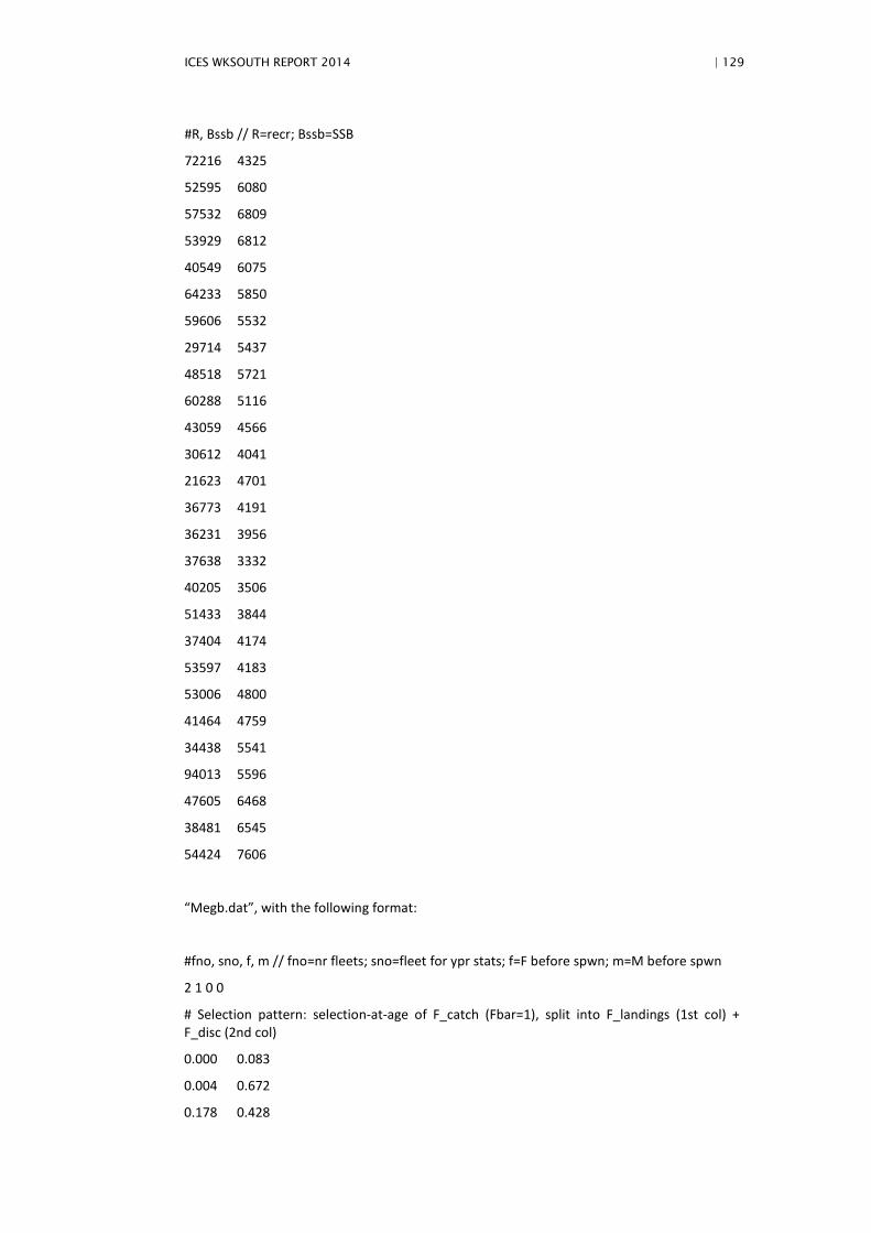
ICES WKSOUTH REPORT 2014 | 129
#R, Bssb // R=recr; Bssb=SSB
72216 4325
52595 6080
57532 6809
53929 6812
40549 6075
64233 5850
59606 5532
29714 5437
48518 5721
60288 5116
43059 4566
30612 4041
21623 4701
36773 4191
36231 3956
37638 3332
40205 3506
51433 3844
37404 4174
53597 4183
53006 4800
41464 4759
34438 5541
94013 5596
47605 6468
38481 6545
54424 7606
“Megb.dat”, with the following format:
#fno, sno, f, m // fno=nr fleets; sno=fleet for ypr stats; f=F before spwn; m=M before spwn
2 1 0 0
# Selection pattern: selection-at-age of F_catch (Fbar=1), split into F_landings (1st col) + F_disc (2nd col)
0.000 0.083
0.004 0.672
0.178 0.428

130 | ICES WKSOUTH REPORT 2014
0.674 0.257
1.385 0.078
1.787 0.033
1.503 0.014
1.513 0.004
# cv Selection pattern
0.175 0.175
0.175 0.175
0.097 0.097
0.076 0.076
0.079 0.079
0.085 0.085
0.109 0.109
0.109 0.109
# Weight at age
0.003 0.005
0.037 0.021
0.067 0.040
0.086 0.053
0.107 0.083
0.139 0.120
0.178 0.148
0.247 0.114
# cv Weight at age
0.112 0.255
0.112 0.255
0.143 0.282
0.137 0.419
0.097 0.542
0.062 0.480
0.050 0.345
0.040 0.792
# Biological data
# M, mat, wSSB
0.2 0 0.005
0.2 0.55 0.021
0.2 0.86 0.049
0.2 0.97 0.077

ICES WKSOUTH REPORT 2014 | 131
0.2 0.99 0.106
0.2 1 0.138
0.2 1 0.178
0.2 1 0.247
# cv Biological data
# cvM, cvmat, cvwSSB
0.1 0.0 0.112
0.1 0.1 0.112
0.1 0.1 0.143
0.1 0.1 0.137
0.1 0.1 0.097
0.1 0.0 0.062
0.1 0.0 0.050
0.1 0.0 0.040
While preparing the “Megb.dat” file, it was noted that the fish are assumed to mature really young: 55% of the fish mature at age 1. Given that the mean weight of the age 1 fish is only 21 g, this seems a very low age and weight of maturation. This maturity assumption is also made in the assessment. It is recommended that it is checked by the appropriate scientists with their colleagues in their home institutes.
From the “Megb.dat” file, it can be also be seen that there is high selection of fish at ages 1 and 2, which are then largely discarded. This selection of small fish, which are subsequently mainly discarded, is expected to have a clear impact on calculated FMSY values (obtained by maximizing long-term yield = landings) resulting in lower FMSY values.
Figure 5.5.6.1. Four-spot megrim: selection-at-age (F(a)/F(2-4)) of total catch, obtained as an arith-metic (red) or geometric (blue) mean of 2008-2012.
0.000
0.500
1.000
1.500
2.000
0 2 4 6 8
Selection-at-age: mean 2008-2012

132 | ICES WKSOUTH REPORT 2014
Figure 5.5.6.2. Four-spot megrim: weight-at-age (for calculation of SSB and total catch in weight) for each historic year and average of 2008-2012 (red dots)
Results
The “plotMSY” function from the R “msy” library was run with 1000 iterations. The three stock–recruitment relationships provided in the software (Ricker, Beverton–Holt, Hockey-stick) were tried. The software produces results for each of them sepa-rately. It also allows to combine them (in a bootstrap-type way) assigning user-selected weights to each of them (based on biological/ecosystem knowledge of what is more appropriate to the stock in question) or automatic weights based on their re-spective likelihood fits to the stock-recruitment “data”. In the automatic weighting option, some trimming is required to get stable weights (0.5% trimming was applied for the four-stock megrim stock after an initial run with no trimming and following the exploratory procedure suggested in Annex 7 of the WGMG 2013 report).
Figures 5.5.6.3-7 show the results for each of the stock-recruitment functions and a per-recruit analysis.
0
0.1
0.2
0.3
0.4
0 2 4 6 8
Weight-at-age in stock

ICES WKSOUTH REPORT 2014 | 133
Figure 5.5.6.3. Four-spot megrim: stock-recruitment pairs from assessment (open circles) and fits from Ricker, Beverton–Holt and Hockey-stick functions.

134 | ICES WKSOUTH REPORT 2014
Figure 5.5.6.4. Four-spot megrim: results for Ricker stock-recruitment function.

ICES WKSOUTH REPORT 2014 | 135
Figure 5.5.6.5. Four-spot megrim: results for Beverton–Holt stock-recruitment function.

136 | ICES WKSOUTH REPORT 2014
Figure 5.5.6.6. Four-spot megrim: results for Hockey-stick stock-recruitment function.

ICES WKSOUTH REPORT 2014 | 137
Figure 5.5.6.7. Four-spot megrim: results for per-recruit analysis.

138 | ICES WKSOUTH REPORT 2014
Results in table form were also obtained for each stock-recruit function considered, per-recruit, and with automatic (likelihood-based) weighting of the three stock-recruitment functions (weights in table given in the order Ricker, Beverton–Holt, Hockey-stick).
Table 5.5.6.1. Four-spot megrim: results per-recruit, for each stock-recruitment function separately, and with equal (first 4 columns of final rows) automatic (last 4 columns of final rows) weighting.
Stock name
Megb Sen filename
NA
index filename
NA
Number of iterations
1000
Simulate variation in Biological parameters
TRUE
SR relationship constrained
TRUE
Ricker
1000/1000 Iterations resulted in feasible parameter estimates
Fcrash Fmsy Bmsy MSY ADMB Alpha ADMB Beta Unscaled Alpha Unscaled Beta AICc
Deterministic 0.63 0.18 9770 1679 1.07 0.48 16.08 0.00 15.98
Mean 0.61 0.18 13337 2184 1.09 0.51 17.33 0.00 18.05
5%ile 0.34 0.13 6263 1330 0.97 0.15 10.84 0.00 16.09
25%ile 0.47 0.16 7545 1486 1.03 0.36 13.96 0.00 16.63
50%ile 0.58 0.18 8966 1660 1.08 0.51 16.58 0.00 17.53

ICES WKSOUTH REPORT 2014 | 139
75%ile 0.72 0.20 12155 1992 1.14 0.66 20.08 0.00 18.90
95%ile 0.99 0.24 25142 3731 1.21 0.90 26.16 0.00 21.82
CV 0.32 0.19 2.21 1.56 0.07 0.43 0.28 0.43 0.11
N 1000 1000 1000 1000 1000 1000 1000 1000 1000
Beverton–Holt
1000/1000 Iterations resulted in feasible parameter estimates
Fcrash Fmsy Bmsy MSY ADMB Alpha ADMB Beta Unscaled Alpha Unscaled Beta AICc
Deterministic 0.84 0.13 15416 2002 0.50 0.93 80083.50 3744.93 15.95
Mean 0.93 0.12 34681 3884 0.49 0.95 195641.52 17386.61 17.78
5%ile 0.35 0.09 8603 1422 0.14 0.85 49310.20 444.38 16.08
25%ile 0.50 0.11 11421 1674 0.34 0.90 62746.23 1939.17 16.50
50%ile 0.71 0.12 14773 1985 0.50 0.94 80622.60 3883.65 17.27
75%ile 1.08 0.14 21213 2561 0.64 0.99 118881.25 8185.11 18.44
95%ile 2.38 0.16 48623 5376 0.81 1.06 284914.25 26284.52 21.15
CV 0.74 0.17 9.57 8.12 0.42 0.07 9.72 13.38 0.10
N 962 1000 1000 1000 1000 1000 1000 1000 1000
Smooth hockeystick
1000/1000 Iterations resulted in feasible parameter estimates
Fcrash Fmsy Bmsy MSY ADMB Alpha ADMB Beta Unscaled Alpha Unscaled Beta AICc
Deterministic 0.38 0.17 10020 1603 0.53 0.99 4.94 5111.63 16.89
Mean 0.36 0.17 9390 1623 0.57 0.96 5.28 4951.88 18.97
5%ile 0.26 0.15 7129 1327 0.47 0.69 4.36 3556.35 17.16
25%ile 0.31 0.16 8366 1477 0.51 0.81 4.76 4195.76 17.66
50%ile 0.36 0.17 9224 1601 0.55 0.94 5.12 4877.13 18.43
75%ile 0.41 0.17 10326 1738 0.62 1.07 5.69 5553.60 19.68

140 | ICES WKSOUTH REPORT 2014
95%ile 0.50 0.19 12168 2021 0.72 1.34 6.63 6908.86 22.35
CV 0.21 0.07 0.16 0.13 0.13 0.20 0.13 0.20 0.10
N 1000 1000 1000 1000 1000 1000 1000 1000 1000
Per recruit
F20 F25 F30 F35 F40 F01 Fmax Bmsypr MSYpr
Deterministic 0.33 0.26 0.21 0.17 0.14 0.11 0.17 0.20 0.03
Mean 0.31 0.24 0.19 0.16 0.13 0.11 0.17 0.18 0.03
5%ile 0.25 0.20 0.16 0.13 0.11 0.09 0.15 0.15 0.03
25%ile 0.28 0.22 0.18 0.15 0.12 0.10 0.16 0.17 0.03
50%ile 0.31 0.24 0.19 0.16 0.13 0.11 0.17 0.18 0.03
75%ile 0.34 0.26 0.21 0.17 0.14 0.11 0.17 0.20 0.03
95%ile 0.38 0.29 0.23 0.19 0.15 0.12 0.19 0.22 0.04
CV 0.12 0.11 0.11 0.11 0.10 0.08 0.07 0.12 0.06
N 1000 1000 1000 1000 1000 1000 1000 1000 1000
Combining all SRRs
Automatically specified weights
0.34 0.42 0.24
Percentage Fmsy Fcrash MSY Bmsy Fmsy_w Fcrash_w MSY_w Bmsy_w
5% 0.10 0.28 1343 6790 0.10 0.28 1355 6877
25% 0.13 0.37 1514 8505 0.12 0.39 1513 8592
50% 0.16 0.50 1692 10088 0.15 0.53 1724 10592
75% 0.18 0.71 2037 13754 0.17 0.74 2133 15320
95% 0.22 1.37 3792 31545 0.21 1.52 3976 33452

ICES WKSOUTH REPORT 2014 | 141
The stock-recruitment values obtained from the assessment do not show any clear stock-recruitment signal to allow a clear estimation of a stock-recruitment curve (Figure 5.5.6.3). The time-series is relatively short and there are no data sufficiently close to the origin to allow an un-derstanding of what may happen at lower stock biomasses. Based on the available data, there is no indication that recruitment might decrease at high stock sizes (which would be typical of a Ricker curve).
It is noted that the estimated recruitment (age 0) is strongly dependent on the time-series of dis-cards (introduced for the first time in the assessment at this benchmark). The discard time-series is highly uncertain before 1994, as there are no discard observations from that early period (dis-cards each year were reconstructed using the observed mean values, from the years with discard sampling, during 1995-1999); this also results in high uncertainty in recruitment estimates.
Despite all these issues, the range of values that were generally found to be consistent with high long-term yield is not very wide, as can be seen from Table 5.5.6.1. FMSY would be 0.12 based on Beverton–Holt, 0.17 based on Hockey-stick, and 0.18 based on Ricker. During the last decade, the SSB has been continuously increasing, and it is now estimated to be at its historical maximum. During the same period, F has shown a clear decreasing trend, from about 0.4 at the start of the period to 0.23 in 2011, and then dropping to 0.14 in 2012. The historical stock development sug-gests that F values not exceeding approximately 0.3 are sustainable and allow clear stock increas-es. At the same time, the high fishery selection and discarding at ages 1 and 2 causes the yield-per-recruit curve to peak at a low F value (Fmax = 0.17).
Based on all of the above, Fmax = 0.17 is considered an appropriate FMSY proxy for the stock.
The WKMSYREF2 report notes that if Fmax is chosen as a proxy for FMSY, a test for precautionary considerations should be made. The arguments provided in the paragraph above indicate that fishing at F=0.17 should be precautionary for this stock. An additional test was done with Plot-MSY as follows:
As part of the PlotMSY output, a plot of the estimated long-term probability of SSB<Blim, when fishing at a constant F is produced. Either 3300 t (Bloss=SSB2001) or 3800 t (excluding the two lowest SSB values, for which recruitment was a bit below the long-term historic average), could be con-sidered as Blim candidates. Based on the CVs specified in the “Megb.dat” file and the automatic weighting of the three stock-recruitment functions, long-term fishing at a constant F=0.26 gives a 5% probability of long-term SSB < 3300 t (Figure 5.5.6.8), whereas long-term fishing at a constant F=0.25 gives a 5% probability of long-term SSB < 3800 t (no figure shown). This provides another indication that fishing at F=0.17 should be precautionary for this stock. It must be stressed that the CVs used in this analysis were simply taken from the example provided with PlotMSY (corre-sponding to North Sea cod). This probability plot should be done with CVs that are carefully thought about and considered appropriate to the four-spot megrim stock. There was no time to consider this at the benchmark, but at least the analysis at the benchmark shows some robustness of the F=0.17 against some degree of uncertainty.

142 | ICES WKSOUTH REPORT 2014
Figure 5.5.6.8. Four-spot megrim: long-term probability of SSB < Blim (for this plot, Blim is taken as 3300 t)
The ICES MSY harvest control rule is based on fishing at FMSY if SSB ≥ MSY Btrigger and applying a linear reduction in F when SSB < MSY Btrigger. For most stocks, MSY Btrigger has been initially set at Bpa. For the four-spot megrim stock, a provisional choice of biomass reference points could thus be: Blim=3300 t (=Bloss, based on no signal of impaired recruitment during the historical time-series); Bpa = 4600 t (default choice Bpa = 1.4 Blim); MSY Btrigger = 4600 t (default choice = Bpa). It must be stressed once more that the short time available during the benchmark did not permit a careful consideration of these potential biomass reference points. Therefore, they are simply noted here as potential values that should merit further consideration by the assessment working group (WGBIE).
Conclusions and recommendations
• The little time available during the benchmark did not permit very careful considera-tion of reference points, so the results derived during the benchmark should be further considered during the assessment working group (WGBIE). This is particularly the case for the biomass reference points. Fmax (= 0.17 with the settings used in this report section) is suggested as FMSY proxy for the stock (to be further considered by WGBIE). A preliminary run with geometric mean (of 2008-2012) instead of arithmetic mean for selection-at-age gives Fmax as 0.18. When WGBIE carefully reconsiders the analysis in this section, it is suggested that the geometric mean is used for selection-at-age, as discussed during the benchmark meet-ing (and already incorporated in the reference points section for megrim).
• Potential biomass reference points were also suggested at the benchmark (to be further considered by WGBIE)
• It is recommended that additional exploration of model settings and sensitivities (e.g. CVs used in the “Megb.dat” file; the high uncertainty in recruitment before 1994 be-cause of the discard estimates used for that early period) is conducted.
• Check the maturity assumption at age 1 used in the assessment and reference points analysis.
• Before making final decisions on reference points for four-spot megrim, the potential reference points for megrim also need to be considered, as there is a single TAC for
O:\ADVISORY SERVICES\ACOM\Expert Groups\Benchmark Groups\WKSOUTH\2014\WKSOUTH13.Docx

ICES WKSOUTH REPORT 2014 | 143
both species. The benchmark did not have time to consider any aspect in relation to this. There was almost no time at the benchmark to consider potential reference points for megrim.
Work conducted after benchmark meeting
The work presented here used the latest version of the “msy” package available on the GITHUB site on February 13, 2014. This is msy package version 0.1.12.
The analysis was expanded after the benchmark meeting ended, in three ways as follows:
First, the same analysis presented here was rerun using the geometric mean (instead of the arithmetic mean) of years 2008-2012 for the selection-at-age of the catch. This was agreed during the benchmark meeting, as recommended and done as well for megrim (L. whiffiagonis). This change produced very slightly higher (median) values of the potential reference points: Fmax=0.18 (close to F35%=0.17), whereas FMSY was 0.19, 0.13, and 0.18, under Ricker, Beverton–Holt and Hock-ey-stick, respectively. Values of F below 0.27 correspond to less than 5% long-term probability of SSB being below 3300 t (Bloss), based on the likelihood weighting of the three stock-recruitment functions automatically done by the PlotMSY software.
Second, the analysis just explained (based on geometric mean) was redone, changing the CVs to those corresponding to the four-spot megrim assessment assumptions (in the case of weight, M and proportion mature at age) or assessment results (in the case of selection at age) for the last 5 years (2008-2012). Based on these CVs, there are, once again, some slight changes to the (median) values of potential reference points: Fmax=0.18 (equal to F35%=0.18), whereas FMSY was 0.20, 0.13, and 0.18, under Ricker, Beverton–Holt and Hockey-stick, respectively. Values of F below 0.33 cor-respond to less than 5% long-term probability of SSB being below 3300 t (Bloss), based on the like-lihood weighting of the three stock-recruitment functions.
Third, the EqSim software (also developed at the 2014 ICES workshop WKMSYREF2 and includ-ed in the “msy” package) was also applied. Inputs for (at age) fishery selection, proportion land-ed and discarded, weight, M and proportion mature were randomly drawn from the four-spot megrim assessment assumptions (in the case of weight, M and proportion mature at age) or as-sessment results (in the case of selection at age) for the last 5 years (2008-2012). The Ricker, Beverton–Holt and Hockey-stick SR relationships were considered; it must be noted that the EqSim software estimated different weights for each of these SR relationships than the PlotMSY software. Long-term projections, including the randomly drawn parameters noted above and annual stochastic variability of recruitment, were conducted for different F values. A graphical display of results is presented in Figure 5.5.6.9. The figure shows a fairly flat yield (long-term landings) curve, with a maximum at F=0.16, whereas values of F below 0.36 give less than 5% long-term probability of SSB being below 3300 t (Bloss, which could be considered a candidate for Blim). Following the guidelines in Section 4.3 of the WKMSYREF2 report, a test was then conduct-ed incorporating assessment and implementation error in the long-term projections (this was done simply, assuming that the real F in each projection year varied stochastically around the intended F with the errors having CV=0.25 and 0.3 correlation between consecutive years). By introducing these errors in the realized F, the “intended” F value giving 5% probability of SSB being less than 3300 t decreased to F=0.34 (from the previous 0.36, calculated without errors in realized F). Finally, repeating the latter exercise for the ICES MSY HCR (which, when SSB < MSY Btrigger, reduces F linearly from the target F), assuming MSY Btrigger = 1.4*3300 t, the target F value giving 5% probability of SSB being less than 3300 t increased to F=0.41.

144 | ICES WKSOUTH REPORT 2014
Figure 5.5.6.9. Four-spot megrim, long-term projections from EqSim including stochastic annual recruitment: (a) recruitment vs. F, (b) SSB vs. F, (c) yield (i.e. landings) vs. F, (d) probability of SSB < Blim and Bpa vs. F (for this plot it is assumed Blim=3300 t, and Bpa=1.4 Blim). In all panels, the green vertical line is at F=0.36 (the F value that gives 5% probability of SSB < Blim). The left-most vertical line in panel (c) is at F=0.16 (the F value that maximiz-es long-term average landings). Historical estimates from the benchmark assessment are represented as dots in panels (a), (b), (c).
Taking all the above information into account, as well as the historic stock development as esti-mated by the benchmark assessment, the following reference points are proposed:
Blim = 3300 t (provisional reference point; Bloss in the 2014 benchmark assessment),
Bpa = 4600 t (default option;1.4 Blim),
MSY Btrigger = 4600 t (default option; Bpa),
FMSY=0.18 (Fmax as FMSY proxy; a check for precautionary considerations has been conducted).
Given the uncertainties surrounding the recruitment estimates (due to uncertain discards esti-mates), these reference points should be considered provisional. They represent pragmatic choic-es given the current state of knowledge.
It is recommended that the assessment working group WGBIE gives further consideration to these proposals.
5.5.7 Future Research and data requirements
Develop more appropriate tuning fleets which cover the full spatial extent of the stock.
Gather and evaluate additional commercial information such as the Coruña and Avilés time-series and combine these time-series into appropriate tuning indices.
O:\ADVISORY SERVICES\ACOM\Expert Groups\Benchmark Groups\WKSOUTH\2014\WKSOUTH13.Docx

ICES WKSOUTH REPORT 2014 | 145
Migrate the assessment models from XSA to the SAM statistical catch-at-age model. This increas-es the flexibility of the modelling approach (e.g. it removes the assumption of exact catches) and is in line with many other stocks within ICES
The reference point model for megrim and four spot megrim needs further exploration.
Given the issues highlighted at this benchmark, work should be conducted towards a better method of incorporating discarding into the assessment
Evaluate the validity of the maturity-at-age 1 value (for both stocks, but particularly for four-spot megrim)
Explore removal of age 0 from the assessment and evaluate the impact on catch recommenda-tions

146 | ICES WKSOUTH REPORT 2014
6 References
Abad, E., Bellido, J.M. y A. Punzón, 2010. Transfer of fishing effort between areas and fishery units in Span-ish fisheries as side effects of the Prestige oil spill management measures. Ocean and Coastal Manage-ment, 53:107-113.
Álvarez-Salgado, X.A., Beloso, S., Joint, I., Nogueira, E., Chou, L., Pérez, F.F., Groom, S., Cabanas, J.M., Rees, A.P., Elskens, M., 2002. New production of the NW Iberian shelf during the upwelling season over the period 1982–1999. Deep-Sea Research, I 49, 7 1725–1739.
Bailey, K. M. 1994. Predation on juvenile flatfish and recruitment variability. Netherlands Journal of Sea Research, 32: 175–189.
Beverton, R. J. H., and Iles, T. C. 1992. Mortality rates of 0-group plaice (Pleuronectes platessa L.), dab (Liman-da limanda L.) and turbot (Scophthalmus maximus L.) in European waters III. Density-dependence of mor-tality rates of 0-group plaice and some demographic implications. Netherlands Journal of Sea Research, 29: 61–79.
BIOSDEF. 1998. Biological studies of demersal fish. Ref.: EU, DG XIV, Study Contract 95/038.
Castro, J., Marín, M., Costas, G., Abad, E., Punzón, A., Pereiro, J. y Vázquez, A. 2011. ATLAS de las flotas de pesca españolas de aguas europeas atlánticas. Temas de Oceanografía, nº 4. Instituto Español de Ocea-nografía. Ministerio de Ciencia e Innovación. 215 pp.
Gibson R. N., 1994. lmpact of habitat quality and quantity on the recruitment of juvenile flatfishes. Nether-lands Journal of Sea Research 32:191-206
Danancher, D. and E. García-Vázquez, 2009. Population differentiation in megrim (Lepidorhombus whiffag-onis) and four spotted megrim (Lepidorhombus boscii) across Atlantic and Mediterranean waters and im-plications for wild stock management. Marine Biology (2009) 156:1869–1880.
Landa, J., Piñeiro, C., and Pérez, N. 1996. Megrim (Lepidorhombus whiffiagonis) growth patterns in the north-east Atlantic. Fisheries Research, 26: 279–294.
Landa, J., 1999. Density-dependent growth of four spot megrim (L. boscii) in the northern Spanish shelf. Fisheries Research, 40: 267-276.
Landa, J. and C. Piñeiro, 2000. Megrim (Lepidorhombus whiffiagonis) growth in the North-eastern Atlantic based on back-calculation of otolith rings. ICES Journal of Marine Science, 57: 1077–1090.
Landa J, Perez N, and C. Pineiro, 2002. Growth patterns of the four spot megrim (Lepidorhombus boscii) in the northeast Atlantic. Fisheries Research, 55 (1-3): 141-152.
Pérez N., J. Santos, H. Araújo and I. Salinas, 2011. Southern Megrim Species Results from Spanish Discard Sampling Programme. WD to WGHMM11.
Punzón, A., C. Hernández, E. Abad, J. Castro, N. Pérez and V. Trujillo, 2010. Spanish otter trawl fisheries in the Cantabrian Sea. – ICES Journal of Marine Science 67: 1604–1616
Rodriguez-Marín, E. and Olaso, I. 1993. Food composition of the two species of megrim (Lepidorhombus whiffiagonis and Lepidorhombus boscii) in the Cantabrian Sea. Actes du IIIème Colloque d’Oceanographie du Golfe de Gascogne. Arcachon 1992: 215–219
Rodríguez-Marín E., A. Serrano y F. Velasco, 2002. Diferenciación trófica de las dos especies de gallo del Cantábrico respecto a los crustáceos decápodos. XII Simposio Ibérico de Estudios del Bentos Marino Abstracts Book. Gibraltar-La Línea de la Concepción, Spain.
Sánchez, F. and Gil, J. 1995. Influencia de anomalías térmicas de mesoscala sobre la distribución de peces demersales. Actes du IVème Colloque d’Oceanographie du Golfe de Gascogne. Santander 1994: 49–54
O:\ADVISORY SERVICES\ACOM\Expert Groups\Benchmark Groups\WKSOUTH\2014\WKSOUTH13.Docx

ICES WKSOUTH REPORT 2014 | 147
Sánchez, F., Pérez, N. and J. Landa, 1998. Distribution and abundance of megrim (Lepidorhombus boscii and Lepidorhombus whiffiagonis) on the northern Spanish shelf. ICES Journal of Marine Science, 55: 494–514
Sánchez, F., Blanco, M. and R. Gancedo, 2002. Atlas de los peces demersales y de los invertebrados de inte-rés comercial de Galicia y el Cantábrico otoño 1997-1999. 158 pp. [ISBN 84-95877-02-3].
Serrano, A., Preciado, I., Abad, E, Sánchez, F., Parra, S. and I. Frutos, 2008. Spatial distribution patterns of demersal and epibenthic communities on the Galician continental shelf (NW Spain). Journal of Marine Systems, 72: 87–100.
Van der Veer, H. W., Pihl, L., and Bergman, M. J. N., 1990. Recruitment mechanisms in North Sea plaice Pleuronectes platessa. Marine Ecology Progress Series, 64: 1–12.
Van der Veer HW, Berghahn R, Miller JM, Rijnsdorp AD, 2000. Recruitment in flatfish, with special empha-sis on North Atlantic species: Progress made by the Flatfish Symposia. ICES Journal of Marine Science, 57:202-215.
Wennhage, H. and L. Pihl. 2001. Settlement patterns of newly settled plaice (Pleuronectes platessa) in a non-tidal Swedish fjord in relation to larval supply and benthic predators. Marine. Biology, 139: (5) 877–889.
Belloc, G. 1935. Etude monographique du merlu Merluccius merluccius L., 3ème partie. Revue des Travaux de l’Office des Pêches maritimes, 8: 145e202.
de Pontual, H., Bertignac, M., Battaglia, A., Bavouzet, G., Moguedet, P., and Groison, A.-L. 2003. A pilot tagging experiment on European hake (Merluccius merluccius): methodology and preliminary results.
de Pontual, H., Jolivet, A., Garren, F., and Bertignac, M. 2013. New insights on European hake biology and population dynamics from a sustained tagging effort in the Bay of Biscay. ICES Journal of Marine Sci-ence: Journal du Conseil, 70: 1416-1428.
García-Vázquez, E., Izquierdo, J. and J. Pérez, 2006. Genetic variation at ribosomal genes supports the exist-ence of two different European subspecies in the megrim Lepidorhombus whiffiagonis. Journal of Sea Re-search, 56: 59–64.
Hewitt, D.A. and JM. Hoenig. 2005 Comparison of two approaches for estimating natural mortality based on longevity. Fish Bull 103: 433–437.
Hickling C. F. Fisheries Investigations Series 2. Vol. 13.(2) 1933. The natural history of hake. 4. Age determi-nation and growth rate. UK Ministry of Agriculture, Fisheries and Food. 120 pp.
Hui-Hua Lee, Kevin R. Piner, Richard D. Methot Jr., Mark N. Maunder. 2014. Use of likelihood profiling over a global scaling parameter to structure the population dynamics model: An example using blue marlin in the Pacific Ocean. Fisheries Research (in press 2014)
ICES Journal of Marine Science: Journal du Conseil, 60: 1318-1327.de Pontual, H., Groison, A. L., Pineiro, C., and Bertignac, M. 2006. Evidence of underestimation of European hake growth in the Bay of Biscay, and its relationship with bias in the agreed method of age estimation. 10.1016/j.icesjms.2006.07.007. ICES J. Mar. Sci., 63: 1674-1681.
ICES 2010a. Report of the Workshop on Age estimation of European hake (WKAEH), 9–13 November 2009, Vigo, Spain. ICES , CM 2009/ACOM:42: 67 pp.
ICES 2010b. Report of the Benchmark Workshop WKROUND, 9–16 February 2010, Copenha- gen, Denmark. ICES.
Piñeiro, C., Rey, J., de Pontual, H., and Goñi, R. 2007. Tag and recapture of European hake (Merluccius mer-luccius L.) off the Northwest Iberian Peninsula: First results support fast growth hypothesis. Fisheries Research, 88: 150-154.

148 | ICES WKSOUTH REPORT 2014
Annex 1: New stock annexes
Stock Annex Northern Stock of Hake
Stock specific documentation of standard assessment procedures used by ICES.
Stock Northern Stock of Hake (Division IIIa, Subareas IV, VI and VII and Divisions VIIIa,b,d)
Working Group: Working Group for the Bay of Biscay and Iberic Waters Ecoregion (WGBIE)
Date: 1 April 2014
Revised by WKSOUTH2014
A. General
A.1. Stock definition
European hake (Merluccius merluccius) is widely distributed over the Northeast Atlantic shelf, from Norway to Mauritania, with a larger density from the British Islands to the south of Spain (Casey and Pereiro, 1995) and in the Mediterranean and Black sea. Although, as demonstrated by genetic studies (Plá and Roldán, 1994; Roldán et al., 1998), there is no evidence of multiple popu-lations in the Northeast Atlantic, ICES assumes since the end of the 1970s two different stock units: the so called Northern stock, in Division IIIa, Subareas IV, VI and VII and Divisions VIIIa,b,d, and the Southern stock in Divisions VIIIc and IXa, along the Spanish and Portuguese coasts. The main argument for this choice was that the Cap Breton canyon (close to the border between the Southern part of Division VIIIb and the more Eastern part of Division VIIIc, i.e. ap-proximately between the French and Spanish borders) could be considered as a geographical boundary limiting exchanges between the two populations.
Hake spawn from February through to July along the shelf edge, the main areas extending from the north of the Bay of Biscay to the south and west of Ireland (Figure 1). After a pelagic life, 0-group hakes reach the bottom in depths of more than 200 m, then moving to shallower water with a muddy seabed (75–120 m) by September. There are two major nursery areas: in the Bay of Biscay and off southern Ireland.
O:\ADVISORY SERVICES\ACOM\Expert Groups\Benchmark Groups\WKSOUTH\2014\WKSOUTH13.Docx

ICES WKSOUTH REPORT 2014 | 149
Figure 1. Main spawning and nursery areas. Spawning areas sloping downwards from left to right; Nursery areas sloping downwards from right to left. (from Casey and Pereiro, 1995)
A.2. Fishery
A set of different Fishery Units (FU) has been defined by the ICES Working Group on Fisheries Units in Sub-areas VII and VIII in 1985, in order to study the fishing activity related to demersal species (ICES, 1991a). To take into account the hake catches from other areas, a new Fishery Unit was introduced at the beginning of the nineties (FU 16: Outsiders). This Fishery Unit was created on the basis of combination between mixed areas and mixed gears (trawl, seine, longline, and gillnet). The current FU are defined as follows:
Fishery Unit Description Sub-area
FU1 Longline in medium to deep water VII
FU2 Longline in shallow water VII
FU3 Gillnets VII
FU4 Non-Nephrops trawling in medium to deep water VII
FU5 Non-Nephrops trawling in shallow water VII
FU6 Beam trawling in shallow water VII
FU8 Nephrops trawling in medium to deep water VII
FU9 Nephrops trawling in shallow to medium water VIII
FU10 Trawling in shallow to medium water VIII
FU12 Longline in medium to deep water VIII
FU13 Gillnets in shallow to medium water VIII
FU14 Trawling in medium to deep water VIII
FU15 Miscellaneous VII & VIII
FU16 Outsiders IIIa, IV, V & VI
FU00 French unknown

150 | ICES WKSOUTH REPORT 2014
The main part of the fishery is currently conducted in six Fishery Units, three of them from Sub-area VII: FU 4, FU 1 and FU 3, two from Subarea VIII: FU 13 and FU 14 and one in Subareas IIIa, IV, V and VI : FU16.
From the information reported to the Working Group, Spain accounted in recent years for the main part of the landings (around 43%) followed by France (around 29%), UK, Denmark, Ireland, Norway, Belgium, Netherlands, Germany, and Sweden contributing to the remaining.
The minimum landing size for fish caught in Subareas IV, VI, VII and VIII is set at 27 cm total length (30 cm in Division IIIa).
From 14th of June 2001, an Emergency Plan was implemented by the Commission for the recov-ery of the Northern hake stock (Council Regulations N°1162/2001, 2602/2001 and 494/2002). In addition to a TAC reduction, 2 technical measures were implemented:
A 100 mm minimum mesh size has been implemented for otter trawlers when hake comprises more than 20% of the total weight of marine organisms retained on board. This measure did not apply to vessels less than 12 m in length and which return to port within 24 hours of their most recent departure.
Two areas have been defined, one in Subarea VII and the other in Subarea VIII, where a 100 mm minimum mesh size is required for all otter trawlers, whatever the amount of hake caught.
Council Regulation (EC) No. 1954/2003 established measures for the management of fishing effort in a biologically sensitive area in Subareas VIIb, VIIj, VIIg, and VIIh. Effort exerted within the biologically sensitive area by the vessels of each EU Member State may not exceed their average annual effort (calculated over the period 1998–2002).
There are explicit management objectives for this stock under the EC Reg. No 811/2004 imple-menting measures for the recovery of the northern hake stock. It is aiming at increasing the quan-tities of mature biomass to values equal to or greater than 140 000 t. This is to be achieved by limiting fishing mortality to 0.25 and by allowing a maximum change in TAC between years of 15%.
According to ICES in 2007, the northern hake stock has met the SSB target in the recovery plan of 140 000 t for two consecutive years (2006 and 2007). Article 3 of the recovery plan indicates that, in such a situation, a management plan should be implemented.
An annual one-month fishing activity stop has been implemented by the Spanish administration since 2004. In 2008, a specific national regulation established a 90-days stop to be distributed from August 2008 to December 2009.
In Subarea VIII, for 2006, 2007 and 2008, otter trawlers using a square mesh panel are allowed to use 70 mm mesh size in the area, mentioned above, where 100 mm minimum mesh size is re-quired for all otter trawlers. (EC Reg. No. 51/2006; EC Reg. 41/2007).
Furthermore, there was a ban on gillnets in Divisions VIa,b and VIIb,c,j,k fishing at more than 200 m of depth (EC Reg. No 51/2006) during the first semester of 2006.
A.3. Ecosystem aspects
Although a comprehensive study on the role of hake in its ecosystem has not yet been carried out, some partial studies are available. Hake belongs to a very extended and diverse community of commercial species including megrim, anglerfish, Nephrops, sole, sea bass, ling, blue ling,
O:\ADVISORY SERVICES\ACOM\Expert Groups\Benchmark Groups\WKSOUTH\2014\WKSOUTH13.Docx

ICES WKSOUTH REPORT 2014 | 151
greater forkbeard, tusk, whiting, blue whiting, Trachurus spp, conger, pout, cephalopods (octo-pus, Loligidae, Ommastrephidae and cuttlefish), and rays. The relative importance of these species in the hake fishery varies largely in relation to the different gears, sea areas, and countries in-volved.
Hake is preyed upon by sharks and other fish. Cannibalism on juveniles by adults is also quoted. Adults feed on fish (mainly on blue whiting and other gadoids, sardine, anchovy, and other small pelagic fish); juvenile hake prey mainly upon planktonic crustaceans (above all euphausids, co-pepods, and amphipods).
Ecological factors or environmental conditions impacting on hake population dynamics are not taken into account at present in the assessment or in the management. However, synchronous changes have been observed in hake recruitment success and several global, regional and local parameters, which suggest that environmental conditions may be influential for hake (Goikoetx-ea and Irigoien, 2013). An ecological regime shift occurred in the Northeast Atlantic shelf system in 1988/89, which was detected at global scale (NAO, Gulf Stream and northern hemisphere tem-perature anomaly), as well as regionally (climatology of the Northeast Atlantic and copepod var-iability of the Celtic Sea). The region went from a period of cool temperatures and relatively weak wind (1978-1989) to a period of warmer temperatures and stronger westerly winds (1900-2006). Given the synchronous stepwise increase in hake recruitment success, it was concluded that the environment shifted to a regime that was favourable for northern hake. Early life stages of hake were found to benefit from a warming trend (either through the widening of the optimal envi-ronmental window or/and higher growth rates). In addition, coastward transport avoided vul-nerable stages from their dispersion to oceanic areas and helped in their transport from spawning areas to nursery grounds (Goikoetxea, 2011). Other previous studies also highlighted the influ-ence of environmental parameters such as water temperature and wind-driven transport on northern hake stock (Fernandes et al., 2010; Álvarez et al., 2001).
B. Data
In 2013 a data call was run by ICES in order to obtain more precise data on discards since 2003. Discard and Landing data were uploaded into InterCatch by most of the countries that exploit the stock. The disaggregation level varied by country and year, from season, métier and length disaggregation level to total landings or discards by year.
B.1. Commercial catch B.1.1. Landings
Until 2010, the Spanish landings data were based on sales notes and Owners Associations records compiled by the National laboratories (IEO and AZTI). From 2011, the Spanish data are derived from official statistics provided by the Spanish Fishery Administration. French landings data are based on logbook and auction hall sales.
From 1978 to 1989, landings in weight are available by year, gear (trawl, gillnets and longline), country (UK, France and Spain) and ICES Divisions (Division IVa + Sub-Area VI, Division VII and Divisions VIII a+b). From 1990 to present, for most of the years, landings in weight by FUs and countries are available on a quarterly basis. In 1992, only data from Spain is available by FU and on a quarterly basis (Table 1).

152 | ICES WKSOUTH REPORT 2014
Table 1. Landings-in-weight (and their level of aggregation) available to the Working Group.
1978 to 1989 1990-1991 1992 1993 to Present
By Gear, Country and ICES Divisions X
By FU X X X
By year X X
By quarter X X* X
* For Spain only
From 1978 to 1989, length–frequency distributions are available by year, gear, country and ICES Divisions. From 1990 to present, length compositions of the landings are not available for all Fishery Units, quarters and countries. Only the main FUs/Countries are sampled. Table 2 pre-sents, as an example, the length distributions available for 2008.
Table 2. Length–frequency distributions provided to the Working Group in 2008.
FU France Ireland Spain UK(EW) Scotland Danemark
01 Quarterly
03 Quarterly Quarterly Quarterly
04 Quarterly Quarterly
05 Quarterly Quarterly
06 Quarterly
09 Quarterly
10 Quarterly
12 Quarterly Quarterly
13 Quarterly Quarterly
14 Quarterly
15 Quarterly
16 Quarterly Quarterly Yearly
In the 2014 benchmark, the length frequency distribution, from 2003 to 2012, of the landings out-side areas VII and VIII (i.e. the landings of OTHERS fleet in SS3) was recalculated using the data in InterCatch. The allocation schemes to disaggregate unsampled data (data without length in-formation) in InterCatch were defined by year, taking into account the area, season and gear.
B.1.2. Discards
Until 2002, the only discards series available and used by the WG were those of the French arti-sanal and coastal trawl fisheries in the Bay of Biscay, estimated on the basis of the length compo-sitions obtained during FR-RESSGASC surveys. The RESSGASC survey used for their estimation ended in 2002.
EU countries are now required under the EU Data Collection regulation to collect data on dis-cards.
A new sampling programme of discards in the French Nephrops trawlers fishery of the Bay of Bis-cay started in June 2002. Estimates obtained by this programme (see Table 3 below) were signifi-
O:\ADVISORY SERVICES\ACOM\Expert Groups\Benchmark Groups\WKSOUTH\2014\WKSOUTH13.Docx

ICES WKSOUTH REPORT 2014 | 153
cantly different (by a factor 2 to 10) from previous estimates for that fishery (estimates are from 532 t in 2006 to 1597 t in 2005). Such discrepancies could be explained by changes in the sampling, changes in the discarding practices, variations in the abundance of small fish or by a combination of the three. The CVs associated with these estimates are around 20%. A large amount of discards (~1500 t) was estimated for French Gillnetters in 2012. The discards estimates on this fleet were negligible in previous years.
Discards estimates are available for Danish trawlers, seiners and gillnetters fishing in Subarea IV from 1995 to 2012 and for gillnetters from 1995 to 2008. Their values are quite variable from year to year, from 100 to 800 t.
Additional information on discards was available for the Irish otter trawlers fishery in Subareas VI and VII from 1999 to 2001, for 2004 and 2005 and for 2009 to 2012 (values from 32 to 700 t, be-tween 2006 and 2008 the discards were not raised because they were not available at the request-ed métier level). UK-EW discards were only available from 2000 to 2008 (raised only to the trip level).
Estimates of discards for the Spanish trawl fleets operating in the ICES Subarea VII and Divisions VIIIabd are available for 1988, 1989, 1994, from 1999 to 2001 and from 2003 to 2012. In Subarea VII, a significant increase in estimated discards rate was observed from 2010 to 2012, when com-pared with previous years. Discards were estimated to vary from very small amounts to more than 1000 t in 2003–2005 and over 5000 t since 2010. CVs were highly variable from 20% to more than 100%. Fixed gears were also sampled in order to design the Spanish Discards Sampling Pro-gramme, but no relevant discards were observed (Pérez et al., 1996).
Table 3. Summary of discards data available (weight (t) in bold, numbers ('000) in italic), those in red are in-cluded into the assessment model.
During the 2003 assessment, the Working Group noted that, although some improvement in dis-card data availability had been observed (number of fleets sampled and area coverage), sampling does not cover all fleets contributing to hake catches and discard rates of several fleets are simply not known. Furthermore, when data are available, it was not possible to incorporate them into the assessment in a consistent way. As reconstructing an historical series was found problematic, discard estimates were removed from the full time-series of catch data. From 2003 to 2008, the assessment was thus conducted on landings only. After 2008 Working Group assessment, dis-
Fle e t/me tie r
SS3 Fleet 1999 2000 2001 2002 2003 2004 2005 2006 2007 2008 2009 2010 2011 2012
French GILLNET NA NA NA NA NA NA NA NA NA NA NA NA NA 1503NA NA NA NA NA NA NA NA NA NA NA NA NA 4061
Spanish SPTRAWL7 NA 83 NA NA NA 1034 1530 NA 537 1712 2010 5674 5077 5054NA 759 NA NA NA 10666 17393 NA 4526 21437 17542 27619 27954 26452
French TRAWLOTH NA NA NA NA NA NA NA NA NA NA 662 641 NA NANA NA NA NA NA NA NA NA NA NA 4637 2031 NA NA
French trawl TRAWLOTH NA NA NA NA NA NA NA NA NA NA 363 551 130 304NA NA NA NA NA NA NA NA NA NA 1493 1159 301 3037
French FRNEP8 565 341 417 172 1035 1359 1597 532 767 858 4283 726 871 6249139 7421 6407 2992 23676 39550 37740 18031 24277 18245 68524 14709 21208 25228211 169 100 142 NA NA NA NA NA NA * * * *
3053 3013 1439 2253 NA NA NA NA NA NA * * * *NA NA NA NA NA 30 489 206 471 352 580 101 292 364NA NA NA NA NA 451 8475 3397 10002 7153 7925 1719 5036 5329190 650 194 NA NA 32 94 * * * 720 559 419 497
1868 892 1046 NA NA 282 629 * * * 684 641 736 2064NA * * * * * * * * * * * * *NA * * * * * * * * * * * * *
Spanish trawl in NA NA NA NA NA NA NA NA NA
6 31 120 NA NA
VI NA NA NA NA NA NA NA NA NA 11 36 146 NA NANA NA NA NA NA NA NA NA NA NA NA 47 1409 NANA NA NA NA NA NA NA NA NA NA NA 68 2700 NA42 21 142 354 348 127 605 426 236 203 422 581 162 30029 38 483 691 479 775 NA NA 849 642 508 234 275 NA
Scottish NA NA NA NA NA NA NA NA NA NA 2604 3709 6895 5667Irish NA NA NA NA NA NA NA NA NA NA 68 88 207 136
Others NA NA NA NA 9 32 268 58 153 242 40 45 268 791008 1182 854 668 1392 2614 4583 1222 2164 3373 11121 12842 15730 14528
14090 11364 9376 5935 24155 51724 64237 21428 39654 47488 96712 31138 34027 36882* sampled but not raised(1) French trawl discards in 2012 not dissgregated by area
Danish trawl, seines ang
OTHERS
UK (EW) trawl in IV
OTHERS
OTHERS
French trawl in IV & VI
OTHERS
Spanish trawl in
SPTRAWL8
Irish trawl and seine in
TRAWLOTH
French trawl in VIIIabd
TRAWLOTH

154 | ICES WKSOUTH REPORT 2014
cards estimates from several sampled fleets were used in the assessment. This includes the French Nephrops trawl in VIIIabd discards data from 2003 to present, the Spanish trawl in VII in 1994, 1999, 2000, 2003 to present and the Spanish trawl in VIII abd from 2005 to present. Since 2010 the stock is assessed using SS3 and discard data are partly included into the model.
B.2. Biological
Mean weights-at-length are estimated from a fixed length–weight relationship (W(g)= 0.00513*L(cm)^3.074; ICES, 1991b).
The parameters of the time invariant logistic maturity ogive, for both sexes combined are: L50 = 42.85 cm and slope = - 0.2 (ICES, 2010b WD8).
Conventional tagging of European hake (de Pontual et al., 2003) opened new avenues for a better understanding of the species biology and population dynamic which have remained controver-sial for decades (see e.g. Belloc, 1935; Hickling, 1933). The first tagging results provided evidence of substantial growth underestimation (by a factor ~2) due to age overestimation, (de Pontual et al., 2006), thus challenging the internationally agreed age estimation method. More tagging ef-forts, both off the Northwest Iberian Peninsula (Piñeiro et al., 2007) and the Mediterranean Sea (Mellon-Duval et al., 2010), proved that growth underestimation was not a regional issue. More recent recaptures of tagged fish have confirmed the previous underestimation of growth (de Pon-tual et al., 2013). An ICES workshop (ICES , 2010a) confirmed that the previous internationally agreed ageing method is neither accurate nor precise and provides overestimation of age. A re-placement ageing method with sufficient precision and accuracy is currently not available. Thus, in the benchmark assessment in 2010 (ICES, 2010b) the working group started to evaluate the stock using a length based assessment model.
In the absence of a direct estimate of natural mortality, a constant value of 0.4 was assumed for all age classes and years. It must be noted that this is a larger value than the one used in assessments conducted until 2008 where M was set to a value of 0.2. The rationale for this higher value is that if hake growths about two times faster, the hake longevity is reduced by about a half (from age ~20 to ~10), thus impacting on natural mortality (Hewitt and Hoening, 2005).
B.3. Surveys
Several research-vessel surveys cover part of the geographical distribution of the Northern hake stock (Figure 2).
O:\ADVISORY SERVICES\ACOM\Expert Groups\Benchmark Groups\WKSOUTH\2014\WKSOUTH13.Docx

ICES WKSOUTH REPORT 2014 | 155
Figure 2. Map of East Atlantic groundfish surveys: stratification and trawling positions. FR-EVHOE correspond to EVHOE-WIBTS-Q4, SP Porc corresponds to SPPGFS-WIBTS-Q4 and IGFS corresponds to IGFS-WIBTS-Q4.
Abundance indices used in the SS3 assessment:
French Evhoe groundfish survey (EVHOE-WIBTS-Q4): years 1997–present. The survey occurs in au-tumn. The survey uses a GOV trawl with a 20 mm codend liner. It covers the shelf of both the Bay of Biscay and the Celtic Sea.
French Ressgasc groundfish survey (RESSGASC): years 1978 to 2002. Over the years 1978–1997 the RESSGASC surveys were conducted with quarterly periodicity. They were conducted twice a year after that (in spring and autumn). Survey data prior to 1987 have been excluded, because there was a change of vessel at that time. Weather conditions encountered by RESSGASC in 2002 gives to this index a poor reliability and it was decided not to use it. The survey uses a 25 m “Vendéen type” bottom trawl. It covers the Bay of Biscay. The survey ended in 2002.
Spanish Porcupine groundfish survey (SPPGFS-WIBTS-Q4): years 2001 to present. The area covered by this survey is the Porcupine bank extending from longitude 12° W to 15° W and from latitude 51° N to 54° N, covering depths between 180 and 800 m. The cruises are carried out every year in September on board RV “Vizconde de Eza”, a stern trawler of 53 m and 1800 Kw. Numbers-at-age for this abundance index are estimated from otoliths collected during the survey.

156 | ICES WKSOUTH REPORT 2014
Irish Groundfish Surveys (IGFS-WIBTS-Q4): years 2003 to present. This survey is conducted on board the R.V. Celtic Explorer in autumn in the west of Ireland and the Celtic sea. The survey uses GOV 36/47 (Grande Ouverture Verticale).
Abundance indices not used in the SS3 assessment:
UK WCGFS survey (UK-WCGFS): years 1988 to 2004. This survey was conducted in March in the Celtic sea. It does not include the 0-age group. Numbers-at-age for this abundance index are es-timated from length compositions using a mixed distribution by statistical method. The survey ended in 2004.
B.4. Commercial cpue
Commercial cpue indices provided to the ICES Working Group are not used in the current SS3 assessment. Landings-per-unit-effort time-series are available from the following fleets:
a ) Trawlers from A Coruña and Vigo fishing in Sub-area VII (SP-CORUTR7 and SP-VIGOTR7), pairtrawlers from Ondarroa and Pasajes fishing in Sub-area VIII (SP-PAIRT-ON8 and SP-PAIRT-PA8)
b ) The A Coruña trawler fleet, targeting mainly hake, operates in deeper waters close to the slope in Division VIIb-c, j–k, while the trawler fleet from Vigo, targeting megrim, works in shallower waters in Division VIIj–h and catch hake as bycatch. Both pairtrawler fleets from Ondarroa and Pasajes are targeting hake in the Bay of Biscay.
c ) Ondarroa “Baka” trawlers fishing in Subareas VI, VII and Division VIIIa,b,d, Pasajes “Bou” trawlers fishing in Subarea VIII, longliners from A Coruña, Celeiro and Burela fishing in VII, longliners from Avilés in VIIIa,b,d and trawlers from Santander in VIIIa,b,d.
d ) Lpue values of Spanish gillnetters that started to fish hake in Subareas VII and VIII in 1998 are also provided. It is to be noted that only a small number of ships are involved in the gillnet fishery which makes lpues very sensitive to small changes in the number of trips. It is also noted that for gillnetters and longliners, lpues expressed in kg/day may not be the most appropriate.
e ) Lpue data from two French fleets (Les Sables and Lesconil) fishing in Divisions VIIIa,b,d are also available from Logbooks. Due to important reductions in the availa-bility of logbook information in recent years for both fleets, lpue values for the years 1996 onwards have low reliability. No data have been provided for those two fleets af-ter 2003.
f ) Lpue from Spanish Longliners is available since the 2014 Benchmark. This LPUE corre-sponds to the most important Spanish longline fleet operating in ICES Subarea VII (A Coruña, Celeiro and Burela ports) and it provides an abundance index for large indi-viduals. The time-series starts in 1995, first year with sampling for quarterly length frequency distributions (LFD). Although effort is measured in number of days it is considered appropriate because the fishing tactic of the fleet have been quite homoge-neous over the period covered, without changes due to technological improvements or new management measures. Its use as a tuning index was tested in the assessment during 2014 benchmark; however it was considered that a deeper analysis of its suita-bility was necessary in order to use it as an abundance index.
O:\ADVISORY SERVICES\ACOM\Expert Groups\Benchmark Groups\WKSOUTH\2014\WKSOUTH13.Docx

ICES WKSOUTH REPORT 2014 | 157
C. Assessment: data and method
Model currently used: Stock Synthesis 3 (SS3), (Methot, 2013).
Software used: Stock Synthesis V3.24f, Richard Methot, NOAA Fisheries Seattle, WA.
Recent assessments and sensitivity analysis carried out.
An attempt to use a non-equilibrium surplus production model (ASPIC) was carried out in the 2004 WG (ICES, 2005) and preliminary fits of a length based stock assessment model have been presented in 2007 and 2008.
In the 1998 WG it was found that the SSB estimates for 1985–1987 were very sensitive to the q plateau options between age 5, 6, and 7 (which is the last true age). To reduce this effect, it was decided to extend the ten years window to a twelve-year period in order to tune to the longest available and well behaved fleet dataseries. In the 1999 and 2000 assessments, SSB estimates for 1985–1987 were still sensitive to the extent of the tuning period, and the longest (13 years and 14 years respectively) provided the best pattern for these years, whereas other estimates were very similar for other years. In 2001 assessment, it was decided to use the whole tuning data available and a taper time weighting to reduce the influence of the older years. At that time, this choice did not change radically the estimates of trends in F and SSB and those settings were maintained in 2002 to 2003 assessments.
In 2004, the group investigated again the influence of the taper time weighting and runs were conducted without taper and compared with the base-case run using a tri-cubic taper over a 20 year period. While the group agreed on the rationale behind the use of a taper to down-weight the years for which we may have less confidence, it expressed concerns over the large influence the use of this option has on the perception of the stock dynamics and the inability of the model to account, in a satisfactory manner, for uncertainty in the data.
Due to uncertainties in hake aging, in 2005, 2006 and 2007, the group also conducted a sensitivity analysis using a simulated ALK assuming a faster growth. In each of these years, several runs were thus conducted (An Update from the previous year and a Simulated ALK, see below).
In WGHMM 2007, an update runs from 2006 has been carried out and the SPPGFS-WIBTS-Q4 survey was added to the surveys used to tune the model.
WKROUND 2010 (ICES, 2010b) reviewed the uses of the Stock Synthesis assessment model.
Current assessment
The assessment is a length-based approach using the Stock Synthesis assessment model. This ap-proach allows direct use of the quarterly length composition data and explicit modelling of a re-tention process that partitions total catch into discarded and retained portions.
The underlying population can be partitioned in time to include as many seasons within a year as required. This is important where temporal aspects of biology (like growth in the case of hake), or fishing activity dictate finer than annual-level representation, however all the basic input data must then be partitioned to the level of the underlying dynamics.
Recruitment is based on a Beverton–Holt function parameterized to include the equilibrium level of unexploited recruitment (R0) and the steepness (h) parameter, describing the fraction of the unexploited recruits produced at 20% of the equilibrium spawning biomass level. Annual devia-tions can be estimated for any portion of the modelled period (or the whole period), and the ex-

158 | ICES WKSOUTH REPORT 2014
pected recruitments are bias-corrected to reflect the level of variability (sigmaR, an input quanti-ty) allowed in these deviations.
Growth is described through a von Bertalanffy growth curve with the distribution of lengths for a given age assumed to be normally distributed. The CV of these distributions is structured to in-clude two parameters which can be estimated or fixed, defining the spread of lengths at a young and old age with a linear interpolation between. In addition to growth, the relationships between weight and length, fecundity and length as well as maturity-at-length are all generalized to allow parameters to be estimated or fixed, temporally invariant or not. All model parameters can vary over time either as a function of annual deviations about a mean level, user defined ‘blocks’ of years in which the parameters differ or a combination of the two.
All model expectations for comparison with data are generated as observations from a ‘fleet’, ei-ther a fishery or a survey/index of abundance. Each fleet has unique characteristics defining rela-tive selectivity across age or size, and can be structured to remove catch or collect observations at a particular time of the year or season. All fleets may be considered completely independent, or parameters may be shared among fleets where appropriate via ‘mirroring’.
A suite of selectivity curves including logistic-based shapes of up to eight parameters, power functions and nonparametric forms can be explored through relatively simple modification of the input files.
The kinds of data that model expectations can be fit to include: absolute or relative abundance, length–frequency distributions, age frequency distributions (either total or conditional by length), length-at-age, body weight, and proportion discard. Each of these can be from the retained, dis-carded or total removals by a specific fleet. Each source has an error distribution (either normal, lognormal or multinomial) associated with it, described by either an input sample size or stand-ard deviation.
Input data for SS3
The overall fishery prosecuting the northern stock of hake has been categorized into 7 “fleets”, 4 of which use trawl gears, whereas the remaining three use gillnet, longline and a combination of several gears (Table 4). They are based on a combination of the Fishery Units described above. For each fleet, estimates of landings in weight and length–frequency distributions are available. For some fleets only, discards in weight and length–frequency distribution are used.
Table 4. Fleets characteristics and data available for SS3 (Length–Frequency distribution (LFD) and weight of landings and discards).
Fleets Description FU Landings (quarterly) Discards (quarterly)
SPTRAWL7* Spanish trawl in VII
04 Yearly : 1978-1989 (LFD+tonnage)
Quarterly: 1990-2012 (LFD+tonnage)
1994, 1999, 2000, 2003–2008 (LFD + Weight)
FRNEP8 French trawl targeting Nephrops in VIII
09 Yearly : 1978-1989 (tonnage) Yearly : 1985-1989 (LFD) Quarterly : 1990-2012 (LFD+tonnage)
2003–2008 (LFD + Weight)
O:\ADVISORY SERVICES\ACOM\Expert Groups\Benchmark Groups\WKSOUTH\2014\WKSOUTH13.Docx

ICES WKSOUTH REPORT 2014 | 159
SPTRAWL8 Spanish trawl in VIII
14 Yearly : 1978-1989 (LFD+tonnage) Quarterly: 1990-2012 (LFD+tonnage)
2005–2008 (LFD + Weight)
TRAWLOTH All other trawl 05 + 06 + 08 + 10 Yearly : 1978-1989 (LFD+tonnage) Quarterly: 1990-2012 (LFD+tonnage)
GILLNET Gillnet all countries
03 + 13 Yearly : 1978-1989 (LFD+tonnage) Quarterly: 1990-2012 (LFD+tonnage)
LONGLINE Longline all countries
01 + 02 + 12 Yearly : 1978-1989 (LFD+tonnage) Quarterly: 1990-2012 (LFD+tonnage)
OTHERS Everything else all countries
15 + 16 + 00 Yearly : 1978-1989 (LFD+tonnage) Quarterly: 1990-2012 (LFD+tonnage)
2003-2012 (Weight) 2003-2008 (Weight+LFD)
* FU04 (and consequently SPTRAWL7) landings and discards contain small amount from area VI as, in some cases, the sampling programme does not allow to make the distinction between area VII and VI.
For the two Spanish trawl fisheries, it is thought that discarding became much more substantial starting from 1998. For the French Nephrops fishery, discarding is thought to have occurred al-ready in earlier years. For the OTHERS fleet, since 2009 the discards are mainly formed by Scot-tish discards for which LFD are not available. The retention and selection of OTHERS fleet is thought to vary yearly because it is formed by a mixed of gears and countries. The remaining 3 fisheries (TRAWLOTH, GILLNET, LONGLINE) are assumed not to discard any fish, whereas this will not be strictly true in all cases, but given the present data and information is the most appropriate assumption for assessment purposes.
Several surveys provide relative indices of abundance and length distributions (Table 5).

160 | ICES WKSOUTH REPORT 2014
Table 5. List of surveys used in SS3.
Surveys Area Years Quarter
EVHOE-WIBTS-Q4
Bay of Biscay and Celtic Sea 1997–(y*-1) 4
RESSGASC Bay of Biscay 1990–1997 1998–2001
1, 2 ,3 and 4 2 and 4
SPPGFS-WIBTS-Q4
Porcupine Bank 2001–(y*-1) 3
IGFS-WIBTS-Q4 North, West and South of Ireland 2003–(y*-1) 4
No commercial fleet tuning data are used in the assessment.
SS3 settings (input data and control files):
Years: 1978 to present, 1 area, 4 seasons, both sexes combined.
Length Frequency Distribution are available on a yearly basis from 1978 to 1989 and on a quarter-ly basis from 1990 to present. No age data are used.
Initial equilibrium catch: annual average of ten years (1978–1982) for each fishery.
Variability for landings, discards and survey abundance indices are entered as standard devia-tion in log-scale, as follows:
Landings (tonnes): 10% variability
Discards (tonnes): 50% variability
Survey abundance indices: variability externally estimated. As the latter represents only the sur-veys internal variability, extra variability was added (increment to CV in SS3 control file) accord-ing to how representative each survey was felt to be of stock abundance (i.e. the area coverage of the survey as compared to the spatial distribution of the stock). Surveys’ CV were increased by 0.1 (EVHOE-WIBTS-Q4), 0.2 (RESSGASC, IGFS-WIBTS-Q4), 0.3 (SPPGFS-WIBTS-Q4).
Length compositions were assigned the following sampling sizes in the SS3 input data file, on the basis of how representative they were felt to be1:
Landings: 125 for all fleets, except SPTRAWL7 for which 50 was used for 1978-1997 and 200 was used from 1998 onwards
Discards: 50 for SPTRAWL7 and SPTRAWL8, 80 for FRNEP8
Surveys: 125
The following multipliers were subsequently applied to the latter sample sizes in the SS3 control file:
Landings and discards: 0.5 for all fleets, except LONGLINE to which a factor of 1 was applied
1 The log-likelihood for the fit to length composition observations from fishery or survey source, is defined according to a multinomi-al error structure. The absolute value of the sample size (which may be many thousands of fish measured) should not be interpreted literally. The input sample size scales the variance of the data. The recommended maximum level for the sample size was 400 in Fournier and Archibald (1982). In many recent synthesis applications, a value of 200 has been used (which produces an expected coefficient of variation (CV) of approximately 20% (Methot, 2000)
O:\ADVISORY SERVICES\ACOM\Expert Groups\Benchmark Groups\WKSOUTH\2014\WKSOUTH13.Docx

ICES WKSOUTH REPORT 2014 | 161
Surveys: 1 (EVHOE-WIBTS-Q4), 0.525 (RESSGASC, IGFS-WIBTS-Q4), 0.35 (SPPGFS-WIBTS-Q4)
M=0.4.
von Bertalanffy growth function is fixed: Linf=130 cm, K = 0.177319 and mean length-at-age 0.75 = 15.8392. Linf was chosen in the 2010 benchmark (ICES, 2010b) and K and mean length-at-age 0.75 were fixed in the 2014 benchmark using the estimates obtained in the 2011 assessment conducted by WGHMM (ICES, 2011). Same growth parameters apply to all fish (across morphs, years, etc)
Maturity ogive: length-based logistic, externally estimated and assumed constant over time
Recruitment allocation for Quarter 2 to 3 estimated with respect to Quarter 1. Quarter 2 allocation is time-varying, with annual deviates. Quarter 4 allocation set to 0.
Beverton–Holt stock–recruitment relationship: steepness h=0.999, sigma_R=0.4, R0 estimated.
Recruitment deviations starting in 1970.
F estimation method = 2 (F by fishery and quarter treated as unknown parameters)
Surveys catchabilities constant over time.
RESSGASC survey entered as 4 separate surveys (1 per quarter). Catchabilities are quarter-specific but all quarters use the same selectivity-at-length.
Selectivity only length-based (no age selectivity considered)
Selectivity-at-length uses Pattern 24 (double normal function, with 6 parameters) for fleets SPTRAWL7, FRNEP8, SPTRAWL8, GILLNET, LONGLINE and all surveys. TRAWLOTH and OTHERS use Pattern 1 (logistic function, with 2 parameters). When Pattern 24 is used, parameter P5 is not used except for SPTRAWL7 and SPTRAWL8.2
Selectivity-at-length constant over all years for all fleets expect for OTHERS. The selectivity of OTHERS fleets varies yearly since 2003. The variation is modelled using a random walk with standard deviation equal to 5 for the L50% parameter and equal to 1 for the slope parameter.
Retention patterns for fisheries with discards: length-logistic with asymptotic retention = 1 in all cases, and unknown L50 and slope. For SPTRAWL7 three different patterns of retention over time are assumed, one for years 1978–1997, a second one for years 1998-2009 and a third one from 2010 onwards. For SPTRAWL8, two different patterns of retention over time are assumed, one for years 1978–1997 and the another one from 1998 onwards. For OTHERS, the retention is the same for years 1978-2002 and it varies yearly since 2003. The variation is modelled using a random walk with standard deviation equal to 5 for both parameters L50% and the slope.
2 The choice of selection pattern was carried out during the 2010 Benchmark (WKROUND 2010) following the following procedure: A preliminary set of model runs indicated that results were sensitive to the degree of flexibility allowed in the shape of the fishery selectivity‐at‐length patterns. If all fleets are allowed to be dome‐shaped, the model cannot unambiguously determine the degree to which large fish exist but are never caught, vs. a result in which these large fish have reduced abundance but remain catchable. Three approaches were used to resolve this issue. First, examination of size composition data from the 1980s indicated that the percentage of large fish in the catch was much higher during the early 1980s and declined to a much lower level by 1990. This indicated that the old fish are catchable when they exist. Second, model runs were conducted with a profile on fixed levels for the degree of domed selec-tivity for selected fleets. These runs confirmed that the best fit to the size composition data occurred with the maximum domed pattern but the biomass increased to unrealistically high levels when the pattern was fully domed. Third, the overall average size composition of each contemporary fleet was examined and it was found that two fleets, “other trawls in VII and VIII” and “others”, had the lowest slope of the right hand side of the length composition. These two fleets were assigned an asymptotic selectivity pattern (two parameter logistic function) and all other fleets were modelled with the flexible double normal pattern. This change stabilized model perfor-mance.

162 | ICES WKSOUTH REPORT 2014
D. Short-Term Projection
• Model used: length and age-based. • Software used: bespoke R script based on SS3 hake stock dynamics. • Initial stock size. Taken from the SS3 in the last assessment year. • Natural mortality: Set to 0.4 for all ages in all years. • Growth model: von Bertalanffy model, with parameters estimated in the assessment
model. • Maturity-at-length: The same ogive as in the assessment is used for all years. • Weight-at-length in the stock and in the catch: The same length–weight relationship as
in the assessment model. • Exploitation pattern: Average of the final 3 assessment years (with the possibility of
scaling to final year F). • Intermediate year assumptions: status quo F • Stock–recruitment model used: Beverton–Holt Stock Recruitment relationship estimat-
ed in the assessment, with deviances chosen so that recruitment in the projection years approximately matches the geometric mean of estimated recruitment from 1990 until the final assessment year minus 2.
E. Medium-Term Projections
• No medium-term projections are conducted for this stock.
F. Long-Term Projections
• Model used: yield and biomass-per-recruit over a range of F values. • Software used: bespoke R script based on SS3 hake stock dynamics. • Selectivity pattern: Average of final 3 assessment years.
Stock and catch weights-at-length: Same length–weight relationship as in the assessment model
• Maturity: Fixed maturity ogive as used in assessment
O:\ADVISORY SERVICES\ACOM\Expert Groups\Benchmark Groups\WKSOUTH\2014\WKSOUTH13.Docx

ICES WKSOUTH REPORT 2014 | 163
G. Biological Reference Points
WG 1998 ACFM 1998 ACFM 2003 ACOM 2010
MSY Btrigger not defined
FMSY 0.24
Flim No proposal 0.28 ( = Floss WG 98) 0.35 ( = Floss WG 03) not defined
Fpa No proposal 0.20 ( = Flim*e-1.645*0.2)
0.25 ( = Flim*e-1.645*0.2)
not defined
Blim No proposal 120 000 t ( ~ Bloss= B94)
100 000 t ( ~ Bloss= B94) not defined
Bpa 119 000 t (=Bloss= B94)
165 000 t ( = Blim*e1.645*0.2)
140 000 t ( = Blim*e1.645*0.2)
not defined
I. References Álvarez, P., Motos, L., Uriarte, A. and J. Egaña, J., 2001. Spatial and temporal distribution of European hake,
Merluccius merluccius (L.), eggs and larvae in relation to hydrographical conditions in the Bay of Bis-cay. Fisheries Research, 50: 111-128.
Belloc, G. 1935. Etude monographique du merlu Merluccius merluccius L., 3eme partie. Revue des Travaux de l’Office desPeches maritimes, 8: 145–202.
Casey, J and Pereiro, J., 1995.European Hake (M. merluccius) in the Northeast Atlantic. In: Hake: Biology, Fisheries and markets. 125–147, (Chapman & Hall, London. ISBN).
de Pontual, H., Bertignac, M., Battaglia, A., Bavouzet, G., Moguedet, P., Groison, A.L. 2003. A pilot tagging experiment on European hake (Merluccius merluccius): methodology and preliminary results. ICES jour-nal of Marine Science, 60: 1318–1327.
de Pontual, H., Groison, A.L., Pineiro, C., Bertignac, M. 2006. Evidence of underestimation of European hake growth in the Bay of Biscay, and its relationship with bias in the agreed method of age estimation . ICES Journal of Marine Science, 63: 1674–1681.
de Pontual, H., Jolivet, A., Garren, F., and Bertignac, M. 2013. New insights on European hake biology and population dynamics from a sustained tagging effort in the Bay of Biscay. ICES Journal of Marine Sci-ence: Journal du Conseil, 70: 1416-1428.
Fernandes, J.A., Irigoien, X., Goikoetxea, N., Lozano, J.A., Inza, I., Pérez, A. and Bode, A., 2010. Fish recruit-ment prediction using robust supervised classification methods. Ecological modelling, 221(2): 338-352.
Fournier, D., and C. P. Archibald. 1982. A general theory for analysing catch at age data. Can. J. Fish. Aquat. Sci. 39: 1195-1207.
Goikoetxea, N., 2011. Influence of the northeastern Atlantic oceano-meteorological variability on the north-ern hake (Merluccius merluccius). Analysis of the 1978-2006 period. PhD Thesis, Universidad del País Vasco-Euskal Herriko Unibertsitatea.
Goikoetxea, N. and Irigoien, X., 2013. Links between the recruitment success of northern European hake (Merluccius merluccius L.) and a regime shift on the NE Atlantic continental shelf. Fisheries Oceanog-raphy, 22(6): 459-476.
Hewitt, D.A. and JM. Hoenig. 2005 Comparison of two approaches for estimating natural mortality based on longevity. Fish Bull 103: 433–437.
Hickling, C. F. 1933. The natural history of hake. 4. Age determination and growth rate. UK Ministry of Ag-riculture, Fisheries and Food, Investigation Series 2, 13(2). 120 pp.

164 | ICES WKSOUTH REPORT 2014
ICES, 1991a. Report of the ICES Working Group on Fisheries Units in Subareas VII and VIII. ICES CM, 1991/Assess:24.
ICES. 1991b. Report of the Working Group on the Assessment of the Stocks of Hake. ICES CM 1991/Assess: 20. 181 pp.
ICES, 1993. Report of the Working Group on the Assessment of Southern Shelf Demersal Stocks. ICES CM 1993/Assess : 3.
ICES, 2005. Report of the Working Group on the Assessment of Southern Shelf Stocks of Hake, Monk and Megrim. ICES CM 2005/ACFM:02.
ICES 2010a. Report of the Workshop on Age estimation of European hake (WKAEH), 9–13 November 2009, Vigo, Spain. ICES, CM 2009/ACOM:42: 67 pp.
ICES 2010b. Report of the Benchmark Workshop WKROUND, 9–16 February 2010, Copenhagen, Denmark. ICES.
ICES, 2011. Report of the Working Group on the Assessment of Southern Shelf Stocks of Hake, Monk and Megrim. ICES CM 2011/ACOM:11.
Martín, I. 1991. A preliminary analysis of some biological aspects of hake (Merluccius merluccius) L.1758) in the Bay of Biscay. ICES CM 1991/G : 54.
Mellon-Duval, C., de Pontual, H., Metral, L., Quemener, L. 2010. Growth of European hake (Merluccius mer-luccius) in the Gulf of Lions based on conventional tagging. ICES Journal of Marine Science, 67: 62–70.
Methot, R., 2000. Technical Description of the Stock Synthesis Assessment Program. NOAA Technical Me-morandum NMFS-NWFSC-43. 56p.
Piñeiro, C., Rey, J., de Pontual, H., Goñi, R. 2007. Tag and recapture of European hake (Merluccius merluccius L.) off the Northwest Iberian Peninsula: First results support fast growth hypothesis. Fisheries Research, 88: 150–154.
Pérez, N., P. Pereda, A. Uriarte, V. Trujillo, I. Olaso y S. Lens. 1996. Descartes de la flota española en el área del ICES. Datos y Resúmenes. Vol 2. NIPO : 251–96–013-X.
Pla, C. and Roldán, M. I. 1994. Estructura genética de la merluza europea (Merluccius merluccius) y su rela-ción con la gestión pesquera. In González-Garcés, A. y F.J. Pereiro, ed. "Estado actual de los conocimien-tos de las poblaciones de Merluza que habitan la plataforma continental atlántica y mediterránea de la Unión Europea con especial atención a la Península Ibérica". (Vigo, 13 a 17 de Diciembre de 1993). Pu-blicación Privada. Vigo. 1994. pp 327.
Roldán, M.I.; García-Marín, J.L.; Utter, F.M. and Pla, C. 1998. Population genetic structure of European hake, Merluccius merluccius. Nature 81(3): 327–334.
O:\ADVISORY SERVICES\ACOM\Expert Groups\Benchmark Groups\WKSOUTH\2014\WKSOUTH13.Docx

ICES WKSOUTH REPORT 2014 | 165
Stock Annex Southern Stock of Hake
Stock specific documentation of standard assessment procedures used by ICES.
Stock Southern Stock of Hake (Division VIIIc and IXa)
Working Group: Working Group for the Bay of Biscay and Iberic Waters Ecoregion (WGBIE)
Date: 1 April 2014
Revised by WKSOUTH2014
A. General
A.1. Stock definition
Southern hake stock comprises the Atlantic coast of Iberian Peninsula corresponding to the ICES divisions VIIIc and IXa. The Northern limit is in the Spanish – French boundary and the Southern one in Gibraltar Strait. These boundaries were defined based on management considerations without biological basis.
Atlantic and Mediterranean European hake are usually considered as different stocks due to the differences in biology (i.e. growth rate or spawning season) of the populations in both areas. In the Northeastern Atlantic, there is no clear evidence of the existence of multiple hake popula-tions, although Roldán et al. (1998) based on genetic studies states that “the data (…) indicate that the population structure within the Atlantic is more complex than the discrete northern and southern stocks proposed by ICES”. It is likely that there is a degree of transfer between the Southern and Northern hake stocks, and recent studies on population genetics support that (Balado et al., 2003; Pita et al., 2010; Pita et al., 2011), however there is at present a lack of data to quantify the amount of migrations between stocks.
A.2. Fishery
Hake in divisions VIIIc and IXa is caught in a mixed fishery by the Spanish and Portuguese fleets (trawls, gillnetters, longliners and artisanal fleets).
The Spanish trawl fleet is quite homogeneous and uses mainly two gears, pair trawl and bottom trawl. The percentage of hake present in the landings is small as there are other important target species (i.e. anglerfish, megrims, Norway lobster, blue whiting, horse mackerel and mackerel). During recent years there has been an increase in Spanish trawlers using a new High Vertical Opening gear towed by single vessels and targeting the pelagic species listed above. In contrast, the artisanal fleet is very heterogeneous and uses a wide variety of gears; traps, large and small gillnet, longlines, etc. The trawl fleet landings length composition, since the implementation of the minimum landing size in 1991, has a mode around 29-31 cm depending on the year. Artisanal fleets target different components of the stock depending on the gear used. Small gillnets catch smaller fish than gillnets and longlines, which target mainly large fish and have length composi-tion with a mode above 50 cm. Hake is an important component of the catch for these fleets main-ly due to the high prices that reaches in the Iberian markets.
Hake is caught by the Portuguese fleet in the trawl and artisanal mixed fisheries together with other fish species and crustaceans. These include horse mackerel, anglerfish, megrim, mackerel,

166 | ICES WKSOUTH REPORT 2014
Spanish mackerel, blue whiting, red shrimp (Aristeus antennatus), rose shrimp (Parapenaeus longi-rostris) and Norway lobster. The trawl fleet comprises two distinct components - the trawl fleet catching demersal fish (70 mm mesh size) and the trawl fleet targeting crustaceans (55 mm mesh size). The fleet targeting fish species operates along the entire Portuguese coast at depths between 100 and 200 m. The trawl fleet targeting crustaceans operates mainly in the southwest and south in deeper waters, from 100 to 750 m. The most important fishing harbours from Northern Portu-gal are: Matosinhos, Aveiro and Figueira Foz, from Central Portugal are: Nazaré, Lisboa and Sines and Southern Portugal are: Portimão and Vila Real Santo António. The artisanal fleet lands hake mainly in the fishing harbours of the Centre. The main fishing harbours are Póvoa do Var-zim (North), Sesimbra (Centre) and Olhão (South). Landings recorded by month show that the majority of the hake landings occur from May until October for both fleets.
A.3. Ecosystem aspects
European hake presents indeterminate fecundity and asynchronous development of the oocytes (Andreu, 1956; Murua et al., 1998; Domínguez-Petit, 2007). It is a serial or batch spawner (Murua et al., 1996). Duration of spawning season at the population level may differ between areas (Pérez and Pereiro, 1985; Alheit and Pitcher, 1995; Ungaro et al., 2001; Domínguez-Petit, 2007); but a lati-tudinal gradient exists such that the latest peaks of spawning occur in higher latitudes. In gen-eral, adults breed when water temperatures reach 10º or 12ºC, changing their bathymetric distribution depending on the region they are in and the local current pattern, releasing eggs at depths from 50 to 150m (Murua et al., 1996; 1998; Alheit and Pitcher, 1995). In general males ma-ture earlier than females. Size at maturity is determined by density-dependent factors like abun-dance or age/length population structure and density independent factors like environmental conditions or fishing pressure (Domínguez et al., 2008). L50 varies between areas; in the Atlantic populations is between 40-47 cm (Lucio et al., 2002; Piñeiro and Saínza, 2003; Domínguez-Petit, 2007). Besides, temporal fluctuations in size at maturity within the population have been also ob-served what could reflect changes in growth rate (Domínguez et al., 2008). Changes in maturity parameters affect stock reproductive potential, because smaller and younger females have differ-ent reproductive attributes than larger and older individuals (Trippel et al., 1997; Mehault et al., 2010). Maternal physiological status, spawning experience (recruit or repeat spawners) or food rations during gametogenesis are all known to alter fecundity, egg and larval quality, as well as duration of the spawning season (Hislop et al., 1978; Kjesbu et al., 1991; Trippel, 1999; Mar-teinsdottir and Begg, 2002). Change in stock structure entails a compensatory response of age/size at maturity because depletion of large fish can be compensated by increased egg production by young fish (Trippel, 1995).
Hake recruitment indices have been related to environmental factors (Sanchez and Gil, 2000). High recruitments occur during intermediate oceanographic scenarios and decreasing recruit-ment is observed in extreme situations. In Galicia and the Cantabrian Sea, generally moderate environmental factors such as weak Poleward Currents, moderate upwelling and good mesoscale activity close to the shelf lead to strong recruitments. Hake recruitment leads to well-defined patches of juveniles, found in localized areas of the continental shelf. These concentrations vary in density according to the strength of the year class, although they remain generally stable in size and spatial location. These authors have related the year-on-year repetition of the spatial pat-terns to environmental conditions. In the eastern, progressively narrowing, shelf of the Cantabri-an Sea, years during which there is massive inflow of the eastward shelf edge current produce low recruitment indices, due to larvae and pre-recruits being transported away from spawning areas to the open ocean.
O:\ADVISORY SERVICES\ACOM\Expert Groups\Benchmark Groups\WKSOUTH\2014\WKSOUTH13.Docx

ICES WKSOUTH REPORT 2014 | 167
In Portuguese continental waters the abundance of small individuals is higher between autumn and early spring. In the Southwest main concentrations occur at 200-300 m depth, while in the South they are mainly distributed at coastal waters. In the North of Portugal recruits are more abundant between 100-200 m water depths. These different depth-areas associations may be re-lated with the feeding habits of the recruits, since the zooplankton biomass is relatively higher at those areas.
Hake is a highly ichthyophagous species with euphausiids although decapod prawns are an im-portant part of its diet for smaller hake (> 20 cm). In Galicia and the Cantabrian Sea hake is one of the apex predators in the demersal community, occupying together with anglerfish one of the highest trophic levels (Velasco et al., 2003). Its diet at >30 cm is mainly composed of blue whiting, while other species such as horse mackerel and clupeids are only important in shallow waters and in smaller individuals that also feed on other small fish. Along the Portuguese coast the diet of hake is mainly composed of crustaceans (particularly decapods) and fish. The main food items include blue whiting, sardine, snipefish, decapods and mysids. Cannibalism in the diet of hake is highly variable depending on predator size, alternative prey abundance, year or season. Canni-balism in stomach content observations ranged from 0 to 30% of total volume, with mean values about 5%; this produces a high natural mortality in younger ages.
B. Data
B.1. Commercial catch
Landings
The landings data used in the Southern Hake assessment are based on: (i) Portuguese sales notes compiled by the National Fisheries and Aquaculture Directorate; (ii) Spanish sales notes and owners associations data compiled by IEO; and (iii) Basque Country sales notes and Ship Owners data compiled by AZTI. Since 2011 Spanish landings are submitted by the national authority, which is a different procedure from the past scientific estimations. Scientific landings estimates are presented as UNALLOCATED
From 1982 to 1993 only annual landings for Spain were available. The length distributions of landings were computed by quarter after 1994. Raising procedures are performed at the national labs before submitting the data. For the period before 1994, it was assumed that the existing an-nual length distribution was caught in the middle of the year.
Discards
A Spanish Discard Sampling Programme is being carried out in Divisions VIIIc and IXa North since 1993. The series provides information on discarded catch in weight and number and length distributions for Southern hake. Spanish sampling was carried out in 1994, 1997, 1999-2000 and from 2003 onwards. The number of trips sampled by the Spanish program was distributed by three trawl fleets: Baca otter trawl, Pair trawl and HVO (High Vertical Opening) trawl. Total dis-cards were estimated raising sampling with effort. This series was revised and computed by quarter from 2004 onwards.
The Portuguese Discard Sampling Programme started in 2003 (second semester) and is based on a quasi-random sampling of co-operative commercial vessels. Two trawl fleets are sampled in this programme: Crustacean Trawl and Fish Trawl fleets. The discards estimation method was revised to take into account fishing hours as auxiliary variable and include outlier analysis.

168 | ICES WKSOUTH REPORT 2014
Both series of discarded weights were rebuilt back to 1992 based on the relationships between discards and surveys, and discards and landings (ICES, 2010), with the aim of integrating them in assessment models.
B.2. Biological
A full revision of hake ecology was performed by Murua (2010). The sampling of commercial landings is carried out by the Fisheries Institutes involved in the fishery assessment (AZTI, IEO and IPMA) since 1982, except in the Gulf of Cadiz were length distribution are available only since 1994. The length composition sampling design follows a multistage stratified random scheme by quarter, harbour and gear.
After 2010, the gear sampling was substituted by a métier sampling. Raising procedure in every sampled vessel is performed by weight category and then extended to total catch in every month, harbour and gear (or métier after 2010). If there was any gap in the sampling procedure this was covered with the available information from the same quarter. Previous to 1994, only annual length distributions were available.
An international length-weight relationship for combined sexes for the whole period has been used since 1999 (a=0.00000659, b=3.01721).
Age information (otoliths) are collected by IEO, AZTI and IPMA. However, due to doubts on growth patterns and unstable ageing criteria, a von Bertalanffy growth model with t0=0, Linf=130 cm and k~0.16 (where k is re-estimated by the stock assessment model every year) is used. The Linf parameter value was chosen based on tagging data collected for the northern stock on the French coast and k estimates by the assessment models carried out during the Benchmark (ICES, 2010)
Natural mortality was assumed to be 0.4 year-1, instead of the past 0.2. The rationale is that if hake growths about two times faster, the hake longevity is reduced around half (from age ~20 to ~10). Hewit and Hoening (2005) estimate a relationship among longevity and M that produces a figure around 0.4. This value was set equal for all ages and years.
Maturity proportions-at-length was estimated with sexes combined from IEO sampling. Data available from IPMA and AZTI since 2004 were not considered due to inconsistencies with the IEO data. Maturity at length used to estimate population mature biomass was estimated with a logistic function (outside GADGET model) for all the years.
Hake is a dimorphic species where males mature at smaller size than females and also attain smaller asymptotic size (Cerviño, in press, Murua, 2010).
B.3. Surveys
The Spanish October groundfish (spGFS-WIBTS-Q4) survey uses a stratified random sampling design with half hour hauls and covers the northwest area of Spain from Portugal to France dur-ing September/October since 1983 (except 1987).
Two groundfish surveys are carried out annually in the Gulf of Cadiz - in March, from 1994, and in November (spGFS-caut-WIBTS-Q4), from 1997. A stratified random sampling design with 5 bathymetric strata, covering depths between 15 and 700 m, is used in this area, with one hour hauls. Hake otoliths have been collected since 2000.
O:\ADVISORY SERVICES\ACOM\Expert Groups\Benchmark Groups\WKSOUTH\2014\WKSOUTH13.Docx
ICES WKSOUTH REPORT 2014 | 169
The Portuguese October groundfish (ptGFS-WIBTS-Q4) has been carried out in Portuguese continental waters since 1979 on board the RV “Noruega” and RV “Capricórnio”. Recent work on calibration of these vessels showed a higher catchability of Capricórnio, in particular at lower sizes, as a consequence these years were calibrated. The main objective of this survey is to esti-mate hake's abundance indices to be used in stock assessment (Anon., 2008). A stratified sam-pling design was used from 1989 until 2004. In 2005 a new hybrid random-systematic sampling design was introduced, composed by a regular grid with a set of additional random locations (Jardim and Ribeiro Jr., 2007; Jardim and Ribeiro Jr., 2008). The tow duration was 60 minutes until 2001 and reduced to 30 minutes for the subsequent years, based on results of an experiment showing no significant differences in the mean abundance and length distribution between the two tow durations (Cardador personal communication, 2007)..
B.4. Commercial cpue
Effort series are collected from Portuguese logbooks and compiled by IPMA, and from Spanish sales notes and Owners Associations data and compiled by IEO.
Landings, LPUE and effort are available for A Coruña trawl (SP-CORUTR) and Portuguese trawl (P-TR) fleets.
The cpue series (1989-2008) of Portuguese trawlers is standardized using a GLM model with Gamma residuals, a "log" link function and explanatory variables year, zone, engine power, méti-er, percentage of hake in the catch, level of total catch and level of fishing effort.
Tuning data table (Table 1) shows details about these surveys and LPUEs as well as their use in the assessment model.
C. Historical Stock Development
Until 2008 this stock was assessed with XSA models based on ages estimated from ALK. In 2009 a Bayesian VPA was introduced. Since 2010, based on the decisions of the Benchmark a length based model with GADGET was introduced.
C.1. Description of gadget
Gadget is a shorthand for the "Globally applicable Area Disaggregated General Ecosystem Toolbox", which is a statistical model of marine ecosystems. Gadget (previously known as BOR-MICON and Fleksibest). Gadget is an age–length structured forward-simulation model, coupled with an extensive set of data comparison and optimization routines. Processes are generally modelled as dependent on length, but age is tracked in the models, and data can be compared on either a length and/or age scale. The model is designed as a multi-area, multi-area, multifleet model, capable of including predation and mixed fisheries issues; however it can also be used on a single species basis. Gadget models can be both very data- and computationally intensive, with optimization in particular taking a large amount of time. Worked examples, a detailed manual and further information on Gadget can be found on www.hafro.is/gadget. In addition the struc-ture of the model is described in Begley and Howell (2004), and a formal mathematical descrip-tion is given in Frøysa et al. (2002).
Gadget is distinguished from many stock assessment models used within ICES (such as XSA) in that Gadget is a forward simulation model, and is structured be both age and length. It therefore requires direct modelling of growth within the model. An important consequence of using a for-ward simulation model is that the plus groups (in both age and length) should be chosen to be

170 | ICES WKSOUTH REPORT 2014
large enough that they contain few fish, and the exact choice of plus group does not have a signif-icant impact on the model.
Setup of a gadget run
There is a separation of model and data within Gadget. The simulation model runs with defined functional forms and parameter values, and produces a modelled population, with modelled surveys and catches. These surveys and catches are compared against the available data to pro-duce a weighted likelihood score. Optimization routines then attempt to find the best set of pa-rameter values Growth is modelled by calculating the mean growth for fish in each length group for each time-step, using a parametric growth function. In the hake model a Von Bertanlanffy function has been employed to calculate this mean growth. The actual growth of fish in a given length cell is then modelled by imposing a beta-binomial distribution around this mean growth. This allows for the fish to grow by varying amounts, while preserving the calculated mean. The beta-binomial is described in Stefansson (2001). The beta-binomial distribution is constrained by the mean (which comes from the calculated mean growth), the maximum number of length cells a fish can grow in a given time-step (which is set based on expert judgement about the maximum plausible growth), and a parameter β, which is estimated within the model. In addition to the spread of growth from the beta-binomial distribution, there is a minimum to this spread due by discretization of the length distribution.
Catches
All catches within the model are calculated on length, with the fleets having size-based catchabil-ity. This imposes a size-based mortality, which can affect mean weight and length-at-age in the population (Kvamme 2005). A fleet (or other predictor) is modelled so that either the total catch in each area and time interval is specified, or this catch per time-step is estimated. In the hake assessment described here the commercial catch and the discards are set (in kg per quarter), and the surveys are modelled as fleets with small total landings. The total catch for each fleet for each quarter is then allocated among the different length categories of the stock according to their abundance and the catchability of that size class in that fleet.
Likelihood Data
A significant advantage of using an age–length structured model is that the modelled output can be compared directly against a wide variety of different data sources. It is not necessary to con-vert length into age data before comparisons. Gadget can use various types of data that can be included in the objective function. Length distributions, age length keys, survey indices by length or age, cpue data, mean length and/or weight at age, tagging data and stomach content data can all be used. Importantly this ability to handle length date directly means that the model can be used for stocks such as hake where age data are sparse or considered unreliable. Length data can be used directly for model comparison. The model is able to combine a wide selection of the available data by using a maximum likelihood approach to find the best fit to a weighted sum of the datsets.
Optimization
The model has two alternative optimizing algorithims linked to it, a wide area search simulated annealing Corona et al. (1987) and a local search Hooke and Jeeves algorithim HookeJeeves1961. Simulated annealing is more robust than Hooke and Jeeves and can find a global optima where there are multiple optima but needs about 2-3 times the order of magnitude number of iterations than the Hooke and Jeeves algorithim. The model is able to use both in a single run optimization,
O:\ADVISORY SERVICES\ACOM\Expert Groups\Benchmark Groups\WKSOUTH\2014\WKSOUTH13.Docx

ICES WKSOUTH REPORT 2014 | 171
attempting to utilize the strengths of both. Simulated annealing is used first to attempt to reach the general area of a solution, followed by Hooke and Jeeves to rapidly home in on the local solu-tion. This procedure is repeated several times to attempt to avoid converging to a local optimum. The algorithms are not gradient-based, and there is therefore no requirement on the likelihood surface being smooth. Consequently neither of the two algorithms returns estimates of the Hessi-an.
Likelihood weighting
The total objective function to be minimized is a weighted sum of the different components. Se-lection of the weights is based on expert knowledge of the quality of the data and the space-time coverage of each dataset, and the internal variance of the dataset. An internal weight based on individual adjustments of the model (var) is used to reflect the variability of the dataset. This was done by optimizing the model to each dataset in turn, and inverting the resulting objective score to use as a weight for that dataset. This has the effect of assigning high weights to low variance datasets, and low weights to low variance ones. It also normalizes the weighted contribution of the different datasets. These weights were then adjusted to account for the length of the dataser-ies, the coverage of the area inhabited by the stock, and an expert judgement about the relative quality of the different data. The final column (% weight) in the table below gives the final weighted contribution of each dataset to the optimized objective function.
Finding these weights is a lengthy procedure, but it does not generally need to be repeated for each assessment. Rather, the current weights can be used for several years. The weighted contri-bution of the datasets in a new assessment should be computed, and compared against the previ-ous year. Provided the relative contributions are similar then the model results should be comparable between years.
C.2. Settings for the hake assessment
Population is defined by 1cm length groups, from 1-130 cm and the year is divided into four quarters. The age range is 0 to 15 years, with the oldest age treated as a plus group. Recruitment happens in the first and second quarter. The length at recruitment is estimated and mean growth is assumed to follow the von Bertalanffy growth function with Linf=130 and k estimated by the model.
An international length-weight relationship for the whole period has been used since 1999 (a=0.00000659, b=3.01721).
Natural mortality was assumed to be 0.4 year-1
The commercial landings are modelled as two different fleets (1982-93 and 1994-present) with a selection pattern described by a logistic function. Cadiz data are modelled as an independent fleet from 1982-04 (andersen function, see gadget manual for more information) and it was added to landings fleet from 2005-08. Discards from 1992-present follows an Andersen function. The same function was used for Spanish survey, Cádiz survey and Portuguese survey. The surveys, on the other hand are modelled as fleet with constant effort and a nonparametric selection pat-tern that is estimated for three 15 cm length groups.

172 | ICES WKSOUTH REPORT 2014
Table 1. Data used for the assessment are described below:
description period area Likelihood component
Length distribution of landings 1994-lastYear Iberia Land1.ldist
Length distribution of landings 1982-1993 Iberia Land.ldist
Length distribution of landings in Cadiz
1994-lastYear Gulf of Cadiz cdLand.ldist
Length distribution of Spanish GFS 1982-lastYear North Spain SpDem.ldist
Length distribution of Spanish GFS 1989-lastYear Portugal PtDem.ldist
Length distribution of Spanish GFS in Cadiz
1990-lastYear Gulf of Cadiz CdAut.ldist
Length distribution of discards 1994, 1998, 1999, 2004-lastYear
Iberia Disc.ldist
Abundace index of Spanish GFS of 4-19 cm individuals
1982-lastYear North Spain SpIndex15cm.1
Abundace index of Spanish GFS of 20-35 cm individuals
1982-lastYear North Spain SpIndex15cm.2
Abundace index of Spanish GFS of 36-51 cm individuals
1982-lastYear North Spain SpIndex15cm.3
Abundace index of Portuguese GFS of 4-19 cm individuals
1989-2011 Portugal PtIndex15cm.1
Abundace index of Portuguese GFS of 20-35 cm individuals
1989-2011 Portugal PtIndex15cm.2
Abundace index of Portuguese GFS of 36-51 cm individuals
1989-2011 Portugal PtIndex15cm.3
Abundace index of Spanish trawlers from A Coruña of 25-39 cm individuals
1994-lastYear North Spain Spcpue15cm.1
Abundace index of Spanish trawlers from A Coruña of 40-54 cm individuals
1994-lastYear North Spain Spcpue15cm.2
Abundace index of Spanish trawlers from A Coruña of 55-70 cm individuals
1994-lastYear North Spain Spcpue15cm.3
Standardized abundace index of Portuguese trawlers of 25-39 cm individuals
1989-2010 Portugal Ptcpue15cm.1
Standardized index of Portuguese trawlers of 40-54 cm individuals
1989-2010 Portugal Ptcpue15cm.2
Standardized index of Portuguese trawlers of 55-70 cm individuals
1989-2010 Portugal Ptcpue15cm.3
Description of the likelihood components weighting procedure and relative contribution to the final total likelihood (Note that relative contribution may change from year to year depending on the new data used to fit the model):
Likelihood component var quarters quality area Multiplicative Weight
Land1.ldist 0.66 44 2 1 133.2
Land.ldist 0.91 72 3 0.9 213.9
O:\ADVISORY SERVICES\ACOM\Expert Groups\Benchmark Groups\WKSOUTH\2014\WKSOUTH13.Docx

ICES WKSOUTH REPORT 2014 | 173
cdLand.ldist 2.5 52 2 0.1 4.2
SpDem.ldist 0.87 27 4 0.5 62.3
PtDem.ldist 0.39 24 4 0.4 99
CdAut.ldist 0.38 10 4 0.1 10.4
Disc.ldist 1.04 36 1 0.9 31.2
SpIndex15cm.1 4.84 9 4 0.5 3.7
SpIndex15cm.2 0.98 9 4 0.5 18.3
SpIndex15cm.3 1.2 9 4 0.5 15
PtIndex15cm.1 3.75 8 4 0.4 3.4
PtIndex15cm.2 1.34 8 4 0.4 9.5
PtIndex15cm.3 0.52 8 4 0.4 24.5
Spcpue15cm.1 2.37 5 2 0.5 2.1
Spcpue15cm.2 0.23 5 2 0.5 21.5
Spcpue15cm.3 1.55 5 2 0.5 3.2
Ptcpue15cm.1 0.46 6.67 2 0.4 11.6
Ptcpue15cm.2 1.39 6.67 2 0.4 3.8
Ptcpue15cm.3 0.76 6.67 2 0.4 7
The parameters estimated are:
• The number of fish by age when simulation starts. (ages 1 to 8) . • Recruitment each year. (1982 to present). • The growth rate (k) of the von Bertalanffy growth model.
• Parameter of the beta-binomial distribution. • The selection pattern of:
Commercial catches (1982-93). 2 params Landings (1994-present). 2 params Cadiz landings (1982-2004). 3 params Discards (1992-present . 3 params Spanish Survey . 3 params Portuguese Survey . 3 params Cadiz autumn Survey . 3 params
• Catchability of : Spanish Survey (3 groups from 4 cm by 15 cm) .3 params Portuguese Survey . (3 groups from 4 cm by 15 cm) .3 params
β

174 | ICES WKSOUTH REPORT 2014
Spanish cpue (3 groups from 25 cm by 15 cm) .3 params Portuguese cpue (3 groups from 25 cm by 15 cm) .3 params
The estimation can be difficult because of some or groups of parameters are correlated and there-fore the possibility of multiple optima cannot be excluded. The optimization was started with simulated annealing to make the results less sensitive to the initial (starting) values and then the optimization was changed to Hooke and Jeeves when the 'optimum' was approached. Multiple optimization cycles were conducted to ensure that the model had converged to an optimum, and to provide opportunities to escape convergence to a local optimum.
The model fits were analysed with the following diagnostics:
• Profiled likelihood plots. To analyse convergence in problematic parameters. • Plot comparing observed and modelled proportions in fleets (catches, landings or dis-
cards). To analyse how estimated population abundance and exploitation pattern fits observed proportions.
• Plot for residuals in catchability models. To analyse precision and bias in abundance trends.
D. Short-Term Projection
Model used: Age–length forward projection
Software used: GADGET (script: predict.st.sh)
Initial stock size: estimates at the final of the assessment period estimated by the gadget model, with recruitment replaced by geometric mean (1989-Y-1), if last year recruitment estimate rejected by the group.
Maturity: arithmetic mean of last 3 years
F and M before spawning: NA
Weight at age in the stock: modelled in GADGET with VB parameters and length weight rela-tionship
Weight at age in the catch: modelled in GADGET with VB parameters and length weight rela-tionship
Exploitation pattern:
GADGET is a length-age based forward projection model, structured by quarter for southern hake. Two different “fleets” are used for projections, landings fleet with a logistic selection pat-tern, and discards fleet with an Andersen selection pattern. Although each fleet has a constant selection pattern function, the level of exploitation can be distinct by quarter. 8 F multipliers are required for projections (2 “fleets” (landings and discards) * 4 quarters), which are computed by averaging the last 3 years by quarter and fleet.
Intermediate year assumptions: If there is a trend in mean F of last 3 years the multipliers are scaled to last year’s F bar (ages 1-3), so that a single scaling factor is applied to all quarters. Oth-erwise the multipliers are not scaled (script: multF.r).
Stock recruitment model used: geometric mean of years 89 to last year minus one.
O:\ADVISORY SERVICES\ACOM\Expert Groups\Benchmark Groups\WKSOUTH\2014\WKSOUTH13.Docx

ICES WKSOUTH REPORT 2014 | 175
Procedures used for splitting projected catches: driven by the selection patterns estimated by gadget for each “fleet” (landings and discards).
E. Medium-Term Projections
NA
F. Long-Term Projections
F multipliers are set in the way described for short-term projections.
Model used: Age–length forward projection until 2050
Software used: GADGET (script: predict.lt.sh)
Maturity: arithmetic mean of last 3 years
F and M before spawning: NA
Weight at age in the stock: modelled in GADGET with VB parameters and length weight rela-tionship
Weight at age in the catch: modelled in GADGET with VB parameters and length weight rela-tionship
Exploitation pattern:
Landings: logistic selection parameters estimated by GADGET.
Discards: Andersen (asymmetric) selection parameters estimated by GADGET.
Stock recruitment model used: geometric mean of years 89 to last year minus one.
Procedures used for splitting projected catches: driven by different selection functions (logistic for landings, Andersen for discards) and provide by GADGET.
G. Biological Reference Points
F max (= 0.24) was set as a proxy for Fmsy
No other BRPs set.
H. Other Issues and further work
It should be noted that new assessment model have been developed to avoid the reliance on age-based data. This new model is considered to be an improvement on the previous method given the problems related to age data described previously. However both are new, complex, and sig-nificantly different from the previous models. It is therefore likely that refinements and updates will be required over the coming years to both models and further consideration given to the data used. The panel (WKSOUTH, 2014) considers that ICES should be flexible in allowing model im-provements during the Assessment Working Groups and on an intersessional basis. ICES should therefore ensure that resources are in place to evaluate these improvements.
.

176 | ICES WKSOUTH REPORT 2014
I. References Alheit, J. and T.J. Pitcher. 1995. Hake: fisheries, ecology and markets. Chapman & Hall. London. Fish and
Fisheries Series. Vol. 15. 478pp.
Andreu B. 1956. Observaciones sobre el ovario de merluza (Merluccius merluccius) y características del meca-nismo de puesta. Investigación Pesquera. Vol. IV: 49- 66.
Balado, M., M. Perez and P. Presa. 2003. Influence of marine currents on the gene flow among Atlantic pop-ulations of Merluccius merluccius. Thalassas 19. 91:92.
Begley, J., and Howell, D. 2004. An overview of Gadget, the Globally applicable Area-Disaggregated Gen-eral Ecosystem Toolbox. ICES C.M. 2004/FF:13, 15 pp.
Cerviño, S. R. Domínguez, E. Jardim, S. Mehault, C. Piñeiro and F. Saborido-Rey. 2013. Impact of egg pro-duction and stock structure on MSY reference points. Implications for Southern hake management. Fisheries Research.138: 168-178. doi:10.1016/j.fishres.2012.07.016
Cerviño, S. In Press. Estimating growth from sex ratio-at-length data in species with sexual size dimor-phism. Fisheries Research. In press. doi:10.1016/j.fishres.2013.11.010
Domínguez, R., M. Korta, F. Saborido-Rey, H. Murua, M. Sainza and C. Piñeiro. 2007. Changes in size at maturity of European hake Atlantic populations in relation with stock structure and environmental re-gimes. Journal of Marine Systems. Vol 71: 260-278.
Domínguez-Petit, R. 2007. Study of reproductive potential of Merluccius merluccius in the Galician Shelf. Doctoral Thesis. University of Vigo (Spain). DOI: 10261/4377.
Frøysa, K. G., Bogstad, B., and Skagen, D. W. (2002). Fleksibest – an age-length structured fish stock assess-ment tool with application to Northeast Arctic cod (Gadus morhua L.). Fisheries Research 55: 87-101.
García-Rodríguez, M. and A. Esteban. 1995. Algunos aspectos sobre la biología y pesca de la merluza medi-terránea Merluccius merluccius en la bahía de Santa Pola (sureste de la Península Ibérica). Boletín del Instituto Español de Oceanografía. Vol. 11(1):3-25.
Hewitt, D.A, and J.M. Hoenig. 2005. Comparison of two approaches to estimate natural mortality based on longevity. Fish. Bull. 103: 433-437
Hislop, J.R.G.; A.P. Ross and J.A. Gauld. 1978. Observations on effects of feeding level on growth and repro-duction in haddock, Melanogrammus aeglefinus (L.) in captivity. Journal of Fish Biology. Vol. 13: 85-98.
ICES. 2010. Report of the Benchmark Workshop on Roundfish (WKROUND), 9–16 February 2010, Copenha-gen, Denmark. ICES CM 2010/ACOM:36. 183 pp.
Jardim, E., Ribeiro Jr., P., 2008. Geostatistical tools for assessing sampling designs applied to a portuguese bottom trawl survey field experience. Scientia Marina 72 (4), 623–630.
Jardim, E., Ribeiro Jr., P. J., 2007. Geostatistical assessment of sampling designs for Portuguese bottom trawl surveys. Fisheries Research 85 (3), 239–247.
Kjesbu, O.S.; J. Klungsoyr; H. Kryvi; P.R. Witthames and M. Greer Walker. 1991. Fecundity, atresia and egg size os captive Atlantic cod (Gadus morhua) in relation to proximate body composition. Canadian Jour-nal of Fish and Aquativ Science. Vol. 48: 2333-2343.
Kvamme C (2005) The north-east Atlantic cod (Gadus morhua L.) stock: Gear selectivity and the effects on yield and stock size of changes in exploitation pattern and level. PhD thesis, University of Bergen, Norway.
Lucio, P.; M. Santurtun; I. Quincoces and H. Murua. 2002. Evolution of the sexual maturity parameters of northern hake between 1987 and 2001. ICES Council Meeting Documents. CM 2002/ L: 36.
O:\ADVISORY SERVICES\ACOM\Expert Groups\Benchmark Groups\WKSOUTH\2014\WKSOUTH13.Docx

ICES WKSOUTH REPORT 2014 | 177
Marteinsdottir, G. and G.A. Begg. 2002. Essential relationships incorporating the influence of age, size and condition on variables required for estimation of reproductive potential in Atlantic cod Gadus morhua. Marine Ecology Progress Series. Vol. 235: 235-256.
Murua, H. 2010, The Biology and Fisheries of European Hake, Merluccius merluccius, in the North-East At-lantic. Advances in Marine Biology. 58: 97-154.
Murua, H. and l. Motos and D. Marrale. 1996. Reproductive Modality and Batch Fecundity of the European hake Merluccius merluccius. ICES Council Meeting Documents. Reykjiavik. CM1996/ G: 40.
Murua, H.; L. Motos and P. Lucio. 1998. Reproductive modality and batch fecundity of the European hake (Merluccius merluccius l.) in the Bay of Biscay.CalCOFI Report. No. 39.
Mehault, S., Dominguez-Petit, R., Cerviño, S. Saborido-Rey, F. 2010. Variability in total egg production and implications for management of the southern stock of European hake. Fish Res. 104. 111-122.
Pérez, N. and F.J. Pereiro. 1985. Reproductive aspects of hake (Merluccius merluccius L.) on the Galician and Cantabrian shelves. Boletin del Instituto Español de Oceanografia. Vol. 2(3): 39-47.
Piñeiro, C. and M. Saínza. 2003. Age estimation, growth and maturity of the European hake (Merluccius mer-luccius) from Iberian Atlantic waters. ICES Journal of Marine Science. Vol. 60: 1068-1102.
Pita. P., P. Presa & M. Perez. 2010. Gene Flow, Individual Assignment And Genetic Structuring Of European Hake (Merluccius Merluccius) Stocks. Thalassas, 25 (3) Special issue: 129-133
Pita, A., M. Pérez, S. Cerviño and P. Presa. 2011. What can gene flow and recruitment dynamics tell us about connectivity between European hake stocks in the Eastern North Atlantic? Continental Shelf Research 31 (5): 376-387 , doi:10.1016/j.csr.2010.09.010.ç
Sanchez, F. and J. Gil, 2000. Hydrographic mesoscale structures and Poleward Current as a determinant of hake (Merluccius merluccius) recruitment in southern Bay of Biscay. ICES Journal of Marine Science, 57: 152-170..
Trippel, E.A. 1995. Age at maturity as a stress indicador in fisheries. BioScience. Vol. 45(11): 759-771.
Trippel, E.A. 1999. Estimation of stock reproductive potential: history and challenges for Canadian Atlantic gadoid stock assessments. Variations in maturation, growth, condition and spawning stock biomass production in groundfish. Journal of Northwest Atlantic fishery science . Vol. 25: 61-81.
Trippel, E. A.; M.J. Morgan; A. Fréchet; C. Rollet; A. Sinclair; C. Annand; D. Beanlands and L. Brown. 1997. Changes in age and length at sexual maturity of Northwest Atlantic cod, haddock and pollock stocks, 1972–1995. Canadian Technical Report of Fisheries and Aquatic Sciences 2157. 120 pp.
Ungaro, N.; N. Vrgoc and P. Mannini. 2001. The biology and stock assessment of Merluccius merluccius (L.) in the Adriatic Sea: an historical review by geographical management units. FAO Scientific Cooperation to Support Responsible Fisheries in the Adriatic Sea

178 | ICES WKSOUTH REPORT 2014
Stock Annex: Southern megrims (L. whiffiagonis and L. boscii)
Stock specific documentation of standard assessment procedures used by ICES.
Stock Southern megrims (Division VIIIc, IXa)
Working Group: Working Group for the Bay of Biscay and Iberic Waters Ecoregion (WGBIE)
Date: 1 April 2014
Revised by WKSOUTH2014
A. General
A.1. Stock definition
The genus Lepidorhombus is represented in eastern Atlantic waters by two species, megrim (L. whiffiagonis) and four-spot megrim (L. boscii). Three stocks of megrim are assessed by ICES: megrim in ICES Subareas IV and VI, megrim in Divisions VIIb-k and VIIIa,b,d and megrim in Divisions VIIIc and IXa. Although the boundaries of the stocks were established only for management purposes, recent genetic studies have prov-en the existence of at least two populations within the Atlantic Ocean for both species. While L. boscii popu-lations match the stocks defined, L. whiffiagonis needs more detailed studies to refine the boundaries, although in principle would also overlap with the current structure (Danancher and García-Vázquez, 2009).
The stocks under this Annex are called Southern Megrims and include both megrim species in Divisions VIIIc and IXa. Megrim (L. whiffiagonis) is in both ICES Divisions (VIIIc and IXa), with its highest abundance in Division VIIIc. Four-spot megrim (L. boscii) is distributed in both ICES Divisions (VIIIc and IXa), being more southerly present than megrim (Sánchez et al., 2002). There is a certain bathymetric segregation be-tween the two species of megrim. L. boscii has a preferential depth range of 100 to 450 m and L. whiffiagonis of 50 to 300 m (Sanchez et al., 1998).
A.2. Fishery
Management of megrim is both by TAC and technical measures. The two species (L. whiffiagonis and L. boscii) are managed under a common TAC. They are caught and recorded together in the landings statistics. It is impossible to manage each species separately under a common TAC. The spatial distribution of the two stocks shows some differences that could be utilized for separate management of the two stocks.
The minimum mesh size for towed gears ranges between 55 and 70 mm, depending on catch species com-position. Minimum landing size for the two species changed from 25 to 20 cm in year 2000 (Council Regula-tion EC 850/98).
Both megrim species are included in the landings from ICES Divisions VIIIc and IXa. The percentage of me-grim (L. whiffiagonis) in landings of both species by weight was between 12% and 37% over the whole period for which data are available, being mostly above 20% until year 2000 and mostly below 20% since that year.
No landings data are available for these stocks before 1986, although some Spanish harbours have longer landings series. Total international landings increased sharply from 1986 to 1989, when they reached 3340 t, and then showed a continuous declining trend until their lowest level of 840 t in 2002. There has been some increase in landings since that year, being 1380 t in 2010, the maximum value of the last decade.
Both species of megrim are taken as bycatch in the mixed bottom-trawl fisheries targeting “white fish” by Portuguese and Spanish fleets, and also in small quantities by the Portuguese artisanal fleet. The majority of the catches are taken by Spanish trawlers. Fishing practices of some Spanish trawl fleets have changed in recent years, now focusing more on species such as horse mackerel, blue whiting, or mackerel, and not tak-ing megrim in the catch (Punzón et al., 2010).
O:\ADVISORY SERVICES\ACOM\Expert Groups\Benchmark Groups\WKSOUTH\2014\WKSOUTH13.Docx

ICES WKSOUTH REPORT 2014 | 179
Since the early 1990´s the Spanish bottom-trawl fleet has diversified its fishing strategy, introducing a new trawl gear which targets primarily pelagic species (as horse mackerel and mackerel). This gear, named “ju-relera”, affects catches of L. boscii more than those of L. whiffiagonis, probably due to differences between the distribution area of both species. The increasing use of “jurelera” gear by trawlers in the last years (Castro et al., 2011), has led to reduced effort of the traditional OTB vessels (using “baca” gear) on megrim species. Also, the fishing ban for all trawlers in grounds within 100 m depth (RD 1441/1999, 10 sept) may affect in the proportion of both species in catches due to their different bathymetric distribution.
The Prestige oil spill in the northwest Spanish coast (November 2002) prompted a redistribution of fishing effort, particularly in the Galician area. Some regulation measures, such as spatial and seasonal closures, were adopted in order to minimize the oil spill impact on fisheries. Some trawl fleets display lower effort in 2003 in relation to later years (Abad et al., 2010).
Horse mackerel, Atlantic mackerel, blue whiting, anglerfish, hake, megrim, different cephalopods and Nephrops account for a high percentage (around 90%) of all retained species in this multispecies trawl fishery (Castro et al., 2011). A great number of species are caught as bycatch.
Discards are important, particularly for younger ages of both megrim species. Around 10-65% of the indi-viduals caught are discarded by trawlers (Pérez et al., 2011). Lack of commercial interest, variations in mar-ket price, fish size (MLS or market sized, storage capacity as well as distance to home port are the main reasons for discarding. Artisanal fleets catch few megrims and discards of all species in these fleets are very low.
Megrims have been affected by the Recovery Plan for the Southern hake and Iberian Nephrops stocks (Coun-cil Regulation EC 2166/2005), since January of 2006, with the fishing effort limitation measurements in the Spanish and Portuguese mixed trawl fisheries.
A.3. Ecosystem aspects
The Iberian Region along the eastern Atlantic shelf (Divisions VIIIc and IXa) is an upwelling area with high productivity, especially along the Portuguese and Galician coasts; upwelling takes place during late spring and summer (Álvarez-Salgado et al., 2002; Serrano et al., 2008). The region is characterized by a large number of commercial and non-commercial fish species caught for human consumption.
Many flatfish species show a gradual offshore movement of juveniles as they grow. This might indicate that habitat quality for flatfish is size-dependent. Another common pattern is the annual micro- and macroscale movements and migrations between spawning, feeding and wintering areas (Gibson 1994). Also, most flat-fish are associated with finer sediments, rather than with hard substrata because burying themselves pro-vides some protection from predators and reduces the use of energy (van der Veer et al., 1990, 2000; Beverton and Iles 1992; Bailey 1994; Wennhage and Pihl 2001).
Previous studies on megrim species show that they generally occurred outside zones with hydrographical instabilities that foster the vertical interchange of organic matter (Sánchez and Gil, 1995) and disappear at the mouth of the most important rivers (Sánchez et al., 2001). Both species appear to show a gradual expan-sion in their bathymetric distribution throughout their lifetimes, with the larger individuals tending to oc-cupy shallower waters than the juveniles. Bearing in mind that the two species have similar characteristics, a certain degree of interspecific competition may be assumed (Sanchez et al., 1998).
Juveniles of these species feed mostly on detritivore crustaceans inhabiting deep-lying muddy bottoms. Adult L. boscii feeds mainly on crustaceans inhabiting muddy surfaces (Rodriguez-Marín and Olaso, 1993; Rodriguez-Marín, 2002) as opposed to L. whiffiagonis, which are more ichthyophagous and where rates of crustacean in diet decrease with fish size (Rodriguez-Marín, 2002). None of the two species represent an important part of the diet for the main fish predators in the area. However, Velasco (IEO, Santander, Spain, pers. comm.) observed that they are occasionally present in stomach contents of hake, anglerfish and rays.

180 | ICES WKSOUTH REPORT 2014
The spawning period of these species is short. Mature males can be found from November to March and mature females from December to March, but spawning peaks in March. In southern areas megrims spawn from January to April (BIOSDEF, 1998; study contract 95/038).
The growth rate also varies (Landa et al., 1996; Landa, 1999), growth is quicker in the southern area for both species but the maximum length attained is smaller than in the north. The maximum age for megrim also varies with latitude. In Subarea VII the maximum age of megrim is 14 years, this decreases to 12 years in Divisions VIIIc and IXa (BIOSDEF, 1998; Landa et. al, 2000). The maximum age for four-spot megrim in Di-visions VIIIc and IXa is 11 years (Landa et al., 2002, Landa, pers. com.).
B. Data
B.1. Commercial catch
Landings
Landings data are provided by National Government and research institutions of Spain and Portugal. The available series began in 1986.
The proportions of each megrim species in Portuguese and Spanish landings are estimated using the relative abundances of the two species of megrim in the sampled landings.
For L. whiffiagonis, landings present an increase for a few years at the beginning of the time-series and a gen-eral declining trend since then. In 2011 and 2002 landings are increasing. For L. boscii, landings present the same increase at the beginning of the time-series; after that, they have generally declined to their lowest val-ue in 2002 and, since then, the general trend is to increase smoothly. A decrease in landings in 2012 has oc-curred.
Discards
Discards estimates are available for Spanish trawlers in some years and are used in this assessment. Where discards are missing, mainly in the historic data, they have been estimated using the mean of the discards time-series for each age. A discarding sampling programme runs regularly since the establishment of the European Data Collection Programme in 2003. Before this year, Spanish discards data are available only for 1994, 1997, 1999 and 2000. The raising procedure used to estimate Spanish discards for the sampled years was based on effort.
In order to include discards data in the assessment, discards estimates from the average by period have been used for imputing missing data. For the first period (1986-1999), the average of available years 1994, 1997 and 1999 were used and for the second period (2000-2012) the absence of data in 2001 and 2002 was replaced by the average of the closest years. The raison of using these two periods is the change of the Minimum landing size (MLS) in 2000 that could bring a shift in the discarding behaviour. The whole time-series of discards have been added to the landings data to calculate catch data.
B.2. Biological
Landings numbers at length
Annual length compositions of total landings for L. whiffiagonis and L. boscii are available since 1986.
For L. whiffiagonis, length distributions were available for both Spanish and Portuguese landings until 1998, when Portuguese length frequency data were mainly based on samples from Aveiro. Due to the uncertain-ties of this port since 1999, Spanish length distributions were raised to the total international landings for all subsequent years. Portuguese landings only represent 10% of the total landings on average.
For L. boscii, length distributions are available for Spanish and Portuguese landings since 1986 and 1998, respectively.
O:\ADVISORY SERVICES\ACOM\Expert Groups\Benchmark Groups\WKSOUTH\2014\WKSOUTH13.Docx

ICES WKSOUTH REPORT 2014 | 181
There has been a strong decrease in landings of fish under 15 cm in length since 1994 and under 20 cm in recent years for both species. This change probably results from stricter enforcement of the minimum land-ing size and a mesh size increase regulation in year 2000.
Catch numbers-at-age
Age compositions of landings are based on annual Spanish ALKs since 1990, whereas a survey ALK from 1986 combined with an annual ALK from 1990 was applied to years 1986-1989. Landings weights-at-age are also used as the weights-at-age in the stock. The following parameter values were used in the length-weight relationship (BIOSDEF, 1998):
L. whiffiagonis L. boscii
a 0.006488 0.00431
b 3.0114 3.1904
Natural mortality is set to 0.2 and assumed constant over all ages and years. This is the same value used for L. whiffiagonis in Divisions VIIb-k and VIIIabd.
The sex combined maturity ogive (BIOSDEF, 1998) is assumed constant over time, with the following pro-portions of fish mature at each age:
Age 0 1 2 3 4 5+
L. whiffiagonis 0 0.34 0.90 1 1 1
L. boscii 0 0.55 0.86 0.97 0.99 1
B.3. Surveys
The Portuguese October groundfish survey (PtGFS-WIBTS-Q4) and the Portuguese Crustacean survey (PT-CTS (UWTV (FU 28-29))) and one Spanish groundfish survey (SpGFS-WIBTS-Q4) series are available since 1990, 1997 and 1983, respectively.
It should be taken into consideration that during years 1996, 1999, 2003 and 2004 the October Portuguese survey was carried out with a different vessel and gear from the one used in the rest of the series. The Crus-tacean survey was performed with different vessels in different years and covers a partial area; in 2004 it had many operational problems.
For these reasons and because indices from these surveys are not considered to be representative of megrim abundance, due to the very low catch rates, only the Spanish survey (SpGFS-WIBTS-Q4) is used in the as-sessment of the two species. The survey covers the distribution area and depth strata of these species in Spanish waters (covering both VIIIc and IXa). The survey appears to be quite good at tracking cohorts through time for L. whiffiagonis. For L. boscii, the survey signal is also clear until 2002, whereas it seems more blurred in recent years.
B.4. Commercial cpue
LPUE and Fishing Effort data are available for the following fleets: Spanish trawlers based in A Coruña port (SP-CORUTR8c) and fishing in Division VIIIc and Spanish trawlers based in Avilés port (SP-AVILESTR) and fishing in Division VIIIc since 1986 and Portuguese trawlers fishing in Division IXa since 1988. Effort from the Portuguese fleet is estimated from a sample of logbooks from sea trips where megrim occurred in the catch
Commercial fleets used in the assessment of L.whiffiagonis to tune the model

182 | ICES WKSOUTH REPORT 2014
SP-CORUTR8c: This fleet contributed with data of effort (fishing days per 100 horse power), LPUE (as kg per fishing day per 100 horse power) and length composition of landings. In 2003, restrictions imposed on fishing activity due to the Prestige oil spill had an influence on effort.
SP-AVILESTR: This fleet contributed with data of effort (fishing days per 100 horse power), LPUE (as kg per fishing day per 100 horse power) and length composition of landings.
Commercial fleets used in the assessment of L.boscii to tune the model
SP-CORUTR8c: This fleet contributed with data of effort (fishing days per 100 horse power), LPUE (as kg per fishing day per 100 horse power) and length composition of landings. Because of trends in the residuals and, this fleet has been split in two periods, SP-CORUTR8c1 (1986-1999) and SP-CORUTR8c2 (2000-present).
B.5. Other relevant data
C. Assessment: data and method Model used: Extended Survivors Analysis (XSA), (Shepherd, 1992)
Software used: VPA95 Lowestoft suite.
Model Options chosen L. whiffiagonis:
Input data types and characteristics
Type Name Year range Age range Variable from year to year
Caton Catch in tonnes 1986- present 1-7+ Yes
Canum Catch-at-age in numbers
1986- present 1-7+ Yes
Weca Weight at age in the commercial catch
1986- present 1-7+ Yes
West Weight at age of the spawning stock at spawning time.
1986-present 1-7+ Yes
Mprop Proportion of natural mortality before spawning
1986-present 1-7+ No
Fprop Proportion of fishing mortality before spawning
1986-present 1-7+ No
Matprop Proportion mature at age
1986-present 1-7+ No
Natmor Natural mortality 1986-present 1-7+ No
Tuning data: Type Name Year range Age range
Tuning fleet 1 SP-CORUTRc 1986-present 3-6
Tuning fleet 2 SP-AVILESTR 1986-present 3-6
O:\ADVISORY SERVICES\ACOM\Expert Groups\Benchmark Groups\WKSOUTH\2014\WKSOUTH13.Docx

ICES WKSOUTH REPORT 2014 | 183
Tuning survey 1 SpGFS-WIBTS-Q4 1986-present 1-6

184 | ICES WKSOUTH REPORT 2014
Model options: Type Setting
Taper No
Tuning range
Ages catch dep. on stock size 1-2
Q plateau 5
F shrinkage s.e. 1.5
Shrinkage year range 5
Shrinkage age range 3
Fleet s.e.threshold 0.2
F bar range 2-4
Model Options chosen L. boscii:
Input data types and characteristics:
Type Name Year range Age range Variable from year to year
Caton Catch in tonnes 1986- present 0-7+ Yes
Canum Catch-at-age in numbers
1986- present 0-7+ Yes
Weca Weight at age in the commercial catch
1986- present 0-7+ Yes
West Weight at age of the spawning stock at spawning time.
1986-present 0-7+ Yes
Mprop Proportion of natural mortality before spawning
1986-present 0-7+ No
Fprop Proportion of fishing mortality before spawning
1986-present 0-7+ No
Matprop Proportion mature at age
1986-present 0-7+ No
Natmor Natural mortality 1986-present 0-7+ No
Tuning data: Type Name Year range Age range
Tuning fleet 1 SP-CORUTR8c1 1986-1999 3-6
Tuning fleet 2 SP-CORUTR8c2 2000-present 3-6
Tuning survey 1 SpGFS-WIBTS-Q4 1988-present 0-6
Model options:
O:\ADVISORY SERVICES\ACOM\Expert Groups\Benchmark Groups\WKSOUTH\2014\WKSOUTH13.Docx

ICES WKSOUTH REPORT 2014 | 185
Type Setting
Taper No
Tuning range
Ages catch dep. on stock size Independent
Q plateau 5
F shrinkage s.e. 1.5
Shrinkage year range 5
Shrinkage age range 3
Fleet s.e.threshold 0.3
F bar range 2-4
D. Short-Term Projection L. whiffiagonis
Model used: Age structured
Software used: MFDP prediction with management option table and yield-per-recruit routines.
Initial stock size: Taken from the XSA survivors.
Maturity: Average maturity ogive for the last three years
F and M before spawning: Set to 0 for all ages in all years.
Weight at age in the stock: Average stock weights for the last five years or an appropriate number of years selected by the assessment working group.
Weight at age in the catch: Average of the last five years or an appropriate number of years selected by the assessment working group
Exploitation pattern: Scale F-at-age within each year, then average the scaled last five years weighted to the final year or an appropriate number of years selected by the working group.
Intermediate year assumptions: Average Fbar for the last three years (normally unscaled although, when appropriately justified, it could be scaled to the final year).
Stock recruitment model used: None. Recruitment-at-age 1 assumed equal in all projection years (GM from 1998 to final assessment year minus 2)
Procedures used for splitting projected catches: Forecast catch numbers-at-age are divided into landings and discards (at age) based on the proportions given as inputs to the projection software; the software does it automatically. These proportions were taken (for each age) to be those corresponding to the observed aver-age of the most recent 5 years.
L. boscii
Model used: Age structured
Software used: MFDP prediction with management option table and yield-per-recruit routines.
Initial stock size: Taken from the XSA survivors.
Maturity: Average maturity ogive for the last three years
F and M before spawning: Set to 0 for all ages in all years.

186 | ICES WKSOUTH REPORT 2014
Weight at age in the stock: Average stock weights for the last five years or an appropriate number of years selected by the working group.
Weight at age in the catch: Average of the last five years or an appropriate number of years selected by the working group.
Exploitation pattern: Scale F-at-age within each year, then average the scaled last five years weighted to the final year or an appropriate number of years selected by the working group.
Intermediate year assumptions: Average Fbar for the last three years (normally unscaled although, when appropriately justified, it could be scaled to the final year).
Stock recruitment model used: Stock recruitment model used: None. Recruitment-at-age 0 assumed equal in all projection years (GM from 1990 to final assessment year minus 2).
Procedures used for splitting projected catches:
E. Medium-Term Projections Medium term projections are not conducted for these stocks.
F. Long-Term Projections Model used: yield and biomass per recruit over a range of F values.
Software used: MFYPR.
Yield-per-recruit calculations are conducted using the same input values as those used for the short-term forecasts.
G. Biological Reference Points During the 2014 benchmark workshop, the softwares PlotMSY and EqSim were employed to explore poten-tial biological reference points for both stocks, following the recommendations of ICES workshop WKM-SYREF2.
The biological information needed to run the models was obtained from the assessment.
Weight at age in the stock: Average stock weights for the last five years.
Weight at age in the landings and in the discards: Average of the last five years.
Selection-at-age: (i.e. F(a)/F(2-4)) for the total catch was computed for each of the last 5 years and the geo-metric mean (by age) then taken over these years. This selection pattern was subsequently split into selec-tion-at-age of landings and discards based on the (5-year average) proportion landed-at-age. The use of geometric mean instead of arithmetic mean for selection-at-age is in order to reduce the effect of large spikes that occur occasionally in the selection-at-age estimates, due to the variability of the discards data, and which would distort the results of the reference points computation.
Natural mortality and proportion mature-at-age were assumed constant over time (as in the assessment).
Uncertainty around each of the input variables for the reference point calculation was introduced either by calculating CVs for subsequent stochastic drawing (for the PlotMSY software) or by bootstrapping (for the EqSim software) based on the values corresponding to the assessment assumptions (in the case of weight, M and proportion mature at age) or assessment results (in the case of selection at age) for the last 5 years.
The following reference points were proposed by the 2014 Benchmark. Given the uncertainties surrounding the recruitment estimates (due to uncertain discards estimates), these reference points should be considered provisional for both megrim stocks. They represent pragmatic choices given the current state of knowledge.
O:\ADVISORY SERVICES\ACOM\Expert Groups\Benchmark Groups\WKSOUTH\2014\WKSOUTH13.Docx

ICES WKSOUTH REPORT 2014 | 187
The assessment working group WGBIE should keep a close check on stock development and appropriate-ness of these reference points, and provide alternatives if any problems or issues are detected.

188 | ICES WKSOUTH REPORT 2014
L. whiffiagonis
• Type Value Technical basis
MSY MSY Btrigger 910 t default option; Bpa
Approach FMSY 0.17 Fmax as FMSY proxy (a check for precautionary considerations has been conducted)
Blim 650 t provisional reference point; just above Bloss in the 2014 benchmark assessment
Precautionary Bpa 910 t default option; 1.4 Blim
Approach Flim
Fpa
L. boscii Type Value Technical basis
MSY MSY Btrigger 4600 t default option; Bpa
Approach FMSY 0.18 Fmax as FMSY proxy (a check for precautionary considerations has been conducted)
Blim 3300 t provisional reference point; Bloss in the 2014 benchmark assessment
Precautionary Bpa 4600 t default option;1.4 Blim
Approach Flim
Fpa
O:\ADVISORY SERVICES\ACOM\Expert Groups\Benchmark Groups\WKSOUTH\2014\WKSOUTH13.Docx

ICES WKSOUTH REPORT 2014 | 189
H. Other Issues
H.1. Historical overview of previous assessment methods
WG YEAR 2008 2009 2010 2011 2012 2013
Model XSA XSA XSA XSA XSA XSA
Software VPA95 Lowestoft suite VPA95 Lowestoft suite VPA95 Lowestoft suite
VPA95 Lowestoft suite
VPA95 Lowestoft suite
VPA95 Lowestoft suite
Stock L.whiffiagonis
L.boscii L.whiffiagonis
L.boscii L.whiffiagonis
L.boscii L.whiffiagonis
L.boscii L.whiffiagonis
L.boscii L.whiffiagonis
L.boscii
Catch data range
1986-2007
1986-2007 1986-2008
1986-2008 1986-2009
1986-2009
1986-2010
1986-2010
1986-2010
1986-2010
1986-2010
1986-2010
Age range in catch data
1-7+ 0-7+ 1-7+ 0-7+ 1-7+ 0-7+ 1-7+ 0-7+ 1-7+ 0-7+ 1-7+ 0-7+
SP-CORUTR8c
1990-2007 Ages 2-6
1986-1999 Ages 3-6
1990-2008 Ages 2-6
1986-1999 Ages 3-6
1990-2009 Ages 2-6
1986-1999 Ages 3-6
1990-2010 Ages 2-6
1986-1999 Ages 3-6
1990-2010 Ages 2-6
1986-1999 Ages 3-6
1990-2010 Ages 2-6
1986-1999 Ages 3-6
SP-AVILESTR
1990-2003 Ages 2-6
Not used
1990-2003 Ages 2-6
Not used
1990-2003 Ages 2-6
Not used
1990-2003 Ages 2-6
Not used
1990-2003 Ages 2-6
Not used
1990-2003 Ages 2-6
Not used
SpGFS-WIBTS-Q4 survey
1990-2007 Ages 1-6
1988-2007 (2003 not included) Ages 0-6
1990-2008 Ages 1-6
1988-2008 (2003 not included) Ages 0-6
1990-2009 Ages 1-6
1988-2009 (2003 not included) Ages 0-6
1990-2010 Ages 1-6
1988-2010 (2003 not included) Ages 0-6
1990-2010 Ages 1-6
1988-2010 (2003 not included) Ages 0-6
1990-2010 Ages 1-6
1988-2010 (2003 not included) Ages 0-6
Taper No Tricubic over 20 years
No Tricubic over 20 years
No Tricubic over 20 years
No Tricubic over 20 years
No Tricubic over 20 years
No Tricubic over 20 years

190 | ICES WKSOUTH REPORT 2014
Tuning range 18 22 19 23 20 24 21 25 21 25 21 25
Ages catch dep. stock size
1-4 0-2 1-4 0-2 1-4 0-2 1-4 0-2 1-4 0-2 1-4 0-2
Q plateau 5 5 5 5 5 5 5 5 5 5 5 5
F shrinkage s.e. 1.5 1.5 1.5 1.5 1.5 1.5 1.5 1.5 1.5 1.5 1.5 1.5
Shrinkage year range
5 5 5 5 5 5 5 5 5 5 5 5
Shrinkage age range
3 3 3 3 3 3 3 3 3 3 3 3
Fleet s.e. threshold
0.2 0.3 0.2 0.3 0.2 0.3 0.2 0.3 0.2 0.3 0.2 0.3
F bar range 2-4 2-4 2-4 2-4 2-4 2-4 2-4 2-4 2-4 2-4 2-4 2-4
O:\ADVISORY SERVICES\ACOM\Expert Groups\Benchmark Groups\WKSOUTH\2014\WKSOUTH13.Docx

ICES WKSOUTH REPORT 2014 | 191
I. References Abad, E., Bellido, J.M. y A. Punzón, 2010. Transfer of fishing effort between areas and fishery
units in Spanish fisheries as side effects of the Prestige oil spill management measures. Ocean and Coastal Management, 53:107-113.
Álvarez-Salgado, X.A., Beloso, S., Joint, I., Nogueira, E., Chou, L., Pérez, F.F., Groom, S., Caba-nas, J.M., Rees, A.P., Elskens, M., 2002. New production of the NW Iberian shelf during the upwelling season over the period 1982–1999. Deep-Sea Research, I 49, 7 1725–1739.
Bailey, K. M. 1994. Predation on juvenile flatfish and recruitment variability. Netherlands Jour-nal of Sea Research, 32: 175–189.
Beverton, R. J. H., and Iles, T. C. 1992. Mortality rates of 0-group plaice (Pleuronectes platessa L.), dab (Limanda limanda L.) and turbot (Scophthalmus maximus L.) in European waters III. Density-dependence of mortality rates of 0-group plaice and some demographic implica-tions. Netherlands Journal of Sea Research, 29: 61–79.
BIOSDEF. 1998. Biological studies of demersal fish. Ref.: EU, DG XIV, Study Contract 95/038.
Castro, J., Marín, M., Costas, G., Abad, E., Punzón, A., Pereiro, J. y Vázquez, A. 2011. ATLAS de las flotas de pesca españolas de aguas europeas atlánticas. Temas de Oceanografía, nº 4. Instituto Español de Oceanografía. Ministerio de Ciencia e Innovación. 215 pp.
Gibson R. N., 1994. lmpact of habitat quality and quantity on the recruitment of juvenile flat-fishes. Netherlands Journal of Sea Research 32:191-206
Danancher, D. and E. García-Vázquez, 2009. Population differentiation in megrim (Lepidorhom-bus whiffagonis) and four spotted megrim (Lepidorhombus boscii) across Atlantic and Medi-terranean waters and implications for wild stock management. Marine Biology (2009) 156:1869–1880.
Landa, J., Piñeiro, C., and Pérez, N. 1996. Megrim (Lepidorhombus whiffiagonis) growth patterns in the northeast Atlantic. Fisheries Research, 26: 279–294.
Landa, J., 1999. Density-dependent growth of four spot megrim (L. boscii) in the northern Span-ish shelf. Fisheries Research, 40: 267-276.
Landa, J. and C. Piñeiro, 2000. Megrim (Lepidorhombus whiffiagonis) growth in the North-eastern Atlantic based on back-calculation of otolith rings. ICES Journal of Marine Science, 57: 1077–1090.
Landa J, Perez N, and C. Pineiro, 2002. Growth patterns of the four spot megrim (Lepidorhombus boscii) in the northeast Atlantic. Fisheries Research, 55 (1-3): 141-152.
Pérez N., J. Santos, H. Araújo and I. Salinas, 2011. Southern Megrim Species Results from Span-ish Discard Sampling Programme. WD to WGHMM11.
Punzón, A., C. Hernández, E. Abad, J. Castro, N. Pérez and V. Trujillo, 2010. Spanish otter trawl fisheries in the Cantabrian Sea. – ICES Journal of Marine Science 67: 1604–1616
Rodriguez-Marín, E. and Olaso, I. 1993. Food composition of the two species of megrim (Lepi-dorhombus whiffiagonis and Lepidorhombus boscii) in the Cantabrian Sea. Actes du IIIème Colloque d’Oceanographie du Golfe de Gascogne. Arcachon 1992: 215–219
Rodríguez-Marín E., A. Serrano y F. Velasco, 2002. Diferenciación trófica de las dos especies de gallo del Cantábrico respecto a los crustáceos decápodos. XII Simposio Ibérico de Estudios del Bentos Marino Abstracts Book. Gibraltar-La Línea de la Concepción, Spain.
Sánchez, F. and Gil, J. 1995. Influencia de anomalías térmicas de mesoscala sobre la dis-tribución de peces demersales. Actes du IVème Colloque d’Oceanographie du Golfe de Gascogne. Santander 1994: 49–54

192 | ICES WKSOUTH REPORT 2014
Sánchez, F., Pérez, N. and J. Landa, 1998. Distribution and abundance of megrim (Lepidorhom-bus boscii and Lepidorhombus whiffiagonis) on the northern Spanish shelf. ICES Journal of Marine Science, 55: 494–514
Sánchez, F., Blanco, M. and R. Gancedo, 2002. Atlas de los peces demersales y de los inverte-brados de interés comercial de Galicia y el Cantábrico otoño 1997-1999. 158 pp. [ISBN 84-95877-02-3].
Serrano, A., Preciado, I., Abad, E, Sánchez, F., Parra, S. and I. Frutos, 2008. Spatial distribution patterns of demersal and epibenthic communities on the Galician continental shelf (NW Spain). Journal of Marine Systems, 72: 87–100.
Van der Veer, H. W., Pihl, L., and Bergman, M. J. N., 1990. Recruitment mechanisms in North Sea plaice Pleuronectes platessa. Marine Ecology Progress Series, 64: 1–12.
Van der Veer HW, Berghahn R, Miller JM, Rijnsdorp AD, 2000. Recruitment in flatfish, with special emphasis on North Atlantic species: Progress made by the Flatfish Symposia. ICES Journal of Marine Science, 57:202-215.
Wennhage, H. and L. Pihl. 2001. Settlement patterns of newly settled plaice (Pleuronectes plates-sa) in a non-tidal Swedish fjord in relation to larval supply and benthic predators. Marine. Biology, 139: (5) 877–889.

ICES WKSOUTH REPORT 2014 | 193
Annex 2: Working documents
WD 01 Compilation of LPUE series of the Spanish set-longline fleet targeting hake in non-Spanish European waters
Castro1, J., D. García2 and B. Patiño1
1 Instituto Español de Oceanografía (IEO): [email protected]
1 AZTI-Tecnalia
ABSTRACT
During the last WGHMM, a problem was identified in the assessment of northern hake in relation to the scarce information on abundance of large fish in the setting of the SS3 model. So, the inclusion of LPUEs from commercial fleets catching adults, i.e. longline or gillnet, was proposed as a possible solution to be investigated. The current working document provides the compilation of LPUE series of the Spanish set-longline fleet targeting hake in ICES Subarea VII. This fleet is compounded of vessels larger than 100 gross registered tonnes (grt) which develop a homogeneous fishing strategy targeting hake alongside the slope of the European western shelf. Although the number of hooks used by trip is not available through-out the time-series, the stability of the set-longline fishing tactic makes reasonable to use fishing days as suitable effort unit.
INTRODUCTION
The Spanish set-longline fleet operating in non-Spanish European waters is currently com-posed of two fleet segments whose fishing rights were established under the “Adhesion Treaty of Spain to the European Community” in 1985 (Castro et al., 2011). The first fleet segment is formed by vessels larger than 100 gross registered tonnes (grt) which are allowed to operate in European western waters (ICES Subareas VI and VII, and Divisions VIIIabd), and whose fish-ing activity is mainly focused on exploiting hake (Merlucius merluccius). The second fleet seg-ment includes vessels smaller than 100 grt which are restricted to operate in non-Spanish waters of the Bay of Biscay (ICES Divisions VIIIc). Besides, these vessels develop more diverse fishing tactics exploiting not only hake but also conger (Conger conger) or deep-water species as forkbeards (Phycis spp.) and lings (Molva spp.).
During the last WGHMM, a number of problems were identified in the assessment of northern hake in order to be analysed during the WKSOUTH benchmark (ICES, 2013). One of them makes reference to the little information on abundance of large fish in the present setting of the SS3 model. So, the incorporation of cpue from commercial fleets catching adults, i.e. longline or gillnet, was proposed as a possible solution to be investigated during the benchmark. IEO has been providing to ICES landings, effort and LPUE for the Spanish set-longline fleet operating in Subarea VII for three Galician ports: Burela, Celeiro and A Coruña. However, these data were presented in annual bases, with the only objective to give LPUE series to illustrate trends of hake abundance. Therefore, the compilation of length frequency distribution (LFD) of quar-terly landings of the Spanish set-longline fleet targeting hake in ICES Division VII was devel-oped as inter-seasonal work between WGHMM 2013 and WKSOUTH 2014 meetings.
MATERIAL AND METHODS
A dataset was compiled from the commercial data sampled by IEO for the Spanish set-longline fleet operating in ICES Subarea VII: length frequency distribution (LFD), landings and effort by quarter and landing port. Four were the main ports covered, three in Northern Galicia (Burela, Celeiro and A Coruña) and one in Asturias (Avilés). This last one was irregularly covered, so the respective time-series was rejected from the final compilation. Length frequency distribu-tion could only be recovered backwards to middle 90’s, so the final Spanish longline LPUE series ranges from 1995 to 2012.

194 | ICES WKSOUTH REPORT 2014
RESULTS
A Coruña set-longline fleet shows a pronounced decrease in effort since the beginning of the time-series (2016 fishing days in 1995 to an average of 300 fd throughout the period 1998- 2012), while Burela fleet shows a strong increase mainly since 2005 (Table 1; Figure 1). The Celeiro fleet seems to be stable throughout the time-series (around 5000 fd average). The three fleets give similar LPUE means: 0.90 t/fd in the Burela fleet, 0.95 t/fd in the Celeiro fleet, and 0.88 t/fd in the A Coruña fleet. After combining these three fleets, the average LPUE of the re-covered period (1995-2012) was 0.93 tons by fishing day (Table 2).
LPUE of hake for the Spanish set-longline fleet operating in ICES Subarea VII shows three dif-ferent periods in trends (Figure 2): a stable period with an average of 0.81 t/fd throughout the first fourteen years (1995-2008), a three-year period with a marked increase of 66% (2009- 2011), and a pronounced decrease (44%) in the last year (2012).
The average of quarterly landing size shows a seasonal increase: 56.3 cm, 57.1 cm, 58.4 cm and 59.8 cm from the first to the fourth quarter, respectively. The annual mean landings size also shows an increase throughout the time-series, from 55.4 cm in 1995 to 61.6 cm in 2012 (Figure 3).
DISCUSSION AND CONCLUSIONS
The decrease observed in the effort of A Coruña fleet started at the beginning of 90’s, and it is directly related with the start of the longline fishery in Celeiro and Burela ports. This transfer-ence of vessels supports the idea to join the three ports in a common LPUE, a well as the simi-lar LPUE mean observed in the three longline series.
It is known the importance of standardization of effort in a longline LPUE, which is strongly dependent of the number of hooks used by trip. Unfortunately, this information has never been collected, so that it is now unrecoverable throughout the time-series. However, interviews with skippers describe the Spanish set-longline fishery targeting hake in European western waters as a very homogeneous fishing tactic throughout the period recovered here, without changes due to technological improvements or new management measures. Therefore tons by fishing day can be an optimal candidate of LPUE for this longline fleet. Besides, the practical lack of discards observed in this logline fleet (Pérez et al., 1996) makes reasonable to use land-ings (LPUE) as proxy of catches (cpue).
These longliners use an average of 90 hooks per set and 120 sets by haul (Fariña, 2013). Haul fishing starts hauling the lines between 2:00 and 4:00 pm, and begins to be collected in the morning (between 9:00 and 11:00 am). This process continues throughout the day and once completed, a new fishing haul starts. Thus it can be considered that Spanish longliners use around 10000 hooks by fishing day. Sardine, herring or mackerel are used as bait. A trip con-sists of about 5.3 fishing days in Subarea VII and the most common depth in the trips is located between 250 and 400 m deep.
Regarding the obtained LPUE series, the increase observed since 2009 may be related with the high recruitment calculated for 2007 and 2008 (ICES, 2013). Nevertheless, the 3 consecutive years of low recruitment do not seem to produce any decrease on the 2010-1011 LPUEs, which are still increasing. Probably related with this, the increase in the yearly mean size in the last two years of the time-series makes to think that older individuals from the 2008 cohort year have been coming into the fishery until 2012, when the LPUE decrease again to the historical mean.
The increase in northern hake SSB observed in the last assessment results is considered the consequence of the 2007-2008 good recruitments as well as the high growth rate estimated by SS3 model (in agreement with the growth rate estimated from tagging data: de Pontual et al., 2009). Though these recent trends are consistent with increasing landings and LPUEs, it is con-sidered that the respective rate of variation may be over-estimated, and the inclusion of tuning information about large fish may help to stabilize the SSB estimates. The time-series (1995-2012) of hake LPUE provided here for the Spanish set-longline fleet fishing in ICES Subarea VII is a good candidate to be tested in the WKSOUTH 2014.

ICES WKSOUTH REPORT 2014 | 195
References
Castro, J., M. Marín, G.J. Pierce, and A. Punzón. 2011. Identification of métiers of the Spanish set-longline fleet operating in non-Spanish European waters. Fisheries Research, 107: 100-111.
Fariña, C. 2013. Informe técnico intermedio del proyecto “Estudio sobre el rendimiento y cap-tura por especie en la pesquería española de palangre de fondo en la división VIa del CI-EM” (2010/ARM/1281/007). Instituto Español de Oceanografía, 27 pp.
ICES. 2013. Report of the Working Group on the Assessment of Southern Shelf Stocks of Hake, Monk and Megrim (WGHMM), 10 - 16 May 2013, ICES Headquarters, Copenhagen. ICES CM 2013/ACOM:11A. 719 pp.
Pérez, N., P. Pereda, A. Uriarte, V. Trujillo, I. Olaso y S. Lens. 1996. Descartes de la flota espa-ñola en el área del ICES. Datos y Resúmenes. Vol 2. NIPO : 251–96–013-X.
de Pontual, H., Groison, A.L., Piñeiro, C., Bertignac, M. 2006. Evidence of underestimation of European hake growth in the Bay of Biscay, and its relationship with bias in the agreed method of age estimation. ICES Journal of Marine Science, 63: 1674–1681.
Table 1. Revised series of landings (t), effort (fishing days) and LPUE (t/fd) of the Spanish long-line fleet operating in ICES Subarea VII by landing port: Burela, Celeiro and A Coruña.
Landings (t) Effort (fishing days) LPUE (t/fd)
Year Burela Celeiro Coruña Burela Celeiro Coruña Burela Celeiro Coruña
1995 2273 5209 2507 2772 6420 2160 0.82 0.81 1.16
1996 3245 5988 2111 3636 6720 1668 0.89 0.89 1.27
1997 2299 4174 830 3540 5040 900 0.65 0.83 0.92
1998 1639 2817 292 3000 5184 372 0.55 0.54 0.78
1999 1982 3447 323 2964 4624 396 0.67 0.75 0.82
2000 2282 3699 281 2928 4440 276 0.78 0.83 1.02
2001 3034 3383 229 3672 3756 276 0.83 0.90 0.83
2002 2399 2841 214 3732 3984 300 0.64 0.71 0.71
2003 2514 3386 192 3612 4404 300 0.70 0.77 0.64
2004 3255 3990 280 3852 4596 312 0.85 0.87 0.90
2005 3074 4177 199 3507 3930 288 0.88 1.06 0.69
2006 3639 4372 256 5184 4572 312 0.70 0.96 0.82
2007 4367 5039 271 5796 5040 340 0.75 1.00 0.80
2008 4058 4302 233 4884 5184 324 0.83 0.83 0.72
2009 5146 4959 214 4536 4624 192 1.13 1.07 1.12
2010 9141 7630 322 5736 5556 375 1.59 1.37 0.86
2011 10908 9672 443 5988 5172 350 1.82 1.87 1.26
2012 7464 6612 218 6984 6720 363 1.07 0.98 0.60
AVERAGE 0.90 0.95 0.88
Table 2. Landings of hake (t), effort (fishing days) and LPUE (t/fd) of the Spanish set-longline fleet which operates in ICES Subarea VII (Burela, Celeiro and A Coruña ports together).
Year Landings Effort LPUE
(tons) (fishing days) (t/fd)
1995 9988 11352 0.88

196 | ICES WKSOUTH REPORT 2014
1996 11343 12024 0.94
1997 7303 9480 0.77
1998 4748 8556 0.55
1999 5753 7984 0.72
2000 6262 7644 0.82
2001 6647 7704 0.86
2002 5453 8016 0.68
2003 6092 8316 0.73
2004 7526 8760 0.86
2005 7450 7725 0.96
2006 8268 10068 0.82
2007 9676 11176 0.87
2008 8593 10392 0.83
2009 10319 9352 1.1
2010 17092 11667 1.46
2011 21022 11510 1.83
2012 14294 14067 1.02
AVERAGE 0.93

ICES WKSOUTH REPORT 2014 | 197

198 | ICES WKSOUTH REPORT 2014
WD 02 A new calibration index for Southern hake. A Coruña cpue 1985-1993.
Santiago Cerviño and Camilo Saavedra
Instituto Español de Oceanografía – Centro Oceanográfico de Vigo
Subida a Radio Faro, 50
36954 Vigo. Spain
e-mail: [email protected]
Introduction
Current ICES model for Southern hake are calibrated with 3 surveys and 2 LPUE providing information mainly for the recent part of the time-series. The Spanish survey in the north of Spain (spGFS-WIBTS-Q4) is the only source of information for the period 83-88 and is mainly for small fish (Table 1)
Table 1. Summary of current calibration indices and the new suggested index (SP-CORUTR85)
name type year start year end Fish size
spGFS-WIBTS-Q4 survey 1983 2012 5-50 cm (==)
spGFS-caut-WIBTS-Q4 survey 1997 2012 5-50 cm (--)
ptGFS-WIBTS-Q4 survey 1989 2011 5-50 cm (++)
SP-CORUTR LPUE 1994 2012 25-70 cm
PT-TR LPUE 1989 2010 25-70 cm
SP-CORUTR85 LPUE 1985 1993 25-70 cm
Old data from A Coruña otter trawl landings (total and length distribution) and effort were recovered for the period 1985-1993 (SP-CORUTR85). This is the same fleet than those already implemented to calibrate the current model for the 1994 to 2012 period (SP-CORUTR). The reason to cut this series in two pieces is to consider the change in landings length distribution after the regulation for minimum landing size (MLS) from 1992. This regulation sets the MLS in 27 cm after 1993, although it was implemented gradually.
A Coruña bottom otter trawlers (OTB) used the gear called “BAKA”, that is a gear targeting demersal species like hake (Merluccis merluccius), megrims (Lepidorhombus boscii and L. whiffiag-onis) and anglerfish (Lophius piscatorius and L. budegassa). It uses a codend mesh size of 65 mm with a vertical opening of 1.2-1.5 m and a wingspred of 22-25 m. The fleet is considered quite stable in this time so no standardization process was applied.
Data description
Table 2. Summary of sampling effort, landings (weight), effort and LPUE.
1985 1986 1987 1988 1989 1990 1991 1992 1993NºMeasured 1316 2497 1520 2167 5386 5993 3072 3219 3479Samples 16 32 22 38 63 75 74 78 93Land.Ung.(*) 945 842 695 698 715 749 501 589 514Land.Gut.(*) 859 765 632 635 650 681 456 535 467Calc.Land.(*) 941 843 691 703 715 749 502 588 513SOP ratio 1.00 1.00 1.01 0.99 1.00 1.00 1.00 1.00 1.00Ef(day/100cv) 45920 39810 34680 42180 44440 44430 40440 38910 44504CPUE 20.6 21.1 20.0 16.5 16.1 16.9 12.4 15.1 11.5

ICES WKSOUTH REPORT 2014 | 199
Sampling effort and quality check with SOP ratio are presented in table 2. Table 2 and figure 1 show the effort and LPUE trends. The amount of samples ranges from 16 the first year of the series (1985) to 93 in the last year (1993) with a number of fish measured ranging between 1316 and 5993. Total landings (ungutted) ranges from 501 t in 1991 to 859 t in 1985. Effort shows no trends with a minimum effort of 34 680 day/100cv in 1987 and maximum effort of 45 920 in 1985. The LPUE shows a decreasing trend from 20.6 and 21.1 in 1985 and 1986 respectively to a minimum of 11.5 in 1993.
Figure 1. Effort and LPUE trend.
Length distribution
Figure 2 show the length distribution for SP-CORUTR85. It can be seen that throughout the time the landings have moved towards larger fish with many fish around 20-25 cm in years 1985-88, that eventually disappear from landings length distribution in years 1989-93.
Figure 2. SP-CORTR85 length distribution from 1985 to 1993.
To evaluate the LPUE trends by length, four groups of length classes were grouped (25-40 cm; 40-55 cm; 55-70 cm and 70-85 cm) and their trends presented in figure 3. This figure shows a decreasing LPUE trend for the first length group (25-40 cm) from 55 cm in 1985 to around 20
LPUE
0
5000
10000
15000
20000
25000
30000
35000
40000
45000
50000
1985 1986 1987 1988 1989 1990 1991 1992 1993
effo
rt
0.0
5.0
10.0
15.0
20.0
25.0
LPU
EEf(day/100cv)CPUE
CORTR85 length distribution
0
50000
100000
150000
200000
250000
300000
350000
10 20 30 40 50 60 70
length (cm)
198519861987198819891990199119921993

200 | ICES WKSOUTH REPORT 2014
cm in 1991-93. Larger length groups do not show similar decreasing trends, being quite stable along the time
Figure 3. LPUE trends by length. Left plot shows the trends for the first two length groups (25-39 and 40-54) in normal scale, and right plot shows the trends for the larger fish groups (55-69 and 70-84 cm) in logarithm scale.
Conclusion regarding data
The SP_CORTR85 provides a new source of information to calibrate the model at the beginning of the time-series adding complementary information to the existing spGFS-WIBTS-Q4 survey index that mainly targets small fish. This new information might help to calibrate the popula-tion trends for large fish at the beginning of the time-series.
Model implementation
Beginning with the “Base” case, a new likelihood component was added to the GADGET like-lihood function. The new likelihood component was built equally than those previously im-plemented for the same fleet for years 1994-2013. The first run implements 3 length groups (25-39 cm; 40-54 cm and 55-60 cm); each with the same weight than those assigned to the afore-mentioned fleet acting in period 1994-13.
Residuals for the 3 cpues are presented in figure 4
Fig 4a. Residuals with new cpue (1985-93) at 3 different length groups. New cpue likelihood weights (2.1; 21.5 and 3.2) are the same than old Spanish cpue (1994-13).
0
10
20
30
40
50
60
1984 1986 1988 1990 1992 1994
25-39
40-54
0.001
0.01
0.1
1
101984 1986 1988 1990 1992 1994
55-69
70-84

ICES WKSOUTH REPORT 2014 | 201
Figure 4b. Residuals with new cpue (1985-93) at 3 different length groups. New cpue likelihood weights (50, 50 and 50) have increased compared with previous run.
The implementation of ACORUÑA85 cpue with the same weights than ACORUÑA cpue than do not change the model results. Increasing the weights to 50 in all the 3 likelihood compo-nents for ACoruña85 fleet makes the final fit also unmodified even taking into account that now the sum of these 3 components reaches a 13% of total likelihood weight (see table 3). The total likelihood in the 3 runs (base, new cpue with low weight and new cpue with high weight produce the same results without changing the model results, only adding the new likelihood figures to the total likelihood.
Model configuration was checked and apparently there are not anything wrong!!
A new run with weight = 1000 will be performed to cheek if the new cpue is taken into account or not
Figure 4c. Residuals with new cpue (1985-93) at 3 different length groups. New cpue likelihood weights (1000, 1000 and 1000).
Run with extremely high weights in cpue85 gives a better fit however other parameters hit boundaries. Abundance in initial conditions (ages 2 to 7 in 1982) got the lower boundary ~0 and high values for ages older than 8. This makes SSB really high at the beginning of the time-series, even having zeroes in ages 2 to 7.

202 | ICES WKSOUTH REPORT 2014
Summary plot with cpue85 weights = 2.1; 21.5 and 3.2
Summary plot with cpue85 weights = 1000, 1000, 1000
An additional run with weights: 0, 50, 50 was performed to check if conflicting signals come from the 3 series at length. It seems like the first sere (25-39 cm) presents a higher decreasing trend than the other two signals (40-54 and 55-69). The results are the same as in run with weight 50, 50, 50. So, if the problem is a conflicting signal between different datasets, this con-flicting signal have to come from landings length distribution or Spanish Demersal survey, which are the sources of information available to fit the beginning of the time-series.

ICES WKSOUTH REPORT 2014 | 203
Table 3. Likelihood scores and weights
Component weight score like weight score like weight score like weight score like weight score likeLand1.ldist 133 0.17 23 133.2 0.17 23 133.2 0.2 23 133.2 0.3 44 133.2 0.2 23Land.ldist 214 0.76 163 213.9 0.77 164 213.9 0.8 165 213.9 0.9 190 213.9 0.8 165cdLand.ldist 4.2 1.94 8 4.2 1.94 8 4.2 1.9 8 4.2 2.6 11 4.2 1.9 8Disc.ldist 31.2 1.62 50 31.2 1.62 51 31.2 1.6 51 31.2 1.6 50 31.2 1.6 51SpDem.ldist 62.3 1.42 89 62.3 1.42 88 62.3 1.4 88 62.3 1.3 84 62.3 1.4 88PtDem.ldist 99 0.39 38 99 0.39 38 99 0.4 38 99 0.4 44 99 0.4 38CdAut.ldist 10.4 0.59 6 10.4 0.59 6 10.4 0.6 6 10.4 0.6 6 10.4 0.6 6SpIndex15cm.1 3.7 14.13 52 3.7 14.07 52 3.7 14.1 52 3.7 10.9 40 3.7 14.1 52SpIndex15cm.2 18.3 6.88 126 18.3 6.85 125 18.3 6.9 125 18.3 7.0 128 18.3 6.9 125SpIndex15cm.3 15 4.53 68 15 4.52 68 15 4.5 68 15 4.7 70 15 4.5 68SpIndex15cm.4 0 9.30 0 0 9.26 0 0 9.2 0 0 10.0 0 0 9.2 0PtIndex15cm.1 3.4 17.26 59 3.4 17.28 59 3.4 17.2 59 3.4 18.1 62 3.4 17.2 59PtIndex15cm.2 9.5 4.82 46 9.5 4.78 45 9.5 4.8 45 9.5 5.2 49 9.5 4.8 45PtIndex15cm.3 24.5 2.40 59 24.5 2.36 58 24.5 2.4 58 24.5 3.0 73 24.5 2.4 58PtIndex15cm.4 0 9.75 0 0 9.72 0 0 9.7 0 0 9.6 0 0 9.7 0Sp85CPUE15cm.1 0 0 0 2.1 0.98 2 50 0.98 49 1000 0.17 166 0 0.98 0Sp85CPUE15cm.2 0 0 0 21.5 0.69 15 50 0.69 35 1000 0.06 61 50 0.69 35Sp85CPUE15cm.3 0 0 0 3.2 1.05 3 50 1.04 52 1000 0.26 263 50 1.04 52SpCPUE15cm.1 2.1 3.90 8 2.1 3.90 8 2.1 3.9 8 2.1 4.0 8 2.1 3.9 8SpCPUE15cm.2 21.5 0.83 18 21.5 0.83 18 21.5 0.8 18 21.5 0.9 20 21.5 0.8 18SpCPUE15cm.3 3.2 5.42 17 3.2 5.47 18 3.2 5.5 18 3.2 5.9 19 3.2 5.5 18PtCPUE15cm.1 11.6 3.25 38 11.6 3.26 38 11.6 3.3 38 11.6 3.6 42 11.6 3.3 38PtCPUE15cm.2 3.8 2.62 10 3.8 2.62 10 3.8 2.6 10 3.8 2.4 9 3.8 2.6 10PtCPUE15cm.3 7 7.17 50 7 7.13 50 7 7.1 50 7 6.8 48 7 7.1 50Tot likelihood 928 948 1063 1490 1013.89
run base runBase+CPUE85-1 runBase+CPUE-2 runBase+CPUE-3 runBase+CPUE-4

204 | ICES WKSOUTH REPORT 2014
WD 03 Hake life History. Some ideas about biological parameters for stock assessment.
Santiago Cerviño and Catherine Michielsens
Abstract
Both hake stocks might be considered “data poor” in terms of biological information, being this one of the main difficulties to get a good model. In this work is explored the use of the biologi-cal information available (maturity) and life-history invariants to complete the missed biologi-cal information (growth and natural mortality parameters). The results show different figures than these currently used for Linf and M (k is estimated in the assessment model). However the results do aim to substitute the old parameters but to explore alternatives that may help to full the gaps.
Introduction
Biological parameters are one of the weakest areas in current ICES assessment models. Growth and M are relatively unknown and were set as constants (Linf=130 and M = 0.4) meanwhile k is estimated by the model based on the length distribution progression through quarters. There is information for maturity at length although this information is not used to fit the model. This information is used to calculate SSB after the model was fit.
The aim of this work is to provide more information regarding biological parameters for the hake models developed in ICES WKSOUTH 2014. This information will be based on life-history invariants (LHI) theory using hake biological information from literature. LHI theory predicts that the relationship between some life-history parameters is relatively constant. Most evolutionary life-history theory is developed in terms of allocation of resources to the compet-ing ends of growth, reproduction and adult survivorship (Charnov and Barrigan, 1991). The goal of life-history theory is to understand the variation in such life-history strategies to ex-plain the reproductive success. For instance, higher investment in current reproduction hinders growth and survivorship and reduces future reproduction, while investments in growth will pay off with higher fecundity in the future. Beverton and Holt (1959) and Beverton, (1992) pro-vided empirical evidences that some relationships among parameters are relatively constant like Lm/Linf and k/M in different fish groups. Charnov (1993) developed the theoretical basis for this invariance relationship based on simple maths with VB growth curve, the exponential survivorship and some reproductive traits. Based on this theory, biological parameters might be built based on the expected value of these invariants and their variability estimated from other hake information.
Charnov (1993) extends the theory explaining the role of these invariants. Charnov and Berri-gan (1991) present 3 patterns in life history:
1. k/M tend to be relatively constant in similar taxa (~0.6; Charnov and Berrigan, 1993)
2. Lm/Linf is relatively constant among similar taxa.
2.1. Lm/Linf=1-exp(-k*m) (where m is age of maturity); if a group of species share the same Lm/Linf value they also share the same k*m.
2.2. For species where k/M and Lm/Linf are constant, M is inversely proportional to m, i.e. M*m is constant
3. k and Linf are negatively correlated
Because of the limited information available on these biological parameters and the relation-ship between them for Merluccius merluccius, we use a meta-analysis approach whereby we rely on data from other related species to help estimate these relationships and associated pa-rameters. In order to properly account for the variability between data from M. merluccius and the other species within this meta-analysis, an hierarchical modelling approach will be used whereby we estimated the parameters of interest simultaneous at the species level and at the meta-species level. In doing so, hierarchical models allow predicting the parameters for M.

ICES WKSOUTH REPORT 2014 | 205
merluccius for which we have limited data, based on the estimates from all species combined and the similarities/dissimilarity between the individual species.
Current ICES assessment models for both hakes assume that most biological parameters are constant (Lmat 50% = 43.85cm; M=0.4 year-1 and Linf=130 cm) and only k for VonBertalanffy growth are estimated by the model. Length at maturity (Lm) is the unique parameter for which there is available information directly used in the assessment process. Since Lm may be esti-mated out of the model it may be the basis to develop a link among priors of different biologi-cal parameters following Charnov and Berrigan (1991) and Beverton (1992) LHI theory such as:
1 ) Prior for Linf from ratio Lm/Linf for hakes in literature. 2 ) Prior for k based on negative correlation between Linf and k from hake lit-
erature. 3 ) Prior for M based on constant relation k/M from hake literature.
Material and methods
When doing meta-analyses, it is common to use an hierarchical approach (Liermann and Hill-born, 1997; Myers and Mertz, 1998; Myers and Mertz, 1998). Instead of using all the data from the different species combined (thereby placing larger weight on the data from species with more records), hierarchical models still allow to account for the differences between the differ-ent species, and at the same time giving higher weight to the data from M. merluccius depend-ing on the amount of M. merluccius data available.
The analysis will be developed in 3 stages as described in figure 1. In the first stage the maturi-ty information will be described; in the second stage the hake LHI meta-analysis based on hake information from literature will be developed and, in the third stage, the priors for Linf, k and M will be developed sequentially.
Figure 1. Hake meta-analysis

206 | ICES WKSOUTH REPORT 2014
Maturity information
The first stage is having a maturity distribution for Northern and Southern hake. This distribu-tion is built from available information. There are available maturity information from the Northern stock since 1987 (WKROUND, 2010) and from the Southern stocks since 1980 (ICES, 2013). Length of 50% of maturity for both sexes combined is presented in figure 2. L50 mean and standard deviation for both time-series were used to build the normal distributions.
For Southern Hake, there seems to be a trend in the data maturity data. Rather than deriving the distribution for L50 based on all the data whereby the earlier years indicate larger values for L50 than the later years, the time-series has been split in 3 periods and only the last period has been used to estimate the distribution of L50.
Figure 2. Maturity information from Northern and Southern hake. Time-series in the left and L50 distribution with normal fit in the right.
Figure 2 left panel shows the L50 figures for Northern and Southern hake. These figures range from 36 to 46 cm with a mean of 42.29 and s.d. of 2.24 cm (Northern hake) and 33 to 50 cm mean ot 37.95 and s.d. of 3.09cm (Southern hake). Right panel shows the resulting female nor-mal priors based on the mean and s.d. of the L50 figures.

ICES WKSOUTH REPORT 2014 | 207
Data review for Life-history invariant analysis
The initial idea for hake data review was to use only information from the same species (Mer-luccius merluccius) to develop priors for Northern hake assessment. However, after the initial review of this information we realized that practically all data are based in a growth model unbelievable. Hake data for the genus Merluccius was downloaded from FishBase (Froese and Pauly, 2013). The total amount of records with life-history data in FishBase was 188, although not all of them have all the needed data. A literature review was extended to add new data not already collected in FishBase this review provided 125 new records from the 12 hake species all over the world. The distribution of all collected records by species after deleting unrealistic M. Merluccius, (Those based in old assumed slow growth) records are presented in next figure 3.
Figure 3. Distribution of records by species after deleting unrealistic records.
Linf from Linf/Lmat invariant.
Linf priors were estimated based on the life-history invariant for the ratio Linf / Lmat. The total number of records with Linf and Lmat data were 33 (Figure 4); 13 belong to M. australis and only one to M. merluccius. The other species has less than 5 records and some of them zero. The distributions of these ratios by species are presented in figure 4 (right panel) showing two dif-ferent groups: those with mean figures above 2 and those with figures below 2. Among the species below 2, M. australis has 13 records with a mean around 1.4 and a narrow sd. The other 2 species with figures below 2 only has 3 records.
There are certain requirements that need to be met to be able to include data within a Meta-analysis. One of those requirements is that the data from the different species need to be ex-changeable, i.e. there should not exist any a priori information that would allow indicate that a particular species would be different from the other ones in the meta-analysis. M. australis however matures between 60 and 80 cm and growths until 80- 120 cm depending on the sex, while the other hakes mature between 20 and 50 cm and grow until 40-130 cm. So the knowledge that M. australis behaves differently, and thereby violates the assumption of ex-changeability within the hierarchical meta-analysis requires us to exclude it from the analysis.

208 | ICES WKSOUTH REPORT 2014
Figure 4. Number of records with Linf and Lmat data (left panel) and their boxplots (left panel)
A hierarchical Bayesian analysis was run to estimate the ratio of Linf over Lmat for M. merluc-cius. The model assumes that the species-specific ratios (Linf/Lmatsp) are normally distributed as follows;
Linf/Lmatsp ~ normal(mu.sp.Linf/Lmat, var.sp.Linf/Lmat)
Whereby mu.sp.Linf/Lmat is the average ratio of Linf over Lmat for all species combined and var.sp.Linf/Lmat indication of the variance between estimates for the different species. The model predictions of Linf/Lmatsp have been compared against the observations (Linf/Lmat.obs) using a following normal likelihood function:
Linf/Lmat.obsi,sp ~ norm(Linf/Lmatsp, var.Linf/mat)
To run this analysis, uninformative priors have been placed on mu.sp.Linf/Lmat, var.sp.Linf/Lmat and var.Linf/Lmat. The resulting distribution for Linf/Lmat for M. merluccius can be seen in Figure 5.

ICES WKSOUTH REPORT 2014 | 209
Figure 6. prior distribution for the ratio Linf/Lmat with 95% CI, mean and s.d.
Priors for Linf were developed as the product between Lmat distribution (Figure 2) and Linf/Lmat distribution (Figure 6) and are presented in Figure 7.
Figure 7. The probability distributions for the ratio Linf/Lmat with 50%CI, mean and s.d. for Norther hake (left panel) and Southern hake (right panel)
Mean figures and 95% CI for Linf are 100.4 cm [82.4, 19.6] for Northern hake and 90.15 [71, 110.9] for Southern hake. These numbers are belowthe current Linf used within the stock as-sessment model model (130 cm). Linf=130 is however well within the full probability distribu-tions for Linf. We have to keep in mind that Linf=130 had been based on data from female hake while this analysis was performed for males and females combined.

210 | ICES WKSOUTH REPORT 2014
K from Linf-k invariant
K is modelled in the ICES models (SS3 and GADGET) as a von Bertalanffy parameter. k prior estimation was based on the high negative correlation among Linf and k. Figure 8 shows the valid records with information on von Bertalanffy fits providing data for Linf and k. Most M. merluccius were excluded since recent tagging studies have showed that k is about two times above those previously estimated (de Puntual et al., 2006; Piñeiro et al., 2007). Figure 8 shows the distribution of valid data for different hake species (left panel) and the plot of kvs.Linf for all the data (central plot). This plot shows the negative correlation among both parameters which presents a banana shape. These kinds of shapes are easily linearized thorough log trans-formations allowing for a linear model able to predict k from Linf (right plot).
Figure 8. Number of records with information on k and Linf (left panel); kvs.Linf (central panel) and log linear model (right panel)
A Bayesian linear regression model was developed to estimate k, with the relationship be-tween k and Linf being expressed by the following equation:
log.ki,sp = asp + bsp * log(Linf.obsi,sp)
whereby Linf.obsi,sp are observations of Linf for individual species, asp and bsp are species-specific linear regression parameters. ki,sp are the species-specific model predicted estimate. These estimates are compared against the observations on the logscale using the following likelihood:
log.k.obsi,sp ~ norm(log.ki,sp, var.k)
The stock specific values of the intercept asp and slope bsp are defined by a mean (mu.a and mu.b) and variance (var.a and var.b) across species:
asp ~ norm(mu.a, var.a)
bsp ~ norm(mu.b, var.b)
whereby mu.a, mu.b, var.a and var.be have been given uninformative priors, as well as var.k.
The resulting model for M. merluccius is used to predict the distribution for k for both North-ern and Southern hake by using the a and b parameters for M. merluccius in combination with the distributions for Linf obtained previously for Northern and Southern hake.

ICES WKSOUTH REPORT 2014 | 211
Figure 9. k priors for Northern hake (left panel) and Southern hake (right prior)
K mean and 95% CI are 0.15 [0.08, 0.28] for Northern hake and 0.17 [0.09, 0.32] for Southern hake. These figures are similar to those estimated by both ICES models (around 0.17). However we have to take into account that k is the rate at which the population raises Linf and in this exercise Linf is well below ICES Linf (90-100 vs. 130 cm).
M from k/M invariant
Natural mortality is set as a constant parameter in time and length in hake ICES models. This estimation is based on the for the assumption that the ratio of k/M, is relatively constant among similar taxa.
Figure 10 shows the hake species with records for k and M. As in the previous analysis most M. merluccius data were rejected because of wrong k estimation. All M. australis records were also eliminated. Many records with a typical 0.2 figure estimation without a justification were also eliminated. Finally only 25 records were used for this analysis. In the central panel of the same figure we can see the distribution of k/M rate for different species. In the left part of this plot we can see the total distribution with a median equal to 0.58 and CV=0.41, similar than those presented by Jensen (1996). Preliminary linear models with these data did not show a good fit and given the relatively low variability around the mean value it was decided to use the mean and s.d. of these figures to develop the informative priors for the k/M ratio.
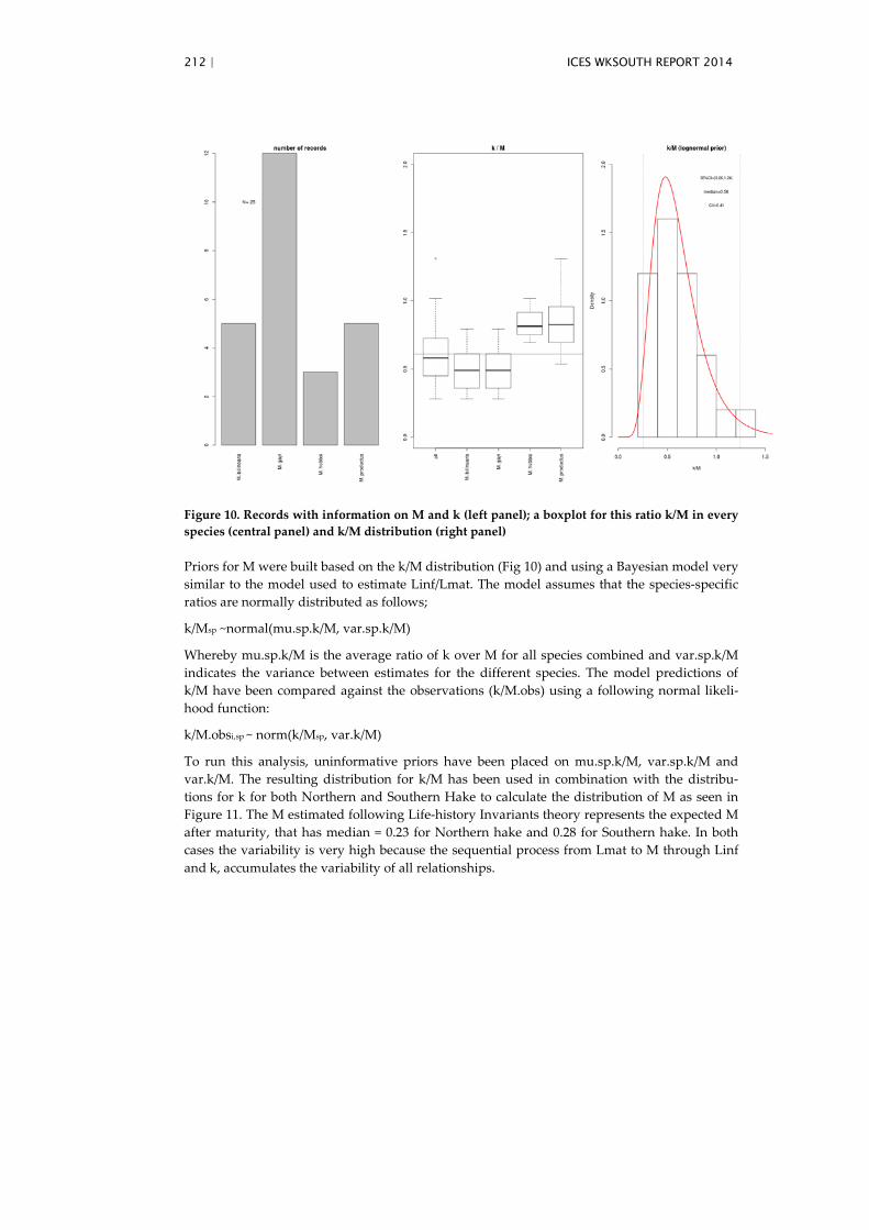
212 | ICES WKSOUTH REPORT 2014
Figure 10. Records with information on M and k (left panel); a boxplot for this ratio k/M in every species (central panel) and k/M distribution (right panel)
Priors for M were built based on the k/M distribution (Fig 10) and using a Bayesian model very similar to the model used to estimate Linf/Lmat. The model assumes that the species-specific ratios are normally distributed as follows;
k/Msp ~normal(mu.sp.k/M, var.sp.k/M)
Whereby mu.sp.k/M is the average ratio of k over M for all species combined and var.sp.k/M indicates the variance between estimates for the different species. The model predictions of k/M have been compared against the observations (k/M.obs) using a following normal likeli-hood function:
k/M.obsi,sp ~ norm(k/Msp, var.k/M)
To run this analysis, uninformative priors have been placed on mu.sp.k/M, var.sp.k/M and var.k/M. The resulting distribution for k/M has been used in combination with the distribu-tions for k for both Northern and Southern Hake to calculate the distribution of M as seen in Figure 11. The M estimated following Life-history Invariants theory represents the expected M after maturity, that has median = 0.23 for Northern hake and 0.28 for Southern hake. In both cases the variability is very high because the sequential process from Lmat to M through Linf and k, accumulates the variability of all relationships.

ICES WKSOUTH REPORT 2014 | 213
Figure 11. M prior distribution for Northern hake (left panel) and Southern hake (right panel)
Lorenzen (1996) point to the existence of an allometric relationship between natural
mortality and body weight, in fish, of the form M = a + W ^ b where is natural mortality at weight W, a is mortality at unit weight, and b is the allometric exponent. Based on empirical studies with different populations Lorenzen found out the following parameters: b=−0.288 (90% CL[−0.315, −0.261]) and a=3.00 (90% CL[2.70, 3.30]) year−1. More recently Cook (2013) uses this equation in an assessment model for haddock getting the following parameters: a=3.69 and b=-0.305 and confirming the Lorenzen assertion that b is relatively constant among different species. Figure 12 shows the M estimated for Southern hake based on Lorenzen fig-ures and hake parameters. The model produces high M at length figures for small hake (e.g. M= 1.8 for age 0 and M=3.5 for length 1cm) that decreases until 0.18 at length 130 cm or age 15.
An ulterior development of the natural mortality model will aim to the introduction of higher values for small hake based on the high predation mainly caused by cannibalism. Literature review and preliminary analysis of Southern hake will provide the information for the M for this small hake. This model will include two parameters plus the usual constant M. At this time only the prior for the constant M was estimated.

214 | ICES WKSOUTH REPORT 2014
Figure 12. Lorenzen estimates of M at length and M at age.
Table 3. Summary of the developed priors for Lmat, Linf, k and M and Linf/Lmat and k/M.
parameter function Northern Parameters Southern Parameters
L 50% maturity normal mean=42.29; sd=2.24 mean=37.95; sd=3.09
Linf (von Bertalanffy) normal mean=100.42; sd=9.48 mean=90.15; sd=10.17
k (von Bertalanffy) lognormal median=0.15; CV=0.31 median=0.17; CV=0.33
M lognormal median=0.27; CV=0.54 median=0.31; CV=0.55
Linf/Lmat normal mean=2.37; sd=0.19
k/M lognormal median=0.58; CV=0.41
GADGET runs
To analyse the sensitivity of current GADGET model to the results of the life-history invariants analysis it was decided to perform 3 runs: 1 with the medians of Linf, k and M and 2 more runs with the 25 and 75 percentiles. To be consistent with the relationship between these correlated parameters, these two runs used the following percentiles: first with 75%-Linf, 25%-k and 25%-M and second with 25% Linf, 75%-k and 75%-M. The parameters for these 3 runs are described in the following table. These parameters were set as constant and the model was fit estimating recruitment from1982 to 2012, abundance at age in 1982 (ages 1-8) and fleets selection.
Nº Run name Life-history values (constants) Lik result
1 Base (WGHMM2013) Linf = 130; k = 0.164; M=0.4 Lik= 928.26
2 LHLinf75k25M25 Linf = 110.690; k = 0.147; M=0.212 Lik= 1037.88
3 LHLinf50k50M50 Linf = 97.778; k = 0.173; M=0.279 Lik=970.76
4 LHLinf25k75M75 Linf = 87.547; k = 0.208; M=0.378 Lik=908.55

ICES WKSOUTH REPORT 2014 | 215
Compare GADGET likelihoods
Compare GADGET parameters
Compare results

216 | ICES WKSOUTH REPORT 2014
Discussion
Hake is a sex dimorphic species with different size at maturity and different growth in both sexes. Females mature larger than males and have larger sizes than males. The exercise per-formed here was done to estimate parameters for a model with sexes combined. So, the initial information for this sequential estimation was Lmat, which is the yearly L50% maturity for both sexes combined. And then, the estimated parameters for growth (k and Linf) and M cor-respond also to both sexes combined.
An assessment model like those performed for both hakes with SS3 or GADGET with sexes combined always have to make some assumptions. In this case, that Linf is equal to 130 cm and M=0.4. With these constant figures k is estimated by the model explaining the observed catch-es. The Linf estimated here showed figures around 100 cm, well below 130 cm set for ICES models. This is because Linf is estimated from a sex combined Lmat. Meanwhile in ICES Linf was mainly based on the higher observed hakes, which are females. Both approaches make different assumptions: (1) the ICES approach assumes that all hakes in the population might reach 130 cm. However we know that approximately half of the population, the males, rarely achieves 75 cm. However, since k (and also recruitment) was estimated to fit the past popula-tion productivity, it is expected that the final combination of model parameters for growth and mortality be able also to predict the future productivity. (2) On the other side, the approach presented here based on LHI would assume that all population achieves a Linf around 100 cm. In this case we lost the option of half of the population (females) growing larger and the other half growing shorter (See Cerviño, in press for comparisons among hake male and female growth and M parameters). Since fishing selection is mainly based on fish length this assump-tion might also have an impact on the productivity. Furthermore, there are a lot of catch data with figures well overestimated Linf that will be difficult to implement in the model with a short Linf. Which approach in better? ANY MODEL APPROACH BASED ON SEXES COM-BINED WILL LOST AN IMPORTANT PART OF THE REALITY. In any case 130 cm seems to be an extremely large Linf, even for females, where mean historic northern hake Lmat is about 48 cm (Dominguez et al., 2008) and the mean Linf based on LHI would be around 114 cm. An impact analysis of both approaches on assessment results and reference points may be seen on annex I.
The approach also provides information for k and M. k is conditioned to Linf so it cannot be used as a prior if Linf is different. However the prior for the correlation among k and Linf might be used if required.
M presents figures around 0.3 with a high CV (~0.5). This seems to be below current M (0.4) used in ICES models. The approach used by ICES follows the Hewitt and Hoenig (2005) ap-proach based on longevity and assuming that hake lives around 10 years. This approach pro-vides a mean M for all ages. However we have to consider that LHI approach provides M figures only for mature fish (above 40 cm aprox). M for immature fish should be estimated following other methods like Lorenzen’s (1996). These approaches might be complementary predicting that immature hake (<40 cm) M should be higher than 0.4 in order to get the mean 0.4 predicted by Hewitt and Hoenig (2005). This is in agreement with other studies based on hake that predict a high M for small hakes because of cannibalism (Jurado-Molina et al., 2006), limited food or predation, including cannibalism (Smith, 1995).
In summary, the ICES models cannot be able to estimate growth and M (apart of other parame-ters like recruitment, selection, etc), and is required to fix two of these parameters (Linf and M) allowing to estimate k. The approach presented here provide information to explore figures for this parameters that might be directly input in the model (M or Linf means); ranges to explore (e.g. inside a confident interval of 90%) or using the invariants distribution to set one of them once that other have been set.

ICES WKSOUTH REPORT 2014 | 217
References.
Beverton, R.J.H., Holt, S.J. 1959. A review of the lifespans and mortality rates of fish in nature and the relation to growth and other physiological characteristics. In: Ciba Foundation Colloquia in Ageing; The Lifespan of Animals, Churchill, London, pp. 147–77.
Beverton, R.J.H. 1992. Patterns of reproductive strategy parameters in some marine teleosts fishes. J. Fish Biol. 41: 137–160.
Cerviño, S. R. Domínguez, E. Jardim, S. Mehault, C. Piñeiro and F. Saborido-Rey. 2013. Impact of egg production and stock structure on MSY reference points. Implications for Southern hake management. Fisheries Research.138: 168-178. doi:10.1016/j.fishres.2012.07.016
Cerviño, S. In Press. Estimating growth from sex ratio-at-length data in species with sexual size dimorphism. Fisheries Research. doi:10.1016/j.fishres.2013.11.010
Cook, R.M. 2013. A fish stock assessment model using survey data when estimates of catch are unreliable. Fisheries Research, 143: 1– 11.
Charnov, E.L. 1993. Life history invariants. Some explorations of symmetry in evolutionary ecology. Oxford University Press, Oxford.
Charnov, E. and Berrigan, D. 1991. Evolution of life history patterns in animals with indeter-minate growth, particularly fish. Evol. Ecol. 5: 63-68
de Pontual, H., Groison, A. L., Piñeiro, C., and Bertignac, M. 2006. Evidence of underestimation of european hake growth in the bay of biscay, and its relationship with bias in the agreed method of age estimation. ICES Journal of Marine Science: 63(9):1674-1681.
Domínguez, R., Korta, M., Saborido-Rey, F., Murua, H., Sainza, M., Piñeiro, C., 2008. Analysis of the influence of stock structure and environmental changes in size at maturity for both European hake Atlantic populations. J. Mar. Sys. 71, 260–278.
Froese, R. and D. Pauly. Editors. 2013. FishBase. World Wide Web electronic publication. www.fishbase.org, version (04/2013).
Hewitt, D.A, and J.M. Hoenig. 2005. Comparison of two approaches to estimate natural mortal-ity based on longevity. Fish. Bull. 103: 433-437
Hilborn, R. and Liermann, M. (1998). Standing on the shoulders of giants: learning from expe-rience in fisheries. Reviews in Fish Biology and Fisheries: 8, 273-283.
Jensen, A.L., 1996. Beverton and Holt life history invariants result from optimal trade- off of reproduction and survival. Can. J. Fish. Aquat. Sci. 53, 820–822.
Jurado-Molina, J., Gatica, C. and Cubillos, L.A. 2006. Incorporating cannibalism into an age-structured model for the Chilean hake. Fisheries Research 82, 30–40
Liermann, M. and Hilborn, R. (1997). Depensation in fish stocks: a hierarchical Bayesian meta-analysis. Canadian Journal of Fisheries and Aquatic Sciences: 54, 1976-1984.
Lorenzen, K., 1996. The relationship between body weight and natural mortality in juvenile and adult fish: a comparison of natural ecosystems and aquaculture. J. Fish Biol. 49, 627–647.
Myers, R.A. and Mertz, G. (1998). Reducing the uncertainty in the biological basis of fisheries management by meta-analysis of data from many populations: a synthesis. Fisheries Re-search: 37, 51-60.
Piñeiro, C., Rey, J., de Pontual, H., and Goñi, R. 2007. Tag and recapture of European hake (Merluccius merluccius) of the northwest Iberian Peninsula: First results support fast growth hypothesis. Fisheries Research, 88:150-154
Smith, P.E. 1995. Development of the population biology of the pacific hake, Merluccius productus. CalCOFl Rep., Vol. 36

218 | ICES WKSOUTH REPORT 2014
Annex I. Comparison between Southern hake GADGET results with Linf=130 and Linf=105 cm.
Two model for Southern hake have been fit with M=0.4, k estimated and Linf set as 130 (model 1) or 105 (model 2). The quality of the fit is better for model 1 (Table 1)
Table 1. summary results
Model Linf K (estimated) Likelihood
Model 1 130 0.168 928
Model 2 105 0.189 979
Reference points
Figure 1. Yield-per-recruit (left) and absolute yield (right). Fsq is the F estimated for the last year in the model (2012). YPR and Yield are higher at all levels of F for model 1 compared to model 2. Model 1 presents a MSY a 15% higher than model 2. Fmax is quite similar in both models howev-er the stock status (current F regarding Fmax) is better for model 2

ICES WKSOUTH REPORT 2014 | 219
Figure 2. Spawning-stock biomass (left) and SPR (right) against F. SSB size at Fmax (Smsy) is a 50% higher for model 1, however the similarity in SPR for both model tell us that F SPR reference points are quite similar.
Conclusion.
Setting Linf at different values produces fits of different quality with populations of quite dif-ferent productivity (yield), different size (SSB) and different status (Fcurrent/Fref). However reference F reference points based on YPR or SPR remains relatively similar.

220 | ICES WKSOUTH REPORT 2014
WD 04 Standardization of the LPUE series of the Northern Spanish coastal bottom otter trawl fleet to tune the assessment of the Iberian megrims stocks
J. Castro, E. Abad, M. Marín, R. Morlán and A. Punzón
Instituto Español de Oceanografía (IEO): [email protected]
ABSTRACT
There are two tuning fleets which have been used in the assessment of Iberian stocks of megrim: North-ern Spanish coastal bottom otter trawlers landing in A Coruña port (“SP-CORUTR8c”) and Avilés port (“SP-AVILESTR”). However, it is known the existence of changes in the fishing strategy of this fleet in recent years, which has diversified into demersal and pelagic fishing activities. As consequence, these tuning fleets show noisy behaviour through the time-series, and they are partially used in the as-sessment of megrims (1990-1999 for “SP-CORUTR8c” tuning fleet in the assessment of four-spot me-grim and 1990-2003 for “SP-AVILESTR” in the megrim assessment). In the present work the disaggregation in métiers of the whole time-series available (1986-2012) is provided for landings and effort of the Northern Spanish coastal bottom otter trawlers landing in both harbours (A Coruña and Avilés): métier targeting demersal fish (OTB_DEF_>=55_0_0) and métier targeting a mixed of demersal and pelagic fish (OTB_MPD_>=55_0_0). The first métier is considered the most appropriate to assess benthic fish as megrims.
INTRODUCTION
Administrative control is achieved through a common fishing license for the whole Northern Spanish coastal trawl fleet, the size of which has decreased from 279 vessels in the early 1990s (STECF, 1994) to 99 vessels registered in 2012 (64.5% of reduction). During the last two dec-ades, the Northern Spanish coastal trawl fleet has been made up of boats using two main gear types, the bottom otter trawl and the bottom pair trawl. The pairtrawlers have been traditional-ly defined as a highly mono-specific fleet, targeting blue whiting (Micromesistius poutassou) and hake (Merluccius merluccius) by using a characteristic gear which permits a vertical opening up to 25 m. However, another fishing strategy targeting mackerel (Scomber scombrus) has been recently identified (Castro et al., 2010).
Regarding bottom otter trawlers, they use different type of trawl gears depending on the target species (Lema et al., 2006): traditional trawl gear to catch demersal species (“baca”) and a Verti-cal High Opening (VHO) trawl gear (“jurelera”) directed to pelagic fish. They can be alterna-tively used during the same trip, complicating the precise separation of both activities. Therefore, it was determined that the more accurate disaggregation protocol is to apply multi-variate methodologies to the landing matrix by trip and species in percentage. Punzon et al. (2010) found four different fishing strategies by using the multivariate technique CLARA (Kaufman and Rousseeuw, 1990) to a time-series of landings by trip (1983-2004): 1) trips with mixed of demersal species as hake, monkfish (Lophius piscatorius and L. budegassa), and megrim (Lepidorhombus boscii and L. whifiagonis) (each one around 10% in weight of landings), 2) trips targeting horse mackerel (Trachurus trachurus) (63%) 3) trips targeting mackerel (76%), and 4) trips targeting blue whiting (62%).
This methodology has been routinely applied to the Spanish logbooks since 2009, when the DCF regulation was implemented, in order to split the Northern Spanish coastal bottom otter trawl activity into the following two DCF métiers:
• OTB_DEF_>=55_0_0: bottom otter trawl targeting demersal species by using 70 mm mesh size (Spanish regulation: Real Decreto 1441/1999). This métier is developed by around 60 vessels (mainly between 24-40 m of length) operating in the Spanish waters of ICES Divisions VIIIc and IXa (Castro et al., 2011). In the Northern Portuguese waters of Division IXa a smaller number of vessels (around 5 vessels) develop a similar fishing strategy (Map 1). Main ports of

ICES WKSOUTH REPORT 2014 | 221
landings are in Galicia: A Coruña (30% of total ladings), Vigo (18%), Marín (13%) and Burela (11%).
• OTB_MPD_>=55_0_0: bottom otter trawl targeting a mixed of pelagic and demersal species by using 55 mm mesh size (Spanish regulation: APA/16/2002). This DCF métier cover the two fishing tactics identified by Punzon et al. (2010) targeting horse mackerel and mackerel (accompanied by some demersal species, mainly hake). This métier is developed by a large number of the same vessels developing the previous métier, but exclusively operating in Span-ish waters (mainly VIIIc). Main ports of landings are also in Galicia: A Coruña (39%), Burela (23%) and Ribeira (16%). Trips targeting mackerel show a clear seasonality concentrating in February and March.
A decline in the importance of the fourth fishing tactic targeting blue whiting started to be evi-dent from the late 1990s, probably due to competition with pair trawling (Lema et al., 2006). Since 2009, when DCF métier disaggregation started to be routinely applied to Spanish log-books, this fishing tactic never again was detected.
During the last WGHMM, a number of problems were identified in the megrims assessment in order to be analysed during the WKSOUTH benchmark (ICES, 2013). Regarding commercial data, the “SP-CORUTR8c” tuning fleet (Northern Spanish coastal bottom otter trawlers landing in A Coruña port) was partially used in the assessment of four-spot megrim (only time-series 1990-1999) due to the increasing use of the “jurelera” trawl gear targeting other species than megrim in the last decade.
Therefore, the métier disaggregation of the SP-CORUTR8c tuning fleet was developed as inter-seasonal work between WGHMM 2013 and WKSOUTH 2014. Moreover, the “SP-AVILESTR” tuning fleet (Northern Spanish coastal bottom otter trawlers landing in Avilés port), used as tuning fleet in the assessment of megrim just to 2003, was also split in DCF métiers and updat-ed (until 2012). To develop both tasks it was necessary to compile and analyse the commercial data of the period 2004-2008, which was missed between the periods available: 1983-20031 (Punzon et al., 2010) and 2009-2012 (DCF period).
1 2004 data from Punzón et al. (2010) was based in partial sampling.
MATERIAL AND METHODS
A dataset was compiled from the official logbooks of the Northern Spanish coastal bottom otter trawl fleet for the period 2004–2008, which has been facilitated by the Spanish ministry respon-sible for fisheries (MAGRAMA: “Ministerio de Agricultura, Alimentacion y Medio Ambiente”). This dataset contains information on fishing area, date of landing, landing port, base port, and landed weight of species by trip, fishing day and ICES rectangle. This dataset was used to de-velop the analytical work which is here shown.
Moreover, the original data from Punzon et al. (2010) was also available in order to split land-ings and effort by fishing tactic and port (A Coruña and Avilés) for the old time-series (1983-2003). Landings and effort data by DCF métier was also taken from the IEO databases for the recent period (2009-2012). Finally, the time-series provided to ICES (1983-2012) for the whole Northern Spanish coastal bottom otter trawl fleet was taken for raising (ICES, 2013). This last process was needed due to the low sampling level detected in some years of the old time-series (Table 1): years 1999 and 2000 in A Coruña port and years 1994-2003 for Avilés.
To classify trips, a non-hierarchical cluster technique was applied to the landings matrix by trip and species, the same methodology used by Punzón et al. (2010) and currently applied by the IEO fishery data programme. Five multivariate analyses were developed, one per year of the time-series (2004-2008). The “Clustering Large Applications” method (CLARA) is a partitioning clustering method specifically designed for clustering large datasets (Kaufman and Rousseeuw, 1990). Its algorithm works by applying a “Partitioning Around Medoids” method (PAM) to data subsets of fixed size, allowing the user to try different levels of sampling. One valuable advantage of CLARA and PAM methods is that they provide a quality index which facilitates a more objective selection of the most appropriate number of clusters. This “silhouette coefficient” is calculated for each cluster (s) and the whole clustering procedure (ASW: “average

222 | ICES WKSOUTH REPORT 2014
silhouette width”). An interpretation proposed by Kaufman and Rousseeuw (1990) identifies a reasonable structure when ASW is higher than 0.5.
Computations were performed using the R statistical language (R Development Core Team, 2008). Cluster analysis was performed using R package cluster (Maecheler et al., 2005).
RESULTS
After testing different number of groups, the highest ASW values were obtained by splitting into 4 groups for years 2004 and 2005, and by splitting into 3 clusters for years 2006-2008 (Table 2). Except for year 2004, all the ASW coefficients obtained are significant (>0.5). Table 3 shows the specific characterization for each cluster, each of them with different catch profile:
• Cluster k1: mixed landings profile where, in addition of blue whiting and horse mackerel, demersal stocks stand by their higher presence compared to the other méti-ers: anglerfish (12.5%), hake (8.7%), megrim (7%)…
• Cluster k2: the main species by weight is horse mackerel (80.4%).
• Cluster k3: the main species by weight is mackerel (83.1%).
• Cluster k4: the main species by weight is blue whiting (52.3%).
The cluster disaggregation obtained for the period analysed (2004-2008) was linked to the peri-ods 1983-2003 (Punzon et al., 2010) and 2009-2012 (DCF period): landings (t) and effort (fishing days standardized by power: fd/1000*HP/100). However, due to the low sampling level in par-ticular years of the old period, the ICES landings and effort time-series of the whole Spanish trawl activity was used in order to raise the values (Figures 1 and 2).
Due that cluster 4 has disappeared in this last decade, the first three clusters were re-aggregated into the current DCF métiers: OTB_DEF_>=55_0_0 (cluster k1 targeting demersal fish) and OTB_MPD_>=55_0_0 (integrating clusters k2 and k3 directed to horse mackerel and mackerel, respectively). Finally, as the species of megrims are not properly identified in log-books (both recorded at genus level), the ratio of species obtained by yearly sampling (IEO data) was applied to split landings by species, four-spot megrim (L. boscii) and megrim (L. whiffiagonis). Therefore, LPUE are provided by species (four-spot megrim and megrim), DCF métier (OTB_DEF_>=55_0_0 and OTB_MPD_>=55_0_0) and landing port (A Coruña and Avilés) in Tables 4-5 and Figures 3-4.
DISCUSSION
The same methodology has been applied to the three time-series available trying to establish a consistent link: 1983-2003 (obtained from Punzón et al., 2010), 2004-2008 (period recovered here) and 2009-2012 (DCF period). The results obtained show the evolution of four fishing tac-tics with different target species: demersal fish, horse mackerel, mackerel and blue whiting. This last fishing tactic shows a decreasing from the late 1990s, probably as a consequence of the increasing of the pair trawl fishing activity, which obtains higher yields per trip (Lema et al., 2006). The OTB fishing activity targeting blue whiting completely disappears in the Avilés and A Coruña fleets in 2001 and 2006, respectively.
The fishing tactic targeting horse mackerel seems to be important from the beginning of the series (Figures 1 and 2). However, it keeps being important for the A Coruña fleet while it has been practically disappeared in Avilés from the late 1990s. The other pelagic fishing tactic, the one targeting mackerel, shows lower levels of effort due to its seasonal character, mainly con-centrated in February and March. It takes advantage of the spawning migration of mackerel to the north coast of Spain at the beginning of the year (Sola et al., 1990), as do other fleets target-ing mackerel in the same areas, such as purse-seiners (Villamor et al., 1997) and handlines (Punzón and Villamor, 2009). However, an increase, more evident in Avilés, can be observed from 2000, probably in response to improved market conditions for mackerel (Punzón et al., 2004). The fishing tactic targeting demersal fish shows a moderate decreasing through the time-series, and results the more important fishing tactic in Avilés compared with the re-mained trawl fishing tactics.

ICES WKSOUTH REPORT 2014 | 223
Since 2009, these three fishing tactics are re-aggregated in two DCF métiers following the pan-European “Data Collection Framework” for fishery data: OTB_DEF_>=55_0_0 (corresponds to fishing tactic targeting demersal fish) and OTB_MPD_>=55_0_0 (integrates both fishing tactics targeting horse mackerel and mackerel). This procedure was applied backwards to the recov-ered time-series in order to obtain a robust index (LPUE) feasible to be used as tuning fleet. Due to benthic species are target objective of OTB_DEF_>=55_0_0, it is recommended to use the LPUE of this métier as tuning fleet in the assessment of megrims.
LPUE of A Coruña OTB_DEF_>=55_0_0 shows different levels and trends between megrim species, being higher (average of 13.7 and 2.4 t by standardize effort unit for four-spot megrim and megrim, respectively) and with a remarkable increasing trend for four-spot megrim since middle 90’s (Figure 3). However, Avilés OTB_DEF_>=55_0_0 gives similar indices (13.7 and 13.8 t by standardize effort unit for four-spot megrim and megrim, respectively), showing a more balanced abundance of both species in Cantabrian waters than was observed in North-western Iberian waters (Figure 4).
The changes detected in the fishing strategy of a fleet may have led to variations in trends of the tuning indices used in stock assessment which are not related to species abundance. There-fore, LPUE series should be computed by métier in order to provide more homogeneous yield-ing indices which can improve the knowledge of the stock evolution.
CONCLUSIONS
Eight new LPUE time-series can be obtained by DCF métier, landing port and megrim stock. However, the four time-series of the métier targeting demersal fish are recommended to be tested in the assessment of megrims:
• LPUE of métier OTB_DEF_>=55_0_0 in A Coruña port for four-spot megrim (LDB).
• LPUE of métier OTB_DEF_>=55_0_0 in A Coruña port for megrim (MEG).
• LPUE of métier OTB_DEF_>=55_0_0 in Avilés port for four-spot megrim (LDB).
• LPUE of métier OTB_DEF_>=55_0_0 in Avilés port for megrim (MEG).
References
Castro, J., Punzón, A., Pierce, G.J., Marín, M. & Abad, E. 2010. Identification of métiers of the Northern Spanish coastal bottom pair trawl fleet by using the partitioning method CLARA. Fisheries Research 102: 184-190.
Castro, J., Marín, M. and Vázquez, A. 2011. Fichas descriptivas de los métier DCF de zona IC-ES. Proyecto SAP_ATLAN, Programa Pesca ICES. Instituto Español de Oceanografía. 64 pp.
ICES. 2013. Report of the Working Group on the Assessment of Southern Shelf Stocks of Hake, Monk and Megrim (WGHMM), 10 - 16 May 2013, ICES Headquarters, Copenhagen. ICES CM 2013/ACOM:11A. 719 pp.
Kaufman, L. and Rousseeuw, P.J., 1990. Finding Groups in Data: An Introduction to Cluster Analy-sis. John Wiley & Sons, Inc., New York.
Lema, L., Pérez, N. and Araujo, H. 2006. Discards of Spanish trawler fleets operating in the Bay of Biscay in 2000. Scientia Marina, 70: 173–181
Maecheler, M., Rousseeuw, P., Struyf, A., Hubert, M., 2005. Cluster Analysis Basics and Exten-sions. R Package, http://www.r-project.org.
Punzón, A., and Villamor, B. 2009. Does the timing of the spawning migration change for the southern component of the North East Atlantic Mackerel (Scomber scombrus, L. 1758)? An approximation using fishery analyses. Continental Shelf Research, 29: 1195–1204.

224 | ICES WKSOUTH REPORT 2014
Punzón, A., Villamor, B., and Preciado, I. 2004. Analisys of the handline fishery targeting mackerel (Scomber scombrus, L.) in the North of Spain (ICES Division VIIIbc). Fisheries Re-search, 69: 189–204.
Punzón, A., Hernández, C., Abad, E., Castro, J., Pérez, N., and Trujillo, V. 2010. Spanish otter trawl fisheries in the Cantabrian Sea. ICES Journal of Marine Science 67: 1604–1616.
R Development Core Team, 2008. R: A Language and Environment for Statistical Computing. R Foundation for Statistical Computing, Vienna, Austria, ISBN 3-900051-07-0, URL http://www.r-project.org.
Sola, A., Motos, L., Franco, C., and Lago de Lanzos, A. 1990. Seasonal occurrence of pelagic fish eggs and larvae in the Cantabrian Sea (VIIIc) and Galicia (IXa) from 1987 to 1989. ICES Document CM 1990/H: 26.
Villamor, B., Abaunza, P., Lucio, P., and Porteiro, C. 1997. Distribution and age structure of mackerel (Scomber scombrus, L.) and horse mackerel (Trachurus trachurus, L.) in the north coast of Spain, 1989–1994. Scientia Marina, 61: 345–366.
Table 1. Available databases of the Northern Spanish coastal bottom otter trawl fleet used in the time-series compilation: number of trips by year and port (A Coruña and Avilés). [Numbers be-tween brackets are based in partial samplings; “na”: not available].
A Coruña Avilés
Year Punzón et al (2010)
LOGBOOKS Punzón et al (2010)
LOGBOOKS
1983 na na 2698 na
1984 na na 2331 na
1985 na na 2195 na
1986 4446 na 2390 na
1987 4010 na 1858 na
1988 4873 na 2069 na
1989 5295 na na na
1990 5542 na 1992 na
1991 5089 na 1786 na
1992 5055 na 1107 na
1993 5694 na 1070 na
1994 5169 na na na
1995 5470 na [144] na
1996 4858 na na na
1997 4789 na na na
1998 3494 na [110] na
1999 [263] na [427] na
2000 [504] na [378] na
2001 3532 na [246] na
2002 3211 na [314] na
2003 2690 na [269] na
2004 [489] 3351 [374] 538
2005 na 3542 na 855
2006 na 3326 na 881
2007 na 3412 na 631

ICES WKSOUTH REPORT 2014 | 225
2008 na 3216 na 579
2009 na 3161 na 666
2010 na 3054 na 527
2011 na 2312 na 488
2012 na 2366 na 680
Table 2. Results of CLARA clustering (k: number of clusters; ASW: average silhouette width; and s: silhouette coefficient by cluster).
Year k ASW S(k1) S(K2) S(K3) S(k4)
2004 4 0.45 0.05 0.68 0.59 0.47
2005 4 0.50 0.22 0.71 0.75 0.36
2006 3 0.56 0.25 0.69 0.77 --
2007 3 0.58 0.36 0.74 0.70 --
2008 3 0.54 0.40 0.70 0.73 --
Table 3. Mean landing profile (%) by cluster (mean of the analysed period 2004-2008).
SPECIES AL3 K1 K2 K3 K4
Atherinidae SIL 0.3 0 0 0
Boops boops BOG 0.4 0.3 0 0.1
Eledone spp OCM 4.0 0.2 0.2 0.5
Galeorhinus galeus GAG 0.4 0 0 0
Galeus melastomus SHO 0.4 0 0 0
Illex illecebrosus SQI 2.4 0.1 0 0.9
Lepidorhombus spp LEZ 7.0 1.0 0.2 4.4
Loligo spp SQC 1.3 0.2 0 1.4
Lophiidae ANF 12.5 1.4 0.4 5.6
Merluccius merluccius HKE 8.7 2.4 0.7 5.2
Micromesistius poutassou WHB 24.7 1.8 0.7 52.3
Mullus spp MUX 0.6 0 0 0
Nephrops norvegicus NEP 1.0 0 0 0.5
Octopus vulgaris OCC 1.8 0.1 0.1 0.4
OTHERS OTH 8.5 2 4.6 4.3
Pagellus acarne SBA 0.3 0.1 0 0.2
Phycis blennoides GFB 0.3 0 0 0
Raja spp SKA 1.5 0.4 0.1 0.4
Scomber scombrus MAC 8.0 8.8 83.1 5.4
Scyliorhinidae SYX 0.4 0 0 0
Trachurus spp JAX 10.8 80.4 9.5 17.3
Triglidae GUX 1.3 0.1 0.1 0.4
Trisopterus luscus BIB 3.9 0.5 0.2 0.7

226 | ICES WKSOUTH REPORT 2014
Table 4. LPUE (t/fd/1000*HP/100) of four-spot megrim (L. boscii) by DCF métier (OTB_DEF_>=55_0_0 and OTB_MPD_>=55_0_0) and port (A Coruña and Avilés).
A Coruña Avilés
Year OTB_DEF_>-55_0_0 OTB_MPD_>-55_0_0 OTB_DEF_>-55_0_0 OTB_MPD_>-55_0_0
1986 9.8 8.8 6.8 4.5
1987 14.9 11.7 10.4 8.2
1988 7.0 6.3 14.0 12.5
1989 6.2 4.1 10.9 9.3
1990 7.8 4.2 19.7 17.6
1991 9.8 4.2 12.2 10.1
1992 6.6 3.5 15.5 12.5
1993 7.8 4.2 16.1 13.0
1994 10.6 6.6 14.0 11.0
1995 11.0 7.6 24.7 15.3
1996 7.2 6.2 16.4 12.4
1997 7.9 5.4 18.7 13.9
1998 14.4 11.6 11.0 13.3
1999 11.7 13.2 11.3 9.7
2000 16.4 12.7 13.8 10.1
2001 20.2 9.8 12.5 9.6
2002 13.0 8.0 11.3 4.6
2003 11.6 5.7 5.7 1.9
2004 18.2 8.7 14.8 5.0

ICES WKSOUTH REPORT 2014 | 227
2005 13.6 6.0 15.2 1.9
2006 15.9 6.5 11.6 1.5
2007 17.9 7.3 8.9 1.8
2008 22.0 8.1 7.2 0.6
2009 17.3 6.9 18.5 2.2
2010 29.3 13.3 25.4 3.1
2011 24.8 11.9 19.6 4.2
2012 16.7 10.1 4.3 0.8
AVERAGE 13.7 7.9 13.7 7.8
Table 5. LPUE (t/fd/1000*HP/100) of megrim (L. whiffiagonis) by DCF métier (OTB_DEF_>=55_0_0 and OTB_MPD_>=55_0_0) and port (A Coruña and Avilés).
A Coruña Avilés
Year OTB_DEF_>-55_0_0 OTB_MPD_>-55_0_0 OTB_DEF_>-55_0_0 OTB_MPD_>-55_0_0
1986 2.2 2.0 21.2 14.2
1987 2.9 2.2 17.6 13.9
1988 2.6 2.3 24.6 22.0
1989 2.0 1.4 19.8 16.9
1990 3.1 1.7 36.9 32.9
1991 3.1 1.3 15.0 12.4
1992 3.1 1.6 15.5 12.5
1993 1.5 0.8 18.5 15.0
1994 3.8 2.3 11.4 8.9
1995 0.9 0.6 9.7 6.0

228 | ICES WKSOUTH REPORT 2014
1996 2.4 2.1 17.1 13.0
1997 2.4 1.6 19.2 14.2
1998 3.6 2.9 12.2 14.7
1999 2.6 3.0 12.7 10.9
2000 3.3 2.6 10.5 7.6
2001 2.3 1.1 11.2 8.5
2002 2.0 1.2 9.1 3.7
2003 1.7 0.8 5.7 1.9
2004 1.7 0.8 14.8 5.0
2005 1.3 0.6 11.1 1.4
2006 1.4 0.6 9.6 1.2
2007 1.8 0.7 4.8 1.0
2008 1.3 0.5 5.3 0.4
2009 1.1 0.4 5.1 0.6
2010 2.0 0.9 11.7 1.4
2011 3.4 1.6 18.7 4.0
2012 5.6 3.5 4.4 0.8
AVERAGE 2.4 1.5 13.8 9.1

ICES WKSOUTH REPORT 2014 | 229

230 | ICES WKSOUTH REPORT 2014

ICES WKSOUTH REPORT 2014 | 231

232 | ICES WKSOUTH REPORT 2014
Annex 3: Participants list
Data Compilation Workshop on Southern Megrim and Hake Stocks (DCWKSOUTH)
30 October–1 November 2013
LIST OF PARTICIPANTS Name Address Phone/Fax E-mail
Esther Abad Instituto Español de Oceanografía. Centro Oceanográfico de Vigo
P.O. Box 1552
E-36200 Vigo (Pontevedra)
Spain
Phone +34 986 492 111
Fax +34 986 498 626
Finlay Burns (by WebEx)
Marine Scotland Science Marine Laboratory 375 Victoria Road PO Box 101 Aberdeen AB11 9DB UK
+44 1224876544 +44 1224295376
José Castro Pampillón
Instituto Español de Oceanografía (IEO) P.O. Box 1552 E-36200 Vigo (Pontevedra) Spain
Phone +34 986 49 2111 Fax +34 986 49 8626
Santiago Cerviño
Instituto Español de Oceanografía Centro Oceanográfico de Vigo P.O. Box 1552 E-36200 Vigo (Pontevedra) Spain
Phone +34 986492111 Fax +34 986498626
Anne Cooper (ICES secretariate)
Professional Office for Advisory Services International Council for the Exploration of the Sea (ICES) H.C. Andersens Boulevard 44-46 1553 Copenhagen V. Denmark.
Phone +44 3338 6767
Joao Figueiredo Pereira (by correspondance)
Portuguese Institute for the Sea and the Atmosphere (IPMA) Avenida de Brasilia 1449-006 Lisbon Portugal
Phone +351 213027044 Fax +351 213015948

ICES WKSOUTH REPORT 2014 | 233
Name Address Phone/Fax E-mail
Dorleta Garcia AZTI-Tecnalia Sukarrieta Txatxarramendi ugartea z/g E-48395 Sukarrieta (Bizkaia) Spain
Phone +34 946 574 000 Fax +34 946 870 006
Baltasar Patino Instituto Español de Oceanografía (IEO) P.O. Box 1552 E-36200 Vigo (Pontevedra) Spain
Nelida Perez Instituto Español de Oceanografía (IEO) P.O. Box 1552 E-36200 Vigo (Pontevedra) Spain
Lisa Readdy (ICES Chair)
Centre for Environment, Fisheries and Aquaculture Science (Cefas) Lowestoft Laboratory Pakefield Road NR33 0HT Lowestoft Suffolk UK
Phone +44 1502 52 4319 Fax +44 1502 52 4511
Francisco Velasco (by WebEx)
Instituto Español de Oceanografía Centro Oceanográfico de Santander Promontorio de San Martin s/n PO Box 240 39080 Santander Spain
+34 942 291060 +34 942 275072
Benchmark Workshop on Southern Megrim and Hake Stocks (WKSOUTH)
3 February–7 February 2014
LIST OF PARTICIPANTS

234 | ICES WKSOUTH REPORT 2014
Name Address Phone/Fax E-mail
Esther Abad Instituto Español de Oceanografía. Centro Oceanográfico de Vigo
P.O. Box 1552
E-36200 Vigo (Pontevedra)
Spain
Phone +34 986 492 111
Fax +34 986 498 626
Ricardo Alpoim (by correspondance)
IPMA Avenida de Brasilia PT-1449-006 Lisbon Portugal
Phone +351 21 302 7024 Fax +351 21 301 5948
Alexandre Aires-da-Silva (External expert)
Inter-American Tropical Tuna Commission 8901 La Jolla Shores Drive La Jolla CA 92037-1508 USA
Phone +1 858 546 7100 Fax + 1 858 546 7133
Michel Bertignac
IFREMER Brest Laboratoire LBH BP 70 F-29280 Plouzané France
Phone +33 298 224 525 Fax +33 298 224 653
José Castro Instituto Español de Oceanografía (IEO) P.O. Box 1552 E-36200 Vigo (Pontevedra) Spain
Phone +34 986 49 2111 Fax +34 986 49 8626
Santiago Cervino
IFREMER Brest Laboratoire LBH BP 70 F-29280 Plouzané France
Phone +33 298 224 525 Fax +33 298 224 653
Anne Cooper (ICES secretariat)
Professional Office for Advisory Services International Council for the Exploration of the Sea (ICES) H.C. Andersens Boulevard 44-46 1553 Copenhagen V. Denmark.
Phone +44 3338 6767
Chris Darby (by WebEx)
Centre for Environment, Fisheries and Aquaculture Science (Cefas) Lowestoft Laboratory Pakefield Road NR33 0HT Lowestoft Suffolk UK
Phone +44 1502 52 4329 Fax +44 1502 52 4511

ICES WKSOUTH REPORT 2014 | 235
Name Address Phone/Fax E-mail
Enrique De Cardenas Gonzalez
Carmen Fernandez
Joao Figueiredo Pereira
Portuguese Institute for the Sea and the Atmosphere (IPMA) Avenida de Brasilia 1449-006 Lisbon Portugal
Phone +351 213027044 Fax +351 213015948
Dorleta Garcia AZTI-Tecnalia Sukarrieta Txatxarramendi ugartea z/g E-48395 Sukarrieta (Bizkaia) Spain
Phone +34 946 574 000 Fax +34 946 870 006
Daniel Howell (External expert)
Catherine Michielsens (External Chair)
Pacific Salmon Commission 600-1155 Robson street Vancouver, BC Canada V6E 1B5
Phone +1 604 684 8081 Fax +1 604 666 8707
Lisa Readdy (ICES Chair)
Centre for Environment, Fisheries and Aquaculture Science (Cefas) Lowestoft Laboratory Pakefield Road NR33 0HT Lowestoft Suffolk UK
Phone +44 1502 52 4319 Fax +44 1502 52 4511

236 | ICES WKSOUTH REPORT 2014
Annex 4: WKSOUTH review of biological reference point for Southern and Northern hake.
Participants: Catherine Michielsens (External Chair), Lisa Readdy (Chair), Carmen Fernandez, Daniel Howell, Santiago Cervino, Esther Abad, Joao Figueiredo Pereira, Anne Cooper (ICES secretariat).
WKSOUTH members met, via WebEx, to discuss proposed biological reference points for two stocks of hake put forward by the expert working group for the Bay of Biscay and Iberic Wa-ters Ecoregion (WGBIE)
Hake in Divisions VIIIc and IXa (Southern stock) During the expert working group meeting, WGBIE in 2014, it was discussed that the Blim value originally set (35 000 tonnes) should no longer be considered an appropriate recovery target, due to the fact that this estimate was based on an earlier stock assessment model, whereas the current assessment model indicates that 35 000 tonnes is no longer in the range of historic SSBs produced by the model. Therefore, Blim would need updating, taking into account the current stock assessment. WKSOUTH members agreed with this conclusion.
The diagnostics from stock recruit relationship showed no real trend in recruitment within the range of historically observed SSBs. WKSOUTH agreed that the justification used by the expert working group, WGBIE, for selecting the new proposed Blim value was appropriate.
WKSOUTH also agreed that because the lowest SSB showed (slightly) below average recruit-ment, it would be more appropriate and more precautionary to select the lowest SSB which produced average or above average recruitment. This leads to choosing Blim close to the 5th lowest value in the historical series
WKSOUTH recommended that WGBIE should also consider a Bpa and an MSY Btrigger for this stock in the near future.
Hake in Divisions IIIa, Subareas IV, VI and VII and Divisions VIIIa,b,d (Northern stock)
Using the new accepted benchmarked assessment, WGBIE produced the following new refer-ence points: Blim, Bpa, MSY Btrigger and Fmsy.
As with Southern hake, Blim for Northern hake was selected based on the Bloss approach due to the fact that the Hockey Stick relationship produced a potential Blim (at the breakpoint of the hockey-stick) which was higher than a large number of the historical SSB values. Considering that the stock has shown considerable increases in SSB from low SSB levels, even under fishing mortalities substantially above the Fmsy value proposed by WGBIE, while taking into account a more precautionary approach (hence, avoiding to choose Bloss as Blim), WKSOUTH agreed with WGBIE that the SSB in 2006, 25% higher than the lowest observed SSB, was an appropri-ate value to use given the justification outlined in Annex R of the WGBIE 2014 report.
WKSOUTH agreed with the application of the default approach (used by many ICES stocks) to produce Bpa and MSY Btrigger to the northern hake stock.
WKSOUTH agreed that the methodology used to derive Fmsy and to evaluate the ICES MSY harvest control rule followed the guidelines set out by ICES within the expert workshop WKMSYREF2 (ICES 2014/ACOM:47). Because of the features of the northern hake assessment, the software put forward by WKMSYREF2 (PlotMSY and EqSim) could not be applied to northern hake. It was noted that the R program developed specifically for northern hake is similar to the software available (in particular, EqSim), but takes into account the differing data structure of the Hake model. Having viewed all the available diagnostics from the northern hake results and considering the consistency between the methods, WKSOUTH were happy with the outcomes from this software and accepted all the biological reference point proposed by WGBIE for this stock.

ICES WKSOUTH REPORT 2014 | 237
References ICES. 2014. Report of the Workshop to consider reference points for all stocks(WKMSYREF2),
8-10 January 2014, ICES Headquarters, Copenhagen, Denmark. ICES CM 2014/ACOM:47. 91 pp.
Related Documents