® The contents of this report reflect the views of the authors, who are responsible for the facts and the accuracy of the information presented herein. This document is disseminated under the sponsorship of the Department of Transportation University Transportation Centers Program, in the interest of information exchange. The U.S. Government assumes no liability for the contents or use thereof. IntelliDrive Technology based Yellow Onset Decision Assistance System for Trucks Report # MATC-UNL: 421 Final Report Anuj Sharma, Ph.D. Assistant Professor Department of Civil, Environmental, and Architectural Engineering University of Nebraska-Lincoln Nathaniel Burnett Graduate Research Assistant Sepideh S. Aria Graduate Research Assistant 2012 A Cooperative Research Project sponsored by the U.S. Department of Transportation Research and Innovative Technology Administration 25-1121-0001-421

Welcome message from author
This document is posted to help you gain knowledge. Please leave a comment to let me know what you think about it! Share it to your friends and learn new things together.
Transcript
®
The contents of this report reflect the views of the authors, who are responsible for the facts and the accuracy of the information presented herein. This document is disseminated under the sponsorship of the Department of Transportation
University Transportation Centers Program, in the interest of information exchange. The U.S. Government assumes no liability for the contents or use thereof.
IntelliDrive Technology based Yellow Onset Decision Assistance System for Trucks
Report # MATC-UNL: 421 Final Report
Anuj Sharma, Ph.D.Assistant ProfessorDepartment of Civil, Environmental, and Architectural EngineeringUniversity of Nebraska-Lincoln
Nathaniel BurnettGraduate Research AssistantSepideh S. Aria Graduate Research Assistant
2012
A Cooperative Research Project sponsored by the U.S. Department of Transportation Research and Innovative Technology Administration
25-1121-0001-421
IntelliDrive Technology based Yellow Onset Decision Assistance System for Trucks
Anuj Sharma, Ph.D.
Assistant Professor
Department of Civil, Environmental, and Architectural Engineering
University of Nebraska–Lincoln
Nathaniel Burnett
Graduate Research Assistant
Department of Civil, Environmental, and Architectural Engineering
University of Nebraska–Lincoln
Sepideh S. Aria
Graduate Research Assistant
Department of Civil, Environmental, and Architectural Engineering
University of Nebraska–Lincoln
A Report on Research Sponsored by
Mid-America Transportation Center
University of Nebraska-Lincoln
July 2012
ii
Technical Report Documentation Page
1. Report No.
25-1121-0001-421
2. Government Accession No.
3. Recipient's Catalog No.
4. Title and Subtitle
IntelliDrive Technology based Yellow Onset Decision Assistance System for
Trucks
5. Report Date
July 2012
6. Performing Organization Code
7. Author(s)
Anuj Sharma, Nathaniel Burnett, and Sepideh S. Aria
8. Performing Organization Report No.
25-1121-0001-421
9. Performing Organization Name and Address
Mid-America Transportation Center
2200 Vine St.
PO Box 830851
Lincoln, NE 68583-0851
10. Work Unit No. (TRAIS)
11. Contract or Grant No.
12. Sponsoring Agency Name and Address
Research and Innovative Technology Administration
1200 New Jersey Ave., SE
Washington, D.C. 20590
13. Type of Report and Period
Covered
August 2010-June 2012
14. Sponsoring Agency Code
MATC TRB RiP No. 28683
15. Supplementary Notes
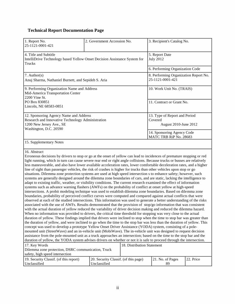
16. Abstract
Erroneous decisions by drivers to stop or go at the onset of yellow can lead to incidences of premature stopping or red
light running, which in turn can cause severe rear end or right angle collisions. Because trucks or busses are relatively
less maneuverable, and also have lower available acceleration rates, lower comfortable deceleration rates, and a higher
line of sight than passenger vehicles, the risk of crashes is higher for trucks than other vehicles upon stop or go
situations. Dilemma zone protection systems are used at high speed intersection s to enhance safety; however, such
systems are generally designed around the dilemma zone boundaries of cars, and are static, lacking the intelligence to
adapt to existing traffic, weather, or visibility conditions. The current research examined the effect of information
systems such as advance warning flashers (AWFs) on the probability of conflict at onset yellow at high-speed
intersections. A probit modeling technique was used to establish dilemma zone boundaries. Based on dilemma zone
boundaries, probability of perceived conflict curves were computed and compared against actual conflicts that were
observed at each of the studied intersections. This information was used to generate a better understanding of the risks
associated with the use of AWFs. Results demonstrated that the provision of stop/go information that was consistent
with the actual duration of yellow reduced the variability of driver decision making and reduced the dilemma hazard.
When no information was provided to drivers, the critical time threshold for stopping was very close to the actual
duration of yellow. These findings implied that drivers were inclined to stop when the time to stop bar was greater than
the duration of yellow, and were inclined to go when the time to the stop bar was less than the duration of yellow. This
concept was used to develop a prototype Yellow Onset Driver Assistance (YODA) system, consisting of a pole-
mounted unit (StreetWave) and an in-vehicle unit (MobiWave). The in-vehicle unit was designed to request decision
assistance from the pole-mounted unit as a truck approaches an intersection; based on the time to the stop bar and the
duration of yellow, the YODA system advises drivers on whether or not it is safe to proceed through the intersection.
17. Key Words
Dilemma zone protection, DSRC communication, Truck
safety, high speed intersection
18. Distribution Statement
19. Security Classif. (of this report)
Unclassified
20. Security Classif. (of this page)
Unclassified
21. No. of Pages
89
22. Price
iii
Table of Contents
Acknowledgments viii
Disclaimer ix
Abstract x
Chapter 1Introduction and Objectives 1
Chapter 2 Literature Review 7
2.1 Introduction 7
2.2 Dilemma Zone Definitions 7
2.2.1 Type I Dilemma Zone 7
2.2.2 Type II Dilemma Zone (Indecision Zone or Option Zone) 12
2.3 Effects of Yellow Length on Driver Behavior 17
2.4 Mitigation of Dilemma Zones 18
2.4.1 Green Extension 18
2.4.2 Green Termination 18
2.4.3 D-CS 19
2.4.4 SOS – Self Optimizing Signal Control 20
2.4.5 Wavetronix SmartSensor Advance 20
2.4.6 Advance Warning 21
2.4.6.1 Advanced warning’s effects on RLR 21
2.5 Traffic Conflicts 23
2.5.1 Traffic Conflict Technique 25
2.5.2 Traffic Conflicts at the Onset of Yellow 26
2.6 Dilemma Zone Hazard Models 27
2.7 Summary 29
Chapter 3 Data Collection 30
3.1 Introduction 30
3.2 Data Collection Sites 30
3.2.1 US 77 and Saltillo Rd. 30
3.2.2 Highway 2 and 84th St. 30
3.2.3 US 77 and Pioneers 31
3.2.4 Highway 34 and N79 31
3.2.5 Highway 75 and Platteview Rd. 32
3.2.6 SR32 and SR 37 32
3.3 Data Collection 34
3.3.1 Data Collection Setup 35
3.4 Validation 39
3.5 Mobile Trailer Data Collection Setup 40
3.5.1 Mobile Trailer Validation 45
3.6 Noblesville Site Data Collection Setup 46
3.6.1 Noblesville Site Validation 47
3.7 Data Reduction 48
3.8 Summary 51
Chapter 4 Role of Information on Dilemma Hazard Function 52
4.1Theory underlying driver decision making 52
4.2Traffic Conflicts 55
iv
4.3 The Effect of Information 56
4.4 Data Analysis and Results 58
4.4.1 Best Fit Model Parameters 58
4.4.2 Dilemma Zone Boundaries and Effect on Stopping 59
4.5 Discussion 63
4.6 Conclusions 66
Chapter 5 Development of the YODA System Prototype 67
5.1 Introduction 67
5.2 Prototype Assembly 68
5.3 File System 76
5.3.1General.c and General.h. 77
5.3.2 UDP.c and UDP.h 77
5.3.3 Car.c 77
5.3.4 Station.c 78
5.3.5 Its_Trafficlight.c 78
5.4 Wireless Communication 79
Chapter 6 Summary and Conclusions 81
6.1 Future Research 82
References 83
v
List of Figures
Figure 2.1 Illustration of Type I dilemma zone 8
Figure 2.2 Previously reported perception reaction times 11
Figure 2.3 Illustration of Type II dilemma zone 12
Figure 2.4 Dilemma zone boundaries (50 mph) 16
Figure 2.5 Comparison of traditional and proposed surrogate methods of safety 24
Figure 3.1View of advance warning flashers prior to intersection 31
Figure 3.2 Aerial views of data collection sites 33
Figure 3.3 Schematic of data collection at Highway 2 and 84th St. 36
Figure 3.4 Visualization of Wavetronix SmartSensor Advance 37
Figure 3.5 Visualization of Wavetronix SmartSensor HD 37
Figure 3.6 Visualization of Axis 232D+ dome camera 38
Figure 3.7 Display of recorded vehicular movement through data collection site 38
Figure 3.8 MTi-G Setup (85) 39
Figure 3.9 Example comparison between WAD and Xsens 40
Figure 3.10 Mobile data collection trailer 41
Figure 3.11 Safe Track portable signal phase reader 42
Figure 3.12 Portable sensor pole cabinet 43
Figure 3.13 Mobotix Q24M camera 44
Figure 3.14 Mobile trailer data collection environment 45
Figure 3.15 Example comparison between WAD, GPS, & Xsens 46
Figure 3.16 Data collection environment at Noblesville, IN 47
Figure 3.17 Example comparison between WAD and GPS (86) 48
Figure 3.18 Sample data reduction form 49
Figure 3.19 Example of linear fit to vehicle 50
Figure 3.20 Example of two-degree polynomial fit to vehicle 50
Figure 4.1 Critical distances along probability of stopping curve 55
Figure 4.2 Effect of information provided to drivers 57
Figure 4.3 Probability of stopping curves 60
Figure 4.4 Probability of severe conflicts at different sites 61
Figure 4.5 Calculated weighted risks 62
Figure 4.6 Proportion of vehicles performing sever deceleration or RLR 63
Figure 4.7 Hypothetical probability of stopping curves 64
Figure 4.8 Comparison between actual and perceived yellow lengths 65
Figure 5.1 Savari network (Savarinetworks 2012) devices, StreetWave on left
and MobiWave on right 67
vi
List of Tables
Table 2.1 Variability in previously reported deceleration rates 11
Table 3.1 Detailed site characteristics 32
Table 3.2 Summary of data collected at AWF locations 34
Table 3.3 Summary of data collection at Noblesville 35
Table 4.1 Probit model results 59
vii
List of Abbreviations
Mid-America Transportation Center (MATC)
Level of Service (LOS)
Advance Warning Flasher (AWF)
Wide Area Detector (WAD)
Intelligent Transportation System (ITS)
Coordinated Universal Time (UTC)
Greenwich Mean Time (GMT)
viii
Acknowledgments
The research team would like to thank the Nebraska Department of Roads (especially
Kent Wohlers, Bob Malquist, and Matt Neeman) and the City of Lincoln Public Works
Department (especially Josh Meyers and Larry Jochum). We are grateful to Brad Giles from
Wavetronix, who guided the setup of the detector data acquisition at the test sites and helped to
generate custom codes for data collection. Thanks also go to the business team of the Mid-
America Transportation Center (MATC), who contributed to this research by arranging
transportation and providing technical support.
ix
Disclaimer
The contents of this report reflect the views of the authors, who are responsible for the
facts and the accuracy of the information presented herein. This document is disseminated under
the sponsorship of the U.S. Department of Transportation’s University Transportation Centers
Program, in the interest of information exchange. The U.S. Government assumes no liability for
the contents or use thereof.
x
Abstract
Erroneous decisions by drivers to stop or go at the onset of yellow can lead to incidences
of premature stopping or red light running, which in turn can cause severe rear end or right angle
collisions. Because trucks or busses are relatively less maneuverable, have lower available
acceleration and lower comfortable deceleration rates, and have a higher line of sight than do
passenger vehicles, the risk of crashes is higher for trucks than other vehicles upon stop or go
situations. Dilemma zone protection systems are used at high speed intersection s to enhance
safety; however, such systems are generally designed around the dilemma zone boundaries of
cars, and are static, lacking the intelligence to adapt to existing traffic, weather, or visibility
conditions. The current research examined the effect of information systems such as advance
warning flashers (AWFs) on the probability of conflict at onset yellow at high-speed
intersections. A probit modeling technique was used to establish dilemma zone boundaries.
Based on dilemma zone boundaries, probability of perceived conflict curves were computed and
compared against actual conflicts that were observed at each of the studied intersections. This
information was used to generate a better understanding of the risks associated with the use of
AWFs. Results demonstrated that the provision of stop/go information that was consistent with
the actual duration of yellow reduced the variability of driver decision making and reduced the
dilemma hazard. When no information was provided to drivers, the critical time threshold for
stopping was very close to the actual duration of yellow. These findings implied that drivers
were inclined to stop when the time to stop bar was greater than the duration of yellow, and were
inclined to go when the time to the stop bar was less than the duration of yellow. This concept
was used to develop a prototype Yellow Onset Driver Assistance (YODA) system, consisting of
a pole-mounted unit (StreetWave) and an in-vehicle unit (MobiWave). The in-vehicle unit was

xi
designed to request decision assistance from the pole-mounted unit as a truck approaches an
intersection; based on the time to the stop bar and the duration of yellow, the YODA system
advises drivers on whether or not it is safe to proceed through the intersection.
1
Chapter 1Introduction and Objectives
According to the National Highway Traffic Safety Administration (NHTSA), the total
cost of motor vehicle collisions in the United States in 2006 was estimated at $230.6 billion
(National Highway Traffic Safety Administration 2007). The total cost of motor vehicle
collisions in the State of Nebraska was projected at $2.3 billion in 2007 (State of Nebraska
2007). Intersection or intersection-related crashes accounted for nearly 40.5% of all reported
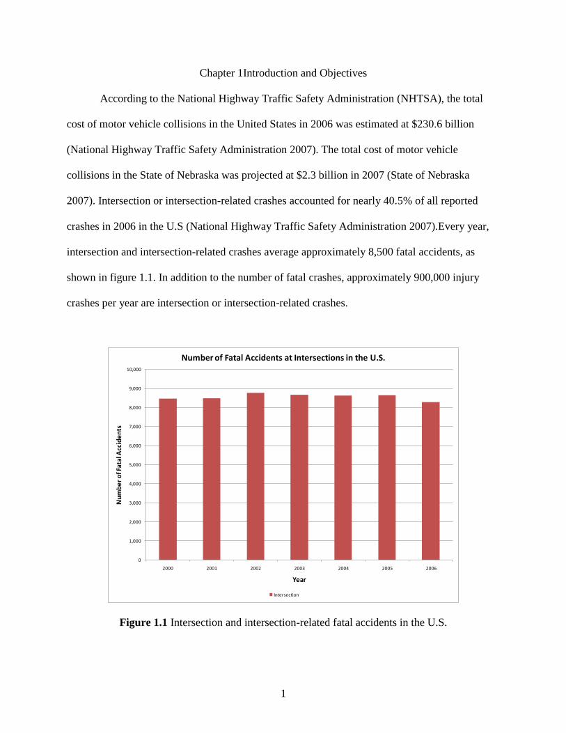
crashes in 2006 in the U.S (National Highway Traffic Safety Administration 2007).Every year,
intersection and intersection-related crashes average approximately 8,500 fatal accidents, as
shown in figure 1.1. In addition to the number of fatal crashes, approximately 900,000 injury
crashes per year are intersection or intersection-related crashes.
Figure 1.1 Intersection and intersection-related fatal accidents in the U.S.
0
1,000
2,000
3,000
4,000
5,000
6,000
7,000
8,000
9,000
10,000
2000 2001 2002 2003 2004 2005 2006
Nu
mb
er
of F
atal
Acc
ide
nts
Year
Number of Fatal Accidents at Intersections in the U.S.
Intersection
2
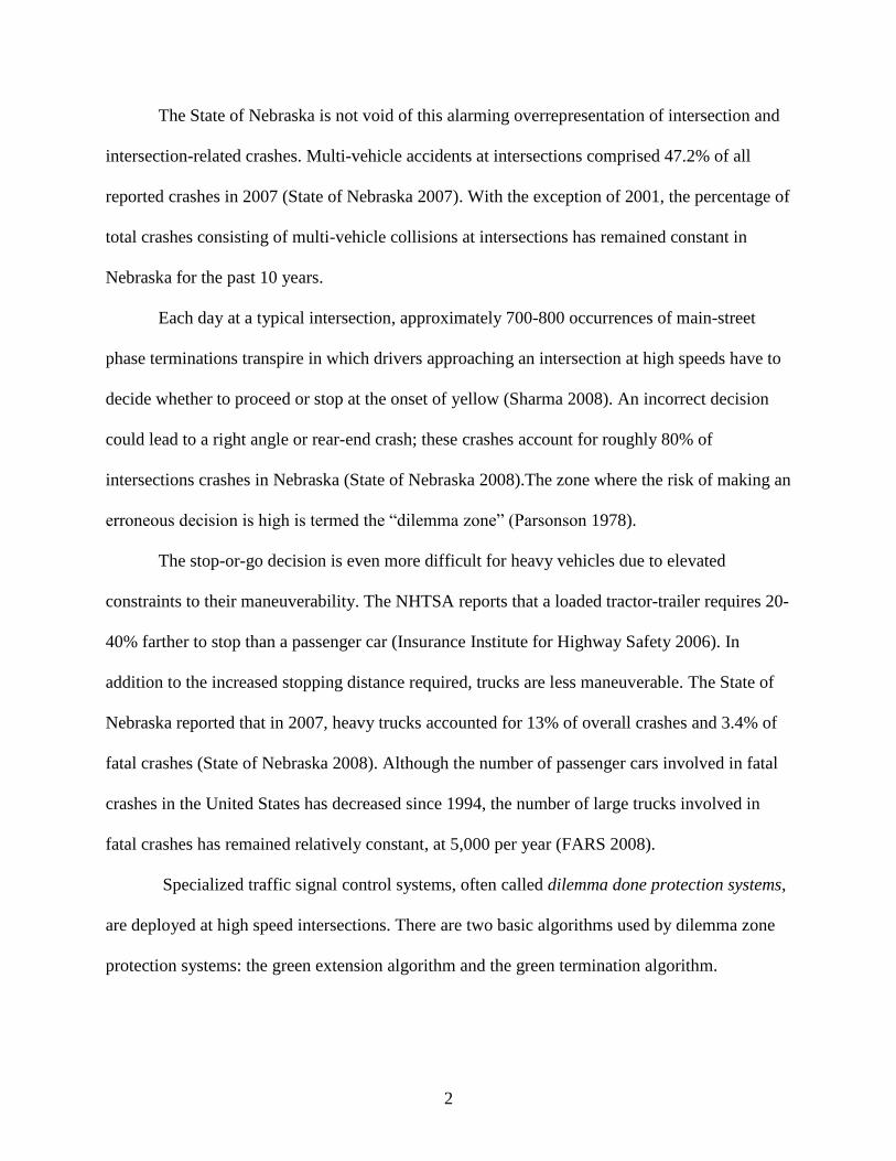
The State of Nebraska is not void of this alarming overrepresentation of intersection and
intersection-related crashes. Multi-vehicle accidents at intersections comprised 47.2% of all
reported crashes in 2007 (State of Nebraska 2007). With the exception of 2001, the percentage of
total crashes consisting of multi-vehicle collisions at intersections has remained constant in
Nebraska for the past 10 years.
Each day at a typical intersection, approximately 700-800 occurrences of main-street
phase terminations transpire in which drivers approaching an intersection at high speeds have to
decide whether to proceed or stop at the onset of yellow (Sharma 2008). An incorrect decision
could lead to a right angle or rear-end crash; these crashes account for roughly 80% of
intersections crashes in Nebraska (State of Nebraska 2008).The zone where the risk of making an
erroneous decision is high is termed the “dilemma zone” (Parsonson 1978).
The stop-or-go decision is even more difficult for heavy vehicles due to elevated
constraints to their maneuverability. The NHTSA reports that a loaded tractor-trailer requires 20-
40% farther to stop than a passenger car (Insurance Institute for Highway Safety 2006). In
addition to the increased stopping distance required, trucks are less maneuverable. The State of
Nebraska reported that in 2007, heavy trucks accounted for 13% of overall crashes and 3.4% of
fatal crashes (State of Nebraska 2008). Although the number of passenger cars involved in fatal
crashes in the United States has decreased since 1994, the number of large trucks involved in
fatal crashes has remained relatively constant, at 5,000 per year (FARS 2008).
Specialized traffic signal control systems, often called dilemma done protection systems,
are deployed at high speed intersections. There are two basic algorithms used by dilemma zone
protection systems: the green extension algorithm and the green termination algorithm.
3
Dilemma zone protection offered at high-speed intersections is based on the dilemma
zone for passenger vehicles. Federal law requires a passenger car’s brakes to sustain a minimum
deceleration rate of 21 ft/s2. A truck’s braking system is required to maintain a minimum
deceleration rate of 14 ft/s.2 Therefore, at minimum deceleration rates, a truck requires 50%
more stopping distance than a car (Federal Motor Carrier Safety Regulations 2005). Truck
drivers may be more reluctant to stop at high-speed intersections because of the increased
stopping distance or high deceleration rate required to stop. The extended amount of time
required for trucks to achieve speed prior to stopping is another possible motivation for the
reluctance to stop at such intersections.
Review of the literature confirms the deficiency of signal control strategies based
specifically on measuring truck dilemma zone boundaries. Zimmerman (2007) explored the
addition of an extended truck dilemma zone. Through the use of real-time simulation,
Zimmerman concluded that an additional 1.5 s of upstream time added to the passenger car
dilemma zone (i.e., 2.5 s-5.5 s from the stop line) would reduce the number of trucks in the
dilemma zone. The current research found that the dilemma zone boundary for heavy vehicles (3
-8.2 s from the stop line) was almost twice the dilemma zone boundary of passenger vehicles
(3.5-6 s from the stop line).
Even for passenger vehicles, the underlying concept of dilemma zone boundaries has a
serious limitation. Although dilemma zone boundaries are determined using a sound stochastic
concept, the definition of dilemma zone boundaries is still deterministic; a driver in the area
where the probability of stopping ranges from 10%-90% is considered to be unsafe, and anyone
outside of this area is considered to be safe. This binary approach states that a person is either at-
risk or risk-free—no comments are made, however, about the level of risk at each location.
4
A new and improved surrogate measure dilemma zone hazard function was recently
proposed by Sharma et al. (2007). This dilemma hazard function is a stochastic function
estimating the probability of traffic conflict of varying severity levels at a specific spatial
location.
Correct guidance for decisions at the onset of yellow can reduce the variability in driver
decision making and improve the safety of the intersection. Currently, Advance Warning
Flashers (AWF) represent the only driver assistance system in place. These systems are placed at
a fixed distance from the stop bar and activate prior to the onset of yellow. Any vehicle in
advance of the flashers is advised to stop, while any vehicle past the flashers can proceed
through the intersection. The drawbacks of these flashers are as follows:
i) Advance flashers do not account for operational differences and dilemma zone
differences occurring between different types of vehicles, providing, instead, the
same information to both cars and trucks.
ii) Vehicles traveling at different speeds incur different crash risks, but are provided
with the same information.
iii) The impact of weather and time of day is not accounted for by AWF.
iv) AWF does not consider the impact of the presence of other vehicles.
v) Personalized and dynamic information cannot be provided by AWF.
Using existing AWF systems as a test bed, the current research consisted of an in-depth
study of the role of information on driver stop-go decisions. Based on the insights gained, a
smart and dynamic yellow onset decision assist system was developed. This system was able to
cater to individual vehicle assistance needs.
5
The Yellow Onset Driver Assistance (YODA) system consisted of a pole-mounted unit
(street wave) and an in-vehicle unit. The in-vehicle unit requests decision assistance from the
pole-mounted unit as a truck approaches an intersection. Based on vehicles’ time to the stop bar
and current speed, the pole-mounted unit responds to the in-vehicle unit with a recommended
course of action. The system is a proof of concept for providing more personalized information
to the drivers.
The current report is structured as follows: chapter 2 contains a literature review of past
research pertaining to the development and advancement of dilemma zone definitions and
methods of mitigation. Past and current methods for modeling driver behavior at high-speed
intersections at the onset of yellow are presented, and the current practices involved in assessing
the safety of vehicles approaching an intersection are reviewed. The limitations of these practices
are explained.
Chapter 3 describes the six data collection sites that were utilized in the current research,
five of which had AWF and one that did not have AWF. A combination of radar-based detectors
and video was used to continuously track vehicles approaching high-speed signalized
intersections. This chapter describes the different data collection setups and details the validation
of each setup. In addition, the chapter discusses the steps taken to process the collected video.
Chapter 4 describes the theory underlying driver behavior upon approaching a signalized
intersection. The decision process of drivers at the onset of yellow was modeled using the probit
modeling technique. The impact of the role of information on driver decision making was
assessed.
Chapter 5 details the development of the prototype YODA system. The utilized
technology, codes, and testing of the prototype is described.
6
Chapter 6 summarizes study findings and proposes steps for future research. Overall, in
regards to supplementing driver decision making at high speed intersection approaches, our
findings prompt a new consideration for traffic engineers in terms of mitigating right-angle and
rear-end crash risks
7
Chapter 2 Literature Review
2.1 Introduction
The following chapter contains a literature review on past research pertaining to the
development and advancement of dilemma zone definitions and methods of risk mitigation. Past
and current methods for modeling driver behavior at high-speed intersections at the onset of
yellow are presented, as are current practices used in assessing the safety of vehicles approaching
an intersection.
2.2 Dilemma Zone Definitions
There are two distinctive types of dilemma zones: Type I and Type II. Type I dilemma
zones are caused by improper signal timing of the clearance intervals. Type II dilemma zones,
referred to as “option,” or, “indecision” zones, are caused by variance in driver behavior. The
following section will further describe the differences between the definitions of the two
commonly proposed types of dilemma zones.
2.2.1 Type I Dilemma Zone
Gazis et.al. (1960) observed problems associated with drivers facing the yellow change
interval; the authors defined the “amber light dilemma” as a situation in which a driver may be
able to neither stop safely after the onset of yellow indication nor to clear an intersection before
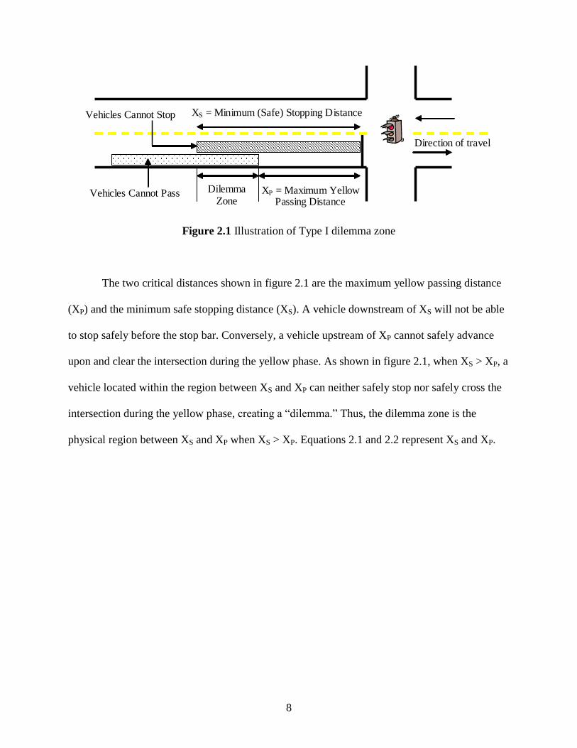
the signal turns red (Gazis et al. 1960). Figure 2.1 illustrates the concept of the Type I dilemma
zone:
8
Figure 2.1 Illustration of Type I dilemma zone
The two critical distances shown in figure 2.1 are the maximum yellow passing distance
(XP) and the minimum safe stopping distance (XS). A vehicle downstream of XS will not be able
to stop safely before the stop bar. Conversely, a vehicle upstream of XP cannot safely advance
upon and clear the intersection during the yellow phase. As shown in figure 2.1, when XS > XP, a
vehicle located within the region between XS and XP can neither safely stop nor safely cross the
intersection during the yellow phase, creating a “dilemma.” Thus, the dilemma zone is the
physical region between XS and XP when XS > XP. Equations 2.1 and 2.2 represent XS and XP.
Dilemma Zone
XP = Maximum Yellow Passing Distance
Direction of travel
Vehicles Cannot Pass
Vehicles Cannot Stop XS = Minimum (Safe) Stopping Distance
9
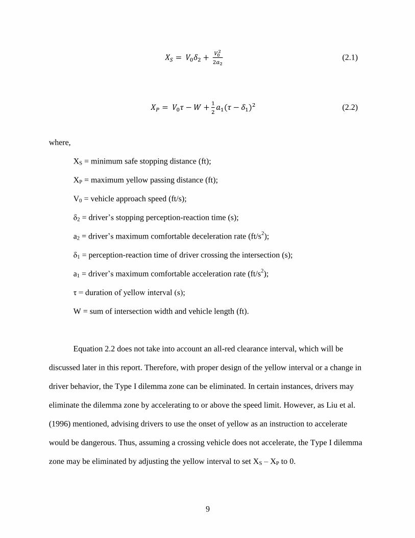
(2.1)
(2.2)
where,
XS = minimum safe stopping distance (ft);
XP = maximum yellow passing distance (ft);
V0 = vehicle approach speed (ft/s);
δ2 = driver’s stopping perception-reaction time (s);
a2 = driver’s maximum comfortable deceleration rate (ft/s2);
δ1 = perception-reaction time of driver crossing the intersection (s);
a1 = driver’s maximum comfortable acceleration rate (ft/s2);
τ = duration of yellow interval (s);
W = sum of intersection width and vehicle length (ft).
Equation 2.2 does not take into account an all-red clearance interval, which will be
discussed later in this report. Therefore, with proper design of the yellow interval or a change in
driver behavior, the Type I dilemma zone can be eliminated. In certain instances, drivers may
eliminate the dilemma zone by accelerating to or above the speed limit. However, as Liu et al.
(1996) mentioned, advising drivers to use the onset of yellow as an instruction to accelerate
would be dangerous. Thus, assuming a crossing vehicle does not accelerate, the Type I dilemma
zone may be eliminated by adjusting the yellow interval to set XS – XP to 0.
10
(2.3)
The yellow duration, τ, defined in the GHM model, has been divided into two intervals:
the yellow permissive interval, y
, and the all-red clearance interval,
.
Studies have shown a wide variability in driver behavior (Gazis et al. 1960; Olson and Rothery
1962; May 1968; Williams 1977; Parsonson and Santiago 1980; Sivak et al. 1982; Wortman and
Matthias 1983; Chang et al. 1985; Liu et al. 2007). Olson and Rothery (1962) discovered that
some drivers used the yellow interval as a green extension. May (1968) found that in an effort to
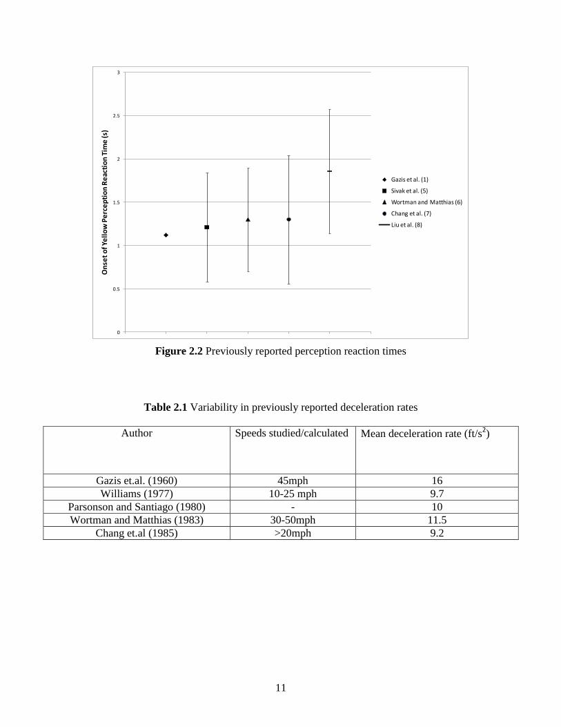
avoid the dilemma zone some drivers accelerated or decelerated heavily. Figure 2.2 and table 2.1
illustrate the variability in perception reaction times and deceleration rates at the onset of yellow.
The inability to consider variability in driver behavior variability in driver behavior is the main
limitation of the GHM model.
11
Figure 2.2 Previously reported perception reaction times
Table 2.1 Variability in previously reported deceleration rates
Author Speeds studied/calculated Mean deceleration rate (ft/s2)
Gazis et.al. (1960) 45mph 16
Williams (1977) 10-25 mph 9.7
Parsonson and Santiago (1980) - 10
Wortman and Matthias (1983) 30-50mph 11.5
Chang et.al (1985) >20mph 9.2
0
0.5
1
1.5
2
2.5
3
On
set
of Y
ell
ow
Pe
rce
pti
on
Re
acti
on
Tim
e (s
)
Gazis et al. (1)
Sivak et al. (5)
Wortman and Matthias (6)
Chang et al. (7)
Liu et al. (8)
12
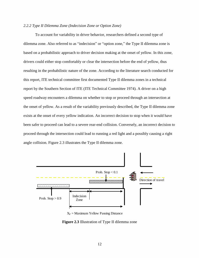
2.2.2 Type II Dilemma Zone (Indecision Zone or Option Zone)
To account for variability in driver behavior, researchers defined a second type of
dilemma zone. Also referred to as “indecision” or “option zone,” the Type II dilemma zone is
based on a probabilistic approach to driver decision making at the onset of yellow. In this zone,
drivers could either stop comfortably or clear the intersection before the end of yellow, thus
resulting in the probabilistic nature of the zone. According to the literature search conducted for
this report, ITE technical committee first documented Type II dilemma zones in a technical
report by the Southern Section of ITE (ITE Technical Committee 1974). A driver on a high
speed roadway encounters a dilemma on whether to stop or proceed through an intersection at
the onset of yellow. As a result of the variability previously described, the Type II dilemma zone
exists at the onset of every yellow indication. An incorrect decision to stop when it would have
been safer to proceed can lead to a severe rear-end collision. Conversely, an incorrect decision to
proceed through the intersection could lead to running a red light and a possibly causing a right
angle collision. Figure 2.3 illustrates the Type II dilemma zone.
Figure 2.3 Illustration of Type II dilemma zone
Indecision Zone
XP = Maximum Yellow Passing Distance
Direction of travel
Prob. Stop > 0.9
Prob. Stop < 0.1
13
Zeeger (1977) defined the type II dilemma zone as “…the road segment where more than
10 percent and less than 90 percent of the drivers would choose to stop.” Researchers have
attempted several different approaches to characterizing the indecision zone boundaries. Zeeger
(1974) used a frequency-based approach to collect data on drivers’ stopping decisions at
specified distances and speeds in order to develop a cumulative distribution function. The
dilemma zone boundaries were quantified as the distance and speed or time to the intersection.
At the onset of yellow, a driver can choose from two mutually exclusive courses of
action: stop or go. The decision process can therefore be modeled by binary discrete choice
models. Sheffi and Mahmassani (1981) modeled the driver decision process with a probit model
to significantly reduce the sample size required for estimating dilemma zone boundaries. A
driver’s perceived time to reach the stop bar, T, randomly chosen from a population, was
modeled as a random variable,
(2.4)
where,
t is the measured time to the stop bar at a constant speed;
the error term, , designating the differences in driver’s perception, is a random variable
assumed to be normally distributed.
Sheffi and Mahmassani (1981) hypothesized that drivers would choose to proceed
through the intersection if T was less than a critical value, Tcr. The critical time, Tcr, was also
modeled as a normally distributed random variable accounting for a driver’s experience,
perception of acceleration rates, and aggressiveness:
14
(2.5)
where,
tcr, is the mean critical time;
the error term, , is also normally distrusted across the driver population.
The probability of a random driver choosing to stop, PSTOP (T), is given by the probit equation:
{ } (
) (2.6)
where,
σ = √
.
In comparison to the required 2,000 observations necessary to stabilize dilemma zone
curves graphically (Mahmassani et.al. 1979), the previously described model was shown to
stabilize at approximately 150 observations. Similar results for the stability of the probit model
were demonstrated by Sharma et al. (2011)
Advantages of the model described above include the fact that dilemma zone curves are
directly calculated from the model and a small sample size of only 150 observations is required
to model dilemma zone curves
In addition to the probit model, dilemma zone boundaries have been estimated with other
models, primarily the logit model. Similar to the probit model, the logit model is a binary
discrete choice model. Recent studies using logit to develop probability of stopping curves
15
include Bonneson and Son (2003), Gates et al. (2006), Papaioannou (2007), and Kim et al
(2008). Rakha et al. (2007) used an empirical model to develop driver probability of stopping.
Elmitiny et al. (2009) used tree-based classification to model the driver stop/go decisions. As a
method of splitting data, classification trees are effective for segmenting the data into smaller
and more homogeneous groups. Elmitiny et al.(2009) split the data based on distance to the
intersection and speed at the onset of yellow; position of vehicle (leading or following); and
vehicle type. Statistical comparisons can be made based directly on the various nodes defined by
the researcher. For example, the same study revealed that drivers in the following position were
more likely to make go decisions and run the red light than were drivers in the leading position,
potentially exposing them to an increased risk of a rear-end crash.
Due to the dynamic nature of the decision dilemma zone, studies have examined
variables contributing to driver decisions to stop or proceed through the intersection. Gates et al.
(2006) observed that heavy vehicles had a higher probability than cars to proceed through the
intersection. Similar results were observed by Wei et al (2009). Sharma (2011) proposed that the
probability of stopping was a function of the acceleration required to cross the stop bar. Kim et
al. (2008) proposed that yellow-onset speed, distance from the stop line, time to stopbar, and
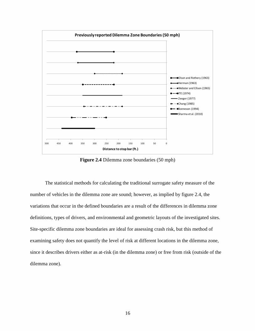
location of the signal head significantly affected driver stopping decisions. Figure 2.4 shows the
variation in the dilemma zone boundaries based on previous findings for vehicles approaching an
intersection at 50 mph.
16
Figure 2.4 Dilemma zone boundaries (50 mph)
The statistical methods for calculating the traditional surrogate safety measure of the
number of vehicles in the dilemma zone are sound; however, as implied by figure 2.4, the
variations that occur in the defined boundaries are a result of the differences in dilemma zone
definitions, types of drivers, and environmental and geometric layouts of the investigated sites.
Site-specific dilemma zone boundaries are ideal for assessing crash risk, but this method of
examining safety does not quantify the level of risk at different locations in the dilemma zone,
since it describes drivers either as at-risk (in the dilemma zone) or free from risk (outside of the
dilemma zone).
050100150200250300350400450500
Distance to stop bar (ft.)
Previously reported Dilemma Zone Boundaries (50 mph)
Olson and Rothery (1963)
Herman (1963)
Webster and Ellson (1965)
ITE (1974)
Zeeger (1977)
Chang (1985)
Bonneson (1994)
Sharma et al. (2010)
17
2.3 Effects of Yellow Length on Driver Behavior
Studies have also examined impact on driving behavior as a function of yellow interval
duration. In his comparison study of intersections equipped versus not-equipped with flashing
green, Knoflacher (1973) concluded that a decrease in right-angle crashes corresponded to
increases in the duration of yellow. The effects of yellow interval duration on stopping have also
been studied. Lengthy yellow intervals were found by Van der Horst and Wilmink (1986) to
cause poor driving behavior for last-to-stop drivers at intersections. Instead of being presented
with a red indication as they approached the stop line, drivers were stopping while the light was
still yellow; the same drivers were inclined to proceed through the intersection the next time they
approached it. Van der Horst and Wilmink (1986) found that drivers adjusted their stopping
behavior as a function of longer change intervals. The probability of stopping for drivers 4 s
from the intersection decreased from 0.5 for a yellow length of 3 s, to 0.34 for a yellow length of
5 s. Reductions in red light running (RLR) were found to decrease up to 50% for increases in
yellow ranging from 0.5-1.5 s, as long as the yellow duration did not exceed 5.5 s. Koll et al.
(2004) concluded that early stops should reduce the probability of right-angle collisions.
Contrary to the previous results, Olson and Rothery (1962) concluded that driver
behavior did not change as a function of different yellow phase durations. Studies have also
shown that overly-long amber can lead to greater variability in driver decision making, and could
potentially increases rear-end conflicts (Olson and Rothery 1962; May 1968; Mahalel and
Prashker 1987). Mahalel and Prashker (1987) noted a potential increase in the indecision zone
for a lengthy “end-of-phase” warning interval. They observed an increase in the indecision zone
with no flashing green from the normal zone of 2-5 s to a zone of 2-8 s for a 3 s yellow that was
18
preceded by a 3 s flashing green; the authors presented evidence of an increased frequency of
rear-end crashes due to the increase in the indecision zone.
2.4 Mitigation of Dilemma Zones
2.4.1 Green Extension
Advanced detection systems involve placing several loop detectors upstream of the
intersection to detect approaching vehicles and extend the green. These detectors communicate
with a computer that searches the signal controller to determine, based on vehicles’ measured
speeds, whether a green extension is required. Ideally, the green phase of the high speed
approach is extended until there is no vehicle in the dilemma zone; however, a maximum green
time is provided for this operation in order to avoid excessive delays to the cross street traffic. As
long as they are discharging at saturation flow rate, all phases are allotted green, reducing delay.
This is an all-or-nothing approach: dilemma zone protection is provided to the high speed
vehicles prior to the maximum green time being reached, at which time the protection is
removed. Developed to reduce the number of trucks being stopped at high speed rural
intersections, the Texas Transportation Institute’s (TTI) Truck Priority System is an example of a
green extension system (1997). However, the system does not specifically provide dilemma zone
protection. The system extends the phase by as much as 15 s past maximum green before
reaching max-out, at which time dilemma zone protection is removed. Another example of a
green extension system is Sweden’s LHORVA system (1993).
2.4.2 Green Termination
Green termination algorithms are relatively new, and the systems implementing them
exist at only a few intersections. These systems attempt to identify an appropriate time to end the
green phase by predicting the value of a performance function for the near future. The objective
19
is to minimize the performance function, which is based on the number of vehicles present in the
dilemma zone and the length of the opposing queue. The application of these systems has been
limited, and little quantitative data exists regarding the trade-off between efficiency, cost, and
detector requirements.
2.4.3 D-CS
Texas Transportation Institute’s Detection-Control System, or, D-CS, is a state-of-the-art
system that has been implemented at eight intersections in Texas, U.S., and three in Ontario,
Canada (2007). D-CS uses a green termination algorithm. The D-CS algorithm has two
components: vehicle status and phase status. A speed trap sufficiently distant from the
intersection (~ 800-1000 ft) is used to detect the speed and vehicle length of each vehicle. The
projected arrival and departure time of each vehicle in its respective dilemma zone (based on
speed and vehicle length) is used to maintain the “dilemma-zone matrix.” This matrix is updated
every 0.05 s. The phase status component uses the dilemma-zone matrix, maximum green time,
and number of calls registered on opposing phases to control the end time for the main street
green phase. The phase status is updated every 0.5 s.
Bonneson et al. (2005) observed reductions in the frequency of red-light violations at
almost every approach at DC-S-equipped intersections. Overall, violations were reduced by 58%,
with a reduction of about 80% for heavy vehicles. D-CS reduced violations 53% and 90% when
replacing systems that used multiple advance loop detection and systems with no advance
detection, respectively. On the approaches controlled by D-CS, severe crashes were reduced by
39%. Intersection operation improved at almost every approach at the five intersections studied.
Reductions in control delay and stop frequency were 14 % and 9 %, respectively. Most likely,
the reductions were due to D-CS’s comparative operational efficiency relative to the previous
detection and control strategies used at these intersections.
20
2.4.4 SOS – Self Optimizing Signal Control
Sweden’s SOS system is another green termination algorithm designed for isolated
intersections. Similar to D-CS, the system utilizes detectors in each lane to project the position of
vehicles as they approach the intersection. The Miller algorithm calculates the cost of ending the
green immediately or in t seconds (Kronborg 1997). Calculations are performed for different
lengths of t, for example, 0.5 s up to 20 s. The algorithm evaluates three factors: reduction in
delay and stops for vehicles using the green extension, increased delay and stops for opposing
traffic, and increased delay and stops for vehicles that cannot use the green extension and have to
wait for the next green period. In Kronborg (1997), the percentage of vehicles in the option zone
was reduced by 38%. Additionally, the number of vehicles exposed to the risk of rear-end
collision decreased by 58%.
2.4.5 Wavetronix SmartSensor Advance
Using digital wave radar, the Wavetronix SmartSensor Advance with SafeArrival
technology is one of the newest vehicle detection based systems designed to improve dilemma
zone protection (Smart Sensor Advance 2011). The system continuously tracks vehicle speed
and range to estimate the time of arrival to the stop bar. SmartSensor Advance formulates the
position and size of gaps in flowing traffic to adjust the physical location of gaps to extend the
green time if necessary to provide safe passage. In a comparison study of dilemma zone
protection systems, the Wavetronix system provided a greater reduction in the number of
vehicles in the Type II dilemma zone than did inductive loops (Knodler 2009). The SmartSensor
Advance decreased RLR incidents by more than 3 times the rate of the inductive loop system.
SmartSensor advance shows potential for early detection of heavy vehicles; this property could
be used to design different protection zones based on vehicle type.
21
2.4.6 Advance Warning
Placed upstream of high speed signalized intersections, AWF provides drivers with
information regarding whether to prepare to stop at the upcoming traffic signal or to proceed
through the intersection. Specifically, AWF is designed to minimize the number of vehicles
trapped in their respective dilemma zones at the onset of yellow (Messer 2003). AWF have been
found to improve dilemma zone protection in the state of Nebraska. McCoy and Pesti (2003)
used advanced detection and AWF to develop an enhanced dilemma zone protection system. The
system was found to reduce the number of max-outs, which result in reduced of dilemma zone
protection. Gibby et al. (1992) concluded from an analysis of high-speed signalized intersections
in California that AWF significantly reduced accident rates. Approaches having AWF displayed
lower total, left-turn, right-angle, and rear-end accident rates. Sayed et al. (1999) calculated the
reduction in total and severe accidents at intersections with AWF to be 10% and 12%,
respectively.
2.4.6.1 Advanced warning’s effects on RLR
Farraher et al. (1999) observed red light running and vehicles speeds in Bloomington,
Minnesota. Installation of AWF resulted in a 29% reduction in red light running, a 63%
reduction in truck red light running, and an 18.2% reduction in the speed of red light running
trucks. In addition, the TTI developed an Advanced Warning for End-of-Green System
(AWEGS), which utilized a sign (text or symbolic), two amber flashers, and a pair of advanced
inductive loops (Messer et al. 2003). The system, capable of identifying different classifications
of vehicles (e.g. car, truck), has been found to decrease delay due to stoppages at traffic signals
and provide extra dilemma zone protection for high-speed vehicles and trucks. Results showed a
reduction in RLR by 38%-42% percent in the first 5 s of red.
22
Although the consensus surrounding AWF is that the system provides safety benefits,
several concerns have also been raised. For example, Farraher et al. (1999) detected that drivers
running red lights entered speeds above the speed limit, increasing the risk of crash for opposing
traffic. Pant and Huang (1992) evaluated several high-speed intersections with AWF, detecting
increases in vehicle speed as traffic signals approached the red phase; thus, the authors
discouraged the use of Prepare to Stop When Flashing (PTSWF) and Flashing Symbolic Signal
Ahead (FSSA) signs along tangent intersection approaches. Further testing performed by Pant
and Xie (1995) at two intersections verified these findings.
Flashing green systems are similar to AWF systems, and have been implemented and
tested thoroughly in Europe and Israel. Knoflacher (1973) studied decelerations and accidents at
intersections equipped with and without flashing green systems, finding that intersections
implemented with flashing green systems had higher deceleration rates and increases in the
number of rear-end collisions. In a simulated study comparing driver responses at intersections
with flashing green, Mahalel et al. (1985) noted a significant increase in erroneous decisions at
the onset of yellow. In particular, inappropriate stop decisions at intersections with flashing
green doubled to 77% in comparison to the 38% observed at intersections lacking the flashing
green interval. This increase in inappropriate stops caused a considerable shift in the probability
of stopping curves. Koll et al. (2004) compared the effects of flashing green on 10 approaches in
Austria, Switzerland, and Germany. The examined safety impact was the amount of yellow and
red stop line crossings observed. A substantial increase in the number of early stops was found in
Austria. A larger option zone (an area where drivers could both proceed or stop safely) increased
as a result.
23
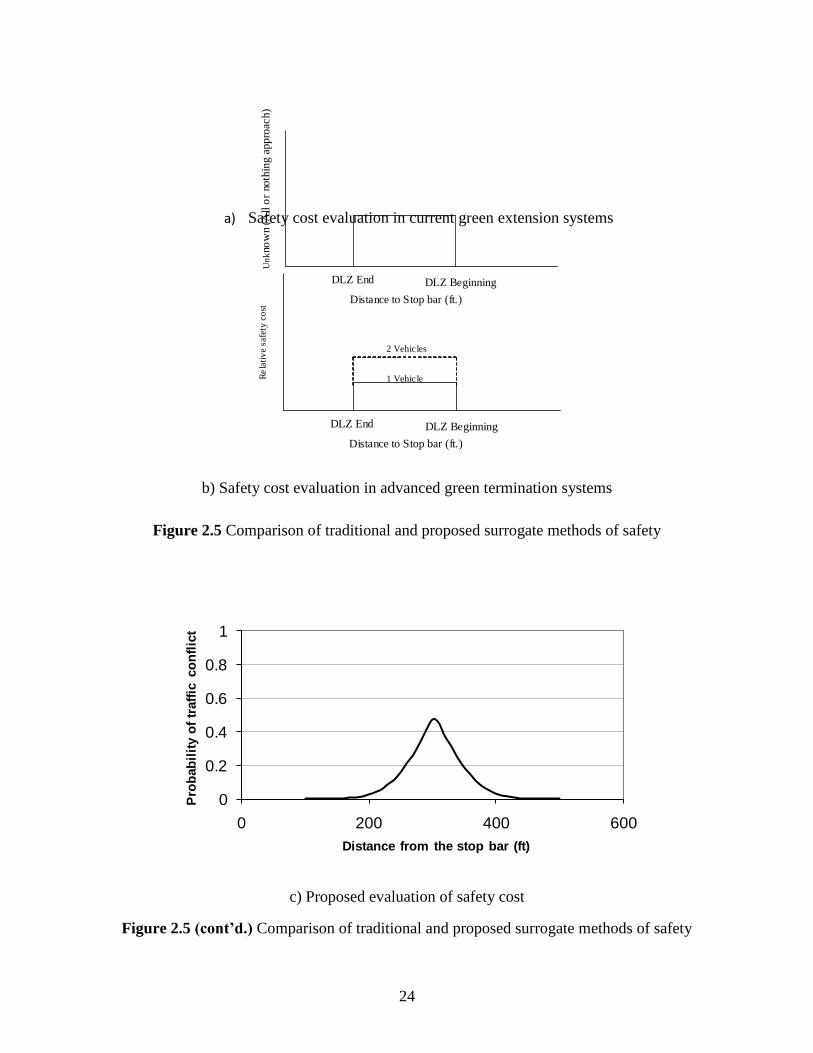
2.5 Traffic Conflicts
As previously mentioned, traditional surrogate measures of safety (such as the number of
vehicles in the dilemma zone) fail to quantify the risk of a crash. Meanwhile, traffic conflicts
have demonstrated usefulness as indirect measures with which to evaluate the safety of an
intersection. Figures 2.6a to 2.6c contrast the present surrogate measure of safety with the
proposed surrogate measure of safety. Widely used green extension systems are all-or-nothing
approaches: all vehicles on the high-speed approaches are cleared until the maximum green time
is reached, but at the end of the maximum green time, none of the vehicles on the high-speed
approach are protected. As shown in figure 2.5a, these systems do not include a metric to
measure the cost of the risk of crash. Green termination systems use the number of vehicles in
the dilemma zone as a surrogate measure for quantifying the cost of risk. The number of vehicles
is a rank-ordered metric, shown in figure 2.5b, where the cost of one vehicle in the dilemma zone
is less than the cost of two vehicles in the dilemma zone; but the cost is independent of the
positions of vehicles in the dilemma zone. Sharma (2011) modeled the dilemma zone hazard
using the observed probability of stop and go at the onset of yellow. The probability of making
an erroneous decision was used as the probability of traffic conflict. Dilemma hazard functions
obtained for vehicles traveling at 45 mph, as estimated for the study site at Noblesville, IN, are
shown in figure 2.5c. The probability of conflict curves developed by Sharma included single
passenger vehicles only. The current research develops the dilemma hazard function for heavy
vehicles. It should be noted that the dilemma hazard function can be further enhanced by adding
severe conflict boundaries using acceleration and deceleration thresholds.
24
a) Safety cost evaluation in current green extension systems
b) Safety cost evaluation in advanced green termination systems
Figure 2.5 Comparison of traditional and proposed surrogate methods of safety
c) Proposed evaluation of safety cost
Figure 2.5 (cont’d.) Comparison of traditional and proposed surrogate methods of safety
0
0.2
0.4
0.6
0.8
1
0 200 400 600
Pro
bab
ilit
y o
f tr
aff
ic c
on
flic
t
Distance from the stop bar (ft)
DLZ End DLZ Beginning
Distance to Stop bar (ft.)
Un
kno
wn
(All o
r no
thin
g a
pp
roac
h)
DLZ End DLZ Beginning
Distance to Stop bar (ft.)
Re
lati
ve
safe
ty c
ost
1 Vehicle
2 Vehicles
25
2.5.1 Traffic Conflict Technique
Over the past four decades, the traffic conflict technique (TCT) has evolved,
demonstrating its usefulness for indirectly evaluating the safety of intersections. The technique
originated from research performed at the General Motors laboratory in Detroit, MI, being used
to identify safety problems relating to vehicle construction. Perkins and Harris (1968) defined a
conflict as “The occurrence of evasive actions, such as braking or weaving, which are forced on
the driver by an impending crash situation or a traffic violation;” they categorized the conflicts
into left-turn conflicts, cross-traffic conflicts, weave conflicts, and rear-end conflicts.
TCT gained popularity as research efforts attempted to establish a direct relationship
between conflicts and crashes (Baker 1972; Spicer 1972; Cooper 1973; Paddock 1974). Research
has made clear that conflict data is a much faster method of data collection than waiting for an
actual crash history to develop; for this reason, conflict data, as opposed to crash data, allows
researcher to make a determination regarding the safety of a specific intersection rather rapidly.
This allows for information regarding the safety of an intersection to be collected rather quickly.
Cooper and Ferguson (1976) calculated the ratio of the rate of serious conflicts to the rate of
crashes, deriving a figure of approximately 2,000:1. A recent study by the FHWA (2008) found
the ratio of traffic conflicts to actual crashes to be approximately 20,000:1. In addition to more
rapid data collection, TCT facilitates the quick identification of the safety deficiencies at
intersections. Thus, TCT allows traffic engineers the opportunity to provide proactive safety
improvements at intersections instead of waiting for crash histories to evolve.
Questions regarding TCT have been raised by several researchers. Glennon et al. (1977)
expressed concern over the use of the TCT technique, stating that the reliability of TCT for
estimating crash potential is questionable. The same authors found that for every study in favor
26
of TCT, there was a study that opposed it; they argued that the ability to predict the number of
crashes at an intersection was extremely improbable given that conflicts and crashes are random
events.
Although concerns have been raised regarding the use of TCT, recent studies have
continued to advocate its use as a surrogate measure of safety. Glauz et al. (1985) investigated
two types of expected crash prediction rates, one based on conflict ratios and the other based on
crash histories. The study determined the difference to be statistically insignificant; thus, an
estimate of the expected crash rates using traffic conflicts can be as accurate and precise as an
estimate predicted by crash history. Hyden (1987) concluded that conflicts and crashes did in
fact share the same severity distribution based on time-to-accident (TA) and speed values. The
use of traffic conflict as a surrogate measure for traffic safety in micro-simulation has been
advocated by Fazio et al. (1993), and by Gettman and Head (2003), who performed a detailed
use-case analysis.
2.5.2 Traffic Conflicts at the Onset of Yellow
Zeeger (1977) identified six conflicts that can occur at the onset of yellow. The following
definitions of the six conflicts were used during the conflict analysis performed as part of this
report:
Red light runner (RLR): A red light violation was defined as occurring when the front
of the vehicle was behind the stop line at the onset of red.
Abrupt stop: An abrupt stop occurs when a vehicle could successfully clear the
intersection but decides to stop. Abrupt stop conflicts can be viewed visually and
calculated mathematically based on the onset of yellow distance and speed.
27
Swerve-to-avoid collision: Classified as an erratic maneuver that occurs when a
driver swerves out of their lane to avoid hitting the vehicle stopped at the light in
front of them.
Vehicle skidded: This is a more severe case of an abrupt stop where the vehicle’s
wheels “lock-up” in order to stop. This conflict can be heard audibly.
Acceleration through yellow: Acceleration through yellow is identified either by
being heard audibly or through mathematical calculation. Each vehicle’s distance is
projected at the onset of red based on the onset of yellow distance and vehicle speed,
assuming constant speed. Acceleration through yellow conflict is assigned if the
vehicle successfully crosses the stop bar but would not have done so if based on the
constant speed projection.
Brakes applied before passing through: This conflict can be viewed visually when, at
the onset of yellow, the driver applied the brakes before passing through the
intersection. It indicates the indecisiveness of drivers when approaching the
intersection.
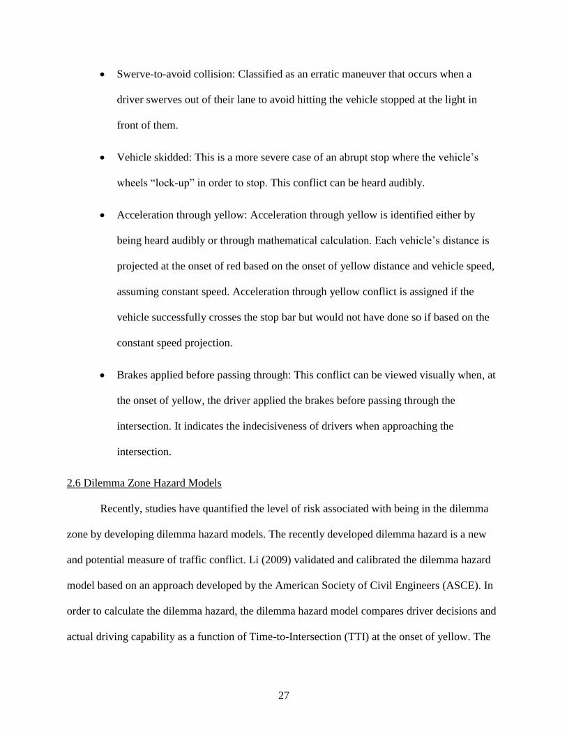
2.6 Dilemma Zone Hazard Models
Recently, studies have quantified the level of risk associated with being in the dilemma
zone by developing dilemma hazard models. The recently developed dilemma hazard is a new
and potential measure of traffic conflict. Li (2009) validated and calibrated the dilemma hazard
model based on an approach developed by the American Society of Civil Engineers (ASCE). In
order to calculate the dilemma hazard, the dilemma hazard model compares driver decisions and
actual driving capability as a function of Time-to-Intersection (TTI) at the onset of yellow. The
28
approach uses driver decisions at the onset of yellow, their actual capabilities based on vehicle
kinematics, and previously reported acceleration and deceleration rates. The collected data was
simulated using Monte Carlo simulation to establish dilemma hazard values within the dilemma
zone boundaries of 2-5 s (Li 2009). Models were created for single vehicle and multiple (two)
vehicle scenarios. Results of the simulation, shown in figure 2.6, illustrate the effect of signal
timings on the dilemma hazard.
Figure 2.6 Dilemma hazard curves for various yellow and all-red clearance intervals (Li 2009)
Sharma et al. (2011) provided theoretical justification for using the probability of
stopping to estimate the probability of conflict for single vehicles at high-speed intersections. A
detailed discussion of this topic is provided in the following chapter.
29
2.7 Summary
The development of knowledge regarding dilemma zones and traffic conflicts has
continuously progressed. The traditional surrogate measure of safety—the dilemma zone—
denotes the region of risk, but does not quantify the level of risk. Recently, the dilemma hazard
model and dilemma hazard function have attempted to quantify the level of risk associated with
being in the dilemma zone at the onset of yellow. The current study aimed to identify the impact
of providing additional information on driver stop and go decision making. The insights gained
were used to develop the prototype YODA system.
30
Chapter 3 Data Collection
3.1 Introduction
To achieve as thorough an analysis as possible, five locations were selected for data
collection, and a sixth site was evaluated for comparison. A combination of radar based detectors
and video was used to continuously track vehicles approaching high-speed signalized
intersections. This chapter describes the data collection locations, equipment setup and
calibration, and video processing tasks.
3.2 Data Collection Sites
This section describes the six studied intersections:
3.2.1 US 77 and Saltillo Rd.
The first intersection studied was the northbound approach of US 77 and Saltillo Rd.
Located east of Lincoln, Nebraska, US Highway 77 runs north and south. The intersection has
two through lanes and both a left and right turn lane. Two PTSWF flashers are positioned on
both sides of US 77, 650 ft. from the stop bar. The speed limit is 65 mph until approximately
1,150 ft. before the intersection, when the speed limit changes to 55 mph.
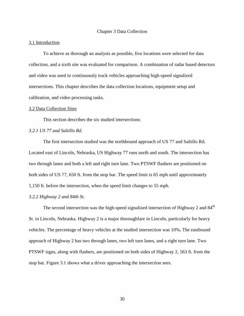
3.2.2 Highway 2 and 84th St.
The second intersection was the high-speed signalized intersection of Highway 2 and 84th
St. in Lincoln, Nebraska. Highway 2 is a major thoroughfare in Lincoln, particularly for heavy
vehicles. The percentage of heavy vehicles at the studied intersection was 10%. The eastbound
approach of Highway 2 has two through lanes, two left turn lanes, and a right turn lane. Two
PTSWF signs, along with flashers, are positioned on both sides of Highway 2, 563 ft. from the
stop bar. Figure 3.1 shows what a driver approaching the intersection sees.
31
Figure 3.1 View of advance warning flashers prior to intersection
3.2.3 US 77 and Pioneers
US 77 and Pioneers Blvd., located five miles north of US 77 and Saltillo, was the third
intersection studied. The southbound approach of US 77 and Pioneers has two through lanes and
one left turn lane. Two PTSWF flashers are positioned on both sides of US 77, 650 ft. from the
stop bar. The speed limit is 55 mph along this stretch of US 77.
3.2.4 Highway 34 and N79
The last intersection studied in Lincoln was the westbound approach of Highway 34 and
N 79. This intersection is northwest of Lincoln, with a speed limit of 60 mph. With no left turn
lane and a turnoff for vehicles desiring to travel north prior to the intersection, the westbound
approach has only two through lanes. In addition, the intersection is equipped with two PTSWF
flashers, 650 ft. from the stop bar.
32
3.2.5 Highway 75 and Platteview Rd.
Shown in figure 3.2 US 75 and Platteview Road, is located south of Bellevue, Nebraska.
The southbound approach of US 75 and Platteview has two through lanes and both a right and
left turn lane. Two PTWSF flashers are positioned on both sides of US 75, 438 ft. from the stop
bar. Approximately 1,550 ft. upstream of the intersection, the speed limit changes from 60 mph
to 55 mph.
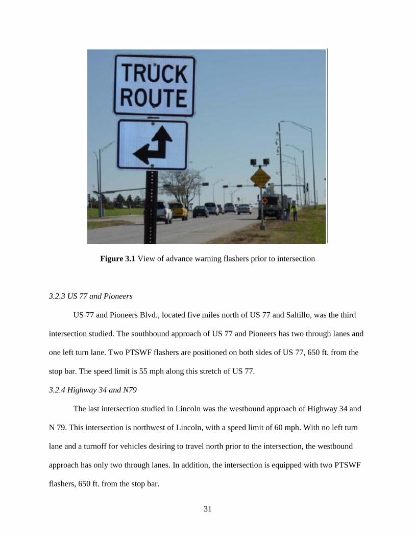
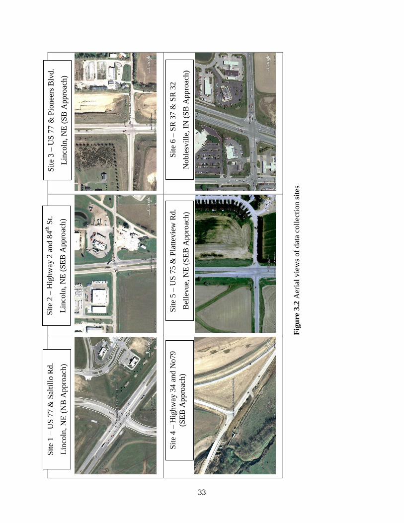
3.2.6 SR32 and SR 37
The last site used for data analysis was the signalized intersection of SR 37 and SR 32 at
Noblesville, Indiana. The southbound approach of SR 37 has two through lanes and both a right
and left turn lane. The speed limit of SR 37 is 55 mph. Unlike the other five sites, this
intersection does not have advance warning flashers. In addition, the wide area detectors (WAD)
and camera were mounted on the mast arm, contrasting the previous locations that were on the
side of the road.
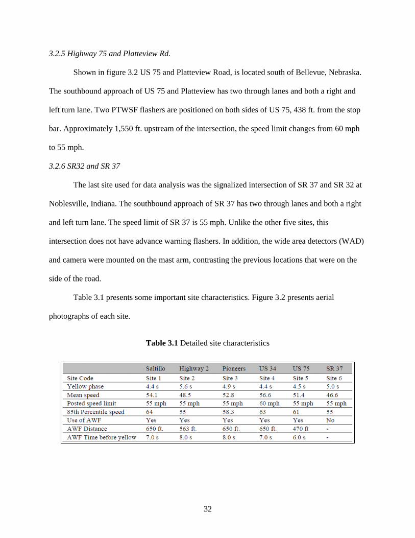
Table 3.1 presents some important site characteristics. Figure 3.2 presents aerial
photographs of each site.
Table 3.1 Detailed site characteristics
Fig
ure
3.2
Aer
ial
vie
ws
of
dat
a co
llec
tion s
ites
Sit
e 2 –
Hig
hw
ay 2
and 8
4th
St.
Lin
coln
, N
E (
SE
B A
pp
roac
h)
Sit
e 1 –
US
77 &
Sal
till
o R
d.
Lin
coln
, N
E (
NB
Appro
ach)
Sit
e 4 –
Hig
hw
ay 3
4 a
nd N
o79
(SE
B A
ppro
ach)
Sit
e 5 –
US
75 &
Pla
ttev
iew
Rd.
Bel
levue,
NE
(S
EB
Appro
ach)
Sit
e 3 –
US
77 &
Pio
nee
rs B
lvd.
Lin
coln
, N
E (
SB
App
roac
h)
Sit
e 6 –
SR
37 &
SR
32
Noble
svil
le,
IN (
SB
App
roac
h)
33
34
3.3 Data Collection
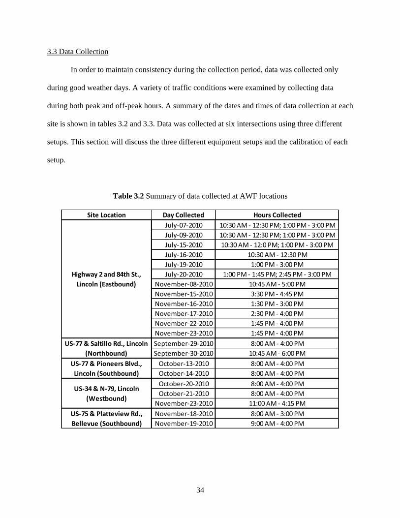
In order to maintain consistency during the collection period, data was collected only
during good weather days. A variety of traffic conditions were examined by collecting data
during both peak and off-peak hours. A summary of the dates and times of data collection at each
site is shown in tables 3.2 and 3.3. Data was collected at six intersections using three different
setups. This section will discuss the three different equipment setups and the calibration of each
setup.
Table 3.2 Summary of data collected at AWF locations
Site Location Day Collected Hours Collected
July-07-2010 10:30 AM - 12:30 PM; 1:00 PM - 3:00 PM
July-09-2010 10:30 AM - 12:30 PM; 1:00 PM - 3:00 PM
July-15-2010 10:30 AM - 12:0 PM; 1:00 PM - 3:00 PM
July-16-2010 10:30 AM - 12:30 PM
July-19-2010 1:00 PM - 3:00 PM
July-20-2010 1:00 PM - 1:45 PM; 2:45 PM - 3:00 PM
November-08-2010 10:45 AM - 5:00 PM
November-15-2010 3:30 PM - 4:45 PM
November-16-2010 1:30 PM - 3:00 PM
November-17-2010 2:30 PM - 4:00 PM
November-22-2010 1:45 PM - 4:00 PM
November-23-2010 1:45 PM - 4:00 PM
September-29-2010 8:00 AM - 4:00 PM
September-30-2010 10:45 AM - 6:00 PM
October-13-2010 8:00 AM - 4:00 PM
October-14-2010 8:00 AM - 4:00 PM
October-20-2010 8:00 AM - 4:00 PM
October-21-2010 8:00 AM - 4:00 PM
November-23-2010 11:00 AM - 4:15 PM
November-18-2010 8:00 AM - 3:00 PM
November-19-2010 9:00 AM - 4:00 PM
US-77 & Saltillo Rd., Lincoln
(Northbound)
US-77 & Pioneers Blvd.,
Lincoln (Southbound)
US-34 & N-79, Lincoln
(Westbound)
Highway 2 and 84th St.,
Lincoln (Eastbound)
US-75 & Platteview Rd.,
Bellevue (Southbound)
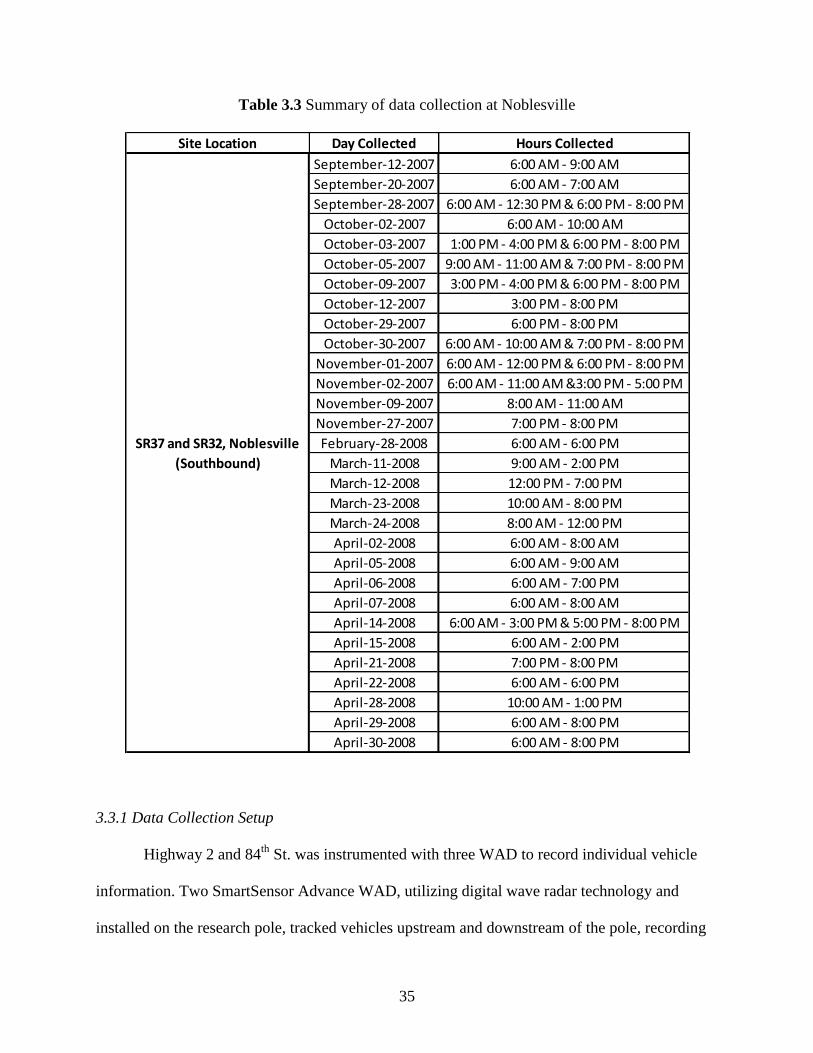
35
Table 3.3 Summary of data collection at Noblesville
3.3.1 Data Collection Setup
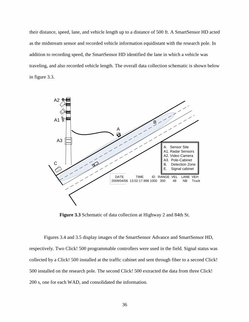
Highway 2 and 84th
St. was instrumented with three WAD to record individual vehicle
information. Two SmartSensor Advance WAD, utilizing digital wave radar technology and
installed on the research pole, tracked vehicles upstream and downstream of the pole, recording
Site Location Day Collected Hours Collected
September-12-2007 6:00 AM - 9:00 AM
September-20-2007 6:00 AM - 7:00 AM
September-28-2007 6:00 AM - 12:30 PM & 6:00 PM - 8:00 PM
October-02-2007 6:00 AM - 10:00 AM
October-03-2007 1:00 PM - 4:00 PM & 6:00 PM - 8:00 PM
October-05-2007 9:00 AM - 11:00 AM & 7:00 PM - 8:00 PM
October-09-2007 3:00 PM - 4:00 PM & 6:00 PM - 8:00 PM
October-12-2007 3:00 PM - 8:00 PM
October-29-2007 6:00 PM - 8:00 PM
October-30-2007 6:00 AM - 10:00 AM & 7:00 PM - 8:00 PM
November-01-2007 6:00 AM - 12:00 PM & 6:00 PM - 8:00 PM
November-02-2007 6:00 AM - 11:00 AM &3:00 PM - 5:00 PM
November-09-2007 8:00 AM - 11:00 AM
November-27-2007 7:00 PM - 8:00 PM
February-28-2008 6:00 AM - 6:00 PM
March-11-2008 9:00 AM - 2:00 PM
March-12-2008 12:00 PM - 7:00 PM
March-23-2008 10:00 AM - 8:00 PM
March-24-2008 8:00 AM - 12:00 PM
April-02-2008 6:00 AM - 8:00 AM
April-05-2008 6:00 AM - 9:00 AM
April-06-2008 6:00 AM - 7:00 PM
April-07-2008 6:00 AM - 8:00 AM
April-14-2008 6:00 AM - 3:00 PM & 5:00 PM - 8:00 PM
April-15-2008 6:00 AM - 2:00 PM
April-21-2008 7:00 PM - 8:00 PM
April-22-2008 6:00 AM - 6:00 PM
April-28-2008 10:00 AM - 1:00 PM
April-29-2008 6:00 AM - 8:00 PM
April-30-2008 6:00 AM - 8:00 PM
SR37 and SR32, Noblesville
(Southbound)
36
their distance, speed, lane, and vehicle length up to a distance of 500 ft. A SmartSensor HD acted
as the midstream sensor and recorded vehicle information equidistant with the research pole. In
addition to recording speed, the SmartSensor HD identified the lane in which a vehicle was
traveling, and also recorded vehicle length. The overall data collection schematic is shown below
in figure 3.3.
Figure 3.3 Schematic of data collection at Highway 2 and 84th St.
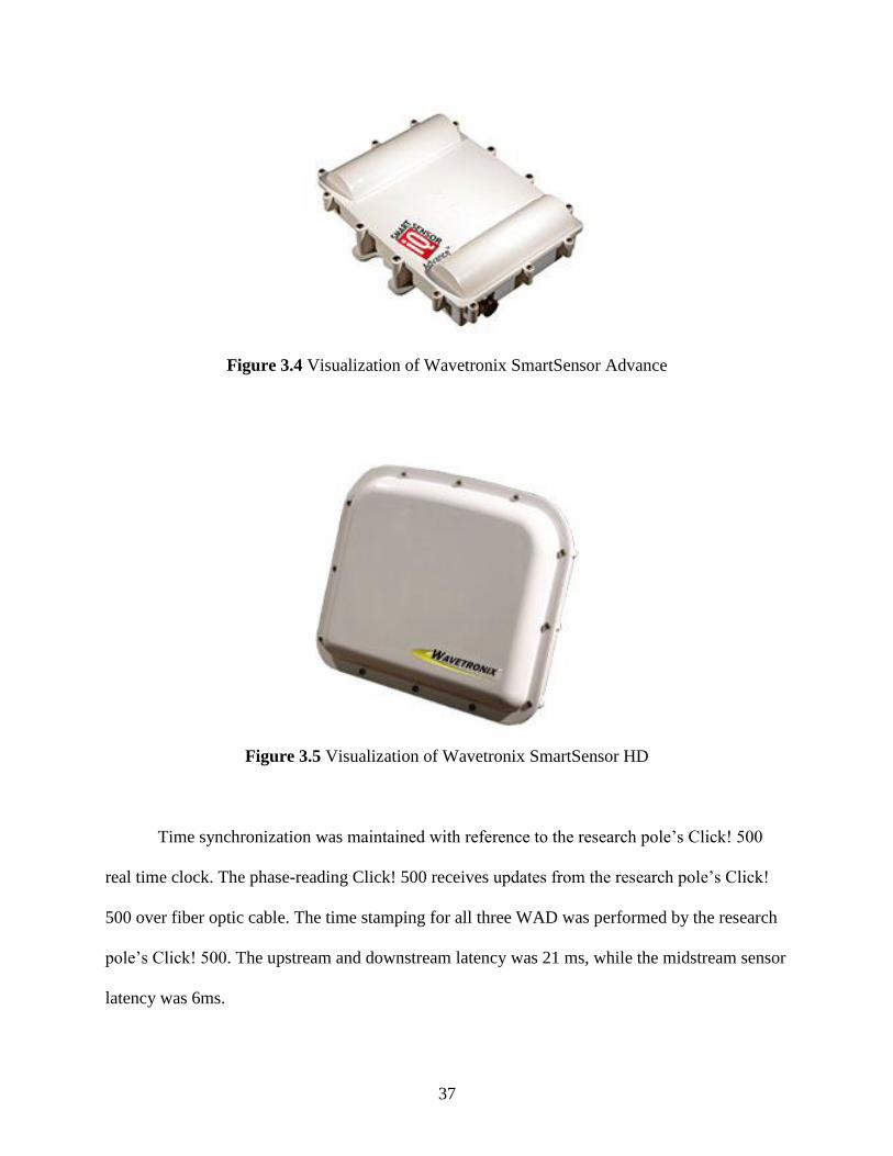
Figures 3.4 and 3.5 display images of the SmartSensor Advance and SmartSensor HD,
respectively. Two Click! 500 programmable controllers were used in the field. Signal status was
collected by a Click! 500 installed at the traffic cabinet and sent through fiber to a second Click!
500 installed on the research pole. The second Click! 500 extracted the data from three Click!
200 s, one for each WAD, and consolidated the information.
A. Sensor Site
A1. Radar Sensors
A2. Video Camera
A3. Pole-Cabinet
B. Detection Zone
E. Signal cabinet
B
A
A1
A2
A3
C
DATE TIME ID RANGE VEL LANE VEH
2009/04/06 13:02:17.998 1000 300 48 NB Truck
37
Figure 3.4 Visualization of Wavetronix SmartSensor Advance
Figure 3.5 Visualization of Wavetronix SmartSensor HD
Time synchronization was maintained with reference to the research pole’s Click! 500
real time clock. The phase-reading Click! 500 receives updates from the research pole’s Click!
500 over fiber optic cable. The time stamping for all three WAD was performed by the research
pole’s Click! 500. The upstream and downstream latency was 21 ms, while the midstream sensor
latency was 6ms.
38
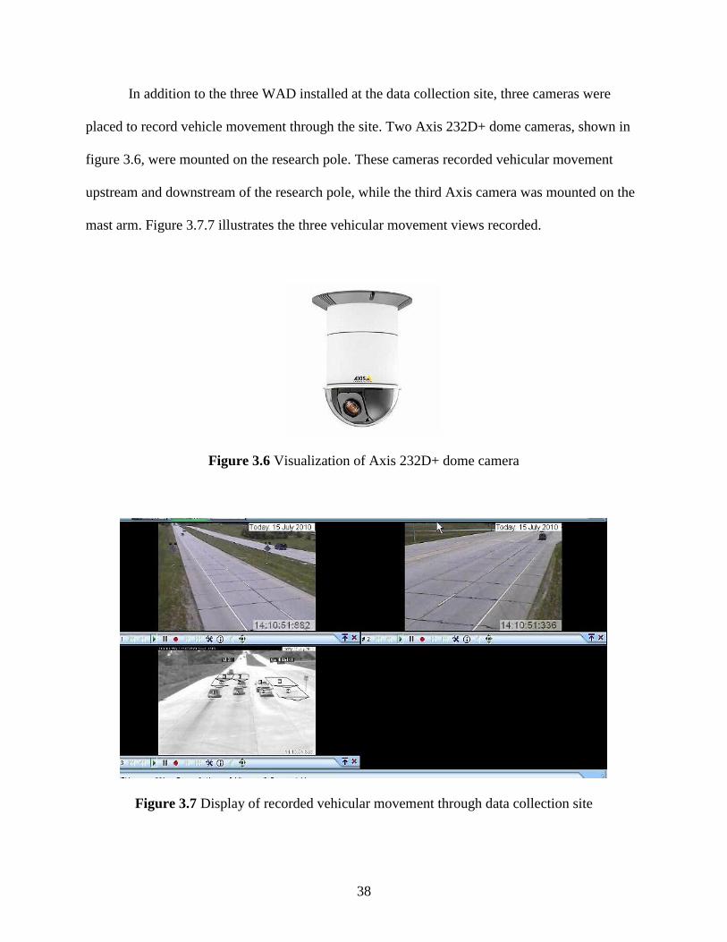
In addition to the three WAD installed at the data collection site, three cameras were
placed to record vehicle movement through the site. Two Axis 232D+ dome cameras, shown in
figure 3.6, were mounted on the research pole. These cameras recorded vehicular movement
upstream and downstream of the research pole, while the third Axis camera was mounted on the
mast arm. Figure 3.7.7 illustrates the three vehicular movement views recorded.
Figure 3.6 Visualization of Axis 232D+ dome camera
Figure 3.7 Display of recorded vehicular movement through data collection site
39
Data from the WAD was collected through placing a serial cable connecting the RS-232
on the Click! 500 to a CPU in the research pole. Matlab was used to open the serial connection
and save the data. The three cameras were displayed on the computer screen using Active
Webcam, which captured images at up to 30 fps. Finally, Hypercam 2 was used to record the
screen captures from Active Webcam, as shown in figure 3.7.
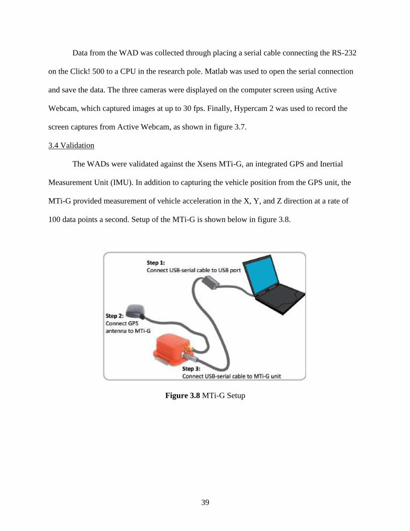
3.4 Validation
The WADs were validated against the Xsens MTi-G, an integrated GPS and Inertial
Measurement Unit (IMU). In addition to capturing the vehicle position from the GPS unit, the
MTi-G provided measurement of vehicle acceleration in the X, Y, and Z direction at a rate of
100 data points a second. Setup of the MTi-G is shown below in figure 3.8.
Figure 3.8 MTi-G Setup
40
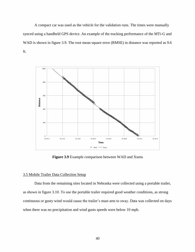
A compact car was used as the vehicle for the validation runs. The times were manually
synced using a handheld GPS device. An example of the tracking performance of the MTi-G and
WAD is shown in figure 3.9. The root mean square error (RMSE) in distance was reported as 9.6
ft.
Figure 3.9 Example comparison between WAD and Xsens
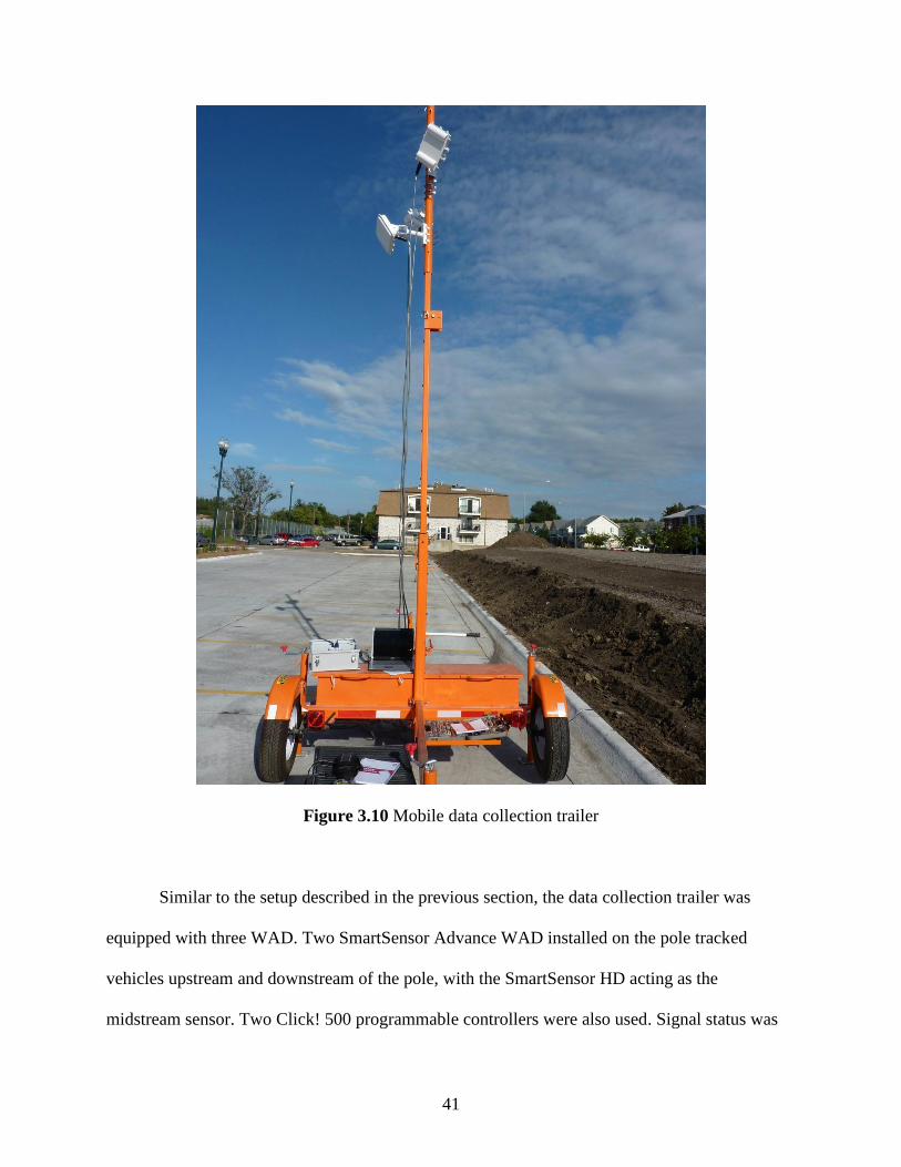
3.5 Mobile Trailer Data Collection Setup
Data from the remaining sites located in Nebraska were collected using a portable trailer,
as shown in figure 3.10. To use the portable trailer required good weather conditions, as strong
continuous or gusty wind would cause the trailer’s mast arm to sway. Data was collected on days
when there was no precipitation and wind gusts speeds were below 10 mph.
0
200
400
600
800
1000
51:07.2 51:11.5 51:15.8 51:20.2 51:24.5 51:28.8 51:33.1 51:37.4
Dis
tan
ce
Time
WAD Xsens
41
Figure 3.10 Mobile data collection trailer
Similar to the setup described in the previous section, the data collection trailer was
equipped with three WAD. Two SmartSensor Advance WAD installed on the pole tracked
vehicles upstream and downstream of the pole, with the SmartSensor HD acting as the
midstream sensor. Two Click! 500 programmable controllers were also used. Signal status was
42
received from the Click! 500 installed at the traffic cabinet through the portable signal phase
reader, shown below in figure 3.11.
Figure 3.11 Safe Track portable signal phase reader
43
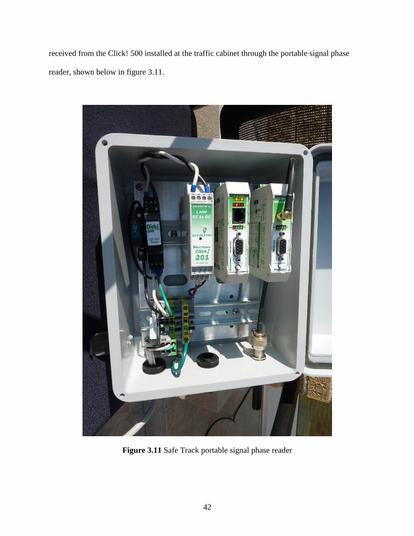
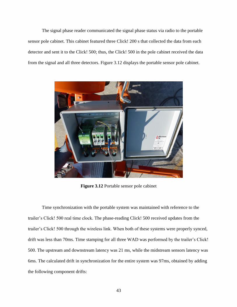
The signal phase reader communicated the signal phase status via radio to the portable
sensor pole cabinet. This cabinet featured three Click! 200 s that collected the data from each
detector and sent it to the Click! 500; thus, the Click! 500 in the pole cabinet received the data
from the signal and all three detectors. Figure 3.12 displays the portable sensor pole cabinet.
Figure 3.12 Portable sensor pole cabinet
Time synchronization with the portable system was maintained with reference to the
trailer’s Click! 500 real time clock. The phase-reading Click! 500 received updates from the
trailer’s Click! 500 through the wireless link. When both of these systems were properly synced,
drift was less than 70ms. Time stamping for all three WAD was performed by the trailer’s Click!
500. The upstream and downstream latency was 21 ms, while the midstream sensors latency was
6ms. The calculated drift in synchronization for the entire system was 97ms, obtained by adding
the following component drifts:
44
70ms for the phase information
21 ms for the upstream and downstream sensor
6ms for the midstream sensor
The entire system had a time resolution accuracy of at least 1/10
th of a second. The data
was pushed from the Click! 500 using the device’s serial port and a serial to USB converter that
connected to a laptop. Matlab opened the serial port and saved the data in both .DAT and .txt
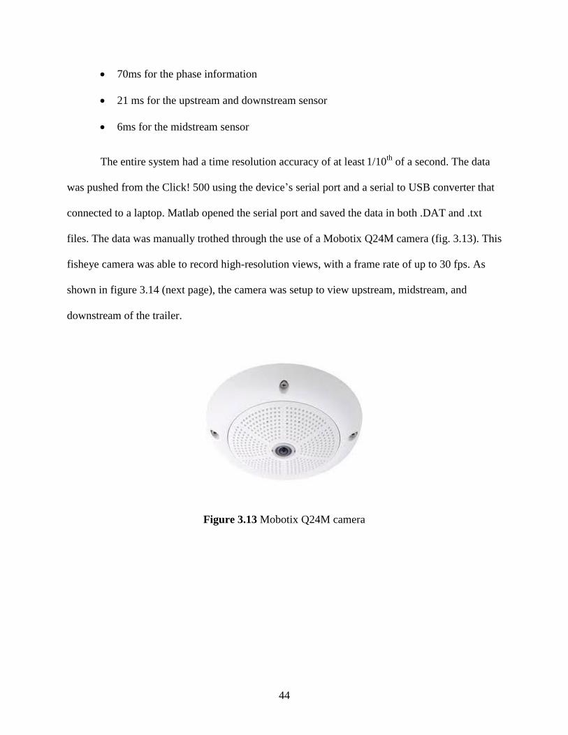
files. The data was manually trothed through the use of a Mobotix Q24M camera (fig. 3.13). This
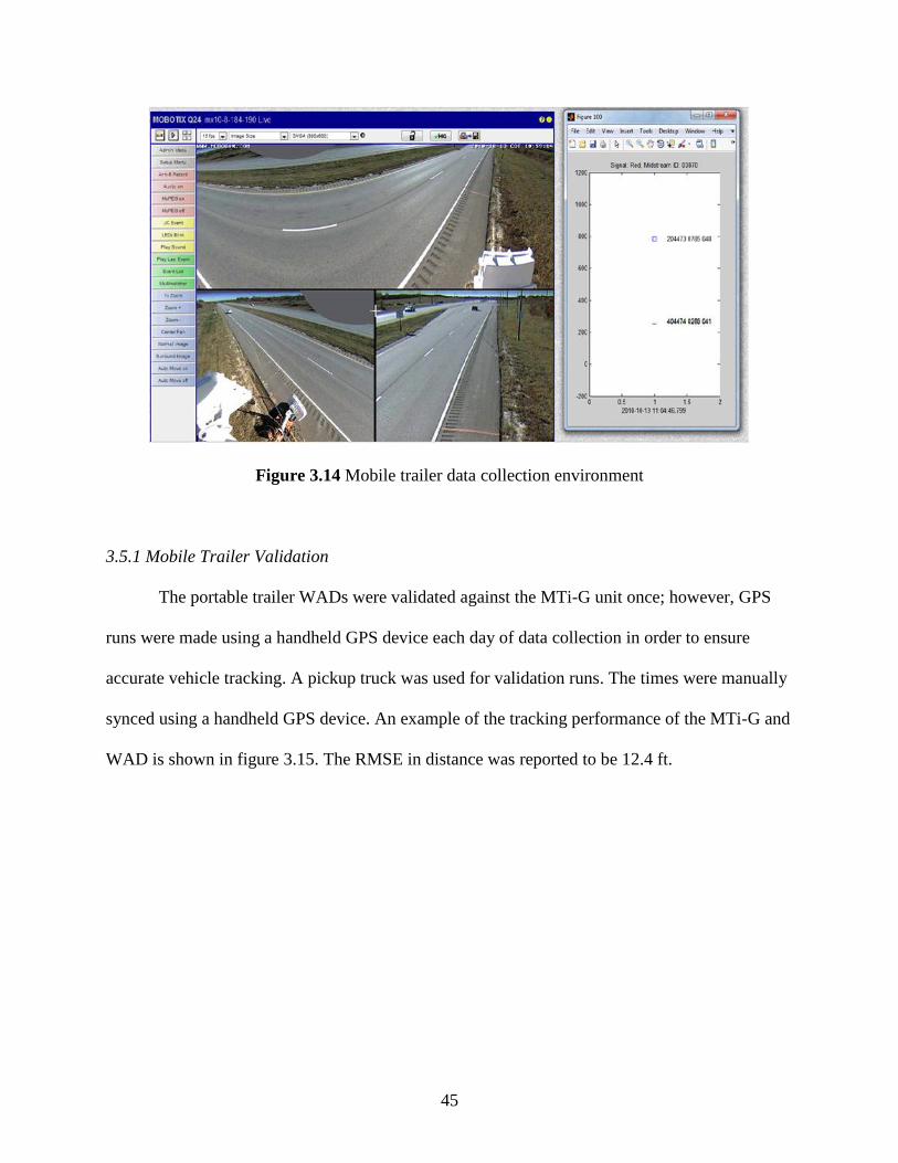
fisheye camera was able to record high-resolution views, with a frame rate of up to 30 fps. As
shown in figure 3.14 (next page), the camera was setup to view upstream, midstream, and
downstream of the trailer.
Figure 3.13 Mobotix Q24M camera
45
Figure 3.14 Mobile trailer data collection environment
3.5.1 Mobile Trailer Validation
The portable trailer WADs were validated against the MTi-G unit once; however, GPS
runs were made using a handheld GPS device each day of data collection in order to ensure
accurate vehicle tracking. A pickup truck was used for validation runs. The times were manually
synced using a handheld GPS device. An example of the tracking performance of the MTi-G and
WAD is shown in figure 3.15. The RMSE in distance was reported to be 12.4 ft.
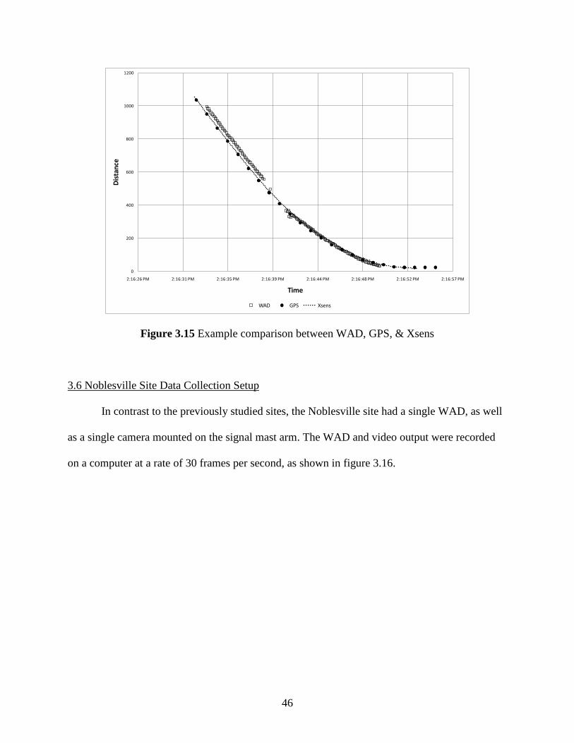
46
Figure 3.15 Example comparison between WAD, GPS, & Xsens
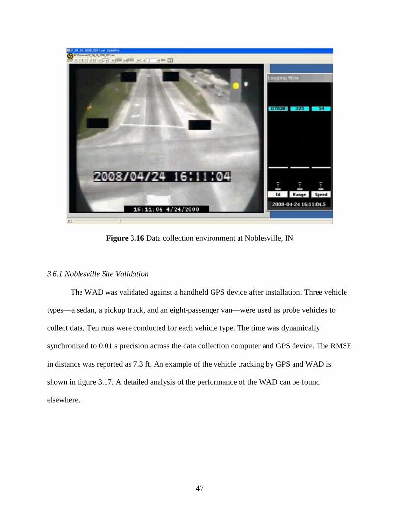
3.6 Noblesville Site Data Collection Setup
In contrast to the previously studied sites, the Noblesville site had a single WAD, as well
as a single camera mounted on the signal mast arm. The WAD and video output were recorded
on a computer at a rate of 30 frames per second, as shown in figure 3.16.
0
200
400
600
800
1000
1200
2:16:26 PM 2:16:31 PM 2:16:35 PM 2:16:39 PM 2:16:44 PM 2:16:48 PM 2:16:52 PM 2:16:57 PM
Dis
tan
ce
Time
WAD GPS Xsens
47
Figure 3.16 Data collection environment at Noblesville, IN
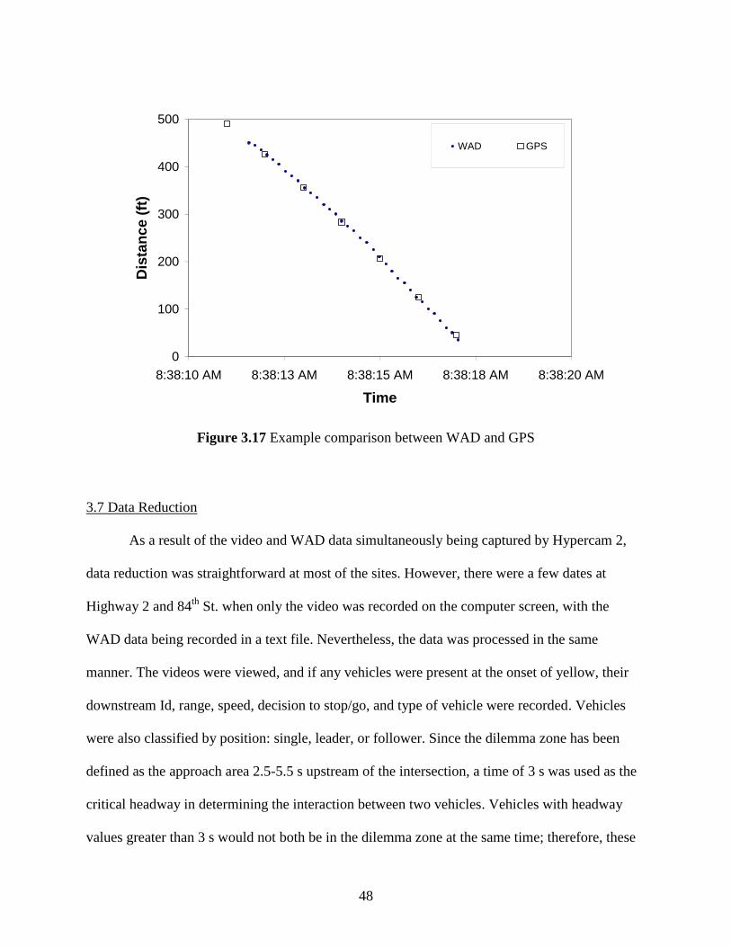
3.6.1 Noblesville Site Validation
The WAD was validated against a handheld GPS device after installation. Three vehicle
types—a sedan, a pickup truck, and an eight-passenger van—were used as probe vehicles to
collect data. Ten runs were conducted for each vehicle type. The time was dynamically
synchronized to 0.01 s precision across the data collection computer and GPS device. The RMSE
in distance was reported as 7.3 ft. An example of the vehicle tracking by GPS and WAD is
shown in figure 3.17. A detailed analysis of the performance of the WAD can be found
elsewhere.
48
Figure 3.17 Example comparison between WAD and GPS
3.7 Data Reduction
As a result of the video and WAD data simultaneously being captured by Hypercam 2,
data reduction was straightforward at most of the sites. However, there were a few dates at
Highway 2 and 84th
St. when only the video was recorded on the computer screen, with the
WAD data being recorded in a text file. Nevertheless, the data was processed in the same
manner. The videos were viewed, and if any vehicles were present at the onset of yellow, their
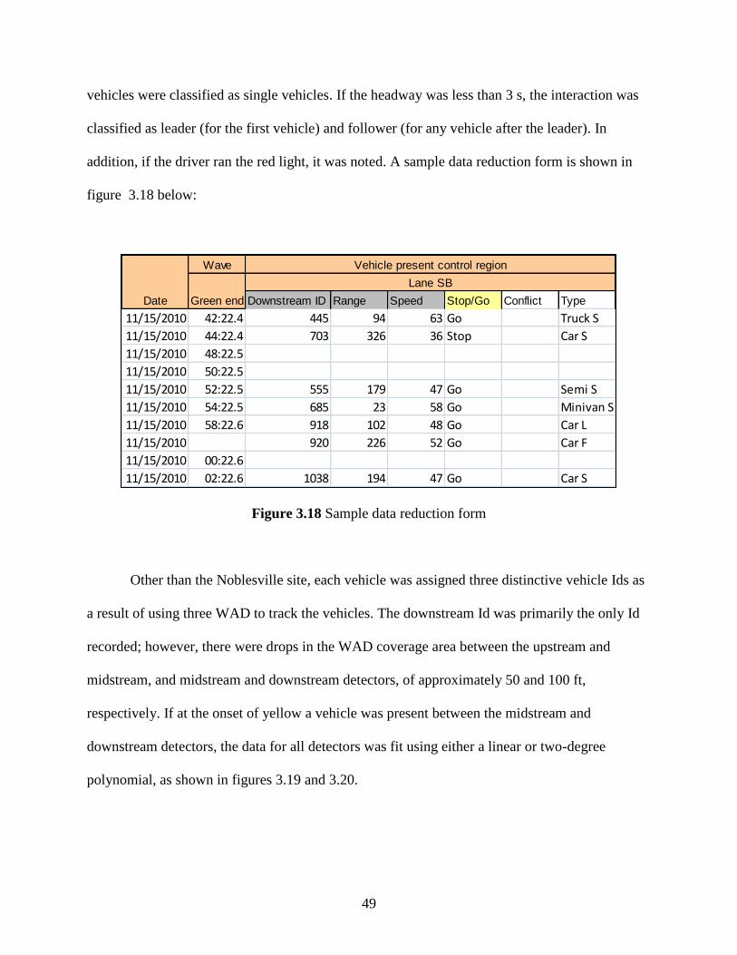
downstream Id, range, speed, decision to stop/go, and type of vehicle were recorded. Vehicles
were also classified by position: single, leader, or follower. Since the dilemma zone has been
defined as the approach area 2.5-5.5 s upstream of the intersection, a time of 3 s was used as the
critical headway in determining the interaction between two vehicles. Vehicles with headway
values greater than 3 s would not both be in the dilemma zone at the same time; therefore, these
0
100
200
300
400
500
8:38:10 AM 8:38:13 AM 8:38:15 AM 8:38:18 AM 8:38:20 AM
Time
Dis
tan
ce (
ft)
WAD GPS
49
vehicles were classified as single vehicles. If the headway was less than 3 s, the interaction was
classified as leader (for the first vehicle) and follower (for any vehicle after the leader). In
addition, if the driver ran the red light, it was noted. A sample data reduction form is shown in
figure 3.18 below:
Figure 3.18 Sample data reduction form
Other than the Noblesville site, each vehicle was assigned three distinctive vehicle Ids as
a result of using three WAD to track the vehicles. The downstream Id was primarily the only Id
recorded; however, there were drops in the WAD coverage area between the upstream and
midstream, and midstream and downstream detectors, of approximately 50 and 100 ft,
respectively. If at the onset of yellow a vehicle was present between the midstream and
downstream detectors, the data for all detectors was fit using either a linear or two-degree
polynomial, as shown in figures 3.19 and 3.20.
Wave
Downstream ID Range Speed Stop/Go Conflict Type
11/15/2010 42:22.4 445 94 63 Go Truck S
11/15/2010 44:22.4 703 326 36 Stop Car S
11/15/2010 48:22.5
11/15/2010 50:22.5
11/15/2010 52:22.5 555 179 47 Go Semi S
11/15/2010 54:22.5 685 23 58 Go Minivan S
11/15/2010 58:22.6 918 102 48 Go Car L
11/15/2010 920 226 52 Go Car F
11/15/2010 00:22.6
11/15/2010 02:22.6 1038 194 47 Go Car S
Date
Vehicle present control region
Green end
Lane SB
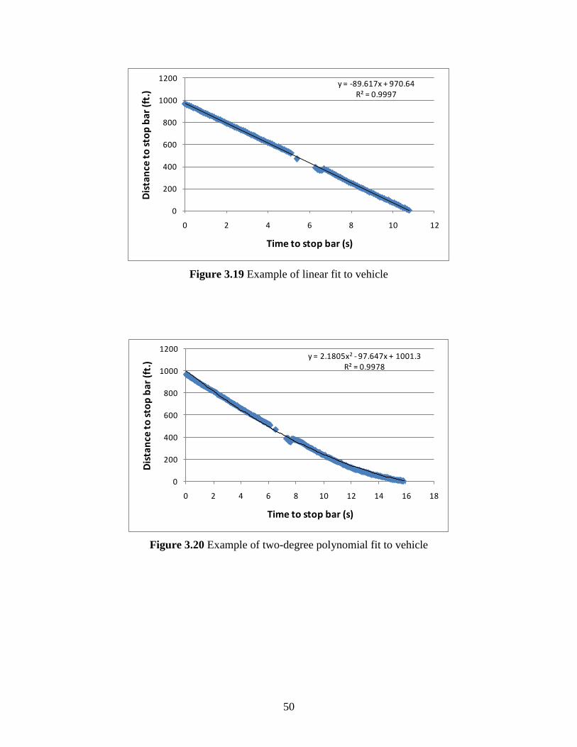
50
Figure 3.19 Example of linear fit to vehicle
Figure 3.20 Example of two-degree polynomial fit to vehicle
y = -89.617x + 970.64R² = 0.9997
0
200
400
600
800
1000
1200
0 2 4 6 8 10 12
Dis
tan
ce t
o s
top
bar
(ft.
)
Time to stop bar (s)
y = 2.1805x2 - 97.647x + 1001.3R² = 0.9978
0
200
400
600
800
1000
1200
0 2 4 6 8 10 12 14 16 18
Dis
tan
ce t
o s
top
ba
r (f
t.)
Time to stop bar (s)
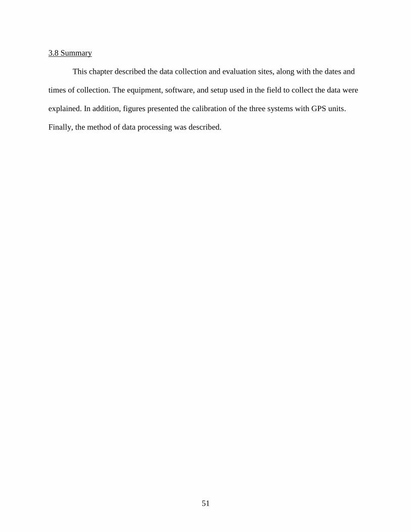
51
3.8 Summary
This chapter described the data collection and evaluation sites, along with the dates and
times of collection. The equipment, software, and setup used in the field to collect the data were
explained. In addition, figures presented the calibration of the three systems with GPS units.
Finally, the method of data processing was described.
52
Chapter 4 Role of Information on Dilemma Hazard Function
4.1Theory Underlying Driver Decision Making
Driver behavior at the onset of yellow is essentially a binary choice process in which the
driver chooses from two possible courses of action: stop or go (Sheffi and Mahmassani 1981).
Let Tp be the time to the stop bar perceived by a driver randomly selected from the population; as
a result of the variance in driver behavior based on several independent factors such as
perception of the distance from the stop bar, perception reaction time, perception of the yellow
interval based on past experience, etc., Tp can be modeled as a normally distributed random
variable, as shown below in equation 4.1.
reqp TT
(4.1)
where,
Treq is the required time to stop bar;
: is a random variable which is assumed to be normally distributed.
Similar analyses have been performed using the perceived and required time to the stop
bar and the perceived and required acceleration (Sheffi and Mahmassani 1981; Sharma et al.
2010). If the perceived time to the stop bar is less than a certain critical time threshold, the driver
decides to stop; if the time is greater than this threshold, the driver decides to go. The critical
time threshold for a given site can be estimated by the probability of stopping curves. At the
point at which the required time to stop bar is equal to the critical time threshold, the probability
of stopping is 0.5. Under ideal weather conditions, and assuming the vehicles are passenger
53
vehicles, the critical threshold should be equal to the designed yellow time; this implies that if
the perceived time to the stop bar is greater than the provided yellow time, the driver will decide
to stop, whereas if the perceived time to the stop bar is less than the provided yellow time, the
driver will decide to go. It should be noted that error in driver perception of yellow time can be
added to driver perception of travel time error if we assume the yellow duration error to be
normally distributed as well.
Two other critical thresholds can be calculated for a driver approaching the intersection at
the onset of yellow: the distance requiring severe deceleration and the distance at which a driver
would accelerate heavily or run the red light. The following calculations were performed as
examples of the acceleration and deceleration threshold, based on 85th
percentile acceleration and
deceleration values derived from Sharma (2008). The distance at which a vehicle cannot proceed
through the intersection without heavily accelerating or RLR is calculated by:
(4.2)
where,
speed is the speed of the vehicle at the onset of yellow (ft/s);
yellow is the length of yellow (s);
a is the 85th
percentile acceleration, 3.19 ft/s2 (Sharma 2008);
PRT perception reaction time of 1 s.
For a speed of 80.667 ft/s (55 mph) and a yellow length of 4.9 s, the critical acceleration
distance equals 420 ft. This distance will be referred to as the maximum passing distance for the
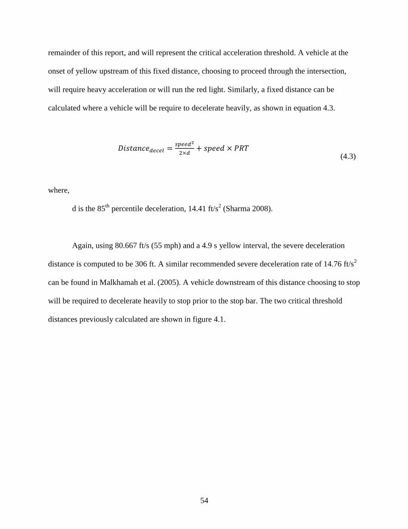
54
remainder of this report, and will represent the critical acceleration threshold. A vehicle at the
onset of yellow upstream of this fixed distance, choosing to proceed through the intersection,
will require heavy acceleration or will run the red light. Similarly, a fixed distance can be
calculated where a vehicle will be require to decelerate heavily, as shown in equation 4.3.
(4.3)
where,
d is the 85th
percentile deceleration, 14.41 ft/s2 (Sharma 2008).
Again, using 80.667 ft/s (55 mph) and a 4.9 s yellow interval, the severe deceleration
distance is computed to be 306 ft. A similar recommended severe deceleration rate of 14.76 ft/s2
can be found in Malkhamah et al. (2005). A vehicle downstream of this distance choosing to stop
will be required to decelerate heavily to stop prior to the stop bar. The two critical threshold
distances previously calculated are shown in figure 4.1.
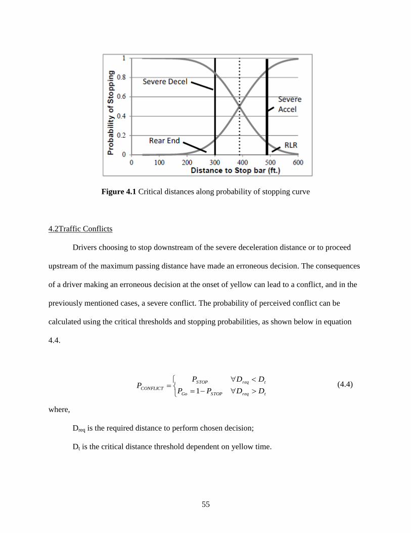
55
Figure 4.1 Critical distances along probability of stopping curve
4.2Traffic Conflicts
Drivers choosing to stop downstream of the severe deceleration distance or to proceed
upstream of the maximum passing distance have made an erroneous decision. The consequences
of a driver making an erroneous decision at the onset of yellow can lead to a conflict, and in the
previously mentioned cases, a severe conflict. The probability of perceived conflict can be
calculated using the critical thresholds and stopping probabilities, as shown below in equation
4.4.
(4.4)
where,
Dreq is the required distance to perform chosen decision;
Dt is the critical distance threshold dependent on yellow time.
treqSTOPGo
treqSTOP
CONFLICT DDPP
DDPP
1
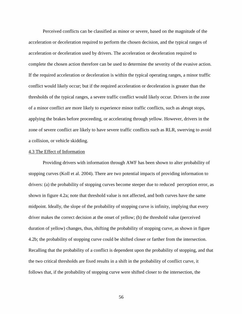
56
Perceived conflicts can be classified as minor or severe, based on the magnitude of the
acceleration or deceleration required to perform the chosen decision, and the typical ranges of
acceleration or deceleration used by drivers. The acceleration or deceleration required to
complete the chosen action therefore can be used to determine the severity of the evasive action.
If the required acceleration or deceleration is within the typical operating ranges, a minor traffic
conflict would likely occur; but if the required acceleration or deceleration is greater than the
thresholds of the typical ranges, a severe traffic conflict would likely occur. Drivers in the zone
of a minor conflict are more likely to experience minor traffic conflicts, such as abrupt stops,
applying the brakes before proceeding, or accelerating through yellow. However, drivers in the
zone of severe conflict are likely to have severe traffic conflicts such as RLR, swerving to avoid
a collision, or vehicle skidding.
4.3 The Effect of Information
Providing drivers with information through AWF has been shown to alter probability of
stopping curves (Koll et al. 2004). There are two potential impacts of providing information to
drivers: (a) the probability of stopping curves become steeper due to reduced perception error, as
shown in figure 4.2a; note that threshold value is not affected, and both curves have the same
midpoint. Ideally, the slope of the probability of stopping curve is infinity, implying that every
driver makes the correct decision at the onset of yellow; (b) the threshold value (perceived
duration of yellow) changes, thus, shifting the probability of stopping curve, as shown in figure
4.2b; the probability of stopping curve could be shifted closer or farther from the intersection.
Recalling that the probability of a conflict is dependent upon the probability of stopping, and that
the two critical thresholds are fixed results in a shift in the probability of conflict curve, it
follows that, if the probability of stopping curve were shifted closer to the intersection, the
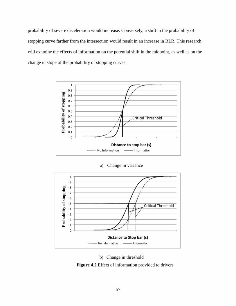
57
probability of severe deceleration would increase. Conversely, a shift in the probability of
stopping curve farther from the intersection would result in an increase in RLR. This research
will examine the effects of information on the potential shift in the midpoint, as well as on the
change in slope of the probability of stopping curves.
a) Change in variance
b) Change in threshold
Figure 4.2 Effect of information provided to drivers
0
0.1
0.2
0.3
0.4
0.5
0.6
0.7
0.8
0.9
1
Proba bility of Stoppi ng
Distance to stop bar (s)
No Information Information
Critical Threshold
Pro
bab
ilit
y o
f st
op
pin
g
0
0.1
0.2
0.3
0.4
0.5
0.6
0.7
0.8
0.9
1
Proba bility of Stoppi ng
Distance to Stop bar (s)
No Information Information
Critical Threshold
Pro
bab
ilit
y o
f st
op
pin
g
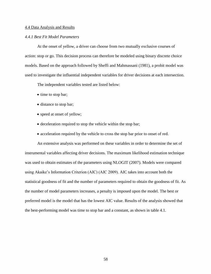
58
4.4 Data Analysis and Results
4.4.1 Best Fit Model Parameters
At the onset of yellow, a driver can choose from two mutually exclusive courses of
action: stop or go. This decision process can therefore be modeled using binary discrete choice
models. Based on the approach followed by Sheffi and Mahmassani (1981), a probit model was
used to investigate the influential independent variables for driver decisions at each intersection.
The independent variables tested are listed below:
time to stop bar;
distance to stop bar;
speed at onset of yellow;
deceleration required to stop the vehicle within the stop bar;
acceleration required by the vehicle to cross the stop bar prior to onset of red.
An extensive analysis was performed on these variables in order to determine the set of
instrumental variables affecting driver decisions. The maximum likelihood estimation technique
was used to obtain estimates of the parameters using NLOGIT (2007). Models were compared
using Akaike’s Information Criterion (AIC) (AIC 2009). AIC takes into account both the
statistical goodness of fit and the number of parameters required to obtain the goodness of fit. As
the number of model parameters increases, a penalty is imposed upon the model. The best or
preferred model is the model that has the lowest AIC value. Results of the analysis showed that
the best-performing model was time to stop bar and a constant, as shown in table 4.1.
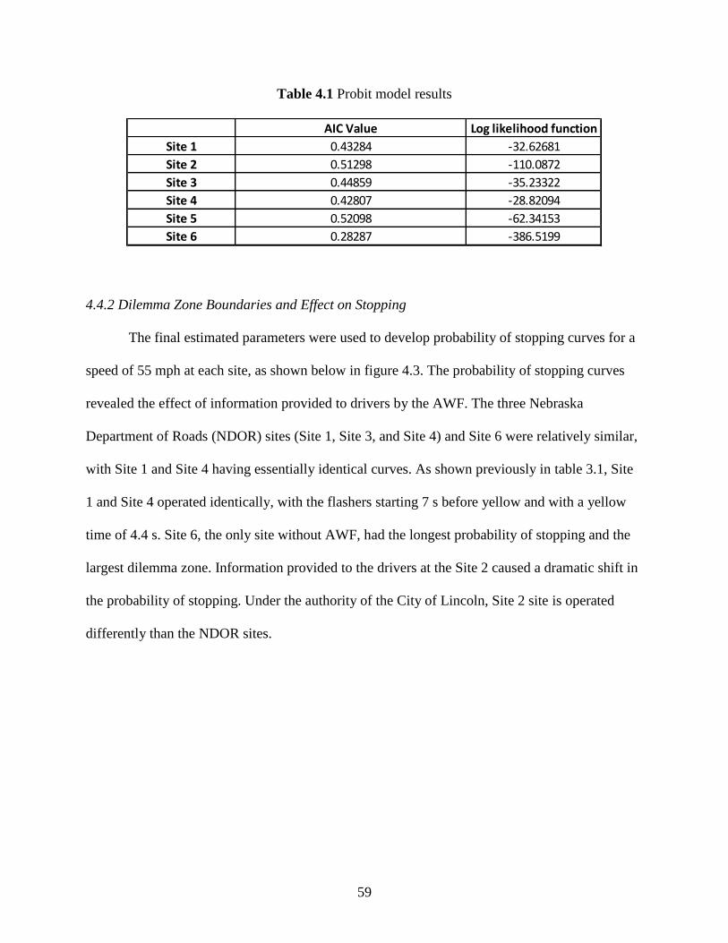
59
Table 4.1 Probit model results
4.4.2 Dilemma Zone Boundaries and Effect on Stopping
The final estimated parameters were used to develop probability of stopping curves for a
speed of 55 mph at each site, as shown below in figure 4.3. The probability of stopping curves
revealed the effect of information provided to drivers by the AWF. The three Nebraska
Department of Roads (NDOR) sites (Site 1, Site 3, and Site 4) and Site 6 were relatively similar,
with Site 1 and Site 4 having essentially identical curves. As shown previously in table 3.1, Site
1 and Site 4 operated identically, with the flashers starting 7 s before yellow and with a yellow
time of 4.4 s. Site 6, the only site without AWF, had the longest probability of stopping and the
largest dilemma zone. Information provided to the drivers at the Site 2 caused a dramatic shift in
the probability of stopping. Under the authority of the City of Lincoln, Site 2 site is operated
differently than the NDOR sites.
AIC Value Log likelihood function
Site 1 0.43284 -32.62681
Site 2 0.51298 -110.0872
Site 3 0.44859 -35.23322
Site 4 0.42807 -28.82094
Site 5 0.52098 -62.34153
Site 6 0.28287 -386.5199
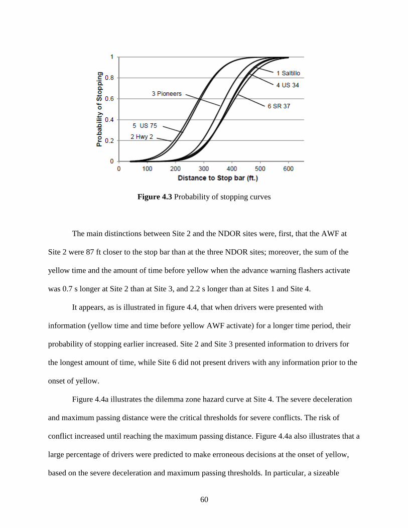
60
Figure 4.3 Probability of stopping curves
The main distinctions between Site 2 and the NDOR sites were, first, that the AWF at
Site 2 were 87 ft closer to the stop bar than at the three NDOR sites; moreover, the sum of the
yellow time and the amount of time before yellow when the advance warning flashers activate
was 0.7 s longer at Site 2 than at Site 3, and 2.2 s longer than at Sites 1 and Site 4.
It appears, as is illustrated in figure 4.4, that when drivers were presented with
information (yellow time and time before yellow AWF activate) for a longer time period, their
probability of stopping earlier increased. Site 2 and Site 3 presented information to drivers for
the longest amount of time, while Site 6 did not present drivers with any information prior to the
onset of yellow.
Figure 4.4a illustrates the dilemma zone hazard curve at Site 4. The severe deceleration
and maximum passing distance were the critical thresholds for severe conflicts. The risk of
conflict increased until reaching the maximum passing distance. Figure 4.4a also illustrates that a
large percentage of drivers were predicted to make erroneous decisions at the onset of yellow,
based on the severe deceleration and maximum passing thresholds. In particular, a sizeable
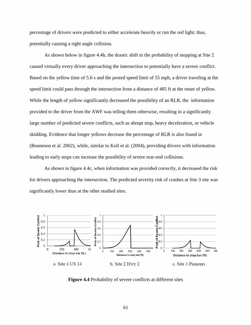
61
percentage of drivers were predicted to either accelerate heavily or run the red light; thus,
potentially causing a right angle collision.
As shown below in figure 4.4b, the drastic shift in the probability of stopping at Site 2
caused virtually every driver approaching the intersection to potentially have a severe conflict.
Based on the yellow time of 5.6 s and the posted speed limit of 55 mph, a driver traveling at the
speed limit could pass through the intersection from a distance of 485 ft at the onset of yellow.
While the length of yellow significantly decreased the possibility of an RLR, the information
provided to the driver from the AWF was telling them otherwise, resulting in a significantly
large number of predicted severe conflicts, such as abrupt stop, heavy deceleration, or vehicle
skidding. Evidence that longer yellows decrease the percentage of RLR is also found in
(Bonneson et al. 2002), while, similar to Koll et al. (2004), providing drivers with information
leading to early stops can increase the possibility of severe rear-end collisions.
As shown in figure 4.4c, when information was provided correctly, it decreased the risk
for drivers approaching the intersection. The predicted severity risk of crashes at Site 3 site was
significantly lower than at the other studied sites.
Figure 4.4 Probability of severe conflicts at different sites
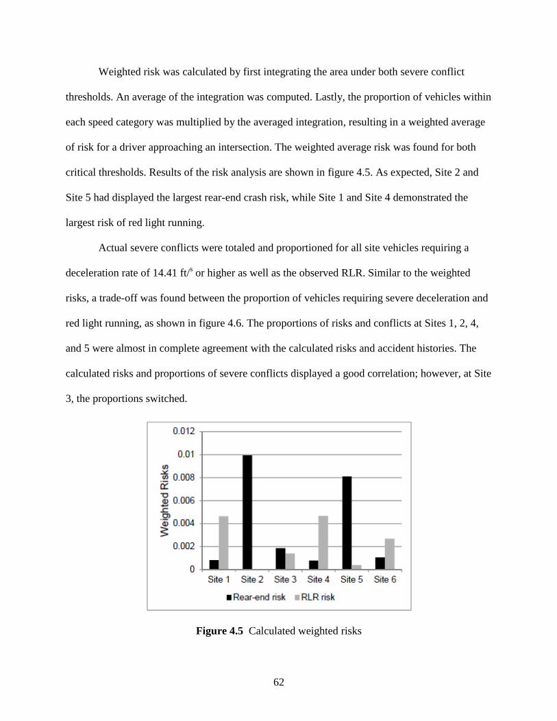
62
Weighted risk was calculated by first integrating the area under both severe conflict
thresholds. An average of the integration was computed. Lastly, the proportion of vehicles within
each speed category was multiplied by the averaged integration, resulting in a weighted average
of risk for a driver approaching an intersection. The weighted average risk was found for both
critical thresholds. Results of the risk analysis are shown in figure 4.5. As expected, Site 2 and
Site 5 had displayed the largest rear-end crash risk, while Site 1 and Site 4 demonstrated the
largest risk of red light running.
Actual severe conflicts were totaled and proportioned for all site vehicles requiring a
deceleration rate of 14.41 ft/s or higher as well as the observed RLR. Similar to the weighted
risks, a trade-off was found between the proportion of vehicles requiring severe deceleration and
red light running, as shown in figure 4.6. The proportions of risks and conflicts at Sites 1, 2, 4,
and 5 were almost in complete agreement with the calculated risks and accident histories. The
calculated risks and proportions of severe conflicts displayed a good correlation; however, at Site
3, the proportions switched.
Figure 4.5 Calculated weighted risks
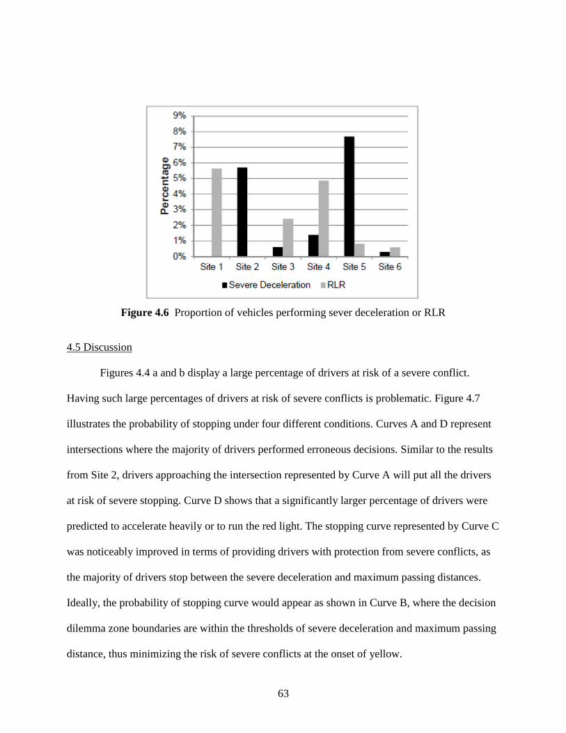
63
Figure 4.6 Proportion of vehicles performing sever deceleration or RLR
4.5 Discussion
Figures 4.4 a and b display a large percentage of drivers at risk of a severe conflict.
Having such large percentages of drivers at risk of severe conflicts is problematic. Figure 4.7
illustrates the probability of stopping under four different conditions. Curves A and D represent
intersections where the majority of drivers performed erroneous decisions. Similar to the results
from Site 2, drivers approaching the intersection represented by Curve A will put all the drivers
at risk of severe stopping. Curve D shows that a significantly larger percentage of drivers were
predicted to accelerate heavily or to run the red light. The stopping curve represented by Curve C
was noticeably improved in terms of providing drivers with protection from severe conflicts, as
the majority of drivers stop between the severe deceleration and maximum passing distances.
Ideally, the probability of stopping curve would appear as shown in Curve B, where the decision
dilemma zone boundaries are within the thresholds of severe deceleration and maximum passing
distance, thus minimizing the risk of severe conflicts at the onset of yellow.
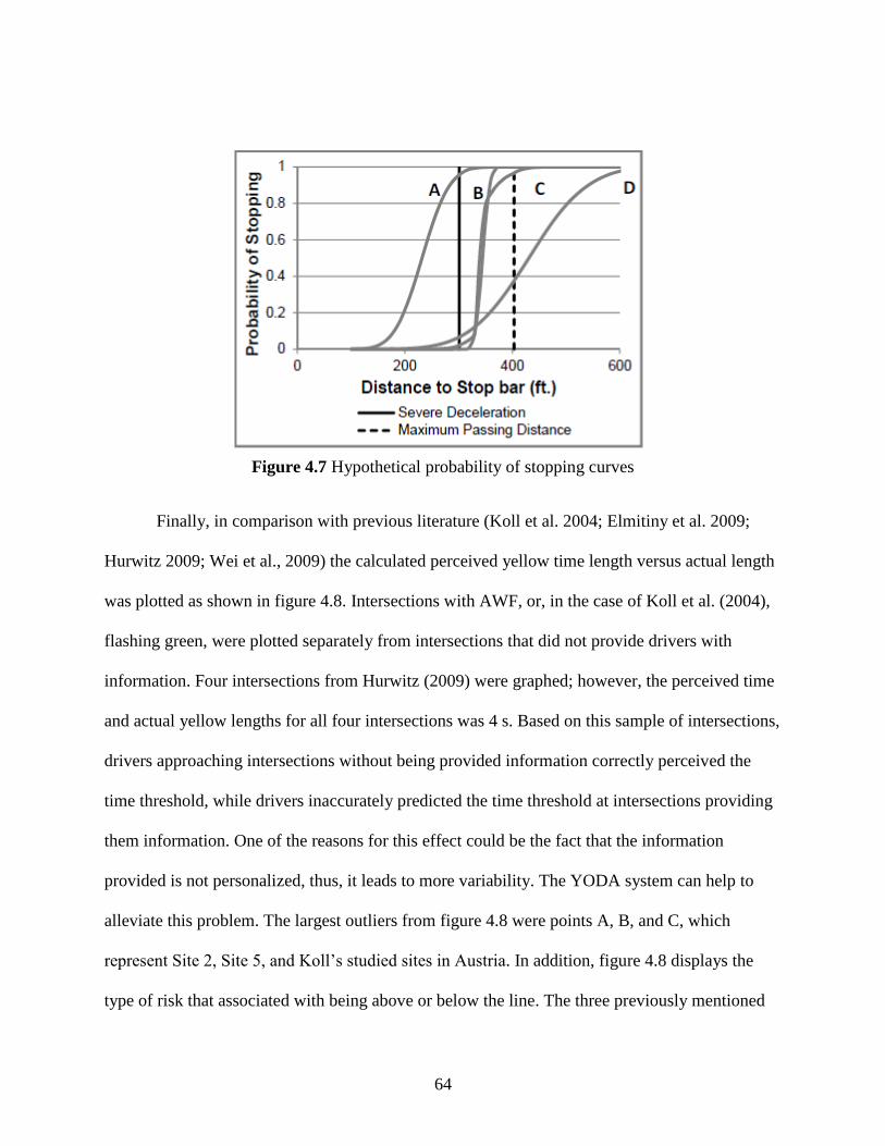
64
Figure 4.7 Hypothetical probability of stopping curves
Finally, in comparison with previous literature (Koll et al. 2004; Elmitiny et al. 2009;
Hurwitz 2009; Wei et al., 2009) the calculated perceived yellow time length versus actual length
was plotted as shown in figure 4.8. Intersections with AWF, or, in the case of Koll et al. (2004),
flashing green, were plotted separately from intersections that did not provide drivers with
information. Four intersections from Hurwitz (2009) were graphed; however, the perceived time
and actual yellow lengths for all four intersections was 4 s. Based on this sample of intersections,
drivers approaching intersections without being provided information correctly perceived the
time threshold, while drivers inaccurately predicted the time threshold at intersections providing
them information. One of the reasons for this effect could be the fact that the information
provided is not personalized, thus, it leads to more variability. The YODA system can help to
alleviate this problem. The largest outliers from figure 4.8 were points A, B, and C, which
represent Site 2, Site 5, and Koll’s studied sites in Austria. In addition, figure 4.8 displays the
type of risk that associated with being above or below the line. The three previously mentioned
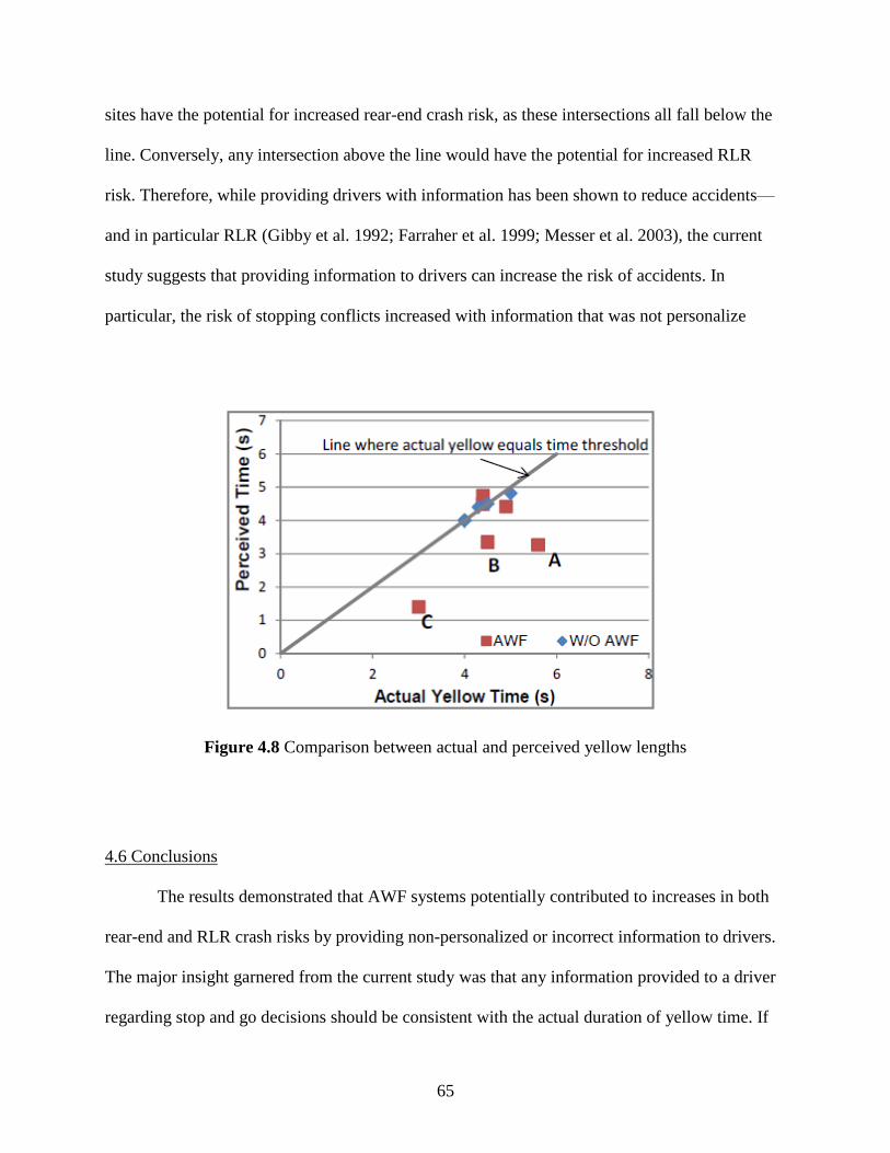
65
sites have the potential for increased rear-end crash risk, as these intersections all fall below the
line. Conversely, any intersection above the line would have the potential for increased RLR
risk. Therefore, while providing drivers with information has been shown to reduce accidents—
and in particular RLR (Gibby et al. 1992; Farraher et al. 1999; Messer et al. 2003), the current
study suggests that providing information to drivers can increase the risk of accidents. In
particular, the risk of stopping conflicts increased with information that was not personalize
Figure 4.8 Comparison between actual and perceived yellow lengths
4.6 Conclusions
The results demonstrated that AWF systems potentially contributed to increases in both
rear-end and RLR crash risks by providing non-personalized or incorrect information to drivers.
The major insight garnered from the current study was that any information provided to a driver
regarding stop and go decisions should be consistent with the actual duration of yellow time. If
66
the yellow time is longer that as implied by the AWF and the driver is incorrectly signaled to
stop, the outcome is more confusion, resulting in higher-risk intersections. It should also be
noted that when no information was provided, the critical time threshold for stopping was very
close to the actual yellow duration. This shows that drivers usually were likely to stop when the
time to the stop bar was greater than the yellow time, and were likely to go when the time to stop
bar was less than the yellow duration. The next chapter presents the details of a prototype YODA
system, developed for this study, which utilizes this concept to inform stop and go decisions; the
YODA system provides personalized information to the driver based on the time to the stop bar
and the remaining yellow time.
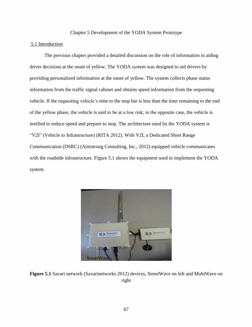
67
Chapter 5 Development of the YODA System Prototype
5.1 Introduction
The previous chapter provided a detailed discussion on the role of information in aiding
driver decisions at the onset of yellow. The YODA system was designed to aid drivers by
providing personalized information at the onset of yellow. The system collects phase status
information from the traffic signal cabinet and obtains speed information from the requesting
vehicle. If the requesting vehicle’s time to the stop bar is less than the time remaining to the end
of the yellow phase, the vehicle is said to be at a low risk; in the opposite case, the vehicle is
notified to reduce speed and prepare to stop. The architecture used by the YODA system is
“V2I” (Vehicle to Infrastructure) (RITA 2012). With V2I, a Dedicated Short Range
Communication (DSRC) (Armstrong Consulting, Inc., 2012) equipped vehicle communicates
with the roadside infrastructure. Figure 5.1 shows the equipment used to implement the YODA
system.
Figure 5.1 Savari network (Savarinetworks 2012) devices, StreetWave on left and MobiWave on
right
StreetWave
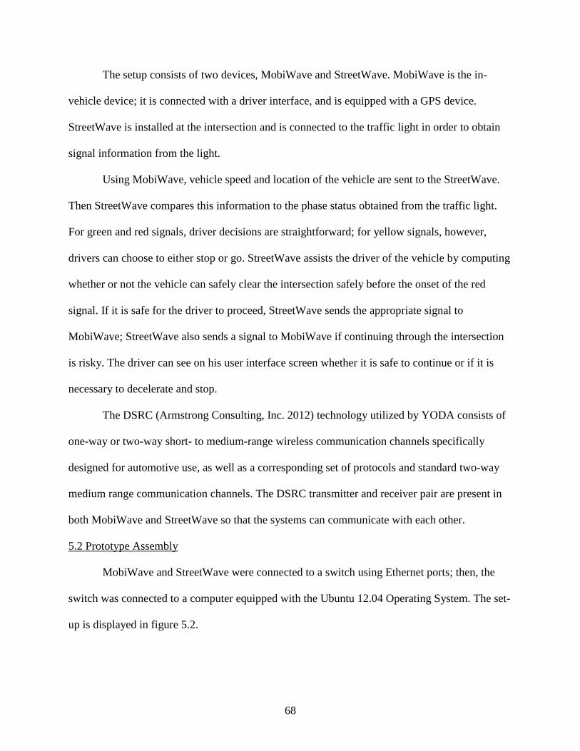
68
The setup consists of two devices, MobiWave and StreetWave. MobiWave is the in-
vehicle device; it is connected with a driver interface, and is equipped with a GPS device.
StreetWave is installed at the intersection and is connected to the traffic light in order to obtain
signal information from the light.
Using MobiWave, vehicle speed and location of the vehicle are sent to the StreetWave.
Then StreetWave compares this information to the phase status obtained from the traffic light.
For green and red signals, driver decisions are straightforward; for yellow signals, however,
drivers can choose to either stop or go. StreetWave assists the driver of the vehicle by computing
whether or not the vehicle can safely clear the intersection safely before the onset of the red
signal. If it is safe for the driver to proceed, StreetWave sends the appropriate signal to
MobiWave; StreetWave also sends a signal to MobiWave if continuing through the intersection
is risky. The driver can see on his user interface screen whether it is safe to continue or if it is
necessary to decelerate and stop.
The DSRC (Armstrong Consulting, Inc. 2012) technology utilized by YODA consists of
one-way or two-way short- to medium-range wireless communication channels specifically
designed for automotive use, as well as a corresponding set of protocols and standard two-way
medium range communication channels. The DSRC transmitter and receiver pair are present in
both MobiWave and StreetWave so that the systems can communicate with each other.
5.2 Prototype Assembly
MobiWave and StreetWave were connected to a switch using Ethernet ports; then, the
switch was connected to a computer equipped with the Ubuntu 12.04 Operating System. The set-
up is displayed in figure 5.2.

69
Figure 5.2 Connection set-up for development purposes
The following steps were taken to successfully install our software packages to
MobiWave and StreetWave. Please note that throughout this part of the documents all codes are
presented in italics.
Step 1 consisted of connecting the development machine to MobiWave/Street Wave. The
terminal screen on Ubuntu was displayed by holding Ctrl + Tab and pressing T. Repeating his
sequence three consecutive times resulted in opening three different terminals, one for the
developing computer, one for MobiWave, and one for StreetWave.
In the terminal opened for MobiWave, entering the command: ssh [email protected]
resulted in connecting to the device operating system. First, the password gems was entered;
following password entry, the operating system was displayed on the terminal assigned to
MobiWave, as shown in figure 5.3:
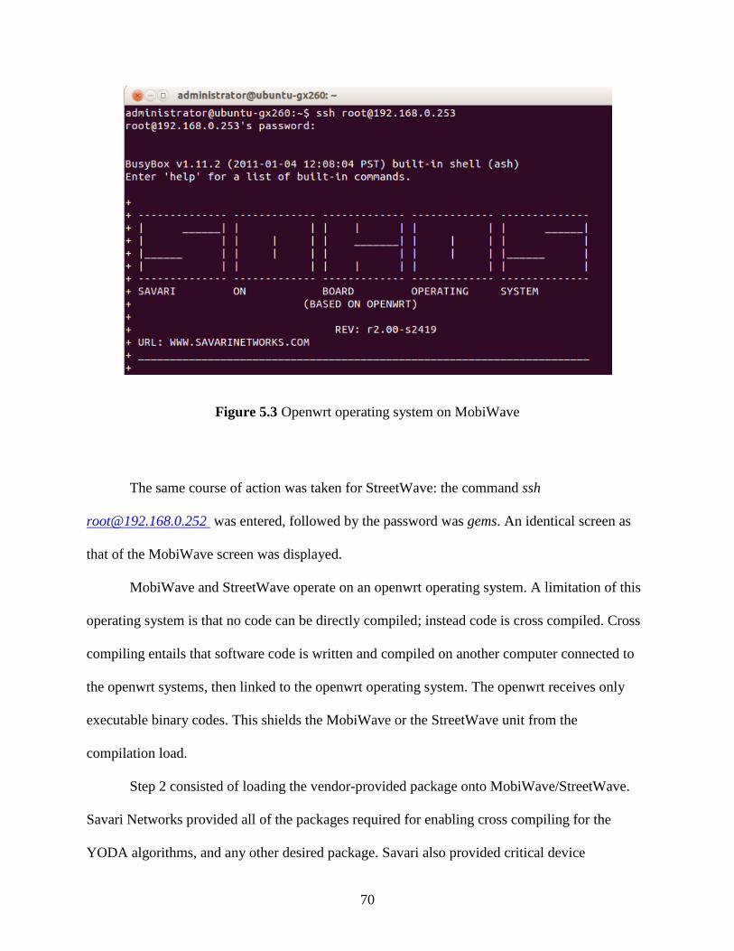
70
Figure 5.3 Openwrt operating system on MobiWave
The same course of action was taken for StreetWave: the command ssh
[email protected] was entered, followed by the password was gems. An identical screen as
that of the MobiWave screen was displayed.
MobiWave and StreetWave operate on an openwrt operating system. A limitation of this
operating system is that no code can be directly compiled; instead code is cross compiled. Cross
compiling entails that software code is written and compiled on another computer connected to
the openwrt systems, then linked to the openwrt operating system. The openwrt receives only
executable binary codes. This shields the MobiWave or the StreetWave unit from the
compilation load.
Step 2 consisted of loading the vendor-provided package onto MobiWave/StreetWave.
Savari Networks provided all of the packages required for enabling cross compiling for the
YODA algorithms, and any other desired package. Savari also provided critical device
71
specifications for hardware usage. Since the packages were in compressed format, after the
packages were copied onto the development computer they needed to be extracted using the code
listed below. The first step, using the terminal specified for the developing computer, was to use
cd command to arrive at the directory upon which the packages were copied, and enter:
%tar -jxvf SOBOS-X-SDK-x86-for-Linux-i686(correct file name).tar.bz2 (5.1)
Some sample codes were provided by the vendor. In order to enable cross compiling, it
was necessary to link the file path where the package intended to be placed on
MobiWave/StreetWave, then convert them to binary. First it was necessary to link the simple,
vendor- provided helloworld package because it generated the correct folder structure, which
would be of use in any other desired package. Again using cd command prompted the SOBOS-X-
SDK-x86-for-Linux-i686 folder, which is referred as SOBOS in the remainder of this report. The
code required for linking a package was as follows:
% ln -s ../../sdk-sample-apps/helloworld (5.2)
where,
ln is a Unix command for linking files or directories to each other.
In the SOBOS folder, the command make V=99. Make V=99 was entered when
compiling system output was desired in verbose mode. Verbose mode, by definition, is a mode in
which varying levels of status messages are displayed during processing. This command resulted
72
in the creation of a new file in the folder packages—helloworld.ipk—which was ready to be
transferred to the openwrt operating system.
Step 3 involved copying the package on MobiWAVE. On the development computer
terminal, using the command below or any other command that used CD , the folder packages
located in the folder bin were accessed:
cd SOBOS-SDK-x86-for-Linux-i686(correct file name)/bin/packages/i386 (5.3)
There, the package was copied on MobiWave using the instruction below:
scp helloworld.ipk [email protected]:/tmp (5.4)
scp or, secure copy, copies files between hosts on a network. It uses ssh protocol, implying that
the data transferred is encrypted and authentication is needed to copy the data. On the terminal
that was connected to MobiWave, researchers typed in: cd /tmp , which opened the tmp folder.
Typing the instruction below installed the code on the MobiWave.
opkg1 install ./helloworld*.ipk (5.5)
Opkg is a lightweight package management system based on Ipkg, used in older versions
of openwrt. It can install, update, and remove individual software packages, resolve
dependencies between packages, and so on. After this command, typing
1 In the guide it was written ‘ipkg,’ which will result in an error. In the newer versions of openwrt (such as used
here), the correct command is ‘opkg.’
73
/usr/local/bin/helloworld loaded the application, and resulted simply in MobiWave saying: Hello
World!
The helloworld.ipk file on StreetWave can also be copied using the terminal specified to
it to obtain similar results.
Step 4 entailed installing specific packages on the MobiWave/StreetWave. The file
structure is described in next section in detail. It should be noted that our package contained a
file named its_trafficlight.c. Once opened, the screen read:
#define CARz. Notably, this differs from “CAR.” Anything other than CAR was compiled
for StreetWave. If CARz was changed to CAR, it was compiled for MobiWave.
Steps taken here were almost completely identical to the vendor-provided package
helloworld. The name of the package designed by the researchers was its_trafficlight. All the
steps were taken exactly as mentioned above, but, instead of helloworld, the term its_trafficlight
was used. However once the package its_trafficlight.ipk was generated for StreetWave and
copied, the file its_trafficlight.c was opened and CARz was changed to CAR, at which point
another its_trafficlight.ipk was generated and copied on MobiWave.
Step 5 involved understand the displays on the terminals. As a result of connecting to the
terminals of MobiWave and StreetWave, the results obtained while running the code can be seen
below. Here 3 scenarios may occur:
A) The MobiWave is not getting any data from StreetWave, and vice versa:
In this case the devices do not communicate with each other. Figure 5.4 briefly
describes how each operates in this case:
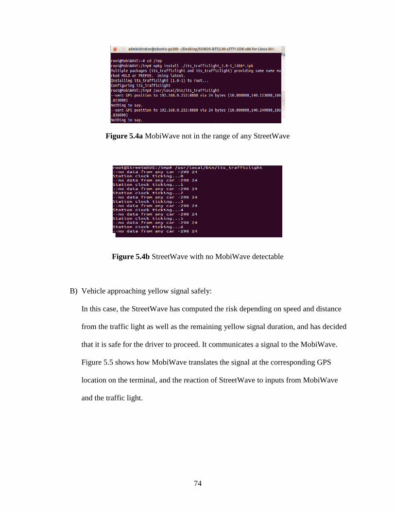
74
Figure 5.4a MobiWave not in the range of any StreetWave
Figure 5.4b StreetWave with no MobiWave detectable
B) Vehicle approaching yellow signal safely:
In this case, the StreetWave has computed the risk depending on speed and distance
from the traffic light as well as the remaining yellow signal duration, and has decided
that it is safe for the driver to proceed. It communicates a signal to the MobiWave.
Figure 5.5 shows how MobiWave translates the signal at the corresponding GPS
location on the terminal, and the reaction of StreetWave to inputs from MobiWave
and the traffic light.
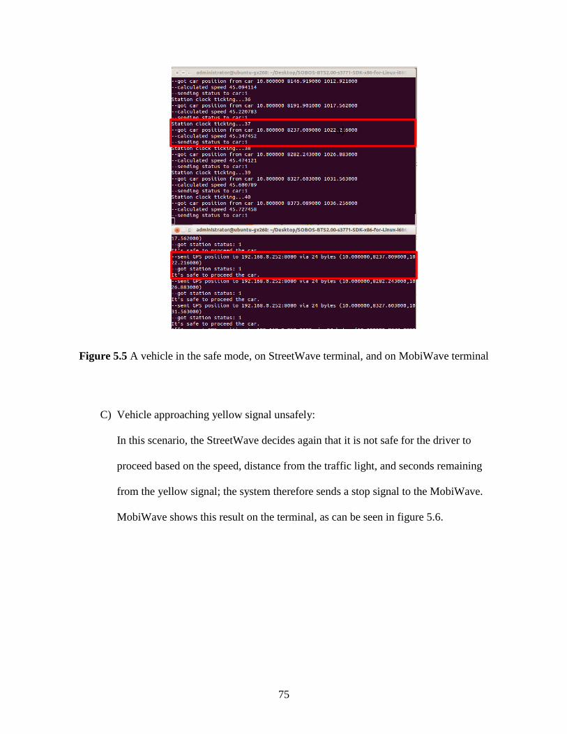
75
Figure 5.5 A vehicle in the safe mode, on StreetWave terminal, and on MobiWave terminal
C) Vehicle approaching yellow signal unsafely:
In this scenario, the StreetWave decides again that it is not safe for the driver to
proceed based on the speed, distance from the traffic light, and seconds remaining
from the yellow signal; the system therefore sends a stop signal to the MobiWave.
MobiWave shows this result on the terminal, as can be seen in figure 5.6.
a)
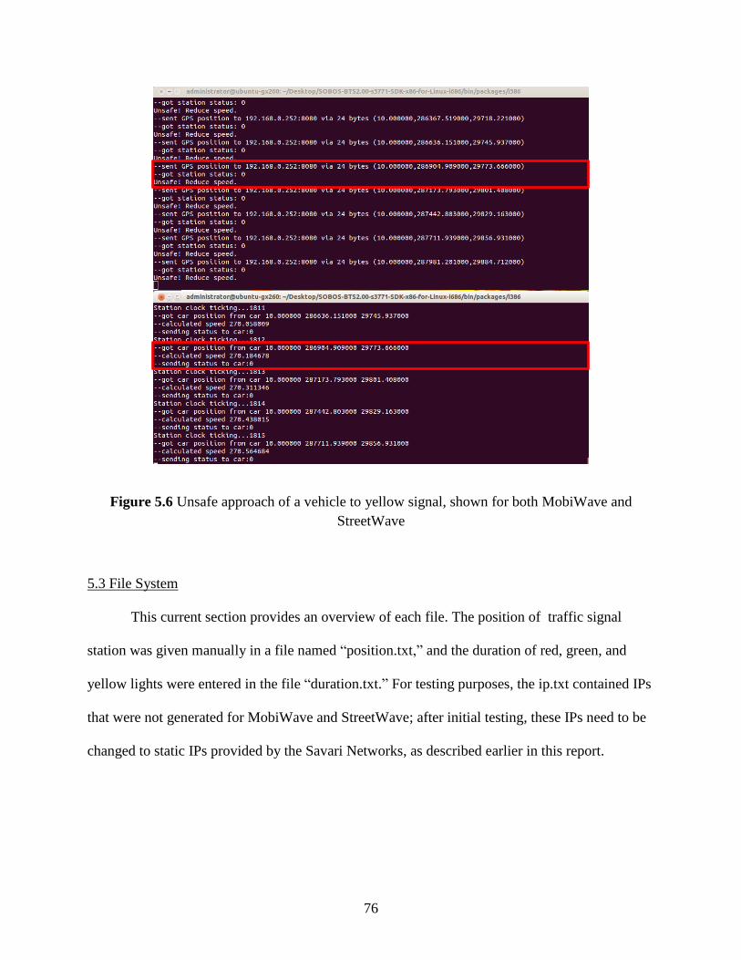
76
Figure 5.6 Unsafe approach of a vehicle to yellow signal, shown for both MobiWave and
StreetWave
5.3 File System
This current section provides an overview of each file. The position of traffic signal
station was given manually in a file named “position.txt,” and the duration of red, green, and
yellow lights were entered in the file “duration.txt.” For testing purposes, the ip.txt contained IPs
that were not generated for MobiWave and StreetWave; after initial testing, these IPs need to be
changed to static IPs provided by the Savari Networks, as described earlier in this report.
77
5.3.1General.c and General.h.
These header files include the information about the format that is being used by the GPS
device in the MobiWave. They also define type of IPs and GPS structure.
5.3.2 UDP.c and UDP.h
UDP stands for user data protocol. For any communication between two or more devices,
there should be a protocol to enable the safe and secure transmission of data, and also ensure that
the data is transferred in the same manner. All of these details fall under the category of user data
protocol, whether the connection between two devices is wired (such as development computer
to either MobiWave or StreetWave) or wireless (connection between MobiWave and
StreetWave). According to the specifications provided along with MobiWave and StreetWave,
these programs use static IPs, which enable developers to use proper socket programming. In any
package intended to work with these devices, the MobiWave IP is: 192.168.0.253, and the
StreetWave IP is: 192.168.0.252. In both cases, TCP port used was 8080 The username was root,
and the password was gems.
5.3.3 Car.c
The code to be housed in MobiWave is written in the file car.c. It translates the signal
received from StreetWave. This program is also responsible for obtaining GPS position from the
GPS device and putting it in the correct format to send over a wireless connection to StreetWave.
It should also be noted that whenever Mobiwave is communicating within itself, it should use IP:
127.0.0.1 and port 2947. This goes for any internal communication between MobiWave and the
inbuilt GPS.
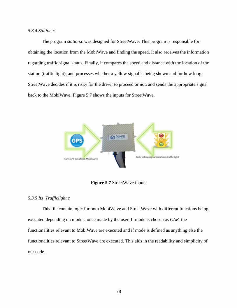
78
5.3.4 Station.c
The program station.c was designed for StreetWave. This program is responsible for
obtaining the location from the MobiWave and finding the speed. It also receives the information
regarding traffic signal status. Finally, it compares the speed and distance with the location of the
station (traffic light), and processes whether a yellow signal is being shown and for how long.
StreetWave decides if it is risky for the driver to proceed or not, and sends the appropriate signal
back to the MobiWave. Figure 5.7 shows the inputs for StreetWave.
Figure 5.7 StreetWave inputs
5.3.5 Its_Trafficlight.c
This file contain logic for both MobiWave and StreetWave with different functions being
executed depending on mode choice made by the user. If mode is chosen as CAR the
functionalities relevant to MobiWave are executed and if mode is defined as anything else the
functionalities relevant to StreetWave are executed. This aids in the readability and simplicity of
our code.
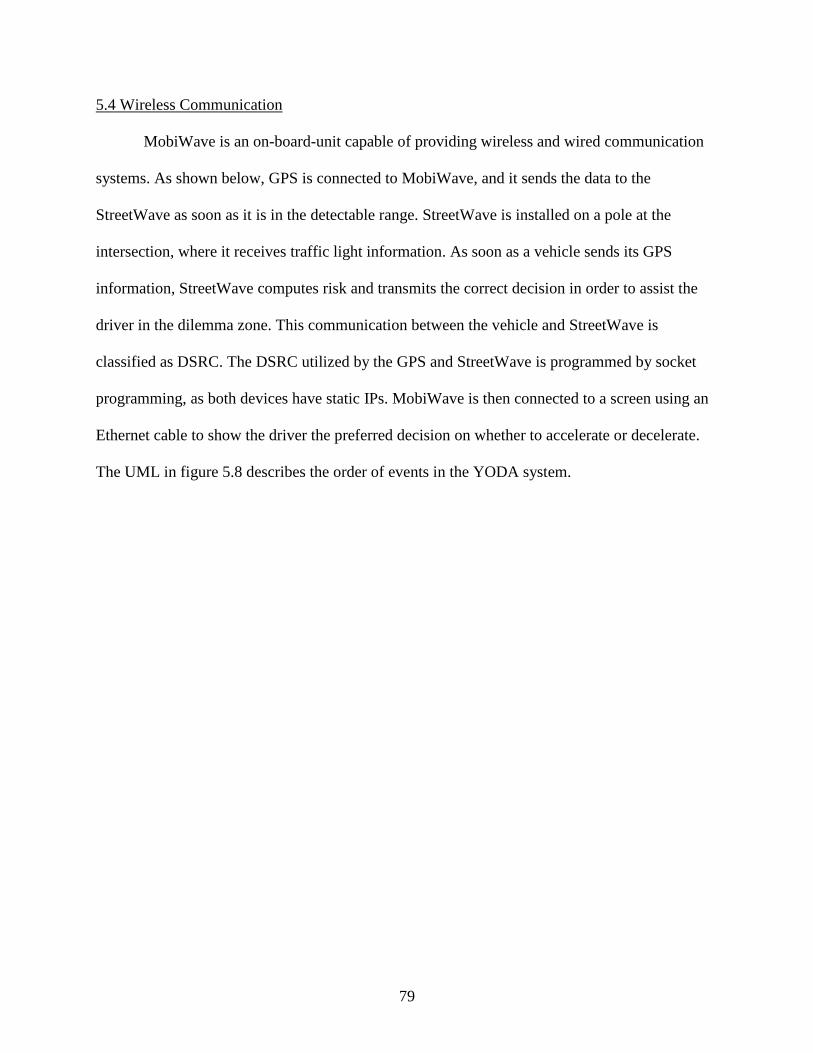
79
5.4 Wireless Communication
MobiWave is an on-board-unit capable of providing wireless and wired communication
systems. As shown below, GPS is connected to MobiWave, and it sends the data to the
StreetWave as soon as it is in the detectable range. StreetWave is installed on a pole at the
intersection, where it receives traffic light information. As soon as a vehicle sends its GPS
information, StreetWave computes risk and transmits the correct decision in order to assist the
driver in the dilemma zone. This communication between the vehicle and StreetWave is
classified as DSRC. The DSRC utilized by the GPS and StreetWave is programmed by socket
programming, as both devices have static IPs. MobiWave is then connected to a screen using an
Ethernet cable to show the driver the preferred decision on whether to accelerate or decelerate.
The UML in figure 5.8 describes the order of events in the YODA system.
80
Figure 5.8 Order of events in decision assistance
81
Chapter 6 Summary and Conclusions
This research examined the effect of information on drivers approaching high-speed
intersections. Data was collected at five intersections providing drivers with information via
AWF; an additional site lacking AWF was also evaluated. The probit model was used to model
driver decisions at the onset of yellow. The results were intended to inform conclusions on the
effects of AWF on the probability of stopping and illustrate their influence on perceived conflict
curves. Sites providing information through AWF curves displayed a tendency toward earlier
probability of stopping curves; in particular, Highway 2 and US-75 probability of stopping
curves differed drastically from the other studied sites. The shift at US-75 resulted in virtually all
drivers approaching the intersection with the potential for minor or severe conflict. The risk
associated with being downstream of the severe deceleration distance and upstream of the
maximum passing distance was calculated for a variety of speeds at each intersection. An overall
weighted average was then computed and compared to the crash histories. An association could
be seen in the comparison between the crash histories and the computed risks, as sites with large
severe deceleration risk had higher rear-end crash averages, and vice-versa. Therefore, it was
evident that providing drivers with information in advance of the intersection using AWF could
potentially increase the risk of rear-end accidents and RLR, as opposed to decreasing the risk for
drivers approaching these intersections. The information provided to the driver on stop and go
should be consistent with the actual duration of yellow. If the yellow time is longer and the
driver is incorrectly asked to stop, the result is confusion that results in riskier intersections. It
should also be noted that, when no information was provided, the critical time threshold for
stopping was very close to the actual yellow duration. This implies that drivers were inclined to
82
stop when the time to stop bar was greater than the yellow time, and were inclined to go when
the time to stop bar was less than yellow time.
The YODA system was developed, harnessing the insights gained regarding the impact
of information on driver decision making. The system consists of two units, MobiWave and
StreetWave. MobiWave is an on-board-unit capable of providing wireless and wired
communication systems. MobiWave sends the vehicle location information to StreetWave when
it is within a detectable range. Upon receiving this information, StreetWave computes the risks
for the vehicle, and sends back information on whether the vehicle can make it across the stop
bar within the remaining yellow time if the vehicle continues to travel at its current speed.
MobiWave displays this decision to the driver using a human machine interface.
6.1 Future Research
The future YODA system could incorporate the impacts of weather, time of day, volume
conditions, and the presence of other vehicles. Such site-specific information would make the
information provided to the driver more precise and case sensitive.
83
References
Akaike’s Information Criterion. Accessed June 12, 2009. http://www.modelselection.org/aic/.
Archer, J. 2004. “Methods for the assessment and prediction of traffic safety at urban
intersections and their application in micro-simulation modeling.” Royal Institute of
Technology, Department of Infrastructure, Stockholm, Sweden.
Armstrong, L. n.d. “Dedicated short range communications (DSRC) home.”
http://www.leearmstrong.com/Dsrc/DSRCHomeset.htm
Baker W. 1972. “An evaluation of the traffic conflict technique.” Highway Research Record,
384: 1-8.
Bonneson, J., and K. Zimmerman. 2005. "In-service evaluation of a detection-control system for
high-speed signalized intersections.” Report No. FHWA/TX-05/5-4022-01-1, Texas
Department of Transportation, Austin, TX.
Bonneson, J., K. Zimmerman, and M. Brewer. 2002. “Engineering countermeasures to reduce
red-light running,” Report No. 4027-2. Federal Highway Administration, Washington,
D.C.
Bonneson, J.A. and J. H. Son. 2003. “Prediction of expected red-light running frequency at urban
intersections.” Transportation Research Record, 1830: 38-47.
Chang, M., C. Messer, and A. Santiago. 1985. “Timing traffic signal change intervals based on
driver behavior.” Transportation Research Record, 1027: 20-30.
Cooper, P. 1973. “Predicting intersection accidents.” Ministry of Transport, Canada Road and
Motor Vehicle Traffic Safety Branch.
Cooper, D., and N. Ferguson. 1976. “Traffic studies at T-junctions: A conflict simulation
model.” Traffic Engineering and Control, 17, pg. 306-309.
Econometric Software, Inc. 2007. NLOGIT 4.0. Plainview, NY: author.
Elmitiny, N., X. Yan, C. Russo, and D. Nashar. 2010. “Classification analysis of driver’s stop/go
decision and red light running violation.” Accident Analysis and Prevention, 42, no. 1:
101-111.
Farraher, B. A., B. R. Wenholzer, and M. P. Kowski. 1999. “The effect of advance warning
flashers on red-light-running-A study using motion imaging recording system technology
at trunk highway 169 and Pioneer Trail in Bloomington, Minnesota.” Presented at the
69th
Annual Meeting of ITE, Las Vegas, Nevada.
84
Fazio, J., J. Holden, and N. Rouphail. 1993. “Use of freeway conflict rates as an alternative to
crash rates in weaving section safety analysis.” Transportation Research Record, 1401:
61-69.
Gates, T. J., D. A. Noyce, L. Laracuente, and G. Davis. 2006. “Effect of yellow-phase trigger on
driver’s behavior at high-speed signalized intersections.” Proceedings of 2006 IEEE
Conference on Intelligent Transportation Systems. Toronto, Canada, 683-688.
Gazis, D., R. Herman, and A. Maradudin. 1960. “The problem of amber signal light in traffic
flow.” Operations Research, 8, no. 1: 112-132.
Gettman, D. and L. Head. 2003. “Surrogate safety measures from traffic simulation models.”
Report No. FHWA-RD-03-050, Federal Highway Adninistration, U.S. Department of
Transportation, Washington D.C.
Gettman, D., L. Pu, T. Sayed, and S. Shelby. 2008. “Surrogate safety assessment model and
validation: Final report.” Publication No. FHWA-HRT-08-051. U.S. Department of
Transportation, Federal Highway Administration, Washington, D.C.
Gibby, A.R., S.P. Washington, and T.C. Ferrara. 1992. “Evaluation of high-speed isolated
signalized intersections in California.” Transportation Research Record, 1376: 45-56.
Glauz, W., K. Bauer, and D. Migletz. 1985. “Expected traffic conflict rates and their use in
predicting accidents.” Transportation Research Record, 1026: 1-12.
Glennon J., W. Glauz, M. Sharp, and B. Thorson. 1977. “Critique of the traffic-conflict
technique.” Transportation Research Record, 1026: 1-12.
Grayson, G. B. 1984. “The Malmo Study: A calibration of Traffic Conflict Techniques,” Report
R-84-12, Institute for Road Safety Research SWOV, Leidschendam, Netherlands.
Hakkert, A. S., and D. Mahalel. 1978. “The effect of traffic signals on road accidents with
special reference on the introduction of a blinking green phase.” Traffic Engineering &
Control, 19: 212-215.
Hauer, E., and P. Garder. 1986. “Research into the validity of the traffic conflict techniques.”
Accident Analysis & Prevention, 18: 471-481.
Hayward, J. 1972. “Near miss determination through use of a scale of danger.” Report no. TTSC
7715, Pennsylvania State University, PA.
Herman, R., P. L. Olson, and R.W. Rothery. 1963. “Problem of the amber signal light.” Traffic
Engineering and Control, 5: 298-304.
Hocherman, I., and J. Prashker. 1983. “Identification of high risk intersections in urban areas.”
Paper presented at the 1983 Annual Meeting of the PTRC, Brighton, U.K.
85
Hurwit, D. 2009. “Application of driver behavior and comprehension to dilemma zone definition
and evaluation.” Ph.D. diss., University of Massachusetts, Amherst, MA.
Hyden, C. 1987. “The development of a method for traffic safety evaluation: The Swedish traffic
conflicts technique.” Bulletin 70, University of Lund, Lund Institute of Technology,
Lund, Sweden.
ITE technical committee 18, (P. Parsonson, Chairman). 1974. “Small-area detection at
intersection approaches.” Traffic Engineering, February 1974, Institute of Transportation
Engineers, Washington D.C., 8-17.
Kim, W., J. Zhang, A. Fujiwara, T. Y. Jang, and N. Moon. 2008. “Analysis of stopping behavior
at urban signalized intersections.” Transportation Research Record, 2080: 84-91.
Knodler Jr., M. A., and D. Hurwitz. 2009. “An evaluation of dilemma zone protection practices
for signalized intersection control.” Report No. 2009-6, University of Massachusetts
Transportation Center, Amherst, MA, Vermont Agency of Transportation, Montpelier,
VT.
Koll, H., M. Bader, and K.W. Axhausen. 2004. “Driver behaviour during flashing green before
amber: A comparative study.” Accident Analysis & Prevention, 36: 273-280.
Kraay, J. H., & A. R. A. van der Horst. 1985. “Trautenfels-study: A diagnosis of road safety
using the Dutch Conflict observation technique DOCTOR.” Report R-85-53, Institute for
Road Safety Research SWOV, Leidschendam, Netherlands.
Kronborg, P., and F. Davidson. 1993. “MOVA and LHOVRA: Traffic signal control for isolated
intersections.” Traffic Engineering and Control, 34, no. 4: 193-200.
Kronborg, P., F. Davidsson, and J. Edholm. 1997. “Development and field trials of the SOS
algorithm for self optimising signal control at isolated intersections.” Publication TFK -
1997-05-07. Transportation Research Institute, Stockholm, Sweden.
Li, P. 2009. “Stochastic methods for dilemma zone protection at signalized intersections.”
Virginia Tech University, Blacksburg, VA.
Liu, Y., G. –L. Chang, R. Tao, T. Hicks, and E. Tabacek. 2006. “Empirical observations of
dynamic dilemma zones at signalized intersections.” Transportation Research Record,
2035: 122-133.
Liu, C., R. Herman, and D. Gazis. 1996. “Review of the yellow interval dilemma.”
Transportation Research Part A, 30: 333-348.
Mahalel, D. and J. N. Prashker. 1987. “A behavioral approach to risk estimation of rear-end
collisions at signlized intersections.” Transportation Research Record, 1114: 96-102.
86
Mahalel, D., and D. M. Zaidel. 1985. “Safety evaluation of a flashing-green light in a traffic
signal.” Traffic Engineering Control, 26: 79-81.
Mahalel, D., D. M. Zaidel, and T. Klein. 1985. “Driver’s decision process on termination of the
green light.” Accident Analysis & Prevention, 17: 373-380.
Mahmassani, S., and A. Probit. 1979. “Model of driver behavior at high speed isolated signalized
Intersections.” C.S. Working Paper No. 79-10, Massachusetts Institute of Technology.
Malkhamah, S., M. Tight, and F. Montgomery. 2005. “The development of an automatic method
of safety monitoring at Pelican crossings” Accident Analysis and Prevention, 37: 938-
946.
May A. D. 1968. “Clearance interval at flashing systems.” Highway Research Record, 221: 41-
71.
Messer, C. J., S. R. Sunkari, H. A. Charara, and R. T. Parker. 2003. “Development of advance
warning systems for end-of-green phase at high speed traffic signal.” Report 4260-4,
Federal Highway Administration, Washington, D.C., Texas Department of
Transportation, Texas Transportation Institute, Texas A & M University System.
Middleton, D., D. Jasek, H. Charara, and D. Mors. 1997. “Evaluation of innovative methods to
reduce stops to trucks at isolated signalized intersections.” Report No. TX-97/2972-S,
Texas Transportation Institute, Texas A&M University System.
Minderhoud, M. and P. Boy. 2001. “Extended time-to-collision measures for road traffic safety
assessment.” Accident Analysis & Prevention, 33: 89-97.
National Highway Traffic Safety Administration. 2007. Traffic Safety Facts 2006. Washington
D.C.: U.S. Department of Transportation, National Highway Traffic Safety
Administration.
Nebraska Department of Roads. 1999. Traffic crash facts 1998. Lincoln, NE: author.
Nebraska Department of Roads. 2000. Traffic crash facts 1999. Lincoln, NE: author.
Nebraska Department of Roads. 2001. Traffic crash facts 2001. Lincoln, NE: author.
Nebraska Department of Roads. 2002. Traffic crash facts 2002. Lincoln, NE: author.
Nebraska Department of Roads. 2003. Traffic crash facts 2003. Lincoln, NE: author.
Nebraska Department of Roads. 2004. Traffic crash facts 2004. Lincoln, NE: author.
Nebraska Department of Roads. 2005. Traffic crash facts 2005. Lincoln, NE: author.
87
Nebraska Department of Roads. 2006. Traffic crash facts 2006. Lincoln, NE: author.
Nebraska Department of Roads. 2007. Traffic crash facts 2007. Lincoln, NE: author.
Nebraska Department of Roads. 2008. Traffic crash facts 2008. Lincoln, NE: author.
Nebraska Department of Roads. 2009. Traffic crash facts 2009. Lincoln, NE: author.
Newton, C., R. Mussa, E. Sadalla, E. Burns, and J. Matthias. 1997. “Evaluation of an alternative
traffic light change anticipation system.” Accident Analysis and Prevention, 29, no. 2:
201-209.
Olson, P., and R. Rothery. 1962. “Driver response to amber phase of traffic signals.” Highway
Research Board, 330: 40-51.
Paddock, R. 1974. “The traffic conflict technique: An accident prediction method.” Ohio
Department of Transportation, Division of Highways, Bureau of Traffic Control.
Pant, P. D., and X. H. Huang. 1992. “Active advance warning signs at high-speed signalized
intersections: Results of a study in Ohio.” Transportation Research Record, 1368: 18-26.
Pant, P. D., and Y. Xie. 1995. “Comparative study of advance warning signs at high-speed
signalized intersections.” Transportation Research Record, 1495: 28-35.
Papaioannou, P. 2007. “Driver behavior, dilemma zone and safety effects at urban signalised
intersections in Greece.” Accident Analysis and Prevention, 30, no. 1: 147-158.
Parsonson, P. 1978. “Signalization of high speed, isolated intersections.” Transportation
Research Record, 681: 34-42.
Parsonson, P. S., and A. Santiago. 1980. “Design standards for timing-The traffic signal
clearance period must be improved to avoid liability.” Compendium of Technical Papers,
1980 ITE Conference, 67-71.
Perkins, S. R., and J. I. Harris. 1968. “Traffic conflict characteristics: Accident potential at
intersections.” Highway Research Record, 225: 45-143.
Rakha, H., I. El-Shawarby, and J. R. Setti. 2007. “Characterizing driver’s behavior on signalized
intersection approaches at the onset of a yellow-phase trigger.” IEEE Transactions on
Intelligent Transportation System, 8, no. 4: 630-640.
Research and Innovative Technology Administration (RITA) • U.S. Department of
Transportation (US DOT), http://www.rita.dot.gov/
Savari. n.d. www.Savarinetworks.com.
88
Sayed, T, V. Homoyaoun, and F. Rodriquez. 1999. “Advance warning flashers, do they improve
safety?” Transportation Research Record, 1692: 30-38.
Sharma, A. 2008. “Integrated behavioral and economic framework for improving dilemma zone
protection systems.” Ph.D. diss., Purdue University.
Sharma, A., D. Bullock and S. Peeta. 2011. “Estimating dilemma zone hazard function at high
speed isolated intersection.” Transportation Research Part C: Emerging Technologies,
19, no. 3: 400-412.
Sharma, A., D. Bullock, and S. Peeta. 2007. “Recasting dilemma zone design as a marginal
costs-benefits problem.” Transportation Research Record, 2035: 88-96.
Sharma, A., M. Harding, B. Giles, D. Bullock, J. Sturdevant, and S. Peeta. 2008. “Performance
requirement and evaluation procedures for advance wide area detector.” Paper presented
at the 87th Annual Meeting of the Transportation Research Board, Washington, D.C.
Sheffi, Y., and M. Mahmassani. 1981. “A model of driver behavior at high speed signalized
intersections.” Transportation Science, 15, no. 1: 51-61.
Sivak, M., P. L. Olson, and K. M. Farmer. 1982. “Radar measured reaction times of unalerted
drivers to brake signals.” Perceptual and Motor Skills, 55: 594.
Spicer, B. A. 1972. “A traffic conflict study at an intersection on the Andoversford by-pass.”
TRRL Report LR 520, Transport and Road Research Laboratory, Road User
Characteristics Division, Safety Department.
Stander, H. J. 1989. “Timing of the change interval at traffic signals.” Presented at the Annual
Transportation Convention, Pretoria, South Africa.
Van der Horst, A. R. A. 1984. “The ICTCT calibration study at Malmo: a quantitative analysis of
video-recordings.” Report IZF 1984-37, TNO Institute for Perception, Soesterberg,
Netherlands.
Van der Horst, A. R. A. 1990. “A time-based analysis or road user behaviour in normal and
critical encounters.” Ph.D. diss., Delft University of Technology, Delft, Netherlands.
Van der Horst, R. and A. Wilmink, 1986, “Driver’s Decision-Making at Signalized Intersections:
An Optimization of the Yellow Timing,” Traffic Engineering & Control. pp. 615-622.
Wavetronix. 2009. “SmartSensor Advance.”
www.wavetronix.com/en/products/smartsensor/advance/safearrival. Accessed February
9, 2011.
89
Wei, H., Z. Li, and Q. Ai. 2009. “Observation-based study of intersection dilemma zone
natures.” Journal of Transportation Safety & Security, 1, no. 4: 282-295.
Williams, W. L. 1977. “Driver behavior during yellow interval.” Transportation Research
Record, 644: 75-78.
Wortman, R. H., and J. S. Matthias. 1983. “Evaluation of driver behavior at signalized
intersections.” Transportation Research Record, 904: 10-20.
Xsens Technologies B.V. 2009. MTi-G Quick setup: Getting started with your MTi-G (p. 4).
Enschede, Netherlands: author.
Zeeger, C., 1977. “Effectiveness of green-extension systems at high-speed intersection.”
Research Report 472, Bureau of Highways, Kentucky Department of Transportation,
Lexington, Kentucky.
Zimmerman, K. 2007. “Development of a second generation detection-control system for safer
operation of high-speed signalized intersections.” Report No. TRB-NCHRP-115, Texas
Transportation Institute, Texas A&M University System.
Related Documents