Replacing Income Taxation with Consumption … in income taxation in Japan along with increases in consumption taxation to stabilize the debt to output ratio. In particular, we consider

CIGS Working Paper Series No. 17-008E

General Incorporated Foundation

The Canon Institute for Global Studies 一般財団法人 キヤノングローバル戦略研究所

Phone: +81-3-6213-0550 http://www.canon-igs.org

※Opinions expressed or implied in the CIGS Working Paper Series are solely those of the

author, and do not necessarily represent the views of the CIGS or its sponsor.

※CIGS Working Paper Series is circulated in order to stimulate lively discussion and

comments.

※Copyright belongs to the author(s) of each paper unless stated otherwise.

Replacing Income Taxation with

Consumption Taxation

in Japan

Gary D. Hansen

Department of Economics, UCLA

Selahattin Imrohoroglu

Marshall School of Business, University of Southern California

International Senior Fellow, The Canon Institute for Global Studies

October, 2017

Replacing Income Taxation with Consumption Taxation

in Japan∗

Gary D. Hansen†and Selahattin Imrohoroglu‡

October 4, 2017

Abstract

Over the past two decades, Japan has suffered from low economic growth and a largeand growing debt to output ratio. Furthermore, Japan anticipates significant increasesin future government expenditures due to an aging population. These problems haveled Japan to introduce a consumption tax rate in an attempt to raise revenues, and,more recently, to reduce the statutory corporate income tax rate to raise investmentand output growth. In this paper we study the growth and welfare consequences of areduction in income taxation in Japan along with increases in consumption taxationto stabilize the debt to output ratio. In particular, we consider various unanticipatedtax reforms using the model described in Hansen and Imrohoroglu (2016). We findthat while output per working age population is projected to be roughly constantbetween 2015 and 2021 in the benchmark equilibrium representing the status quo,under alternative policies considered, output could be as much as 15% higher by 2021.

∗ We would like to thank Nao Sudo for comments and suggestions at all stages of this research. The authors also thank theparticipants of the seminars and conferences at Kyoto University, Universitat Autonoma de Barcelona, Universitat Carlos IIIde Madrid, University College London, and the Annual Meetings of the Society for Economic Dynamics, Edinburgh.

†Department of Economics, UCLA, [email protected].‡Marshall School of Business, University of Southern California, [email protected].

1 Introduction

In the last ten to twenty years, policy makers in Japan have continuously grappled withtwo major policy issues: recovering from low rates of economic growth and achieving fiscalconsolidation. Japan’s economy has experienced dismal performance since the early 1990s.The rate of growth of real Gross Domestic Product (GDP) was 4.4% between 1972 and 1990,but has dropped to only 1.0% between 1991 and 2015. In an influential paper, Hayashi andPrescott (2002) coined the term “the Lost Decade” for the prolonged stagnation during the1990s. The stagnation has continued until the current years making it the “Lost Decades.”1

Partly because large scale fiscal stimulus packages were conducted during the lost decade,Japan’s economy has accumulated the highest net debt to output ratio among developedeconomies. Going forward, the debt to output ratio is expected to further rise due to theprojected increase in government expenditures related to the aging of the Japanese society.

Other things being equal, a higher dependency ratio leads to higher expenditures onpublic health expenditures and pensions, which in turn adds to the fiscal imbalance. Figure1 displays the predicted time paths of the government purchases and transfer paymentsrelative to GNP.2 Both series exhibit a clear positive trend over the next couple of decades.

This paper studies unanticipated changes in tax policy that involve lowering incometax rates (labor income tax rates as well as capital income tax rates) shifting away from in-come taxation toward consumption taxation. The goal is to study the growth consequencesas well as the welfare consequences of such policy reforms. We carry out this analysis usingthe model developed in Hansen and Imrohoroglu (2016). In that paper, the implicationsof policies aimed at reducing Japan’s debt to output ratio are studied in an environmentwithout uncertainty–one where economic agents have perfect foresight about future govern-ment policy. Here, a similar policy is used to stabilize debt in the long run, but, in addition,unanticipated changes in tax rates are assumed to be introduced at a specified date. Whatwe find is that policies that generate a lot of additional growth in the short run do notnecessarily lead to the highest welfare relative to a benchmark case, which is based on thepolicy studied in Hansen and Imrohoroglu (2016). In particular, we find that policies thatreduce income taxation but postpone increasing consumption taxes until Japan’s debt tooutput ratio reaches some threshold provides lower growth and higher welfare relative to apolicy that raises consumption taxes simultaneously with the reduction in income taxes inorder to replace lost revenue.

1As pointed out in Hayashi and Prescott (2002), a slowdown of GDP growth during the 1990s and beyondhas come together with a TFP slowdown. Though our paper treats TFP movements as exogenous, given thatwe focus on implications of changes in tax policy, a good number of economists have explored reasons behindthe TFP slowdown. Caballero, Hoshi, and Kashyap (2008) argue that zombie-lending has created stagnationby enabling capital and labor to remain in firms that should instead go bankrupt, leading to lower aggregateproductivity than would otherwise be the case. Kwon, Narita, and Narita (2015) use plant level data andfind that resource misallocation, labor in particular, contributed negatively to aggregate productivity growth.Guner, Ventura, and Yi (2008) develop a model that delivers an efficient size distribution of firms, and arguethat departures from the efficient size distribution lead to lower productivity. Buera, Moll, and Shin (2013)develop a theory in which well-intended policies may have a sizable negative long-run effect on aggregateoutput and productivity.

2These time paths incorporate projections of future government purchases and transfer payments made byFukawa and Sato (2009) that use detailed information from the Employees Pension Insurance, the NationalPension, and the government-managed Health Insurance and Long-term Care Insurance.

1

1980 1990 2000 2010 2020 2030 2040 2050 2060 2070 20800.05

0.1

0.15

0.2

0.25

G/Y

1980 1990 2000 2010 2020 2030 2040 2050 2060 2070 20800.05

0.1

0.15

0.2

0.25

TR

/Y

Figure 1: Government Expenditures to GNP: Data 1981-2014, projections 2015-2050

Our motivation is drawn from economic policies that have recently been introducedin Japan to achieve the two policy goals–higher growth and lower debt to output. TheJapanese government has launched two economic policy packages independently, each ofwhich involves tax reform. One involves reductions in the corporate tax rate and the otherbrings about increases in the consumption tax rate. The corporate tax reductions are a partof the policy package known as the “three arrows” proposed by Prime Minister Shinzo Abein 2013.3 In fiscal year (FY) 2014, the effective corporate income tax rate was 34.62%. It hassince been reduced to 32.11% with plans for further reductions to 29.97% in FY 2016/2017and 29.74% in FY 2018. The eventual goal is a tax rate of 25%.

The consumption tax in Japan was equal to 5% from 1997 to 2013. Given projectedincreases in social security benefits, however, the government announced a “ComprehensiveReform of Social Security and Tax” in 2013, stating that consumption tax rates would beraised eventually to 10% and the revenues would be secured as financial resources to fundsocial security. The consumption tax rate was raised from 5% to 8% in 2014 as planned, buta further increase from 8% to 10% that was scheduled for 2015 was postponed and is nowscheduled for 2019. These tax reforms are being implemented independently. On the whole,however, they will change the Japanese tax structure so that it relies more on consumptiontaxation and less on income taxation.

The model economy we use is a neoclassical growth model built upon Hayashi andPrescott (2002), Chen, Imrohoroglu, and Imrohoroglu (2006), and Hansen and Imrohoroglu(2016). Our model incorporates into an otherwise standard neoclassical growth model twofeatures. The first is that government bond holdings are assumed to provide utility to

3The “three arrows” consist of monetary easing, fiscal stimulus, and policies designed to increase economicgrowth. Reductions in the corporate income tax rates belong to the third arrow.

2

Japanese households. The motivation for this is to account for large domestic holding ofJapanese Government Bonds at very low interest rates.4 The second is a debt stabilizationpolicy rule followed by the government. As in Hansen and Imrohoroglu (2016), once the debtto output ratio reaches a critical level, the Japanese government automatically increases theconsumption tax rate to stabilize the debt.5

In contrast to the experiments conducted in Hansen and Imrohoroglu (2016) in whicheconomic agents have perfect foresight, simulations here are conducted in two steps to reflectthe unanticipated nature of the tax reforms studied. First, we compute the equilibriumfuture time path of endogenous variables including output, tax revenue, and welfare underthe hypothetical scenario that no tax reforms are implemented. That is, the tax structureis unchanged from 2014 and beyond. Our simulations take as exogenous inputs forecastsof future government purchases and transfer payments made by Fukawa and Sato (2009)and projections of future population growth rates produced by the Japanese government.6

Taking state variables for 2015 as given from the first step, the second step computes theequilibrium path from 2015 on under the assumption that an unanticipated tax reform isintroduced in 2015.

The model-generated equilibrium path indicates that under no tax reform, Japan’seconomy will continue experiencing stagnant GDP growth and rapid government debt accu-mulation that quickly exceeds the critical level. When an unexpected elimination of corporatetaxes is introduced in 2015 along with an increase in consumption taxes to replace the lostrevenue, government debt still reaches the critical level at the same date, but the averageannual growth rate of output per person over the following six years is one percent higherthan if no reform is introduced. While reducing corporate tax rates is consistent with actualtax reforms proposed in Japan, we also study effects of replacing labor income taxation withconsumption taxation for comparison purposes and find that further growth and welfareimprovements can be achieved.

Reducing the capital income tax rate, however, jeopardizes fiscal consolidation byreducing tax revenue. In particular, we find that a 3.75 percentage point increase in the theconsumption tax rate is needed to replace the lost revenue if the capital income tax rate isreduced to 20%. However, in the long run steady state, the consumption tax is only about 80basis points higher than it is in our benchmark where there are no reductions in the capitalincome tax rate other than those Japan has already implemented (a capital income tax rateof 34%). If the capital income tax rate is reduced to zero, the steady state consumption taxrate is 2.78 percentage point higher than in the benchmark. On the other hand, reductionsin the labor income tax rate would require a much larger increase in the consumption tax to

4Sakuragawa and Hosono (2010) employ an alternative approach that incorporates intermediation coststo obtain low equilibrium interest rates on government debt.

5In our theoretical model, there is no upper bound to the feasible debt to output ratio. However, weimpose an upper bound under the assumption that for reasons not modeled, there is a practical upper boundto this ratio.

6Following Hansen and Imrohoroglu (2016), our simulation incorporates projections made by the NationalInstitute of Population and Social Security Research for the population growth rate, and projections madeby Fukawa and Sato (2009) for health insurance and social security benefits that constitute important partsof the government purchases and transfer payments. Admittedly, Japan might choose to renege on thepromises to retirees that underlie the forecasts of Fukawa and Sato (2009). However, our analysis will bedone under the assumption that these promises will be kept.

3

replace lost revenue. A decrease from a labor income tax rate of 33% in our benchmark to20% would require a 13.17 percentage point increase in consumption taxes to replace the lostrevenue. In the long run steady state, the consumption tax rate would still be 12 percentagepoints higher than in the benchmark.

Our paper is closely related to the two strands of the literature on tax structure.Both of them have attracted attention from a large number of macroeconomists over along period of time. One strand, including Barro (1990), Easterly and Rebelo (1993), andMendoza, Milesi-Ferretti, and Asea (1997), examines growth implications of tax structure.7

For instance, Barro (1990) theoretically shows that under some conditions income taxationmay hamper economic growth. Along the line of his theoretical prediction, recent studiesby Knellera, Bleaney, and Gemmell (1999) and Arnold (2008) document using the data ofOECD countries that income taxation or property taxation reduces growth while consump-tion taxation does not. The other strand of literature, including Trabandt and Uhlig (2011),Nutahara (2015), and Hansen and Imrohoroglu (2016), explores how tax structure mattersfor fiscal sustainability. Among them, our paper is closest to Hansen and Imrohoroglu (2016)that studies how much either consumption taxation or labor income taxation must increaseto stabilize the growing government debt in Japan.

The structure of this paper is as follows. Section 2 describes the details of our model.Section 3 describes the calibration of the model and the simulation methodology. The resultsobtained from simulating various tax reforms are presented in Section 4. Section 5 concludes.

2 Model

In this section we describe the details of our model, which is similar to the model of Hansenand Imrohoroglu (2016). The notation employed uses upper case letters to denote variablesthat are per capita values that grow along a balanced growth path. Lower case letters denotevariables that are stationary along a balanced growth path. The time period of the modelis one year.

The economy is populated by a representative household with Nt members at timet. The size of the household is assumed to grow at a time-varying growth factor ηt so thatNt+1 = ηtNt.

The fiscal analysis in this paper takes as given time series on tax rates, governmentspending (Gt), transfer payments (TRt), the working age population (Nt), and total factorproductivity (At), where actual time series are used from 1981-2014. Forecasts and assump-tions are used to extend these series to 2060 and beyond. In addition, we assume that the taxrates, the ratios of government purchases and transfer payments to output, and the growthrates of Nt and At are all eventually constant and the economy converges to a balancedgrowth path. Hours worked (ht), consumption (Ct), output (Yt), the stock of capital (Kt),tax revenues, government debt (Bt), and the price of government bonds (qt), from 1981 intothe infinite future are endogenously determined by the model.

7There are also a number of theoretical papers including Judd (1985), Chamley (1986) that study therelationship between the level of output and tax rates.

4

2.1 Government

The government is assumed to collect revenue from taxing household consumption at the rateτc,t, labor income at the rate τh,t, capital income at the rate τk,t, and interest on governmentbonds at the rate τb,t. Given time series for Gt and TRt, the quantity of one-period discountbonds (Bt+1) that are issued by the government is determined by the following budgetconstraint (where all quantities are in per capita terms):

Gt + TRt +Bt = ηtqtBt+1 + τc,tCt + τh,tWtht (1)

+τk,t(rt − δ)Kt + τb,t(1− qt−1)Bt.

Here, in addition to variables already defined, Wt and rt denote the wage rate andthe return to capital, and δ is the depreciation rate of capital.

The government is also assumed to be subject to a “debt sustainability” rule thatforces the government to retire debt when the debt to output ratio reaches some arbitraryvalue bmax that we specify. We denote the date at which this limit is reached by T1. Weinclude this feature for two reasons. First, the solution procedure we use for computingequilibrium paths requires that the economy ultimately converge to a steady state with aconstant bond to output ratio. Without some additional constraint, this convergence wouldnot be guaranteed. Second, while there is no natural limit to how much debt the governmentin our model can issue, such a limit almost certainly exists in actual economies.

Along a given transition path, taxes and transfers are initially determined accordingto calibrated values. These values may differ across the experiments that we conduct. Oncethe debt to output ratio hits the threshold level, bmax at T1, two fiscal instruments–the level oftransfers and the consumption tax rate–become endogenous in order to insure convergenceto the terminal steady state that we specify. Denote the initial calibrated values for theconsumption tax and transfers for each date t by τCc,t and TR

Ct . In addition, denote the value

of the consumption tax rate and the debt to output ratio in our steady state by τ c and b.Given this, the actual values for τc,t and TRt are determined as follows:

τc,t =

τCc,t if t < T1 (i.e. Bs/Ys ≤ bmax for all s ≤ t)

τ c + π if T1 ≤ t < T2 (i.e. Bs/Ys > bmax for some s ≤ t and Bt/Yt > b)

τ c if t ≥ T2 (i.e. Bt/Yt ≤ b),

(2)

TRt =

TRCt if t < T1

TRCt − 0.08Yt if T1 ≤ t < T2

TRCt − 0.08Yt − κ(Bt − bYt) if t ≥ T2 ,

(3)

According to equation (2), once the upper bound on debt is reached, the consumptiontax is set equal to its steady state value, τ c, plus some constant π, where π is the smallestbasis point increase in this tax rate such that the debt to output ratio will begin to declineafter date T1. Once the debt to output ratio becomes less than or equal to b, the consumptiontax rate is set equal to its steady state value. We denote this date by T2.

5

In addition, as shown in equation (3), at date T1 transfers are reduced by 8% of outputreflecting our assumption that “tax base broadening”will be implemented at the time debt-reducing reform is required.8 At date T2 transfers are adjusted to retire (or augment) thestock of government debt [determined by equation (1)] so that the debt to output ratioconverges to the desired steady state value, b. Here, κ is a positive fraction that determineshow quickly the bond to output ratio converges to its steady state value. We use a value ofκ = 0.1 in our quantitative exercises.

2.2 Household’s Problem

The household at time 0 is endowed with initial holdings of per capita physical capitalK0 > 0, and real, one-period, zero-coupon, discount bonds B0. In addition, each memberof the household is endowed with one unit of time each period that can be used for mar-ket activities ht or leisure 1 − ht. Given a sequence of wages, rental rates for capital andgovernment bond prices {Wt, rt, qt}

∞

t=0, as well as a sequence of tax rates on consumptionexpenditures, tax rates on income from labor, capital and holdings of government bonds, andper-capita transfer payments {τc,t, τh,t, τk,t, τb,t, TRt}

∞

t=0, the household chooses a sequence ofper member consumption, hours worked, capital, and bond holdings {Ct, ht, Kt+1, Bt+1}

∞

t=0

to solve the following problem:

max∞∑

t=0

βtNt[logCt − αh1+1/ψt

1 + 1/ψ+ φ log(µt+1 +Bt+1)] (4)

subject to

(1 + τc,t)Ct + ηtKt+1 + qtηtBt+1 = (1− τh,t)Wtht + [(1 + (1− τk,t)(rt − δ)]Kt (5)

+[1− (1− qt−1)τb,t]Bt + TRt,

where K0 > 0 and B0 are given initial conditions. The parameter β denotes the household’ssubjective discount factor. The disutility of work is described by −α < 0 and φ > 0 denotesthe household’s preferences for government bonds. We use ψ to denote the intertemporalelasticity of substitution (IES) of labor.

The household’s maximization is subject to a budget constraint [equation (5)] whereafter-tax consumption expenditures and resources allocated to accumulation of capital andbond holdings are financed by after-tax labor income, after-tax capital income and holdingsof capital, after-tax proceeds of bond holdings chosen in the previous period, and transferpayments from the government. Here Kt+1 and Bt+1 are per capita holdings of capital andbonds at time t + 1. ηtKt+1 and ηtBt+1 expresses the same quantities per capita at time t.

8As in Hansen and Imrohoroglu (2016) we have abstracted from deductions, exclusions, and progressivetax rates that characterize the Japanese tax code. By setting income tax rates equal to the average marginaltax rate in Japan, the amount of revenue raised in our model exceeds that actually raised by the Japanesetax system by 8% of output. In our basic calibration, we assume this excess revenue is added to transferpayments as a lump sum tax rebate to households. Tax broadening in our context means that we eliminatethis tax rebate and allow this revenue to be used to lower the level of debt each period.

6

Since about 95% of the Japanese government bonds are held domestically, we assumethat Japan is a closed economy where all debt is held by Japanese citizens, i.e. the membersof the household in our model. In addition, Japanese government bonds historically havehad yields less than the return to physical capital. As a result, we introduce governmentdebt in the utility function, with φ > 0.9 10

Finally, µt+1 is a parameter that limits the curvature of the period utility functionover bonds. Essentially, it represents assets that might be perfect substitutes to Japanesegovernment issued bonds in generating utility to households.11 We allow this parameter tomove at the same rate of balanced growth as the rest of the economy so that the detrendedversion is a constant. In particular, µt = µA

1/(1−θ)t .

2.3 Firm’s Problem

A stand-in firm operates a constant returns to scale Cobb-Douglas production technology

NtYt = At(NtKt)θ(Ntht)

1−θ

Nt+1Kt+1 = (1− δ)NtKt +NtXt.

Capital depreciates at the rate δ. The income share of capital is given by θ. At is total factorproductivity which grows exogenously at the rate γt, so we have At+1 = γtAt. Per capitagross investment is denoted by Xt.

The firm is assumed to hire labor and rent capital from households each period tomaximize profits, taking the wage rate Wt and rental rate rt as given.

2.4 Equilibrium

Given a government fiscal policy {Gt, TRt, Bt, τh,t, τk,t, τc,t, τb,t}∞

t=0, a debt sustainability rule{κ, b, bmax}, and the paths of working age population {Nt}

∞

t=0 and technology {At}∞

t=0, a com-petitive equilibrium consists of an allocation {Ct, ht, Kt+1, Bt+1}

∞

t=0, factor prices {Wt, rt}∞

t=0

and the bond price {qt}∞

t=0 such that

• the allocation solves the household’s problem [equations (4) and (5)],

• the government budget constraint and debt sustainability rule, given by equations (1)- (3), is satisfied each period,

9For example, consider a simplified version of the model in which the representative household solvesmax

∑∞

t=0βt {log ct + φ log bt+1} subject to ct + kt+1 + qtbt+1 = wt + rtkt + bt + (1 − δ)kt. The first order

conditions are given by 1

ct= β Rt

ct+1, φbt+1

− qtct+ β

ct+1= 0, andRt = rt+1−δ. Steady-state implies q− 1

R= φc

b> 0,

which means that the return on k, denoted by R, dominates that on b which is equal to 1/q.10While our assumption of bonds providing utility in a neoclassical growth model implies that capital

earns a higher return than government debt, it also implies that the optimal quantity of debt is unlimited.Nakajima and Takahashi (2017) studies the optimal debt to output ratio for Japan using a micro-foundedmodel similar to Aiyagari and McGrattan (1998) in which there are both costs and benefits associated withgovernment debt.

11This parameter helps us to match the volatility of bond prices.

7

• the market for bonds clears,

• firms maximize profits and the labor market and capital rental markets clear, whichimplies that Wt = (1− θ)AtK

θt ht

−θ and rt = θAtKθ−1t ht

1−θ.

• and the goods market clears: Ct + [ηtKt+1 − (1− δ)Kt] +Gt = Yt,

2.5 Detrended Equilibrium Conditions

In this subsection we derive the detrended equilibrium conditions to use in solving the modelnumerically. Given a trending per capita variable Zt we obtain its detrended per capitacounterpart by

zt =Zt

A1/(1−θ)t

.

The first set of detrended equilibrium conditions is given below.

(1 + τc,t+1)γ1/(1−θ)t ct+1

(1 + τc,t)ct= β[1 + (1− τk,t+1)(rt+1 − δ)], (6)

φ

µ+ bt+1

+βηt[1− (1− qt)τb,t+1]

(1 + τc,t+1)ct+1

=qtηtγ

1/(1−θ)t

(1 + τc,t)ct, (7)

αh1/ψt =

(1− τh,t)wt(1 + τc,t)ct

, (8)

yt = kθth1−θt , (9)

ηtγ1/(1−θ)t kt+1 = (1− δ)kt + xt. (10)

Equation (6) is the typical Euler equation arising from the choice of capital stock attime t. The bond Euler equation is given by (7). The first order condition for hours workedis shown in equation (8). The production function and the law of motion for capital aregiven in equations (9) and (10), respectively. The budget constraint for the household isgiven below in equation (11)

(1 + τc,t)ct + ηtγ1/(1−θ)t kt+1 + qtηtγ

1/(1−θ)t bt+1 (11)

= (1− τh,t)wtht + [1− (1− qt−1)τb,t]bt + trt + [1 + (1− τk,t)(rt − δ)]kt.

The government budget equation is given by equation (12)

gt + trt + bt = qtηtγ1/(1−θ)t bt+1 + τc,tct + τh,twtht (12)

+τk,t(rt − δ)kt + τb,t(1− qt−1)bt.

Finally, the market clearing conditions are given below in equations (13), (14) and(15)

rt = θkθ−1t h1−θt , (13)

wt = (1− θ)kθt h−θt , (14)

ct + xt + gt = yt. (15)

Hence we have 9 equations, (6) through (14), in 9 unknowns{ct, xt, ht, yt, kt+1, bt+1, qt, wt, rt} at each time period t.

8

2.6 Steady-State Solution

In this subsection we describe how we compute the steady state equilibrium and how itdepends on the experiments we consider in section 4.

For a variable zt, we will denote its steady state value with z. Also, let z denote z/y,the ratio of z to the steady state value of output.

Imposing steady state, equations (6) and (10) become k = βθ(1−τk)

γ1/(1−θ)−β[1−(1−τk)δ]

and

x = ηγ1/(1−θ) + δ − 1.Using projections from Fukawa and Sato (2009), we obtain detrended values for gt and

trt and assume that these are constant after 2050. In particular, g = g2050 and tr = tr2050.

Given a value for τc, values for h, c and y are given by h =[(1−θ)(1−τh)α(1+τc)c

]ψ/(1+ψ),

c = 1− x− g, and y = kθ/(1−θ)h, where g = g/y.Using the steady state version of equation (7), we obtain

q =φ(1 + τc)c+ βη(1− τb)b+ µ

η [γ1/(1−θ) − βτb] (µ+ b), where b = by.

This plus the steady state version of the government budget constraint (12) can beused to obtain values for q and τc. The steady state government budget constraint can bewritten

g + tr +[1− qηγ1/(1−θ)

]b = τ cc+ (1− θ)τh + τk(θ − δk) + τb(1− q)b.

We will assume that the values of g, tr, τb and b are the same across all steady states.However, the income tax rates τh and τk are different across experiments. As a result, allother aspects of the steady state, including the consumption tax rate τc and steady statebond holdings b, will differ across experiments.

2.7 Solution Procedure

We take as given a value for k1981 and a sequence {τh,t, τb,t, τk,t, ηt, γt, gt}∞

t=1981, where theelements of this sequence are constant beyond some date. These constant values along withτc, g = g2050 and tr = tr2050 determine the steady state to which the economy ultimatelyconverges. We use a shooting algorithm, similar to that in Hayashi and Prescott (2002),Chen, Imrohoroglu, and Imrohoroglu (2006) and Hansen and Imrohoroglu (2016), to deter-mine the value of c1981 (or, equivalently, k1982) such that the sequence of endogenous variables{ct, xt, ht, yt, kt+1, bt+1, qt, wt, rt} determined by equations (6) through (14) converges to thesteady state. That is, the shooting algorithm guarantees that the capital stock sequencesatisfies the transversality condition. In addition, the fiscal sustainability rule determinesthe sequence of transfers and consumption taxes, {trt, τc,t}, that guarantees that the bond

to output ratio is equal to b in the steady state achieved in the limit.While the above procedure is used to compute our benchmark transition, the pri-

mary topic of this paper is to consider the consequences of unanticipated policy changes in2015. To do this, we first compute the transition path to the steady state for our bench-mark calibration. Then, taking c2014 (or, equivalently, k2015) as given, we compute a new

9

transition from 2015 to the steady state associated with policy under consideration that wasunanticipated prior to 2015. The full transition from 1981 is formed by splicing togetherthe benchmark transition through 2014 with the alternative policy transition beginning with2015.

3 Calibration

The structural parameters of our model are calibrated based on information from the sampleperiod, which consists of annual data from 1981 to 2014. We take the capital-output andbond-output ratios in 1981 as initial conditions and use the sample paths for total factorproductivity (TFP), population growth rates, tax rates, government purchases and transferpayments as exogenous inputs to the model. In addition we make assumptions about the val-ues for these exogenous variables beyond the sample period in order to calculate equilibriumtransition paths from 1981 toward the eventual steady state.

Population: Our measure of population, Nt, is working age population between the agesof 20 and 69. What matters for the equilibrium path computed, however, is not the levelbut the sequence of population growth factors (see equations 6 to 15). We use the actualvalues between 1981 and 2014 and rely on official projections for 2015-2060. We assumethat the population stabilizes by 2080 and implement this by linearly interpolating the lastprojected value for the gross growth factor, which is 0.9885, to converge to 1.0 by 2080. Thatis ηt = 1, t ≥ 2080. The projections for 2015-2060 are the medium-fertility and medium-mortality variants of population forecasts calculated by the National Institute of Populationand Social Security Research.

National Accounts: Our measure of output is real Gross National Product adjusted toinclude income from foreign capital, following Hayashi and Prescott (2002). In particular, wedefine the model’s capital stock, Kt, as consisting of private fixed capital, held domesticallyand in foreign countries. We add net exports and net factor payments from abroad tomeasured private investment.

Government investment, including net land purchases, is assumed to be expensed.Therefore we treat it as part of government consumption and subtract depreciation of gov-ernment capital from government consumption. We summarize these choices in Table 1.

10

Table 1: Adjustments to National Account Measurements

C = Private Consumption ExpendituresI = Private Gross Investment

+ Change in Inventories+ Net Exports+ Net Factor Payments from Abroad

G = Government Final Consumption Expenditures+ General Government Gross Capital Formation+ Government Net Land Purchases− Book Value Depreciation of Government Capital

Y = C + I +G

Labor input: For ht we take the product of employment per working age population andaverage weekly hours worked, normalized by dividing by 98, which is our assumption ondiscretionary hours available per week.

Government Accounts: Our measure of government purchases of goods and services,Gt in Table 1, also includes Japanese public health expenditures. Transfer payments, TRt,includes social benefits (other than those in kind, which are included in Gt) that are mostlypublic pensions, plus other current net transfers minus net indirect taxes. We add 8% ofoutput to our measure of transfers since our modeling of flat tax rates leads to higher taxrevenue than in the data because we abstract from all deductions and exemptions that arepresent in the complicated Japanese tax code. That is, the tax revenue collected minus the8% of output corresponds to the actual tax revenue collected by the government.

As we mentioned in the Introduction (see Figure 1), Japan’s already high debt tooutput ratio is projected to rise even further due to the aging of the population. Fukawa andSato (2009) estimate an increase of 3 percentage points in the ratio of government purchasesto output and a 4 percentage point rise in transfer payments to output from 2010 to 2050.According to Fukawa and Sato (2009), the projected increase in government purchases isnearly entirely due to the expected increase in public long term care expenditures, drivenby the increased longevity of the population. Similarly, the projected increase in transferpayments are driven by expected increases in public pension expenditures.12 These estimatesare very similar to those calculated independently by Imrohoroglu, Kitao, and Yamada(2016).13

12The projections in Fukawa and Sato (2009) are based on a system of about 40 regression equations (inaddition to definitional relations and equations describing the evolution of the population in different agegroups) which is estimated from Japanese data sources over the sample period 1980-2003. The populationprojections used are the same as those used in this paper. In addition, they assume a rate of growth of realGDP of about 2%.

13Imrohoroglu, Kitao, and Yamada (2016) build a micro-data based large-scale overlapping generations

11

Our calibration of the projected increase in government purchases and transfer pay-ments combine the Fukawa and Sato (2009) estimates with the realized values for 2010-2014.In particular, given the actual 2010 values for G/Y and TR/Y , we useFukawa and Sato (2009) projections to obtain the 2050 ratios. Then, we use the observedratios for 2010-2014 and linearly interpolate the ratios to 2050. This leads to increases of 2.06and 3.06 percentage points in G/Y and TR/Y , respectively, from 2015 to 2050. Given thatoutput is endogenous in our model, we obtain the levels of G and TR from the benchmarkmodel in Hansen and Imrohoroglu (2016) and use the same sequences of these expendituresin all experiments.

Tax Rates: Our measure of labor income tax rates, τh,t, for 1981-2014, comes from theestimates of average marginal labor income tax rates by Gunji and Miyazaki (2011). Thelast value is 0.3324 for 2007 and we assume that this same value holds for 2008 and beyondin the benchmark calibration.

The capital income tax rate, τk,t, is constructed following the methodology inHayashi and Prescott (2002). The value of this tax rate for 2014 is 0.3409 which is assumedto be unchanged in the benchmark equilibrium transition.

In alternative transitions, the income tax rates, τh,t or τk,t or both will change exoge-nously at part of a tax reform package.

A consumption tax rate of τc,t = 3% was introduced in Japan in 1989, and it wasraised to 5% in 1997 and to 8% in 2014. It is scheduled to rise to 10% in 2019. In all ourexperiments, we keep the consumption tax rate at 8% beyond 2014 and allow this tax rateto endogenously rise to a value consistent with fiscal sustainability given our assumptionson the debt to output ratio in the final steady state.

The tax rate on interest from government bonds, τb,t, is equal to 20% for all timeperiods. This tax is imposed on the interest income from coupon-bearing bonds and iswithheld (15% income tax plus 5% local tax) at the time the interest is paid.

Figure 2 shows the tax rates used except for the tax on bond interest income, whichis constant throughout at 20%.

Technology parameters: Given the data described above, the Cobb-Douglas productionfunction allows us to calculate total factor productivity:

At = Yt/(Kθt h

1−θt ).

The capital income share, θ, is set equal to 0.3798, which is the sample (1981-2014)average of the annual ratio of capital income to our adjusted measure of GNP. Given this,we can compute the growth factor of TFP, γt = At+1/At, from the actual data between 1981and 2014. For 2015 and beyond, we assume that γt = 1.0151−θ. This implies a growth rateof 1.5% for per capita output along the balanced growth path. Finally, we compute a timeseries for the depreciation rate of capital following the methodology of Hayashi and Prescott(2002) and set δ = 0.0816, which is the sample average.

model for Japan and incorporate the Japanese pension rules in detail. Using existing pension law and fiscalparameters and the medium variants of fertility and survival probability projections, they produce futuretime paths for government purchases and transfer payments.

12

1985 1990 1995 2000 2005 20100

0.05

0.1

0.15

0.2

0.25

0.3

0.35

0.4

0.45

0.5

Consumption Tax RateLabor Income Tax RateCapital Income Tax Rate

Figure 2: Tax Rates

The working-age population growth factors are taken from the data for the sampleperiod of 1981-2014. For 2015-2060, we take the population projections by the governmentprojections consistent with their medium fertility, medium mortality projections. This im-plies a working-age population growth factor of 0.9885 for 2059. We assume that the growthfactors linearly converge to 1.0 in 20 years so that the working-age population is stationaryfrom 2099.

Preference parameters: There are five preference parameters, β, α, ψ, φ, and µ, in theutility function given by equation (4), where µ = µt/A

1/(1−θ)t . These are held constant

throughout our analysis. The parameter ψ is the Frisch elasticity of labor supply, takenas 0.5, following Chetty, Guren, Manoli, and Broda (2012).

For the three preference parameters β, α, and φ, we use the equilibrium conditionsgiven in equations (16), (17), and (18) for the sample period to obtain values for each yearand, from that, averages over the sample.

13

Table 2: Calibration of Structural Parameters

Parameter Value

θ 0.3798 Sample Average, 1981-2014δ 0.0816 Sample Average, 1981-2014β 0.9680 Equation (16), Sample Averageα 22.03 Equation (17), Sample Averageψ 0.5 Chetty et al (2012)φ 0.12 Equation (18), Sample Averageµ 1.1 Fit qt for 1981-2014

βt =(1 + τc,t+1)γ

1/(1−θ)t ct+1

(1 + τc,t)ct

[1 + (1− τk,t+1)

(θ yt+1

kt+1− δ)] (16)

αt =h−1/ψt (1− τh,t)(1− θ)yt

(1 + τc,t)ctht(17)

φt = ηt(µ+ bt+1)

[qtγ

1/(1−θ)t

(1 + τc,t)ct−βt [1− (1− qt)τb,t+1]

(1 + τc,t+1)ct+1

]. (18)

Note, however, that the equilibrium condition in equation (18) contains the equilib-rium price of government bonds, qt. The empirical counterpart to qt that we compute reflectsthe fact that government debt in actual economies is comprised of bond holdings of varyingmaturities while our model economy includes only one period discount bonds. In particu-lar, let Bt be beginning of period debt and Pt be interest payments made in period t, bothmeasured in current Yen. In addition, let Ft be the GNP deflator. We compute the price ofbonds in period t as follows:

qt =Bt+1/Ft

(Bt+1 + Pt+1)/Ft+1. (19)

Using data on Bt+1, Ft, and Pt+1 over the sample period, we compute qt and feed thevalues into the equilibrium conditions above to calculate the sample values of the preferenceparameters.

The remaining preference parameter µ, which is the detrended value of µt, is chosento minimize the sum of squared differences between the bond price implied by our modeland its data counterpart.

Table 2 reports the values for the structural parameters.

Fiscal rule parameters: We now describe how we choose the parameters that govern thefiscal sustainability rule introduced earlier in equation (2). For bmax, the maximum net debtto output ratio beyond which fiscal austerity kicks in, we use 250%. Although this value may

14

seem too high for most advanced economies, for Japan, it may be more reasonable. Indeed,the (net) debt to output ratio for 2015 is already around 150%. In addition, setting bmaxequal to 250% is consistent with the maximum sustainable debt to output ratio estimatedby Hoshi and Ito (2014).

We assume that in all our experiments, the debt to output ratio along the balancedgrowth path, b, is equal to 200%. We do not have a strong argument for what this parametermay be in the long run. However, in earlier work, Hansen and Imrohoroglu (2016) conducted

a sensitivity analysis over various values of b and found that this parameter had very littleeffect on the short run analysis which we are trying to emphasize in this paper.

As mentioned earlier, π in equation 2 is set equal to the smallest value such thatadditional revenue creation leads to debt retirement at date T1 and guarantees convergenceto b, together with κ in equation 3 set to 0.1. The value of κ is the same in all our experiments,but π is specific to each experiment.

4 Quantitative Experiments

4.1 Steady State Tradeoffs

Figure 3 shows the steady state tradeoff between using a capital tax (τk) versus a consumptiontax (τc) to raise a given constant amount of revenue holding the labor tax rate constant.14

In this figure, the labor tax rate is held constant at the calibrated level for years beyond2014 (τh = 0.3324). The fact that this curve is quite flat near the calibrated value for τk(the veridical line in figure) means that it is possible to reduce the capital tax rate withoutraising the consumption tax by much.

Similarly, Figure 4 shows the same steady state tradeoff between the consumptiontax rate and the labor income tax rate, holding τk at the calibrated level. In this case, thetradeoff between consumption taxation and income taxation is much steeper. In particular, aten percent decrease in the labor income tax rate would require about a ten percent increasein the consumption tax rate in order to hold revenue constant.

While these steady state tradeoffs are illustrative, they provide no information as tothe desirability of a policy change moving from income taxation to consumption taxation. Inorder to do this, we consider the welfare consequences of a such a change taking into accountthe transition that such a policy change would initiate. This is done in the next subsection.

4.2 Short Run Analysis

In this section we consider two different ways of implementing a policy that reduces incometaxes beginning in 2015. In the first set of experiments, the consumption tax rate is assumedto rise at the beginning of 2015 in order to replace the lost revenue associated with thereduction in income tax rates. This means that more time will pass before the debt tooutput trigger in equation (2) is reached. We label this experiment as ‘revenue-neutral’. In

14Note that by holding revenue constant we actually mean holding the revenue raised by labor, capitaland consumption taxation constant. The revenue from taxing the interest on government debt is affectedslightly due to general equilibrium effects.

15

0 0.1 0.2 0.3 0.4 0.5 0.6 0.7 0.8Capital Income Tax Rate

0.3

0.35

0.4

0.45

0.5

0.55

0.6

0.65

0.7

Con

sum

ptio

n T

ax R

ate:

Con

stan

t Rev

enue

τk = 0.3409

Figure 3: Steady State Iso-Revenue Curve (τh = 0.3324)

0 0.1 0.2 0.3 0.4 0.5 0.6 0.7 0.8Labor Income Tax Rate

0

0.1

0.2

0.3

0.4

0.5

0.6

0.7

Con

sum

ptio

n T

ax R

ate:

Con

stan

t Rev

enue

τh = 0.3324

Figure 4: Steady State Iso-Revenue Curve (τk = 0.3409)

16

Table 3: Experiments

For t ≥ 2015τk,t τh,t

E1 0.3409 0.3324E2 0.20 0.3324E3 0.0 0.3324E4 0.3409 0.20E5 0.3409 0.0E6 0.20 0.20E7 0.0 0.0

the second set of experiments, no increase in the consumption tax is implemented in 2015.We call this experiment ‘delayed increase’, in which the government is assumed to delay theincrease in the consumption tax rate until the debt to output trigger bmax is reached. At thispoint, as in our benchmark calibration, it is assumed that the Japanese government mustrespond in some way to reduce the debt to output ratio. In particular, in our benchmarkcalibration it does so by increasing τc.

For each of these two approaches, seven policy scenarios are considered. The first,which we label E1, is the same in both cases. This is our benchmark calibration in whichthere is no reduction in income tax rates and the consumption tax is increased once debtto output reaches bmax. The other experiments are ones where τk and/or τh are reduced in2015. Table 3 summarizes these experiments.

4.2.1 How the Model’s Rule for Fiscal Sustainability Works

In this subsection, we describe how our rule works to achieve fiscal sustainability in ourbenchmark transition. In alternative transition paths, the rule works in a similar fashionwith slightly different parameters that again are selected to ensure convergence to the finalsteady state.

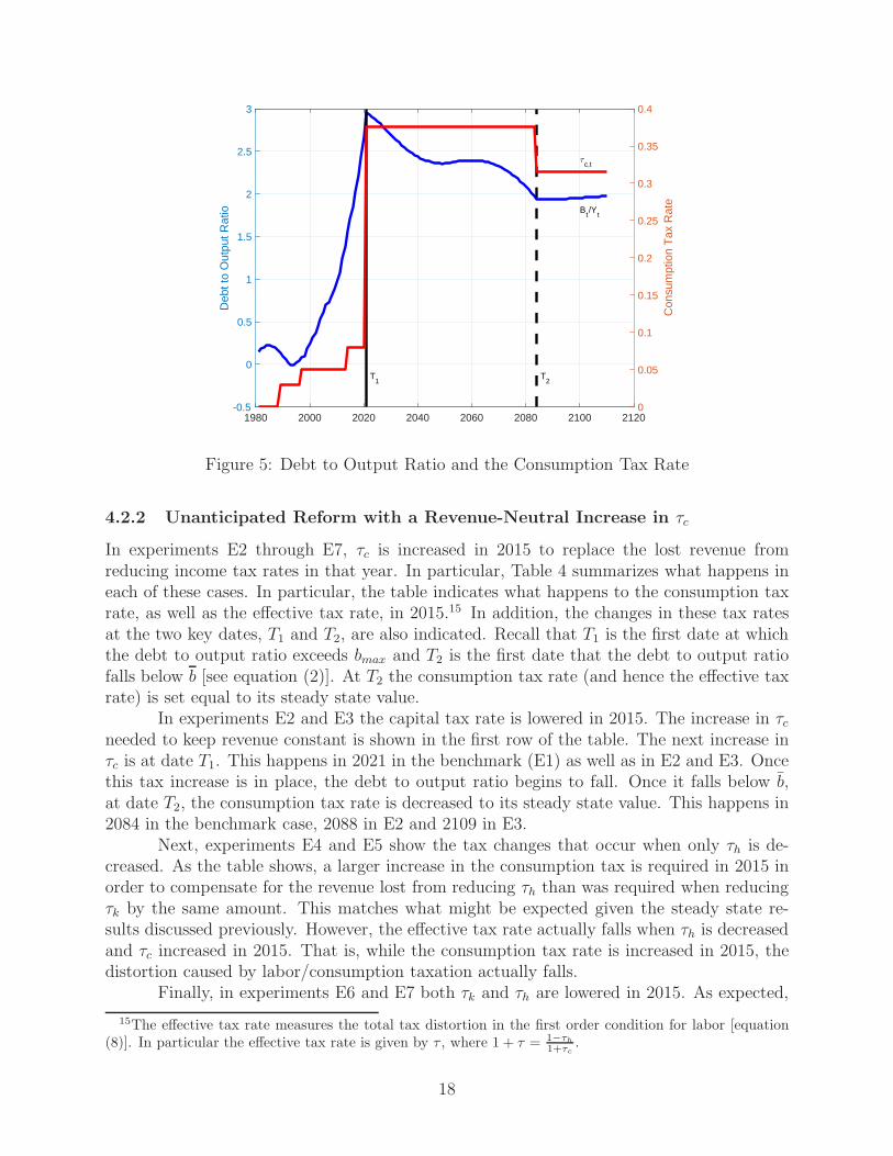
Until 2015, the economy moves along under the expectation that the tax system willnot change except for the use of a higher consumption tax rate when the debt to outputratio exceeds 250%. Figure 5 indicates that the first trigger, T1 occurs in the year 2020 inthis benchmark equilibrium transition E1. The consumption tax rate rises from 8% to 37.6%in order to begin to process of accumulating sufficient tax revenue to pay for the increasingpublic expenditures and to retire a fraction of the outstanding debt toward its steady statelevel. After decades of raising significant revenue, once the public expenditures stabilize in2050 and sufficient debt is retired so that the debt to output is on its path to its steadystate level of 200%, the second trigger occurs in 2084 and the consumption tax rate falls toits steady state level of 31.6%. We can now proceed to describe the short run quantitativefindings in experiments E2 through E7.

17

1980 2000 2020 2040 2060 2080 2100 2120-0.5

0

0.5

1

1.5

2

2.5

3

Deb

t to

Out

put R

atio

0

0.05

0.1

0.15

0.2

0.25

0.3

0.35

0.4

Con

sum

ptio

n T

ax R

ate

T1

T2

Bt/Y

t

c,t

Figure 5: Debt to Output Ratio and the Consumption Tax Rate

4.2.2 Unanticipated Reform with a Revenue-Neutral Increase in τc

In experiments E2 through E7, τc is increased in 2015 to replace the lost revenue fromreducing income tax rates in that year. In particular, Table 4 summarizes what happens ineach of these cases. In particular, the table indicates what happens to the consumption taxrate, as well as the effective tax rate, in 2015.15 In addition, the changes in these tax ratesat the two key dates, T1 and T2, are also indicated. Recall that T1 is the first date at whichthe debt to output ratio exceeds bmax and T2 is the first date that the debt to output ratiofalls below b [see equation (2)]. At T2 the consumption tax rate (and hence the effective taxrate) is set equal to its steady state value.

In experiments E2 and E3 the capital tax rate is lowered in 2015. The increase in τcneeded to keep revenue constant is shown in the first row of the table. The next increase inτc is at date T1. This happens in 2021 in the benchmark (E1) as well as in E2 and E3. Oncethis tax increase is in place, the debt to output ratio begins to fall. Once it falls below b,at date T2, the consumption tax rate is decreased to its steady state value. This happens in2084 in the benchmark case, 2088 in E2 and 2109 in E3.

Next, experiments E4 and E5 show the tax changes that occur when only τh is de-creased. As the table shows, a larger increase in the consumption tax is required in 2015 inorder to compensate for the revenue lost from reducing τh than was required when reducingτk by the same amount. This matches what might be expected given the steady state re-sults discussed previously. However, the effective tax rate actually falls when τh is decreasedand τc increased in 2015. That is, while the consumption tax rate is increased in 2015, thedistortion caused by labor/consumption taxation actually falls.

Finally, in experiments E6 and E7 both τk and τh are lowered in 2015. As expected,

15The effective tax rate measures the total tax distortion in the first order condition for labor [equation(8)]. In particular the effective tax rate is given by τ , where 1 + τ = 1−τh

1+τc.

18

Table 4: Unanticipated Reform with a Revenue-Neutral Increase in τc

E1 E2 E3 E4 E5 E6 E7

τc,2015 0.08 0.1175 0.1708 0.2117 0.4108 0.2493 0.5016τ2015 0.3818 0.4026 0.4298 0.3398 0.2912 0.3596 0.3340T1 2021 2021 2021 2021 2022 2021 2021τc,T1 0.3760 0.3941 0.4238 0.4667 0.6487 0.4985 0.7152τT1 0.5148 0.5211 0.5311 0.4546 0.3935 0.4661 0.4170T2 2084 2088 2109 2100 2106 2078 2141τc,T2 0.3160 0.3241 0.3438 0.4367 0.6287 0.4485 0.6752τT2 0.4927 0.4958 0.5032 0.4432 0.3860 0.4477 0.4031

E1 : Benchmark, τk,t = 0.3409 and τh,t = 0.3324 for all t ≥ 2015

E2 : τk,t = 0.2 and τh,t = 0.3324 for all t ≥ 2015

E3 : τk,t = 0 and τh,t = 0.3324 for all t ≥ 2015

E4 : τk,t = 0.3409 and τh,t = 0.2 for all t ≥ 2015

E5 : τk,t = 0.3409 and τh,t = 0 for all t ≥ 2015

E6 : τk,t = 0.2 and τh,t = 0.2 for all t ≥ 2015

E7 : τk,t = 0 and τh,t = 0 for all t ≥ 2015

T1 : Date when B/Y reaches 250%.

T2 : Date when B/Y is less than or equal to steady state value.

τc,t : Consumption tax rate at date t.

τt = (τc,t + τh,t)/(1 + τc,t) Effective tax rate at date t.

π in equation (2) equals τc,T1− τc,T2

.

the change in τc required in 2015 is larger than in the cases where only one tax rate islowered. In fact, the required increase in experiment E7 (both τk and τh reduced to zero),is equal to the sum of the increases seen in experiments E3 (only τk reduced to zero) andE5 (only τh reduced to zero). In particular, τc is increased by 9.08% in experiment E3, by33.08% in E5, and by 42.16% in E7. A similar results holds for experiments E2, E4 and E6where the tax rates on labor and capital are lowered to 0.2 rather than zero.

The transition paths for the capital stock, hours worked, and output are shown inFigures 6 through 8. In particular, we compare the transitions for the benchmark case (E1),the case where the capital tax rate is set equal to zero in 2015 (E3), the case where the labortax rate is set equal to zero in 2015 (E5) and the case where both tax rates are set equal tozero.

Figure 6 shows that capital stock is slightly above the benchmark path when only τhis set to zero, but is significantly higher when τk is set to zero in experiments E3 and E7.Conversely, hours worked is not much affected by only setting τk equal to zero, as shown inFigure 7, but is increased substantially when τh is set to zero in E5 and E7.

The paths for output, shown in Figure 8, incorporates changes in both inputs toproduction. All policy changes shown increase output relative to the benchmark. Settingboth tax rates to zero (E7) increases output the most while only setting τh to zero (E5)increases it the least.

19

1980 2000 2020 2040 2060 2080 21000

0.5

1

1.5

2

2.5

3

capi

tal

×106

τk = 0.34, τ

h = 0.33 (E1)

τk = 0.00, τ

h = 0.33 (E3)

τk = 0.34, τ

h = 0.00 (E5)

τk = 0.00, τ

h = 0.00 (E7)

Figure 6: Capital Stock

1980 2000 2020 2040 2060 2080 21000.285

0.29

0.295

0.3

0.305

0.31

0.315

0.32

0.325

hour

s w

orke

d

τk = 0.34, τ

h = 0.33 (E1)

τk = 0.00, τ

h = 0.33 (E3)

τk = 0.34, τ

h = 0.00 (E5)

τk = 0.00, τ

h = 0.00 (E7)

Figure 7: Hours Worked

20

1980 2000 2020 2040 2060 2080 21001

2

3

4

5

6

7

8

9

10

outp

ut

×105

τk = 0.34, τ

h = 0.33 (E1)

τk = 0.00, τ

h = 0.33 (E3)

τk = 0.34, τ

h = 0.00 (E5)

τk = 0.00, τ

h = 0.00 (E7)

Figure 8: Output

Table 5: Average Annual Growth Rate of Output per Working Age Population

E1 E3 E5 E7

2015− 2021 0.17% 1.18% 0.61% 1.58%2025− 2060 1.58% 1.62% 1.58% 1.62%

To get a sense for how these policy changes would affect living standards, we showoutput per person in Figure 9. In all cases where income taxation is substituted for consump-tion taxation, the Japanese economy is predicted to enjoy considerable growth in income percapita relative to the benchmark starting in 2015 until date T1 = 2021.16 After 2021, allcases grow at a similar rate, although living standards are permanently higher in the caseswith higher growth beginning in 2015.

The average growth rates for per capita income is shown in Table 5 for the initial yearsafter the policy change (2015-2021) and for the years 2025-2060. In all cases, this growthrate is equal to 1.5% in the balanced growth path to which the model economy ultimatelyconverges. The conclusion to be drawn from this table is that, according to this model,Japan could enjoy considerable growth in the short run by replacing income taxation withconsumption taxation. In fact, the level of output in 2021 is 8.3% higher in experiment E3than in the baseline E1. Similarly, output would be 8.5% higher in E5 and 14.8% higher inE7 when all income taxation is replaced with consumption taxation.

16The value of T1 in E5 is 2022.

21

2015 2020 2025 2030 2035 20405000

5500

6000

6500

7000

7500

8000

per

capi

ta o

utpu

t

τk = 0.34, τ

h = 0.33 (E1)

τk = 0.00, τ

h = 0.33 (E3)

τk = 0.34, τ

h = 0.00 (E5)

τk = 0.00, τ

h = 0.00 (E7)

Figure 9: Output per Person

4.2.3 Unanticipated Reform with a Delayed Increase in τc

In this subsection we consider how our results would change if Japan were to reduce incometax rates in 2015 without increasing τc. Instead, any increase in the consumption tax isdelayed until date T1 and is set according to equation (2). Table 6 provides results fromthe same set of experiments reported on in Table 4. As the first line of this table shows, τcdoes not change from the benchmark in 2015. As a result, T1, the date when the maximumdebt to output ratio is reached, is a year or two earlier than the dates reported in Table 4.The main finding is that the tax increases required at T1 are generally higher than in theprevious case.

22

Table 6: Unanticipated Reform with a Delay in τc

E1 E2 E3 E4 E5 E6 E7

τc,2015 0.08 0.08 0.08 0.08 0.08 0.08 0.08τ2015 0.3818 0.3819 0.3819 0.2593 0.0741 0.2593 0.0741T1 2021 2020 2020 2020 2019 2019 2018τc,T1 0.3760 0.3841 0.4438 0.5067 0.7287 0.5285 0.8052τT1 0.5148 0.5177 0.5376 0.4690 0.4215 0.4766 0.4460T2 2084 2103 2122 2112 2084 2070 2073τc,T2 0.3160 0.3241 0.3438 0.4367 0.6287 0.4485 0.6752τT2 0.4927 0.4958 0.5032 0.4432 0.3860 0.4477 0.4031

E1 : Benchmark, τk,t = 0.3409 and τh,t = 0.3324 for all t ≥ 2015

E2 : τk,t = 0.2 and τh,t = 0.3324 for all t ≥ 2015

E3 : τk,t = 0 and τh,t = 0.3324 for all t ≥ 2015

E4 : τk,t = 0.3409 and τh,t = 0.2 for all t ≥ 2015

E5 : τk,t = 0.3409 and τh,t = 0 for all t ≥ 2015

E6 : τk,t = 0.2 and τh,t = 0.2 for all t ≥ 2015

E7 : τk,t = 0 and τh,t = 0 for all t ≥ 2015

T1 : Date when B/Y reaches 250%.

T2 : Date when B/Y is less than or equal to steady state value.

τc,t : Consumption tax rate at date t.

τt = (τc,t + τh,t)/(1 + τc,t) Effective tax rate at date t.

π in equation (2) equals τc,T1− τc,T2

.

2015 2020 2025 2030 2035 20405000

5500

6000

6500

7000

7500

8000

per

capi

ta o

utpu

t

τk = 0.34, τ

h = 0.33 (E1)

τk = 0.00, τ

h = 0.33 (E3)

τk = 0.34, τ

h = 0.00 (E5)

τk = 0.00, τ

h = 0.00 (E7)

Figure 10: Output per Person

23

Table 7: Average Annual Growth Rate of Output per Working Age Population

E1 E3 E5 E7

2015− 2021 0.17% 0.93% −0.30% 0.80%2025− 2060 1.58% 1.64% 1.64% 1.67%

As can be seen from Table 7 and Figure 10, the growth benefits from tax reform arelower than in the case where the consumption tax rate is increased simultaneously with thereduction in income tax rates. In particular, output in 2021 in experiment E3 is 7.1% higherthan in the baseline (E1). In experiment E5, where only the labor tax is eliminated, outputwould be only 2% higher in 2021. In fact, as can be seen in both Table 7 and Figure 10, thegrowth rate of output per capita is negative in several of the years between 2015 and 2021.If all income taxes are eliminated, output would be 11.3% higher than in the baseline. Thesegrowth rates are lower here relative to the revenue neutral case because lower income taxeswith knowledge that the consumption tax will be raised in the future leads to a temporaryconsumption boom that dampens the investment boom that these tax reforms otherwisetrigger.

4.3 Welfare Analysis

In this section we compute welfare differences across experiments E1-E7. For each experimentE2-E7, we calculate the consumption equivalent variation (CEV) relative to our baselineexperiment by calculating the percent change in consumption that would be required eachperiod in experiment E1 to make the present discounted utility the same as in the alternativeexperiment.

To be more specific, let the realized discounted 1981 value of utility in experimentE1 be denoted by W . This can be calculated using the sequence of consumption, hours andbond holdings that are realized in experiment E1:

W =

∞∑

t=1981

βtNt

[log Ct − α

h1+1/ψt

1 + 1/ψ+ φ log(µt + Bt+1)

].

Let W be the corresponding realized utility for one of our alternative experiments.The CEV, λ, is the percentage change in consumption required in each period so that theaugmented sequence realized in the benchmark transition E1 provides discounted utilityequal to W . That is, λ solves the following equation:

W =

∞∑

t=1981

βtNt

[log[(1 + λ)Ct

]− α

h1+1/ψt

1 + 1/ψ+ φ log(µt + Bt+1)

].

24

Solving for λ yields

λ = exp

(W − W∑∞

t=1981 βtNt

)− 1.

Table 8: Welfare Analysis: CEV (λ) Relative to Experiment 1

For t ≥ 2015 λ λτk,t τh,t (R-neutral) (delay)

E1 0.3409 0.3324 − −E2 0.20 0.3324 0.0090 0.0099E3 0.0 0.3324 0.0196 0.0257E4 0.3409 0.20 0.0047 0.0138E5 0.3409 0.0 0.0111 0.0212E6 0.20 0.20 0.0120 0.0144E7 0.0 0.0 0.0309 0.0362

In Table 8 we report the welfare gains associated with the transition paths for eachexperiment relative to our benchmark, E1. In particular, the fourth and fifth columns of thetable provide the value of λ for each of experiments we have considered. Three patterns fromthis table are worth noting. First, the welfare gains are strictly higher in each experiment ifthe consumption tax increase is delayed until the fiscal trigger is activated (date T1). Thisreflects the role of discounting and may also reflect that, if the increase in τc is delayed, itis anticipated when the unanticipated tax reform is introduced in 2015. An implication ofthis may be that to delay planned consumption tax increases in spite of reducing tax rateson capital income, as Japan has done twice, is not problematic from the perspective of ourmodel.

The second pattern is that the welfare gains from reducing τk are generally largerthan those from reducing τh. For example, in the revenue neutral case, the welfare gainsfrom reducing τk to 0.2 and leaving τh unchanged (experiment E2) are about twice as largeas the gains from leaving τk unchanged and reducing τh to 0.2 (experiment E4). Finally,significant welfare gains–more than 3%–are possible by eliminating all income taxation infavor of consumption taxation (experiment E7).

25

1980 2000 2020 2040 2060 2080 21001

1.5

2

2.5

3

3.5

4

4.5

5

cons

umpt

ion

105

E1E7 revneutralE7 delay

Figure 11: Consumption

1980 2000 2020 2040 2060 2080 21000.285

0.29

0.295

0.3

0.305

0.31

0.315

0.32

0.325

0.33

0.335

hour

s w

orke

d

E1E7 revneutralE7 delay

Figure 12: Hours Worked

5 Conclusion

Japan’s policymakers have recently reduced the effective corporate income tax rate in aneffort to generate higher investment and output. In this paper we use a neoclassical growth

26

model that builds on Hayashi and Prescott (2002), Chen, Imrohoroglu, and Imrohoroglu(2006), and Hansen and Imrohoroglu (2016) to measure the effects of replacing income taxa-tion with consumption taxation on Japan’s economy. Our model is a one sector deterministicgrowth model in which the private sector has perfect foresight about population growth rates,government policy and factor prices. Both the quantity and the price of bonds are endoge-nously determined in our model; government purchases of goods and services and transferpayments are exogenous. The government raises revenue by taxing factor incomes, interestincome and consumption. The representative household values consumption, leisure, andgovernment bonds and markets are complete. By including bonds in the utility function,the model is made consistent with the very strong domestic demand for government bondsin Japan.

Our focus on this paper is an unanticipated tax reform that takes place in 2015.That is, from the beginning (1981), agents in our model anticipate the tax changes thatwill happen when the debt to output ratio reaches the critical level. They do not, however,anticipate the movement away from income taxation that we implement in 2015. We thencompare the welfare and growth consequences of these unanticipated changes relative towhat would happen without such a reform.

We consider two different ways of implementing a policy that reduces income taxesin 2015. First, we assume that the consumption tax rate rises at the beginning of 2015 in or-der to replace the lost revenue associated with the income tax rate reduction; we label theseexperiments ‘revenue-neutral’. In the second set of experiments, no increase in the consump-tion tax is implemented in 2015, which we call ‘delayed increase’ because the governmentis assumed to delay any increase in the consumption tax until the debt to output triggeris reached. Our ‘delayed increase’ experiments seem closer to actual Japanese government’stax reform policy compared to the ‘revenue-neutral’ experiments.17

After calibrating the model to the Japanese economy, we compute transition pathsfrom observed initial conditions in Japan in 1981 to a steady-state in the distant future.Relative to maintaining income tax rates at the 2014 levels, reductions in either the laboror capital income tax (with a higher consumption tax rate to replace lost revenues) producesignificant gains in labor supply or investment in the short run, with the gains higher whenboth income taxes are reduced. These growth effects are larger in the ‘revenue-neutral’experiments.

Our welfare analysis indicates that there are significant gains from reducing incometaxation, more than 3% if all income taxation is eliminated. These welfare gains are generallylarger from reducing the tax on capital income than those from reducing the labor incometax rate.

Finally, the welfare gains are strictly higher in each experiment if the consumptiontax increase is delayed until the fiscal trigger is activated. In other words, our growth effects

17As of September 2017, the actual government policy is close to our ‘delayed increase’ policy in thefollowing two aspects: (i) The increase in the consumption tax rate and the decrease in corporate tax ratehave not gone hand in hand so far. The consumption tax rate was not raised to 10% as scheduled, andthe timing of the rise was postponed, while the corporate tax rate was reduced as scheduled. (ii) The riseof the consumption tax rate and fiscal consolidation going forward explicitly are both committed to by thegovernment. Note also, however, that the actual government policy is different from the ‘delayed increase’policy as it is not explicit in details as to when and how the consolidation is going to be attained.

27

favor the revenue-neutral experiments that call for an immediate rise in the consumption taxrate when income taxation is reduced, but our welfare findings suggest that delaying thisincrease in the consumption tax may be better from the point of view of welfare analysis.This reflects the role of discounting and the fact that even when the consumption tax increaseis delayed it is still fully anticipated to take place in the near future when the unanticipatedtax reform is introduced in 2015.

28

References

Aiyagari, S. R. and E. R. McGrattan (1998). The optimum quantity of debt. Journal ofMonetary Economics 42 (3), 447–469.

Arnold, J. (2008). Do tax structures affect aggregate economic growth? empirical evidencefrom a panel of OECD countries. Working Paper.

Barro, Robert, J. (1990). Government spending in a simple model of endogeneous growth.Journal of Political Economy 98 (55), 103–125.

Buera, F., B. Moll, and Y. Shin (2013). Well-intended policies. Review of Economic Dy-

namics 16 (1), 216–230.

Caballero, R., T. Hoshi, and A. Kashyap (2008). Zombie lending and depressed restruc-turing in japan. American Economic Review 98 (5), 1943–1977.

Chamley, C. (1986). Optimal taxation of capital income in general equilibrium with infinitelives. Econometrica 54 (3), 607–622.

Chen, K., A. Imrohoroglu, and S. Imrohoroglu (2006). The Japanese saving rate. American

Economic Review 96 (5), 1850–1858.

Chetty, R., A. Guren, D. Manoli, and A. W. Broda (2012). Does indivisible labor explainthe the difference between micro and macro elasticities? a meta-analysis of exten-sive margin elasticities. In D. Acemoglu, J. Parker, and M. Woodford (Eds.), NBERMacroeconomics Annual, pp. 1–56. Massachusetts: The University of Chicago Press.

Easterly, W. and S. Rebelo (1993). Fiscal policy and economic growth: An empiricalinvestigation. Journal of Monetary Economics 32 (3), 417–458.

Fukawa, T. and I. Sato (2009). Projection of pension, health and long-term care expen-ditures in Japan through macro simulation. The Japanese Journal of Social Security

Policy 8 (1), 33–42.

Guner, N., G. Ventura, and X. Yi (2008). Macroeconomic implications of size-dependentpolicies. Review of Economic Dynamics 11 (4), 721–744.

Gunji, H. and K. Miyazaki (2011). Estimates of average marginal tax rates on factorincomes in Japan. Journal of the Japanese and International Economies 25 (2), 81–106.

Hansen, G. and S. Imrohoroglu (2016). Fiscal reform and government debt in Japan: Aneoclassical perspective. Review of Economic Dynamics 21 (July), 201–224.

Hayashi, F. and E. C. Prescott (2002). The 1990s in Japan: A lost decade. Review of

Economic Dynamics 5 (1), 206–235.

Hoshi, T. and T. Ito (2014). Defying gravity: Can the Japanese soveriegn debt continueto increase without a crisis? Economic Policy 29 (77), 5–44.

Imrohoroglu, S., S. Kitao, and T. Yamada (2016). Achieving fiscal balance in Japan.International Economic Review 57 (1), 117154.

Judd, K. L. (1985). On the performance of patents. Econometrica 53 (3), 567–586.

29

Knellera, R., M. F. Bleaney, and N. Gemmell (1999). Fiscal policy and growth: evidencefrom OECD countries. Journal of Public Economics 74 (2), 171–190.

Kwon, H. U., F. Narita, and M. Narita (2015). Resource reallocation and zombie lendingin Japan in the 1990s. Review of Economic Dynamics 18 (4), 709–732.

Mendoza, E. G., G. M. Milesi-Ferretti, and P. Asea (1997). On the ineffectiveness of taxpolicy in altering long-run growth: Harberger’s superneutrality conjecture. Journal ofPublic Economics 66 (1), 99–126.

Nakajima, T. and S. Takahashi (2017). Optimum quantity of debt in Japan. UnderstandingPersistent Deflation in Japan Working Paper Series No. 093.

Nutahara, K. (2015). Laffer curves in Japan. Journal of the Japanese and International

Economies 36 (C), 56–72.

Sakuragawa, M. and K. Hosono (2010). Fiscal sustainability of japan: A dynamic stochas-tic general equilibrium approach. The Japanese Economic Review 61 (4), 517–537.

Trabandt, M. and H. Uhlig (2011). The laffer curve revisited. Journal of Monetary Eco-

nomics 58 (4), 305–327.

30