Reinisch_ASD85.515_Chap#7 1 Chapter 7. Atmospheric Oscillations Linear Perturbation Theory To describe large-scale atm ospheric m otions with som e accuracy requires numerical techniques. This makes it difficultto understand the fundam entalprocesses and the balances of forces. Meteorological disturbances often have a wave-like character. Do discuss waves in the atmosphere or in fluids, we linearize the governing equationsusing the perturbation m ethod.

Reinisch_ASD85.515_Chap#71 Chapter 7. Atmospheric Oscillations Linear Perturbation Theory.
Dec 19, 2015
Welcome message from author
This document is posted to help you gain knowledge. Please leave a comment to let me know what you think about it! Share it to your friends and learn new things together.
Transcript

Reinisch_ASD85.515_Chap#7 1
Chapter 7. Atmospheric OscillationsLinear Perturbation Theory
To describe large-scale atmospheric motions with some accuracy requires numerical techniques. This makes it difficult to understand the fundamental processes and the balances of forces. Meteorological disturbances often have a wave-like character. Do discuss waves in the atmosphere or in fluids, we linearize the governing equations using the perturbation method.
Reinisch_ASD85.515_Chap#7 2
7.1 Perturbation Method
1. Field variable = (static portion) + (pertubation portion)
Assume u, v, p, T, etc. are time and longitude-averaged
variables, then ( , ) ' ,u x t u u x t
2. Products of perturbation terms can be neglected.
Example:
' ' ' '' '
u uu u u uu u u u u u
x x x x x

Reinisch_ASD85.515_Chap#7 3
7.2 Properties of WavesWave motions = oscillations in field variables
that propagate in space
Familiar example of oscillation: the pendulum
Equation of motion
sin , restoring force (Fig.7dV
m mgdt
2
2
22 2
2
.1)
, or
0 where (the book uses instead of )
d l d gm mg
dt dt l
d g
dt l

Reinisch_ASD85.515_Chap#7 4
Sinusoidal oscillations and waves
22
2
0
0 0 0
Solution for 0 :
cos sin or cos ,or
= Re Re Re
Re
c s
i t i t i i t
i t
d
dtt t t
e e e e
Ce
A sinusoidal wave propagating in the x direction is given by
, Re where Re is kept in mind.
C= complex amplitude
phase, or
wave number, angular f
c
i kx t i kx t
i
x t Ce Ce
C e
kx t k x tk
k
requency 2 (here f = frequency)f

Reinisch_ASD85.515_Chap#7 5
Phase velocity
How does a point of constant phase move through space?
kx t const
0 0
Phase speed p
D Dxk
Dt DtDx
cDt k
Reinisch_ASD85.515_Chap#7 6
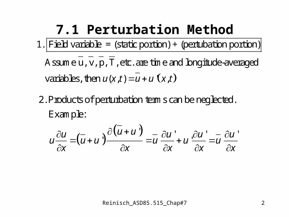
7.21 Fourier SeriesThe wave number k = 2 is defined by the characteristics of the medium
in which the wave propagates. Usually k depends also on the frequency.
Each wave package (disturbance) can be represented as a sum
of waves.
1 1 1
0
01 1
' '1 1 1 10 0 0
1'
1 1
At time t = t 0 :
2sin cos ;
2 2sin sin sin sin sin '
2 2 since sin sin ' 0 for
2
s s s s s s s ss
s s s s ss s
s
xf x A B k x t k x s
x xf x dx A dx A s s dx
x xA s s dx
1
1 1
0
1 10 0
'
2 2sin and cos s s s s
s s
A f x dx B f x dx

Reinisch_ASD85.515_Chap#7 7
7.22 Dispersion and Group VelocityUsually every spectral component propagates with its own phase speed.
This leads to dispersion of a wave package. A wave package consisting of
components around k and propagates with the group velocit y .gc k
1 2 1 2
Derivation: Assume the sum of two waves of equal amplitude, and
, , ,
, exp exp
exp exp exp
, exp cos
k k k k k k
x t i k k x t i k k x t
i kx t i k x t i k x t
x t i kx t k x
g
g
or
, cos cos
2The envelope has a wavelength of . The envelope has a phase
= . Group velocity g
t
x t kx t k x t
k
k x t ck k
Reinisch_ASD85.515_Chap#7 8
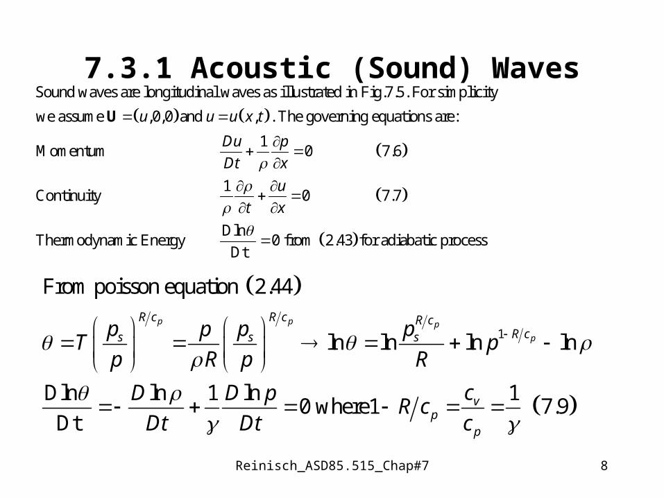
7.3.1 Acoustic (Sound) Waves
Sound waves are longitudinal waves as illustrated in Fig.7.5. For simplicity
we assume ,0,0 and , . The governing equations are:
1Momentum 0 7.6
1Continuity 0 7.7
Thermodynamic En
u u u x t
Du p
Dt x
u
t x
U
Dlnergy 0 from 2.43 for adiabatic process
Dt
1
From poisson equation 2.44
ln ln ln ln
Dln ln 1 ln 10 where1 7.9
Dt
p p p
p
R c R c R cR cs s s
vp
p
p p ppT p
p R p R
cD D pR c
Dt Dt c

Reinisch_ASD85.515_Chap#7 9
Combining 7.7 and 7.9 gives
1 ln0 7.10
Perturbation method:
, ' .
, ' .
, ' .
Neglecting products of primed quatities and considering
that u etc are constant:
D u
Dt x
u x t u u x t
p x t p p x t
x t x t

Reinisch_ASD85.515_Chap#7 10
2 2 2
2
1 '' 0 7.12
t
'' 0 7.13
t
Eliminate ' by applying on 7.13 , and inserting 7.12 :t
''t
' ' 0t t
pu u
x x
uu p p
x x
u ux
u up px
u p p u px x x x

Reinisch_ASD85.515_Chap#7 11
2 2
2
2 2 2 2 22
2 2
22
2
'' 0 7.14
t
Try the following solution:
' exp
' 2 ' 't t t
''
For ' exp to be a solution requ
p pu p
x x
p A ik x ct
u p u u p ikc iku px x x
p p pik p
x
p A ik x ct
2 2
ires therefore that
0 Dispersion relationp
ikc iku ik
pc u u RT

Reinisch_ASD85.515_Chap#7 12
7.3.2 Shallow-Water Gravity Wave1 2Consider 2-fluid system pictured in Fi. 7.7. Stably stratified if .
Waves may propagate along the interface. Assume incompressibility of
the 2 fluids (this avaoids sound waves). In hydrostatic equi
librium:
- . Differentiate re x:
0, if we assume no horizontal gradient in each fluid.
This means also that the horizontal pressure gradient does not vary
with height:
0
p g z
pg
x z x
p p
x z z
x
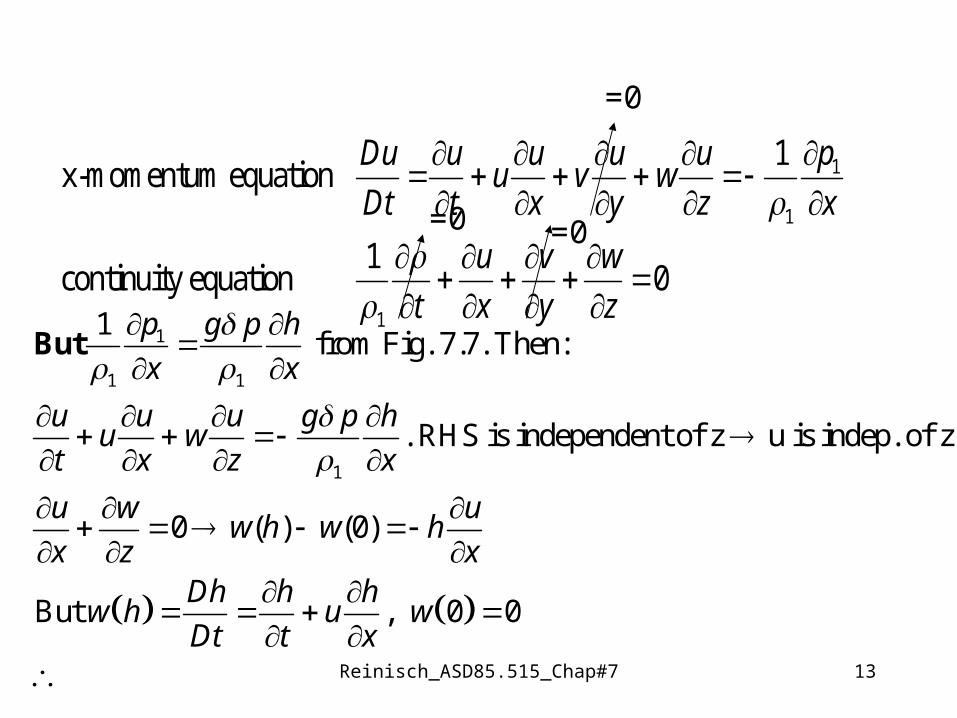
Reinisch_ASD85.515_Chap#7 13
1
1 1
1
1 from Fig. 7.7. Then:
. RHS is independent of z u is indep. of z
0 ( ) (0)
But , 0 0
p g p h
x x
u u u g p hu w
t x z x
u w uw h w h
x z xDh h h
w h u wDt t x
But
1
1
1
1x-momentum equation
1continuity equation 0
pDu u u u uu v w
Dt t x y z x
u v w
t x y z
=0
=0=0

Reinisch_ASD85.515_Chap#7 14
Internal Gravity (or Buoyancy) WavesIn a stably stratified atmosphere gravity waves can propagate. The wave normal
can have horizontal and vertical components, i.e., the wave front (plane of
constant phase) is tilted (Fig.7.8). Vertical
2
22
wave front means horizontal pro-
pagation. In that case the buoancy drives an air parcel vertically up and down as
discussed in section 2.7.3, and the momentum equation is given by 2.52 :
,D
z N z NDt
2 0lndg
dz
22 2
22
2
Assume the wave front is tilted as in Fig. 7.8, then the restoring force is
cos cos cos cos 7.24
The momentum equation becomes now:
cos exp cos ; sinusoidal osci
N z N s N s
Ds N s s A i N t
Dt
llation.

Reinisch_ASD85.515_Chap#7 15
Two-dimensional Internal Gravity Waves
Momentum equation neglecting Coriolis and friction:
D 1
10 7.25
10 7.26
Continuity equation (using Boussinesq approximation):
0 7.27
Energy e
pDt
u u w pu w
t x z x
w u w pu w g
t x z z
u w
x z
Ug
quation:
Dln 1 D0 0 7.28
Dt Dtu w
t x z

Reinisch_ASD85.515_Chap#7 16
Perturbation - Linearization
0
_ _ _
_ _
0
_
0
Poisson equation: 7.29
' (small density perturbance in momentum eq.)
', ', ', ' 7.30
Notice and are functions of height, is not.
p pR c R c
s sp ppT
p R p
u u u w w p p z p z
p
d p z
dz
__ _ _
10_
0
_ _1
0_ _0
and or ln ln ln
7.29 becomes:
' ' 'ln 1 ln 1 ln 1 7.34
pR c
sp z p
g p z constp z
pp const
p

Reinisch_ASD85.515_Chap#7 17
_ _ _
1_ _
0
0 0_ _ _ 2
0
_2
0 0_ 2
' ' 'ln 1 ln ln 1 ln ,
' ' 'Using this in 7.34:
' ' ' '' 7.35
' 'with . But in atmosphere , so
'
s
ss
etc
p
p
p p
cp
pc p RT
c
0_
'. Substitue into linearized 7.25-28 :

Reinisch_ASD85.515_Chap#7 18
_
0
_
_0
__
1 '' 0 7.37
1 ' '' 0 7.38
' '0 7.39
' ' 0 7.40
Eliminate p' from first two by cross differentiation and subtraction:
pu u
t x x
pu w g
t x z
u w
x x
du w
t x dz
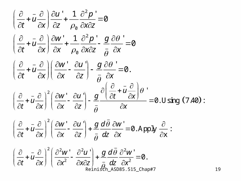
Reinisch_ASD85.515_Chap#7 19
2_
0
2_
_0
_
_
' 1 '0
' 1 ' '0
' ' '0.
u pu
t x z x z
w p gu
t x x x z x
w u gu
t x x z x
_
2_
_
_2_
_
_2 2 2 2_
_2 2
'' '
0. Using 7.40 :
' ' '0. Apply :
x
' ' '0.
uw u g t x
ut x x z x
w u g d wu
t x x z dz x
w u g d wu
t x x x z dz x
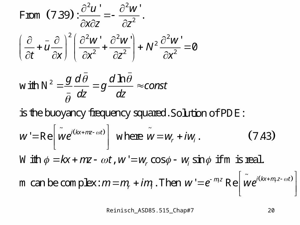
Reinisch_ASD85.515_Chap#7 20
2 2
2
2 2 2 2_2
2 2 2
_ _
2_
' 'From 7.39 : .
' ' '0
lnwith N
is the buoyancy frequency squared.
u w
x z z
w w wu N
t x x z x
g d dg const
dz dz
~ ~
~
Solution of PDE:
' Re where . 7.43
With , ' cos sin if m is real.
m can be complex: . Then ' Re ri
i kx mz tr i
r i
i kx m z tm zr i
w we w w iw
kx mz t w w w
m m im w e we

Reinisch_ASD85.515_Chap#7 21
Dispersion relation
2 2 2 2_2
2 2 2
2_2 2 2 2
_2 2
2 2
Substitute into PDE:
'' 0
0
where
(We assumed here ). "intrinsic frequency".r
wu w N
t x x z x
i u ik k m N k
Nk Nku k k m
k m
m m
κκ
If we define the wave vector , , , then
and
2 , 2 , 2 in our 2-D derivationx y z y
k l m
kx ly mz t
k L l L m L L
κ
κ r κ r

Reinisch_ASD85.515_Chap#7 22
0
0 in Figure
kx mz t const
z k m x const
dz k
dx m
z x
Assume 0, then 0.
The wave vector points downward and eastward. The vertical
wavelength is L 2 , the horizontal wavelength L 2 .
k m
m k
Lz
=kx+mz=const
z
x
Lx

Reinisch_ASD85.515_Chap#7 23
__
_
_
2 2
2 2
The vertical phase speed relative to mean flow is
The horizontal phase speed relative to mean flow is
The phase speed in the direction of ,0, is
Gr
z
x
x z
u kc u
k k
u kc
m
u kk m c c c
k m
κκ
κ
_ _
2 2
2_
3
3
oup velocities:
7.45
7.45
gx
gx
gz
kkk kc u N u Nk
Nmc u a
Nkmc b
m

Reinisch_ASD85.515_Chap#7 24
2 2 2 2 2 2
The tilt angle against the vertical is given by
1cos
1 1
On slide 14, the heuristic gravity frequency was given 7.14 :
cos , i.e. less than the buoyancy frequency N.
cos /
z
x z
L m k k
L L k mk m
N
, i.e. tilt is independent of wave length!N

Reinisch_ASD85.515_Chap#7 25
7.4.2 Topographic Waves
0Air in statically stable conditions d dz 0 flowing over quasi-
sinusoidal mountain ridge is forced to vertical displacements. The
resulting pattern of streamlines is stationary. This means no time
dep
~
2_2 2 2 2
2_2 2 2
endence of soultion, i.e., 0 in 7.43 : ' exp .
Substitute into PDE 7.42 yields the dispersion relation :
0, or
w w i kx mz
u k k m N k
m N u k

Reinisch_ASD85.515_Chap#7 26
2_2 2 2
_2
0
_
_
Discussion: . Assume 0.
0 if . Then m is real,
w'=w cos .
If is a westerly (eastward flow) then the intrinsic frequency 7.44
k 0 (lower sign in 7.44 and
w
m N u k k
Nm u
k
kx mz
u
Nku
,
3
7.45). We associate
a negative frequency with phase propagation in the -z direction, i.e.,
downward. This means 0. The vertical group velocity (7.45b):
0
is upward!
gz
m
c Nkm
Reinisch_ASD85.515_Chap#7 27
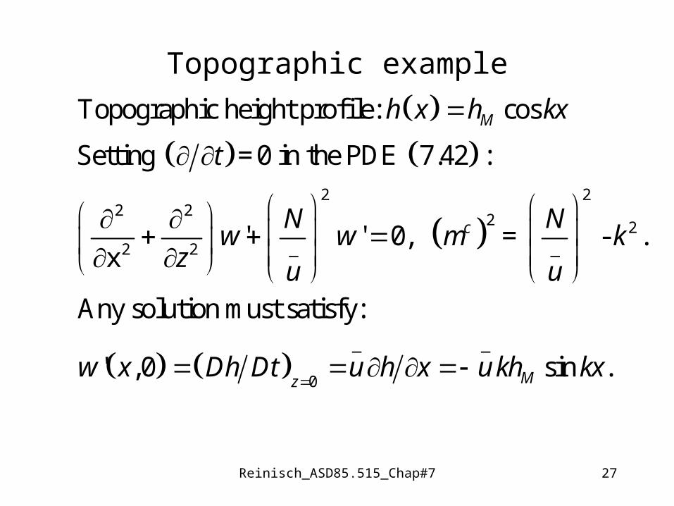
Topographic example
2 22 2
2 22 2 _ _
_ _
0
Topographic height profile: cos
Setting = 0 in the PDE 7.42 :
' ' 0, = - . x
Any solution must satisfy:
' ,0 sin .
M
c
Mz
h x h kx
t
N Nw w m k
z u u
w x Dh Dt u h x u kh kx
Reinisch_ASD85.515_Chap#7 28
_
2 __
2_
_ _
2_22
_
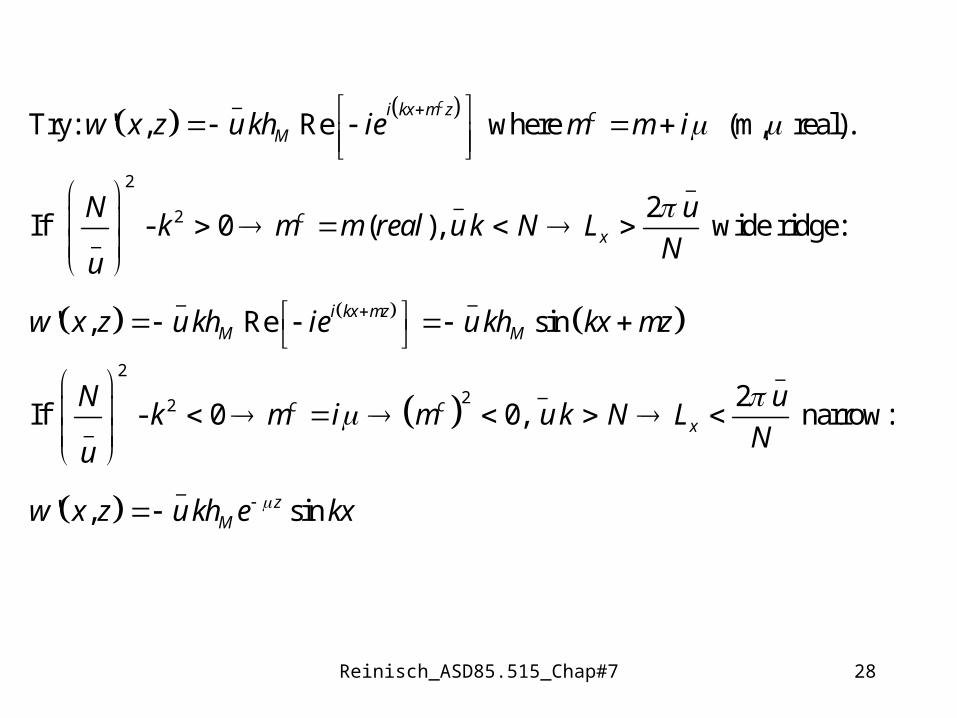
Try: ' , Re where (m, real).
2If - 0 ( ), wide ridge:
' , Re sin
If - 0 0,
ci kx m z cM
cx
i kx mzM M
c c
w x z u kh ie m m i
N uk m m real u k N L
Nu
w x z u kh ie u kh kx mz
Nk m i m u k
u
_
_
2 narrow:
' , sin
x
zM
uN L
N
w x z u kh e kx

Reinisch_ASD85.515_Chap#7 29
7.5.1 Inertial Oscillation
Foe lrager scale gravity waves (few hundred km), Coriolis can no
longer be neglectd, the parcel oscillations are elliptical rather than
straight lines. For simplicity we assume that the parcel motion
2
2
does
not perturb the pressure field. Then from (2.24-25):
17.49
17.50
Leads to ,
Inertial stability for 0
g
g
Du p Dyfv fv f
Dt x Dt
Dv pfu f u u
Dt y
D y Mf y M fy u
Dt y
M

Reinisch_ASD85.515_Chap#7 30
7.5.2 Inertio-gravity Waves
2
We use again the heuristic approach, examining Fig.7.11. Consider an
air parcel oscillating along a slantwise path in the y,z plane. The verical
buoyancy force is cos . The meridional Coriolis foN z
2
22 2
2
2 2 2 2
22 2
2
rce
component is from 7.53 ysin ysin . The
oscillator equation along s becomes
cos ysin
cos sin
cos sin i t
f M y f
D sN z f
Dt
N s f s
D sN f s s e
Dt

Reinisch_ASD85.515_Chap#7 31
2 22
2 8 2 2 20
4
Dispersion relation: cos sin 7.56
Since 10 usually recall ln
, for 0 vertical propagation
110
for 90 horizontal propagation
3
N f
f N f N g d dz
f N N
sff
h

Reinisch_ASD85.515_Chap#7 32
7.7 Rossby Waves
The important waves for large-scale meteorological processes are the
planetary -- or Rossby -- waves. They are a result of the -effect, .
We limit the discussion to free barotropic Rossby wave
df
dy
s. It was shown in
section 4.5 that for a fluid in which =0, the absolute vorticity is
conserved, 0 4.27
0 7.88
since
h
h
D f Dt
u v vt x y
f f f fD f Dt u v v v
t x y y
U
Reinisch_ASD85.515_Chap#7 33
_ _ _
_ _ _
_
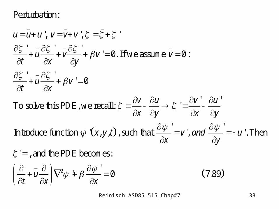
Perturbation:
', ', '
' ' '' 0. If we assume 0 :
' '' 0
' 'To solve this PDE, we recall: '
'Introduce function ' , , , such that
u u u v v v
u v v vt x y
u vt x
v u v u
x y x y
x y t
_
2
'', '. Then
' , and the PDE becomes:
'' 0 7.89
v and ux y
ut x x

Reinisch_ASD85.515_Chap#7 34
2 2 2
_ _2 2 2
_ _2 2
2 2
Try ' exp exp ,
' '
' '
''. This gives the dispersion relation
0 7.91
'' Re ex
i kx ly t i kx ly t
k l
u k l i u ikt x
ikx
kk l u k k u k
k l
u ily
p sin
'' Re exp sin
i kx ly t l kx ly t
v ik i kx ly t k kx ly tx
Reinisch_ASD85.515_Chap#7 35
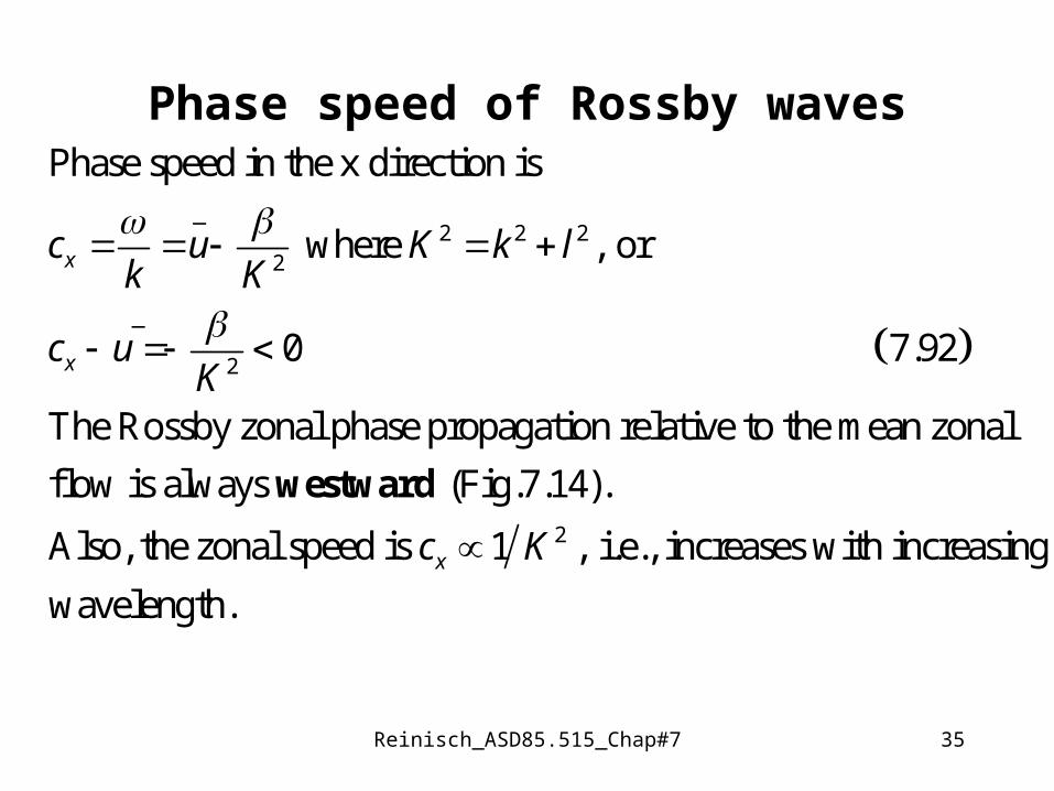
Phase speed of Rossby waves
_2 2 2
2
_
2
Phase speed in the x direction is
where , or
0 7.92
The Rossby zonal phase propagation relative to the mean zonal
flow is always (Fig.7.14).
Also, the zonal speed is
x
x
c u K k lk K
c uK
westward2 1 , i.e., increases with increasing
wavelength.xc K

Reinisch_ASD85.515_Chap#7 36
2 2_
x 2 2 2
2 5 12
2 6
For a typical midlatitude synoptic disturbance with a wavelength of
6000 km and k=l, the Rossby wave speed is
c 2 sin 2 sin2 8 8
7 10 36 10sin ~ c
4 4 6.4 10 10
x x
x
L Ld du
k dy Rd
L d
R d
1
1
_
x
os 45 7
The mean zonal wind speed is generally to the east and larger than
7 . The Rossby wave pattern moves therefore to the east at a
lower speed. If c , the Rossby pattern is stationary re
ms
ms
u
ground.
Related Documents