Reinforcement Learning and Savings Behavior

Electronic copy available at: http://ssrn.com/abstract=1355651

Yale ICF Working Paper No. 09-01

Revised February 2009

Reinforcement Learning and Savings Behavior

James J. Choi School of Management, Yale University National Bureau of Economic Research

David Laibson

Harvard University National Bureau of Economic Research

Brigitte C. Madrian

Harvard University National Bureau of Economic Research

Andrew Metrick

School of Management, Yale University National Bureau of Economic Research

This paper can be downloaded without charge from the Social Science

Electronic copy available at: http://ssrn.com/abstract=1355651

Reinforcement Learning and Savings Behavior

JAMES J. CHOI, DAVID LAIBSON, BRIGITTE C. MADRIAN, and ANDREW METRICK*

Journal of Finance, forthcoming

ABSTRACT

We show that individual investors over­extrapolate from their personal experience

when making savings decisions. Investors who experience particularly rewarding

outcomes from saving in their 401(k)—a high average and/or low variance

return—increase their 401(k) savings rate more than investors who have less

rewarding experiences with saving. This finding is not driven by aggregate time­

series shocks, income effects, rational learning about investing skill, investor

fixed effects, or time­varying investor­level heterogeneity that is correlated with

portfolio allocations to stock, bond, and cash asset classes. We discuss

implications for the equity premium puzzle and interventions aimed at improving

household financial outcomes.

* Choi is at the Yale School of Management and NBER; Laibson is at Harvard University, Department of Economics and NBER; Madrian is at the Harvard Kennedy School and NBER; Metrick is at the Yale School of Management and NBER. This paper is a significantly revised version of a draft that circulated under the title “Consumption­Wealth Comovement of the Wrong Sign.” We thank Hewitt Associates for their help in providing the data. We are particularly grateful to Lori Lucas, Jim McGhee, Scott Peterson, and Yan Xu, some of our many contacts at Hewitt. Outside of Hewitt, we have benefited from the comments of Thomas Knox, Matthew Shapiro, Bill Zame, and seminar participants at Berkeley, Harvard, the NBER Monetary Economics Program Meeting, UCLA, and RAND. We are also indebted to John Beshears, Lucia Chung, Ian Dew­Becker, Keith Ericson, Fuad Faridi, John Friedman, Chris Nosko, Parag Pathak, Nelson Uhan, and Kenneth Weinstein for their excellent research assistance. Financial support from the National Institute on Aging (grants R01­AG021650 and R01­AG16605) is gratefully acknowledged. Choi acknowledges financial support from a National Science Foundation Graduate Research Fellowship, National Institute on Aging Grant T32­AG00186, and the Mustard Seed Foundation. Laibson acknowledges financial support from the National Science Foundation.

Electronic copy available at: http://ssrn.com/abstract=1355651

2

In this paper, we show that individual investors over-extrapolate from their personal return

experience when making savings decisions. Within a given time period, investors who

experience particularly rewarding outcomes from saving in their 401(k)—a high average and/or a

low variance rate of return—increase their 401(k) savings rate more than investors who have less

rewarding experiences with saving.

These effects are economically and statistically significant. All else equal, a one standard

deviation increase in an investor’s 401(k) rate of return during year t increases her 401(k)

savings rate at year-end t by 0.13 percentage points of income. A one standard deviation increase

in the variance of an investor’s 401(k) return during year t lowers her savings rate by 0.16

percentage points at year-end t and 0.34 percentage points at year-end t + 1. By comparison, the

average annual savings rate change in our sample is 0.30 percentage points.

This behavior is not explained by factors that should affect savings rates. We include

controls in our regressions to capture aggregate time fixed effects (such as news about the

macroeconomy or expected asset returns), employer-specific time fixed effects, investor fixed

effects, investor-level income effects, and time-varying investor-level heterogeneity that is

correlated with portfolio allocations to stock, bond, and cash asset classes. Thus, our results

indicate that savings decisions are affected by random accidents of personal financial history that

should not matter to a rational agent.

Our findings are explained by a model in which investors follow a naïve reinforcement-

learning heuristic: increase weights on strategies in which you have personally experienced

success, even if this past success logically does not predict future success. Erev and Roth (1998)

find that a reinforcement-learning model outperforms forward-looking models in predicting how

play evolves in a broad range of economics experiments. Charness and Levin (2003) show that

3

when an (optimal) Bayesian updating rule conflicts with a reinforcement-learning rule,

experimental subjects’ choices shift towards the erroneous option that reinforcement learning

recommends. Our analysis demonstrates that these laboratory learning dynamics also apply to

real-world financial decisions.

The behavior we document also has implications for the equity premium puzzle. If

reinforcement learning exerts an upward force on aggregate savings rates following a positive

equity market return (and the reverse for a negative equity market return), then the time-series

covariance of aggregate consumption growth with equity market returns will be depressed. Choi

(2006) presents a general equilibrium model where investors behave in such a manner. The

model generates volatile equity returns, a high equity Sharpe ratio, and low, stable risk-free rates

that match the historical U.S. data while maintaining smooth aggregate consumption growth and

low investor risk aversion.

Although we do not directly observe the entire savings flow of our 401(k) investors, most

households have few financial assets outside of their 401(k). It is therefore likely that the

changes in the 401(k) savings rate we observe reflect changes in the total savings rate for most of

our sample. When we examine a subset of our sample that has especially strong incentives to

adjust their total savings rate via the 401(k) contribution margin—households whose marginal

401(k) contribution garners a matching contribution from their employer—we continue to find

evidence of return chasing and variance avoidance in the contribution rate.

Our results complement Barber, Odean, and Strahilevetz (2004), who document

brokerage investors’ propensity to repurchase individual stocks they previously sold for a gain

while shunning individual stocks they previously sold for a loss. Barber, Odean and Strahilevetz

find that purchased stocks previously sold for a gain do not subsequently underperform relative

4

to benchmarks based on size and book-to-market. Therefore, conditional on making a purchase,

the propensity to buy previously profitable stocks appears to be welfare-neutral. In our setting,

however, welfare will generally be affected by changes in an employee’s 401(k) contributions,

which are tax-advantaged and often garner a matching employer contribution.

Our results are also related to Kaustia and Knüpfer (2008) and Malmendier and Nagel

(2007). Kaustia and Knüpfer (2008) show that Finnish investors are more likely to subscribe to

future IPOs if they experienced high returns in their prior IPO subscriptions, and posit that this

effect is due to reinforcement learning. Malmendier and Nagel (2007) focus on low-frequency

responses to variation in return experiences across birth cohorts. They show that cohorts that

have experienced high stock market returns throughout their lives hold more stocks, and cohorts

that have experienced high inflation throughout their lives hold fewer bonds. We focus on

higher-frequency responses, and the disaggregated structure of our data allows us to show that

variation in returns within a cohort matters as well.

The rest of the paper proceeds as follows. Section I describes our 401(k) data. Section II

explains the framework within which we conduct our empirical estimation. Section III presents

our results, and Section IV considers alternative interpretations of the results. We conclude in

Section V by reconciling our results with the disposition effect and discussing how our findings

might inform policy interventions intended to improve household financial outcomes.1

I. Data description

Our data come from a large benefits record-keeping firm. We have panel data for five

companies that start when our data provider became the plan administrator at each company and

1 Additional results referenced in the main text are in the Internet Appendix available at http://www.afajof.org/supplements.asp.

5

end at year-end 2000. These data contain the date, amount, and type of every transaction made in

these firms’ 401(k) plans by every participant. In addition, we have year-end cross-sectional

snapshots from 1998, 1999, and 2000 for all active employees that include demographic

information such as their birth date, hire date, gender, compensation, marital status, and state of

residence. The year-end cross-sections also contain point-in-time 401(k) information, including

the contribution rate in effect during the final pay period of the year, total balances, and asset

allocations.

Table I gives summary statistics as of year-end 2000 for our companies, which we code-

name Company A through E. Our sample consists of large firms that span a wide range of

industries. Equally weighting each company, the employees are on average 42.9 years old and

earn $55,292 a year. By comparison, the March 2001 Current Population Survey reports an

average age of 40.8 years and average salary of $45,656 among full-time workers in companies

employing over 1,000 workers and offering some kind of retirement plan. The average 401(k)

participation rate across the firms is 79%, which is close to the 2000 national participation rate of

80% found by the Profit Sharing/401(k) Council of America (2001), and the average balance of

participants is $65,964, which is similar to Holden and VanDerhei’s (2001) reported average

year-end 2000 balance of $61,207 among plans with more than 10,000 participants.

At each of these firms, employees can choose a contribution rate that is an integer

percentage of their salary. The contribution rate determines how much of each paycheck is

deducted and contributed to the plan, and it remains in effect until the employee actively changes

it. All of our companies offer matching contributions proportional to employee contributions up

to a threshold, although Company C did not introduce its match until 2000. For example,

6

employees who contributed at least 3% of their pay at Company B received an additional

contribution from the company equal to 0.75% their pay.

The large majority of the plans’ investment options are mutual funds. Every plan offers at

least eight mutual funds, including at least one fixed-income fund. The most important

investment option that is not a mutual fund is employer stock, which is offered by four of our

five plans. In addition, Companies A and D added a self-directed window to their plans in 2000

and 1999, respectively. Self-directed windows allow participants to buy and sell individual

stocks using their 401(k) balances. We do not observe transactions within the self-directed

windows, although we do know the total balances held in the windows at each year-end. Among

plan participants in Companies A and D, 1.1% and 8.0%, respectively, had any balances in the

self-directed window at year-end 2000. Conditional upon having any money in the window,

participants in Companies A and D held on average 34.1% and 28.1% of their 401(k) balances in

the window, respectively.

All of the plans allow changes to the elected contribution rate and asset allocation on a

daily basis. There is no charge for these changes, which can be made by talking to a benefits

center representative on the phone during business hours, or by using a touch-tone phone system

or the Internet 24 hours a day. With these relatively straightforward methods to make free

changes, the transaction costs seem minimal.

II. Empirical methodology

Our empirical objective is to estimate the relationship between an individual’s 401(k)

contribution rate and the first two moments of 401(k) returns. We compute investor i’s monthly

401(k) returns by weighting each fund’s arithmetic return by the proportion of the portfolio held

7

in the fund at the prior month-end. We then define Ri,t as the arithmetic average of the monthly

401(k) returns in the one-year period t. Ri,t is meant to capture how lucrative an additional

investment in the 401(k) is expected to be if one used only year t’s monthly 401(k) returns to

infer the future 401(k) return-generating process. It does not necessarily reflect the total percent

change in the investor’s wealth during t, which also depends upon the pre-existing 401(k)

balances and the amount and timing of additional contributions to the 401(k). We will control for

total dollar wealth changes later. We define !2(Ri,t) as the variance of the twelve monthly returns

that comprise Ri,t.

We adopt a flexible functional form for the determinants of an individual’s 401(k)

contribution rate. Let Ci,t be the 401(k) contribution rate, measured as a percent of salary, in

effect for individual i at year-end t. Then

2 2, , 1 , 2 , 1 3 , 4 , 1 , ,( ) ( ) ( ) ,i t i i t i t i t i t i t i t i tC g age R R R R" " " ! " ! #$ $% & & & & & &X ! (1)

where gi(·) is a function specific to investor i, agei,t is the investor’s age, Xi,t is a vector of other

control variables defined as of year-end t, and #i,t is the residual term. By using the contribution

rate in effect at year-end rather than the total contributions during the year, we can be sure that

all the information in the explanatory variables was potentially available to the investor before

she made her choice of the dependent variable. The function gi could vary across investors due to

unobserved differences (e.g. discount rates, risk aversion, expected income growth, background

risk) that alter the optimal solution to the lifecycle consumption-investment problem. By

controlling for g, we control for year-over-year contribution changes that would have occurred

regardless of 401(k) returns. We include contemporaneous returns Ri,t and their variance !2(Ri,t)

as explanatory variables. We also include lagged returns and the variance of lagged returns, Ri,t–1

and !2(Ri,t–1), to allow for the possibility of a sluggish response to 401(k) performance. At the

8

end of this section, we discuss and motivate the specific control variables contained in Xi,t for

each of our specifications.

We assume that the function gi(agei,t) is locally well-approximated by a first-order Taylor

expansion around the investor’s age at year-end 1999 (the middle year in our sample of

contribution rates):

, ,1999 , ,1999( ) ( ) ( )2

ii i t i i i t ig age g age age age

'( & $ . (2)

Substituting (2) into (1) and first-differencing yields an equation with an individual fixed

effect in contribution rate changes:

2 2, 1 , 2 , 1 3 , 4 , 1 , ,( ) ( ) .i t i i t i t i t i t i t i tC R R R R' " " " ! " ! #$ $) % & ) & ) & ) & ) & ) & )X ! (3)

We estimate (3) using least-squares regression. We cluster our standard errors at the company ×

state × year level in case peer effects or information spillovers cause dependence in contribution

rate changes between coworkers in the same office (Duflo and Saez (2003), Hong, Kubik, and

Stein (2004), Ivkovich and Weisbenner (2007)).2

Contributions to 401(k) plans are usually made with before-tax money. However, some

of our sample plans allow contributions using after-tax money as well. We add the before-tax

and (if the plan offers the option) after-tax 401(k) contribution rates in effect for the last pay

period of 1998, 1999, or 2000 to calculate Ci,t in each of these years. We include employees

whose contribution rate is zero, provided that they have a positive 401(k) balance.3 We also

require that individuals have salaries greater than $20,000 in 1998 because a large fraction of

2 We estimate the regression by differencing equation (3) to eliminate the investor fixed effect. We cluster standard errors in this double-differenced regression only by company × state, which is equivalent to company × state × year clustering in the first-differenced regression because we observe only two contribution rate changes per person. Consistent with there being only weak geographic effects in contribution rates, our standard errors are barely affected by clustering relative to assuming that all observations are independent. In contrast, the standard errors in our portfolio return persistence analysis, presented in Section IV.A, are greatly increased by clustering.

9

those with salaries under $20,000 are part-time employees who are likely to direct less attention

to the 401(k) than full-time employees.4 In addition, we trim workers who have a one-year

income growth observation greater than 30% or less than –20%, which roughly corresponds to

removing the top 2% and bottom 2% of the income growth distribution. These deleted outliers

are likely caused by transitions between part-time and full-time work status.

The presence of the individual fixed effect imposes the requirement that all employees in

our regressions have two contribution rate change observations. We also need four full years of

capital gains data in order to estimate the coefficients on both contemporaneous and lagged )R

and )!2(R). Thus, our sample is limited to workers who have been actively employed at a

sample firm and continuously enrolled in the 401(k) plan from January 1, 1997 to December 31,

2000. Company E’s data start on March 31, 1997, when our data provider assumed

administrative services for its plan, so we instead require its workers to be actively employed and

continuously enrolled in the plan from March 31, 1997 to December 31, 2000.5

Finally, we drop individuals if their 1998 salary is high enough that, by contributing at

the plan’s maximum before-tax contribution rate, they could exceed the $10,000 statutory limit

on 1998 before-tax 401(k) contributions. The reason we impose this selection rule is that a highly

paid employee could contribute enough that he hits the before-tax dollar limit midway through

the year. For the rest of the year, his before-tax contribution rate is frozen at 0 and does not

reflect his desired contribution rate.6

3 Employees with no balances in the plan are excluded from our analysis because our key explanatory variables, which depend on the individual’s rate of return on plan assets, are only defined for those with assets in the plan. 4 In the March 2001 Current Population Survey, 29.9% of workers who earned less than $20,000 a year worked less than 35 hours a week or fewer than 40 weeks per year. Only 5.6% of workers earning between $20,000 and $30,000 a year satisfied this definition of part-time work. 5 We assign a zero 401(k) return to Company E employees for the first three months of 1997. Our results are qualitatively similar if we drop Company E from the sample. 6 We also drop a small number of Company A employees who are eligible to contribute to the company’s deferred compensation plan.

10

All of our specifications include the log of the employee’s tenure at the company and

company dummies interacted with year dummies in the Xi,t vector. The company × year

dummies control for public news that affects optimal contribution rates in aggregate, as well as

news that is specifically relevant to employees of each company.7

Even after controlling for time shocks common to each company, one might worry that

there is cross-sectional heterogeneity in the time shock that is correlated with 401(k) portfolio

returns. One candidate for such a correlated shock is the wealth effect from the 401(k) portfolio

capital gain itself. Thus, in many specifications, we also control for individual wealth effects by

adding contemporaneous and lagged 401(k) capital gains normalized by current income,

CapitalGaini,t/Yi,t and CapitalGaini,t–1/Yi,t, where CapitalGaini,t is investor i’s 401(k) dollar

capital gain during year t and Yi,t is the investor’s annual salary. We calculate CapitalGaini,t by

taking the difference in balances between year-end t and t – 1 and then subtracting contributions,

rollovers into the plan, and loan repayments during year t and adding back withdrawals and new

loans during year t. We normalize CapitalGain (a variable whose unit is dollars) by income

because the dependent variable in our regressions (contribution rate) is also expressed as a

percent of income.

Another potential concern is that a series of economic news arrived during our sample

period that differentially affected the type of people who tend to hold, say, relatively more

equities (e.g. news about the return to high-skill human capital). Because asset class allocations

are in turn correlated with portfolio returns, this could confound our identification. To account

for this possibility, we will control for interactions between year dummies and three variables:

the dollar amount of the individual’s portfolio held in equities, bonds, and cash at the prior year-

7 Because of the presence of individual fixed effects, we will ultimately be able to identify only one fixed effect per company: the difference between the company’s fixed effect in 2000 and 1999 minus the difference between the

11

end, all as a fraction of current-year income. In our most comprehensive specification, we also

add interactions between year dummies and two variables: the fraction of one’s 401(k) allocated

to equities and to bonds (also at the prior year-end).

Unfortunately, we cannot calculate R and !2(R)—the portfolio percentage return and

variance—including returns in the self-directed windows at Companies A and D, since we do not

observe monthly window balances. The two capital gains variables, however, do include dollar

gains realized in the window. Our contribution rate results are robust to excluding Companies A

and D from the sample.

III. Results

A. Summary statistics

The selection criteria described in Section II leave us with 49,248 contribution rate

change observations on 24,624 employees.8 Table II reports summary statistics for contribution

rate changes and our portfolio return variables. From 1998 to 2000, the median annual

contribution rate change is zero, and the mean change is 0.30 percentage points of income.

Between 1998 and 1999, 20.6% of our sample investors changed their contribution rate, and

22.4% changed their contribution rate between 1999 and 2000 (these specific numbers are not

reported in the table). Over the two years, 35.1% of investors made at least one contribution rate

change.

Pooled across 1997 to 2000, the average monthly 401(k) rate of return, R, has a median

of 0.83% and a mean of 0.99%. Reflecting the dramatic late-1990s bull market and subsequent

company’s fixed effect in 1999 and 1998. 8 At year-end 2000, there were 134,589 active employees at our companies, of whom 100,527 had enrolled in the 401(k), and 69,286 had been enrolled in the 401(k) since at least January 1, 1997 (or March 31, 1997 in the case of Company E). Most of the observations cut from these 69,286 are due to the income cutoff; no employee remaining

12

crash, R has a wide distribution; its pooled cross-sectional standard deviation is 1.41%. The

volatility of monthly portfolio returns, !2(R), also exhibits wide variation across individuals due

to differing portfolio shares allocated to equities and particularly to employer stock. The typical

volatility is quite high, since many plan participants held significant amounts of their employer’s

stock. Our companies’ monthly stock returns generally experienced annualized standard

deviations well over 100% during the sample period. The dollar capital gain normalized by

income, CapitalGain/Y, has an economically narrower range because most investors’ 401(k)

balances are modest compared to their income. The mean and median of CapitalGain/Y are 0.09

and 0.04, respectively, and its standard deviation is 0.30.

B. Main contribution rate regressions

Table III, Panel A presents the coefficients from estimating equation (3) on the full

sample. The first column shows estimates from the baseline specification, which includes first-

differenced contemporaneous and lagged 401(k) return and volatility, log tenure, and company ×

year dummies as explanatory variables. We find that a one standard deviation increase in year t’s

average monthly return causes the 401(k) contribution rate at year-end t to rise by 1.41 × 0.0933

= 0.13 percentage points of income, an effect that is significant at the 1% level. There is no

further increase in year t + 1.

In contrast, a one standard deviation increase in year t volatility causes the contribution

rate at year-end t to fall by 43.80 × 0.0042 = 0.18 percentage points. The contribution rate falls

an additional 0.17 percentage points by year-end t + 1. Both the contemporaneous and lagged

variance-avoidance effects are significant at the 1% level.

in our final sample could exceed the $10,000 statutory limit on 1998 before-tax contributions by contributing at the plan’s maximum contribution rate.

13

To assess the economic significance of these effects, recall that the average annual

contribution rate increase is 0.30 percentage points of income. Thus, the 0.13 percentage point

effect of 401(k) returns and the 0.35 percentage point two-year effect of volatility are substantial

relative to the mean.

Because we are including company × year dummies in our regression, we are controlling

for public news about expected asset returns and news specifically relevant to employees of each

company. Holding fixed news, an investor should not update his beliefs about the future returns

of his 401(k)’s investment options differently based upon how well his own portfolio did. Yet we

find that employees do invest more in their 401(k) when their own portfolio performance was

relatively good. Because we are including individual fixed effects in our regression, we are also

controlling for time-invariant investor heterogeneity—such as risk aversion, time preference,

human capital, etc.—that may affect contribution rates.

Our results are robust to controls for cross-sectional heterogeneity in the time shocks. The

second column of Table III shows that controlling for wealth effects via the contemporaneous

and lagged normalized dollar capital gains in the 401(k) barely affects the coefficients on return

and volatility. The third column of Table III adds controls for the dollar amount held in equities,

bonds, and cash at the prior year-end, and the fourth column adds controls for the fraction of the

401(k) held in equities or bonds at the prior year-end. Even with these additional controls, we

continue to estimate large and statistically significant return chasing and variance avoidance, and

the point estimates remain similar to those in the baseline specification of column 1. In the most

comprehensive specification, we find that a one standard deviation increase in portfolio returns

in year t increases the 401(k) contribution rate in year t by 0.12 percentage points, and a one

standard deviation increase in the volatility of returns in year t decreases the 401(k) contribution

14

rate by 0.16 percentage points at year-end t and by another 0.18 percentage points at year-end t +

1.

We perform several additional robustness checks for our specification. First, we test

whether our results are symmetric. In untabulated regressions, we use splines to allow the return

and variance effects to vary depending on whether the return or variance in a given year is

greater than or less than the prior year’s realization. In every case, we find that the asymmetries

are statistically and economically insignificant. We also find no asymmetry in the return effect

around the S&P 500 benchmark return.

These findings are consistent with individual investors following a naïve reinforcement

learning heuristic: investors expect that investments in which they personally experienced past

rewards will be rewarding in the future, whether or not such a belief is logically justified.

Reinforcement learning models have had success in predicting subject choices in experiments

(Roth and Erev, 1995; Erev and Roth, 1998). Reinforcement learning is often a sensible heuristic

because future rewards are positively correlated with recent rewards in many domains. We show

in Section IV.A that this relationship does not hold true in 401(k) investing.

Do 401(k) contribution rate changes reflect total savings rate changes? We test this by

restricting our sample to participants who at year-end 1998 were contributing less than the

threshold to which their employer would provide matching contributions. These participants face

instantaneous risk-free marginal returns to saving in their 401(k) of 25% to 100%. It is difficult

to imagine that there are alternative investment vehicles that offer comparable risk-adjusted

returns. Therefore, these employees have especially strong incentives to adjust their consumption

expenditures exclusively through their 401(k) contribution rate. Because Company C did not

have a match until 2000, its participants are excluded from this analysis.

15

The results are in Table III, Panel B. The sample restriction causes us to lose 84% of the

sample, which leads to large increases in the standard errors.9 Nevertheless, the coefficients on

the key return and variance variables remain economically large and statistically significant, with

higher (absolute value) point estimates in most cases. Comparing Panels A and B, the coefficient

on )Ri,t increases by an average of about 50% across all four specifications, and the magnitude of

the coefficients on )!2(Ri,t) increase by more than 80%. We conclude that the effect is at least as

strong among these infra-match investors as it is among the whole sample. Since these investors

should be using the 401(k) as their marginal savings vehicle, these results provide evidence that

our findings extend to the broader consumption-savings decision.

C. Interactions with age and salary

A key feature of reinforcement learning models is the “Power Law of Practice”: reactions

to stimuli are large initially and then attenuate as the stock of reinforcements increases and the

marginal stimulus constitutes a smaller proportional addition to the stock (Roth and Erev, 1995).

Reinforcement learning therefore predicts that the contribution rate of young investors is more

responsive to their personal portfolio performance than that of old investors.

The regression in the first column of Table IV tests this prediction by interacting

contemporaneous change in 401(k) return and volatility, )R and )!2(R), with de-meaned

investor age at year-end 1998. Since Table III shows that lagged volatility change also affects

contribution rate changes, we include interactions of this lag with investor age as well. We do not

include the lagged return change, which we found to be insignificant in Table III.10 We

9 We drop the lagged return change variable from Panel B, since it was insignificant in Panel A. Inclusion of that variable here does not qualitatively affect the point estimates, but does increase the standard errors. 10If we include interactions for lagged return changes, then the point estimates on the other coefficients are not qualitatively affected, but there is an increase in the standard errors for the contemporaneous return interactions.

16

acknowledge that age may be a proxy for many different things, so the interactions with age may

be capturing elements other than learning. We interpret our results here with that caveat in mind.

For brevity, we show only the most comprehensive regression specification that controls

for contemporaneous and lagged normalized CapitalGain, asset class balance × year dummies,

and asset class portfolio share × year dummies. We indeed find that both return chasing and

variance avoidance attenuate with age. The age interaction with the contemporaneous change in

401(k) return is significant at the 1% level, as are the age interactions with contemporaneous and

lagged volatility changes, which are both significant at the 1% level and of similar magnitudes.

Each additional decade of age reduces return chasing by 19% and variance avoidance by 30%

relative to the tendencies found in a 21 year old.

Even though responsiveness to portfolio returns decreases with age, investors nonetheless

exhibit reinforcement learning behavior for most of their lives. The point estimates indicate that

return chasing continues until age 74.11 Variance avoidance diminishes more swiftly, but both

contemporaneous and lagged variance-avoidance persists through age 54.

One might suspect that higher-income investors would be less prone to naïve

reinforcement learning, since income is a proxy for financial sophistication. The second column

of Table IV examines whether this is the case by interacting contemporaneous and lagged 401(k)

return change and volatility change with 1998 log salary. Surprisingly, income has no significant

attenuating effect on reinforcement learning tendencies, at least within the low-to-moderate

income investor population in our regressions.

The final column of Table IV interacts return and volatility changes with both age and

log income. We see that the conclusions drawn from the first two columns are robust to allowing

17

this simultaneous interaction. Age continues to attenuate the force of reinforcement learning,

whereas income does not, and the point estimates of the interactions are nearly identical to those

in the first two columns.

IV. Alternative explanations

We now consider alternative mechanisms that could generate the return-chasing and

variance-avoidance results presented above.

A. Learning about investing skill

Investors who experience high 401(k) returns with low variance may be learning that

they have greater skill at 401(k) asset allocation than their coworkers who experience low 401(k)

returns with high variance. Therefore, it may be rational for investors with better performance to

allocate more to their 401(k).12 While the vast majority of research in finance would suggest that

such skill is rare among individual investors,13 it is still useful to perform a direct test in our

sample.

If a high 401(k) return is a sign of high 401(k) investing skill, then we should see

persistence in 401(k) portfolio alphas over time. We regress an investor’s portfolio alpha in year

t on her portfolio alpha in year t – 1, where t = 1998, 1999, and 2000. Three-factor alphas are

11 Age is de-meaned in Table IV to facilitate interpretation of the uninteracted )R and )!2(R) coefficients. The mean age at year-end 1998 in the regression sample is 43.4. Therefore, return chasing drops to zero at age 43.4 + 0.0808/0.0264 × 10 = 74.0 in column 1. 12 Calvet, Campbell, and Sodini (2009) find that investors stop holding both stocks and bonds after realizing poor mutual fund performance. Because Companies A and E do not offer cash as a 401(k) investment option, one may wonder if our performance-chasing results are caused by investors reducing their 401(k) contributions because they simply want to reduce their risky asset share, rather than because they are shying away from 401(k) investing per se. Our contribution rate results are robust to restricting the sample to Companies B, C, and D, which offer cash funds in their 401(k). However, the contemporaneous return-chasing effect (but not the variance-avoidance effects) is more transitory for this subsample: in the most comprehensive regression specification, 71% dissipates in the following year.

18

calculated by regressing monthly excess portfolio returns on the excess market return and the

Fama and French (1993) size and book-to-market factor returns. Four-factor alpha regressions

also include Kenneth French’s momentum factor (MOM) returns. Across our entire sample

period, the average alphas are approximately zero: a portfolio that equally weights participant

portfolios yields a –1 basis point per month (t-statistic = –0.03) three-factor alpha and an 11 basis

point per month (t-statistic = 0.35) four-factor alpha.

We estimate each persistence regression in two different ways: first, using each investor’s

alpha as a linear predictor of his or her subsequent year’s alpha, and second, allowing the

predictive effect of an investor’s alpha to differ depending on whether it is positive or negative.

Investors’ asset allocations are constrained by the investment options offered in their company’s

401(k) plan, so it may be sensible to only compare performance relative to other investors in the

same company. Therefore, we include company × year dummies as explanatory variables.14 We

cluster our regression standard errors by company × year × employee state of residence to

account for the fact that asset allocations (and hence alphas) in our sample may not be

independently chosen within a company locality.

Table V shows the results of these portfolio performance persistence regressions. We see

that, if anything, a good 401(k) portfolio performance this year predicts poor performance the

following year. Three-factor alphas are negatively serially correlated, while the four-factor alpha

exhibits positive serial correlation that is both statistically and economically insignificant. When

we split the alphas into negative and positive cases, we again find no significant evidence of

persistent skill. Under the three-factor model, positive alphas predict lower subsequent alphas,

while under the four-factor model, negative alphas predict higher subsequent alphas.

13 See, for example, Benartzi (2001) for evidence that rank-and-file employees do not have the ability to predict their employer’s stock return.

19

Overall, there is no empirical support for the hypothesis that returns-chasing and

variance-avoidance are driven by rational learning about one’s own investing skill.

B. Rebalancing

There is another potential alternative explanation for our finding that 401(k) contribution

changes are positively related to portfolio returns: if an investor has significant non-401(k)

financial assets, then a positive correlation between 401(k) and non-401(k) asset returns could

produce the appearance of return chasing due to rebalancing. For example, suppose all

households followed a rule of maintaining a fixed dollar amount in non-401(k) assets (a buffer

stock). Then a high 401(k) return would be associated with a high non-401(k) return, which

would cause high-return households to increase 401(k) contributions and increase consumption

out of non-401(k) assets to bring non-401(k) asset values back down to baseline.

This story, however, is inconsistent with some of our other findings. Such a rebalancing

effect should diminish as non-401(k) financial assets get smaller, since the fraction of income

required to restore the non-401(k) balance to its steady-state level diminishes for a given percent

return. Therefore, the rebalancing story predicts that apparent return chasing would be weakest

among the young, who have few financial assets, and strongest among the old. The results

presented above in Section III.C, however, showed that the empirical pattern is exactly the

opposite: return chasing decreases with age.

Furthermore, most 401(k) households have minimal liquid wealth outside of their 401(k)

with which to engage in rebalancing. In the 2001 Survey of Consumer Finances, among 401(k)-

holding households earning between $20,000 and $70,000 a year—a sample roughly comparable

to the one we use in our analysis—the median household has gross non-retirement financial

14 Regressions without company × year fixed effects yield qualitatively similar results on alpha persistence.

20

assets equal to only 2.1 months of income, 76% of which is held in checking, savings, or money

market accounts.15 It is only at the 82nd percentile that households have one year’s income in

gross non-retirement financial assets. These figures probably overstate outside asset holdings in

our sample because the generosity of our 401(k) plans’ early withdrawal and loan provisions

substantially mitigates the need for a precautionary wealth stock outside the 401(k).16

Finally, the rebalancing channel cannot explain the robust variance-avoidance we observe

among our investors.

V. Conclusion

We find that individual investors chase their own historical returns and shy away from

their own historical return variance when making 401(k) savings rate decisions. This behavior

cannot be accounted for by aggregate time fixed effects, employer-specific time fixed effects,

investor fixed effects, investor-level income effects, or time-varying investor-level heterogeneity

that is correlated with portfolio allocations to stock, bond, and cash asset classes. The observed

patterns are consistent with a naïve reinforcement learning heuristic: assets in which one has

personally experienced success are expected to be successful in the future.

These results contrast with the well-documented reluctance to sell assets that have fallen

below their purchase price (Shefrin and Statman, 1985; Odean, 1998), which induces contrarian

trading behavior with respect to one’s personal return history. This “disposition effect” is

15 We count CDs, bonds, savings bonds, publicly traded stock, mutual funds, cash value life insurance, other managed accounts, transactions accounts, and miscellaneous assets as non-retirement financial assets. 16 Table I shows that all of the plans allow participants to take hardship withdrawals from and loans against their 401(k) plan balances, and only one does not allow non-hardship withdrawals. These provisions make 401(k) savings in the companies we study more liquid than for the typical 401(k) participant at the time. The U.S. Department of Labor (2003) reports that in 2000, 40% of full-time employees with savings and thrift plans in private industry were not allowed to take early in-service withdrawals for any reason, and an additional 29% could only take hardship withdrawals. The Profit Sharing/401(k) Council of America (2001) reports that 14% of plans did not permit loans in 2000.

21

anomalous because the asset’s purchase price is investor-specific and already sunk, and hence

should not affect the selling decision in the absence of capital gains taxes.17 The most common

explanation for the disposition effect is that prospect theory preferences (Kahneman and

Tversky, 1979) cause investors to experience disutility from making a sale below the “reference

price” at which they bought the asset (Barberis and Xiong (2008a,b)), and to be risk-seeking for

assets that are mentally classified in the loss domain.

We conjecture that the absence of contrarian behavior in our data is due to two factors.

First, changing one’s ongoing savings rate does not affect whether past investments are

psychologically “booked” as a loss. Second, because the 401(k) investments we observe are

accumulated through periodic asset purchases that are automatically made each payroll period, it

is difficult for the investor to mentally establish a single reference price below which his

investment is in the loss domain. Therefore, the tendency to increase one’s stake in investments

which are underwater is attenuated.

Reinforcement learning is a robust phenomenon because it is often a sensible heuristic;

future rewards are positively correlated with recent rewards in many domains. Our application

may be a rare exception, since we find no evidence that superior performance is persistent. With

the exception of momentum returns over some horizons, the finance literature has found scant

evidence of persistent alphas in public market investing, so we should not expect persistent

alphas among 401(k) participants. Employers and policymakers could try to educate individuals

about this counterintuitive fact. However, financial education is costly and has often been found

to be ineffective (Choi, Laibson, Madrian, and Metrick (2002), Choi, Laibson, and Madrian

(2007, 2008), Cole and Shastry (2007)). Instead, institutional designers may have success in

17 Introducing capital gains taxes should make investors more prone to sell losers (Constantinides (1984)), which is the opposite of what they actually do.

22

mitigating the impact of reinforcement learning by muting the reinforcements themselves,

perhaps by making short-horizon historical performance less salient in disclosure forms and

account statements. Finally, our results provide another argument for programs that provide

prominent (non-zero) defaults for savings levels (Madrian and Shea (2004), Choi, Laibson,

Madrian, and Metrick (2004)) and savings changes (Benartzi and Thaler (2004)). Sensible

defaults combat perverse investment behaviors both by acting as implicit carriers of advice and

by utilizing investor inertia to effect sensible outcomes.

23

REFERENCES

Barber, Brad M., Terrance Odean, and Michal Strahilevitz, 2004, Once Burned, Twice Shy:

Naïve Learning, Counterfactuals, and the Repurchase of Stocks Previously Sold, mimeo,

University of California, Berkeley.

Barberis, Nicholas, and Wei Xiong, 2008a, What Drives the Disposition Effect? An Analysis of

a Long-Standing Preference-Based Explanation, Journal of Finance, forthcoming.

Barberis, Nicholas, and Wei Xiong, 2008b, Realization Utility, mimeo, Yale University.

Benartzi, Shlomo, 2001, Excessive Extrapolation and the Allocation of 401(k) Accounts to

Company Stock, Journal of Finance 56, 1747-1764.

Benartzi, Shlomo, and Richard Thaler, 2004, Save More TomorrowTM: Using behavioral

Economics to Increase Employee Saving, Journal of Political Economy 112, S164-S187.

Calvet, Laurent, John Y. Campbell, and Paolo Sodini, 2009. Fight or Flight? Portfolio

Rebalancing by Individual Investors. Quarterly Journal of Economics 124.

Charness, Gary, and Dan Levin, 2003, When Optimal Choices Feel Wrong: A Laboratory Study

of Bayesian Updating, Complexity, and Affect, American Economic Review 95, 1300-

1309.

Choi, James J., 2006. Extrapolative Expectations and the Equity Premium, mimeo, Yale

University.

Choi, James J., David Laibson, and Brigitte C. Madrian, 2007, $100 Bills on the Sidewalk:

Suboptimal Investment in 401(k) Plans, NBER Working Paper 11554.

24

Choi, James J., David Laibson, and Brigitte C. Madrian, 2008, Why Does the Law of One Price

Fail? An Experiment on Index Mutual Funds, NBER Working Paper 12261.

Choi, James J., David Laibson, Brigitte C. Madrian, and Andrew Metrick, 2002, Defined

Contribution Pensions: Plan Rules, Participant Decisions, and the Path of Least Resistance,

in James Poterba, ed.: Tax Policy and the Economy 16 (MIT Press).

Choi, James J., David Laibson, Brigitte C. Madrian, and Andrew Metrick, 2004, For Better or

For Worse: Default Effects and 401(k) Savings Behavior, in David Wise, ed.: Perspectives

in the Economics of Aging (University of Chicago Press).

Cole, Shawn, and Gauri Kartini Shastry, 2007, If You Are So Smart, Why Aren’t You Rich? The

Effects of Education, Financial Literacy and Cognitive Ability on Financial Market

Participation, mimeo, Harvard Business School.

Constantinides, George M., 1984, Optimal Stock Trading with Personal Taxes: Implications for

Prices and the Abnormal January Returns, Journal of Financial Economics 13, 65-89.

Duflo, Esther, and Emmanuel Saez, 2003, The Role of Information and Social Interactions in

Retirement Plan Decisions: Evidence from a Randomized Experiment, Quarterly Journal

of Economics 118, 815-842.

Erev, Ido, and Alvin E. Roth, 1998, Predicting How People Play Games: Reinforcement

Learning in Experimental Games with Unique, Mixed Strategy Equilibria, American

Economic Review 88, 848-881.

25

Fama, Eugene F., and Kenneth R. French, 1993, Common Risk Factors in the Returns on Stocks

and Bonds, Journal of Financial Economics 33, 3-56.

Holden, Sarah and Jack VanDerhei, 2001, 401(k) plan asset allocation, account balances, and

loan activity in 2000, Investment Company Institute Perspective 7(5), 1-27.

Hong, Harrison, Jeffrey D. Kubik, and Jeremy C. Stein, 2004, Social Interaction and Stock-

Market Participation, Journal of Finance 59, 137-163.

Ivkovich, Zoran, and Scott Weisbenner, 2007, Information Diffusion Effects in Individual

Investors’ Common Stock Purchases: Covet Thy Neighbors’ Investment Choices, Review

of Financial Studies 20, 1327-1357.

Kaustia, Markku, and Samuli Knüpfer, 2008, Do Investors Overweight Personal Experience?

Evidence from IPO Subscriptions, Journal of Finance 63, 2679-2702.

Kahneman, Daniel, and Amos Tversky, 1979, Prospect Theory: An Analysis of Decision Under

Risk, Econometrica 47, 263-291.

Madrian, Brigitte C., and Dennis Shea, 2001, The Power of Suggestion: Inertia in 401(k)

Participation and Savings Behavior, Quarterly Journal of Economics 116, 1149-1187.

Malmendier, Ulrike, and Stefan Nagel, 2007, Depression Babies: Do Macroeconomic

Experiences Affect Risk-Taking?, mimeo, Stanford University.

Odean, Terrance, 1998, Are Investors Reluctant to Realize Their Losses? Journal of Finance 53,

1775-1798.

26

Profit Sharing/401(k) Council of America, 2001, 44th Annual Survey of Profit Sharing and

401(k) Plans (The Council, Chicago).

Roth, Alvin E., and Ido Erev, 1995, Learning in Extensive-Form Games: Experimental Data and

Simple Dynamic Models in the Intermediate Term, Games and Economic Behavior 8, 164-

212.

Shefrin, Hersh, and Meir Statman, 1985, The Disposition to Sell Winners Too Early and Ride

Losers Too Long: Theory and Evidence, Journal of Finance 40, 777-782.

U.S. Department of Labor, Bureau of Labor Statistics, 2003, National Compensation Survey:

Employee Benefits in Private Industry in the United States, 2000.

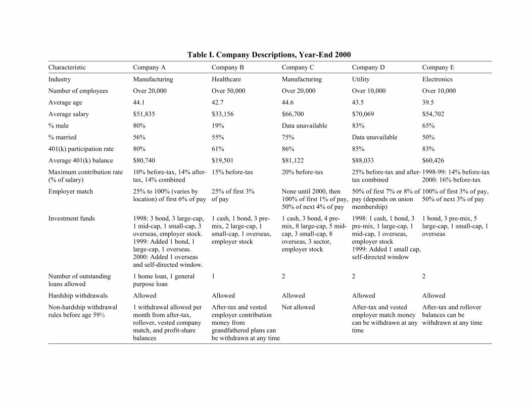
Table I. Company Descriptions, Year-End 2000 Characteristic Company A Company B Company C Company D Company E

Industry Manufacturing Healthcare Manufacturing Utility Electronics

Number of employees Over 20,000 Over 50,000 Over 20,000 Over 10,000 Over 10,000

Average age 44.1 42.7 44.6 43.5 39.5

Average salary $51,835 $33,156 $66,700 $70,069 $54,702

% male 80% 19% Data unavailable 83% 65%

% married 56% 55% 75% Data unavailable 50%

401(k) participation rate 80% 61% 86% 85% 83%

Average 401(k) balance $80,740 $19,501 $81,122 $88,033 $60,426

Maximum contribution rate (% of salary)

10% before-tax, 14% after-tax, 14% combined

15% before-tax 20% before-tax 25% before-tax and after-tax combined

1998-99: 14% before-tax2000: 16% before-tax

Employer match 25% to 100% (varies by location) of first 6% of pay

25% of first 3% of pay

None until 2000, then 100% of first 1% of pay, 50% of next 4% of pay

50% of first 7% or 8% of pay (depends on union membership)

100% of first 3% of pay, 50% of next 3% of pay

Investment funds 1998: 3 bond, 3 large-cap, 1 mid-cap, 1 small-cap, 3 overseas, employer stock. 1999: Added 1 bond, 1 large-cap, 1 overseas. 2000: Added 1 overseas and self-directed window.

1 cash, 1 bond, 3 pre-mix, 2 large-cap, 1 small-cap, 1 overseas, employer stock

1 cash, 3 bond, 4 pre-mix, 8 large-cap, 5 mid-cap, 3 small-cap, 8 overseas, 3 sector, employer stock

1998: 1 cash, 1 bond, 3 pre-mix, 1 large-cap, 1 mid-cap, 1 overseas, employer stock 1999: Added 1 small cap, self-directed window

1 bond, 3 pre-mix, 5 large-cap, 1 small-cap, 1 overseas

Number of outstanding loans allowed

1 home loan, 1 general purpose loan

1 2 2 2

Hardship withdrawals Allowed Allowed Allowed Allowed Allowed Non-hardship withdrawal rules before age 59½

1 withdrawal allowed per month from after-tax, rollover, vested company match, and profit-share balances

After-tax and vested employer contribution money from grandfathered plans can be withdrawn at any time

Not allowed After-tax and vested employer match money can be withdrawn at any time

After-tax and rollover balances can be withdrawn at any time

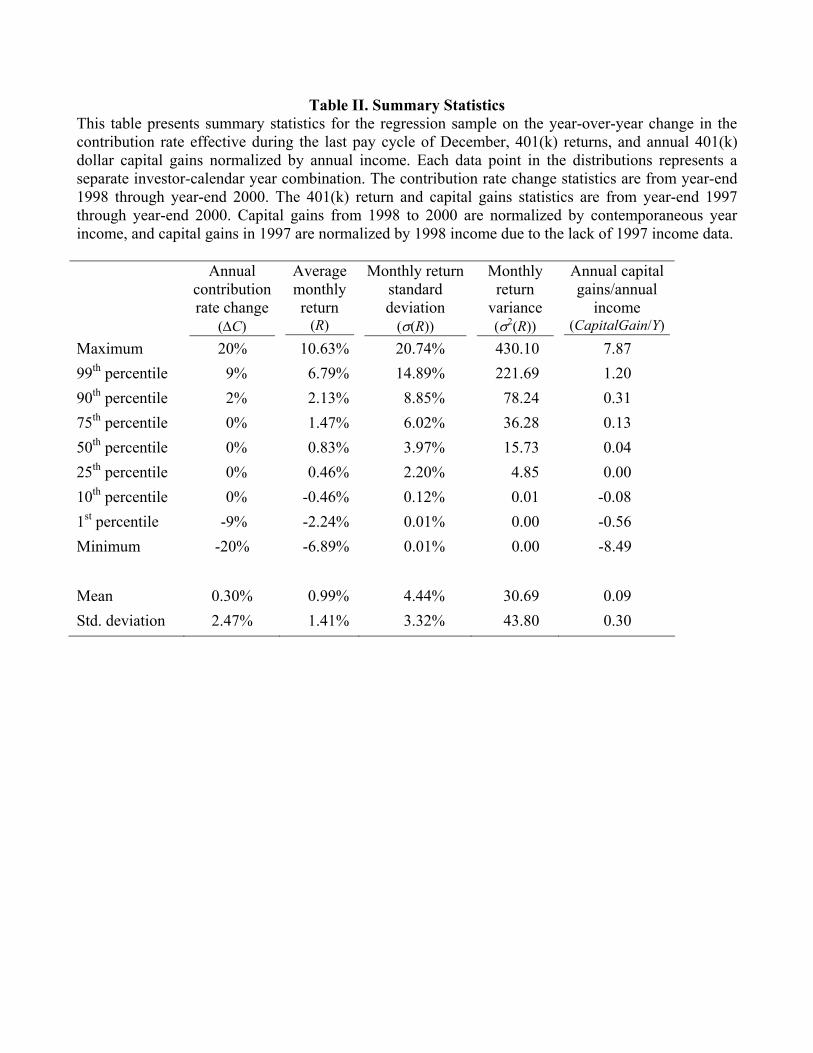
Table II. Summary Statistics This table presents summary statistics for the regression sample on the year-over-year change in the contribution rate effective during the last pay cycle of December, 401(k) returns, and annual 401(k) dollar capital gains normalized by annual income. Each data point in the distributions represents a separate investor-calendar year combination. The contribution rate change statistics are from year-end 1998 through year-end 2000. The 401(k) return and capital gains statistics are from year-end 1997 through year-end 2000. Capital gains from 1998 to 2000 are normalized by contemporaneous year income, and capital gains in 1997 are normalized by 1998 income due to the lack of 1997 income data. Annual

contribution rate change

()C)

Average monthly return

(R)

Monthly return standard deviation

(!(R))

Monthly return

variance (!*(R))

Annual capital gains/annual

income (CapitalGain/Y)

Maximum 20% 10.63% 20.74% 430.10 7.87 99th percentile 9% 6.79% 14.89% 221.69 1.20 90th percentile 2% 2.13% 8.85% 78.24 0.31 75th percentile 0% 1.47% 6.02% 36.28 0.13 50th percentile 0% 0.83% 3.97% 15.73 0.04 25th percentile 0% 0.46% 2.20% 4.85 0.00 10th percentile 0% -0.46% 0.12% 0.01 -0.08 1st percentile -9% -2.24% 0.01% 0.00 -0.56 Minimum -20% -6.89% 0.01% 0.00 -8.49 Mean 0.30% 0.99% 4.44% 30.69 0.09 Std. deviation 2.47% 1.41% 3.32% 43.80 0.30

Table III. Regressions of Contribution Rate Changes on Portfolio Returns and Variance This table presents coefficients from estimating regression equation (3). Panel A contains results for the full sample, and Panel B restricts the sample to those whose contribution rate at year-end 1998 was below the match threshold. The dependent variable is the year-over-year change, in 1999 and 2000, in the contribution rate effective during the last pay cycle of December. The ) operator is for year-over-year changes. The subscript i indexes investors, and t indexes years. Ri,t is average monthly 401(k) percent return, !2(Ri,t) is 401(k) monthly return variance, CapitalGaini,t is 401(k) dollar capital gain, Yi,t is annual salary, and Tenurei,t is the number of years since original hire at the end of year t. The last three table rows indicate whether the regression includes company × year dummies, asset class (equities, bonds, or cash) balances at the prior year-end normalized by income interacted with year dummies, and the share of the 401(k) in equities or bonds at the prior year-end interacted with year dummies. Standard errors, clustered by company × employee’s state of residence in 1998 × year, are in parentheses below the point estimates.

Panel A: Full sample )Ri,t 0.0933** 0.0939** 0.0995** 0.0847** (0.0146) (0.0192) (0.0195) (0.0269) )Ri,t–1 0.0107 -0.0026 -0.0122 -0.0119 + (0.0186) (0.0305) (0.0323) (0.0321) )!2(Ri,t)+ -0.0042** -0.0042** -0.0043** -0.0037** + (0.0009) (0.0009) (0.0010) (0.0009) )!2(Ri,t–1)+ -0.0039** -0.0039** -0.0045* -0.0040* + (0.0014) (0.0015) (0.0018) (0.0017) ),CapitalGaini,t/Yi,t)+ 0.0205 -0.2443* -0.1849+

+ (0.0792) (0.0992) (0.0991) ),CapitalGaini,t–1/Yi,t)+ 0.1833 0.5435+ 0.5727+

+ (0.2165) (0.2960) (0.2946) )Log(Tenurei,t)+ -1.1663 -1.2711 -1.0891 -1.2210 + (0.9470) (0.9965) (0.9756) (0.9942) Company × Year dummies Yes Yes Yes Yes Balance × Year controls No No Yes Yes Share × Year controls No No No Yes N 49,248 49,248 49,248 49,248

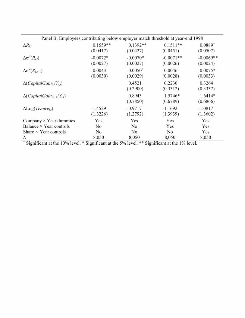
Panel B: Employees contributing below employer match threshold at year-end 1998

)Ri,t 0.1559** 0.1392** 0.1511** 0.0889+ (0.0417) (0.0427) (0.0451) (0.0507) )!2(Ri,t)+ -0.0072* -0.0070* -0.0071** -0.0069** + (0.0027) (0.0027) (0.0026) (0.0024) )!2(Ri,t–1)+ -0.0043 -0.0050+ -0.0046 -0.0075* + (0.0030) (0.0029) (0.0028) (0.0033) ),CapitalGaini,t/Yi,t)+ 0.4521 0.2230 0.3264 + (0.2900) (0.3312) (0.3337) ),CapitalGaini,t–1/Yi,t)+ 0.8943 1.5746* 1.6414* + (0.7850) (0.6789) (0.6866) )Log(Tenurei,t)+ -1.4529 -0.9717 -1.1692 -1.0817 + (1.3226) (1.2792) (1.3939) (1.3602) Company × Year dummies Yes Yes Yes Yes Balance × Year controls No No Yes Yes Share × Year controls No No No Yes N 8,050 8,050 8,050 8,050 + Significant at the 10% level. * Significant at the 5% level. ** Significant at the 1% level.

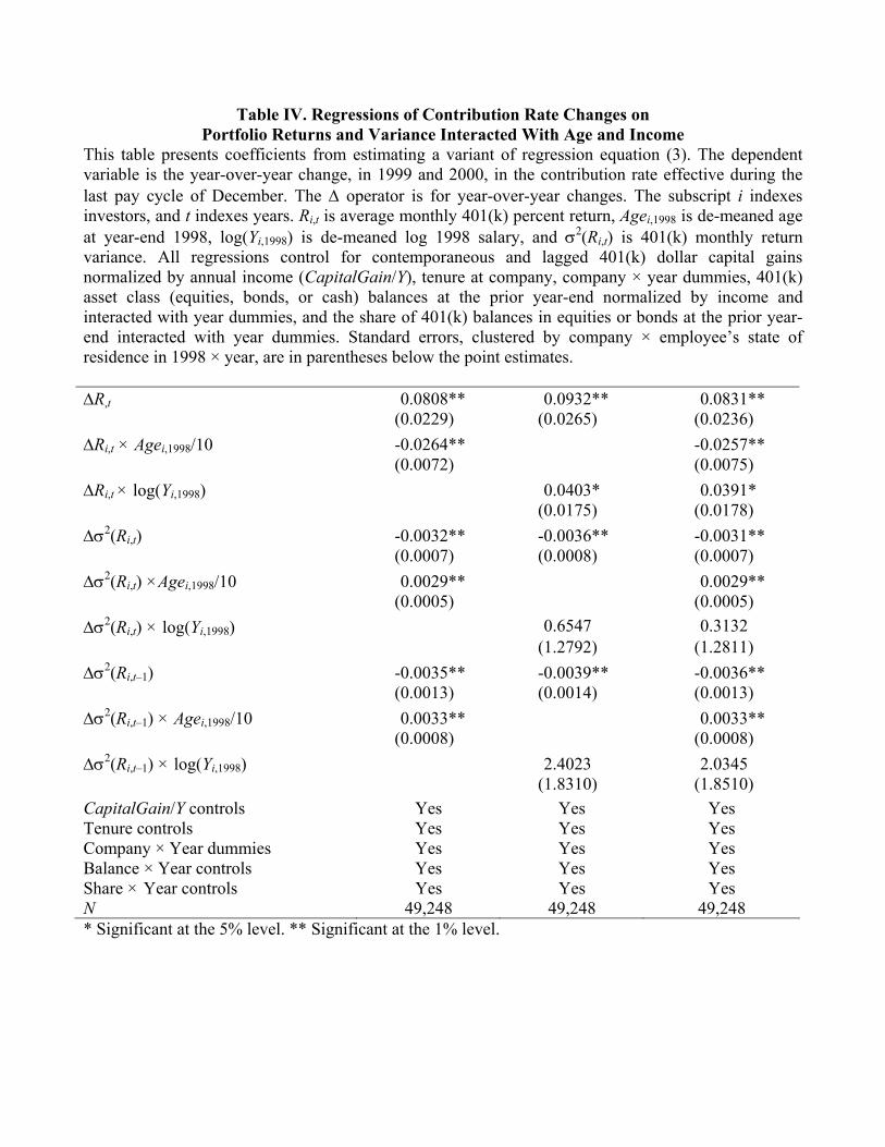
Table IV. Regressions of Contribution Rate Changes on Portfolio Returns and Variance Interacted With Age and Income

This table presents coefficients from estimating a variant of regression equation (3). The dependent variable is the year-over-year change, in 1999 and 2000, in the contribution rate effective during the last pay cycle of December. The ) operator is for year-over-year changes. The subscript i indexes investors, and t indexes years. Ri,t is average monthly 401(k) percent return, Agei,1998 is de-meaned age at year-end 1998, log(Yi,1998) is de-meaned log 1998 salary, and !2(Ri,t) is 401(k) monthly return variance. All regressions control for contemporaneous and lagged 401(k) dollar capital gains normalized by annual income (CapitalGain/Y), tenure at company, company × year dummies, 401(k) asset class (equities, bonds, or cash) balances at the prior year-end normalized by income and interacted with year dummies, and the share of 401(k) balances in equities or bonds at the prior year-end interacted with year dummies. Standard errors, clustered by company × employee’s state of residence in 1998 × year, are in parentheses below the point estimates. )R,t 0.0808** 0.0932** 0.0831** (0.0229) (0.0265) (0.0236) )Ri,t × Agei,1998/10 -0.0264** -0.0257** (0.0072) (0.0075) )Ri,t × log(Yi,1998) 0.0403* 0.0391* (0.0175) (0.0178) )!2(Ri,t)+ -0.0032** -0.0036** -0.0031** + (0.0007) (0.0008) (0.0007) )!2(Ri,t) ×Agei,1998/10+ 0.0029** 0.0029** + (0.0005) (0.0005) )!2(Ri,t) × log(Yi,1998)+ 0.6547 0.3132 + (1.2792) (1.2811) )!2(Ri,t–1)+ -0.0035** -0.0039** -0.0036** + (0.0013) (0.0014) (0.0013) )!2(Ri,t–1) × Agei,1998/10+ 0.0033** 0.0033** + (0.0008) (0.0008) )!2(Ri,t–1) × log(Yi,1998)+ 2.4023 2.0345 + (1.8310) (1.8510) CapitalGain/Y controls Yes Yes Yes Tenure controls Yes Yes Yes Company × Year dummies Yes Yes Yes Balance × Year controls Yes Yes Yes Share × Year controls Yes Yes Yes N 49,248 49,248 49,248 * Significant at the 5% level. ** Significant at the 1% level.

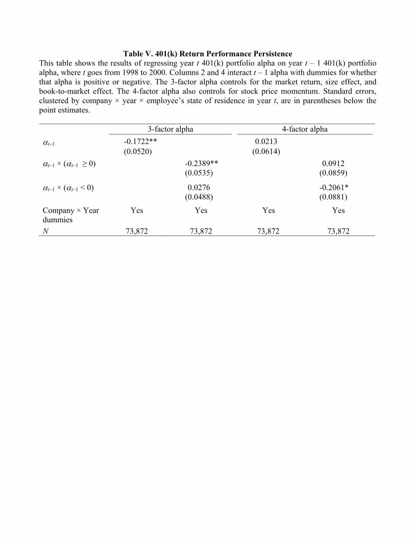
Table V. 401(k) Return Performance Persistence This table shows the results of regressing year t 401(k) portfolio alpha on year t – 1 401(k) portfolio alpha, where t goes from 1998 to 2000. Columns 2 and 4 interact t – 1 alpha with dummies for whether that alpha is positive or negative. The 3-factor alpha controls for the market return, size effect, and book-to-market effect. The 4-factor alpha also controls for stock price momentum. Standard errors, clustered by company × year × employee’s state of residence in year t, are in parentheses below the point estimates. 3-factor alpha 4-factor alpha 't–1 -0.1722** 0.0213 (0.0520) (0.0614) 't–1 × ('t–1 ! 0)+ -0.2389** 0.0912 + (0.0535) (0.0859)

't–1 × ('t–1 < 0) 0.0276 -0.2061* (0.0488) (0.0881)

Company × Year dummies

Yes Yes Yes Yes

N 73,872 73,872 73,872 73,872