Regression analysis

Regression analysis

Developed by

Dr.Ammara Khakwani

Regression:

means “to move backward”,

“Return to an earlier time or stage”

Technically it means

● “The relationship between the mean

value of a random variable and the

corresponding values of one or more

independent variables.”

Formulation of an equation

“The analysis or measure of the

association between one variable

(dependent variable) and one or more

variables ( the independent variable)

usually formulated in an equation in

which the independent variables have

parametric co-efficient which may

enable future values of the dependent

variable to be predicted.”

Regression analysis is concerned

• Regression analysis is largely concerned

with estimating and/or predicting the

(population) mean value of the dependent

variable on the basis of the known or fixed

values of the explanatory variables. The

technique of linear regression is an

extremely flexible method for describing

data. It is a powerful flexible method that

defines much of econometrics. The word

regression, has stuck with us, estimating,

predictive line.

Suppose we want to find out some variables ofinterest Y, is driven by some other variableX. Then we call Y the dependent variable andX the independent variable. In addition,suppose that the relationship between Y andX is basically linear, but is inexact: besides itsdetermination by X, Y has a randomcomponent µ, which we call the ‘disturbance’or ‘error’. The simple linear model is

Y = β1+β2X +µi

Where, β1,β2, are parameters the y-interceptand, the slope of the relationship.

• Helpful for:

• ● Manager making a hiring decision.

• ● Executive can arrive at sales forecasts for a company

• ● Describe relationship between two or more variables

• ● Find out what the future holds before a decision can be made

• ● Predict revenues before a budget can be prepared.

• ● Change in the price of a product and consumer demand for the product.

• ● An economist may want to find out

• ◘ The dependence of personal consumption expenditure on after-tax. It will help him in estimating the marginal propensity to consume, a dollar’s worth of change in real income.

• ● A monopolist who can fix the price or output but not both may want to find out the response of the demand for a product to changes in price.

• A labor economist may want to study, the rate of change of money wages in relation to the unemployment rate.

• ● From monetary Economics, it is known that, other things remaining the same, the higher the rate of inflation (п) the lower the proportion (k) of their income that people would want to hold in the form of money. A quantitative analysis of this relationship will enable the monetary economist to predict the amount to predict the amount of money as a proportion of their income that people would want to hold at various rate of inflation.

Why to study:

• Tools of regression analysis and correlation analysis have been developed to study and measure the statistical relationship that exists between two or more variables.

• ● In regression analysis, an estimating, or predicting, equation is developed to describe the pattern or functional nature of the relationship that exists between the variables.

• ● Analyst prepares an estimating (or regression) equation to make estimates of values of one variable from given values of the others.

• ● Our concern is with predicting

• ◘ The key-idea behind regression analysis is the statistical dependency of one variable, the dependent variable (y) on one or more other variables the independent variables (x).

• ◘ The objective of such analysis is to estimate and predict the (mean) average value of the dependent variable on the basis of the known or fixed values of the explanatory variables

• ◘ The success of regression analysis depends on the availability of the appropriate data.

• ◘ In any research, the researcher should clearly state the source of data used in analysis, their definitions, there method of collection and any gaps or omissions in the data.

• ◘ Its often necessary to prepare a forecast – an explanations of what the future holds before a decision can be made. For example, it may be necessary to predict revenues before a budget can be prepared. These predication become easier if we develop the relationship between the variables to be predict and some other variables relating to it.

• ◘ Computing regression (estimating equation) and then using it to provide an estimate of the value of the dependent variable (response) y when given one or more values of the independent or explanatory variables(s) x.

• ◘ Computing measures that show the possible errors that may be involved in using the estimating equation as a basis for forecasting.

• ◘ Preparing measures that show the closeness or correlation that exists between variables.

What does it provide?

• This method provides an equation

(Model) for estimating; predicting the

average value of dependent variable

(y) from the known values of the

independent variable.

• y is assumed to be random and x are

fixed.

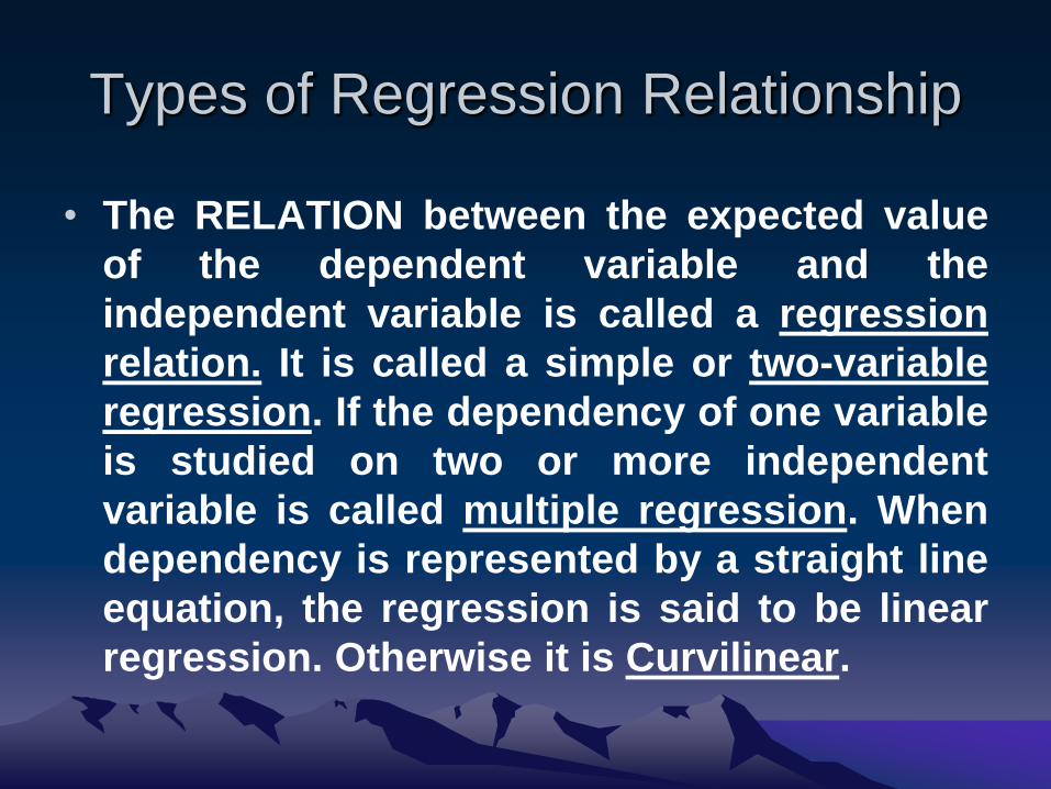
Types of Regression Relationship

• The RELATION between the expected value

of the dependent variable and the

independent variable is called a regression

relation. It is called a simple or two-variable

regression. If the dependency of one variable

is studied on two or more independent

variable is called multiple regression. When

dependency is represented by a straight line

equation, the regression is said to be linear

regression. Otherwise it is Curvilinear.

Example of a model

• Consider a situation where a small ball isbeing tossed up in the air and then we measure itsheights of ascent hi at various moments in time ti.Physics tells us that, ignoring the drag, therelationship can be modeled as

Yi = β1+β2Xi+µi

• where β1 determines the initial velocity of theball, β2 is proportional to the standard gravity,and µI is due to measurement errors. Linearregression can be used to estimate the valuesof β1 and β2 from the measured data. This modelis non-linear in the time variable, but it is linear inthe parameters β1and β2; if we takeregressor xi = (xi1, xi2) = (ti, ti2), the model takeson the standard form

Applications of linear regression

• Linear regression is widely used in

biological, behavioral and social

sciences to describe possible

relationships between variables. It

ranks as one of the most important

tools used in these disciplines.

Correlation:

• In statistics, dependence refers to any

statistical relationship between two random

variables or two sets

of data. Correlation refers to any of a broad

class of statistical relationships involving

dependence. Formally, dependence refers to

any situation in which random variables do

not satisfy a mathematical condition

of probabilistic independence

Pearson correlation coefficient

• In loose usage, correlation can refer to any

departure of two or more random variables

from independence, but technically it refers

to any of several more specialized types of

relationship between mean values. There

are several correlation coefficients, often

denoted ρ or r, measuring the degree of

correlation. The most common of these is

the Pearson correlation coefficient

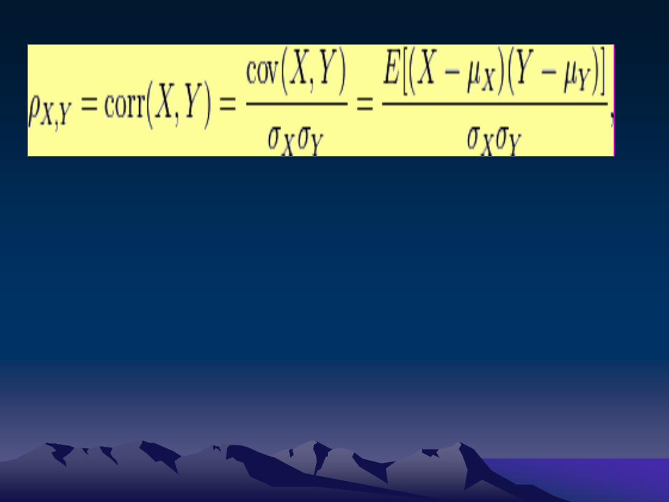
Correlation Coefficient

• The population correlation coefficient ρX,Y between two random variables X and Y with expected valuesμX and μY and standard deviations σX and σY is defined as:

• where E is the expected value operator, cov means covariance, and, corr a widely used alternative notation for Pearson's correlation.

where x and y are the sample means of X and Y,

and sx and sy are the sample standard deviations ofX and Y.

If x and y are results of measurements that contain measurement error,

the realistic limits on the correlation coefficient are not −1 to +1 but a

smaller range

Regression Versus Correlation:

• They are closely related but conceptually different in correlation analysis we measure the strength or degree of linear association between two variables. But in regression analysis we try to estimate or predict the average value of one variable on the basis of the fixed values of other variables. Examples in correlation we can measure the relation between smoking and lung cancer in regression we can predict the average score on a statistics exam by knowing a student score on a mathematical exam.

Regression Versus Correlation:

• They have some fundamental differences. Correlation theory is based on the assumption of randomness of variable and regression theory has assumption that the dependent variable is stochastic and the explanatory variables are fixed or non stochastic. In correlation there is no difference between dependent and explanatory variables.

• In correlation analysis, the purpose is to measure the strength or closeness of the relationship between the variables.

• ♦ What is the pattern of existing relationship

Q, and solution

• The statistical relationship between

the error terms and the regressor

plays an important role in

determining whether an estimation

procedure has desirable sampling

properties such as being unbiased

and consistent.

IMPORTANT TO NOTE

Trend line

• A trend line represents a trend, the long-termmovement in time series data after othercomponents have been accounted for. It tellswhether a particular data set (say GDP, oil pricesor stock prices) have increased or decreased overthe period of time. A trend line could simply bedrawn by eye through a set of data points, butmore properly their position and slope iscalculated using statistical techniques like linearregression. Trend lines typically are straight lines,although some variations use higher degreepolynomials depending on the degree of curvaturedesired in the line.

Trend line uses

• Trend lines are sometimes used in business

analytics to show changes in data over time. Trend

lines are often used to argue that a particular

action or event (such as training, or an advertising

campaign) caused observed changes at a point in

time. This is a simple technique, and does not

require a control group, experimental design, or a

sophisticated analysis technique. However, it

suffers from a lack of scientific validity in cases

where other potential changes can affect the data.

Scatter Diagram:

• To find out whether or not a relationship

between two variables exists, we plot given

data independent and dependent variables

using x-axis for independent regression

variable. Y-axis for dependent variable such

a diagram is called a Scatter Diagram or a

Scatter Plot. If a point shows tendency to a

straight line it is called regression line and if

it shows curve it is called regression curve. It

also shows relationship

GraphScatter Diagram:

Data Graphs:

• Let us assume that a logical

relationship may exist between two

variables.

• To support further analysis we use a

graph to plot the available data. This is

called Scatter Diagram.

• X= Independent or explanatory

• Y= Dependent or response.

Purpose of Diagram:

• To see if there is a useful relationship

between the two variables.

• Determine the type of equation to use

to describe the relationship.

Example of Model Construction:

• Keynes’s consumption function.

• Consumption=C

• Income= X

• C= F(X)

• Consumption and income cannot be connected by any simple deterministic relationship.

• Linear Model

• C= α + β X

• It is hopeless to attempt to capture every influence in the relationship so to incorporate the inherent randomness in the real world counterpart

• C= f(X, ε)

• ε =Stochastic element

• C= α + β X + ε

• Empirical counterpart to Keynes’s theoretical Model.

Example II: Earnings and Education

relationship

• Higher level of education is associated with higher income.

• Simple regression Model is

• Earnings = β1+ β2 education + ε

• [old people have higher income regardless of education]

• And if age and education are positively correlated.

• Han regression Model will associate all the observed increases in education.

• Than with age effects

• Earnings = β1 + β2 education + β3 age + ε

• We also observe than income that income tends to rise less rapidly in the later years than in early so to accommodate this possibility

• Earnings = β1 + β2 education + β3 age + age² + ε

• β3 = +ev

• = -ev

Different ways of linearity

Uses or unique effect of Y• A fitted linear regression model can be

used to identify the relationshipbetween a single predictor variablexj and the response variable y when allthe other predictor variables in themodel are “held fixed”. Specifically, theinterpretation of βj is theexpected change in y for a one-unitchange in xj when the other covariatesare held fixed. This is sometimes calledthe unique effect of x j on y.

Simple and multiple linear

regression

• The very simplest case of a

single scalar predictor variable x and a

single scalar response variable y is

known as simple linear regression.

• The extension to multiple

and/or vector-valued predictor

variables (denoted with a capital X) is

known as multiple linear regression.

General linear models

• The general linear model considers the

situation when the response

variable Y is not a scalar but a vector.

Conditional linearity of E(y|x) = Bx is

still assumed, with a

matrix B replacing the vector β of the

classical linear regression model.

Multivariate analogues of OLS and

GLS have been developed.

Heteroscedasticity models

• Various models have been created that

allow for heteroscedasticity, i.e. the

errors for different response variables

may have different variances. For

example, weighted least squares is a

method for estimating linear regression

models when the response variables may

have different error variances, possibly

with correlated errors.

Generalized linear models

• Generalized linear models (GLM's) are a

framework for modeling a response

variable y that is bounded or discrete.

This is used, for example:

• when modeling positive quantities

• when modeling categorical data

• when modeling ordinal data,

Some common examples of

GLM's are:

• Poisson regression for count data.

• Logistic regression and Probit

regression for binary data.

• Multinomial logistic

regression and multinomial

probit regression for categorical data.

• Ordered probit regression for ordinal

data.

Single index models

• allow some degree of nonlinearity in

the relationship between x and y, while

preserving the central role of the linear

predictor β′x as in the classical linear

regression model. Under certain

conditions, simply applying OLS to

data from a single-index model will

consistently estimate β up to a

proportionality constant.

Hierarchical linear models

• Hierarchical linear models (or multilevelregression) organizes the data into ahierarchy of regressions, for examplewhere A is regressed on B, and B isregressed on C. It is often used where thedata have a natural hierarchical structuresuch as in educational statistics, wherestudents are nested in classrooms,classrooms are nested in schools, andschools are nested in some administrativegrouping such as a school district.

Errors-in-variables

extend the traditional linear regression

model to allow the predictor

variables X to be observed with error.

This error causes standard estimators

of β to become biased. Generally, the

form of bias is an attenuation, meaning

that the effects are biased toward zero.

procedures have been developed

for parameter estimation

• A large number of procedures have beendeveloped for parameter estimation andinference in linear regression. Thesemethods differ in computational simplicityof algorithms, presence of a closed-formsolution, robustness with respect to heavy-tailed distributions, and theoreticalassumptions needed to validate desirablestatistical properties suchas consistency and asymptotic efficiency.

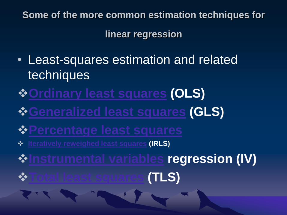
Some of the more common estimation techniques for

linear regression

• Least-squares estimation and related

techniques

Ordinary least squares (OLS)

Generalized least squares (GLS)

Percentage least squares Iteratively reweighed least squares (IRLS)

Instrumental variables regression (IV)

Total least squares (TLS)

Maximum-likelihood estimation and

related techniques

Ridge regression,

Least absolute deviation (LAD)

regression

Adaptive estimation.

Epidemiology

• Early evidence relating tobacco smoking tomortality and morbidity came from observationalstudies employing regression analysis. Forexample, suppose we have a regression model inwhich cigarette smoking is the independentvariable of interest, and the dependent variable islife span measured in years. Researchers mightinclude socio-economic status as an additionalindependent variable, to ensure that any observedeffect of smoking on life span is not due to someeffect of education or income. However, it is neverpossible to include all possible confoundingvariables in an empirical analysis.

Example• For example, a hypothetical gene might increase

mortality and also cause people to smoke more.For this reason, randomized controlled trials areoften able to generate more compelling evidenceof causal relationships than can be obtainedusing regression analyses of observational data.When controlled experiments are not feasible,variants of regression analysis suchas instrumental variables regression may be usedto attempt to estimate causal relationships fromobservational data.

Finance

• The capital asset pricing model uses

linear regression as well as the concept

of Beta for analyzing and quantifying

the systematic risk of an investment.

This comes directly from the Beta

coefficient of the linear regression

model that relates the return on the

investment to the return on all risky

assets.

Economics

• Linear regression is the predominant

empirical tool in economics. For

example, it is used to predict

consumption spending fixed

investment spending, inventory

investment, purchases of a country's

exports spending

on imports the demand to hold liquid

assets labor demand and labor supply

Environmental science

• Linear regression finds application in a

wide range of environmental science

applications. In Canada, the

Environmental Effects Monitoring

Program uses statistical analyses on

fish and benthic surveys to measure the

effects of pulp mill or metal mine

effluent on the aquatic ecosystem

Simple Linear Model:

• The correlation co-efficient may indicate that two variables are associated with one another but it does not give any idea of the kind of relationship involved.

• Hypothesize one variable (Dependent variable) is determined by other variable known as explanatory variables, independent variable or regressor.The hypothesized mathematical relationship linking them is known as the regression model.If there is one regressor, it is described as a simple regression model. If there are two or more regressor it is described as regressor it is described as a multiple regression. We would not expect to find an exact relationship between two economic variables, the relationship is not exact by explicitly including it a random factor known as the disturbance term

Simple Regression Model:

• Yi =β1 + β2Xi +€i

• Has two component β1 , β2Xi

• where β1 and β2 are fixed quantities

known as parameters. The value of

explanatory variable

• the disturbance Ui

yi

yi

Components of model

• Dependent Variable

• is the variable to be estimated. It is plotted on the vertical or y-axis of a chart is therefore identified by the symbol y.

• Independent variable Predictand, regressand, response, explanatory variable,

• is the one that presumably exerts a influence on or explains variations in the dependent variable. It is plotted on x-axis that why denoted by X. It is also called regressor, Predicator regression variable and explanatory variable

We Must Know:

Two Things:

• Value of y-Intercept =a when X is

equal to zero we can read on y-axis.

• Measuring a change of one unit of the

X-variable

• Measuring the Corresponding change

in Yon the y-axis

• Dividing the change inby the change

in X.

Graph

Deterministic and Probabilistic:

• Let us consider a set of n pairs of observations (Xi,Yi). If the relation between the variables is exactly linear, then the mathematical equation describing the linear relation is

• Yi= a+ bYi

• Where, a= value of Y when x=0 , = Intercept

• b= Change in Y for one unit change in X , Slope of line

• It is a deterministic Model.

• C= f(X)

• Consumption function

• Y= a + b X

• (Area = п r²)

• But in some situations it is not exact we get what is called non-deterministic or probabilistic Model.

• = a+ b+ = Unknown Random Errors

Simple Linear regression Model:

• We assume Linear relationship holds between and = α+ β+ = Fixed, Predetermined values

• = Observations drawn from pop

• = Error components

• α, β = Parameters

• α= Intercept

• β= Slope Reg-co-efficient

• β= +ve, -ve based upon the direction of the relationship between X and Y.

• Further more we assume.

• E () =0

• => E(Y) ----------- X is a st. line

• Var () = σ²

• ε ~ N(0, σ²)

• E (,) =0 cov=0

• E(X,) are independent of each other.

Multiple Linear Regression

Model:• It is used to study the relationship between a dependent variable and one or

more independent variables.

• The form of model is

• Y= f (X1+X2+X3+…+Xk) + ε

• = X1 β1 + X2 β2 + X3 β3 +……+ βkXk + ε

• Y= Dependent or explained variable

• X1-------Xk = Independent or Explanatory Variable

• f( X1+X2+X3+…+Xk) = Population regression equation of y on X1-------Xk

• Y= Sum (Deterministic part+ Random Part )

• Y= Regressand

• Xk = Regressors, Covariates

• For example we take a demand equation

• Quantity = β1 + Price× β2 +Income× β3 + ε

• Inverse demand equation

• Price= + × quantity + × income +u

• ε, u = Disturbance, Because it disturb the model.

• Because we cannot hope to capture every influence.

table

What table is showing:

• Output for a time period in dozens of units (Y).

• Aptitude test results for eight employees (X)

• ♦ It is a sample small of 8 emp.

• Q#1 If the test does what is supposed to do.

• Q#2 Employees with higher scores will be among the higher producers.

• ♦ Every point on diagram represents each employees

• C= (X, Y) Pairs of observations

• F= (X, Y)

• ♦ They are making a path in straight line.

• ♦ So there is a linear relationship.

• ♦ (+ev) direct relationship

Ordinary Least Square (OLS):

Estimator:

• Is one of the simplest methods of linear

regression. The goal of OLS is to

closely fit a function with the data. It

does so by minimizing the sum of

squared errors from the data. We are

not trying to minimize the sum of

absolute errors, but rather the sum of

squared errors.

Linear regression model and

assumptions:

1. Model Specification:

2. Homoscedasticity and non-

autocorrelation:

3. 1) Linearity There is no exact linear relationship among any of the

independent variables in the model.

• (Identification Condition)

• Exogeneity of independent variables

From monetary Eco nomics

• it is known that, other things remaining the

same, the higher the rate of inflation (п) the

lower the proportion (k) of their income that

people would want to hold in the form of

money. A quantitative analysis of this

relationship will enable the monetary

economist to predict the amount to predict

the amount of money as a proportion of their

income that people would want to hold at

various rate of inflation.

LS OR OLS:

• The principle of least square consists of determining the values for the unknown parameters that will minimize the sum of squares of errors (or residuals). Where errors are defined as the differences between observed values and the corresponding values predicted or estimated by the fitted model equation.

• The parameters values thus determine will give the least sum of the square of errors and are known as least squares estimates.

• It gives us the least sum of the squares of errors and are known as least squares estimates.

Method of ordinary least square

(OLS):

• It is one of the econometric methods

that can be used to derive estimates of

the parameters of economic

relationships from statistical

observations.

Advantages of OLS

• 1) It is a fairly simple as compared with other econometric techniques.

• 2) This method is used in a wide range of economic relationships.

• 3) It is still one of the most commonly employed methods in estimating relationships in econometric models.

• 4) The mechanics of least square are simple to understand.

• 5) OLS is an essential component of most other econometric techniques.

• 6) Appealing mathematically as compared to other methods.

• 7) It is one of the most powerful and popular methods of regression analysis.

• 8) They can be easily computed.

• 9) They are point estimators. Each estimator will provide only a single (point).

• 10) Once the OLS estimates are obtained from the sample data the sample regression line can be easily obtained.

Model Specification

• Economic study does not specify whether the supply should be studied with a single – equation model or with simultaneous - equation.

• We choose to start our investigation with a single –equation Model.

• Economic theory is not clear about the mathematical form (linear or non linear)

• We start by assuming that the variables are related with the simplest possible mathematical form that the relationship between quantity and price is linear of the form.

• Y= a+ b X

Example:

• Quantity supplied of a commodity and its price.

• When price raises the quantity of the commodity supplied increases

• Step I:

• Specification of the supply model.

• i.e.

• Dependent Variable regressand] = quantity supply

• Explanatory variable regressor] = Price

• Y= f(X)

• Y= β1 + β2 X + [Variation in] = [Explained variation] + [Unexplained Variation]

• β1, β2 = Parameters of supply function our aim is to obtain ,

• = Due to methods of collecting and processing statistical information.

Assumptions

• Weak exogeneity.

• Linearity.

• Constant variance

(aka homoskedasticity

heteroscedasticity

Independence of errors.

Lack of multicollinearity