Examples: Regression And Path Analysis 19 CHAPTER 3 EXAMPLES: REGRESSION AND PATH ANALYSIS Regression analysis with univariate or multivariate dependent variables is a standard procedure for modeling relationships among observed variables. Path analysis allows the simultaneous modeling of several related regression relationships. In path analysis, a variable can be a dependent variable in one relationship and an independent variable in another. These variables are referred to as mediating variables. For both types of analyses, observed dependent variables can be continuous, censored, binary, ordered categorical (ordinal), counts, or combinations of these variable types. In addition, for regression analysis and path analysis for non-mediating variables, observed dependent variables can be unordered categorical (nominal). For continuous dependent variables, linear regression models are used. For censored dependent variables, censored-normal regression models are used, with or without inflation at the censoring point. For binary and ordered categorical dependent variables, probit or logistic regression models are used. Logistic regression for ordered categorical dependent variables uses the proportional odds specification. For unordered categorical dependent variables, multinomial logistic regression models are used. For count dependent variables, Poisson regression models are used, with or without inflation at the zero point. Both maximum likelihood and weighted least squares estimators are available. All regression and path analysis models can be estimated using the following special features: Single or multiple group analysis Missing data Complex survey data Random slopes Linear and non-linear parameter constraints Indirect effects including specific paths Maximum likelihood estimation for all outcome types Bootstrap standard errors and confidence intervals

Welcome message from author
This document is posted to help you gain knowledge. Please leave a comment to let me know what you think about it! Share it to your friends and learn new things together.
Transcript

Examples: Regression And Path Analysis
19
CHAPTER 3
EXAMPLES: REGRESSION AND
PATH ANALYSIS
Regression analysis with univariate or multivariate dependent variables
is a standard procedure for modeling relationships among observed
variables. Path analysis allows the simultaneous modeling of several
related regression relationships. In path analysis, a variable can be a
dependent variable in one relationship and an independent variable in
another. These variables are referred to as mediating variables. For both
types of analyses, observed dependent variables can be continuous,
censored, binary, ordered categorical (ordinal), counts, or combinations
of these variable types. In addition, for regression analysis and path
analysis for non-mediating variables, observed dependent variables can
be unordered categorical (nominal).
For continuous dependent variables, linear regression models are used.
For censored dependent variables, censored-normal regression models
are used, with or without inflation at the censoring point. For binary and
ordered categorical dependent variables, probit or logistic regression
models are used. Logistic regression for ordered categorical dependent
variables uses the proportional odds specification. For unordered
categorical dependent variables, multinomial logistic regression models
are used. For count dependent variables, Poisson regression models are
used, with or without inflation at the zero point. Both maximum
likelihood and weighted least squares estimators are available.
All regression and path analysis models can be estimated using the
following special features:
Single or multiple group analysis
Missing data
Complex survey data
Random slopes
Linear and non-linear parameter constraints
Indirect effects including specific paths
Maximum likelihood estimation for all outcome types
Bootstrap standard errors and confidence intervals

CHAPTER 3
20
Wald chi-square test of parameter equalities
For continuous, censored with weighted least squares estimation, binary,
and ordered categorical (ordinal) outcomes, multiple group analysis is
specified by using the GROUPING option of the VARIABLE command
for individual data or the NGROUPS option of the DATA command for
summary data. For censored with maximum likelihood estimation,
unordered categorical (nominal), and count outcomes, multiple group
analysis is specified using the KNOWNCLASS option of the
VARIABLE command in conjunction with the TYPE=MIXTURE
option of the ANALYSIS command. The default is to estimate the
model under missing data theory using all available data. The
LISTWISE option of the DATA command can be used to delete all
observations from the analysis that have missing values on one or more
of the analysis variables. Corrections to the standard errors and chi-
square test of model fit that take into account stratification, non-
independence of observations, and unequal probability of selection are
obtained by using the TYPE=COMPLEX option of the ANALYSIS
command in conjunction with the STRATIFICATION, CLUSTER, and
WEIGHT options of the VARIABLE command. The
SUBPOPULATION option is used to select observations for an analysis
when a subpopulation (domain) is analyzed. Random slopes are
specified by using the | symbol of the MODEL command in conjunction
with the ON option of the MODEL command. Linear and non-linear
parameter constraints are specified by using the MODEL
CONSTRAINT command. Indirect effects are specified by using the
MODEL INDIRECT command. Maximum likelihood estimation is
specified by using the ESTIMATOR option of the ANALYSIS
command. Bootstrap standard errors are obtained by using the
BOOTSTRAP option of the ANALYSIS command. Bootstrap
confidence intervals are obtained by using the BOOTSTRAP option of
the ANALYSIS command in conjunction with the CINTERVAL option
of the OUTPUT command. The MODEL TEST command is used to test
linear restrictions on the parameters in the MODEL and MODEL
CONSTRAINT commands using the Wald chi-square test.
Graphical displays of observed data and analysis results can be obtained
using the PLOT command in conjunction with a post-processing
graphics module. The PLOT command provides histograms,
scatterplots, plots of individual observed and estimated values, and plots
of sample and estimated means and proportions/probabilities. These are

Examples: Regression And Path Analysis
21
available for the total sample, by group, by class, and adjusted for
covariates. The PLOT command includes a display showing a set of
descriptive statistics for each variable. The graphical displays can be
edited and exported as a DIB, EMF, or JPEG file. In addition, the data
for each graphical display can be saved in an external file for use by
another graphics program.
Following is the set of regression examples included in this chapter:
3.1: Linear regression
3.2: Censored regression
3.3: Censored-inflated regression
3.4: Probit regression
3.5: Logistic regression
3.6: Multinomial logistic regression
3.7: Poisson regression
3.8: Zero-inflated Poisson and negative binomial regression
3.9: Random coefficient regression
3.10: Non-linear constraint on the logit parameters of an unordered
categorical (nominal) variable
Following is the set of path analysis examples included in this chapter:
3.11: Path analysis with continuous dependent variables
3.12: Path analysis with categorical dependent variables
3.13: Path analysis with categorical dependent variables using the
Theta parameterization
3.14: Path analysis with a combination of continuous and
categorical dependent variables
3.15: Path analysis with a combination of censored, categorical, and
unordered categorical (nominal) dependent variables
3.16: Path analysis with continuous dependent variables,
bootstrapped standard errors, indirect effects, and confidence
intervals
3.17: Path analysis with a categorical dependent variable and a
continuous mediating variable with missing data*
3.18: Moderated mediation with a plot of the indirect effect

CHAPTER 3
22
* Example uses numerical integration in the estimation of the model.
This can be computationally demanding depending on the size of the
problem.
EXAMPLE 3.1: LINEAR REGRESSION
TITLE: this is an example of a linear regression
for a continuous observed dependent
variable with two covariates
DATA: FILE IS ex3.1.dat;
VARIABLE: NAMES ARE y1-y6 x1-x4;
USEVARIABLES ARE y1 x1 x3;
MODEL: y1 ON x1 x3;
In this example, a linear regression is estimated.
TITLE: this is an example of a linear regression
for a continuous observed dependent
variable with two covariates
The TITLE command is used to provide a title for the analysis. The title
is printed in the output just before the Summary of Analysis.
DATA: FILE IS ex3.1.dat;
The DATA command is used to provide information about the data set
to be analyzed. The FILE option is used to specify the name of the file
that contains the data to be analyzed, ex3.1.dat. Because the data set is
in free format, the default, a FORMAT statement is not required.
VARIABLE: NAMES ARE y1-y6 x1-x4;
USEVARIABLES ARE y1 x1 x3;
The VARIABLE command is used to provide information about the
variables in the data set to be analyzed. The NAMES option is used to
assign names to the variables in the data set. The data set in this
example contains ten variables: y1, y2, y3, y4, y5, y6, x1, x2, x3, and
x4. Note that the hyphen can be used as a convenience feature in order
to generate a list of names. If not all of the variables in the data set are
used in the analysis, the USEVARIABLES option can be used to select a
subset of variables for analysis. Here the variables y1, x1, and x3 have

Examples: Regression And Path Analysis
23
been selected for analysis. Because the scale of the dependent variable
is not specified, it is assumed to be continuous.
MODEL: y1 ON x1 x3;
The MODEL command is used to describe the model to be estimated.
The ON statement describes the linear regression of y1 on the covariates
x1 and x3. It is not necessary to refer to the means, variances, and
covariances among the x variables in the MODEL command because the
parameters of the x variables are not part of the model estimation.
Because the model does not impose restrictions on the parameters of the
x variables, these parameters can be estimated separately as the sample
values. The default estimator for this type of analysis is maximum
likelihood. The ESTIMATOR option of the ANALYSIS command can
be used to select a different estimator.
EXAMPLE 3.2: CENSORED REGRESSION
TITLE: this is an example of a censored
regression for a censored dependent
variable with two covariates
DATA: FILE IS ex3.2.dat;
VARIABLE: NAMES ARE y1-y6 x1-x4;
USEVARIABLES ARE y1 x1 x3;
CENSORED ARE y1 (b);
ANALYSIS: ESTIMATOR = MLR;
MODEL: y1 ON x1 x3;
The difference between this example and Example 3.1 is that the
dependent variable is a censored variable instead of a continuous
variable. The CENSORED option is used to specify which dependent
variables are treated as censored variables in the model and its
estimation, whether they are censored from above or below, and whether
a censored or censored-inflated model will be estimated. In the example
above, y1 is a censored variable. The b in parentheses following y1
indicates that y1 is censored from below, that is, has a floor effect, and
that the model is a censored regression model. The censoring limit is
determined from the data. The default estimator for this type of analysis
is a robust weighted least squares estimator. By specifying
ESTIMATOR=MLR, maximum likelihood estimation with robust
standard errors is used. The ON statement describes the censored

CHAPTER 3
24
regression of y1 on the covariates x1 and x3. An explanation of the
other commands can be found in Example 3.1.
EXAMPLE 3.3: CENSORED-INFLATED REGRESSION
TITLE: this is an example of a censored-inflated
regression for a censored dependent
variable with two covariates
DATA: FILE IS ex3.3.dat;
VARIABLE: NAMES ARE y1-y6 x1-x4;
USEVARIABLES ARE y1 x1 x3;
CENSORED ARE y1 (bi);
MODEL: y1 ON x1 x3;
y1#1 ON x1 x3;
The difference between this example and Example 3.1 is that the
dependent variable is a censored variable instead of a continuous
variable. The CENSORED option is used to specify which dependent
variables are treated as censored variables in the model and its
estimation, whether they are censored from above or below, and whether
a censored or censored-inflated model will be estimated. In the example
above, y1 is a censored variable. The bi in parentheses following y1
indicates that y1 is censored from below, that is, has a floor effect, and
that a censored-inflated regression model will be estimated. The
censoring limit is determined from the data.
With a censored-inflated model, two regressions are estimated. The first
ON statement describes the censored regression of the continuous part of
y1 on the covariates x1 and x3. This regression predicts the value of the
censored dependent variable for individuals who are able to assume
values of the censoring point and above. The second ON statement
describes the logistic regression of the binary latent inflation variable
y1#1 on the covariates x1 and x3. This regression predicts the
probability of being unable to assume any value except the censoring
point. The inflation variable is referred to by adding to the name of the
censored variable the number sign (#) followed by the number 1. The
default estimator for this type of analysis is maximum likelihood with
robust standard errors. The ESTIMATOR option of the ANALYSIS
command can be used to select a different estimator. An explanation of
the other commands can be found in Example 3.1.

Examples: Regression And Path Analysis
25
EXAMPLE 3.4: PROBIT REGRESSION
TITLE: this is an example of a probit regression
for a binary or categorical observed
dependent variable with two covariates
DATA: FILE IS ex3.4.dat;
VARIABLE: NAMES ARE u1-u6 x1-x4;
USEVARIABLES ARE u1 x1 x3;
CATEGORICAL = u1;
MODEL: u1 ON x1 x3;
The difference between this example and Example 3.1 is that the
dependent variable is a binary or ordered categorical (ordinal) variable
instead of a continuous variable. The CATEGORICAL option is used to
specify which dependent variables are treated as binary or ordered
categorical (ordinal) variables in the model and its estimation. In the
example above, u1 is a binary or ordered categorical variable. The
program determines the number of categories. The ON statement
describes the probit regression of u1 on the covariates x1 and x3. The
default estimator for this type of analysis is a robust weighted least
squares estimator. The ESTIMATOR option of the ANALYSIS
command can be used to select a different estimator. An explanation of
the other commands can be found in Example 3.1.
EXAMPLE 3.5: LOGISTIC REGRESSION
TITLE: this is an example of a logistic
regression for a categorical observed
dependent variable with two covariates
DATA: FILE IS ex3.5.dat;
VARIABLE: NAMES ARE u1-u6 x1-x4;
USEVARIABLES ARE u1 x1 x3;
CATEGORICAL IS u1;
ANALYSIS: ESTIMATOR = ML;
MODEL: u1 ON x1 x3;
The difference between this example and Example 3.1 is that the
dependent variable is a binary or ordered categorical (ordinal) variable
instead of a continuous variable. The CATEGORICAL option is used to
specify which dependent variables are treated as binary or ordered
categorical (ordinal) variables in the model and its estimation. In the

CHAPTER 3
26
example above, u1 is a binary or ordered categorical variable. The
program determines the number of categories. By specifying
ESTIMATOR=ML, a logistic regression will be estimated. The ON
statement describes the logistic regression of u1 on the covariates x1 and
x3. An explanation of the other commands can be found in Example 3.1.
EXAMPLE 3.6: MULTINOMIAL LOGISTIC REGRESSION
TITLE: this is an example of a multinomial
logistic regression for an unordered
categorical (nominal) dependent variable
with two covariates
DATA: FILE IS ex3.6.dat;
VARIABLE: NAMES ARE u1-u6 x1-x4;
USEVARIABLES ARE u1 x1 x3;
NOMINAL IS u1;
MODEL: u1 ON x1 x3;
The difference between this example and Example 3.1 is that the
dependent variable is an unordered categorical (nominal) variable
instead of a continuous variable. The NOMINAL option is used to
specify which dependent variables are treated as unordered categorical
variables in the model and its estimation. In the example above, u1 is a
three-category unordered variable. The program determines the number
of categories. The ON statement describes the multinomial logistic
regression of u1 on the covariates x1 and x3 when comparing categories
one and two of u1 to the third category of u1. The intercept and slopes
of the last category are fixed at zero as the default. The default estimator
for this type of analysis is maximum likelihood with robust standard
errors. The ESTIMATOR option of the ANALYSIS command can be
used to select a different estimator. An explanation of the other
commands can be found in Example 3.1.
Following is an alternative specification of the multinomial logistic
regression of u1 on the covariates x1 and x3:
u1#1 u1#2 ON x1 x3;
where u1#1 refers to the first category of u1 and u1#2 refers to the
second category of u1. The categories of an unordered categorical
variable are referred to by adding to the name of the unordered

Examples: Regression And Path Analysis
27
categorical variable the number sign (#) followed by the number of the
category. This alternative specification allows individual parameters to
be referred to in the MODEL command for the purpose of giving starting
values or placing restrictions.
EXAMPLE 3.7: POISSON REGRESSION
TITLE: this is an example of a Poisson regression
for a count dependent variable with two
covariates
DATA: FILE IS ex3.7.dat;
VARIABLE: NAMES ARE u1-u6 x1-x4;
USEVARIABLES ARE u1 x1 x3;
COUNT IS u1;
MODEL: u1 ON x1 x3;
The difference between this example and Example 3.1 is that the
dependent variable is a count variable instead of a continuous variable.
The COUNT option is used to specify which dependent variables are
treated as count variables in the model and its estimation and whether a
Poisson or zero-inflated Poisson model will be estimated. In the
example above, u1 is a count variable that is not inflated. The ON
statement describes the Poisson regression of u1 on the covariates x1
and x3. The default estimator for this type of analysis is maximum
likelihood with robust standard errors. The ESTIMATOR option of the
ANALYSIS command can be used to select a different estimator. An
explanation of the other commands can be found in Example 3.1.
CHAPTER 3
28
EXAMPLE 3.8: ZERO-INFLATED POISSON AND NEGATIVE
BINOMIAL REGRESSION
TITLE: this is an example of a zero-inflated
Poisson regression for a count dependent
variable with two covariates
DATA: FILE IS ex3.8a.dat;
VARIABLE: NAMES ARE u1-u6 x1-x4;
USEVARIABLES ARE u1 x1 x3;
COUNT IS u1 (i);
MODEL: u1 ON x1 x3;
u1#1 ON x1 x3;
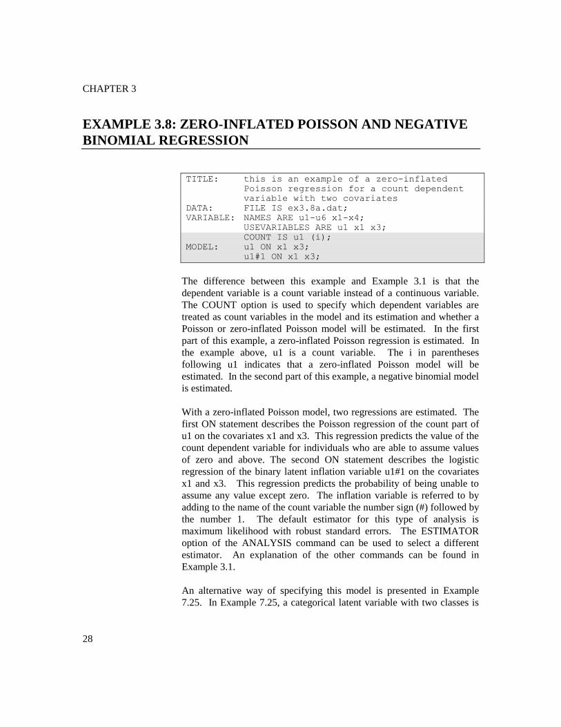
The difference between this example and Example 3.1 is that the
dependent variable is a count variable instead of a continuous variable.
The COUNT option is used to specify which dependent variables are
treated as count variables in the model and its estimation and whether a
Poisson or zero-inflated Poisson model will be estimated. In the first
part of this example, a zero-inflated Poisson regression is estimated. In
the example above, u1 is a count variable. The i in parentheses
following u1 indicates that a zero-inflated Poisson model will be
estimated. In the second part of this example, a negative binomial model
is estimated.
With a zero-inflated Poisson model, two regressions are estimated. The
first ON statement describes the Poisson regression of the count part of
u1 on the covariates x1 and x3. This regression predicts the value of the
count dependent variable for individuals who are able to assume values
of zero and above. The second ON statement describes the logistic
regression of the binary latent inflation variable u1#1 on the covariates
x1 and x3. This regression predicts the probability of being unable to
assume any value except zero. The inflation variable is referred to by
adding to the name of the count variable the number sign (#) followed by
the number 1. The default estimator for this type of analysis is
maximum likelihood with robust standard errors. The ESTIMATOR
option of the ANALYSIS command can be used to select a different
estimator. An explanation of the other commands can be found in
Example 3.1.
An alternative way of specifying this model is presented in Example
7.25. In Example 7.25, a categorical latent variable with two classes is

Examples: Regression And Path Analysis
29
used to represent individuals who are able to assume values of zero and
above and individuals who are unable to assume any value except zero.
This approach allows the estimation of the probability of being in each
class and the posterior probabilities of being in each class for each
individual.
TITLE: this is an example of a negative binomial
model for a count dependent variable with
two covariates
DATA: FILE IS ex3.8b.dat;
VARIABLE: NAMES ARE u1-u6 x1-x4;
USEVARIABLES ARE u1 x1 x3;
COUNT IS u1 (nb);
MODEL: u1 ON x1 x3;
The difference between this part of the example and the first part is that
a regression for a count outcome using a negative binomial model is
estimated instead of a zero-inflated Poisson model. The negative
binomial model estimates a dispersion parameter for each of the
outcomes (Long, 1997; Hilbe, 2011).
The COUNT option is used to specify which dependent variables are
treated as count variables in the model and its estimation and which type
of model is estimated. The nb in parentheses following u1 indicates that
a negative binomial model will be estimated. The dispersion parameter
can be referred to using the name of the count variable. An explanation
of the other commands can be found in the first part of this example and
in Example 3.1.
EXAMPLE 3.9: RANDOM COEFFICIENT REGRESSION
TITLE: this is an example of a random coefficient
regression
DATA: FILE IS ex3.9.dat;
VARIABLE: NAMES ARE y x1 x2;
DEFINE: CENTER x1 x2 (GRANDMEAN);
ANALYSIS: TYPE = RANDOM;
MODEL: s | y ON x1;
s WITH y;
y s ON x2;
CHAPTER 3
30
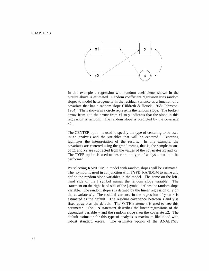
In this example a regression with random coefficients shown in the
picture above is estimated. Random coefficient regression uses random
slopes to model heterogeneity in the residual variance as a function of a
covariate that has a random slope (Hildreth & Houck, 1968; Johnston,
1984). The s shown in a circle represents the random slope. The broken
arrow from s to the arrow from x1 to y indicates that the slope in this
regression is random. The random slope is predicted by the covariate
x2.
The CENTER option is used to specify the type of centering to be used
in an analysis and the variables that will be centered. Centering
facilitates the interpretation of the results. In this example, the
covariates are centered using the grand means, that is, the sample means
of x1 and x2 are subtracted from the values of the covariates x1 and x2.
The TYPE option is used to describe the type of analysis that is to be
performed.
By selecting RANDOM, a model with random slopes will be estimated.
The | symbol is used in conjunction with TYPE=RANDOM to name and
define the random slope variables in the model. The name on the left-
hand side of the | symbol names the random slope variable. The
statement on the right-hand side of the | symbol defines the random slope
variable. The random slope s is defined by the linear regression of y on
the covariate x1. The residual variance in the regression of y on x is
estimated as the default. The residual covariance between s and y is
fixed at zero as the default. The WITH statement is used to free this
parameter. The ON statement describes the linear regressions of the
dependent variable y and the random slope s on the covariate x2. The
default estimator for this type of analysis is maximum likelihood with
robust standard errors. The estimator option of the ANALYSIS

Examples: Regression And Path Analysis
31
command can be used to select a different estimator. An explanation of
the other commands can be found in Example 3.1.
EXAMPLE 3.10: NON-LINEAR CONSTRAINT ON THE LOGIT
PARAMETERS OF AN UNORDERED CATEGORICAL
(NOMINAL) VARIABLE
TITLE: this is an example of non-linear
constraint on the logit parameters of an
unordered categorical (nominal) variable
DATA: FILE IS ex3.10.dat;
VARIABLE: NAMES ARE u;
NOMINAL = u;
MODEL: [u#1] (p1);
[u#2] (p2);
[u#3] (p2);
MODEL CONSTRAINT:
p2 = log ((exp (p1) – 1)/2 – 1);
In this example, theory specifies the following probabilities for the four
categories of an unordered categorical (nominal) variable: ½ + ¼ p, ¼
(1-p), ¼ (1-p), ¼ p, where p is a probability parameter to be estimated.
These restrictions on the category probabilities correspond to non-linear
constraints on the logit parameters for the categories in the multinomial
logistic model. This example is based on Dempster, Laird, and Rubin
(1977, p. 2).
The NOMINAL option is used to specify which dependent variables are
treated as unordered categorical (nominal) variables in the model and its
estimation. In the example above, u is a four-category unordered
variable. The program determines the number of categories. The
categories of an unordered categorical variable are referred to by adding
to the name of the unordered categorical variable the number sign (#)
followed by the number of the category. In this example, u#1 refers to
the first category of u, u#2 refers to the second category of u, and u#3
refers to the third category of u.
In the MODEL command, parameters are given labels by placing a name
in parentheses after the parameter. The logit parameter for category one
is referred to as p1; the logit parameter for category two is referred to as
p2; and the logit parameter for category three is also referred to as p2.

CHAPTER 3
32
When two parameters are referred to using the same label, they are held
equal. The MODEL CONSTRAINT command is used to define linear
and non-linear constraints on the parameters in the model. The non-
linear constraint for the logits follows from the four probabilities given
above after some algebra. The default estimator for this type of analysis
is maximum likelihood with robust standard errors. The ESTIMATOR
option of the ANALYSIS command can be used to select a different
estimator. An explanation of the other commands can be found in
Example 3.1.
EXAMPLE 3.11: PATH ANALYSIS WITH CONTINUOUS
DEPENDENT VARIABLES
TITLE: this is an example of a path analysis
with continuous dependent variables
DATA: FILE IS ex3.11.dat;
VARIABLE: NAMES ARE y1-y6 x1-x4;
USEVARIABLES ARE y1-y3 x1-x3;
MODEL: y1 y2 ON x1 x2 x3;
y3 ON y1 y2 x2;
In this example, the path analysis model shown in the picture above is
estimated. The dependent variables in the analysis are continuous. Two
of the dependent variables y1 and y2 mediate the effects of the
covariates x1, x2, and x3 on the dependent variable y3.

Examples: Regression And Path Analysis
33
The first ON statement describes the linear regressions of y1 and y2 on
the covariates x1, x2, and x3. The second ON statement describes the
linear regression of y3 on the mediating variables y1 and y2 and the
covariate x2. The residual variances of the three dependent variables are
estimated as the default. The residuals are not correlated as the default.
As in regression analysis, it is not necessary to refer to the means,
variances, and covariances among the x variables in the MODEL
command because the parameters of the x variables are not part of the
model estimation. Because the model does not impose restrictions on
the parameters of the x variables, these parameters can be estimated
separately as the sample values. The default estimator for this type of
analysis is maximum likelihood. The ESTIMATOR option of the
ANALYSIS command can be used to select a different estimator. An
explanation of the other commands can be found in Example 3.1.
EXAMPLE 3.12: PATH ANALYSIS WITH CATEGORICAL
DEPENDENT VARIABLES
TITLE: this is an example of a path analysis
with categorical dependent variables
DATA: FILE IS ex3.12.dat;
VARIABLE: NAMES ARE u1-u6 x1-x4;
USEVARIABLES ARE u1-u3 x1-x3;
CATEGORICAL ARE u1-u3;
MODEL: u1 u2 ON x1 x2 x3;
u3 ON u1 u2 x2;
The difference between this example and Example 3.11 is that the
dependent variables are binary and/or ordered categorical (ordinal)
variables instead of continuous variables. The CATEGORICAL option
is used to specify which dependent variables are treated as binary or
ordered categorical (ordinal) variables in the model and its estimation.
In the example above, u1, u2, and u3 are binary or ordered categorical
variables. The program determines the number of categories for each
variable. The first ON statement describes the probit regressions of u1
and u2 on the covariates x1, x2, and x3. The second ON statement
describes the probit regression of u3 on the mediating variables u1 and
u2 and the covariate x2. The default estimator for this type of analysis is
a robust weighted least squares estimator. The ESTIMATOR option of
the ANALYSIS command can be used to select a different estimator. If
the maximum likelihood estimator is selected, the regressions are

CHAPTER 3
34
logistic regressions. An explanation of the other commands can be
found in Example 3.1.
EXAMPLE 3.13: PATH ANALYSIS WITH CATEGORICAL
DEPENDENT VARIABLES USING THE THETA
PARAMETERIZATION
TITLE: this is an example of a path analysis
with categorical dependent variables using
the Theta parameterization
DATA: FILE IS ex3.13.dat;
VARIABLE: NAMES ARE u1-u6 x1-x4;
USEVARIABLES ARE u1-u3 x1-x3;
CATEGORICAL ARE u1-u3;
ANALYSIS: PARAMETERIZATION = THETA;
MODEL: u1 u2 ON x1 x2 x3;
u3 ON u1 u2 x2;
The difference between this example and Example 3.12 is that the Theta
parameterization is used instead of the default Delta parameterization.
In the Delta parameterization, scale factors for continuous latent
response variables of observed categorical dependent variables are
allowed to be parameters in the model, but residual variances for
continuous latent response variables are not. In the Theta
parameterization, residual variances for continuous latent response
variables of observed categorical dependent variables are allowed to be
parameters in the model, but scale factors for continuous latent response
variables are not. An explanation of the other commands can be found
in Examples 3.1 and 3.12.

Examples: Regression And Path Analysis
35
EXAMPLE 3.14: PATH ANALYSIS WITH A COMBINATION
OF CONTINUOUS AND CATEGORICAL DEPENDENT
VARIABLES
TITLE: this is an example of a path analysis
with a combination of continuous and
categorical dependent variables
DATA: FILE IS ex3.14.dat;
VARIABLE: NAMES ARE y1 y2 u1 y4-y6 x1-x4;
USEVARIABLES ARE y1-u1 x1-x3;
CATEGORICAL IS u1;
MODEL: y1 y2 ON x1 x2 x3;
u1 ON y1 y2 x2;
The difference between this example and Example 3.11 is that the
dependent variables are a combination of continuous and binary or
ordered categorical (ordinal) variables instead of all continuous
variables. The CATEGORICAL option is used to specify which
dependent variables are treated as binary or ordered categorical (ordinal)
variables in the model and its estimation. In the example above, y1 and
y2 are continuous variables and u1 is a binary or ordered categorical
variable. The program determines the number of categories. The first
ON statement describes the linear regressions of y1 and y2 on the
covariates x1, x2, and x3. The second ON statement describes the probit
regression of u1 on the mediating variables y1 and y2 and the covariate
x2. The default estimator for this type of analysis is a robust weighted
least squares estimator. The ESTIMATOR option of the ANALYSIS
command can be used to select a different estimator. If a maximum
likelihood estimator is selected, the regression for u1 is a logistic
regression. An explanation of the other commands can be found in
Example 3.1.
CHAPTER 3
36
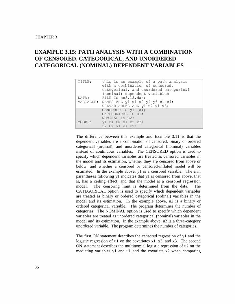
EXAMPLE 3.15: PATH ANALYSIS WITH A COMBINATION
OF CENSORED, CATEGORICAL, AND UNORDERED
CATEGORICAL (NOMINAL) DEPENDENT VARIABLES
TITLE: this is an example of a path analysis
with a combination of censored,
categorical, and unordered categorical
(nominal) dependent variables
DATA: FILE IS ex3.15.dat;
VARIABLE: NAMES ARE y1 u1 u2 y4-y6 x1-x4;
USEVARIABLES ARE y1-u2 x1-x3;
CENSORED IS y1 (a);
CATEGORICAL IS u1;
NOMINAL IS u2;
MODEL: y1 u1 ON x1 x2 x3;
u2 ON y1 u1 x2;
The difference between this example and Example 3.11 is that the
dependent variables are a combination of censored, binary or ordered
categorical (ordinal), and unordered categorical (nominal) variables
instead of continuous variables. The CENSORED option is used to
specify which dependent variables are treated as censored variables in
the model and its estimation, whether they are censored from above or
below, and whether a censored or censored-inflated model will be
estimated. In the example above, y1 is a censored variable. The a in
parentheses following y1 indicates that y1 is censored from above, that
is, has a ceiling effect, and that the model is a censored regression
model. The censoring limit is determined from the data. The
CATEGORICAL option is used to specify which dependent variables
are treated as binary or ordered categorical (ordinal) variables in the
model and its estimation. In the example above, u1 is a binary or
ordered categorical variable. The program determines the number of
categories. The NOMINAL option is used to specify which dependent
variables are treated as unordered categorical (nominal) variables in the
model and its estimation. In the example above, u2 is a three-category
unordered variable. The program determines the number of categories.
The first ON statement describes the censored regression of y1 and the
logistic regression of u1 on the covariates x1, x2, and x3. The second
ON statement describes the multinomial logistic regression of u2 on the
mediating variables y1 and u1 and the covariate x2 when comparing

Examples: Regression And Path Analysis
37
categories one and two of u2 to the third category of u2. The intercept
and slopes of the last category are fixed at zero as the default. The
default estimator for this type of analysis is maximum likelihood with
robust standard errors. The ESTIMATOR option of the ANALYSIS
command can be used to select a different estimator. An explanation of
the other commands can be found in Example 3.1.
Following is an alternative specification of the multinomial logistic
regression of u2 on the mediating variables y1 and u1 and the covariate
x2:
u2#1 u2#2 ON y1 u1 x2;
where u2#1 refers to the first category of u2 and u2#2 refers to the
second category of u2. The categories of an unordered categorical
variable are referred to by adding to the name of the unordered
categorical variable the number sign (#) followed by the number of the
category. This alternative specification allows individual parameters to
be referred to in the MODEL command for the purpose of giving starting
values or placing restrictions.
EXAMPLE 3.16: PATH ANALYSIS WITH CONTINUOUS
DEPENDENT VARIABLES, BOOTSTRAPPED STANDARD
ERRORS, INDIRECT EFFECTS, AND NON-SYMMETRIC
BOOTSTRAP CONFIDENCE INTERVALS
TITLE: this is an example of a path analysis
with continuous dependent variables,
bootstrapped standard errors, indirect
effects, and non-symmetric bootstrap
confidence intervals
DATA: FILE IS ex3.16.dat;
VARIABLE: NAMES ARE y1-y6 x1-x4;
USEVARIABLES ARE y1-y3 x1-x3;
ANALYSIS: BOOTSTRAP = 1000;
MODEL: y1 y2 ON x1 x2 x3;
y3 ON y1 y2 x2;
MODEL INDIRECT:
y3 IND y1 x1;
y3 IND y2 x1;
OUTPUT: CINTERVAL (BOOTSTRAP);

CHAPTER 3
38
The difference between this example and Example 3.11 is that
bootstrapped standard errors, indirect effects, and non-symmetric
bootstrap confidence intervals are requested. The BOOTSTRAP option
is used to request bootstrapping and to specify the number of bootstrap
draws to be used in the computation. When the BOOTSTRAP option is
used alone, bootstrap standard errors of the model parameter estimates
are obtained. When the BOOTSTRAP option is used in conjunction
with the CINTERVAL(BOOTSTRAP) option of the OUTPUT
command, bootstrap standard errors of the model parameter estimates
and non-symmetric bootstrap confidence intervals for the model
parameter estimates are obtained. The BOOTSTRAP option can be used
in conjunction with the MODEL INDIRECT command to obtain
bootstrap standard errors for indirect effects. When both MODEL
INDIRECT and CINTERVAL(BOOTSTRAP) are used, bootstrapped
standard errors and bootstrap confidence intervals are obtained for the
indirect effects. By selecting BOOTSTRAP=1000, bootstrapped
standard errors will be computed using 1000 draws.
The MODEL INDIRECT command is used to request indirect effects
and their standard errors. Total indirect, specific indirect, and total
effects are obtained using the IND and VIA options of the MODEL
INDIRECT command. The IND option is used to request a specific
indirect effect or a set of indirect effects. In the IND statements above,
the variable on the left-hand side of IND is the dependent variable. The
last variable on the right-hand side of IND is the independent variable.
Other variables on the right-hand side of IND are mediating variables.
The first IND statement requests the specific indirect effect from x1 to
y1 to y3. The second IND statement requests the specific indirect effect
from x1 to y2 to y3. Total effects are computed for all IND statements
that start and end with the same variables. An explanation of the other
commands can be found in Examples 3.1 and 3.11.
Examples: Regression And Path Analysis
39
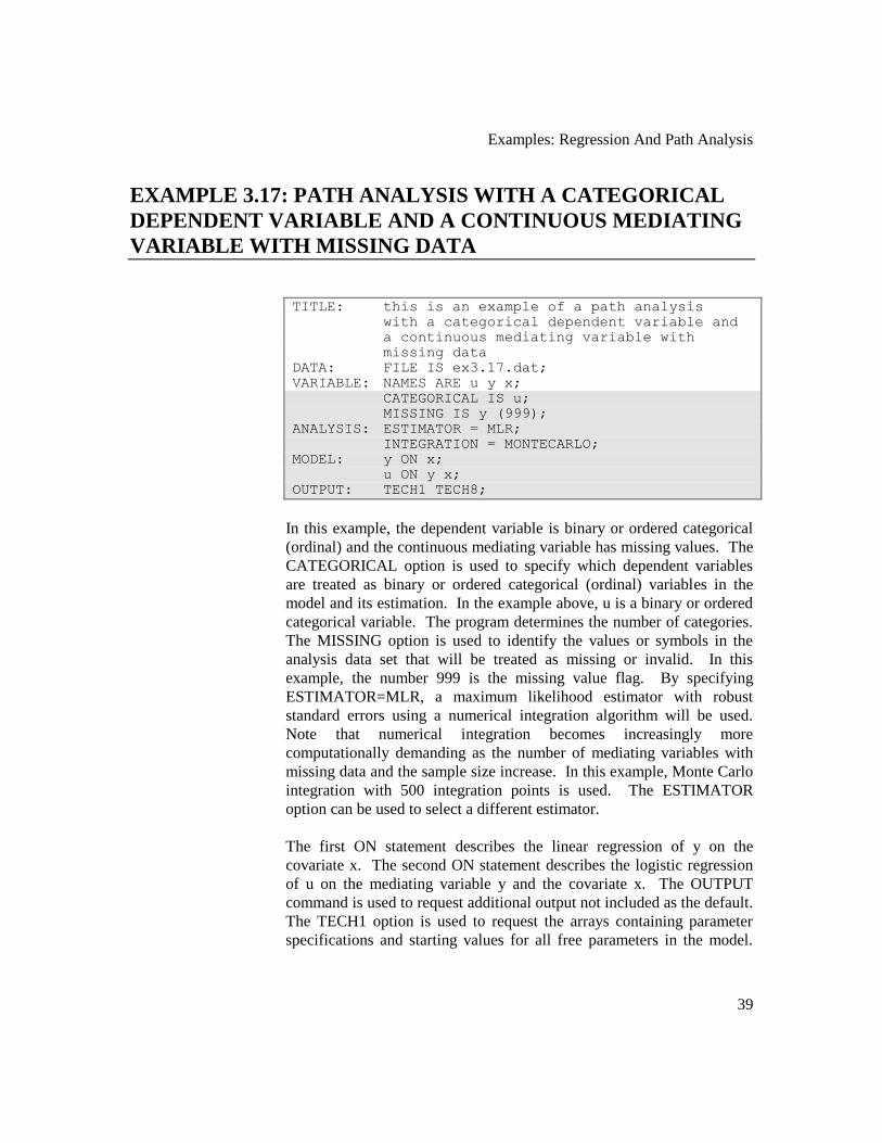
EXAMPLE 3.17: PATH ANALYSIS WITH A CATEGORICAL
DEPENDENT VARIABLE AND A CONTINUOUS MEDIATING
VARIABLE WITH MISSING DATA
TITLE: this is an example of a path analysis
with a categorical dependent variable and
a continuous mediating variable with
missing data
DATA: FILE IS ex3.17.dat;
VARIABLE: NAMES ARE u y x;
CATEGORICAL IS u;
MISSING IS y (999);
ANALYSIS: ESTIMATOR = MLR;
INTEGRATION = MONTECARLO;
MODEL: y ON x;
u ON y x;
OUTPUT: TECH1 TECH8;
In this example, the dependent variable is binary or ordered categorical
(ordinal) and the continuous mediating variable has missing values. The
CATEGORICAL option is used to specify which dependent variables
are treated as binary or ordered categorical (ordinal) variables in the
model and its estimation. In the example above, u is a binary or ordered
categorical variable. The program determines the number of categories.
The MISSING option is used to identify the values or symbols in the
analysis data set that will be treated as missing or invalid. In this
example, the number 999 is the missing value flag. By specifying
ESTIMATOR=MLR, a maximum likelihood estimator with robust
standard errors using a numerical integration algorithm will be used.
Note that numerical integration becomes increasingly more
computationally demanding as the number of mediating variables with
missing data and the sample size increase. In this example, Monte Carlo
integration with 500 integration points is used. The ESTIMATOR
option can be used to select a different estimator.
The first ON statement describes the linear regression of y on the
covariate x. The second ON statement describes the logistic regression
of u on the mediating variable y and the covariate x. The OUTPUT
command is used to request additional output not included as the default.
The TECH1 option is used to request the arrays containing parameter
specifications and starting values for all free parameters in the model.

CHAPTER 3
40
The TECH8 option is used to request that the optimization history in
estimating the model be printed in the output. TECH8 is printed to the
screen during the computations as the default. TECH8 screen printing is
useful for determining how long the analysis takes. An explanation of
the other commands can be found in Example 3.1.
EXAMPLE 3.18: MODERATED MEDIATION WITH A PLOT
OF THE INDIRECT EFFECT
TITLE: this is an example of moderated mediation
with a plot of the indirect effect
DATA: FILE = ex3.18.dat;
VARIABLE: NAMES = y m x z;
USEVARIABLES = y m x z xz;
DEFINE: xz = x*z;
ANALYSIS: ESTIMATOR = BAYES;
PROCESSORS = 2;
BITERATIONS = (30000);
MODEL: y ON m (b)
x z;
m ON x (gamma1)
z
xz (gamma2);
MODEL CONSTRAINT:
PLOT(indirect);
LOOP(mod,-2,2,0.1);
indirect = b*(gamma1+gamma2*mod);
PLOT: TYPE = PLOT2;
OUTPUT: TECH8;
In this example, a moderated mediation analysis with a plot of the
indirect effect is carried out (Preacher, Rucker, & Hayes, 2007). The
variable z moderates the relationship between the mediator m and the
covariate x. The DEFINE command is used to create the variable xz
which is the interaction between the moderator z and the covariate x.
The variable xz must be included on the USEVARIABLES list after the
original variables in order to be used in the analysis.
By specifying ESTIMATOR=BAYES, a Bayesian analysis will be
carried out. In Bayesian estimation, the default is to use two
independent Markov chain Monte Carlo (MCMC) chains. If multiple
processors are available, using PROCESSORS=2 will speed up
computations. The BITERATIONS option is used to specify the
Examples: Regression And Path Analysis
41
maximum and minimum number of iterations for each Markov chain
Monte Carlo (MCMC) chain when the potential scale reduction (PSR)
convergence criterion (Gelman & Rubin, 1992) is used. Using a number
in parentheses, the BITERATIONS option specifies that a minimum of
30,000 and a maximum of the default of 50,000 iterations will be used.
The large minimum value is chosen to obtain a smooth plot.
In the MODEL command, the first ON statement describes the linear
regression of y on the mediator m, the covariate x, and the moderator z.
The second ON statement describes the linear regression of the mediator
m on the covariate x, the moderator z, and the interaction xz. The
intercepts and residual variances of y and m are estimated and the
residuals are not correlated as the default.
In MODEL CONSTRAINT, the LOOP option is used in conjunction
with the PLOT option to create plots of variables. In this example, the
indirect effect defined in MODEL CONSTRAINT will be plotted. The
PLOT option names the variable that will be plotted on the y-axis. The
LOOP option names the variable that will be plotted on the x-axis, gives
the numbers that are the lower and upper values of the variable, and the
incremental value of the variable to be used in the computations. In this
example, the variable indirect will be on the y-axis and the variable mod
will be on the x-axis. The variable mod, as in moderation, varies over
the range of z that is of interest such as two standard deviations away
from its mean. Corresponding to the case of z being standardized, the
lower and upper values of mod are -2 and 2 and 0.1 is the incremental
value of mod to use in the computations. When mod appears in a
MODEL CONSTRAINT statement involving a new parameter, that
statement is evaluated for each value of mod specified by the LOOP
option. For example, the first value of mod is -2; the second value of
mod is -2 plus 0.1 or -1.9; the third value of mod is -1.9 plus 0.1 or -1.8;
the last value of mod is 2.
Using TYPE=PLOT2 in the PLOT command, the plot of indirect and
mod can be viewed by choosing Loop plots from the Plot menu of the
Mplus Editor. The plot presents the computed values along with a 95%
confidence interval. For Bayesian estimation, the default is credibility
intervals of the posterior distribution with equal tail percentages. The
CINTERVAL option of the OUTPUT command can be used to obtain
credibility intervals of the posterior distribution that give the highest

CHAPTER 3
42
posterior density. An explanation of the other commands can be found
in Example 3.1.
Related Documents