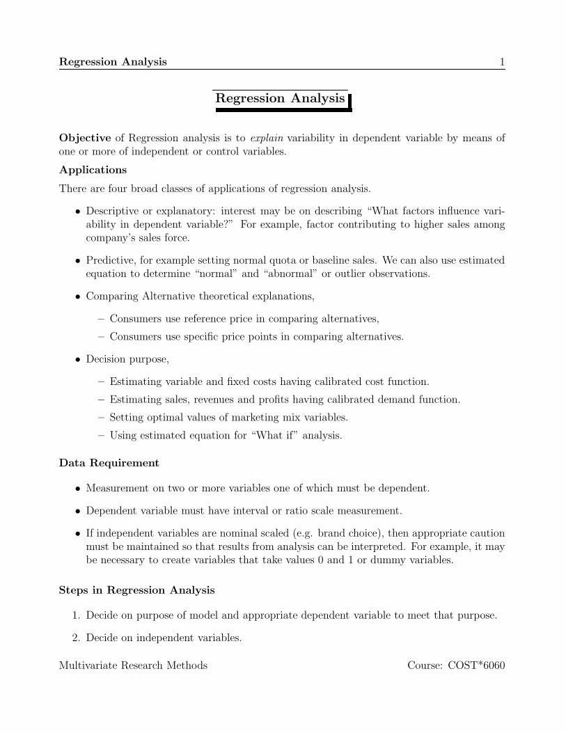
Regression Analysis 1 Regression Analysis Objective of Regression analysis is to explain variability in dependent variable by means of one or more of independent or control variables. Applications There are four broad classes of applications of regression analysis. • Descriptive or explanatory: interest may be on describing “What factors influence vari- ability in dependent variable?” For example, factor contributing to higher sales among company’s sales force. • Predictive, for example setting normal quota or baseline sales. We can also use estimated equation to determine “normal” and “abnormal” or outlier observations. • Comparing Alternative theoretical explanations, – Consumers use reference price in comparing alternatives, – Consumers use specific price points in comparing alternatives. • Decision purpose, – Estimating variable and fixed costs having calibrated cost function. – Estimating sales, revenues and profits having calibrated demand function. – Setting optimal values of marketing mix variables. – Using estimated equation for “What if” analysis. Data Requirement • Measurement on two or more variables one of which must be dependent. • Dependent variable must have interval or ratio scale measurement. • If independent variables are nominal scaled (e.g. brand choice), then appropriate caution must be maintained so that results from analysis can be interpreted. For example, it may be necessary to create variables that take values 0 and 1 or dummy variables. Steps in Regression Analysis 1. Decide on purpose of model and appropriate dependent variable to meet that purpose. 2. Decide on independent variables. Multivariate Research Methods Course: COST*6060

Welcome message from author
This document is posted to help you gain knowledge. Please leave a comment to let me know what you think about it! Share it to your friends and learn new things together.
Transcript
Regression Analysis 1
Regression Analysis
Objective of Regression analysis is to explain variability in dependent variable by means ofone or more of independent or control variables.
Applications
There are four broad classes of applications of regression analysis.
• Descriptive or explanatory: interest may be on describing “What factors influence vari-ability in dependent variable?” For example, factor contributing to higher sales amongcompany’s sales force.
• Predictive, for example setting normal quota or baseline sales. We can also use estimatedequation to determine “normal” and “abnormal” or outlier observations.
• Comparing Alternative theoretical explanations,
– Consumers use reference price in comparing alternatives,
– Consumers use specific price points in comparing alternatives.
• Decision purpose,
– Estimating variable and fixed costs having calibrated cost function.
– Estimating sales, revenues and profits having calibrated demand function.
– Setting optimal values of marketing mix variables.
– Using estimated equation for “What if” analysis.
Data Requirement
• Measurement on two or more variables one of which must be dependent.
• Dependent variable must have interval or ratio scale measurement.
• If independent variables are nominal scaled (e.g. brand choice), then appropriate cautionmust be maintained so that results from analysis can be interpreted. For example, it maybe necessary to create variables that take values 0 and 1 or dummy variables.
Steps in Regression Analysis
1. Decide on purpose of model and appropriate dependent variable to meet that purpose.
2. Decide on independent variables.
Multivariate Research Methods Course: COST*6060
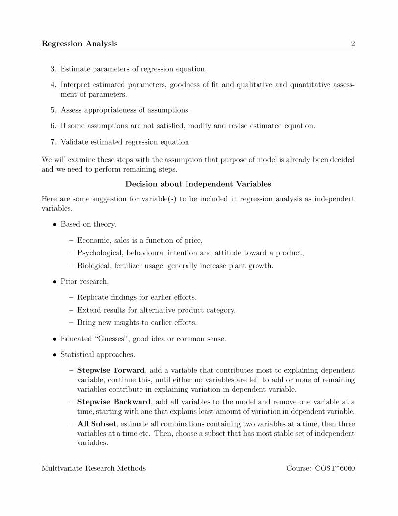
Regression Analysis 2
3. Estimate parameters of regression equation.
4. Interpret estimated parameters, goodness of fit and qualitative and quantitative assess-ment of parameters.
5. Assess appropriateness of assumptions.
6. If some assumptions are not satisfied, modify and revise estimated equation.
7. Validate estimated regression equation.
We will examine these steps with the assumption that purpose of model is already been decidedand we need to perform remaining steps.
Decision about Independent Variables
Here are some suggestion for variable(s) to be included in regression analysis as independentvariables.
• Based on theory.
– Economic, sales is a function of price,
– Psychological, behavioural intention and attitude toward a product,
– Biological, fertilizer usage, generally increase plant growth.
• Prior research,
– Replicate findings for earlier efforts.
– Extend results for alternative product category.
– Bring new insights to earlier efforts.
• Educated “Guesses”, good idea or common sense.
• Statistical approaches.
– Stepwise Forward, add a variable that contributes most to explaining dependentvariable, continue this, until either no variables are left to add or none of remainingvariables contribute in explaining variation in dependent variable.
– Stepwise Backward, add all variables to the model and remove one variable at atime, starting with one that explains least amount of variation in dependent variable.
– All Subset, estimate all combinations containing two variables at a time, then threevariables at a time etc. Then, choose a subset that has most stable set of independentvariables.
Multivariate Research Methods Course: COST*6060
Regression Analysis 3
• All variables contained in dataset.
Estimating Parameters
• Method of least squares, or
• Method of maximum likelihood, or
• Weighted least squares, or
• Method of least absolute deviations.
We will examine several alternative approaches to estimate parameters including situationwhere we have only two observations.
A Simple Regression Model can be written as
Value of Dependent variable = Constant +
Slope × Value of Indep. variable + Error
y = a + b × x + E
• Constant (a), Slope (b) and Error (E) are unknown.
• You observe N pair of values of dependent and independent variables.
• Regression analysis provides reasonable (statistically unbiased) values for slope(s) andintercept.
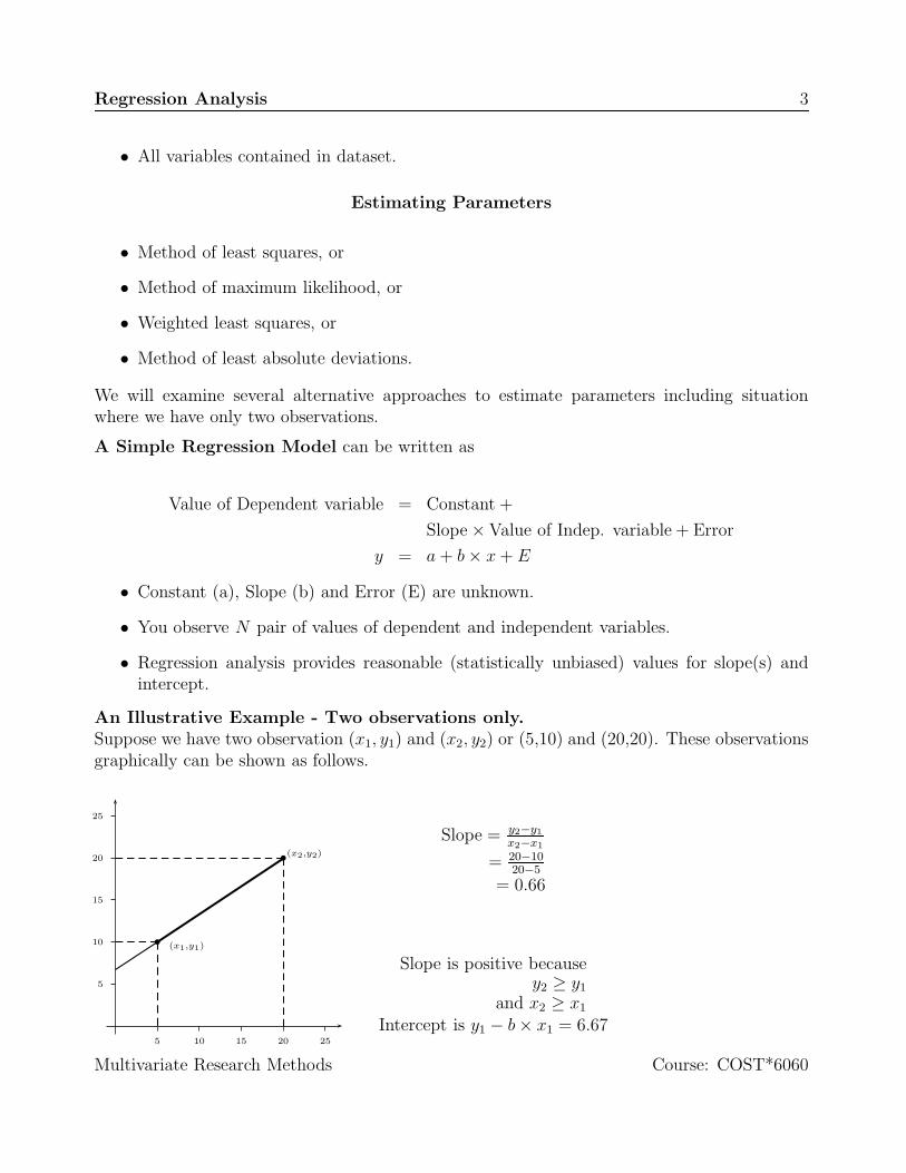
An Illustrative Example - Two observations only.Suppose we have two observation (x1, y1) and (x2, y2) or (5,10) and (20,20). These observationsgraphically can be shown as follows.
5 10 15 20 25
5
10
15
20
25
(x1,y1)
(x2,y2)
Slope = y2−y1
x2−x1
= 20−1020−5
= 0.66
Slope is positive becausey2 ≥ y1
and x2 ≥ x1
Intercept is y1 − b × x1 = 6.67
Multivariate Research Methods Course: COST*6060
Regression Analysis 4
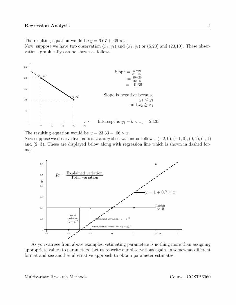
The resulting equation would be y = 6.67 + .66 × x.Now, suppose we have two observation (x1, y1) and (x2, y2) or (5,20) and (20,10). These obser-vations graphically can be shown as follows.
5 10 15 20 25
5
10
15
20
25
(x1,y1)
(x2,y2)
Slope = y2−y1
x2−x1
= 10−2020−5
= −0.66
Slope is negative becausey2 < y1
and x2 ≥ x1
Intercept is y1 − b × x1 = 23.33
The resulting equation would be y = 23.33 − .66 × x.Now suppose we observe five pairs of x and y observations as follows: (−2, 0), (−1, 0), (0, 1), (1, 1)and (2, 3). These are displayed below along with regression line which is shown in dashed for-mat.
−3 −2 −1 0 1 2 3
0
0.5
1.0
1.5
2.0
2.5
3.0
x
y
meanor y
y = 1 + 0.7 × x
Totalvariation
(y − y)2
Unexplained variation (y − y)2
Explained variation (y − y)2
R2 = Explained variationTotal variation
As you can see from above examples, estimating parameters is nothing more than assigningappropriate values to parameters. Let us re-write our observations again, in somewhat differentformat and see another alternative approach to obtain parameter estimates.
Multivariate Research Methods Course: COST*6060
Regression Analysis 5
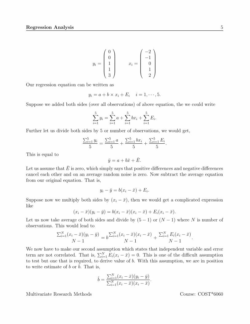
yi =
00113
xi =
−2−1
012
Our regression equation can be written as
yi = a + b × xi + Ei i = 1, · · · , 5.
Suppose we added both sides (over all observations) of above equation, the we could write
5∑
i=1
yi =5∑
i=1
a +5∑
i=1
bxi +5∑
i=1
Ei.
Further let us divide both sides by 5 or number of observations, we would get,∑5
i=1 yi
5=
∑5i=1 a
5+
∑5i=1 bxi
5+
∑5i=1 Ei
5.
This is equal toy = a + bx + E.
Let us assume that E is zero, which simply says that positive differences and negative differencescancel each other and on an average random noise is zero. Now subtract the average equationfrom our original equation. That is,
yi − y = b(xi − x) + Ei.
Suppose now we multiply both sides by (xi − x), then we would get a complicated expressionlike
(xi − x)(yi − y) = b(xi − x)(xi − x) + Ei(xi − x).
Let us now take average of both sides and divide by (5 − 1) or (N − 1) where N is number ofobservations. This would lead to
∑Ni=1(xi − x)(yi − y)
N − 1= b
∑Ni=1(xi − x)(xi − x)
N − 1+
∑Ni=1 Ei(xi − x)
N − 1.
We now have to make our second assumption which states that independent variable and errorterm are not correlated. That is,
∑Ni=1 Ei(xi − x) = 0. This is one of the difficult assumption
to test but one that is required, to derive value of b. With this assumption, we are in positionto write estimate of b or b. That is,
b =
∑Ni=1(xi − x)(yi − y)
∑Ni=1(xi − x)(xi − x)
.
Multivariate Research Methods Course: COST*6060
Regression Analysis 6
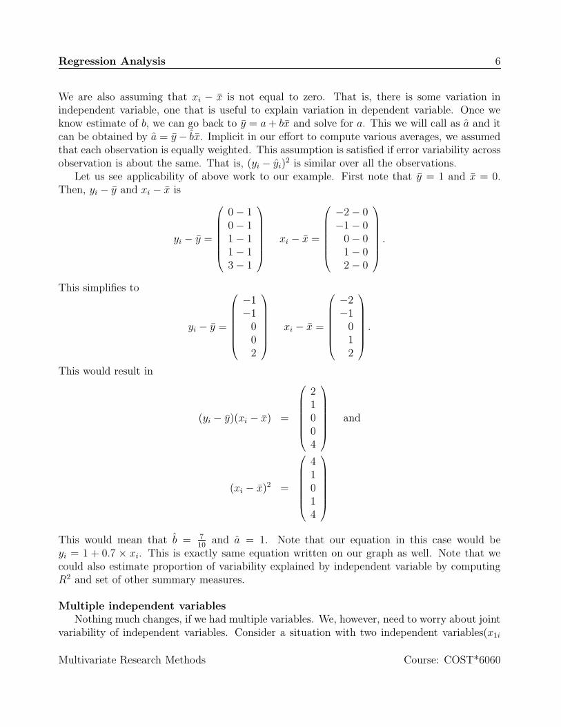
We are also assuming that xi − x is not equal to zero. That is, there is some variation inindependent variable, one that is useful to explain variation in dependent variable. Once weknow estimate of b, we can go back to y = a + bx and solve for a. This we will call as a and itcan be obtained by a = y − bx. Implicit in our effort to compute various averages, we assumedthat each observation is equally weighted. This assumption is satisfied if error variability acrossobservation is about the same. That is, (yi − yi)
2 is similar over all the observations.Let us see applicability of above work to our example. First note that y = 1 and x = 0.
Then, yi − y and xi − x is
yi − y =
0 − 10 − 11 − 11 − 13 − 1
xi − x =
−2 − 0−1 − 0
0 − 01 − 02 − 0
.
This simplifies to
yi − y =
−1−1
002
xi − x =
−2−1
012
.
This would result in
(yi − y)(xi − x) =
21004
and
(xi − x)2 =
41014
This would mean that b = 710
and a = 1. Note that our equation in this case would beyi = 1 + 0.7 × xi. This is exactly same equation written on our graph as well. Note that wecould also estimate proportion of variability explained by independent variable by computingR2 and set of other summary measures.
Multiple independent variablesNothing much changes, if we had multiple variables. We, however, need to worry about joint
variability of independent variables. Consider a situation with two independent variables(x1i
Multivariate Research Methods Course: COST*6060
Regression Analysis 7
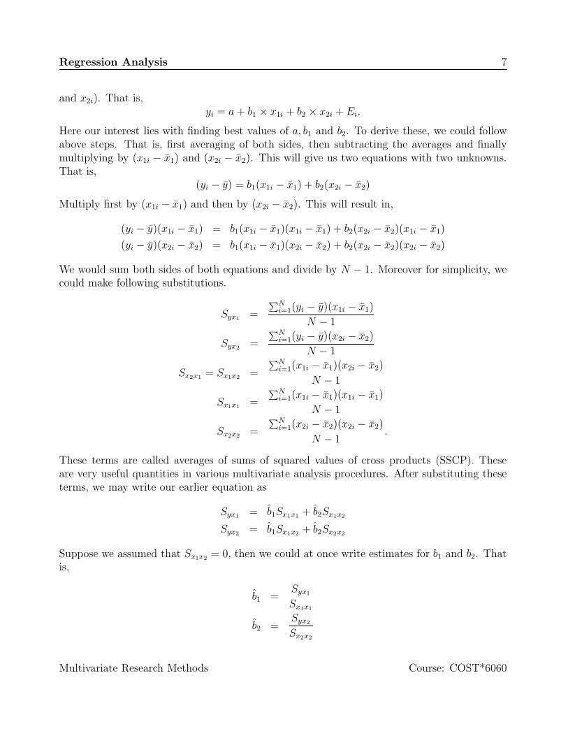
and x2i). That is,yi = a + b1 × x1i + b2 × x2i + Ei.
Here our interest lies with finding best values of a, b1 and b2. To derive these, we could followabove steps. That is, first averaging of both sides, then subtracting the averages and finallymultiplying by (x1i − x1) and (x2i − x2). This will give us two equations with two unknowns.That is,
(yi − y) = b1(x1i − x1) + b2(x2i − x2)
Multiply first by (x1i − x1) and then by (x2i − x2). This will result in,
(yi − y)(x1i − x1) = b1(x1i − x1)(x1i − x1) + b2(x2i − x2)(x1i − x1)
(yi − y)(x2i − x2) = b1(x1i − x1)(x2i − x2) + b2(x2i − x2)(x2i − x2)
We would sum both sides of both equations and divide by N − 1. Moreover for simplicity, wecould make following substitutions.
Syx1 =
∑Ni=1(yi − y)(x1i − x1)
N − 1
Syx2 =
∑Ni=1(yi − y)(x2i − x2)
N − 1
Sx2x1 = Sx1x2 =
∑Ni=1(x1i − x1)(x2i − x2)
N − 1
Sx1x1 =
∑Ni=1(x1i − x1)(x1i − x1)
N − 1
Sx2x2 =
∑Ni=1(x2i − x2)(x2i − x2)
N − 1.
These terms are called averages of sums of squared values of cross products (SSCP). Theseare very useful quantities in various multivariate analysis procedures. After substituting theseterms, we may write our earlier equation as
Syx1 = b1Sx1x1 + b2Sx1x2
Syx2 = b1Sx1x2 + b2Sx2x2
Suppose we assumed that Sx1x2 = 0, then we could at once write estimates for b1 and b2. Thatis,
b1 =Syx1
Sx1x1
b2 =Syx2
Sx2x2
Multivariate Research Methods Course: COST*6060
Regression Analysis 8
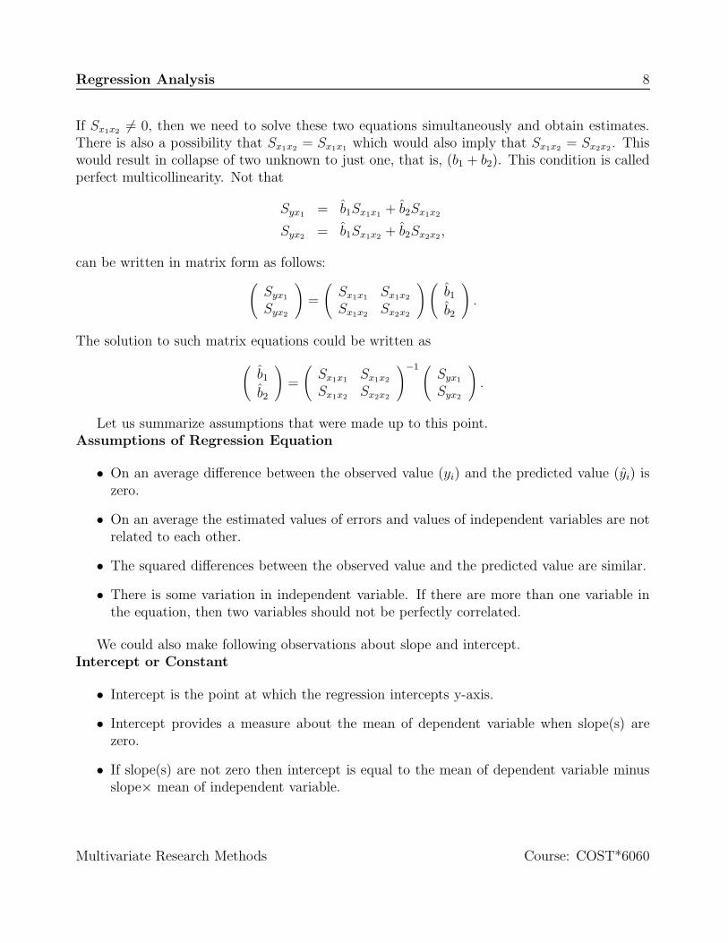
If Sx1x2 6= 0, then we need to solve these two equations simultaneously and obtain estimates.There is also a possibility that Sx1x2 = Sx1x1 which would also imply that Sx1x2 = Sx2x2. Thiswould result in collapse of two unknown to just one, that is, (b1 + b2). This condition is calledperfect multicollinearity. Not that
Syx1 = b1Sx1x1 + b2Sx1x2
Syx2 = b1Sx1x2 + b2Sx2x2 ,
can be written in matrix form as follows:(
Syx1
Syx2
)=
(Sx1x1 Sx1x2
Sx1x2 Sx2x2
)(b1
b2
).
The solution to such matrix equations could be written as
(b1
b2
)=
(Sx1x1 Sx1x2
Sx1x2 Sx2x2
)−1 (Syx1
Syx2
).
Let us summarize assumptions that were made up to this point.Assumptions of Regression Equation
• On an average difference between the observed value (yi) and the predicted value (yi) iszero.
• On an average the estimated values of errors and values of independent variables are notrelated to each other.
• The squared differences between the observed value and the predicted value are similar.
• There is some variation in independent variable. If there are more than one variable inthe equation, then two variables should not be perfectly correlated.
We could also make following observations about slope and intercept.Intercept or Constant
• Intercept is the point at which the regression intercepts y-axis.
• Intercept provides a measure about the mean of dependent variable when slope(s) arezero.
• If slope(s) are not zero then intercept is equal to the mean of dependent variable minusslope× mean of independent variable.
Multivariate Research Methods Course: COST*6060
Regression Analysis 9
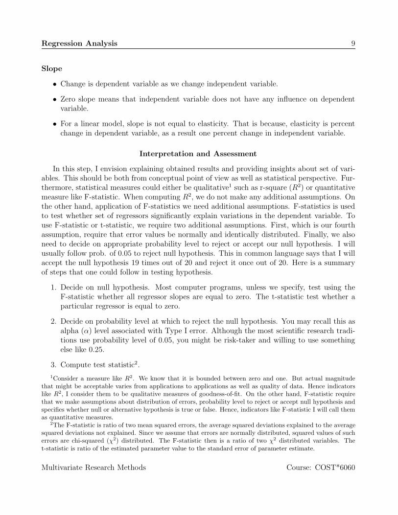
Slope
• Change is dependent variable as we change independent variable.
• Zero slope means that independent variable does not have any influence on dependentvariable.
• For a linear model, slope is not equal to elasticity. That is because, elasticity is percentchange in dependent variable, as a result one percent change in independent variable.
Interpretation and Assessment
In this step, I envision explaining obtained results and providing insights about set of vari-ables. This should be both from conceptual point of view as well as statistical perspective. Fur-thermore, statistical measures could either be qualitative1 such as r-square (R2) or quantitativemeasure like F-statistic. When computing R2, we do not make any additional assumptions. Onthe other hand, application of F-statistics we need additional assumptions. F-statistics is usedto test whether set of regressors significantly explain variations in the dependent variable. Touse F-statistic or t-statistic, we require two additional assumptions. First, which is our fourthassumption, require that error values be normally and identically distributed. Finally, we alsoneed to decide on appropriate probability level to reject or accept our null hypothesis. I willusually follow prob. of 0.05 to reject null hypothesis. This in common language says that I willaccept the null hypothesis 19 times out of 20 and reject it once out of 20. Here is a summaryof steps that one could follow in testing hypothesis.
1. Decide on null hypothesis. Most computer programs, unless we specify, test using theF-statistic whether all regressor slopes are equal to zero. The t-statistic test whether aparticular regressor is equal to zero.
2. Decide on probability level at which to reject the null hypothesis. You may recall this asalpha (α) level associated with Type I error. Although the most scientific research tradi-tions use probability level of 0.05, you might be risk-taker and willing to use somethingelse like 0.25.
3. Compute test statistic2.
1Consider a measure like R2. We know that it is bounded between zero and one. But actual magnitudethat might be acceptable varies from applications to applications as well as quality of data. Hence indicatorslike R2, I consider them to be qualitative measures of goodness-of-fit. On the other hand, F-statistic requirethat we make assumptions about distribution of errors, probability level to reject or accept null hypothesis andspecifies whether null or alternative hypothesis is true or false. Hence, indicators like F-statistic I will call themas quantitative measures.
2The F-statistic is ratio of two mean squared errors, the average squared deviations explained to the averagesquared deviations not explained. Since we assume that errors are normally distributed, squared values of sucherrors are chi-squared (χ2) distributed. The F-statistic then is a ratio of two χ2 distributed variables. Thet-statistic is ratio of the estimated parameter value to the standard error of parameter estimate.
Multivariate Research Methods Course: COST*6060
Regression Analysis 10
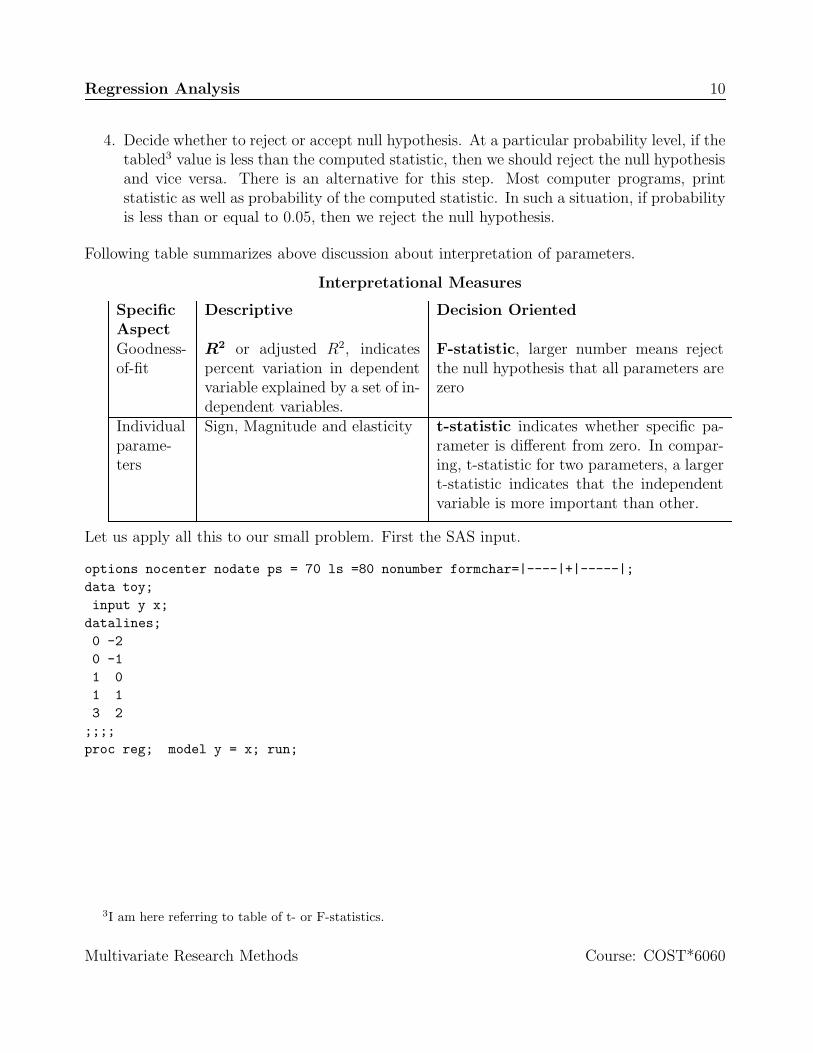
4. Decide whether to reject or accept null hypothesis. At a particular probability level, if thetabled3 value is less than the computed statistic, then we should reject the null hypothesisand vice versa. There is an alternative for this step. Most computer programs, printstatistic as well as probability of the computed statistic. In such a situation, if probabilityis less than or equal to 0.05, then we reject the null hypothesis.
Following table summarizes above discussion about interpretation of parameters.
Interpretational Measures
SpecificAspect
Descriptive Decision Oriented
Goodness-of-fit
R2 or adjusted R2, indicatespercent variation in dependentvariable explained by a set of in-dependent variables.
F-statistic, larger number means rejectthe null hypothesis that all parameters arezero
Individualparame-ters
Sign, Magnitude and elasticity t-statistic indicates whether specific pa-rameter is different from zero. In compar-ing, t-statistic for two parameters, a largert-statistic indicates that the independentvariable is more important than other.
Let us apply all this to our small problem. First the SAS input.
options nocenter nodate ps = 70 ls =80 nonumber formchar=|----|+|-----|;data toy;input y x;
datalines;0 -20 -11 01 13 2
;;;;proc reg; model y = x; run;
3I am here referring to table of t- or F-statistics.
Multivariate Research Methods Course: COST*6060
Regression Analysis 11
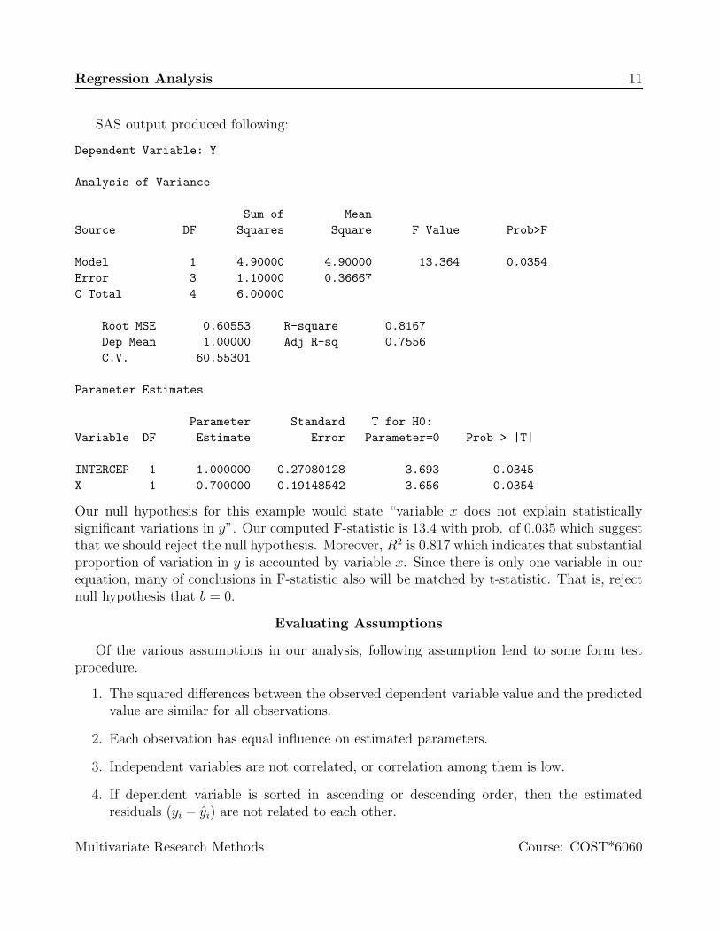
SAS output produced following:
Dependent Variable: Y
Analysis of Variance
Sum of MeanSource DF Squares Square F Value Prob>F
Model 1 4.90000 4.90000 13.364 0.0354Error 3 1.10000 0.36667C Total 4 6.00000
Root MSE 0.60553 R-square 0.8167Dep Mean 1.00000 Adj R-sq 0.7556C.V. 60.55301
Parameter Estimates
Parameter Standard T for H0:Variable DF Estimate Error Parameter=0 Prob > |T|
INTERCEP 1 1.000000 0.27080128 3.693 0.0345X 1 0.700000 0.19148542 3.656 0.0354
Our null hypothesis for this example would state “variable x does not explain statisticallysignificant variations in y”. Our computed F-statistic is 13.4 with prob. of 0.035 which suggestthat we should reject the null hypothesis. Moreover, R2 is 0.817 which indicates that substantialproportion of variation in y is accounted by variable x. Since there is only one variable in ourequation, many of conclusions in F-statistic also will be matched by t-statistic. That is, rejectnull hypothesis that b = 0.
Evaluating Assumptions
Of the various assumptions in our analysis, following assumption lend to some form testprocedure.
1. The squared differences between the observed dependent variable value and the predictedvalue are similar for all observations.
2. Each observation has equal influence on estimated parameters.
3. Independent variables are not correlated, or correlation among them is low.
4. If dependent variable is sorted in ascending or descending order, then the estimatedresiduals (yi − yi) are not related to each other.
Multivariate Research Methods Course: COST*6060
Regression Analysis 12
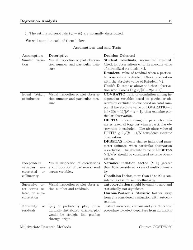
5. The estimated residuals (yi − yi) are normally distributed.
We will examine each of them below.
Assumptions and and Tests
Assumption Descriptive Decision OrientedSimilar varia-tion
Visual inspection or plot observa-tion number and particular mea-sure
Student residuals, normalized residual.Check for observations with the absolute valueof normalized residuals ≥ 2.Rstudent, value of residual when a particu-lar observation is deleted. Check observationwith the absolute value of Rstudent ≥2.Cook’s D, same as above and check observa-tion with Cook’s D ≥ 8/[N − 2(k + 1)].
Equal Weightor influence
Visual inspection or plot observa-tion number and particular mea-sure
COVRATIO, ratio of covariation among in-dependent variables based on particular ob-servation excluded to one based on total sam-ple. If the absolute value of COVARATIO−1is ≥ 3(k + 1)/[N − k − 1], then examine par-ticular observation.DFFITS indicate change in parameter esti-mates taken all together when a particular ob-servation is excluded. The absolute value ofDFFITS ≥ 2
√(k − 1)/N considered extreme
observation.DFBETAS indicate change individual para-meter estimate, when particular observationis excluded. The absolute value of DFBETAS≥ 2/
√N should be considered extreme obser-
vation.Independentvariables un-correlated orcollinearity
Visual inspection of correlationsand proportion of variance sharedacross variables.
Variance inflation factor (VIF) greaterthan 10 is considered a case of multicollinear-ity.Condition Index, more than 15 to 20 is con-sidered a case for multicollinearity.
Successive er-ror terms re-lated or auto-correlation
Visual inspection or plot observa-tion number and residuals.
autocorrelation should be equal to zero andstatistically not significant.Durbin-Watson’s Statistic farther awayfrom 2 is considered a situation with autocor-relation.
Normality ofresiduals
Q-Q or probability plot, for anormally distributed variable, plotwould be straight line passingthrough origin.
Tests of skewness, kurtosis and / or other testprocedure to detect departure from normality.
Multivariate Research Methods Course: COST*6060
Regression Analysis 13
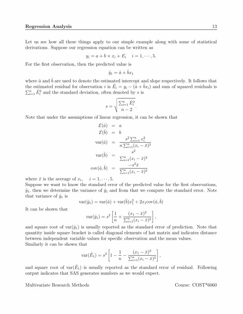
Let us see how all these things apply to our simple example along with some of statisticalderivations. Suppose our regression equation can be written as
yi = a + b × xi + Ei i = 1, · · · , 5.
For the first observation, then the predicted value is
y1 = a + bx1
where a and b are used to denote the estimated intercept and slope respectively. It follows thatthe estimated residual for observation i is Ei = yi − (a + bxi) and sum of squared residuals is∑n
i=1 E2i and the standard deviation, often denoted by s is
s =
√√√√∑n
i=1 E2i
n − 2.
Note that under the assumptions of linear regression, it can be shown that
E(a) = a
E(b) = b
var(a) =s2∑n
i=1 x2i
n∑n
i=1(xi − x)2
var(b) =s2
∑ni=1(xi − x)2
cov(a, b) =−s2x
∑ni=1(xi − x)2
where x is the average of xi, i = 1, · · · , 5.Suppose we want to know the standard error of the predicted value for the first observations,y1, then we determine the variance of y1 and from that we compute the standard error. Notethat variance of y1 is
var(y1) = var(a) + var(b)x21 + 2x1cov(a, b)
It can be shown that
var(y1) = s2
[1
n+
(x1 − x)2
∑ni=1(xi − x)2
],
and square root of var(y1) is usually reported as the standard error of prediction. Note thatquantity inside square bracket is called diagonal elements of hat matrix and indicates distancebetween independent variable values for specific observation and the mean values.Similarly it can be shown that
var(E1) = s2
[1 − 1
n− (x1 − x)2
∑ni=1(xi − x)2
],
and square root of var(E1) is usually reported as the standard error of residual. Followingoutput indicates that SAS generates numbers as we would expect.
Multivariate Research Methods Course: COST*6060
Regression Analysis 14
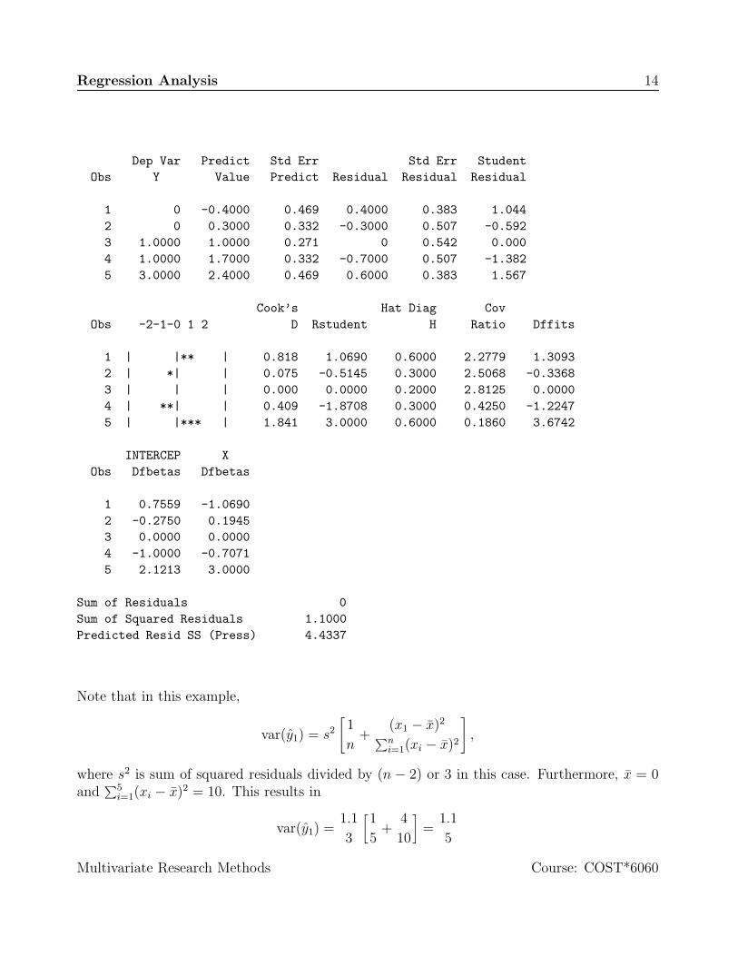
Dep Var Predict Std Err Std Err StudentObs Y Value Predict Residual Residual Residual
1 0 -0.4000 0.469 0.4000 0.383 1.0442 0 0.3000 0.332 -0.3000 0.507 -0.5923 1.0000 1.0000 0.271 0 0.542 0.0004 1.0000 1.7000 0.332 -0.7000 0.507 -1.3825 3.0000 2.4000 0.469 0.6000 0.383 1.567
Cook’s Hat Diag CovObs -2-1-0 1 2 D Rstudent H Ratio Dffits
1 | |** | 0.818 1.0690 0.6000 2.2779 1.30932 | *| | 0.075 -0.5145 0.3000 2.5068 -0.33683 | | | 0.000 0.0000 0.2000 2.8125 0.00004 | **| | 0.409 -1.8708 0.3000 0.4250 -1.22475 | |*** | 1.841 3.0000 0.6000 0.1860 3.6742
INTERCEP XObs Dfbetas Dfbetas
1 0.7559 -1.06902 -0.2750 0.19453 0.0000 0.00004 -1.0000 -0.70715 2.1213 3.0000
Sum of Residuals 0Sum of Squared Residuals 1.1000Predicted Resid SS (Press) 4.4337
Note that in this example,
var(y1) = s2
[1
n+
(x1 − x)2
∑ni=1(xi − x)2
],
where s2 is sum of squared residuals divided by (n − 2) or 3 in this case. Furthermore, x = 0and
∑5i=1(xi − x)2 = 10. This results in
var(y1) =1.1
3
[1
5+
4
10
]=
1.1
5
Multivariate Research Methods Course: COST*6060
Regression Analysis 15
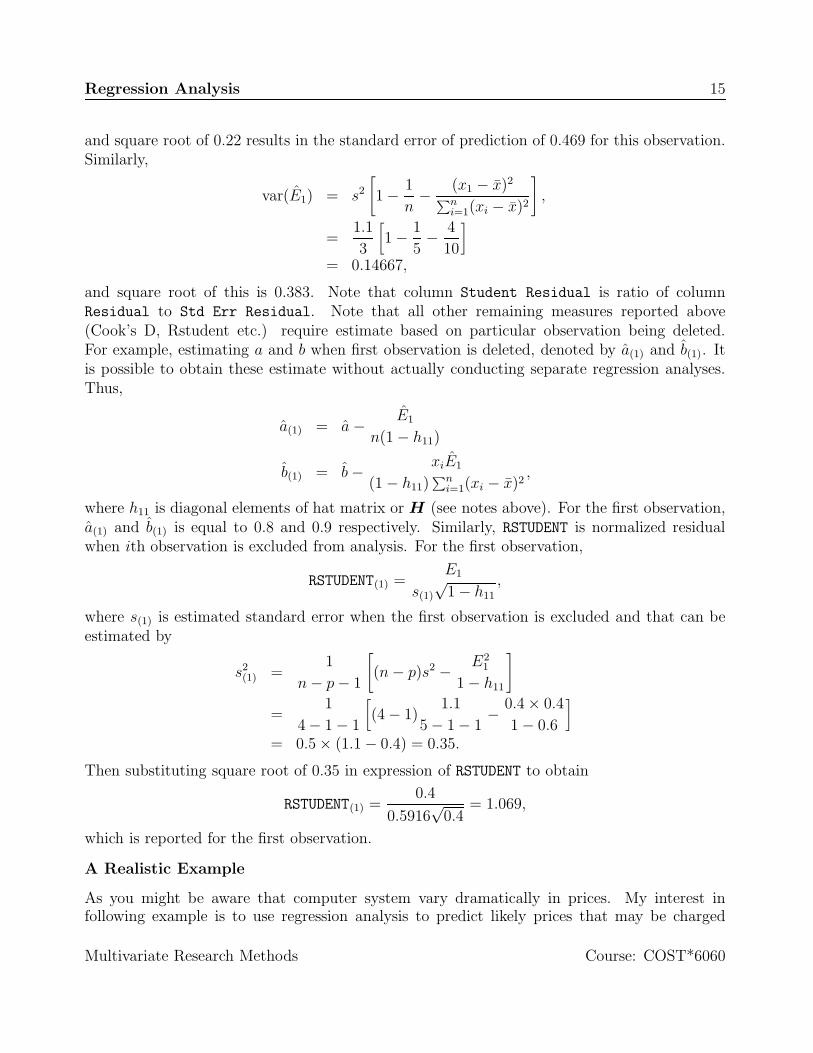
and square root of 0.22 results in the standard error of prediction of 0.469 for this observation.Similarly,
var(E1) = s2
[1 − 1
n− (x1 − x)2
∑ni=1(xi − x)2
],
=1.1
3
[1 − 1
5− 4
10
]
= 0.14667,
and square root of this is 0.383. Note that column Student Residual is ratio of columnResidual to Std Err Residual. Note that all other remaining measures reported above(Cook’s D, Rstudent etc.) require estimate based on particular observation being deleted.For example, estimating a and b when first observation is deleted, denoted by a(1) and b(1). Itis possible to obtain these estimate without actually conducting separate regression analyses.Thus,
a(1) = a − E1
n(1 − h11)
b(1) = b − xiE1
(1 − h11)∑n
i=1(xi − x)2,
where h11 is diagonal elements of hat matrix or H (see notes above). For the first observation,a(1) and b(1) is equal to 0.8 and 0.9 respectively. Similarly, RSTUDENT is normalized residualwhen ith observation is excluded from analysis. For the first observation,
RSTUDENT(1) =E1
s(1)
√1 − h11
,
where s(1) is estimated standard error when the first observation is excluded and that can beestimated by
s2(1) =
1
n − p − 1
[(n − p)s2 − E2
1
1 − h11
]
=1
4 − 1 − 1
[(4 − 1)
1.1
5 − 1 − 1− 0.4 × 0.4
1 − 0.6
]
= 0.5 × (1.1 − 0.4) = 0.35.
Then substituting square root of 0.35 in expression of RSTUDENT to obtain
RSTUDENT(1) =0.4
0.5916√
0.4= 1.069,
which is reported for the first observation.
A Realistic Example
As you might be aware that computer system vary dramatically in prices. My interest infollowing example is to use regression analysis to predict likely prices that may be charged
Multivariate Research Methods Course: COST*6060
Regression Analysis 16
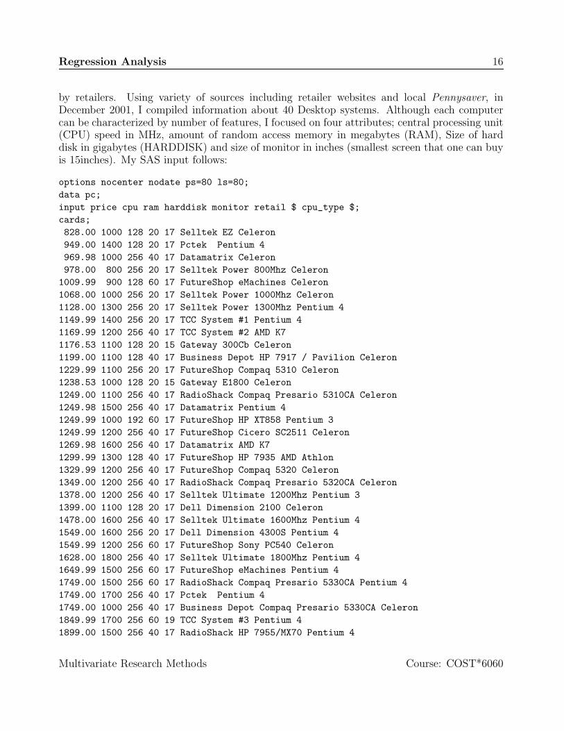
by retailers. Using variety of sources including retailer websites and local Pennysaver, inDecember 2001, I compiled information about 40 Desktop systems. Although each computercan be characterized by number of features, I focused on four attributes; central processing unit(CPU) speed in MHz, amount of random access memory in megabytes (RAM), Size of harddisk in gigabytes (HARDDISK) and size of monitor in inches (smallest screen that one can buyis 15inches). My SAS input follows:
options nocenter nodate ps=80 ls=80;data pc;input price cpu ram harddisk monitor retail $ cpu_type $;cards;828.00 1000 128 20 17 Selltek EZ Celeron949.00 1400 128 20 17 Pctek Pentium 4969.98 1000 256 40 17 Datamatrix Celeron978.00 800 256 20 17 Selltek Power 800Mhz Celeron
1009.99 900 128 60 17 FutureShop eMachines Celeron1068.00 1000 256 20 17 Selltek Power 1000Mhz Celeron1128.00 1300 256 20 17 Selltek Power 1300Mhz Pentium 41149.99 1400 256 20 17 TCC System #1 Pentium 41169.99 1200 256 40 17 TCC System #2 AMD K71176.53 1100 128 20 15 Gateway 300Cb Celeron1199.00 1100 128 40 17 Business Depot HP 7917 / Pavilion Celeron1229.99 1100 256 20 17 FutureShop Compaq 5310 Celeron1238.53 1000 128 20 15 Gateway E1800 Celeron1249.00 1100 256 40 17 RadioShack Compaq Presario 5310CA Celeron1249.98 1500 256 40 17 Datamatrix Pentium 41249.99 1000 192 60 17 FutureShop HP XT858 Pentium 31249.99 1200 256 40 17 FutureShop Cicero SC2511 Celeron1269.98 1600 256 40 17 Datamatrix AMD K71299.99 1300 128 40 17 FutureShop HP 7935 AMD Athlon1329.99 1200 256 40 17 FutureShop Compaq 5320 Celeron1349.00 1200 256 40 17 RadioShack Compaq Presario 5320CA Celeron1378.00 1200 256 40 17 Selltek Ultimate 1200Mhz Pentium 31399.00 1100 128 20 17 Dell Dimension 2100 Celeron1478.00 1600 256 40 17 Selltek Ultimate 1600Mhz Pentium 41549.00 1600 256 20 17 Dell Dimension 4300S Pentium 41549.99 1200 256 60 17 FutureShop Sony PC540 Celeron1628.00 1800 256 40 17 Selltek Ultimate 1800Mhz Pentium 41649.99 1500 256 60 17 FutureShop eMachines Pentium 41749.00 1500 256 60 17 RadioShack Compaq Presario 5330CA Pentium 41749.00 1700 256 40 17 Pctek Pentium 41749.00 1000 256 40 17 Business Depot Compaq Presario 5330CA Celeron1849.99 1700 256 60 19 TCC System #3 Pentium 41899.00 1500 256 40 17 RadioShack HP 7955/MX70 Pentium 4
Multivariate Research Methods Course: COST*6060
Regression Analysis 17
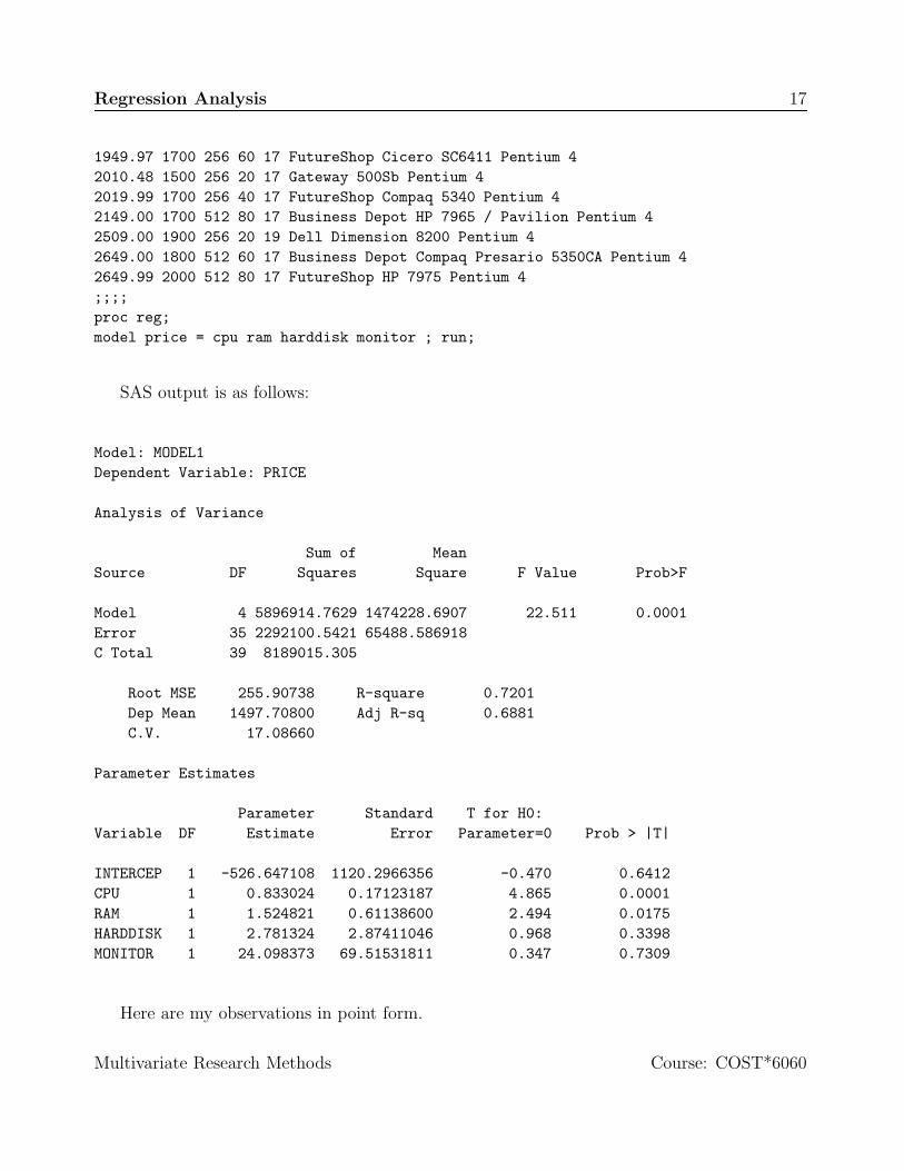
1949.97 1700 256 60 17 FutureShop Cicero SC6411 Pentium 42010.48 1500 256 20 17 Gateway 500Sb Pentium 42019.99 1700 256 40 17 FutureShop Compaq 5340 Pentium 42149.00 1700 512 80 17 Business Depot HP 7965 / Pavilion Pentium 42509.00 1900 256 20 19 Dell Dimension 8200 Pentium 42649.00 1800 512 60 17 Business Depot Compaq Presario 5350CA Pentium 42649.99 2000 512 80 17 FutureShop HP 7975 Pentium 4;;;;proc reg;model price = cpu ram harddisk monitor ; run;
SAS output is as follows:
Model: MODEL1Dependent Variable: PRICE
Analysis of Variance
Sum of MeanSource DF Squares Square F Value Prob>F
Model 4 5896914.7629 1474228.6907 22.511 0.0001Error 35 2292100.5421 65488.586918C Total 39 8189015.305
Root MSE 255.90738 R-square 0.7201Dep Mean 1497.70800 Adj R-sq 0.6881C.V. 17.08660
Parameter Estimates
Parameter Standard T for H0:Variable DF Estimate Error Parameter=0 Prob > |T|
INTERCEP 1 -526.647108 1120.2966356 -0.470 0.6412CPU 1 0.833024 0.17123187 4.865 0.0001RAM 1 1.524821 0.61138600 2.494 0.0175HARDDISK 1 2.781324 2.87411046 0.968 0.3398MONITOR 1 24.098373 69.51531811 0.347 0.7309
Here are my observations in point form.
Multivariate Research Methods Course: COST*6060
Regression Analysis 18
• The null hypothesis states that variation in price can not be explained by CPU speed,amount RAM, size of hard disk and size of monitor. We reject this hypothesis, becauseprobability of F-statistic is less than or equal to 0.05.
• We are explaining about 72% of variation in price by these four variables.
• Regression equation can be written as
Price = −526.65 + 0.833 × CPU + 1.525 × RAM
+ 2.781 × HARDDISK + 24.098 × MONITOR.
• Note that the parameter associated with variables CPU and RAM have correct signs4
and statistically significant (probability of t-statistic is less than 0.05).
• The parameters associated with variables HARDDISK and MONITOR have correct signbut statistically not significant. That means, these parameters could be equal to zero.
• Consider a desktop with 1 Ghz, with 256 Megabytes of RAM, about 40 gigabytes harddrive and 17 inches MONITOR. For such machine, I should be expected to pay about$1,218. This is concluded as follows:
Price = −526.65 + 0.833 × 1000 + 1.525 × 256 + 2.781 × 40 + 24.098 × 17.
= −526.65 + 833 + 390.4 + 111.24 + 409.67
= 1217.66
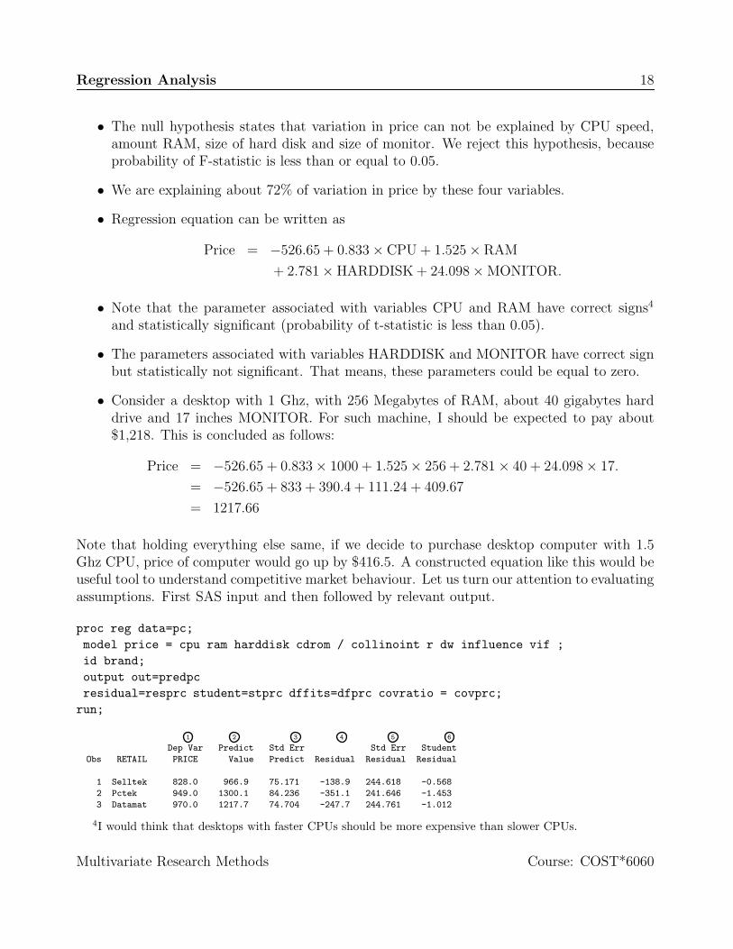
Note that holding everything else same, if we decide to purchase desktop computer with 1.5Ghz CPU, price of computer would go up by $416.5. A constructed equation like this would beuseful tool to understand competitive market behaviour. Let us turn our attention to evaluatingassumptions. First SAS input and then followed by relevant output.
proc reg data=pc;model price = cpu ram harddisk cdrom / collinoint r dw influence vif ;id brand;output out=predpcresidual=resprc student=stprc dffits=dfprc covratio = covprc;
run;
1 2 3 4 5 6
Dep Var Predict Std Err Std Err Student
Obs RETAIL PRICE Value Predict Residual Residual Residual
1 Selltek 828.0 966.9 75.171 -138.9 244.618 -0.568
2 Pctek 949.0 1300.1 84.236 -351.1 241.646 -1.453
3 Datamat 970.0 1217.7 74.704 -247.7 244.761 -1.012
4I would think that desktops with faster CPUs should be more expensive than slower CPUs.
Multivariate Research Methods Course: COST*6060
Regression Analysis 19
4 Selltek 978.0 995.4 117.797 -17.4251 227.184 -0.077
5 FutureS 1010.0 994.8 125.129 15.1867 223.229 0.068
6 Selltek 1068.0 1162.0 92.814 -94.0298 238.483 -0.394
7 Selltek 1128.0 1411.9 71.552 -283.9 245.701 -1.156
8 TCC 1150.0 1495.2 71.607 -345.2 245.685 -1.405
9 TCC 1170.0 1384.3 49.600 -214.3 251.055 -0.853
10 Gateway 1176.5 1002.0 142.267 174.6 212.718 0.821
11 Busines 1199.0 1105.8 77.940 93.2184 243.750 0.382
12 FutureS 1230.0 1245.3 82.844 -15.3422 242.127 -0.063
13 Gateway 1238.5 918.7 138.660 319.9 215.086 1.487
14 RadioSh 1249.0 1301.0 61.051 -51.9587 248.518 -0.209
15 Datamat 1250.0 1634.2 46.662 -384.2 251.617 -1.527
16 FutureS 1250.0 1175.7 101.098 74.2958 235.091 0.316
17 FutureS 1250.0 1384.3 49.600 -134.3 251.055 -0.535
18 Datamat 1270.0 1717.5 57.060 -447.5 249.465 -1.794
19 FutureS 1300.0 1272.4 81.196 27.6037 242.685 0.114
20 FutureS 1330.0 1384.3 49.600 -54.2711 251.055 -0.216
21 RadioSh 1349.0 1384.3 49.600 -35.2611 251.055 -0.140
22 Selltek 1378.0 1384.3 49.600 -6.2611 251.055 -0.025
23 Dell 1399.0 1050.2 71.640 348.8 245.675 1.420
24 Selltek 1478.0 1717.5 57.060 -239.5 249.465 -0.960
25 Dell 1549.0 1661.8 83.082 -112.8 242.045 -0.466
26 FutureS 1550.0 1439.9 76.358 110.1 244.250 0.451
27 Selltek 1628.0 1884.1 84.689 -256.1 241.488 -1.060
28 FutureS 1650.0 1689.8 72.395 -39.8047 245.454 -0.162
29 RadioSh 1749.0 1689.8 72.395 59.2053 245.454 0.241
30 Pctek 1749.0 1800.8 70.148 -51.7730 246.105 -0.210
31 Busines 1749.0 1217.7 74.704 531.3 244.761 2.171
32 TCC 1850.0 1904.6 144.629 -54.6063 211.118 -0.259
33 RadioSh 1899.0 1634.2 46.662 264.8 251.617 1.053
34 FutureS 1950.0 1856.4 88.206 93.5705 240.226 0.390
35 Gateway 2010.5 1578.5 75.643 431.9 244.472 1.767
36 FutureS 2020.0 1800.8 70.148 219.2 246.105 0.891
37 Busines 2149.0 2302.4 134.871 -153.4 217.482 -0.705
38 Dell 2509.0 1959.9 160.628 549.1 199.216 2.756
39 Busines 2649.0 2330.1 128.694 318.9 221.193 1.442
40 FutureS 2650.0 2552.3 136.722 97.7026 216.323 0.452
1 column is values of dependent variable (yi). This variable is sorted in ascending order to helpus interpret other statistical measures.
2 column is predicted values for dependent variable (yi). For the first observation,
y1 = −526.65 + 0.833 × 1000 + 1.525 × 128 + 2.781 × 20 + 24.098 × 17 = 966.9.
3 column is the standard error associated with predicted values, a larger number indicates thatvalues of independent variables are farther away from the “average” observation. For the firstobservation independent variable vector, x1 is [110001282017]. Then Var(y1) = s2x′
1(X′X)−1x.
4 column is residual or error values, (yi − yi).
5 column is the standard error associated with error, and again a larger number indicates thatvalues of independent variables are farther away from the “average” observation.
6 column the Student residuals are also called normalized (generally normalized means divided bythe standard error) residuals. If residuals are normally distributed then normalized residualsmore than 2 should be considered extreme observations.
Multivariate Research Methods Course: COST*6060
Regression Analysis 20
7 8 9 10 11
Cook’s Hat Diag Cov
Obs RETAIL -2-1-0 1 2 D Rstudent H Ratio
1 Selltek | *| | 0.006 -0.5621 0.0863 1.2080
2 Pctek | **| | 0.051 -1.4771 0.1083 0.9499
3 Datamat | **| | 0.019 -1.0123 0.0852 1.0893
4 Selltek | | | 0.000 -0.0756 0.2119 1.4655
5 FutureS | | | 0.000 0.0671 0.2391 1.5182
6 Selltek | | | 0.005 -0.3895 0.1315 1.3018
7 Selltek | **| | 0.023 -1.1614 0.0782 1.0323
8 TCC | **| | 0.034 -1.4258 0.0783 0.9381
9 TCC | *| | 0.006 -0.8501 0.0376 1.0812
10 Gateway | |* | 0.060 0.8168 0.3091 1.5181
11 Busines | | | 0.003 0.3777 0.0928 1.2478
12 FutureS | | | 0.000 -0.0625 0.1048 1.2906
13 Gateway | |** | 0.184 1.5144 0.2936 1.1807
14 RadioSh | | | 0.001 -0.2062 0.0569 1.2181
15 Datamat | ***| | 0.016 -1.5577 0.0332 0.8471
16 FutureS | | | 0.004 0.3119 0.1561 1.3503
17 FutureS | *| | 0.002 -0.5293 0.0376 1.1528
18 Datamat | ***| | 0.034 -1.8553 0.0497 0.7511
19 FutureS | | | 0.000 0.1121 0.1007 1.2830
20 FutureS | | | 0.000 -0.2132 0.0376 1.1931
21 RadioSh | | | 0.000 -0.1385 0.0376 1.1977
22 Selltek | | | 0.000 -0.0246 0.0376 1.2010
23 Dell | |** | 0.034 1.4417 0.0784 0.9323
24 Selltek | *| | 0.010 -0.9588 0.0497 1.0645
25 Dell | | | 0.005 -0.4609 0.1054 1.2525
26 FutureS | | | 0.004 0.4456 0.0890 1.2325
27 Selltek | **| | 0.028 -1.0624 0.1095 1.1026
28 FutureS | | | 0.000 -0.1599 0.0800 1.2518
29 RadioSh | | | 0.001 0.2379 0.0800 1.2461
30 Pctek | | | 0.001 -0.2075 0.0751 1.2420
31 Busines | |**** | 0.088 2.3001 0.0852 0.6132
32 TCC | | | 0.006 -0.2552 0.3194 1.6823
33 RadioSh | |** | 0.008 1.0542 0.0332 1.0181
34 FutureS | | | 0.004 0.3847 0.1188 1.2836
35 Gateway | |*** | 0.060 1.8247 0.0874 0.7939
36 FutureS | |* | 0.013 0.8881 0.0751 1.1145
37 Busines | *| | 0.038 -0.7001 0.2778 1.4900
38 Dell | |***** | 0.988 3.0699 0.3940 0.5613
39 Busines | |** | 0.141 1.4654 0.2529 1.1392
40 FutureS | | | 0.016 0.4465 0.2854 1.5711
7 column is a plot of normalized residuals and these numbers generally vary between −2 and 2.
8 column Cook’s D is a summary measure of the influence of a single observation on the totalchanges in all other residuals when observation is excluded from the estimation. In our case,Cook’s D ≥ 8
N−2(k+1) is 840−10 or 0.267 would be considered influential observation (see obser-
vation number 38).
9 column Rstudent is similar to Cook’s D with the exception that error variances are estimatedusing without the ith observation.
10 column Hat Diag H (Diagonal of Hat matrix H, also sometimes denoted as hii) is a ratioof variability for an observation to the sample variability in independent variables. If eachobservation has equal influence on regression equation, then the average influence would be
Multivariate Research Methods Course: COST*6060
Regression Analysis 21
k/N and observation with hii ≥ 2k/N ( 2×4/40 or 0.2 for our example) would be considered aninfluential observation. There are number of observations with such problem, especially towardsthe end of dataset or higher priced desktop systems.
11 column Cov ratio (Covariance ratio) is a ratio covariances when ith observation is excluded tothe sample covariances. A value of COVRATIO close to 1 indicates the “average” influence byan observation while the absolute value of (COVRATIO - 1) ≥ 3(k+1)
N−k−1 is considered significant
influential observation. For our case, COVRATIO ≥ 1 + (3×5)35 or 1.429 would be observations
with higher than the normal influence.
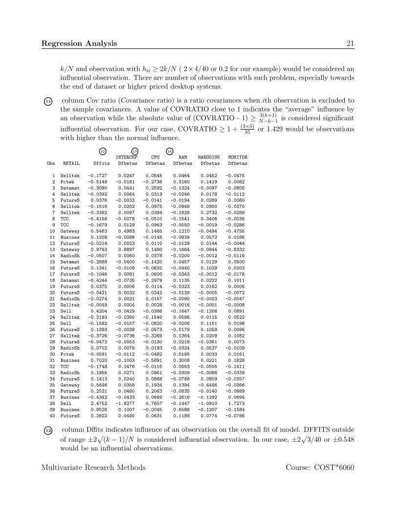
12 13 14
INTERCEP CPU RAM HARDDISK MONITOR
Obs RETAIL Dffits Dfbetas Dfbetas Dfbetas Dfbetas Dfbetas
1 Selltek -0.1727 0.0247 0.0545 0.0464 0.0452 -0.0475
2 Pctek -0.5149 -0.0181 -0.2738 0.3160 0.1419 0.0082
3 Datamat -0.3090 0.0441 0.2592 -0.1324 -0.0097 -0.0805
4 Selltek -0.0392 0.0064 0.0313 -0.0246 0.0178 -0.0112
5 FutureS 0.0376 -0.0033 -0.0141 -0.0194 0.0289 0.0060
6 Selltek -0.1516 0.0202 0.0975 -0.0948 0.0900 -0.0370
7 Selltek -0.3382 0.0097 0.0394 -0.1628 0.2732 -0.0289
8 TCC -0.4156 -0.0079 -0.0510 -0.1541 0.3406 -0.0035
9 TCC -0.1679 0.0129 0.0963 -0.0550 -0.0019 -0.0286
10 Gateway 0.5463 0.4983 0.1465 -0.1210 -0.0494 -0.4755
11 Busines 0.1208 -0.0088 -0.0148 -0.0839 0.0572 0.0186
12 FutureS -0.0214 0.0023 0.0110 -0.0129 0.0144 -0.0044
13 Gateway 0.9763 0.8897 0.1480 -0.1664 -0.0844 -0.8332
14 RadioSh -0.0507 0.0060 0.0378 -0.0200 -0.0012 -0.0116
15 Datamat -0.2889 -0.0400 -0.1420 0.0457 0.0129 0.0500
16 FutureS 0.1341 -0.0109 -0.0632 -0.0440 0.1029 0.0203
17 FutureS -0.1046 0.0081 0.0600 -0.0343 -0.0012 -0.0178
18 Datamat -0.4244 -0.0735 -0.2979 0.1135 0.0222 0.1011
19 FutureS 0.0375 0.0006 0.0114 -0.0323 0.0162 0.0005
20 FutureS -0.0421 0.0032 0.0242 -0.0138 -0.0005 -0.0072
21 RadioSh -0.0274 0.0021 0.0157 -0.0090 -0.0003 -0.0047
22 Selltek -0.0049 0.0004 0.0028 -0.0016 -0.0001 -0.0008
23 Dell 0.4204 -0.0429 -0.0386 -0.1647 -0.1206 0.0891
24 Selltek -0.2193 -0.0380 -0.1540 0.0586 0.0115 0.0522
25 Dell -0.1582 -0.0157 -0.0820 -0.0206 0.1151 0.0198
26 FutureS 0.1393 -0.0039 -0.0573 -0.0179 0.1059 0.0096
27 Selltek -0.3726 -0.0736 -0.3269 0.1364 0.0209 0.1082
28 FutureS -0.0472 -0.0053 -0.0130 0.0218 -0.0361 0.0073
29 RadioSh 0.0702 0.0079 0.0193 -0.0324 0.0537 -0.0109
30 Pctek -0.0591 -0.0112 -0.0482 0.0195 0.0033 0.0161
31 Busines 0.7020 -0.1003 -0.5891 0.3008 0.0221 0.1828
32 TCC -0.1748 0.1476 -0.0115 0.0553 -0.0555 -0.1411
33 RadioSh 0.1955 0.0271 0.0961 -0.0309 -0.0088 -0.0339
34 FutureS 0.1413 0.0240 0.0868 -0.0788 0.0859 -0.0357
35 Gateway 0.5646 0.0358 0.1934 0.1394 -0.4446 -0.0366
36 FutureS 0.2531 0.0480 0.2063 -0.0835 -0.0140 -0.0689
37 Busines -0.4342 -0.0433 0.0669 -0.2616 -0.1292 0.0694
38 Dell 2.4752 -1.8277 0.7657 -0.1447 -1.0910 1.7273
39 Busines 0.8526 0.1007 -0.0045 0.6588 -0.1207 -0.1584
40 FutureS 0.2822 0.0490 0.0631 0.1189 0.0774 -0.0786
12 column Dffits indicates influence of an observation on the overall fit of model. DFFITS outsideof range ±2
√(k − 1)/N is considered influential observation. In our case, ±2
√3/40 or ±0.548
would be an influential observations.
Multivariate Research Methods Course: COST*6060
Regression Analysis 22
13 14 columns DFBETAs indicate influence of particular observation on a specific parameterestimate. Observations outside ±2/
√N would influencing particular observations. In our case,
the appropriate range is ±2/√
40 or ±0.316. There will one DFBETA for each parameterestimated. In our case there are five such measures.
15
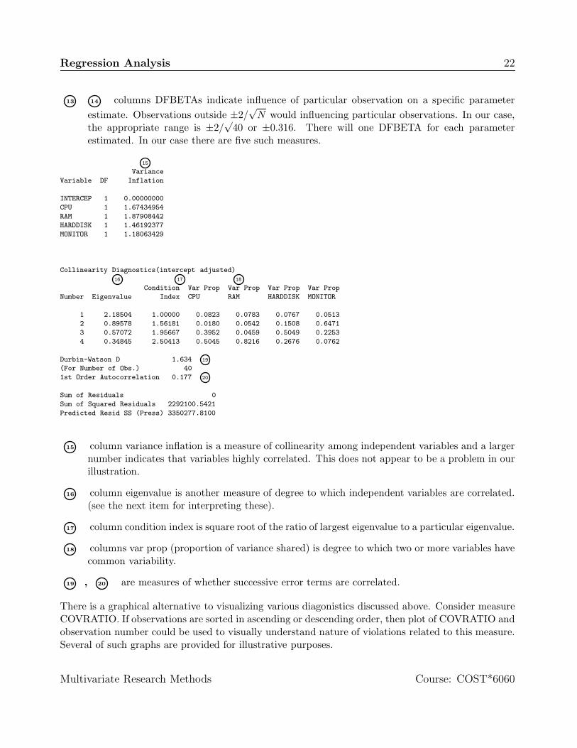
Variance
Variable DF Inflation
INTERCEP 1 0.00000000
CPU 1 1.67434954
RAM 1 1.87908442
HARDDISK 1 1.46192377
MONITOR 1 1.18063429
Collinearity Diagnostics(intercept adjusted)
16 17 18
Condition Var Prop Var Prop Var Prop Var Prop
Number Eigenvalue Index CPU RAM HARDDISK MONITOR
1 2.18504 1.00000 0.0823 0.0783 0.0767 0.0513
2 0.89578 1.56181 0.0180 0.0542 0.1508 0.6471
3 0.57072 1.95667 0.3952 0.0459 0.5049 0.2253
4 0.34845 2.50413 0.5045 0.8216 0.2676 0.0762
Durbin-Watson D 1.634 19
(For Number of Obs.) 40
1st Order Autocorrelation 0.177 20
Sum of Residuals 0
Sum of Squared Residuals 2292100.5421
Predicted Resid SS (Press) 3350277.8100
15 column variance inflation is a measure of collinearity among independent variables and a largernumber indicates that variables highly correlated. This does not appear to be a problem in ourillustration.
16 column eigenvalue is another measure of degree to which independent variables are correlated.(see the next item for interpreting these).
17 column condition index is square root of the ratio of largest eigenvalue to a particular eigenvalue.
18 columns var prop (proportion of variance shared) is degree to which two or more variables havecommon variability.
19 , 20 are measures of whether successive error terms are correlated.
There is a graphical alternative to visualizing various diagonistics discussed above. Consider measureCOVRATIO. If observations are sorted in ascending or descending order, then plot of COVRATIO andobservation number could be used to visually understand nature of violations related to this measure.Several of such graphs are provided for illustrative purposes.
Multivariate Research Methods Course: COST*6060
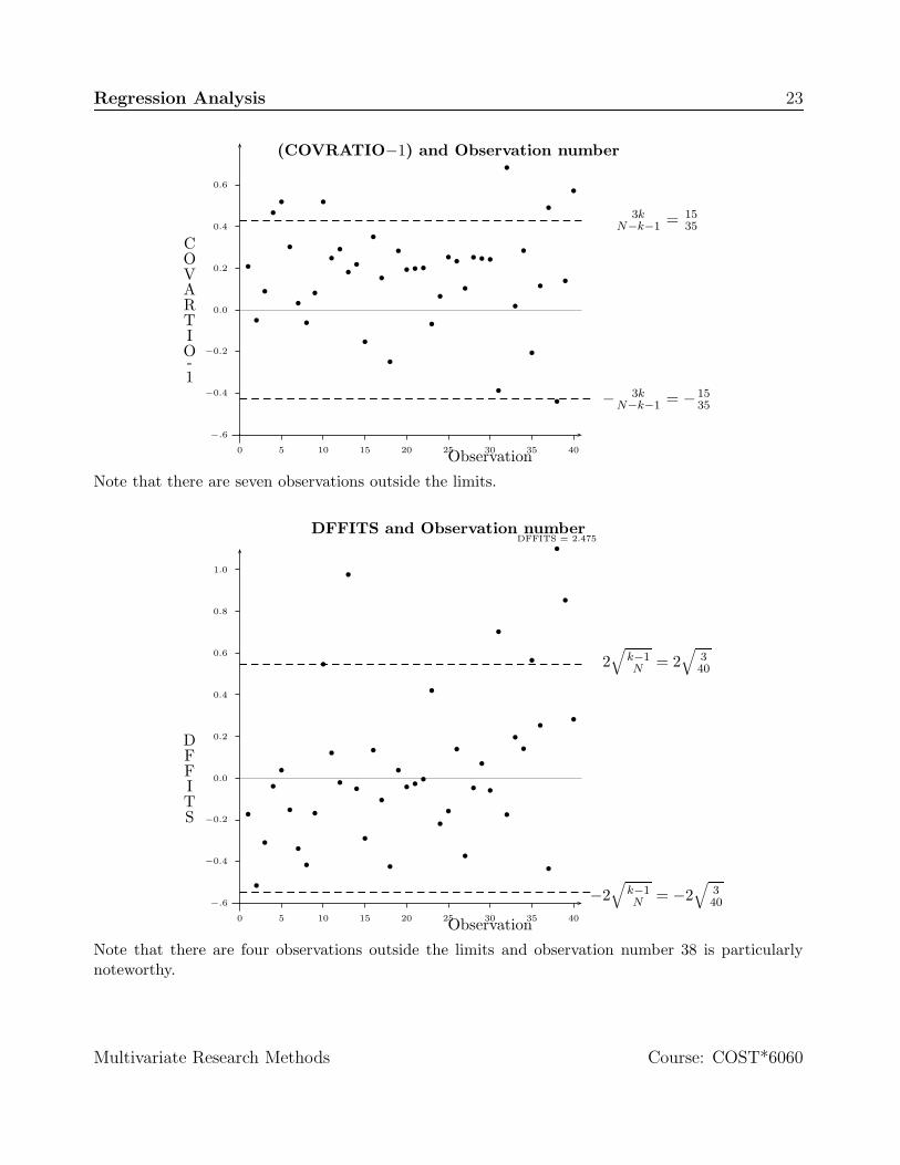
Regression Analysis 23
0 5 10 15 20 25 30 35 40
−.6
−0.4
−0.2
0.0
0.2
0.4
0.6
b
b
b
b
b
b
b
b
b
b
b
b
b
b
b
b
b
b
b
b b b
b
b
bb
b
b b b
b
b
b
b
b
b
b
b
b
b
3kN−k−1 = 15
35
− 3kN−k−1 = −15
35
Observation
COVARTIO-1
(COVRATIO−1) and Observation number
Note that there are seven observations outside the limits.
0 5 10 15 20 25 30 35 40
−.6
−0.4
−0.2
0.0
0.2
0.4
0.6
0.8
1.0
b
b
b
b
b
b
b
b
b
b
b
b
b
b
b
b
b
b
b
bbb
b
b
b
b
b
b
b
b
b
b
b
b
b
b
b
b
b
b
DFFITS = 2.475
2√
k−1N = 2
√340
−2√
k−1N = −2
√340
Observation
DFFITS
DFFITS and Observation number
Note that there are four observations outside the limits and observation number 38 is particularlynoteworthy.
Multivariate Research Methods Course: COST*6060
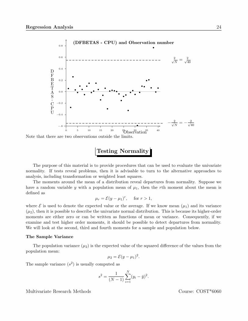
Regression Analysis 24
0 5 10 15 20 25 30 35 40
−.6
−0.4
−0.2
0.0
0.2
0.4
0.6
0.8
b
b
b
b
b
b
b
b
b
b
bb
b
b
b
b
b
b
bb b
b
b
b
bb
b
b
b
b
b
b
b b
bb
b
b
b
b
2√N
= 2√40
− 2√N
= − 2√40
Observation
DFBETAS-CPU
(DFBETAS - CPU) and Observation number
Note that there are two observations outside the limits.
Testing Normality
The purpose of this material is to provide procedures that can be used to evaluate the univariatenormality. If tests reveal problems, then it is advisable to turn to the alternative approaches toanalysis, including transformation or weighted least squares.
The moments around the mean of a distribution reveal departures from normality. Suppose wehave a random variable y with a population mean of µ1, then the rth moment about the mean isdefined as
µr = E(y − µ1)r, for r > 1,
where E is used to denote the expected value or the average. If we know mean (µ1) and its variance(µ2), then it is possible to describe the univariate normal distribution. This is because its higher-ordermoments are either zero or can be written as functions of mean or variance. Consequently, if weexamine and test higher order moments, it should be possible to detect departures from normality.We will look at the second, third and fourth moments for a sample and population below.
The Sample Variance
The population variance (µ2) is the expected value of the squared difference of the values from thepopulation mean:
µ2 = E(y − µ1)2.
The sample variance (s2) is usually computed as
s2 =1
(N − 1)
N∑
i=1
(yi − y)2.
Multivariate Research Methods Course: COST*6060
Regression Analysis 25
Test of Skewness to Detect Non-normality
Skewness is a measure of the tendency of the deviations to be larger in one direction than in the other.
A population skewness is defined asE(y − µ1)3
µ3/22
.
The sample third moment (g1) is computed as5
g1 =N
(N − 1)(N − 2)
∑Ni=1(yi − y)3
s3.
The coefficient of skewness (CS) or√
b1 is
CS =√
b1 =N − 2√
N(N − 1)g1.
For a normally distributed variable, CS is 0. Moreover, if CS is negative and statistically significant,then skew is to the left. On the other hand, if CS is positive, then skew is to the right. In the largesamples, hypothesis test for CS can be performed by converting CS as a unit normal deviate. That is,
z√b1= ±
√CS(N + 1)(N + 3)
6(N − 2)
where the undetermined sign is the same as that of the third moment and this quantity is approximatelynormally distributed under the null hypothesis of population normality.
Tests of Kurtosis to Detect Non-Normality
The heaviness of the tails is measured by kurtosis or the coefficient of kurtosis (b2). The populationkurtosis is defined as
µ4 =E(y − µ1)4
µ22
− 3.
The sample fourth moment is calculated as
g2 =N(N + 1)
(N − 1)(N − 2)(N − 3)
∑Ni=1(yi − y)4
s4− 3(N − 1)2
(N − 2)(N − 3).
To convert fourth moment to kurtosis (b2) we need to compute
b2 = 3N − 1N + 1
+(N − 2)(N − 3)(N + 1)(N − 1)
g2.
For a normally distributed variable, b2 is equal to 3. In large samples, hypothesis test for b2 can beperformed by converting b2 as a unit normal deviate. That is,
zb2 =[b2 +
6(N + 1)
]√(N + 1)2(N + 3)(N + 5)24N(N − 2)(N − 3)
.
5PROC UNIVARIATE in SAS reports the third and fourth moments but not coefficent of skewness andkurtosis as indicated below.
Multivariate Research Methods Course: COST*6060
Regression Analysis 26
and this estimate is approximately normally distributed under the null hypothesis of population nor-mality. Note that values less than zero indicate that the distribution is more peaked with longer tailsthan the normal distribution; values greater than zero indicate flatter distribution in the centre andwith shorter tails than the normal distribution.Omnibus Tests of Normality
It is possible to combine test of skewness and kurtosis into one test that detects departure fromnormality due to either of these measures. Such tests are called omnibus. The test statistic
K2 = z2√b1
+ z2b2
where the K2 statistic has approximately a chi-square (χ2) distribution, with 2 degrees of freedomwhen the population is normally distributed.
There are many other tests to determine departure of a variable from normality. The programNORMTEST also prints statistic called Shapiro-Wilk test6. It is based on assumption that orderedobservations of normally distributed variable will have equal and similar weights. Thus, if weightassigned to the first observation (the lowest value of yi, let us call it y(1)) is 1/N and the secondobservation (one that is more than or equal to y(1), let us call it y(2)) will have weight of 2/N and soon7. The test statistic of Shapiro-Wilk (W) is
W =
∑Ni=1
(aiy(i)
)2
∑Ni=1 (yi − y)2
where ai is weight associated with i observation and variable y is ordered such that y(1) ≤ y(2) ≤ · · · ≤y(N). Small values of W correspond to departure from normality.
We will examine below SAS input and output to conduct these tests. As you have seen above,numerical calculations involved in above are extensive. To assist you with these calculations, I have aSAS macro8 To access this macro, I would use following SAS input.
%include "c:\sas6_12\normtest.sas";%normtest(stprc,predpc);
In this instance predpc is name of SAS dataset and stprc is a variable whose normality is beingtested. SAS will produce two sorts of outputs; one graphical and another textual. These follow here.First SAS and then graphical output.
Normality Test for variable stprc N=40
6Shapiro, S. S. and Wilk M. B. (1965) “A analysis of variance test for Normality”, Biometrika, vol. 52,591–611.
7This is intuitive description of the statistic and not the exact method.8This macro is modified version of as it appeared in American Statistician and it was originally written
by D’Agostino Ralph B., Albert Belanger and Ralph B. D’Agostino Jr. (1990) “A Suggestion for Using Pow-erful and informative Tests of Normality”, Vol. 44, pp. 316–321. The macro for your usage is kept in fileG:\courses\COST6060\NORMTEST.SAS.
Multivariate Research Methods Course: COST*6060
Regression Analysis 27
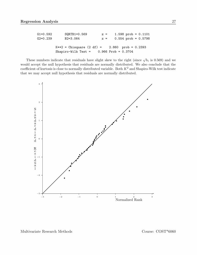
G1=0.592 SQRTB1=0.569 z = 1.598 prob = 0.1101G2=0.239 B2=3.064 z = 0.554 prob = 0.5798
K**2 = Chisquare (2 df) = 2.860 prob = 0.2393Shapiro-Wilk Test = 0.966 Prob = 0.3704
These numbers indicate that residuals have slight skew to the right (since√
b1 is 0.569) and wewould accept the null hypothesis that residuals are normally distributed. We also conclude that thecoefficient of kurtosis is close to normally distributed variable. Both K2 and Shapiro-Wilk test indicatethat we may accept null hypothesis that residuals are normally distributed.
−3 −2 −1 0 1 2 3
−3
−2
−1
0
1
2
3
b
b
b
b
b
b
b
b
b
b
b
b
b
b
b
b
b
b
b
b
b
b
b
b
b
b
b
b
b
b
b
b
b
b
b
b
b
b
b
b
Normalized Rank
Standardized
Residual
Multivariate Research Methods Course: COST*6060
Regression Analysis 28
Revise Model to meet Assumptions
• Failure of Similar variation or equal influence
1. Transform dependent variable, or independent variable or both.
2. Exclude observations with more influence.
3. Apply weighting scheme that are managerially or statistically meaningful.
4. Estimate model with weighted least squares or the least absolute deviation.
• Presence of Collinearity
1. Create new index variables that may capture correlations among independent variableseither conceptually (for example SES, instead income, occupation and education etc.)
2. Determine stability of parameters by excluding one or more variables.
3. Use statistical procedures for dealing with this problem, for example, transformation,alternative criterion to minimize.
• Lack of Independence of successive error values
1. May be caused by missing variables, competitive variables or customer loyalty, then includemissing variables.
2. Re-estimate model with autocorrelated errors.
• Error values not normally distributed
1. Use non-normal distribution to estimate parameters.
2. Use transformation convert dependent variable so that new variable is normally distributed.
3. Break sample in subsegments and estimate parameters for each subsegment.
Validate Revised Model
1. Use limited number of explanatory variables. Avoid using all variables to be included in yourregression model. If there are large number of variables, then create indices, groupings withconceptual idea. Then, use selected such variables to estimate models.
2. Use a large sample, 40 - 50 observations per variable included will have better stability toestimates than 5 - 10 observations.
3. Validate your model with hold-out or split-half sample or new sample.
Multivariate Research Methods Course: COST*6060
Regression Analysis 29
Limitations of Regression Analysis
• Moderating effects of variables
1. By group differences,
2. Interaction effects,
3. Effect occur only at certain level.
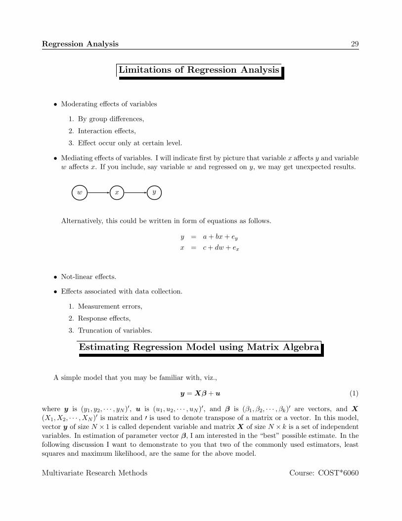
• Mediating effects of variables. I will indicate first by picture that variable x affects y and variablew affects x. If you include, say variable w and regressed on y, we may get unexpected results.
w x y
Alternatively, this could be written in form of equations as follows.
y = a + bx + ey
x = c + dw + ex
• Not-linear effects.
• Effects associated with data collection.
1. Measurement errors,
2. Response effects,
3. Truncation of variables.
Estimating Regression Model using Matrix Algebra
A simple model that you may be familiar with, viz.,
y = Xβ + u (1)
where y is (y1, y2, · · · , yN )′, u is (u1, u2, · · · , uN )′, and β is (β1, β2, · · · , βk)′ are vectors, and X(X1,X2, · · · ,XN )′ is matrix and ′ is used to denote transpose of a matrix or a vector. In this model,vector y of size N × 1 is called dependent variable and matrix X of size N × k is a set of independentvariables. In estimation of parameter vector β, I am interested in the “best” possible estimate. In thefollowing discussion I want to demonstrate to you that two of the commonly used estimators, leastsquares and maximum likelihood, are the same for the above model.
Multivariate Research Methods Course: COST*6060
Regression Analysis 30
Least Squares Estimator
In the least squares method, I want to find β of the regression parameter β so as to minimize the sumof squared residuals. Mathematically I may write
Minimize f(β) = (y − Xβ)′(y − Xβ) (2)= y′y − 2y′Xβ + β′X ′Xβ
To minimize this function, I obtain the first derivative of f(β) with respect to β and set equal tozero. Thus, I may write
∂f
∂β= −2X ′y + 2X ′Xβ = 0 or
β = (X ′X)−1X ′y (3)
It is can be shown that that E(β) = β and V(β) = σ2(X ′X)−1 where E and V denote statisticalexpectation and variance respectively.
I made four important assumptions in deriving these estimates. First, it is assumed that E(u) = 0and implies that the mean of random noise is zero. Second, it is also assumed that E(X ′u) = 0and implies that random noise values and independent variable values are not correlated. Thirdassumption requires that E(uu′) = σ2IN where IN denotes an identity matrix of size N × N . Inwords, this assumption requires that each element of random noise vector u be independent andidentically distributed. This assumption is clearly violeted if the observed dependent variable takeseither 0 or 1 values. (As an excercise you may show this). Similarly, if sucessive values of dependentvariable are related, as in case of time series data, then this assumption is also violeted. Finally,matrix (X ′X) is nonsingular, which is equivalent to stating rank of matrix X is k. Note that a merepresence of high correlation among the set of independent variables does not violet this assumption.
It is also possible to show (with lot of algebraic manipulation) that the estimated value of σ2 is(u′u)/(N − k). Note also that second derivatives of f(β) with respect to β are positive. This assuresme that I have actually minimized the function.
Maximum Likelihood Estimation
Suppose I assume further that u vector is normally distributed. This is an extension to the thirdassumption that I have written above. Then, likelihood of observing u1 is given by
f(u1) =1√
2πσ2exp(− u2
1
2σ2) (4)
If there are N independent observations, then the joint likelihood of observing f(u1), f(u2), · · · , f(uN )will be denoted by L and may be written as
Multivariate Research Methods Course: COST*6060
Regression Analysis 31
L = f(u1) × f(u2) × · · · × f(uN )
=(
1√2πσ2
)N
exp(−∑N
i=1 u2i
2σ2)
= (2πσ2)−N/2 exp(−∑N
i=1 u2i
2σ2) (5)
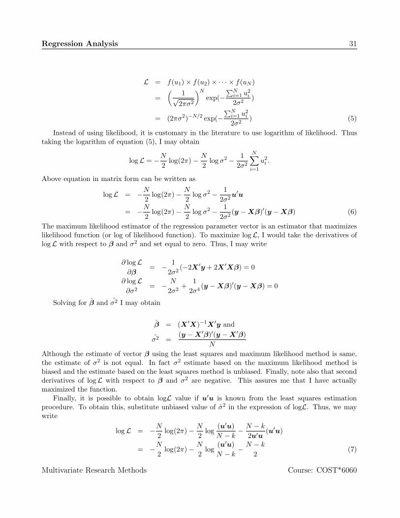
Instead of using likelihood, it is customary in the literature to use logarithm of likelihood. Thustaking the logarithm of equation (5), I may obtain
logL = −N
2log(2π) − N
2log σ2 − 1
2σ2
N∑
i=1
u2i .
Above equation in matrix form can be written as
logL = −N
2log(2π) − N
2log σ2 − 1
2σ2u′u
= −N
2log(2π) − N
2log σ2 − 1
2σ2(y − Xβ)′(y − Xβ) (6)
The maximum likelihood estimator of the regression parameter vector is an estimator that maximizeslikelihood function (or log of likelihood function). To maximize logL, I would take the derivatives oflogL with respect to β and σ2 and set equal to zero. Thus, I may write
∂ logL∂β
= − 12σ2
(−2X ′y + 2X ′Xβ) = 0
∂ logL∂σ2
= − N
2σ2+
12σ4
(y − Xβ)′(y − Xβ) = 0
Solving for β and σ2 I may obtain
β = (X ′X)−1X ′y and
σ2 =(y − X ′β)′(y − X ′β)
N
Although the estimate of vector β using the least squares and maximum likelihood method is same,the estimate of σ2 is not equal. In fact σ2 estimate based on the maximum likelihood method isbiased and the estimate based on the least squares method is unbiased. Finally, note also that secondderivatives of logL with respect to β and σ2 are negative. This assures me that I have actuallymaximized the function.
Finally, it is possible to obtain logL value if u′u is known from the least squares estimationprocedure. To obtain this, substitute unbiased value of σ2 in the expression of logL. Thus, we maywrite
logL = −N
2log(2π) − N
2log
(u′u)N − k
− N − k
2u′u(u′u)
= −N
2log(2π) − N
2log
(u′u)N − k
− N − k
2(7)
Multivariate Research Methods Course: COST*6060
Regression Analysis 32
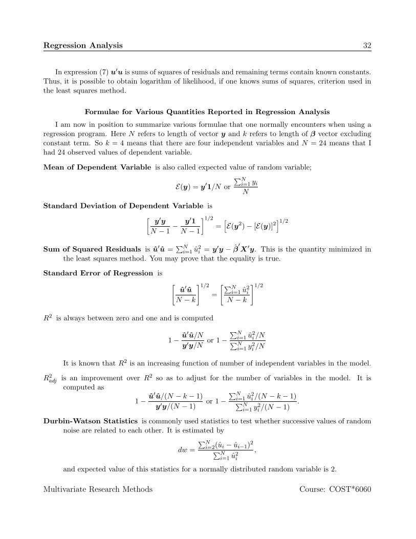
In expression (7) u′u is sums of squares of residuals and remaining terms contain known constants.Thus, it is possible to obtain logarithm of likelihood, if one knows sums of squares, criterion used inthe least squares method.
Formulae for Various Quantities Reported in Regression Analysis
I am now in position to summarize various formulae that one normally encounters when using aregression program. Here N refers to length of vector y and k refers to length of β vector excludingconstant term. So k = 4 means that there are four independent variables and N = 24 means that Ihad 24 observed values of dependent variable.
Mean of Dependent Variable is also called expected value of random variable;
E(y) = y′1/N or∑N
i=1 yi
N
Standard Deviation of Dependent Variable is[
y′y
N − 1− y′1
N − 1
]1/2
=[E(y2) − [E(y)]2
]1/2
Sum of Squared Residuals is u′u =∑N
i=1 u2i = y′y − β
′X ′y. This is the quantity minimized in
the least squares method. You may prove that the equality is true.
Standard Error of Regression is[
u′u
N − k
]1/2
=
[∑Ni=1 u2
i
N − k
]1/2
R2 is always between zero and one and is computed
1 − u′u/N
y′y/Nor 1 −
∑Ni=1 u2
i /N∑Ni=1 y2
i /N
It is known that R2 is an increasing function of number of independent variables in the model.
R2adj is an improvement over R2 so as to adjust for the number of variables in the model. It is
computed as
1 − u′u/(N − k − 1)y′y/(N − 1)
or 1 −∑N
i=1 u2i /(N − k − 1)
∑Ni=1 y2
i /(N − 1).
Durbin-Watson Statistics is commonly used statistics to test whether successive values of randomnoise are related to each other. It is estimated by
dw =∑N
i=2(ui − ui−1)2∑Ni=1 u2
i
,
and expected value of this statistics for a normally distributed random variable is 2.
Multivariate Research Methods Course: COST*6060
Regression Analysis 33
Estimated Autocorrelation or correlation among successive observation is
ρ =∑N
i=2 uiui−1/(N − 1)∑N
i=1 u2i /N
,
and expected value of this statistics for a normally distributed random variable is 0.
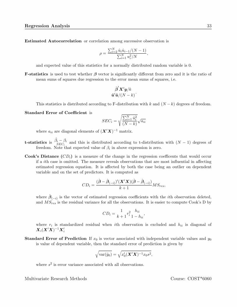
F-statistics is used to test whether β vector is significantly different from zero and it is the ratio ofmean sums of squares due regression to the error mean sums of squares, i.e.
β′X ′y/k
u′u/(N − k).
This statistics is distributed according to F-distribution with k and (N −k) degrees of freedom.
Standard Error of Coefficient is
SECi =
√∑Ni=1 u2
i
(N − k)√
aii
where aii are diagonal elements of (X ′X)−1 matrix.
t-statistics is βi − βiSECi
and this is distributed according to t-distribution with (N − 1) degrees offreedom. Note that expected value of βi in above expression is zero.
Cook’s Distance (CDi) is a measure of the change in the regression coefficents that would occurif a ith case is omitted. The measure reveals observations that are most influential in affectingestimated regression equation. It is affected by both the case being an outlier on dependentvariable and on the set of predictors. It is computed as
CDi =(β − β(−i))′(X
′X)(β − β(−i))k + 1
MSres,
where β(−i) is the vector of estimated regression coefficients with the ith observation deleted,and MSres is the residual variance for all the observations. It is easier to compute Cook’s D by
CDi =1
k + 1r2i
hii
1 − hii,
where ri is standardized residual when ith observation is excluded and hii is diagonal ofXi(X ′X)−1X ′
i
Standard Error of Prediction If x0 is vector associated with independent variable values and y0
is value of dependent variable, then the standard error of prediction is given by√
var(y0) =√
x′0(X
′X)−1x0s2,
where s2 is error variance associated with all observations.
Multivariate Research Methods Course: COST*6060
Regression Analysis 34
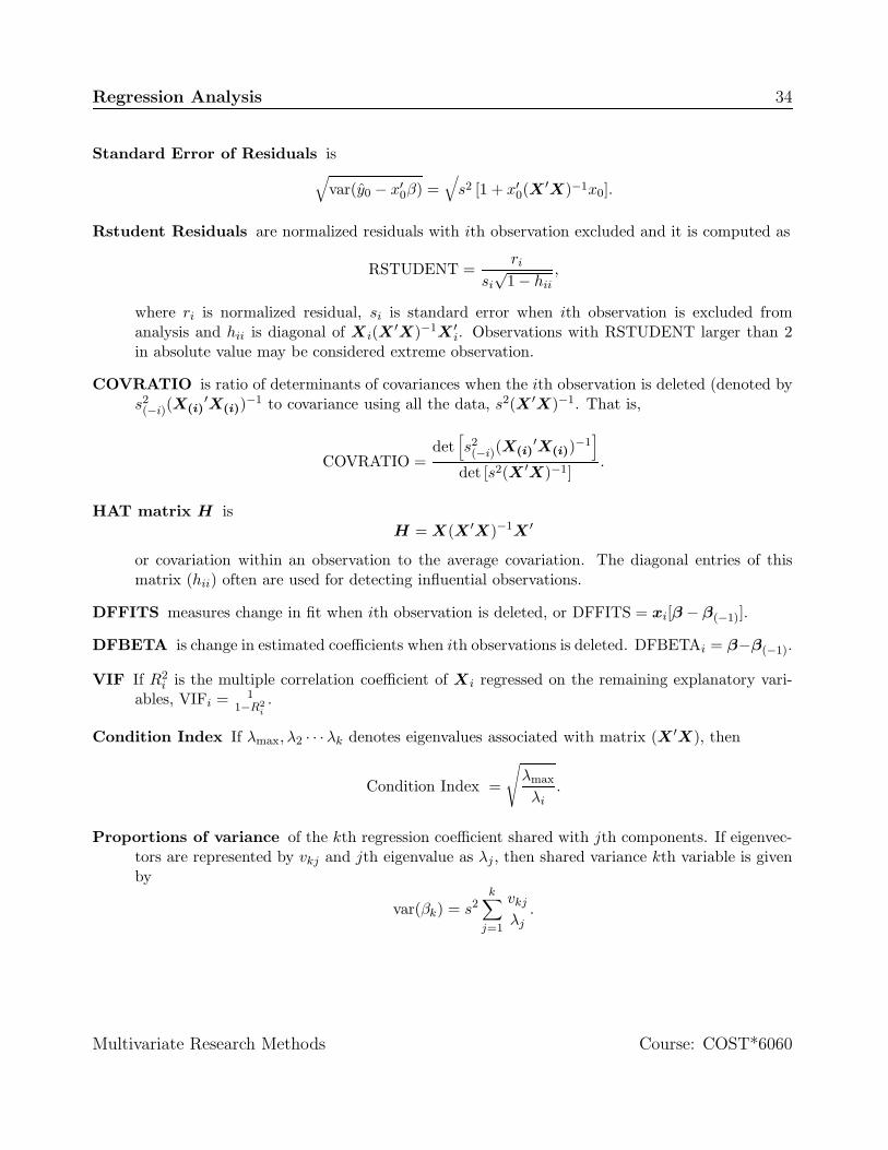
Standard Error of Residuals is√
var(y0 − x′0β) =
√s2 [1 + x′
0(X′X)−1x0].
Rstudent Residuals are normalized residuals with ith observation excluded and it is computed as
RSTUDENT =ri
si
√1 − hii
,
where ri is normalized residual, si is standard error when ith observation is excluded fromanalysis and hii is diagonal of Xi(X ′X)−1X ′
i. Observations with RSTUDENT larger than 2in absolute value may be considered extreme observation.
COVRATIO is ratio of determinants of covariances when the ith observation is deleted (denoted bys2(−i)(X(i)
′X(i))−1 to covariance using all the data, s2(X ′X)−1. That is,
COVRATIO =det
[s2(−i)(X(i)
′X(i))−1]
det [s2(X ′X)−1].
HAT matrix H isH = X(X ′X)−1X ′
or covariation within an observation to the average covariation. The diagonal entries of thismatrix (hii) often are used for detecting influential observations.
DFFITS measures change in fit when ith observation is deleted, or DFFITS = xi[β − β(−1)].
DFBETA is change in estimated coefficients when ith observations is deleted. DFBETAi = β−β(−1).
VIF If R2i is the multiple correlation coefficient of Xi regressed on the remaining explanatory vari-
ables, VIFi = 11−R2
i.
Condition Index If λmax, λ2 · · · λk denotes eigenvalues associated with matrix (X ′X), then
Condition Index =
√λmax
λi.
Proportions of variance of the kth regression coefficient shared with jth components. If eigenvec-tors are represented by vkj and jth eigenvalue as λj , then shared variance kth variable is givenby
var(βk) = s2k∑
j=1
vkj
λj.
Multivariate Research Methods Course: COST*6060
Related Documents