Recap from last time: live variables x := 5 y := x + 2 x := x + 1 y := x + 10 ... y ...

Recap from last time: live variables x := 5 y := x + 2 x := x + 1 y := x + 10... y...
Dec 21, 2015
Welcome message from author
This document is posted to help you gain knowledge. Please leave a comment to let me know what you think about it! Share it to your friends and learn new things together.
Transcript
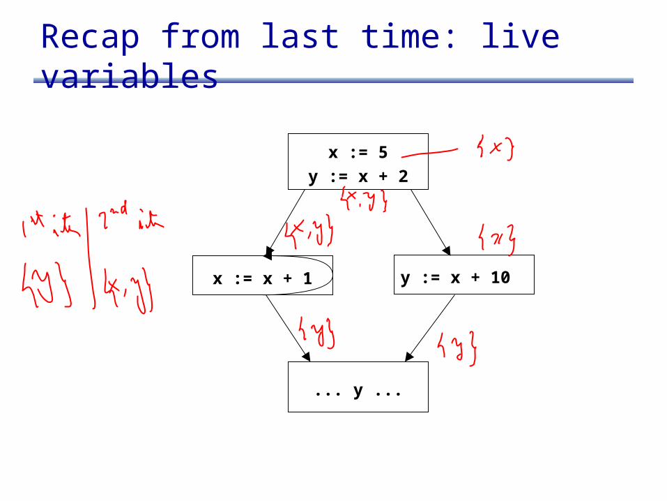
Recap from last time: live variables
x := 5
y := x + 2
x := x + 1 y := x + 10
... y ...
Revisiting assignment
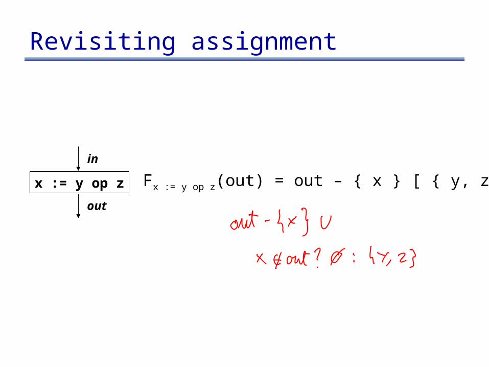
x := y op z
in
out
Fx := y op z(out) = out – { x } [ { y, z}
Theory of backward analyses
• Can formalize backward analyses in two ways
• Option 1: reverse flow graph, and then run forward problem
• Option 2: re-develop the theory, but in the backward direction
Precision
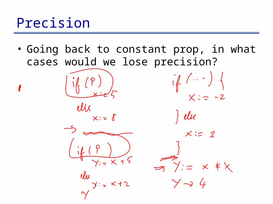
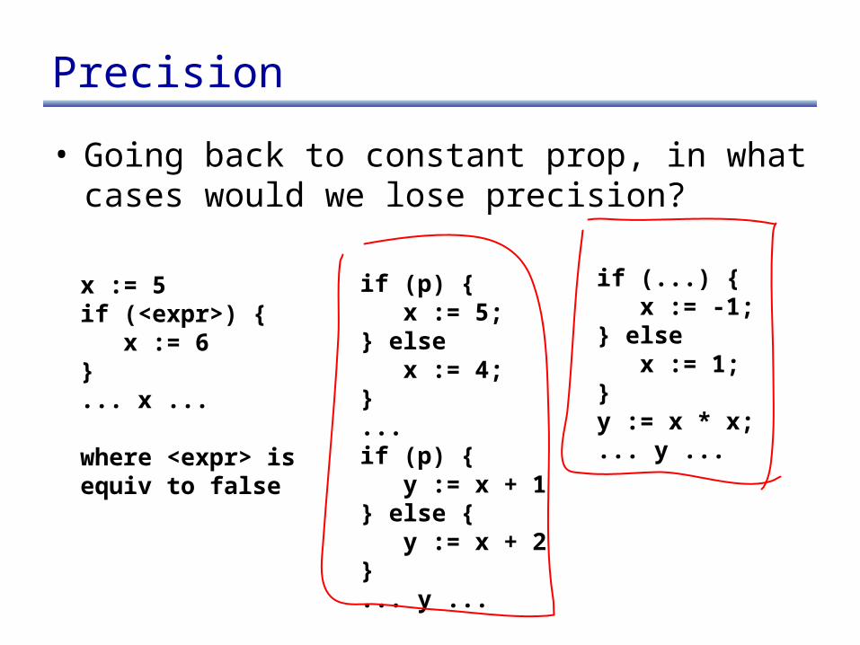
• Going back to constant prop, in what cases would we lose precision?
Precision
• Going back to constant prop, in what cases would we lose precision?
if (p) { x := 5;} else x := 4;}...if (p) { y := x + 1} else { y := x + 2}... y ...
if (...) { x := -1;} else x := 1;}y := x * x;... y ...
x := 5if (<expr>) { x := 6}... x ...
where <expr> is equiv to false
Precision
• The first problem: Unreachable code– solution: run unreachable code removal before– the unreachable code removal analysis will do its
best, but may not remove all unreachable code
• The other two problems are path-sensitivity issues– Branch correlations: some paths are infeasible– Path merging: can lead to loss of precision
MOP: meet over all paths
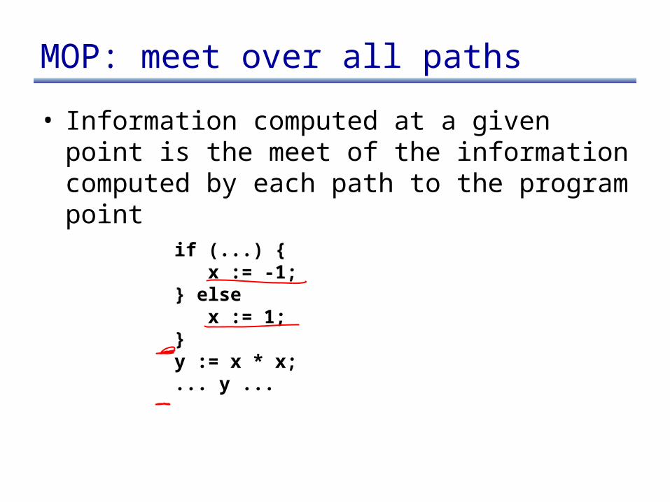
• Information computed at a given point is the meet of the information computed by each path to the program point
if (...) { x := -1;} else x := 1;}y := x * x;... y ...
MOP
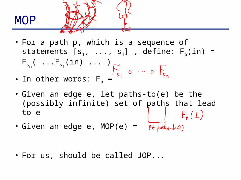
• For a path p, which is a sequence of statements [s1, ..., sn] , define: Fp(in) = Fsn
( ...Fs1(in) ... )
• In other words: Fp =
• Given an edge e, let paths-to(e) be the (possibly infinite) set of paths that lead to e
• Given an edge e, MOP(e) =
• For us, should be called JOP...
MOP vs. dataflow
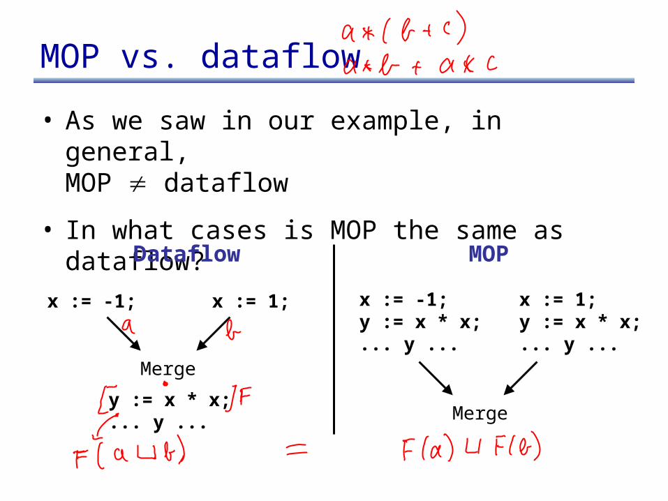
• As we saw in our example, in general,MOP dataflow
• In what cases is MOP the same as dataflow?
x := -1;y := x * x;... y ...
x := 1;y := x * x;... y ...
Merge
x := -1; x := 1;
Merge
y := x * x;... y ...
Dataflow MOP
MOP vs. dataflow
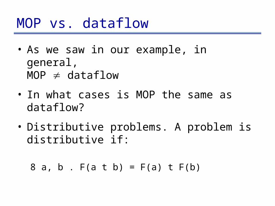
• As we saw in our example, in general,MOP dataflow
• In what cases is MOP the same as dataflow?
• Distributive problems. A problem is distributive if:
8 a, b . F(a t b) = F(a) t F(b)
Summary of precision
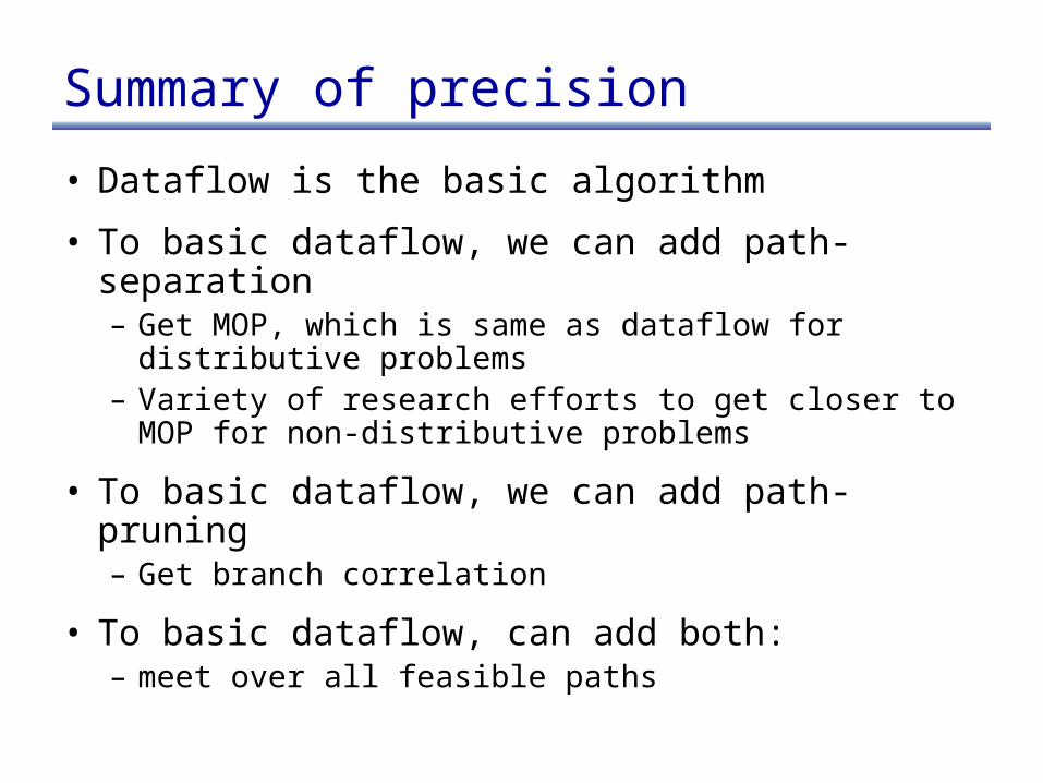
• Dataflow is the basic algorithm
• To basic dataflow, we can add path-separation– Get MOP, which is same as dataflow for distributive
problems– Variety of research efforts to get closer to MOP for
non-distributive problems
• To basic dataflow, we can add path-pruning– Get branch correlation
• To basic dataflow, can add both: – meet over all feasible paths

Program Representations

Representing programs
• Goals
Representing programs
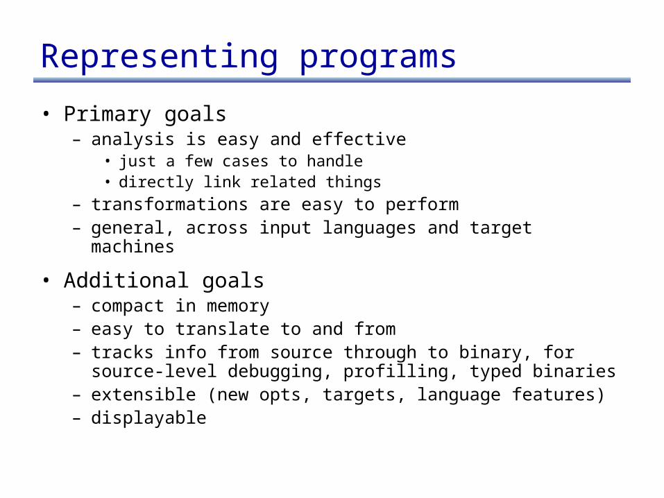
• Primary goals– analysis is easy and effective
• just a few cases to handle• directly link related things
– transformations are easy to perform– general, across input languages and target machines
• Additional goals– compact in memory– easy to translate to and from– tracks info from source through to binary, for source-level
debugging, profilling, typed binaries– extensible (new opts, targets, language features)– displayable
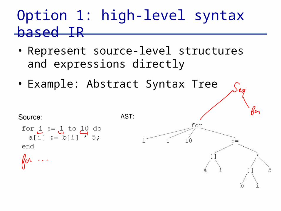
Option 1: high-level syntax based IR
• Represent source-level structures and expressions directly
• Example: Abstract Syntax Tree

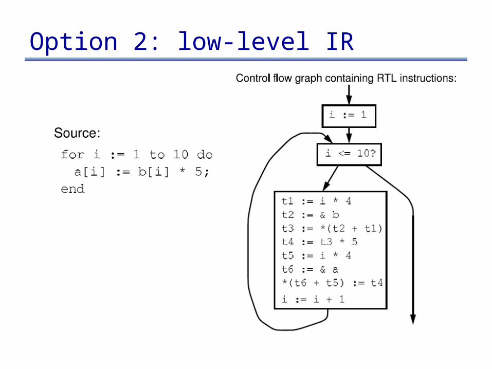
Option 2: low-level IR
• Translate input programs into low-level primitive chunks, often close to the target machine
• Examples: assembly code, virtual machine code (e.g. stack machines), three-address code, register-transfer language (RTL)
• Standard RTL instrs:
Option 2: low-level IR
Comparison
Comparison
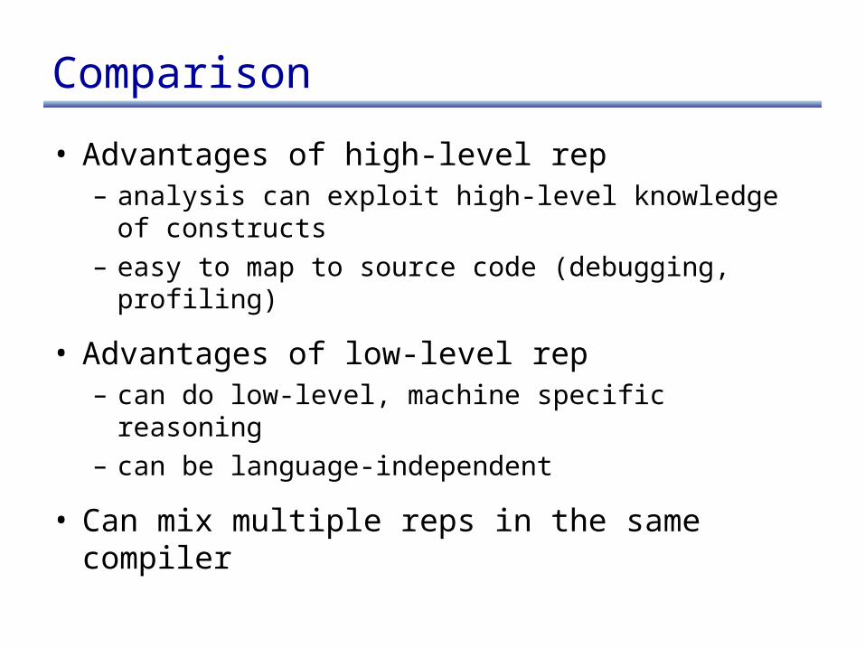
• Advantages of high-level rep– analysis can exploit high-level knowledge of
constructs– easy to map to source code (debugging, profiling)
• Advantages of low-level rep– can do low-level, machine specific reasoning– can be language-independent
• Can mix multiple reps in the same compiler
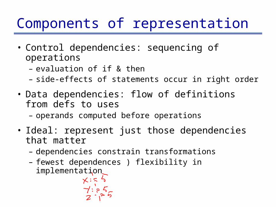
Components of representation
• Control dependencies: sequencing of operations– evaluation of if & then– side-effects of statements occur in right order
• Data dependencies: flow of definitions from defs to uses– operands computed before operations
• Ideal: represent just those dependencies that matter– dependencies constrain transformations– fewest dependences ) flexibility in implementation
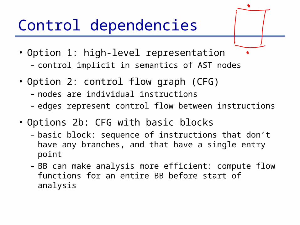
Control dependencies
• Option 1: high-level representation– control implicit in semantics of AST nodes
• Option 2: control flow graph (CFG)– nodes are individual instructions– edges represent control flow between instructions
• Options 2b: CFG with basic blocks– basic block: sequence of instructions that don’t have
any branches, and that have a single entry point– BB can make analysis more efficient: compute flow
functions for an entire BB before start of analysis
Control dependencies
• CFG does not capture loops very well
• Some fancier options include:– the Control Dependence Graph– the Program Dependence Graph
• More on this later. Let’s first look at data dependencies
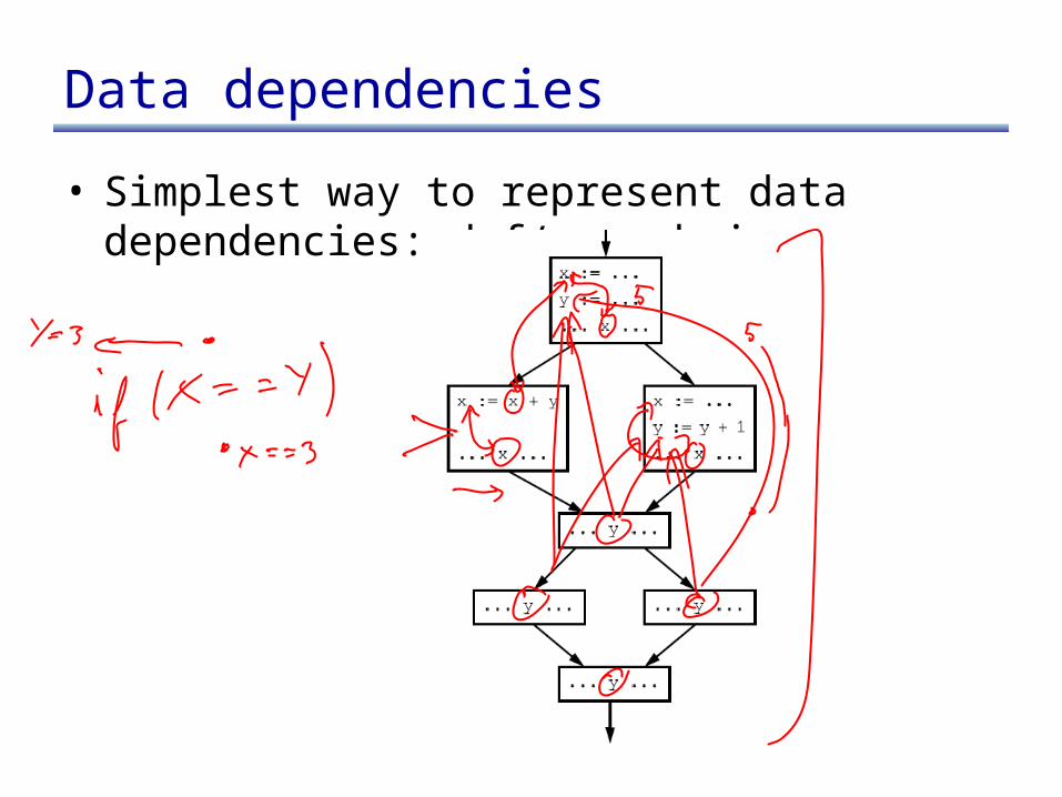
Data dependencies
• Simplest way to represent data dependencies: def/use chains
Def/use chains
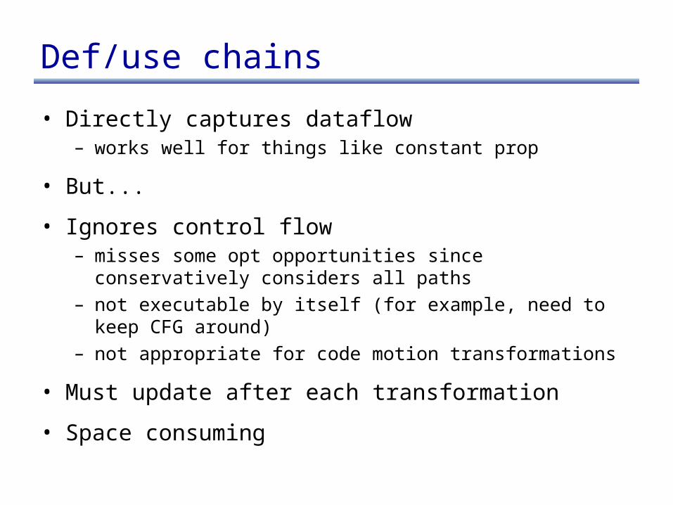
• Directly captures dataflow– works well for things like constant prop
• But...
• Ignores control flow– misses some opt opportunities since conservatively considers all
paths– not executable by itself (for example, need to keep CFG around)– not appropriate for code motion transformations
• Must update after each transformation
• Space consuming
SSA
• Static Single Assignment– invariant: each use of a variable has only one def
SSA
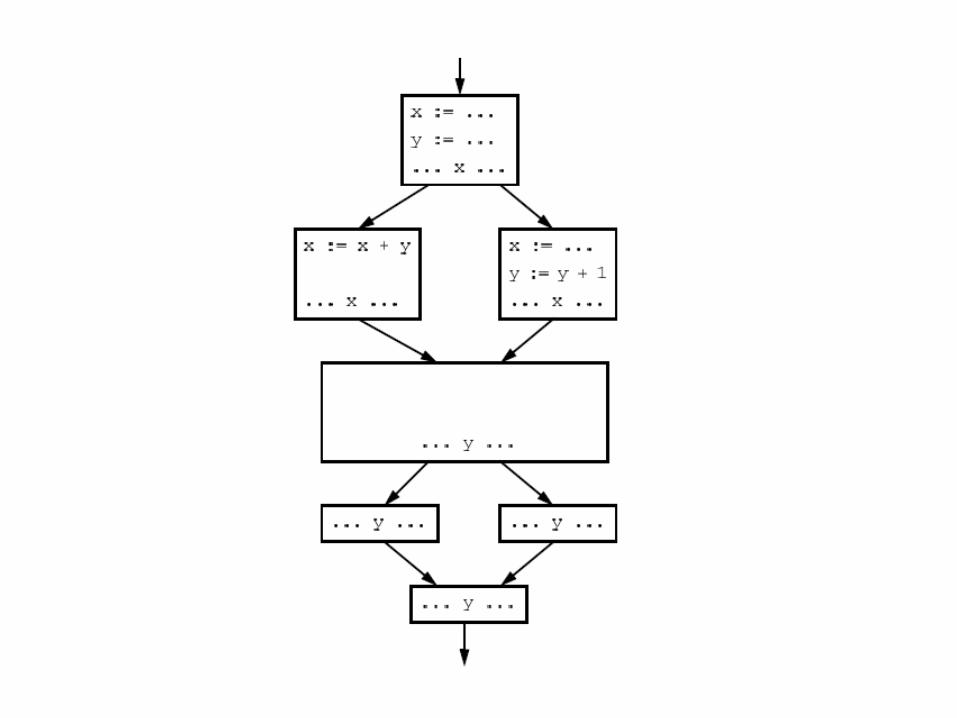
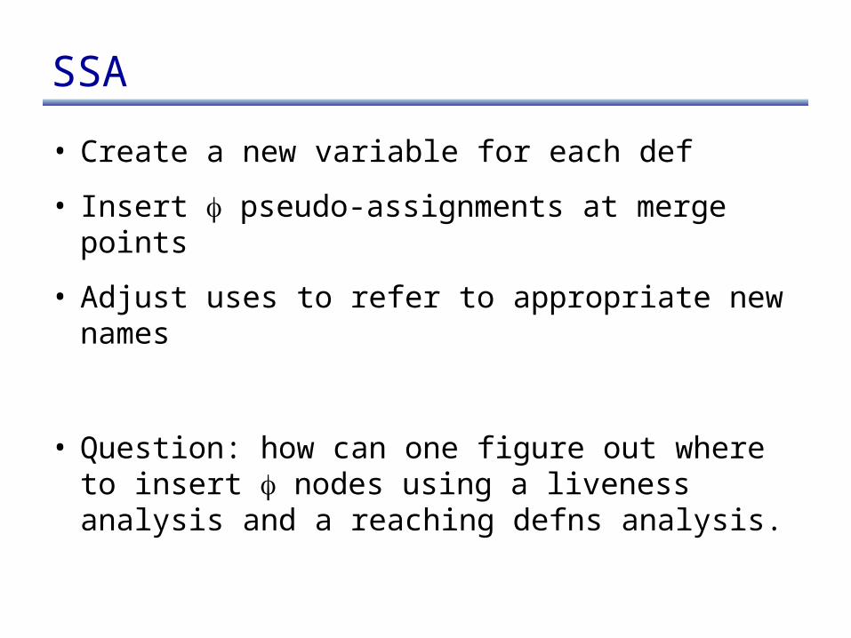
• Create a new variable for each def
• Insert pseudo-assignments at merge points
• Adjust uses to refer to appropriate new names
• Question: how can one figure out where to insert nodes using a liveness analysis and a reaching defns analysis.
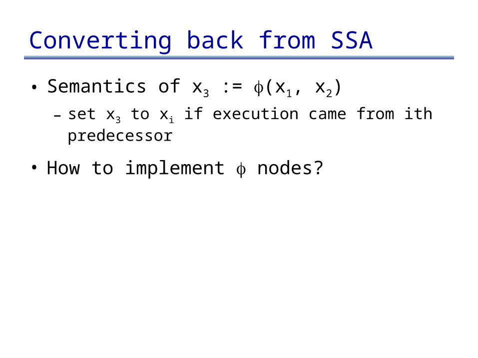
Converting back from SSA
• Semantics of x3 := (x1, x2)
– set x3 to xi if execution came from ith predecessor
• How to implement nodes?

Converting back from SSA
• Semantics of x3 := (x1, x2)
– set x3 to xi if execution came from ith predecessor
• How to implement nodes?– Insert assignment x3 := x1 along 1st predecessor
– Insert assignment x3 := x2 along 2nd predecessor
• If register allocator assigns x1, x2 and x3 to the same register, these moves can be removed– x1 .. xn usually have non-overlapping lifetimes, so this
is kind of register assignment is legal

Common Sub-expression Elim
• Want to compute when an expression is available in a var
• Domain:
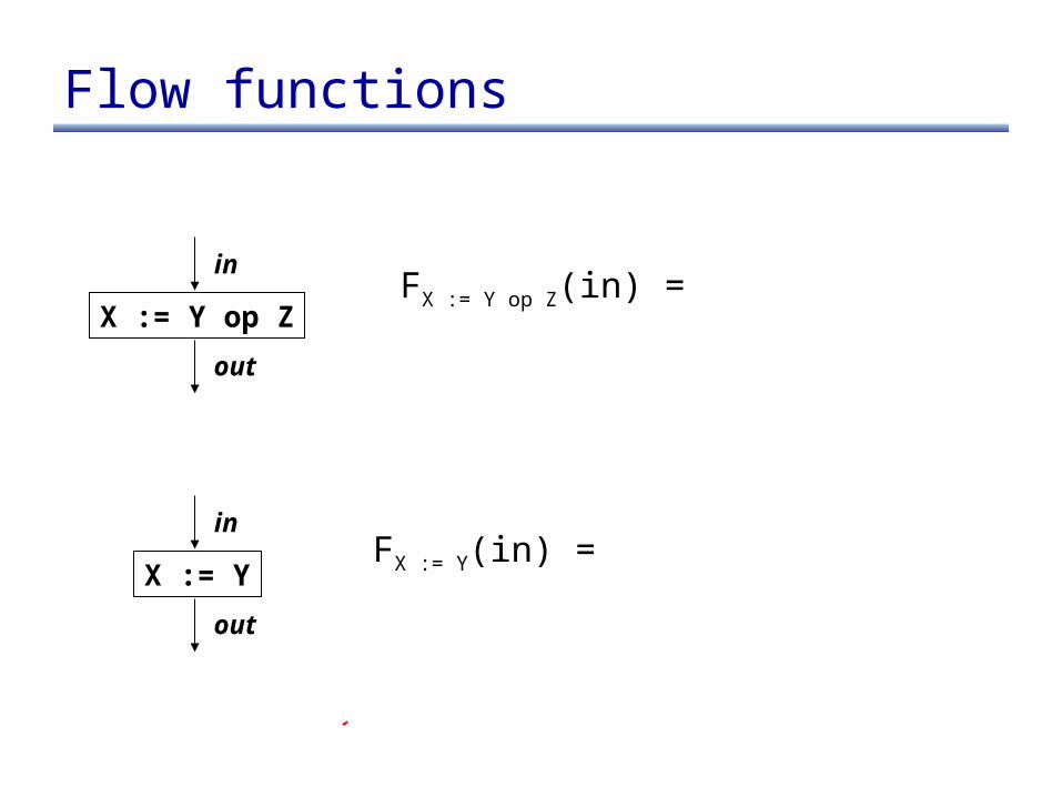
Flow functions
X := Y op Z
in
out
FX := Y op Z(in) =
X := Y
in
out
FX := Y(in) =
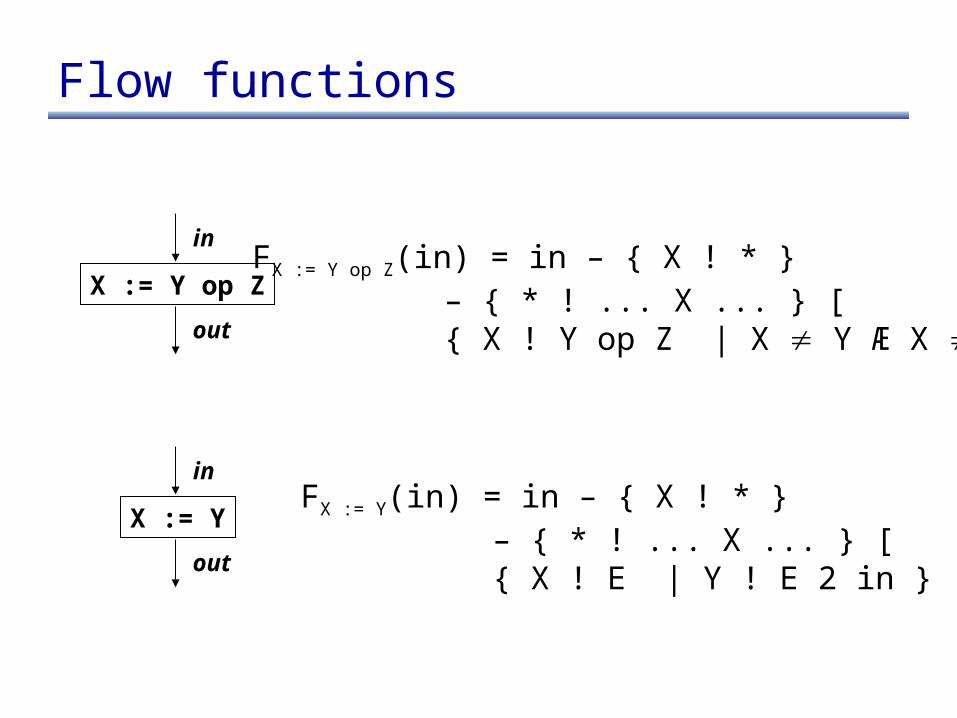
Flow functions
X := Y op Z
in
out
FX := Y op Z(in) = in – { X ! * } – { * ! ... X ... } [{ X ! Y op Z | X Y Æ X Z}
X := Y
in
out
FX := Y(in) = in – { X ! * } – { * ! ... X ... } [{ X ! E | Y ! E 2 in }
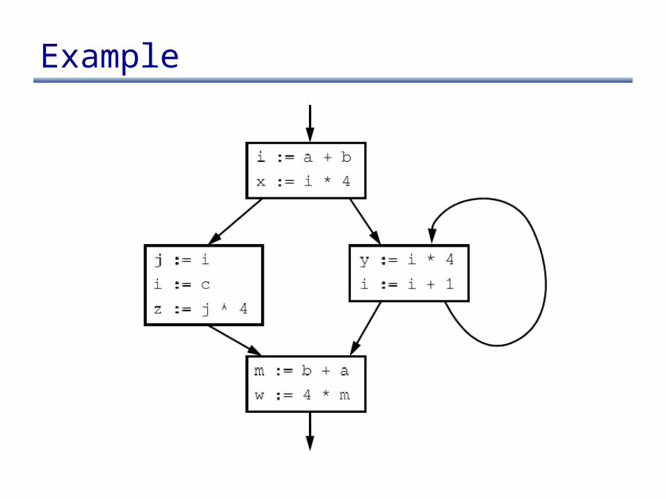
Example
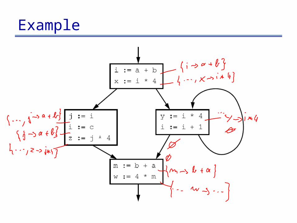
Example
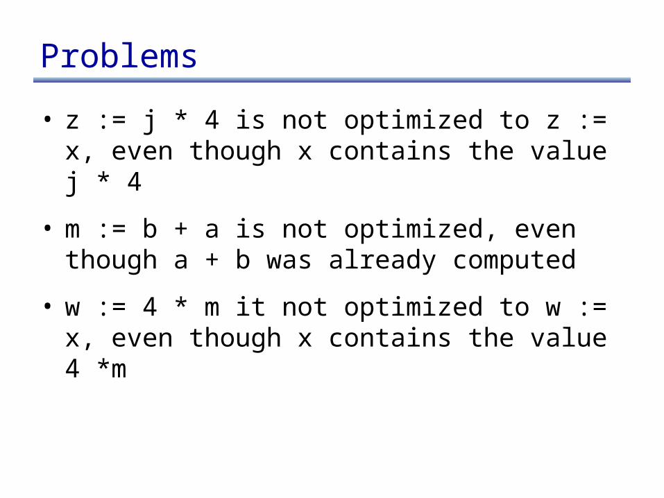
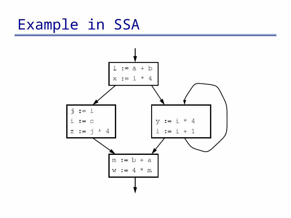
Problems
• z := j * 4 is not optimized to z := x, even though x contains the value j * 4
• m := b + a is not optimized, even though a + b was already computed
• w := 4 * m it not optimized to w := x, even though x contains the value 4 *m
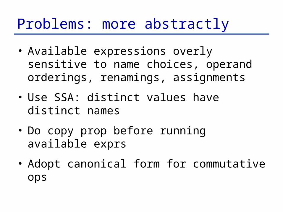
Problems: more abstractly
• Available expressions overly sensitive to name choices, operand orderings, renamings, assignments
• Use SSA: distinct values have distinct names
• Do copy prop before running available exprs
• Adopt canonical form for commutative ops
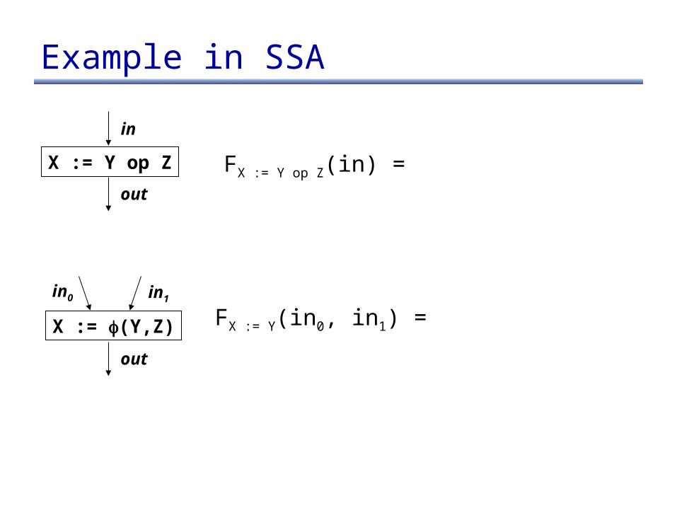
Example in SSA
X := Y op Z
in
out
FX := Y op Z(in) =
X := (Y,Z)
in0
out
FX := Y(in0, in1) =in1
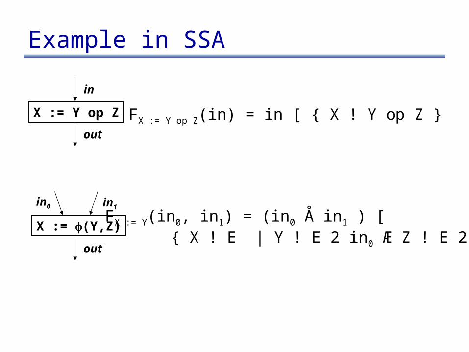
Example in SSA
X := Y op Z
in
out
FX := Y op Z(in) = in [ { X ! Y op Z }
X := (Y,Z)
in0
out
FX := Y(in0, in1) = (in0 Å in1 ) [ { X ! E | Y ! E 2 in0 Æ Z ! E 2 in1 }
in1
Example in SSA

Example in SSA
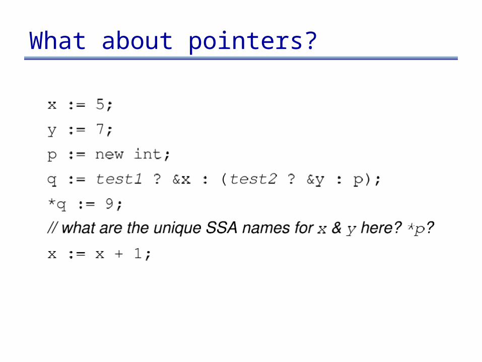
What about pointers?

What about pointers?
• Option 1: don’t use SSA for point-to memory
• Option 2: insert copies between SSA vars and real vars
SSA helps us with CSE
• Let’s see what else SSA can help us with
• Loop-invariant code motion
Loop-invariant code motion
• Two steps: analysis and transformations
• Step1: find invariant computations in loop– invariant: computes same result each time evaluated
• Step 2: move them outside loop– to top if used within loop: code hoisting– to bottom if used after loop: code sinking
Related Documents


