Real Time Control of Oscillations of Electric Power Systems · Real Time Control of Oscillations of Electric Power Systems ... 1 Normal vector and margin to the ... oscillations.

FINAL REPORT

ESEERCO PROJECT EP 95-11

Real Time Control of Oscillations of Electric Power Systems

September 1996

Prepared by:

Power Systems Engineering Research Consortium (PSerc)Cornell UniversityIthaca, NY 14853

Principal Investigators:

Pete Sauer, M. A. Pai, Stephen FernandesIan Dobson, Fernando Alvarado, Scott Greene

Bob Thomas, Hsiao-Dong Chiang

Prepared for:

Empire State Electric Energy Research Corporation1515 Broadway, 43rd Floor

New York, New York 10036-5701

and

New York State Electric & Gas

Copyright @ 1996EMPIRE STATE ELECTRICAL ENERGY RESEARCH CORPORATION

AND CORNELL UNIVERSITY.All Rights reserved

LEGAL NOTICE

This report was prepared as an account of work sponsored by the Empire State Electric Energy ResearchCorporation (�ESEERCO�) and New York State Electric and Gas Corporation (�NYSEG�). Neither ES-EERCO, members of ESEERCO, NYSEG nor any person acting on behalf of any of them:

a. Makes any warranty or representation, express or implied, with repsect to the accuracy, completeness,or usefulness of the information contained in this report, or that the use of any information, apparatus,method, or process disclosed in this report may not infringe on privately owned rights; or

b. Assumes any liability with respect to the use of, or for damages resulting from the use of, any infor-mation, apparatus, method, or process disclosed in this report.

Prepared by Cornell University, Ithaca, New York

ii

Acknowledgements

The authors gratefully acknowledge the interest and support of the Empire State Electric Energy ResearchCorp. and New York State Electric and Gas.

iii

Contents

1 Introduction 1

2 The Dynamic Model for Test Cases 2

3 Sensitivity of critical mode eigenvalues 4

4 Closeness to the Onset of Oscillation and its Sensitivity 7

4.1 Measuring the closeness to onset of oscillations with a marginM . . . . . . . . . . . . . . . 7

4.2 Computing the marginM with a continuation method . . . . . . . . . . . . . . . . . . . . . 8

4.3 The sensitivity ofM to parameters . . . . . . . . . . . . . . . . . . . . . . . . . . . . . . . 9

5 Single Machine Results 10

5.1 Test case system and data . . . . . . . . . . . . . . . . . . . . . . . . . . . . . . . . . . . . 10

5.2 Validation of margin sensitivity . . . . . . . . . . . . . . . . . . . . . . . . . . . . . . . . . 12

5.3 Validation of the control effectiveness . . . . . . . . . . . . . . . . . . . . . . . . . . . . . 13

6 37 Bus Equivalent Results 16

6.1 37 bus equivalent test case system and data . . . . . . . . . . . . . . . . . . . . . . . . . . 16

6.2 Eigenvalue analysis for load increase . . . . . . . . . . . . . . . . . . . . . . . . . . . . . . 16

6.3 Eigenvalue analysis - line outage . . . . . . . . . . . . . . . . . . . . . . . . . . . . . . . . 17

7 Computational Issues 18

8 Conclusions 18

A Appendix A 21

B Appendix B 22

iv

List of Figures

1 Normal vector and margin to the surface of critical parameter values . . . . . . . . . . . . . 8

2 Schematic of the single machine in"nite bus system test case . . . . . . . . . . . . . . . . . 11

3 Margin to Oscillatory Instability vs. Parameter . . . . . . . . . . . . . . . . . . . . . . . . . 13

v

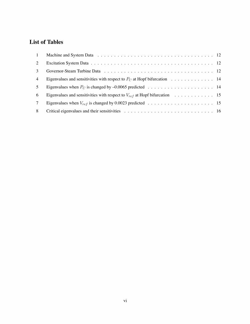
List of Tables

1 Machine and System Data . . . . . . . . . . . . . . . . . . . . . . . . . . . . . . . . . . . 12

2 Excitation System Data . . . . . . . . . . . . . . . . . . . . . . . . . . . . . . . . . . . . . 12

3 Governor-Steam Turbine Data . . . . . . . . . . . . . . . . . . . . . . . . . . . . . . . . . 12

4 Eigenvalues and sensitivities with respect to PC at Hopf bifurcation . . . . . . . . . . . . . 14

5 Eigenvalues when PC is changed by �0.0065 predicted . . . . . . . . . . . . . . . . . . . . 14

6 Eigenvalues and sensitivities with respect to Vref at Hopf bifurcation . . . . . . . . . . . . 15

7 Eigenvalues when Vref is changed by 0.0023 predicted . . . . . . . . . . . . . . . . . . . . 15

8 Critical eigenvalues and their sensitivities . . . . . . . . . . . . . . . . . . . . . . . . . . . 16

vi

Executive Summary

Contingencies or extreme system loading can cause unacceptable power system operating conditions suchas low voltages, excessive line #ows, or dynamic instabilities. The real-time controls needed to eliminatelow voltages or excessive line #ows are reasonably well understood either based on experience or apriorioperator guidelines. In contrast, real-time control strategies for dynamic instabilities are much less mature.Unbounded dynamic instabilities can cause rapid damage to equipment, usually providing insuf"cient timefor operator control. Automatic protective devices are assumed to provide the necessary real-time control.When dynamic instabilities are bounded, they appear as sustained oscillations or limit cycles which maynot cause protective devices to operate and therefore may require operator intervention to suppress them. Anumber of utilities have experienced these problems and heuristic methods to eliminate the oscillations havehad limited success.

This project investigated the feasibility of an approach to provide operator assistance in the predictionand suppresion of sustained system oscillations. The primary thrust of the project was based on a real-timesimulation which would track the system dynamic behavior. The monitor for the closeness of the systemto the onset of oscillations would be based on an indicator which provides a measure of the distance tooscillatory instability in terms of total load. The methods for suppressing sustained system oscillations wereto be based on eigenvalue sensitivity techniques which can provide a ranking of various control options.

Results on a single machine/in"nite bus system show that the concept is viable. Results on a 37 busequivalent system do not indicate feasibility for large-scale systems. The results indicate that eigenvaluemovement in response to typical operation controls can be suf"ciently nonlinear to make prediction ofremedial action unreliable. These and other computational issues are discussed in the following sections.

vii

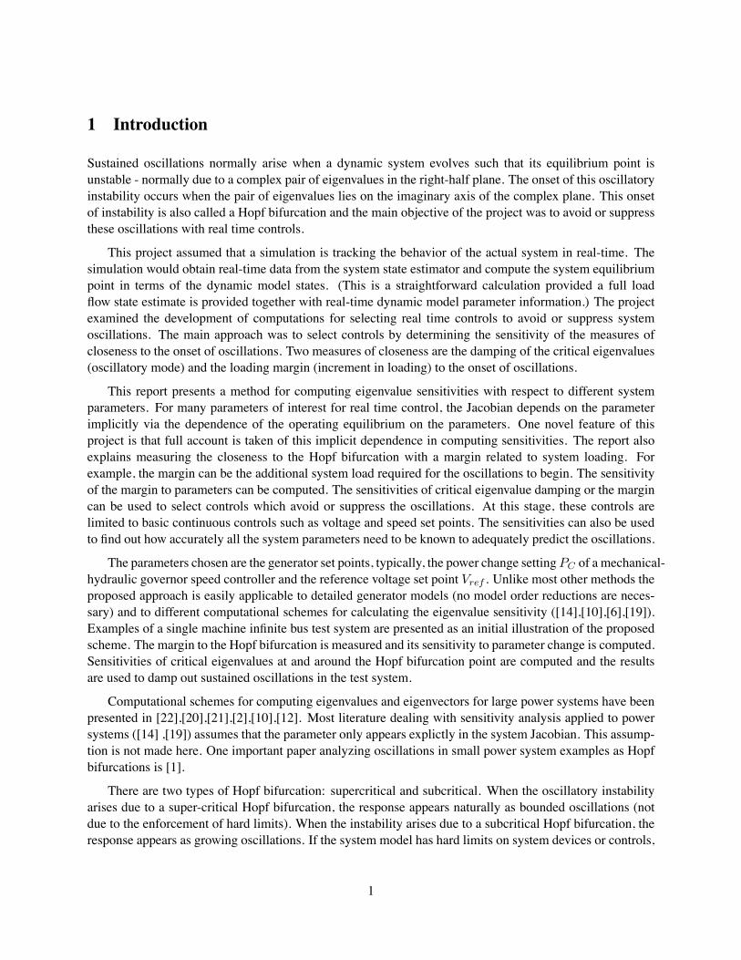
1 Introduction

Sustained oscillations normally arise when a dynamic system evolves such that its equilibrium point isunstable - normally due to a complex pair of eigenvalues in the right-half plane. The onset of this oscillatoryinstability occurs when the pair of eigenvalues lies on the imaginary axis of the complex plane. This onsetof instability is also called a Hopf bifurcation and the main objective of the project was to avoid or suppressthese oscillations with real time controls.

This project assumed that a simulation is tracking the behavior of the actual system in real-time. Thesimulation would obtain real-time data from the system state estimator and compute the system equilibriumpoint in terms of the dynamic model states. (This is a straightforward calculation provided a full load#ow state estimate is provided together with real-time dynamic model parameter information.) The projectexamined the development of computations for selecting real time controls to avoid or suppress systemoscillations. The main approach was to select controls by determining the sensitivity of the measures ofcloseness to the onset of oscillations. Two measures of closeness are the damping of the critical eigenvalues(oscillatory mode) and the loading margin (increment in loading) to the onset of oscillations.

This report presents a method for computing eigenvalue sensitivities with respect to different systemparameters. For many parameters of interest for real time control, the Jacobian depends on the parameterimplicitly via the dependence of the operating equilibrium on the parameters. One novel feature of thisproject is that full account is taken of this implicit dependence in computing sensitivities. The report alsoexplains measuring the closeness to the Hopf bifurcation with a margin related to system loading. Forexample, the margin can be the additional system load required for the oscillations to begin. The sensitivityof the margin to parameters can be computed. The sensitivities of critical eigenvalue damping or the margincan be used to select controls which avoid or suppress the oscillations. At this stage, these controls arelimited to basic continuous controls such as voltage and speed set points. The sensitivities can also be usedto "nd out how accurately all the system parameters need to be known to adequately predict the oscillations.

The parameters chosen are the generator set points, typically, the power change settingPC of a mechanical-hydraulic governor speed controller and the reference voltage set point Vref . Unlike most other methods theproposed approach is easily applicable to detailed generator models (no model order reductions are neces-sary) and to different computational schemes for calculating the eigenvalue sensitivity ([14],[10],[6],[19]).Examples of a single machine in"nite bus test system are presented as an initial illustration of the proposedscheme. The margin to the Hopf bifurcation is measured and its sensitivity to parameter change is computed.Sensitivities of critical eigenvalues at and around the Hopf bifurcation point are computed and the resultsare used to damp out sustained oscillations in the test system.

Computational schemes for computing eigenvalues and eigenvectors for large power systems have beenpresented in [22],[20],[21],[2],[10],[12]. Most literature dealing with sensitivity analysis applied to powersystems ([14] ,[19]) assumes that the parameter only appears explictly in the system Jacobian. This assump-tion is not made here. One important paper analyzing oscillations in small power system examples as Hopfbifurcations is [1].

There are two types of Hopf bifurcation: supercritical and subcritical. When the oscillatory instabilityarises due to a super-critical Hopf bifurcation, the response appears naturally as bounded oscillations (notdue to the enforcement of hard limits). When the instability arises due to a subcritical Hopf bifurcation, theresponse appears as growing oscillations. If the system model has hard limits on system devices or controls,

1

then these growing oscillations can be bounded as the limits prevent growth. Since this project is concernedwith the prediction and elimination of sustained oscillations, we are not seriously concerned about which ofthese two mechanism produces a given sustained oscillation.

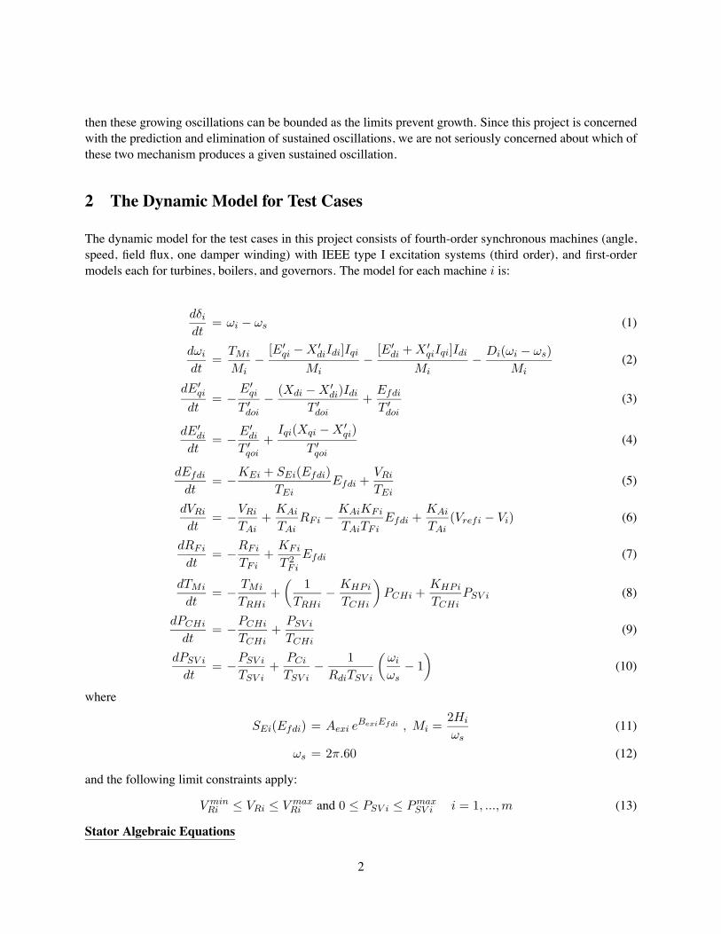
2 The Dynamic Model for Test Cases

The dynamic model for the test cases in this project consists of fourth-order synchronous machines (angle,speed, "eld #ux, one damper winding) with IEEE type I excitation systems (third order), and "rst-ordermodels each for turbines, boilers, and governors. The model for each machine i is:

dδidt

= ωi − ωs (1)

dωidt

=TMi

Mi−

[E′qi −X ′diIdi]IqiMi

−[E′di +X ′qiIqi]Idi

Mi− Di(ωi − ωs)

Mi(2)

dE′qidt

= −E′qiT ′doi

− (Xdi −X ′di)IdiT ′doi

+EfdiT ′doi

(3)

dE′didt

= −E′di

T ′qoi+Iqi(Xqi −X ′qi)

T ′qoi(4)

dEfdidt

= −KEi + SEi(Efdi)TEi

Efdi +VRiTEi

(5)

dVRidt

= −VRiTAi

+KAi

TAiRFi −

KAiKFi

TAiTFiEfdi +

KAi

TAi(Vrefi − Vi) (6)

dRFidt

= −RFiTFi

+KFi

T 2Fi

Efdi (7)

dTMi

dt= − TMi

TRHi+(

1TRHi

− KHPi

TCHi

)PCHi +

KHPi

TCHiPSV i (8)

dPCHidt

= −PCHiTCHi

+PSV iTCHi

(9)

dPSV idt

= −PSV iTSV i

+PCiTSV i

− 1RdiTSV i

(ωiωs− 1

)(10)

where

SEi(Efdi) = Aexi eBexiEfdi , Mi =

2Hi

ωs(11)

ωs = 2π.60 (12)

and the following limit constraints apply:

V minRi ≤ VRi ≤ V max

Ri and 0 ≤ PSV i ≤ PmaxSV i i = 1, ...,m (13)

Stator Algebraic Equations

2

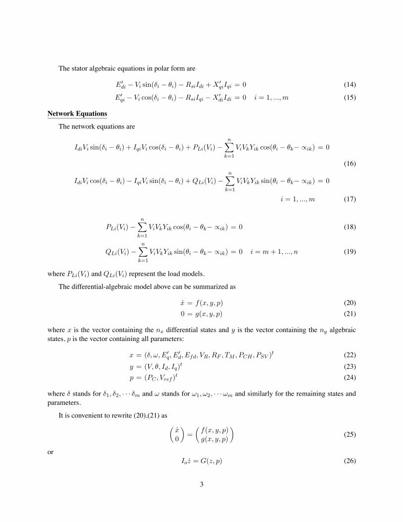
The stator algebraic equations in polar form are

E′di − Vi sin(δi − θi)−RsiIdi +X ′qiIqi = 0 (14)

E′qi − Vi cos(δi − θi)−RsiIqi −X ′diIdi = 0 i = 1, ...,m (15)

Network Equations

The network equations are

IdiVi sin(δi − θi) + IqiVi cos(δi − θi) + PLi(Vi)−n∑k=1

ViVkYik cos(θi − θk− ∝ik) = 0

(16)

IdiVi cos(δi − θi)− IqiVi sin(δi − θi) +QLi(Vi)−n∑k=1

ViVkYik sin(θi − θk− ∝ik) = 0

i = 1, ...,m (17)

PLi(Vi)−n∑k=1

ViVkYik cos(θi − θk− ∝ik) = 0 (18)

QLi(Vi)−n∑k=1

ViVkYik sin(θi − θk− ∝ik) = 0 i = m+ 1, ..., n (19)

where PLi(Vi) and QLi(Vi) represent the load models.

The differential-algebraic model above can be summarized as

x = f(x, y, p) (20)

0 = g(x, y, p) (21)

where x is the vector containing the nx differential states and y is the vector containing the ny algebraicstates, p is the vector containing all parameters:

x = (δ, ω,E′q, E′d, Efd, VR, RF , TM , PCH , PSV )t (22)

y = (V, θ, Id, Iq)t (23)

p = (PC , Vref )t (24)

where δ stands for δ1, δ2, · · · δm and ω stands for ω1, ω2, · · ·ωm and similarly for the remaining states andparameters.

It is convenient to rewrite (20),(21) as (x0

)=(f(x, y, p)g(x, y, p)

)(25)

orIoz = G(z, p) (26)

3

where

z =(xy

)(27)

Io =(Inx×nx Onx×nyOny×nx Ony×ny

)(28)

G(z, p) =(f(x, y, p)g(x, y, p)

)(29)

3 Sensitivity of critical mode eigenvalues

The background and formulas for the eigenvalue sensitivity are now presented. Discussion of technicalmathematical assumptions is postponed to the end of the section. The derivation combines together ap-proaches from ([6],[15],[10] ,[19])

Differential equations can be obtained from the differential algebraic model (20) and (21) by eliminatingthe algebraic states y. Solving the algebraic equations (21) for y in terms of x yields a function

y = h(x, p) (30)

Substitution of h(x, p) for y in (20) yields the differential equations

x = f(x, h(x, p), p) (31)

= F (x, p) (32)

Supercripts are used to indicate the ith component of a vector. For example the ith component of the vectorx is xi and the ith equation of (32) is

xi = F i(x, p) (33)

Since h was derived by solving the algebraic equations (21),

0 = g(x, h(x, p), p) (34)

The Jacobian hx of h with respect to x is obtained by differentiating (34):

0 = gx + gyhx (35)

hx = −g−1y gx (36)

Now the system Jacobian Fx can be expressed in terms of f and g by differentiating (32):

Fx = fx + fyhx = fx − fyg−1y gx (37)

The system eigenvalues are the eigenvalues of the Jacobian matrix Fx. Let λ be one of these eigenvaluesand let v and w be the right and left eigenvectors associated with λ. w is a row vector and v is a columnvector.

Write

v =(

vhxv

)=(

v−g−1

y gxv

)(38)

4

Then, using (37)

Gz v =(fx fygx gy

)(v

−g−1y gxv

)=(

(fx − fyg−1y gx)v

0

)=(Fxv

0

)= λ

(v0

)= λIov (39)

Similarly, writew = (w, −wfyg−1

y ) (40)

and obtain

wGz = (w, −wfyg−1y )

(fx fygx gy

)= (w(fx − fyg−1

y gx), 0 ) = (wFx, 0 ) = λ (w, 0 ) = λwIo

(41)The vector v de"nes the mode shape of both the differential and algebraic variables in the same way as theeigenvector v de"nes the mode shape of the differential variables. (The equation Gz v = λIov is called ageneralized eigenvalue problem [8], [19].)

The operating point or equilibrium of (26) is written as Z(p) and satis"es

0 = G(Z(p), p) (42)

The equilibrium Z(p) is a function of the parameter p. The sensitivity of this equilibrium with respect to pis the vector Zp = ∂Z

∂p which can be evaluated by differentiating (42) and rearranging terms:

0 = GzZp +Gp (43)

Zp = −(Gz)−1Gp (44)

The ith components of equations (43) and (44) can be written as

0 =∑j

∂Gi

∂zjZjp +

∂Gi

∂p(45)

Zip = −∑j

[(Gz)−1

]ij ∂Gj∂p

(46)

For practical computation of Zp, explicit evaluation of the inverse (Gz)−1 is avoided and sparse methodsare used.

In the differential-algebraic equations (26), G is a function of z and p. Therefore the Jacobian of thedifferential-algebraic equationsGz(z, p) is also a function of z and p. When the Jacobian of the differential-algebraic equations is evaluated at the equilibrium Z(p), it can be regarded as function J(p) of p:

J(p) = Gz(Z(p), p) (47)

That is, J varies with the parameter p, not only because the entries of the Jacobian might depend directly onp but also because the equilibrium position Z(p) might vary with p and the Jacobian is evaluated at Z(p).

Evaluating (39) and (41) at (Z(p), p) gives

Jv = λIov (48)

wJ = λwIo (49)

5

and hence0 = w(J − λIo)v (50)

To obtain the eigenvalue sensitivity, differentiate (50) with respect to p to obtain

0 = w(Jp − λpIo)v (51)

(The other terms involving vp and wp vanish). Rearrangement of (51) and using wIov = wv gives a formulafor the eigenvalue sensitivity λp = ∂λ

∂p with respect to the parameter p:

λp =wJpv

wv=

∑i,j

wiJ ijp vj

∑i

wivi(52)

It remains to express J ijp in terms of derivatives of G. The i, j component of equation (47) is

J ij(p) = Gijz (Z(p), p) =∂Gi

∂zj(Z(p), p) (53)

Differentiate (53) with respect to p to obtain

J ijp =∑k

∂2Gi

∂zj∂zkZkp +

∂2Gi

∂zj∂p(54)

and substitute in (52) to "nally obtain the eigenvalue sensitivity formula

λp =

∑i,j,k

wi∂2Gi

∂zj∂zkZkp v

j +∑i,j

wi∂2Gi

∂zj∂pvj

∑i

wivi(55)

The "rst term in (55) describes "rst order changes in the eigenvalue λ due to changes in p affecting theequilibrium position at which the Jacobian is evaluated and the second term describes "rst order changes inλ due to changes in p affecting the entries of the Jacobian directly.

There are some technical assumptions required to make the procedure above rigorous:

• The limits (13) are neglected to ensure that f and g are smooth functions.

• The construction of the function h in (30) requires gy to be assumed invertible. According to theimplicit function theorem, h is well de"ned locally if gy is invertible. The construction of w and valso requires gy to be invertible.

• The eigenvalue λ is assumed to be unique and simple. The simplicity of λ ensures that wv 6= 0 so thatthe division by wv in (55) is valid. The uniqueness of λ ensures that w and v are unique up to scalingby a constant.

• The computation of Zp requires that Gz is invertible (see (44)).

6

4 Closeness to the Onset of Oscillation and its Sensitivity

This section explains how to compute the closeness or margin to onset of oscillation and the sensitivity ofthis margin to parameters.

4.1 Measuring the closeness to onset of oscillations with a marginM

The closeness to the onset of oscillation is measured by the change in one of the parameters required forthe system to be at the onset of oscillation. Suppose the change in parameter isM (M stands for Marginto onset of oscillation). The choice of which parameter is used for M must be made according to whichparameter is most meaningful as a measure of closeness. For example, in the single machine in"nite busexample, the parameter PC describes (in some sense) the system loading and the change in PC could bea good choice for M . In this case, M = PC would describe the increase in loading before the onset ofoscillations. In a multibus system with several areas, it might be appropriate to chooseM as the change ina critical interarea #ow. In this case,M would describe an increase in this interarea #ow which would leadto the onset of oscillations. Alternatively, system loading in a multibus system could be used as a marginby picking a speci"c pattern of load increase and then de"ningM to be the amount of load increase in thatspeci"c pattern.

To explain and de"ne the margin M more precisely, supose that the power system has an equilibriumwhen the parameters are p0. Suppose "rst that M is chosen to re#ect changes in the "rst parameter in thevector p. De"ne the unit vector

k =

10...0

(56)

(a more general choice of k is used below) and consider p changing from p0 according to

p = p0 +mk (57)

as the scalar m increases from zero. Suppose that as m increases, the "rst onset of instability occurs at p∗.ThenM is de"ned so that

p∗ = p0 +Mk (58)

That is,M = kT (p∗ − p0) (59)

Thus when k is given by (56),M measures the change of the "rst parameter from its value at p0 to its valueat the onset of oscillations at p∗.

It is now straightforward to allow a more general choice of the unit vector k to allow for the individualor joint variation of other parameters when de"ningM . If (56) is replaced by a more general choice of k,then equations (57,58,59) immediately apply and now M measures the change of the parameter p in thedirection k from its value at p0 to its value at the onset of oscillations at p∗. This is illustrated in the case ofthe vector p containing two parameters in Figure 1

In the case of a power system with many loads which are represented by their real and reactive powerdemands appearing as parameters in the model, k could be thought of as de"ning the pattern or direction

7

Se

cond

Pa

ram

ete

r

First Parameter

M

k

N

p0

p*

Figure 1: Normal vector and margin to the surface of critical parameter values

of load increase. In this case M measures the margin to the onset of oscillations as loads increase in theproportions indicated by the entries of k.

The marginM can be useful either when the system is stable or unstable when the parameters are p0. Ifp0 corresponds to a stable operating equilibrium, thenM is the margin to p0 becoming oscillatory unstableat p∗. In this case one would usually set up the de"nition ofM so that theM is positive. If p0 is oscillatoryunstable, then the power system cannot operate at p0. (However, it is quite likely that the power system isoscillating around p0.) However, the closeness of the parameters p0 to parameters p∗ at which the oscillatoryinstability of the equilibrium is "rst suppressed can be measured with a marginM . It is possible to set upthe de"nition ofM so thatM would be negative in this case. Thus the marginM can be used to measure the�distance to the onset of oscillations in parameter space� when the equilibrium is either stable or unstable.

4.2 Computing the marginM with a continuation method

The main idea of a continuation method is to repeatedly calculate equilibrium solutions as the parametervaries in small steps. The parameter variation is determined by the direction of parameter variation k andthe step size ∆m. The parameter variation continues until the onset of oscillations is reached. The value ofthe parameter at the onset of oscillations then determines the marginM .

That is, the continuation begins by computing the equilibrium Z(p0) and then computes Z(p0 + ∆mk),

8

Z(p0 + 2∆mk), Z(p0 + 3∆mk), · · ·. Each equilibrium is checked for oscillatory instability and the con-tinuation ends when the onset of oscillations has been reached. For example, if Z(p0 + (i − 1)∆mk) is astable equilibrium and Z(p0 + i∆mk) is oscillatory unstable, then the onset of oscillations occurs betweenp0 + (i− 1)∆mk and p0 + i∆mk and the marginM must satisfy (i− 1)∆m ≤M ≤ i∆m. The estimateofM can then be re"ned by locating the onset of oscillations more exactly.

There are three numerical tasks to be addressed when computingM using continuation:

1. Ef"ciently compute the successive equilibria as the parameter is incremented.

2. Detect the onset of oscillations between steps

3. Locate the onset of oscillations to the desired accuracy

There is an extensive body of numerical analysis which addresses these tasks; a good general reference is[18].

4.3 The sensitivity ofM to parameters

Suppose that the power system is operating at a stable equilibrium corresponding to the vector of parametersp0 and that the marginM to the onset of oscillations at p∗ has been determined. The objective is to changesome of the parameters in p0 to increase M in order to improve the system security. Then it is useful tocompute the sensitivityMp0 of the marginM to variation of the parameters p0 [6]. Mp0 is a vector whoseith component is the sensitivity ofM with respect to the ith parameter in the vector p0. Mp0 quanti"es to"rst order the effect onM of changing each parameter in p0 and knowledge ofMp0 allows the most effectiveparameters to be selected. (Mp0 is also useful if the power system has an unstable equilibrium correspondingto p0 and the objective is to choose parameter changes to stabilize the unstable equilibrium.)

The sensitivityMp0 can be easily computed from eigenvalue sensitivities λp evaluated at p∗. (Formulasfor λp are given in (55)). De"ne the vector

N = Re{λp(p∗)} (60)

(Re means real part.) Then it can be shown [6, 5] thatMp0 is simply a scaled version of N :

Mp0 =−NNk

=−N∑

j

N jkj(61)

Thus the margin sensitivityMp0 is very easy to compute from eigenvalue sensitivities at the onset of oscil-lations p∗.

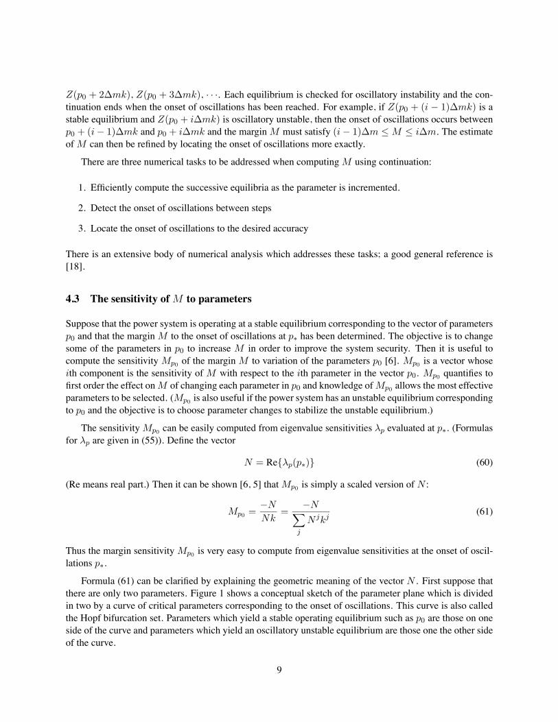
Formula (61) can be clari"ed by explaining the geometric meaning of the vector N . First suppose thatthere are only two parameters. Figure 1 shows a conceptual sketch of the parameter plane which is dividedin two by a curve of critical parameters corresponding to the onset of oscillations. This curve is also calledthe Hopf bifurcation set. Parameters which yield a stable operating equilibrium such as p0 are those on oneside of the curve and parameters which yield an oscillatory unstable equilibrium are those one the other sideof the curve.

9

Since parameter values on the curve correspond to the onset of oscillations, the real part of a particularsystem eigenvalue λ must vanish. Indeed, this property de"nes an equation for the curve:

0 = Re{λ(p)} (62)

The normal vector to the curve is obtained by differentiating (62) with respect to p:

normal vector at p∗ =d

dpRe{λ(p)}(p∗) = Re{λp(p∗)} = N (63)

ThusN is a vector normal to the critical curve of parameters. Equation (63) relates the eigenvalue sensitivityλp(p∗) to the geometry of the curve. A normal vector to the curve de"nes an ef"cient direction to changeparameters to move away from the curve and this fact underlies the appearance of N in (61).

In practical power systems there are many parameters so that the parameter space is multidimensional.Now the critical set of parameters which correspond to the onset of oscillations is a hypersurface (a sur-face of dimension one less than the number of parameters; for example, if there are two parameters, thehypersurface is the one dimensional curve of Figure 1; if there are three parameters, the hypersurface is atwo dimensional surface; if there are 100 parameters, the hypersurface is a 99 dimensional surface). Theequations above and the interpretation of N as a normal vector to the hypersurface remain valid. Indeed, itis in the multidimensional case of many parameters that the computations are most useful in assisting theengineering choice of which parameters are best to increase the margin.

5 Single Machine Results

This section presents results for a single machine/in"nite bus test system. The results show that the conceptis viable for this case.

5.1 Test case system and data

The test case system used in Task 1 is a single machine in"nite bus system as shown in Figure 2 with thedata of Tables 1-3.

10

+_

+

_

+_[(X -X )I +jE ]ed qq q

j( d - p/2) V Ð0¥(V+jV )ed

j( d - p/2)q

(I + jI )eqdj( d - p/2) jXeR s Re

jXd¢

¢ ¢

Figure 2: Schematic of the single machine in"nite bus system test case

For the test case, the network equations can be simpli"ed to:

ReId −XeIq − V sin(δ − θ) + V∞ sin δ = 0 (64)

XeId +ReIq − V cos(δ − θ) + V∞ cos δ = 0 (65)

11

The Single Machine In"nite Bus Test Case Data

Table 1: Machine and System Data

Rs Xd Xq X ′d X ′q0.00185 p.u. 1.942 p.u. 1.921 p.u. 0.330 p.u. 0.507 p.u.

T ′do T ′qo H D Re+ jXe

5.330 sec 0.593 sec 2.8323 sec 0.0 p.u. 0.001+j0.5 p.u.

Table 2: Excitation System Data

KA TA KE TE KF

50 p.u. 0.02 sec. 1.0 p.u. 0.78 sec. 0.01 p.u.

TF Aex Bex Vmax Vrmin1.2 sec. 0.397 p.u. 0.09 p.u. 9.9 p.u. -8.9 p.u.

Table 3: Governor-Steam Turbine Data

TRH KHP TCH TSV Rd10.0 sec. 0.26 p.u. 0.5 sec. 0.2 sec. 0.05 p.u.

5.2 Validation of margin sensitivity

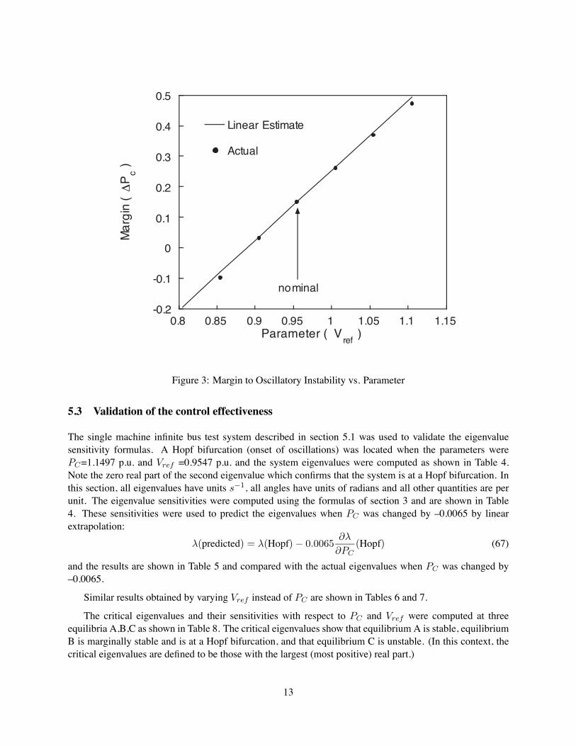
The single machine example has only two parameters PC and Vref . (These parameters are measured in perunit.) The power system has a stable equilibrium when PC = 1.0 and Vref = 0.9547 and these values areplotted as a point labelled �nominal� in Figure 3.

PC is varied from 1.0 until the onset of oscillations occurs at PC∗ = 1.1497 (Vref is held constant at0.9547). The marginM to the onset of oscillations is measured with the change in PC :

M = PC∗ − 1.0 (66)

(In the more general notation of section 4.1, p0 = (1.0, 0.9547)t, p∗ = (PC∗, 0.9547)t, k = (1, 0)t.) Forthe nominal values of PC = 1.0 and Vref = 0.9547, (PC∗ is computed to be 1.1497 and hence the marginisM = 0.1497.

The sensitivity in the marginM with respect to Vref was computed using formulas (33). This sensitivitywas used to plot the straight line through the nominal point in Figure 3. Thus the margin sensitivity formulasgive a linear approximation to the changes in M resulting from changes in Vref at the stable equilibrium.The computed margin sensitivity was validated by computing the exact margin for several values of Vref ;these are plotted as large dots in Figure 3.

12

-0.2

-0.1

0

0.1

0.2

0.3

0.4

0.5

0.8 0.85 0.9 0.95 1 1.05 1.1 1.15

Linear Estimate

Actual

Ma

rgin

( D

Pc )

Parameter ( Vref

)

nominal

Figure 3: Margin to Oscillatory Instability vs. Parameter

5.3 Validation of the control effectiveness

The single machine in"nite bus test system described in section 5.1 was used to validate the eigenvaluesensitivity formulas. A Hopf bifurcation (onset of oscillations) was located when the parameters werePC=1.1497 p.u. and Vref =0.9547 p.u. and the system eigenvalues were computed as shown in Table 4.Note the zero real part of the second eigenvalue which con"rms that the system is at a Hopf bifurcation. Inthis section, all eigenvalues have units s−1, all angles have units of radians and all other quantities are perunit. The eigenvalue sensitivities were computed using the formulas of section 3 and are shown in Table4. These sensitivities were used to predict the eigenvalues when PC was changed by �0.0065 by linearextrapolation:

λ(predicted) = λ(Hopf)− 0.0065∂λ

∂PC(Hopf) (67)

and the results are shown in Table 5 and compared with the actual eigenvalues when PC was changed by�0.0065.

Similar results obtained by varying Vref instead of PC are shown in Tables 6 and 7.

The critical eigenvalues and their sensitivities with respect to PC and Vref were computed at threeequilibria A,B,C as shown in Table 8. The critical eigenvalues show that equilibrium A is stable, equilibriumB is marginally stable and is at a Hopf bifurcation, and that equilibrium C is unstable. (In this context, thecritical eigenvalues are de"ned to be those with the largest (most positive) real part.)

13

The nonlinear system is now simulated from the unstable equilibrium point C (using a perturbation inone of the differential states). The system breaks into sustained bounded oscillations after about 20 seconds.The oscillations are allowed to continue till at t = 21+ seconds corrective action (as suggested by sensitivityanalysis) is applied. The simulation results con"rming the effectiveness of the corrective action based on thesensitivities are shown in 3 "gures which are not included in this electronic version because of the large sizeof the data "les. The 3 "gures may be obtained from the authors. (The 3 "gures show the oscillation beingsuccessfully damped with corrective actions of changing both Pc and Vref to be equal to the case A valuesof Table 8, of changing Pc only, and of changing Vref only, respectively. The second and third "gures showthat Vref is the more effective control as predicted by the larger sensitivities in Table 8.)

Eigenvalues Eigenvalue Sensitivities with respect to PCλ ∂λ

∂PC(rectangular) (polar)

�49.5006 �0.01600.0000±4.4518i 13.0447∓12.5675i 18.11376 ∓0.7668�1.3875±4.0715i �13.0611±8.5572i 15.61476 ±2.5616

�5.1825 �0.1308�4.2404 �0.2863�1.9772 �0.0171�0.0997 0.0000�0.8775 0.0770

Table 4: Eigenvalues and sensitivities with respect to PC at Hopf bifurcation(PC=1.1497 p.u., Vref =0.9547 p.u.)

Predicted eigenvalue Actual eigenvalue Error�49.5005 �49.5005 0

�0.0842±4.5329i �0.0823±4.5410i �0.0019∓0.0081i�1.3031±4.0162i �1.3051±4.0079i 0.0020±0.0083i

�5.1816 �5.1816 0�4.2385 �4.2385 0�1.9772 �1.9772 0�0.0997 �0.0997 0�0.8780 �0.8780 0

Table 5: Eigenvalues when PC is changed by �0.0065 predictedusing sensitivities from Table 4

(PC=1.1432 p.u., Vref =0.9547 p.u.)

14

Eigenvalues Eigenvalue Sensitivities with respect to Vrefλ ∂λ

∂Vref(rectangular) (polar)

�49.5006 �0.17330.0000±4.4518i �29.8675±33.0416i 44.54006 ±2.3058�1.3875±4.0715i 29.2586∓21.1092i 36.07866 ∓0.6250

�5.1825 0.3906�4.2404 1.2467�1.9772 0.1351�0.0997 0.0003�0.8775 �0.1590

Table 6: Eigenvalues and sensitivities with respect to Vref at Hopf bifurcation(PC=1.1497 p.u., Vref =0.9547 p.u.)

Predicted eigenvalue Actual eigenvalue Error�49.5010 �49.5010 0

�0.0681±4.5271i �0.0662±4.5326i �0.0019∓0.0055�1.3208±4.0234i �1.3227±4.0177i 0.0019±0.0057

�5.1816 �5.1816 0�4.2375 �4.2375 0�1.9770 �1.9770 0�0.0997 �0.0997 0�0.8778 �0.8778 0

Table 7: Eigenvalues when Vref is changed by 0.0023 predictedusing sensitivities from Table 6

(PC=1.1497 p.u., Vref =0.9570 p.u.)

15

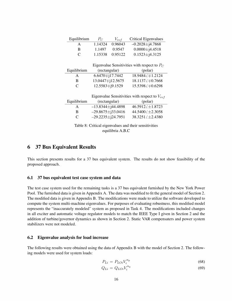
Equilibrium PC Vref Critical EigenvaluesA 1.14324 0.96043 �0.2028±j4.7868B 1.1497 0.9547 0.0000±j4.4518C 1.15338 0.95122 0.1523±j4.3125

Eigenvalue Sensitivities with respect to PCEquilibrium (rectangular) (polar)

A 6.6470∓j17.7442 18.94846 ∓1.2124B 13.0447∓j12.5675 18.1137 6 ∓0.7668C 12.5583∓j9.1529 15.5398 6 ∓0.6298

Eigenvalue Sensitivities with respect to VrefEquilibrium (rectangular) (polar)

A �13.8344±j44.4898 46.59126 ±1.8723B �29.8675±j33.0416 44.5400 6 ±2.3058C �29.2235±j24.7951 38.3251 6 ±2.4380

Table 8: Critical eigenvalues and their sensitivitiesequilibria A,B,C

6 37 Bus Equivalent Results

This section presents results for a 37 bus equivalent system. The results do not show feasibility of theproposed approach.

6.1 37 bus equivalent test case system and data

The test case system used for the remaining tasks is a 37 bus equivalent furnished by the New York PowerPool. The furnished data is given in Appendix A. The data was modi"ed to "t the general model of Section 2.The modi"ed data is given in Appendix B. The modi"cations were made to utilize the software developed tocompute the system multi-machine eigenvalues. For purposes of evaluating robustness, this modi"ed modelrepresents the �inaccurately modeled� system as proposed in Task 4. The modi"cations included changesin all exciter and automatic voltage regulator models to match the IEEE Type I given in Section 2 and theaddition of turbine/governor dynamics as shown in Section 2. Static VAR compensaters and power systemstabilizers were not modeled.

6.2 Eigenvalue analysis for load increase

The following results were obtained using the data of Appendix B with the model of Section 2. The follow-ing models were used for system loads:

PLi = PLOiVnpi (68)

QLi = QLOiVnqi (69)

16

For constant power loads (np = 0, nq = 0), the system was unstable with the following modes in theright-half plane:

+1.92± j3.01+0.13± j3.69

For constant current loads (np = 1, nq = 1), the system was stable (all eigenvalues in the left-half plane).The two modes of interest from above were,

−.0029± j5.03−.0009± j2.531

To examine the impact of increasing load, the load data of Appendix B was considered 100%. The realpower output of each generator and the real and reactive powers of each load were increased by a factor toindicate load growth with corresponding generation increase. At a percent loading of 101% (with np = nq =1), the system became unstable with the following eigenvalues in the right-half plane:

+.0248± j4.99+.0010± j2.52

Attempts to stabilize the system using operator controls were only partially successful. The software forcomputing the eigenvalue sensitivities did not produce reliable results. Participation factors were used toguide the choice of possible effective controls. Increasing the output of generator 2 by 1% gave the followingeigenvalues:

+.0101± j5.008+.0088± j2.52

This indicates that raising the output of generator 2 might stabilize one mode. Using this predicted sensitiv-ity, a 3% increase in generator 2 output gave the following eigenvalues:

−.022± j5.04+.024± j2.51

The eigenvalues moved as predicted, stabilizing the "rst mode, but destabilizing the second. Lowering theoutput to 98% of its initial value gave the following eigenvalues:

+.050± j4.94−.015± j2.52

Again, the eigenvalues moved as predicted, stabilizing the second mode, but destabilizing the "rst.

6.3 Eigenvalue analysis - line outage

The following results were obtained using the data of Appendix B with the model of Section 2. Simulationof the system showed that load #ow convergence was lost for a large number of line outages. Outage of line15-19 did not cause load #ow divergence and resulted in the following unstable modes (100% load, np = nq= 1):

+.0707± j4.72+.0036± j2.53

17

Attempts to stabilize the system using operator controls were partially successful. Lowering the output ofgenerator 2 to 98% resulted in the following eigenvalues:

+.0656± j4.65−.0113± j2.54

The "rst eigenvalue moved slightly to the left and the second was stabilized as in the last section. Loweringgenerator 2 further to 96% gave the following eigenvalues:

+0.0545± j4.56−.0263± j2.54

Lowering generator 2 further to 92% gave the following eigenvalues:

+.0744± j4.3−.0534± j2.54

The linear prediction in the movement of the "rst eigenvalue has failed. This 8% reduction caused theeigenvalue to reverse direction and become more unstable.

7 Computational Issues

Based on our experience with the 37 bus equivalent system, the computational requirements for computingeigenvalue sensitivities to operator control parameters will be very intense. The reason for this is primarilyin the need to compute all of the Hessian matrices associated with the sensitivity of the operating point. Thisis equivalent to computing N load #ow Jacobians for an N -bus system. While numerical sensitivities maybe feasible using incremental parameter changes with corresponding incremental eigenvalue changes, thisalso has computational issues. Each incremental change would require the computation of the equilibriumpoint for "xed operator controls. This is not a standard load #ow, and such software is not commerciallyavailable.

Timing runs on a Sun workstation indicate that it takes about 6 minutes to compute a subset of eigen-values on a 4000 bus system. A numerical sensitivity would require at least two such solutions for eachoperator control. Assuming an operator has over 100 possible controls, this means the computation time ona Sun workstation would take 2 × 6 × 100 = 1,200 minutes (20 hours). Even with advances in computingsoftware and hardware, this does not appear feasible for the near future.

8 Conclusions

The concept of using eigenvalue sensitivities to predict proper operator controls was shown to be viable ona single machine/in"nite bus test case. Every aspect of the analysis from analytical sensitivities throughnonlinear simulation indicated that the basic approach to avoidance and elimination of sustained oscillationsis feasible. In the 37 bus equivalent test case the results showed that there can be situations where theeigenvalue sensitivity information is unreliable. It is unreliable because the necessary controls predictedmay be too large to be in the region where linear prediction is accurate. Furthermore, instabilities can occur

18

with multiple modes in the right-half plane and operator controls which stabilize one mode can destablizeanother. This means that any ranking of controls must consider the impact of the control on all eigenvalues,not just the one or two that show an instability. Computational issues indicate that the time needed tocompute all operator-control options will be very large. After this phase of the investigation, we cannotclaim that the approach is feasible. We will continue our investigation into these issues without furtherfunding requests. Should any reliable solutions to these problems emerge, we will provide the results to allinterested persons in ESEERCO and NYSEG.

References

[1] E.H. Abed, P.P. Varaiya, �Nonlinear oscillations in power systems,� International Journal of ElectricEnergy and Power Systems, vol. 6, no. 1, Jan. 1984, pp. 37-43.

[2] R. T. Byerly, R. J. Bennon and D. E. Sherman, �Eigenvalue analysis of synchronizing power #owoscillations in large electric power systems,� IEEE Transactions on Power Apparatus and Systems,vol. PAS-101, January 1982, pp. 235-243.

[3] R. C. Burchett and G. T. Heydt, �Probabilistic methods for power system dynamic stability studies,�IEEE Transactions on Power Apparatus and Systems, vol. PAS-97, no. 3, May/June 1978, pp. 695-702.

[4] J.H. Chow, A. Gebreselassie, Dynamic voltage stability of a single machine constant power load sys-tem, 29th IEEE CDC conference, Honolulu HI, Dec. 1990, pp. 3057-3062.

[5] I. Dobson, L. Lu, Computing an optimum direction in control space to avoid saddle node bifurcationand voltage collapse in electric power systems, IEEE Transactions on Automatic Control, vol 37, no.10, October 1992, pp. 1616-1620.

[6] I. Dobson, Fernando Alvarado and C. L. DeMarco, �Sensitivity of Hopf bifurcations to power systemparameters,� Proceedings of the 31st Conference on Decision and Control, Tucson, Arizona, December1992.

[7] I. Dobson, Computing a closest bifurcation instability in multidimensional parameter space, Journal ofNonlinear Science, vol. 3, no. 3, 1993, pp. 307-327.

[8] G. Golub, C. VanLoan, Matrix Computations, Johns Hopkins Universtiy Press, Baltimore, 1983.

[9] G. Gross, C. F. Imparato and P. M. Look, �A tool for the comprehensive analysis of power systemdynamic stability,� IEEE Transactions on Power Apparatus and Systems, vol. PAS-101, no. 1, January1982.

[10] P. Kundur, G. J. Rogers, D. Y. Wong, L. Wang and M. G. Lauby, �A comprehensive computer programpackage for small signal stability analysis of power systems,� IEEE Transactions on Power Systems,vol. PWRS-5, no. 4, November 1990, pp. 1076-1083.

[11] D. M. Lam, H. Yee and B. Campbell, �An ef"cient improvement of the AESOPS algorithm for powersystem eigenvalue calculation,� IEEE Transactions on Power Systems, vol. 9, no. 4, November 1994,pp. 1880-1885.

19

[12] N. Martins, �Ef"cient eigenvalue and frequency response methods applied to power system small-signal stability studies,� IEEE Transactions on Power Systems, vol. PWRS-1, no. 1, 1986, pp. 217-226.

[13] J. E. Van Ness, J. M. Boyle and F. P. Imad, �Sensitivities of large multi-loop control systems,� IEEETransactions on Automatic Control, vol. AC-10, 1965, pp. 308-318.

[14] P. Nolan, N. Sinha and R. Alden, �Eigenvalue sensitivities of power systems including network andshaft dynamics,� IEEE Transactions on Power Apparatus and Systems, PAS-95, pp. 1318-1324, 1976.

[15] F. L. Pagola, I. J. Perez-Arriaga and G. C. Verghese, �On sensitivities, residues and participants: Ap-plications to oscillatory stability analysis and control,� IEEE Transactions on Power Systems, vol.PWRS-4, no. 1, 1989, pp. 278-285.

[16] M. A. Pai, K. R. Padiyar and P. S. Shetty, �Sensitivity based selection of control parameters for multi-machine power systems,� Abstract in IEEE Transactions on Power Apparatus and Systems, PAS-99,1980, p. 1320.

[17] P. W. Sauer, C. Rajagopalan and M. A. Pai, �An explanation and generalization of the AESOPS andPEALS algorithms,� IEEE Transactions on Power Systems, vol. 6, no. 1, February 1991, pp. 293-299.

[18] R. Seydel, From equilibrium to chaos: practical bifurcation and stability analysis, Elsevier, New YorkOR the second edition Springer-Verlag, New York, 1994.

[19] Thomas Smed, �Feasible eigenvalue sensitivity for large power systems,� IEEE Transactions on PowerSystems, vol. 8, no. 2, May 1993, pp. 555-563.

[20] N. Uchida and T. Nagao, �A new eigen-analysis method of steady-state stability studies for large powersystems: S matrix method,� IEEE Transactions on Power Systems, PWRS-3, no. 2, May 1988, pp.706-714.

[21] L. Wang and A. Semlyen, �Application of sparse eigenvalue techniques to the small signal stabilityanalysis of large power systems,� IEEE Transactions on Power Systems, vol. PWRS-5, pp. 635-642,May 1990.

[22] D. Y. Wong, G. J. Rogers, B. Poretta and P. Kundur, �Eigenvalue analysis of very large power systems,�IEEE Transactions on Power Systems, PWRS-3, no. 2, pp. 472-480, May 1988.

[23] L. Xu and S. Ahmed-Zaid, �Tuning of power system controllers using symbolic eigensensitivity anal-ysis and linear programming,� IEEE Transactions on Power Systems, vol. 10, no. 1, Feb. 1995, pp.314-321.

[24] EPRI Final Report, �Application of taxonomy theory,� Part I: Research Project 3573-10, April 1995,prepared byWashington University in St. Louis, System Science andMathematics, St. Louis, Missouri.

[25] E. Zhou, S. Chen, Y. Ni and B. Zhang, �Modi"ed selective analysis method and its application in theanalysis of power system dynamics,� IEEE Transactions on Power Systems, vol. 6, no. 3, August 1991,pp. 1189-1195.

20

A Appendix A

The attached pages list the 37 bus equivalent data in PTI raw format.

THE FOLLOWING PAGES MAY BE OBTAINED FROM THE AUTHORS

21

B Appendix B

The attached pages list the modi"ed 37 bus equivalent data in format for the University of Illinois simulation.

In order to run this model with the software being used at the University of Illinois it was necessary torenumber the system buses as shown below:

UI# NYPP#

1 43052 13 514 1365 14596 24587 28128 28339 283410 285511 286412 351713 352014 352315 364516 381417 461118 465619 489520 552521 589022 590223 590324 632125 659726 663227 665928 666029 948430 137731 386432 438333 438734 550635 568536 568637 6188

THE FOLLOWING PAGES MAY BE OBTAINED FROM THE AUTHORS

22