Electronic copy available at: http://ssrn.com/abstract=1411367 Rational Attention Allocation Over the Business Cycle Marcin Kacperczyk ∗ Stijn Van Nieuwerburgh † Laura Veldkamp ‡ November 15, 2011 § ∗ Department of Finance Stern School of Business and NBER, New York University, 44 W. 4th Street, New York, NY 10012; [email protected]; http://www.stern.nyu.edu/∼mkacperc. † Department of Finance Stern School of Business, NBER, and CEPR, New York University, 44 W. 4th Street, New York, NY 10012; [email protected]; http://www.stern.nyu.edu/∼svnieuwe. ‡ Department of Economics Stern School of Business, NBER, and CEPR, New York University, 44 W. 4th Street, New York, NY 10012; [email protected]; http://www.stern.nyu.edu/∼lveldkam. § We thank John Campbell, Joseph Chen, Xavier Gabaix, Vincent Glode, Ralph Koijen, Jeremy Stein, Matthijs van Dijk, and seminar participants at NYU Stern (economics and finance), Harvard Business School, Chicago Booth, MIT Sloan, Yale SOM, Stanford University (economics and finance), University of California at Berkeley (economics and finance), UCLA economics, Duke economics, University of Toulouse, University of Vienna, Australian National University, University of Melbourne, University of New South Wales, University of Sydney, University of Technology Sydney, Erasmus University, University of Mannheim, University of Alberta, Concordia, Lugano, the Amsterdam Asset Pricing Retreat, the Society for Economic Dynamics meetings in Istanbul, CEPR Financial Markets conference in Gerzensee, UBC Summer Finance conference, and Econometric Society meetings in Atlanta for useful comments and suggestions. Thank you to Isaac Baley for outstanding research assistance. Finally, we thank the Q-group for their generous financial support.

Welcome message from author
This document is posted to help you gain knowledge. Please leave a comment to let me know what you think about it! Share it to your friends and learn new things together.
Transcript
Electronic copy available at: http://ssrn.com/abstract=1411367
Rational Attention Allocation Over the
Business Cycle
Marcin Kacperczyk∗ Stijn Van Nieuwerburgh† Laura Veldkamp‡
November 15, 2011§
∗Department of Finance Stern School of Business and NBER, New York University, 44 W. 4th Street,
New York, NY 10012; [email protected]; http://www.stern.nyu.edu/∼mkacperc.†Department of Finance Stern School of Business, NBER, and CEPR, New York University, 44 W. 4th
Street, New York, NY 10012; [email protected]; http://www.stern.nyu.edu/∼svnieuwe.‡Department of Economics Stern School of Business, NBER, and CEPR, New York University, 44 W.
4th Street, New York, NY 10012; [email protected]; http://www.stern.nyu.edu/∼lveldkam.§We thank John Campbell, Joseph Chen, Xavier Gabaix, Vincent Glode, Ralph Koijen, Jeremy Stein,
Matthijs van Dijk, and seminar participants at NYU Stern (economics and finance), Harvard Business
School, Chicago Booth, MIT Sloan, Yale SOM, Stanford University (economics and finance), University of
California at Berkeley (economics and finance), UCLA economics, Duke economics, University of Toulouse,
University of Vienna, Australian National University, University of Melbourne, University of New South
Wales, University of Sydney, University of Technology Sydney, Erasmus University, University of Mannheim,
University of Alberta, Concordia, Lugano, the Amsterdam Asset Pricing Retreat, the Society for Economic
Dynamics meetings in Istanbul, CEPR Financial Markets conference in Gerzensee, UBC Summer Finance
conference, and Econometric Society meetings in Atlanta for useful comments and suggestions. Thank you
to Isaac Baley for outstanding research assistance. Finally, we thank the Q-group for their generous financial
support.

Electronic copy available at: http://ssrn.com/abstract=1411367
Abstract
The literature assessing whether mutual fund managers have skill typically regards skill
as an immutable attribute of the manager or the fund. Yet, many measures of skill, such
as returns, alphas, and measures of stock-picking and market-timing, appear to vary
over the business cycle. Because time-varying ability seems far-fetched, these results
call into question the existence of skill itself. This paper offers a rational explanation,
arguing that skill is a general cognitive ability that can be applied to different tasks,
such as picking stocks or market timing. Using tools from the rational inattention
literature, we show that the relative value of these tasks varies cyclically. The model
generates indirect predictions for the dispersion and returns of fund portfolios that
distinguish this explanation from others and which are supported by the data. In
turn, these findings offer useful evidence to support the notion of rational attention
allocation.

“What information consumes is rather obvious: It consumes the attention of its re-
cipients. Hence a wealth of information creates a poverty of attention, and a need
to allocate that attention efficiently among the overabundance of information sources
that might consume it.” Simon (1971)
The literature that evaluates skills of mutual fund managers typically regards skill as an
immutable attribute of the manager or the fund.1 Yet, many skill measures vary over the
business cycle, such as returns, alphas (Glode 2011), and measures of stock-picking and
market-timing (Kacperczyk, Van Nieuwerburgh, and Veldkamp 2011) (hereafter “KVV”).
Because time-varying ability seems far-fetched, these results call into question the existence
of skill itself. This paper examines a rational explanation for time-varying skill, where skill
is a general cognitive ability that can be applied to different tasks, such as picking stocks or
market timing, at different points in time. Each period, skilled managers choose how much
of their time or cognitive ability (call that “attention”) to allocate to each task. When the
economic environment changes, the relative payoffs of paying attention to market timing and
stock selection shift. The resulting fluctuations in attention allocation look like time-varying
skill. While this story might sound plausible, it leaves open three questions. First, why
would a manager want his attention allocation to depend on the state of the business cycle?
Second, do the manager’s attention choices exhibit the same pattern as the time-varying
skill observed in the data? If managers want to allocate more attention to stock-picking
in booms, do we see better stock picking in booms? Third, if there are many skilled and
unskilled managers in an asset market, would the time-series and cross-sectional portfolio and
return patterns resemble those in the data? This paper builds a simple theory of attention
allocation and portfolio choice and subjects it to these three tests.
The model uses tools from the rational inattention literature (Sims 2003) to analyze
the trade-off between allocating attention to each task. In recessions, the abundance of
aggregate risk and its high price both work in the same direction to make market timing
more valuable. The model generates indirect predictions for the dispersion and returns
of fund portfolios that distinguish this explanation from other potential explanations for
time-varying skill. It reveals that when skilled managers devote more time to market timing,
portfolio dispersion is higher, both among skilled managers and between skilled and unskilled
1For theoretical models, see e.g., Mamaysky and Spiegel (2002), Berk and Green (2004), Kaniel andKondor (2010), Cuoco and Kaniel (2010), Vayanos and Woolley (2010), Chien, Cole, and Lustig (2010),Chapman, Evans, and Xu (2010), and Pastor and Stambaugh (2010). A number of recent papers in theempirical mutual fund literature also find that some managers have skill, e.g., Kacperczyk, Sialm, and Zheng(2005, 2008), Kacperczyk and Seru (2007), Cremers and Petajisto (2009), Huang, Sialm, and Zhang (2011),Koijen (2010), and Baker, Litov, Wachter, and Wurgler (2010).
1

managers. It predicts that recessions are times when skilled managers outperform others by
a larger margin. Finally, it predicts that volatility and recessions should each have an
independent effect on attention, dispersion, and performance. All of these predictions are
borne out in the mutual fund data.
These findings offer useful evidence to support a variety of theories that use rational
attention allocation to explain phenomena in many economic environments. Recent work
has shown that introducing attention constraints into decision problems can help explain ob-
served consumption, price-setting, and investment patterns as well as the timing of govern-
ment announcements and the propensity for governments to be unprepared for rare events.2
An obstacle to the progress of this line of work is that information is not directly observable,
precluding a direct test of whether decision makers actually allocate their attention in a
value-maximizing way. While papers such as Klenow and Willis (2007), Mondria, Wu, and
Zhang (2010) and Mackowiak, Moench, and Wiederholt (2009) have also tested predictions
of rational inattention models, none has looked for evidence that attention is reallocated,
arguably a more stringent test of the theory.
To surmount the problem that attention is unobservable, our model uses an observable
variable – the state of the business cycle – to predict attention allocation. Attention, in turn,
predicts aggregate investment patterns. Because the theory begins and ends with observable
variables, it becomes testable. To carry out these tests, we use data on actively managed
equity mutual funds. A wealth of detailed data on portfolio holdings and returns makes
this industry an ideal setting in which to test whether decision makers allocate attention
optimally.
To explore whether a rational attention allocation can explain the behavior of mutual
fund managers, we build a general equilibrium model in which a fraction of investment
managers have skill. These skilled managers can observe a fixed number of signals about
asset payoffs and choose what fraction of those signals will contain aggregate versus stock-
specific information. We think of aggregate signals as macroeconomic data that affect future
cash flows of all firms, and of stock-specific signals as firm-level data that forecast the part of
firms’ future cash flows that is independent of the aggregate shocks. Based on their signals,
skilled managers form portfolios, choosing larger portfolio weights for assets that are more
2See, for example, Sims (2003) on consumption, Mackowiak and Wiederholt (2009a, 2009b), and Matejka(2011) on price setting, and Van Nieuwerburgh and Veldkamp (2009, 2010) and Kondor (2009) on financialinvestment. Reis (2011) considers the optimal timing of government announcements and Mackowiak andWiederholt (2011) use rational inattention constraint to model the allocation of cognitive energy to planningfor rare events. A related attention constraint called inattentiveness is explored in Reis (2006). Veldkamp(2011) provides a survey of this literature.
2

likely to have high returns.
The model produces four main predictions. The first prediction is that attention should
be reallocated over the business cycle. In the data, recessions are times when unexpected
returns are low, aggregate volatility rises, and the price of risk surges. When we embed
these three forces in our model, the first has little effect on attention allocation, but the
second and third forces both draw attention to aggregate shocks in recessions. The increased
volatility of aggregate shocks makes it optimal to allocate more attention to them, because
it is more valuable to pay attention to more uncertain outcomes. The elevated price of risk
amplifies this reallocation: Since aggregate shocks affect a large fraction of the portfolio’s
value, paying attention to aggregate shocks resolves more portfolio risk than learning about
stock-specific risks. When the price of risk is high, such risk-minimizing attention choices
become more valuable. While the idea that it is more valuable to shift attention to more
volatile shocks may not be all that surprising, whether changes in the price of risk would
amplify or counteract this effect is not obvious.
The second and third predictions do not come from the reallocation of attention. Rather,
they help to distinguish this theory from non-informational alternatives and support the idea
that at least some portfolio managers are engaging in value-maximizing behavior. The sec-
ond prediction is counter-cyclical dispersion in portfolio holdings and profits. In recessions,
when aggregate shocks to asset payoffs are larger in magnitude, asset payoffs exhibit more co-
movement. Thus, any portfolio strategies that put exogenously fixed weights on assets would
have returns that also comove more in recessions. In contrast, when investment managers
learn about asset payoffs and manage their portfolios according to what they learn, fund
returns comove less in recessions. The reason is that when aggregate shocks become more
volatile, managers who learn about aggregate shocks put less weight on their common prior
beliefs, which have less predictive power, and more weight on their heterogeneous signals.
This generates more heterogeneous beliefs in recessions and therefore more heterogeneous
investment strategies and fund returns.
Third, the model predicts time variation in fund performance. Since the average fund
can only outperform the market if there are other, non-fund investors who underperform, the
model also includes unskilled non-fund investors. Because asset payoffs are more uncertain,
recessions are times when information is more valuable. Therefore, the informational ad-
vantage of the skilled over the unskilled increases and generates higher returns for informed
managers. The average fund’s outperformance rises.
The fourth prediction is perhaps the most specific to our theory. It argues that all three
3

of the above effects of recessions come in part from high aggregate volatility, and in part
from the high price of risk. Therefore, periods of high aggregate volatility should be periods
in which attention is allocated to aggregate shocks, portfolio dispersion is high, and skilled
funds outperform. Then, after controlling for volatility, there should also be an additional
positive effect of recessions on all three measures. This additional effect comes from the fact
that recessions are also times when the price of risk is high. In other words, both volatility
and the price of risk have separate effects on skill, dispersion, and performance.
We test the model’s four main predictions on the universe of actively managed U.S.
mutual funds. To test the first prediction, a key insight is that managers can only choose
portfolios that covary with shocks they pay attention to. Thus, to detect cyclical changes
in attention, we should look for changes in covariances. KVV does precisely this. They
estimate the covariance of each fund’s portfolio holdings with the aggregate payoff shock,
proxied by innovations in industrial production growth. This covariance measures a man-
ager’s ability to time the market by increasing (decreasing) her portfolio positions in antici-
pation of good (bad) macroeconomic news. This timing covariance rises in recessions. KVV
also calculate the covariance of a fund’s portfolio holdings with asset-specific shocks, prox-
ied by innovations in earnings. This covariance measures managers’ ability to pick stocks
that subsequently experience unexpectedly high earnings. Consistent with the theory, this
stock-picking covariance increases in expansions.
Second, we test for cyclical changes in portfolio dispersion. We find that, in recessions,
funds hold portfolios that differ more from one another. As a result, their cross-sectional
return dispersion increases, consistent with the theory. In the model, much of this dispersion
comes from taking different bets on market outcomes, which should show up as dispersion
in CAPM betas. We indeed find evidence in the data for higher beta dispersion in recessions
as well.
Third, we document fund outperformance in recessions.3 Risk-adjusted excess fund re-
turns (alphas) are around 1.8 to 2.4% per year higher in recessions, depending on the spec-
ification. Gross alphas (before fees) are not statistically different from zero in expansions,
but they are positive (2.1%) in recessions.4 These cyclical differences are statistically and
3Empirical work by Moskowitz (2000), Kosowski (2006), Lynch and Wachter (2007), and Glode (2011)also documents such evidence, but their focus is solely on performance, not on managers’ attention allocationnor their investment strategies. Furthermore, these studies are silent on the specific mechanism that drivesthe outperformance result, which is one of the main contributions of our paper.
4Net alphas (after fees) are negative in expansions (-0.9%) and positive (1.0%) in recessions. Since fundsdo not set fees in our model, we have no predictions about after-fee alphas. For a theory about why weshould expect net alphas to be zero, see Berk and Green (2004).
4

economically significant.
Fourth, we document an effect of recessions on covariance, dispersion, and performance,
above and beyond that which comes from volatility alone. When we use both a recession
indicator and aggregate volatility as explanatory variables, we find that both contribute
about equally to our three main results. Showing that these results are truly business-cycle
phenomena – as opposed to merely high volatility phenomena – is interesting because it
connects these results with the existing macroeconomics literature on rational inattention,
e.g., Mackowiak and Wiederholt (2009a, 2009b).
The rest of the paper is organized as follows. Section 1 lays out our model. After
describing the setup, we characterize the optimal information and investment choices of
skilled and unskilled investors. We show how equilibrium asset prices are formed. We derive
theoretical predictions for funds’ attention allocation, portfolio dispersion, and performance.
Section 2 tests the model’s predictions using the context of actively managed mutual funds.
Section 3 discusses alternative explanations. We conclude that while a handful of theories
could explain one or two of the facts we document, few, if any, alternatives would explain
why covariance, dispersion, and performance all vary both with macroeconomic volatility
and with recessions.
1 Model
We develop a stylized model whose purpose is to understand how the optimal attention
allocation of investment managers depends on the business cycle and how attention affects
asset holdings and asset prices. Most of the complexity of the model comes from the fact
that it is an equilibrium model. But in order to study the effects of attention on asset
holdings, asset prices and fund performance, having an equilibrium model is a necessity.
The equilibrium model makes it clear that, while investors might all pay more attention to
a particular asset, they cannot all hold more of that asset, because the market must clear.
Similarly, an equilibrium model ensures that for every investor that outperforms, there is
someone who underperforms as well.
1.1 Setup
We consider a three-period model. At time 1, skilled investment managers choose how to
allocate their attention across aggregate and asset-specific shocks. At time 2, all investors
choose their portfolios of risky and riskless assets. At time 3, asset payoffs and utility are
5

realized. Since this is a static model, the investment world is either in the recession (R) or
in the expansion state (E).5
Assets The model features three assets. Assets 1 and 2 have random payoffs f with
respective loadings b1, b2 on an aggregate shock a, and face stock-specific shocks s1, s2. The
third asset, c, is a composite asset. Its payoff has no stock-specific shock and a loading of
one on the aggregate shock. We use this composite asset as a stand-in for all other assets to
avoid the curse of dimensionality in the optimal attention allocation problem. Formally,
fi = µi + bia+ si, i ∈ {1, 2}
fc = µc + a
where the shocks a ∼ N(0, σa) and si ∼ N(0, σi), for i ∈ {1, 2}. At time 1, the distribution of
payoffs is common knowledge; all investors have common priors about payoffs f ∼ N(µ,Σ).
Let E1, V1 denote expectations and variances conditioned on this information. Specifically,
E1[fi] = µi. The prior covariance matrix of the payoffs, Σ, has the following entries: Σii =
b2iσa + σi and Σij = bibjσa. In matrix notation:
Σ = bb′σa +
σ1 0 0
0 σ2 0
0 0 0
where the vector b is defined as b = [b1 b2 1]
′. In addition to the three risky assets, there
exists a risk-free asset that pays a net return, r.
Investors We consider a continuum of atomless investors. In the model, the only ex-ante
difference between investors is that a fraction χ of them have skill, meaning that they can
choose to observe a set of informative signals about the payoff shocks a or si. We call these
investors skilled mutual funds and describe their signal choice problem below. The remaining
unskilled investors observe no information other than their prior beliefs.
Some of the unskilled investors are mutual fund managers. As in reality, there are also
5We do not consider transitions between recessions and expansions, although such an extension would beeasy in our setting because assets are short lived and their payoffs are realized and known to all investorsat the end of each period. Thus, a dynamic model would amount to a succession of static models that areeither in the expansion or in the recession state.
6

non-fund investors. We assume that they are unskilled.6 The reason for modeling non-
fund investors is that without them, the sum of all funds’ holdings would have to equal the
market (market clearing) and therefore, the average fund return would have to equal the
market return. There could be no excess return in expansions or recessions.
Bayesian Updating At time 2, each skilled investment manager observes signal realiza-
tions. Signals are random draws from a distribution that is centered around the true payoff
shock, with a variance equal to the inverse of the signal precision that was chosen at time
1. Thus, skilled manager j’s signals are ηaj = a + eaj, η1j = s1 + e1j, and η2j = s2 + e2j,
where eaj ∼ N(0, K−1aj ), e1j ∼ N(0, K−1
1j ), and e2j ∼ N(0, K−12j ) are independent of each
other and across fund managers. Managers combine signal realizations with priors to update
their beliefs, using Bayes’ law.
Of course, asset prices contain payoff-relevant information as well. Lemma 2 in Appendix
A establishes that managers always prefer to process additional private signals, rather than
to use the same amount of capacity to process the information in prices. Therefore, we model
managers as if they observed prices, but did not exert the mental effort required to infer the
payoff-relevant signals.7
Since the resulting posterior beliefs (conditional on time-2 information) are such that
payoffs are normally distributed, they can be fully described by posterior means, (aj, sij),
and variances, (σaj, σij). More precisely, posterior precisions are the sum of prior and signal
precisions: σ−1aj = σ−1
a + Kaj and σ−1ij = σ−1
i + Kij. The posterior means of the stock-
specific shocks, sij, are a precision-weighted linear combination of the prior belief that si = 0
and the signal ηi: sij = Kijηij/(Kij + σ−1i ). Simplifying yields sij = (1 − σijσ
−1i )ηij and
aj = (1 − σajσ−1a )ηaj. Next, we convert posterior beliefs about the underlying shocks into
posterior beliefs about the asset payoffs. Let Σj be the posterior variance-covariance matrix
of payoffs f :
Σj = bb′σaj +
σ1j 0 0
0 σ2j 0
0 0 0
6For our results, it is sufficient to assume that the fraction of non-fund investors that are unskilled is
higher than that for the investment managers (funds).7We could allow managers to infer this information and subtract the amount of attention required to
infer this information from their total attention endowment. That would not change the basic result thatinvestors prefer to learn more about more volatile risks (see Van Nieuwerburgh and Veldkamp (2009)).
7

Likewise, let µj be the 3× 1 vector of posterior expected payoffs:
µj = [µ1 + b1aj + s1j, µ2 + b2aj + s2j, µc + aj]′ (1)
For any unskilled manager or investor: µj = µ and Σj = Σ.
Modeling recessions The asset pricing literature identifies three principal effects of re-
cessions: (1) returns are unexpectedly low, (2) returns are more volatile, and (3) the price of
risk is high. Section 2.2 discusses the empirical evidence supporting the latter two effects. To
capture the return volatility effect (2) in the model, we assume that the prior variance of the
aggregate shock in recessions (R) is higher than the one in expansions (E): σa(R) > σa(E).
To capture the varying price of risk (3), we vary the parameter that governs the price of
risk, which is risk aversion. We assume ρ(R) > ρ(E). We continue to use σa and ρ to denote
aggregate shock variance and risk aversion in the current business cycle state.
The first effect of recessions, unexpectedly low returns, cannot affect attention allocation
because attention must be allocated before returns are observed. Yet, unexpected returns
could affect managers’ return covariances. The difficulty in analyzing this effect is that since
agents in our model always know the current state of the business cycle, they cannot be
systematically surprised by low asset payoffs in recessions. When low payoffs are expected,
asset prices fall, leaving returns unaffected. Therefore, exploring (1) requires a slightly
modified model that relaxes rational expectations. The Supplementary Appendix explores
this model numerically and shows that the unexpectedly low returns have little effect on the
results.8 The main body of the paper explores the volatility and price of risk effects.
Portfolio Choice Problem We solve this model by backward induction. We first solve
for the optimal portfolio choice at time 2 and substitute in that solution into the time-1
optimal attention allocation problem.
Investors are each endowed with initial wealth, W0. They have mean-variance preferences
over time-3 wealth, with a risk-aversion coefficient, ρ. Let E2 and V2 denote expectations
and variances conditioned on all information known at time 2. Thus, investor j chooses qj
to maximize time-2 expected utility, U2j:
U2j = ρE2[Wj]−ρ2
2V2[Wj] (2)
8The supplementary appendix is a separate document, not intended for publication.
8

subject to the budget constraint:
Wj = rW0 + q′j(f − pr.) (3)
Since there are no wealth effects with exponential utility, we normalize W0 to zero for the
theoretical results. After having received the signals and having observed the prices of the
risky assets, p, the investment manager chooses risky asset holdings, qj, where p and qj are
3-by-1 vectors.
Asset Prices Equilibrium asset prices are determined by market clearing:∫qjdj = x+ x, (4)
where the left-hand side of the equation is the vector of aggregate demand and the right-
hand side is the vector of aggregate supply. As in the standard noisy rational expectations
equilibrium model, the asset supply is random to prevent the price from fully revealing the
information of informed investors. We denote the 3× 1 noisy asset supply vector by x+ x,
with a random component x ∼ N(0, σxI).
Attention Allocation Problem At time 1, a skilled investment manager j chooses the
precisions of signals about the payoff-relevant shocks a, s1, or s2 that she will receive at
time 2. We denote these signal precisions by Kaj, K1j, and K2j, respectively. These choices
maximize time-1 expected utility, U1j, over the fund’s terminal wealth:
U1j = E1
[ρE2[Wj]−
ρ2
2V2[Wj]
], (5)
subject to two constraints.
The first constraint is the information capacity constraint. It states that the sum of the
signal precisions must not exceed the information capacity:
K1j +K2j +Kaj ≤ K. (6)
Note that our model holds each manager’s total attention fixed and studies its allocation in
recessions and expansions. In Section 1.9, we allow a manager to choose how much capacity
for attention to acquire.
9

Unskilled investors have no information capacity, K = 0. In Bayesian updating with
normal variables, observing one signal with precision τ−1 or two signals, each with precision
τ−1/2, is equivalent. Therefore, one interpretation of the capacity constraint is that it
allows the manager to observe N signal draws, each with precision K/N , for large N . The
investment manager then chooses how many of those N signals will be about each shock.9
The second constraint is the no-forgetting constraint, which ensures that the chosen
precisions are non-negative:
K1j ≥ 0 K2j ≥ 0 Kaj ≥ 0. (7)
It prevents the manager from erasing any prior information, to make room to gather new
information about another shock.
1.2 Model Solution
Substituting the budget constraint (3) into the objective function (2) and taking the first-
order condition with respect to qj reveals that optimal holdings are increasing in the investor’s
risk tolerance, precision of beliefs, and expected return on the assets:
qj =1
ρΣ−1j (µj − pr). (8)
Since uninformed fund managers and non-fund investors have identical beliefs, µj = µ and
Σj = Σ, they hold identical portfolios ρ−1Σ−1(µ− pr).
Using the market-clearing condition (4), equilibrium asset prices are linear in payoffs and
supply shocks. We derive the linear coefficients A, B and C such that:
Lemma 1. p = 1r(A+Bf + Cx)
A detailed derivation of expected utility and the proofs of this and all further propositions
are in Appendix A.
Substituting optimal risky asset holdings from equation (8) into the first-period objective
function (5) yields: U1j = 12E1
[(µj − pr)Σ−1
j (µj − pr)]. Because asset prices are linear
functions of normally distributed payoffs and asset supplies, expected excess returns, µj−pr,
9The results are not sensitive to the additive nature of the information capacity constraint. They alsohold, for example, for a product constraint on precisions. The entropy constraints often used in informationtheory take this multiplicative form. Results available upon request.
10

are normally distributed as well. Therefore, (µj − pr)Σ−1j (µj − pr) is a non-central χ2-
distributed variable, with mean10
U1j =1
2trace(Σ−1
j V1[µj − pr]) +1
2E1[µj − pr]′Σ−1
j E1[µj − pr]. (9)
1.3 Bringing Model to Data
The following sections explain the model’s four key predictions: attention allocation, dis-
persion in investors’ portfolios, average performance, and the effect of recessions on these
objects beyond that of aggregate volatility. For each prediction, we state a hypothesis and
explain how we test it.
Our empirical measures use conventional definitions of asset returns, portfolio returns,
and portfolio weights. Risky asset returns are defined asRi ≡ fipi−1, for i ∈ {1, 2, c}, while the
risk-free asset return is R0 ≡ 1+r1
−1 = r. We define the market return as the value-weighted
average of the individual asset returns: Rm ≡∑
i∈{1,2,c}wmi R
i, where wmi ≡ piqi∑
k∈{1,2,c} pkqkand
qi ≡∫jqji is the total demand for asset j. Likewise, a fund j’s return is Rj ≡
∑i∈{0,1,2,c} w
jiR
i,
where wji ≡
piqji∑
k∈{0,1,2,c} pkqjk
. It follows that end-of-period wealth (assets under management)
equals beginning-of-period wealth times the fund return: W j = W j0 (1 +Rj).
1.4 Prediction 1: Cyclical Attention Re-allocation
First, we derive from the model the prediction that the optimal attention allocation in
expansions differs from that in recessions. Specifically, there should be more attention paid to
aggregate shocks in recessions and more attention paid to stock-specific shocks in expansions.
Recessions involve changes in the volatility of aggregate shocks and changes in the price of
risk. In order to see the effect of each aspect of a recession, we consider each separately,
beginning with the rise in volatility.
In the model, each skilled manager (K > 0) solves for the choice of signal precisions
Kaj ≥ 0 and K1j ≥ 0 that maximize her time-1 expected utility (9). The choice of signal
precision K2j ≥ 0 is implied by the capacity constraint (6). A first prediction of our model is
that it becomes relatively more valuable to learn about the aggregate shock, a, in recessions.
10If z ∼ N(E[z], V ar[z]), then E[z′z] = trace(V ar[z]) + E[z]′E[z], where trace is the matrix trace (the
sum of its diagonal elements). Setting z = Σ−1/2j (µj − pr) delivers the result.
11

Proposition 1. If price noise (σx) is sufficiently large (condition (42) holds), then the
marginal value of a given skilled investor j reallocating an increment of capacity from stock-
specific shock i ∈ {1, 2} to the aggregate shock is increasing in the aggregate shock variance:
If Kaj = K and Kij = K − K, then ∂2U/∂K∂σa > 0.
Intuitively, in most learning problems, investors prefer to learn about large shocks that are
an important component of the overall asset supply, and volatile shocks that have high prior
payoff variance. Aggregate shocks are larger in scale, but are less volatile than stock-specific
shocks. Recessions are times when aggregate volatility increases, which makes aggregate
shocks more valuable to learn about. The converse is true in expansions. Note that this is
a partial derivative result. It holds information choices fixed. In any interior equilibrium,
attention will be reallocated until the marginal utility of learning about aggregate and stock-
specific shocks is equalized. But it is the initial increase in marginal utility which drives this
re-allocation.
It would seem logical that learning about aggregate shocks should always be more valuable
in times when those shocks are more volatile. But working through the theory teaches us
that this is not true under all circumstances. When the parameter restriction (condition
(42)) is violated, more aggregate payoff risk (higher σa) creates less risk in expected returns
(lower V ar[f − pr]). This is possible when prices are very good at aggregating information
(low σx), when many agents acquire lots of information about the aggregate shock (high
Ka), and when risk aversion is low. This is a sufficient but not a necessary condition for
many of our results to hold. In our numerical work, when we choose parameter values that
replicate the observed volatility of aggregate stock market returns and simulate the model,
(42) is always easily satisfied.
Next, we consider the effect of an increase in the price of risk. The following result shows
that the increase in the price of risk induces managers to allocate even more attention to the
aggregate shock in recessions. The additional price of risk effect should show up as an effect
of recessions, above and beyond what aggregate volatility alone can explain. The parameter
that governs the price of risk in our model is risk aversion. The following result shows that
an increase in the price of risk (risk aversion) in recessions is an independent force driving
the reallocation of attention from stock-specific to aggregate shocks.
Proposition 2. If the size of the composite asset xc is sufficiently large, then an increase
in risk aversion increases the marginal utility of reallocating a unit of capacity from the
firm-specific shock to the aggregate shock: ∂2U/∂ρ∂(Kaj −K1j)) > 0.
12

The intuition for this result is that the aggregate shock affects a large fraction of the value
of one’s portfolio. Therefore, a marginal reduction in the uncertainty about an aggregate
shock reduces total portfolio risk by more than the same-sized reduction in the uncertainty
about a stock-specific shock. In other words, learning about the aggregate shock is the most
efficient way to reduce portfolio risk. The more risk averse an agent is, the more attractive
aggregate attention allocation becomes.
As long as the investor’s capacity allocation choice is not a corner solution (Kaj = 0
or Kaj = K), a rise in the marginal utility of aggregate shock information increases the
optimal Kaj. In these environments, skilled investment managers allocate a relatively larger
fraction of their attention to learning about the aggregate shock in recessions. But, that
effect can break down when assets become very asymmetric because corner solutions arise.
For example, if the average supply of the composite asset, xc, is too large relative to the
supply of the individual asset supplies, x1 and x2, the aggregate shock will be so valuable to
learn about that all skilled managers will want to learn about it exclusively (Kaj = K) in
expansions and recessions. Similarly, if the aggregate volatility, σa, is too low, then nobody
ever learns about the aggregate shock (Kaj = 0 always).
Investors’ optimal attention allocation decisions are reflected in their portfolio holdings.
In recessions, skilled investors predominantly allocate attention to the aggregate payoff shock,
a. They use the information they observe to form a portfolio that covaries with a. In times
when they learn that a will be high, they hold more risky assets whose returns are increasing
in a. This positive covariance can be seen from equation (8) in which q is increasing in µj
and from equation (1) in which µj is increasing in aj, which is further increasing in a. The
positive covariances between the aggregate shock and funds’ portfolio holdings in recessions,
on the one hand, and between stock-specific shocks and the portfolio holdings in expansions,
on the other hand, directly follow from optimal attention allocation decisions switching over
the business cycle. As such, these covariances are the key moments that enable us to test
the attention allocation predictions of the model.
Following KVV, we define a fund’s fundamentals-based timing ability, Ftiming, as the
covariance between its portfolio weights in deviation from the market portfolio weights,
wji −wm
i , and the aggregate payoff shock, a, over a T -period horizon, averaged across assets:
Ftimingjt =1
TN j
Nj∑i=1
T−1∑τ=0
(wjit+τ − wm
it+τ )(at+τ+1), (10)
where N j is the number of individual assets held by fund j. The subscript t on the portfolio
13

weights and the subscript t + 1 on the aggregate shock signify that the aggregate shock
is unknown at the time of portfolio formation. Relative to the market, a fund with a
high Ftiming overweights assets that have high (low) sensitivity to the aggregate shock
in anticipation of a positive (negative) aggregate shock realization and underweights assets
with a low (high) sensitivity.
When skilled investment managers allocate attention to stock-specific payoff shocks, si,
information about si allows them to choose portfolios that covary with si. Fundamentals-
based stock picking ability, Fpicking, hich measures the covariance of a fund’s portfolio
weights of each stock, relative to the market, with the stock-specific shock, si:
Fpickingjt =1
N j
Nj∑i=1
(wjit − wm
it )(sit+1). (11)
How well the manager can choose portfolio weights in anticipation of future asset-specific
payoff shocks is closely linked to her stock-picking ability.
Ftiming and Fpicking are closely related to commonly-used measures of market-timing
and stock-picking ability. Typical measures of market-timing ability estimate how a fund’s
holdings of each asset, relative to the market, covary with the systematic component of
the stock return, over the next T periods. Before the market return rises, market timers
overweight assets that have high betas. Likewise, they underweight assets with high betas
in anticipation of a market decline. Similarly, stock picking typically measures how a fund’s
holdings of each stock, relative to the market, covary with the idiosyncratic component of the
stock return. A fund that successfully picks stocks overweights assets that have subsequently
high idiosyncratic returns and underweights assets with low subsequent idiosyncratic returns.
The key difference between our measures and the conventional ones is that picking and
timing measure how a portfolio covaries with returns, while Fpicking and Ftiming mea-
sure how a portfolio covaries with aggregate and firm-specific fundamentals. KVV examine
the cyclical behavior of funds’ picking and timing ability, as measured in this more conven-
tional way and show that picking also rises in recessions and timing also rises in expansions,
just as Fpicking and Ftiming do. To test our theory as directly as possible, we use the
fundamentals-based measures because they correspond more closely to the idea in the model
that funds are learning about fundamentals and using signals about those fundamentals to
time the market and pick stocks.
14

1.5 Prediction 2: Dispersion
Since many studies detect no skill, perhaps the most controversial implication of the previous
finding is that investment managers are processing information at all. Our second and third
predictions speak directly to that implication.
In recessions, as aggregate shocks become more volatile, the firm-specific shocks to assets’
payoffs account for less of the variation, and the comovement in stock payoffs rises. Since
asset payoffs comove more, the payoffs to all investment strategies that put fixed weights on
assets should also comove more. But when investment managers are processing information,
this prediction is reversed. To see why, consider the Bayesian updating formula for the
posterior mean of asset payoffs. It is a weighted average of the prior mean µ and the fund
j’s signal ηj|f ∼ N(f,Ση), where each is weighted by their relative precision:
E[f |ηj] =(Σ−1 + Σ−1
η
)−1 (Σ−1µ+ Σ−1
η ηj)
(12)
In recessions, when the variance of the aggregate shock, σa, rises, the prior beliefs about asset
payoffs become more uncertain: Σ rises and Σ−1 falls. This makes the weight on prior beliefs
µ decrease and the weight on the signal ηj increase. The prior µ is common across agents,
while the signal ηj is heterogeneous. When informed managers weigh their heterogeneous
signals more, their resulting posterior beliefs become more different from each other and
more different from the beliefs of uninformed managers or investors. More disagreement
about asset payoffs results in more heterogeneous portfolios and portfolio returns.
Thus, the model’s second prediction is that in recessions, the cross-sectional dispersion in
funds’ investment strategies and returns should rise. The following Proposition shows that
funds’ portfolio holdings and returns, q′j(f − pr), display higher cross-sectional dispersion
when aggregate risk is higher, in recessions.
Proposition 3. If condition (42) holds, χK < σ−1a , then for given Kaj and Kij, an increase
in aggregate risk, σa, increases the dispersion of funds’ portfolios E[∑
iϵ{1,2,c}(qij − qi)2], and
their portfolio returns E[((qj − q)′(f − pr))2], where q ≡∫qjdj.
As before, the parameter restriction is sufficient, but not necessary, and is not very tight
when calibrated to the data.
Next, we consider the effect of an increase in the price of risk. The following result shows
that an increase in the price of risk increases the dispersion of portfolio returns.
15

Proposition 4. If the variance of asset supply shocks (σx) is sufficiently high (conditions
(56) and (57) hold), then for given Kaj, Kij ∀j , an increase in risk aversion ρ increases the
dispersion of funds’ portfolio returns E[((qj − q)′(f − pr))2].
The primary reason return dispersion increases is that a higher ρ increases the price of risk
and thus the average level of returns. Since the dispersion in returns is increasing in the level
of returns, return dispersion increases as well. But this effect has to offset a counter-acting
force. Recall that the optimal portfolio for investor j takes the form q = (1/ρσj)(µj−pr). If
ρ increases, the scale of q falls. The increase in returns needs to increase dispersion enough
to offset the decrease in dispersion coming from the effect of 1/ρ reducing q.
To connect this Proposition to the data, we measure portfolio dispersion as the sum of
squared deviations of fund j’s portfolio weight in asset i at time t, wjit, from the average
fund’s portfolio weight in asset i at time t, wmit , summed over all assets held by fund j, N j:
Portfolio Dispersionjt =Nj∑i=1
(wjit − wm
it
)2(13)
This measure is similar to the portfolio concentration measure in Kacperczyk, Sialm, and
Zheng (2005) and the active share measure in Cremers and Petajisto (2009). It is the same
quantity as in Proposition 3, except that the number of shares q is replaced with portfolio
weights w. Our numerical example shows that the model’s fund Portfolio Dispersion,
defined over portfolio weights w, is higher in recessions as well. In recessions, the portfolios
of the informed managers differ more from each other and more from those of the uninformed
investors. Part of this difference comes from a change in the composition of the risky asset
portfolio and part comes from differences in the fraction of assets held in riskless securities.
Fund j’s portfolio weight wjit is a fraction of the fund’s assets, including both risky and
riskless, held in asset i. Thus, when one informed fund gets a bearish signal about the market,
its wjit for all risky assets i falls. Dispersion can rise when funds take different positions in
the risk-free asset, even if the fractional allocation among the risky assets remains identical.
The higher dispersion across funds’ portfolio strategies translates into a higher cross-
sectional dispersion in fund abnormal returns (Rj − Rm). To facilitate comparison with
the data, we define the dispersion of variable X as |Xj − X|. The notation X denotes the
equally weighted cross-sectional average across all investment managers (excluding non-fund
investors).
When funds get signals about the aggregate state a that are heterogenous, they take
different directional bets on the market. Some funds tilt their portfolios to high-beta assets
16

and other funds to low-beta assets, thus creating dispersion in fund betas. To look for
evidence of this mechanism, we form a CAPM regression for fund j
Rjt = αj + βjRm
t + σjεεjt (14)
and test for an increase in the beta dispersion in recessions as well.
1.6 Prediction 3: Performance
The third prediction of the model is that the average performance of investment managers is
higher in recessions than it is in expansions. To measure performance, we want to measure
the portfolio return, adjusted for risk. One risk adjustment that is both analytically tractable
in our model and often used in empirical work is the certainty equivalent return, which is
also an investor’s objective (5). The following Proposition shows that the average certainty
equivalent of skilled funds’ returns exceeds that of unskilled funds or investors by more when
aggregate risk is higher, that is, in recessions.
Proposition 5. If (42) holds, then an increase in aggregate shock variance increases the
difference between an informed investor expected certainty equivalent return and the expected
certainty equivalent return of an uninformed investor: ∂(Uj − UU)/∂σa > 0.
Corollary 1 in Appendix A.9 shows that a similar result holds for (risk unadjusted)
abnormal portfolio returns, defined as the fund’s portfolio return, q′j(f − pr), minus the
market return, q′(f − pr).
Because asset payoffs are more uncertain, recessions are times when information is more
valuable. Therefore, the advantage of the skilled over the unskilled increases in recessions.
This informational advantage generates higher returns for informed managers. In equilib-
rium, market clearing dictates that alphas average to zero across all investors. However,
because the data only include mutual funds, our model calculations must similarly exclude
non-fund investors. Since investment managers are skilled or unskilled, while other investors
are only unskilled, an increase in the skill premium implies that an average manager’s risk-
adjusted return rises in recessions.
Next, we consider the effect of an increase in the price of risk on performance. The
following result shows that the average certainty equivalent of skilled funds’ returns exceeds
that of unskilled funds by more when the price of risk is higher, that is, in recessions.
17

Proposition 6. For given Kaj, K1j, K2j strictly positive, an increase in risk aversion ρ
for all investors increases the difference in expected certainty equivalent returns between an
informed and an uninformed investor: ∂(Uj − UU)/∂ρ > 0.
The reason that a higher price of risk leads to higher performance is that information can
resolve risk. Therefore, informed managers are compensated for risk that they do not bear
because the information has resolved some of their uncertainty about that random outcome.
When the price of risk rises, the value of being able to resolve this risk rises as well. Put
differently, informed funds take larger positions in risky assets because they are less uncertain
about their returns. These larger positions pay off more on average when the price of risk is
high.
We measure outperformance by looking at risk-adjusted returns. One way to do that risk
adjustment is to estimate (14) for each fund and look at the α of that equation. We also
compute αs for similar models with multiple risk factors.
1.7 Do the Theoretical Measures and Empirical Measures Have
the Same Properties?
The theoretical propositions refer to payoffs and quantities that have analytical expressions
in a model with CARA preferences and normally distributed asset payoffs. But they do
not correspond neatly to the returns and portfolio weights that are commonly used in the
empirical literature. The commonly used empirical measures, however, are not tractable
analytically. This raises the concern that, if we constructed Ftiming and Fpicking measures
in the model, allocating attention to aggregate shocks might not manifest itself as high
Ftiming and allocating attention to stock-specific risks might not be captured by high
Fpicking. To allay this concern, we choose parameters and simulate our model in which
each fund manager allocates attention and chooses his portfolio optimally. Then, we compute
equilibrium prices and portfolio weights and estimate the same regressions on the model-
generated data as we do in the real data. This exercise verifies that the empirical and
theoretical measures have the same comparative statics.
The supplementary appendix explains how parameters are chosen to match moments of
the aggregate and individual stock returns in expansions and recessions, and it documents
a complete set of results. For brevity, we only discuss the key comparative statics here.
For our benchmark parameter values, all skilled managers exclusively allocate attention
to stock-specific shocks in expansions. In contrast, the bulk of skilled managers learn about
18
the aggregate shock in recessions (87%, with the remaining 13% equally split between shocks
1 and 2). Thus, managers reallocate their attention over the business cycle. Such large swings
in attention allocation occur for a wide range of parameters.
This shift in attention allocation is clearly reflected in the fluctuations in Ftiming and
Fpicking. The simulation results show that skilled investors’ Ftiming in recessions is orders
of magnitude higher than in expansions. Similarly, we find that skilled funds have positive
Fpicking ability in expansions, when they allocate their attention to stock-specific informa-
tion. Our numerical results also confirm that there is a higher dispersion in the funds’ betas,
and in their abnormal returns, in recessions. Lastly, the simulations confirm that abnormal
returns and alphas, defined as in the empirical literature, and averaged over all funds, are
higher in recessions than in expansions. Skilled investment managers have positive excess
returns, while the uninformed ones have negative excess returns. Aggregating returns across
skilled and unskilled funds results in higher average alphas in recessions.
1.8 Who Underperforms?
The requirement that markets clear implies that not all investors can be successful stock-
pickers or market-timers. In each period, someone must make poor stock-picking or market-
timing decisions. We explain now why rational, unskilled investors underperform in equilib-
rium.
Unskilled, passive investors have negative timing ability in recessions. When the aggre-
gate state a is low, most skilled investors sell, pushing down asset prices, p, and making
prior expected returns, (µ− pr), high. Equation (8) shows that uninformed investors’ asset
holdings increase in (µ− pr). Thus, their holdings covary negatively with aggregate payoffs,
making their Ftiming measure negative. Since no investors learn about the aggregate shock
in expansions, prices do not fall when unexpected aggregate shocks are negative. Since the
price mechanism is shut down, Ftiming is close to zero for both skilled and unskilled in
expansions. Taken together, the average fund exhibits some ability to time the market and
exploits that ability at the expense of the uninformed investors, in recessions.
Likewise, unskilled investors will show negative stock-picking ability in expansions. When
the stock-specific shock si is low, and some investors know that it will be low, they will sell
and depress the price of asset i. A low price raises the expected return on the asset (µi−pir)
for uninformed investors. The high expected return induces them to buy more of the asset.
Since they buy more of assets that subsequently have negative asset-specific payoff shocks,
these uninformed investors display negative stock-picking ability.
19
1.9 Endogenous Capacity Choice
So far, we have assumed that skilled investment managers choose how to allocate a fixed
information-processing capacity, K. We now extend the model to allow for skilled managers
to add capacity at a cost C (K).11 We draw three main conclusions. First, the proofs of
Propositions 1 and 2 hold for any chosen level of capacity K, below an upper bound, no
matter the functional form of C. Endogenous capacity only has quantitative, not qualitative
implications. Second, because the marginal utility of learning about the aggregate shock is
increasing in its prior variance (Proposition 1), skilled managers choose to acquire higher ca-
pacity in recessions. This extensive-margin effect amplifies our benchmark, intensive-margin
result. Third, the degree of amplification depends on the convexity of the cost function,
C (K). The convexity determines how elastic equilibrium capacity choice is to the cyclical
changes in the marginal benefit of learning. The supplementary appendix discusses numer-
ical simulation results from the endogenous-K model; they are similar to our benchmark
results.
2 Evidence from Equity Mutual Funds
Our model studies attention allocation over the business cycle, and its consequences for
investors’ strategies. We now turn to a specific set of investors, active U.S. mutual fund
managers, to test the predictions of the model. The richness of the data makes the mutual
fund industry a great laboratory for these tests. In principle, similar tests could be conducted
for hedge funds, other professional investment managers, or even individual investors.
2.1 Data
Our sample builds upon several data sets. We begin with the Center for Research on Security
Prices (CRSP) survivorship bias-free mutual fund database. The CRSP database provides
comprehensive information about fund returns and a host of other fund characteristics, such
as size (total net assets), age, expense ratio, turnover, and load. Given the nature of our tests
and data availability, we focus on actively managed open-end U.S. equity mutual funds. We
further merge the CRSP data with fund holdings data from Thomson Financial. The total
number of funds in our merged sample is 3,477. In addition, for some of our exercises, we map
11We model this cost as a utility penalty, akin to the disutility from labor in business cycle models. Sincethere are no wealth effects in our setting, it would be equivalent to modeling a cost of capacity through thebudget constraint. For a richer treatment of information production modeling, see Veldkamp (2006).
20

funds to the names of their managers using information from CRSP, Morningstar, Nelson’s
Directory of Investment Managers, Zoominfo, and Zabasearch. This mapping results in
a sample with 4,267 managers. We also use the CRSP/Compustat stock-level database,
which is a source of information on individual stocks’ returns, market capitalizations, book-
to-market ratios, momentum, liquidity, and standardized unexpected earnings (SUE). The
aggregate stock market return is the value-weighted average return of all stocks in the CRSP
universe.
Following KVV, we use changes in monthly industrial production, obtained from the
Federal Reserve Statistical Release, as a proxy for aggregate shocks. Industrial production
is seasonally adjusted. We measure recessions using the definition of the National Bureau
of Economic Research (NBER) business cycle dating committee. The start of the recession
is the peak of economic activity and its end is the trough. Our aggregate sample spans
312 months of data from January 1980 until December 2005, among which 38 are NBER
recession months (12%). We consider several alternative recession indicators and find our
results to be robust.12
2.2 Motivating Fact: Aggregate Risk and Prices of Risk Rise in
Recessions
At the outset, we present empirical evidence for the main assumption in our model: Reces-
sions are periods in which individual stocks contain more aggregate risk and when prices of
risk are higher.
Table 1 shows that an average stock’s aggregate risk increases substantially in recessions
whereas the change in idiosyncratic risk is not statistically different from zero. The table
uses monthly returns for all stocks in the CRSP universe. For each stock and each month, we
estimate a CAPM equation based on a twelve-month rolling-window regression, delivering
the stock’s beta, βit , and its residual standard deviation, σiεt. We define the aggregate risk of
stock i in month t as |βitσmt | and its idiosyncratic risk as σiεt, where σmt is formed monthly as
the realized volatility from daily return observations. Panel A reports the results from a time-
12We have confirmed our results using an indicator variable for negative real consumption growth, theChicago Fed National Activity Index (CFNAI), and an indicator variable for the 25% lowest stock marketreturns as alternative recession indicators. While its salience makes the NBER indicator a natural benchmark,the other measures may be available in a more timely manner. Also, the CFNAI has the advantage thatit is a continuous variable, measuring the strength of economic activity. The results on performance are, ifanything, stronger using the CFNAI measure than they are with the NBER indicator. Results are omittedfor brevity but are available from the authors upon request.
21

series regression of the aggregate (Columns 1 and 2) and the idiosyncratic risk (Columns
3 and 4), both averaged across stocks, on the NBER recession indicator variable.13 The
aggregate risk is twenty percent higher in recessions than it is in expansions (6.69% versus
8.04% per month), an economically and statistically significant difference. In contrast, the
stock’s idiosyncratic risk is essentially identical in expansions and in recessions. The results
are similar whether one controls for other aggregate risk factors (Columns 2 and 4) or not
(Columns 1 and 3). Panel B reports estimates from pooled (panel) regressions of a stock’s
aggregate risk (Columns 1 and 2) or idiosyncratic risk (Columns 3 and 4) on the recession
indicator variable, Recession, and additional stock-specific control variables including size,
book-to-market ratio, and leverage. The panel results confirm the time-series findings.
A large literature in economics and finance presents evidence supporting the results in
Table 1. First, Ang and Chen (2002), Ribeiro and Veronesi (2002), and Forbes and Rigobon
(2002) document that stocks exhibit more comovement in recessions, consistent with stocks
carrying higher systematic risk in recessions. Second, Schwert (1989, 2011), Hamilton and
Lin (1996), Campbell, Lettau, Malkiel, and Xu (2001), and Engle and Rangel (2008) show
that aggregate stock market return volatility is much higher during periods of low economic
activity. Diebold and Yilmaz (2008) find a robust cross-country link between volatile stock
markets and volatile fundamentals. Third, Bloom, Floetotto, and Jaimovich (2009) find that
the volatilities of GDP and industrial production growth, obtained from GARCH estimation,
and the volatility implied by stock options are much higher during recessions. The same result
holds for the uncertainty in several establishment-, firm- and industry-level payoff measures
they consider.14
The idea that the price of risk rises in recessions is supported by an empirical literature
that documents the counter-cyclical nature of risk premia on equity, bonds, options, and
currencies.15 The counter-cyclicality of the variance risk premium suggests that agents are
willing to pay a higher price for assets whose payoffs are high when return volatility is high
(Drechsler and Yaron 2010). A large theoretical literature has developed that generates such
counter-cyclical risk premia, e.g., the external habit model of Campbell and Cochrane (1999)
13The reported results are for equally weighted averages. Unreported results confirm that value-weightedaveraging across stocks delivers the same conclusion.
14Several other pieces of evidence also corroborate the link between volatility and recessions. First, la-bor earnings volatility is substantially counter-cyclical (Storesletten, Telmer, and Yaron (2004)). Second,small firms face more risk in recessions (Perez-Quiros and Timmermann (2000)). Finally, the notion ofShumpeterian creative destruction is also consistent with such link.
15Among many others, Cochrane (2006), Ludvigson and Ng (2009), Lustig, Roussanov, and Verdelhan(2010), and the references therein.
22

or the variable rare disasters model of Gabaix (2009).
2.3 Testing Prediction 1: Time-Varying Skill
Turning to our main model predictions, we first test whether skilled investment managers
reallocate their attention over the business cycle in a way that is consistent with measures
of time-varying skill. Learning about the aggregate payoff shock in recessions makes man-
agers choose portfolio holdings that covary more with the aggregate shock. Conversely, in
expansions, their holdings covary more with stock-specific information. In a purely empirical
paper, KVV show that the extent of market-timing and stock-picking skill varies over the
business cycle. We add to their findings, by disentangling the risk price and volatility com-
ponents of the effect, show that both are independently significant, and that the direction
of both effects supports the model’s predictions.
To estimate time-varying skill, we need measures of Ftiming and Fpicking for each
fund j in each month t. KVV proxy for the aggregate payoff shock with the innovation
in log industrial production growth. A time series of Ftimingjt is obtained by computing
the covariance of the innovations and each fund j’s portfolio weights (as in equation (10)),
using twelve-month rolling windows. Following equation (11), Fpicking is computed in each
month t as a cross-sectional covariance across the assets between the fund’s portfolio weights
and firm-specific earnings shocks (SUE). KVV then estimate the following two equations
using pooled (panel) regression model and calculating standard errors by clustering at the
fund and time dimensions.
Pickingjt = a0 + a1Recessiont + a2Xjt + ϵjt , (15)
Timingjt = a3 + a4Recessiont + a5Xjt + εjt , (16)
Recessiont is an indicator variable equal to one if the economy in month t is in recession, as
defined by the NBER, and zero otherwise. X is a vector of fund-specific control variables,
including the fund age, the fund size, the average fund expense ratio, the turnover rate, the
percentage flow of new funds, the fund load, and the fund style characteristics along the size,
value, and momentum dimensions.
The KVV parameter estimates appear in columns 1, 2, 4 and 5 of Table 2. Column 1
shows the results for a univariate regression model. In expansions, Ftiming is not different
from zero, implying that funds’ portfolios do not comove with future macroeconomic infor-
23

mation in those periods. In recessions, Ftiming increases. The increase amounts to ten
percent of a standard deviation of Ftiming. It is measured precisely, with a t-statistic of
3. To remedy the possibility of a bias in the coefficient due to omitted fund characteristics
correlated with recession times, we turn to a multivariate regression. Our findings, in Col-
umn 2, remain largely unaffected by the inclusion of the control variables. Columns 4 and
5 of Table 2 show that the average Fpicking across funds is positive in expansions and sub-
stantially lower in recessions. The effect is statistically significant at the 1% level. It is also
economically significant: Fpicking decreases by approximately ten percent of one standard
deviation. KVV show that these results are robust to alternative measures of picking and
timing and alternative recession indicator variables, and they investigate in more detail the
strategies funds use to time the market.
Our model predicts that Ftiming should be higher in recessions, which means that the
coefficient on Recession, a4, should be positive. Conversely, the fund’s portfolio holdings
and its returns covary more with subsequent firm-specific shocks in expansions. Therefore,
our hypothesis is that Fpicking should fall in recessions, or that a1 should be negative. The
data support both predictions. Portfolio holdings are more sensitive to aggregate shocks in
recessions and more sensitive to firm-specific shocks in expansions.
Testing for Separate Effects of Volatility and Recessions. To identify a more nu-
anced prediction of the model, we can split the recession effect into that which comes from
aggregate volatility and that which comes from an increased price of risk. Proposition 1
predicts that an increase in aggregate volatility alone should cause managers to reallocate
attention to aggregate shocks. Furthermore, there should be an additional effect of reces-
sions, after controlling for aggregate volatility, that comes from the increase in the price of
risk (Proposition 2).
To test for these two separate effects, we re-estimate the previous results with both
an indicator for recessions and an indicator for high aggregate payoff volatility. The high-
volatility indicator variable equals one in months with the highest volatility of aggregate
earnings growth, where aggregate volatility is estimated from Shiller’s S&P 500 earnings
growth data.16 We include both NBER recession and high aggregate payoff volatility indi-
cators as explanatory variables in an empirical horse race.
Columns 3 and 6 of Table 2 show that both recession and volatility contribute to a lower
16We calculate the twelve-month rolling-window standard deviation of aggregate earnings growth. Wechoose the volatility cutoff such that 12% of months are selected, the same fraction as NBER recessionmonths.
24

Fpicking in expansions and a higher Ftiming in recessions. For some of the results the
recession effect is slightly stronger, while for others the volatility effect is slightly stronger.
Clearly, there is an effect of recessions beyond the one coming through volatility. This is
consistent with the predictions of our model, where recessions are characterized both by an
increase in aggregate payoff volatility and an increase in the price of risk.
2.4 Testing Prediction 2: Dispersion
The second main prediction of the model states that heterogeneity in fund investment strate-
gies and portfolio returns rises in recessions. To test this hypothesis, we estimate the fol-
lowing regression specification, using various return and investment heterogeneity measures,
generically denoted as Dispersionjt , the dispersion of fund j at month t.
Dispersionjt = b0 + b1Recessiont + b2Xjt + ϵjt , (17)
The definitions of Recession and other controls mirror those in regression (15). Our coeffi-
cient of interest is b1.
The first dispersion measure we examine is Portfolio Dispersion, defined in equation
(13). It measures a deviation of a fund’s investment strategy from a passive market strategy,
and hence, in equilibrium, from the strategies of other investors. The results in Columns
1 and 2 of Table 3 indicate an increase in average Portfolio Dispersion across funds in
recessions. The increase is statistically significant at the 1% level. It is also economically
significant: The value of portfolio dispersion in recessions goes up by about 15% of a standard
deviation.
Since dispersion in fund strategies should generate dispersion in fund returns, we next
look for evidence of higher return dispersion in recessions. To measure dispersion, we use the
absolute deviation between fund j’s return and the equally weighted cross-sectional average,
|returnjt−returnt|, as the dependent variable in (17). Columns 5 and 6 of Table 3 show that
return dispersion increases by 80% in recessions. Finally, portfolio and return dispersion in
recessions should come from different directional bets on the market. This should show up as
an increase in the dispersion of portfolio betas. Columns 3 and 4 show that the CAPM-beta
dispersion also increases by about 30% in recessions, all consistent with the predictions of
our model.
These findings are robust. Counter-cyclical dispersion in funds’ portfolio strategies is
also found in measures of fund style shifting and sectoral asset allocation. The dispersion in
25

returns is also found for abnormal returns and fund alphas. Results available on request.
Testing for Separate Effects of Volatility and Recessions. Propositions 3 and 4 tell
us that return dispersion increases in recessions for two reasons. One is that the volatility
of aggregate shocks increases and the other reason is that the price of risk increases. We
can disentangle these two effects by regressing return dispersion on volatility and recession
simultaneously. The model would predict that volatility should be a significant determi-
nant of dispersion and that after controlling for volatility, there should be some additional
explanatory power of recessions that comes from the price of risk effect.
Column 7 of Table 3 shows that both the return and the volatility effects are present
in the data. Both are associated with a significant increase in the dispersion of returns.
After including the volatility variable, the magnitude of the coefficient on recessions falls by
47%, suggesting that volatility and price of risk fluctuations have roughly an equal effect on
portfolio dispersion.
2.5 Testing Prediction 3: Performance
The third prediction of our model is that recessions are times when information allows funds
to earn higher average risk-adjusted returns. We evaluate this hypothesis using the following
regression specification:
Performancejt = c0 + c1Recessiont + c2Xjt + ϵjt (18)
where Performancejt denotes fund j’s performance in month t, measured as fund abnormal
returns, or CAPM, three-factor, or four-factor alphas. All returns are net of management
fees. The coefficient of interest is c1.
Column 1 of Table 4 shows that the average fund’s net return is 3bp per month lower
than the market return in expansions, but it is 34bp per month higher in recessions. This
difference is highly statistically significant and becomes even larger (42bp), after we control
for fund characteristics (Column 2). Similar results (Columns 3 and 4) obtain when we use
the CAPM alpha as a measure of fund performance, except that the alpha in expansions
becomes negative. When we use alphas based on the three- and four-factor models, the
recession return premiums diminish (Columns 5-8). But in recessions, the four-factor alpha
still represents a non-trivial 1% per year risk-adjusted excess return, 1.6% higher than the
-0.6% recorded in expansions (significant at the 1% level). The advantage of this cross-
26

sectional regression model is that it allows us to include a host of fund-specific control
variables. The disadvantage is that performance is measured using past twelve-month rolling-
window regressions. Thus, a given observation can be classified as a recession when some or
even all of the remaining eleven months of the window are expansions.
To verify the robustness of our cross-sectional results, we also employ a time-series ap-
proach. In each month, we form the equally weighted portfolio of funds and calculate its
net return, in excess of the risk-free rate. We then regress this time series of fund portfolio
returns on Recession and common risk factors, adjusting standard errors for heteroscedas-
ticity and autocorrelation. We find similar outperformance in recessions. Our results are
also robust to alternative performance measures, such as gross fund returns, gross alphas,
or the information ratio (the ratio of the CAPM alpha to the CAPM residual volatility).
All increase sharply in recessions. Finally, we find similar results when we lead alpha on the
left-hand side by one month instead of using a contemporaneous alpha. All results point in
the same direction: Outperformance increases in recessions.
Testing for Separate Effects of Volatility and Recessions. As before, two forces
increase the performance of funds relative to non-funds in recessions: the increase in volatility
and the increase in the price of risk (propositions 5 and 6). Column 9 of Table 4 shows that
the data are consistent with each force having a distinct effect on fund outperformance. We
use the 4-factor alpha as the dependent variable for this exercise because we want to avoid
conflating more risk taking in recessions with greater fund outperformance in recessions.
When we regress each fund’s 4-factor alpha on a recession indicator and a volatility measure,
both have positive, significant coefficients. Adding the volatility variable reduces the size
of the recession effect by 28%. This suggests that fund outperformance in recessions is due
mostly to the increased price of risk and is due to a lesser extent to the higher volatility of
aggregate shocks. But the fact that both variables have a significant relationship with fund
outperformance, dispersion, and attention, in the direction predicted by the theory offers
solid support for the model.
3 Alternative Explanations
The existing literature has not yet advanced any alternative explanations for time-varying
skill, as far as we know. We briefly review categories of mutual fund theories and detail the
facts with which they are compatible and incompatible. Ultimately, we conclude that while
27

various explanations can account for some of the facts, they are unlikely to account for all
facts jointly.
Fund skill changes because fund managers change. While our model is silent about
the distinction between funds and fund managers, in practice, skill could be embodied in the
manager or be produced by the organizational setup of the fund. Table 5 re-estimates our
main results using the cross section of data at the manager level. The effects of recession on
Ftiming/Fpicking, dispersion, and performance are essentially unchanged, suggesting that
the distinction is not important for our results.
Sample selection Suppose that managers have heterogeneous skill, but they do not dis-
play the cyclical variation in attention allocation we envision. Furthermore, suppose that
the best managers leave the sample in good times, maybe because they go to a hedge fund.
Then the composition effect would deliver lower alphas and less dispersion in expansions. If
for some reason skill is associated with high Ftiming and low Fpicking, it could also explain
the attention allocation results.
This story is incompatible with at least four facts. First, Table 5 shows that the results
all survive when managers are the unit of observation and when we include manager fixed
effects. Including fixed effects in a regression model is a standard response to sample selection
concerns. We also add fund fixed effects to our original specification. The results do not
change in either case. Second, KVV show that the same managers who have high Fpicking
in expansions also have high Ftiming in recessions. This is inconsistent with a composition
effect. Third, even though there is a higher chance of being promoted or picked off by a hedge
fund in expansions, there is also a higher likelihood of being fired or demoted in recessions.
The former effect could explain low return dispersion in expansions, but the latter effect
would also depress dispersion in recessions, leaving little or no cyclical fluctuation. Fourth,
KVV find no systematic differences in age, educational background, or experience of fund
managers in recessions versus expansions.
Convex flow-performance relationship Kaniel and Kondor (2010) show that the con-
vex relationship between mutual fund performance and fund inflows – typically a determinant
of the manager’s compensation – can explain outperformance and higher portfolio dispersion
in recessions. Section 1 already explained that any theories where managers learn, even if
they do not actively reallocate their attention, can also explain these facts. While Kaniel
and Kondor explain counter-cyclical dispersion and other salient long-run features of asset
28

markets that our theory does not address, they do not offer a competing answer to our main
question, which is why skill measures are cyclical. Similarly, existing theories do not explain
why dispersion and performance have a component that is correlated with macroeconomic
volatility, even after controlling for recessions. These are the facts most specific to our theory.
Career concerns Chevalier and Ellison (1999) show that young managers with career
concerns may have an incentive to herd. It would seem logical that the concern for being
fired would be greatest in recessions. But if that were the case, herding should be most
prevalent in recessions and it should make the dispersion in portfolios decline. Instead, the
results in Table 3 show that portfolio dispersion rises in recessions.
Since portfolio dispersion rises in recessions, one might be tempted to instead construct
a story whereby career concerns are actually stronger in expansions. But if that is true, then
there should be an interaction effect: Younger managers should be more likely to hold port-
folios with low dispersion in expansions, meaning that in recessions, their portfolio dispersion
should increase by more. Conversely, older managers’ portfolio dispersion should change less
over the cycle. This suggests that when we regress portfolio dispersion on recession, age and
the interaction of recession and age, the interaction term should have a negative sign (disper-
sion for older managers decreases less in recessions). Instead, we find a significantly positive
interaction effect. While labor market considerations may be important for understanding
many aspects of the behavior of mutual fund managers, the above argument suggests that
they cannot account for the empirical patterns we document.
Time-varying marginal utility Glode (2011) argues that funds outperform in recessions
because their investors’ marginal utility is highest in such periods. While complementary to
our explanation, his work remains silent on what strategies investment managers pursue to
achieve this differential performance. Therefore, it does not explain why the nature of skill
changes over time.
Mechanical effects The final alternative explanation we consider is that our effects arise
mechanically from the properties of asset returns. To rule this out, KVV verify that several
mechanical mutual fund strategies cannot reproduce the observed features of fund returns.
The mechanical strategies include 1) an equally-weighted portfolio of 75 (or 50 or 100)
randomly chosen stocks by all funds; 2) half the funds choose 75 random stocks from the top
half of the alpha distribution and the other half choose 75 stocks from the bottom half of
the alpha distribution; and 3) half the funds pick from the top half of the beta distribution
29

with the other half of funds choosing from the bottom half. None of the strategies explored
generate anything that resembles time-varying skill, counter-cyclical dispersion, or counter-
cyclical performance.
4 Conclusion
Do investment managers add value for their clients? The answer to this question matters for
problems ranging from the discussion of market efficiency to a practical portfolio advice for
households. The large amount of randomness in financial asset returns makes it a difficult
question to answer. The multi-billion investment management business is first and foremost
an information-processing business. We model investment managers not only as agents
making optimal portfolio decisions, but also as human beings with finite mental capacity,
who optimally allocate that capacity to process information (their attention) at each point
in time. Since the optimal attention allocation varies with the state of the economy, so do
investment strategies and fund returns. As long as a subset of skilled investment managers
can process information about future asset payoffs, the model predicts a higher covariance
of portfolio holdings with aggregate asset payoff shocks, more cross-sectional dispersion in
portfolio investment strategies and returns across funds, and a higher average outperformance
in recessions. We observe these patterns in investments and returns of actively managed
U.S. mutual funds. Hence, the data are consistent with a world in which some investment
managers have skill.
Beyond the mutual fund industry, a sizeable fraction of GDP currently comes from in-
dustries that produce and process information (consulting, business management, product
design, marketing analysis, accounting, rating agencies, equity analysts, etc.). Ever increas-
ing access to information has made the problem of how to best allocate a limited amount
of information-processing capacity even more relevant. While information choices have con-
sequences for real outcomes, they are often poorly understood because they are difficult to
measure. By predicting how information choices are linked to observable variables (such as
the state of the economy) and by tying information choices to real outcomes (such as portfo-
lio investment), we show how models of information choices can be brought to the data. This
information-choice-based approach could be useful in examining other information-processing
sectors of the economy.
30

References
Admati, A. (1985): “A noisy rational expectations equilibrium for multi-asset securitiesmarkets,” Econometrica, 53(3), 629–57.
Ang, A., and J. Chen (2002): “Asymmetric correlations of equity portfolios,” Journal ofFinancial Economics, 63 (3), 443–494.
Baker, M., L. Litov, J. Wachter, and J. Wurgler (2010): “Can mutual fundmanagers pick stocks? Evidence from their trades prior to earnings announcements,”Journal of Financial and Quantitative Analysis, 45 (5), 1111–1131.
Berk, J., and R. C. Green (2004): “Mutual fund flows and performance in rationalmarkets,” Journal of Political Economy, 112, 1269–1295.
Bloom, N., M. Floetotto, and N. Jaimovich (2009): “Really uncertain businesscycles,” Working Paper, Stanford University.
Campbell, J., M. Lettau, B. Malkiel, and Y. Xu (2001): “Have individual stocksbecome more volatile? An empirical exploration of idiosyncratic risk,” Journal of Finance,56 (1), 1–44.
Campbell, J. Y., and J. H. Cochrane (1999): “By force of habit: A consumption-basedexplanation of aggregate stock market behavior,” Journal of Political Economy, 107(2),205–251.
Chapman, D., R. Evans, and Z. Xu (2010): “The portfolio choices of young and oldactive mutual fund managers,” Working Paper, Boston College.
Chevalier, J., and G. Ellison (1999): “Career concerns of mutual fund managers,”Quarterly Journal of Economics, 104, 389–432.
Chien, Y., H. Cole, and H. Lustig (2010): “Macro implications of household finance,”Review of Economic Studies, Forthcoming.
Cochrane, J. H. (2006): “Financial markets and the real economy,” in InternationalLibrary of Critical Writings in Financial Economics, vol. 18. London: Edward Elgar.
Cremers, M., and A. Petajisto (2009): “How active is your fund manager? A newmeasure that predicts performance,” Review of Financial Studies, 22, 3329–3365.
Cuoco, D., and R. Kaniel (2010): “Equilibrium prices in the presence of delegatedportfolio management,” Journal of Financial Economics, Forthcoming.
Diebold, F., and K. Yilmaz (2008): Volatility and time-series econometrics: Essaysin honor of Robert F. Englechap. Macroeconomic volatility and stock market volatilityworld-wide. Oxford University Press.
31

Drechsler, I., and A. Yaron (2010): “What’s vol got to do with it,” Review of FinancialStudies, Forthcoming.
Engle, R., and J. Rangel (2008): “The spline-GARCH model for low-frequency volatilityand its global macroeconomic causes,” Review of Financial Studies, 21 (3), 1187–1222.
Fama, E. F., and K. French (1997): “Industry costs of equity,” Journal of FinancialEconomics, 43, 153–193.
Forbes, K., and R. Rigobon (2002): “No contagion, only interdependence: Measuringstock co-movements,” Journal of Finance, 57, 2223–2261.
Gabaix, X. (2009): “Variable rare disasters: An exactly solved framework for ten puzzlesin macro finance,” Working Paper, NYU Stern.
Glode, V. (2011): “Why mutual funds underperform?,” Journal of Financial Economics,99 (3), 546–559.
Hamilton, J. D., and G. Lin (1996): “Stock market volatility and the business cycle,”Journal of Applied Econometrics, 11 (5), 573–593.
Huang, J., C. Sialm, and H. Zhang (2011): “Risk shifting and mutual fund perfor-mance,” Review of Financial Studies, 24 (8), 2575–2616.
Kacperczyk, M., and A. Seru (2007): “Fund manager use of public information: Newevidence on managerial skills,” Journal of Finance, 62, 485–528.
Kacperczyk, M., C. Sialm, and L. Zheng (2005): “On the industry concentration ofactively managed equity mutual funds,” Journal of Finance, 60, 1983–2012.
(2008): “Unobserved actions of mutual funds,” Review of Financial Studies, 21,2379–2416.
Kacperczyk, M., S. Van Nieuwerburgh, and L. Veldkamp (2011): “Time-Varyingfund manager skill,” Working Paper New York University.
Kaniel, R., and P. Kondor (2010): “The delegated Lucas tree,” Working Paper DukeUniversity and Central European University.
Klenow, P. J., and J. L. Willis (2007): “Sticky information and sticky prices,” Journalof Monetary Economics, 54, 79–99.
Koijen, R. (2010): “The cross section of managerial ability and risk preferences,” WorkingPaper, University of Chicago.
Kondor, P. (2009): “The more we know, the less we agree: higher-order expectations,public announcements and rational inattention,” Working Paper Central European Uni-versity.
32

Kosowski, R. (2006): “Do mutual funds perform when it matters most to investors? USmutual fund performance and risk in recessions and expansions,” Working Paper, ImperialCollege.
Ludvigson, S., and S. Ng (2009): “Macro factors in bond risk premia,” Review of Finan-cial Studies, 22, 5027–5067.
Lustig, H., N. Roussanov, and A. Verdelhan (2010): “Countercyclical currency riskpremia,” Working Paper UCLA Anderson, Wharton School, and MIT Sloan.
Lynch, A. W., and J. Wachter (2007): “Does mutual fund performance vary over thebusiness cycle?,” Working Paper, New York University.
Mackowiak, B., E. Moench, and M. Wiederholt (2009): “Sectoral price data andmodels of price setting,” Journal of Monetary Economics, 56S, 78–99.
Mackowiak, B., and M. Wiederholt (2009a): “Business cycle dynamics under rationalinattention,” Working Paper, Northwestern University.
(2009b): “Optimal sticky prices under rational inattention,” American EconomicReview, 99 (3), 769–803.
(2011): “Inattention to rare events,” Working Paper, Northwestern University.
Mamaysky, H., and M. Spiegel (2002): “A theory of mutual funds: Optimal fundobjectives and industry organization,” Working Paper Yale School of Management.
Matejka, F. (2011): “Rigid pricing and rationally inattentive consumers,” Working PaperCERGE.
Mondria, J., T. Wu, and Y. Zhang (2010): “The determinants of international invest-ment and attention allocation: Using internet search query data,” Journal of InternationalEconomics, 82, 85–95.
Moskowitz, T. J. (2000): “Discussion of mutual fund performance: An empirical de-composition into stock-picking talent, style, transactions costs, and expenses,” Journal ofFinance, 55, 1695–1704.
Pastor, L., and R. F. Stambaugh (2010): “On the size of the active managementindustry,” Working Paper Chicago Booth and the Wharton School.
Perez-Quiros, G., and A. Timmermann (2000): “Firm size and cyclical variations instock returns,” Journal of Finance, 55, 1229–1262.
Reis, R. (2006): “Inattentive Producers,” Review of Economic Studies, 73(3), 793–821.
(2011): “When Should Policymakers Make Announcements?,” Working Paper,Columbia University.
33

Ribeiro, R., and P. Veronesi (2002): “Excess co-movement of international stock mar-kets in bad times: A rational expectations equilibrium model,” Working Paper, Universityof Chicago.
Schwert, G. W. (1989): “Why does stock market volatility change over time?,” Journalof Finance, 44(5), 1115–1153.
(2011): “Stock volatility during the recent financial crisis,” NBER Working paperNo 16976.
Simon, H. (1971): Computers, communications, and the public interest.chap. Designingorganizations for an information-rich world. The Johns Hopkins Press.
Sims, C. (2003): “Implications of rational inattention,” Journal of Monetary Economics,50(3), 665–90.
Storesletten, K., C. Telmer, and A. Yaron (2004): “Cyclical dynamics of idiosyn-cratic labor market risk,” The Journal of Political Economy.
Van Nieuwerburgh, S., and L. Veldkamp (2009): “Information immobility and thehome bias puzzle,” Journal of Finance, 64 (3), 1187–1215.
(2010): “Information acquisition and under-diversification,” Review of EconomicStudies, April.
Vayanos, D., and P. Woolley (2010): “Fund flows and asset prices: A baseline model,”Working Paper, London School of Economics.
Veldkamp, L. (2006): “Media frenzies in markets for financial information,” AmericanEconomic Review, 53 (4), 577–601.
(2011): Information choice in macroeconomics and finance. Princeton UniversityPress.
34

Table 1: Individual Stocks Have More Aggregate Risk in Recessions
For each stock i and month t, we estimate a CAPM equation based on twelve months of data (a twelve-monthrolling-window regression). This estimation delivers the stock’s beta, βit, and its residual standard deviation,σiεt. We define stock i’s aggregate risk in month t as
∣∣βitσmt ∣∣ and its idiosyncratic risk as σiεt, where σmt
is the realized volatility from daily market return observations. Panel A reports results from a time-series
regression of the average stock’s aggregate risk, 1N
∑Ni=1
∣∣βitσmt ∣∣, in Columns 1 and 2, and of the average
idiosyncratic risk, 1N
∑Ni=1 σ
iεt, in Columns 3 and 4 on Recession. Recession is an indicator variable equal to
one for every month the economy is in a recession according to the NBER, and zero otherwise. In Columns2 and 4 we include several aggregate control variables: the market excess return (MKTPREM), the returnon the small-minus-big portfolio (SMB), the return on the high-minus-low book-to-market portfolio (HML),the return on the up-minus-down momentum portfolio (UMD). The data are monthly from 1980-2005 (309months). Standard errors (in parentheses) are corrected for autocorrelation and heteroscedasticity. PanelB reports results of panel regressions of each stock’s aggregate risk,
∣∣βitσmt ∣∣, in Columns 1 and 2 and of its
idiosyncratic risk, σiεt, in Columns 3 and 4 on Recession. In Columns 2 and 4 we include several firm-specificcontrol variables: the log market capitalization of the stock, log(Size), the ratio of book equity to marketequity, B −M , the average return over the past year, Momentum, the stock’s ratio of book debt to bookdebt plus book equity, Leverage, and an indicator variable, NASDAQ, equal to one if the stock is tradedon NASDAQ. All control variables are lagged one month. The data are monthly and cover all stocks inthe CRSP universe for 1980-2005. Standard errors (in parentheses) are clustered at the stock and timedimensions.
(1) (2) (3) (4)Aggregate Risk Idiosyncratic RiskPanel A: Time-Series Regression
Recession 1.348 1.308 0.058 0.016(0.693) (0.678) (1.018) (1.016)
MKTPREM -4.034 -1.865(3.055) (3.043)
SMB 8.110 12.045(3.780) (4.293)
HML 0.292 9.664(5.458) (8.150)
UMD -4.279 -1.112(2.349) (3.888)
Constant 6.694 6.748 13.229 13.196(0.204) (0.212) (0.286) (0.276)
Observations 309 309 309 309Panel B: Pooled Regression
Recession 1.203 1.419 0.064 0.510(0.242) (0.238) (0.493) (0.580)
Log(Size) -0.145 -1.544(0.021) (0.037)
B-M Ratio -0.934 -2.691(0.056) (0.086)
Momentum 0.097 2.059(0.101) (0.177)
Leverage -0.600 -1.006(0.074) (0.119)
NASDAQ 0.600 1.937(0.075) (0.105)
Constant 4.924 4.902 12.641 12.592(0.092) (0.095) (0.122) (0.144)
Observations 1,312,216 1,312,216 1,312,216 1,312,216
35

Table 2: Attention Allocation is Cyclical
Dependent variables: Fund j’s Ftimingjt is defined in equation (10), where the rolling window T is 12 monthsand the aggregate shock at+1 is the change in industrial production growth between t and t+ 1. A fund j’s
Fpickingjt is defined as in equation (11), where sit+1 is the change in asset i’s earnings growth between tand t+ 1. All are multiplied by 10,000 for readability.Independent variables: Recession is an indicator variable equal to one for every month the economy is ina recession according to the NBER, and zero otherwise. Log(Age) is the natural logarithm of fund age inyears. Log(TNA) is the natural logarithm of a fund total net assets. Expenses is the fund expense ratio.Turnover is the fund turnover ratio. Flow is the percentage growth in a fund’s new money. Load is the totalfund load. The last three control variables measure the style of a fund along the size, value, and momentumdimensions, calculated from the scores of the stocks in their portfolio in that month. They are omitted forbrevity. All control variables are demeaned. Flow and Turnover are winsorized at the 1% level. V olatility isan indicator variable for periods of volatile earnings. We calculate the twelve-month rolling-window standarddeviation of the year-to-year log change in the earnings of S&P 500 index constituents; the earnings dataare from Robert Shiller for 1926-2008. Volatility equals one if this standard deviation is in the highest 10%of months in the 1926-2008 sample. During 1985-2005, 12% of months are such high volatility months. Thedata are monthly and cover the period 1980 to 2005. Standard errors (in parentheses) are clustered by fundand time.
(1) (2) (3) (4) (5) (6)Ftiming Fpicking
Recession 0.011 0.011 0.011 -0.682 -0.696 -0.503(0.004) (0.004) (0.004) (0.159) (0.150) (0.166)
Volatility 0.000 -0.477(0.003) (0.106)
Log(Age) -0.002 -0.002 0.423 0.416(0.001) (0.001) (0.060) (0.060)
Log(TNA) -0.001 -0.001 -0.173 -0.167(0.000) (0.000) (0.029) (0.029)
Expenses -0.330 -0.331 88.756 90.911(0.244) (0.247) (11.459) (11.599)
Turnover -0.004 -0.004 -0.204 -0.199(0.001) (0.001) (0.053) (0.063)
Flow -0.008 -0.008 1.692 1.668(0.010) (0.010) (0.639) (0.632)
Load 0.017 0.017 -9.644 -10.009(0.023) (0.023) (1.972) (1.984)
Constant -0.001 -0.001 -0.001 3.084 3.086 3.124(0.001) (0.001) (0.001) (0.069) (0.070) (0.074)
Observations 224,257 224,257 224,257 166,328 166,328 166,328
36

Table 3: Portfolio and Return Dispersion Rises in Recessions
Dependent variables: Portfolio dispersion is the Herfindahl index of portfolio weights in stocks i ∈ {1, · · · , N}in deviation from the market portfolio weights
∑Ni=1(w
jit − wmit )
2 × 100. Return dispersion is |returnjt −returnt|, where return denotes the (equally weighted) cross-sectional average. The CAPM beta comes from
twelve-month rolling-window regressions of fund-level excess returns on excess market returns (and returns
on SMB, HML, and MOM). Beta dispersion is constructed analogously to return dispersion. The right-hand
side variables, the sample period, and the standard error calculation are the same as in Table 2.
(1) (2) (3) (4) (5) (6) (7)Portfolio Dispersion Beta Dispersion Return Dispersion
Recession 0.205 0.147 0.082 0.083 0.530 0.561 0.298(0.027) (0.026) (0.015) (0.014) (0.108) (0.101) (0.148)
Volatility 0.581(0.223)
Log(Age) 0.203 -0.009 -0.064 -0.118(0.028) (0.002) (0.007) (0.018)
Log(TNA) -0.179 0.003 0.029 0.025(0.014) (0.001) (0.004) (0.011)
Expenses 28.835 5.460 13.816 23.264(4.860) (0.235) (1.152) (2.655)
Turnover -0.092 0.020 0.074 0.092(0.025) (0.001) (0.006) (0.014)
Flow 0.122 0.022 0.479 0.017(0.104) (0.017) (0.088) (0.221)
Load -1.631 -0.444 -1.738 -3.501(0.907) (0.042) (0.182) (0.532)
Constant 1.525 1.524 0.229 0.229 0.586 0.659 1.845(0.024) (0.022) (0.006) (0.006) (0.018) (0.027) (0.079)
Observations 230,185 230,185 227,159 227,159 226,745 226,745 226,745
37
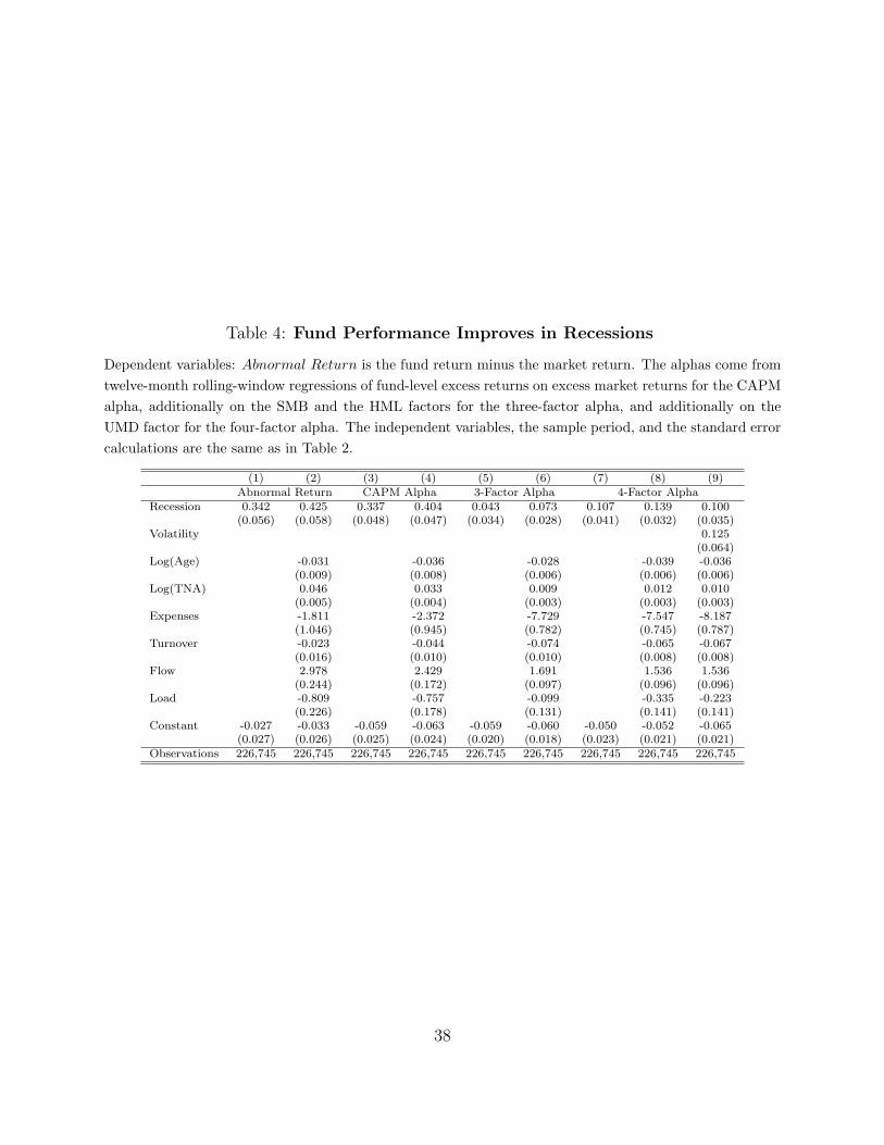
Table 4: Fund Performance Improves in Recessions
Dependent variables: Abnormal Return is the fund return minus the market return. The alphas come from
twelve-month rolling-window regressions of fund-level excess returns on excess market returns for the CAPM
alpha, additionally on the SMB and the HML factors for the three-factor alpha, and additionally on the
UMD factor for the four-factor alpha. The independent variables, the sample period, and the standard error
calculations are the same as in Table 2.
(1) (2) (3) (4) (5) (6) (7) (8) (9)Abnormal Return CAPM Alpha 3-Factor Alpha 4-Factor Alpha
Recession 0.342 0.425 0.337 0.404 0.043 0.073 0.107 0.139 0.100(0.056) (0.058) (0.048) (0.047) (0.034) (0.028) (0.041) (0.032) (0.035)
Volatility 0.125(0.064)
Log(Age) -0.031 -0.036 -0.028 -0.039 -0.036(0.009) (0.008) (0.006) (0.006) (0.006)
Log(TNA) 0.046 0.033 0.009 0.012 0.010(0.005) (0.004) (0.003) (0.003) (0.003)
Expenses -1.811 -2.372 -7.729 -7.547 -8.187(1.046) (0.945) (0.782) (0.745) (0.787)
Turnover -0.023 -0.044 -0.074 -0.065 -0.067(0.016) (0.010) (0.010) (0.008) (0.008)
Flow 2.978 2.429 1.691 1.536 1.536(0.244) (0.172) (0.097) (0.096) (0.096)
Load -0.809 -0.757 -0.099 -0.335 -0.223(0.226) (0.178) (0.131) (0.141) (0.141)
Constant -0.027 -0.033 -0.059 -0.063 -0.059 -0.060 -0.050 -0.052 -0.065(0.027) (0.026) (0.025) (0.024) (0.020) (0.018) (0.023) (0.021) (0.021)
Observations 226,745 226,745 226,745 226,745 226,745 226,745 226,745 226,745 226,745
38

Table 5: Robustness: Managers as the Unit of Observation
The dependent variables are fundamentals-based market-timing ability (Ftiming), fundamentals-based stock-picking ability (Fpicking), portfolio dispersion (Dispersion), and the four-factor alpha (4-Factor Alpha), allof which are tracked at the manager level. Columns with a ‘Y’ include manager fixed effects. The independentvariables, the sample period, and the standard error calculations are the same as in Table 2.
(1) (2) (3) (4) (5) (6) (7) (8)Ftiming Fpicking Dispersion 4-Factor Alpha
Recession 0.008 0.007 -0.701 -0.824 0.105 0.142 0.167 0.141(0.003) (0.002) (0.130) (0.132) (0.031) (0.024) (0.035) (0.035)
Log(Age) -0.002 -0.004 0.460 0.268 0.154 0.017 -0.032 -0.069(0.001) (0.001) (0.066) (0.065) (0.032) (0.021) (0.006) (0.008)
Log(TNA) -0.000 -0.000 -0.126 -0.139 -0.131 -0.093 0.007 0.003(0.000) (0.000) (0.032) (0.033) (0.018) (0.011) (0.004) (0.005)
Expenses 0.130 0.060 127.222 45.894 43.920 13.241 -8.225 -10.590(0.105) (0.146) (13.972) (13.867) (6.012) (4.504) (0.794) (1.138)
Turnover -0.005 -0.004 -0.287 0.210 -0.127 -0.014 -0.081 -0.035(0.002) (0.002) (0.077) (0.090) (0.030) (0.020) (0.010) (0.009)
Flow -0.009 -0.016 1.037 1.186 0.154 -0.374 1.832 1.483(0.009) (0.009) (0.613) (0.554) (0.121) (0.101) (0.097) (0.089)
Load -0.009 -0.069 -16.064 -5.832 -4.674 -0.231 -0.426 0.097(0.017) (0.023) (2.393) (2.307) (1.284) (0.809) (0.151) (0.172)
Fixed Effect N Y N Y N Y N YConstant -0.002 -0.002 2.966 2.977 1.438 1.447 -0.045 -0.043
(0.001) (0.001) (0.072) (0.068) (0.026) (0.008) (0.024) (0.021)Observations 332,676 332,676 249,942 249,942 332,776 332,776 332,776 332,776
39

A Appendix: Proofs of Propositions
A.1 Proof of Lemma 1
Proof. Following Admati (1985), we conjecture that the price vector p is linear in the payoff vector f and
the supply vector x: pr = A+Bf + Cx. We now verify that conjecture by imposing market clearing∫qjdj = x+ x (19)
Using (35) to substitute out the left hand side, and rearranging,
pr = −ρΣ(x+ x) + f + ΣΣ−1(µ− f)
Thus, the coefficients A, B, and C are given by
A = −ρΣx+ ΣΣ−1µ (20)
B = I − ΣΣ−1 (21)
C = −ρΣ (22)
which verifies our conjecture.
A.2 Mathematical Preliminaries
Matrices in terms of fundamental variances To determine the effect of changes in aggregate shock
variance on dispersion and profits, we need to express some of the matrices in terms of σ−1a . If we can
decompose the matrices into components that depend on σa and those that do not, we can differentiate the
expressions more easily.
First, we decompose the payoff precision matrices. To do this decomposition, we need to invert Σ. Doing
it by hand yields
Σ−1 =
σ−11 0 −b1σ−1
1
0 σ−12 −b2σ−1
2
−b1σ−11 −b2σ−1
2 σ−1a + b21σ
−11 + b22σ
−12
(23)
Similarly, the posterior precision matrix for investor j is
Σ−1j =
σ−11 0 −b1σ−1
1
0 σ−12 −b2σ−1
2
−b1σ−11 −b2σ−1
2 σa−1 + b21σ
−11 + b22σ
−12
(24)
40

It is useful to separate out the terms that depend on σa from those that do not. Define
S ≡
σ−11 0 −b1σ−1
1
0 σ−12 −b2σ−1
2
−b1σ−11 −b2σ−1
2 b21σ−11 + b22σ
−12
(25)
and let Sj be the posterior S, meaning that each σ1 is replaced with the posterior variance σ1j and each σ2
is replaced with the posterior variance σ2j .
Υa ≡
0 0 0
0 0 0
0 0 1
and Υ1 ≡
1 0 −b10 0 0
−b1 0 b21
(26)
so that ∂Σ−1j /∂σa
−1 = Υa and ∂Σ−1j /∂σ1
−1 = Υ1.
Then,
Σ−1 = S + σ−1a Υa (27)
Σ−1j = Sj + σa
−1j Υa (28)
Define the average posterior precision matrix when a fraction χ of investment managers have capacity to
be (Σ)−1 ≡∫jΣ−1j dj. Similarly, let Sa ≡
∫jSjdj and let Ka be the average amount of capacity that an
agent devotes to processing aggregate information. For example, if a fraction χ of investors are skilled, and
all skilled investors devote all their capacity K to processing aggregate information, Ka = χK. Recall that
σa−1j = σ−1
a +Kaj , then
(Σ)−1 = Sa + (σ−1a + Ka)Υa (29)
Useful matrices and expressions We derive several matrices and expressions that recur frequently in
the proofs below.
1) ∆ ≡ Σ−1j − (Σ)−1 = Σ−1
ηj − (Ση)−1: The difference between the precision of an informed manager’s
posterior beliefs and the precision of the average manager’s posterior beliefs is computed as:
Σ−1j − (Σ)−1 = Sj − Sa + (Kaj − Ka)Υa (30)
Now we show the equality. Bayes’ rule for variances of normal variables is Σ−1j = Σ−1 + Σ−1
ηj . Integrating
the left and right sides of this expression over managers j yields (Σ)−1 = Σ−1 + (Ση)−1. Subtracting one
expression from the other yields Σ−1j −(Σ)−1 = Σ−1
ηj −(Ση)−1. Therefore, ∆ ≡ Σ−1
j −(Σ)−1 = Σ−1ηj −(Ση)
−1.
Observe that ∆ is positive definite as long as the investor is more informed than the average: Kaj > Ka and
Kij > Ki for i ∈ {1, 2}.2) Σ: To compute the average variance we need to invert (Σ)−1. Replacing σa with (σ−1
a + Ka)−1 and
41

σi with (σ−1i + Ki)
−1, i ∈ {1, 2} in Eq. (24), and following the same inversion steps backwards, we get
Σ = (σ−1a + Ka)
−1bb′ +Φ, (31)
where b is the 3×1 vector of loadings of each asset on aggregate risk, and if K1 and K2 represent the average
amount of capacity devoted to processing information about assets 1 and 2,
Φ ≡
(σ−11 + K1)
−1 0 0
0 (σ−12 + K2)
−1 0
0 0 0
3) ΣΣ−1: Let σa ≡ (σ−1
a + Ka)−1, σ1 ≡ (σ−1
1 + K1)−1 and σ2 ≡ (σ−1
2 + K2)−1. Then we have the
following results:
ΣΣ−1 = (σabb′ +Φ)(S + σ−1
a Υa)
= σabb′S + σ−1
a ΦΥa + σaσ−1a bb′Υa +ΦS
=
σ1σ−11 0 b1(σaσ
−1a − σ1σ
−11 )
0 σ2σ−12 b2(σaσ
−1a − σ2σ
−12 )
0 0 σaσ−1a
(32)
where we have used that bb′S = 0, ΦΥa = 0, bb′Υa is a matrix of zeros except for the last column which
is equal to b and ΦS is equal to the first rows of S multiplied by σ1 and σ2 respectively. We have that
trace(ΣΣ−1) = σ1σ−11 + σ2σ
−12 + σaσ
−1a .
4) ΣΣ−1Σ:
ΣΣ−1Σ = (σaσ−1a bb′Υa +ΦS)(σabb
′ +Φ)
= σ2aσ
−1a bb′Υabb
′ + σaσ−1a bb′ΥaΦ+ σaΦSbb
′ +ΦSΦ
= σ2aσ
−1a bb′ + diag(σ2
1σ−11 , σ2
2σ−12 , 0)
=
σ2aσ
−1a b21 + σ2
1σ−11 σ2
aσ−1a b1b2 σ2
aσ−1a b1
σ2aσ
−1a b1b2 σ2
aσ−1a b22 + σ2
2σ−12 σ2
aσ−1a b2
σ2aσ
−1a b1 σ2
aσ−1a b2 σ2
aσ−1a
(33)
where we have used that bb′S = 0, ΦΥa = 0, bb′Υabb′ = bb′ and ΦSΦ is equal to the matrix described as a
diagonal above. We have that the trace(ΣΣ−1Σ) = σ2aσ
−1a [1 + b21 + b22] + σ2
1σ−11 + σ2
2σ−12 .
Signal about asset payoffs f It is convenient for the proofs below to express the signal as the true
asset payoff plus noise as follows: ηj = f + ϵj , where ϵj ∼ N (0, GΣejG′), Σej = diag{K−1
a ,K−11 ,K−1
2 }, and
G =
b1 1 0
b2 0 1
1 0 0
. Then the posterior precision is given by Σ−1j = Σ−1+Σ−1
ηj , where Σ−1ηj = Σ−1
ϵj = GΣejG′.
Note that Σ−1ηj and its inverse are positive definite as long as Ka,K1,K2 are strictly positive. We will assume
this throughout the proofs.
42

Average portfolio holdings The optimal portfolio for investor j is
qj =1
ρΣ−1j (µj − pr) (34)
This comes from the first order condition and is a standard expression in any portfolio problem with CARA
or mean-variance utility. Next, compute the portfolio of the average investor. Let the average of all investors’
posterior precision be (Σ)−1 ≡∫Σ−1j dj. Use the fact that µj = ΣjΣ
−1µ+ (I − ΣjΣ−1)ηj and the fact that
the signal noise is mean-zero to get that∫Σ−1j µjdj = Σ−1µ + ((Σ)−1 − Σ−1)f . This is true because the
mean of all investors’ signals are the true payoffs f and because the signal errors are uncorrelated with (but
of course, not independent of) signal precision.
q ≡∫qjdj =
1
ρ
(Σ−1µ+ ((Σ)−1 − Σ−1)f − (Σ)−1pr
)(35)
Using Bayes’ rule for the posterior variance of normal variables, we can rewrite this as
q ≡∫qjdj =
1
ρ
(Σ−1µ+ Σ−1
η f − (Σ)−1pr)
(36)
where Σ−1η ≡ Σ−1 − Σ−1 is the average investor’s signal precision.
Mean and variance of asset returns The vector of asset returns is (f − pr). Now replace pr with
A+Bf + Cx, where A, B, and C are given by Appendix A.1,
f − pr = (I −B)f −A− Cx (37)
Substituting in the coefficients in the pricing equation reveals that (I − B)µ − A = ρΣx, that I − B =
ΣΣ−1, and that C = −ρΣ, and therefore f − pr = Σ(Σ−1(f − µ) + ρx+ ρx). Since a linear combination of
two normal variables is also a normal variable, we can write
f − pr = w + V 1/2z where z ∼ N(0, I), (38)
V ≡ V ar[f − pr] = Σ(Σ−1 + ρ2σxI)Σ (39)
w ≡ E[f − pr] = ρΣx. (40)
A key partial derivative for evaluating comparative statics will be ∂V∂σa
. So, it is useful to evaluate that
here. Use (31) and (33) to write V as
V = σ2aσ
−1a bb′ + diag(σ2
1σ−11 , σ2
2σ−12 , 0) + ρ2σx[σabb
′ +Φ]2
When taking the partial derivative with respect to σa, we hold Ka fixed. Note that σ−1a − σ−1
a +Ka. Thus,
∂V/∂σa = σ2aσ
−2a [2σaσ
−1a − 1]bb′ + 2ρ2σxσ
2aσ
−2a Σbb′ (41)
Note that this is multiplied by σ2aσ
−2a > 0 throughout and post-multiplied by bb′, which is positive definite.
43

Since a product of positive definite matrices is positive definite, a sufficient condition for ∂V/∂σa positive
definite is
[2σaσ−1a − 1]I + 2ρ2σxΣ is positive definite. (42)
This is the condition under which the variance of expected returns increases when aggregate shock
variance increases. If 2σaσ−1a > 1, which implies that Ka < σ−1
a , this derivative will be positive. Since
the maximum possible average capacity devoted to the aggregate shock is the total capacity of informed
investors K times the fraction of informed investors, a sufficient condition for ∂V/∂σa to be positive definite
is that χK < σ−1a . Note also that the second term is a positive definite matrix. Suppose we do an
eigen-decomposition: Let Σ = ΓΛΓ′. Note that I = ΓIΓ′. Thus, the eigenvalue matrix of the sum in (42) is
[2σaσ−1a −1]I+2ρ2σxΛ. Since Σ is positive definite, all the entries of Λ are positive. Thus, if σx is sufficiently
large, the whole eigenvalue matrix will be positive and therefore, ∂V/∂σa will be positive definite. Thus a
second sufficient condition for (42) to hold is σx sufficiently large.
Portfolio dispersion Using the optimal portfolio expressions, (34) and (36), and Bayes’ rule (µj =
Σj(Σ−1µ+Σ−1
ηj ηj)), the difference in portfolios (qj − q) is
(qj − q) =1
ρ
[Σ−1ηj ηj − (Ση)
−1f + ((Σ)−1 − Σ−1j )pr
]where (Ση)
−1 ≡∫Σ−1ηj dj is the average manager’s signal precision.
Next, we need to take into account that signals and payoffs are correlated. To do this, replace the signal
ηj with the true payoff, plus signal noise: ηj = f + ϵj ,
(qj − q) =1
ρ
[Σ−1ηj ϵj + (Σ−1
ηj − (Ση)−1)f − (Σ−1
j − (Σ)−1)pr]
Recall that ∆ ≡ Σ−1j − (Σ)−1 = Σ−1
ηj − (Ση)−1. Substituting this in and combining terms yields
(qj − q) =1
ρ
[Σ−1ηj ej +∆(f − pr)
]Substituting (38) yields
(qj − q) =1
ρ
[Σ−1η ϵj +∆(V 1/2z + w)
](43)
To work out the expectation of this quantity squared, recognize that this is the square of a sum of one
constant and two, independent, mean-zero, normal variables. Since ϵj and x are independent, all the cross
terms drop out, leaving
E[(qj − q)′(qj − q)] =1
ρ2[Tr(Σ−1
ηj ) + Tr(∆V∆) + w′∆∆w] (44)
Expected portfolio return Let z ∼ N(0, I) and V ≡ Σ(Σ−1 + ρ2σxI)Σ as in the previous section, then
f − pr can be expressed as:
f − pr = ((I −B)f −A− Cx) = Σ(ρx+Σ−1(f − µ) + ρx) = w + V 1/2z
44

Recalling (43), the expected profits are given by:
E[(qj − q)′(f − pr)] =1
ρE[[Σ−1ηj ϵj +∆(V 1/2z + w)]′(V 1/2z + w)
]=
1
ρE[ϵ′jΣ
−1ηj w + ϵ′jΣ
−1ηj V
1/2z + (w′ + z′V 1/2)∆(V 1/2z + w)]
=1
ρE[ϵ′jΣ
−1ηj w + ϵ′jΣ
−1ηj V
1/2z + 2w′∆V 1/2z + w′∆w + z′V 1/2∆V 1/2z]
=1
ρE[w′∆w + z′V 1/2∆V 1/2z
]=
1
ρ
[ρ2x′Σ∆Σx+ Tr
(V 1/2∆V 1/2E(zz′)
)]=
1
ρ
[ρ2x′Σ∆Σx+ Tr(∆V )
]= ρTr(x′Σ∆Σx) +
1
ρTr(∆V ) (45)
where the fourth equality comes from the fact that ϵj and z are mean zero and uncorrelated.
Dispersion of portfolio returns Using results from the previous part, the dispersion in fund profits is
given by:
E[((qj − q)′(f − pr))2] = E
[(1
ρ[Σ−1η ej +∆V 1/2z +∆w]′(w + V 1/2z)
)2]
Using the fact that for any random variable x we have that V (x) = E(x2)−E2(x), the dispersion of funds’
portfolio returns is equal to:
E[((qj − q)′(f − pr))2] =1
ρ2E[(
[Σ−1ηj ej +∆V 1/2z +∆w]′(V 1/2z + w)
)2]=
1
ρ2V ar
([Σ−1ηj ej +∆V 1/2z +∆w]′(V 1/2z + w)
)+
1
ρ2
(E[Σ−1
ηj ej +∆V 1/2z +∆w]′(V 1/2z + w))2
We compute each term separately.
V ar(·) = V ar[e′jΣ
−1ηj w + e′jΣ
−1ηj V
1/2z + 2w′∆V 1/2z + w′∆w + z′V 1/2∆V 1/2z]
= V ar[e′jΣ
−1ηj w + e′jΣ
−1ηj V
1/2z + 2w′∆V 1/2z + w′∆w + z′V 1/2∆V 1/2z]
= w′Σ−1ηj w + 0 + 4w′∆V∆w + 0 + 2Tr(∆V∆V )
= ρ2Tr(x′Σ′Σ−1ηj Σx) + 4ρ2Tr(x′Σ′∆V∆Σx) + 2Tr(∆V∆V )
and
E(·)2 = (w′∆w)2 + Tr2(∆V ) + 2w′∆wTr(∆V )
= ρ4Tr2(x′Σ′∆Σx) + Tr2(∆V ) + 2ρ2Tr(x′Σ′∆Σx)Tr(∆V )
45

Substituting back we have:
E[((qj − q)′(f − pr))2] = Tr(x′Σ′Σ−1ηj Σx) + 4Tr(x′Σ′∆V∆Σx) +
2
ρ2Tr(∆V∆V )
+ ρ2Tr2(x′Σ′∆Σx) +1
ρ2Tr2(∆V ) + 2Tr(x′Σ′∆Σx)Tr(∆V ) (46)
Expected Utility From (9) in the main text, we know that expected utility is
U1j =1
2trace(Σ−1
j V ar[µj − pr]) +1
2E1[µj − pr]′Σ−1
j E1[µj − pr]
where we have normalized initial wealth W0 = 0. The excess return is given by:
µj − pr = Σj(Σ−1µ+Σ−1
ηj ηj)−A−Bf − Cx
The signal η can be expressed as the true asset payoff f , plus orthogonal signal noise ϵj .
µj − pr = ΣjΣ−1µ−A+ (ΣjΣ
−1ηj −B)f + ΣjΣ
−1ηj ϵj − Cx
Since µ and A are known constants and f , ϵj , and x are independent, with variances Σ, Σηj , and σxI
respectively, the variance term is given by:
V ar[µj − pr] = (ΣjΣ−1ηj −B)Σ(ΣjΣ
−1ηj −B)′ + ΣjΣ
−1ηj Σj + CC ′σx
Substituting in for the price coefficients using (20), (21), and (22) yields
V ar[µj − pr] = (Σ− Σj)Σ−1(Σ− Σj)
′ + ΣjΣ−1η Σj + ρ2σxΣΣ
Next, work out the second term by using the expression above for µj − pr and taking the expectation:
E[µj − pr] = ΣjΣ−1µ−A+(ΣjΣ
−1ηj −B)µ. Substituting in the coefficients A and B, and simplifying reveals
that E[µj − pr] = ρΣx. Thus,
E1[µj − pr]′Σ−1j E1[µj − pr] = ρ2x′ΣΣ−1
j Σx
Thus, expected utility is
U1j =1
2trace
(Σ−1j (Σ− Σj)Σ
−1(Σ− Σj)′ +Σ−1
ηj Σj + ρ2Σ−1j ΣΣσx
)+ρ2
2x′ΣΣ−1
j Σx
We can simplify the terms inside the trace to get the final expression which is convenient for the following
proofs:
U1j =1
2trace
(Σ−1j [Σ(ρ2σxI +Σ−1)Σ] + I − 2Σ−1Σ
)+ρ2
2x′ΣΣ−1
j Σx (47)
or equivalently
U1j =1
2trace
(Σ−1j V + I − 2Σ−1Σ
)+ρ2
2x′ΣΣ−1
j Σx (48)
46

A.3 Lemma 2: Investors Prefer Not To Learn Price Information
The idea behind this result is that an investor who learns from price information, will infer that the asset is
valuable when its price is high and infer that the asset is less valuable when its price is low. Buying high and
selling low is generally not a way to earn high profits. This effect shows up as a positive correlation between
µ and pr, which reduces the variance V ar[µj − pr].
Mathematical Preliminaries: Note that B−1(pr − A) = f + B−1Cx. Since x is a mean-zero shock, this
is an unbiased signal about the true asset payoff f . The precision of this signal is Σ−1p ≡ σ−1
x B′(CC ′)−1B.
Lemma 2. A manager who could choose either learning from prices and observing a signal η|f ∼ N(f, Ση)
or not learning from prices and instead getting a higher-precision signal η|f ∼ N(f,Ση), where the signals
are conditionally independent across agents, and where Σ−1η = Σ−1
p + Σ−1η , would prefer not to learn from
prices.
Proof. From (9) in the main text, we know that expected utility is
U1j =1
2trace(Σ−1
j V ar[µj − pr]) +1
2E1[µj − pr]′Σ−1
j E1[µj − pr]
By Bayes’ rule, the two options yield equally informative posterior beliefs: Σ−1j = Σ−1+Σ−1
η = Σ−1+Σ−1p +
Σ−1η . Likewise, since both possibilities give the manager unbiased signals, beliefs are a martingale, meaning
that E1[µj − pr], is identical under the two options.
Thus, the only term in expected utility that is affected by the decision to learn information from prices
is V ar[µj − pr]. Let µj = E[f |η] be the posterior expected value of payoffs for the manager who learns from
the conditionally independent signal and µ = E[f |p, η] the posterior expected value for the manager that
chooses to learn information in prices.
From properties of the variance we have that:
V ar[µj − pr]− V ar[µ− pr] = V ar[µj ]− V ar[µ] + 2(Cov[µ, pr]− Cov[µj , pr])
Step 1: show that the first two terms are equal and thus cancel out. By Bayes’ law: µj = Σj(Σ−1µ+Σ−1
ηj η).
Writing the signal as η = f + ϵ (see Preliminaries) we have:
µj = Σj(Σ−1µ+Σ−1
ηj f +Σ−1ηj ϵ)
Then V ar[µj ] = ΣjΣ−1ηj (ΣΣ
−1ηj + I)Σj .
Again, by Bayes’ law, µ = Σj(Σ−1µ+Σ−1
p B−1(pr −A) + Σ−1η η). Write the signal as η = f + ϵ and use
the price equation pr = A+Bf + Cx we get:
µ = Σj(Σ−1µ+Σ−1
p B−1(Bf + Cx) + Σ−1η (f + ϵ))
= Σj(Σ−1µ+ (Σ−1
p + Σ−1η )f +Σ−1
p B−1Cx+ Σ−1η ϵ)
= Σj(Σ−1µ+Σ−1
η f +Σ−1p B−1Cx+ Σ−1
η ϵ)
where the last equality comes from the assumption that Σ−1η +Σ−1
p = Σ−1η .
47

Then taking variance:
V ar[µ] = Σj(Σ−1η ΣΣ−1
η + σxΣ−1p B−1CC ′B−1Σ−1
p + Σ−1η ])Σj
= ΣjΣ−1η (ΣΣ−1
η + I)Σj + σxΣj(Σ−1p B−1CC ′B−1Σ−1
p − Σ−1p )Σj
= ΣjΣ−1η (ΣΣ−1
η + I)Σj + ΣjΣ−1p (σxB
−1CC ′B−1Σ−1p − I)Σj
= ΣjΣ−1η (ΣΣ−1
η + I)Σj
where the last term cancels because Σ−1p ≡ σ−1
x B′(CC ′)−1B. Therefore, V ar[µj ] = V ar[µ].
Step 2: Show that Cov[µ, pr] > Cov[µj , pr]. Now we compute the covariance terms, using the fact that
adding constant terms do not change change the value of the covariance.
Cov[µj , pr] = Cov[µj − Σj(Σ−1ηj +Σ−1)µ, pr −A]
= Cov[ΣjΣ−1ηj (f − µ) + ΣjΣ
−1ηj ϵ, B(f − µ) + Cx]
= Cov[ΣjΣ−1ηj (f − µ), B(f − µ)]
= E[ΣjΣ−1ηj (f − µ)(f − µ)′B′]
= ΣjΣ−1ηj ΣB
′
Cov[µ, pr] = Cov[µ− Σj(Σ−1η +Σ−1)µ, pr −A]
= Cov[ΣjΣ−1ηj (f − µ) + ΣjΣ
−1p B−1Cx+ ΣjΣ
−1η ϵ, B(f − µ) + Cx]
= Cov[ΣjΣ−1ηj (f − µ), B(f − µ)] + Cov[ΣjΣ
−1p B−1Cx,Cx]
= ΣjΣ−1ηj ΣB
′ + E[ΣjΣ−1p B−1Cxx′C ′]
= ΣjΣ−1ηj ΣB
′ + ΣjΣ−1p (σ−1
x B′(CC ′)−1B)−1B′
= Cov[µj , pr] + ΣjB′
In summary, we have shown that V ar[µj − pr]−V ar[µ− pr] > 0. The difference in utility from learning
conditionally independent information and learning price information is given by
1
2trace(Σ−1
j (V ar[µj − pr]− [V ar[µ− pr]))
Since the expression inside the trace is a product of positive definite matrices, the difference in expected
utilities is positive.
48

A.4 Proof of Proposition 1
If (42) holds, then the marginal value of a given investor j reallocating an increment of capacity from stock-
specific shock i ϵ {1, 2} to the aggregate shock is increasing in the aggregate shock variance σa: If Kaj = K
and Kij = K − K, then ∂2U/∂K∂σa > 0.
Proof. We want to take a cross-partial derivative of utility with respect to σa and K. To do this, we will
substitute out the Σ−1j terms using (27), (28), and (29). Then, we will use the fact that, by the chain rule,
∂U/∂K = ∂U/∂Kaj − ∂U/∂Kij . Therefore,
∂2U/∂K∂σa = ∂2U/∂Kaj∂σa − ∂2U/∂Kij∂σa
We consider each of these two cross-partial derivatives separately in cases a and b.
Part a: The marginal value of a given investor j having additional capacity Kaj devoted to learning about
the aggregate shock a is increasing in the aggregate shock variance: ∂2U/∂Kaj∂σa > 0.
Recall the expression for utility in (47):
U1j =1
2trace
(Σ−1j [Σ(ρ2σxI +Σ−1)Σ] + I − 2Σ−1Σ
)+ρ2
2x′ΣΣ−1
j Σx
Sign last term: ρ2
2 x′ΣΣ−1
j Σx
Note that Kaj appears only in Σ−1j . Recall that ∂Σ−1
j /∂σa−1 = Υa. Since σa
−1 = σa−1 + Kaj , the
chain rule implies that ∂Σ−1j /∂Kaj = Υa. Thus, the last term has Kaj derivative (ρ
2/2)x′ΣΥaΣx. The only
term in this expression that varies in σa is Σ. Since Σ has every entry increasing in σa (equation 31), and Σ
and Υa are positive semi-definite matrices, this term has a positive cross-partial derivative ∂2/∂Kj∂σa > 0.
One can also compute it analytically and obtain: ρ2
σ2a(σ
−1a +Ka)2
ΥaΣxx′ > 0. Thus, a sufficient condition for
∂2U/∂Kj∂σa > 0 is for the trace term to have a positive cross partial derivative.
Sign trace: trace(Σ−1j [Σ(ρ2σxI +Σ−1)Σ] + I − 2Σ−1Σ
)Observe that only the first element of the trace depends on Kaj and exclusively through Σ−1
j . We take
derivative of the trace with respect to Kaj to get:
trace(ΥaΣ(ρ2σxI +Σ−1)Σ)
Note from equation (39) that Σ(ρ2σxI + Σ−1)Σ = V . We know that the derivative of V with respect
to σa is positive if condition (42) holds. Since upa is invariant in σa and is positive semidefinite, the partial
derivative of the product is positive semidefinite, and therefore the trace is ≥ 0 if (42) holds. Thus, (42) is
a sufficient condition for the cross-partial to be positive.
Part b: The marginal value of a given investor j having additional capacity Kij devoted to learning about
stock-specific shock i is constant in the aggregate shock variance: ∂2U/∂Kij∂σa = 0.
49

Proof. Without loss of generality, we consider reallocating capacity from the asset 1 shock to the aggregate
shock (i = 1). The same proof follows if it were asset 2 instead.
Sign last term: ρ2
2 x′ΣΣ−1
j Σx.
Note that K1j appears only in Σ−1j . Recall that ∂Σ−1
j /∂σ1−1 = Υ1. Since σ1
−1 = σ1−1 +K1j , using the
chain rule, we get ∂Σ−1j /∂K1j = Υ1. Therefore, ∂/∂K1j(x
′ΣΣ−1j Σx) = x′ΣΥ1Σx.
Because of the structure of the Υ1 matrix, it turns out that using (26) and (31) to multiply out the three
matrices ΣΥ1Σ delivers
ΣΥ1Σ =
(σ−11 + K1)
−2 0 0
0 0 0
0 0 0
. (49)
Since this has no σa term in it and both x and ρ are exogenous, the cross-partial derivative ∂2/∂K1j∂σa of
the last terms is zero.
Sign trace: trace(Σ−1j [Σ(ρ2σxI +Σ−1)Σ] + I − 2Σ−1Σ
)Observe that only the first element of the trace depends on K1j and exclusively through Σ−1
j . We take
derivative of the trace with respect to K1j to get:
trace(Υ1Σ(ρ2σxI +Σ−1)Σ)
From the multiplication above, we have that trace(ΣΥ1Σ) = (σ−11 + K1)
−2. Also, the sparse form of Υ1
causes the matrix multiplication of Υ1ΣΣ−1Σ′ to turn out neatly. Using (23), (26) and (31) to multiply out
the four matrices delivers
Υ1ΣΣ−1Σ′ =
σ−11 (σ−1
1 + K1)−2 0 0
0 0 0
−b1σ−11 (σ−1
1 + K1)−2 0 0
. (50)
The trace of this matrix is σ−11 (σ−1
1 +K1)−2. With these facts, the expression for ∂/∂Kij can be rewritten as:
(σ−11 + K1)
2(σ−11 + ρσx). Since this expression has no σa term in it, the cross-partial derivative ∂2/∂K1j∂σa
is zero.
In conclusion, if Ka ≤ σ−1a then ∂2U/∂Kaj∂σa > 0 and ∂2U/∂Kij∂σa = 0 and the difference of the
two terms is positive. Thus, if the average attention allocated to the aggregate shock is not too high, the
marginal value of a given investor j reallocating an increment of capacity from shock 1 to the aggregate
shock is increasing in the aggregate shock variance: ∂2U/∂K∂σa = ∂2U/∂Kaj∂σa − ∂2U/∂Kij∂σa > 0.
A.5 Proof of Proposition 2
If the size of the composite asset x3 is sufficiently large, then an increase in risk aversion increases the
marginal utility of reallocating a unit of capacity from the idiosyncratic shock to the aggregate shock:
∂/∂ρ(∂U/∂(Kaj −K1j) > 0.
50

Proof. We can rewrite ∂/∂ρ(∂U/∂(σ−1aj − σ−1
1j )) as ∂2U/∂ρ∂σ−1
aj − ∂2U/∂ρ∂σ−11j > 0.
We will work out each of these two terms separately. But first, both depend on the partial derivative of
utility with respect to risk aversion. Taking the partial derivative of utility in (47) with respect to ρ yields
∂U
∂ρ= ρσxTr[Σ
−1j ΣΣ] + x′ΣΣ−1
j Σx. (51)
The next step is to differentiate (51) with respect to σ−1aj . Since σ−1
aj is the precision of agent j’s
information, it does not affect aggregate variables such as Σ. Recalling that ∂Σ−1j /∂σ−1
aj = Υa,
∂2U
∂ρ∂σ−1aj
= ρσxTr[ΥaΣΣ] + x′ΣΥaΣx. (52)
Next, we follow the same steps to differentiate (51) with respect to σ−11j , which also affects only Σj .
Recalling that ∂Σ−1j /∂σ−1
1j = Υ1, and using the fact that the trace is invariant to matrix ordering,
∂2U
∂ρ∂σ−11j
= ρσxTr[ΣΥ1Σ] + x′ΣΥ1Σx. (53)
The extent to which risk aversion affects the utility of reallocating precision from risk 1 to risk a is the
difference of (52) and (53):
∂/∂ρ(∂U/∂(σ−1aj − σ−1
1j )) = ρσxTr[Σ(Υa −Υ1)Σ] + x′Σ(Υa −Υ1)Σx. (54)
If b1 < 1, then Υa − Υ1 =
−1 0 b1
0 0 0
b1 0 1− b21
is positive definite. Since Σ is positive definite, both the
trade and the second term will be positive and we have the result.
We can derive a different sufficient condition as follows. Multiplying out term-by-term ΣΥaΣ reveals
that it equals σ2abb
′. Multiplying out ΣΥ1Σ reveals that it equals
ΣΥ1Σ =
σ21 0 0
0 0 0
0 0 0
Thus,
Tr[Σ(Υa −Υ1)Σ] = σ2a(b
21 + b22 + 1)− σ2
1
and
x′Σ(Υa −Υ1)Σx = σ2a(b1x1 + b2x2 + x3)
2 − x21σ21
If these two terms are positive, then ∂/∂ρ(∂U/∂(σ−1aj − σ−1
1j )) > 0.
Note that the whole second partial derivative is increasing in x3, the supply of the composite asset:
∂/∂ρ(∂U/∂(σ−1aj − σ−1
1j )) = ρσx(σ2a(b
21 + b22 + 1)− σ2
1) + σ2a(b1x1 + b2x2 + xc)
2 − x21σ21 (55)
51

Thus, as long as the composite asset, meant to represent the entire market capitalization, aside from the
two assets 1 and 2, is large enough relative to assets 1 and 2, the cross-partial derivative will be positive.
A.6 Proof of Proposition 3
If (42) holds, then for given precisions of an investor j who is more informed than the average (i.e. for
fixed Kaj > Ka and Kij > Ki for i ∈ {1, 2}), an increase in aggregate risk σa: a) increases the dispersion
of fund portfolios E[(qj − q)′(qj − q)] where q ≡∫qjdj and b) increases the dispersion of funds’ portfolio
returns E[((qj − q)′(f − pr))2].
Proof of Part a):
Proof. From equation (44) in the preliminaries, we know that portfolio dispersion is given by:
E[(qj − q)′(qj − q)] =1
ρ2Tr(∆V∆) + Tr(x′∆ΣΣ∆x)
Now we take partial derivatives with respect to σa.
Term 1: The first term depends only on information choice variables. So, holding choices fixed, the
partial derivative with respect to σa is zero.
Term 2: Recall that ∆ ≡ Σ−1j −(Σ)−1 depends only on information choices, which we hold fixed, and thus
∂Tr(∆V∆)/∂σa = Tr(∆[∂V/∂σa
]∆). Furthermore, if the posterior precision of the investor is higher than
the average, ∆ is positive definite too. From the preliminaries we know that ∂V/∂σa is positive semi-definite
if condition (42) holds. Therefore, (42) is a sufficient condition for the second term to be positive.
Term 3: The derivative of term 3 with respect to σa is: Tr(x′∆[∂(ΣΣ)/∂σa
]∆x). This will be positive
if[∂(ΣΣ)/∂σa
]is positive semi-definite. We have that ΣΣ = (σ−1
a + Ka)−2bb′bb′ +2(σ−1
a + Ka)−1bb′Φ+Φ2
and thus the derivative with respect to σa is: 2σ−2a (σ−1
a + Ka)−3bb′bb′ + 2σ−2
a (σ−1a + Ka)
−2bb′Φ > 0.
In sum, all four terms in the expression for dispersion are increasing in σa.
Proof of Part b):
Proof. From equation (46) in the preliminaries, we know that dispersion of portfolio returns is given by:
E[((qj − q)′(f − pr))2] = Tr(x′Σ′Σ−1ηj Σx) + ρ2Tr2(x′Σ′∆Σx) + 4Tr(x′Σ′∆V∆Σx)
+2
ρ2Tr(∆V∆V ) +
1
ρ2Tr2(∆V ) + 2Tr(x′Σ′∆Σx)Tr(∆V )
Observe that Σ−1ηj and ∆ depend only on choice variables, which we hold fixed. Also, every entry of Σ
is increasing in σa. If condition (42) holds, ∂V/∂σa is a positive semi-definite matrix, which guarantees that
the whole expression is increasing in σa.
52

A.7 Proposition 4
If σx is sufficiently high, then for given Kaj ,Kij ∀j , an increase in risk aversion ρ increases the dispersion
of funds’ portfolio returns E[((qj − q)′(f − pr))2].
Proof. From equation (46) in the preliminaries, we have that the dispersion of portfolio returns is given by:
E[((qj − q)′(f − pr))2] = Tr(x′Σ′Σ−1ηj Σx) + 4Tr(x′Σ′∆V∆Σx) +
2
ρ2Tr(∆V∆V )
+ ρ2Tr2(x′Σ′∆Σx) +1
ρ2Tr2(∆V ) + 2Tr(x′Σ′∆Σx)Tr(∆V )
Taking derivatives with respect to ρ we get:
∂E[((qj − q)′(f − pr))2]
∂ρ= 4Tr(x′Σ′∆
∂V
∂ρ∆Σx) +
2
ρ2Tr
(∂(∆V∆V )
∂ρ
)− 4
ρ3Tr(∆V∆V )
+ 2ρTr2(x′Σ′∆Σx) +2
ρ2Tr(∆V )Tr
(∆∂V
∂ρ
)− 2
ρ3Tr2(∆V )
+ 2Tr(x′Σ′∆Σx)Tr(∆∂V
∂ρ
)Substitute (39) for V , ∂V∂ρ = 2ρσxΣΣ and ∂(∆V∆V )
∂ρ = 4ρσx∆ΣΣ−1Σ∆ΣΣ + 4ρ3σ2x∆ΣΣ∆ΣΣ:
= 8ρσxTr(x′Σ′∆ΣΣ∆Σx)︸ ︷︷ ︸>0
+2ρTr2(x′Σ′∆Σx)︸ ︷︷ ︸>0
+4ρσxTr(x′Σ′∆Σx)Tr
(∆ΣΣ
)︸ ︷︷ ︸
>0
+ Tr(∆ΣΣ
[4ρσ2
x∆Σ− 4
ρ3Σ−1∆Σ−1
]ΣΣ
)︸ ︷︷ ︸
I
+ 2ρσ2xTr
2(∆ΣΣ)− 2
ρ3Tr2(∆ΣΣ−1Σ)︸ ︷︷ ︸
II
We need a condition such that I and II are positive and thus the derivative will be positive. For (I),
we need 4ρσ2x∆Σ ≥ 4
ρ3Σ−1∆Σ−1, or
Tr(∆Σ(ρ4σ2xI −∆−1Σ−1Σ−1∆Σ−1)) ≥ 0. (56)
For (II), we need 2ρσ2xTr
2(∆ΣΣ) ≥ 2ρ3Tr
2(∆ΣΣ−1Σ), or
Tr(∆Σ(ρ2σxI − Σ−1)Σ) ≥ 0. (57)
In both cases, if σx is sufficiently high, the conditions are met.
A.8 Proof of Proposition 5
If (42) holds, then an increase in aggregate shock variance increases the difference between an informed
investor expected certainty equivalent return and the expected certainty equivalent return of an uninformed
53

investor: ∂(Uj − UU )/∂σa > 0.
Proof. From (48) we know that time-1 expected utility for an agent who has posterior belief precision Σ−1j
is given by
U1j =1
2trace
(Σ−1j V + I − 2Σ−1Σ
)+ρ2
2x′ΣΣ−1
j Σx
Since the result is about the difference in utility between an informed and an uninformed agent, who
has posterior belief precision Σj = Σ, we take the difference of these two expected utilities:
Uj − UU =1
2trace
([Σ−1j − Σ−1]V
)+ρ2
2x′Σ[Σ−1
j − Σ−1]Σx
Recall that Σ−1j − Σ−1 = Σ−1
ηj , then:
Uj − UU =1
2trace
(Σ−1ηj V
)+ρ2
2x′ΣΣ−1
ηj Σx
Since Σ−1ηj is a choice variable it does not change in σa. Therefore we have that the partial derivative of
the utility difference with respect to σa is:
∂(Uj − UU )
∂σa=
1
2trace
(Σ−1ηj
[∂V
∂σa
])+ ρ2trace
(x′Σ−1
ηj
[∂Σ
∂σa
]Σx
)Differentiating (31) tells us that ∂Σ/∂σa is a positive scalar times bb′, which is positive semi-definite.
If (42) holds, then ∂V/∂σa is also positive semi-definite. Therefore, both trace terms are positive and
∂(Uj − UU )/∂σa > 0.
A.9 Proof of Corollary 1
If (42) holds, then for given precisions of an investor j who is more informed than the average (i.e. for
fixed Kaj > Ka and Kij > Ki for i ∈ {1, 2} strictly positive), an increase in aggregate risk σa increases the
expected profit of an informed fund, E[(qj − q)′(f − pr)], where q ≡∫qjdj.
Proof. From (45), the expected profits are given by:
E[(qj − q)′(f − pr)] = ρTr(x′Σ∆Σx) +1
ρTr(∆V )
Then∂E[(qj − q)′(f − pr)]
∂σa= 2ρTr
(x′∆
[∂Σ
∂σa
]Σx
)+
1
ρTr
(∆
[∂V
∂σa
])> 0
since ∆ = Σ−1ηj − (Ση)
−1 does not depend on σa and both Σ and V are increasing in σa as long as condition
(42) holds. The requirement that the investor is more informed than the average ensures that ∆ is positive
semi-definite.
54

A.10 Proposition 6
For given Kaj ,K1j ,K2j strictly positive, an increase in risk aversion ρ for all investors increases the
difference in expected certainty equivalent returns between an informed and an uninformed investor: ∂(Uj −UU )/∂ρ > 0.
Proof. From the proof of proposition (5) we have that the difference in expected utilities between an informed
investor and an uninformed investors is:
Uj − UU =1
2Tr(Σ−1
j (Σ− Σj)Σ−1(Σ− Σj)
′)− 1
2Tr
(Σ−1(Σ− Σ)Σ−1(Σ− Σ)′
)+1
2Tr(Σ−1
ηj Σj) +ρ2
2
{σxTr(ΣΣ
−1ηj Σ) + x′ΣΣ−1
ηj Σx}
where Σ−1ηj = Σ−1
j − Σ−1. Differentiating with respect to ρ yields:
∂(Uj − UU )
∂ρ= ρ
{σxTr(ΣΣ
−1ηj Σ) + x′ΣΣ−1
ηj Σx}
As long as Kaj ,Kij are strictly positive, then Σηj and its inverse will be a positive definite matrices. Since
Σ is clearly positive definite, we obtain the desired result.
55
Related Documents