Rating Through-the-Cycle: What does the Concept Imply for ...Concept Imply for Rating Stability and Accuracy? Prepared by . John Kiff †, Michael Kisser ‡ and Liliana Schumacher

Rating Through-the-Cycle: What does the

Concept Imply for Rating Stability and

Accuracy?

John Kiff, Michael Kisser and Liliana Schumacher

WP/13/64

© 2013 International Monetary Fund WP/13/64

IMF Working Paper

Monetary and Capital Markets

Rating Through-the-Cycle: What does the

Concept Imply for Rating Stability and Accuracy?

Prepared by John Kiff†, Michael Kisser

‡ and Liliana Schumacher

†

Authorized for distribution by Laura Kodres

March 2013

Abstract

Credit rating agencies face a difficult trade-off between delivering both accurate and stable

ratings. In particular, its users have consistently expressed a preference for rating stability,

driven by the transactions costs induced by trading when ratings change frequently. Rating

agencies generally assign ratings on a through-the-cycle basis whereas banks' internal

valuations are often based on a point-in-time performance, that is they are related to the

current value of the rated entity's or instrument's underlying assets. This paper compares the

two approaches and assesses their impact on rating stability and accuracy. We find that while

through-the-cycle ratings are initially more stable, they are prone to rating cliff effects and

also suffer from inferior performance in predicting future defaults. This is because they are

typically smooth and delay rating changes. Using a through-the-crisis methodology that uses a

more stringent stress test goes halfway toward mitigating cliff effects, but is still prone to

discretionary rating change delays.

JEL Classification Numbers: G20, G24, G28

Keywords: Credit ratings; Credit rating agencies; Credit rating migration

We thank Laura Kodres for the valuable feedback.

† International Monetary Fund Author’s, e-mail Address: [email protected], and [email protected]

‡ Norwegian School of Economics Author, e-mail Address: [email protected]

This Working Paper should not be reported as representing the views of the IMF.

The views expressed in this Working Paper are those of the author(s) and do not necessarily

represent those of the IMF or IMF policy. Working Papers describe research in progress by the

author(s) and are published to elicit comments and to further debate.

Contents Page

I Introduction . . . . . . . . . . . . . . . . . . . . . . . . . . . . . . . . . . . 3

II Literature Overview . . . . . . . . . . . . . . . . . . . . . . . . . . . . . . 4

IIIThe Model . . . . . . . . . . . . . . . . . . . . . . . . . . . . . . . . . . . . 6

IV Numerical Analysis . . . . . . . . . . . . . . . . . . . . . . . . . . . . . . 11

A Stability of Ratings . . . . . . . . . . . . . . . . . . . . . . . . . . . . . 15

B Predictive Power of Ratings . . . . . . . . . . . . . . . . . . . . . . . . 19

V Summary . . . . . . . . . . . . . . . . . . . . . . . . . . . . . . . . . . . . 21

VI Appendix . . . . . . . . . . . . . . . . . . . . . . . . . . . . . . . . . . . . 26

A Derivation of Worst Case Scenario . . . . . . . . . . . . . . . . . . . . . 26

B Rating Mapping . . . . . . . . . . . . . . . . . . . . . . . . . . . . . . . 28

2

3

I Introduction

Credit Rating Agencies (CRAs) face a difficult tradeoff between accuracy and stabil-

ity when assigning credit ratings. On one hand, their ratings should provide the most

accurate estimate of the corresponding default risk of the underlying asset while on the

other hand, users prefer that they do not change too frequently, see Cantor and Mann

(2006). This is due to the fact that credit ratings are often used in fixed income port-

folio composition and collateral acceptability guidelines, in bond covenants and other

financial contracts, and various financial rules and regulations.

On a conceptual level, CRAs can assign ratings on either a Point in Time (PIT) or a

Through the Cycle (TTC) basis. Loosely speaking, the PIT approach can be thought of

as using current information when computing the default risk metrics that are mapped

into ratings. Credit ratings assigned under the PIT approach should provide the most

accurate estimate of future default probabilities and expected losses. On the other hand,

the TTC approach is supposed to balance the need for accurate default estimates and

the desire to achieve rating stability.

This paper investigates the stability and accuracy of credit ratings within a stochastic

framework. Specifically, we first employ contingent claims analysis to simulate asset

values which are subject to both transitory and cyclical shocks. Credit ratings are then

assigned based on expected asset values and underlying asset volatility and, in case of

the TTC approach, on an additional stress test. The paper then compares assigned

credit ratings under the TTC and PIT approaches and assesses the impact on rating

stability and accuracy.

4

Section (II) provides a brief summary of the academic literature and evidence from

CRAs in order to define the actual meaning of through the cycle rating. Section (III)

presents a simple structural credit risk model and explains how asset values are mapped

into credit ratings under both rating approaches. Section (IV) presents the main anal-

ysis and Section (V) concludes.

II Literature Overview

While anecdotal evidence from CRAs confirms their use of the TTC approach, it turns

out that there is no single and simple definition of what TTC rating actually means.

We will therefore provide a short summary of both academic research and evidence

from CRAs themselves before defining the meaning of TTC rating used in this paper.

Altman and Rijken (2006) investigate the conflicts of interests arising from the CRA’s

often competing objectives of providing ratings that are timely, stable, and accurate

predictors of defaults. Using credit scoring models, they show that CRAs focus on

the permanent credit risk component when assigning ratings. Besides, they argue that

CRAs are slow in adjusting their ratings and that the slow reaction is the most im-

portant source of rating stability. Therefore, in their view TTC approaches capture a

trend component.

In two different papers, Loeffler (2004, 2005) investigates the rating impact of the

TTC approach and the rating change smoothing that CRAs use to slow the rating

adjustment process. Building on a model initially proposed by Fama and French (1988)

on the effect of permanent and transitory components on stock prices, Loeffler (2004)

5

assumes that the market value of an asset consists of both a permanent and a cyclical

component. In order to assign credit ratings according to the TTC approach, he imposes

a stress scenario on the cyclical component when forecasting future asset values. In

this view, a TTC rating is conditional on using stressed cyclical fluctuations. In a

different paper, Loeffler (2005) investigates the CRAs’ slow reaction to deteriorating

credit quality and argues that the slow reaction can be explained by the desire to avoid

subsequent rating reversals. Topp and Perl (2010) investigate actual corporate ratings

assigned by Standard and Poor’s and show that even though the CRAs claim to only

focus on the permanent risk component, actual ratings reveal cyclical patterns. Finally,

Carey and Hrycay (2001) argue that the TTC rating approach actually used by CRAs

entails estimating default risk over a long horizon and that additionally the estimate is

subject to an explicit stress scenario.

The academic literature is consistent with evidence from the CRAs themselves. In a

special comment to Moody’s rating users, Cantor and Mann (2006) analyze the tradeoff

between ratings accuracy and stability and argue that CRAs desire to deliver both

accurate and stable ratings. Also, Standard and Poor’s claim that “when assigning

and monitoring ratings, we consider whether we believe an issuer or security has a

high likelihood of experiencing unusually large adverse changes in credit quality under

conditions of moderate stress. In such cases, we would assign the issuer a lower rating

than we would have otherwise.” For more details see Adelson et al. (2010). Further

examples relating to the agencies’ practices can be found in Cantor and Mann (2003).

We combine the approaches described above and define the TTC approach as a two

step process. Ratings are assumed to have a permanent and cyclical component and

6

ex-ante, they are calculated conditional on a stress scenario for the cyclical component.

Ex-post, ratings are filtered and not adjusted immediately. A formal definition will

follow after we have introduced the model in the next section.

III The Model

The structural credit risk model presented in this section builds on Loeffler (2004) and

subsequent extensions and modifications to it. To investigate the effect of the different

rating approaches it is assumed that the asset value of a firm or sovereign consists of

both a permanent and a cyclical component, i.e.

xt = x∗t + yt (1)

where xt denotes the logarithm of the observed asset value, x∗t the permanent (funda-

mental) value and yt captures the cyclical component. It is further assumed that x∗t

follows a random walk with drift, so that

dx∗ = µdt+ σdW (2)

where µ is the drift rate, σ the volatility and Wt is a standard Wiener process. Note

that dW = ε√dt where ε v N(0, 1) and dt denotes the length of the time step. In order

to introduce cyclicality, yt follows an autoregressive process of order one, i.e.

7

yt = ρyt−1 + ut (3)

where 0 < ρ < 1, ut v N(0, σ2u) and Cov(εt, ut) = 0.

The effect of the chosen credit rating approach is analyzed by computing default

probabilities under both rating approaches and then mapping those into discrete ratings

using Moody’s idealized default probabilities.1 As a first step, we observe that the

expected value of the permanent and cyclical value components for any final time T is

given by

E(x∗T ) = x∗t

E(yT ) = ρTyt

E(xT ) = x∗t + ρTyt (4)

where t < T . In the Contingent Claims Analysis framework, a default occurs when

the value of an entity’s assets falls through a distress threshold which is related to its

liabilities.2 Prior to default, default risk is measured in terms of distance to default -

the number of standard deviations the asset value has to drop before it hits the distress

1These idealized default probabilities were designed solely for use on structured products, andsimilar ones were used by Fitch and Standard and Poor’s for the same purpose. However, they do revealthe CRA target default probabilities, even if they are not actually used to rate other credits. Idealizeddefault rates are based on historical default rates over various horizons, and analyst judgements. Theidealization process is intended to ensure the appropriate smooth ranking of default probabilities byrating.

2In the case of a sovereign, assets include foreign reserves and fiscal assets such as the presentvalue of taxes and other revenues, and liabilities include base money, public debt (local and foreigncurrency), and guarantees (explicit and implicit). See Gray et al. (2007).

8

threshold. The larger the distance to default, the smaller is the probability of default.3

Assuming a forecasting horizon of s periods, one can immediately compute the distance

to default measure under the PIT methodology, i.e.

DDPIT =E(xt+s)− d

σ(x)(5)

where d is the face value of the liabilities and σ(x) is the volatility of the observed

value xt.4 In order to compute risk metrics under the TTC approach, we need a formal

definition of what the through the cycle concept actually means.

Definition 1 TTC rating is defined as a two step process. Ex-ante ratings are calcu-

lated conditional on a stress scenario for the cyclical component. Ex-post rating changes

are smoothed and thus not adjusted immediately.

To incorporate the intuition of definition 1 into our framework, we follow Loeffler (2004)

and Carey and Hrycay (2001) who argue that the worst case scenario is based on an

estimate of the borrower’s default probability in a stress scenario, i.e.

p(D) = p(D|S)p(S) (6)

where p(D) is the unconditional default probability, p(D|S) is the probability of default

in the stress scenario and p(S) is the probability of the stress scenario. We then calculate

the prediction interval of a v-period forecast for an autoregressive process and obtain

3See Gray et al. (2007)4Following Loeffler (2004), the unconditional variance of the observed asset value is given by

V AR(xt − xt−s) = sV AR(εt) + V AR(yt) + V AR(yt−s) − 2COV (yt, yt−s) = sσ2ε + 2

σ2u

1−ρ2 − 2ρsσ2u

1−ρ2 .

Conditional T-period variances, σ(x) and σ(y), are given by Tσ2ε +

∑T−1t=0 ρ2tσ2

u and∑T−1t=0 ρ2tσ2

u.

9

that the lower bound for the cyclical value component is thus given by5

yt+v = E(yt+v) + Φ−1[p(S)]σu

√(1 + ρ2 + ρ4 + ρ6 + ...ρ2(v−1)) (7)

where Φ−1 is the inverse cumulative normal distribution function. The intuition behind

the prediction interval is similar to the Value-at-Risk concept, i.e. it delivers a point

estimate for the cyclical component which will only be breached with a probability of

p(S). Note that the length of the TTC forecast typically exceeds the PIT forecasts, i.e.

v > s, given that an attempt is made to forecast ”through-the-cycle”.

Combining all of the above, one can compute the expected value of the underlying

asset in the case where a stress scenario is imposed on the cyclical component which

leaves us with the following proposition.

Proposition 1 The forecasted value of the underlying asset, S(xt+v), after imposing a

stress test on the cyclical component is given by

S(xt+v) = E(x∗t+v) + Φ−1[p(S)]σu

√(1 + ρ2 + ρ4 + ρ6 + ...ρ2(v−1)) (8)

Using the forecasted value under the stress scenario, it is then straight forward to

calculate distance to default measure which is given by

DDTTC =S(xt+v)− d

σ(x)(9)

5Note that Loeffler (2004) uses Φ−1[p(S)]σu to perform the stress test on the cyclical component.

10

which reflects a smaller than normal distance to default when the adverse scenario

is imposed. Under the assumption that default can only occur at the end of each fore-

casting horizon, one can immediately calculate the corresponding default probabilities

by computing

PDi = Φ[−DDi] (10)

where Φ is the cumulative normal distribution function and i ∈ (PIT, TTC). Contrary

to Loeffler (2004), default probabilities under both the TTC and the PIT approach are

mapped into discrete rating grades using Moody’s idealized default probability table

which distinguishes between different forecasting horizons and which can be found in

the Appendix.6 The motivation for analyzing the implications of the TTC approach

using discrete rating grades is to provide a realistic platform from which to explore the

implications of the TTC and smoothing approaches for rating stability.

To formalize the second part of definition 1, we assume a very simple filtering tech-

nique which has been also discussed in a Moody’s report, see Cantor and Mann (2006).

Specifically, we assume that once current ratings fall below those implied by the initial

TTC forecast, a CRA will only update its rating if (i) the implied rating change is

larger than one notch downgrade and (ii) the change is persistent. While being simple

to implement, this approach also allows us to capture the empirically documented fact

that CRAs are slow in updating their ratings.

6Loeffler (2004) instead focuses on the implications of the TTC approach on continuous risk met-rics, i.e. he investigates how much the distance to default differs from its true value when the TTCmethodology is employed.

11

IV Numerical Analysis

This section illustrates the difference between credit ratings assigned under the TTC

and the PIT approach. To make this analysis practically relevant we choose parameter

values such that the rating distribution implied by the TTC approach - which the CRAs

claim to follow - is similar to actual current Standard and Poor’s sovereign ratings which

is shown in Figure 1.7 It can be seen that while most sovereigns receive an investment-

grade rating, i.e. a minimum rating of BBB, the largest single fraction of sovereigns

are rated B, that is below investment grade.

Figure 1: Empirical Rating Grade Distribution for Sovereigns as rated byStandard and Poor’s: This figure displays the distribution of sovereign ratings as ofMarch 2012. Specifically, ratings correspond to foreign currency ratings by Standardand Poor’s.

To compute an implied rating distribution according to the model proposed in sec-

tion III, we simulate credit ratings for a grid of different initial fundamental values.

Specifically, we vary the initial value of the permanent component (x∗) between 1.2

7Specifically, the analysis is based on sovereign ratings assigned by Standard & Poors as of March2012.

12

and 5.4 and its volatility σ(ε) between 15 percent and 85 percent. Using increments of

0.2 (5 percent) for the permanent component (volatility), this results in a total of 330

different value-volatility combinations. Similar to Loeffler (2004) we assume that the

cyclical component (y) has an unconditional mean of zero. We therefore set the starting

value of the cyclical component equal to zero and further assume that the volatility of

the autoregressive process equals 20 percent. The value of ρ is set to 0.96 and µ is set

to zero.

We then assume that the TTC methodology imposes a stress scenario such that with

a probability of 20 percent the asset value drops below this threshold. It is assumed

that the sovereign defaults when the (net) asset value drops below zero at the maturity

date of the corresponding liability. Finally, all simulations are based on monthly time

steps (i.e., dt equals 1/12) for a total period of 5 years and the number of replications

equals 10,000. For the TTC methodology, we then assume that the length of the

business cycle and forecasting period is 5 years and based on simulated data, we compute

corresponding default probabilities which are then mapped into ratings using Moody’s

5-year idealized default probabilities.

Figure 2 shows the rating distribution as implied by the TTC approach. That is,

we stress-test each asset, i.e. each fundamental value-volatility combination, compute

the corresponding distance-to-default and map this continuous measure into discrete

ratings using Moody’s 5-year idealized default probabilities. Figure 2 shows that the

distribution implied by the TTC approach is similar to the empirical rating distribution

displayed in Figure 1 and thus provides assurance regarding the choice of the parameter

values.

13

Figure 2: Model Implied Rating Grade Distribution for TTC Approach: Thisfigure displays the model implied rating distribution under the TTC approach. Thedistribution is based on varying the initial value of the permanent component, i.e. [x∗ =1.2, 1.4, ... , 5.4] and its volatility, i.e. [σ(ε) = 15, 20, ... , 85 percent]. The parametersy0 and µ are set to 0, ρ is 0.96 and the probability of the stress-scenario p(S) is set to20 percent. Simulations are based on monthly time steps for a total of period of 5 yearsand are replicated 10,000 times. The length of the forecasting period is 5 years andmodel implied default probabilities are then mapped into credit ratings using Moody’s5-year idealized default probabilities.

For the PIT approach, we assume that the forecast period equals 1 year while leaving

all other parameter values unchanged. It turns out that the PIT methodology would not

help much in differentiating among different creditors when Moody’s 1-year idealized

default probabilities are used. In fact, approximately 45 percent of the assets would

receive a AAA rating and around 75 percent would be at least AA rated, as can be seen

in Figure 3.8 The graphs illustrate that the adoption of a TTC rating approach helps

in differentiating among different creditors even when the PIT would fail to do so, and

provides a realistic set of parameters as a base case for the next experiments.

8Figure 3 displays the rating distribution implied by the PIT approach. The distribution is baseddistance-to-default measures for each asset, i.e. each fundamental value-volatility combination, whichare then mapped into discrete ratings using Moody’s idealized 1-year default probabilities.

14

Figure 3: Model Implied Rating Grade Distribution for PIT Approach: Thisfigure displays the model implied rating distribution under the PIT approach. Forparameter values and simulation details, see Table 2. The length of the forecastingperiod is 1 year and model implied default probabilities are then mapped into creditratings using Moody’s 1-year idealized default probabilities.

To assess how rating stability and accuracy differ across the two approaches, we then

analyze how ratings evolve over time. Clearly, if asset values evolve according to their

forecasts, there won’t be any unexpected rating changes and consequently no impact on

rating dynamics. We therefore analyze how a tail risk event affects ratings and assume

that future asset values do not evolve according to the forecasts but instead have a

realized value at a lower level. Specifically, we focus on cases where the asset value is

below 5th percentile of its distribution, i.e. the realization of the observed asset value

is so low such that the ex-ante probability of observing this value or lower is equal to

only 5 percent. For each asset, we then compute the average value of all realizations

below the 5th percentile and use it to assess the evolution of credit ratings.

15

A Stability of Ratings

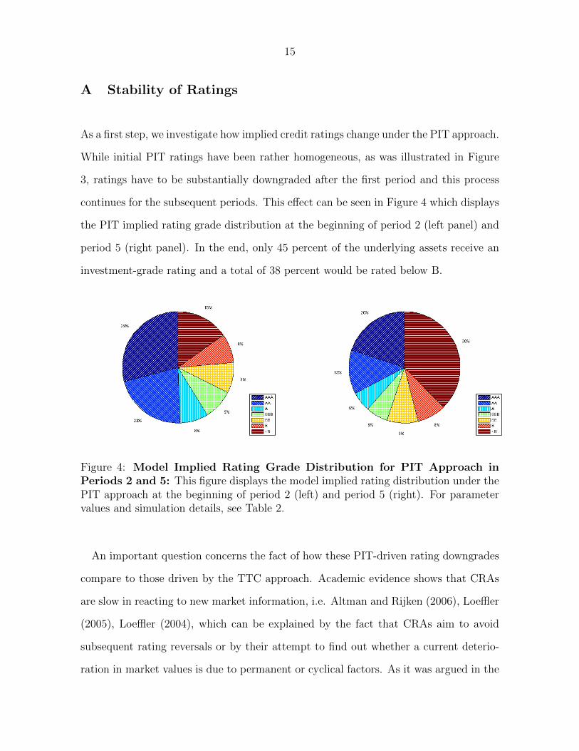
As a first step, we investigate how implied credit ratings change under the PIT approach.

While initial PIT ratings have been rather homogeneous, as was illustrated in Figure

3, ratings have to be substantially downgraded after the first period and this process

continues for the subsequent periods. This effect can be seen in Figure 4 which displays

the PIT implied rating grade distribution at the beginning of period 2 (left panel) and

period 5 (right panel). In the end, only 45 percent of the underlying assets receive an

investment-grade rating and a total of 38 percent would be rated below B.

Figure 4: Model Implied Rating Grade Distribution for PIT Approach inPeriods 2 and 5: This figure displays the model implied rating distribution under thePIT approach at the beginning of period 2 (left) and period 5 (right). For parametervalues and simulation details, see Table 2.

An important question concerns the fact of how these PIT-driven rating downgrades

compare to those driven by the TTC approach. Academic evidence shows that CRAs

are slow in reacting to new market information, i.e. Altman and Rijken (2006), Loeffler

(2005), Loeffler (2004), which can be explained by the fact that CRAs aim to avoid

subsequent rating reversals or by their attempt to find out whether a current deterio-

ration in market values is due to permanent or cyclical factors. As it was argued in the

16

previous section, we will illustrate the effect of a lagged reaction to new information by

using one possible smoothing rule discussed in Cantor and Mann (2006) which proposes

to adjust ratings only (1) if the new rating is at least two notches below the old one

and (2) if the change is persistent, that is if it prevails for more than 1 period.9

Given the smoothing rule, rating downgrades under the TTC approach may take place

in period 3, 4 and 5. It turns out that each period there are on average 57 downgrades

under the TTC methodology whereas under the PIT approach 196 downgrades take

place.10 To further compare the implications of the two rating methodologies with

respect to rating stability, we (1) display rating downgrades under the PIT approach;

(2) the TTC approach under the smoothing rule; and (3) show what would happen

in case CRAs immediately switched from TTC to PIT rating once a stress scenario is

breached.

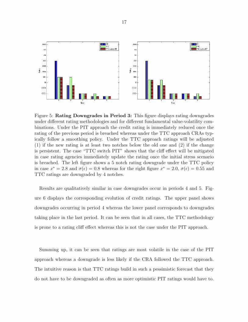
Figure 5 displays two examples of severe rating downgrades which take place in

period 3. The left panel shows that by following a smoothed TTC rating policy, the

credit rating would need to be downgraded by 5 notches under the TTC approach.

Specifically, for the case of an entity with an initial fundamental asset value of x∗ = 2.8

and a corresponding volatility of σ(ε) = 0.8, the TTC rating would drop from BB-

to CCC- whereas the downgrade effect is more smoothed in case the CRA followed a

PIT approach or immediately switched to it once the initial pessimistic forecast was

breached. A similar effect is shown in the right panel where the rating cliff effect under

the TTC methodology amounts to 4 notches.

9Clearly, if the rating of an entity is CCC- then there is no room for a 2 notch downgrade. In thatcase, we adjust the rating to D with a 1 period lag.

10To be precise, in period 3 there are 62 (202) downgrades under the TTC (PIT) approach, in period4 there are 44 (186) downgrades and in period 5 there are 66 (172) respectively. In addition, there are225 downgrades under the PIT approach in period 2.

17

Figure 5: Rating Downgrades in Period 3: This figure displays rating downgradesunder different rating methodologies and for different fundamental value-volatility com-binations. Under the PIT approach the credit rating is immediately reduced once therating of the previous period is breached whereas under the TTC approach CRAs typ-ically follow a smoothing policy. Under the TTC approach ratings will be adjusted(1) if the new rating is at least two notches below the old one and (2) if the changeis persistent. The case “TTC switch PIT” shows that the cliff effect will be mitigatedin case rating agencies immediately update the rating once the initial stress scenariois breached. The left figure shows a 5 notch rating downgrade under the TTC policyin case x∗ = 2.8 and σ(ε) = 0.8 whereas for the right figure x∗ = 2.0, σ(ε) = 0.55 andTTC ratings are downgraded by 4 notches.

Results are qualitatively similar in case downgrades occur in periods 4 and 5. Fig-

ure 6 displays the corresponding evolution of credit ratings. The upper panel shows

downgrades occurring in period 4 whereas the lower panel corresponds to downgrades

taking place in the last period. It can be seen that in all cases, the TTC methodology

is prone to a rating cliff effect whereas this is not the case under the PIT approach.

Summing up, it can be seen that ratings are most volatile in the case of the PIT

approach whereas a downgrade is less likely if the CRA followed the TTC approach.

The intuitive reason is that TTC ratings build in such a pessimistic forecast that they

do not have to be downgraded as often as more optimistic PIT ratings would have to.

18

Figure 6: Rating Downgrades in Periods 4 and 5: This figure displays ratingdowngrades in periods 4 (top) and 5 (bottom) under different rating methodologies andfor different fundamental value-volatility combinations. The upper-left figure shows a5 notch rating downgrade in period 4 under the TTC policy in case x∗ = 3.2 andσ(ε) = 0.75 whereas for the upper-right figure x∗ = 1.6, σ(ε) = 0.45 and TTC ratingsare downgraded by 4 notches in period 4. The lower-left figure shows a 4 notch ratingdowngrade in period 5 under the TTC policy in case x∗ = 2.2 and σ(ε) = 0.45 whereasfor the lower-right figure x∗ = 3.0, σ(ε) = 0.60 and TTC ratings are downgraded by 4notches in period 5. Details regarding different rating methodologies are provided inFigure 5.

19

However, as time passes the actual PIT rating eventually drops below the TTC rating

which is precisely the point when the TTC approach may lead to a rating cliff effect.

Unless this adjustment takes place immediately, the effect can be as large as 5 notches

and may even result in an immediate jump to default, as illustrated in the upper right

panel of Figure 6. It is important to stress that this rating cliff effect does not relate

to the initial stress scenario but to the second stage, i.e. the attempt to filter out

the market data and the subsequent lagged reaction. If a CRA instead immediately

switched to the PIT approach once the initial stress scenario has been breached then

the trade-off between rating stability and accuracy would be maximized.

B Predictive Power of Ratings

While rating stability is an important feature of credit ratings, investors also expect

ratings to accurately reflect the default risk of the underlying asset. We therefore inves-

tigate how well both approaches predict future defaults by computing the Cumulative

Accuracy Profile (CAP) for defaults taking place at the end of each year. CAP curves

are used by the CRAs to measure how accurately their ratings measure the ordinal

ranking of default risk. The CAP profile is derived by comparing the cumulative pro-

portion of defaulters predicted by a specific rating grade to the overall proportion of

assets rated with the specific grade.11

11More specifically, the CAP curve is derived by plotting out the cumulative proportion of entities byrating grade (starting by the lowest grade on the left) against the cumulative proportion of defaultersby rating grade. “Ideal” CAP curves look almost like vertical lines starting at the zero point on thex axis because all the defaulters should be among the lowest rated issuers. In the “random” curve,all defaults occur randomly throughout the rating distribution (admittedly an unrealistically low barfor a CRA), so it lies along the diagonal. The closer the CAP curve to the ideal curve, the better thediscriminatory power of that CRA’s ratings. For more on CAP curves, see Cantor and Mann (2003).

20

Ex ante, it is not fully clear whether the TTC or the PIT methodology delivers

more accurate ratings. On one hand, the TTC approach incorporates more pessimistic

assumptions such that it should be able to better forecast defaults. On the other hand,

PIT ratings are more granular for lower rated assets which by construction leads to an

improved forecasting performance. Figure 7 shows the CAP under the TTC and PIT

methodologies in case defaults occur at the end of the first period. It turns out that

initially the TTC approach is only slightly inferior in forecasting future defaults.

0 0.02 0.04 0.06 0.08 0.1 0.12 0.14 0.16 0.18 0.20

0.1

0.2

0.3

0.4

0.5

0.6

0.7

0.8

0.9

1

Observations Included

De

fau

lts I

nclu

de

d

PIT

TTC

Figure 7: Cumulative Accuracy Profile (CAP) in Period 1: This figure displaysthe CAP under the TTC and PIT rating methodology for defaults occurring at the endof period 1. The CAP curve is derived by plotting out the cumulative proportion ofentities by rating grade against the cumulative proportion of defaulters by rating grade.

To assess the performance of rating methodologies over time, we then compute the

CAP for defaults occurring in subsequent periods. Figure 8 shows CAPs for periods 2, 3,

4 and 5 which are derived by comparing ratings at the beginning of the respective period

to end-of-period defaults. As expected, the PIT approach performs better in period 2

(upper left) given that ratings under the TTC methodology are unaltered with respect

to the previous period. Once TTC ratings are updated, as is the case in period 3 (upper

21

right), both approaches predict future defaults roughly to the same degree. In fact, it

seems that the TTC approach even provides slightly better default forecasts. While

puzzling at first sight, the fact that TTC downgrades reflect significant and persistent

changes in the underlying credit quality, results in a more granular rating distribution

for lower quality entities which improves the performance. For subsequent periods, the

PIT approach again dominates and on average performs better when predicting future

defaults. The intuitive reason is that once the TTC ratings are downgraded, which by

construction occurs for the worst performing assets, subsequent ratings are not updated

immediately which is why ex-post the forecasting performance decreases again. The

lower part of Figure 8 visualizes the corresponding results for periods 4 (left) and 5

(right).

Summing up, it can be seen that the TTC rating methodology suffers from an inferior

forecasting ability relative to the PIT approach. Results suggest that this is not driven

by the initial stress scenario (which makes low quality ratings less granular) but instead

by the reluctance to update ratings immediately once the stress scenario has been

breached. Because new information is not immediately incorporated into ratings, the

forecasting ability deteriorates such that PIT ratings provide more accurate information

regarding the default probability of the underlying asset.

V Summary

The paper employs a simple structural credit risk model to compare two widely used

rating methodologies. Specifically, the analysis compares the PIT and TTC rating

approaches with regards to rating stability and accuracy. Results show that while TTC

22

0 0.02 0.04 0.06 0.08 0.1 0.12 0.14 0.16 0.18 0.20

0.1

0.2

0.3

0.4

0.5

0.6

0.7

0.8

0.9

1

Observations Included

Defa

ults Inclu

ded

PIT

TTC

0 0.02 0.04 0.06 0.08 0.1 0.12 0.14 0.16 0.18 0.20

0.1

0.2

0.3

0.4

0.5

0.6

0.7

0.8

0.9

1

Observations Included

Defa

ults Inclu

ded

PIT

TTC

0 0.02 0.04 0.06 0.08 0.1 0.12 0.14 0.16 0.18 0.20

0.1

0.2

0.3

0.4

0.5

0.6

0.7

0.8

0.9

1

Observations Included

Defa

ults Inclu

ded

PIT

TTC

0 0.02 0.04 0.06 0.08 0.1 0.12 0.14 0.16 0.18 0.20

0.1

0.2

0.3

0.4

0.5

0.6

0.7

0.8

0.9

1

Observations Included

Defa

ults Inclu

ded

PIT

TTC

Figure 8: Cumulative Accuracy Profile (CAP) in Periods 2, 3, 4 and 5: Thisfigure displays the CAP under the TTC and PIT rating methodology for defaults oc-curring at the end of period 2 (upper left), period 3 (upper right), period 4 (lower left)and period 5 (lower right).

implied credit ratings are initially more stable, they are prone to rating cliff effects and

suffer from an inferior ability to predict future defaults.

Specifically, the problem inherent in the TTC approach relates to the fact that, in

a second stage, ratings are typically smoothed and not adjusted immediately. The

analysis has shown that this lagged reaction can potentially lead to rating cliff effects,

i.e. initially stable ratings are prone to a sudden several notches rating downgrade.

Clearly, this abrupt change in the credit rating may lead to a market disruption and

23

dangerous forced selling.

When assessing the predictive power of the two rating approaches, one can observe

a similar picture. While the PIT approach is always superior in forecasting future

defaults, much of the superiority relates to the lagged reaction policy inherent in the

TTC approach.

Summarizing, this study has shown that the TTC approach has positive effects on

rating stability from an ex-ante point of view, that is as long as the underlying stress sce-

nario has not been breached. During this period, TTC ratings promote rating stability

and are only slightly less accurate in predicting future defaults than the PIT approach.

However, once current ratings drop below those implied by the TTC approach, the

TTC approach becomes prone to procyclical rating cliff effects and it suffers from a

clearly inferior ability to predict future defaults. Current discussions on the usefulness

of the TTC approach should therefore focus on the reaction to new information once the

lower asset value, related to the initial stress scenario, is reached. The implementation

of a “through the crisis” approach which has been mentioned by the CRAs themselves,

seems to require a more severe stress test ex-ante, but it currently does not address the

slow adjustment typically taking place once the cushion built in by a TTC approach is

eroded nor the potential cliff effects due to an inefficient smoothing policy.

24

References

Mark Adelson, Gail I. Hessol, Francis Parisi, and Colleen Woodell. Methodology: Credit

stability criteria. Standard and Poor’s: RatingsDirect, 2010.

Edward I. Altman and Herbert A. Rijken. A point-in-time perspective on through-the-

cycle ratings. Financial Analyst Journal, 62:54–70, 2006.

Rodrigo Araya, Yasmine Mahdavi, and Rachid Ouzidane. Moody’s approach to rating

u.s. reit cdos. Moody’s Investor Service, pages 1–14, 2010.

Richard Cantor and Chris Mann. Are corporate bond ratings procyclical? Special

Comment Moody’s Investors Service, 2003.

Richard Cantor and Chris Mann. Analyzing the tradeoff between ratings accuracy and

stability. Special Comment Moody’s Investors Service, 2006.

Mark Carey and Mark Hrycay. Parametrizing credit risk models with rating data.

Journal of Banking and Finance, 25:197–270, 2001.

Eugene Fama and Kenneth French. Permanent and temporary components of stock

prices. Journal of Political Economy, 96:246–273, 1988.

Dale F. Gray, Robert C. Merton, and Bodie Zvi. Contingent claims approach to mea-

suring and managing sovereign credit risk. Journal of Investment Management, 5:

5–28, 2007.

Gunter Loeffler. An anatomy of rating through the cycle. Journal of Banking and

Finance, 28:695–720, 2004.

Gunter Loeffler. Avoiding the rating bounce: why rating agencies are slow to react

25

to new information. Journal of Economic Behavior and Organization, 56:365–381,

2005.

Rebekka Topp and Robert Perl. Through the cycle ratings versus point in time ratings

and implications of the mapping between both rating types. Financial Markets,

Institutions and Instruments, 19:47–61, 2010.

26

V

VI Appendix

A Derivation of Worst Case Scenario

The cyclical component (yt) is assumed to follow a first-order autoregressive process

[AR(1)] with 0 < ρ < 1 and i.i.d. normally-distributed error terms [ut v N(0, σ2u) and

Cov(εt, ut) = 0]:

yt = ρyt−1 + ut (11)

The solution for yt+v can be found through recursive substitution to get:

yt+v = ρvyt + ut+v + ρut+v−1 + ρ2ut+v−2 + ...+ ρv−1ut (12)

Focusing on the terms involving the error parts, it follows that mean and variance are

given by

E[ut+v + ρut+v−1 + ρ2ut+v−2 + ...+ ρv−1ut] = 0

E[(ut+v + ρut+v−1 + ρ2ut+v−2 + ...+ ρv−1ut)2] = σ2

u + ρ2σ2u + ρ4σ2

u + +ρ6σ2u + ...+ ρ2(v−1)σ2

u

= σ2u

(1 + ρ2 + ρ4 + ρ6 + ...ρ2(v−1)

)(13)

27

Thus, the lower bound for the prediction interval, denoted as yt+12 is given by

yt+v = E(yt+v) + Φ−1[p(S)]σu

√(1 + ρ2 + ρ4 + ρ6 + ...ρ2(v−1)) (14)

28

B Rating Mapping

Figure 9: Idealized Default Probability Moody’s Investor Service (Araya et al. (2010)).