Random vicious walks and random matrices Jinho Baik * February 26, 2000 Abstract A lock step walk is a one-dimensional integer lattice walk in discrete time. Suppose that initially there are infinitely many walkers on the non-negative even integer sites. At each moment of time, every walker moves either to its left or to its right with equal probability. The only constraint is that no two walkers can occupy the same site at the same time. Hence we describe the walk as vicious. It is proved that as time tends to infinity, a certain limiting conditional distribution of the displacement of the leftmost walker is identical to the limiting distribution of the (scaled) largest eigenvalue of a random GOE matrix (GOE Tracy- Widom distribution). The proof is based on the bijection between path configurations and semistandard Young tableaux established recently by Guttmann, Owczarek and Viennot. The distribution of semistandard Young tableaux is analyzed using the Hankel determinant expression for the probability obtained from the work of Rains and the author. The asymptotics of the Hankel determinant are then obtained by applying the Deift-Zhou steepest-descent method to the Riemann-Hilbert problem for the related orthogonal polynomials. 1 Introduction In [13], two types of random vicious walks, known as random turn walks and lock step walks, are considered. In these models, walkers are on a one-dimensional integer lattice, and time is discrete. For their applications and earlier results, see for example, [13, 16, 17, 18, 19, 7, 8, 15] and references therein. In this paper we present results on lock step walks, showing a relation to random matrix theory. For similar results of random turn walks, see [15, 5] and discussions after Theorem 1.1 below. Initially, there are infinitely many particles at the sites {0, 2, 4, 6, ···}. We label the walkers by P 1 ,P 2 ,P 3 , ··· from the left to the right. At each (discrete) time t = n, all the particles move either to their right or to their left with equal probability. The only constraint is that no two particles can occupy the same site at the same time. This is why the walkers are called “vicious”. One typical path configuration is shown in Figure 1. This model can also be thought of as a certain totally asymmetric exclusion process in discrete time. Initially there are infinitely many particles at {1, 2, 3, ···}. A particle is called left-movable if its left site is vacant. Particles P j +1 ,P j +2 , ··· ,P k are called successors of a particle P j if they are next to each other in the order of the indices. At each time step, a left-movable particle either stays at its site (hence all it successors * Princeton University and Institute for Advanced Study, New Jersey, [email protected] 1

Welcome message from author
This document is posted to help you gain knowledge. Please leave a comment to let me know what you think about it! Share it to your friends and learn new things together.
Transcript

Random vicious walks and random matrices
Jinho Baik∗
February 26, 2000
Abstract
A lock step walk is a one-dimensional integer lattice walk in discrete time. Suppose that initially there
are infinitely many walkers on the non-negative even integer sites. At each moment of time, every walker
moves either to its left or to its right with equal probability. The only constraint is that no two walkers
can occupy the same site at the same time. Hence we describe the walk as vicious. It is proved that as
time tends to infinity, a certain limiting conditional distribution of the displacement of the leftmost walker is
identical to the limiting distribution of the (scaled) largest eigenvalue of a random GOE matrix (GOE Tracy-
Widom distribution). The proof is based on the bijection between path configurations and semistandard
Young tableaux established recently by Guttmann, Owczarek and Viennot. The distribution of semistandard
Young tableaux is analyzed using the Hankel determinant expression for the probability obtained from the
work of Rains and the author. The asymptotics of the Hankel determinant are then obtained by applying the
Deift-Zhou steepest-descent method to the Riemann-Hilbert problem for the related orthogonal polynomials.
1 Introduction
In [13], two types of random vicious walks, known as random turn walks and lock step walks, are considered.
In these models, walkers are on a one-dimensional integer lattice, and time is discrete. For their applications
and earlier results, see for example, [13, 16, 17, 18, 19, 7, 8, 15] and references therein. In this paper we present
results on lock step walks, showing a relation to random matrix theory. For similar results of random turn
walks, see [15, 5] and discussions after Theorem 1.1 below.
Initially, there are infinitely many particles at the sites {0, 2, 4, 6, · · ·}. We label the walkers by P1, P2, P3, · · ·from the left to the right. At each (discrete) time t = n, all the particles move either to their right or to their
left with equal probability. The only constraint is that no two particles can occupy the same site at the same
time. This is why the walkers are called “vicious”. One typical path configuration is shown in Figure 1.
This model can also be thought of as a certain totally asymmetric exclusion process in discrete time.
Initially there are infinitely many particles at {1, 2, 3, · · ·}. A particle is called left-movable if its left site is
vacant. Particles Pj+1, Pj+2, · · · , Pk are called successors of a particle Pj if they are next to each other in the
order of the indices. At each time step, a left-movable particle either stays at its site (hence all it successors∗Princeton University and Institute for Advanced Study, New Jersey, [email protected]
1

P1 P2 P3 P5 P6P4 P8P7
t
0
2
3
4
5
6
1
Figure 1: vicious lock step walks
stay, too), or moves to its left site together with an arbitrary number of its successors. It is easy to see that
this process is equivalent to the lock step walk described above ; a right move of lock step walk corresponds
to staying at the same site in the exclusion process. Figure 2 represents an exclusion process equivalent to the
lock step walk in Figure 1.
P2P1 P8P7P6P5P3 P4
t
0
2
3
4
5
6
1
Figure 2: exclusion process
In the lock step walk, suppose that a total of k left moves are made by all the particles during N time
steps. In the example of Figure 1, we have N = 6 and k = 14. We denote by P(N, k) the set of all path
configurations during N time steps with a total of k left moves. This is a finite set and each configuration
has equal probability, 1 over the cardinal of P(N, k). Hence our probability space is P(N, k) with uniform
probability given by 1/|P(N, k)|. We denote by Lj(N, k)(π) the number of left moves made by the particle
Pj in a path π ∈ P(N, k). We are interested in the limiting statistics of the random variables Lj(N, k) as
N, k →∞.
2

To state the main result, we need some definitions. Let u(x) be the solution of the differential equation
uxx = 2u3 + xu, u(x) ∼ −Ai(x) as x→ +∞, (1.1)
where Ai is the Airy function. The above equation is called the Painleve II equation. It is known that there
is a unique global solution to (1.1) and the asymptotics as x→ −∞ is established (see, e.g. [2] and references
therein). Define the function, called the GOE Tracy-Widom distribution function, by
F1(x) = exp{− 1
2
∫ ∞x
(s− x)(u(s))2ds+12
∫ ∞x
u(s)ds}. (1.2)
This is indeed a distribution function, and the decay rate is given by
F1(x) = 1 + O(e−cx3/2
), as x→ +∞, (1.3)
F1(x) = O(e−c|x|3), as x→ −∞, (1.4)
for some c > 0 (see, e.g. (2.11)-(2.14) of [4]). In [30], Tracy and Widom proved that F1 is the limiting
distribution of the properly centered and scaled largest eigenvalue of a random matrix taken from a Gaussian
orthogonal ensemble. The subscript 1 in F1 is a general convention : there are also GUE and GSE Tracy-Widom
distribution functions denoted by F2 and F4 [29, 30]. One can find general discussions on random matrices in
[24, 9].
Now the main theorem is
Theorem 1.1. For fixed 0 < t < 1, let
η(t) =2t
1 + t, ρ(t) =
(t(1− t)
)1/31 + t
. (1.5)
Let F1(x) be the GOE Tracy-Widom distribution function. Under the condition that in N time steps a total of
k left moves are made, the (conditional) probability distribution of the number L1(N, k) of left moves made by
the leftmost particle satisfies
limN→∞
P(L1(N, k) − η(t)N
ρ(t)N1/3≤ x
)= F1(x), where k =
t2
1− t2N2 + o(N4/3). (1.6)
Also all the moments of the scaled random variable converge to the corresponding moments of the limiting
random variable.
In other words, as N tends to infinity, the (conditional) fluctuation of the displacement of the leftmost
particle in a lock step walk is identical to the fluctuation of the largest eigenvalue of a random GOE matrix.
Naturally we expect that the kth particle corresponds to the kth eigenvalue of random GOE matrix.
It is of interest to compare the above result with the results for random turn walks. Initially there are
infinitely many walkers Q1, Q2, Q3, · · · at the positions {1, 2, 3, · · ·}. We again call a walker left-movable if its
left site is vacant. At each time, we select one walker at random among left-movable walkers, and move it to
its left site. Hence there is one and only one movement at each time and all the movements are to the left. An
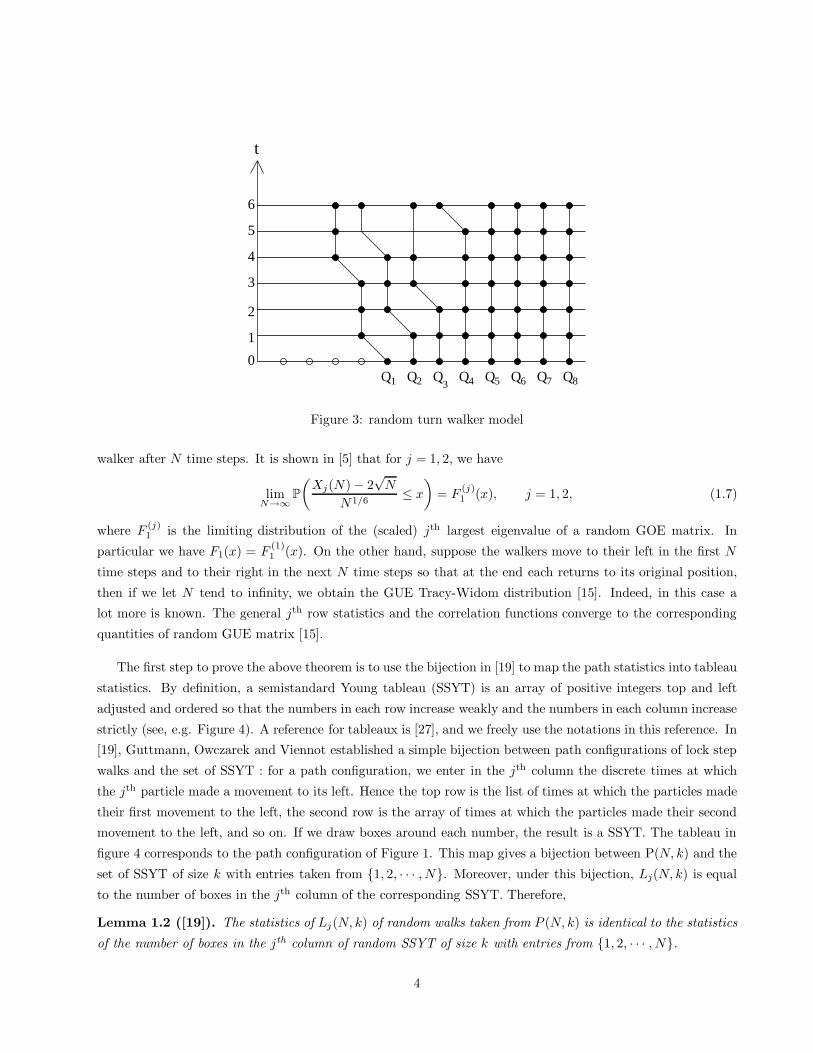
example of random turn walker path configuration is in Figure 3. Let Xj(N) be the displacement of the jth
3
Q5 Q6 Q7 Q8Q1 Q2 Q3
Q4
t
0
2
3
4
5
6
1
Figure 3: random turn walker model
walker after N time steps. It is shown in [5] that for j = 1, 2, we have
limN→∞
P(Xj(N)− 2
√N
N1/6≤ x
)= F
(j)1 (x), j = 1, 2, (1.7)
where F(j)1 is the limiting distribution of the (scaled) jth largest eigenvalue of a random GOE matrix. In
particular we have F1(x) = F(1)1 (x). On the other hand, suppose the walkers move to their left in the first N
time steps and to their right in the next N time steps so that at the end each returns to its original position,
then if we let N tend to infinity, we obtain the GUE Tracy-Widom distribution [15]. Indeed, in this case a
lot more is known. The general jth row statistics and the correlation functions converge to the corresponding
quantities of random GUE matrix [15].
The first step to prove the above theorem is to use the bijection in [19] to map the path statistics into tableau
statistics. By definition, a semistandard Young tableau (SSYT) is an array of positive integers top and left
adjusted and ordered so that the numbers in each row increase weakly and the numbers in each column increase
strictly (see, e.g. Figure 4). A reference for tableaux is [27], and we freely use the notations in this reference. In
[19], Guttmann, Owczarek and Viennot established a simple bijection between path configurations of lock step
walks and the set of SSYT : for a path configuration, we enter in the jth column the discrete times at which
the jth particle made a movement to its left. Hence the top row is the list of times at which the particles made
their first movement to the left, the second row is the array of times at which the particles made their second
movement to the left, and so on. If we draw boxes around each number, the result is a SSYT. The tableau in
figure 4 corresponds to the path configuration of Figure 1. This map gives a bijection between P(N, k) and the
set of SSYT of size k with entries taken from {1, 2, · · · , N}. Moreover, under this bijection, Lj(N, k) is equal
to the number of boxes in the jth column of the corresponding SSYT. Therefore,
Lemma 1.2 ([19]). The statistics of Lj(N, k) of random walks taken from P (N, k) is identical to the statistics
of the number of boxes in the jth column of random SSYT of size k with entries from {1, 2, · · · , N}.
4

56
4
32 2 33 4
1 1 16
Figure 4: semistandard Young tableau
After the work of Guttmann, Owczarek and Viennot, in [15] Forrester observed that a similar bijection can
be established between the set of path configurations of random turn walks and the set of standard Young
tableaux (SYT). The above result (1.7) is obtained based on this bijection and the recent work in [4] on the
statistics of the first row of random SYT. Also as mentioned above, supposing that the walkers move to their left
in the first N time steps and then move to their right in the next N time steps so that at the end each returns
to its original position, the limiting fluctuation is not GOE type, but GUE type. This difference comes from
the fact that in this case the path configuration is in bijection with the pairs of SYT. The theory concerning
statistics of pairs of SYT is more well developed than that of single SYT [2, 1, 25, 6, 20], and hence we have
the stronger results mentioned earlier.
This paper is organized as follows. In Section 2 using the result of [3], we express the generating function
for the probability of the first column of random tableaux in terms of a Hankel determinant. From a general
theory of orthogonal polynomials, this Hankel determinant is related to certain orthogonal polynomials on the
unit circle. The asymptotics of the orthogonal polynomials are obtained by using a Riemann-Hilbert approach
and applying the Deift-Zhou steepest descent method. These results are summarized separately in Section 3.
Finally, we can obtain the limiting statistics of the first column from the knowledge of the Hankel determinant
asymptotics. This work occupies the second half of Section 2 and the proof of Theorem 1.1 is given at the end
of Section 2.
Acknowledgement.
The author would like to thank Percy Deift for his interest and encouragement.
2 Proof
Let dλ(N) be the number of semistandard Young tableaux of shape λ with entries from {1.2. · · · , N}, and let
`(λ) be the number of rows of λ (parts of λ, or the length of the first column). From the bijection of path
configurations and tableaux, Lemma 1.2, the number of path π ∈ P(N, k) satisfying L1(N, k)(π) ≤ l is equal to∑λ`k`(λ)≤l
dλ(N). (2.1)
5
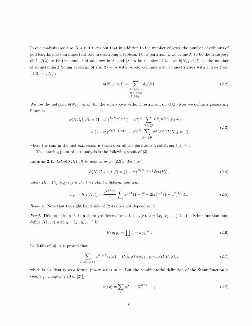
In our analysis (see also [3, 4]), it turns out that in addition to the number of rows, the number of columns of
odd lengths plays an important role in describing a tableau. For a partition λ, we define λ′ to be the transpose
of λ, f(λ) to be the number of odd row in λ, and |λ| to be the size of λ. Let b(N, j,m, l) be the number
of semistandard Young tableaux of size 2j + m with m odd columns with at most l rows with entries from
{1, 2, · · · , N} :
b(N, j,m, l) =∑
λ`2j+mf(λ′)=m`(λ)≤l
dλ(N). (2.2)
We use the notation b(N, j,m,∞) for the sum above without restriction on `(λ). Now we define a generating
function
φ(N, l, t, β) := (1− t2)N(N−1)/2(1− βt)N∑`(λ)≤l
t|λ|βf(λ′)dλ(N)
= (1− t2)N(N−1)/2(1− βt)N∑j,m≥0
t2j(βt)mb(N, j,m, l),(2.3)
where the sum in the first expression is taken over all the partitions λ satisfying `(λ) ≤ l.The starting point of our analysis is the following result of [3].
Lemma 2.1. Let φ(N, l, t, β) be defined as in (2.3). We have
φ(N, 2l+ 1, t, β) = (1− t2)N(N−1)/2 det(Hl), (2.4)
where Hl = (hjk)0≤j,k<l is the l × l Hankel determinant with
hjk = hjk(N, t) =2j+k+1
π
∫ 1
−1
xj+k(1 + t2 − 2tx)−N(1− x2)1/2dx. (2.5)
Remark. Note that the right hand side of (2.4) does not depend on β.
Proof. This proof is in [3] in a slightly different form. Let sλ(x), x = (x1, x2, · · · ), be the Schur function, and
define H(u; y) with y = (y1, y2, · · · ) by
H(u; y) =∏j
(1− uyj)−1. (2.6)
In (5.65) of [3], it is proved that∑`(λ)≤2l+1
βf(λ′)sλ(x) = H(β; x)EU∈Sp(2l) det(H(U ; x)), (2.7)
which is an identity as a formal power series in x. But the combinatorial definition of the Schur function is
(see, e.g. Chapter 7.10 of [27])
sλ(x) =∑T
xα1(T )1 x
α2(T )2 · · · , (2.8)
6
where the sum is over all semistandard Young tableaux T of shape λ, and αj(T ) is the number of parts of T
equal to j (type of T ). Since∑j αj(T ) = |λ|, if we take the special case x = (t, t, · · · , t, 0, 0, · · ·) where the first
N elements are t and the rest are 0, then sλ(x) becomes
t|λ|dλ(N). (2.9)
Hence for this special choice of x (2.7) is now∑`(λ)≤2l+1
βf(λ′)t|λ|dλ(N) = (1− βt)−N EU∈Sp(2l) det((1 − tU)−N ). (2.10)
Now using Weyl’s integration formula for Sp(2l) (see, e.g. [26]), the expectation in (2.10) becomes
EU∈Sp(2l) det((1− tU)−N )
=2l
2
l!(2π)l
∫[0,2π]l
∏1≤j<k≤l
(cos θj − cos θk)2l∏
j=1
sin2 θjdθj
(1 + t2 − 2t cos θj)N(2.11)
Standard Vandermonde determinant manipulations yield that this is equal to
2l2
(2π)ldet(∫ 2π
0
cosj+k θ sin2 θ(1 + t2 − 2t cos θ)−N dθ)
0≤j,k<l. (2.12)
After change of variables x = cos θ, this is again equal to
2l2
πldet(∫ 1
−1
Uj(x)Uk(x)(1 + t2 − 2tx)−N (1− x2)1/2dx
)0≤j,k<l
(2.13)
where Uj(x) = sin((j+1)θ)sin θ
, x = cos θ, is the Chebyshev polynomial of the second kind. Note that Uj(x) =
2jxj + · · · . Hence elementary row and column operations imply Lemma 2.1.
Using this expression, we first obtain the asymptotic result for the generating function. The limit is insen-
sitive to β since so is φ. Assuming the results of Proposition 3.2, we have
Proposition 2.2. Let 0 < t < 1 and β > 0 be fixed satisfying 0 < βt < 1. For each l and N , define x ∈ R by
x =l − η(t)Nρ(t)N1/3
, (2.14)
where η(t) and ρ(t) are defined in (1.5) Then there exits a positive constant M0 such that for M > M0, there
are constants C, c > 0, independent of M , and C(M) which may depend on M so that
|φ(N, l, t, β)− F1(x)| ≤ C(M)l1/3
+ Ce−cM3/2, −M < x < M. (2.15)
Also we have
0 ≤ 1− φ(N, l, t, β) ≤ Ce−cx3/2, x ≥M0, (2.16)
0 ≤ φ(N, l, t, β) ≤ Ce−c|x|3, x ≤ −M0. (2.17)
7

Proof. It is enough to consider the limit for φ(N, 2l + 1, t, β) since from the definition (2.3), φ is monotone
increasing in l. First we relate the determinant in (2.4) with certain quantities of orthogonal polynomials on
the circle.
Let pj(x) = xj + · · · be the jth monic orthogonal polynomial with respect to the weight w(x)dx = (1 + t2−2tx)−N(1− x2)1/2dx on the interval (−1, 1), and let Cj be the norm of pj :∫ 1
−1
pj(x)pk(x)w(x)dx = Cjδjk. (2.18)
It is a well known result of orthogonal polynomial theory (see, e.g. [28]) that Cj = det(Hj+1)/ det(Hj), where
Hl = (hjk)0≤j,k<l with
hjk =∫ 1
−1
xj+k(1 + t2 − 2tx)−N(1 − x2)1/2dx, (2.19)
which is equal to π2j+k+1 hjk (recall (2.5)). Hence det(Hj) = πj
2j2 det(Hj). Since the Szego strong limit theorem
for Hankel determinants (see, e.g. [21]) implies that liml→∞ det(Hl) = (1− t2)−N(N−1)/2 for fixed N , we have
φ(N, 2l+ 1, t, β) = limk→∞
k∏j=l
det(Hj)det(Hj+1)
=∞∏j=l
π
22j+1C−1j . (2.20)
Now we use the relation between orthogonal polynomials on the unit circle and those on the interval (−1, 1).
Let πj(z) = zj + · · · be the jth monic orthogonal polynomials on the unit circle {|z| = 1} with respect to the
weight
ϕ(z)dz
2πi= (1− tz)−N (1− tz−1)−N
dz
2πiz, (2.21)
and let Nj be the norm of πj(z) : ∫|z|=1
πj(z)πk(z)ϕ(z)dz
2πiz= Njδjk. (2.22)
There is a simple relation between orthogonal polynomials pj on the unit circle and orthogonal polynomials πjon the interval (see the forth equation of (11.5.2) in [28]) : with x = 1
2 (z + z−1),
C−1/2j pj(x) =
√2π
(1 + π2j+2(0)
)−1/2N−1/22j+1
z−jπ2j+1(z)− zjπ2j+1(z−1)z − z−1
. (2.23)
Especially comparing the coefficient of the leading term xj, we have
Cj =π
22j+1
(1 + π2j+2(0)
)N2j+1. (2.24)
But we also have (1− πn+1(0)2)Nn = Nn+1 (see (11.3.6) in [28]). Hence (2.24) is equal to
Cj =π
22j+1
(1− π2j+2(0)
)−1N2j+2. (2.25)
Therefore (2.20) becomes
φ(N, 2l+ 1, t, β) =∞∏j=l
(1− π2j+2(0)
)N−1
2j+2. (2.26)
8

Now using Proposition 3.2, computations similar to Lemma 7.1 of [2] (also Corollary 7.2 and Corollary 7.6 of
[4]) yield the result.
Interpreting the notation b(N, j,m,∞) as the sum without constraints on `(λ) in (2.2), the total number of
path configurations in P(N, k) is equal to
|P(N, k)| =∑
2j+m=k
b(N, j,m,∞), (2.27)
and the probability that L1(N, k) ≤ l is equal to
1|P(N, k)|
∑2j+m=k
b(N, j,m, l) =1
|P(N, k)|∑
2j+m=k
p(N, j,m, l)b(N, j,m,∞), (2.28)
where
p(N, j,m, l) =b(N, j,m, l)b(N, j,m,∞)
. (2.29)
For fixed N , as l →∞, the Szego strong limit theorem for Hankel determinants (see, e.g. [21]) implies that
(2.4) becomes 1. Thus we have the identity∑j,m≥0
t2j(βt)mb(N, j,m,∞) = (1− t2)−N(N−1)/2(1− βt)−N . (2.30)
By comparing the coefficients of t, β, this implies
b(N, j,m,∞) =(N(N−1)
2 + j − 1j
)(N +m− 1
m
). (2.31)
See the remark after Lemma 2.6 below for more direct derivation. Thus from (2.27), the total number of paths
in P(N, k) is equal to
|P(N, k)| =∑
2j+m=k
(N(N−1)2 + j − 1
j
)(N +m− 1
m
). (2.32)
Now it is straightforward to obtain the following result on the number of all paths.
Lemma 2.3. Let 0 < t < 1 and let
k =[ t2
1− t2N2 + o(N4/3)
]. (2.33)
As N →∞, we have
|P(N, k)| =exp{−N2t2
1−t2 log t− µN log t− 14
(µ(1−t2)t − 1
)2}√πtN(1− t)N (1− t2)N(N−1)/2−1
(1 + o(1)
)(2.34)
where the term o(1) vanishes as N →∞, and µ is defined by
µ :=1N
(k − t2
1− t2N2
)(2.35)
9

which is of order o(N1/3) from (2.33). Moreover, the main contribution to the sum comes from |m− t1−tN | ≤
N1/2+ε/2 for some 0 < ε < 13 ; precisely, there is a constant c > 0 such that for any 0 < ε < 1
3 , we have
|P(N, k)| =[ ∑|m− t
1−tN|≤N1/2+ε/2
k−m is even
b(N,k −m
2, m,∞)
](1 + O(e−cN
ε
)). (2.36)
Proof. From (2.32), we have
|P(N, k)| =[k2 ]∑m=0
a(m), (2.37)
where
a(m) =(N(N−1)
2 + k−m2 − 1
k−m2
)(N +m− 1
m
). (2.38)
The ratio of a(m) is
a(m+ 2)a(m)
=(N +m+ 1)(N +m)(k −m)
(m+ 2)(m+ 1)(N(N − 1) + k −m− 2). (2.39)
One can directly check that under the condition (2.33), the above ratio is decreasing in m, and becomes closest
to 1 at
mc =[ t
1− tN + o(N1/3)]. (2.40)
Hence a(m) is unimodal: it is increasing for m < mc and is decreasing for m > mc. Now consider the
neighborhood N of mc of size N1/2+ε/2 for some fixed 0 < ε < 13. For m in N , set
m =t
1− tN + x, |x| ≤ N1/2+ε/2. (2.41)
For any M,x > 0, Stirling’s formula yields
(M + x)! =√
2πMMM+xe−M+ x22M
(1 +O
( xM
)+ O
( x3
M2
)). (2.42)
Using (2.33), (2.41) and (2.42), we have for m in N,
(N +m− 1
m
)=
exp{−( tN
1−t + x) log t− (1−t)2x2
2tN
}√
2πtN(1− t)N−1
(1 +O(N−
12 + 3
2 ε))
(2.43)
and (N(N−1)2 + k−m
2 − 1k−m
2
)
=exp{−( t2
1−t2N2 + (µ− t
1−t)N − x) log t− 14( (1−t2)µ
t − 1)2}
√πtN(1− t2)N(N−1)/2−1
(1 + o(1)
).
(2.44)
10

Thus we have for m satisfying (2.41)
a(m) =exp{−N2t2
1−t2 log t−Nµ log t− 14
(µ(1−t2)t − 1
)2 − (1−t)2x2
2tN
}√
2πt3/2N3/2(1− t)N(1− t2)N(N−1)/2−1
(1 + o(1)
). (2.45)
Let
|P(N, k)| =∑∗a(m) +
∑∗∗a(m), (2.46)
where ∗ denotes the set N of m satisfying (2.41) and ∗∗ denotes the rest of the range of m. From (2.45), the
first sum over ∗ is equal to the right hand side of (2.34). Also from the unimodality, a(m) in ∗∗ is less than or
equal to the largest of a(m+) and a(m−) where m± = [ t1−tN ±N1/2+ε]. The number of summand in ∗∗ is of
order N2. Hence using (2.45) again for m±, if we take c = (1−t)2
4t, for large N , we obtain∑
∗∗a(m) =
(∑∗a(m)
)e−cN
ε
, (2.47)
which establishes the proof.
Now we rewrite (2.3) as
φ(N, l, t, β)
= (1− t2)N(N−1)/2(1− βt)N∑j,m≥0
t2j(βt)mb(N, j,m,∞)p(N, j,m, l). (2.48)
The asymptotics of φ(N, l, t, β) and p(N, j,m, l) are related as follows.
Lemma 2.4. For any d > 0, there are constants C0, c0 > 0 such that for all l ≥ 0,
p(N, µ+(N), ν+(N), l)− C0
Nd≤ φ(N, l, t, β) ≤ p(N, µ−(N), ν−(N), l) +
C0
Nd(2.49)
where
µ±(N) =[
t2
2(1− t2)N2 ± c0N
√logN
], (2.50)
ν±(N) =[
βt
1− βtN ± c0√N logN
]. (2.51)
The proof follows by using the following Lemma twice for j and m indices together with the Lemma 2.6.
(Recall the (2.31)).
Lemma 2.5. For a sequence {qj}j≥0, we define the following generating function
G(N) = (1− a)N∞∑j=0
aj(N + j − 1
j
)qj, 0 < a < 1, N = 1, 2, · · · . (2.52)
For each d > 0, there are constants C1, c1 ≥ 0 such that for any sequence {qj}j≥0 satisfying (i) qj ≥ qj+1 and
(ii) 0 ≤ qj ≤ 1,
qN∗∗ −C1
Nd≤ G(N) ≤ qN∗ +
C1
Nd, N ≥ 1, (2.53)
11

where
N∗ =a
1− aN − c1√N logN, (2.54)
N∗∗ =a
1− aN + c1√N logN. (2.55)
Proof. This proof is parallel to that of the de-Poissonization lemma in [22]. We have
G(N) =∞∑j=0
fjqj, fj = (1− a)Naj(N + j − 1
j
). (2.56)
Stirling’s formula yields for n,m ≥ 1,(m+ n− 1
m
)≤ C exp
{m[(1 +
n
mlog(1 +
n
m)− n
mlog
m
n
]}, (2.57)
with some constant C. Thus we have
fj ≤ C exp{Nh(j/N)}, (2.58)
where
h(x) = (1 + x) log(1 + x)− x logx+ x loga+ log(1− a). (2.59)
One can directly check the following estimates of h :
h(x) ≤ −(1− a)2
2a(x− a
1− a)2, 0 ≤ x ≤ 2a
1− a, (2.60)
h(x) ≤ −[log 2− 1 + a
2alog(1 + a)
]x, x ≥ 2a
1− a. (2.61)
We take a constant c1 > 0 satisfying (1−a)2
2ac21 − 1 ≥ d. From (2.60) and the condition (ii), we have∑
j≤N∗fjqj ≤
a
1− aCNe− (1−a)2
2a c2 logN ≤ C
Nd, (2.62)
with a new constant C. Similarly, ∑N∗∗≤j≤ 2a
1−aN
fjqj ≤C
Nd. (2.63)
Also using (2.61), we have ∑j≥ 2a
1−aN
fjqj ≤ C ′e−c′N (2.64)
for some constants c′, C ′. Thus we have∣∣∣∣G(N)−∑
N∗≤j≤N∗∗fjqj
∣∣∣∣ ≤ C
Nd, (2.65)
12

with a possibly different constant C. Now from the monotonicity condition (i), we have∑N∗≤j≤N∗∗
fjqj ≤( ∑N∗≤j≤N∗∗
fj
)qN∗ ≤ qN∗ , (2.66)
and ∑N∗≤j≤N∗∗
fjqj ≥( ∑N∗≤j≤N∗∗
fj
)qN∗∗ ≥
(1− C
Nd
)qN∗∗ ≥ qN∗∗ −
C
Nd, (2.67)
using the equality (2.65) for the second equality. Thus we obtained the desired result.
To use the above Lemma to φ, we need monotonicity in l. It is more convenient now to view semistandard
Young tableaux (SSYT) as generalized permutations. A two-rowed array
π =
(i1 · · · ik
j1 · · · jk
)(2.68)
is called a generalized permutation if either ir < ir+1 or ir = ir+1, jr ≤ jr+1. Suppose the elements in the
upper row of π come from {1, 2, · · · ,M} and the elements in the bottom row come from {1, 2, · · · , N}. One
can represent a generalized permutation as a M ×N matrix (aik) where aik is the number of times when(ik
)occurs in π. For example, the generalized permutation(
1 1 1 2 2 2 2 3 3
1 3 3 2 2 2 4 3 4
)(2.69)
corresponds to 1 0 2 0
0 3 0 1
0 0 1 1
. (2.70)
In the proof of the Lemma below, we regard a generalized permutation as a M ×N square board with stacks
of aik balls in each position (i, k). We denote by L(π) the length of the longest strictly decreasing subsequence
of π. In the example (2.69), L(π) = 2.
Let Mj,m be the set of N ×N matrices π = (aik) which is symmetric aik = aki, and satisfies∑Ni=1 aii = m
and∑
1≤i<k≤N aik = j. This is a subset of the set of generalized permutations. The celebrated Robinson-
Schensted-Knuth correspondence [23] establishes a bijection between Mj,m and the set of SSYT of size 2j +m
with m odd columns with entries from {1, 2, · · · , N}. Moreover, under this bijection, L(π) for π ∈Mj,m (viewed
as a generalized permutation) is equal to the number of rows of the corresponding SSYT.
With this preliminary, we can prove the following.
Lemma 2.6 (monotonicity). For any j,m ≥ 0, we have
p(N, j + 1, m, l) ≤ p(N, j,m, l), p(N, j,m+ 1, l) ≤ p(N, j,m, l). (2.71)
13

Proof. We first consider the second inequality. From (2.29), we need to show that
(m+ 1)b(N, j,m+ 1, l) ≤ (N +m)b(N, j,m, l). (2.72)
By the definition (2.2) and the Robinson-Schensted-Knuth correspondence, b(N, j,m, l) is equal to the number
of π ∈Mj,m satisfying L(π) ≤ l.Consider all the possibilities of the strict upper triangular part of an element π ∈ Mj,m. It is equal to
putting j identical balls into N(N − 1)/2 boxes ; K =(N(N−1)/2+j−1
j
)distinct ways. Hence we have a disjoint
union Mj,m = ∪Ki=1Si,m where each Si,m consists of π ∈ Mj,m with same upper triangular part, and elements
in Si,m and Si′,m have different upper triangular parts when i 6= i′. Similarly, Mj,m+1 = ∪Ki=1S′i,m+1 where
σ ∈ S′i,m+1 has the upper triangular part same as that of π ∈ Si,m.
Now for each π = (ars) ∈ Si,m, we generate N +m elements in S′i,m+1 as follows. For 1 ≤ r ≤ N , assign
arr+1 identical π′ = (a′kl) such that a′rr = arr+1 and a′kl = akl for (k, l) 6= (r, r). (One can think this as adding
a new ball in the stack of arr balls ; there are arr +1 ways to put a new ball.) Since∑
1≤r≤N(arr +1) = m+N ,
there result (m+N)|Si,m| (many identical) elements of Si,m+1. Note that under this assignment,
L(π′) ≥ L(π). (2.73)
Now fix σ = (bkl) ∈ Si,m+1. Since there are m+ 1 diagonal entries, there are exactly m + 1 (many identical)
elements of Si,m from which σ is generated under the above assignment. (Considering each entry as a ball, each
m+1 balls on the diagonal can be a newly added one.) Thus we have the identity (m+N)|Si,m| = (m+1)|Si,m+1|.Furthermore, from the remark regarding (2.73), we have (m + 1)|Ri,m+1,l| ≤ (m +N)|Ri,m,l|, where Ri,m,l is
the subset of π ∈ Si,m satisfying L(π) ≤ l. Therefore the second inequality in the Lemma is obtained.
The first inequality follows from a similar argument.
Remark. As mentioned before, using the generalized permutation interpretation of SSYT, we can see (2.31)
directly. From non-negative integer matrix representation of generalized permutations, b(N, j,m,∞) is the
number of N×N matrices (ars) with non-negative integer entries such that∑Nr=1 arr = m and
∑1≤r<s≤N ars =
j. It is equivalent to placing m identical balls of color 1 into N boxes and j identical balls of color 2 into
N(N − 1)/2 boxes. Therefore we obtain (2.31).
Now we give the proof of the theorem.
proof of Theorem 1.1. In (2.28), we have
P(L1(N, k) ≤ l) =1
|P (N, k)|∑
2j+m=k
p(N, j,m, l)b(N, j,m,∞). (2.74)
where P (N, k), p(N, j,m, l) and b(N, j,m,∞) are given in (2.32), (2.31) and (2.29), and b(N, j,m, l) is given in
(2.2). We split the above sum into two pieces. One part is the sum over (1) |m− t1−tN | ≤ N1/2+ε/2 and (2)
the rest, where 0 < ε < 13 is fixed. Then since 0 ≤ p(N, j,m, l) ≤ 1, we have from (2.36)
1|P (N, k)|
∑(2)
p(N, j,m, l)b(N, j,m,∞) = O(e−cNε
) (2.75)
14
for some c > 0.
We use Lemma 2.4 to estimate p(N, j,m, l) for (j,m) in (1). Set
t2 =k −m− 2c0N
√logN
N2 + k −m− 2c0N√
logN, (2.76)
β =m− c0
√N logN
N +m− c0√N logN
t−1, (2.77)
where k satisfies the condition in (1.6), and we take t > 0. For (j,m) in (1), they satisfy
t = t + o(N−2/3), β = 1 + O(N−1/2+ε/2). (2.78)
The first inequality of (2.49) yields p(N, j,m, l) ≤ φ(N, l, t, β) + C0N−d. Set x by (2.14) where t is replaced
by t and l is given by l = [η(t)N + xρ(t)N1/3]. Let M > M0 satisfy −M < 2x < M where M0 is given in
Proposition 2.2. From (2.78), we have
x = x+ o(1), (2.79)
Proposition 2.2 implies that with l = [η(t)N + xρ(t)N1/3],
|φ(N, l, t, β)− F1(x)| ≤ C(M)l1/3
+Ce−cM3/2, (2.80)
for large N . Since F ′1(x) = −12(u(x) + v(x))F1(x) is bounded for x ∈ R, we have from (2.79) that F1(x) =
F1(x) + o(1). Thus we have for large N ,
p(N, j,m, l) ≤ F1(x) + o(1), (2.81)
where o(1) term is independent of (j,m) in (1) and vanishes as N → ∞. Thus using Lemma 2.3, we have for
large N ,
P(L1(N, k) ≤ l) ≤ 1|P (N, k)|
∑(1)
(F1(x) + o(1))b(N, j,m,∞) + O(e−cN2ε
)
= F1(x) + o(1), l = [η(t)N + xρ(t)N1/3]
(2.82)
Similarly, we obtain the lower bound using the second inequality of (2.49). Thus we proved (1.6).
The convergence of moments is also similar using (2.16) and (2.17) (cf. Section 8 of [4]).
3 Asymptotics of orthogonal polynomials
This section is devoted to asymptotics of orthogonal polynomials used in the proof of Proposition 2.2. The key
ingredient is the equilibrium measure (see [11, 12, 2]).
Let Σ be the unit circle oriented counterclockwise. The equilibrium measure dµV (z) = ψ(θ) dθ2π for V (z) and
its support J are uniquely determined by the following Euler-Lagrange variational conditions :
there exits a real constant l such that,
2∫
Σ
log |z− s|dµV (s) − V (z) + l = 0 for z ∈ J ,
2∫
Σ
log |z− s|dµV (s) − V (z) + l ≤ 0 for z ∈ Σ− J .
(3.1)
15

Lemma 3.1. Let γ ≥ 0 and 0 < t < 1, and let
V (z) = γ log(1− tz)(1− tz−1). (3.2)
Then their equilibrium measure ψ(θ)dθ/2π is given as follows.
• When 0 ≤ γ ≤ 1+t2t , we have J = Σ, l = 0, and
ψ(θ) = 1− γ +γ(1 − t2)
1 + t2 − 2t cos θ(3.3)
= 1 + γt
(z
1− tz +z−1
1− tz−1
), z = eiθ. (3.4)
• When γ > 1+t2t , we have J = {eiθ : |θ| ≤ θc}, where sin2 θc
2 = (1−t)2(2γ−1)4t(γ−1)2 , 0 < θc < π, or quivalently,
|ξ − t| = γ(1 − t)γ − 1
, ξ = eiθc , (3.5)
and
l = 2γ log(2γ − 1)(1− t)
2(γ − 1)− log
(2γ − 1)(1− t)2
4t(γ − 1)2. (3.6)
Also
ψ(θ) =4(γ − 1) cos θ2
(1−t)2
t+ 4 sin2 θ
2
√sin2 θc
2− sin2 θ
2(3.7)
=(γ − 1)(1 + z)
(z − t)(z − t−1)
√(z − ξ)(z − ξ−1)+, z = eiθ, (3.8)
where√
(z − ξ)(z − ξ−1)+ denotes the limit of z from inside the unit circle. And in this case, the inequality
of the second variational condition in (3.1) is strict for z ∈ Σ \ J .
Proof. The proof given here is similar to the proof of Lemma 4.3 in [2], whose main ingredient is the following
results of Lemma 4.2 in [2] (see [10] for results on the line). Let dµ(s) = u(θ)dθ be an absolutely continuous
probability measure on the unit circle Σ and u(θ) = u(−θ). Define
g(z) =∫
Σ
log(z − s)dµ(s), (3.9)
where for fixed s = eiθ0 ∈ Σ, log(z − s) is defined to be analytic in C \((−∞,−1] ∪ {eiθ : −π ≤ θ ≤ θ0}
), and
log(z − s) ∼ log z for z → +∞ with z ∈ R. Then for z = eiφ ∈ Σ, we have
g+(z) + g−(z) = 2∫
Σ
log |z − s|dµ(s) + i(φ+ π), (3.10)
g+(z) − g−(z) = 2πi∫ π
φ
u(θ)dθ. (3.11)
Also evenness of u yields g(0) = πi.
16
• When 0 ≤ γ ≤ 1+t2t
: By residue calculation, it is easy to check∫ π−π ψ(θ) dθ
2π= 1. Define g(z) =
∫ π−π log(z−
eiθ)ψ(θ) dθ2π as in (3.9). Then by direct residue calculation, we obtain
g′(z) =
−γt1−tz , |z| < 1,γtz−2
1−tz−1 + 1z , |z| > 1.
(3.12)
Since g(0) = πi and g(z) ∼ log(z) as z →∞, we have
g(z) =
γ log(1 − tz) + πi, |z| < 1,
γ log(1 − tz−1) + log z, |z| > 1.(3.13)
Thus, from (3.10), the variational condition (3.1) is satisfied with J = Σ and l = 0.
• When γ > 1+t2t : Set β(z) =
√(z − ξ)(z − ξ−1) which is analytic in C \ J and β(z) ∼ z as z → +∞ with
z ∈ R. Then we have
β(0) = −1, β(t) = −|ξ − t|, β(t−1) =1t|ξ − t|. (3.14)
First, direct residue calculation using (3.14) shows that∫ θc−θc ψ(θ) dθ
2π= 1, hence ψ(θ)dθ/(2π) is a prob-
ability measure. Now we define g(z) =∫ θc−θc log(z − eiθ)ψ(θ) dθ2π as before. Using (3.14) again, residue
calculations yield
g′(z) =12
(1z
+γtz−2
1− tz−1− γt
1− tz
)− (γ − 1)(z + 1)
2z(z − t)(z − t−1)β(z). (3.15)
Thus we have for |z| > 1, z /∈ (−∞,−1) ∪ [t−1,∞),
g(z) =γ
2log(1− tz)(1 − tz−1) +
12
log z
−∫ z
1+0
(γ − 1)(s+ 1)2s(s− t)(s− t−1)
β(s)ds + g−(1) − γ log(1− t),(3.16)
and for |z| < 1, z /∈ (−1, t],
g(z) =γ
2log(1− tz)(1− tz−1) +
12
log z
−∫ z
1−0
(γ − 1)(s+ 1)2s(s− t)(s− t−1)
β(s)ds + g+(1)− γ log(1− t).(3.17)
Now we compute g+(1) + g−(1). From (3.10) with z = 1 and the evenness of ψ, we have
g+(1) + g−(1) − πi
=8(γ − 1)
π
∫ θc
0
log(
2 sinθ
2
)cos θ2
(1−t)2
t + 4 sin2 θ2
√sin2 θc
2− sin2 θ
2dθ.
(3.18)
Substituting x = (sin θc2 )−1 sin θ
2 , the above becomes
4(γ − 1)π
∫ 1
0
log(
2 sinθc2x
)√1− x2
x2 + p2dx, (3.19)
17
with
p :=1− t
2√t sin θc
2
=γ − 1√2γ − 1
. (3.20)
Using 2(γ−1)π
∫ 1
0
√1−x2
x2+p2 dx = 1 which is a consequence of the fact that ψ(θ)dθ/(2π) is a probability measure,
we have
g+(1) + g−(1)− πi = 2 log(
2 sinθc2
)+
4(γ − 1)π
∫ 1
0
log(x)√
1− x2
x2 + p2dx. (3.21)
Now we use∫ 1
0logx dx√
1−x2 =∫ π/2
0log(sin θ)dθ = −π
2log 2 to rewrite the last term in the above as
2(γ − 1) log 2 +4(γ − 1)(1 + p2)
π
∫ 1
0
log x(x2 + p2)
√1− x2
dx. (3.22)
But by residue calculation, we have∫ 1
0
logx(x2 + p2)
√1− x2
dx = −π2
∫ ∞1
dx
(x2 + p2)√x2 − 1
+π logp
2p√
1 + p2. (3.23)
And also one can directly verify that∫dx
(x2 + p2)√x2 − 1
=1
2p√
1 + p2log∣∣∣∣p√x2 − 1 +
√1 + p2x
p√x2 − 1−
√1 + p2x
∣∣∣∣+ C. (3.24)
Thus from (3.21), (3.22) and the definition of p in (3.19), we have
g+(1) + g−(1)− πi = 2γ log2(γ − 1)2γ − 1
+ log(2γ − 1)(1− t)2
4t(γ − 1)2, (3.25)
which is equal to 2γ log(1− t) − l. Now for z ∈ J , from (3.16) and (3.17), we have
g+(z) + g−(z) = V (z) + log z − l + πi. (3.26)
Thus (3.10) yields that the first variational condition (3.1) is satisfied. On the other hand, for z ∈ Σ \ J ,
g+(z) + g−(z) is equal to the right hand side of (3.26) plus
−∫C1
(γ − 1)(s+ 1)2s(s− t)(s− t−1)
β(s)ds, (3.27)
where C1 = {eiθ : θc ≤ θ ≤ arg z} oriented from ξ to z if arg z > 0, and C1 = {eiθ : arg z ≤ θ ≤ −θc}oriented from ξ−1 to z if arg z < 0. For θc < arg z < π, (3.27) is equal to
−∫ arg z
θc
√2(γ − 1) cos θ2
t+ t−1 − 2 cos θ
√cos θc − cos θdθ < 0, (3.28)
and for −π < arg z < −θc, it is equal to
−∫ −θc
arg z
√2(γ − 1) cos θ
2
t+ t−1 − 2 cos θ
√cos θc − cos θdθ < 0. (3.29)
Thus the second variational condition of (3.1) is satisfied and the inequality is strict.
18
For fixed 0 < t < 1, we define a weight function on the unit circle Σ by
ϕ(z;N) := (1− tz)−N(1 − tz−1)−N . (3.30)
Let πn(z;N) = zn + · · · be the nth monic orthogonal polynomial with respect to the measure ϕ(z;N)dz/(2πiz)
on the unit circle, and let Nn(N) be the norm of πn(z;N) :∫Σ
πn(z;N)πm(z;N)(1− tz)−N(1− tz−1)−Ndz
2πiz= Nn(N)δnm. (3.31)
We also define
π∗n(z;N) = znπn(z−1;N). (3.32)
Define a 2× 2 matrix-valued function Y = Y (z;n;N) in z ∈ C \ Σ by for n ≥ 1,(πn(z;N)
∫Σπn(s;N)s−z
ϕ(s;N)ds2πisn
−Nn−1(N)−1π∗n−1(z;N) −Nn−1(N)−1∫
Σ
π∗n−1(s;N)
s−zψ(s;N)ds
2πisn
). (3.33)
Then Y (· ;n;N) solves the following Riemann-Hilbert problem (RHP) (see Lemma 4.1 in [2]) :
Y (z;n;N) is analytic in z ∈ C \ Σ,
Y+(z;n;N) = Y−(z;n;N)
1 1znϕ(z;N)
0 1
, on z ∈ Σ,
Y (z;n;N)(z−n 0
0 zn
)= I + O(1
z ) as z →∞.
(3.34)
Here the notation Y+(z;n : N) (resp., Y−) denotes the limit of Y (z′;n;N) as z′ → z satisfying |z′| < 1 (resp.,
|z′| > 1). Note that n and N play the role of external parameters in the above RHP. One can easily show
that the solution of the above RHP is unique, hence (3.33) is the unique solution of the above RHP. This RHP
formulation of orthogonal polynomials on the unit circle is an adaptation of a result of Fokas, Its and Kitaev
in [14] where orthogonal polynomials on the real line are considered.
From (3.33), it is easy to check that
Nn−1(N)−1 = −Y21(0;n;N), (3.35)
πn(z;N) = Y11(z;n;N), (3.36)
π∗n(z;N) = Y21(z;n+ 1;N)(Y21(0;n+ 1;N))−1. (3.37)
The asymptotics of the above quantities can be obtained by applying Deift-Zhou method for Riemann-Hilbert
problem (3.34). A reference for Deift-Zhou method is [9]. In [2] and [4], similar asymptotics are obtained
for different weight function et(z+z−1) as t, n → ∞. It is interesting to compare the following results with
Proposition 5.1 in [4].
19

Proposition 3.2. For each n and N , define x ∈ R by
2t1 + t
N
n= 1−
[1− t
2(1 + t)2
]1/3x
n2/3. (3.38)
Also let
l :=2Nn
log(2N − n)(1 − t)
2(N − n)− log
n(2N − n)(1− t)2
4t(N − n)2(3.39)
and for Nn > 1+t
2t , let
sinθc2
:=(1− t)
2(N − n)
√n(2N − n)
t. (3.40)
There exits M0 > 0 such that as n,N →∞, the following asymptotic results hold.
(i). If 0 ≤ 2t1+t
Nn ≤ a for 0 < a < 1, then
|Nn−1(N)−1 − 1|, |πn(0;N)| ≤ Ce−cn, (3.41)
for some constants C, c which may depend on a.
(ii). If a ≤ 2t1+t
Nn ≤ 1−Mn−2/3 for some M > M0 and 0 < a < 1, then
|Nn−1(N)−1 − 1|, |πn(0;N)| ≤ C
n1/3e−cx
3/2(3.42)
for some constant C and c depending on M .
(iii). If −M ≤ x ≤M for some M > 0, then∣∣∣∣Nn−1(N)−1 − 1−[
2(1+t)2
1−t
]1/3v(x)n1/3
∣∣∣∣ ≤ Cn2/3 , (3.43)∣∣∣∣πn(0;N) + (−1)n
[2(1+t)2
1−t
]1/3u(x)
n1/3
∣∣∣∣ ≤ Cn2/3 (3.44)
for some constant C depending on M .
(iv). If 1 +Mn−2/3 ≤ 2t1+t ≤ a for some M >M0 and a > 1, then∣∣∣∣ e−nlsin θc
2Nn−1(N)−1 − 1
∣∣∣∣ ≤ C2t
1+tN−n, (3.45)∣∣∣∣ (−1)n
cos θc2πn(0;n;N)− 1
∣∣∣∣ ≤ C2t
1+tN−n(3.46)
for some constant C depending on M .
(v). If a ≤ 2t1+t
for some a > 1,∣∣∣∣ e−nlsin θc2
Nn−1(N)−1 − 1∣∣∣∣, ∣∣∣∣ (−1)n
cos θc2πn(0;n;N)− 1
∣∣∣∣ ≤ C
n(3.47)
for some constant C depending on a.
20

Remark. From the calculations analogous to Section 10 of [4], in addition to the above asymptotics results, we
can obtain more results similar to those in Section 5 of [4]. For example, suppose x defined in (3.38) above
satisfies c1 ≤ x ≤ c2 for some constants c1, c2 ∈ R (hence we are in the case (iii) of above proposition). For
α > 0, define w ∈ R by
α = 1−[
2(1 + t)2
1− t
]1/3 2wn1/3
. (3.48)
Then we have for w > 0 fixed,
limn→∞
(−1)n(1 + tα)−Nπn(−α;N) = −m12(−iw; x), (3.49)
limn→∞
(1 + tα)−Nπ∗n(−α;N) = m22(−iw; x), (3.50)
and for w < 0 fixed,
limn→∞
(−1)n(1 + tα)−Nπn(−α;N) = m11(−iw; x)e83w
3−2xw, (3.51)
limn→∞
(1 + tα)−Nπ∗n(−α;N) = −m21(−iw; x)e83w
3−2xw, (3.52)
where m(z; x) is the solution to the Riemann-Hilbert problem for Painleve II equation with special monodromy
data p = −q = 1, r = 0 (see, e.g. (2.15) of [4]). These results are parallel to (5.21), (5.22), (5.25), (5.26) of [4].
But in this paper, we only need Proposition 3.2 above.
We are not going to present the detail of the proof because the computation is parallel to that of Lemma 5.1
and Lemma 6.3 of [2] (see also Proposition 5.1 of [4]) where the authors consider the same asymptotic problem
with different weight function e√λ cos θ. Instead we give some indication why we have Painleve II function in
the case (iii). Let us consider only when x > 0. Define a 2× 2 matrix valued function m(z) by
Y (z;n;N)
(0 −(1− tz)−N
(1− tz)N 0
), |z| < 1, (3.53)
Y (z;n;N)
(z−n(1− tz−1)−N 0
0 zn(1− tz−1)N
), |z| > 1, (3.54)
where Y is defined in (3.33). From the RHP for Y , m solves a new RHP : m is analytic in z ∈ C \ Σ,
m(z) = I + O(1z ) as z →∞, and satisfies the jump condition m+(z) = m−(z)v(z) on z ∈ Σ where
v(z) =
(1 −zn(1− tz)−N (1− tz−1)N
z−n(1 − tz)N (1− tz−1)−N 0
). (3.55)
The choice of m above is related to the equilibrium measure in Lemma 3.1. The role of equilibrium measure
in RHP for orthogonal polynomials is discussed in [11, 12] (see also [2]). The two RHP’s for Y and m are
algebraically related and are equivalent in the sense that a solution to one RHP implies a solution to the other
RHP. Note that the jump matrix v(z) has the factorization v(z) = v−(z)v+(z) where
v−(z) =
(1 0
z−n(1 − tz)N (1− tz−1)−N 1
), (3.56)
v+(z) =
(1 −zn(1− tz)−N(1 − tz−1)N
0 1
). (3.57)
21
Hence by usual deformation technique of RHP, we can bring the matrix v+ to a contour in |z| < 1, and the
matrix v− to a contour in |z| > 1. By the assumption of N and n in case (iii), except in a neighborhood of
z = −1, we can find a new contour where the off diagonal entries of v± decay exponentially as n→∞. Hence
the main contribution to the RHP as n → ∞ comes only from a neighborhood of z = −1. This is exactly
related to the fact that the support of the equilibrium measure is Lemma 3.1 has special point z = −1 at which
a new gap opens up when γ(= Nn ) = 1+t
2t . Now let us focus on the neighborhood of z = −1. The (12) entry of
v is −eh(z) where
h(z) = n log z −N log(1− tz) +N log(1− tz−1). (3.58)
Set z = −1 + s. Using the definition of x in (3.38), expansion of (3.58) becomes
h(z) ∼ n log(−1)− 2xs+83s3 as n→∞, (3.59)
where s := 12
[1−t
2(1+t)2
]1/3(n1/3s). Thus we are lead to a RHP with the jump matrix
v(z) =
(1 −(−1)ne2(−xs+ 4
3 s3)
(−1)ne−2(−xs+ 43 s
3) 0
)(3.60)
on the line iR oriented from +i∞ to −i∞. After rotation by −π/2, this is precisely the jump matrix for the
Painleve II equation with parameter p = −q = 1, r = 0 (see, e.g. (2.15) of [4] : the term (−1)n in off diagonal
entries can be simply conjugated out). Thus the m, therefore Y , can be expressed in terms of Painleve II
solution in the limit n→∞ in the case (iii) with x > 0.
References
[1] J. Baik, P. Deift, and K. Johansson. On the distribution of the length of the second row of a Young disgram
under Plancherel measure. LANL e-print math.CO/9901118; http://xxx.lanl.gov.
[2] J. Baik, P. Deift, and K. Johansson. On the distribution of the length of the longest increasing subsequence
of random permutations. J. Amer. Math. Soc., 12(4):1119–1178, 1999.
[3] J. Baik and E. M. Rains. Algebraic aspects of increasing subsequences. LANL e-print math.CO/9905083;
http://xxx.lanl.gov.
[4] J. Baik and E. M. Rains. The asymptotics of monotone subsequences of involutions. LANL e-print
math.CO/9905084; http://xxx.lanl.gov.
[5] J. Baik and E. M. Rains. Symmetrized random permutations. LANL e-print math.CO/9910019;
http://xxx.lanl.gov.
[6] A. Borodin, A. Okounkov, and G. Olshanski. On asymptotics of Plancherel measures for symmetric groups.
LANL e-print math.CO/9905032; http://xxx.lanl.gov.
22

[7] R. Brak, J. Essam, and A. Owczarek. Exact solution of n directed non-intersecting walks interacting with
one or two boundaries. J. Phys. A, 32(16):2921–2929, 1999.
[8] R. Brak and A. Owczarek. A combinatorial interpretation of the free-fermion condition of the six-vertex
model. J. Phys. A, 32(19):3497–3503, 1999.
[9] P. Deift. Orthogonal polynomials and random matrices: a Riemann-Hilbert approach, volume 3 of Courant
lecture notes in mathematics. CIMS, New York, NY, 1999.
[10] P. Deift, T. Kriecherbauer, and K. McLaughlin. New results on the equilibrium measure for logarithmic
potentials in the presence of an external field. J. Approx. Theory, 95(3):388–475, 1998.
[11] P. Deift, T. Kriecherbauer, K. McLaughlin, S. Venakides, and X. Zhou. Strong asymptotics of orthogonal
polynomials with respect to exponential weights. Comm. Pure Appl. Math., 52(12):1491–1552, 1999.
[12] P. Deift, T. Kriecherbauer, K. McLaughlin, S. Venakides, and X. Zhou. Uniform asymptotics for polyno-
mials orthogonal with respect to varying exponential weights and applications to universality questions in
random matrix theory. Comm. Pure Appl. Math., 52(11):1335–1425, 1999.
[13] M. Fisher. Walks, walls, wetting, and melting. J. Statist. Phys., 34(5-6):667–729, 1984.
[14] A. Fokas, A. Its, and V. Kitaev. Discrete Painleve equations and their appearance in quantum gravity.
Comm. Math. Phys., 142:313–344, 1991.
[15] P. Forrester. Random walks and random permutations. LANL e-print math.CO/9907037;
http://xxx.lanl.gov.
[16] P. Forrester. Probability of survival for vicious walkers near a cliff. J. Phys. A, 22(13):L607–L613, 1989.
[17] P. Forrester. Exact solution of the lock step model of vicious walkers. J. Phys. A, 23(7):1259–1273, 1990.
[18] P. Forrester. Exact results for vicious walker models of domain walls. J. Phys. A, 24(1):203–218, 1991.
[19] A. Guttmann, A. Owczarek, and X. Viennot. Vicious walkers and Young tableaux I: Without walls. J.
Phys. A, 31(40):8123–8135, 1998.
[20] K. Johansson. Discrete orthogonal polynomial ensembles and the Plancherel measure. LANL e-print
math.CO/9906120; http://xxx.lanl.gov.
[21] K. Johansson. On random matrices from the compact classical groups. Ann. of Math., 145(3):519–545,
1997.
[22] K. Johansson. The longest increasing subsequence in a random permutation and a unitary random matrix
model. Math. Res. Lett., 5(1-2):63–82, 1998.
[23] D. E. Knuth. Permutations, matrices and generalized Young tableaux. Pacific J. Math., 34:709–727, 1970.
23

[24] M. Mehta. Random matrices. Academic press, San Diago, second edition, 1991.
[25] A. Okounkov. Random matrices and random permutations. LANL e-print math.CO/9903176;
http://xxx.lanl.gov.
[26] B. Simon. Representations of finite and compact groups, volume 10 of Graduate studies in mathematics.
AMS, Providence, RI, 1996.
[27] R. P. Stanley. Enumerative Combinatorics, volume 2. Cambridge University Press, Cambridge, United
Kingdom, 1999.
[28] G. Szego. Orthogonal Polynomials, volume 23 of American Mathematical Society, Colloquium Publications.
AMS, Providence, R.I., fourth edition, 1975.
[29] C. Tracy and H. Widom. Level-spacing distributions and the Airy kernel. Comm. Math. Phys., 159:151–174,
1994.
[30] C. Tracy and H. Widom. On orthogonal and symplectic matrix ensembles. Comm. Math. Phys., 177:727–
754, 1996.
24
Related Documents
![Random vicious walks and random matrices - arxiv.org · After the work of Guttmann, Owczarek and Viennot, Forrester in [14] observed that similar bijection can be established between](https://static.cupdf.com/doc/110x72/5c78972b09d3f2fb438bae87/random-vicious-walks-and-random-matrices-arxivorg-after-the-work-of-guttmann.jpg)