Topics in Random Walks in Random Environment - OSTI.GOV

Topics in Random Walks in Random Environment

Alain-Sol Sznitman*

Department of Mathematics, ETH Zurich, Zurich, Switzerland

Lectures given at theSchool and Conference on Probability Theory

Trieste, 13 - 31 May 2002

LNS0417004

* sznit man @fim. mat h. et hz. ch

Abstract

Over the last twenty-five years random motions in random mediahave been intensively investigated and some new general methods andparadigms have by now emerged. Random walks in random environ-ment constitute one of the canonical models of the field. However indimension bigger than one they are still poorly understood and manyof the basic issues remain to this day unresolved. The present seriesof lectures attempt to give an account of the progresses which havebeen made over the last few years, especially in the study of multi-dimensional random walks in random environment with ballistic be-havior.

Contents

1 Presentation of the model-dimension one 207

2 Higher dimension - traps - conditions (T) and (T") 220

3 Checking conditions (T) and (T") 234

4 Asymptotic behavior under (T) and (T") 242

5 Small perturbations of the simple random walk 252

References 263

Topics in Random Walks in Random Environment 207

1 Presentation of the model-dimension one

In this first lecture we will introduce the subject in a one-dimensional con-text. There are many different ways to "inject" randomness in a medium,where a stochastic motion is performed. Here are two emblematic examples:

a) Site randomness:

q(x,u)

x — 1 x x + 1

one chooses i.i.d. variables p(x,uj), x € 7L, with values in [0,1], q(x, UJ) —1 — p(x, UJ), and for a given realization UJ of the environment, one considersthe Markov chain (Xn) on 7L, which has probability p(x,uj) of jumping tothe right neighbor x + 1 and q(x,uj) of jumping to the left neighbor x — 1,given it is located in x. This is the so-called "random walk in randomenvironment".

The model goes back to Chernov [8], Temkin [44], and was at first intro-duced as a toy-model for the replication of DNA-chains.

b) Bond randomness:

q(x,u)

x — 1 cx-ijX x cXjX+i x + 1

one now chooses i.i.d. variables CXJX+I(UJ), x € 7L, with values in (0, oo), andfor a given realization of the environment, (Xn) is a Markov chain on 7L per-forming jumps to nearest neighbors with a transition kernel now determined

by

This is essentially a random conductivity model of the type introduced indisordered media physics going at least back to Fatt [15] or Kirkpatrick [22],(see also the book of Hughes [16]).

208 A.S. Sznitman

Both models in a), b) are easily generalized to higher dimension. It isstriking that they turn out to exhibit quite different behaviors. We will nowdiscuss in the context of model a) and b) one of the general techniques ofrandom motions in random media.

A) The environment viewed from the particle

This technique has been quite powerful in the study of various kinds of ran-dom motions in random media. It focuses on the investigation of the envi-ronment as viewed from the current location of the walker. More specificallyin the case of b), for 0 < a < b < oo,

O = [a, b]s with 6 — {{x, x + 1}, x € 7L), the set of nearest-neighbor

bonds on 7L, endowed with the canonical product cr-field B

P = a product measure on fi, making the canonical coordinates i.i.d. (2)

tx,x € 7L, the canonical translations on fi: (tyuj)({x,x + 1}) =

u({x + y, x + y + 1})

Px,ui x € 7Z, the canonical law of the Markov chain on 7Z with

transition probability described in b), with cXjX+i(ui) — ui({x:x + 1}).

The environment viewed from the particle is the ovalued process:

w n = i x n w , n > 0 . (5)

Fact: (see Lecture 1 of [5]).

Under PQ,UJ, w £ fi, or under PQ — P x PQJUJ, uJn is a Markov chain withstate space fi, transition kernel:

Rf(uj) — p(0, u) f o ti(u) + q(0, UJ) f o i_i(w), / bounded measurable on fi ,

(6)and respective initial laws 6W (Dirac mass at UJ) and P .

The above fact is a-priori of little use because this Markov chain has ahuge state space (in particular it accommodates simultaneously all possiblestatic laws P of the environment!). However what makes it useful is that

similar


one has in case b) an explicit invariant probability Q for the kernel R (i.e.QR — Q), which is absolutely continuous with respect to P. Namely define:

Q = — (w({-l, 0}) + w({0,1})) P (Z: normalization constant) (7)

then

I hRg dQ (=} I h(p(0, u) g o h + q(0, u)go t-i) dQ (=}

translation

\ I hu{{0,l})got1dP + ± Isimilar

i y /»ot_1W({-i,o})SdP+i y ftoiâo,!})^^^^011 y

In other words:

Q is reversible for R (and hence invariant for R). (8)

Using general arguments (see Lecture 1 of [5] or Kozlov [24]), one has:

Q is an ergodic invariant probability of the Markov chain on , •.(ft, B) attached to R. ^ '

It is in fact the only invariant measure of R absolutely continuouswith respect to P (from general arguments, one knows that it is also equiv-alent to P, here this is obvious by direct inspection of (7)). The fact thatP was an i.i.d. measure does not play an important role and a translationinvariant ergodic measure P would work as well (i.e. txP — P for all x, andAeB with t~l{A) = A for all x => P(A) = 0 or 1).

The measure Q plays an important role. In particular it enables to applythe ergodic theorem (cf. [13], Chapter 6 §2) to the Markov chain Wn. Forinstance consider

p(x, u) - q(x, u) = #x,w[Xi - Xo] = d(x, u)the local drift at x in the environment LO .

If Tn — cr(Xa,..., Xn) is the filtration generated by (X,), then

7 1 - 1

Mn — Xn — XQ — 2 d(Xk, LO) is an (^J-martingale under Po,wo

with increments bounded by c = 2.

210 A.S. Sznitman

As a result of Azuma's inequality (cf. [1]):

PQ^[±Mn > AcVn] < exp | - — | , for A > 0, n > 0. (12)

Choosing 0 < e < | , A = ne, we see from Borel-Cantelli's lemma that

Mfor u G Q, P0>w-a.s., — -> 0, (13)

and hence questions on the limit of ^ are transferred to questions on thelimit of £ E J " 1 £*(**>") = ^ E o ~ d(0,wfc). As a result of Birkhoff'sergodic theorem, (cf. [13]), we conclude that:

1 ™~1 ffor Q-a.e. u, (or P-a.e. w), POja;-a.s., - ^ d(0,wjt) -> / d(0,w)dQ

n o ^ n

(14)and specifically,

d(0, o;)dQ (=} 1 / [w({0,1}) - « ( { - l , 0})] dP = 0,(io) z y

so that

Po-a.s. (or equivalently for P-a.e. CJ, PQ w-a.s.) — -> 0, (15)' n

(incidentally, one can also argue that under the semi-product measure Q xPQ,U, the sequence (Xk+i — X^^Q is stationary, ergodic, and from this factrecover (15)).

We thus conclude that the walk has a vanishing limiting velocity in thecase of model b). For much more on this model, in arbitrary dimension, werefer to [2], [3], [21], [27], [28].

As we will now see things run quite differently in the case of model a)i.e. for random walks in random environment. We now choose

n = [a, 6]z with 0 < a < | < & < l , (16)

and keep similar notations as in (1) - (5), with obvious modifications, wealso set p(x,uj) — UJ(X). An important role is played by the quantity

^ ^ l (we will write p for p(0,u)). (17)p(x,uj) = ^ lP(X,UJ)

It will be instructive to discuss the following result of Solomon [36]:


Theorem 1.1. 1) Depending on whether Eflogp] < 0, > 0, = 0,

Po-a.s. lim Xn — +oo, orn

lim Xn - -oo, or

lim sup Xn — +oo, liminf Xn — —oo .n n

2) Moreover, Po-a.s. ^ —> v, where in case

1 E ^ ] - 1

JensenJensen

Remarks: 1) Since Er -11 < E[p], i), ii), iii) cover the only possiblepositions of 1 relative to E[p] and 1

2) As a result of Jensen's inequality in i) of 2),

E[/>] = E[--I1 =E[-1 - I > - ^ - I ,

L^J Vp J Vp\ ~ E[p]

and 0 j ^ is a decreasing function, we thus see that2 L_

0 < u < j ^ = 2E[p] - 1 = E[p] - E[g] = E[d(0, w)], (20)

and the right inequality is strict when the law of p is not concentrated onone point. Analogously exchanging the role of "left" and "right", in case iii)

0>u>E[p]-E[g]=E[d(0 ,w)] , (21)

with a strict inequality when the law of p is not concentrated on one point.

E[p] — E[g] can be viewed as the naive (but wrong) guess for the asymp-totic velocity. Hence from (20), (21), one already senses that some slowdownof the walk occurs.

212 A.S. Sznitman

3) In case (19) ii), the particle can move very slowly, see B) further below.In particular it has been shown by Sinai [35], that when 0 < E[(log/9)2] < ooand Eflogp] = 0, Xn has typical size ~ (logn)2 under PQ, see also Kesten[19], Revesz [32]. •

Sketch of proof of Theorem 1.1:

• (1.18): One defines for a < b:

na,b = na<2 /<6 p(y, u) ( = 1 , when a = b), (22)

as well as:

f(x, u) = - ^2 n<M> for x > 0,

(23)n-J, fora;<0,

x<z<0

(so/(0,w) =0,/(l,w) = -land for a; €7Z,p(x,u) f(x+l,u)+q(x,u) f(x-l,u) = f(x,u)).

As a result of the law of large numbers:

P-a.s.: n 0 z — exp{^(E[logp] + o(l))}, as z -> oo,(24)

U~l = exp{z(E[logp] + o(l))}, as z -> - o o .

So for instance when E[logp] < 0:

P-a.s., lim f(x,u) - -c < 0, lim f(x,u)=+oo. (25)x—>oo x—>•—oo

On the other hand using the Markov property:

f(Xn:ui) is a martingale under Po,w • (26)

Using the martingale convergence theorem PojUJ-a..s., f(Xn,u) converges toa finite limit, which is necessarily —c. Hence

for P-a.e. ui, Po^-a-.s.: lim Xn — +oo . (27)

Analogously we obtain the statement in (18) concerning the case E[logp] > 0.


In the case E[logp] = 0: One can now show that

P-a.s.: lim f(x,uj) — — oo, lim f(x,uj) — +00. (28)x—>-oo x—»•—00

Defining for A > 0,

T = inf-0 > 0, Xfe > A} and 5 = inf{A: > 0, Xk < -A},

one argues by looking at the martingales f{Xn/\T-, ui) /(XnA5,o;), and themartingale convergence theorem that

P-a.s., PQ^T < 00 and S < 00] = 1. (29)

Letting A —> 00, we obtain the statement (18).

• (1.19): We first look at case i):

The method of the environment viewed from the particle applies. Indeed, ifwe define:

Q = /(«) P, with /(«) = i ^ | M (1 + p(0,«)) ( £ Ho,,) (30)

i n d e"1B d e n c e(note that / > 0, and / f(u) dP inde"1Bdence 1=|M (l+E[/9])(En>0 E|p]») =

i)1 because E[p] < 1). Moreover:

QR = (p(-l, w) / o t_! + g(l, W) / 0 ix) P

(because Q(Rg) = f f(u) (p(0, w) jo t i + g(0, w) g o t_i) dPl itranslation

invariance j ( p ^ w ) / o t - 1

and as we now see QR — Q, because:

(32)

214 A.S. Sznitman

Hence Q is the only invariant probability absolutely continuous with respectto P and by similar arguments as in (15), for P-a.e. u, PotU1-&.s.,

u)dQ =^ ^ fd(0,n J

E[{p(0,u)-q(0,u))(l+p(0,u))(l + p{\,

l-p(O,u)

invariance 1 E[p]X ( i -

This proves i). The claim iii) is of course entirely analogous.

We now turn to case ii): We will use an argument of comparison todeduce ii) from i) and iii). To this end we observe that if CJ, u/ € fi (see(1.16)) and

u(x) < u'(x), for all x € TL, (34)

then we can construct a Markov chain on ^gven — {^ — ixix') ^ ^2> x—x'&27Z}, (Xn,X'n), with law Px,ui,ui' for any s = (a:,a:') € êven> s u c n t n a t

under Px,u),u)>i (Xn) has same law as under PXjW

under Px,u,u>i (X'n) has same law as under PXIJUJ (35)

if x < x', then Px,u,u'[Xn < X'n, for all n] — I, (x — (x,x')).

Indeed we choose the probability of the Markov chain by letting the particlejump independently when located at x — (x: x') with x ^ x', with respectiveprobabilities p(x, ui) — ui(x), p(x:ui') — ui'(x') of respectively moving to x + 1andrr '+l , and q(x,ui) — 1—ui(x), q(x':ui') — l—ui'(x') of respectively movingto x — 1, and x' — 1. On the other hand, when

x — (x, x) the chain jumps with probability w(x) : (x, x) -> (x + 1, x + 1)

ui'(x) — ui(x) : (x, a;) —> (a; — 1, a; + 1)

1 — w'(a;) : (a;, a;) —> (a; — 1, a; — 1).

In particular if we define u/ > LO via:

u'(x) = w(s)(l -rj)+r]b, (recall 6 > ^, cf. (16)), r; G (0,1), (36)


then by taking r] large enough E[p'] < 1, and by (35) and i)

for P-a.e. w, Pr0 0) w w'-a.s., lim — < lim —^ = lim —^ = ——- (37)n n "71 n n 1 + Jti p

by adjusting r], we can make the right hand side arbitrarily small and hence

Po-a.s., E n — < 0 . (38)n n

By an entirely analogous argument:

Po-a.s., lim — > 0 , (39)n n

and this finishes the proof of (19) in case ii). •

Remarks : 1) Note that unlike (19), (18) does not rely on the independenceof the variables p(x, w) — u(x), x € 7L, but only on the fact that they arestationary and ergodic, (in the case Eflogp] = 0, one can use a result ofKesten [18] on stationary sequences to conclude that P-a.s., IIoj2: does nottend to zero as z tends to ±oo, so that (28) holds). For the correct gener-alization of (19) for a stationary ergodic environment we refer to Theorem2.1.12 of Zeitouni [45], see also Molchanov [26], p. 277.

2) Let us point out that it is possible that

E[d(0,w)] =E[p(0,w)] -E[g(0,w)] > 0, but

Po-a.s. Xn -> —oo (although with null limiting velocity because of (21)).

3 2Indeed if with probability - : ui — po with - < po < 14 o

- : UJ — e with e > 0 small,

then E[p(0,w)] > | x po > \ and hence E[rf(0,w)] = 2E[p(0,w)] - I > 0.On the other hand:

^ + i lEpogp] = \ log —^ + i log —- > 0 if e is small.

•

216 A.S. Sznitman

B) The effect of traps in model a)

The above proof of (19) however sheds little light on the nature of the phe-nomenon taking place and in particular leading to the fact that under (19)ii) (i.e. Ef/9"1]"1 < 1 < E[p]) the limiting velocity v vanishes. We will nowsee that this is related to certain large deviation effects leading to thepresence of certain "traps" in the medium. To explain this we assume that

and for specificitym — E[log p] < 0.

(40)

(41)

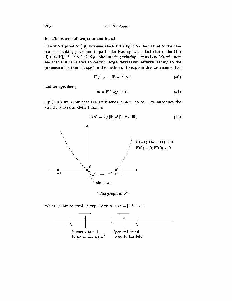
By (1.18) we know that the walk tends Po"a-S- to °°- We introduce thestrictly convex analytic function

F(u) = log(E[p«]), (42)

- l ) and F(l) > 0=0,F'(0) < 0

We are going to create a type of trap in U — [-L , L+]

-L- 0 L+

"general trend "general trendto go to the right" to go to the left"


To quantitatively measure the "trapping effect" taking place in U, we observethat from the martingale property of f(Xn,uj), with

Hz d= inf{& > 0, Xk = z}, for z € TL, (43)

D \ TJ ^ TJ 1•Cl,o; L"0 "^ " L + + l J

with the notation:

f(L+ + l,uf(L+ + l,u

> (l-exp{-,

1 • s-

)-/(l,w)) _ /(0, w)

r-J+R[l,L+]})-II defR+

^ logp(a;,w

— i

f

.)

/(0,w)

' (0 ,w) -

E0<«<LH

II (23)

~/(l,w)/(L+ + l,w)

II (23)

h

(44)

(45)xeJ

for J a non-empty finite subset of TL and \J\ — cardinality of J. In a similarfashion:

fl-ii def

P-!,w[Ho < H_{L-+1)] > (1 - exp{L_ %- ,_! ]})+ . (46)

Let us write .R^ for Ru L], when L > 1. The law of large numbers yieldsthat

RL —^ m = Eflogp] < 0, P-a.s. and in LX (P) . (47)L—>-oo

But large deviations do occur and from Cramer's theory (see [12] or [11]),for e > 0,

P(RL > e) = exp{-L(/(e) + o(l))} as L -> oo, (48)

where for a; € R,

/(a;) = sup {ux - F(u)} (49)

218 A.S. Sznitman

/(•) = oo

slope mine>o e

xm 0

log /9max( > 0)(40)

If we now set for U — [-L , L+]

j(U) = 1 A max(exp{L~iT }, exp{-L+R+})

then with TJJ the exit time from U:

Tu = inf{k > 0, Xk i U},

we see from the strong Markov property that

(50)

(51)

(52)

(with HQ — inf{& > 1, Xk — 0} the hitting time of 0). In particular, ifn"1 :

PoATu > " ] > ( ! - l{U))n > c = e~2 > 0, for n large. (53)

Note that for L~ > T^-, log n, L+, e with L+ e > log n,

<j , R+ > (54)

using independence, (47), (48), for 6 > 0 (small) and large n:

>\ exp{-/(e)L+(l + )}.

We can now optimize e, L+ by looking at:

inf{/(e)L+; eL+ > logn} = inf { ^ x e L + , eL+ > log n\ = iinf ^


and observe that infe>o -*p is the slope of the tangent to /(•) which is passingthrough the origin of the coordinate axes. On the other hand (cf. [12], p. 55):

F(u) — sup(a;n — I(x)) (compare with (49)). (55)

Hence if a — min - ^ (> 0) we see that F(a) — 0. In other words:e > 0 e V ' V '

min —— — s is the positive zero of the function F(-) (by assumption s < 1)e>0 e

(56)

Hence for a suitable K > 0 and any 8 > 0, for large n:

P[Po,w[r[_A:togn>A:iogn] > n] > e"2] > n " ^ 1 + 5 ) . (57)

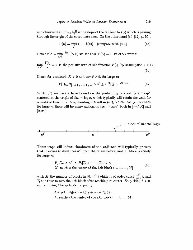
With (57) we have a have bound on the probability of creating a "trap"centered at the origin of size ~ log n, which typically will retain the walk forn units of time. If s' > s, choosing 8 small in (57), we can easily infer thatfor large n, there will be many analogous such "traps" both in [—ns' ,0] and

block of size 2K log n

These traps will induce slowdowns of the walk and will typically preventthat it moves to distances ns from the origin before time n. More preciselyfor large n:

P0[Xn > ns'] < Poin + • • • + TM < n,X, reaches the center of the i.th block i — 1 , . . . , M]

with M the number of blocks in [0,ns ] (which is of order const jf-^), andT{ the time to exit the i.th block after reaching its center. So picking A > 0,and applying Chebychev's inequality

< e x p A n E 0 [ e x p { - X ( T i + ••• + TM)},

X, reaches the center of the i.th block i — 1,..., M].

220 A.S. Sznitman

Using the strong Markov property under Po,w> the independence under P ofenvironments in different blocks, and the stationarity, we find

(57)< exp{An} (1 -

e - 2

+< exp{An-M-^(l-e-^)}

, using 1 — x < e

const n"

if we now choose 6 small, A = \ ns'-s(1+2S)~1

j for n large

_ 1 r}s'-s{l+2S)< exp { - -= e x p ns

Estimating similarly Po[Xn < —ns ], we find that Yln b[|-^n| > ns ] < oo,and from Borel Cantelli's lemma we conclude that:

\X IPo-&.s. lim -—^ = 0, for s' > s — positive zero of F (recall that s < 1),

n ns

(59)(more detailed results can be found in [20]).

We see from (59) that the walk is truly moving sublinearly (in a moreprecise fashion than explained in (19), ii)). The role of traps in thisslowdown is also brought to light, (see also [10]).

2 Higher dimension - traps - conditions (T) anden

We are now turning to higher dimensional random walks in randomenvironment, and we have the following setting:

u(x,e)

x x + e

UJ(X, •) are i.i.d., x


n = Vfd where K € (0, ^ ] is the "ellipticity constant" and (60)

"PK = the collection of (2d)-vectors (j»(e))|e|=1 with

p(e) G [K, 1] for all e and X!|e|=i ^(e) = 1 •

P = product measure on fi, making the u(x, •), a; € Z5d, (61)

i.i.d. with common distribution \i.

Px,wi x £ ^di the canonical law of the Markov chain on 7Ld (62)

with transition probability w(y, e) of jumping to y + e

when located in y.

Px — ]P x PXjUJ, (this is a semi-direct product). The integration (63)

over P restores some translation invariance but typically

destroys the Markov property. One can however represent

the law of the walk under Px as a type of "edge oriented

reinforced random walk", see for instance [14].

In the multi-dimensional context (d > 2), there is no known simple classifi-cation of the asymptotic behavior of the walk in the fashion of (18) and (19)of Lecture 1. Such a classification of possible asymptotic behaviors of thewalk as far as recurrence, transience, ballistic and diffusive behavior of thewalks are concerned, is still very much "under construction". The methodof the environment viewed from the particle has had so far relatively littleimpact on the study of multi-dimensional random walks in random envi-ronment. There are no explicit formulas as (30), and the existence of thedynamic invariant measure Q is only known in a few cases, cf. [4], [23], [25].One substantial difficulty for the mathematical investigation of the modelstems from its genuinely non-reversible character. Until recently few refer-ences dealt with multi-dimensional random walks in random environment(see Kalikow [17], for a sufficient condition for transience, Lawler [25] for acentral limit theorem for driftless walks, and Bricmont-Kupiainen [7] for acentral limit theorem for small isotropic perturbations of the simple randomwalk, when d > 3). However over the last few years there has been progressin the understanding of the situation where the walk has a non-degenerate

222 A.S. Sznitman

limiting velocity thanks to certain conditions which we describe further be-low. For other recent developments see [4], [6], [45], [46], [47], [48]. Wefurther refer to [9], [31], [45] for dependent environments, and to [23], [34],for continuous time and state space.

Traps and spectral considerations

This is maybe one of the most important effects for random walks in randomenvironment. We have already seen the importance of traps in the one-dimensional context when discussing (19) ii) at the end of Lecture 1).

Informally traps are "pockets where the walk can spend a long time witha comparatively high probability". We are now going to define a spectralquantity to measure trapping effects.

For 4> ^ U C 7Ld, we define

u(x,e)f(x + e), (64)= l

in other words RYu is the transition kernel of the walk killed when exitingU. I f < w = ( i ^ > , n > l

R%u f(x) = Ex>ul[f(Xn), TV > n], with Tv = inf{n > 0, Xn £ U},(65)

the exit time from U.

Observe thatll#n,JI°o,oo = sup PXtj[Tu > n],

X

and by sub-multiplicativity (||i^+m!J|oo,oo < W.JIoo.oo K,J|oo,oo) wecan define

= I im- i log |K,J|oo,oo G [0,oo]

" (66)= SUP-- log ||i^J|oo,oo-

71

In other words e~û^ is the spectral radius of RY^ acting on L°°(U) (cf.Rudin [33], p. 234-325). The number Aw(f7) quantifies the strength of thetrap created by LO in U. The smaller X,j(U) the stronger the trappingeffect.

One should however be aware that we are dealing with a quite non-self adjoint situation, see also [5] p. 32, 33, and Aw(f7) offers a quantitative


lower bound on ||-R^<J| 00,00 (namely as follows from the second line of (66),

1100,00 > e~nXu>(u\ n > 1), but in general does not provide a quantita-tive upper bound on ||-R^cJ|oo,oo — PXjU1 [ > n]. A trivial example tofeel the problem is:

U — {0 , . . . , n} (depending on n), d — 1, LO: "jump to the right"

1 1 1 1 1 1 1

H V0 n

then \u(U) — 00, but PO,U[TJJ > n] — 1 which is not dominated by e nX"(u).The problem comes from the fact that ^(U) only measures an asymp-totic ability for survival. However the above remark on the non-quantitativecharacter of Aw(f7) should be taken with a grain of salt, as we will explainfurther below, (cf. (75)).

Before expanding on this last remark, let us first discuss the fact thatthere is a classification of the strength of possible traps which can becreated by a random environment. To this end we consider the localdrift at x in the environment ui:

d(x,u) — ^ uix, e)e — EXjUJ[Xi - Xo],|e|=l

(67)

and introduce

KQ — the convex hull of the support of the law of d(0, ui) under P . (68)

"An example of KQ in the plain nestling case"

224 A.S. Sznitman

The position of 0 with respect to KQ plays a crucial role. Namely (cf. The-orem 1.2 in [40]), with BL — B(0,L) D 7Ld, and ci,C2 two positive constantsdepending on d and the single site distribution \i\

• in the "non-nestling case" (i.e. 0 ^ KQ):

i) P-a.s., c2 < \U{BL) < CI, L > 1,

• in the "marginal nestling case":

ii) P-a.s., H < AW(£L), L > 1, and P [ A W ( £ L ) < ^ ] > 0,L

• in the "plain nestling case":

iii) P-a.s., e"C2L < \W{BL), L > 1, and P[AW(£L) < e"ClL] > 0,L large.(69)

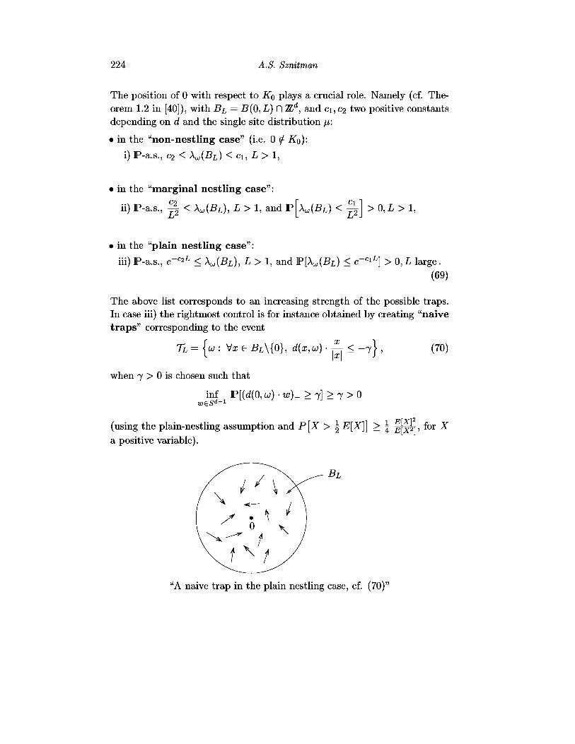
The above list corresponds to an increasing strength of the possible traps.In case iii) the rightmost control is for instance obtained by creating "naivetraps" corresponding to the event

TL = {w : Vx € BL\{0}, d(x,«,) • - < - 7 } , (70)

when 7 > 0 is chosen such that

inf P[(d(0, w) -w)-> 7] > 7 > 0S41

(using the plain-nestling assumption and P[X > ^ E[X]] > \ § | w , for X

a positive variable).

"A naive trap in the plain nestling case, cf. (70)"


As was alluded to above, the number \W{U) can be used to produce quanti-tative lower bounds (i.e. non-exclusively asymptotic) on the probability ofsurviving in U. For instance

Lemma 2.1.

For L > 0, n > 0, P0[ |^n| < 2L] > P0[TB2L > n] >-?— E[exp{-nAa;(SL)}]\£>L\

(71)

translation

Proof. For x £ BL, P0[TB2L > n] > P0[TBL.X > n] i nvai:ance PX[TBL > n], sothat summing over x € Bi:

P0[TB2L > n] > — Y^ P*[TBL > n] = ^ E [ £ PX^[TBL > n]]

(66) second line \

D

There is a-priori no quantitative upper-bounds in general. One can how-ever introduce for <f> ^ U C 7Ld,

, where iw(f7) = inf < n > 0, ||-Rn,wlloo,oo < ; ? £ { 1 , - - ,00} ,

/* \yields quantitative upper bound on decay of

(72)

From the inequality e~Xu>Wtu>^ < | , when tu(U) < 00, we infer

K,(u). (73)

Of course these numbers can be very different, for instance in the examplegiven above (67), Aw(?7) = oo, but Aw(?7) = %& !!!

However one can devise an upper bound for Aw(f7) in terms of Aand when Aw(f7)|f7| is small then Aw(f7) is small as well:

226 A.S. Sznitman

Lemma 2.2. (<f> Û finite, u g f i j

~ 2there exist XQ € U, such that PXo u,[HXo > Tu] <

(HXo — inf{n > l,Xn — XQ} the hitting time of

^ (75)

or equivalently:

Proof. For some x\ € U, \ < PXI,U[TJJ > tw(U)] and by a classical Markovchain calculation

> Ttr] mf Ptf>w[fftf >

and (74) follows. Then observe that for y € f7

fe ] n < Py>w[TD- > n] <

(this has very much the same flavor as (52)), and hence taking the n-th rootand letting n tend to infinity:

P%uj[Hy <Tu] = l - Py^Hy > TV]. (76)

If we now choose y — XQ, we obtain our claim. •

Observe that (75) offers some quantitative upper-bound on the decay of||.R^J|oo,oo (via an upper-bound on tw{U)) from the knowledge of XW{U) and\U\. This is the grain of salt alluded to after the example above (67).

We now turn to the discussion of ballistic walks, and begin with thedefinition of conditions which have far reaching consequences.


Conditions (T) and (T'):

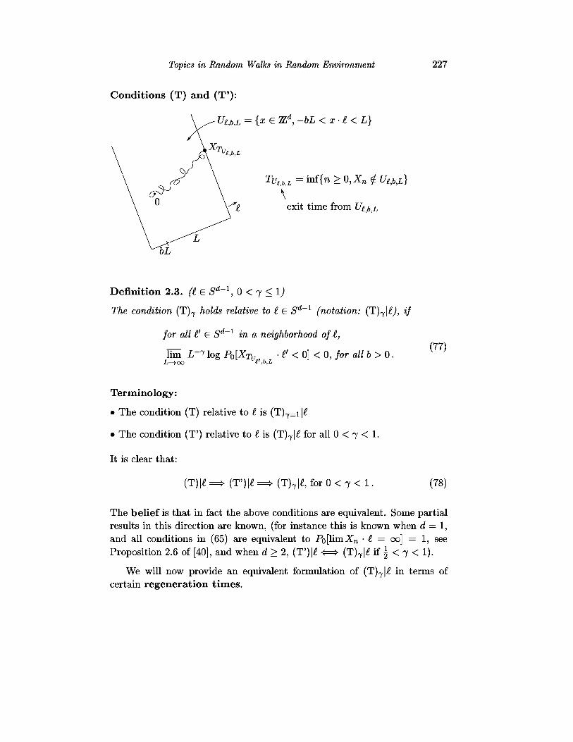
• Ue,b,L — { x e /L , - o h < x - i < L )

TUtbL=wf{n>0,Xn$Utjb,L}

\exit time from

Definition 2.3. (I € S*'1, 0 < 7 < 1)

The condition (T)7 holds relative to £ €. 5 d - 1 (notation: (T)7|£^; if

for all £' € 5 d - 1 in a neighborhood of I,

Em L-T log Pot^r. • £' < 0] < 0; for all b > 0.(77)

Terminology:

• The condition (T) relative to I is (T)7=i \£

• The condition (T') relative to I is (T)7|£ for all 0 < 7 < 1.

It is clear that:

(T)|£ => (T)\l => (T)7|£, for 0 < 7 < 1 • (78)

The belief is that in fact the above conditions are equivalent. Some partialresults in this direction are known, (for instance this is known when d — 1,and all conditions in (65) are equivalent to Po[lim^n • •£ = 00] = 1, seeProposition 2.6 of [40], and when d > 2, (T)\l <^> (T)7|£ if \ < 7 < 1).

We will now provide an equivalent formulation of (T)7|£ in terms ofcertain regeneration times.

228 A.S. Sznitman

Notation: for I G S*"1, u € U,

T!. = infln > 0, Xn • I > u\, T* = inf{n > 0, Xn • I < u\

(79)Dl = inf {n >0,Xn-i<X0-i}.

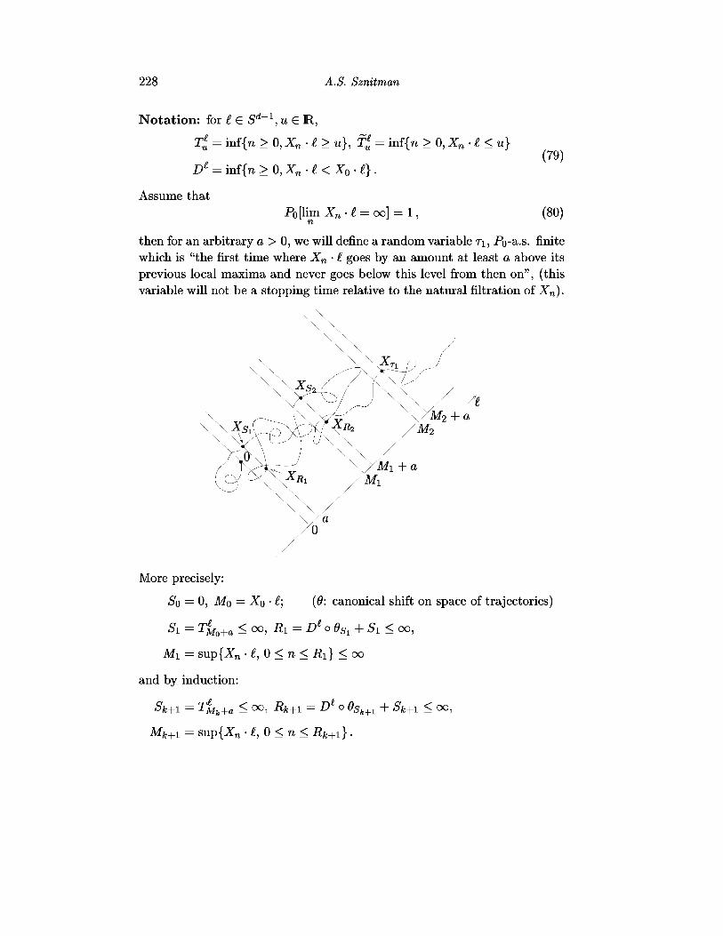
Assume thatP0[lim Xn • £ = oo] = 1 , (80)

n

then for an arbitrary a > 0, we will define a random variable TI, Po~a-S- finitewhich is "the first time where Xn • t goes by an amount at least a above itsprevious local maxima and never goes below this level from then on", (thisvariable will not be a stopping time relative to the natural filtration of Xn).

WV \/M2 + a

/ a"0

More precisely:

SQ — 0, Mo = XQ • £; (0: canonical shift on space of trajectories)

Si = Tffo+a < oo, fli = ^ o 0Sl + Si < oo,

Mi = sup{Xn • £, 0 < n < Ri} < oo

and by induction:

Sfe+i = Tfth+a < oo, i?fe+i = D* o 0S/fe+1 + Sk+1 < oo,

Mfe+i = sup{Xn • I, 0 < n <


With (80) it is not hard to show (see Proposition 1.2 of [43])

P0[De — oo] > 0, and Po"a-S- K < oo, provided

K — inf{& > 1, Sk < oo and Rk — oo}.

We can then define the regeneration time

T\ = OK • \P")

As we will now explain the conditions (T)7|£ can be rephrased in terms ofan estimate on the size of the trajectory Xk, 0 < k < T\, (cf. [41], Theorem1.1).

T h e o r e m 2.4. (I € S"*"1, 0 < 7 < l ; a > 0 ;

One has the equivalence

ii) (80) and for some c > 0, Eo[exp{c sup |Xfc|7}] < oo . ^ '<fe<

Sketch of proof: For simplicity we assume 7 = 1 .

i) ^^- ii): We choose an orthonormal basis (fi)i<i<d of R^ with / i = I, andfor each 2 0, £i,+ -fi>0, ii,- • fi < 0, a n d (84)

iim L~l logP0[XTu • g < 0] < 0, for g = i, ii&, £ and 6 > 0.

(85)

We can now pick numbers ai,± > 0 large enough so that

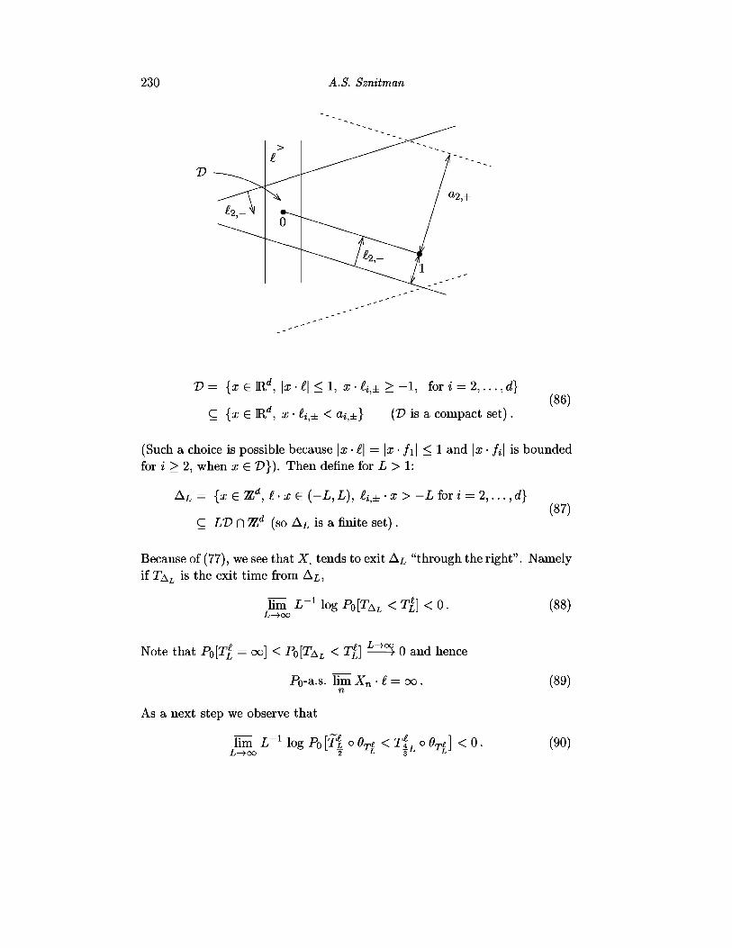
230 A.S. Sznitman

V

V= {x G Ud, \x • £\ < 1, x • £,± > - 1 , for i = 2 , . . . , d}

C {a; G Rd , a; • £i;± < aj, is a compact set).(86)

(Such a choice is possible because \x • £\ — \x • / i | < 1 and \x • fi\ is boundedfor i > 2, when x G 2?}). Then define for L > 1:

AL = {a; G Kd, £ • a; G ( -L, L), £ i j± • a; > - L for i = 2 , . . . , d}

C LT>n7Ld (so AL is a finite set).(87)

Because of (77), we see that X, tends to exit A^ "through the right". Namelyif TAL is the exit time from A^,

(88)lim L~l log P0[TAL <T[}<0.L-KX>

Note that P0[T[ = oo] < PQ[TAL < T[] ^ ^ 0 and hence

Po-a.s. lim Xn • £ = oo . (89)n

As a next step we observe that

lim L" 1 log Po \T{ o6Ti < T | , o 9Te] < 0. (90)


Indeed:

P0[T{oOTi < Ti o9TA < P0[TAL < T[]+P0[T{ O 9Ti < Ti o 9Ti,TAL =

2 L 3 ^ 2 ^ 3 ^

using translation invariance and the strong Markov property

< P0[TAL < Ti] + |0AL| PQ[f\ < Ti]2 3

and (90) follows from (88).Applying Borel-Cantelli's lemma:

P0-a.s. for large integer L,T{ <T[ + T{O 0Ti . (91)ZL 2 L

So on a set of full Po-measure we can construct L& € N f oo, with Lfe+i =[| Lk] and T/fc+i < T^+T^ o0 T | , for A; > 0. This implies that (80) holds,

i.e.Po-a.s. lim Xn • £ — oo.

n

(as noted above (81) follows). For the next lemma we use the notation

M = sup{Xfe -e-X0'£, 0 < k < D1-}. (92)

Lemma 2.5. (Assuming (80)^

Under PQ, XTl • t is stochastically dominated by a + 1 + Gj, whereGo — 0 and Gn «s the sum of i.i.d. variables Mi,..., Mn distributedlike M + a + 1 under PQ[ -\D* < oo] and J «s an independent geometricvariable with parameter PQ[D^ < oo].

(93)

Sketch of proof of Lemma 2.5: F(-) > 0, non-decreasing, then

EO[F(XT1 • 1)] ( 8 i } ^ E0[F(XSk • I), Sk < oo, Dl o 0S/fe = oo]

[ jk ), Sk < oo, XS/fe = x] Px,w \Dl = oo] ]fe>l jjgzd " v ' " v '

a(ui(y,-);i-y<i-x)—meas. a(ui(y,-);i-y>i-x)—meas.

independence v1 IT FfiVV ^\ « / ^ l P f n < ™1

(94)

232 A.S. Sznitman

Then for k > 2:

E0[F(XSk • l),Sk < oo] < ^ [ ^ ( M f e . ! + a + 1), 5fe_i < o o , ^ o 0 ^ < oo]

i + a + 1), 5fe_i < oo, X ^ = x, D1 o 0Sjk_1 < oo]

and arguing as above

< £0 ^ P ^ • i + M), Sk-i < oo] P0[D* < oo]by induction f^/u -,\

< £ o x ^ ( }[F(a + 1 + Mi • • • + Mfc_i)] P o [ ^ < oop" 1 )(95)

and one checks directly that (95) also holds when k — 1. Inserting this in(94) we find EQ[F(XT1 • £)] < £?[F(a + 1 + Gj)], and our claim follows. D

As a result for c > 0,E0[exp{cXT1 • £}]

< e<a+VPv[Dl = oo] S

(96)and if we show that for some c' > 0, £ro[ec'M|.E^ < oo] < oo, it will followthat for some small c > 0,

E0[exp{cXTl • I}] < oo. (97)

To finish proving (97), note that for large k

and E(j[ec M\Di < oo] < oo for some c' > 0, easily follows and (97) as well.

We can now finish the proof of i) ==$- ii). We pick r > 0 such thatV C B(0,r) (see (86)) and hence AL C B(0,rL). Then for large u > 0:

sup |Xn | > u] < P0[TA u < n ] • i): Under (80), one can in fact use T\ as a regeneration time and seethat under PQ, XTl+. — Xn has same distribution as X. under PQ[ -\D^ — oo]and then iterate:

T2 = T-\_{X) + Ti(XT1+. — XT1) (— oo, if T\ — oo), and by induction

rk+1 = Tl(X) + Tk(XTl+. -Xn), (see [43]).

One obtains the crucial renewal property:

under Po, (XTlA.), (X(Tl+.)AT2 - XT1),..., (X(T/fe+.)AT/fe+1 - Xn) (99)

are independent and except for the first variable distributed like (XTlA.) un-derP0[-\Di = OO].

Incidentally note that Tk+i — Tk is indistinguishable from a measurablefunction of((X(T/fe+.)AT — XTft), (namely the first time when the trajectory remainsfrom then on constant).

Prom the integrability of supfe<Tl \Xk\ under P Q H - ^ — °°] a n d the lawof large numbers, we easily deduce that

P0-a.s., \Xn\ -> oo and ^ - , v=\X\

and of course v • t > 0.

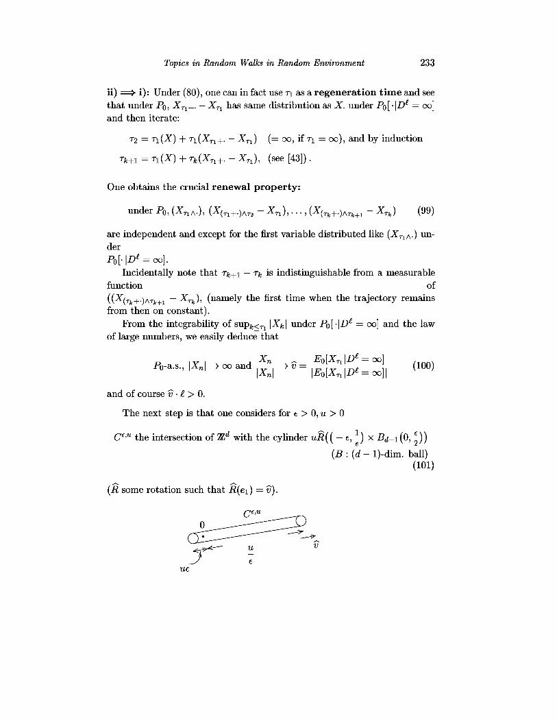
The next step is that one considers for e > 0, u > 0

C£'u the intersection of TLd with the cylinder uR(( - e, ) x Bd-i (0, | ) )

(B:(d- l)-dim. ball)(101)

(R some rotation such that R(ei) — d).

Ce,u

0

234 A.S. Sznitman

One has with the help of the exponential bound in ii), the renewal property(99), and a Cramer-type large deviation control,

Ihn" n"1 log Po \TCcu -0O e

(see Lemma 1.3 of [41] or Lemma 2.3 of [40]). But since v-l > 0, by makinge > 0 small in (101), i) follows immediately. •

Remarks: 1) Under (T)7|£

PQ-SL.S., \Xn\ —> oo and " —> v € Sd~l deterministic, and (103)

(T)7 \£' holds if and only if v • £' > 0. (104)

2) Note that in i) we have only used the fact that

lim L" 7 log Po [XTu • t < 0] < 0, for b > 0,Jj £ ,b,L

for finitely many £' such that V in (86) is a compact subset of

Open problem: Is (T)7|£ equivalent to

lim L-T logPo[XTutibiL • £ < 0], for b > 0,

(in other words: only £' — t is needed)? •

As we will see (83) i) and (83) ii) have different merits. On onehand (83) i) will be more appropriate to derive sufficient criteria for checking(T)7 or analyzing possible equivalences of these conditions, cf. below (78).On the other hand (83) ii) together with the renewal property (99), will bemore handy to derive consequences of (T) or (T') on the asymptotic behaviorof the walk.

3 Checking conditions (T) and (T')

We are now going to discuss various ways of checking conditions (T)and (T').

Conditions (T) and (T'), cf. (77), require a control on the large L asymp-totics of the exit distribution of X. from slabs U^L, under PQ. This is not


a-priori an easy task, since in particular the walk X. under PQ does nothave the Markov property. We will now discuss two ways of handling thisdifficulty.

Kalikow's approach: The idea is to reintroduce a Markovian character tothe problem by introducing certain auxiliary Markov chains, following[17]. Namely, for U £ TLd a connected subset containing 0, one defines aMarkov chain with state space U U dU and transition kernel:

&, x -f a —{0, x, w)J (105)

Pu(x, x) = 1, when x G dU (d= {z G f/c, 3a/ G tf, |z - z'| = 1}),

here we use the notation "gui'i '•>w) f° r * n e function:

Tugu(x, y, u) = EXjU1\j2 l{Xn = y}] , (106)

0

which is a slight modification (on dU) of the Green function, cf. (164). Wedenote by Px>u the law of the canonical Markov chain starting at x G UUdU,corresponding to the transition kernel (105). The interest of this notionintroduced by Kalikow is

Lemma 3 .1. / / PQ,U[TU < oo] = 1, then Po[Tu < oo] = 1 and XTu hassame law under Po,J7 and Po-

(This "reduces" the calculation of the exit distribution of X from Uunder Po, to a Markovian problem).

Proof, (the i.i.d. character of P , plays no role).

For x G U U dU, u G fi, we deduce from the simple Markov property thefollowing equation:

gu(0, x, w) = S0jX+^2 gu(0, y, w) w(y, x-y), with u(x, z) = 0, when \z\ ^ I

Integrating over P , we obtain

Egtr(0, s, w)] = ( o + ^ Egtr(O, y, w) u(y, x - y)]

(107))

236 A.S. Sznitman

Moreover:

gu(x) = %,v [ £ l{*fc = x}\, x € U U 8U, (108)fe=0

is the minimal non-negative solution of the equation:

f(x) = 60,x + £) f(v) ?u(y, x-y), f:UUdUÛ+, (109)yeu

(one observes that du,n(x) = -E'o,J7[X] =o™ H^fe — x}] satisfies:

9U,n+l{x) = ^0,x + Y 3U,n{v) PuiVi x ~ V) >

and by induction one also sees that / > ~gu,n, s o that letting n —> oo, / >follows).

Hence from (107), we find

gu(x) <E\gu(0,x,u)], xtUUdU. (110)

Moreover, for x € dU,

gu(x) = P0,u[Tu < oo, XTV = x], E,\gu(0,x,u)] = Po[Tu < cx>,XTu = x]

and by assumption YlxedU §u(x) — > s o that from (110) we obtain

gu(x) = -E\(ju(0,x,u>)]; x £ 3U.

(It is also not hard to see that this equality in fact holds for x € U and as aby-product of summing over x in U, one finds that EOtu[Tu] — EQ[TU]). •

One way to make use of this is to introduce the auxiliary local drift:

Mx) = ExpiXi -X0],x€UUdU, (111)

and introduce the Kalikow condition relative to t € 5 d~ 1 , (Notation(K)\£):

inf du(x) -1 = e(l, n) > 0. (112)U£U

As we now see it implies condition (T) (and hence (T')).

Proposition 3.2. (£ G Sd~1,d> 1)

(K)\£^(T)\£ (113)


Proof. We can find 7 > 0, such that for 9 G [0,1], \u\ < 1,

\e-0u - 1 + 9u\ < j92 .

Hence for n > 0, U as in (105): with (^n)n>0 the filtration of X., x €

W V ^^( n G U}

EXn>u[exp{-9(X1 - Xo) • £}]), Px,u-&.s..

Because of (112), for 0 < 9 < 9(e), and y G U:

Ey,u[e-9{Xl-XoH} < 1 - 9dv(y) -£ + J92<1. (114)

Hence we have:

e-9(e)xn-i^ n > o, is an (J>i)-supermartingale under PXJJ . (H5)

Prom the stopping theorem we immediately obtain:

iim L" 1 log Po \XTu • £ < 0l < -W(e) < 0 (116)

(recall the notations above (77)).

Note also that (K)\£ =$• (K)\£' for all £' in some neighborhood of £, sothat applying (116) to such £', we obtain (T)\£. •

One can then provide conditions (much more explicit than (112) whichimply (K)\£ and hence (T)|£.

Proposi t ion 3.3. (£ G 5 d" 1 ,d > 1

J/E[(d(0,w) •£)+] > - E[(d(0,w) •£)_], i/ien (K)\£ and hence (T)\£ hold.(117)

(K is defined in (60)^.

Proof. For U as in (105), and x G [/", by a standard Markov chain calculation:

9u{ ' 'w ) = P [ ^ > r F ] E|e|=l

238 A.S. Sznitman

(Hx: entrance time, Hx: hitting time). Nowl P F P[

(0,x,u)] L £ u(x,e)Px+e,UJ[Hx>Tu]|e|=l

< 2V]

i

J

E[<ft/(O, x, u)] Lmax|e|=l

and using independence

(x,1 . .

(d(x,

Ee|=l

(118)

and our claim follows. D

With the above proposition we already have a variety of concrete situa-tions where (T)|£ holds. We will now discuss another approach to check (T')(and possibly (T) but this is open for the time being).

Effective Criterion:

d+B

L + 2sV^L-2

Notations: £ € Sd~\ R is a rotation of Ud with R(ei) = £, L > 2, L > 0,

£ = fl((-(L - 2),L + 2) x ( -L,L)^ 1) n ^ : a box

d+B = dB D {x £ 7ld, £ • x > L + 2, \R(ei) -x\<L, for each i > 2}


One has an equivalent characterization of (T')|£ in terms of moments of thePB'S. Note that pB has some flavor of p in (17).

Theorem 3.4. (I G S*-1)

(T')|£ is equivalent to

i y i d ~ 1 ) } 1 (120)

where B in the above infimum varies over the collection of boxes B corre-sponding to an arbitrary rotation R, L > C2(d), and ZVd < L < L3, andci(d), C2(d) are dimension dependent constants bigger than one.

Remarks: 1) The interest of the theorem comes from the infimum in (120)and the effective character of (120). In other words it suffices to find a boxB and an a for which:

to know that (T')|£ holds. If this is the case the infimum in (120) is in fact0.

2) The condition (120) has some flavor of the condition E[p] < 1, in (19),in the one-dimensional case, which ensures the ballistic behavior of thewalk. In particular (120) involves a small denominator question (namelyPOJUJ[XTB G d+B] may be small), which is related to the possibility of atyp-ical exit probabilities of the walk, a phenomenon which is related to theoccurrence of traps in the medium. •

Some comments on the proof: (for more details see Section 2 of [41])

• (120) => (T)\t

The idea is to define a sequence of boxes B^, which grow, but not too fast,and tend to look like "infinite slabs", and use a control on a moment of pBk

to obtain a control on a moment of PBk+1- This is a "renormalizationmethod", where a certain induction hypothesis concerning the smallnessof certain moments of psk is propelled "from one scale to the next scale".Specifically one defines for a suitable no G (0,1]:

(const(d)\k k(k i) j (Lk\3

T , .Lk - I ) 8 2 L0 ) Lk - I — I Lo (121)

240 A.S. Sznitman

, -* ,and one controls for a suitable ao € (0,1], E[/9g°2 "], (one shows that

c(d) L^Lk E [tfg-h] < K"° i* , (122)

by induction). Note that

and from (122) one can prove that for some c > 0,

iim L~l exp{c(log L) 5 } log P o [ ^ & L< 0] < 0, for all b > 0 . (123)

Then by a perturbat ion argument one shows that a similar control as (120)holds for all small enough perturbations £' of I and one obtains for (! in aneighborhood of t controls like (123), which in fact is more than enough toshow (T')|£.

In fact we explain (T)7 |£ =^- (120), when \ < 7 < 1, which of course impliesthe claim.

We choose the box B of the form:

L large, L — AL, where A is some constant (depending on {T,I)

R any rotation with R(ei) — £.

C£>L

(124)

L = AL

L-2 =—= L + 2


If C6'1* is defined as in (88), choosing e > 0 small we have for all large L:

PQ,W [Tl = TCC,L] < POAXTB e d+B]. (125)e

Hence for a G (0,1] and c > 0:

nP%\ < nP%,P»AXTB € d+B] > e~cL1] + TE[P%,P0,U1[XTB G d+B] < e~cL

using the fact that E[Za] < E[Z]a, for Z > 0, since 0 < a < 1,

< eacL7 P 0 [ ^ r s £ d+B]a

using ellipticity

(125) K-c(d)aL

< eacL1 Po [Tf > TCc,L]a + 3 ^ Po [Tl > TCC,L] .

(126)

Now under (T7)|£, the control corresponding to (89) is:

lim n" 7 log P0[TCe,n < i f ] < 0. (127)

Hence choosing a — L~2 and c sufficiently small in (126), we obtain:

EmL-fr-^logEIpjf *] < 0, (128)

and this is more than enough to prove (120). •

We see that (120) implies already a condition which formally looks strongerthan (T)\£, cf. (123), (77), (78). One has in fact the

Open problem: Are all (T)7|£, for 0 < 7 < 1, equivalent? (And of coursethen equivalent to (120)).

The effective criterion is interesting from different perspectives. Onthe one hand it is a theoretical tool: for instance we have seen thanks to(121) that

for \ < 7 < 1, I (E S*-1, (Ty)\£ and (T)\£ are equivalent. (129)

One can also rather easily check with the help of (120) that the set of singlesite distributions fj, on VK (we have P = /i®z ) for which (T')|£ holds isopen for the weak topology (i.e. (T')|£ is stable under small perturbationsof the distribution). This is not so clear from the definition of (T')|£ in (77)

242 A.S. Sznitman

or even from (83), on the other hand the continuity of /J, —> E[/9^] for B,a as in (120), is straightforward. Indeed, PQ^[XTB G 8+B,TB < M], forM —> oo, are polynomials with positive coefficients in the variables UJ(X, e),x G .B, |e| = 1, which uniformly in w converge to PQJW[XTB G 0+-B] which isuniformly positive by ellipticity. This continuity and (120) now implies theclaim.

On the other hand the effective criterion as we later will see is also aninstrument to construct examples where (T') holds.

4 Asymptotic behavior under (T) and (T')

We will now discuss some consequences of conditions (T) and (T').This will explain the interest of these conditions.

Law of large numbers and central limit theorem:

The full strength of conditions (T) or (T') appears when d > 2. Whend — 1, (T)7|£ is equivalent to Po[lim^n ••£ = oo] = 1, for any 0 < 7 < 1, andI — ±1 , cf. [41]. Hence in the one-dimensional context, all these conditionsare equivalent to a transient behavior of the walk in the direction £, and aswe have seen in (18), (19) ii) this may happen without a ballistic behaviorof the walk. The multi-dimensional case turns out to be different.

Theorem 4.1. (d > 2, I G Sd~l, under (T)\l)

Po-a.s., — —> v deterministic with v • £ > 0, (130)

Bn = X{.n] -[•»]» converges in law on the space D(B+,B*) (131)

of right continuous Mr-valued trajectories

with left limits, to a Brownian motion with

non-degenerate covariance matrix A.

Sketch of Proof: With the help of the renewal property (99), the law of largenumbers follows in essence from the estimate:

= oo] < oo, (132)

and as a matter of fact

_ E0[XT1\D* = oo]V


In a similar vein the functional central limit theorem follows from the esti-mate

E0[rf\De = oo] <oo , (134)

and the limiting covariance is then:

A ~ E0[T1\D* = oo] •

For details see [43] and also [39]. In some sense proving (130) and (131) boilsdown to controlling the tail of T\. We discuss these estimates further below.•

Open problem: When d > 2, are (T') or (T) characteristic of ballisticbehavior: does a strong law of large numbers with non-vanishing limitingvelocity imply (T) (and of course (T'))? More generally, does (80) imply

Tail estimates on the regeneration timesAs we now see under (T') (and of course (T)), n has finite moments ofarbitrary order under PQ, when d > 2. This is quite different of the one-dimensional situation, and this feature should be viewed as a reflection ofthe weakening effect of traps as dimension increases.

Theorem 4.2. (d > 2, under (T')|£, a > 0) (a enters the definition of T\above (81),)

Po[n > u] < exp{-(logn)a} ; for large u,2d ( 1 3 6 )

when a < -—- (<— number bigger than 11) .

Let us mention that in the plain nestling situation, under the above assump-tions, we can use the naive traps discussed in (70) and obtain the lowerbound

Po[n >u]> exp{-c(logn)d}, for large u. (137)

Essentially one chooses L — K logn, with K large and one constrains thewalk to remain in Bi up to time [u] + 2 and be in 0 at time [u] + 1 or[u] + 2, depending on the parity of [u], which happens with a not too smallprobability > exp{—const(logn)}, uniformly for w in the trapping event 71of (70), if K is chosen large. On the other hand P[7L] > exp{—const Ld} inthe plain nestling situation, and (137) easily follows.

244 A.S. Sznitman

Sketch of proof of (136): We will explain how certain estimates on the occur-rence of atypical quenched exit dis t r ibut ions of the walk from certainasymmetric large slabs are crucial in the derivation of (136). We need somenotations:

G [0,1], and Upj, = {x£7Zd,x-l£ (-L^, (138)

We want to control the P-probability that Po,w [XTV • I > 0] is atypically

small, (this should not be confused with (77)!).

naive trapof size K L?

Plain nestling situation

"An event ensuring that PQui[XTu • t > 0] < e~cL0v~cL0v

The crucial role of such controls in the derivation of (136) comes from the

Proposition 4.3. (d > 2, (T)\l)

Assume (3 G (0,1) is such that for all c > 0,

1lim

L—>-oo L8,L

£ > 0] < e~cL ] < 0, then

lim (logn) ^ log P0[n > u] <0, for any ( < - ,u—>-oo p

(139)

(140)

(when (T)\£ holds one can choose ( — \).


Proof. We choose some ( as in (140).

We define An = 8\ogu and L(u) — A(n)? ^> A(n), where 8 > 0 is smalland chosen below (143). Then for large u,

Po[n >u}< P0[TI > u,TC L ( U ) < n ] + Po[TcL(u) > u] , (141)

with the notation Cr — (—§, | ) d . Since TcL{u) < n forces sup0<fe<Tl \Xk\ >

~Y^-, applying Chebychev's inequality and (83) ii) with 7 close to 1, so that

% > C> w e obtain for large u:

< exp{-(logn)c} + Po[TcL(u) > u] .

We thus only need to estimate the last term. In the notation of (72) wehave:

PO[TCL(U) >u]< EIPO^TC^ > u], tw{CL{u)) <

Markovproperty

(logu)'

[ u -1 property /1

(logn)? J (74) V2(142)

P[for some x0 G CL{u), Px^[HXo > TCL(U)] < - |CL ( u ) | ( togu)?].

On the event inside the above probability, for x ^ XQ

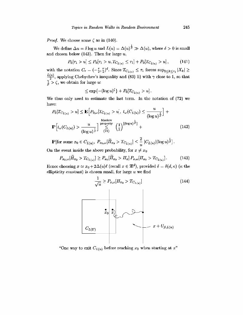
PX0AHX0 > TCL(U)] > PX0[HX0 > Hx] PXfi,[HX0 > TCL(U)] . (143)

Hence choosing x ~ xo + 2A(n)£ (recall x G d ) , provided ^ = ^(d, K) (K theellipticity constant) is chosen small, for large u we find

' ~* \H >Tn 1 (144)1 *

+

"One way to exit CL(U) before reaching XQ when starting at x"

246 A.S. Sznitman

Note that - ^ = e " ^ A ( u ) = e"^L ( u ) ' 3 , so that from (139), (142) and trans-lation invariance, for large u:

u](139)

< exp{—const L(u)}.

Together with (141), the claim (140) follows.•

In view of the above Proposition, the heart of the matter in the proof of(136) comes from the crucial estimate:

Theorem 4.4. (d > 2, (T)\i)

For c > 0, /? G (0,1),

e~cL0[XTu0 L4 > 0] < e~cL0\ <0fora< [ ^(145)

(one can replace Po,w[^7V -^ > 0] by \U(BL) in (145), see Proposition 4.7of [40], where this is shown under (T), but also holds under (T')^

a = d/3

a — 2 ,

(lower bound in the plain nestling case,see below (138);

L (general upper bound, see (145),)

d+l

For details about the proof of (145), we refer to Lemma 3.2, 3.3 in [41].


v limiting velocity

o — - + e 4— small

+ 1 - X

The idea of the proof of (145) for \ < (3 < 1, and a < d(2(3 - 1), is toconstruct within distance ~ L@ of 0 a number of potential escape routes forthe walk along thin tubes in the direction of the limiting velocity v. Thesetubes are made by piling up smaller boxes of height Lx and base of size Lx^°with flo close to ^. One uses a renormalization step showing that if a certainestimate holds on the smaller boxes then the probability that none of theescape routes along the tubes yields a probability at least e~cL to exit UptLthrough the "right side" is smaller than exp{—L^2^"1)"^} (77 small) for Llarge.

The case a < a® = ^ - < 1, follows rather straightforwardly from theprevious bound. One defines U — {x € 7Ld,x-l € (—ifl, L7)}, with 7 = ao +e < 1, (e small). One notes that Po^[XTu-£ > 0] = POjU,[XTu L-l> 0]+rem.,where rem. = PQ>W[XTV • £ > 0, XTV • £ < 0]. But from Chebychev'sinequality and the control on M below (97), for large L, P[rem. > e~cL ] <

g_L«o j j e n c e o n e o n iy n e e ( j s to estimate PfPo^t^r^ •£ > 0] < e~% L ], whenL is large. But the claim follows from the previous bound and the identityU = UiL1, with \ < £ < 1, (e is small). •

This completes our sketch of the proof of (136). •Open problems:

Can one pick a — dfi in (145)?

Can one have an upper bound in (136) of comparable order to the lowerbound (137)?

248 A.S. Sznitman

Both issues are closely related (cf. Proposition 4.3), and the implicitquestion at hand is "whether there is anything truly better than naive traps",to make T\ big or to provoke an atypical exit distribution from slabs like C^,L?Note that some traps may not be massive like the naive traps of (70), butdiffuse, and functioning for instance like a fountain which works both withthe help and against gravity.

a diffuse trap"like a fountain"

Slowdowns: We now turn to large deviations of ^ under PQ orAn interesting effect takes place in the nestling case when we assume(T) or (T). First of all (cf. Theorem 4.1 of [40])

, v — limiting velocity

"The segment [0, v] is critical in the nestling case"

Theorem 4.5. (d > 2, under (T)\£)

If O is a neighborhood of [0, v], then

Em" - logP0[— i (146)

In the non-nestling case, (146) holds for O a neighborhood of v. In thenestling case on the other hand, for U an open set with U D [0, v] 0,

lim - logPof—n n in

= 0. (147)


Open problem: Prove a large deviation principle for ^ under Po, with arate function necessarily vanishing on [0,v], in the nestling case.

On the other hand under PQ,U, one has in the nestling situation a largedeviation principle due to Zerner [46].

Theorem 4.6. (nestling case)

For P-a.e. w, ^ satisfies a large deviation principle on Ptd under PojW withspeed n and deterministic continuous convex rate function /(•) which is finiteon {x € Rd , \xi\-\ h \x,i\ < 1} and infinite outside. In addition when (T)holds:

{J( . )=O} = [O,t;]. (148)

We thus see in view of (147) and (148) the critical nature of largedeviations of ^ in the neighborhood of [0,v]. Such large deviations can beviewed as slowdowns of the walk, where the general direction of the motionis kept unchanged but the pace is slower.

To begin the discussion of this finer effect we start with the case ofwalks which are neutral or biased to the right, where the theory isquite successful and slowdowns are linked to another well-known effect. Thewalks are now such that for some 8 > 0:

(149)

ii) P[{w(0, .) = -}]>0, P[{d(0,U) • ei > 8}] > 0.

Note that in view of (117), (T)|ei is satisfied. The description of the criticallarge deviations comes in the next theorem:

Theorem 4.7. (d > I, under (149)^

//Mn[0,ti] ^4>, U open

lim n~d+2 logP0 [— G w] > -oo . (150)n L n J

If O is a neighborhood of v:

Ihn" 7 1 - ^ 2 k ) g P o [ ^ <td\ < 0 . (151)n L n J

Moreover P-a.s., forll and O as above similar estimate hold under Po,w with

n~dh replaced by

250 A.S. Sznitman

The above asymptotics are strongly reminiscent both in the annealedand quenched situation to what happens in the problem of the "long timesurvival of Brownian motion among Poissonian obstacles", see [37], Chapter4 §5.

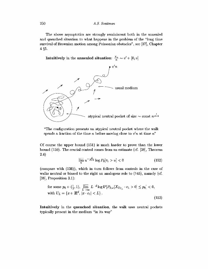
Intuitively in the annealed situation: ^ ~ v' G [0, v]

usual medium

atypical neutral pocket of size ~ const nd+2

"The configuration presents an atypical neutral pocket where the walkspends a fraction of the time n before moving close to v'n at time n"

Of course the upper bound (151) is much harder to prove than the lowerbound (150). The crucial control comes from an estimate (cf. [38], Theorem2.4)

lim u ^+2 log po[n > u] < 0 (152)n

(compare with (136)), which in turn follows from controls in the case ofwalks neutral or biased to the right an analogous role to (145), namely (cf.[38], Proposition 3.1):

for some p0 G (| , 1), lim" L~d \o%V[P^[XTu • ei > 0] < p0] < 0,L—>-oo L

with UL = {x € 7Zd, \x • ei| < L}.(153)

Intuitively in the quenched situation, the walk uses neutral pocketstypically present in the medium "in its way"


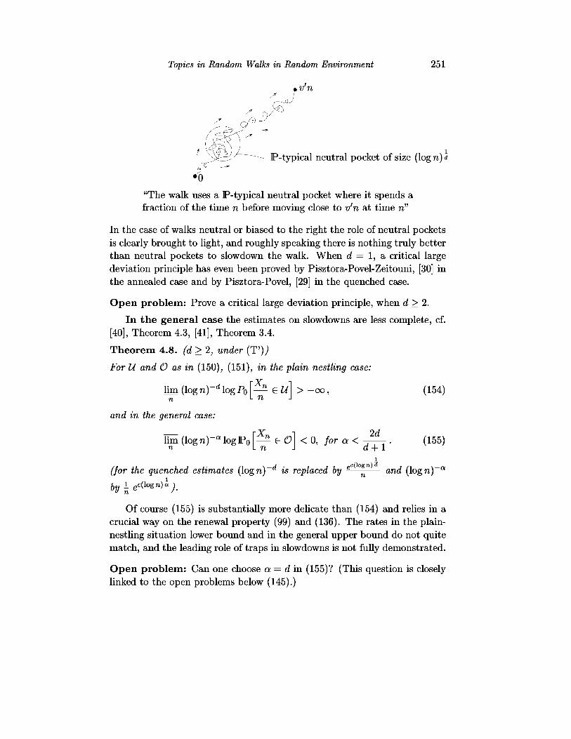
v'n

jyk^ls ~—~- P-typical neutral pocket of size (log n) a

"The walk uses a P-typical neutral pocket where it spends afraction of the time n before moving close to v'n at time n"

In the case of walks neutral or biased to the right the role of neutral pocketsis clearly brought to light, and roughly speaking there is nothing truly betterthan neutral pockets to slowdown the walk. When d — 1, a critical largedeviation principle has even been proved by Pisztora-Povel-Zeitouni, [30] inthe annealed case and by Pisztora-Povel, [29] in the quenched case.

Open problem: Prove a critical large deviation principle, when d > 2.

In the general case the estimates on slowdowns are less complete, cf.[40], Theorem 4.3, [41], Theorem 3.4.

Theorem 4.8. (d > 2, under (T))

For U and O as in (150), (151), in the plain nestling case:

Urn (logn)-d logPo \—€U] > -oo , (154)n L n J

and in the general case:

Ihn" (logn)"a logP0 f— G o] < 0, for a < -^- . (155)n I n J d + 1

i

(for the quenched estimates (logn) d is replaced by e° °^"— and (logn) a

by £ ec( l os")«;.

Of course (155) is substantially more delicate than (154) and relies in acrucial way on the renewal property (99) and (136). The rates in the plain-nestling situation lower bound and in the general upper bound do not quitematch, and the leading role of traps in slowdowns is not fully demonstrated.

Open problem: Can one choose a — dm. (155)? (This question is closelylinked to the open problems below (145).)

252 A.S. Sznitman

5 Small perturbations of the simple random walk

We now discuss some examples of walks satisfying condition (T"). In(117), we have already provided with the help of Kalikow's condition (112),some concrete examples where (T) and hence (T') hold. The class we nowdiscuss turns out to provide examples where (T') holds but Kalikow's con-dition breaks down.

We assume d > 3, and for e € (0,1) introduce

Se = {(p(e))|e|=i, with £ P(e) = 1 and \p(e) - ^ | < ^ for each e}

C V _ i in the notations of (60).K A A V ''id

(156)

The (2d)-vectors in Se should be viewed as "small perturbations" of thesimple random walk. Unlike [7], we investigate an anisotropic situation.

Theorem 5.1. (d > 3)

For 7] £ (0,1), there exists eo(d,r]) £ (0,1) such that for 0 < e < eo, whenthe single site distribution \i is supported on S£ and

A = E[d(0, ui) • ei] > 62"^, when d — 3 ,(157)

when d > 4,

then (T')|ei holds.

One interest of the above result is that it reads the ballistic nature ofthe walk directly from an expectation of the local drift with respect to thestatic measure P = //®z , and not from an expectation with respect to theso far unknown dynamic measure Q (cf. beginning of Lecture 1). As wewill later see the fact that the exponents of e which appear in (157) canexceed 2, plays an important role. It enables to construct examples of walksfor which (T')|ei holds but Kalikow's condition (K)\l is not fulfilled for any£ G 5 d - 1 . Let us also mention that (157) cannot be replaced by the weakerassumption A > 0, (for more on this see the remark following the sketch ofproof of Theorem 5.1, above (185)).

Sketch of proof, (for more details see [42]). This is an application of theeffective criterion (see (120)). One shows that for 0 < e < eo(d,rf) and A as


in (157)

with

(158)

(cf- ( "9) for t h e notations)

and S is the box in the figure below.

As mentioned before in checking (158) there is a problem of a possiblesmall denominator in ps corresponding to atypical exit distributions. Totake care of this difficulty we chop B in layers of thickness L ~ const e"1.Since /J, is concentrated on Se, the walk is pretty much comparable to asimple random walk if one only considers times up to the exit time from aslab of thickness 2L.

T L ~ const e~l

J A

• 0

i

Lo = NL,N = L3

L0 = \ (NLf

~ const e 4

One shows that for e < ei (d, 77)

< o—const Lo (159)

e-constLo. t e r m controlling exit of B

through dB n {z : sup |jzr • e,-| >i>2

254 A.S. Sznitman

with

p(O,u,)=sup { ^ 4 , xeB, x . e i = 0 } , (160)x ^p(X,UJ) i

where in the notations of (66):

q{x,«,) = 1 -p{x,«,) = PX,U,[T-L < TL\ • (161)

Define the slab U:U = {xt7Ld, | x . e i | < L } , (162)

then using the fact that Xn • e\ — XQ • e\ — Xô"1 d(Xk,w) • e\ is a PXjUJ-martingale and the stopping theorem we find

(163)

where

Tu-l

d(Xk,u) • ei Io (164)

gu(x,z,u})d(z,u) -eizeu

(gu stands for Green function of the walk killed outside U).Now since u(z, •) € Se for all z, L ~ const e"1 (const: small), one sees

with a comparison of Gu with Gv attached to the simple random walk that

p(0,w) < 3 4— we do not have a small denominator problem. (165)

One now wants to see that E[p(0,w)] < 1, and in essence this amounts toshowing that for

L>\UJ) = LrU\fl ' elj(.Uj , (^""]

E[D] dominates the fluctuations of Gu(d-ei)(x) one encounters when writing

(167)

Crucial controls: for a suitable c(d) > 0, when e < €2(^,77):

E[D] >2c\0L2, and (168)


2

P[\D(u) - E[D]| > u] < 2 exp ( - —}, for u > 0, (169)I. 2VD i

where VvD< e2~2, d — 3,

e, d > 5,

and Ao = el"1*, d = 3 , (cf. (157))= e3"^, d > 4 .

Then with these estimates one has

+ 3\{x € B, x • ei = 0}| P [L» - E[L>] < -cA0L2] .

<cons t (L 4 ) 3 ( d - 1 ) , . f— v ' <const exp - — c %j

° (170)

W \0L2 > const (d, r}) e^~v, d = 3,

const (d, rj) e1"77, d > 4,

and hence:A0L

2 > V^c • (171)

As a result for e < 63 (d, 77)

< l - f AOL,

and inserting this in (159), we find:

f / + e"C°nStL° <^ 2 1 /f1 — y / 1 — 2 o O

(172)and this is more than enough to prove (158).

Let us give some comments on the proof of (168), (169) which are thecrucial controls showing that the expectation of D dominates the relevantfluctuations of D around its mean. For instance for (168), we can write

E[£>] = E[(GtrA)(0)] + E[Gv(d • ei - A)(0)]. (173)

Now because Gu is close to G^, (see notations above (165)), it is no hardto see that:

(Gu\)(0) > c'(d) XL2 > c'(d) X0L2 (174)

256 A.S. Sznitman

so that the same holds for E[G[/(A)(0)]. One wants then to see that E[Gjj(d-e\ — A)(0)] is small compared to c'(d) XQL2. Observe that E[d(x,uj)-ei —A] =0, but \d(x, UJ) • e\ — A| can a-priori be of order ~ e > Ao (see below (169)),and to prove that E[Gjj(d • e\ — A)(0)] is small compared to c'{d) XQL2 oneneeds to use cancellations. One writes (see (118))

Gu(d• e i - A)(0) = TV] (175)

and introducing

Px,ui - Px,ux, where uJx(y, •) is w(y, •), for y x, and E[w(0, •)], for y - x ,(176)

one can single out the effect of ui(x: 0) in the denominator through:

TV]+

iei=1ii def

8(x,e)

Coming back to (175), using an expansion and the fact that:

— x Id v - < -

Tu]

(177)

8(x,e)Pl+e'"[Hx>Tu]

PA* <<K ~ K ~ 2

one finds:

Gu(d'ei-X)(0) = , where

(z, w) • ei - A)

^x,wl-nx > J-u\

(observe that using independence E[A] — 0)

{d(x, uj) • ei — A)B — —x(zjj Px,

\C\ < c(d)e3L2.

. Px

;, e) _P

x+eul[Hx

= l

(178)Note that e3L2 <C AoL2 for small e. However if one brutally bounds B, oneobtains \E[B]\ < conste2L2 and e2L2 ^> Ao-k2, which is a serious matter,since we plan to show that E[Gu(d • h - A)(0)] = E[A] + E[B] + E[C] issmall compared to c'(d)XoL2\


To overcome this difficulty, observe that

tf(z,e) = 0, (179)|e|=l

so we can introduce a counterterm in the last sum in B not depending on eand obtain:

B — — } =rJ—~ (d(x,uj) • ei — A)P [ H > J

E -J7 x Px+e,w[Hx > TJJ] — Px+eiUJ[Hx > TJJ]o(x,e) = ~

|e |=l Px,w[Hx > Tu]

and then one finds in a rather straightforward fashion

\E[B]\ < const e2 ^ gu(0,x,u) \gu(x + e,x,u) - gu(x + eux,u)\

with the notation of (164) for the Green function.Now the idea is that when x is in the bulk of U, i.e. far from dU, gu(x+

e, x, UJ) —gjj(x + ei,x, UJ) is close to the same expression where gjj is replacedby the Green function of the simple random walk, but because of the isotropyof the simple random walk, the corresponding expression vanishes. On theother hand when x is "close to dU", then gu(x + e,x,UJ) — gu(x + ei, x, UJ)need not be small but X^close to9*7 9U(0,X,CJ) <C L2 since the walk will notstay too long near the boundary of U where it can get killed. In fact oneshows:

|E[B]| < const e2 x (elogL + i ) L2 < A0L2 , (181)

and this is how the above "special cancellation of the e2L2 term" potentiallypresent in B enables to prove (168).

The bound (169) controlling the fluctuations of D is obtained by usingthe "martingale method" (see Proposition 3.2 of [42]), i.e. by consideringthe martingale

Hn = E[Gu(d • ei)(0)\Gn], with Qn =a(u(xu •), • • •,u>(xn, •)),

n > 0, {0, ft}, for n = 0 , (182)

(so Hn = Gv{d • ei)(0), Ho = E[Gtr(d- ei)(0)]),

with Xi,i > 1, an enumeration of U. By showing that

\Hn — Hn-i\ < 7n <— deterministic numbers, (183)

258 A.S. Sznitman

one finds with a slight variation on Azuma's inequality, cf. [1], that for u > 0,

2

n\Gu(d • ei)(0) - E[Gu(d • ei)(0)]| > u] < 2 exp { - ^ ^ } • (184)

"-1In spirit, to prove (169), one shows that

"7« < const ego,u(O,xn)"

where go,u(^,y) — (Gu^y)(x) is the Green function of the simple randomwalk killed outside U, (the actual control on j n are slightly weaker).

Note the heuristic bound on X!n>i Tn:

Y^ <?9o,u(°> x)2 ~ e2L ~ e « (A0L2)2, when d = 3,

e2 log L ~ elog - < (A0L2)2, when rf = 4,

e2 < (A0£2)2, when d > 5 .

This provides some rationale for the value of Ao, see (157) and (169). •

Remark: It is a natural question whether one can replace (157) with theweaker condition A > 0, and derive a similar conclusion. This is not the caseand some examples where E[d(0,w)] ^ 0, and the walk exhibits a diffusivebehavior can be found in the article [6]. •

Back to Kalikow's condition:

We now explain how the above result provides examples of walks for whichKalikow's condition does not hold for any I € Sd-1 but (T')|ei issatisfied.

In particular, unlike what is known to happen when d — 1, cf. [43],Kalikow's condition does not characterize ballistic behavior when d > 3.

To describe the example, we consider d > 3 , 0 < e < l , 0 pe2 , (186)

covP(w(0,ei),w(0,-ei)) < (1 - p) varp(w(0,ei)). (187)


One possible example of such a law corresponds to choosing an isotropicon .Si for which:

2

var^(p(ei)) > pe2, cov^(p(ei), p ( -e i ) ) < (1 - p) var?(p(ei)) (188)

and defining /i as the image of j2 under the map

p(e) -> p(e) + ^ e • ei, for |e| = 1 (189)

with A a number in (—^, ^ ) .

We now introduce

U+ = {y G Z d , y • ei > 0}, ?7_ = < 0} , (190)

and recall the definition of the auxiliary local drifts djj+(-) and djj_(-) in(111).

U- u+

Proposition 5.2. (under (185), (186), (187);

With A = E[d(0,w) • e\], provided:

K2

thendu+(0) = v+ei, dv_(0) = i/_ei, tui 0, ^_ < 0,

(191)

(192)

(and hence (K)\l fails for every £ G Sd 1).

Sketch of proof: Note that when R is a rotation preserving 7Ld, u G fi,

under Pa;,a;, (-R(^n))n>o is distributed as X n under

PR(x),Rw w i t n (Ru)(y,e) = ^ ( ^ " ^ y ) , .R" 1 ^) ) .(193)

260 A.S. Sznitman

Using (185) if R is a rotation preserving e\ and sending ej in —ei, for a giveni > 2, we see that for f7 = [/+ or U-, with the definitions (105), (111):

_

(because <ft/(0,0, Rw) — gjj(0,0,u}) and d(0, Rui) • ei — —d(0,uj) • ei) andhence

du(0) is colinear to ei, (recall here f7 is C/+ or U-). (194)

Moreover by an analogous calculation as in (175) - (178)

E[gu(0,0, u) d(0, u) • e{\ = au + pu + -ru, (195)

where with the notation (176), (177)

(where we have used (179) and Y,\e\=i ^(0>e) ^.wt-ffo <

l 7 l r | < 2 ( - ) (- <- because of (191)) .

We will now see that "/3j7 dominates". In contrast to the situation above(181), the boundary effects are now predominant. Indeed using indepen-dence:

|=l Po,o;[-ffo

Note that by (185) and (193),

E e '" ~ remains the same for all e with e • ei = 0. (196)


So using (179), we find:

Pu = -E\(6(0,ei) -S(0,-ei))(S(0,ei) + S(0,-ei))] E|

- £ *(0,e)e-ei=O

e=±ei

Note that because varp(w(0, ei)) = varp(w(O, —ei)) the first term vanishesand we find

(186)-(187)>/92e2

Pu = [varP(w(0, ei)) - covP(w(0, ei), w(0, -ei))]

0,o;[ >

Therefore specifying f7 = f7+ or f7_ we find

Pu+ > W2e2, Pu- < ~np2e2, (197)

and hence by (195) and (197)

^22 2 2 ^ y (198)

whereas

;)] < ^ e 2 - np2e2 + 2 ( ^ ) 3 (199)

and the claim (192) follows. •

Combining Theorem 5.1 and the above proposition, we see that for p, rj €(0,1), we can find H(d,r],p) € (0,1) such that when /J, concentrated on Se

satisfies (185), (186), (187) and

el"7* < A < ^ p2e2, when d = 3,(200)

e3"7? < A < y p2e2, when d > 4,

262 A.S. Sznitman

then (K)\e fails for every I € S"*"1, but (T')|ei satisfied (and the walk isballistic).

This concludes this brief account of some of the recent advances concern-ing random walks in random environment. Some of the ideas and paradigmsdiscussed in these notes are currently investigated for diffusions in randomenvironment, cf. [23],[34], and for dependent environments, cf. [9],[31],[45].Hopefully it will clear from reading these notes that although some issuesare better understood, much remains to be done.


References

[1] N. Alon, J. Spencer and P. Erdos, The probabilistic method, John Wiley& Sons, New York, 1992.

[2] V.V. Anshelevich, K.M. Khanin and Ya.G. Sinai, Symmetric randomwalks in random environments, Commun. Math. Phys., 85, 449-470(1982).

[3] D. Boivin, Weak convergence for reversible random walks in randomenvironment, Ann. Probab., 21(3), 1427-1440 (1993).

[4] E. Bolthausen and A.S. Sznitman, On the static and dynamicpoints of views for certain random walks in random environ-ment, to appear in Methods and Applications of Analysis,www.math.ethz.ch/~sznitman/preprint.shtml

[5] E. Bolthausen and A.S. Sznitman, Ten lectures on random media, DMVSeminar, Band 32, Birkhauser, Basel, 2002.

[6] E. Bolthausen and A.S. Sznitman and O. Zeitouni, Cut pointsand diffusive random walks in random environment, Preprint,www.math.ethz.ch/~sznitman/preprint.shtml

[7] J. Bricmont and A. Kupiainen, Random walks in asymmetric randomenvironments, Comm. Math. Phys., 142(2), 345-420 (1991).

[8] A.A. Chernov, Replication of a multicomponent chain, by the "lightningmechanism", Biophysics, 12, 336-341 (1962).

[9] F. Comets and O. Zeitouni, A law of large numbers for random walksin mixing environments, Preprint (2002).

[10] A. Dembo and Y. Peres and O. Zeitouni, Tail estimates for one-dimensional random walk in random environment, Comm. Math. Phys.,181, 667-683 (1996).

[11] A. Dembo and O. Zeitouni, Large deviations techniques and applica-tions, Springer, Berlin, 2nd edition, 1998.

[12] J.D. Deuschel and D.W. Stroock, Large deviations, Academic Press,Boston, 1989.

264 A.S. Sznitman

[13] R. Durrett, Probability: Theory and Examples, Wadsworth andBrooks/Cole, Pacific Grove , 1991.

[14] N. Enriquez and C. Sabot: A note on edge oriented reinforced randomwalks and RWRE, Preprint (2002).

[15] I. Fatt, The network model of porous media, III, Trans. Amer. Inst.Mining Metallurgical, and Petroleum Engineers, 207, 164-177 (1956).

[16] B.D. Hughes, Random walks and random environments, ClarendonPress, Oxford, Vol. 2, 1996.

[17] S.A. Kalikow, Generalized random walk in a random environment, Ann.Probab., 9, 753-768 (1981).

[18] H. Kesten, Sums of stationary sequences cannot grow slower than lin-early, Proc. Amer. Math. Soc, 49, 145-168 (1975).

[19] H. Kesten, The limit distribution of Sinai's random walk in randomenvironment Physica A, 138A, 299-309 (1986).

[20] H. Kesten and M.V. Kozlov and F. Spitzer, A limit law for randomwalk in a random environment, Compositio Mathematica, 30(2), 145-168 (1975).

[21] C. Kipnis and S.R.S. Varadhan, A central limit theorem for additivefunctionals of reversible Markov processes and applications to simpleexclusions, Comm. Math. Phys., 104, 1-19 (1986).

[22] S. Kirkpatrick, Classical transport in random media: scaling andeffective-medium theories, Phys. Rev. Letters, 27(25), 1722-1725 (1971).

[23] T. Komorowski and G. Krupa, On stationarity of Lagrangian observa-tions of passive tracer velocity in a compressible environment, Preprint,(2002).

[24] S.M. Kozlov, The method of averaging and walks in inhomogeneous en-vironments, Russian Math. Surveys, 40(2), 73-145 (1985).

[25] G.F. Lawler, Weak convergence of a random walk in a random environ-ment, Comm. Math. Phys., 87, 81-87 (1982).


[26] S.A. Molchanov, Lectures on random media, Ecole d'Ete de Probabilitiesde St. Flour XXII-1992, Editor P. Bernard, Vol. 1581, Lecture Notes inMath.. 242-411 (1994).

[27] S. Olla, Homogenization of diffusion processes in random fields, EcolePolytechnique, Palaiseau, 1994.

[28] G. Papanicolaou and S.R.S. Varadhan, Boundary value problems withrapidly oscillating random coefficients, in "Random Fields", J. Fritz, D.Szasz editors, Janyos Bolyai series, North-Holland. Amsterdam, 835-873, 1981.

[29] A. Pisztora and T. Povel, Large deviation principle for random walk ina quenched random environment in the low speed regime, Ann. Probab.,27(3), 1389-1413, (1999).

[30] A. Pisztora, T. Povel and O. Zeitouni, Precise large deviation estimatesfor one-dimensional random walk in random environment, Probab. The-ory Relat. Fields, 113, 191-219 (1999).

[31] F. Rassoul-Agha, The law of large numbers for random walks in a mix-ing environment, Preprint, (2002).

[32] P. Revesz, Random walk in random and non-random environments,World Scientific, Singapore, 1990.

[33] W. Rudin, Functional analysis, Tata Me Graw-Hill, New Delhi, 1974.

[34] L. Shen, On ballistic diffusions in random environment, Preprint, May2002.

[35] Ya.G. Sinai, The limiting behavior of a one-dimensional random walkin a random environment, Theory Prob. Appl., 27(2), 247-258 (1982).

[36] F. Solomon, Random walk in a random environment, Ann. Probab., 3,1-31 (1975).

[37] A.S. Sznitman, Brownian motion, obstacles and random media,Springer, Berlin, 1998.

[38] A.S. Sznitman, Slowdown and neutral pockets for a random walk in ran-dom environment, Probab. Theory Relat. Fields 115, 287-323 (1999).

266 A.S. Sznitman

[39] A.S. Sznitman, Slowdown estimates and central limit theorem for ran-dom walks in random environment, J. Eur. Math. Soc, 2, 93-143 (1999).

[40] A.S. Sznitman, On a class of transient random walks in random envi-ronment, Ann. Probab., 29(2), 723-764 (2001).

[41] A.S. Sznitman, An effective criterion for ballistic behavior of randomwalks in random environment, Probab. Theory Relat. Fields, 122(4),509-544 (2002).

[42] A.S. Sznitman, On new examples of ballistic random walks in randomenvironment,to appear in Ann. Probab., www.math.ethz.ch/~sznitman/preprint.shtml.

[43] A.S. Sznitman and M.P.W. Zerner, A law of large numbers for randomwalks in random environment, Ann. Probab., 27(4), 1851-1869 (1999).

[44] D.E. Temkin, One-dimensional random walks in a two-componentchain, Soviet Math. Dokl., 13(5), 1172-1176 (1972).

[45] O. Zeitouni, Notes of Saint Flour lectures 2001, Preprint,www-ee.technion.ac.il/~zeitouni/ps/notesl.ps.

[46] M.P.W. Zerner, Lyapunov exponents and quenched large deviation formultidimensional random walk in random environment, Ann. Probab.,26, 1446-1476 (1998).

[47] M.P.W. Zerner, Velocity and Lyapounov exponents of some randomwalks in random environment, Ann. Inst. Henri Poincare, Probabiliteset Statistiques, 36(6), 737-748 (2000).

[48] M.P.W. Zerner and F. Merkl, A zero-one law for planar random walksin random environment, Ann. Probab., 29(4), 1716-1732, (2001).

Topics in Random Walks in Random Environment - OSTI.GOV

Documents