Random trees and vertex splitting Thordur Jonsson, University of Iceland September 2009 Statistical physics, combinatorics and probability: from discrete to continuous models Institut Henri Poincare 1 / 57

Welcome message from author
This document is posted to help you gain knowledge. Please leave a comment to let me know what you think about it! Share it to your friends and learn new things together.
Transcript

Random trees and vertex splitting
Thordur Jonsson, University of Iceland
September 2009
Statistical physics, combinatorics and probability: from discrete tocontinuous models
Institut Henri Poincare
1 / 57

Outline
I Introduction and background
I Definition of the vertex splitting model
I Vertex degree distribution
I Correlations
I Structure functions and the Hausdorff dimension
I Open problems
2 / 57

Random graphs: two main approaches
1. Equilibrium statistical mechanics
T = Set of graphs, � a probability measure on T
�(T ) = Z�1e��E(T )
2. Growing trees Tn 7! Tn+1, time discrete
Stochastic growth rules induce a probability measure on Tt,the trees that can arise in t steps
I Sometimes (1) is more natural
I Sometimes (2) is more natural
I Sometimes (1) and (2) are known to be equivalent
3 / 57

Galton-Watson trees
I pn = probability of having n descendents,
Xn
pn = 1; m =Xn
npn
I m < 1 subcritical, m > 1 supercritical, m = 1 critical
I n generations at time t = n� 1 if no extinction
I Well understood
4 / 57

Preferential attachment trees
I In each timestep one new edge is attached to a preexisting tree
I Probability of attaching to a vertex v of degree k
Pv =wkP
k nkww; wk � 0;
nk = the number of vertices of degree k.
I Growth rule induces a probability measure on Tt.
5 / 57

Local trees
I Weight factor of a tree T
W (T ) =Yi2T
w�(i)
�(i) = degree of the vertex i
I Partition functions
ZN =X
T :jT j=N
W (T ); Z =XN
�NZN ; j�j < �0
I Generating function g(z) =P
nwnzn�1, radius of
convergence �
I Main equation
&%'$ &%
'$
&%'$
&%'$
u uu
uu
uu
= + � � �+ +
w2 w3
6 / 57

Generic trees
&%'$ &%
'$
&%'$
&%'$
u uu
uu
uu
= + � � �+ +
w2 w3
I Algebraically
Z(�) = �g(Z(�)) = �1Xi=0
wi+1Zi(�)
I Define Z0 = lim�!�0 Z(�)
I If Z0 < � then we say that the trees are generic.
I Z(�)� Z0 �p�0 � �
7 / 57

I Define�(T ) = Z�1
0 �jT j0
Yi2T
w�(i)
Probability measure
I This measure is the same as the one obtained from aGalton-Watson process with
pn = �0wn+1Zn�10
8 / 57

I Define�(T ) = Z�1
0 �jT j0
Yi2T
w�(i)
Probability measure
I This measure is the same as the one obtained from aGalton-Watson process with
pn = �0wn+1Zn�10
8 / 57

Another equivalence
I Preferential attachment trees � Causal trees
I Weight proportional to the number of causal labelings
0
1
2
9
53
4
8
10 6
7
I More branchings, more ways to grow
9 / 57

Properties of generic trees
I Let VT (R)=volume of a ball of radius R centered on the root
hVT (R)i � RdH ; R!1 de�nes dH
I Let pT (t) = probability that a random walker is back at theroot after t steps on T
hpT (t)i � t�ds=2; t!1 de�nes ds
10 / 57

Properties of generic trees
I Let VT (R)=volume of a ball of radius R centered on the root
hVT (R)i � RdH ; R!1 de�nes dH
I Let pT (t) = probability that a random walker is back at theroot after t steps on T
hpT (t)i � t�ds=2; t!1 de�nes ds
10 / 57

Properties of generic trees
I Let VT (R)=volume of a ball of radius R centered on the root
hVT (R)i � RdH ; R!1 de�nes dH
I Let pT (t) = probability that a random walker is back at theroot after t steps on T
hpT (t)i � t�ds=2; t!1 de�nes ds
10 / 57

Properties of generic trees
I Let VT (R)=volume of a ball of radius R centered on the root
hVT (R)i � RdH ; R!1 de�nes dH
I Let pT (t) = probability that a random walker is back at theroot after t steps on T
hpT (t)i � t�ds=2; t!1 de�nes ds
10 / 57

I Averages taken w.r.t. a measure on infinite trees
�N = Z�1N
Yi2T
w�(i)
�N ! �1 as N !1
I Properties:
(i) dH = 2(ii) ds = 4=3(iii) There is a unique infinite simple path whose outgrowths are
critical GW-trees
11 / 57

I Averages taken w.r.t. a measure on infinite trees
�N = Z�1N
Yi2T
w�(i)
�N ! �1 as N !1
I Properties:
(i) dH = 2(ii) ds = 4=3(iii) There is a unique infinite simple path whose outgrowths are
critical GW-trees
11 / 57

Preferential attachment trees
I In general many infinite simple paths
I dH =1 in many cases (all cases?)
I Can calculate vertex degree distribution - and fluctuations.Independent of the initial tree.
I Broad distribution of sizes of subtrees, depends on the initialtree
12 / 57

The vertex splitting model
F. David, M. Dukes, S. Stefansson and T.J.: J. Stat. Mech.(2009) P04009
I A model of randomly growing rooted, planar trees
vv
V
V’V’
V
v’
I Degree of vertices is bounded by an integer d (we also discussthe case d =1)
I Nonnegative splitting weights w1; w2; : : : ; wd
I nj(T ) = the number of vertices of degree j in a tree Tpj = Probability of choosing a vertex v 2 T of degree j
pj =wjP
iwini(T )13 / 57

Splitting rulesI The parameters of the model are2
666666664
0 w1;2 w1;3 � � � w1;d�1 w1;d
w2;1 w2;2 w2;3 � � � w2;d�1 w2;d
w3;1 w3;2 w3;3 � � � w3;d�1 0
w4;1 w4;2 w4;3 0 0...
......
......
...wd;1 wd;2 0 � � � 0 0
3777777775
a symmetric matrix of non–negative partitioning weightsI Split a vertex of degree i into vertices of degree k andi+ 2� k with probability wk;i+2�k=wi – all such splittingsequally probable
I The splitting weights w1; w2; : : : ; wd are related to thepartitioning weights by
wi =i
2
i+1Xj=1
wj;i+2�j :
14 / 57

A tree
15 / 57

Vertex splitting rules
w3
16 / 57

Vertex splitting rules
17 / 57

Vertex splitting rules
w2;3
18 / 57

Vertex splitting rules
19 / 57

Vertex splitting rules
w2;3
20 / 57

Vertex splitting rules
21 / 57

Vertex splitting rules
w1;4 = w4;1
22 / 57

Vertex splitting rules
23 / 57
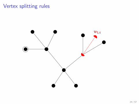
Vertex splitting rules
w1;4
24 / 57

Vertex splitting rules
25 / 57

Vertex splitting rules
w1;4
26 / 57

Relation to other models
I Ergodic moves in Monte Carlo simulations of triangulations in2d-quantum gravity
vvv’
I A tree growth process which arises in the study of RNAsecondary structures F. David, C. Hagendorf, K. J. Wiese
I When wi;j = 0 unless j = 1 or i = 1 it reduces to thepreferential attachment model
I For d = 3, in a certain limit, it reduces to Ford’s alpha modelfor phylogenetic trees
27 / 57

Main results
I Distribution of vertex degrees in a large tree
I Correlations between the degrees of vertices
I ”Shape” of trees – Hausdorff dimension
If we consider linear splitting weights
wi = ai+ b:
the analysis simplifies due to the Euler relation for trees
dXi=1
ni(T ) = jT j;dX
i=1
ini(T ) = 2(jT j � 1):
The normalization factorP
iwini(T ) depends only on the size ofthe tree T .
28 / 57

Recurrence for generating functions
Let pt(n1; : : : ; nd) be the probability that the tree T at time t has(n1(T ); : : : ; nd(T )) = (n1; : : : ; nd) .The probability generating function
Ht(x) =X
n1+���nd=t
pt(n1; : : : ; nd)xn11 � � �xndd
satisfies the recurrence
Ht+1(x) =X
n1+���+nd=t
pt(n1; : : : ; nd)Pdi=1 niwi
c(x) � r(xn11 � � �xndd );
where c(x) = (c1(x); c2(x); : : : ; cd(x)) with
ci(x) =i
2
i+1Xj=1
wj;i+2�jxjxi+2�j and r =�@=@x1; : : : ; @=@xd
�:
29 / 57

Vertex degree distribution
I Begin with a tree T0 at time 0
I At time t > 0 we have a tree Tt with ni(Tt) vertices of degreei
I Let �nt;i denote the average of ni(T ) over all trees that canarise at time t, i.e.
10 F. DAVID, W.M.B. DUKES, T. JONSSON, S.O. STEFANSSON.
The partial derivative !/!xi in ! takes care of removing a vertex of degreei and provides the factor ni. In ci(x), the factors xjxi+2!j add two verticesof degree j and i + 2" j respectively and the appropriate weights are given.Now sum over all possible partitionings in (iii), the dot product of c(x) and! accounts for the sum over all vertex degrees, and finally sum over allvertex degree configurations in the initial tree to obtain (2.10). !
For linear weights (2.5), equation (2.10) reduces to
Ht+1(x) =1
W(t)c(x) ·!Ht(x). (2.13)
The remainder of this subsection concerns linear weights only. We have
nt,k =!
n1+...+nd=t
pt(n1, ..., nd)nk = !kHt(x)|x=1, (2.14)
where 1 = (1, 1, . . . , 1). To get a recursion equation for nt,k, di!erentiateboth sides of (2.13) with respect to xk and set x = 1 to find
nt+1,k =1
W(t)
"d!
i=k!1
iwk,i+2!knt,i +d!
i=1
wi!i!kHt(x)|x=1
#.
(2.15)
Since the weights are linear we can use the constraints in (2.7) to rewritethe last term in (2.15) as
d!
i=1
wi!i!kHt(x)|x=1 = ("wk +W(t))nt,k. (2.16)
Inserting this into (2.15) we see that the equations close
nt+1,k =1
W(t)
""wknt,k +
d!
i=k!1
iwk,i+2!knt,i
#+ nt,k. (2.17)
We can also write the recursion in terms "t,k and find
"t+1,k =t
W(t)
""wk"t,k +
d!
i=k!1
iwk,i+2!k"t,i
#+ t("t,k " "t+1,k). (2.18)
The above equation can be put in the matrix form
!t+1 = At !t (2.19)
where
!t = ("t,1, "t,2, . . . , "t,d)T , At =
t
t + 1
"I +
1W(t)
B
#,
(2.20)
I Define
�t;i =�nt;it
and we will use the notation
�(t) = (�t;1; : : : ; �t;d)
30 / 57

I The recurrence for Ht gives rise to a recurrence for �(t).
10 F. DAVID, W.M.B. DUKES, T. JONSSON, S.O. STEFANSSON.
The partial derivative !/!xi in ! takes care of removing a vertex of degreei and provides the factor ni. In ci(x), the factors xjxi+2!j add two verticesof degree j and i + 2" j respectively and the appropriate weights are given.Now sum over all possible partitionings in (iii), the dot product of c(x) and! accounts for the sum over all vertex degrees, and finally sum over allvertex degree configurations in the initial tree to obtain (2.10). !
For linear weights (2.5), equation (2.10) reduces to
Ht+1(x) =1
W(t)c(x) ·!Ht(x). (2.13)
The remainder of this subsection concerns linear weights only. We have
nt,k =!
n1+...+nd=t
pt(n1, ..., nd)nk = !kHt(x)|x=1, (2.14)
where 1 = (1, 1, . . . , 1). To get a recursion equation for nt,k, di!erentiateboth sides of (2.13) with respect to xk and set x = 1 to find
nt+1,k =1
W(t)
"d!
i=k!1
iwk,i+2!knt,i +d!
i=1
wi!i!kHt(x)|x=1
#.
(2.15)
Since the weights are linear we can use the constraints in (2.7) to rewritethe last term in (2.15) as
d!
i=1
wi!i!kHt(x)|x=1 = ("wk +W(t))nt,k. (2.16)
Inserting this into (2.15) we see that the equations close
nt+1,k =1
W(t)
""wknt,k +
d!
i=k!1
iwk,i+2!knt,i
#+ nt,k. (2.17)
We can also write the recursion in terms "t,k and find
"t+1,k =t
W(t)
""wk"t,k +
d!
i=k!1
iwk,i+2!k"t,i
#+ t("t,k " "t+1,k). (2.18)
The above equation can be put in the matrix form
!t+1 = At !t (2.19)
where
!t = ("t,1, "t,2, . . . , "t,d)T , At =
t
t + 1
"I +
1W(t)
B
#,
(2.20)
=)
10 F. DAVID, W.M.B. DUKES, T. JONSSON, S.O. STEFANSSON.
The partial derivative !/!xi in ! takes care of removing a vertex of degreei and provides the factor ni. In ci(x), the factors xjxi+2!j add two verticesof degree j and i + 2" j respectively and the appropriate weights are given.Now sum over all possible partitionings in (iii), the dot product of c(x) and! accounts for the sum over all vertex degrees, and finally sum over allvertex degree configurations in the initial tree to obtain (2.10). !
For linear weights (2.5), equation (2.10) reduces to
Ht+1(x) =1
W(t)c(x) ·!Ht(x). (2.13)
The remainder of this subsection concerns linear weights only. We have
nt,k =!
n1+...+nd=t
pt(n1, ..., nd)nk = !kHt(x)|x=1, (2.14)
where 1 = (1, 1, . . . , 1). To get a recursion equation for nt,k, di!erentiateboth sides of (2.13) with respect to xk and set x = 1 to find
nt+1,k =1
W(t)
"d!
i=k!1
iwk,i+2!knt,i +d!
i=1
wi!i!kHt(x)|x=1
#.
(2.15)
Since the weights are linear we can use the constraints in (2.7) to rewritethe last term in (2.15) as
d!
i=1
wi!i!kHt(x)|x=1 = ("wk +W(t))nt,k. (2.16)
Inserting this into (2.15) we see that the equations close
nt+1,k =1
W(t)
""wknt,k +
d!
i=k!1
iwk,i+2!knt,i
#+ nt,k. (2.17)
We can also write the recursion in terms "t,k and find
"t+1,k =t
W(t)
""wk"t,k +
d!
i=k!1
iwk,i+2!k"t,i
#+ t("t,k " "t+1,k). (2.18)
The above equation can be put in the matrix form
!t+1 = At !t (2.19)
where
!t = ("t,1, "t,2, . . . , "t,d)T , At =
t
t + 1
"I +
1W(t)
B
#,
(2.20)31 / 57

I Under mild conditions on the wi;j the limits
limt!1
�t;i = �i
exist and are the unique positive solution to the linearequations
�k = �wk
w2�k +
dXi=k�1
iwk;i+2�k
w2�i:
I These values are independent of the initial tree.
I The proof uses the Perron–Frobenius theorem for ”positive”matrices.
32 / 57

I Under mild conditions on the wi;j the limits
limt!1
�t;i = �i
exist and are the unique positive solution to the linearequations
�k = �wk
w2�k +
dXi=k�1
iwk;i+2�k
w2�i:
I These values are independent of the initial tree.
I The proof uses the Perron–Frobenius theorem for ”positive”matrices.
32 / 57

I Under mild conditions on the wi;j the limits
limt!1
�t;i = �i
exist and are the unique positive solution to the linearequations
�k = �wk
w2�k +
dXi=k�1
iwk;i+2�k
w2�i:
I These values are independent of the initial tree.
I The proof uses the Perron–Frobenius theorem for ”positive”matrices.
32 / 57

Perron-Frobenius
Theorem. Let A be a matrix with nonnegative matrix elementssuch that all the matrix elements of Ap are positive (A primitive)for some integer p. Then the eigenvalue of A with the largestabsolute value is positive and simple. The correspondingeigenvector can be taken to have positive entries.
Iterating the recurrence equation for �(t) we find
�(t) =1
t
t�1Yi=1
�1 +
1
(2a+ b)i� 2aB
��0
where B is a matrix with nonnegative entries except on thediagonal. If B is primitive and diagonalizable, then �(t) convergesto the normalized Perron-Frobenius eigenvector of B.
33 / 57

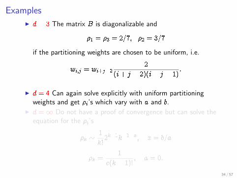
Examples
I d = 3 The matrix B is diagonalizable and
�1 = �3 = 2=7; �2 = 3=7
if the partitioning weights are chosen to be uniform, i.e.
wi;j = wi+j�22
(i+ j � 2)(i+ j � 1):
I d = 4 Can again solve explicitly with uniform partitioningweights and get �i’s which vary with a and b.
I d =1 Do not have a proof of convergence but can solve theequation for the �i’s
�k � 1
k!2k�1k�1�x; x = b=a
�k =1
e(k � 1)!; a = 0:
34 / 57

General splitting weightsI Use mean field theory for the normalization factorP
i ni(T )wi ! tP
i �iwi.Equation for a steady state vertex distribution
�k = �wk
w�k +
dXi=k�1
iwk;i+2�k
w�i;
subject to the constraints
�1 + : : :+ �d = 1; w1�1 + : : :+ wd�d = w:
I There is a unique positive solution by the Perron-Frobeniustheorem.
I For d = 3 and uniform partitioning weights we find
�3 =7��p� (�+ 24� + 24)
6(2�� � � 1)
where � = w2=w1 and � = w3=w1.
35 / 57

Comparison with simulations
16 F. DAVID, W.M.B. DUKES, T. JONSSON, S.O. STEFANSSON.
The solution to the mean field equation for the d = 3 model and uniformpartitioning weights is
!3 =7" !
!" (" + 24# + 24)
6(2" ! # ! 1)(2.45)
where " =w2
w1and # =
w3
w1. Note that from the constraints we have !1 = !3
and !2 = 1 ! 2!3. This solution (and solutions in general) only dependson the ratio of the weights. In Figure 4 we compare the above solution tosimulations.
0
0.1
0.2
0.3
0.4
0.5
0 20 40 60 80
! = 10000
! = 1000
! = 100
! = 10
! = 0
"
#3
Figure 4. The value of !3 as given in (2.45) compared toresults from simulations. Each point is calculated from 20trees on 10000 vertices.
2.6. The dmax = " model with linear weights. In this subsection wedrop the assumption that there is an upper bound on the vertex degreesbut we still assume that all vertex degrees are finite. If we assume thatequation (2.35) holds for d =", then it is possible to find an exact solutionin the case of linear splitting weights, wi = ai + b, and uniform partitioningweights. Equation (2.35) becomes
!k = !wk
w2!k +
!"
i=k"1
2i + 1
wi
w2!i. (2.46)
Subtracting from this the same equation for !k+1 we find
!k
#1 +
wk
w2
$! !k+1
#1 +
wk+1
w2
$=
2k
wk"1
w2!k"1. (2.47)
A comparison of the theoretical prediction with simulations in thecase d=3 and uniform partitioning weights.
� =w2
w1; � =
w3
w1
36 / 57

Correlations
In a typical infinite tree, what is the proportion of edges whoseendpoints have degrees j and k ?
Let nj;k = number of such edges in a finite tree of size t, wherethe vertex of degree j is closer to the root
Let �j;k = limt!1nj;kt
. Then (for linear splitting weights)
�jk = �wj + wk
w2�jk + (j � 1)
wj;k
w2�j+k�2
+(j � 1)dX
i=j�1
wj;i+2�j
w2�ik + (k � 1)
dXi=k�1
wk;i+2�k
w2�ji:
assuming the existence of the limit.
37 / 57

Explicit solutions
Can solve in simple cases and find nontrivial correlationsTake d = 3, linear splitting weights and uniform partitioningweights. Then �1 = �3 = 2=7 and �2 = 3=7. Let y = w3=w2.Then the solutions to the correlation equation are
�21 =4(3� y)
7(11� 2y); �31 =
10
7(11� 2y);
�22 =4y2 � 12y + 105
7(2y + 7)(11� 2y); �32 =
2(�8y2 + 18y + 63)
7(2y + 7)(11� 2y);
�23 =2(�4y2 + 20y + 21)
7(2y + 7)(11� 2y); �33 =
8(3y � 14)
7(2y + 7)(2y � 11):
38 / 57

Sum rules
The following sum rules hold:
�21 + �31 = �1 = 2=7�22 + �32 = �2 = 3=7�23 + �33 = �3 = 2=7;
�21 + �22 + �23 = �2 = 3=7�31 + �32 + �33 = 2�3 = 4=7:
These relations show that there are only two independent linkdensities, e.g. �21 and �22.
39 / 57

Comparison with simulations
RANDOM TREE GROWTH BY VERTEX SPLITTING 33
!21 =4(3! y)
7(11! 2y), !31 =
107(11! 2y)
,
!22 =4y2 ! 12y + 105
7(2y + 7)(11! 2y), !32 =
2(!8y2 + 18y + 63)7(2y + 7)(11! 2y)
,
!23 =2(!4y2 + 20y + 21)7(2y + 7)(11! 2y)
, !33 =8(3y ! 14)
7(2y + 7)(2y ! 11).
(5.2)
Note that the following sum rules hold for the solutions
!21 + !31 = !1 = 2/7!22 + !32 = !2 = 3/7!23 + !33 = !3 = 2/7,
!21 + !22 + !23 = !2 = 3/7!31 + !32 + !33 = 2!3 = 4/7.
(5.3)
These relations show that there are only two independent link densities. Weplot !21 and !22 in Figure ?? and compare to simulations.
0.05
0.1
0.15
0.2
0.25
0 0.5 1 1.5 2
y
!21!22
Figure 15. Two independent solutions given in (??) plot-ted against y = w3/w2 and compared to simulations. Thetwo leftmost datapoints on each line come from simulationsof 50 trees on 50000 vertices. The other datapoints comefrom simulations of 50 trees on 10000 vertices.
We can compare the above results to the case when no correlations arepresent. Denote the uncorrelated densities by !ij . Then we simply have
!ij =!i!j
1! !1.
40 / 57

Nonlinear splitting weights
Taking d = 3 and general nonlinear splitting weights
�21 =1
3
(3 + �) (7�� )
(2�� � � 1) (3�+ 2� + + 6)
where � = w2=w1, � = w3=w1 and =p� (�+ 24� + 24).36 F. DAVID, W.M.B. DUKES, T. JONSSON, S.O. STEFANSSON.
0
0.02
0.04
0.06
0.08
0.1
0.12
0 20 40 60 80 100
!2
1
"
# = 2
# = 10
# = 60
# = 100
Figure 16. The solution (5.4) for the density !21 plottedas a function of " for a few values of #. Each datapoint iscalculated from simulations of 100 trees on 10000 vertices.
0
0.1
0.2
0.3
0.4
0.5
0.6
0.7
0 20 40 60 80 100
!2
2
"
# = 100
# = 2
# = 60
# = 10
Figure 17. The solution (5.5) for the density !22 plottedas a function of " for a few values of #. Each datapoint iscalculated from simulations of 100 trees on 10000 vertices.
41 / 57

Comparison with simulations
36 F. DAVID, W.M.B. DUKES, T. JONSSON, S.O. STEFANSSON.
0
0.02
0.04
0.06
0.08
0.1
0.12
0 20 40 60 80 100
!2
1
"
# = 2
# = 10
# = 60
# = 100
Figure 16. The solution (5.4) for the density !21 plottedas a function of " for a few values of #. Each datapoint iscalculated from simulations of 100 trees on 10000 vertices.
0
0.1
0.2
0.3
0.4
0.5
0.6
0.7
0 20 40 60 80 100
!2
2
"
# = 100
# = 2
# = 60
# = 10
Figure 17. The solution (5.5) for the density !22 plottedas a function of " for a few values of #. Each datapoint iscalculated from simulations of 100 trees on 10000 vertices.
RANDOM TREE GROWTH BY VERTEX SPLITTING 35
We can compare the above results to the case when no correlations arepresent. Denote the uncorrelated densities by !ij. Then we simply have
!ij =!i!j
1! !1.
The denominator comes from the fact that the vertex closer to the root isof degree one with probability zero. Inserting the values from (5.3) into thisequation gives
!21 = 6/35, !31 = 4/35!22 = 9/35, !32 = 6/35!23 = 6/35, !33 = 4/35
showing that in general !ij "= !ij and so correlations are present betweendegrees of vertices.
5.3. Results for non-linear weights. We can generalize equation (5.1)to a mean field equation, valid for arbitrary weights, by replacing w2, whereit appears in a denominator, with w as we did with the equation for vertexdegree densities in Section 2. For d = 3 and uniform partitioning weightsthe two independent densities !21 and !22 are given by
!21 =13
(3 + ") (7#! $)(2#! " ! 1) (3# + 2" + $ + 6)
(5.4)
!22 = 16
3
“284 !2"
4# ! 177 !5"# + 3564 !3 + 18 !6# + 161! "5# ! 873 # + 11979 !2"3
!2259 !5 ! 39 !6" ! 207 !5# + 6516!2"4 ! 5205 !5" ! 1419 !4"# + 996 !"5
!5994 !4 ! 892 !4"2# + 1543 !2"5 ! 18 !7 ! 668 !3"4 + 324 !2# + 909 !"3#
!2600 !5"2 ! 975 !3"3 + 222 !"6 ! 1533 !3"2# + 10206 !2"2 ! 11799 !4"
!5300 !4"3 ! 1521 !3"# + 1899 !2"2# + 1059!2 "3# + 1269 !3"2 + 3240!2 "
+756 !"3 + 4860 !3" + 6 "6# ! 11703 !4"2 + 1728!2 "# ! 162 !3# + 486! "2#
+18 "4# + 1530 !"4 + 624! "4# ! 772 !3"3# ! 9 !6 + 24 "5#”.“
(3 ! + 2 " + # + 6)
"`11 !2 + 25 !" + 5 !# + 3 "# + 12 ! + 4 "2
´(!! + #) (1! 2 ! + ") (7 ! + 2 " + #)2
”
(5.5)
where # =w2
w1, " =
w3
w1and $ =
!# (# + 24" + 24). These solutions
are compared to simulations in Figures 16 and 17. The other densities areobtained by using the sum rules (5.3).
42 / 57

Subtree probabilities
I Label vertices in the tree by their time of creation
I Use linear weights
I Derive expressions for the probabilistic structure of the tree asseen from the vertex created at a given time
I Average over the creation time
I Introduce a scaling assumption
I Extract the Hausdorff dimension
I Get results which agree with simulations
43 / 57

I Begin with a tree consisting of a single vertex at time t = 0
I In a tree of size ` let pR(`; s) be the probability that thevertex created at time s � ` is the root
I We find
pR(`; s) =1
W (`� 1) + w1W (`� 1)pR(`� 1; s); s < `
pR(`; `) =1
W (`� 1) + w1
`�1Xs=0
w1pR(`� 1; s); s = `
W (`) = (2a+ b)`� a is a normalization factor.
44 / 57

18 F. DAVID, W.M.B. DUKES, T. JONSSON, S.O. STEFANSSON.
Figure 6. Diagrams representing equations (??) and (??).
If v is a vertex of order k in a tree T , then there is a unique link !1 incidenton v leading towards the root (unless v is the root). Let !2, . . . , !k be theother links incident on v. The largest subtree of T which contains the rootand !1 but none of the links !i with i ! 2 will be called the left subtree (withrespect to v). The maximal subtrees which contain one !j with j "= 1 andno other link !i will be called the right subtrees (with respect to v). If k = 1then there are of course no right subtrees and if v is the root then we viewthe left subtree as being empty. Let pk(!1, . . . , !k; s) denote the probabilitythat the vertex created at time s has a left subtree on !1 edges and rightsubtrees on !2, . . . , !k edges, where !1 + . . . + !k = !. By the nature of thesplitting operation, pk(!1, !2, . . . , !k; s) is symmetric under permutations of(!2, . . . , !k). We will sometimes refer to the vertex created at time s as thes-vertex.
By the definition of the relabeling when we split we have
p1(!; !) = 0, (3.4)
because the vertex closer to the root gets a new label and therefore no leafexcept the root can have the maximal label. In the case s < ! we find therecursion
p1(!; s) =1
W (!# 1) + w1
!W (!# 1)p1(!# 1; s)
+d!1"
i=1
iwi+1,1
"
!!1+...+!!
i=!!1
pi(!"1, . . . , !"i; s) + "!1w1
#.
(3.5)
The first term in the square bracket corresponds to the case when we donot split the vertex with label s. The second term corresponds to splittingthe s-vertex which can have any order up to d # 1. Finally the last termcorresponds to the special case when we have ! = 1 so the s-vertex is theroot of the trivial tree, see Fig. ??.
Let pk(`1; `2; : : : ; `k; s) be the probability that the vertex v createdat time s has degree k, the root subtree has `1 links and the othersubtrees incident on v have size `2; : : : ; `k. Denote the sum of the`i’s by `. Then for k = 1 and s < `RANDOM TREE GROWTH BY VERTEX SPLITTING 19
Figure 7. A diagram representing equation (??).
For a general k ! 2 and s < ! the recursion can be written
pk(!1, . . . , !k; s) =1
W (!" 1) + w1#
!"k2"!11w1pR(!" 1; s) +
k"
i=1
W (!i " 1)pk(!1, . . . , !i " 1, . . . , !k; s) (3.6)
+d"
i=k
(i + 1" k) wk,i!k+2
"
!!1+...+!!i+1"k=!1!1
pi(!"1, . . . , !"i+1!k, !2, . . . , !k; s)
#,
see Fig.??. The first term corresponds to the case when the s-vertex is theroot before the splitting in which case we have !1 = 1 and k = 2. Thesecond term corresponds to the case when we split a vertex di!erent fromthe s-vertex and the last term arises when we split the s-vertex in the stepfrom time !" 1 to time !. Finally we have
pk(!1, . . . , !k; !) =1
W (!" 1) + w1# (3.7)
!!1"
s=0
k"
j=2
d!1"
i=k!1
"
!!1+...+!!i+1"k
=!j"1
wk,i!k+2pi(!1, . . . , !j!1, !"1, . . . , !
"i+1!k, !j+1, . . . , !k; s),
where !1 + . . . + !k = !, see Fig.??. Here s is the label of the vertex thatis split in the step from time ! " 1 to time ! and we sum over all possibledegrees of the s-vertex and all ways of splitting it.
We define the following mean probabilities by averaging over the vertexlabels in (??–??)
pR(!) =1
! + 1
!"
s=0
pR(!; s) (3.8)
45 / 57

and for k > 1 and s < `RANDOM TREE GROWTH BY VERTEX SPLITTING 21
Figure 8. A diagram representing equation (3.6).
and
pk(!1, . . . , !k) =1
! + 1
!!
s=0
pk(!1, . . . , !k; s), (3.9)
where !1 + . . . + !k = ! From (3.8) we get a recursion for the mean proba-bilities, going from time ! to ! + 1
pR(! + 1) =! + 1! + 2
pR(!). (3.10)
For k = 1 we obtain from (3.4), (3.5) and (3.9)
p1(! + 1) (3.11)
=! + 1! + 2
1W (!) + w1
"W (!)p1(!) +
d!1!
i=1
iwi+1,1
!
!!1+...+!!i
=!
pi(!"1, ..., !"i) + 2"!0w1
#.
46 / 57

Finally k > 1 and s = `22 F. DAVID, W.M.B. DUKES, T. JONSSON, S.O. STEFANSSON.
Figure 9. A diagram representing equation (3.7).
Finally, the general case for k ! 2 is
pk(!1, . . . , !k)
=! + 1! + 2
1W (!) + w1
!"k2"!11w1pR(!) +
k"
i=1
W (!i " 1)pk(!1, . . . , !i " 1, . . . , !k)
+d"
i=k
(i" k + 1) wk,i!k+2
"
!!1+...+!!i+1"k
=!1"1
pi(!"1, . . . , !"i+1!k, !2, . . . , !k) (3.12)
+k"
j=2
d"
i=k!1
wk,i!k+2
"
!!1+...+!!i+1"k
=!j"1
pi(!1, . . . , !j!1, !"1, . . . , !
"i+1!k, !j+1, . . . , !k)
#
where !1 + . . . + !k = ! + 1 and we have made use of (3.6), (3.7) and (3.9).
3.2. Two-point functions. One can reduce the above recursion formulasfor the mean probabilities to simpler recursion formulas which su!ce for thedetermination of the Hausdor" dimension. Define the two-point functions
qki(!1, !2) ="
!!1+...+!!k"i=!1
"
!!!1+...+!!!i =!2
pk(!"1, . . . , !"k!i, !
""1, . . . , !
""i ), (3.13)
47 / 57

We average over s to get simpler recursions:
RANDOM TREE GROWTH BY VERTEX SPLITTING 21
Figure 8. A diagram representing equation (3.6).
and
pk(!1, . . . , !k) =1
! + 1
!!
s=0
pk(!1, . . . , !k; s), (3.9)
where !1 + . . . + !k = ! From (3.8) we get a recursion for the mean proba-bilities, going from time ! to ! + 1
pR(! + 1) =! + 1! + 2
pR(!). (3.10)
For k = 1 we obtain from (3.4), (3.5) and (3.9)
p1(! + 1) (3.11)
=! + 1! + 2
1W (!) + w1
"W (!)p1(!) +
d!1!
i=1
iwi+1,1
!
!!1+...+!!i
=!
pi(!"1, ..., !"i) + 2"!0w1
#.
22 F. DAVID, W.M.B. DUKES, T. JONSSON, S.O. STEFANSSON.
Figure 9. A diagram representing equation (3.7).
Finally, the general case for k ! 2 is
pk(!1, . . . , !k)
=! + 1! + 2
1W (!) + w1
!"k2"!11w1pR(!) +
k"
i=1
W (!i " 1)pk(!1, . . . , !i " 1, . . . , !k)
+d"
i=k
(i" k + 1) wk,i!k+2
"
!!1+...+!!i+1"k
=!1"1
pi(!"1, . . . , !"i+1!k, !2, . . . , !k) (3.12)
+k"
j=2
d"
i=k!1
wk,i!k+2
"
!!1+...+!!i+1"k
=!j"1
pi(!1, . . . , !j!1, !"1, . . . , !
"i+1!k, !j+1, . . . , !k)
#
where !1 + . . . + !k = ! + 1 and we have made use of (3.6), (3.7) and (3.9).
3.2. Two-point functions. One can reduce the above recursion formulasfor the mean probabilities to simpler recursion formulas which su!ce for thedetermination of the Hausdor" dimension. Define the two-point functions
qki(!1, !2) ="
!!1+...+!!k"i=!1
"
!!!1+...+!!!i =!2
pk(!"1, . . . , !"k!i, !
""1, . . . , !
""i ), (3.13)
48 / 57

Finally we define the ”two point functions” that are needed tocalculate the Hausdorff dimension:
qki(`1; `2) =X
`01+:::+`0
k�i=`1
X`001+:::+`00
i=`2
pk(`01; : : : ; `
0k�i; `
001; : : : ; `
00i );
which is the probability that i trees of total volume `1, none ofwhich contains the root, are attached to a vertex of order k in atree of total volume ` = `1 + `2. There are d(d� 1)=2 suchfunctions, 1 � i � k � 1.
49 / 57

The two point functions satisfy the recursion relation
RANDOM TREE GROWTH BY VERTEX SPLITTING 23
where k = 2, . . . , d and i = 1, . . . , k!1. In total there are d(d!1)/2 of thesefunctions. If we define
q1,0(!1, !2) = "!20"!1!p1(!1 + !2)
then qki(!1, !2) is the probability that i right trees of total volume !2 areattached to a vertex of degree k in a tree of total volume !1 + !2. Bysumming over the equations in the previous section we get
qki(!1, !2) =! + 1! + 2
1W (!) + w1
!
d"
j=k!1
wk,j+2!k
#(j ! i)qji(!1 ! 1, !2) + iqj,j!(k!i)(!1, !2 ! 1)
$
+#W (!1 ! 1) + (k ! i! 1)(w2 ! w3)
$qki(!1 ! 1, !2)
+#W (!2 ! 1) + (i! 1)(w2 ! w3)
$qki(!1, !2 ! 1)
+"k2"!11w1pR(!2) + "i1"!21wk,1
"
!!1+...+!!k"1=!1
pk!1(!"1, . . . , !"k!1)
%
(3.14)
with !1+!2 = !+1. We see that the two-point functions satisfy an essentiallyclosed system of equations. The last two terms in (3.14) do not contributeto the scaling limit which will be discussed in the next section.
4. Hausdorff dimension
In this section we relate the two-point functions defined in the previoussection to the size of trees, defined in a suitable way. With the help ofsome scaling assumptions this relation allows us to calculate the Hausdor!dimension of the trees as a function of the partitioning weights in simplecases. As in Section 3 we assume that the weights wi are linear in i and weshall comment on the general case at the end of the section.
4.1. Definition. Let T be a tree with ! edges and v and w two vertices ofT . The (intrinsic geodesic) distance dT (v, w) between v and w is the numberof edges that separate v from w. We define the radius of T with respect tothe vertex v as
RT (v) =12!
"
w
dT (v, w) k(w), (4.1)
where k(w) is the degree of the vertex w. Notice that 2! =&
w k(w). Theglobal radius of T is
RT =12!
"
v
RT (v)k(v). (4.2)
An almost closed system of linear equations.
50 / 57

Hausdorff dimension
I Let T be a tree with ` edges and v;w vertices of T .
I Denote the graph distance between v and w by dT (v;w).
I We define the radius of T as
RT =1
(2`)
Xv2T
dT (r; v)�(v);
I We define the Hausdorff dimension of the tree, dH , by thescaling law for large trees
hRT i � `1=dH `!1
This definition is different from the one we wrote down earlier forinfinite trees but is expected to be equivalent.
51 / 57

Combinatorics
24 F. DAVID, W.M.B. DUKES, T. JONSSON, S.O. STEFANSSON.
We define the Hausdor! dimension of the tree, dH , from the scaling law forlarge trees
!RT " # !1/dH ! $%. (4.3)
The more usual definition of the local fractal dimension of a vertex v ofthe tree, df (v), is defined by the growth of the volume of a ball of radius raround v, Bv(r) = {w : d(v, w) & r}
!Card(Bv(r))" # rdf (v) 1 ' r ' !. (4.4)
These two definitions are expected to coincide provided that the tree is ahomogeneous fractal (no multifractal behaviour). We expect that the scalingbehaviour (4.4) is valid independently of the point v and also that the scaling(4.3) holds for RT (v) defined by (4.1) irrespective of the point v chosen.
4.2. Geodesic distances and 2 point functions. The radius RT (v) canbe extracted from the two point functions calculated in the previous section.Let T be a tree and v a vertex of T . Let i be an edge of T . If we cut thisedge then the tree is split into two connected components, a tree T1 whichcontains v and a tree T2 that does not contain v (see Figure 8). Let !2(v; i)be the number of edges of T2. We have the simple remarkable result
!
w
dT (v, w)k(w) =!
i
(2!2(v; i) + 1) (4.5)
which we will now prove. For the tree T with ! edges, we may assign two
iv
!1
!2
Figure 10. Cutting a tree along the edge i.
labels to every edge in the following way. Starting from v, we walk aroundthe tree while always keeping the tree to the left. Drop the labels 1 to 2! onthe sides of edges as we pass them.
An example of such a walk and labelling is shown in Figure 11. Let usmention that the initial direction from v is unimportant. In what follows wewill denote these new labels by greek letters.
I Cutting the tree at an edge i we get two subtrees of size `1and `2
I One can prove the following identity:
Xw
dT (v;w)�(w) =Xi
(2`2(v; i) + 1)
valid for any vertex v. We use it for v = r.
52 / 57

I The identity implies:
hRT i = 1
2`
XT
P (T )Xi
(2`2(r; i) + 1)
=`+ 1
2`
1X`2=0
(2`2 + 1)dX
k=1
qk;k�1(`� `2; `2)
26 F. DAVID, W.M.B. DUKES, T. JONSSON, S.O. STEFANSSON.
!1 = !! !2 !2
Figure 12. Illustration of eq. 4.9.
where !1 + !2 = !, x = !1/! "]0, 1[ and where "ki, #ki are some functions. Itmust hold that "ki > 0 and we assume that the scaling exponent $ satisfies
1 < $ # 2. (4.11)
Note that for ! finite, the probabilities qk,i(!1, !2) are of order !!1 when !1
is of order 1 and are of order 1 when !2 is of order 1. This implies that thescaling functions "ki(x) should scale when x $ 0 or x $ 1, respectively, as
"ki(x) %x"0
x1!! and "ki(x) %x"1
(1! x)!!. (4.12)
Using this ansatz and (4.9) the mean radius scales as
&RT (r)' ( !2!! C, C =! 1
0dx (1! x) "(x), "(x) =
"
k
"k,k!1(x).
(4.13)Equations (4.12) and (4.11) ensure that the integral C is convergent when$ < 2. Equation (4.3) then implies that the Hausdor! dimension of the treeis given by
2! $ =1
dH. (4.14)
For $ = 2 we see that C is logarithmically divergent and this correspondsto an infinite Hausdor! dimension.
Inserting (4.10) into the recursion equation (3.14) for the two point func-tions and expanding in !!1 gives (dropping the function argument x in an
53 / 57

I We use a scaling assumptions about the q functions
qki(`1; `� `1) = `��!ki(`1=`) +O(`�+1)
I Inserting into the recurrence equation for qki keeping leadingorder terms in `�1 gives
RANDOM TREE GROWTH BY VERTEX SPLITTING 27
obvious way)
!ki ! "!ki#!1 + $ki#
!1 + O(#!2)
=1w2
#!1!1! w1 + 2w2 ! w3
w2#!1 + O(#!2)
"
"# d$
j=k!1
wk,j+2!k
!(j ! i)!ji + i!j,j!(k!i) + O(#!1)
"
+#!w2x + (!w3 + (k ! i! 1)(w2 ! w3))#!1
"!!ki + $ki#
!1 + O(#!2)"
+#!w2(1! x) + i(w2 ! w3)#!1
"!!ki + $ki#
!1 + O(#!2)"%
. (4.15)
The equation is trivially satisfied in zeroth order of #!1. When we go to thenext order we see that the following must hold
(2! ")!ki =1w2
d$
j=k!1
wk,j+2!k
!(j ! i)!ji + i!j,j!(k!i)
"! wk
w2!ki.
(4.16)
This eigenvalue equation may be rewritten as
C! = w2(2! ")! (4.17)
where C is a&d2
'"
&d2
'matrix indexed by a pair of two indices ki with
k > i, k = 2, . . . , d and ! is a vector with two such indices. The matrixelements of C are
Cki,jn = wk,j+2!k
&(j ! i) %in + i%n,j!(k!i)
'! wk%kj%in. (4.18)
We use the convention that wi,j = 0 if i or j is less than 1 or greater thand. Thus, w2(2 ! ") is an eigenvalue of the matrix C and the associatedeigenvector must have components # 0. We now show that there is ingeneral a unique solution to this eigenvalue problem.
Since the only possibly negative elements of C are on the diagonal wecan make the matrix non-negative by adding a positive multiple $ of theidentity to both sides of (4.17) and choosing $ large enough.
If enough of the weights wi,j are non–zero (w1,i > 0 for 2 $ i $ d andwj,3 > 0 for 2 $ j $ d! 1 is for example su!cient) then one can check thatthe matrix C + $I is primitive. Then, by the Perron-Frobenius theorem,it has a simple positive eigenvalue of largest modulus and its correspond-ing eigenvector can be taken to have all entries positive cf. Lemma 2.3.Therefore this largest positive eigenvalue gives the " we are after.
4.4. An upper bound on the Hausdor! dimension. We can get anupper bound on " by a straight forward estimate from (4.16). The o"-diagonal terms in the sum are all non-negative so we disregard them andget the inequality
I This is a Perron-Frobenius type equation. Gives � in principle.
I Can solve in simple cases and prove some bounds in moregeneral cases.
54 / 57

Hausdorff dimension
Linear weights and d = 3
dH =3(1 +
p1 + 16y)
8y; y = w3=w2
RANDOM TREE GROWTH BY VERTEX SPLITTING 29
4.5. Explicit solutions and numerical results for dmax = 3. When themaximal degree is d = 3, the splitting weights are taken to be linearwi = ai+b and the partitioning weights uniform, it is easy to solve equation(4.16) for the Hausdor! dimension . Since the solution only depends on theratio of the weights there is only one independent variable and we choose itto be y := w3/w2 where 0 ! y ! 2. The solution is
dH =3(1 +
"1 + 16y)
8y(4.25)
In Figure 13 we compare this equation to results from simulations. Theagreement of the simulations with the formula is good in the tested range0.5 ! y ! 2. For smaller values of y the Hausdor! dimension increases fastand one would have to simulate very large trees to see the scaling.
1
1.5
2
2.5
3
3.5
0.4 0.6 0.8 1 1.2 1.4 1.6 1.8 2
dH
y
Figure 13. Equation (4.25) compared to simulations. TheHausdor! dimension, dH , is plotted against y = w3/w2. Theleftmost datapoint is calculated from 50 trees on 50000 ver-tices and the others are calculated from 50 trees on 10000vertices.
4.6. Hausdor! dimension for general weights.
4.6.1. General mean field argument. Our argument to compute the Haus-dor! dimension relies on the recursion relations for the substructure proba-bilities, studied in Section 3, which are valid only when the splitting weightswi are linear functions of the vertex degree i (wi = ai + b). In this case thetotal probability weight W(T ) for a given tree T depends only on its size !(number of edges) and mean field arguments can be made exact.
55 / 57

Hausdorff dimensionGeneral solution for d = 3
dH =(w2;2 � 2w3;1) +
p(w2;2 � 2w3;1)2 + 8w3;1(w2;1 + 3w3;2)
(w2;2 � 2w3;1) +p(w2;2 � 2w3;1)2 + 16w3;1w3;2
:
w3;1 = w2;2 = w2=3
w3;2 = w3=3
1
1.5
2
2.5
3
0 20 40 60 80 100
d H
w2
w1 = 1
w3 = 1
w3 = 2
w3 = 4
w3 = 100
w3 = 10
1
56 / 57

Open problems
I Description in terms of equilibrium statistical mechanics
I The infinite volume limit
I A continuum limit
I Spectral properties
I Properties of the finite volume measures
57 / 57
Related Documents