Jean-Paul Blaizot, IPhT- Saclay - Indico

Jet quenching

Jean-Paul Blaizot, IPhT- Saclay

2018 Workshop on Probing Quark-Gluon Matter with Jets

BNL, July 24, 2018

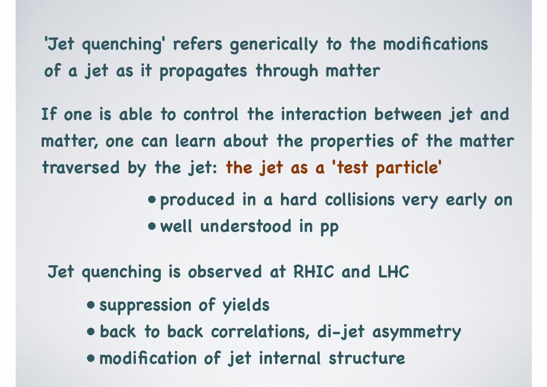
'Jet quenching' refers generically to the modifications of a jet as it propagates through matter

If one is able to control the interaction between jet and matter, one can learn about the properties of the matter traversed by the jet: the jet as a 'test particle'

• produced in a hard collisions very early on• well understood in pp

Jet quenching is observed at RHIC and LHC

• suppression of yields• back to back correlations, di-jet asymmetry• modification of jet internal structure

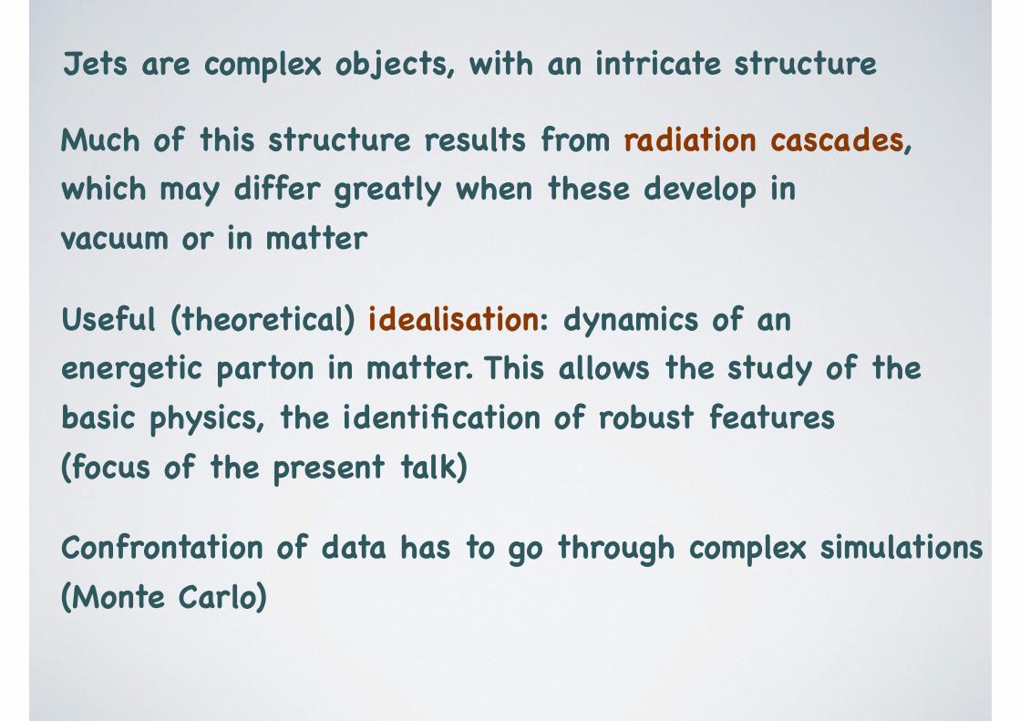
Jets are complex objects, with an intricate structure

Much of this structure results from radiation cascades, which may differ greatly when these develop in vacuum or in matter

Useful (theoretical) idealisation: dynamics of an energetic parton in matter. This allows the study of the basic physics, the identification of robust features (focus of the present talk)

Confrontation of data has to go through complex simulations (Monte Carlo)

Prejudices about the matter probed by jets in heavy ion collisions

- strongly coupled liquid without well defined quasiparticles

- weakly coupled quark-gluon plasma

In fact, most descriptions rely mainly on the assumption that the interaction between the plasma and the jet is weak and can be treated (semi) perturbatively

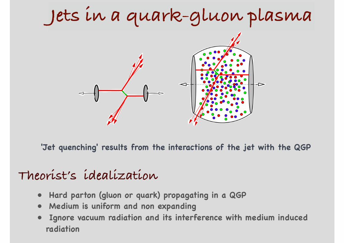
Jets in a quark-gluon plasma

'Jet quenching' results from the interactions of the jet with the QGP

Theorist’s idealization• Hard parton (gluon or quark) propagating in a QGP• Medium is uniform and non expanding• Ignore vacuum radiation and its interference with medium induced

radiation

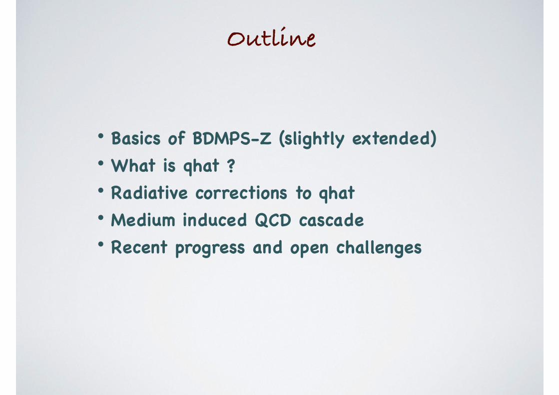
Outline

• Basics of BDMPS-Z (slightly extended)• What is qhat ?• Radiative corrections to qhat• Medium induced QCD cascade• Recent progress and open challenges

Basics of BDMPS-Z[Baier, Dokshitzer, Mueller, Peigné, Schiff (1995-2000) Zakharov (1996)]

(slightly extended)

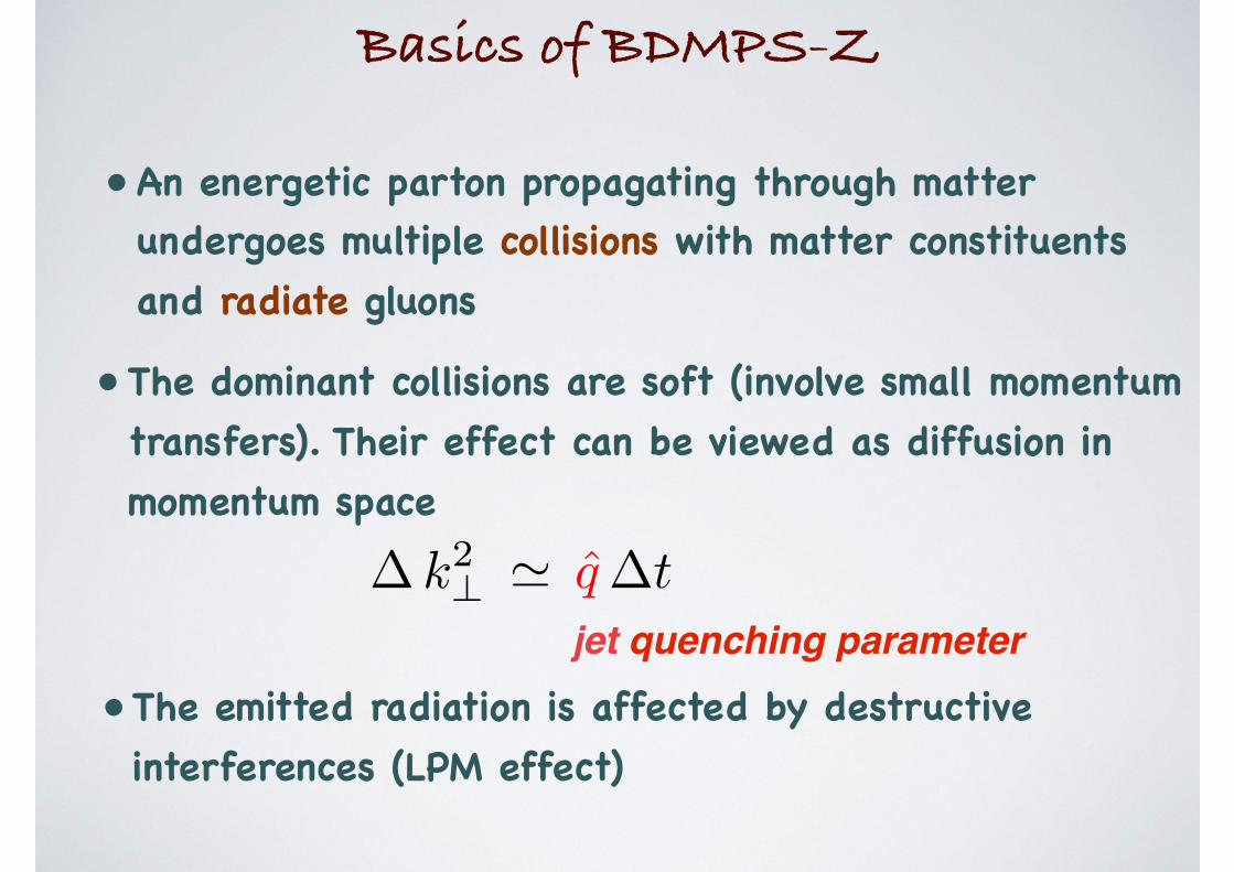
Basics of BDMPS-Z

• An energetic parton propagating through matter undergoes multiple collisions with matter constituents and radiate gluons

• The dominant collisions are soft (involve small momentum transfers). Their effect can be viewed as diffusion in momentum space

� k2? ' q �t

jet quenching parameter• The emitted radiation is affected by destructive interferences (LPM effect)

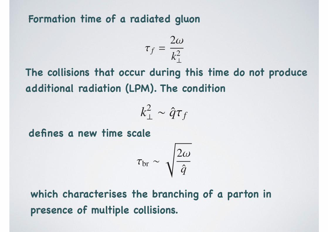
Formation time of a radiated gluon

⌧ f =2!k2?

The collisions that occur during this time do not produce additional radiation (LPM). The condition

k2? ⇠ q⌧ f

defines a new time scale

⌧br ⇠s

2!q

which characterises the branching of a parton in presence of multiple collisions.

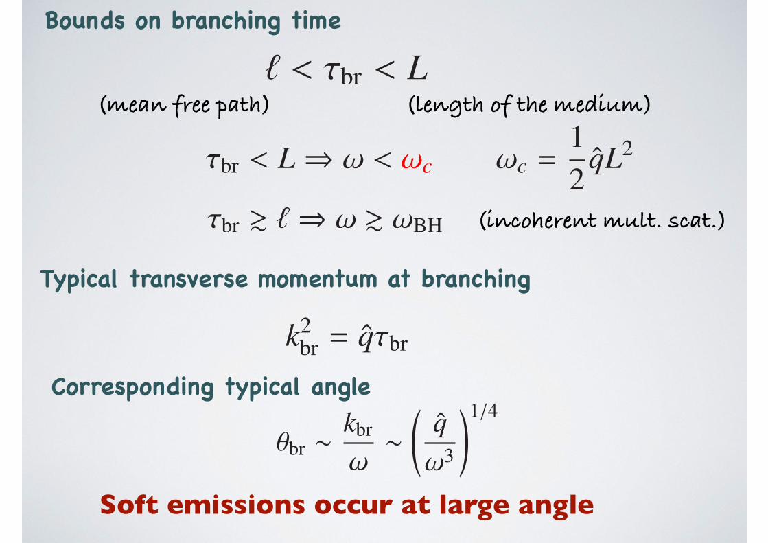
` < ⌧br < L

⌧br < L) ! < !c !c =12

qL2

⌧br & ` ) ! & !BH

k2br = q⌧br

✓br ⇠kbr

!⇠

q!3

!1/4

Soft emissions occur at large angle

(mean free path) (length of the medium)

Typical transverse momentum at branching

Corresponding typical angle

Bounds on branching time

(incoherent mult. scat.)

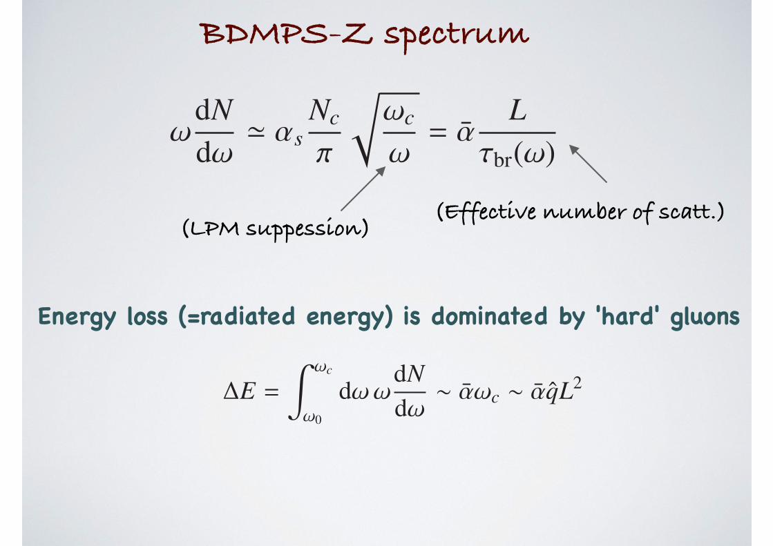
!dNd!' ↵s

Nc

⇡

r!c

!= ↵

L⌧br(!)

�E =Z !c

!0

d!!dNd!⇠ ↵!c ⇠ ↵qL2

BDMPS-Z spectrum

(LPM suppession)(Effective number of scatt.)

Energy loss (=radiated energy) is dominated by 'hard' gluons

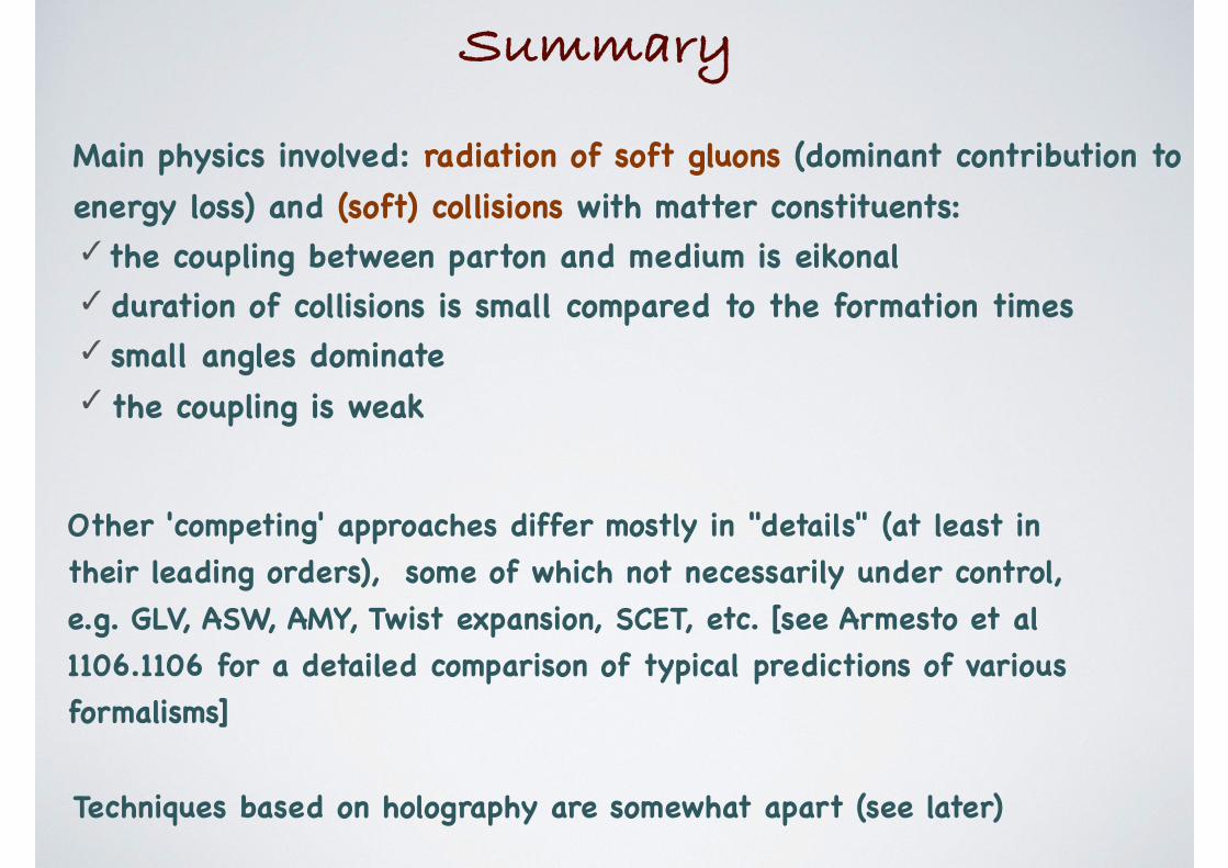
Summary

Main physics involved: radiation of soft gluons (dominant contribution to energy loss) and (soft) collisions with matter constituents: ✓ the coupling between parton and medium is eikonal✓ duration of collisions is small compared to the formation times✓ small angles dominate✓ the coupling is weak

Other 'competing' approaches differ mostly in "details" (at least in their leading orders), some of which not necessarily under control, e.g. GLV, ASW, AMY, Twist expansion, SCET, etc. [see Armesto et al 1106.1106 for a detailed comparison of typical predictions of various formalisms]

Techniques based on holography are somewhat apart (see later)

What is ?q

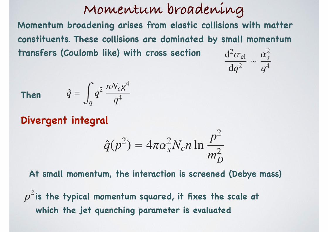
Momentum broadening arises from elastic collisions with matter constituents. These collisions are dominated by small momentum transfers (Coulomb like) with cross section d2�el

dq2 ⇠↵2

s

q4

Divergent integral

q(p2) = 4⇡↵2s Ncn ln

p2

m2D

p2 is the typical momentum squared, it fixes the scale at which the jet quenching parameter is evaluated

Momentum broadening

At small momentum, the interaction is screened (Debye mass)

q =Z

qq2 nNcg4

q4Then

Momentum broadening

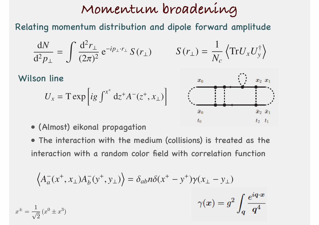
Wilson line

Relating momentum distribution and dipole forward amplitude

• (Almost) eikonal propagation• The interaction with the medium (collisions) is treated as theinteraction with a random color field with correlation function

dNd2 p?

=

Zd2r?(2⇡)2 e�ip?·r? S (r?) S (r?) =

1Nc

DTrUxU†y

E

Ux = T expigR x+ dz+A�(z+, x?)

�

DA�a (x+, x?)A�b (y+, y?)

E= �abn�(x+ � y+)�(x? � y?)

BRIEF ARTICLE

THE AUTHOR

ωdN

dω≃

αsNc

π

!

ωc

ω≡ α

!

ωc

ω= α

L

τbr(ω)

ωBH

≪ ω ! ωc

x± =

1√2(x0 ± x

3)

1

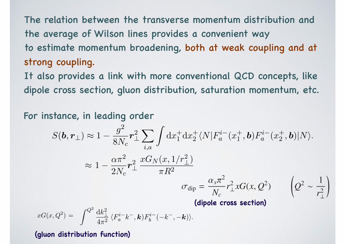
The relation between the transverse momentum distribution and the average of Wilson lines provides a convenient wayto estimate momentum broadening, both at weak coupling and at strong coupling.It also provides a link with more conventional QCD concepts, like dipole cross section, gluon distribution, saturation momentum, etc.

For instance, in leading order

13 Relating the dipole cross section to the gluon density

The calculation will assume the field of the nucleon to be weak, and we shall proceed with

a perturbative calculation. The leading order contribution is that of second order in g.

The first order would involve the average color field of the nucleon, which vanishes by color

neutrality. It is represented by the gauge field A�. The dipole is moving in the positive

direction. By expanding the Wilson lines we get

U(x) = T exp

⇢ig

Zdx+A�

a (x+,x) ta

�

' 1 + ig

Zdx+A�

a (x+,x) ta

�g2

2

Zdx+1

Zdx+2 T

hA�

a (x+1 ,x) t

aA�b(x+2 ,x) t

b

i+ · · · ,

(13.1)

and similarly for U †(y?) Should we have a ta in U † to represent the antiquark? When

calculating U †U , we get two terms that involve T products, for instance

g2

2

�ab2

Zdx+1 dx

+2

⌦TA�

a (x+1 ,x)A

�a (x

+2 ,x)

↵, (13.2)

where we have used Trtatb = �ab/2. And one term involving the square of two leading

order amplitudes

g2�ab2

Zdx+1 dx

+2 hN |A�

a (x+1 ,y?)A

�a (x

+2 ,x)|Ni (13.3)

Assuming the amplitude to be purely absorptive, we can ignore the T -product To be better

explained. Why is S real ? Origin of absorption ?. Then we can rewrite S(b, r?) as

1 +g2

2

X

a

⇢Zdx+1 dx

+2 hN |A�

a (x+1 ,y)A

�a (x

+2 ,x)

�1

2A�

a (x+1 ,y)A

�a (x

+2 ,y)�

1

2A�

a (x+1 ,x)A

�a (x

+2 ,x)|Ni

�. (13.4)

We next expand, A�a (x

+1 ,x) = A�

a (x+1 , b) +

r2 ·rA�

a (x+1 , b), and set F i�

a = riA�a . We get

S(b, r?) ⇡ 1� g2

8Nc

r2?X

i,a

Zdx+1 dx

+2 hN |F i�

a (x+1 , b)Fi�a (x+2 , b)|Ni. (13.5)

Note that the factor 1/Nc is coming from the trace in the fundamental representation:

we calculate (1/Nc)Tr(1� g2tatb · · · ). We have used Trtatb = tF = 1/2. The changes for a

gluon dipole involves changing the matrices ta into matrices of the adjoint representation,

ta ! T a. We have TrT aT b = tA = Nc. Furthermore the trace is now to be divided by

N2c � 1. Collecting all the factors, one finds that the quadratic term for gluon is obtained

from the quark contribution by multiplying by the factor

tAN2

c � 1

Nc

tF=

2N2c

N2c � 1

=CA

CF

, (13.6)

– 34 –

be calculated explicitly. We haveZ

d2r?

ZQ

2dk2?4⇡2

eik?·(x?�y?)

=1

2⇡2

Zrdr

ZQ

0dk k

Z 2⇡

0d✓ eikr cos ✓

✓Z 2⇡

0d✓ eikr cos ✓ = 2⇡J0(x)

◆

=1

⇡

Zrdr

ZQ

0dk kJ0(kr)

✓ZQ

0duuJ0(u) = QJ1(Q)

◆

=1

⇡

Zdr

rQrJ1(Qr) =

1

⇡

ZduJ1(u). (13.12)

If the integration is carried from 0 to infinity, one recovers the previous result. That is,RduJ1(u) = 1. We may also observe that the integral is dominated by values of u of order

unity. In fact,Rx0

0 duJ1(u) = 1, for x0 ⇡ 2.4 where x0 is the first zero of J0(x).

In summary, taking all this into account, one can rewrite the expression above asZ

Q2dk2?4⇡2

hF i�a (k�,k)F i�

a (�k�,�k)i

⇡ ⇡R2

⇡

Zdx+dy+ eik

�(x+�y+)hF i�

a (x+, b)F i�a (y+, b)i

⇡ xGN (x, 1/r2?). (13.13)

One can verify that this calculation reproduces the result for the distribution function of

a single quark (in a color singlet system). We have indeed in this case

ZQ

2dk2?4⇡2


a (�k�,�k)i

⇡ ⇡R2

⇡

Zdx+dy+ e�ik

�(x+�y+)hF i�

a (x+, b)F i�a (y+, b)i

⇡ ⇡R2

⇡(N2

c � 1)

Zdx+µ(x+)

Z

k

1

k2?

=⇡R2

⇡(N2

c � 1)g2

2Nc

1

⇡R2

Z

k

1

k2?=

↵CF

⇡

Zdk2?k2?

,

(13.14)

which is indeed the expected result.

It follows that we can write the dipole S-matrix as follows

S(b, r?) ⇡ 1� g2

8Nc

r2?X

i,a

Zdx+1 dx

+2 hN |F i�

a (x+1 , b)Fi�a (x+2 , b)|Ni

⇡ 1� g2

8Nc

r2?⇡

⇡R2xGN (x, 1/r2?)

⇡ 1� ↵⇡2

2Nc

r2?xGN (x, 1/r2?)

⇡R2. (13.15)

At the present level of approximation the resulting gluon distribution does not depend

on x. To be discussed.

– 36 –

that is the factor g2/(8Nc) is changed into g2Nc/(4(N2c � 1)).

We now argue that this expression is related to the gluon distribution function A

REVOIR aussi signe de la transforme de Fourier. We have indeed, for the unintegrated

distribution function (see below)


b(�k�,�k)i = 4⇡2

k2?

'(x,k?). (13.7)

with k� = xP�, and


b(�k�,�k)i

=

Zdx+dy+

Z

x,yeik

�(x+�y+)e�ik?·(x?�y?)hF i�

a (x+,x)F i�b

(y+,y)i.

(13.8)

The gluon density is given by

xG(x,Q2) =

ZQ

2dk2?k2?

'(x, k2?)

=

ZQ

2dk2?4⇡2

hF i�a k�,k)F i�

b(�k�,�k)i. (13.9)

Consider then the integral

ZQ

2dk2?4⇡2


b(�k�,�k)i

=

ZQ

2dk2?4⇡2

Zdx+dy+

Z

x,yeik

�(x+�y+)e�ik?·(x?�y?)hF i�

a (x+,x)F i�b

(y+,y)i.

(13.10)

We can writeRx,y =

Rr?,b. The integration over b gives a factor ⇡R2. The integration

over x� y is limited to |x� y| . 1/Q. We assume that Q is large enough so that r?, the

size of the dipole is small compared to the size of the nucleon, and that over that size the

correlator does not vary much. Under these conditions, one can simplify the calculation of

the integral over k? and r?. In fact, assuming rotational invariance (independence of the

correlator on the direction of k?), we can write

ZQ

2dk2?4⇡2

eik?·(x?�y?) �!Z

Q2

2d2k?(2⇡)3

eik?·(x?�y?) =1

⇡�(x� y), (13.11)

in the limit where Q ! 1. The remaining integral over r? is then trivial, and the net

result of the combined integrations over k? and r? is simply 1/⇡. This integral can in fact

– 35 –

that is the factor g2/(8Nc) is changed into g2Nc/(4(N2c � 1)).

We now argue that this expression is related to the gluon distribution function A

REVOIR aussi signe de la transforme de Fourier. We have indeed, for the unintegrated

distribution function (see below)


b(�k�,�k)i = 4⇡2

k2?

'(x,k?). (13.7)

with k� = xP�, and


b(�k�,�k)i

=

Zdx+dy+

Z

x,yeik

�(x+�y+)e�ik?·(x?�y?)hF i�

a (x+,x)F i�b

(y+,y)i.

(13.8)

The gluon density is given by

xG(x,Q2) =

ZQ

2dk2?k2?

'(x, k2?)

=

ZQ

2dk2?4⇡2

hF i�a k�,k)F i�

b(�k�,�k)i. (13.9)

Consider then the integral

ZQ

2dk2?4⇡2


b(�k�,�k)i

=

ZQ

2dk2?4⇡2

Zdx+dy+

Z

x,yeik

�(x+�y+)e�ik?·(x?�y?)hF i�

a (x+,x)F i�b

(y+,y)i.

(13.10)

We can writeRx,y =

Rr?,b. The integration over b gives a factor ⇡R2. The integration

over x� y is limited to |x� y| . 1/Q. We assume that Q is large enough so that r?, the

size of the dipole is small compared to the size of the nucleon, and that over that size the

correlator does not vary much. Under these conditions, one can simplify the calculation of

the integral over k? and r?. In fact, assuming rotational invariance (independence of the

correlator on the direction of k?), we can write

ZQ

2dk2?4⇡2

eik?·(x?�y?) �!Z

Q2

2d2k?(2⇡)3

eik?·(x?�y?) =1

⇡�(x� y), (13.11)

in the limit where Q ! 1. The remaining integral over r? is then trivial, and the net

result of the combined integrations over k? and r? is simply 1/⇡. This integral can in fact

– 35 –

�dip =↵s⇡2

Ncr2?xG(x,Q2)

Q2 ⇠ 1

r2?

!

(dipole cross section)

(gluon distribution function)

Multiple scattering (exponentiation of the lowest order result)

Q2s = qL

Q2s =

2⇡2↵s

Nc

AxGN(x, 1/r2?)

⇡R2

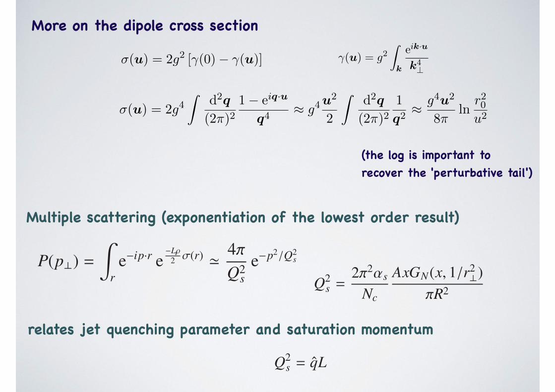
More on the dipole cross section

10 Momentum broadening

In the study of momentum broadening, we define

�(u) = 2g2 [�(0)� �(u)] , �(u) = g2Z

k

eik·u

k4?

(10.1)

that is

�(u) = 2g4Z

k

1� eik·r?

k4?

. (10.2)

The factor 2 in the definition of �(u) comes from the fact that there are initially four

diagrams, two contributing to �(0) and two contributing to �(u). The integral in the

definition of �(u) is divergent at small momenta. It may be calculated by including an

infrared regulator, for instance adding a screening mass (see subsection 10.4). We get then

�(u) = 2g4Z

d2q

(2⇡)21� eiq·u

(q2 +m20)

2, (10.3)

so that

�(l) =

Zd2u e�il·u�(u) = �2

g4

(l2 +m20)

2+ 2g4�(l)

Zd2q

(2⇡)21

(q2 +m20)

2

= �V (l) + �(l)

Z

qV (q). (10.4)

We have set

V (q) ⌘ 2g4

(q2 +m20)

2. (10.5)

10.1 The dipole S-matrix

The S-matrix for the dipole in the representation R is of the form

S(b, r?) = exp

⇢�µCRg

2Z

k

1� eik·r?

k4?

�

= exp

⇢�1

2µCR�(u)

�

= exp

⇢�1

4CRL⇢�(u)

�

(10.6)

where L is the distance travelled by the quark dipole in the nucleus, and ⇢ is the density

of nucleons per unit volume (we have assumed that A = ⇢L⇡R2, ignoring dependence on

the impact parameter, i.e., a uniform density in the disk of radius R). Also, we have used

µ =g2

2Nc

1

⇡R2Nval =

g2

2

A

⇡R2. (10.7)

– 24 –

10 Momentum broadening

In the study of momentum broadening, we define

�(u) = 2g2 [�(0)� �(u)] , �(u) = g2Z

k

eik·u

k4?

(10.1)

that is

�(u) = 2g4Z

k

1� eik·r?

k4?

. (10.2)

The factor 2 in the definition of �(u) comes from the fact that there are initially four

diagrams, two contributing to �(0) and two contributing to �(u). The integral in the

definition of �(u) is divergent at small momenta. It may be calculated by including an

infrared regulator, for instance adding a screening mass (see subsection 10.4). We get then

�(u) = 2g4Z

d2q

(2⇡)21� eiq·u

(q2 +m20)

2, (10.3)

so that

�(l) =

Zd2u e�il·u�(u) = �2

g4

(l2 +m20)

2+ 2g4�(l)

Zd2q

(2⇡)21

(q2 +m20)

2

= �V (l) + �(l)

Z

qV (q). (10.4)

We have set

V (q) ⌘ 2g4

(q2 +m20)

2. (10.5)

10.1 The dipole S-matrix

The S-matrix for the dipole in the representation R is of the form

S(b, r?) = exp

⇢�µCRg

2Z

k

1� eik·r?

k4?

�

= exp

⇢�1

2µCR�(u)

�

= exp

⇢�1

4CRL⇢�(u)

�

(10.6)

where L is the distance travelled by the quark dipole in the nucleus, and ⇢ is the density

of nucleons per unit volume (we have assumed that A = ⇢L⇡R2, ignoring dependence on

the impact parameter, i.e., a uniform density in the disk of radius R). Also, we have used

µ =g2

2Nc

1

⇡R2Nval =

g2

2

A

⇡R2. (10.7)

– 24 –

(Note that the factor g2 is included in the cross section.)

Interpreting S2 = |S|2 (S is real) as a survival probability, given in case of independent

multiple scattering by the generic form |S|2 = exp (�⇢L�), we may then identify the

elementary cross section �:

� =CR

2�(u). (10.8)

10.2 Expression in terms of the saturation momentum

A good approximation is obtained by using the small u expansion of �(u). We have

�(u) = 2g4Z

d2q

(2⇡)21� eiq·u

q4⇡ g4

u2

2

Zd2q

(2⇡)21

q2⇡ g4u2

8⇡ln

r20u2

, (10.9)

where the two scales in the log are the confinement scale r0 and the size u ⌧ r0 of the

dipole. The S-matrix for a gluon dipole can then be written as

S(b, r?) = exp

⇢�1

4CA�(r?)L⇢

�

= exp

⇢�1

4r2?Q

2s

�, (10.10)

where

Q2s =

4⇡2↵Nc

N2c � 1

L⇢xGN (x,Q2s) . (10.11)

Note that the log hidden in the gluon distribution function should be evaluated at a scale

⇠ 1/r?. But according to Eq. (10.10), this is also Qs. The same expression holds for a

quark dipole after substituting Q2s with

Q2s =

4⇡2↵CF

N2c � 1

L⇢xGN (x, Q2s) =

2⇡2↵

Nc

L⇢xGN (x, Q2s). (10.12)

Note that, if one ignores the change of scales in the logarithms, we have

Q2s

Q2s

=CF

CA

. (10.13)

10.3 Relation to momentum broadening

The jet quenching parameter q is obtained as

q0 = �Ncn

2

Z

ll2 �(l) = Ncng

4Z

l

l2

(l2 +m20)

2. (10.14)

In this expression, n is the density of nucleon per unit volume (see below).

For a parton in representation R

qR = ⇢4⇡2↵CR

N2c � 1

xG(x, qRL). (10.15)

– 25 –

P(p?) =Z

re�ip·r e

�L⇢2 �(r) ' 4⇡

Q2s

e�p2/Q2s

(the log is important to recover the 'perturbative tail')

relates jet quenching parameter and saturation momentum

Summary

The jet quenching parameter is a multifaceted object

• It plays the role of a (momentum dependent) diffusion constant in momentum space, reflecting the effects of multiple soft collisions

• It controls both momentum broadening and energy loss• It is related (in lowest orders) to the total cross section for

a dipole propagating through matter• It is related to the gluon distribution• It is related to the saturation momentum

qRadiative corrections to

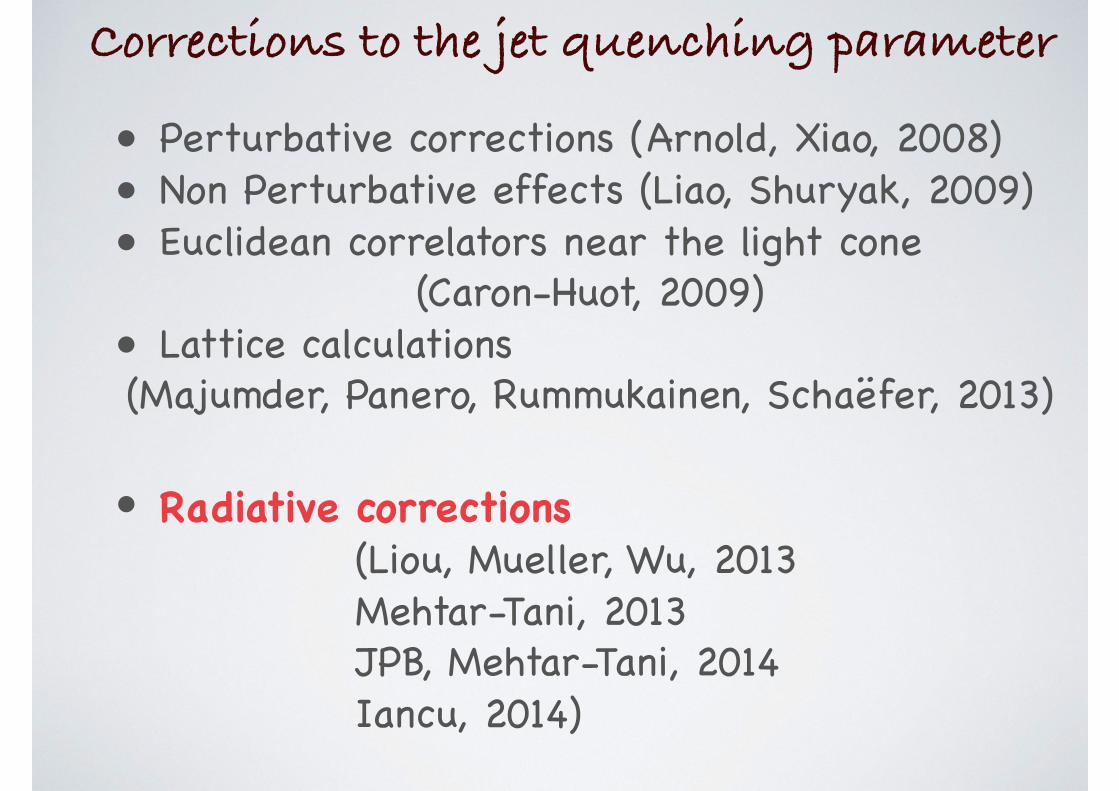
• Perturbative corrections (Arnold, Xiao, 2008)• Non Perturbative effects (Liao, Shuryak, 2009)• Euclidean correlators near the light cone

(Caron-Huot, 2009) • Lattice calculations (Majumder, Panero, Rummukainen, Schaëfer, 2013)

• Radiative corrections(Liou, Mueller, Wu, 2013Mehtar-Tani, 2013 JPB, Mehtar-Tani, 2014Iancu, 2014)

Corrections to the jet quenching parameter

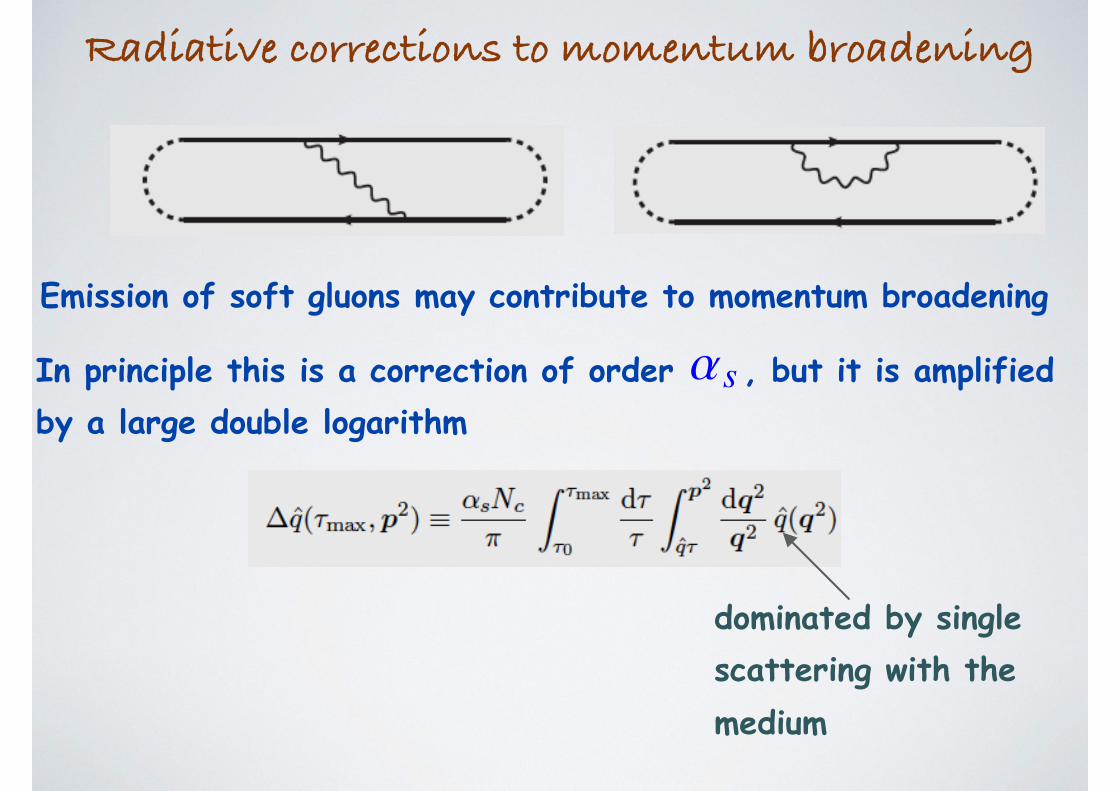
Radiative corrections to momentum broadening

In principle this is a correction of order , but it is amplified by a large double logarithm

Emission of soft gluons may contribute to momentum broadening

↵s

dominated by single scattering with the medium

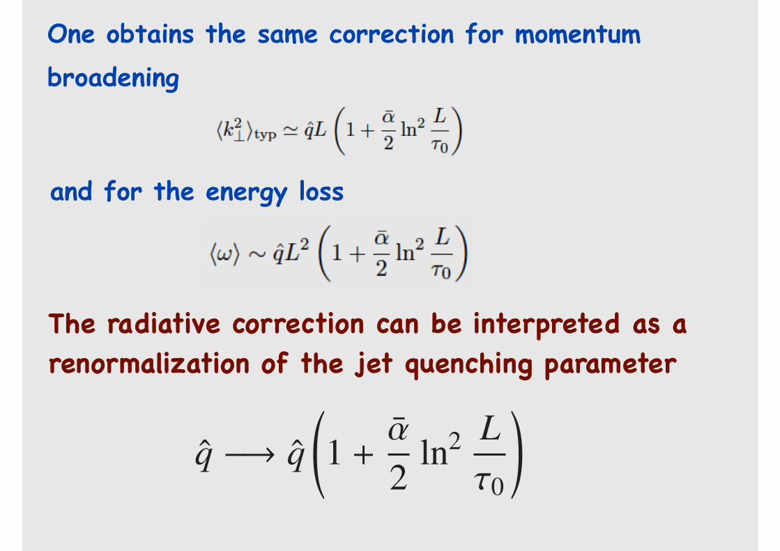
One obtains the same correction for momentum broadening

and for the energy loss

q �! q 1 +↵

2ln2 L⌧0

!

The radiative correction can be interpreted as a renormalization of the jet quenching parameter

(Y. M-T, 2013)

The double log corrections cane be resummed assuming strong ordering in formation times and transverse momenta

This yields new power laws (anomalous dimension)

226 J.-P. Blaizot, Y. Mehtar-Tani / Nuclear Physics A 929 (2014) 202–229

mD ≪ q1 ≪ ... ≪ qn ≡ k. The difference with the standard Double-Logarithmic Approximation (DLA) lies in the limits of the logarithmic phase-space set by the LPM effect, namely multiple scatterings. In the DLA, only the single scattering contributes, which imposes to the formation time of the fluctuation to be smaller than the BDMPS formation time, or in terms of our trans-verse momentum variables, q2 ≫ q0τ . The following equation resums the double logarithmic corrections to all orders

∂ q(τ,k2)

∂ ln τ=

k2!

qτ

d q2

q2 α(q)q"τ,q2# (85)

with some initial condition q(τ0, k). We have let the coupling running at the transverse scale q . Note the lower limit of the q integration which accounts for the boundary between single-scattering and multiple-scatterings. The important feature of this equation is it predicts the evolution of the jet-quenching parameter from an initial condition q0, which can be computed e.g. on the lattice, or to leading order in αs , which implies q(τ0) ≡ q0 as given by the leading order result (23). The τ0 cut-off that was introduced to cut the logarithmic divergence in the radiative corrections, can be seen as a factorization scale.

The complete solution of the 2-dimensional evolution equation (85) is beyond the scope of this paper.7 Let us simply recall the solution derived in [11] for the p⊥-broadening in the case where q0 = q(τ0) is constant and for a final τ = L and k2 = q0L, merging the 2 independent variables at the end of the evolution. The solution reads

q(L) = 1√α

I1

$2√

α lnL

τ0

%q(τ0). (86)

For large L, the quenching parameter scales like q(L) ∼Lγ , with the anomalous

γ = 2√

α.

Interestingly, the resummation of large double logarithms modifies the scaling of the energy loss with L, ⟨ω⟩ ∼ L2+γ , leading to a result that falls between the standard small coupling result, ⟨ω⟩ ∼L2 and the strong coupling result obtained with the help of the AdS–CFT correspondencein N = 4 SYM theory, ⟨ω⟩ ∼L3 [18].

Acknowledgements

We thank F. Dominguez, E. Iancu, A.H. Mueller and B. Wu for numerous discussions on some of the issues discussed in this paper. E. Iancu has recovered some of the results of this paper form the point of view of evolution equations [19]. Special thanks go to him for persuasive encouragements to speed up the writing of this paper. This research is supported by the European Research Council under the Advanced Investigator Grant ERC-AD-267258.

Appendix A. Calculational details

In this appendix, we provide some additional details on the calculations that lead to the expressions in the main text, in particular the expression (36) for the modification, due to a

7 During the editorial process of this article, the solution of Eq. (84) has been discussed in Ref. [20].

226 J.-P. Blaizot, Y. Mehtar-Tani / Nuclear Physics A 929 (2014) 202–229

mD ≪ q1 ≪ ... ≪ qn ≡ k. The difference with the standard Double-Logarithmic Approximation (DLA) lies in the limits of the logarithmic phase-space set by the LPM effect, namely multiple scatterings. In the DLA, only the single scattering contributes, which imposes to the formation time of the fluctuation to be smaller than the BDMPS formation time, or in terms of our trans-verse momentum variables, q2 ≫ q0τ . The following equation resums the double logarithmic corrections to all orders

∂ q(τ,k2)

∂ ln τ=

k2!

qτ

d q2

q2 α(q)q"τ,q2# (85)

with some initial condition q(τ0, k). We have let the coupling running at the transverse scale q . Note the lower limit of the q integration which accounts for the boundary between single-scattering and multiple-scatterings. The important feature of this equation is it predicts the evolution of the jet-quenching parameter from an initial condition q0, which can be computed e.g. on the lattice, or to leading order in αs , which implies q(τ0) ≡ q0 as given by the leading order result (23). The τ0 cut-off that was introduced to cut the logarithmic divergence in the radiative corrections, can be seen as a factorization scale.

The complete solution of the 2-dimensional evolution equation (85) is beyond the scope of this paper.7 Let us simply recall the solution derived in [11] for the p⊥-broadening in the case where q0 = q(τ0) is constant and for a final τ = L and k2 = q0L, merging the 2 independent variables at the end of the evolution. The solution reads

q(L) = 1√α

I1

$2√

α lnL

τ0

%q(τ0). (86)

For large L, the quenching parameter scales like q(L) ∼Lγ , with the anomalous

γ = 2√

α.

Interestingly, the resummation of large double logarithms modifies the scaling of the energy loss with L, ⟨ω⟩ ∼ L2+γ , leading to a result that falls between the standard small coupling result, ⟨ω⟩ ∼L2 and the strong coupling result obtained with the help of the AdS–CFT correspondencein N = 4 SYM theory, ⟨ω⟩ ∼L3 [18].

Acknowledgements

We thank F. Dominguez, E. Iancu, A.H. Mueller and B. Wu for numerous discussions on some of the issues discussed in this paper. E. Iancu has recovered some of the results of this paper form the point of view of evolution equations [19]. Special thanks go to him for persuasive encouragements to speed up the writing of this paper. This research is supported by the European Research Council under the Advanced Investigator Grant ERC-AD-267258.

Appendix A. Calculational details

In this appendix, we provide some additional details on the calculations that lead to the expressions in the main text, in particular the expression (36) for the modification, due to a

7 During the editorial process of this article, the solution of Eq. (84) has been discussed in Ref. [20].

so that D�p2?E⇠ L1+� h�Ei ⇠ L2+�

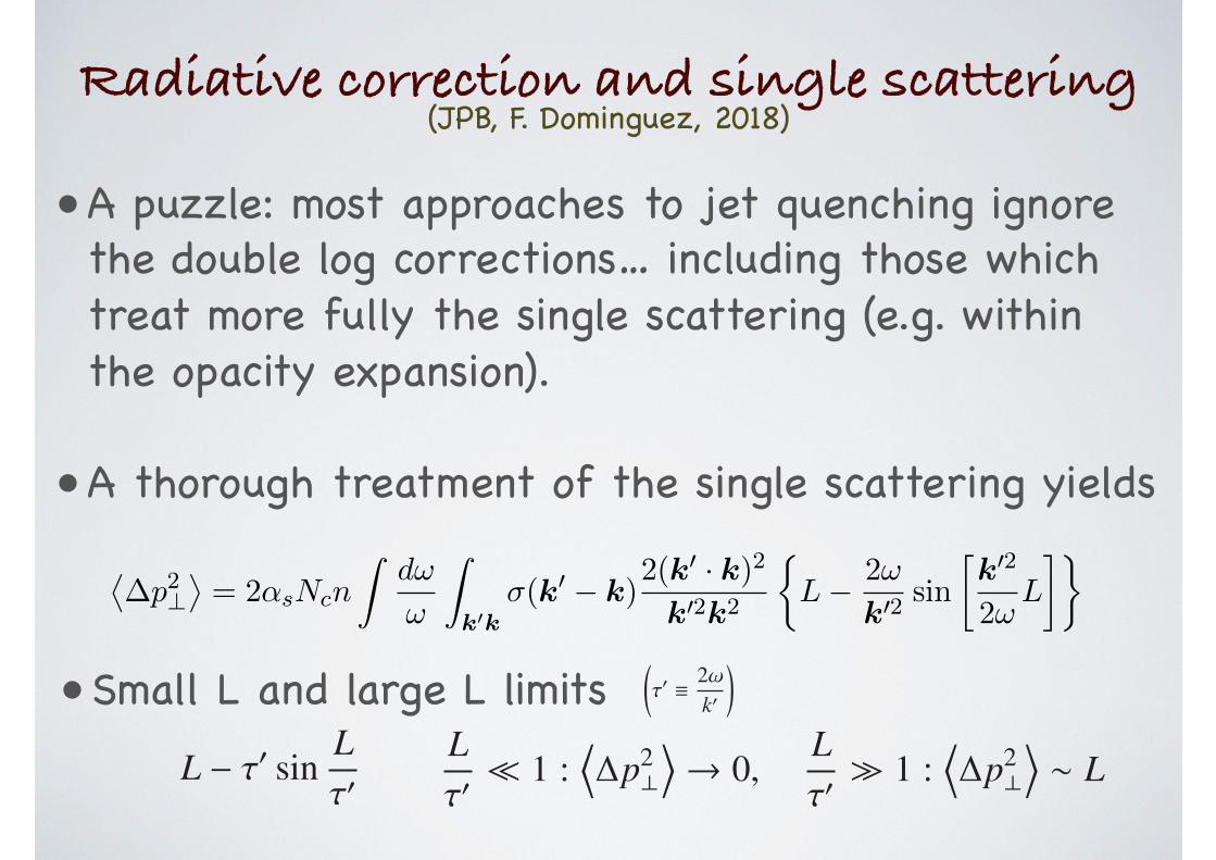
Radiative correction and single scattering

• A puzzle: most approaches to jet quenching ignore the double log corrections… including those which treat more fully the single scattering (e.g. within the opacity expansion).

• A thorough treatment of the single scattering yields

correspond to leading order momentum broadening of the hard gluon. The only terms survivingare those in which the medium interacts with a coherent system of two gluons. This is equivalentto the observation made after eq. (15) in the multiple scattering case, where it is noted thatthe broadening before and after the emission don’t play a role in the calculation of the radiativecorrection.

After accounting for these cancelations, the only surviving terms are those coming from thesine term in the last line of (26) and one of the terms in the second line of (28). These can becombined into the following expression:

⌦�p2?

↵= 2↵sNcn

Zd!

!

Z

k0k�(k0 � k)

2(k0 · k)2

k02k2

⇢L� 2!

k02 sin

k02

2!L

��. (31)

We have purposefully left the above formula without integration limits. The next sectionis devoted to limit the phase space region to the physically relevant cases and extracting thedouble logarithmic enhancement to the radiative correction.

4.2. Phase space region for double logarithmic contribution

The result from the previous section allows us to properly take into account the finitemedium e↵ects on the radiative correction. First of all, it is easy to see that the first term,proportional to the medium length, will show the same behavior as the double logarithm foundin the multiple scattering case. In fact, it coincides with the analysis performed in the Appendixof [2] where it is recognized that the double logarithmic radiative correction corresponds to thesingle scattering region. In summary,

Zd!

!

Z

k0k�(k0 � k)

2(k0 · k)2

k02k2=

Zd!

!

Z

lk�(l)

2((k + l) · k)2

(k + l)2k2

= 2

Zd!

!

Z

lk�(l)

(l · k)2 � l2k2

(k + l)2k2

⇠ �Z

d!

!

Z

k

1

k2

Z

ll2�(l). (32)

In going from the second to the third line above, we have recognized that the logarithmicenhancement is present for k � l. This sets the upper boundary for the l-integration, whichwill set the scale for q as in eq. (3).

Plugging the result of (32) back into (31) one gets the total contribution in the region wherethe sine function oscillates rapidly and therefore does not contribute. On the other hand, theoscillatory term induced by the finite size e↵ects will provide the missing boundary to thedouble logarithmic region. If the argument of the sine function is small, one can perform apower expansion, where the first non-zero contribution will be accompanied by an extra powerof momentum which kills the logarithmic contribution. In the relevant set of variables (!,k2),the new boundary is given by the condition

k2

2!L > 1. (33)

This new boundary e↵ectively replaces the one provided by the multiple scattering conditionfor the case in hand. The corresponding region is displayed in Fig. 7. It is easy to see thatthis condition is equivalent to the requirement that the formation time of the gluon is shorterthan the length of the medium, which is the condition used in [5, 4] in a multiple scatteringsetting to go beyond the region k2 ⇠ qL. It is important to emphasize that we have a clearderivation for this boundary for the single scattering case, which is the relevant physics for thislarge transverse momentum transfer regime.

The boundary given by eq. (33) does not completely replace the multiple scattering bound-ary. It is better seen as an upper boundary on the energy of the emitted gluon, and it allows

14

(JPB, F. Dominguez, 2018)

L � ⌧0 sinL⌧0

⌧0 ⌘ 2!

k0

!

• Small L and large L limitsL⌧0⌧ 1 :

D�p2?E! 0,

L⌧0� 1 :

D�p2?E⇠ L

Finite size effects versus multiple scattering

Figure 8: Phase space when single scattering dominates over multiple scattering

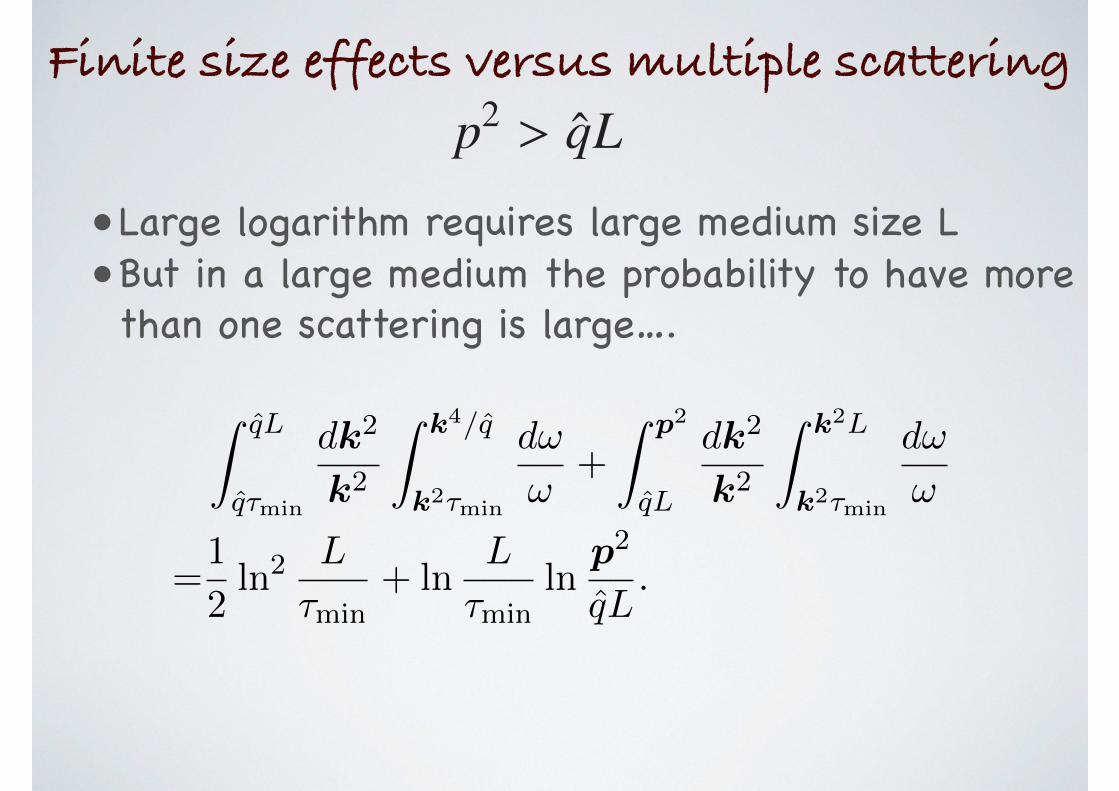
variable determining the size of the phase space region is the length of the medium, the doublelogarithmic contribution is enhanced only for a large medium, where the use of the singlescattering formalism is not justified. In other words, to have a large logarithmic contributionone needs to have a large medium, but in a large medium the probability to have more thanone scattering is large. This is the reason why the current formalisms used to describe jetquenching phenomena based on an opacity expansion don’t include such double logarithmiccontributions.

Now, taking into account that the two approximations studied in this paper are somewhatcomplementary and can be applied in di↵erent regions of phase space, it becomes important tounderstand how the multiple soft scattering and the single hard scattering approaches can becombined to obtain the most general region of phase space with a double logarithmic enhance-ment. When the corresponding phase space regions are superimposed, we see that the multiplescattering case is more restrictive at low transverse momentum while the single scattering caseis more restrictive at larger momentum. This might seem counterintuitive at first, since in prin-ciple through multiple scatterings the gluon could accumulate more transverse momentum, butwhat actually occurs is that in order to have a large momentum transfer one always needs (atleast) one hard kick from the medium.

It is easy to see that the corresponding boundaries for the two phase space regions intersectat k2 = qL. If the momentum scale p2 is smaller than this value then the multiple scatteringregime dominates. The medium is too long for the gluon to only scatter once. But if themomentum scale is larger, then there is a region of phase space that is only accesible through asingle hard scattering. This division is shown in Fig. 8 and the corresponding double integralis (for the case where the scale dependence of q is neglected)

Z qL

q⌧min

dk2

k2

Z k4/q

k2⌧min

d!

!+

Z p2

qL

dk2

k2

Z k2L

k2⌧min

d!

!

=1

2ln2

L

⌧min+ ln

L

⌧minln

p2

qL. (37)

It is the second term in (37) the one which shows the e↵ect of the single scattering case ontop of the already known multiple scattering contribution. It clearly shows how, for a fixed p2,changing the length of the medium could enhance one of the logarithms but would necessarilysuppress the other one. Moreover, the ratio of the two terms grows as the log of the length L,showing that for larger L the multiple scattering contribution is parametrically more important.

16

• Large logarithm requires large medium size L• But in a large medium the probability to have more than one scattering is large….

p2 > qL

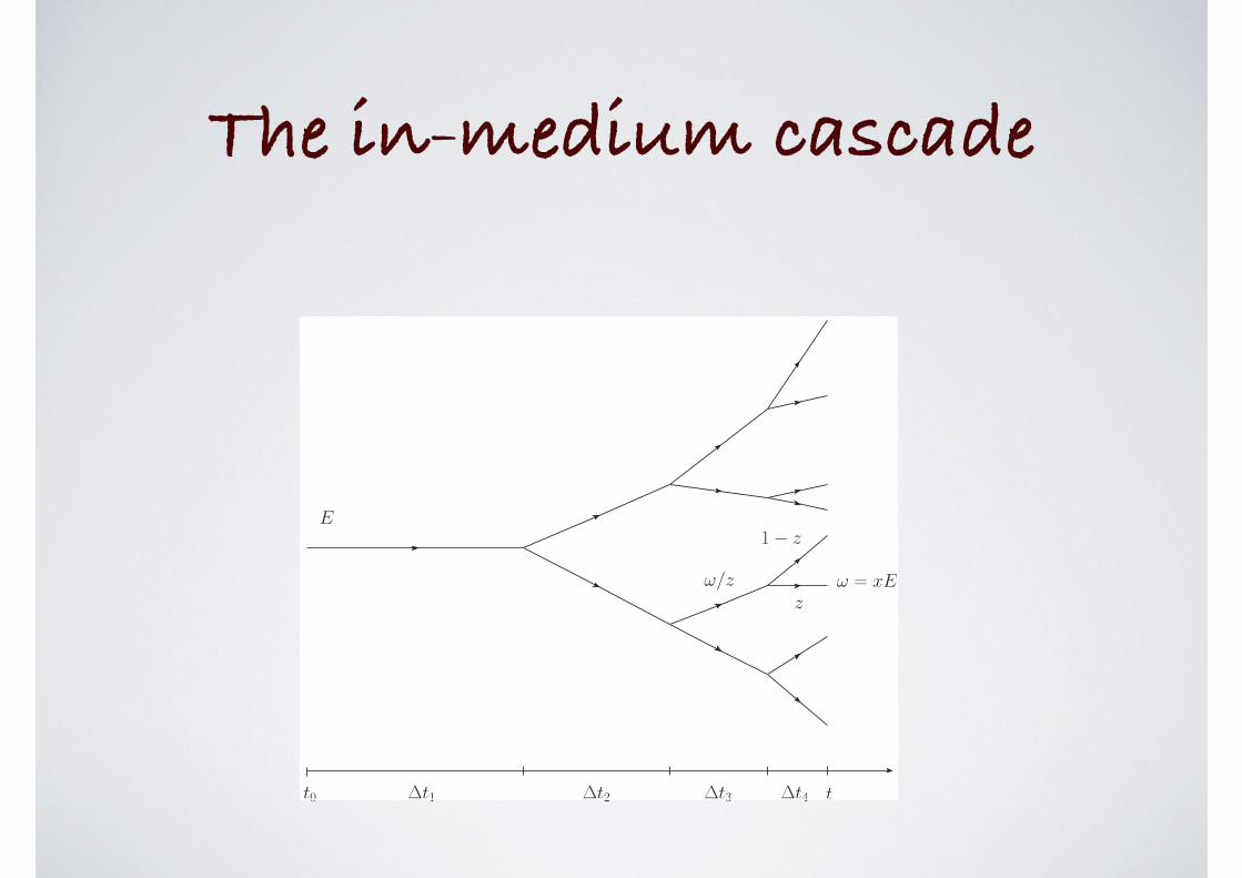
The in-medium cascade

E

! = xE

t

1 � z

z!/z

�t1 �t2 �t3 �t4t0

Figure 1: Illustration of a gluon cascade that is initiated by a gluon with energy E.

Four generations are displayed. The branching time �ti, that corresponds to the lifetime

of generation i, decreases after each branching as in a BDMPS cascade. The inclusive

distribution D(x, t) measures the probability to find in the cascade, at time t, a gluon

with energy xE. The rate equation (2.5) describes how this distribution evolves with time

t.

themselves radiate, eventually generating a cascade. Our goal is to study theaverage properties of such a cascade, focusing in this paper on the inclusivegluon distribution, integrated over transverse momentum,

D(x, t) ⌘ xdN

dx, (2.4)

where x = !/E is the energy fraction of the gluon observed at some time talong the cascade, cf. Fig 1 for an illustration. (D(x, t) can be viewed as anenergy density, with D(x, t) dx being the energy contained in modes2 withenergy fraction between x and x + dx.) As was shown in [21], D(x, t) obeys

2We use the term “mode” as a synonymous for radiated gluon throughout this paper

5

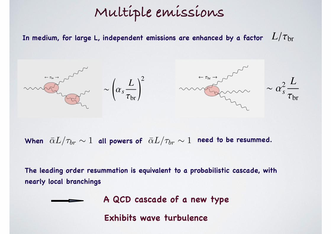
Multiple emissions

In medium, for large L, independent emissions are enhanced by a factor

When

BRIEF ARTICLE

THE AUTHOR

ωdN

dω≃

αsNc

π

!

ωc

ω≡ α

!

ωc

ω= α

L

τbr(ω)

ωBH

≪ ω ! ωc

x± =1√2(x0 ± x3)

∂µTµν = 0

∂µjµ = 0

T µν = (ϵ+ P )uµuν − Pgµν

jµ = nuµ

P =ϵ

3

ℓ ≪ αL

αL/τbr ∼ 1

1

all powers of

BRIEF ARTICLE

THE AUTHOR

ωdN

dω≃

αsNc

π

!

ωc

ω≡ α

!

ωc

ω= α

L

τbr(ω)

ωBH

≪ ω ! ωc

x± =1√2(x0 ± x3)

∂µTµν = 0

∂µjµ = 0

T µν = (ϵ+ P )uµuν − Pgµν

jµ = nuµ

P =ϵ

3

ℓ ≪ αL

αL/τbr ∼ 1

1

need to be resummed.

The leading order resummation is equivalent to a probabilistic cascade, with nearly local branchings

⇠ ↵s

L⌧br

!2

⇠ ↵2s

L⌧br

L/⌧br

A QCD cascade of a new type

Exhibits wave turbulence

carrying the fraction x of the initial energy, t⇤(x) = t⇤p

x. This time scaledecreases as x decreases, meaning that the rate of emission of soft gluonsis higher the softer the gluon: it follows that gluon splittings occur fasterand faster as one moves down the cascade, and, as a result, it takes a finitetime (of order t⇤) to transport a finite amount of energy form x = 1 downto x = 0 [20]. It is actually convenient to make this x-dependent time scalemore evident, and write Eq. (2.5) as

@

@tD(x, t) =

Z1

x

dz K(z)D (x/z, t)

t⇤(x/z)�

D (x, t)

t⇤(x)

Z1

0

dz zK(z) = I[D]. (2.8)

This form of the equation plays an important role in the foregoing analysis.In the present study, we shall use a simplified version of the reduced kernel

K(z) given in Eq. (2.7), namely

K(z) ⇡1

z3/2(1 � z)3/2, (2.9)

that is, we shall replace the smooth function f(z) in the numerator by 1. Themain motivation for using this simplified kernel is that one can then obtainthe solution analytically. This solution was already discussed in Ref. [5].Its explicit construction is presented in Appendix A (see Eq. (A.11)). Thesimplified kernel (2.9) captures properly the singular behaviors at z ! 0and z ! 1, while the smooth function f(z) plays a negligible role, as canbe verified through a comparison of the analytic solution with the numericalsolution obtained with the full kernel (2.7). We shall in fact verify throughoutthis work that the main qualitative features of the cascade are to a largeextent independent of the specific form of the (reduced) kernel.

Before we go into a discussion of the main features of this analytic so-lution, we wish to contrast this cascade of medium induced radiation withthe cascade of gluons emitted in vacuum by an energetic (o↵-shell) parton.This is described by the DGLAP evolution [13]. A simplified version of thecorresponding evolution equation for the inclusive one particle distributionreads

@

@tD(x, t) = ↵

Z1

x

dz

z(1 � z)D(x/z, t) � ↵

Z1

0

dz

1 � zD(x, t), (2.10)

where here the time variable is related to the virtuality Q2 of the emittingparton, t ⌘ ln Q2/Q2

0, and again only gluons are taken into account. This

8

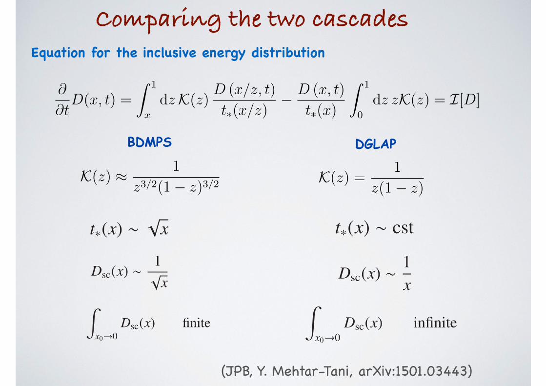
carrying the fraction x of the initial energy, t⇤(x) = t⇤p

x. This time scaledecreases as x decreases, meaning that the rate of emission of soft gluonsis higher the softer the gluon: it follows that gluon splittings occur fasterand faster as one moves down the cascade, and, as a result, it takes a finitetime (of order t⇤) to transport a finite amount of energy form x = 1 downto x = 0 [20]. It is actually convenient to make this x-dependent time scalemore evident, and write Eq. (2.5) as

@

@tD(x, t) =

Z1

x

dz K(z)D (x/z, t)

t⇤(x/z)�

D (x, t)

t⇤(x)

Z1

0

dz zK(z) = I[D]. (2.8)

This form of the equation plays an important role in the foregoing analysis.In the present study, we shall use a simplified version of the reduced kernel

K(z) given in Eq. (2.7), namely

K(z) ⇡1

z3/2(1 � z)3/2, (2.9)

that is, we shall replace the smooth function f(z) in the numerator by 1. Themain motivation for using this simplified kernel is that one can then obtainthe solution analytically. This solution was already discussed in Ref. [5].Its explicit construction is presented in Appendix A (see Eq. (A.11)). Thesimplified kernel (2.9) captures properly the singular behaviors at z ! 0and z ! 1, while the smooth function f(z) plays a negligible role, as canbe verified through a comparison of the analytic solution with the numericalsolution obtained with the full kernel (2.7). We shall in fact verify throughoutthis work that the main qualitative features of the cascade are to a largeextent independent of the specific form of the (reduced) kernel.

Before we go into a discussion of the main features of this analytic so-lution, we wish to contrast this cascade of medium induced radiation withthe cascade of gluons emitted in vacuum by an energetic (o↵-shell) parton.This is described by the DGLAP evolution [13]. A simplified version of thecorresponding evolution equation for the inclusive one particle distributionreads

@

@tD(x, t) = ↵

Z1

x

dz

z(1 � z)D(x/z, t) � ↵

Z1

0

dz

1 � zD(x, t), (2.10)

where here the time variable is related to the virtuality Q2 of the emittingparton, t ⌘ ln Q2/Q2

0, and again only gluons are taken into account. This

8

equation has the form of Eq. (2.8) if one identifies

1

t⇤(x)= ↵, (2.11)

and

K(z) =1

z(1 � z). (2.12)

Thus the DGLAP equation di↵ers from the BDMPS equation in two majoraspects. First, the kernel K(z) is less singular near z = 0 and z = 1. Second,the rate of successive branchings is independent of the parent energy, i.e., itis constant along the cascade. We shall see that the latter property is whatmakes the major di↵erence between the BDMPS and the DGLAP cascades.

2.1. The ideal medium-induced QCD cascade

We now return to the ideal medium-induced QCD cascade, and discussthe main features of the solution to Eq. (2.5) obtained with the simplifiedkernel (2.9). This solution reads (see Appendix A, Eq. (A.11))

D(x, ⌧) =⌧

px (1 � x)3/2

exp

✓�⇡

⌧ 2

1 � x

◆, ⌧ ⌘

t

t⇤. (2.13)

This solution exhibits two remarkable features: a peak near x = 1 asso-ciated with the leading particle, and a scaling behavior in 1/

px at small x

where the x dependence factorizes from the time dependence, i.e.

D(x, ⌧) ⇡⌧

px

e�⇡⌧2 . (2.14)

An illustration of this solution is given in Fig. 2, left panel. The energyof the leading particle, initially concentrated in the peak at x . 1, graduallydisappears into radiated soft gluons, and after a time t ⇠ t⇤ (i.e. ⌧ ⇠ 1/

p⇡ ⇡

0.5) most of the energy is to be found in the form of radiated soft (x . 0.1)gluons. This is also the time at which the peak corresponding to the leadingparticle disappears (see Fig. 2). These are the reasons that motivate callingt⇤ the stopping time. At the same time the occupation of the small x modesincreases (linearly) with time, keeping the characteristic form of the scalingspectrum. When the peak has disappeared, the cascade continues to lower

9

t⇤(x) ⇠ cstt⇤(x) ⇠p

x

Dsc(x) ⇠ 1px Dsc(x) ⇠ 1

xZ

x0!0Dsc(x) finite

Z

x0!0Dsc(x) infinite

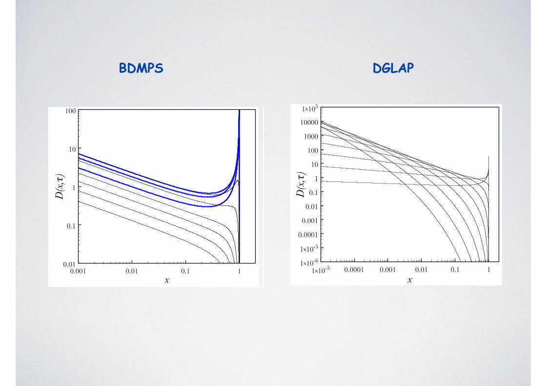
Comparing the two cascades

BDMPS DGLAP

(JPB, Y. Mehtar-Tani, arXiv:1501.03443)

Equation for the inclusive energy distribution

0.001 0.01 0.1 1x

0.01

0.1

1

10

100

D(x,!)

0.001 0.01 0.1 1x

0.01

0.1

1

10

100

D(x,!)

Figure 2: (Color online.) The function D(x, ⌧) (Eq. (2.13)) at various times. Left panel:

the filling of the modes, which proceeds till the disappearance of the leading particle

peak. The values of ⌧ are, for the thick (blue) curves, from bottom to top: 0.1, 0.2, 0.3

(during this stage the leading particle acts as a source for soft gluon radiation), and for

the thin (black) curves, from top to bottom: 0.5, 0.7, 0.9,1.0,1.1,1.2 (the leading parton

has exhausted its energy and the peak has disappeared, while energy continues to flow to

small x, the amount of energy in each mode decreasing exponentially fast). Right panel:

energy is constantly injected into the system by a source located at x = 1 (see Eq. (2.21)).

After a transitory regime, characterized by a uniform increase with time of the scaling

spectrum, the system reaches a steady state. The values of ⌧ are, from bottom to top:

0.1,0.2,0.3, 0.4, 0.5, 0.6,0.7,0.8,0.9,1.0.

x, causing a uniform, shape conserving, decrease of the occupations, and aflow of energy towards small x that we now analyze.

Energy conservation is explicitly implemented in Eq. (2.5) at the level ofindividual splittings. To see how this conservation law manifests itself moreglobally, it is useful to consider the flux of energy, F(x0, ⌧), towards valuesof x smaller than a value x0. This is defined by

F(x0, ⌧) = �@E(x0, ⌧)

@⌧, E(x0, ⌧) ⌘

Z1

x0

dxD(x, ⌧), (2.15)

where E(x0, ⌧) is the amount of energy contained in the modes with x >x0, and F(x0, ⌧) is counted positively for energy moving to values of x <x0 (hence the minus sign in the definition of F . These quantities can becalculated explicitly. We have for instance

E(x0, ⌧) =

Z1

x0

dx D(x, ⌧) = e�⇡⌧2 erfc

✓r⇡x0

1 � x0

⌧

◆, (2.16)

10

2.2. The DGLAP cascade

We now contrast these properties with those of the DGLAP cascade. Thesolution of Eq. (2.10) is obtained in Appendix B, using a Mellin transform.The initial condition reads D(⌫, 0) = 1, with D(⌫, 0) the Mellin transform ofD(x, 0) = �(1 � x). The solution can be expressed as the following integral(see Eq. (B.4))

D(x, t) =

Z c+i1

c�i1

d⌫

2⇡iexp

�( (⌫) + �) t + ⌫ ln

1

x

�. (2.23)

1x10-5 0.0001 0.001 0.01 0.1 1x

1x10-61x10-50.0001

0.001

0.01

0.1

1

10

100

1000

10000

1x105

D(x,!)

Figure 3: Model of a DGLAP cascade according to Eq. (2.23) (left panel), and

with a source added at x = 1 (right panel). The curves corresponds to ⌧ =

0.2, 0.4, 0.6, 0.8, 1.0, 1.2, 1.4, 1.6, 1.8, 2.0 from bottom to top. In the right panel, the emer-

gence of the scaling solutionD(x) ⇠ 1/x is clearly visible, as well as the persistent deviation

from it of the true solution at very small x.

This integral is not easy to calculate in general. However, it allows us toverify a few properties that are relevant for our discussion. First, it is easy tocheck that the energy is conserved by the evolution. Indeed, from Eq. (B.4)we observe that

E(0, t) =

Z1

0

dxD(x, t) = D(1, t) = 1. (2.24)

Second, the following asymptotic behavior is derived in Appendix B (see

12

DGLAPBDMPS

Summary

This cascade provides a simple and efficient mechanism for the transfer of jet energy towards very large angles. The mechanism is intrinsic, not related to a specific coupling between the jet and the medium (only qhat enters)

In a medium of large size, the successive branchings can be treated as independent, giving rise to a cascade that is very different from the vacuum cascade (no angular ordering, turbulent flow)

This turbulent cascade may play a role in the latest stages of the thermalization of the quark-gluon plasma produced in ultra-relativistic heavy ion collisions

The angular structure is qualitatively compatible with the data

The mixing of vacuum like and medium induced radiation may change the picture in major ways (see talks by E. Iancu, and K. Tywonyuk)

Combining both vacuum and medium induced radiation presents new challenges (interferences, color coherence, angular ordering, etc)

Ongoing progress/major challenges

Improving probabilistic picture: coherence effects, better treatment of overlapping formation times, etc

(P. Arnold, Iqbal 2015,2016)

Major developments in understanding jet (sub)structure (in pp, and in AA)

Interaction of the jet with the medium (talk by X-N. Wang)

Development of new theoretical tools like SCET

Jean-Paul Blaizot, IPhT- Saclay - Indico

Documents