RAM: Rapid Alignment Method - · PDF fileRAM: Rapid Alignment Method by Ruben Muijrers supervised by Jasper van Woudenberg and Lejla Batina Thesis 561 June 17, 2011

RAM: Rapid Alignment Method

by Ruben Muijrers

supervised by Jasper van Woudenberg and Lejla Batina

Thesis 561

June 17, 2011

2

Di�erential Power Analysis is a widely used side channel attack that uses leakage inthe power signal of a device to extract its key. It requires a large number of power signalmeasurements of the device while it is encrypting known plaintexts and uses statistics toanalyze them.For this attack to work it is important that power traces are aligned in the time domain.

If this is not the case the number of traces required to successfully perform the attackincreases with several orders of magnitude. One of the countermeasures against this typeof attack is based on this requirement. By using an unstable clock or introducing dummyoperations the measurements are misaligned.We propose an algorithm to align these measurements based on the ideas of SIFT

and U-SURF which are algorithms used for object recognition in images. The proposedalgorithm consists of four main components: A detector to detect points of interest;A descriptor to generate a feature vector for those points; A matcher to match pointsbetween traces using the feature vector; And a warper that aligns the trace on these pointsand interpolates in between. Each of the components can easily be replaced resulting inan easy to use framework for new alignment algorithms.We conclude that the proposed algorithm outperforms Static Alignment and SW-DPA

and that performs similar to Elastic Alignment but is over 50 times faster.

Acknowledgments

Here I'd like to thank a few people who also contributed to this thesis in one way or an-other. On the top of my list are my supervisors Lejla Batina and Jasper van Woudenberg.Their guidance and patience was a great help getting this thesis done. Their help wasespecially appreciated during the last week when e-mail communication with comments,questions and suggestions intensi�ed to several e-mails a day. Also I'd like to thank JingPan for �lling in for Jasper when he was not available.I'd like to thank Riscure B.V. for providing the knowledge, software and hardware

needed for this thesis. Additionally I'd like to thank Riscure for providing lunch eachtime I dropped by, these were the most extensive lunches I've seen so far in a company(keep it up!). Also I'd like to thank the employees of Riscure for making my weekly tripto Delft (which took 3 hours one way) a rewarding one. I'd like to thank them for all thefunny and interesting discussions during lunchtime.Furthermore I'd like to thank a couple of my fellow students, namely Albert Gerritsen,

Allan van Hulst, Jan de Muijnck-Hughes and Jelle Schuhmacher (not related to thefamous racer). They encouraged me and were of great help when I got stuck. I'm alsograteful for the daily discussions in the co�ee breaks. Although most of these discussionsdid not make too much sense these were always a welcome intermezzo.Finally I'd like to thank my girlfriend, Linda, for being very supportive during the

writing of this thesis. Also I'd like to thank her for being one of the very few who areable to getting me to work whenever I run out of motivation.

4

Contents

List of Figures 7

List of Algorithms 8

List of Tables 9

List of Abbreviations 10

1 Introduction 11

2 CPA and Alignment 14

2.1 Power Analysis . . . . . . . . . . . . . . . . . . . . . . . . . . . . . . . . . 142.2 Countermeasures . . . . . . . . . . . . . . . . . . . . . . . . . . . . . . . . 15

2.2.1 Masking . . . . . . . . . . . . . . . . . . . . . . . . . . . . . . . . . 162.2.2 Hiding . . . . . . . . . . . . . . . . . . . . . . . . . . . . . . . . . . 16

3 Dealing with time shifted traces 19

3.1 Sliding window DPA . . . . . . . . . . . . . . . . . . . . . . . . . . . . . . 193.2 Static Alignment . . . . . . . . . . . . . . . . . . . . . . . . . . . . . . . . 193.3 Elastic Alignment . . . . . . . . . . . . . . . . . . . . . . . . . . . . . . . . 20

4 Alignment with wavelets 22

4.1 Fourier Transform . . . . . . . . . . . . . . . . . . . . . . . . . . . . . . . 224.2 Short Term Fourier Transform . . . . . . . . . . . . . . . . . . . . . . . . . 244.3 Wavelet Transform . . . . . . . . . . . . . . . . . . . . . . . . . . . . . . . 25

5 SIFT and U-SURF 29

5.1 SIFT . . . . . . . . . . . . . . . . . . . . . . . . . . . . . . . . . . . . . . . 295.2 U-SURF . . . . . . . . . . . . . . . . . . . . . . . . . . . . . . . . . . . . . 31

6 The Algorithm 33

6.1 Outline . . . . . . . . . . . . . . . . . . . . . . . . . . . . . . . . . . . . . 336.2 Detector . . . . . . . . . . . . . . . . . . . . . . . . . . . . . . . . . . . . . 336.3 Descriptor . . . . . . . . . . . . . . . . . . . . . . . . . . . . . . . . . . . . 36

6.3.1 The Fast Haar Descriptor . . . . . . . . . . . . . . . . . . . . . . . 386.3.2 The Super Fast Haar Descriptor . . . . . . . . . . . . . . . . . . . 39

6.4 Matcher . . . . . . . . . . . . . . . . . . . . . . . . . . . . . . . . . . . . . 406.5 Warper . . . . . . . . . . . . . . . . . . . . . . . . . . . . . . . . . . . . . 41

5

7 Experiments 45

7.1 Hardware . . . . . . . . . . . . . . . . . . . . . . . . . . . . . . . . . . . . 457.2 Software and Settings . . . . . . . . . . . . . . . . . . . . . . . . . . . . . 477.3 Tuning Results . . . . . . . . . . . . . . . . . . . . . . . . . . . . . . . . . 507.4 Speed Boosting Results . . . . . . . . . . . . . . . . . . . . . . . . . . . . 53

7.4.1 The Fast Haar Descriptor . . . . . . . . . . . . . . . . . . . . . . . 537.4.2 The Super Fast Haar Descriptor . . . . . . . . . . . . . . . . . . . 547.4.3 Matching Heuristics . . . . . . . . . . . . . . . . . . . . . . . . . . 557.4.4 Simpli�cations . . . . . . . . . . . . . . . . . . . . . . . . . . . . . 56

7.5 Comparison Results . . . . . . . . . . . . . . . . . . . . . . . . . . . . . . 57

8 Conclusion 59

8.1 Conclusion . . . . . . . . . . . . . . . . . . . . . . . . . . . . . . . . . . . . 598.2 Further research and suggestions . . . . . . . . . . . . . . . . . . . . . . . 60

Bibliography 62

6

List of Figures

3.2.1 Static Alignment Example . . . . . . . . . . . . . . . . . . . . . . . . . . . 203.3.1 The FastDTW process . . . . . . . . . . . . . . . . . . . . . . . . . . . . . 21

4.1.1 A stationary signal and its Fourier Transform . . . . . . . . . . . . . . . . 234.1.2 A non-stationary signal and its Fourier Transform . . . . . . . . . . . . . . 234.2.1 STFT of the stationary and non-stationary signal . . . . . . . . . . . . . . 254.3.1 Wavelet examples . . . . . . . . . . . . . . . . . . . . . . . . . . . . . . . . 264.3.2 Wavelet responses for the non-stationary signal . . . . . . . . . . . . . . . 274.3.3 Wavelet response of a power trace . . . . . . . . . . . . . . . . . . . . . . . 28

5.2.1 Box �lter used in SURF . . . . . . . . . . . . . . . . . . . . . . . . . . . . 31

6.2.1 Filtered wavelet responses for a power trace . . . . . . . . . . . . . . . . . 356.3.1 A POI and its sections in a power trace . . . . . . . . . . . . . . . . . . . 386.4.1 Cross matching example . . . . . . . . . . . . . . . . . . . . . . . . . . . . 41

7.0.1 The measurement setup . . . . . . . . . . . . . . . . . . . . . . . . . . . . 467.2.1 A trace from the test data set . . . . . . . . . . . . . . . . . . . . . . . . . 487.3.1 The tuning results . . . . . . . . . . . . . . . . . . . . . . . . . . . . . . . 527.3.2 The performance of the tuned version . . . . . . . . . . . . . . . . . . . . 537.4.1 Results of the Fast Haar Descriptor . . . . . . . . . . . . . . . . . . . . . . 547.4.2 Results of the Super Fast Haar Descriptor . . . . . . . . . . . . . . . . . . 557.4.3 Simpli�cation results . . . . . . . . . . . . . . . . . . . . . . . . . . . . . . 567.5.1 Comparison Results . . . . . . . . . . . . . . . . . . . . . . . . . . . . . . 58

7

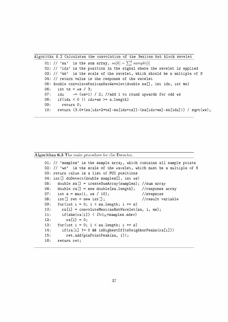
List of Algorithms

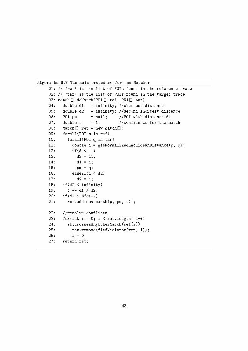
6.1 The main loop for the proposed algorithm . . . . . . . . . . . . . . . . . . 346.2 Calculates the convolution of the Mexican hat block wavelet . . . . . . . . 376.3 The main procedure for the Detector. . . . . . . . . . . . . . . . . . . . . 376.4 The main procedure for the Descriptor . . . . . . . . . . . . . . . . . . . . 396.5 The main procedure for the Super Fast Haar Descriptor . . . . . . . . . . 406.6 The violator function . . . . . . . . . . . . . . . . . . . . . . . . . . . . . . 426.7 The main procedure for the Matcher . . . . . . . . . . . . . . . . . . . . . 436.8 The main procedure for the Warper . . . . . . . . . . . . . . . . . . . . . . 44

8

List of Tables

7.1 Top 5 CPU intensive functions . . . . . . . . . . . . . . . . . . . . . . . . 537.2 Timing results for the various descriptors . . . . . . . . . . . . . . . . . . 557.3 Timing results for the simpli�cation attempts . . . . . . . . . . . . . . . . 577.4 Timing results for the various alignment methods. The time listed for

SW-DPA is the additional time it took to perform the DPA attack . . . . 57

9

List of Abbreviations

AES Advanced Encryption Standard

CPA Correlation Power Analysis

DES Data Encryption Standard

DPA Di�erential Power Analysis

DTW Dynamic Time Warping

EA Elastic Alignment

FT Fourier Transform

MHz Megahertz

POI Point Of Interest

RAM Rapid Alignment Method

RFID Radio Frequency Identi�cation

SIFT Scale Invariant Feature Transform

SNR Signal-to-Noise Ratio

SPA Simple Power Analysis

STFT Short Term Fourier Transform

SURF Speeded Up Robust Features

SW-DPA Sliding Window DPA

U-SURF Upright SURF

XOR Exclusive OR

10

1 Introduction

Nowadays small electronic devices such as smart phones, PDAs and smart cards arebecoming increasingly popular. As a side e�ect of this trend more critical informationis stored in these devices and therefore it is crucial that they are secure. When smartcards entered the consumer market they often had major cryptographic weaknesses inencryption algorithms. Because of the constraints on memory and computing time engi-neers were forced to develop there own encryption methods which were usually not nearlyas well tested as the known encryption algorithms for faster platforms such as personalcomputers. This has changed now, due to more powerful smart cards using proven securealgorithms.A good example that this can back�re has been shown by Garcia et al. [10]. The

MIFARE classic RFID chip was developed by NXP Semiconductors (formerly PhillipsSemiconductors) and is in use for over a decade now. At the moment [10] was publishedNXP claimed that they had sold over 1 billion MIFARE cards and there would be around200 million MIFARE classic cards in use around the world. Due to the fact that the cardhad such a successful history it was marketed as �eld-proven secure. However, at the timethe MIFARE classic chips came to the market there where no RFID readers availablefor consumers. Those few who were able to look at the internals of the chip had tosign a non-disclosure agreement. When eventually researchers were able to evaluate theencryption algorithm used in the chip, they found a major �aw which exposed the keysand thereby allowed full read and write access to the cards. Due to the many applicationsthis discovery had quite some impact and was covered by several media. NXP still sellsMIFARE classic systems but gives a warning when selling, also they no longer claim itis �eld-proven secure.Now the algorithms used in modern chips have become secure, attackers shift focus

to speci�c implementations. One of the new focus areas is the power consumption ofa device. About a decade ago Kocher et al. proposed a method that allowed attackersto extract the secret key used for encryption operations from a small device such as asmartcard [12]. Since then many countermeasures been developed and ways to negate orreduce these countermeasures as well.Kocher's proposed method, DPA (Di�erential Power Analysis), and many variants

depend on the assumption that during the encryption the time intervals between the startof the encryption algorithm and each operation during the encryption remain constantbetween multiple executions of the algorithm (with the same input). Meaning that if ittakes 1 millisecond for the algorithm to get to a certain point in the algorithm, it willtake 1 millisecond to get to that same point every time the algorithm is executed. Instandard algorithms this is usually the case. However by adding bogus operations atrandom points in time or using an unstable clock it is possible to defend against DPA

11

attacks. This thesis proposes a method to negate this countermeasure. By �nding easyto recognize points in the power signal of a device and aligning those points the powersignal is altered so it is susceptible to a DPA attack again.Other algorithms to do this are Static Alignment and Elastic Alignment. Although

Static Alignment can be used for this purpose it does not perform very well. This isdue to the fact that it can only handle di�erences in the starting point of the encryptionalgorithm but not di�erences in the timing of the individual operations. By shiftingthe recorded power signals in such a way that they align around the point of attack itimproves susceptibility to DPA attacks not substantially.Elastic Alignment performs quite well. On the used trace set it was capable of raising

the chance of success from 0% to 95%. It works by aligning samples with each otherthat have the highest correlation. It �rst does this with the minimal resolution of onlytwo samples. It then iteratively increases the resolution of the recorded power signal andaligns again at each step until the full resolution is reached. Although this algorithmperforms well in a lot of cases it has the major drawback that it is slow. Although it hasa computational complexity of O(c ·n) with n being the number of samples, the constantfactor c is quite high. This causes alignment to take several days on large trace sets.The proposed algorithm is designed to deal with the calculation time issues of Elastic

Alignment and it should execute much faster while still producing reasonable results. Itaims to bring down the calculation time from days to hours. The algorithm is inspiredby U-SURF [3] which, given a reference picture, is used to recognize pictures of the samescene/object taking into account di�erences in angle and light. The proposed algorithmuses several techniques used in U-SURF, among most notably the use of block waveletsfor detection and identifying of speci�c points in the recorded power signal. The mainadvantage of block wavelets is that they can be applied inO(1) which makes the algorithmvery fast.The question that this thesis attempts to answer is as follows:

Can we design an alignment algorithm that is fast and yet provides rea-sonable results?

Where 'fast' means that the computation of an typical trace set should complete in hoursas opposed to Elastic Alignment were it takes days. With 'reasonable' is meant that theresulting aligned traces should be usable to perform a DPA-style attack. To answer thequestion ideas from the SIFT and U-SURF algorithms are used and adapted to �t thisapplication.We translate the ideas of SIFT and U-SURF from the 2 dimensions (images) to one

dimension (power traces). Our one dimensional version needs to be a lot more robustagainst noise since power traces contain a lot more noise than the images used for objectrecognition. Finally we add a step to the algorithm that takes care of the actual alignmentof the traces.This thesis is organized as follows. Chapter 2 describes the basics of side channel

attacks such as DPA and several countermeasures. Chapter 3 covers the algorithms cur-rently available, Sliding Window DPA, Static Alignment and Elastic Alignment. Chapter

12

4 gives some background about signal processing and substantiate the choice for the useof wavelets for this application. Chapter 5 covers the fundamentals of SIFT and U-SURFon which the proposed algorithm is based. The proposed algorithm is described into de-tail in Chapter 6 and Chapter 7 discusses the setup for our experiments. Last but notleast, in Chapter 8 the conclusion and further research is covered.

13

2 CPA and Alignment

2.1 Power Analysis

Attacking an electronic device by analyzing the algorithm mathematically is consideredattacking over the main channel. One tries to �nd a mathematical or logical �aw inthe algorithm (or protocol) and tries to exploit that. If this succeeds, every device thatimplements the same algorithm is vulnerable to the same attack. There are other attackssmart cards and small electronic devices have weaknesses against. Every computer chipemits heat, sound and light during a calculation. Also the electromagnetic �eld andthe power consumption change during a calculation. Side channel analysis makes use ofthe information that is exposed through these side products of the computation. Thedata that is measured from such a side channel can be combined with a model thatgives the relation of the side channel leakage and the internal activity of the chip. Withan accurate enough model and an unprotected device it is possible to �nd out what thedevice is computing. With side channel analysis the focus is not so much on the algorithmitself but more on a speci�c implementation. If one succeeds in breaking the securityof a device through side channel analysis it does not mean that every other device thatuses the same algorithm is also vulnerable to this same attack. Di�erent chips can havedi�erent implementations of the same algorithm and can have di�erent countermeasuresto prevent side analysis. The type of side channel attack that inspired this thesis is calledpower analysis, which was invented by Kocher et al. a decade ago [12]. Power analysisfocuses on the power usage of a device and tries to map this to the internal calculations.One of the most notable power analysis attacks is called Di�erential Power Analysis.

This works roughly as follows.

1. First the timing of the leakage is determined. This should be a position in thealgorithm where some bits of the key k are combined with a known non-constantvalue v. This is normally a piece of the plaintext when attacking the beginning ofthe encryption algorithm or a piece of the cyphertext when attacking at the end.We denote the piece of the key and the known value combined as f(v, k).

2. Now we feed the device a large number of random plaintexts and let it encryptthese. How many are necessary depends on the countermeasures present in thedevice and the amount of power leakage and measurement noise. In practice thenumber of plaintexts needed varies from thousands to millions.

3. For each of the possible values of k the bit f(v, k) is predicted. It is importantthat the number of possible values of k is limited. For every possible value of kthe trace set is split into two groups. One, where the predicted bit f(v, k) is 0

14

and the other where the bit is 1. If the guess for k was correct the majority oftraces in each group group are traces where the actual bit matches the predictedbit f(v, k) . If the guess for k was incorrect the traces are split randomly and thetwo groups contain traces more or less 50% of traces where the actual bit matchesthe predicted bit and 50% of the traces where the actual bit does not match thepredicted bit.

4. The traces from each group are averaged. Both the averaged traces are subtractedfrom each other. Since the traces were split on the basis of the predicted valueof f(v, k) all sample points not representing this bit average to more or less thesame value in both of the groups. Subtracting those results in a value near 0. Thesame happens for the sample point where f(v, k) is processed if k was wrong. Ifk was right this sample point averages to power consumption value that is neededto process the value of the predicted bit for each group. Subtracting these twoaverages does not yield a value near 0. So ideally the result of these four steps is atrace where every sample point is 0 and a clear peak (positive or negative) at theposition where f(v, k) was processed.

The above process is repeated for every key bit. The statistical test used to determinethe relationship between the hypothetical power consumption and the measured powerconsumption is called a side channel distinguisher. A popular variant of DPA is Corre-lation Power Analysis (CPA)[5]. CPA does not use the di�erence in means as the sidechannel distinguisher but uses Pearson correlation. It takes longer to compute but itis more sensitive for the linear dependencies of power in data and thus provides betterresults in general.Simple Power Analysis (SPA) [12] requires the attacker to analyze the power signal

manually by �nding patterns in the signal. This is, despite the name, far from simpleand requires quite some experience on the attacker side. However, typically only a fewtraces are needed to perform SPA. Therefore it might be the only option to go with whennot many traces are available.Since the DPA and CPA rely on respectively averaging and correlating traces, it is

important that the traces are aligned in the time domain. A speci�c calculation stepof the chip-under-attack should occur at the same position in the time domain for allthe measured traces. If this is not the case, combining the traces averages out themeasurements and lose the information stored in there. Some of the countermeasuresagainst DPA-style attacks are based on this principle and aim to create variances in thetime domain.

2.2 Countermeasures

There is a strong push from certi�cation bodies such as Common Criteria and EMVcoon manufacturers to keep up with the latest techniques, while balancing these with theireconomical constraints. They therefore implement a range of countermeasures to reducethe possibilities of DPA-style attacks. The main goal of the countermeasures against

15

DPA or CPA is to minimize or hide the dependencies between the power consumptionand the intermediate values of the encryption algorithm used. Several countermeasureshave already been developed and successfully put in use against DPA or CPA attacks.Although this research is focused on one speci�c way to counter one speci�c class ofcountermeasures (time domain hiding, including random delays and unstable clocks) itis important to know that this is only one of the few types of countermeasures. Mostcountermeasures fall in one of two categories which are explained in the remainder ofthis section.

2.2.1 Masking

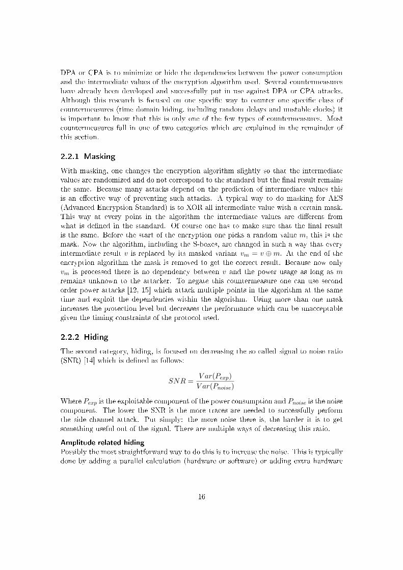
With masking, one changes the encryption algorithm slightly so that the intermediatevalues are randomized and do not correspond to the standard but the �nal result remainsthe same. Because many attacks depend on the prediction of intermediate values thisis an e�ective way of preventing such attacks. A typical way to do masking for AES(Advanced Encryption Standard) is to XOR all intermediate value with a certain mask.This way at every point in the algorithm the intermediate values are di�erent fromwhat is de�ned in the standard. Of course one has to make sure that the �nal resultis the same. Before the start of the encryption one picks a random value m, this is themask. Now the algorithm, including the S-boxes, are changed in such a way that everyintermediate result v is replaced by its masked variant vm = v ⊕m. At the end of theencryption algorithm the mask is removed to get the correct result. Because now onlyvm is processed there is no dependency between v and the power usage as long as mremains unknown to the attacker. To negate this countermeasure one can use secondorder power attacks [12, 15] which attack multiple points in the algorithm at the sametime and exploit the dependencies within the algorithm. Using more than one maskincreases the protection level but decreases the performance which can be unacceptablegiven the timing constraints of the protocol used.

2.2.2 Hiding

The second category, hiding, is focused on decreasing the so-called signal-to-noise ratio(SNR) [14] which is de�ned as follows:

SNR =V ar(Pexp)

V ar(Pnoise)

Where Pexp is the exploitable component of the power consumption and Pnoise is the noisecomponent. The lower the SNR is the more traces are needed to successfully performthe side channel attack. Put simply: the more noise there is, the harder it is to getsomething useful out of the signal. There are multiple ways of decreasing this ratio.

Amplitude related hiding

Possibly the most straightforward way to do this is to increase the noise. This is typicallydone by adding a parallel calculation (hardware or software) or adding extra hardware

16

components that generate random noise. This principle shows one of the advantages ofa hardware implementation opposed to a software implementation. In hardware imple-mentations, where the algorithm is implemented by linking logical gates, the algorithmsare executed much faster and often there exists some parallelism which introduces noiseas opposed to software implementations where a general purpose processor needs to ex-ecute assembler code. When parts of the algorithm are executed in parallel the powersignal does not map to a single point in the computation anymore. Now the power signalconsists of the sum of multiple computations. This makes DPA-style attacks much moredi�cult and increases the number of traces needed considerably.One can of course also reduce the usable signal. By ensuring that every operation uses

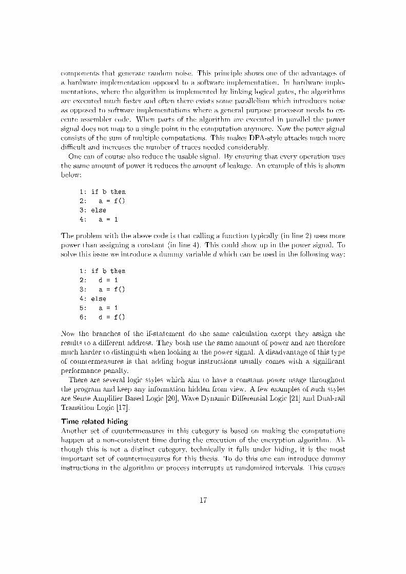
the same amount of power it reduces the amount of leakage. An example of this is shownbelow:

1: if b then

2: a = f()

3: else

4: a = 1

The problem with the above code is that calling a function typically (in line 2) uses morepower than assigning a constant (in line 4). This could show up in the power signal. Tosolve this issue we introduce a dummy variable d which can be used in the following way:

1: if b then

2: d = 1

3: a = f()

4: else

5: a = 1

6: d = f()

Now the branches of the if-statement do the same calculation except they assign theresults to a di�erent address. They both use the same amount of power and are thereforemuch harder to distinguish when looking at the power signal. A disadvantage of this typeof countermeasures is that adding bogus instructions usually comes with a signi�cantperformance penalty.There are several logic styles which aim to have a constant power usage throughout

the program and keep any information hidden from view. A few examples of such stylesare Sense Ampli�er Based Logic [20], Wave Dynamic Di�erential Logic [21] and Dual-railTransition Logic [17].

Time related hiding

Another set of countermeasures in this category is based on making the computationshappen at a non-consistent time during the execution of the encryption algorithm. Al-though this is not a distinct category, technically it falls under hiding, it is the mostimportant set of countermeasures for this thesis. To do this one can introduce dummyinstructions in the algorithm or process interrupts at randomized intervals. This causes

17

changes in the time dimension. Both DPA and CPA combine traces to enhance therelation between the power trace and the computation in the device. When this counter-measure is applied it becomes much harder to perform the attack successfully. Note thatit is still possible to perform the attack but the number of traces needed increases withseveral orders of magnitude to average out the e�ects of the shifted time dimension. Adisadvantage is that there is a performance penalty due to the fact that the algorithmcontains dummy instructions and that the values for the randomized intervals need tobe computed.Changes in the time dimension can also be achieved by using an unstable clock. This

causes operations to have a non-constant time, even if they are the same [14].This thesis focuses on this last type of countermeasures. By aligning the traces we

reduce the changes in the time dimension so fewer traces are needed to successfullyattack the implementation. This is particular interesting due to the fact that moderncards usually have an unstable clock, added noise and added dummy instructions ascountermeasures.

18

3 Dealing with time shifted traces

3.1 Sliding window DPA

This method was proposed by Clavier et al. in 2000 [7]. Sliding window DPA (or SW-DPA) is speci�cally designed to counter random process interrupts (RPI). When RPI areused as a countermeasure the position of the leakage that is exploited by DPA can shifta few clock cycles. SW-DPA is based on this assumption, Clavier et al. describes it asfollows.

�Suppose the spike on the di�erential trace should be seen after n cycles. IfRPIs occurred, a spike appears after n + Cn cycles, where the delay Cn =∑n

i=1 ci, ci being the i-th cycle, with ci = 1 if an RPI occurred and ci = 0 ifnot.�[7]

When traces are averaged during the DPA the resulting spike follows a Gaussian dis-tribution. The top of this distribution is usually to low to be useful in a DPA attack.Clavier et al. proposes to reconstruct this spike by averaging consecutive clock cycles.This way, when looking at multiple traces, the spike information that was spread overseveral clock cycles is now combined and put back in one place.In practice this means that each clock cycle in a power trace is replaced by the average

of itself and a number of previous clock cycles. The two main parameters of this methodare the number of cycles to average (the window size) and the number of samples perone clock cycle. The correct number of cycles to average depends on how many RPIhave occurred before the spike. If the number is way o�, the samples that contain spikeinformation are averaged with other samples reducing the height of the spike again. Thereis no way of exactly knowing how many RPI occur on average before the spike so severalvalues have to be tried. The number of samples per clock cycle depends on the settingsduring acquisition of the power traces. This is known by the attacker.In [22] it was shown that SW-DPA performs fairly well. However when an unstable

clock is used the performance drops drastically. This is not surprising since the algorithmassumes a stable clock of which the frequency is set in parameters of the algorithm.

3.2 Static Alignment

This algorithm is proposed by Mangard et al. in 2007 [14]. The basic idea is as follows:the attacker selects an fragment in the reference trace close to the area where the attacktakes place. Then the algorithm aims to �nd this same fragment in the other traces andshifts the other trace so that the reference fragments are aligned. The attacker should pick

19

Figure 3.2.1: Static Alignment example. The two unaligned traces have the fragmentsselected that will be used for Static Align

a fragment with a unique pattern, since it reduces confusion of the algorithm. Althoughthis does not fully counter an unstable clock or random delays it often does reduce thenumber of traces needed to successfully perform a DPA attack. This is due to the factthat aligning at a certain point in a trace reduces the noise and thereby increases theSNR around that point.The Static Alignment implementation used for this thesis uses normalized cross-correlation

to identify the fragment where the traces should be aligned. The fragment with the high-est cross-correlation with the reference fragment is selected as the point where to align.Usually this fragment can be found near the position where the reference is found in thereference trace to use this as heuristic the attacker can specify a maximum shift so thealgorithm only has to search within that window. If the best cross-correlation found isbelow a threshold set by the attacker the entire trace is excluded from the result. In�gure 3.2.1 two traces can be seen. Trace 0 is the reference trace here where the attackerselects a fragment for the algorithm to align on. Trace 1 is the only target trace here,the selection here shows the same fragment as in the reference trace.

3.3 Elastic Alignment

Elastic Alignment by van Woudenberg et al. in 2011 [22] is conceptually more di�cultthan Static Alignment. It aims to stretch and shrink the trace in such a way that thetime dimension is fully restored and the unstable clock and/or random delays are fullynegated. It does this by calculating the distance (absolute di�erence) between everysample of the target trace with every sample in the target trace. This results in a matrixT of size N · N . The goal is to �nd a path from the lower left corner (the start ofboth traces) to the upper right corner (the end of both traces). This path is called thewarppath, it is used to warp the target trace so is aligned with the reference trace. Usingdynamic programming techniques the path is selected where the sum of all the distancesis the lowest. The cells in the matrix that are selected represent which sample points of

20

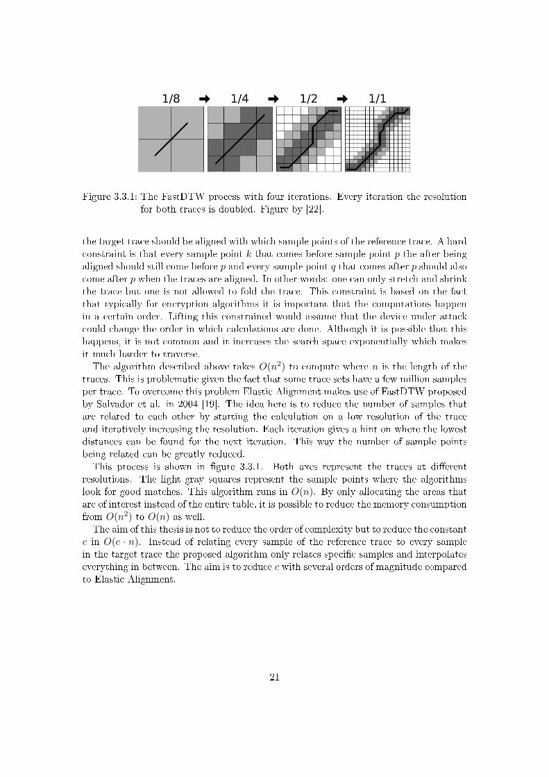
Figure 3.3.1: The FastDTW process with four iterations. Every iteration the resolutionfor both traces is doubled. Figure by [22].

the target trace should be aligned with which sample points of the reference trace. A hardconstraint is that every sample point k that comes before sample point p the after beingaligned should still come before p and every sample point q that comes after p should alsocome after p when the traces are aligned. In other words: one can only stretch and shrinkthe trace but one is not allowed to fold the trace. This constraint is based on the factthat typically for encryption algorithms it is important that the computations happenin a certain order. Lifting this constrained would assume that the device under attackcould change the order in which calculations are done. Although it is possible that thishappens, it is not common and it increases the search space exponentially which makesit much harder to traverse.The algorithm described above takes O(n2) to compute where n is the length of the

traces. This is problematic given the fact that some trace sets have a few million samplesper trace. To overcome this problem Elastic Alignment makes use of FastDTW proposedby Salvador et al. in 2004 [19]. The idea here is to reduce the number of samples thatare related to each other by starting the calculation on a low resolution of the traceand iteratively increasing the resolution. Each iteration gives a hint on where the lowestdistances can be found for the next iteration. This way the number of sample pointsbeing related can be greatly reduced.This process is shown in �gure 3.3.1. Both axes represent the traces at di�erent

resolutions. The light gray squares represent the sample points where the algorithmslook for good matches. This algorithm runs in O(n). By only allocating the areas thatare of interest instead of the entire table, it is possible to reduce the memory consumptionfrom O(n2) to O(n) as well.The aim of this thesis is not to reduce the order of complexity but to reduce the constant

c in O(c · n). Instead of relating every sample of the reference trace to every samplein the target trace the proposed algorithm only relates speci�c samples and interpolateseverything in between. The aim is to reduce c with several orders of magnitude comparedto Elastic Alignment.

21

4 Alignment with wavelets

The proposed algorithm does the same as Elastic Alignment but in a di�erent way. Theaim is to create an algorithm that is signi�cantly faster than Elastic Alignment. Despitethe linear complexity of Elastic Alignment, it can still take several days to align a typicaltrace set for modern cards. The proposed algorithm aims to reduce the running timewith several orders of magnitude. Although the aligned trace quality is very important(the better the quality the less traces are needed), sacri�cing some quality in exchangefor speed is acceptable.The proposed algorithm tries to �nd points of interest (POI) in the reference trace

and then tries to �nd the same points of interest in the target trace. Matching pointsare used for the alignment. A point of interest can be a peak or a slope or anything elsethat is fast to detect and can be detected repeatedly in other traces from the same set.To match the POIs from the reference trace and the target trace for each POI a featurevector is generated based on the samples around the POI. This is feature vector is calledthe description of the POI. The algorithm aims for a unique description per POI so therewon't be any confusion when matching the POIs.There are many ways to detect POIs and create a description of their context. A good

detection algorithm is fast, robust to noise and �nds the same POIs in the reference traceand in the target trace. A good description algorithm is fast and creates a descriptionthat is unique for every POI in a trace but is the same for the same POI in the referenceand in the target trace. For both these tasks we choose to use wavelets because they arevery fast and perform well when it comes to catching the characteristics of a signal. Inthe remainder of we explain why wavelets are preferred over the more traditional way ofanalyzing a signal by using a Fourier Transform.

4.1 Fourier Transform

In the 19th century Fourier showed that any periodic function can be expressed as anin�nite sum of periodic complex exponential functions [9]. In other words any periodicfunction can be expressed through much simpler functions. This idea was later gener-alized to non-periodic functions and discretised so it was suitable for fast computation.Even up to now this has been arguably the most popular tool to analyze signals. In thissubsection we explain brie�y what it does and what the disadvantages are in the contextof this thesis.A Fourier transform (FT) gives us an idea of what frequencies appear in the signal

and with what strength. This can be illustrated by the example shown in �gure 4.1.1.Figure 4.1.1 shows a periodic signal and the Fourier transform of that signal.

22

0 0.05 0.1 0.15 0.2 0.25 0.3 0.35 0.4 0.45 0.5−3

−2

−1

0

1

2

3

4

Time (s)

Am

plitu

de

0 50 100 150 200 2500

10

20

30

40

50

60

Frequency (Hz)

Pow

er

Fourier transform on the stationary signal

Figure 4.1.1: A stationary signal (left) consisting out of a 10Hz, 25Hz, 50Hz and a 100Hzwave and its Fourier transform (right).

0 0.2 0.4 0.6 0.8 1−1

−0.8

−0.6

−0.4

−0.2

0

0.2

0.4

0.6

0.8

1

Time (s)

Am

plitu

de

0 50 100 150 200 2500

2

4

6

8

10

12

14

16

18

Frequency (Hz)

Pow

erFourier transform on the non−stationary signal

Figure 4.1.2: A non-stationary signal(left) consisting out of a 10Hz, 25Hz, 50Hz and a100Hz wave and its Fourier transform (right).

In the Fourier transform we see four peaks, one peak at each of the frequencies theoriginal signal consisted of. The peaks should be the same height but because the FTwas computed here on a sample set instead of the actual function some peaks are higherthan others. The peak heights vary depending on the size of the sample set and on thesample frequency. Nonetheless, the Fourier plot gives us a very clear description aboutthe signal. Whereas the original signal seems somewhat chaotic to an inexperienced eye,the Fourier transform can easily be read by anyone.Now a slightly di�erent signal, it contains the same frequencies as before (10Hz, 25Hz,

50Hz and 100Hz) but instead of all the frequencies at the same time (as it was in theprevious example), here the frequencies are consecutive so there exists only one frequencyat a time. The resulting plot is shown in �gure 4.1.2.In the same �gure we see that although the original signal was quite di�erent from

23

the periodic signal, the FT looks very similar. In the FT we see four peaks again, onefor each frequency. We also see some noise here, this is because of the transitions fromone frequency to another. Note that for real signals noise is very common and cannot beused to identify or describe signals. Except for the noise the FT looks the same as for the�rst example. The amplitudes of the Fourier transformed signals are indistinguishable.This is because an implicit assumption of FT. It assumes that the signal contains the

same frequencies during the entire signal (from minus in�nity to in�nity). These typesof signals are called stationary signals. The second example however, is a non-stationarysignal as its frequencies change over time. Most signals that appear in real life are non-stationary. The power traces we want to analyze are never stationary since they arebased on the computations in a computer chip. So Fourier transforms are not the bestoption for analyzing them.Note that depending on the implementation an FT transform can also give information

about the phase of a frequency (whether it is shifted to the left or the right). Although thisinformation does help at di�erentiating the examples used here, one can easily constructan example (by shifting the frequencies slightly until they match in both the stationaryand the non-stationary example) where an FT would fail to di�erentiate the signals again.For simplicity's sake we ignore the phase information here as it does not fully counterthe arguments presented here.

4.2 Short Term Fourier Transform

To be able to deal with non-stationary signals Short Term Fourier Transform (STFT)was designed [1]. This is basically the same as FT but uses a window. Instead oftransforming the entire signal STFT only transforms the signal within the window. Thewindow has a prede�ned width and starts at the beginning of the signal. After eachtransform the window shifts over the signal until it reaches the end performing an FT atevery step. This gives us information about the frequency domain and about the timedomain of the signal. Figure 4.2.1 shows the results of the STFT on the two examplesused earlier in this section.Now we can clearly distinguish the signals. However, a signi�cant problem with STFT

is the width of the window. A large window gives us poor time-resolution (the larger thewindow the more it STFT looks like a normal FT). On the other hand if the window issmall it has less resolution for frequencies. In the case of a small window the peaks ofthe FT widen so it becomes less clear what the actual frequency was.The appropriate window size for STFT is application dependent. If the frequency

components are well separated one can sacri�ce some frequency resolution to get a bettertime resolution and vice versa. The window size comes down to a choice between the agood resolution in the frequency dimension and the time dimension.Note that this problem is inherent to a physical phenomenon and is known as the

Heisenberg Uncertainty Principle. Published by W. Heisenberg in 1927 this principlestates that is not possible to measure certain pairs of physical properties simultaneouslywith arbitrary precision. The more precisely one property is measured the less precisely

24

Figure 4.2.1: The results of the STFT on the stationary (left) and the non-stationary(right) signal

the other can be measured. A common example of such a pair is position and momentumof a particle. Here the frequency and the position of a wave are such a pair. It basicallymeans that one cannot know what spectral components exist at what instances of time.One can only know the time intervals in which certain bands of frequencies exist. This isa trade-of which appears very clearly when using STFT. According Heisenberg's principleit is impossible to solve window problem of STFT perfectly, however one can make choicethat works well based on the application.

4.3 Wavelet Transform

Another technique that tries to deal with the ine�ectiveness in certain applications ofFT is wavelet transform. The term 'wavelet' used in digital signal processing dates backseveral decades [18] and means 'small wave'. A wavelet can be visualized as a briefoscillation1. It is a non-stationary signal with an amplitude that starts out at zero,increases, and then decreases back to zero. A few examples of wavelets are shown in�gure 4.3.1.By calculating the convolution of a wavelet at a sample in the signal one gets a response

that tells how well the wavelet matches the signal at that point. If this is done for everysample in the signal the series responses shows where and how well the signal matches thewavelet. Often the wavelet is applied multiple times with di�erent scales. By doing thisit is possible to describe a signal at low frequencies (large wavelets) and high frequencies(small wavelets). A wavelet can be scaled with the following formula:

ψa,b(t) =1√aψ(t− ba

)

1The source of this quote is unknown

25

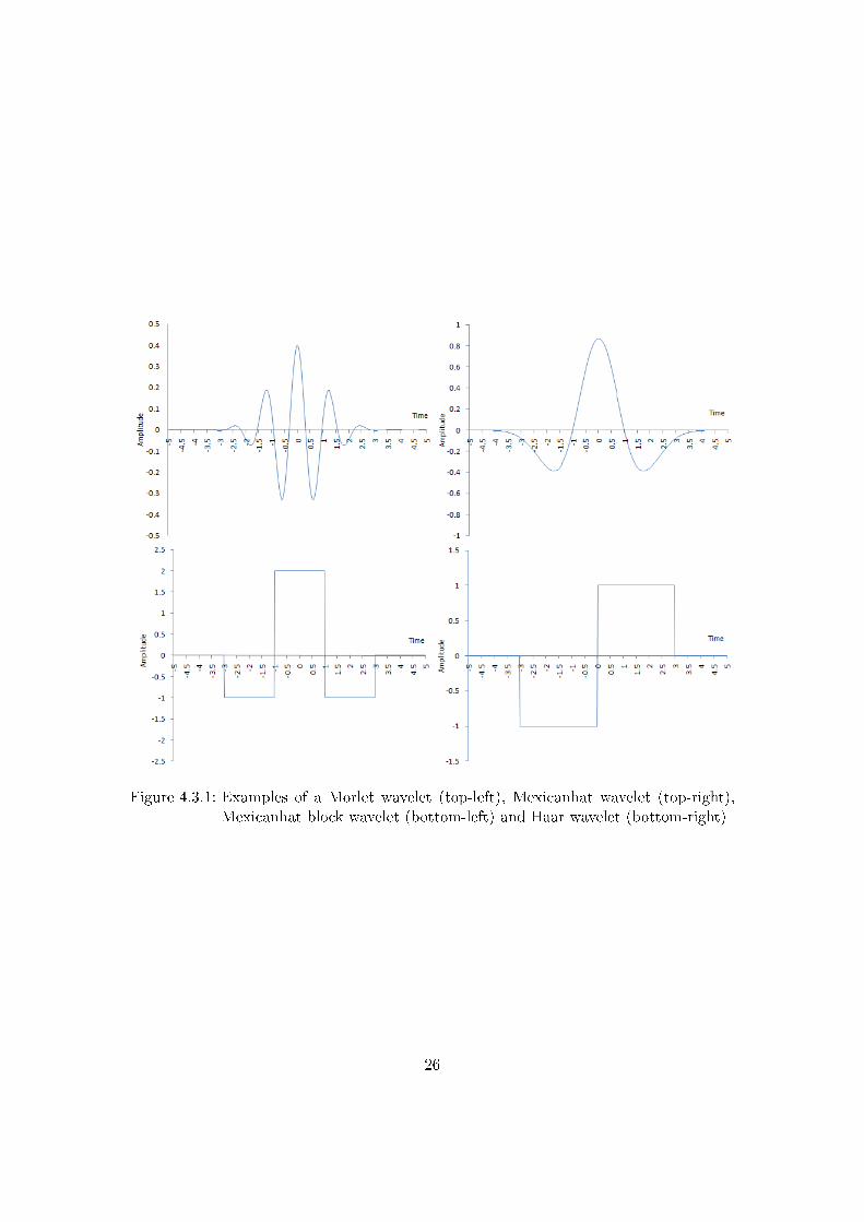
Figure 4.3.1: Examples of a Morlet wavelet (top-left), Mexicanhat wavelet (top-right),Mexicanhat block wavelet (bottom-left) and Haar wavelet (bottom-right)

26

Figure 4.3.2: The response of 4 wavelets on the non-stationary signal

Where ψ is the wavelet function with (positive) scale a at o�set b. A wavelet transformcan mathematically be expressed in the following way:

WTψ{x}(a, b) =ˆx(t)ψa,b(t)dt

Where ψa,b is the scaled wavelet function and x(t) is here the signal over time t. Thissimply means that you �rst stretch the wavelet by using a and place it on the signal thatyou want to analyze at b. Then pass over the samples of the signal and multiply everysample with the value of the wavelet at that position. Because most values of ψ are zeroonly the part of the signal around the center of the wavelet give nonzero values. Thesum of those values is called the response for the wavelet at position b. Calculating thisfor every possible (or useful) b results in a wavelet transform at scale a. By doing thisfor several values of a we get a 2 dimensional matrix with wavelet responses. The resultof a wavelet transform on the consecutive frequencies example from �gure 4.1.2 is shownin �gure 4.3.2.Figure 4.3.2 shows at what time which wavelet responses are the highest in the signal.

The four graphs show a clear distinction for every frequency. Note that the choice of thewavelet matters, here the Mexicanhat wavelet is used with 4 di�erent scales. Dependingon what patterns need to be found di�erent wavelets can be used. For example whensearching for a speci�c frequency one could use a sine (or cosine) with that frequency. Toturn this into a wavelet the sine is multiplied with a Gaussian distribution curve de�nedby the following formula:

Gaussσ,µ(x) =1√2πσ2

· e−(x−µ)2

2σ2

27

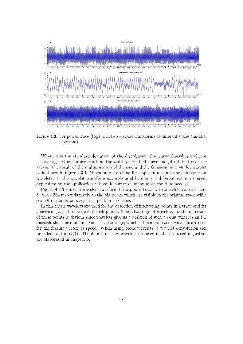
Figure 4.3.3: A power trace (top) with two wavelet transforms at di�erent scales (middle,bottom)

Where σ is the standard deviation of the distribution this curve describes and µ isthe average. One can use σto tune the width of the bell curve and µto shift it over thex-axis. The result of the multiplication of the sine and the Gaussian is a Morlet waveletas is shown in �gure 4.3.1. When only searching for slopes in a signal one can use Haarwavelets. In the wavelet transform example used here only 4 di�erent scales are used,depending on the application this could su�ce or many more could be needed.Figure 4.3.3 shows a wavelet transform for a power trace with wavelet scale 384 and

6. Scale 384 responds nicely to the big peaks which are visible in the original trace whilescale 6 responds to every little peak in the trace.In this thesis wavelets are used for the detection of interesting points in a trace and for

generating a feature vector of such points. The advantage of wavelets for the detectionof these points is obvious since wavelets give us a position of such a point whereas an FTdiscards the time domain. Another advantage, which is the main reason wavelets are usedfor the feature vector, is speed. When using block wavelets, a wavelet convolution canbe calculated in O(1). The details on how wavelets are used in the proposed algorithmare elaborated in chapter 6.

28

5 SIFT and U-SURF

The proposed algorithm is inspired by SIFT and U-SURF. The purpose of these algo-rithms is object recognition in images. However the techniques used in these algorithmscan be translated into recognizing speci�c points in a power trace. The proposed �ndspoints in two traces and aligns these points. The di�erence is that here we only work in1 dimension (which reduces computational complexity) but we have to deal with a lotmore noise (which can confuse the algorithm). The remainder of this section describesthe original SIFT and U-SURF algorithm.

5.1 SIFT

SIFT stands for Scale Invariant Feature Transform. It is a feature generation methodproposed by Lowe in 1999 [13]. The features generated are used to recognize objectsin images. Object recognition algorithms have to be robust against scaling, translation,rotation and noise in the images. SIFT aims to achieve a certain robustness by using amultiple �lter approach. The algorithm has three phases.

Detection phase

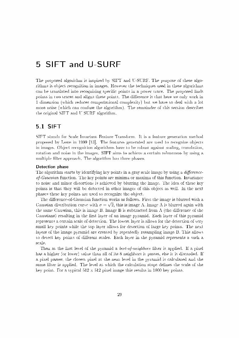
The algorithm starts by identifying key points in a gray scale image by using a di�erence-of-Gaussian function. The key points are minima or maxima of this function. Invarianceto noise and minor distortions is achieved by blurring the image. The idea of these keypoints is that they will be detected in other images of this object as well. In the nextphases these key points are used to recognize the object.The di�erence-of-Gaussian function works as follows. First the image is blurred with a

Gaussian distribution curve with σ =√2, this is image A. Image A is blurred again with

the same Gaussian, this is image B. Image B is subtracted from A (the di�erence of theGaussians) resulting in the �rst layer of an image pyramid. Each layer of this pyramidrepresents a certain scale of detection. The lowest layer is allows for the detection of verysmall key points while the top layer allows for detection of large key points. The nextlayers of the image pyramid are created by repeatedly resampling image B. This allowsto detect key points of di�erent scales. Each layer in the pyramid represents a such ascale.Then at the �rst level of the pyramid a best-of-neighbors �lter is applied. If a pixel

has a higher (or lower) value than all of its 8 neighbors it passes, else it is discarded. Ifa pixel passes, the closest pixel at the next level in the pyramid is calculated and thesame �lter is applied. The level at which the calculation stops de�nes the scale of thekey point. For a typical 512 x 512 pixel image this results in 1000 key points.

29

For each pixel Aij in image A the gradient magnitude, Mij , and the orientation, Rij ,are calculated using pixel di�erences:

Mij =√(Aij −Ai+1,j)2 + (Aij −Ai,j+1)2

Rij = atan2(Aij −Ai+1,j , Ai,j+1 −Ai,j)

Where the atan2(x, y) function is a variation on the standard arctan(x) function.The atan2 function is common in programming languages (C, C++, Java, .NET...) forcalculating an angle between the x-axis and a point given the coordinates x and y. It isde�ned as follows:

atan2(x, y) =

arctan( yx) x > 0

π + arctan( yx) y ≥ 0, x < 0

−π + arctan( yx) y < 0, x < 0π2 y > 0, x = 0

−π2 y < 0, x = 0

unde�ned y = 0, x = 0

Since SIFT aims to be robust against rotation the orientation of each key point isimportant. For each key point a canonical orientation is selected by �nding a peak in ahistogram. The histogram consists of 36 bins covering the 360 degrees of orientation. Forevery pixel around a key point with coordinates (i, j),Mij is weighted against a Gaussian(σ = 3 ·scale, where scale is the scale of the key point) window and then accumulated inthe bin corresponding with Rij . The histogram is smoothed and then the peak is selectedwhich de�nes the orientation of the speci�c key point.

Description Phase

The SIFT algorithm then calculates some features which bare some similarities to theinferior temporal cortex in primate vision. The area around each key point is downsam-pled to a 4 x 4 area and is represented with 8 orientation planes. The planes are smallgradient matrices that each represent 45 degrees of the 360 degrees of orientation. Onlythe gradients (Mij) from the pixels that have the an orientation (Rij)that is representedby the speci�c plane are copied to the plane. The rest of the values in the plane are�lled using linear interpolation. The orientation planes are blurred to allow for shifts inpositions of the gradients. These planes are the feature set for the speci�c key point.

Matching Phase

SIFT now looks for key point matches in the object-to-be-found-image and the search-image. If enough key points from the object-to-recognize match in the image where theobject needs to be found. By using a variant of the kd-tree structure (k-dimensional tree,a data structure that, given an element, allows for fast retrieval of its nearest neighbors)called the best-bin-�rst search algorithm proposed by Beis et al. [4], SIFT is able toquickly look up and compare key points. The best-bin-�rst algorithm is a approximation

30

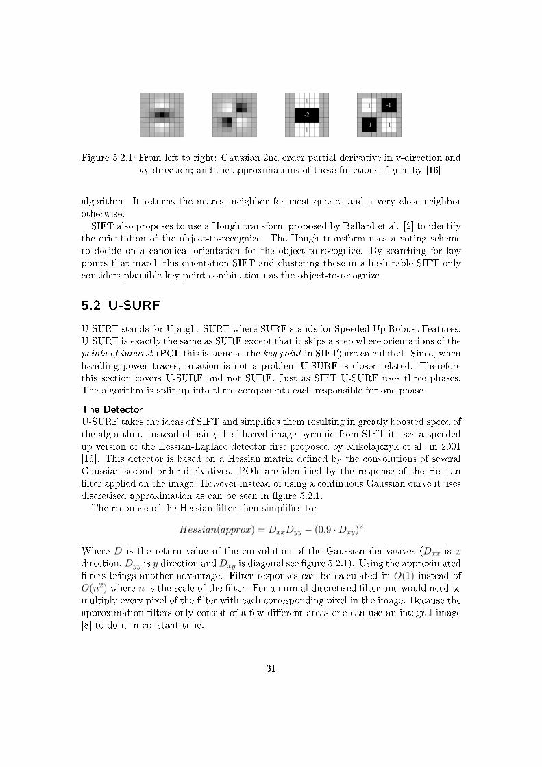
Figure 5.2.1: From left to right: Gaussian 2nd order partial derivative in y-direction andxy-direction; and the approximations of these functions; �gure by [16]

algorithm. It returns the nearest neighbor for most queries and a very close neighborotherwise.SIFT also proposes to use a Hough transform proposed by Ballard et al. [2] to identify

the orientation of the object-to-recognize. The Hough transform uses a voting schemeto decide on a canonical orientation for the object-to-recognize. By searching for keypoints that match this orientation SIFT and clustering these in a hash table SIFT onlyconsiders plausible key point combinations as the object-to-recognize.

5.2 U-SURF

U-SURF stands for Upright-SURF where SURF stands for Speeded Up Robust Features.U-SURF is exactly the same as SURF except that it skips a step where orientations of thepoints of interest (POI, this is same as the key point in SIFT) are calculated. Since, whenhandling power traces, rotation is not a problem U-SURF is closer related. Thereforethis section covers U-SURF and not SURF. Just as SIFT U-SURF uses three phases.The algorithm is split up into three components each responsible for one phase.

The Detector

U-SURF takes the ideas of SIFT and simpli�es them resulting in greatly boosted speed ofthe algorithm. Instead of using the blurred image pyramid from SIFT it uses a speededup version of the Hessian-Laplace detector �rst proposed by Mikolajczyk et al. in 2001[16]. This detector is based on a Hessian matrix de�ned by the convolutions of severalGaussian second order derivatives. POIs are identi�ed by the response of the Hessian�lter applied on the image. However instead of using a continuous Gaussian curve it usesdiscretised approximation as can be seen in �gure 5.2.1.The response of the Hessian �lter then simpli�es to:

Hessian(approx) = DxxDyy − (0.9 ·Dxy)2

Where D is the return value of the convolution of the Gaussian derivatives (Dxx is xdirection, Dyy is y direction andDxy is diagonal see �gure 5.2.1). Using the approximated�lters brings another advantage. Filter responses can be calculated in O(1) instead ofO(n2) where n is the scale of the �lter. For a normal discretised �lter one would need tomultiply every pixel of the �lter with each corresponding pixel in the image. Because theapproximation �lters only consist of a few di�erent areas one can use an integral image[8] to do it in constant time.

31

An integral image works as follows. Every pixel in the the integral image, Ixy, is thesum of all the pixels to the left and above of this pixel in the original image, ixy. Thevalue of each pixel in the integral image is de�ned as follows:

Ixy = ixy + Ix−1,y + Ix,y−1 − Ix−1,y−1

Now the sum of an area in the original image can easily be calculated:∑A<x′≤B;C<y′≤D

ix′,y′ = IA,C + IB,D − IB,C − IA,D

One can do the convolution of a box area in the �lter by multiplying value of that area,as is shown in 5.2.1, with the sum of the corresponding area in the original image. Thistakes constant time regardless of the size of the �lter. The Hessian �lter is applied atdi�erent scales, just like SIFT a best-of-neighbor �lter is applied. The resulting pixelsare the POIs.

The Descriptor

For the generation of the features Haar wavelets are used. They consist of box areasas well and are therefore also fast with the use of the integral image. A window of 20times the scale of the POI is split up into smaller 4 x 4 subregions. For every pixelin a subregion a Haar wavelet response in y-direction, dy, and in x-direction, dx, arecalculated. These responses are weighted with a Gaussian (σ = 3.3 · scale) centered atthe POI. Then per subregion all the responses dx and dy are summed and form the �rstset of features for the subregion. The responses |dx| and |dy| are also summed and formthe second set. At four features per subregion and 16 subregions each POI is describeby 64 features.

The Matcher

The matching works the same as with SIFT. It also uses the best-bin-�rst search algorithmproposed by Beis et al. [4] and Hough transforms proposed by Ballard et al. [2] to de�nea canonical orientation for the object-to-detect. In addition to this U-SURF adds anadditional indexing step based on the sign of the Hessian response.

32

6 The Algorithm

6.1 Outline

Our proposed algorithm tries to reduce the e�ects of an unstable clock and dummyoperations by aligning all traces in a set to a reference trace. This is a common approachwhich is also used by Static Alignment and Elastic Alignment. The reference trace canbe the result of a calculation (such as averaging several traces) or just be one trace ofthe set. For simplicity's sake in this thesis we use the �rst trace in the set. In this thesiswe refer to the trace we align to as the reference trace and the traces that need to bealigned as the target traces.In order to limit the amount of tunable settings for attackers every parameter in the

algorithm was related to properties of the trace. This way the constants used in thealgorithm are not speci�c for one trace set causing the algorithm to be easier to use.The algorithm discussed in this thesis is based on the ideas used in the SIFT [13]

algorithm and variants on that. To be more speci�c the proposed algorithm is inspiredby U-SURF [3]. It consists out of four components. First the Detector �nds pointsof interest (POI) in the reference trace and the target traces. The Descriptor thendescribes the POIs based on their context. These descriptions then are matched againstthe descriptions in the reference trace by the Matcher. Finally the Warper uses thematched points to stretch and shrink the target traces to align them with the referencetrace. This process starts with a large wavelet size and is recursively repeated withsmaller wavelet sizes.In the following sub-sections a detailed description is given for each of the four com-

ponents. The main procedure of the algorithm is shown in algorithm 6.1. The constantDetmw used in the code is the minimum wavelet scale. This is described further in thenext section.

6.2 Detector

The detector's job is to detect points-of-interest (POI). A POI is nothing more than apoint in the trace which can quickly and repeatedly be recognized in other traces of thesame set. Later on the descriptor aims to describe the context of these points in a uniqueway. The entire detector procedure is shown in algorithm 6.3.POIs are found by doing a wavelet transform. The response for wavelets of various

scales is calculated for the trace. The algorithm starts with the largest wavelet scale< Detmw · 2k with k being a natural number. For each iteration the scale is halved until

33

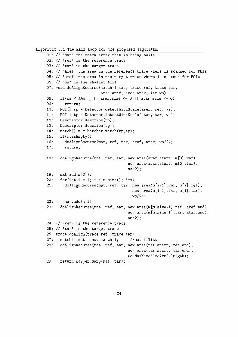
Algorithm 6.1 The main loop for the proposed algorithm

01: // 'mat' the match array that is being built

02: // 'ref' is the reference trace

03: // 'tar' is the target trace

04: // 'aref' the area in the reference trace where is scanned for POIs

05: // 'aref' the area in the target trace where is scanned for POIs

06: // 'ws' is the wavelet size

07: void doAlignRecurse(match[] mat, trace ref, trace tar,

area aref, area atar, int ws)

08: if(ws < Detmw || aref.size <= 0 || atar.size <= 0)

09: return;

10: POI[] rp = Detector.detectWithScale(aref, ref, ws);

11: POI[] tp = Detector.detectWithScale(atar, tar, ws);

12: Descriptor.describe(rp);

13: Descriptor.describe(tp);

14: match[] m = Matcher.match(rp,tp);

15: if(m.isEmpty())

16: doAlignRecurse(mat, ref, tar, aref, atar, ws/2);

17: return;

18: doAlignRecurse(mat, ref, tar, new area(aref.start, m[0].ref),

new area(atar.start, m[0].tar),

ws/2);

19: mat.add(m[0]);

20: for(int i = 1; i < m.size(); i++)

21: doAlignRecurse(mat, ref, tar, new area(m[i-1].ref, m[i].ref),

new area(m[i-1].tar, m[i].tar),

ws/2);

22: mat.add(m[i]);

23: doAlignRecurse(mat, ref, tar, new area(m[m.size-1].ref, aref.end),

new area(m[m.size-1].tar, atar.end),

ws/2);

24: // 'ref' is the reference trace

25: // 'tar' is the target trace

26: trace doAlign(trace ref, trace tar)

27: match[] mat = new match[]; //match list

28: doAlignRecurse(mat, ref, tar, new area(ref.start, ref.end),

new area(tar.start, tar.end),

getMaxWaveSize(ref.length);

29: return Warper.warp(mat, tar);

34

Figure 6.2.1: A power trace (top) with its points of interest for two scales (middle,bottom)

the minimum wavelet scale Detmw is reached. Due to the type of wavelet used (Mexicanhat) Detmw should be a multiple of 3.For performance reasons the wavelets are not applied for every sample but with a step

size of 10% of the wavelet scale. A small step size slows down the algorithm where as abig step size does not detect enough POIs to work with. Early testing showed promisingresults for a value of 10% but given the nature of the constant other values may work�ne as well.To be able to compare the responses to a threshold the responses are normalized with

respect to the wavelet scale. Samples with an absolute wavelet response less than Detthtimes the standard deviation of the trace, are discarded.A best-of-its-neighbors �lter is than applied to the remaining samples. If the absolute

wavelet response of a sample is not greater than the absolute wavelet responses of itsneighbors the sample is discarded. Neighbors are here de�ned as every sample within 3times the step size from the sample under evaluation. Early testing showed that at least3 times the step size is needed here, otherwise too many POIs come through the �lterand the matcher will not be able to di�erentiate them anymore. A greater window herecould also work but has not been researched.The samples that remain are the points of interest. Since these are the points that are

used for alignment later on it is important that they are located as accurate as possible.To achieve this the remaining responses are pin pointed by searching for the highestwavelet response in the vicinity (1 times the step size, otherwise this POI would not havebeen the best of its neighbors and would not have passed the �lter) of the point.Figure 6.2.1 shows the result of the detector. The �rst image is the original trace

35

followed by two images that show the POIs found by the detector at di�erent scales. Asis expected, large wavelets result in much fewer POIs than small wavelets. Therefore it iseasier to match the POIs from large scale wavelets to POIs from another trace. Howeversmaller wavelets give more information on how to align the traces.The type of wavelet used here de�nes on what patterns the responses will be high.

Searching for slope patterns (by using Haar wavelets) and for peak patterns (by usingMexican hat block wavelets) was used. Both wavelets are shown in �gure 4.3.1. TheMexican hat block wavelet outperformed the Haar wavelets in repeatability (it found thesame points in similar traces).Because the wavelet transform on a sample set comes down to multiplying every sam-

ple point of the wavelet with a sample point of the signal that is being analyzed, thecomplexity of applying a wavelet is usually O(n) with n being the scale of the wavelet.However when using block wavelets such as the Haar wavelet or the Mexican hat blockwavelet as shown in �gure 4.3.1 it can be done in O(1). First the trace is converted toa summed trace. Every sample is now the sum of itself and its predecessors. This isbased on the idea of integral images by Crow [8]. By subtracting two samples it is nowpossible to obtain the sum of all the samples in between. A convolution with a waveletis now calculated by multiplying the sum samples with the value of the block. A Haarwavelet can be applied with only 3 read operations on the trace regardless of its scale.The Mexican hat block wavelet needs only 4 read operations. Using the wavelets shownin 4.3.1 the mathematical formulas for getting a wavelet response on a sample array Aat position i with scale s look as follows:

Haar(A, i, s) =−(A[i]−A[i− s

2 ]) + (A[i+ s2 ]−A[i])√

s

=−2 ·A[i] +A[i− s

2 ] +A[i+ s2 ]√

s

Mexicanhat(A, i, s) =−(A[i− s

6 ]−A[i−s2 ]) + 2 · (A[i+ s

6 ]−A[i−s6 ])− (A[i+ s

2 ]−A[i+s6 ])√

s

=3 · (A[i+ s

6 ]−A[i−s6 ])− (A[i+ s

2 ]−A[i−s2 ])√

s

Note that the scaling with√s is not mandatory in general but is used here to compare

wavelet responses of di�erent scales.The code for a convolution with a Mexican hat wavelet can be seen in algorithm 6.2.

6.3 Descriptor

The descriptor aims to uniquely describe each POI by its context. It generates a featurevector which is used by the matcher to calculate the distance between two POIs. Thesefeatures must be robust to noise and because there are many POIs coming from one

36

Algorithm 6.2 Calculates the convolution of the Mexican hat block wavelet

01: // 'sa' is the sum array, sa[k] =∑k

i sample[i]02: // 'idx' is the position in the signal where the wavelet is applied

03: // 'ws' is the scale of the wavelet, which should be a multiple of 3

04: // return value is the response of the wavelet

05: double convoluteMexicanHatWavelet(double sa[], int idx, int ws)

06: int ts = ws / 3;

07: idx -= (ws+1) / 2; //add 1 to round upwards for odd ws

08: if(idx < 0 || idx+ws >= a.length)

09: return 0;

10: return (3.0*(sa[idx+2*ts]-sa[idx+ts])-(sa[idx+ws]-sa[idx])) / sqrt(ws);

Algorithm 6.3 The main procedure for the Detector.

01: // 'samples' is the sample array, which contains all sample points

02: // 'ws' is the scale of the wavelet, which must be a multiple of 6

03: return value is a list of POI positions

04: int[] doDetect(double samples[], int ws)

05: double sa[] = createSumArray(samples); //sum array

06: double ra[] = new double[sa.length]; //response array

07: int s = max(1, ws / 10); //stepsize

08: int[] ret = new int[]; //result variable

09: for(int i = 0; i < sa.length; i += s)

10: ra[i] = convoluteMexicanHatWavelet(sa, i, ws);

11: if(abs(ra[i]) < Detth*samples.sdev)12: ra[i] = 0;

13: for(int i = 0; i < sa.length; i += s)

14: if(ra[i] != 0 && isHighestOfItsNeighborPeaks(ra[i]))

15: ret.add(pinPointPeak(sa, i));

16: return ret;

37

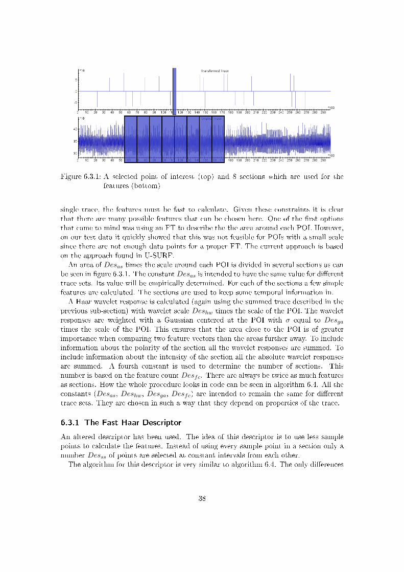
Figure 6.3.1: A selected point of interest (top) and 8 sections which are used for thefeatures (bottom)

single trace, the features must be fast to calculate. Given these constraints it is clearthat there are many possible features that can be chosen here. One of the �rst optionsthat came to mind was using an FT to describe the the area around each POI. However,on our test data it quickly showed that this was not feasible for POIs with a small scalesince there are not enough data points for a proper FT. The current approach is basedon the approach found in U-SURF.An area of Desas times the scale around each POI is divided in several sections as can

be seen in �gure 6.3.1. The constantDesas is intended to have the same value for di�erenttrace sets. Its value will be empirically determined. For each of the sections a few simplefeatures are calculated. The sections are used to keep some temporal information in.A Haar wavelet response is calculated (again using the summed trace described in the

previous sub-section) with wavelet scale Deshw times the scale of the POI. The waveletresponses are weighted with a Gaussian centered at the POI with σ equal to Desgatimes the scale of the POI. This ensures that the area close to the POI is of greaterimportance when comparing two feature vectors than the areas further away. To includeinformation about the polarity of the section all the wavelet responses are summed. Toinclude information about the intensity of the section all the absolute wavelet responsesare summed. A fourth constant is used to determine the number of sections. Thisnumber is based on the feature count Desfc. There are always be twice as much featuresas sections. How the whole procedure looks in code can be seen in algorithm 6.4. All theconstants (Desas, Deshw, Desga, Desfc) are intended to remain the same for di�erenttrace sets. They are chosen in such a way that they depend on properties of the trace.

6.3.1 The Fast Haar Descriptor

An altered descriptor has been used. The idea of this descriptor is to use less samplepoints to calculate the features. Instead of using every sample point in a section only anumber Desss of points are selected at constant intervals from each other.The algorithm for this descriptor is very similar to algorithm 6.4. The only di�erences

38

Algorithm 6.4 The main procedure for the Descriptor

01: // 'sa' is the sum array, sa[k] =∑k

i sample[i]02: // 'idx' is the position in the signal where the POI is found

03: // 'ws' is the scale of the wavelet

04: // return value is a list of features for the specified POI

05: double[] doDescribe(double sa[], int idx, int ws)

06: double f[] = new double[16]; //the feature vector

07: int da = Desas * ws; //the size of the description area

08: int sc = Desfc / 2; //section count

09: int ss = da / sc; //section size

10: int o = idx - sc/2 * ss; // offset, most left sample point

11: for(int s = 0; s < sc; s++)

12: f[2*s] = 0;

13: f[2*s+1] = 0;

14: for(int i = 0; i < ss; i++)

15: double t = convoluteHaarWavelet(sa, o+s*ss+i, Deshw*ws) *

Gauss(o+s*ss+i - idx, Desga);16: f[2*s] += t;

17: f[2*s+1] += abs(t);

18: return f;

are that after line 10 the following line is added:

int stepsize = max(1, ws / Desss);

And line 14 is replaced with:

for(int i = 0; i < ss; i+=stepsize)

6.3.2 The Super Fast Haar Descriptor

To further speed up the descriptor we assume that the Gaussian used in the descriptordoes not need to be continuous. By using a discretised version of the Gaussian functionwe get a block pattern which means we can apply the summed array trick here. For everyscale two sum arrays of the trace are calculated. One for the Haar wavelet responses andone for the absolute Haar wavelet responses. By subtracting two elements from these sumarrays it is possible to calculate the sum of the wavelet responses in between in O(1). Sucha summed block is then multiplied with the average of the Gaussian curve that wouldbe used in the normal descriptor for that block. Each block takes 2 read operationsand a multiplication with the Gaussian value to calculate. The number of blocks usedper section is de�ned by Desbs. More blocks means a more accurate Gaussian upto thevalue where Desbs equals the sample count per section. Then the Gaussian has the sameaccuracy as in the normal descriptor.

39

Algorithm 6.5 The main procedure for the Super Fast Haar Descriptor

01: // 'asr' is the sum array of the absolute wavelet responses

02: // 'sr' is the sum array of the wavelet responses

03: // 'idx' is the position in the signal where the POI is found

04: // return value is a list of features for the specified POI

05: double[] doDescribe(double asr[], double sr[], int idx)

06: double f[] = new double[16]; //the feature vector

07: int da = Desas * ws; //the size of the description area

08: int sc = Desfc / 2; //section count

09: int ss = da / sc; //section size

10: int bs = ss / Desbs; //block size

11: int o = idx - da/2; // offset, most left sample point

12: for(int s = 0; s < sc; s++)

13: f[2*s] = 0;

14: f[2*s+1] = 0;

15: for(int i = 0; i < Desbs; i++)

16: f[2*s] += sumArea(sr, o+s*ss+i*bs, o+s*ss+i*bs+bs) *

averageGuass(o+s*ss+i*bs, o+s*ss+i*bs+bs, Desga);17: f[2*s+1] += sumArea(asr, o+s*ss+i*bs, o+s*ss+i*bs+bs) *

averageGuass(o+s*ss+i*bs, o+s*ss+i*bs+bs, Desga);18: return f;

The code for this algorithm is shown in algorithm 6.5, it assumes that the two summedarrays for the wavelet responses are already calculated.

6.4 Matcher

The matcher creates a mapping between two sets of POIs. Because the results of thedetector and the descriptor are not perfect the matcher has to be robust to the fact thatnot every POI appears in every trace and that descriptions may be similar.For every POI from the reference trace a distance is calculated to every POI from the

target trace. To allow comparison against a threshold the normalized Euclidean distanceis used, which is a special case of the Mahalanobis distance and is de�ned by the followingformula:

d(−→x ,−→y ) =

√√√√ N∑i=1

(xi − yi)2σ2i

Where σi is the standard deviation of the xi over the sample set. In our case σi iscalculated using every possible POI with the same scale. In some cases, especially thosewith large scales, there are not enough POIs to give a proper estimate for σi but inpractice this does not cause problems.

40

Figure 6.4.1: Two matched POI sets, with Matmd = 1000 (left) and Matmd = 4(right)

Each POI from the reference trace is matched with the point with the lowest distanceof the target trace. If the distance is greater thanMatmd the match is removed. In thesecases the distance is so large that one could state that the matched points are not similarat all. Early testing showed that this removed most of the mismatches as can be seen in�gure 6.4.1. The traces used here were from a di�erent trace set than the one used inchapter 7 due to the fact that this was the only trace set available at the time.In the remaining matches there can still occur cross matches. By this we mean that

sample point refn of the reference trace is matched against sample point tarn of thetarget trace while at the same time sample refn+p is matched against sample tarn+qwith p · q < 0. This cannot be allowed because it would violate the temporal behaviorof the trace. This is the same constraint that is given with Elastic Alignment: thetrace can be stretched and shrunk but not folded. To resolve these cross matches thecon�dence of a match and a penalty function is used. The con�dence of a match isde�ned by the distance of the best match divided by the distance for the second bestmatch. The penalty function halves the con�dence of a match for every other match itcrosses. The con�icting match with the lowest con�dence is then removed from the set.This is repeated until all cross matches are resolved. A pseudo code implementation isshown in algorithm 6.6 and 6.7.

6.5 Warper

The Warper takes a list of matched POIs from two traces and shrinks and stretchesthe target trace so it is aligned with the reference trace. In the result trace the valuesof the samples that are included in the match list are set to the values of the target-trace. Values in between the matched points are interpolated. Various interpolationschemes have been tried such as Nearest Neighbor, Linear, Cosine, Cubic and Hermite[6]. Hermite interpolation is similar to cubic but has tension and biasing parameters.The tension controls tightens the curve at known points whereas bias twists the curvetowards one of the two points. Early testing showed that di�erences were minimal butslightly in favor of the Cubic interpolation scheme. The other schemes have not beenresearched further.

41

Algorithm 6.6 The violator function

01: // 'mat' is the list of matches

02: // 'idx' is the index where the conflict was detected

03: int findViolator(match[] mat, int idx)

04: match[] v = selectMatchesCrossedBy(mat, idx); //matches that cause problems

05: double mc = infinity; //lowest confidence thusfar

06: int mm = 0

07: for(int i = 0; i < v.length; i++)

08: double c = v[i].confidence;

09: c *= pow(0.5, countCrossMatches(mat, i));

10: if(c < mc)

11: mc = c;

12: mm = i;

13: return i;

The start and the end of the traces are not necessarily aligned. The samples before the�rst matched sample are interpolated with the same parameters as the samples betweenthe �rst and the second matched samples. The same is done at the end of the trace.Sometimes a gap remains at the start or end of an aligned trace. There are multiplevalues that can be used to �ll such a gap. One can use zeroes, copy parts of the referencetrace or use the value of the nearest sample. The best results were achieved by usingthe values of the nearest sample. This is due to the fact that it does not disturb thecontinuity of the trace as zeroes would do and it does not add patterns that should notbe there as copying from the reference trace would do. The pseudo code is shown inalgorithm 6.8.

42

Algorithm 6.7 The main procedure for the Matcher

01: // 'ref' is the list of POIs found in the reference trace

02: // 'tar' is the list of POIs found in the target trace

03: match[] doMatch(POI[] ref, POI[] tar)

04: double d1 = infinity; //shortest distance

05: double d2 = infinity; //second shortest distance

06: POI pm = null; //POI with distance d1

07: double c = 1; //confidence for the match

08: match[] ret = new match[];

09: forall(POI p in ref)

10: forall(POI q in tar)

11: double d = getNormalizedEuclideanDistance(p, q);

12: if(d < d1)

13: d2 = d1;

14: d1 = d;

15: pm = q;

16: elseif(d < d2)

17: d2 = d;

18: if(d2 < infinity)

19: c -= d1 / d2;

20: if(d1 < Matmd)21: ret.add(new match(p, pm, c));

22: //resolve conflicts

23: for(int i = 0; i < ret.length; i++)

24: if(crossesAnyOtherMatch(ret[i])

25: ret.remove(findViolator(ret, i));

26: i = 0;

27: return ret;

43

Algorithm 6.8 The main procedure for the Warper

01: // 'mat' is the list of matches

02: // 't' is the trace currently being aligned

03: trace doWarp(match[] mat, trace t)

04: trace ret = new trace();

05: addArtificialMatchesStartEnd(mat);

06: for(int m = 1; m < mat.length; m++)

07: int ddest = mat[m].refpos - mat[m-1].refpos; //delta in refrence trace

08: int dsrc = mat[m].tarpos - mat[m-1].tarpos; //delta in target trace

09: double r = dsrc / ddest; // stretch/shrink factor

10: for(int i = 0; i < ddest; i++)

11: ret[mat[m].refpos + i] = interpolatedPoint(t, mat[m].tarpos + i*r);

12: ret[ret.length-1] = t[t.length-1];

13: return ret;

44

7 Experiments

The performance of the proposed algorithm was measured through several experiments.The set up for these experiments is similar to what was used by Hogenboom in [11],this set up can be seen in �gure 7.0.1. The main di�erences are that here a di�erentoscilloscope is used and the device-under-attack is di�erent. The detailed hardware andsoftware requirements as well as the general setup are explained in the remainder of thischapter.

7.1 Hardware

The hardware used for our measurements consists of several components which are listedbelow.

Power tracer This device is an advanced smartcard reader which can be connected to anoscilloscope. It is developed by Riscure B.V. and is controlled via the software toolInspector. The power tracer can trigger the oscilloscope so the amount of unusablesamples is reduced. It also has a very low noise power supply for the smart cardwhich improves the signal to noise ratio.

Oscilloscope To measure the power usage of a device one needs an oscilloscope. For thisproject the LeCroy 104Xi was used. This is a Windows based oscilloscope that canmeasure up to 10 gigasamples per second and has a low noise �gure.

Filters An analog �lter was used to �lter out frequencies that would not contribute tothe CPA. In this case we used a lowpass 48Mhz �lter which reduces the amplitudeof the high frequencies and allows the low frequencies to pass through.

Smartcard The traces that were used for this project were acquired from a cards providedby Riscure. They contained a software implementation of Triple DES (used herewith k1 = k2, so it becomes a normal DES) with countermeasures which could beturned on and o�. For this project the only countermeasure that was turned onwas random delays.

Computer Finally there is a computer needed to link everything together. Although thetraces and calculations were performed on several computers the calculation timemeasurement was done on a computer with an E6750 2.66Ghz processor and 2Gbof RAM memory.

45

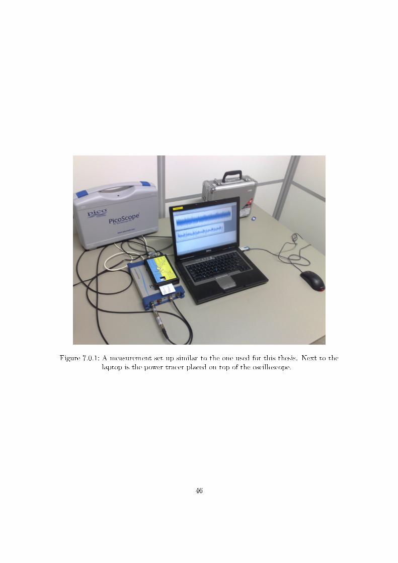
Figure 7.0.1: A measurement set up similar to the one used for this thesis. Next to thelaptop is the power tracer placed on top of the oscilloscope.

46

7.2 Software and Settings

The main tool used for this project is an application called 'Inspector'. This is a tooldeveloped by Riscure B.V. speci�cally designed to handle any operations needed forside channel analysis. When this tool is combined with the right hardware it can beused to acquire samples for analysis. These samples can be power measurements orelectromagnetic measurements. Samples can also be inspected and analyzed with variousmodules that come with the product. The version used for this project and also currentlythe latest version is 4.3. Several modules where used to �lter the data set before aligning.The following modules were used for this thesis:

DESAcquisition Module

This module is used in combination with the oscilloscope and powertracer to gathertraces from an electronic device, in our case a smartcard. The module dialog showsvarious settings for the oscilloscope and the power tracer. The most notable settings forthe oscilloscope are: the sample frequency, number of samples and delay.The sample frequency speci�es how many samples per second should be taken. Higher

frequencies give more detail but use more disc space to store. The frequency should beset to at least the clock speed of the smartcard, 4Mhz in our case. If the sample rateis lower than the clock speed, di�erent clock cycles end up in one sample and valuableleaked information might get lost. This setting was set to 250 megasamples per second.We chose for a much higher frequency than the clock speed to get a more accuratereading per clock cycle. The acquired traces were resampled right after acquisition bythe Resample module.The number of samples speci�es how many samples are acquired per trace. It is

important that this enough to cover one round of the encryption procedure. If it is toolow and critical parts are missing it is impossible to do a successful CPA attack. We chosea number much greater than we anticipated we would need. Afterwards we cropped thepart of the trace that was actually useful. This resulted in traces of 8248 samples long.If a delay is set the oscilloscope waits with sampling until it receives a trigger from

the powertracer. In our case the trigger was sent right after the input bytes for theencryption algorithm were transmitted.There are also some settings for the powertracer. The most notable here is the number

of traces that should be acquired. In order to generate graphs based on statistics a largenumber of traces is required. We set this setting to 500,000 (�ve hundred thousand)traces.

Resample Module

Right after the acquisition before writing them to the disc the traces were resampledin order to save disc (and memory) space. This module resamples a trace by averagingconsecutive samples. We resampled to 4 megasamples per second (the clock speed of thesmartcard). This resulted in a data set of 16 gigabytes. We set this module to align to apeak (clock pulse) before starting to average. This ensures that for every trace in the setthe resample window is more or less positioned the same way. Otherwise one could have

47

Figure 7.2.1: A typical trace from the data set, showing the last round of the encryption

the clock pulse in the beginning of the window in one trace and at the end in another.When traces are combined leakage information is spread over multiple clock cycles anbecome much harder to retrieve. A typical trace from the resulting set is shown in �gure7.2.1. Note that the y-axis shows negative mVolts. This is due to an o�set error duringacquisition and has no consequences for this thesis.

StaticAlign Module

This module was used to align the traces in the set so we could compare our proposedalgorithm to Static Alignment. This module implements Static Alignment as is describedin chapter 3. We selected a trace fragment of 600 samples at the end of the encryptionwhere the module should align on. The allowed shift for this fragment was set to 250samples.

CombAverage Module

This module pre-processes the traces for a SW-DPA attack. It averages the samples asdescribed previously after which a normal DPA attack can be performed. The modulehas two settings: the number of samples per clock cycle which is set to 1 and the size ofthe sliding window for which we used the values 50, 100 and 200.

ElasticAlign Module

This module was used to align the traces in the set so we could compare our proposedalgorithm to Elastic Alignment. This module implements Elastic Alignment as is de-scribed in chapter 3. This module has a settings to set the radius in which FastDTWsearches for the optimal warppath. We set this setting to auto con�gure. The modulethen selects the optimal settings based on the �rst few traces. The optimal radius foundwas 70.

RAMAlign

This is a custom module that implements our proposed algorithm. In the settings dialogall the constants introduced in chapter 6 are listed and can be changed. As a baselinethe initial values of the constants were chosen close to the values of U-SURF [3] wherepossible. The other baselines for the constants were based on early experimentation.Then the values where changed and used for a fraction of the data set. Based on theaverage Pearson correlation of the target traces with the reference trace it was decidedwhether increasing the value or decreasing it would show more promise. If the traceswould be good aligned they would show a higher correlation than the baseline and if thetraces would not be aligned properly the correlation would be lower than the baseline.

48

However since high correlation does not directly indicate a proper alignment in somecases it was decided that both a higher value and a lower value for the constants shouldbe analyzed.The analysis was done by the FirstOrderAnalysis module. Which was used to give a

more founded argument for the speci�c values for the constants. Here are the constantslisted with a short description and the values that were tested. The baseline values arein bold.

Minimum Wavelet Size (Detmw) This constant speci�es the stopping criterion for thedetector. The detector starts with large wavelets and decreases them everyiteration. If this wavelet size is reached the detector is done. Besides thatlowering this value increases computation time, usually there are much morepossible POIs at low wavelet sizes. This could confuse the matcher. On theother hand, lowering this value provides more precision for alignment andcould increase the overall score. Tested values: 3, 6 and 12.

Response Threshold (Detth) The detector only selects samples to become potentially aPOI if the wavelet response at that point is greater than Detth times thestandard deviation of the trace. A higher value causes less confusion for thematcher but may result in too few POIs to do proper alignment. A lowervalue has also increases the running time of the algorithm. The matchingalgorithm is quadratic in the number of POIs detected so which makes thisvery computationally very demanding. Tested values: 2, 2.5 and 3.

Area Size (Desas) This speci�es the size of the area around the POI which is used for thegeneration of the feature vector for this POI. The area of this POI is Desastimes the scale of the POI. Low values mean that POIs are related to eachother based on the samples close to the POI (which could have patterns thatexist multiple times in the trace). High values take samples further away intoaccount, but could cause confusion that due to the fact that areas of POIsoverlap too much. Tested values: 12, 16 and 20.

Feature Count (Desfc) This constant is related to the area size. It speci�es how manyfeatures should be calculated in the speci�ed area. More features meanslonger computation time but more accuracy when relating POIs. Testedvalues: 16, 24 and 32.

Haar Wavelet Size (Deshw) The descriptor uses Haar wavelets of size Deshw times thescale of the POI to generate the feature vectors. Higher values means search-ing for patterns (slopes in this case) in lower signal frequencies. The waveletbecomes bigger and is less sensitive for small frequencies. Tested values: 1.5,and 2.5.

Standard Deviation Gaussian (Desga) The descriptor weighs the Haar wavelet responseswith a Gaussian with an standard deviation of Desga times the scale of thePOI. The Gaussian is centered at the POI. Lowering the value of this constant

49

means that the description is focused on samples closer to the POI. Increasingthe value widens the focus window of the description. Tested values: 2.8, 3.3and 3.8.

Maximum Distance (Matmd) This constant speci�es the maximum allowed distance be-tween two matched POIs. If a match has a distance of more than Matmd itis discarded. Lowering this value prevents cross matching. Lowering it toomuch discards usable matches. Tested values: 2.3, 2.5 and 2.7.

Due to the fact that some of the constants in�uence each other, changing the settingon one constant may change the optimal settings for the others, it is hard to �nd goodvalues. A full grid search over all plausible combinations would take too much time sowe chose to pick a base line and tune one constant at the time.

FirstOrderStatisticalAnalysis Module

This is a statistical custom module by Jasper van Woudenberg (supervisor) it is usedto measure the performance of an pre-processing algorithm in combination with a CPAattack. After pre-processing is done (in our case this is the aligning) it splits up the traceset into subsets. For each subset a number of traces Ns is selected and a CPA attack isperformed on these traces. The module counts the number of successful attacks S+ andthe number of unsuccessful attacks S− and calculates the �rst order success rate Rs:

Rs =S+

S+ + S−

Rs is then reported as a percentage of success for this speci�c number of traces. Ns

is then increased and the process is repeated. This results in a climbing percentage ofsuccess the more traces are added. This is an indication of, given the pre-processingmethod, how many traces would be needed to get a certain percentage of success.We set the start number of traces to 100 and the end to 5000 with a step size of 100.

This means the data set is split into 500, 000/5000 = 100 subsets and that the modulereturns 50 data points per full execution. A full execution on takes about 9 hours on thisdata set pre-processing not included.

7.3 Tuning Results

Every execution of the FirstOrderStatisticalAnalysis module results in a series of datapoints. For every constant these data points were plotted in a graph as can be seen in�gure 7.3.1. In every graph the baseline is plotted with a black dotted line.When looking at the resulting graphs one of the �rst things that can be concluded

is that the chosen baseline is not a particularly high performer. This is not a problemthough, since it is here only used to tune the constants. Another important thing to noteis that one should expect the graphs to be rather smooth and monotonically increasing.This is because each added trace contains leaked information that, when successfullyextracted, should contribute to a higher success ratio. However the graphs are not

50

smooth and some start to decrease after a number of traces. This is due to the factthat if alignment for a trace fails completely it takes many successfully aligned tracesto average out the errors. When more traces are used the chance of such a 'bad' traceincreases and causes the success rate to drop.There are two ways to counter this. The �rst is to improve the algorithm so it produces

less (or none) of these bad traces. This solution is implemented by using tuned values forthe constants. The second way is to build in a detection mechanism that discards badtraces. This can be implemented by using Pearson correlation after the trace is aligned.If the correlation result is below a certain threshold the trace is discarded. However, itis possible to use �lter for any alignment algorithm therefore it is not considered part ofthe algorithm here. The correlation �lter is not used during the experiments here sinceit would mask the performance of the actual algorithm.The results from the graph are discussed per graph.

Minimum Wavelet Size This graph shows a clear increase in performance when using thesmallest possible wavelet of scale 3.

Response Threshold Here there is clear improvement when the number of POIs increases.When too much POIs are allowed the matcher gets confused and performancedrops drastically. This can be seen with the threshold value of 2.

Area Size This graph suggests that there is too much overlap in the descriptions of thePOI and that the area size should be lowered.

Feature Count The results here are inconclusive. There is a very small di�erence in favorof less features. However, this could be noise. In early testing we were ableto make a CPA attack work by increasing the number of features and sincethis graph does not give enough reason to lower the value of this constantremains at the baseline setting of 32.

Haar Wavelet Size Here the graphs show di�erences slightly in favor of the baseline set-ting of 2.

Gaussian Standard Deviation Here we were too careful with changing the value. Theperformance di�erences are very minimal but it is slightly in favor of a widerGaussian curve. This suggests that the actual description is focused too muchon samples close to the POI.

Maximum Distance Here we have been too careful with changing the value as well. Fromearly testing it was very clear that a high maximum distance would cause adrop in performance. However this does not show up in the graph. Since theThreshold graph suggests that more POIs would be better for alignment itwill probably not hurt to lower this setting slightly so only the best matchesare used.

After we set the parameters to the new values the success ratio increased greatly ascan be seen in �gure 7.3.2. This performance is su�cient enough to be useful in practice.

51

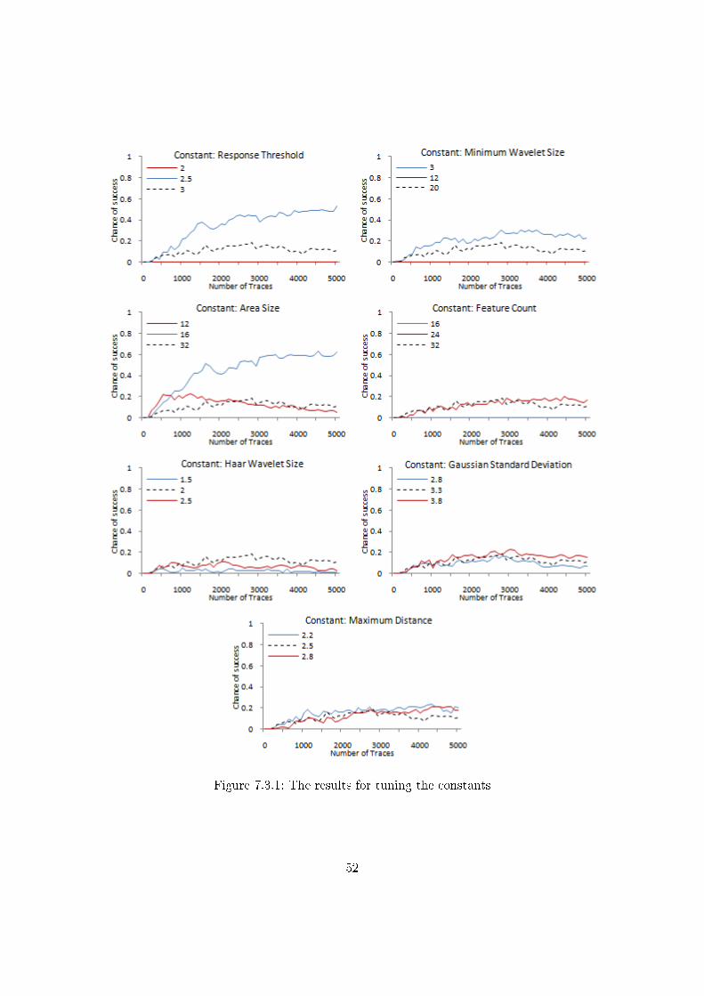
Figure 7.3.1: The results for tuning the constants

52

Figure 7.3.2: The performance of the tuned version

Component Time of Calculation (%)

generateFeatures() 32

getEucledianDistance() 21.6

convoluteHaarWavelet() 20.4

getFeature() 15.8

getGaussian() 4.3

... 5.9

Table 7.1: Top 5 CPU intensive functions

Although further tuning might further increase the success ratio the focus was shifted tospeed.

7.4 Speed Boosting Results

To �nd out where the algorithm spent the most time during execution it was passedthrough the Netbeans pro�ler. The top �ve most demanding functions are shown intable 7.1. The �rst, third and �fth function in the table are both used in the descriptor.This means that the descriptor consumes 56.7% of the CPU cycles. Our �rst attempt tospeed up the algorithm is by using a faster descriptor.

7.4.1 The Fast Haar Descriptor

The Fast Haar descriptor introduces a new constant:

53

Figure 7.4.1: Results of the Fast Haar Descriptor

Samples Per Section (Desss) This is the number of samples used per section. The moreare used the better the descriptor describes that section. If signi�cantly lessare used it speeds up the algorithm. Tested values: 10 and 20.

The results from this run are shown in �gure 7.4.1. The number of selected samples persection does not seem to in�uence the success rate with the chosen values. Although thismight be di�erent on noisier trace sets, for this trace set it means that this descriptorperforms well enough for use in practice. The run time on our test computer is shown intable 7.2. Although the speed increase is signi�cant there is more to gain as is shown inthe next subsection.

7.4.2 The Super Fast Haar Descriptor

The Super Fast Haar descriptor introduces a new constant:

Blocks Per Section (Desbs) This is the number of blocks to calculate per sample. Ahigher value means that the result comes closer to that of a continuous Gaus-sian curve. Lower values speed up the calculation. Tested values: 1 and2

From the results shown in �gure 7.4.2 it is clear that the performance is decreased.Although the algorithm gained a great speed boost as is shown in table 7.2 the FastHaar Descriptor may be preferred on more di�cult trace sets.

54

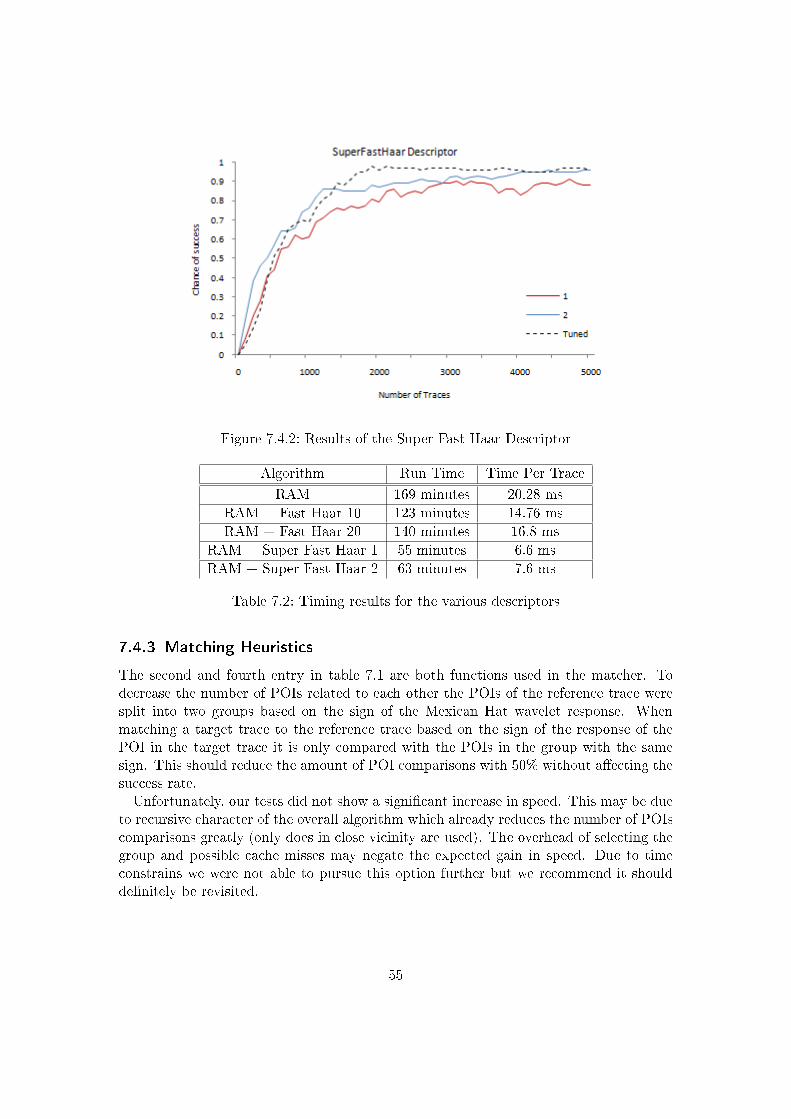
Figure 7.4.2: Results of the Super Fast Haar Descriptor

Algorithm Run Time Time Per Trace

RAM 169 minutes 20.28 ms

RAM + Fast Haar 10 123 minutes 14.76 ms

RAM + Fast Haar 20 140 minutes 16.8 ms

RAM + Super Fast Haar 1 55 minutes 6.6 ms

RAM + Super Fast Haar 2 63 minutes 7.6 ms

Table 7.2: Timing results for the various descriptors

7.4.3 Matching Heuristics

The second and fourth entry in table 7.1 are both functions used in the matcher. Todecrease the number of POIs related to each other the POIs of the reference trace weresplit into two groups based on the sign of the Mexican Hat wavelet response. Whenmatching a target trace to the reference trace based on the sign of the response of thePOI in the target trace it is only compared with the POIs in the group with the samesign. This should reduce the amount of POI comparisons with 50% without a�ecting thesuccess rate.Unfortunately, our tests did not show a signi�cant increase in speed. This may be due

to recursive character of the overall algorithm which already reduces the number of POIscomparisons greatly (only does in close vicinity are used). The overhead of selecting thegroup and possible cache misses may negate the expected gain in speed. Due to timeconstrains we were not able to pursue this option further but we recommend it shouldde�nitely be revisited.

55

Figure 7.4.3: The algorithm without Gaussian (Left) without pinpointing (Right) andwith Nearest Neighbor interpolation (Right)

7.4.4 Simpli�cations

When the �rst version of the algorithm was designed a lot of design choices were basedon the U-SURF paper and on early testing. Here more extensive testing is used to seewhether all computation steps are necessary. Time constrains limited the number of teststhat could be performed here but some interesting results were found nonetheless. Othertests suggested that increasing the standard deviation of Gaussian used in the descriptorincreases performance of the algorithm. This means that looking at samples close to thePOI may not be the best way to match them to POIs in other traces. The Gaussianweighting function was removed and the results are shown in the left graph in �gure7.4.3. The graph shows an increase in performance for both the Fast and Super FastHaar descriptors. This means that either the values that have been used thus far for thestandard deviation of the Gaussian were way too low or the Gaussian is not needed atall. The gain in success rate also comes with a speed boost for the Fast Haar descriptoras can be seen in table 7.3.Other choices that were based on early testing were the use of a pinpointing method

and the choice of the interpolation scheme of the warper. Instead of using pinpointingto �nd the precise position of a POI one may assume that the precision of 10% of thewavelet scale would su�ce. The right graph in �gure 7.4.3 shows that there is a slight butsigni�cant performance drop when not using pinpointing. The timing results in table 7.3show that instead of reducing the time to process the traces it took longer. This couldbe due to the fact that the feature vectors of the POIs are of lesser quality causing themore cross matching to solve for the matcher.From the same �gure and table can be seen that choosing a nearest neighbor interpola-

tion scheme for the warper slightly lowers performance. The reduction in processing timealso slightly decreases but since in practice it is more important to gain a little higherchance of success than a few minutes in time Cubic interpolation scheme is preferred.

56

Algorithm Run Time Time Per Trace

RAM + Fast Haar 10 + No Gauss 76 minutes 9.1 ms

RAM + Super Fast Haar 1 + No Gauss 54 minutes 6.5 ms

RAM + Fast Haar 10 + Nearest Neighbor 121 minutes 14.6 ms

RAM + Fast Haar 10 + No Pinpointing 116 minutes 13.9 ms

Table 7.3: Timing results for the simpli�cation attempts

Algorithm Run Time Time Per Trace

Static Alignment 12 minutes 1.44 ms

SW-DPA 18 minutes 2.16 ms

RAM + Super Fast Haar + No Gauss 63 minutes 7.6 ms

RAM + Fast Haar + No Gauss 76 minutes 9.1 ms

Elastic Alignment 3115 minutes 373.8 ms

Table 7.4: Timing results for the various alignment methods. The time listed for SW-DPA is the additional time it took to perform the DPA attack

7.5 Comparison Results

The algorithms that resulted from the experiments was compared to Elastic Alignment,Static Alignment and SW-DPA. The results are shown in �gure 7.5.1. The graph on theleft shows that our proposed algorithm performs slightly worse than Elastic Alignmentfor low number of traces. Static Alignment and SW-DPA are not able to overcome thecountermeasures within 5000 traces.Since our main goal was to design an algorithm that was much faster than Elastic

Alignment we compared the running times of the algorithms. The results are shown intable 7.4. Our proposed algorithm performs much faster than Elastic Alignment. Sowhen time is a factor this clearly is the algorithm of choice.To further express the potential of this algorithm the success-to-minute ratio was

calculated from the already available data. To give a clear picture of the advantage ofRAM over Elastic Alignment the data needed to be transformed and interpolated. Thethe chance of success after a certain number of minutes is plotted in �gure 7.5.1. Inthe graph on the right can be seen that RAM achieves success rates of over 95% in 30minutes where Elastic Alignment would take over 32 hours to do the same.

57

Figure 7.5.1: Success To Trace Ratio (Left) and Success to Time Ratio (Right). Notethat data points in the right graph are not measurements but translatedand interpolated points from other experiments.

58

8 Conclusion

8.1 Conclusion

Di�erential Power Analysis is a widely used side channel attack that uses leakage in thepower signal of a device to extract its secret key. It requires a large number of power signalmeasurements of the device while it is encrypting known plaintexts and uses statistics toanalyze them.For this attack to work it is important that power traces are aligned in the time domain.

If this is not the case the number of traces required to successfully perform the attackincreases with several orders of magnitude. One of the countermeasures against thistype of attacks is based on this requirement. By using an unstable clock or introducingdummy operations the measurements are misaligned.Although several algorithms exist to align the measurements they are all limited in

either success-to-number-of-traces-ratio or computation time. We introduce a fast algo-rithm with a reasonable success ratio. We used a smartcard with a software implemen-tation of triple DES to measure the performance of the algorithm.We used several experiments to tune the parameters of the algorithm. All of these

parameters are dependent on properties of the traces to be aligned. This results in analgorithm which is easy to use for an attacker since there are no parameters that needtuning. Although our tuning e�orts resulted in reasonable results it is very well possiblethat further tuning increases performance even more.We compared our proposed algorithm with Static Alignment, Sliding Window DPA and

Elastic Alignment. While Static Alignment and Sliding Window DPA are not capableof properly aligning the used trace set, Elastic Alignment showed excellent performancebut was relatively slow. It took almost 52 hours to process the 500,000 traces from ourdata set. Our proposed algorithm performed similarly in terms of success ratio comparedto Elastic Alignment but took only 76 minutes to process the data set.The proposed algorithm consists of four components. Each of these components can

be replaced so that new approaches can easily be tested. This provides an easy to useframework for alignment algorithms.At his moment the matcher component is the weakest link. The algorithm detects

points of interest of di�erent scales to align the traces with. If a mismatch occurs betweentwo traces with points of a large scale the resulting trace is not be usable. A bettermatching scheme may prevent this.We conclude that RAM Alignment outperforms all of its competitors: WS-DPA, Static

Alignment and Elastic Alignment1.

1Near the end of writing this thesis, Riscure reported they developed a new version of Elastic Alignment

59

8.2 Further research and suggestions

Although our proposed algorithm already outperforms it competitors, there are still someopen ends. In this section is brie�y discussed what topics could be interesting for furtherresearch.One of the most important di�erences between modern smartcards and the smartcard

used for testing is that modern smartcards have signi�cantly more noise in there powersignal. It would be interesting to know how well the proposed algorithm reacts to suchnoise. To do this similar tests could be run on smartcards with di�erent noise pro�lesand other countermeasures enabled.To boost the success rate of the algorithm it would de�nitely be interesting to further

tune the constants. The tuning so far has shown an increase in the success rate fromabout 20% to 95-100%. With more extensive tuning it might be possible to achieve thesesuccess rates with less traces.To boost the speed of the algorithm the focus should be on the matcher as this is

currently the most demanding component in the algorithm. To lower the O(n2) in thatcomponent one could sort the POIs selected for matching based on their distance to theorigin, the distance to a description vector with only zeroes. In that way it is possible todiscard of POIs that de�nitely fall outside the maximum distance range in O(nlog(n)).This lowers the amount of POIs that are related to each other in the O(n2) part of thealgorithm.Splitting the POIs of the reference trace into two groups based on whether the Mexican

Hat wavelet response was positive or negative could decrease the number of POIs relatedto each other with 50%. We did some experiments with this but it the results wereinconclusive. It is recommended to revisit this option.After the sumtrace is calculated most operations are done independent to each other.

This allows for parallel computing which could greatly improve the calculation time.Also the application of the algorithm allows for easy use of parallel computing. Since thetraces are processed independently only being compared with the reference trace (readoperations only) it is possible to assign di�erent parts of the trace set to di�erent threadswithout much overhead.Now, for matching the POIs are selected based on their position in the trace (they

are selected based on the POIs found on the previous (larger) scale). Instead, the POIsof the reference trace could be stored in a kd-tree-like structure. This returns POIs innearest-neighbor-�rst order. To built such a tree takes O(nlog(n)). This will cause a lotmore cross matches that need to be dealt with, on the other hand it might be possible torecover from mismatches at higher scales since they are no longer used to select potentialgood POI matches. Right now if a mismatch occurs at a large scale all lower scales gowrong too.In order to make the algorithm easy to use all of the parameters are depending on

properties of the trace. However, some (the detection of POIs) depend on the standarddeviation of the trace. This is not ideal since some traces contain patterns that are

which is about 3 times faster than the implementation used in this thesis.

60

not part of the encryption, often due to communication, that signi�cantly increase thestandard deviation. To overcome this properly one could select a part of the trace overwhich the standard deviation should be calculated instead of the full trace.Last but not least, di�erent detector and description schemes could be used to in-

crease the aligned trace quality. This fundamentally changes the algorithm but thedetector-descriptor-matcher-warper-framework proposed here could be useful in manycon�gurations.

61

Bibliography

[1] J. Allen. Short term spectral analysis, synthesis, and modi�cation by discreteFourier transform. Acoustics, Speech and Signal Processing, IEEE Transactionson, 25(3):235�238, 2003.

[2] D. Ballard. Generalizing the hough transform to detect arbitrary shapes. Patternrecognition, 13(2):111�122, 1981.

[3] H. Bay, T. Tuytelaars, and L. Van Gool. Surf: Speeded up robust features. ComputerVision�ECCV 2006, pages 404�417, 2006.

[4] J. Beis and D. Lowe. Shape indexing using approximate nearest-neighbour searchin high-dimensional spaces. In Computer Vision and Pattern Recognition, 1997.Proceedings., 1997 IEEE Computer Society Conference on, pages 1000�1006. IEEE,1997.

[5] E. Brier, C. Clavier, and F. Olivier. Correlation power analysis with a leakage model.Cryptographic Hardware and Embedded Systems-CHES 2004, pages 135�152, 2004.

[6] R. Burden and J. Faires. Numerical analysis. 2004. Brooks Cole, Paci�c Grove,California, United States.

[7] C. Clavier, J. Coron, and N. Dabbous. Di�erential power analysis in the presenceof hardware countermeasures. In Cryptographic Hardware and Embedded Systems-CHES 2000, pages 13�48. Springer, 2000.

[8] F. Crow. Summed-area tables for texture mapping. ACM SIGGRAPH ComputerGraphics, 18(3):207�212, 1984.

[9] J. Fourier. Théorie Analytique de la Chaleur, 1822. Firmin Didot�Père et Fils (nowpublic domain, scanned by Google) Fourier-Théorie Analytique de la Chaleur. pdf.

[10] F. Garcia, G. de Koning Gans, R. Muijrers, P. Van Rossum, R. Verdult, R. Schreur,and B. Jacobs. Dismantling MIFARE classic. Computer Security-ESORICS 2008,pages 97�114, 2008.

[11] J. Hogenboom. Principal Component Analysis and Side-Channel Attacks, MSc The-sis Nr 634. 2010.

[12] P. Kocher, J. Ja�e, and B. Jun. Di�erential Power Analysis. In Advances incryptology-CRYPTO'99: 19th Annual International Cryptology Conference, Santa

62

Barbara, California, USA August 15-19, 1999 proceedings, page 388. Springer BerlinHeidelberg, 1999.

[13] D. Lowe. Object recognition from local scale-invariant features. In ICCV, page 1150.Published by the IEEE Computer Society, 1999.

[14] S. Mangard, E. Oswald, and T. Popp. Power analysis attacks: Revealing the secretsof smart cards. Springer Verlag, 2007.

[15] T. Messerges. Using second-order power analysis to attack DPA resistant software. InCryptographic Hardware and Embedded Systems-CHES 2000, pages 27�78. Springer,2000.

[16] K. Mikolajczyk and C. Schmid. Indexing based on scale invariant interest points.In Computer Vision, 2001. ICCV 2001. Proceedings. Eighth IEEE InternationalConference on, volume 1, pages 525�531. IEEE, 2001.

[17] A. Moradi, M. Shalmani, and M. Salmasizadeh. Dual-rail transition logic: A logicstyle for counteracting power analysis attacks. Computers & Electrical Engineering,35(2):359�369, 2009.

[18] N. Ricker. Wavelet contraction, wavelet expansion, and the control of seismic reso-lution. Geophysics, 18:769, 1953.

[19] S. Salvador and P. Chan. FastDTW: Toward accurate dynamic time warping inlinear time and space. In KDD Workshop on Mining Temporal and Sequential Data,pages 70�80, 2004.

[20] K. Tiri, M. Akmal, and I. Verbauwhede. A dynamic and di�erential CMOS logic withsignal independent power consumption to withstand di�erential power analysis onsmart cards. In Solid-State Circuits Conference, 2002. ESSCIRC 2002. Proceedingsof the 28th European, pages 403�406. IEEE, 2002.

[21] K. Tiri and I. Verbauwhede. A logic level design methodology for a secure DPAresistant ASIC or FPGA implementation. In Proceedings of the conference on De-sign, automation and test in Europe-Volume 1, page 10246. IEEE Computer Society,2004.

[22] J. van Woudenberg, M. Witteman, and B. Bakker. Improving di�erential poweranalysis by elastic alignment. Topics in Cryptology�CT-RSA 2011, pages 104�119,2011.

63