Rainfall in Queensland - CentAURcentaur.reading.ac.uk/67985/2/klingaman_qldrain_part3.pdf · Rainfall in Queensland Part 3: ... Seasonal- and annual-mean timeseries of indices correlated

Rainfall in Queensland

Part 3: Empirical Orthogonal Teleconnection analysis of inter-annual variability in Queensland rainfall Understanding the influence of atmospheric drivers Prepared by Nicholas Klingaman

February 2012

i

Prepared by: Nicholas P. Klingaman, Walker Institute for Queensland Climate Change Centre of Excellence, Department of Environment and Resource Management GPO Box 2454 Brisbane Qld 4001 © The University of Reading 2012 Copyright inquiries should be addressed to <[email protected]> ISBN 978-0-9750827-4-4 Disclaimer

This document has been prepared with all due diligence and care, based on the best available information at the time of publication. The department holds no responsibility for any errors or omissions within this document. Any decisions made by other parties based on this document are solely the responsibility of those parties. Information contained in this document is from a number of sources and, as such, does not necessarily represent government or departmental policy. If you need to access this document in a language other than English, please call the Translating and Interpreting Service (TIS National) on 131 450 and ask them to telephone Library Services on +61 7 3224 8412. This publication can be made available in an alternative format (e.g. large print or audiotape) on request for people with vision impairment; phone +61 7 3224 8412 or email <[email protected]>. This report should be referenced as: Klingaman, N.P., 2012: Empirical orthogonal teleconnection analysis of interannual-variability in Queensland rainfall. QCCCE Research Report [number]. Department of Environment and Resource Management. Available online at www.derm.qld.gov.au. Acknowledgements

Dr Nicholas Klingaman was funded by a grant from the Queensland Government, under a collaboration between the Queensland Climate Change Centre of Excellence (QCCCE) and the Walker Institute. Dr Klingaman was supervised by Steve Woolnough of the Walker Institute and Jozef Syktus of QCCCE. Dr Klingaman acknowledges productive discussions on EOT analysis with Ian Smith of the Commonwealth Scientific and Industrial Research Organisation. SILO rainfall data were provided by the Queensland Government. 20th Century Reanalysis V2 data were provided by the NOAA/OAR/ESRL PSD, Boulder, Colorado, USA, from their Web site at http://www.esrl.noaa.gov/psd/. Support for the Twentieth Century Reanalysis Project dataset is provided by the U.S. Department of Energy, Office of Science Innovative and Novel Computational Impact on Theory and Experiment (DOE INCITE) program, and Office of Biological and Environmental Research (BER), and by the National Oceanic and Atmospheric Administration Climate Program Office. HadISST SSTs were provided by the British Atmospheric Data Centre, under agreement with the U.K. Met Office. IBTrACS data were provided by the U.S. National Climatic Data Centre. Published February 2012

Contents 1 Executive Summary 1

2 Introduction 1

2.1 Inter-annual and decadal variability in Queensland’s rainfall 1 2.2 Drivers of Queensland rainfall variability 1 2.3 The objective of this report 3

3 Datasets and methods 5

3.1 SILO gridded rainfall analyses 5 3.2 Empirical orthogonal teleconnection analysis 5 3.3 Reanalysis data 5 3.4 HadISST sea-surface temperatures 6 3.5 Tropical cyclone tracks 7 3.6 Blocking index 7 3.7 Southern Annular Mode index 7 3.8 Indian Ocean Dipole index 7

4 Spatial and temporal patterns of EOTs 9

4.1 Spatial patterns 9 4.2 Temporal patterns and decadal variability 9

5 Associations of EOTs with local and remote drivers 13

5.1 The El Nino–Southern Oscillation and the Inter-decadal Pacific Oscillation 15 5.2 Tropical cyclones 18 5.3 Monsoon variability 19 5.4 Synoptic activity and local circulations 21 5.5 The Southern Annular Mode 23

6 Discussion and summary 27

7 Glossary 29

8 References 29

ii

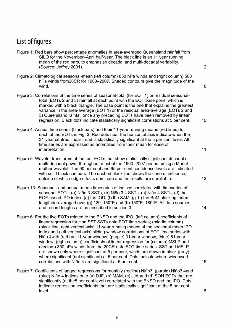
List of figures Figure 1: Red bars show percentage anomalies in area-averaged Queensland rainfall from

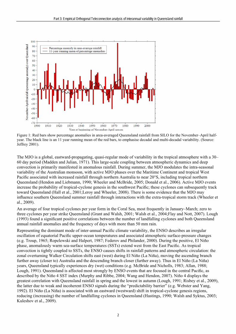
SILO for the November–April half-year. The black line is an 11 year running mean of the red bars, to emphasise decadal and multi-decadal variability. (Source: Jeffrey 2001). 2

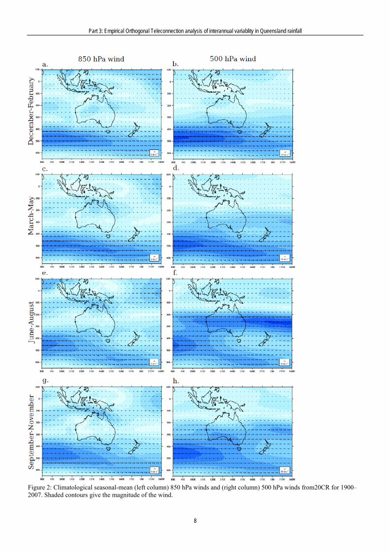
Figure 2: Climatological seasonal-mean (left column) 850 hPa winds and (right column) 500 hPa winds from20CR for 1900–2007. Shaded contours give the magnitude of the wind. 8

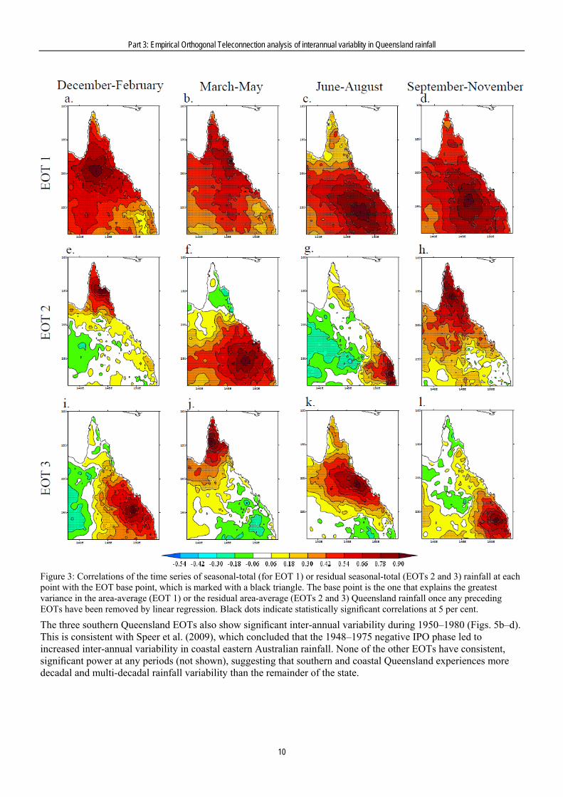
Figure 3: Correlations of the time series of seasonal-total (for EOT 1) or residual seasonal-total (EOTs 2 and 3) rainfall at each point with the EOT base point, which is marked with a black triangle. The base point is the one that explains the greatest variance in the area-average (EOT 1) or the residual area-average (EOTs 2 and 3) Queensland rainfall once any preceding EOTs have been removed by linear regression. Black dots indicate statistically significant correlations at 5 per cent. 10

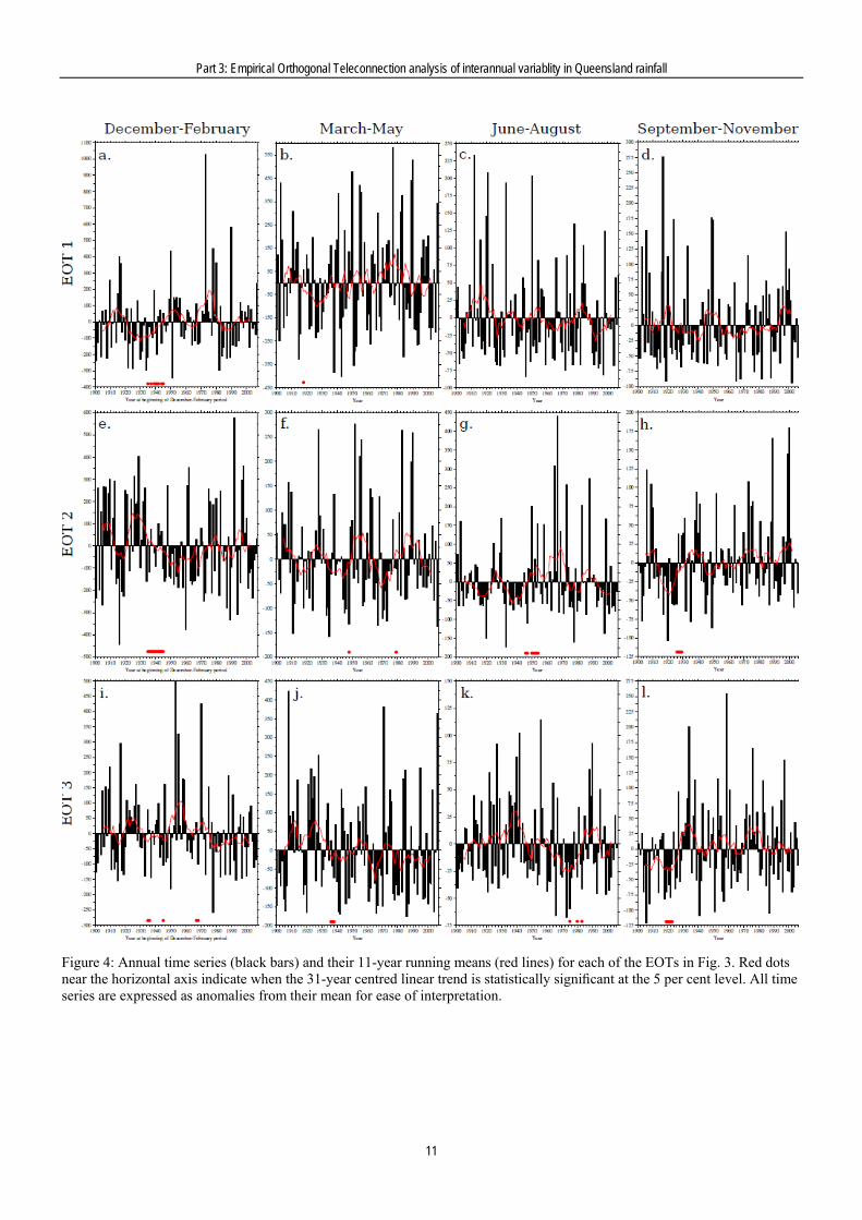
Figure 4: Annual time series (black bars) and their 11-year running means (red lines) for each of the EOTs in Fig. 3. Red dots near the horizontal axis indicate when the 31-year centred linear trend is statistically significant at the 5 per cent level. All time series are expressed as anomalies from their mean for ease of interpretation. 11

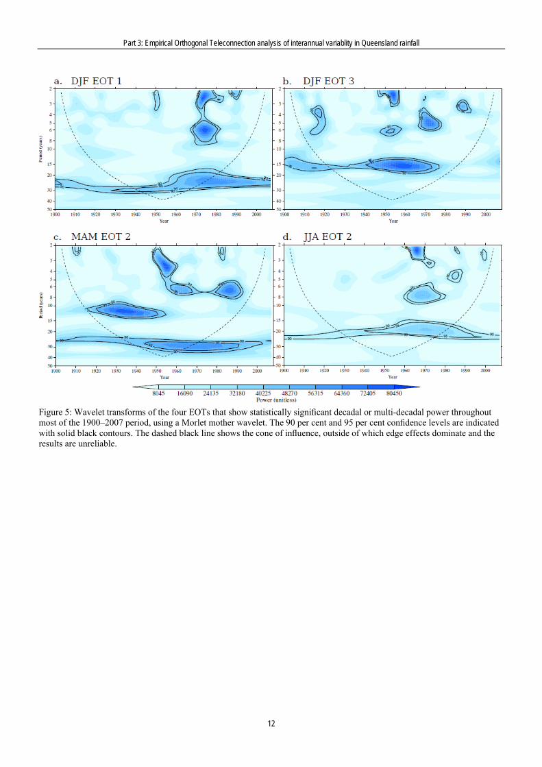
Figure 5: Wavelet transforms of the four EOTs that show statistically significant decadal or multi-decadal power throughout most of the 1900–2007 period, using a Morlet mother wavelet. The 90 per cent and 95 per cent confidence levels are indicated with solid black contours. The dashed black line shows the cone of influence, outside of which edge effects dominate and the results are unreliable. 12

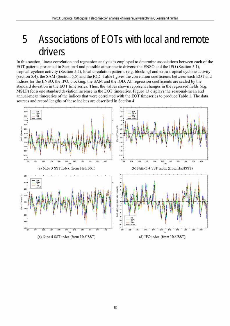
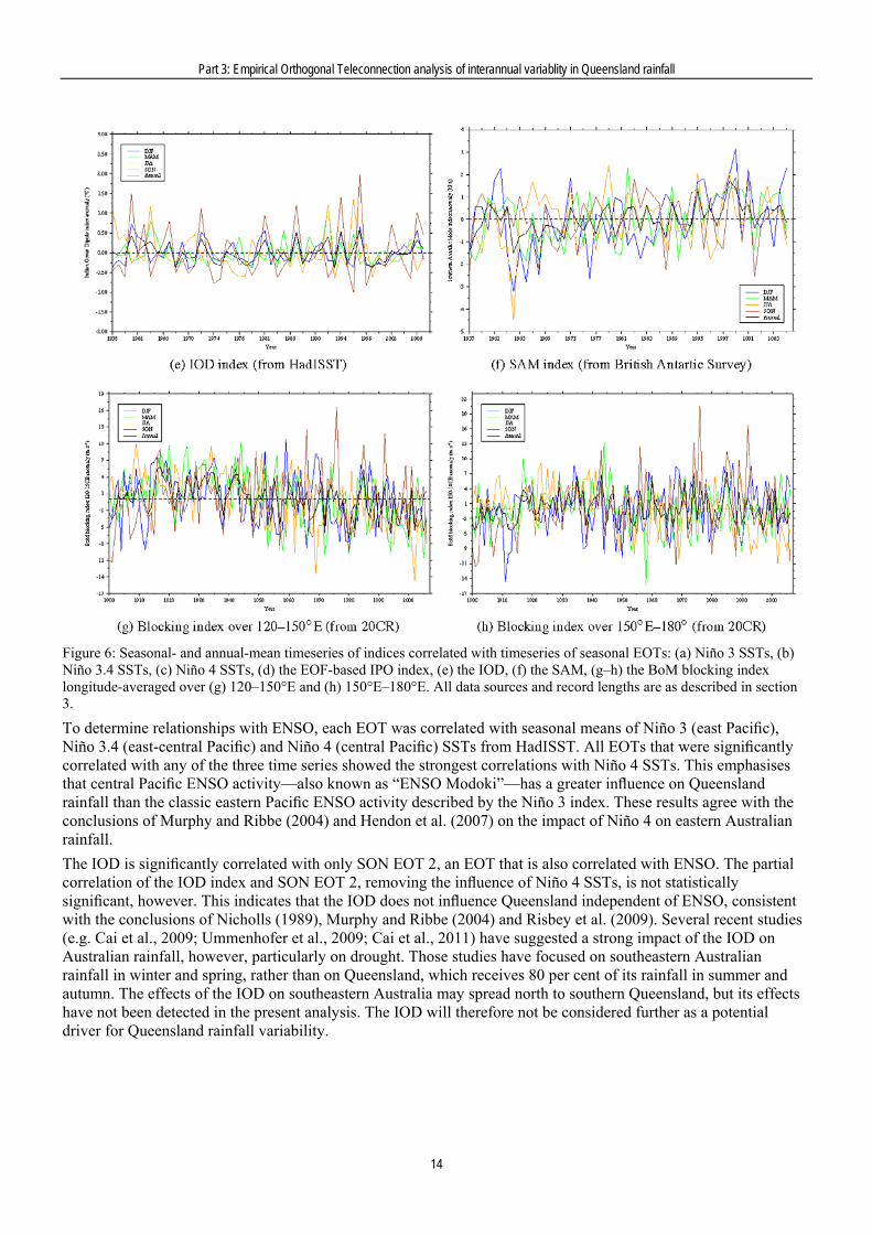
Figure 13: Seasonal- and annual-mean timeseries of indices correlated with timeseries of seasonal EOTs: (a) Niño 3 SSTs, (b) Niño 3.4 SSTs, (c) Niño 4 SSTs, (d) the EOF-based IPO index, (e) the IOD, (f) the SAM, (g–h) the BoM blocking index longitude-averaged over (g) 120–150°E and (h) 150°E–180°E. All data sources and record lengths are as described in section 3. 14

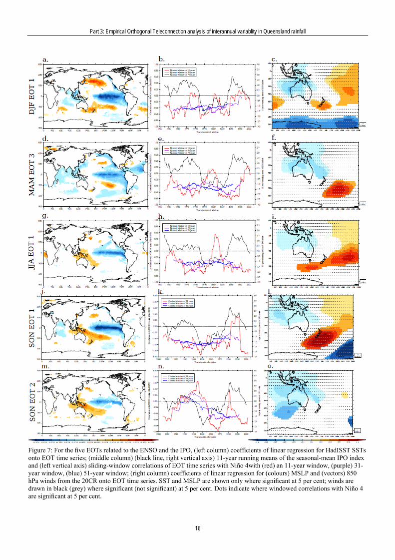
Figure 6: For the five EOTs related to the ENSO and the IPO, (left column) coefficients of linear regression for HadISST SSTs onto EOT time series; (middle column) (black line, right vertical axis) 11-year running means of the seasonal-mean IPO index and (left vertical axis) sliding-window correlations of EOT time series with Niño 4with (red) an 11-year window, (purple) 31-year window, (blue) 51-year window; (right column) coefficients of linear regression for (colours) MSLP and (vectors) 850 hPa winds from the 20CR onto EOT time series. SST and MSLP are shown only where significant at 5 per cent; winds are drawn in black (grey) where significant (not significant) at 5 per cent. Dots indicate where windowed correlations with Niño 4 are significant at 5 per cent. 16

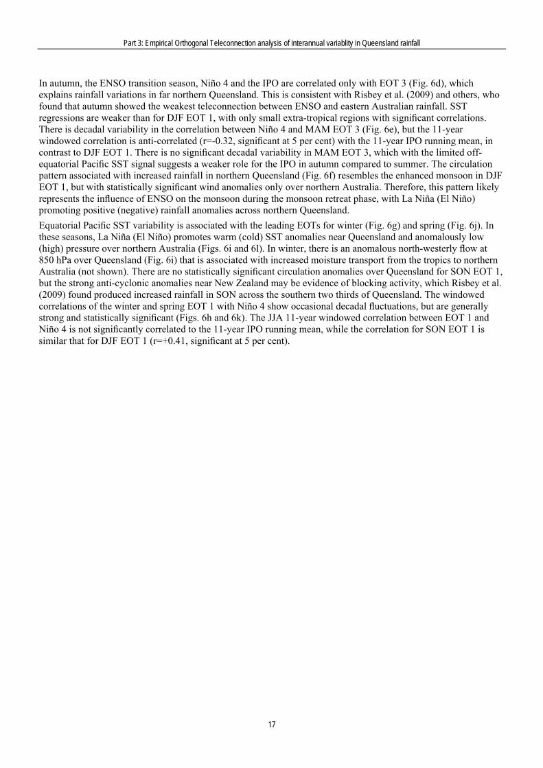
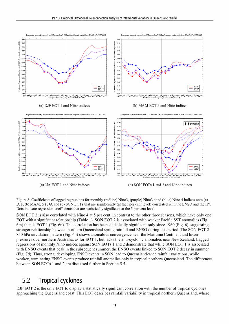
Figure 7: Coefficients of lagged regressions for monthly (redline) Niño3, (purple) Niño3.4and (blue) Niño 4 indices onto (a) DJF, (b) MAM, (c) JJA and (d) SON EOTs that are significantly (at the5 per cent level) correlated with the ENSO and the IPO. Dots indicate regression coefficients that are statistically significant at the 5 per cent level. 18

iii

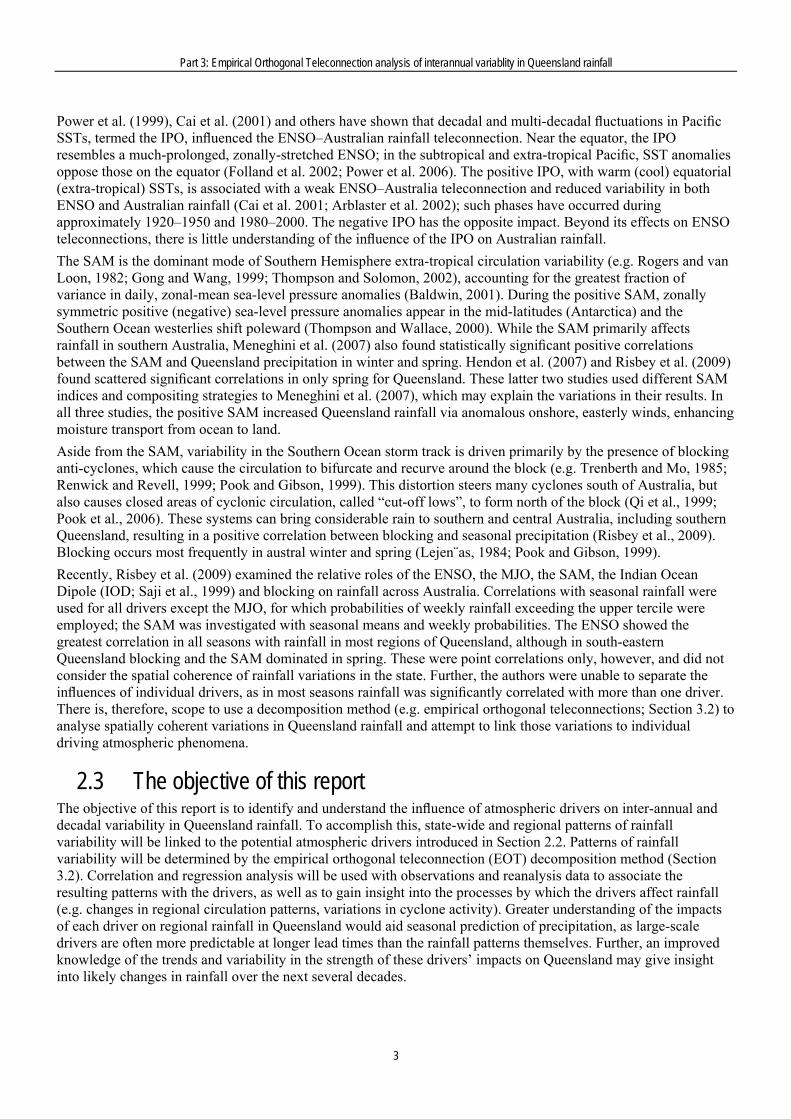
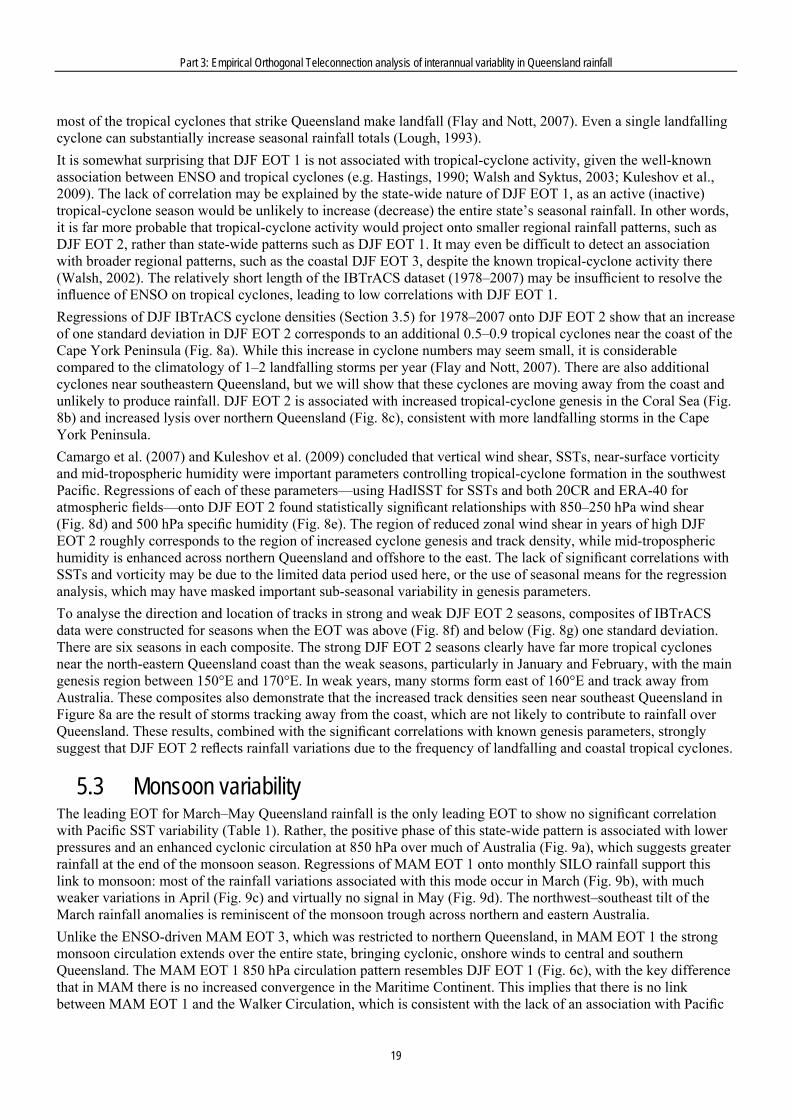
Figure 8: (a-c) Coefficients of linear regression of IBTrACS DJF tropical-cyclone (a) track density, (b) genesis density and (c) lysis density onto the DJF EOT 2 time series for 1978–2007; (d–e) coefficients of linear regression of (d) DJF 850–250 hPa zonal wind shear and (e) DJF 500 hPa winds and specific humidity from 20CR onto the DJF EOT 2 time series for 1900–2007; (f–g) DJF tropical-cyclone tracks from IBTrACS for the six seasons in 1978–2007 when DJF EOT 2 is (f) greater than and (g) less than one standard deviation. In (a–e), regression coefficients for all fields except 500 hPa winds are shown only where statistically significant at the 5 per cent level; 500 hPa winds are drawn in black (grey) where significant (not significant) at 5 per cent. Units of (a–c) are storms season−1 within a 5° spherical cap at each grid point. In (f–g), tracks are coloured by the month in which the cyclone forms; a circle (triangle) indicates the genesis (lysis) location. 20

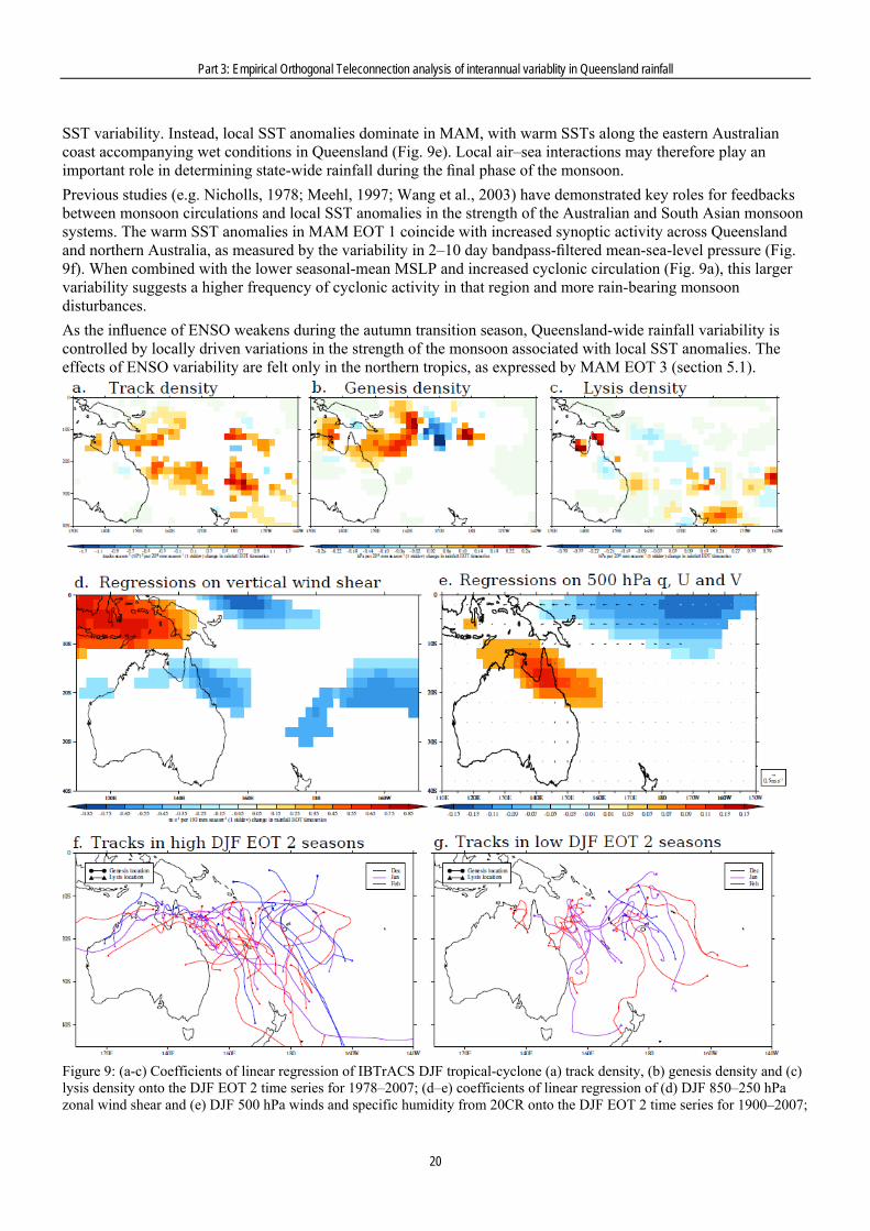
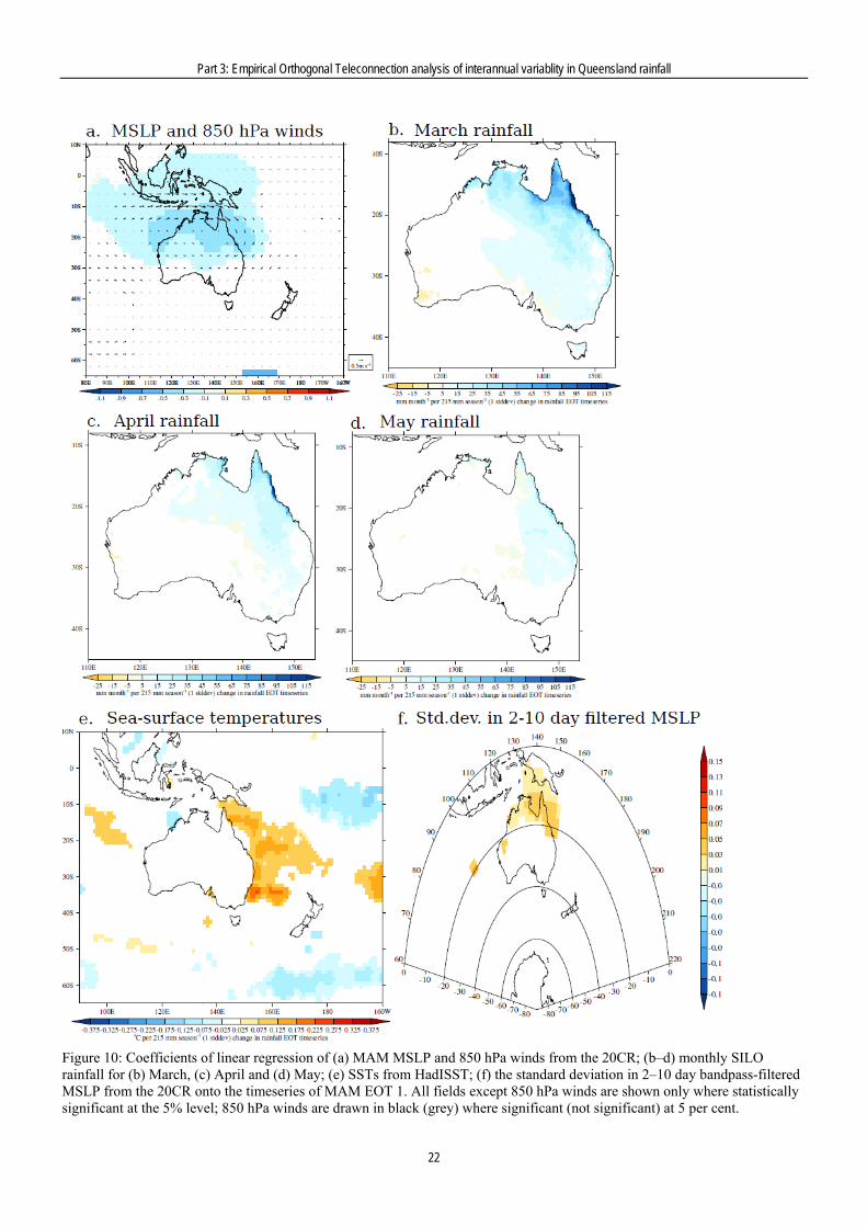
Figure 9: Coefficients of linear regression of (a) MAM MSLP and 850 hPa winds from the 20CR; (b–d) monthly SILO rainfall for (b) March, (c) April and (d) May; (e) SSTs from HadISST; (f) the standard deviation in 2–10 day bandpass-filtered MSLP from the 20CR onto the timeseries of MAM EOT 1. All fields except 850 hPa winds are shown only where statistically significant at the 5% level; 850 hPa winds are drawn in black (grey) where significant (not significant) at 5 per cent. 22

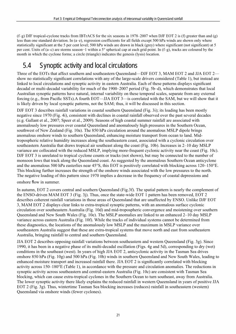
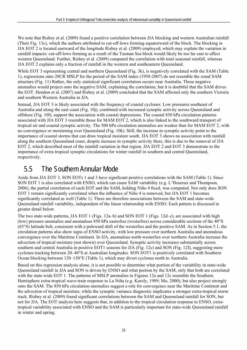
Figure 10: For the four EOTs related to local circulation pattern, the coefficients of linear regression of (left column) seasonal-mean MSLP (contours) and 850 hPa winds (vectors) from the 20CR; (centre column) seasonal-mean 500 hPa specific humidity (contours) and 500 hPa winds (vectors) from the 20CR; (right column) the standard deviation of 2-10 bandpass-filtered MSLP from the 20CR onto the timeseries of each EOT. All fields except the winds are shown only where statistical significance at the 5% level; wind vectors are drawn in black (grey) where significant (not significant) at the 5 per cent level. 24

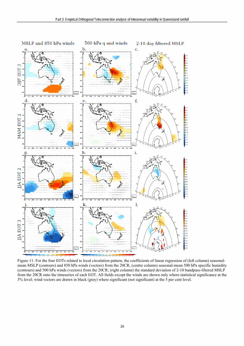
Figure 11: Coefficients of linear regression of seasonal-mean MSLP from the 20CR onto timeseries of JJA EOT 3. The data period is 1958-2007, for consistency with the SAM index. 25

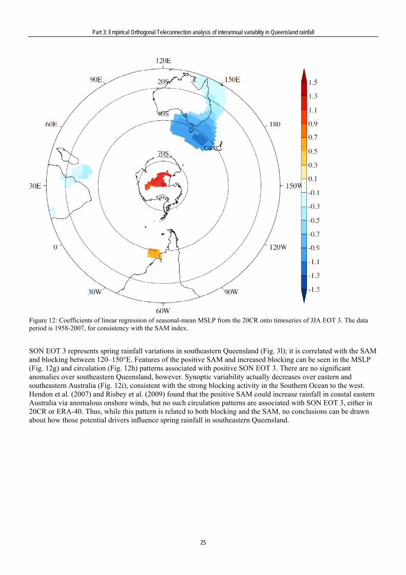
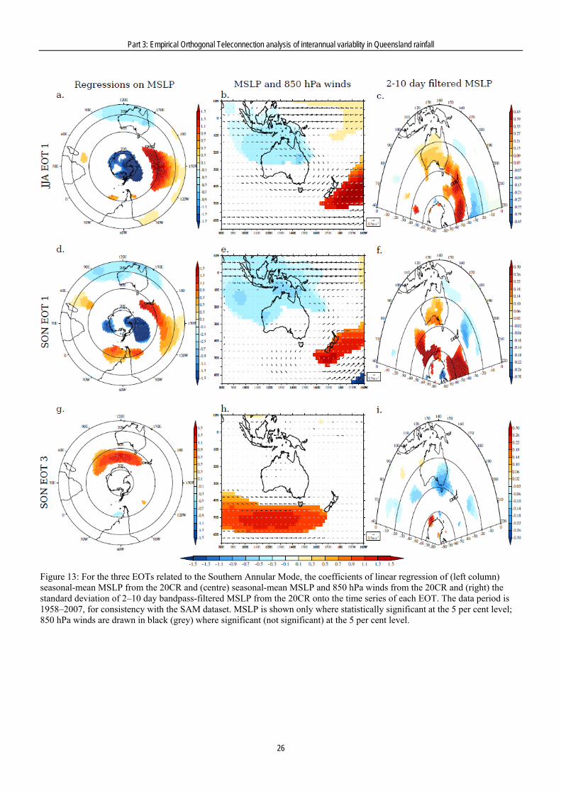
Figure 12: For the three EOTs related to the Southern Annular Mode, the coefficients of linear regression of (left column) seasonal-mean MSLP from the 20CR and (centre) seasonal-mean MSLP and 850 hPa winds from the 20CR and (right) the standard deviation of 2–10 day bandpass-filtered MSLP from the 20CR onto the time series of each EOT. The data period is 1958–2007, for consistency with the SAM dataset. MSLP is shown only where statistically significant at the 5 per cent level; 850 hPa winds are drawn in black (grey) where significant (not significant) at the 5 per cent level. 26

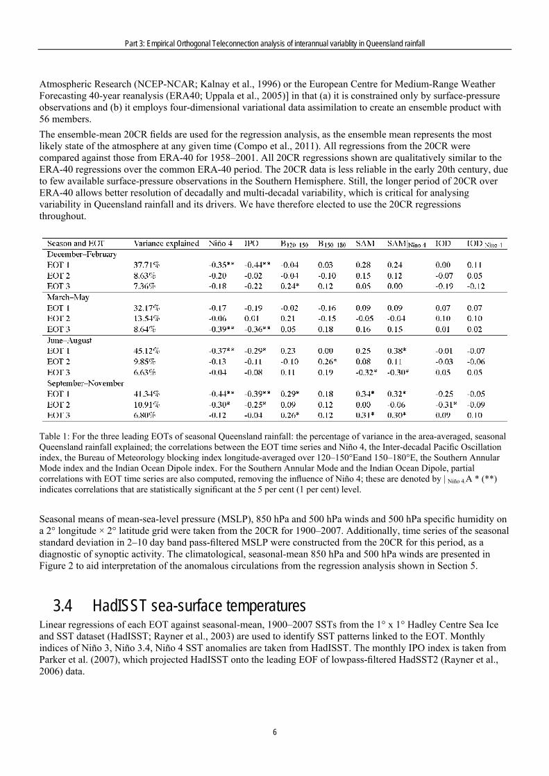
List of tables Table 1: For the three leading EOTs of seasonal Queensland rainfall: the percentage of

variance in the area-averaged, seasonal Queensland rainfall explained; the correlations between the EOT time series and Niño 4, the Inter-decadal Pacific Oscillation index, the Bureau of Meteorology blocking index longitude-averaged over 120–150°Eand 150–180°E, the Southern Annular Mode index and the Indian Ocean Dipole index. For the Southern Annular Mode and the Indian Ocean Dipole, partial correlations with EOT time series are also computed, removing the influence of Niño 4; these are denoted by | Niño 4.A * (**) indicates correlations that are statistically significant at the 5 per cent (1 per cent) level. 6

iv

Table 2 Summary of EOT analysis, giving percentage of variance explained in Queensland-average rainfall, the region of Queensland encompassed by the pattern, and the likely driving mechanism for each EOT. 27

v

Part 3: Empirical Orthogonal Teleconnection analysis of interannual variablity in Queensland rainfall

Executive Summary Climate drivers are more predictable than the rainfall patterns themselves and as such it is important to identify and understand the influence of climate drivers on inter-annual and decadal variations in Queensland rainfall. Identifying these climate drivers in historical records would provide a baseline against which to evaluate the climate model simulations of these drivers and Queensland rainfall. In addition understanding of the climate driver/rainfall relationship would greatly improve seasonal rainfall prediction. Empirical orthogonal teleconnection (EOT) analysis is applied to the 1900-2008 gridded SILO rainfall dataset to determine the climate drivers of seasonal rainfall in Queensland. EOT analysis identifies coherent spatial patterns of rainfall variability in the historical dataset, allowing the identification of climate drivers of specific regional rainfall variations. Most of the published work to date has not been able to identify the influence of each individual driver on Queensland rainfall as most rainfall seasons were significantly correlated with more than one driver. It is therefore necessary to decompose spatially coherent variations in Queensland rainfall and link these variations to individual driving atmospheric phenomena. To achieve this a combination of ERA-40, the new ECMWF Interim Reanalyses and other observational datasets, particularly those developed in Queensland and by the Met Office Hadley Centre, to investigate the processes and phenomena associated with the behaviour of Queensland rainfall over the last few decades were used.

2 Introduction 2.1 Inter-annual and decadal variability in Queensland’s rainfall

The state of Queensland, in north-eastern Australia, has experienced considerable inter-annual and decadal variability in its rainfall since reliable observations began in the late nineteenth century (e.g. Lough, 1991; Lavery et al., 1997; Hennessy et al., 1999). A time series of area-averaged Queensland rainfall from SILO (Section 3.1; Jeffrey, 2001) for November–April, during which Queensland receives 80 per cent of its annual rain, shows sustained periods of flood (e.g. 1950–1958, 1971–1978) and drought (e.g. 1929–1935, 1981–1988) years (Fig. 1). This variability is much larger than the linear trends in seasonal or annual rainfall (Nicholls and Lavery, 1992), which are small and statistically insignificant for the state as a whole (Lough, 1997). Coastal Queensland rainfall has declined since the 1950s, consistent with the rest of eastern Australia (Gallant et al., 2007; Alexander et al., 2007), but it is unclear whether this decline represents a forced shift in the long-term mean rainfall (i.e. from anthropogenic climate change) or the negative phase of a natural, multi-decadal or centennial oscillation (Cai et al., 2010). Understanding and predicting Queensland’s inter-annual rainfall variability is critical for mitigating the impacts of that variability on agriculture, hydrology and infrastructure.

2.2 Drivers of Queensland rainfall variability Variability in Queensland’s rainfall has been linked to local and remote atmospheric phenomena, including the Madden–Julian Oscillation (MJO) (e.g. Hendon and Liebmann,1990; Robertson et al., 2006; Wheeler et al., 2009), tropical cyclones (e.g. Lough, 1993; Walsh and Syktus, 2003; Flay and Nott, 2007), variability in extra-tropical storm tracks due to blocking in the Southern Ocean (e.g. Pook and Gibson, 1999; Risbey et al., 2008) and intense coastal cyclones (e.g. Holland, 1997), the El Niño–Southern Oscillation (ENSO) (e.g. Allan, 1988; Wang and Hendon, 2007), the Inter-Decadal Pacific Oscillation (IPO) (e.g. Power et al., 1999) and the Southern Annular Mode (SAM) (e.g. Meneghini et al., 2007; Hendon et al., 2007). The impacts of these drivers will be examined briefly in this section.

1

1


Figure 1: Red bars show percentage anomalies in area-averaged Queensland rainfall from SILO for the November–April half-year. The black line is an 11 year running mean of the red bars, to emphasise decadal and multi-decadal variability. (Source: Jeffrey 2001). The MJO is a global, eastward-propagating, quasi-regular mode of variability in the tropical atmosphere with a 30–60 day period (Madden and Julian, 1971). This large-scale coupling between atmospheric dynamics and deep convection is primarily manifested in anomalous rainfall. During summer, the MJO modulates the intra-seasonal variability of the Australian monsoon, with active MJO phases over the Maritime Continent and tropical West Pacific associated with increased rainfall through northern Australia to near 20°S, including tropical northern Queensland (Hendon and Liebmann, 1990; Wheeler and McBride, 2005; Donald et al., 2006). Active MJO events increase the probability of tropical-cyclone genesis in the southwest Pacific; these cyclones can subsequently track toward Queensland (Hall et al., 2001;Leroy and Wheeler, 2008). There is some evidence that the MJO may influence southern Queensland summer rainfall through interactions with the extra-tropical storm track (Wheeler et al., 2009). An average of four tropical cyclones per year form in the Coral Sea, most frequently in January–March; zero to three cyclones per year strike Queensland (Grant and Walsh, 2001; Walsh et al., 2004;Flay and Nott, 2007). Lough (1993) found a significant positive correlations between the number of landfalling cyclones and both Queensland annual rainfall anomalies and the frequency of days with more than 50 mm rain. Representing the dominant mode of inter-annual Pacific climate variability, the ENSO describes an irregular oscillation of equatorial Pacific upper-ocean temperatures and associated atmospheric surface-pressure changes (e.g. Troup, 1965; Ropelewski and Halpert, 1987; Federov and Philander, 2000). During the positive, El Niño phase, anomalously warm sea-surface temperatures (SSTs) extend west from the East Pacific. As tropical convection is tightly coupled to SSTs, the ENSO causes shifts in rainfall patterns and atmospheric circulation: the zonal overturning Walker Circulation shifts east (west) during El Niño (La Niña), moving the ascending branch further away (closer to) Australia and the descending branch closer (further away). Thus in El Niño (La Niña) years, Queensland typically experiences dry (wet) conditions (e.g. McBride and Nicholls, 1983; Allan, 1988; Lough, 1991). Queensland is affected most strongly by ENSO events that are focused in the central Pacific, as described by the Niño 4 SST index (Murphy and Ribbe, 2004; Wang and Hendon, 2007). Niño 4 displays the greatest correlation with Queensland rainfall in spring and the lowest in autumn (Lough, 1991; Risbey et al., 2009), the latter due to weak and incoherent ENSO signals during the “predictability barrier” (e.g. Webster and Yang, 1992). El Niño (La Niña) is associated with an eastward (westward) shift in tropical-cyclone genesis regions, reducing (increasing) the number of landfalling cyclones in Queensland (Hastings, 1990; Walsh and Syktus, 2003; Kuleshov et al., 2009).

2


Power et al. (1999), Cai et al. (2001) and others have shown that decadal and multi-decadal fluctuations in Pacific SSTs, termed the IPO, influenced the ENSO–Australian rainfall teleconnection. Near the equator, the IPO resembles a much-prolonged, zonally-stretched ENSO; in the subtropical and extra-tropical Pacific, SST anomalies oppose those on the equator (Folland et al. 2002; Power et al. 2006). The positive IPO, with warm (cool) equatorial (extra-tropical) SSTs, is associated with a weak ENSO–Australia teleconnection and reduced variability in both ENSO and Australian rainfall (Cai et al. 2001; Arblaster et al. 2002); such phases have occurred during approximately 1920–1950 and 1980–2000. The negative IPO has the opposite impact. Beyond its effects on ENSO teleconnections, there is little understanding of the influence of the IPO on Australian rainfall. The SAM is the dominant mode of Southern Hemisphere extra-tropical circulation variability (e.g. Rogers and van Loon, 1982; Gong and Wang, 1999; Thompson and Solomon, 2002), accounting for the greatest fraction of variance in daily, zonal-mean sea-level pressure anomalies (Baldwin, 2001). During the positive SAM, zonally symmetric positive (negative) sea-level pressure anomalies appear in the mid-latitudes (Antarctica) and the Southern Ocean westerlies shift poleward (Thompson and Wallace, 2000). While the SAM primarily affects rainfall in southern Australia, Meneghini et al. (2007) also found statistically significant positive correlations between the SAM and Queensland precipitation in winter and spring. Hendon et al. (2007) and Risbey et al. (2009) found scattered significant correlations in only spring for Queensland. These latter two studies used different SAM indices and compositing strategies to Meneghini et al. (2007), which may explain the variations in their results. In all three studies, the positive SAM increased Queensland rainfall via anomalous onshore, easterly winds, enhancing moisture transport from ocean to land. Aside from the SAM, variability in the Southern Ocean storm track is driven primarily by the presence of blocking anti-cyclones, which cause the circulation to bifurcate and recurve around the block (e.g. Trenberth and Mo, 1985; Renwick and Revell, 1999; Pook and Gibson, 1999). This distortion steers many cyclones south of Australia, but also causes closed areas of cyclonic circulation, called “cut-off lows”, to form north of the block (Qi et al., 1999; Pook et al., 2006). These systems can bring considerable rain to southern and central Australia, including southern Queensland, resulting in a positive correlation between blocking and seasonal precipitation (Risbey et al., 2009). Blocking occurs most frequently in austral winter and spring (Lejen¨as, 1984; Pook and Gibson, 1999). Recently, Risbey et al. (2009) examined the relative roles of the ENSO, the MJO, the SAM, the Indian Ocean Dipole (IOD; Saji et al., 1999) and blocking on rainfall across Australia. Correlations with seasonal rainfall were used for all drivers except the MJO, for which probabilities of weekly rainfall exceeding the upper tercile were employed; the SAM was investigated with seasonal means and weekly probabilities. The ENSO showed the greatest correlation in all seasons with rainfall in most regions of Queensland, although in south-eastern Queensland blocking and the SAM dominated in spring. These were point correlations only, however, and did not consider the spatial coherence of rainfall variations in the state. Further, the authors were unable to separate the influences of individual drivers, as in most seasons rainfall was significantly correlated with more than one driver. There is, therefore, scope to use a decomposition method (e.g. empirical orthogonal teleconnections; Section 3.2) to analyse spatially coherent variations in Queensland rainfall and attempt to link those variations to individual driving atmospheric phenomena.

2.3 The objective of this report The objective of this report is to identify and understand the influence of atmospheric drivers on inter-annual and decadal variability in Queensland rainfall. To accomplish this, state-wide and regional patterns of rainfall variability will be linked to the potential atmospheric drivers introduced in Section 2.2. Patterns of rainfall variability will be determined by the empirical orthogonal teleconnection (EOT) decomposition method (Section 3.2). Correlation and regression analysis will be used with observations and reanalysis data to associate the resulting patterns with the drivers, as well as to gain insight into the processes by which the drivers affect rainfall (e.g. changes in regional circulation patterns, variations in cyclone activity). Greater understanding of the impacts of each driver on regional rainfall in Queensland would aid seasonal prediction of precipitation, as large-scale drivers are often more predictable at longer lead times than the rainfall patterns themselves. Further, an improved knowledge of the trends and variability in the strength of these drivers’ impacts on Queensland may give insight into likely changes in rainfall over the next several decades.

3


The remainder of this report is organised as follows: the EOT technique and the datasets used for this study are described in Section 3; the leading three EOTs of seasonal Queensland rainfall are introduced and their temporal variability analysed in Section 4; associations between each EOT and atmospheric drivers are made in Section 5; the main conclusions of this report are discussed and summarised in Section 6.

4


3 Datasets and methods 3.1 SILO gridded rainfall analyses

Monthly and seasonal rainfall totals were taken from the SILO dataset of kriged gauge values on a 25 kilometre grid (Jeffrey, 2001). The SILO data were originally provided on a 5 kilometre grid, but were aggregated to 25 kilometres using an area-weighted linear interpolation method. The aggregation does not affect the EOT patterns; the EOTs computed from the 25 kilometre and 5 kilometre data are virtually identical. SILO data were available for 1890–2008; March 1900–February 2008 are analysed here, for a total of 108 years for each of the four seasons: December–February (DJF), March–May (MAM), June–August (JJA) and September–November (SON). Hereafter, seasons will be identified by the calendar year in which they begin (e.g. DJF 2007 is December 2007–February 2008); thus, the period of this study is 1900–2007. Very few rainfall stations in Queensland have records prior to 1900 (Lough, 1991; Lavery et al., 1997). Jeffrey (2001) used cross-validation to show that the monthly SILO totals were reliable across most of Queensland, with particular skill in coastal regions with high station densities, but were less skilful in the far north of the Cape York Peninsula where there are few stations with long records.

3.2 Empirical orthogonal teleconnection analysis EOT analysis decomposes a temporally and spatially varying field into a set of orthogonal patterns, called EOTs (Van Den Dool et al., 2001). Unlike patterns derived from empirical orthogonal function (EOF) analysis, which are orthogonal in both space and time, EOTs are orthogonal in either space or time only. This study employs EOTs that are orthogonal in time. Decomposition is achieved by first identifying the spatial point within the search domain that explains the greatest variance at all other points. The effect of the first point on all other points is then removed by linear regression, before identifying the point that explains the most variance in the residual field. The technique is repeated until the desired number of patterns are found. Van Den Dool et al. (2001) demonstrated that EOTs of three commonly used climate fields—surface temperatures, soil moisture and geopotential heights—strongly resembled rotated EOFs, but the EOTs were computed much more efficiently. In an analysis of Australian rainfall, Smith (2004) argued for an EOT procedure in which patterns were identified by the explained variance in area-averaged Australian rainfall, rather than by total space–time variance explained at all points as in Van Den Dool et al. (2001). This is a particular issue for Australia, where most of the rainfall, and hence most of the variance, is concentrated along the coast. Rotstayn et al. (2010) employed the Smith (2004) procedure to analyse improvements in the CSIRO Mk 3.6 model’s simulation of inter-annual variability of Australian rainfall. EOTs were computed for each three-month season using seasonal-total 1900–2007 SILO rainfall over a domain approximating Queensland: 9–30°S, 138–154°E. Initially, the EOTs were identified using three methods: the covariance-based method of Van Den Dool et al. (2001), a correlation-based method using standardised rainfall anomalies also described in Van Den Dool et al. (2001), and the area-average method of Smith (2004). The covariance method differed from the other two in that patterns were shifted towards the coast, as suggested by Smith (2004). The correlation and area-averaged methods produced similar EOTs, both in the spatial patterns and in the amount of variance explained. Only the patterns using the Smith (2004) method will be examined further here. The first three EOTs are analysed for each season, as together these patterns explain at least 53 per cent of the variance in the Queensland-average rainfall timeseries in all seasons (Table 1). Subsequent EOTs each explain less than 5 per cent variance.

3.3 Reanalysis data To analyse the atmospheric circulation patterns associated with each EOT, the EOT time series are linearly regressed against fields from the 20th Century Reanalysis (20CR; Compo et al., 2011) for 1900–2007. The 20CR differs from other reanalyses [e.g. the National Centres for Environmental Prediction–National Centre for

5


Atmospheric Research (NCEP-NCAR; Kalnay et al., 1996) or the European Centre for Medium-Range Weather Forecasting 40-year reanalysis (ERA40; Uppala et al., 2005)] in that (a) it is constrained only by surface-pressure observations and (b) it employs four-dimensional variational data assimilation to create an ensemble product with 56 members. The ensemble-mean 20CR fields are used for the regression analysis, as the ensemble mean represents the most likely state of the atmosphere at any given time (Compo et al., 2011). All regressions from the 20CR were compared against those from ERA-40 for 1958–2001. All 20CR regressions shown are qualitatively similar to the ERA-40 regressions over the common ERA-40 period. The 20CR data is less reliable in the early 20th century, due to few available surface-pressure observations in the Southern Hemisphere. Still, the longer period of 20CR over ERA-40 allows better resolution of decadally and multi-decadal variability, which is critical for analysing variability in Queensland rainfall and its drivers. We have therefore elected to use the 20CR regressions throughout.

Table 1: For the three leading EOTs of seasonal Queensland rainfall: the percentage of variance in the area-averaged, seasonal Queensland rainfall explained; the correlations between the EOT time series and Niño 4, the Inter-decadal Pacific Oscillation index, the Bureau of Meteorology blocking index longitude-averaged over 120–150°Eand 150–180°E, the Southern Annular Mode index and the Indian Ocean Dipole index. For the Southern Annular Mode and the Indian Ocean Dipole, partial correlations with EOT time series are also computed, removing the influence of Niño 4; these are denoted by | Niño 4.A * (**) indicates correlations that are statistically significant at the 5 per cent (1 per cent) level. Seasonal means of mean-sea-level pressure (MSLP), 850 hPa and 500 hPa winds and 500 hPa specific humidity on a 2° longitude × 2° latitude grid were taken from the 20CR for 1900–2007. Additionally, time series of the seasonal standard deviation in 2–10 day band pass-filtered MSLP were constructed from the 20CR for this period, as a diagnostic of synoptic activity. The climatological, seasonal-mean 850 hPa and 500 hPa winds are presented in Figure 2 to aid interpretation of the anomalous circulations from the regression analysis shown in Section 5.

3.4 HadISST sea-surface temperatures Linear regressions of each EOT against seasonal-mean, 1900–2007 SSTs from the 1° x 1° Hadley Centre Sea Ice and SST dataset (HadISST; Rayner et al., 2003) are used to identify SST patterns linked to the EOT. Monthly indices of Niño 3, Niño 3.4, Niño 4 SST anomalies are taken from HadISST. The monthly IPO index is taken from Parker et al. (2007), which projected HadISST onto the leading EOF of lowpass-filtered HadSST2 (Rayner et al., 2006) data.

6


3.5 Tropical cyclone tracks Tropical cyclone tracks for the South Pacific basin were obtained from the International Best Track Archive for Climate Stewardship (IBTrACS Knapp et al., 2010). Due to limited observational coverage of South Pacific tropical cyclones prior to the satellite era, cyclone tracks were analysed for the period 1979–2007 only. To generate statistics of tropical cyclone activity such as track, genesis and lysis densities on a regular grid, each season of IBTrACS tracks were processed by the method of Hodges (1996). Track, genesis and lysis densities are expressed in units of storms per season within a 5 degree-radius spherical cap of each grid point; the unit area is approximately equal to 106 kilometre squared. As the South Pacific tropical-cyclone season runs from October–May, tracking statistics were obtained for SON, DJF and MAM seasons for correlation with the seasonal rainfall EOTs.

3.6 Blocking index To evaluate links between rainfall EOTs and blocking, we compute the Bureau of Meteorology blocking index (Pook and Gibson, 1999) from the 20CR monthly-mean 500 hPa zonal winds. The index identifies splits in the mid-tropospheric jet, which are associated with blocking anticyclones. At every longitude, the blocking index is defined as B =0.5(U25 +U30 − U40 − 2U45 − U50 +U55 +U60 ) (1) Seasonal means of the blocking index were computed from the monthly values. These seasonal means were then longitude averaged over two bands in the Southern Ocean—120-150°E and 150–180°E—where blocking activity has previously been shown to influence Australian rainfall (e.g. Qi et al., 1999; Pook et al., 2006; Risbey et al., 2008, 2009).

3.7 Southern Annular Mode index For correlations between rainfall EOTs and the SAM, we use the station-pressure index of Marshall (2003), computed as the difference between normalised monthly-mean, zonal-mean sea-level pressures at 40°S minus those at 65°S (Gong and Wang, 1999). Seasonal means of the SAM index were obtained for 1958–2007.

3.8 Indian Ocean Dipole index Correlations between rainfall EOTs and the Indian Ocean Dipole are calculated using the dipole mode index of Saji et al. (1999), defined as the difference in SST anomalies between two Indian Ocean boxes: 10°S–10°N, 50–70°E and 10°S–0°, 90–110°E. Seasonal means of the IOD index were computed from HadISST for 1900–2007.

7


Figure 2: Climatological seasonal-mean (left column) 850 hPa winds and (right column) 500 hPa winds from20CR for 1900–2007. Shaded contours give the magnitude of the wind.

8


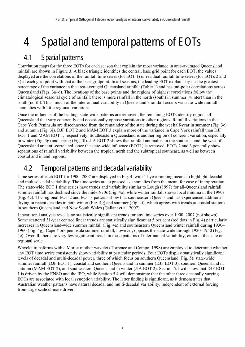
4 Spatial and temporal patterns of EOTs 4.1 Spatial patterns

Correlation maps for the three EOTs for each season that explain the most variance in area-averaged Queensland rainfall are shown in Figure 3. A black triangle identifies the central, base grid point for each EOT; the values displayed are the correlations of the rainfall time series (for EOT 1) or residual rainfall time series (for EOTs 2 and 3) at each grid point with that at the base gridpoint. In all seasons, the leading EOT explains by far the greatest percentage of the variance in the area-averaged Queensland rainfall (Table 1) and has uni-polar correlations across Queensland (Figs. 3a–d). The locations of the base points and the regions of highest correlations follow the climatological seasonal cycle of rainfall: there is more rainfall in the north (south) in summer (winter) than in the south (north). Thus, much of the inter-annual variability in Queensland’s rainfall occurs via state-wide rainfall anomalies with little regional variation. Once the influence of the leading, state-wide patterns are removed, the remaining EOTs identify regions of Queensland that vary coherently and occasionally oppose variations in other regions. Rainfall variations in the Cape York Peninsula are disconnected from the remainder of the state during the wet half-year in summer (Fig. 3e) and autumn (Fig. 3j). DJF EOT 2 and MAM EOT 3 explain more of the variance in Cape York rainfall than DJF EOT 1 and MAM EOT 1, respectively. Southeastern Queensland is another region of coherent variation, especially in winter (Fig. 3g) and spring (Fig. 3l). JJA EOT 2 shows that rainfall anomalies in the southeast and the west of Queensland are anti-correlated, once the state-wide influence (EOT1) is removed. EOTs 2 and 3 generally show separations of rainfall variability between the tropical north and the subtropical southeast, as well as between coastal and inland regions.

4.2 Temporal patterns and decadal variability Time series of each EOT for 1900–2007 are displayed in Fig. 4, with 11 year running means to highlight decadal and multi-decadal variability. The time series are expressed as anomalies from the mean, for ease of interpretation. The state-wide EOT 1 time series have trends and variability similar to Lough (1997) for all-Queensland rainfall: summer rainfall has declined since the mid-1970s (Fig. 4a), while winter rainfall shows local minima in the 1990s (Fig. 4c). The regional EOT 2 and EOT 3 patterns show that southeastern Queensland has experienced additional drying in recent decades in both winter (Fig. 4g) and summer (Fig. 4i), which agrees with trends at coastal stations in southern Queensland and New South Wales (Gallant et al. 2007). Linear trend analysis reveals no statistically significant trends for any time series over 1900–2007 (not shown). Some scattered 31-year centred linear trends are statistically significant at 5 per cent (red dots in Fig. 4) particularly increases in Queensland-wide summer rainfall (Fig. 4a) and southeastern Queensland winter rainfall during 1930–1960 (Fig. 4g). Cape York peninsula summer rainfall, however, opposes the state-wide through 1920–1950 (Fig. 4e). Overall, there are very few significant trends in these patterns of inter-annual variability, either at the state or regional scale. Wavelet transforms with a Morlet mother wavelet (Torrence and Compo, 1998) are employed to determine whether any EOT time series consistently show variability at particular periods. Four EOTs display statistically significant levels of decadal and multi-decadal power, three of which focus on southern Queensland (Fig. 5): state-wide summer rainfall (DJF EOT 1), coastal and southern Queensland in summer (DJF EOT 3), southern Queensland in autumn (MAM EOT 2), and southeastern Queensland in winter (JJA EOT 2). Section 5.1 will show that DJF EOT 1 is driven by the ENSO and the IPO, while Section 5.4 will demonstrate that the other three decanally varying EOTs are associated with local synoptic variability. The latter finding is significant, as it demonstrates that Australian weather patterns have natural decadal and multi-decadal variability, independent of external forcing from large-scale climate drivers.

9


Figure 3: Correlations of the time series of seasonal-total (for EOT 1) or residual seasonal-total (EOTs 2 and 3) rainfall at each point with the EOT base point, which is marked with a black triangle. The base point is the one that explains the greatest variance in the area-average (EOT 1) or the residual area-average (EOTs 2 and 3) Queensland rainfall once any preceding EOTs have been removed by linear regression. Black dots indicate statistically significant correlations at 5 per cent.

The three southern Queensland EOTs also show significant inter-annual variability during 1950–1980 (Figs. 5b–d). This is consistent with Speer et al. (2009), which concluded that the 1948–1975 negative IPO phase led to increased inter-annual variability in coastal eastern Australian rainfall. None of the other EOTs have consistent, significant power at any periods (not shown), suggesting that southern and coastal Queensland experiences more decadal and multi-decadal rainfall variability than the remainder of the state.

10


Figure 4: Annual time series (black bars) and their 11-year running means (red lines) for each of the EOTs in Fig. 3. Red dots near the horizontal axis indicate when the 31-year centred linear trend is statistically significant at the 5 per cent level. All time series are expressed as anomalies from their mean for ease of interpretation.

11


Figure 5: Wavelet transforms of the four EOTs that show statistically significant decadal or multi-decadal power throughout most of the 1900–2007 period, using a Morlet mother wavelet. The 90 per cent and 95 per cent confidence levels are indicated with solid black contours. The dashed black line shows the cone of influence, outside of which edge effects dominate and the results are unreliable.

12


5 Associations of EOTs with local and remote drivers

In this section, linear correlation and regression analysis is employed to determine associations between each of the EOT patterns presented in Section 4 and possible atmospheric drivers: the ENSO and the IPO (Section 5.1), tropical-cyclone activity (Section 5.2), local circulation patterns (e.g. blocking) and extra-tropical cyclone activity (section 5.4), the SAM (Section 5.5) and the IOD. Table1 gives the correlation coefficients between each EOT and indices for the ENSO, the IPO, blocking, the SAM and the IOD. All regression coefficients are scaled by the standard deviation in the EOT time series. Thus, the values shown represent changes in the regressed fields (e.g. MSLP) for a one standard deviation increase in the EOT timeseries. Figure 13 displays the seasonal-mean and annual-mean timeseries of the indices that were correlated with the EOT timeseries to produce Table 1. The data sources and record lengths of these indices are described in Section 4.

13


Figure 6: Seasonal- and annual-mean timeseries of indices correlated with timeseries of seasonal EOTs: (a) Niño 3 SSTs, (b) Niño 3.4 SSTs, (c) Niño 4 SSTs, (d) the EOF-based IPO index, (e) the IOD, (f) the SAM, (g–h) the BoM blocking index longitude-averaged over (g) 120–150°E and (h) 150°E–180°E. All data sources and record lengths are as described in section 3.

To determine relationships with ENSO, each EOT was correlated with seasonal means of Niño 3 (east Pacific), Niño 3.4 (east-central Pacific) and Niño 4 (central Pacific) SSTs from HadISST. All EOTs that were significantly correlated with any of the three time series showed the strongest correlations with Niño 4 SSTs. This emphasises that central Pacific ENSO activity—also known as “ENSO Modoki”—has a greater influence on Queensland rainfall than the classic eastern Pacific ENSO activity described by the Niño 3 index. These results agree with the conclusions of Murphy and Ribbe (2004) and Hendon et al. (2007) on the impact of Niño 4 on eastern Australian rainfall. The IOD is significantly correlated with only SON EOT 2, an EOT that is also correlated with ENSO. The partial correlation of the IOD index and SON EOT 2, removing the influence of Niño 4 SSTs, is not statistically significant, however. This indicates that the IOD does not influence Queensland independent of ENSO, consistent with the conclusions of Nicholls (1989), Murphy and Ribbe (2004) and Risbey et al. (2009). Several recent studies (e.g. Cai et al., 2009; Ummenhofer et al., 2009; Cai et al., 2011) have suggested a strong impact of the IOD on Australian rainfall, however, particularly on drought. Those studies have focused on southeastern Australian rainfall in winter and spring, rather than on Queensland, which receives 80 per cent of its rainfall in summer and autumn. The effects of the IOD on southeastern Australia may spread north to southern Queensland, but its effects have not been detected in the present analysis. The IOD will therefore not be considered further as a potential driver for Queensland rainfall variability.

14


5.1 The El Nino–Southern Oscillation and the Inter-decadal Pacific Oscillation

Five of the EOT patterns—DJF EOT 1, MAM EOT 3, JJA EOT 1 and SON EOTs 1 and 2—show statistically significant correlations with Niño 4 SST anomalies and the IPO index at the 5 per cent level or above (Table 1). Regressions of HadISST SSTs against each EOT time series confirm the relationships between variability in rainfall and equatorial Pacific SSTs (Fig. 6, left column). Lag regressions of monthly Niño 3, 3.4, and 4 against each EOT demonstrate that DJF EOT 1 is related to ENSO events that peak in the same DJF season (Fig. 7a); JJA (Fig. 7c) and SON (Fig. 7d) patterns are related to ENSO events that peak in the following DJF; and MAM EOT 3 is related to the preceding summer’s ENSO (Fig. 7b). The lag regressions will be discussed further when the differences between SON EOTs 1 and 2 are considered. During the austral monsoon, state-wide rainfall anomalies are associated with both equatorial and off-equatorial Pacific SST variability (Fig. 6a). The spatial pattern of SST regression coefficients strongly resembles the negative (cool) phase of the IPO (e.g. Power et al., 1999). Indeed, DJF EOT 1 is more strongly correlated with the IPO than with Niño 4, although both correlations are statistically significant at 1 per cent. Combined with the statistically significant multi-decadal power in DJF EOT 1 (Fig. 5a), this argues that decadal and multi-decadal Pacific SST variability exerts a control on inter-annual and multi-decadal fluctuations in summer rainfall. The correlation between DJF EOT 1 and Niño 4 shows considerable decadal variability (Fig. 6b, red line), although over 31 year and 51 year periods the correlation magnitude is stable. Periods of a weak 11-year correlation coincide with warm phases of the IPO (White et al. 2004, e.g. 1930–1945; 1980–2000). Fig. 6b displays a clear association between the 11-year running-mean of the IPO (black line) and the 11-year correlation between rainfall and Niño 4, with periods of weak (strong) 11-year correlations corresponding to warm (cool) IPO phases. The two time series are correlated with a coefficient of 0.42, significant at 5 per cent. Years of positive DJF EOT 1 are associated with an intensified cyclonic monsoon circulation at 850 hPa over much of Australia, as well as anomalous convergence over the Maritime Continent that reflects a westward shift in the Walker Circulation (Fig. 6c). The positive phase of the SOI can also clearly be seen, reinforcing the association with the ENSO. Thus, DJF EOT 1 represents variations in the Australian summer monsoon that are linked not only to modes of inter-annual and inter-decadal Pacific SST variability, but to the interactions between those modes.

15


Figure 7: For the five EOTs related to the ENSO and the IPO, (left column) coefficients of linear regression for HadISST SSTs onto EOT time series; (middle column) (black line, right vertical axis) 11-year running means of the seasonal-mean IPO index and (left vertical axis) sliding-window correlations of EOT time series with Niño 4with (red) an 11-year window, (purple) 31-year window, (blue) 51-year window; (right column) coefficients of linear regression for (colours) MSLP and (vectors) 850 hPa winds from the 20CR onto EOT time series. SST and MSLP are shown only where significant at 5 per cent; winds are drawn in black (grey) where significant (not significant) at 5 per cent. Dots indicate where windowed correlations with Niño 4 are significant at 5 per cent.

16


In autumn, the ENSO transition season, Niño 4 and the IPO are correlated only with EOT 3 (Fig. 6d), which explains rainfall variations in far northern Queensland. This is consistent with Risbey et al. (2009) and others, who found that autumn showed the weakest teleconnection between ENSO and eastern Australian rainfall. SST regressions are weaker than for DJF EOT 1, with only small extra-tropical regions with significant correlations. There is decadal variability in the correlation between Niño 4 and MAM EOT 3 (Fig. 6e), but the 11-year windowed correlation is anti-correlated (r=-0.32, significant at 5 per cent) with the 11-year IPO running mean, in contrast to DJF EOT 1. There is no significant decadal variability in MAM EOT 3, which with the limited off-equatorial Pacific SST signal suggests a weaker role for the IPO in autumn compared to summer. The circulation pattern associated with increased rainfall in northern Queensland (Fig. 6f) resembles the enhanced monsoon in DJF EOT 1, but with statistically significant wind anomalies only over northern Australia. Therefore, this pattern likely represents the influence of ENSO on the monsoon during the monsoon retreat phase, with La Niña (El Niño) promoting positive (negative) rainfall anomalies across northern Queensland. Equatorial Pacific SST variability is associated with the leading EOTs for winter (Fig. 6g) and spring (Fig. 6j). In these seasons, La Niña (El Niño) promotes warm (cold) SST anomalies near Queensland and anomalously low (high) pressure over northern Australia (Figs. 6i and 6l). In winter, there is an anomalous north-westerly flow at 850 hPa over Queensland (Fig. 6i) that is associated with increased moisture transport from the tropics to northern Australia (not shown). There are no statistically significant circulation anomalies over Queensland for SON EOT 1, but the strong anti-cyclonic anomalies near New Zealand may be evidence of blocking activity, which Risbey et al. (2009) found produced increased rainfall in SON across the southern two thirds of Queensland. The windowed correlations of the winter and spring EOT 1 with Niño 4 show occasional decadal fluctuations, but are generally strong and statistically significant (Figs. 6h and 6k). The JJA 11-year windowed correlation between EOT 1 and Niño 4 is not significantly correlated to the 11-year IPO running mean, while the correlation for SON EOT 1 is similar that for DJF EOT 1 (r=+0.41, significant at 5 per cent).

17


Figure 8: Coefficients of lagged regressions for monthly (redline) Niño3, (purple) Niño3.4and (blue) Niño 4 indices onto (a) DJF, (b) MAM, (c) JJA and (d) SON EOTs that are significantly (at the5 per cent level) correlated with the ENSO and the IPO. Dots indicate regression coefficients that are statistically significant at the 5 per cent level.

SON EOT 2 is also correlated with Niño 4 at 5 per cent, in contrast to the other three seasons, which have only one EOT with a significant relationship (Table 1). SON EOT 2 is associated with weaker Pacific SST anomalies (Fig. 6m) than is EOT 1 (Fig. 6n). The correlation has been statistically significant only since 1960 (Fig. 6), suggesting a stronger relationship between northern Queensland spring rainfall and ENSO during this period. The SON EOT 2 850 hPa circulation pattern (Fig. 6o) shows anomalous convergence near the Maritime Continent and lower pressures over northern Australia, as for EOT 1, but lacks the anti-cyclonic anomalies near New Zealand. Lagged regressions of monthly Niño indices against SON EOTs 1 and 2 demonstrate that while SON EOT 1 is associated with ENSO events that peak in the subsequent summer, the ENSO events linked to SON EOT 2 decay in summer (Fig. 7d). Thus, strong, developing ENSO events in SON lead to Queensland-wide rainfall variations, while weaker, terminating ENSO events produce rainfall anomalies only in tropical northern Queensland. The differences between SON EOTs 1 and 2 are discussed further in Section 5.5.

5.2 Tropical cyclones DJF EOT 2 is the only EOT to display a statistically significant correlation with the number of tropical cyclones approaching the Queensland coast. This EOT describes rainfall variability in tropical northern Queensland, where

18


most of the tropical cyclones that strike Queensland make landfall (Flay and Nott, 2007). Even a single landfalling cyclone can substantially increase seasonal rainfall totals (Lough, 1993). It is somewhat surprising that DJF EOT 1 is not associated with tropical-cyclone activity, given the well-known association between ENSO and tropical cyclones (e.g. Hastings, 1990; Walsh and Syktus, 2003; Kuleshov et al., 2009). The lack of correlation may be explained by the state-wide nature of DJF EOT 1, as an active (inactive) tropical-cyclone season would be unlikely to increase (decrease) the entire state’s seasonal rainfall. In other words, it is far more probable that tropical-cyclone activity would project onto smaller regional rainfall patterns, such as DJF EOT 2, rather than state-wide patterns such as DJF EOT 1. It may even be difficult to detect an association with broader regional patterns, such as the coastal DJF EOT 3, despite the known tropical-cyclone activity there (Walsh, 2002). The relatively short length of the IBTrACS dataset (1978–2007) may be insufficient to resolve the influence of ENSO on tropical cyclones, leading to low correlations with DJF EOT 1. Regressions of DJF IBTrACS cyclone densities (Section 3.5) for 1978–2007 onto DJF EOT 2 show that an increase of one standard deviation in DJF EOT 2 corresponds to an additional 0.5–0.9 tropical cyclones near the coast of the Cape York Peninsula (Fig. 8a). While this increase in cyclone numbers may seem small, it is considerable compared to the climatology of 1–2 landfalling storms per year (Flay and Nott, 2007). There are also additional cyclones near southeastern Queensland, but we will show that these cyclones are moving away from the coast and unlikely to produce rainfall. DJF EOT 2 is associated with increased tropical-cyclone genesis in the Coral Sea (Fig. 8b) and increased lysis over northern Queensland (Fig. 8c), consistent with more landfalling storms in the Cape York Peninsula. Camargo et al. (2007) and Kuleshov et al. (2009) concluded that vertical wind shear, SSTs, near-surface vorticity and mid-tropospheric humidity were important parameters controlling tropical-cyclone formation in the southwest Pacific. Regressions of each of these parameters—using HadISST for SSTs and both 20CR and ERA-40 for atmospheric fields—onto DJF EOT 2 found statistically significant relationships with 850–250 hPa wind shear (Fig. 8d) and 500 hPa specific humidity (Fig. 8e). The region of reduced zonal wind shear in years of high DJF EOT 2 roughly corresponds to the region of increased cyclone genesis and track density, while mid-tropospheric humidity is enhanced across northern Queensland and offshore to the east. The lack of significant correlations with SSTs and vorticity may be due to the limited data period used here, or the use of seasonal means for the regression analysis, which may have masked important sub-seasonal variability in genesis parameters. To analyse the direction and location of tracks in strong and weak DJF EOT 2 seasons, composites of IBTrACS data were constructed for seasons when the EOT was above (Fig. 8f) and below (Fig. 8g) one standard deviation. There are six seasons in each composite. The strong DJF EOT 2 seasons clearly have far more tropical cyclones near the north-eastern Queensland coast than the weak seasons, particularly in January and February, with the main genesis region between 150°E and 170°E. In weak years, many storms form east of 160°E and track away from Australia. These composites also demonstrate that the increased track densities seen near southeast Queensland in Figure 8a are the result of storms tracking away from the coast, which are not likely to contribute to rainfall over Queensland. These results, combined with the significant correlations with known genesis parameters, strongly suggest that DJF EOT 2 reflects rainfall variations due to the frequency of landfalling and coastal tropical cyclones.

5.3 Monsoon variability The leading EOT for March–May Queensland rainfall is the only leading EOT to show no significant correlation with Pacific SST variability (Table 1). Rather, the positive phase of this state-wide pattern is associated with lower pressures and an enhanced cyclonic circulation at 850 hPa over much of Australia (Fig. 9a), which suggests greater rainfall at the end of the monsoon season. Regressions of MAM EOT 1 onto monthly SILO rainfall support this link to monsoon: most of the rainfall variations associated with this mode occur in March (Fig. 9b), with much weaker variations in April (Fig. 9c) and virtually no signal in May (Fig. 9d). The northwest–southeast tilt of the March rainfall anomalies is reminiscent of the monsoon trough across northern and eastern Australia. Unlike the ENSO-driven MAM EOT 3, which was restricted to northern Queensland, in MAM EOT 1 the strong monsoon circulation extends over the entire state, bringing cyclonic, onshore winds to central and southern Queensland. The MAM EOT 1 850 hPa circulation pattern resembles DJF EOT 1 (Fig. 6c), with the key difference that in MAM there is no increased convergence in the Maritime Continent. This implies that there is no link between MAM EOT 1 and the Walker Circulation, which is consistent with the lack of an association with Pacific

19


SST variability. Instead, local SST anomalies dominate in MAM, with warm SSTs along the eastern Australian coast accompanying wet conditions in Queensland (Fig. 9e). Local air–sea interactions may therefore play an important role in determining state-wide rainfall during the final phase of the monsoon. Previous studies (e.g. Nicholls, 1978; Meehl, 1997; Wang et al., 2003) have demonstrated key roles for feedbacks between monsoon circulations and local SST anomalies in the strength of the Australian and South Asian monsoon systems. The warm SST anomalies in MAM EOT 1 coincide with increased synoptic activity across Queensland and northern Australia, as measured by the variability in 2–10 day bandpass-filtered mean-sea-level pressure (Fig. 9f). When combined with the lower seasonal-mean MSLP and increased cyclonic circulation (Fig. 9a), this larger variability suggests a higher frequency of cyclonic activity in that region and more rain-bearing monsoon disturbances. As the influence of ENSO weakens during the autumn transition season, Queensland-wide rainfall variability is controlled by locally driven variations in the strength of the monsoon associated with local SST anomalies. The effects of ENSO variability are felt only in the northern tropics, as expressed by MAM EOT 3 (section 5.1).

Figure 9: (a-c) Coefficients of linear regression of IBTrACS DJF tropical-cyclone (a) track density, (b) genesis density and (c) lysis density onto the DJF EOT 2 time series for 1978–2007; (d–e) coefficients of linear regression of (d) DJF 850–250 hPa zonal wind shear and (e) DJF 500 hPa winds and specific humidity from 20CR onto the DJF EOT 2 time series for 1900–2007;

20


(f–g) DJF tropical-cyclone tracks from IBTrACS for the six seasons in 1978–2007 when DJF EOT 2 is (f) greater than and (g) less than one standard deviation. In (a–e), regression coefficients for all fields except 500 hPa winds are shown only where statistically significant at the 5 per cent level; 500 hPa winds are drawn in black (grey) where significant (not significant) at 5 per cent. Units of (a–c) are storms season−1 within a 5° spherical cap at each grid point. In (f–g), tracks are coloured by the month in which the cyclone forms; a circle (triangle) indicates the genesis (lysis) location.

5.4 Synoptic activity and local circulations Three of the EOTs that affect southern and southeastern Queensland—DJF EOT 3, MAM EOT 2 and JJA EOT 2—show no statistically significant correlations with any of the large-scale drivers considered (Table 1), but instead are linked to local circulations and synoptic activity in eastern Australia. Each of these patterns displays significant decadal or multi-decadal variability for much of the 1900–2007 period (Fig. 5b–d), which demonstrates that local Australian synoptic patterns have natural, internal variability on these temporal scales, separate from any external forcing (e.g., from Pacific SSTs).A fourth EOT—JJA EOT 3—is correlated with the SAM, but we will show that it is likely driven by local synoptic patterns, not the SAM; thus, it will be discussed in this section. DJF EOT 3 describes rainfall variations in coastal southern Queensland (Fig. 3i); its loading has been mostly negative since 1970 (Fig. 4i), consistent with declines in coastal rainfall observed over the past several decades (e.g. Gallant et al., 2007; Speer et al., 2009). Seasons of high coastal summer rainfall are associated with anomalously low pressures over coastal Queensland and anomalously high pressures in the Southern Ocean, southwest of New Zealand (Fig. 10a). The 850 hPa circulation around the anomalous MSLP dipole brings anomalous onshore winds to southern Queensland, enhancing moisture transport from ocean to land. Mid-tropospheric relative humidity increases along the southeastern coast, associated with a cyclonic circulation over southeastern Australia that draws tropical air southeast along the coast (Fig. 10b). Increases in 2–10 day MSLP variance are collocated with the reduced MSLP, implying more-frequent cyclonic activity near the coast (Fig. 10c). DJF EOT 3 is unrelated to tropical cyclone counts or tracks (not shown), but may be connected to the number of monsoon lows that track along the Queensland coast. As suggested by the anomalous Southern Ocean anticyclone and the anomalous 500 hPa easterlies near 45°S, this EOT is positively correlated with blocking across 120–150°E. This blocking further increases the strength of the onshore winds associated with the low pressures to the north. The negative loading of this pattern since 1970 implies a decrease in the frequency of coastal depressions and onshore flow in summer.

In autumn, EOT 2 covers central and southern Queensland (Fig.3f). The spatial pattern is nearly the complement of the ENSO-driven MAM EOT 3 (Fig. 3j). Thus, once the state-wide EOT 1 pattern has been removed, EOT 2 describes coherent rainfall variations in those areas of Queensland that are unaffected by ENSO. Unlike DJF EOT 3, MAM EOT 2 displays clear links to extra-tropical synoptic patterns, with an anomalous surface cyclonic circulation over southeastern Australia (Fig. 10d) and mid-tropospheric convergence and moistening over southern Queensland and New South Wales (Fig. 10e). The MSLP anomalies are linked to an enhanced 2–10 day MSLP variance across eastern Australia (Fig. 10f). While the tracks of individual systems cannot be determined from these diagnostics, the locations of the anomalously low MSLP and the maximum in MSLP variance over southeastern Australia suggest that these are extra-tropical systems that move north and east from southeastern Australia, bringing rainfall to central and southern Queensland. JJA EOT 2 describes opposing rainfall variations between southeastern and western Queensland (Fig. 3g). Since 1990, it has been in a negative phase of its multi-decadal oscillation (Figs. 4g and 5d), corresponding to dry (wet) conditions in the southeast (west). In years of high JJA EOT 2, anticyclonic activity in the Tasman Sea drives onshore 850 hPa (Fig. 10g) and 500 hPa (Fig. 10h) winds in southern Queensland and New South Wales, leading to enhanced moisture transport and increased rainfall there. JJA EOT 2 is significantly correlated with blocking activity across 150–180°E (Table 1), in accordance with the pressure and circulation anomalies. The reductions in synoptic activity across southeastern and central-eastern Australia (Fig. 10c) are consistent with Tasman Sea blocking, which can cause extra-tropical cyclones in the Southern Ocean to turn southeast, away from Australia. The lower synoptic activity there likely explains the reduced rainfall in western Queensland in years of positive JJA EOT 2 (Fig. 3g). Thus, wintertime Tasman Sea blocking increases (reduces) rainfall in southeastern (western) Queensland via onshore winds (fewer cyclones).

21


Figure 10: Coefficients of linear regression of (a) MAM MSLP and 850 hPa winds from the 20CR; (b–d) monthly SILO rainfall for (b) March, (c) April and (d) May; (e) SSTs from HadISST; (f) the standard deviation in 2–10 day bandpass-filtered MSLP from the 20CR onto the timeseries of MAM EOT 1. All fields except 850 hPa winds are shown only where statistsignificant at the 5% level; 850 hPa winds are drawn in black (grey) where significant (not significant) at 5 per cent.

ically

22


We note that Risbey et al. (2009) found a positive correlation between JJA blocking and western Australian rainfall (Their Fig. 13c), which the authors attributed to cut-off-lows forming equatorward of the block. The blocking in JJA EOT 2 is located eastward of the longitude Risbey et al. (2009) employed, which may explain the variation in rainfall impacts: cut-off-lows forming as a result of the Tasman Sea block would likely be too far east to affect western Queensland. Further, Risbey et al. (2009) computed the correlation with total seasonal rainfall, whereas JJA EOT 2 explains only a fraction of rainfall in the western and southeastern Queensland. While EOT 3 representing central and northern Queensland (Fig. 3k), is negatively correlated with the SAM (Table 1), regressions onto 20CR MSLP for the period of the SAM index (1958-2007) do not resemble the zonal SAM structure (Fig. 11) Rather, the only statistical significant correlation occurs near Australia. These negative anomalies would project onto the negative SAM, explaining the correlation, but it is doubtful that the SAM drives the EOT. Hendon et al. (2007) and Risbey et al. (2009) concluded that the SAM affected only the southern Victoria and southern Western Australia in JJA. Instead, JJA EOT 3 is likely associated with the frequency of coastal cyclones. Low pressures southeast of Australia and along the east coast (Fig. 10j), combined with increased synoptic activity across Queensland and offshore (Fig. 10l), support the association with coastal depressions. The coastal 850 hPa circulation patterns associated with JJA EOT 3 resemble those for MAM EOT 2, which is also linked to the southward transport of tropical air and coastal synoptic activity. The 500 hPa circulation anomalies are weaker than for MAM EOT 2, with no convergence or moistening over Queensland (Fig. 10k). Still, the increase in synoptic activity point to the importance of coastal storms that can draw tropical moisture south. JJA EOT 3 shows no association with rainfall along the southern Queensland coast, despite increase in synoptic activity there, this is due to the removal of JJA EOT 2, which described most of the rainfall variation in that region. JJA EOT 2 and EOT 3 demonstrate to the importance of extra-tropical synoptic circulations for winter rainfall in southern and central Queensland, respectively.

5.5 The Southern Annular Mode Aside from JJA EOT 3, SON EOTs 1 and 3 have significant positive correlations with the SAM (Table 1). Since SON EOT 1 is also correlated with ENSO, which can cause SAM variability (e.g. L’Heureux and Thompson, 2006), the partial correlation of each EOT and the SAM, holding Niño 4 fixed, was computed. Not only does SON EOT 1 remain significantly correlated when the influence of Niño 4 is removed, but JJA EOT 1 becomes significantly correlated as well (Table 1). There are therefore associations between the SAM and state-wide Queensland rainfall variability, independent of the linear relationship with ENSO. Each pattern is discussed in greater detail below. The two state-wide patterns, JJA EOT 1 (Figs. 12a–b) and SON EOT 1 (Figs. 12d–e), are associated with high (low) pressure anomalies and anomalous 850 hPa easterlies (westerlies) across considerable sections of the 40°S (65°S) latitude belt, consistent with a poleward shift of the westerlies and the positive SAM. As in Section 5.1, the circulation patterns also show signs of ENSO activity, with low pressure over northern Australia and anomalous convergence over the Maritime Continent. In JJA, anomalous north-westerlies over northern Australia increase the advection of tropical moisture (not shown) over Queensland. Synoptic activity increases substantially across southern and central Australia in positive EOT1 seasons for JJA (Fig. 12c) and SON (Fig. 12f), suggesting more cyclones tracking between 20–40°S at Australian longitudes. SON EOT1 is positively correlated with Southern Ocean blocking between 120–150°E (Table 1), which may divert cyclones north to Australia. Based on this regression analysis alone, it is not possible to determine what portion of the variability in state-wide Queensland rainfall in JJA and SON is driven by ENSO and what portion by the SAM, only that both are correlated with the state-wide EOT 1. The patterns of MSLP anomalies in Figures 12a and 12c resemble the Southern Hemisphere extra-tropical wave-train response to La Niña (e.g. Karoly, 1989; Mo, 2000), but also project strongly onto the SAM. The 850 hPa circulation anomalies suggest a role for convergence near the Maritime Continent and the advection of tropical moisture, while the synoptic variance diagnostic implicates a stronger extra-tropical storm track. Risbey et al. (2009) found significant correlations between the SAM and Queensland rainfall for SON, but not for JJA. The EOT analysis here suggests that, in addition to the tropical circulation response to ENSO, extra-tropical variability associated with ENSO and the SAM is particularly important for state-wide Queensland rainfall in winter and spring.

23


Figure 11: For the four EOTs related to local circulation pattern, the coefficients of linear regression of (left column) seasonal-mean MSLP (contours) and 850 hPa winds (vectors) from the 20CR; (centre column) seasonal-mean 500 hPa specific humidity (contours) and 500 hPa winds (vectors) from the 20CR; (right column) the standard deviation of 2-10 bandpass-filtered MSLP from the 20CR onto the timeseries of each EOT. All fields except the winds are shown only where statistical significance at the 5% level; wind vectors are drawn in black (grey) where significant (not significant) at the 5 per cent level.

24


Figure 12: Coefficients of linear regression of seasonal-mean MSLP from the 20CR onto timeseries of JJA EOT 3. The data period is 1958-2007, for consistency with the SAM index.

SON EOT 3 represents spring rainfall variations in southeastern Queensland (Fig. 3l); it is correlated with the SAM and blocking between 120–150°E. Features of the positive SAM and increased blocking can be seen in the MSLP (Fig. 12g) and circulation (Fig. 12h) patterns associated with positive SON EOT 3. There are no significant anomalies over southeastern Queensland, however. Synoptic variability actually decreases over eastern and southeastern Australia (Fig. 12i), consistent with the strong blocking activity in the Southern Ocean to the west. Hendon et al. (2007) and Risbey et al. (2009) found that the positive SAM could increase rainfall in coastal eastern Australia via anomalous onshore winds, but no such circulation patterns are associated with SON EOT 3, either in 20CR or ERA-40. Thus, while this pattern is related to both blocking and the SAM, no conclusions can be drawn about how those potential drivers influence spring rainfall in southeastern Queensland.

25


Figure 13: For the three EOTs related to the Southern Annular Mode, the coefficients of linear regression of (left column) seasonal-mean MSLP from the 20CR and (centre) seasonal-mean MSLP and 850 hPa winds from the 20CR and (right) the standard deviation of 2–10 day bandpass-filtered MSLP from the 20CR onto the time series of each EOT. The data period is 1958–2007, for consistency with the SAM dataset. MSLP is shown only where statistically significant at the 5 per cent level; 850 hPa winds are drawn in black (grey) where significant (not significant) at the 5 per cent level.

26


6 Discussion and summary Empirical orthogonal teleconnection (EOT) analysis has been used to decompose the inter-annual variability in seasonal Queensland rainfall for 1900–2007 into patterns that are linearly orthogonal in time. Regressions of the three leading EOTs for each season against observations and reanalysis data have allowed diagnosis of the drivers of Queensland’s rainfall variability and the seasonal variations in their strength (Table 2). Beyond the first, state-wide EOT for each season, the EOT decomposition identified regions of Queensland that vary coherently. In many cases, this permitted a separation of the effects of individual drivers on the state. For example, variations in the number of Coral Sea tropical cyclones control summer rainfall in the Cape York peninsula (DJF EOT 2, section 5.2); in southern Queensland, summer rainfall is driven by fluctuations in east-coast cyclone numbers and the strength of onshore winds (DJF EOT 3, Section 5.4). In spring, summer and winter, the leading, state-wide pattern of Queensland rainfall variability is highly correlated with the ENSO (Table 1). This reinforces the conclusions of Risbey et al. (2009) and many others, who found that the ENSO explained the greatest rainfall variance in Queensland of any single driver. During the autumn ENSO transition season, Pacific SST variability is associated with only rainfall in northern Queensland (MAM EOT 3; Fig. 6d). In spring and winter, the correlation between EOT 1 and Niño 4 SSTs has been mostly stable since 1900, with only weak decadal fluctuations (Figs.6e and 6h). By contrast, the relationship between summer rainfall and Niño 4 has varied considerably, coherent with shifts in the IPO (Fig. 6b): in IPO warm (cool) phases, the correlation between DJF EOT 1 and Niño 4 is weak (strong). Additionally, DJF EOT 1 shows a greater correlation with a seasonal IPO index than with Niño 4 (Table 1); it is the only EOT associated with off-equatorial as well as equatorial Pacific SST anomalies (Fig. 6a); and it is the only ENSO-related EOT to display consistent, significant multi-decadal variability (Fig. 5a). These results all suggest a much more substantial impact of the IPO on Queensland rainfall in summer than in winter or spring, in seasonal rainfall and the strength of the ENSO–rainfall teleconnection.

Table 2 Summary of EOT analysis, giving percentage of variance explained in Queensland-average rainfall, the region of Queensland encompassed by the pattern, and the likely driving mechanism for each EOT. In winter and spring, Queensland rainfall is influenced by both the tropical and extra-tropical circulation responses to the ENSO, including shifts in the Southern Ocean storm track and fluctuations in blocking activity that are likely related to SAM variability (Figs. 12a–c and 12d–f). It is not possible to separate the impacts of the ENSO and the SAM on JJA EOT 1 and SON EOT 1, but the analysis in Section 5.5 points to a potentially greater role for extra-tropical ENSO teleconnections and the SAM to affect state-wide Queensland rainfall than has previously been reported. The spring season is unique in this analysis, in that variations in ENSO character affect the teleconnection to Queensland rainfall: strengthening ENSO events that peak in the following summer cause state-wide rainfall

27


anomalies (SON EOT 1), while ENSO events that stagnate or decay the following summer impact northern Queensland only (SON EOT 2; Fig. 7d). State-wide autumn rainfall variations are dominated by anomalies in March (Fig. 9b) and controlled by the late-season strength of the Australian monsoon (Fig. 9a). The warm SST anomalies along the east coast of Australia (Fig. 9e) and the increased synoptic variability across Queensland (Fig. 9f) suggest that local air–sea interactions are important for maintaining the monsoon rains into autumn, absent the influence of the ENSO. Once the state-wide, EOT 1 patterns have been removed, the EOTs describing summer (DJF EOT 3), autumn (MAM EOT 2) and winter (JJA EOT 2) rainfall in southern Queensland are associated with variability in local, coastal synoptic patterns, particularly onshore winds and Tasman Sea blocking (Section 5.4). All three EOTs have been negative since at least 1990 (Figs. 4f, 4g, and 4i), with DJF EOT 3 negative since 1970. This variability is almost certainly linked to recent declines in coastal and southern Queensland rainfall (e.g. Gallant et al. 2007; Alexander et al. 2007). These EOTs also demonstrate significant decadal or multi-decadal variability (Figs. 5b– d), but are not linked to the IPO or any other remote driver considered in this study (Table 1). Thus it is probable that the coastal circulation regimes themselves exhibit natural, internal variability on these temporal scales, and thus modulate rainfall. Future work should focus on understanding precisely what types of rain-bearing systems (e.g. east-coast lows; Hopkins and Holland, 1997) are associated with these EOTs, and whether the frequencies of those systems also show decadal variability. Improved knowledge of the sources of natural decadal variability in Australian rainfall would greatly aid predictions of rainfall changes over the next several decades. As is often the case with decomposition methods, it has not been possible to associate all of the EOTs with a driver; the mechanism that controls spring rainfall in southeastern Queensland (SON EOT 3) remains unclear. The pattern is associated with Southern Ocean blocking and the positive phase of the SAM, but the lack of any significant circulation, MSLP, or SST anomalies near the region of interest make it impossible to ascertain how the effects of these drivers are communicated. Previous studies (Meneghini et al. 2007; Hendon et al. 2007; Risbey et al. 2009) have shown associations between the SAM and onshore winds along the east coast of Australia, but there is no evidence of such winds in Figure 12h. None of the EOTs displayed a statistically significant linear trend over the 1900–2007 study period, while only a few EOTs had any significant running 30-year linear trends (Fig. 4). This suggests that (a) seasonal rainfall in Queensland is dominated by variability, rather than a slowly evolving trend, and (b) the impacts of the drivers considered here are mostly stable on temporal scales longer than a couple of decades. To understand and predict changes in Queensland rainfall, therefore, requires further investigations of the processes by which the rainfall drivers vary inter-annually and decadally, anyhow those variations are expressed in the spatial and temporal variability of rainfall.

28


7 Glossary Blocking anticyclone - Large scale patterns in the atmospheric pressure field that are nearly stationary, effectively "blocking" or redirecting migratory cyclones. They are also known as blocking highs or blocking anticyclones. Cut-off lows - Areas of low surface pressure, closed circulation and intense mid-and upper-tropospheric baroclinic development that form to the south of Australia during periods of atmospheric blocking. East-coast lows - Areas of closed circulation that form near the eastern coast of Australia south of 20°S and move parallel to the coast. They develop in regions of strong zonal SST gradients and track along the eastern coastline of Australia. El Niño - Southern Oscillation (ENSO) - An irregular oscillation of equatorial Pacific Ocean upper-ocean temperatures, which occurs due to unstable atmosphere–ocean interactions. These ocean-temperature anomalies cause variations in sea-level atmospheric pressure, termed the Southern Oscillation Indian Ocean Dipole (IOD) - The difference between sea surface temperature in the western and eastern tropical Indian Oceans. A positive IOD occurs when the western basin is warmer than average and the eastern basin is cool. Inter-decadal Pacific Oscillation (IPO) - A low-frequency mode of variability in Pacific SSTs; in its positive phase, SSTs are warmer in the East Pacific and in the central equatorial Pacific and cooler in the subtropical and extra-tropical West Pacific in both hemispheres. Madden-Julian Oscillation (MJO) - A tropical atmospheric phenomena, with a timescale ranging from 40 to 60 days which develops over the Indian Ocean and travels eastwards through the tropics. Southern Annular Mode (SAM) - The north-south movement of the band of westerly winds south of Australia. SAM is positive when there is a poleward shift of the westerly wind belt and is associated with enhanced spring and summer rainfall in New South Wales and Queensland. Southern Oscillation - Traditionally defined as normalized sea-level pressure anomalies at Tahiti minus those at Darwin; positive (negative) values correspond to La Niña (El Niño). Synoptic - Pertaining to a general view of the whole, hence a synoptic variable is one used to describe the state of system over a wide geographical area. Tropical cyclone - A storm system characterized by a large low-pressure centre and numerous thunderstorms that produce strong winds and heavy rain. Tropical cyclones feed on heat released when moist air rises, resulting in condensation of water vapour contained in the moist air. Walker Circulation - The east-west movement of the trade winds across the tropical Pacific Ocean, bringing moist surface air to the west with dry air returning along the surface to the east.

8 References Alexander, L. V., P. Hope, D. Collins, B. Trewin, A. Lynch, and N. Nicholls, 2007: Trends in Australia's climate means and extremes: A global context. Aust. Meteor. Mag., 56,1–18. Allan, R., 1988: El Niño Southern Oscillation influences in the Australasian region. Prog. Phys. Geogr., 12, 313–348. Arblaster, J., G. Meehl, and A. Moore, 2002: Interdecadal modulation of Australian rainfall. Clim. Dynam., 18, 519–531. Baldwin, M. P., 2001: Annular modes in global daily surface pressure. Geophys. Res. Lett., 28,4115–4118. Cai, W., T. Cowan, and A. Sullivan, 2009: Recent unprecedented skewness towards positive Indian Ocean Dipole occurrences and its impact on Australian rainfall. Geophys. Res. Lett., 36,L11 705. Cai, W., P. van Rench, T. Cowan, and A. Sullivan, 2010: Asymmetry in ENSO teleconnection with regional rainfall, its multidecadal variability, and impact. J. Climate, 23,4944–4955. Cai, W., P. van Rensch, T. Cowan, and H. H. Hendon, 2011: Teleconnection pathways for ENSO and the IOD and the mechanisms for impacts on Australian rainfall. J. Climate, In press, doi: 10.1175/2011JCLI4129.1.

29


Cai, W., P. H. Whetton, and A. B. Pittock, 2001: Fluctuations of the relationship between ENSO and northeast Australian rainfall. Clim. Dynam., 17,421–432. Camargo, S. J., K. A. Emanuel, and A. H. Sobel, 2007: Use of a genesis potential index to diagnose ENSO effects of tropical cyclone genesis. J. Climate, 20,4819–4834. Compo, G. et al., 2011: The twentieth century reanalysis project. Q. J. R. Meteorol. Soc., 137,1–28. Donald, A., H. Meinke, B. Power, A. de H. N. Maia, M. C. Wheeler,N. White, R. C. Stone, and J. Ribbe, 2006: Near-global impact of the Madden-Julian Oscillation on rainfall. Geophys. Res. Lett., 33,L09 704. Federov, A. and S. G. Philander, 2000: Is El Niño changing? Science, 288,1997–2002. Flay, S. and J. Nott, 2007: Effect of ENSO on Queensland seasonal landfalling cyclone activity. Int. J. Climatol., 27,1327–1334. Folland, C. K., J. A. Renwick, M. J. Salinger, and A. B. Mullan,2002: Relative influences of the Interdecadal Pacific Oscillation and ENSO on the South Pacific convergence zone. Geophys. Res. Lett., 29,1643. Gallant, A. J. E., K. J. Hennessy, and J. Risbey, 2007: Trends in rainfall indices for six Australian regions: 1910–2005. Aust. Met. Mag., 56,223–239. Gong, D. and S. Wang, 1999: Definition of Antarctic Oscillation index. Geophys. Res. Lett., 26,459–462. Grant, A. P. and K. J. E. Walsh, 2001: Interdecadal variability in north-east Australia tropical cyclone formation. Atmos. Sci. Lett., 2,9–17. Hall, J. D., A. J. Matthews, and D. J. Karoly, 2001: The modulation of tropical cyclone activity in the Australian region by the Madden–Julian Oscillation. Mon. Wea. Rev., 129,2970–2982. Hastings, P., 1990: Southern Oscillation influences on tropical cyclone activity in the Australia/Southwest Pacific region. Int. J. Climatol., 10,291–298. Hendon, D., D. Thompson, and M. Wheeler, 2007: Australian rainfall and surface temperature variations associated with the Southern Annular Mode. J. Climate, 20,2452–2467. Hendon, H. H. and B. Liebmann, 1990: A composite study of the onset of the Australian summer monsoon. J. Atmos. Sci., 47,2227–2240. Hennessy, K. J., R. Suppiah, and C. M. Page, 1999: Australian rainfall changes, 1910–1995. Aust. Met. Mag., 48,1–13. Hodges, K. I., 1996: Spherical nonparametric estimators applied to the UGAMP model integration for AMIP. Mon. Wea. Rev., 124,2914–2932. Holland, G. J., 1997: The maximum potential intensity of tropical cyclones. J. Atmos. Sci., 54,2519–2541. Hopkins, L. C. and G. J. Holland, 1997: Australian heavy-rainfall days and associated east-coast cyclones: 1958–92. J. Climate, 10,621–635. Jeffrey, S. J., 2001: Using spatial interpolation to construct a comprehensive archive of Australian climate data. Environ. Modell. Softw., 16,309–330. Kalnay, E., M. Kanamitsu, and R. Kistler, 1996: The NCEP/NCAR40-year reanalysis project. Bull. Amer. Meteorol. Soc., 77,437–471. Karoly, D. J., 1989: Southern Hemisphere circulation features associated with El Niño–Southern Oscillation events. J. Climate, 2,1239–1252. Knapp, K. R., M. C. Kruk, D. H. Levinson, H. J. Diamond, and C. J.Neumann, 2010: The international best track archive for climate stewardship (IBTrACS). Bull. Amer. Meteor. Soc., 91,363–376. Kuleshov, Y., F. C. Ming, L. Qi, I. Chouaibou, C. Hoareau, and F. Roux, 2009: Tropical cyclone genesis in the Southern Hemisphere and its relationship with ENSO. Ann. Geophys., 27,2523–2538. Lavery, B. M., G. Joung, and N. Nicholls, 1997: An extended high-quality historical rainfall dataset for Australia. Aust. Met. Mag., 46,27–38. Lejen¨as, H., 1984: Characteristics of southern hemisphere blocking as determined from a time series of observed data. Q. J. R. Meteorol. Soc., 110,967–979.

30


Leroy, A. and M. C. Wheeler, 2008: Statistical prediction of weekly tropical cyclone activity in the Southern Hemisphere. Mon. Wea. Rev., 136,3637–3664. L’Heureux, M. L. and D. W. J. Thompson, 2006: Observed relationships between the El Niño–Southern Oscillation and the extratropical zonal-mean circulation. J. Climate, 19,276–287. Lough, J. M., 1991: Rainfall variations in Queensland, Australia. Int. J. Climatol., 11,745–768. Lough, J. M., 1993: Variations of some season rainfall characteristics in Queensland, Australia: 1921–1987. Int. J. Climatol., 13,391–409. Lough, J. M., 1997: Regional indices of climate variation: temperature and rainfall in Queensland, Australia. Int. J. Climatol., 17,55–66. Madden, R. A. and P. R. Julian, 1971: Detection of a 40–50 day oscillation in the zonal wind in the tropical Pacific. J. Atmos. Sci., 28,702–708. Marshall, G., 2003: Trends in the southern annual mode from observations and reanalyses. J. Climate, 16, 4134–4143. McBride, J. L. and N. Nicholls, 1983: Seasonal relationships between Australian rainfall and the Southern Oscillation. Mon. Wea. Rev., 111,1998–2004. Meehl, G., 1997: The South Asian monsoon and the Tropospheric Biennial Oscillation. J. Climate, 10,1921– 1943. Meneghini, B., I. Simmonds, and I. Smith, 2007: Association between Australian rainfall and the Southern Annular Mode. Int. J. Climatol., 27,109–121. Mo, K. C., 2000: Relationships between low-frequency variability in the Southern Hemisphere and sea surface temperature anomalies. J. Climate, 13,3599–3610. Murphy, B. F. and J. Ribbe, 2004: Variability of southeastern Queensland rainfall and climate indices. Int. J. Climatol., 24,703–721. Nicholls, N., 1978: Air–sea interaction and the quasi-biennial oscillation. Mon. Wea. Rev., 106,1505–1508. Nicholls, N., 1989: Sea surface temperatures and Australian winter rainfall. J. Climate, 2,965–973. Nicholls, N. and B. Lavery, 1992: Australian rainfall trends during the twentieth century. Int. J. Climatol., 12, 153–163. Parker, D., C. Folland, A. Safe, J. Knight, A. Colman, P. Baines, and B. Dong, 2007: Decadal to multidecadal variability and the climate change background. J. Geophys. Res., 112,D18 115. Pook, M. and T. Gibson, 1999: Atmospheric blocking and storm tracks during SOP-1 of the FROST project. Aust. Met. Mag., Spec. Ed.,51–60. Pook, M., P. McIntosh, and G. Meyers, 2006: The synoptic decomposition of cool-season rainfall in the Southern Australian cropping region. J. Appl. Meteor. Climatol., 45,1156–1170. Power, S., T. Casey, C. Folland, A. Colman, and V. Mehta, 1999:Inter-decadal modulation of the impact of ENSO on Australia. Clim. Dynam., 15,319–324. Power, S., M. Haylock, R. Colman, and X. Wang, 2006: The predictability of interdecadal changes in ENSO activity and ENSO teleconnections. J. Climate, 19,4755–4771. Qi, L., L. M. Leslie, and S. X. Zhao, 1999: Cut-off low pressure systems over Southern Australia: Climatology and case study. Int. J. Climatol., 19,1633–1649. Rayner, N. A., P. Brohan, D. E. Parker, C. K. Folland, J. J. Kennedy, M. Vanicek, T. Ansell, and S. F. B. Tett, 2006: Improved analyses of changes and uncertainties in sea-surface temperatures measured in situ since the mid-nineteenth century: the hadsst2 data set. J. Climate, 19,446–4469. Rayner, N. A., D. E. Parker, E. B. Horton, C. K. Folland, L. V. Alexander, D. P. Rowell, E. C. Kent, and A. Kaplan, 2003: Global analyses of sea surface temperature, sea ice and night marine air temperature since the late nineteenth century. J. Geophys. Res., 108,4407. Renwick, J. A. and M. J. Revell, 1999: Blocking over the South Pacific and Rossby wave propagation. Mon. Wea. Rev., 127,2233–2247.

31


Risbey, J. S., Pook, M. J., McIntosh, P. C., Ummenhofer, C. C. and Meyers, G. (2009), Characteristics and variability of synoptic features associated with cool season rainfall in southeastern Australia. International Journal of Climatology, 29: 1595–1613. doi: 10.1002/joc.1775 Risbey, J. S., M. J. Pook, P. C. McIntosh, M. C. Wheeler, and H. H. Hendon, 2009: On the remote drivers of rainfall variability in Australia. Mon. Wea. Rev., 137, 3233–3253. Robertson, A. W., S. Krishner, P. Smyth, S. P. Charles, and B. C. Bates, 2006: Subseasonal-to-interdecadal variability of the Australian monsoon over North Queensland. Q. J. R. Meteorol. Soc., 132,519–542. Rogers, J. C. and J. C. van Loon, 1982: Spatial variability of sea-level pressure and 500-mb height anomalies over the Southern Hemisphere. Mon. Wea. Rev., 110,1375–1392. Ropelewski, C. F. and M. S. Halpert, 1987: Global and regional scale precipitation patterns associated with the El Niño/Southern Oscillation. Mon. Wea. Rev., 115,1606–1626. Rotstayn, L. D., M. A. Collier, M. R. Dix, Y. Feng, H. B. Gordon, S. P. O’Farrell, I. N. Smith, and J. Syktus, 2010: Improved simulation of Australian climate and ENSO-related rainfall variability in a global climate model with an interactive aerosol treatment. Int. J. Climatol., 30,1067–1088. Saji, N. H., B. N. Goswami, P. N. Vinayachandran, and T. Yamagata, 1999: A dipole mode in the tropical Indian Ocean. Nature, 401,360–363. Smith, I., 2004: An assessment of recent trends in Australian rainfall. Aust. Met. Mag., 53,163–173. Speer, M. S., M. S. Leslie, and A. O. Fierro, 2009: Australian east coast rainfall decline related to large scale climate drivers. Clim. Dynam.,DOI 10.1007/s00 382–009–0726–1. Thompson, D. and S. Solomon, 2002: Interpretation of recent Southern Hemisphere climate change. Science, 296,895–899. Thompson, D. W. J. and J. M. Wallace, 2000: Annular modes in the extratropical circulation. Part I: Month-to-month variability. J. Climate, 13,1018–1036. Torrence, C. and G. P. Compo, 1998: A practical guide to wavelet analysis. Bull. Amer. Meteorol. Soc., 13, 61–78. Trenberth, K. and K. Mo, 1985: Blocking in the Southern Hemisphere. Mon. Wea. Rev., 113,3–21. Troup, A. J., 1965: The “Southern Oscillation”. Q. J. R. Meteorol. Soc., 91,490–506. Ummenhofer, C. C., M. H. England, P. C. McIntosh, G. A. Meyers, M. J. Pook, J. S. Risbey, A. Sen Gupta, and A. S. Taschetto, 2009: What causes southeastern Australia’s worst droughts? Geophys. Res. Lett., 36, L04 706. Uppala, S. M. et al., 2005: The ERA-40 re-analysis. Q. J. R. Meteorol. Soc., 131,2961–3012. Van Den Dool, H. M., S. Saha, and o. Johannson, 2001: Empirical orthogonal teleconnections. J. Climate, 13, 1421–1435. Walsh, K. J. E., 2002: Probability of cyclone strike on specific regions of the Queensland coast, given current cyclone position and movement. Aust. Met. Mag., 51,67–75. Walsh, K. J. E., K. C. Nguyen, and J. L. McGregor, 2004: Fine-resolution regional climate model simulations of the impact of climate change on tropical cyclones near Australia. Clim. Dynam., 22,47–56. Walsh, K. J. E. and J. Syktus, 2003: Simulations of observed interannual variability of tropical cyclone formation east of Australia. Atmos. Sci. Lett., 4,28–40. Wang, B., R. Wu, and T. Li, 2003: Atmosphere-warm ocean interactiton and its impact on Asian–Australian monsoon variation. J. Climate, 16,1195–1211. Wang, G. and H. Hendon, 2007: Sensitivity of Australian rainfall to inter-El Niño variations. J. Climate, 20, 4211–4226. Webster, P. J. and S. Yang, 1992: Monsoon and ENSO: Selectively interactive systems. Quart. J. R. Meteorol. Soc., 118,877–926. Wheeler, M., H. Hendon, S. Cleland, A. Donald, and H. Meinke, 2009: Impacts of the Madden–Julian Oscillation on Australian rainfall and circulation. J. Climate, 22,1482–1498.

32


Wheeler, M. C. and J. L. McBride, 2005: Australian–Indonesian monsoon. Intraesasonal variability in the atmosphere–ocean climate system, W. K. M. Lau and D. E. Waliser, Eds., Springer, Berlin, Germany, 125– 173. White, W. B., A. Gershunov, J. L. Annis, G. McKeon, and J. Syktus, 2004: Forecasting Australian drought using Southern Hemisphere modes of sea-surface temperature variability. Int. J. Climatol., 24,1911–1927.

33

Rainfall in Queensland - CentAURcentaur.reading.ac.uk/67985/2/klingaman_qldrain_part3.pdf · Rainfall in Queensland Part 3: ... Seasonal- and annual-mean timeseries of indices correlated

Documents