Abstract of “ Query Performance Prediction for Analytical Workloads ” by Jennie Duggan, Ph.D., Brown University, May 2013 Modeling the complex interactions that arise when query workloads share computing resources and data is challenging albeit critical for a number of tasks such as Qual- ity of Service (QoS) management in the emerging cloud-based database platforms, effective resource allocation for time-sensitive processing tasks, and user-experience management for interactive systems. In our work, we develop practical models for query performance prediction (QPP) for heterogeneous, concurrent query workloads in analytical databases. Specifically, we propose and evaluate several learning-based solutions for QPP. We first address QPP for static workloads that originate from well-known query classes. Then, we propose a more general solution for dynamic, ad hoc workloads. Finally, we address the issue of generalizing QPP for different hardware platforms such as those available from cloud-service providers. Our solutions use a combination of isolated and concurrent query execution sam- ples, as well as new query workload features and metrics that can capture how different query classes behave for various levels of resource availability and con- tention. We implemented our solutions on top of PostgreSQL and evaluated them experimentally by quantifying their effectiveness for analytical data and workloads, represented by the established benchmark suites TPC-H and TPC-DS. The results show that learning-based QPP can be both feasible and effective for many static and dynamic workload scenarios.

Welcome message from author
This document is posted to help you gain knowledge. Please leave a comment to let me know what you think about it! Share it to your friends and learn new things together.
Transcript

Abstract of “ Query Performance Predictionfor Analytical Workloads ” by Jennie Duggan, Ph.D., Brown University, May 2013
Modeling the complex interactions that arise when query workloads share computingresources and data is challenging albeit critical for a number of tasks such as Qual-ity of Service (QoS) management in the emerging cloud-based database platforms,effective resource allocation for time-sensitive processing tasks, and user-experiencemanagement for interactive systems. In our work, we develop practical models forquery performance prediction (QPP) for heterogeneous, concurrent query workloadsin analytical databases.
Specifically, we propose and evaluate several learning-based solutions for QPP.We first address QPP for static workloads that originate from well-known queryclasses. Then, we propose a more general solution for dynamic, ad hoc workloads.Finally, we address the issue of generalizing QPP for different hardware platformssuch as those available from cloud-service providers.
Our solutions use a combination of isolated and concurrent query execution sam-ples, as well as new query workload features and metrics that can capture howdifferent query classes behave for various levels of resource availability and con-tention. We implemented our solutions on top of PostgreSQL and evaluated themexperimentally by quantifying their effectiveness for analytical data and workloads,represented by the established benchmark suites TPC-H and TPC-DS. The resultsshow that learning-based QPP can be both feasible and effective for many static anddynamic workload scenarios.

Query Performance Prediction
for Analytical Workloads
by
Jennie Duggan
B.Sc., Rensselaer Polytechnic Institute; Troy, NY, 2003
Sci.M., Brown University; Providence, RI, 2009
A dissertation submitted in partial fulfillment of the
requirements for the degree of Doctor of Philosophy
in The Department of Computer Science at Brown University
PROVIDENCE, RHODE ISLAND
May 2013

c© Copyright 2013 by Jennie Duggan

This dissertation by Jennie Duggan is accepted in its present form
by The Department of Computer Science as satisfying the
dissertation requirement for the degree of Doctor of Philosophy.
Date
Ugur Cetintemel, Ph.D., Advisor
Recommended to the Graduate Council
Date
Olga Papaemmanouil, Ph.D., Reader
Brandeis University
Date
Eliezer Upfal, Ph.D., Reader
Date
Stanley Zdonik, Ph.D., Reader
Approved by the Graduate Council
Date
Peter M. Weber, Dean of the Graduate School
iii
Acknowledgements
I would first like to acknowledge Ugur Cetintemel. He has been an incredibly insight-
ful and supportive advisor over the years. Ugur has tirelessly helped me navigate
the ups and downs of the research process. His gift for explaining data management
at both the high and detailed levels is both inspiring and instructive. His inimitable
way of identifying compelling and high impact research problems has also made this
journey possible.
I would also like to thank Olga Papaemmanouil. She has taught me how to peel
the onion of the grad student experience from our years as officemates to her present
post as an excellent professor at Brandeis. I learned how to drill deeply into research
problems from her and she given me invaluable advice about how to convey my ideas
into an accessible paper.
Eli Upfal has also been integral to my PhD odyssey. I am very grateful to him
for all that he has done to teach me how to think through difficult problems. Eli
routinely demonstrates how to solve problems both elegantly and pragmatically.
Stan Zdonik has also served as an excellent role model for me. I am thankful
for all of the times where he has given me feedback for my research. He has this
great ability to rapidly understand and either poke holes or dramatically improve
my initial ideas.
iv

Roberto Tamassia has also been an influential mentor to me. In TAing his class
I have learned so much about how to instruct students and excite them about my
research. Roberto also taught me about how to navigate the department during my
tenure as FGL. His can-do attitude is very inspiring.
The Brown Data Management group has also been an integral part of this pro-
cess. I have been fortunate enough to have a wonderful set of colleagues including
Yanif Ahmad, Tingjian Ge, Jeong-Hyon Hwang, Alex Rasin, Mert Akdere, Nathan
Backman, Hideaki Kimura, Andy Pavlo and Justin Debrebant. Working with them
has enriched my experience in this department and I am grateful for the opportunity.
I have also been lucky enough to have a great circle of friends around Brown CS.
The experience would not have been the same without Irina Calciu, Jason Pacheco,
Micha Elsner, Steve Gomez and Yossi Lev. They provided a much needed sounding
board through this intense time.
I would also like to thank my family for their continued support. My parents,
Julie and John, and sisters Sarah and Katherine have spent years listening to me
talk about my research and for that I am appreciative.
Finally I thank Matthew Duggan, my husband. His tireless support of this en-
deavor made so much of it possible. He has been patient through countless weekends
of deadlines and very encouraging through the rough parts. I dedicate this disserta-
tion to you, my love!
v

For Matthew Duggan
vi
Contents
Acknowledgments iv
1 Introduction 11.1 Modeling Query Performance for Static Workloads . . . . . . . . . . . 31.2 Query Performance Prediction for Dynamic Workloads . . . . . . . . 51.3 Concurrent Workload Modeling for Portable Databases . . . . . . . . 91.4 Main Contributions . . . . . . . . . . . . . . . . . . . . . . . . . . . . 11
2 Background 142.1 Concurrent Query Performance Prediction . . . . . . . . . . . . . . . 152.2 Model-Based Predictions . . . . . . . . . . . . . . . . . . . . . . . . . 172.3 Model Quality Evaluation . . . . . . . . . . . . . . . . . . . . . . . . 182.4 Sampling Concurrent Query Mixes . . . . . . . . . . . . . . . . . . . 19
3 Concurrent Query Performance Predictions for Static Workloads 213.1 Modeling Discrete Query Mixes . . . . . . . . . . . . . . . . . . . . . 22
3.1.1 Query Latency Indicators . . . . . . . . . . . . . . . . . . . . 223.1.2 Resource contention prediction . . . . . . . . . . . . . . . . . 28
3.2 Performance prediction . . . . . . . . . . . . . . . . . . . . . . . . . . 333.2.1 B2cB: Training Phase . . . . . . . . . . . . . . . . . . . . . . 33
3.3 Timeline Analysis . . . . . . . . . . . . . . . . . . . . . . . . . . . . . 363.3.1 Just-in-Time Modeling . . . . . . . . . . . . . . . . . . . . . . 373.3.2 Queue Modeling . . . . . . . . . . . . . . . . . . . . . . . . . . 40
4 Generalized Concurrent Query Performance Prediction 424.1 Extending Existing Learning Techniques . . . . . . . . . . . . . . . . 434.2 Modeling Resource Availability . . . . . . . . . . . . . . . . . . . . . 46
4.2.1 Template Performance Continuum . . . . . . . . . . . . . . . 464.2.2 Contemporary Query Intensity (CQI) . . . . . . . . . . . . . . 48
4.3 Building Predictive Models for Query Performance . . . . . . . . . . 534.3.1 Modeling the Continuum: Estimating Query Sensitivity (QS) 54
vii

4.3.2 Modeling QS for New Templates . . . . . . . . . . . . . . . . 564.3.3 Reduced Sampling Time . . . . . . . . . . . . . . . . . . . . . 60
5 Bringing Workload Performance Prediction to Portable Databases 665.1 Fine Grained Profiling . . . . . . . . . . . . . . . . . . . . . . . . . . 675.2 Portable Prediction Framework . . . . . . . . . . . . . . . . . . . . . 695.3 Local Response Surface Construction . . . . . . . . . . . . . . . . . . 705.4 Model Building . . . . . . . . . . . . . . . . . . . . . . . . . . . . . . 725.5 Sampling . . . . . . . . . . . . . . . . . . . . . . . . . . . . . . . . . . 755.6 Preliminary Results . . . . . . . . . . . . . . . . . . . . . . . . . . . . 77
5.6.1 Experimental Configuration . . . . . . . . . . . . . . . . . . . 775.6.2 In Cloud Performance . . . . . . . . . . . . . . . . . . . . . . 795.6.3 Cross Schema Prediction . . . . . . . . . . . . . . . . . . . . . 815.6.4 Sampling . . . . . . . . . . . . . . . . . . . . . . . . . . . . . 81
6 Experimental Evaluation 856.1 B2L and B2cB . . . . . . . . . . . . . . . . . . . . . . . . . . . . . . 86
6.1.1 Experimental Configuration . . . . . . . . . . . . . . . . . . . 876.1.2 Predicting Query Contention . . . . . . . . . . . . . . . . . . . 886.1.3 Steady State Predictions . . . . . . . . . . . . . . . . . . . . . 926.1.4 Timeline Evaluation . . . . . . . . . . . . . . . . . . . . . . . 93
6.2 Contender . . . . . . . . . . . . . . . . . . . . . . . . . . . . . . . . . 966.2.1 Experimental Configuration . . . . . . . . . . . . . . . . . . . 976.2.2 Contemporary Query Intensity . . . . . . . . . . . . . . . . . 996.2.3 Query Sensitivity . . . . . . . . . . . . . . . . . . . . . . . . . 1006.2.4 Spoiler Estimation . . . . . . . . . . . . . . . . . . . . . . . . 102
6.3 Portable Predictions . . . . . . . . . . . . . . . . . . . . . . . . . . . 1056.3.1 Experimental Configuration . . . . . . . . . . . . . . . . . . . 1056.3.2 In Cloud Performance . . . . . . . . . . . . . . . . . . . . . . 1076.3.3 Cross Schema Prediction . . . . . . . . . . . . . . . . . . . . . 1096.3.4 Sampling . . . . . . . . . . . . . . . . . . . . . . . . . . . . . 109
7 Related Work 1137.1 Query interaction modeling . . . . . . . . . . . . . . . . . . . . . . . 1147.2 Qualitative Workload Modeling . . . . . . . . . . . . . . . . . . . . . 1167.3 Query Resource Profiling . . . . . . . . . . . . . . . . . . . . . . . . . 1177.4 Query Progress Indicators . . . . . . . . . . . . . . . . . . . . . . . . 1197.5 Query Performance Prediction . . . . . . . . . . . . . . . . . . . . . . 119
8 Conclusion 1228.1 Concurrent Query Performance Prediction for Static Workloads . . . 1238.2 Concurrent Query Performance Prediction for Dynamic Workloads . . 1248.3 Workload Performance Prediction for Portable Databases . . . . . . . 125
viii

List of Tables
2.1 Example of 2-D Latin hypercube sampling . . . . . . . . . . . . . . . 20
3.1 Performance of BAL as a QoS indicator in comparison to buffer poolmisses, blocks read, blocks read and buffer pool misses (multivariate)at MPL 5. . . . . . . . . . . . . . . . . . . . . . . . . . . . . . . . . . 24
3.2 Standard deviation of BAL for various TPC-H queries. . . . . . . . . 263.3 r2 values for different BAL prediction models (variables: Isolated (I),
Complement Sum (C), Direct (D), Indirect (G)) . . . . . . . . . . . . 28
4.1 Notation for CQI model for a query t, table scan f and contemporaryquery c. . . . . . . . . . . . . . . . . . . . . . . . . . . . . . . . . . . 48
4.2 Mean relative error for the CQI model for latency prediction. . . . . . 524.3 r between template traits and model coefficients at MPL 2. . . . . . . 584.4 Correlation between I/O profile components and spoiler models. . . . 63
ix

List of Figures
2.1 An example of a query execution plan. . . . . . . . . . . . . . . . . . 162.2 An example of steady state query mixes, qa running with qb . . . . . . 17
3.1 BAL as it changes over time for TPC-H Query 14. Averaged over 5examples of the template in isolation. . . . . . . . . . . . . . . . . . . 25
3.2 System model for query latency predictions in steady state. . . . . . . 323.3 JIT evaluation flowchart. . . . . . . . . . . . . . . . . . . . . . . . . . 373.4 Queue modeling algorithm where qp is the primary query, pq is the
progress of query q, Rq is the total number of requests for q. . . . . . 40
4.1 Relative error for predictions at MPL 2 using machine learning. . . . 454.2 An example of calculating query intensity for an individual contem-
porary. . . . . . . . . . . . . . . . . . . . . . . . . . . . . . . . . . . . 524.3 Coefficients from regression at MPL 2 for predicting continuum points
based on CQI. . . . . . . . . . . . . . . . . . . . . . . . . . . . . . . . 554.4 Process for predicting cQPP. . . . . . . . . . . . . . . . . . . . . . . . 604.5 Spoiler latency under increasing multiprogramming levels. . . . . . . 62
5.1 Fine grained regression for workload throughput prediction on Ama-zon Web Services instances using TPC-DS. . . . . . . . . . . . . . . . 67
5.2 System for modeling and predicting workload throughput. . . . . . . 705.3 Local response surface for a TPC-DS workload with high I/O avail-
ability. Responses are in queries per minute. Low I/O dimension notshown. . . . . . . . . . . . . . . . . . . . . . . . . . . . . . . . . . . . 72
5.4 An example of 2-D Latin hypercube sampling. . . . . . . . . . . . . . 755.5 Example workload for throughput evaluation with three streams with
a workload of a, b, and c. . . . . . . . . . . . . . . . . . . . . . . . . . 775.6 Cloud response surface for (a) TPC-H and (b) TPC-DS . . . . . . . . 805.7 Prediction errors for cloud offerings. . . . . . . . . . . . . . . . . . . . 815.8 Prediction errors for each sampling strategy in TPC-H. . . . . . . . . 825.9 Prediction accuracy for TPC-DS on Rackspace based on Latin hyper-
cube sampling, with and without additional cloud features. . . . . . . 84
6.1 Fit of B2L to steady state data at multiprogramming levels 3-5. . . . 896.2 B2cB predictions on steady state data, multiprogramming level 3 . . 916.3 Steady state relative prediction errors for query latency at multipro-
gramming levels 3-5 . . . . . . . . . . . . . . . . . . . . . . . . . . . . 93
x
6.4 JIT prediction errors as we re-evaluate queries periodically at multi-programming level 3. . . . . . . . . . . . . . . . . . . . . . . . . . . . 94
6.5 JIT relative latency estimation errors at various multiprogramminglevels. . . . . . . . . . . . . . . . . . . . . . . . . . . . . . . . . . . . 95
6.6 Queue modeling relative latency estimation errors at various multi-programming levels. . . . . . . . . . . . . . . . . . . . . . . . . . . . . 95
6.7 Prediction error rate at MPL 4 with CQI-only model. . . . . . . . . . 986.8 Logarithmic trend for memory-intensive Template 22 at MPL 2. . . . 1006.9 Mean relative error for predictions with and without knowledge of
model parameters. . . . . . . . . . . . . . . . . . . . . . . . . . . . . 1016.10 Spoiler estimation error rate with several prediction strategies. Rela-
tive error displayed. . . . . . . . . . . . . . . . . . . . . . . . . . . . . 1036.11 Latency predictions with estimated spoiler and isolated I/O profile.
Error bars are standard deviations. . . . . . . . . . . . . . . . . . . . 1046.12 Example workload for throughput evaluation with three streams with
a workload of a, b, and c. . . . . . . . . . . . . . . . . . . . . . . . . . 1056.13 Cloud response surface for (a) TPC-H and (b) TPC-DS . . . . . . . . 1086.14 Prediction errors for cloud offerings. . . . . . . . . . . . . . . . . . . . 1096.15 Prediction errors for each sampling strategy in TPC-H. . . . . . . . . 1106.16 Prediction accuracy for TPC-DS on Rackspace based on Latin hyper-
cube sampling, with and without additional cloud features. . . . . . . 112
xi

Chapter One
Introduction

2
Concurrent query execution facilitates improved resource utilization and aggregate
throughput, while making it a challenge to accurately predict individual query per-
formance. Modeling the performance impact of complex interactions that arise when
multiple queries share computing resources and data is difficult albeit critical for a
number of tasks such as Quality of Service (QoS) management in the emerging cloud-
based database platforms, effective resource allocation for time-sensitive processing
tasks, and user experience management for interactive database systems.
Consider a cloud-based database-as-a-service platform for data analytics. The
service provider would negotiate service level agreements (SLAs) with its users. Such
SLAs are often expressed in terms of QoS (e.g., latency, throughput) requirements
for various query classes, as well as penalties that kick in if the QoS targets are
violated. The service provider has to allocate sufficient resources to user queries
to avoid such violations, or else face consequences in the form of lost revenue and
damaged reputation due to unhappy customers. Thus, it is important to be able
to accurately predict the run-time of an incoming query on the available machines,
as well as its impact on the existing queries, so that the scheduling of the query
does not lead to any QoS violations. The service provider may have to scale up and
allocate more cloud resources if it deems that existing resources are insufficient to
accommodate the incoming query.
Concurrent query performance prediction (cQPP) is relevant in many contexts.
We start by examining it broadly for analytical queries. We consider two approaches:
interaction and resource modeling. Next we extend this work to support distributed
OLAP queries. Finally, we explore two approaches to OLTP throughput prediction.

3
1.1 Modeling Query Performance for Static Work-
loads
In our first section, we address the performance prediction problem for analytical
concurrent query workloads. Specifically, we study the following problem: ”Given a
collection of queries q1, q2, q3, ..., qn, concurrently executing on the same machine at
arbitrary stages of their execution, predict when each query will finish its execution.”
We assume that all queries are derived from a set of known query classes (e.g.,
instances of TPC-H query templates) and that they are mostly I/O bound (e.g.,
typical TPC-H queries).
We propose a two-phase solution for this problem.
1. (Model building) We build a composite, multivariate regression model that
captures the execution behavior of concurrent queries as they go through dis-
tinct query mixes. We use this model to predict the execution speed for each
query in a given concurrent workload.
2. (Timeline analysis) We analyze the execution timeline of the workload to pre-
dict the termination points for individual queries. This timeline analysis starts
by predicting the first query to complete and then repeatedly performs predic-
tion for the remaining queries. The timeline can be either real-time or have
access to a queue for batch-oriented planning.
One of our key ideas is to use Buffer Access Latency (BAL) as an effective means
to both capture the execution speed of a query as well as to quantify the performance
impact of concurrently running queries. Our first regression model uses the average

4
BAL of the query execution to accurately predict runtimes of individual queries when
run concurrently. We call this model ”BAL to Latency” (B2L).
While it is not tractable to sample how much BAL is affected for all possible
concurrent query combinations, we show that capturing only the first- and second-
order effects, which can be obtained by sampling isolated and pairwise-concurrent
query runs, is sufficient to yield good predictions. Our second regression model,
therefore, uses the base BAL for a query q (obtained from the isolated run of q),
other queries in the mix, delta BALs (obtained from pairwise-concurrent runs for the
concurrent queries in the mix) and limited higher multiprogramming level sampling
to predict the change in average BAL for q. We refer to this multivariate regression
model as ”BAL to concurrent BAL” (B2cB). As a final step, we compose B2cB and
B2L to obtain execution latency predictions for queries in the concurrent mix.
Finally, we adapt this system to support changing workloads by calculating incre-
mental predictions of the execution latency for discrete mixes as they occur. When
an incoming query is added to a mix we project how it will impact the currently run-
ning queries and estimate the execution latency we can expect for the new addition.
This technique also allows us to dynamically correct some of our previous estimates
by re-evaluating with each scheduling decision. It can also allow for batch-based
resource planning by modeling a larger queue of queries in our scheduling.

5
1.2 Query Performance Prediction for Dynamic
Workloads
In our second section, we explore the idea of a more generalized concurrency model
based on allocating specific resources for each query as we schedule it. This approach
will allow us to model concurrency with a much lighter training phase. Concurrent
query execution allows users to decrease the time required for a batch of queries [5, 8]
in analytical workloads. When several queries execute simultaneously, hardware
resources can be better used by exploiting parallelism. At the same time, concurrent
execution raises a number of challenges, including predicting how interleaving queries
will affect each other’s rate of progress. As multiple queries compete for hardware
resources, their interactions may be positive, neutral, or negative [3]. For example, a
positive interaction may occur if two queries share a large table scan: one query may
pre-fetch data for the other and they both enjoy a modest speedup. In contrast,
if two queries access disjoint data and are I/O-bound, they may slow each other
down by a factor of two or more. Judicious scheduling of concurrent queries can
significantly impact the completion time of individual mix members as well as the
entire batch [7].
Concurrent query execution allows users to decrease the time required for a batch
of queries [5, 8] in analytical workloads. When several queries execute simultaneously,
hardware resources can be better used by exploiting parallelism. At the same time,
concurrent execution raises a number of challenges, including predicting how inter-
leaving queries will affect each other’s rate of progress. As multiple queries compete
for hardware resources, their interactions may be positive, neutral, or negative [3].
For example, a positive interaction may occur if two queries share a large table scan:
one query may pre-fetch data for the other and they both enjoy a modest speedup.
6
In contrast, if two queries access disjoint data and are I/O-bound, they may slow
each other down by a factor of two or more. Judicious scheduling of concurrent
queries can significantly impact the completion time of individual mix members as
well as the entire batch [7].
Accurate concurrent query performance prediction (cQPP) stands to benefit a
variety of applications. This knowledge would allow system administrators to make
better scheduling decisions for large batches of queries [7]. With cQPP, cloud-based
provisioning would be able to make more informed deployment plans [45, 1]. Per-
formance prediction under concurrency can also create more refined query progress
indicators by analyzing in real time how physical resource availability affects a query’s
estimated completion time. Moreover, accurate cQPP could also enable query opti-
mizers to create interaction-aware execution plans.
Because of its important applications, there has been significant recent work on
cQPP, which has primarily focused on static workloads [5, 23]. These solutions pre-
dict models on well-defined sets of query templates where interactions within the
workload must be sampled before predictions may be produced. Furthermore, the
sampling requirements for these approaches grow exponentially in proportion to the
complexity of their workloads, limiting their viability in real-world deployments. In
this work, we propose a more general solution to target dynamic or ad hoc workloads,
where new templates may be executed with queries from a well-known workload.
We create predictions for these unseen templates without the requirement to sample
their interactions with our workload. In doing so, we retain the benefits of the prior
work, while accommodating unseen or changing workloads. Thus, this approach
dramatically simplifies the process of supporting unpredictable or evolving user re-
quirements, which are present in many exploration-oriented database applications
including science, engineering and business.
7
Prior work in cQPP [5, 23] developed black-box approaches, in which the re-
searchers built models based on observed end-to-end performance of various con-
current query mixes. In contrast, we use a gray-box approach. We leverage both
statistics from sampled query behavior and semantic information from query execu-
tion plans. By using these two complementary sources of information, we show that
it is possible to build more comprehensive and easier to train models that require
significantly less sampling effort.
Our cQPP framework, called Contender, models the resource contention for an-
alytical queries executing under concurrency. This resource-contention guided ap-
proach abstracts away the underlying workings of the database and operating sys-
tem. By only considering resource consumption and data access requirements for
individual queries, Contender is agnostic to the implementation details of the target
system. As a result, Contender is not only more flexible than the prior approaches, it
also significantly lowers training requirements for new queries. Specifically, we show
that our sampling requirements can be reduced from exponential to linear, and with
further restrictions, to even constant time.
The key idea underlying Contender is that it models query performance as a
function of a query’s resource access behavior and how this behavior varies with
concurrent execution. Query performance generally varies on a continuum where
the lower bound is the time taken with exclusive access to resources and the upper
bound is simulated by evaluating query performance when all but its fair share
of the system resources are occupied. Contender also models positive interactions
that originate due to shared buffers, which we have observed to be common and
significant.
The majority of query reactions to resource contention occurs in two dimensions:

8
I/O bandwidth and memory availability. A decrease in I/O bandwidth may result in
a linear increase in query latency, due to the well-documented I/O bottleneck [23].
Modeling memory contention is more complicated. A reduction in memory availabil-
ity naturally forces queries with large intermediate results to swap to disk. This in
turn causes I/O bandwidth to become more scarce and further exacerbates the I/O
bottleneck.
Our solution begins by profiling each known template individually for its I/O
requirements and reasoning about its latency in terms of I/O availability. We create
a performance continuum for each primary, the query for which we are creating a
prediction. We define the lower bound of this continuum as the template’s isolated
execution time. We quantify the upper bound of this range by creating a spoiler 1.
A spoiler simulates the worst-case scenario for a query executing under concurrency
by limiting the resources available to it. As such, spoilers are used to characterize
the sensitivity of queries to resource availability, which we quantify using a metric
called Query Sensitivity (QS).
To create predictions, we parse the query execution plans of contemporary queries
(i.e., those that are executing concurrently with a primary) to estimate the conditions
under which the primary query will be executing. By quantifying the contemporary
resource requirements, we estimate the availability of I/O bandwidth in our sys-
tem. We estimate the resource usage of contemporary queries using Contemporary
Query Intensity (CQI), a metric that quantifies the resource consumption behavior
of contemporary queries in relation to the primary.
We integrate these two metrics (QS and CQI) by building a model for each query
1We derive its name from the American colloquialism “something that is produced to competewith something else and make it less successful”
9
template based on the continuum bounded by its isolated execution time and spoiler
latency. We then use regression to chart a query’s latency changes as its execution
environment varies from very low I/O contention (i.e., sharing most scans, limited
swapping interference) to high contention. We demonstrate that there is a linear
progression for how individual templates respond to increasing resource scarcity.
Finally we address the problem of sampling time. We improve on the sampling
requirements for new, unseen query templates by proposing a prediction model for
spoiler latency (a parameter for our cQPP model). We examine how spoiler latency
increases for different templates depending on their query plan characteristics. By
leveraging these estimates, we then show how our system can model arbitrary mixes
with little to no sampling of new templates.
1.3 Concurrent Workload Modeling for Portable
Databases
There has recently been considerable interest in bringing databases to the cloud [53,
55, 61, 18, 19]. It is well known that by deploying in the cloud, users can save
significantly in terms of upfront infrastructure and maintenance costs. They benefit
from elasticity in resource availability by scaling dynamically to meet demand.
Hardware offerings for DBMS users now come in more varieties and pricing
schemes than ever before. Users can purchase traditional data centers, subdivide
hardware into virtual machines or outsource all of their work to one of many of
cloud providers. Each of these options is attractive for different use cases. In this
work we focus on infrastructure-as-a-service (IaaS) in which users rent virtual ma-

10
chines, usually by the hour. Major cloud providers in this space include Amazon
Web Services and Rackspace [11, 44].
Past work in performance prediction revolved around working with a diverse set of
sample of queries, which typically originate from the same schema and database [3, 4,
7, 29, 23, 9, 26]. These studies relied on either parsing query execution plans to create
comparisons to other queries or learning models in which they compared hardware
usage patterns of new queries to those of known queries. These techniques are not
designed to perform predictions across platforms; they do not include predictive
features characterizing the execution environment. Thus, they require extensive re-
training for each new hardware configuration.
To address this limitation, our work aims at generalizing workload performance
prediction to what we call portable databases, which are intended to be used on
multiple platforms, either on physical or virtual hardware. These databases may
execute queries at a variety of price points and service levels, potentially on different
cloud providers.
Predicting workload performance on portable databases remains an open prob-
lem. Having a prediction framework that is applicable across hardware platforms can
significantly ease the provisioning problem for portable databases. By modeling how
a workload will react to changes in resource availability, users can make informed
purchasing decisions and providers can better meet their users’ expectations. Hence,
the framework would be useful for the parties who make the decisions on hardware
configurations for database workloads.
In addition to modeling the workload based on local samples, we also examine
the process of learning from samples in the cloud. We find that by extrapolating on

11
what we learn from one cloud provider we can create a feedback loop where another
realizes improvements in its prediction quality.
As an important design goal, our framework requires little knowledge about the
specific details of the workloads and the underlying hardware configurations. The
core element we use is an identifier, called fingerprint, which we create for each work-
load examined in the framework. A fingerprint abstractly characterizes a workload
on carefully selected, simulated hardware configurations. Once it is defined, a fin-
gerprint would describe the workload under varying hardware configurations, includ-
ing the ones from different cloud providers. Fingerprints are also used to quantify
the similarities among workloads. We use fingerprints as input to a collaborative
filtering-style algorithm to make predictions about new workloads.
1.4 Main Contributions
This thesis makes novel contributions in three important areas. First we address the
problem of modeling concurrent query interactions in static workloads for latency
predictions. We then propose a more generic solution for ad hoc analytical work-
loads. Finally we provide preliminary research on the issue of portable databases
and predicting their performance on changing hardware platforms.
Our main contributions for static workloads are as follows:
• We argue and experimentally demonstrate that BAL is a robust indicator for
query execution speed even in the presence of concurrency. It facilitates the
modeling of the joint affect of I/O speed and memory stress with a single value.
12
• We develop a multivariate regression model that predicts the impact of higher-
degree concurrent query interactions derived from isolated (degree-1) and pair-
wise (degree-2) concurrent execution samples.
• We show experimental results obtained from a PostgreSQL / TPC-H study
that supports our claims and verifies the effectiveness of our predictive models.
Our predictions are on the average within 21% of the actual values, while the
timeline analysis leads to additional improvements, reducing our average error
to an average of 9% with periodic re-evaluation.
In our work with ad hoc analytical queries, we have the following contributions:
• We introduce novel resource-contention metrics to model how analytical queries
behave under concurrent execution: Query Sensitivity (QS) models how a
query’s performance varies as a function of resource availability, while Con-
temporary Query Intensity (CQI) quantifies the resources to which a primary
has access when executing with others.
• We leverage these metrics to predict latency of previously unseen templates
using linear-time sampling of query executions.
• We further generalize our approach by estimating spoiler performance of tem-
plates, reducing our sampling overhead to constant time.
• We provide a comprehensive experimental analysis of our solutions using PostgreSQL/TPC-
DS, comparing our proposal to existing approaches in terms of predictive ac-
curacy and model building overhead. The results demonstrate the competitive
performance of our framework despite its generality and low training overhead.
For portable databases we have several contributions, namely:

13
• Creating a framework for simulating arbitrary hardware configurations, which
we use to fingerprint workloads.
• Applying machine learning on fingerprints to predict workload performance for
new hardware configurations.
• Proposing strategies to reduce the training overhead for new workloads.

Chapter Two
Background

15
2.1 Concurrent Query Performance Prediction
In this work we deal with the problem of predicting query latency under concurrency.
We specifically target analytical workloads. These workloads are defined by having
very large data (typically it cannot fit in RAM). These workloads are typically I/O
bound and are very sensitive to potential sharing opportunities with contemporary
queries.
In Chapter 3 we perform all of our experiments using TPC-H at scale factor 10.
This is a moderate weight workload consisting of one main table (the fact table) and
several supporting (or “dimension”) tables. This simple schema allowed us to more
succinctly summarize the behavior of queries under concurrency.
In Chapter 4 we use a more sophisticated analytical workload, TPC-DS. This is
at scale factor 100, i.e., it consists of approximately 100 GB of data spread out over
7 fact tables. Here we model more complex workloads and a database that is much
greater in scale.
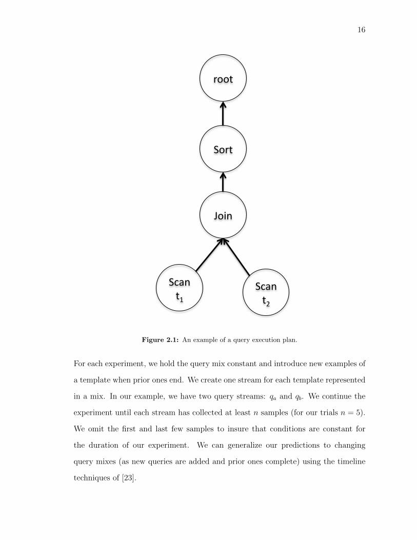
Much of our modeling revolves around taking apart the individual steps in a
query execution plan. This consists of a directed acyclic graph which allows the
query to compute its results. An example of a query execution plan is in Figure 2.1.
In this figure we see that we scan two tables, join and then sort them to return results
to the user. Tuples travel from the leaf nodes to the root using this technique. They
do so in a pipelined fashion, except when they meet blocking operators (such as the
sort).
For all of our concurrent trials we evaluate discrete mixes using a technique that
we call steady state. An example of a steady state sample is depicted in Figure 2.2.
16
!"#$%&'%
!"#$%&(%
)*+$%
!*,&%
,**&%
Figure 2.1: An example of a query execution plan.
For each experiment, we hold the query mix constant and introduce new examples of
a template when prior ones end. We create one stream for each template represented
in a mix. In our example, we have two query streams: qa and qb. We continue the
experiment until each stream has collected at least n samples (for our trials n = 5).
We omit the first and last few samples to insure that conditions are constant for
the duration of our experiment. We can generalize our predictions to changing
query mixes (as new queries are added and prior ones complete) using the timeline
techniques of [23].

17
!"# !"# !"#
!$# !$# !$# !$# !$#
%&'(#
Figure 2.2: An example of steady state query mixes, qa running with qb
Steady state evaluation allows us to reason about how a query will react to a
continuous level of contention and a fixed mix of queries. The warm cache (achieved
by omitting the first few samples) allows us to distill our measurements down to
interactions, rather than quantifying the overhead of the initial query set up and
caching of small supporting structures. This approach also causes us to sample the
changing interactions from queries overlapping at different phases in their execution.
2.2 Model-Based Predictions
To describe how query interactions occur we build regression models. These models
quantify the relationship between our indicators (such as logical I/O time) and the
value for which we are creating predictions (i.e., query latency). By determining
how these two quanities are correlated we can build robust predictions with limited
training sets.
For our models we begin with independent variables, or the ones that we use to
describe the phenonemon that we are modeling. We seek to find a simple relationship
between it and the dependent variable which we are forecasting. A considerable part
of our work is in understanding query interactions well enough to identify effective
independent variables for our analysis.
To build a model, we first begin with many (x, y) points, which we train upon.

18
Here x is a series of observations of indepenent variables and y are the corresponding
outcomes. We learn model coefficients to describe the relationship between x and y.
We use linear regression for the majority of our findings. Here we formulate what
we understand about our queries into a representation of how it impacts latency. The
majority of our models take the form y = mx + b and we solve for m, the slope of
our model and b the y-intercept of our model based on the training data.
In a select few cases we experiment with sophisticated machine learning tech-
niques. We do this to see if we can learn more complicated models of query interac-
tions by using all of the components of the QEP. In the rest of our work we primarily
focus on the leaf nodes because disk I/O is the main source of our interactions.
2.3 Model Quality Evaluation
We assessed the quality of our predictions using mean relative error (MRE):
MRE =1
n
n∑i=1
|observedi − predictedi|observedi
(2.1)
It is a normalized evaluation of accuracy. We quantify the scale of our errors in
terms of the quantity that we are trying to predict. This is an intuitive approach to
determining the accuracy of our frameworks.
An alternative that we considered was r2, the coefficient of determination (r2)
to assess the goodness of fit of the model to the data. R2 is a normalized measure
that relates the error of the model to the overall variance of the data set. It ranges
from 0 to 1, with higher values denoting a better model fit. It captures the error of
19
the model by calculating the sum-squared errors of each data point in the training
set (SSerr), normalized by the total variability of the data calculated by taking the
sum of squared deviates of the data points from the mean (SStot). r2 is calculated
as 1− SSerr/SStot.
Unless otherwise specified, we use k-folds cross validation to verify our work.
This technique divides the data into k equally sized folds. We train on k − 1 folds
and evaluate our model on the remaining one. We get a more complete picture of
our space using this technique while keeping our test and training data disjoint.
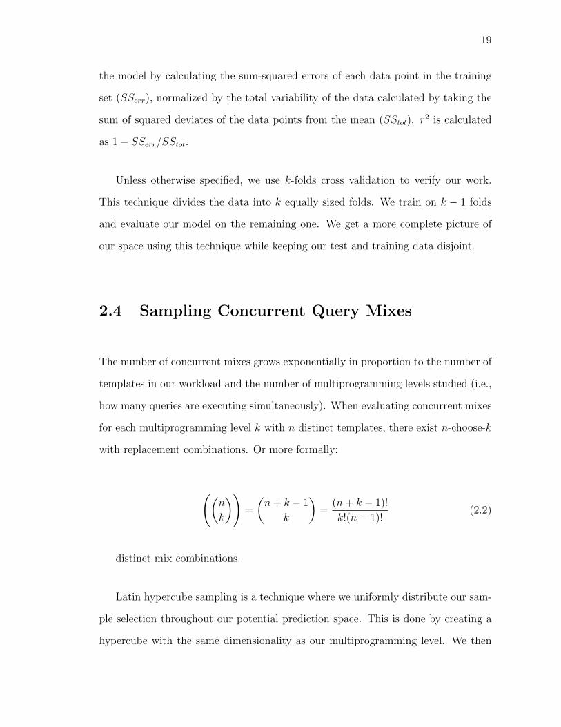
2.4 Sampling Concurrent Query Mixes
The number of concurrent mixes grows exponentially in proportion to the number of
templates in our workload and the number of multiprogramming levels studied (i.e.,
how many queries are executing simultaneously). When evaluating concurrent mixes
for each multiprogramming level k with n distinct templates, there exist n-choose-k
with replacement combinations. Or more formally:
((n
k
))=
(n+ k − 1
k
)=
(n+ k − 1)!
k!(n− 1)!(2.2)
distinct mix combinations.
Latin hypercube sampling is a technique where we uniformly distribute our sam-
ple selection throughout our potential prediction space. This is done by creating a
hypercube with the same dimensionality as our multiprogramming level. We then

20
Query 1 2 3 4 51 X2 X3 X4 X5 X
Table 2.1: Example of 2-D Latin hypercube sampling
select our samples such that every value on every plane gets intersected exactly once.
Each sampling run of this technique produces at most n combinations, where n is
the number of unique queries in our workload.
An example of Latin hypercube sampling is shown in Table 2.1. This example
demonstrates that each template gets sampled an equal number of times, in this
case twice. We can further sample the space by evaluating multiple, disjoint latin
hypercube samples.

Chapter Three
Concurrent Query Performance
Predictions for Static Workloads

22
In this section we examine the work that we did to predict cQPP for static worloads.
We presume for this section that all of the templates in our workload are well-defined
and build a distinct model for each based on its logical I/O latency patterns.
3.1 Modeling Discrete Query Mixes
Query latency is directly affected by resources contention in the underlying hardware
of the system on which it is executing. As the number of queries that are presently
executing goes up, they must increasingly share access to disk and CPU time as well
as RAM.
In this research we target OLAP workloads, thus we choose to focus on the
interaction of I/O and RAM for our latency predictions. We build an additive
multivariable model that estimates query interactions based on pairwise and isolated
observations. We use this model to estimate the average buffer access latency, which
we in turn use to estimate our end-to-end QoS.
3.1.1 Query Latency Indicators
We first study good indicators of query QoS. When we began researching contention,
we analyzed several examples of database-generated profiling data and experimented
with linear and power regression over several potential indicators of query latency.
The two indicators that we hypothesized showed most promise were I/Os consumed
and buffer pool misses.
We started by reasoning about what resources would experience the most con-

23
tention. We know that OLAP queries are highly I/O-bound. The process of fetching
pages for a database system is very complicated. From a simplified model we can
think of it as a hierarchy of access methods. When fetching a tuple for a query,
the executor first submits a request to the buffer pool, the smallest but fastest way
to access data. If the requested block is not found, the lookup is passed on to the
OS-level cache, which is the second fastest and smallest option. Finally, if this fails,
the request is enqueued for disk access to retrieve the block containing the requested
tuple. This disk access may be a seek or a sequential read, also causing the cost to
access a block of data to vary. This variance happens even when we know where
the block was found physically on disk. Our disk access time could potentially be
calculated as proportional to the position of a disk arm to simulate its motion to the
desired disk.
Needless to say, a system this complex is very challenging to model, but it does
break down into discrete steps. To capture this as an I/O vs RAM decision, we
started by looking at the number of blocks read from disk and how many buffer pool
misses were recorded.
The first metric we considered was quantifying the number of blocks read by a
query. We thought that if a query’s execution speed is highly tied to how fast it can
complete I/Os (and reads from RAM are essentially free), then this could give us an
indicator of how much query progress has been accomplished over time. We found
that there was a correlation between number of blocks read in a query’s execution
time and the query’s latency. Unfortunately it was a weak and noisy relationship,
due to the complexity of modeling the contents of RAM and variations in how far
the disk head had to move in order to access an arbitrary block.
Next we looked at buffer pool misses. We reasoned that the cost of disk access
24
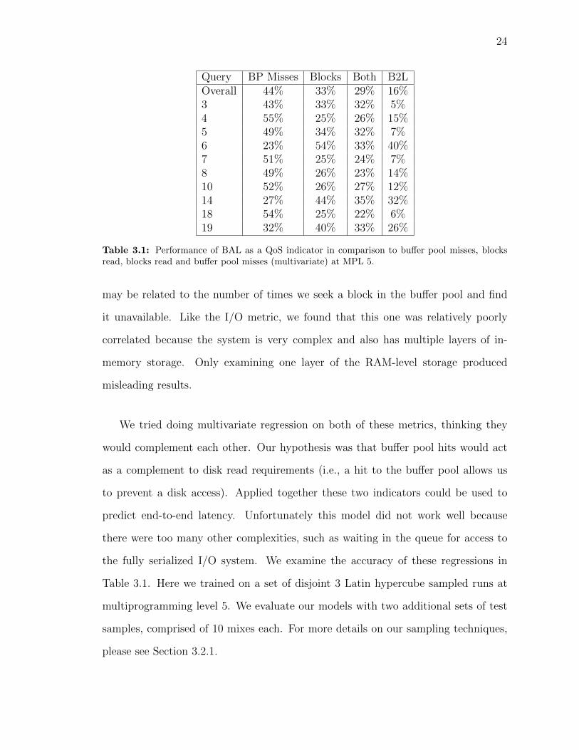
Query BP Misses Blocks Both B2LOverall 44% 33% 29% 16%3 43% 33% 32% 5%4 55% 25% 26% 15%5 49% 34% 32% 7%6 23% 54% 33% 40%7 51% 25% 24% 7%8 49% 26% 23% 14%10 52% 26% 27% 12%14 27% 44% 35% 32%18 54% 25% 22% 6%19 32% 40% 33% 26%
Table 3.1: Performance of BAL as a QoS indicator in comparison to buffer pool misses, blocksread, blocks read and buffer pool misses (multivariate) at MPL 5.
may be related to the number of times we seek a block in the buffer pool and find
it unavailable. Like the I/O metric, we found that this one was relatively poorly
correlated because the system is very complex and also has multiple layers of in-
memory storage. Only examining one layer of the RAM-level storage produced
misleading results.
We tried doing multivariate regression on both of these metrics, thinking they
would complement each other. Our hypothesis was that buffer pool hits would act
as a complement to disk read requirements (i.e., a hit to the buffer pool allows us
to prevent a disk access). Applied together these two indicators could be used to
predict end-to-end latency. Unfortunately this model did not work well because
there were too many other complexities, such as waiting in the queue for access to
the fully serialized I/O system. We examine the accuracy of these regressions in
Table 3.1. Here we trained on a set of disjoint 3 Latin hypercube sampled runs at
multiprogramming level 5. We evaluate our models with two additional sets of test
samples, comprised of 10 mixes each. For more details on our sampling techniques,
please see Section 3.2.1.

25
Buffer Pool Delay as a Performance Indicator (B2L)
We found that handling each of the I/O access cases individually had limited success
because the interactions were too complex. In an effort to distill the problem further,
we identified the initial request to the buffer pool as a gateway that all queries must
go through in order to receive data. When a query requests a block of data, it first
is added to a global queue maintained by the DBMS. When a request gets to the
top of the queue, then the system queries its levels of storage one after another until
it acquires the needed disk block.
!"
#!"
$!"
%!"
&!"
'!!"
'#!"
'$!"
'"
%%"
'('"
')%"
#%'"
(#%"
()'"
$*%"
*#'"
*&%"
%*'"
+'%"
+&'"
&$%"
)''"
)+%"
'!$'"
''!%"
''+'"
!"#$%&'(($))&*+,$-(.&/0)1&
!"#$%&2334&5$6"$),)&/789991&
Figure 3.1: BAL as it changes over time for TPC-H Query 14. Averaged over 5 examples of thetemplate in isolation.
Rather than modeling the steps of a buffer pool request, we reasoned that it would
be far simpler to estimate the time that elapses between when an I/O request is issued
and when the block of data is returned. We call this metric buffer access latency or
BAL. Averaging these latencies over the lifetime of a query gives us the ability to
summarize the interactions of disk seeks, sequential reads, OS cache hits and buffer
pool hits among disparate queries currently executing on the same database.
In Table 3.1 we examine the quality of BAL in comparison to the other indicators
we pursued to predict latency. We built linear regression models at multiprogram-
ming level 5 for blocks read, buffer pool misses, a multivariate regression model for
both and another model for BAL. Our experimental setup is detailed in Section 6.1.1.

26
Query Std Dev (µs)3 24.234 18.575 10.46 7.687 31.888 9.8710 23.4814 12.518 19.2919 10.1
Table 3.2: Standard deviation of BAL for various TPC-H queries.
We trained them all on a small set of disjoint data and this is the accuracy recorded
for test data, which has no overlap with the training data. BAL does roughly twice as
well as these other indicators, even when they are combined to build a model. BAL’s
accuracy improves further when we train it on samples from more multiprogramming
levels.
Our BAL indicator correlates strongly with latency because it is an average of our
logical page delay over a long period of time. An I/O bound query will have latency
directly proportional to how long it waits for I/O on average plus some fixed overhead
factor for CPU time and other inexpensive in-memory support operations. We use
linear regression to model this relationship between BAL and latency. It produces
an equation of the form y = mx+ b. Our system finds the overhead relatively fixed
on a per-query basis and it comprises the y-intercept (b) of the model. The m term
allows us to apply a cost to each I/O request we service in the course of our query
execution.
One of the reasons that BAL is a good indicator for latency is because it is
averaged over many samples over the lifetime of a query. Thus, even when a query
goes through very complex interactions with the OS as well as other queries, it will

27
still accurately predict the overall latency. In Figure 3.1 we display how the typical
values of BAL vary through the lifetime of a query when run in isolation. All of our
BAL measurements are averages of 1000 buffer pool requests. This particular query
(TPC-H Q14) goes through a brief period of low latency in BAL while the query
is warming up (it is scanning the probe relation for a hash join). Then it reaches
a relatively stable state where it is continuously reading in and joining tuples. The
BAL periodically fluctuates as the kernel context switches and experiences some
noise as it iterates through the join.
In Table 3.2, we look at the standard deviation for all of the queries from our
workload of ten moderate weight TPC-H queries. There are always outliers in the
BAL measurements due to the complexity of the system. Fortunately they are a
distinct minority of the measurement set for each query and thus their impact is
diminished by averaging. As the query 14 example demonstrates, we have a range
of 10-130 µs, but our standard deviation is only 12.5.
In summary, average BAL was our strongest indicator, so we chose to focus our
regression on its prediction. The strength of this model is demonstrated in its r2
values for each query class in our training. They varied from 0.877-0.994 for the
ten queries in our TPC-H workload. All of our queries were very well-fitted by
this modeling. We train on 175 template examples on average, using data from our
training sets at multiprogramming levels 1-5. Next we consider how to estimate this
execution speed, or BAL.

28
Variables R2
I 0.167I & C 0.169I & C & D 0.219I & C & D & G 0.358
Table 3.3: r2 values for different BAL prediction models (variables: Isolated (I), ComplementSum (C), Direct (D), Indirect (G))
. Training on multiprogramming level 3.
3.1.2 Resource contention prediction
At a higher level, we seek to quantify how a query’s performance changes as it ex-
periences resource sharing. In order to accomplish this we must first characterize
how a query class runs under optimal conditions, i.e., in isolation. We then need to
extrapolate how interacting with other query classes in our workload impacts its per-
formance. Quantifying contention is a very complex, multi-layered problem. Some of
the resources required are non-blocking (such as access to RAM or computing with
multiple cores), while others are serialized (including access to disk). Modeling all of
these facets of query execution and their interactions among each other analytically
is prohibitively expensive. We’d need to account for buffer pool state, CPU sharing,
and the more global state of the query executor. As we explored in the previous
section, average BAL is a consistent indicator of QoS, throughout changing query
mixes and concurrency levels. In this section we propose atechnique for predicting
average BAL byleveraging the interactions of query templates based onobservations
among pairs.
B2cB: Quantifying query interactions: a pairwise approach
To leverage B2Lfor end-to-end latency predictions, we must accurately predict the
average BAL. We start by examining the resource utilization of a query class un-

29
der optimal conditions (in isolation), what resources other queries that are running
concurrently will expect to consume and also quantify how much these queries will
contend with each other on a query-by-query basis (i.e., evaluating interactions as
pairs).
To better characterize how queries interact we first looked at all pairwise inter-
actions. For our workload of ten queries, we executed all 55 unique combinations
in steady state. These pairings allowed us to characterize the magnitude and sign
(positive or negative to denote slow down or speed up respectively) for each pairwise
interaction in the workload. For example, when TPC-H Query 19 is run with Query
7 it executes in roughly the same amount of time it does in isolation. This is because
both of their query execution plans are dominated by sequential scans on the fact
table. In contrast, when Q19 is run with Q7, it slows down by approximately 50%.
In this case, the two queries share less overlap in their working sets and both require
significant RAM to do expensive joins.
We use this base pairwise interaction rate and isolated runs to build our regression
model. Specifically, we predict the average BAL based on these two inputs. We have
found that as long as we do not reach a state of overload, concurrency has an additive
effect on delay. We call this BAL estimation system ”BALs to concurrent BAL” or
B2cB.
When we predict the latency or BAL of a query, we call this query the primary.
Queries that are running concurrently with it are its complements.
Our model has the following four independent variables, provided from training
data of queries running in steady state as pairs as well as in isolation:

30
• Isolated : Isolated BAL of primary query
• Complements : Sum of complement queries’ isolated BALs
• Direct : Sum of the change in BAL for the primary when it interacts with each
of its complements
• Indirect : Sum of indirect contention costs, i.e., the change in BAL for each
complement with each other complement.
The intuition behind this model is that when we are dealing with a non-overloaded
state, the cost of contention increases linearly, and is a function of fixed costs for
each query in the mix as well as variable costs for each pairwise interaction among
the queries (a roughly n2 relationship, divided into direct and indirect costs). If
we presume round robin scheduling, then the BAL becomes the cost of our initial,
isolated reading, plus the cost of one average reading of each of the complements,
plus observed interaction costs among all of the queries in the workload.
Examining isolated BAL creates a baseline to assess the concurrent BAL. It pro-
vides us the default access time for the primary query, under optimal circumstances.
We are summarizing the behavior of an very complex system by estimating how long
on average it takes to access a block of data for the query executor. We denote the
isolated BAL of a query i as Ti.
Similarly, we need to consider the needs of the complement queries that are
running in our proposed mix. Summing the BAL of the complements allows us
to build an estimate of the rate at which they consume I/O bandwidth given fair
scheduling. This is a rough estimate of the “cost” of complement queries. A fast
isolated average BAL implies that we have a lightweight query that draws most of
its inputs from RAM. In contrast, longer buffer access latencies mean that a query

31
is requesting diverse data that is not memory- resident such as a fact table scan or
an index scan, necessitating expensive seeks.
Next we look at the change in BAL for our direct query interactions. We quantify
a direct query interaction as the average BAL of a query when it is measured in steady
state with one other query. We refer to the BAL of query i run with query j as Ti/j.
We take the change in this measurement as ∆Ti/j = Ti/j − Ti. If this quantity is
positive, we are experiencing slowdown. If it is negative then we have a beneficial
interaction between queries. As alluded to earlier, like queries (especially ones in the
same query class) sometimes help each other finish faster. In contrast, queries that
access completely different relations will only create contention and can dramatically
slow down query execution progress.
Finally we examine the change in delay between the complement queries. This
gives us a glimpse into how much contention they are creating and how much their
interacting footprint will affect the primary query. It is worth noting that their
interactions may not be symmetrical (∆Ti/j 6= ∆Tj/i. For example, an equi-join
requires dedicated memory to complete their comparisons efficiently. If it is run
concurrently with a table scan, the table scan will not be as affected by the join
because it uses each tuple only once. The scanning query disproportionately affects
the latency of the joining query due to it having access to less memory.
We found that all of these independent variables were necessary to build a com-
plete model. As Table 3.3 demonstrates, our R2 increases significantly once we start
considering isolated costs with interactions, and has almost half the sum-squared
error when solving for four variables rather than relying on the isolated BAL as an
indicator.

32
We predict average BAL for query q, with the remaining queries in the mix (com-
plements) as c0..cn as:
B = αTq + β
n∑i=0
Tci + γ1
n∑i=0
∆Tq/ci + γ2
n∑i=0
n,j!=i∑j=0
∆Tci/cj (3.1)
We solve for the coefficients α, β, γ1 and γ2 using linear multivariate regression
for all queries in our training set, once per each multiprogramming level. We elect to
do this regression once per multiprogramming level to make a robust model for many
query interactions. The regression technique derives our coefficients using the least
sum-squared error method. Our samples are derived from latin hypercube sampling.
An example of this technique is Table 2.1.
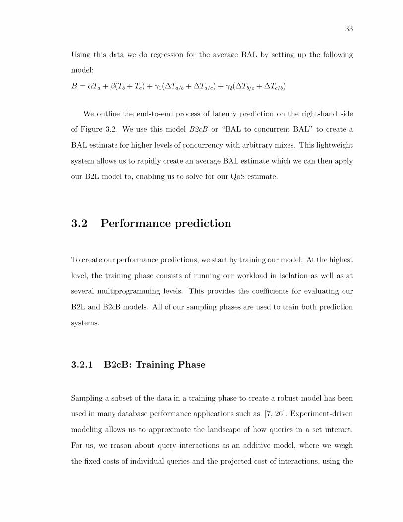
Figure 3.2: System model for query latency predictions in steady state.
To provide a more concrete example, if we are predicting the BAL of query a
and it is being run with queries b and c, we start out with the following inputs:
• Ta, Tb, Tc - the average BAL of a, b and c when run in isolation
• ∆Ta/b,∆Ta/c, et cetera - change in BAL of a when run with b or c (∆Ta/b =
Ta/b − Ta)
33
Using this data we do regression for the average BAL by setting up the following
model:
B = αTa + β(Tb + Tc) + γ1(∆Ta/b + ∆Ta/c) + γ2(∆Tb/c + ∆Tc/b)
We outline the end-to-end process of latency prediction on the right-hand side
of Figure 3.2. We use this model B2cB or “BAL to concurrent BAL” to create a
BAL estimate for higher levels of concurrency with arbitrary mixes. This lightweight
system allows us to rapidly create an average BAL estimate which we can then apply
our B2L model to, enabling us to solve for our QoS estimate.
3.2 Performance prediction
To create our performance predictions, we start by training our model. At the highest
level, the training phase consists of running our workload in isolation as well as at
several multiprogramming levels. This provides the coefficients for evaluating our
B2L and B2cB models. All of our sampling phases are used to train both prediction
systems.
3.2.1 B2cB: Training Phase
Sampling a subset of the data in a training phase to create a robust model has been
used in many database performance applications such as [7, 26]. Experiment-driven
modeling allows us to approximate the landscape of how queries in a set interact.
For us, we reason about query interactions as an additive model, where we weigh
the fixed costs of individual queries and the projected cost of interactions, using the

34
B2cB method from Section 3.1.
Our model must evaluate contention at three levels: isolation, pairwise and higher
degrees of concurrency. The steps are displayed in Figure 3.2.
First we characterize the workload that we have in terms of how each query
behaves in isolation. This baseline allows us to get an estimate of what constitutes
normal, unimpeded progress for a query class and how much we are speeding up or
slowing down as more queries are added too the mix. We collect 5 samples of each
query class running in isolation with a warm cache. We record both the latency
and BAL for our model building. The BAL provides input for the first two terms of
the B2cB model. The BAL-latency pair is used in the training of the B2L latency
prediction model.
Next, we build a matrix of interactions by running all pairwise combinations, 55
in our case. This allows us to succinctly estimate the degree of contention that each
query class in a workload puts on every potential complement. As with our isolated
measurements, we get both end-to-end latency as well as average BAL measurements
for all of these combinations. These BAL-latency pairs are also used for the B2L
training phase. In addition, they too are used as inputs for the examples used by
B2cB to estimate BAL. This moderate number of samples is completely necessary
for both our BAL and latency predictions. The pairwise interactions provide us with
inputs for the independent variables of B2cB. They also give us our input for our
B2L model. B2L builds upon many concurrency levels in order to plot how latency
grows as contention increases. Each multiprogramming level helps us complete the
model.
After that we build our model coefficients for interactions of degree greater than 2.

35
This linear regression is done on a set of Latin hypercube sampled data points. These
sample runs are used to create the coefficients for B2cB at each multiprogramming
level.
LHS is a general sampling technique and is not a perfect fit for exploring this
space of all possible query combinations. LHS does not take into account the differ-
ence between combinations and permutations when exploring our sampling space.
For example, to the sampler, the combination of (3, 4) and (4, 3) would both be
considered distinct samples. From the database’s point of view they are both simply
one instance of Q3 and one instance of Q4 running concurrently. We eliminated LHS
in which the same combination appears more than once from our training set.
For our training phase we used this sampling technique three times for each
concurrency level. Experimentally we found that as more samples were taken we
naturally get a more comprehensive picture of the cost of contention in our system.
On the other hand, more sampling takes more time. We found that three LHS
runs for each multiprogramming level was a good trade off between these competing
objectives. Acquiring more samples did not improve our prediction accuracy by
greater than 5%.
Each LHS run consists of ten steady state combinations, resulting in 30 training
combinations sampled for each multiprogramming level. Initially this may seem like
a lot of samples, but realize that it is not that many in comparison to all possible
combinations. This is especially true for higher multiprogramming levels where our
set of combinations grows exponentially every time we add a query.
In practice, the total training period took approximately a couple of days in our
modest setup. This may seem like considerable time, but we are only required to
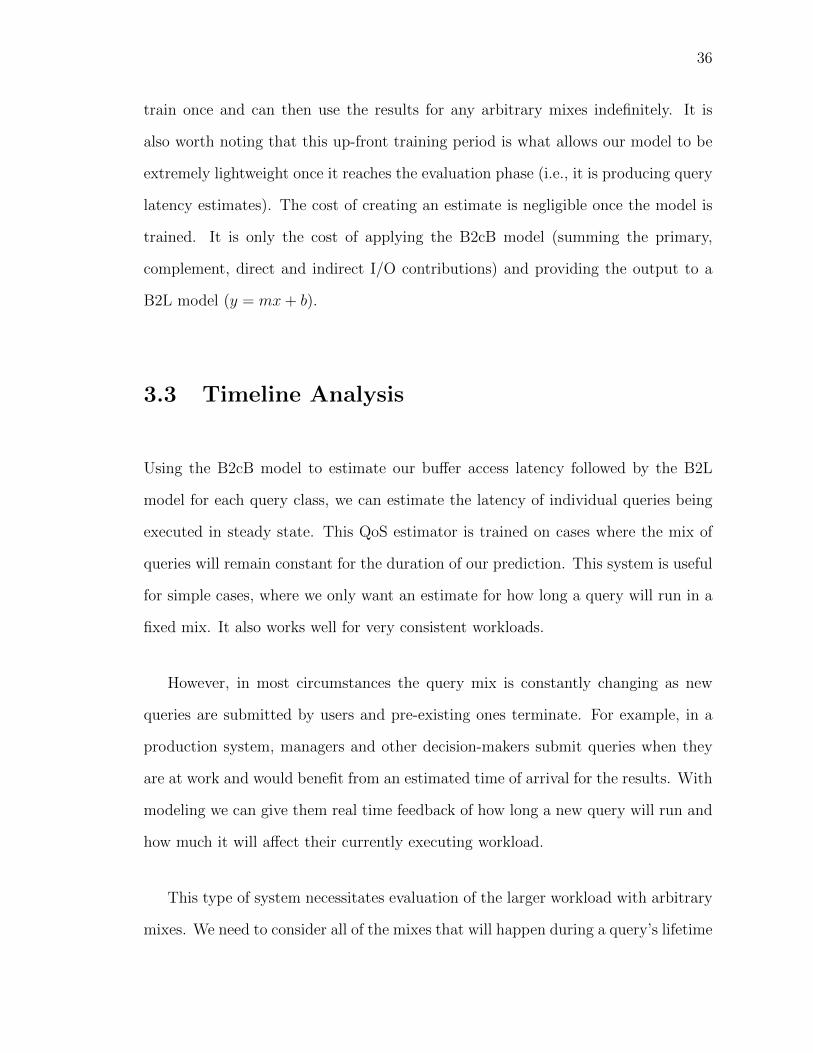
36
train once and can then use the results for any arbitrary mixes indefinitely. It is
also worth noting that this up-front training period is what allows our model to be
extremely lightweight once it reaches the evaluation phase (i.e., it is producing query
latency estimates). The cost of creating an estimate is negligible once the model is
trained. It is only the cost of applying the B2cB model (summing the primary,
complement, direct and indirect I/O contributions) and providing the output to a
B2L model (y = mx+ b).
3.3 Timeline Analysis
Using the B2cB model to estimate our buffer access latency followed by the B2L
model for each query class, we can estimate the latency of individual queries being
executed in steady state. This QoS estimator is trained on cases where the mix of
queries will remain constant for the duration of our prediction. This system is useful
for simple cases, where we only want an estimate for how long a query will run in a
fixed mix. It also works well for very consistent workloads.
However, in most circumstances the query mix is constantly changing as new
queries are submitted by users and pre-existing ones terminate. For example, in a
production system, managers and other decision-makers submit queries when they
are at work and would benefit from an estimated time of arrival for the results. With
modeling we can give them real time feedback of how long a new query will run and
how much it will affect their currently executing workload.
This type of system necessitates evaluation of the larger workload with arbitrary
mixes. We need to consider all of the mixes that will happen during a query’s lifetime
37
as the number and/or type of complement queries goes up and down. This system
must quantify the slowdown (or speedup) caused by these mixes, and estimate what
percentage of the query’s work will happen in each mix.
We propose two scenariosfor evaluating our predictions. The first setup we study
is one in which new queries are being submitted for immediate execution. In this case
we presume that at scheduling time the number of queries executing monotonically
decreases as the queries currently executing complete. In the second scenario we
consider a batch-based approach, where our system is given a fixed multiprogram-
ming level and a queue of queries to run. In this method we also attempt to model
the mixes that will occur, by projecting when queries from the queue will started
during the time we are modeling in our prediction.
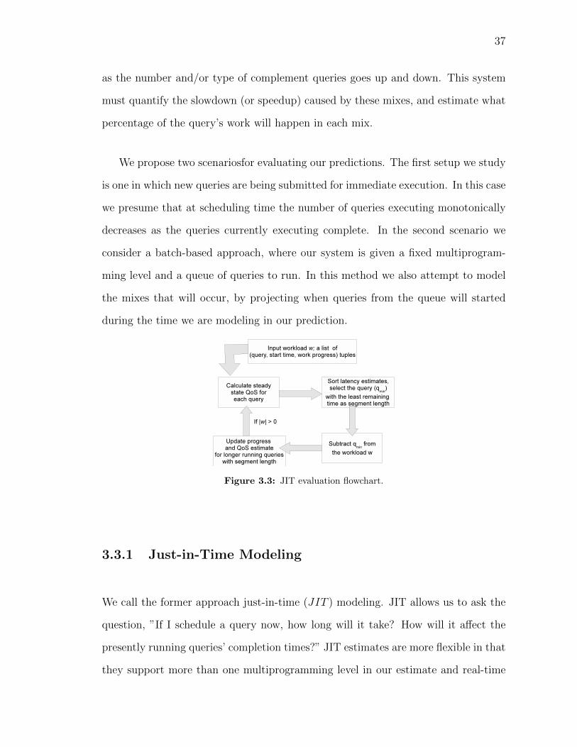
Figure 3.3: JIT evaluation flowchart.
3.3.1 Just-in-Time Modeling
We call the former approach just-in-time (JIT ) modeling. JIT allows us to ask the
question, ”If I schedule a query now, how long will it take? How will it affect the
presently running queries’ completion times?” JIT estimates are more flexible in that
they support more than one multiprogramming level in our estimate and real-time

38
changes in the workload.
Also, this more incremental approach will allow us to refine our estimates as
time goes on. As we evaluate QoS every time a query is added, we can correct
past estimates by examining how the query has progressed since we last forecasted
its end-to-end latency. In the context of a SLA, this may allow us to prevent QoS
violations from happening by giving us time to intervene and load balance as we go
along. Experimentally we saw an average of 9% accuracy in our QoS estimates with
this approach.
This timeline generation requires estimates of the latency for each query in each
mix and what percentage of its execution time each mix will occupy. When we
evaluate individual steady states, we infer an ordering of when queries will terminate
by sorting their remaining latency estimates. It is updated whenever a query is added
to our workload to estimate how long a new query will run and how it will impact
its complements.
The JIT algorithm is charted in Figure 3.3. In our timeline-based QoS estimator,
first we look at all of the progress of the n queries that are presently executing in
a mix. We create a list of the time that has elapsed since each presently executing
query began and initialize our performance estimate with this quantity. We also
record the number of buffer pool requests that have been serviced in the past for
each query. This second metric gives us a rough estimate of what percentage of the
query’s work has been completed.
Next we must look at the estimated QoS for each query in the proposed mix,
operating under the temporary assumption that the mix does not change. We can
use the techniques in the previous section to create end-to-end latency estimates for

39
each query in the workload under these steady state conditions. This first estimates
BAL using B2cB, which we then translate into latency using B2L.
After this we sort the steady state estimates and pick the query with the minimum
remaining time as our first segment of evaluation. This defines the period over which
we evaluate our first discretemix. We select this qmin and its estimated latency lmin
as the time when our mix state will change next. We then subtract qmin from the
mix.
We then update the progress of each query that is not equal to qmin by taking the
ratio of lmin/lq and multiplying it by the buffer pool requests remaining for query
q. We also add lmin to our estimate for each query in the workload that is not
terminating.
As an aside, we found that our buffer pool request count never varied more than
5% for the same query class. This is because the query execution plan never changed,
despite the use of range queries and indices. If a query did exhibit plan changes,
either caused by a skewed distribution of the data or more variable range queries,
we can account for this by subdividing our query classes into cases for each plan /
range.
Finally, we subtract qmin from our workload because we project that it will have
ended at this prediction point. We keep iteratively predicting and eliminating the
query with the least time remaining until we have completed our estimates for all
queries in the workload.
To summarize, we start with n queries and project a completion time for each in
n phases. Each phase contains a monotonically decreasing multiprogramming level
40
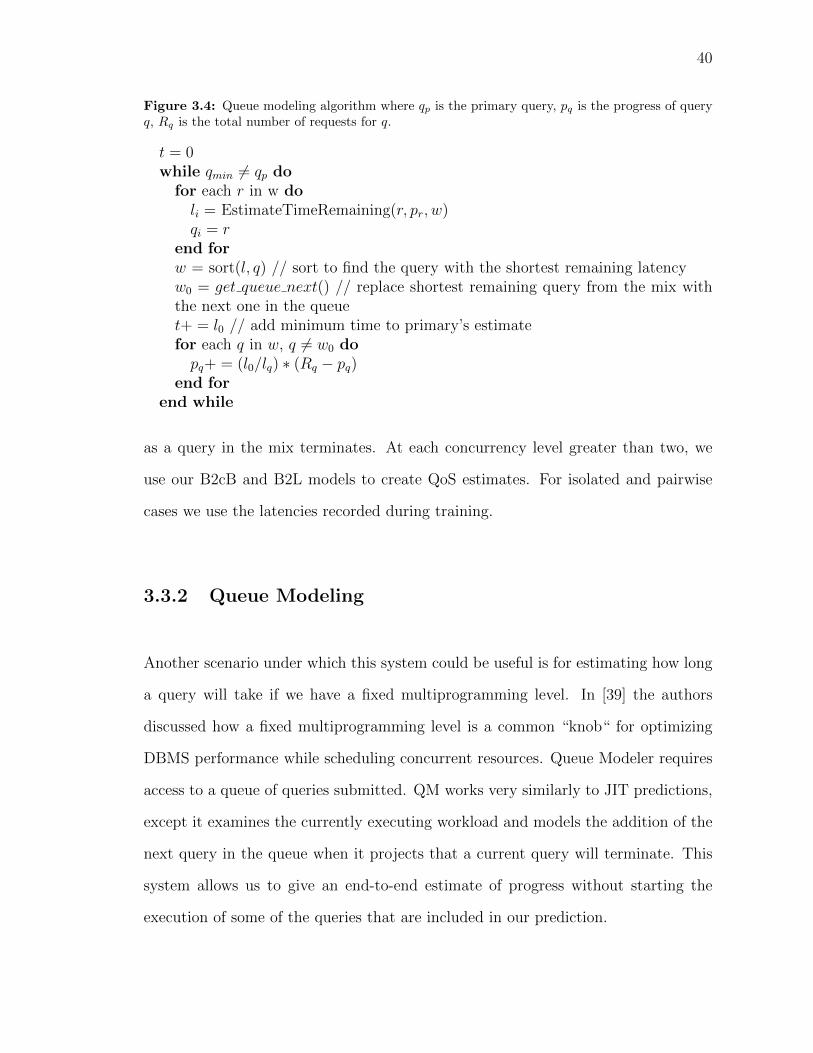
Figure 3.4: Queue modeling algorithm where qp is the primary query, pq is the progress of queryq, Rq is the total number of requests for q.
t = 0while qmin 6= qp do
for each r in w doli = EstimateTimeRemaining(r, pr, w)qi = r
end forw = sort(l, q) // sort to find the query with the shortest remaining latencyw0 = get queue next() // replace shortest remaining query from the mix withthe next one in the queuet+ = l0 // add minimum time to primary’s estimatefor each q in w, q 6= w0 dopq+ = (l0/lq) ∗ (Rq − pq)
end forend while
as a query in the mix terminates. At each concurrency level greater than two, we
use our B2cB and B2L models to create QoS estimates. For isolated and pairwise
cases we use the latencies recorded during training.
3.3.2 Queue Modeling
Another scenario under which this system could be useful is for estimating how long
a query will take if we have a fixed multiprogramming level. In [39] the authors
discussed how a fixed multiprogramming level is a common “knob“ for optimizing
DBMS performance while scheduling concurrent resources. Queue Modeler requires
access to a queue of queries submitted. QM works very similarly to JIT predictions,
except it examines the currently executing workload and models the addition of the
next query in the queue when it projects that a current query will terminate. This
system allows us to give an end-to-end estimate of progress without starting the
execution of some of the queries that are included in our prediction.
41
We detail the working of Queue Modeler in Algorithm 3.4. Queue modeling starts
with a list of status information for each presently executing query, much like JIT.
This too is a pair of the query execution time and the progress the query has made
in terms of buffer pool requests. We add the new query to the list with its progress
and current latency at zero. Next we model the steady state latency of each query
in the mix and sort the remaining latency estimates. We then replace the query
that has the shortest remaining time (qmin) with the next one on the queue. qmin
is projected to continue running for rmin time. Next we update the progress of the
remaining queries by taking the ratio of rmin to their projected time remaining. We
continue this cycle until the query for which where are creating a prediction is qmin.

Chapter Four
Generalized Concurrent Query
Performance Prediction
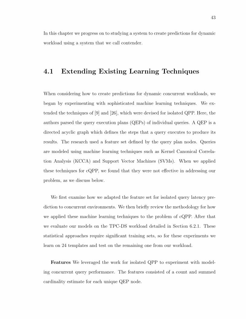
43
In this chapter we progress on to studying a system to create predictions for dynamic
workload using a system that we call contender.
4.1 Extending Existing Learning Techniques
When considering how to create predictions for dynamic concurrent workloads, we
began by experimenting with sophisticated machine learning techniques. We ex-
tended the techniques of [9] and [26], which were devised for isolated QPP. Here, the
authors parsed the query execution plans (QEPs) of individual queries. A QEP is a
directed acyclic graph which defines the steps that a query executes to produce its
results. The research used a feature set defined by the query plan nodes. Queries
are modeled using machine learning techniques such as Kernel Canonical Correla-
tion Analysis (KCCA) and Support Vector Machines (SVMs). When we applied
these techniques for cQPP, we found that they were not effective in addressing our
problem, as we discuss below.
We first examine how we adapted the feature set for isolated query latency pre-
diction to concurrent environments. We then briefly review the methodology for how
we applied these machine learning techniques to the problem of cQPP. After that
we evaluate our models on the TPC-DS workload detailed in Section 6.2.1. These
statistical approaches require significant training sets, so for these experiments we
learn on 24 templates and test on the remaining one from our workload.
Features We leveraged the work for isolated QPP to experiment with model-
ing concurrent query performance. The features consisted of a count and summed
cardinality estimate for each unique QEP node.

44
We extended these feature sets for cQPP two ways. First, we made them
interaction-aware by incorporating data describing the specific I/O requirements
of individual QEPs. We performed this by adding a feature for each distinct table
scanned. Second, we made it concurrency-aware by adding the features of contem-
porary queries. This brings our total number of features up to 4n, where n is the
number of distinct QEP nodes including sequential scans for each table. In our
experiments, we had 168 features for 42 QEP node types. This resulted in very
complex models as we cast our queries into a high dimensional space.
Accuracy We evaluated two popular machine learning techniques to create pre-
dictions for new templates based on the features described above. In the first tech-
nique, KCCA, we create predictions by identifying similar examples in the training
data. In the second technique, SVM, we learn by classifying queries by their features
to coarse-grained latency labels. For both cases, we work at the granularity of the
query plan and we used well-known implementations of each technique [14, 33].
We found moderate success with this approach for static workloads at MPL 2
(i.e., with the same templates in the training and test set but differing concurrent
mixes). We trained on 250 concurrent query mixes and tested on 75 mixes, giving us
a 3.3 : 1 ratio of training to test data. Each template was proportionally distributed
between the training and test set. We found that we could predict latency within
32% of the correct value with KCCA on average and within 21% for SVM. While
these results are competitive with the work of [23], they are more complex and time
consuming in comparison to their predecessors.
We also evaluated these approaches on a dynamic workload. For this study, we
reduced our workload from 25 to 17 templates because the remaining 7 templates
had one or more QEP nodes that were not present in any other template in our

45
!"#
$!"#
%!"#
&!"#
'!"#
(!"#
)!"#
*!"#
+!"#
,!"#
$!!"#
-./# %# $(# $*# %!# %%# %(# %)# %*# &%# ')# ()# )!# )$# )(# *$# *,# +%#
!"#$%&"
'#()"%*++,+%
-"./'#0"%
011-#
234#
Figure 4.1: Relative error for predictions at MPL 2 using machine learning.
workload. We could not build models for features that we have not trained upon.
As shown in Figure 4.1, we found that neither technique was very good at esti-
mating latency for previously unseen templates. KCCA was very sensitive to changes
in QEP nodes used because it takes the Euclidean distance between the new tem-
plate and all of the training examples. When a new template is far in feature space
from all of our training examples, its predictions are of lower quality. Likewise, SVM
was over-fitting the templates that it has rather than learning interactions between
QEP nodes. This is problematic because nodes that are salient in one QEP may be
absent in others.
Both techniques perform well on queries where they have one or more templates
that are close in plan structure (e.g., templates 56 and 60). In this context, we
found that machine learning solutions work proportionally to the quality of their
training data. Unfortunately QEP feature space is sparsely populated in practice, so
building a robust model of this space is very time consuming. Thus, we propose an
alternative approach that casts the problem in terms of resource contention rather
than individual node interactions.

46
4.2 Modeling Resource Availability
In this section we describe how we model I/O availability to predict the latency of
a query t (the primary query) when executing concurrently with a query set C (the
contemporary queries). First, we discuss how we generate a latency range for the
primary based on the minimal and maximum I/O contention. We refer to this range
as the primary’s performance continuum. Then we study how we can estimate where
in this range the primary’s performance lies by modeling the I/O contention between
the primary query and its contemporaries.
In our models we elected to work at the level of the template rather than indi-
vidual query execution plans. The reasons for this are twofold. First, as discussed
in Section 4.1, modeling interactions at the QEP level is not fruitful using conven-
tional techniques. Secondly, we observed that on average our templates exhibited a
standard deviation in latency of 6% when executing in isolation, which is a manage-
able deviation. Were we to find higher variance, we could use the techniques in [5]
to divide our templates into subclasses. In this work we focus on the interactions
among query templates, rather than the individual query characteristics.
4.2.1 Template Performance Continuum
Contender creates a continuum that establishes a range for the performance of the
primary query template. To make performance comparable to other templates, we
normalize the query’s latency as a percentage of its continuum and we estimate
the upper and lower performance by simulating the best and worst I/O contention
scenario. By quantifying where a template’s performance lies on the continuum, we
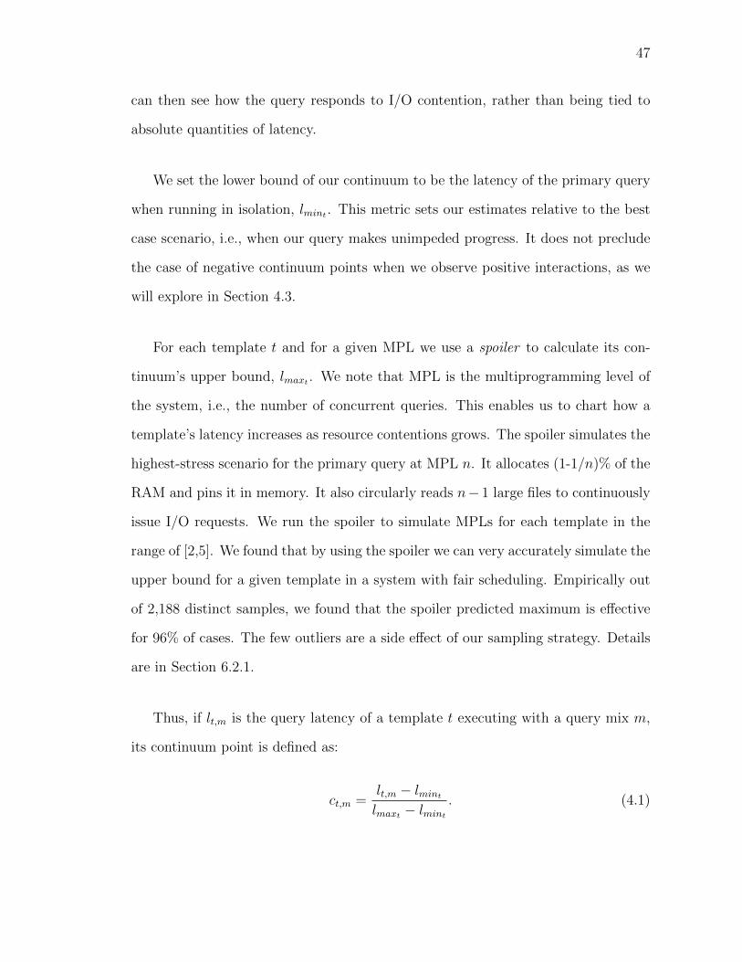
47
can then see how the query responds to I/O contention, rather than being tied to
absolute quantities of latency.
We set the lower bound of our continuum to be the latency of the primary query
when running in isolation, lmint . This metric sets our estimates relative to the best
case scenario, i.e., when our query makes unimpeded progress. It does not preclude
the case of negative continuum points when we observe positive interactions, as we
will explore in Section 4.3.
For each template t and for a given MPL we use a spoiler to calculate its con-
tinuum’s upper bound, lmaxt . We note that MPL is the multiprogramming level of
the system, i.e., the number of concurrent queries. This enables us to chart how a
template’s latency increases as resource contentions grows. The spoiler simulates the
highest-stress scenario for the primary query at MPL n. It allocates (1-1/n)% of the
RAM and pins it in memory. It also circularly reads n− 1 large files to continuously
issue I/O requests. We run the spoiler to simulate MPLs for each template in the
range of [2,5]. We found that by using the spoiler we can very accurately simulate the
upper bound for a given template in a system with fair scheduling. Empirically out
of 2,188 distinct samples, we found that the spoiler predicted maximum is effective
for 96% of cases. The few outliers are a side effect of our sampling strategy. Details
are in Section 6.2.1.
Thus, if lt,m is the query latency of a template t executing with a query mix m,
its continuum point is defined as:
ct,m =lt,m − lmint
lmaxt − lmint
. (4.1)

48
Symbol Definitionlmint minimum latency of template tlmaxt maximum latency for template tpt % of exec. time t uses I/O in isolationsf time required to scan table f in isolationla,m observed latency of template a when run in mix mhf times that f appears in a mix’s fact table scansgf,c boolean for if c and primary scans fjf,c boolean for if c scans f and the primary does notωc I/O time executed by contemporary c and primaryτc I/O time in which contemporary c executes shared
scans with other contemporariesrc query intensity for contemporary crt,m CQI for primary t in mix m
Table 4.1: Notation for CQI model for a query t, table scan f and contemporary query c.
Contender predicts the continuum point, ct,m, and then based on Equation 4.1
estimates the latency, lt,m, of the primary query t. In the next sections we present
our prediction model for ct,m, which is based on modeling the impact of resource
availability on the latency of the primary query t.
4.2.2 Contemporary Query Intensity (CQI)
Given a primary query t executing concurrently with a set of contemporary queries
C = {c1, ..., cn}, Contender uses the CQI metric to model how aggressively con-
current queries will use the underlying resources. Specifically, we focus on how to
accurately model the usage of I/O by the contemporary queries. This is important
because the I/O bottleneck is the main source of analytic query slowdown [23]. We
first examine how much of the I/O bandwidth each contemporary query uses when
it has no contention. We then estimate the impact of shared scans between the
primary t and its contemporaries C. Finally we evaluate how shared I/O among the
contemporaries may further ameliorate I/O scarcity.

49
Baseline First, we examine the behavior of each contemporary template ci by
quantifying its I/O requirements. Specifically, we measure the percent of the query’s
execution time spent executing I/O in isolation, pci . We do not differentiate between
sequential versus random I/O, deliberately measuring the query in terms of only the
time required on the I/O bus. Using this metric, we evaluate I/O in the same units
as latency. We calculate pci by measuring the time the disk has spent executing I/O
while the query ci is running in isolation. (we used Linux’s procfs statistics). Our
first approximation of the I/O requirements of our contemporaries can be calculated
by averaging pci for all of the contemporary queries c1, ..., cn.
Positive Primary Interactions After we have a baseline estimate for the I/O
requirements of our contemporary queries, we focus on estimating the positive impact
of interactions on the each contemporary query ci. One way for a query ci to have
less contention is for it to share work with its primary query. Sharing needs to be
large enough for the interaction to make an impact on end-to-end latency. The bulk
of our positive interactions will occur from shared fact table scans which are at the
heart of our interactions. These are the largest source of I/O usage for analytical
queries and the ones that are most subject to reuse in shared buffers.
Therefore, for each contemporary query we estimate its I/O behavior as it in-
teracts with the primary. Specifically, we estimate the time spent on I/Os that are
shared between the primary and its contemporary queries. We estimate this time
by first determining the fact tables scans that are shared by the primary and each
contemporary ci as:
gf,ci =
1 if template ci and primary both scan table f
0 otherwise

50
Then, we can estimate the time that the contemporary template ci will no longer
exclusively require for I/O, ωci (since these I/O requests are shared with the primary),
as:
ωci =n∑f=1
gf,ci × sf (4.2)
where sf is the table scan latency for the fact table f . We empirically evaluate
the latency of each table scan by executing a query consisting of only the sequential
scan. The above formula sums up the estimated time required for each shared fact
table scan.
Contemporary Interactions In addition to determining the I/O that is likely
to be shared between the primary and its contemporaries, we must also forecast
the work that will be shared among contemporaries. For example, if our primary is
executed with contemporaries a and b, we want to take into account the savings in
I/O time for any scans that are shared by a and b.
We first determine the table scans that are shared between ci and its non-primary
contemporaries with:
jf,ci =
1 if ci scans f , the primary does not and hf > 1
0 otherwise
where hf counts the number of contemporaries sharing a scan table f . Because we
are only interested in shared scans, we add the limit that hf must be greater than
one. We also require that fact table f must not appear in the primary to avoid double
counting. We estimate that on average the intersecting templates will equally split
the cost of the sequential scans. We can calculate the reduction in I/O due to shared

51
scans for each contemporary c as:
τci =n∑f=1
jf,ci × (1− 1
hf)× sf (4.3)
Contemporary I/O Requirements Given the I/O requirements reductions
due to positive interactions with the primary and the non-primary contemporaries,
we can estimate the I/O requirements of a contemporary query ci as:
rci = (lminci× pci − ωci − τci)/lminci
(4.4)
Here, we take the latency of ci executing in isolation (lminci). We multiply it by
pci , the percentage the query spend executing I/Os, to estimate its I/O time. We then
subtract its positive interactions with the primary and other contemporaries. This
gives us an estimate of the percentage of ci’s “fair share” of hardware resources that it
will use and it reduces the I/O requirements to that which is strictly interfering with
the primary. Contemporaries with high rci values will use most or all of the resources
available to them, bringing the primary closer to the spoiler provided maximum. A
lower rci indicates a query that will create little contention for the primary.
We then average the r values over all contemporaries to produce rt,m for primary
t in mix m, where m is comprises the primary and contemporaries c1, ..., cn:
rt,m =1
n
n∑i=1
rci (4.5)
rt,m is our Contemporary Query Intensity (CQI) metric, which we use to model the
I/O contention for the primary t. We truncate all negative I/O requirements to zero.
This occurs when contemporaries have negligible I/O requirements outside of their

52
!"#$
"%$
&"$
"#$
'"#$()$*+,-"#
."#$/$!"
#$0$&"
#12*+,-"#
$
3$
Figure 4.2: An example of calculating query intensity for an individual contemporary.
p p + ω p + ω + τMPL 2-5 25.4% 20.4% 20.2%
Table 4.2: Mean relative error for the CQI model for latency prediction.
shared scans. We use this estimate as the independent variable for our predictions
of the primary’s continuum point, ct,m (see Section 4.3).
To work through an example, see Figure 4.2. Here c1 shares one fact table scan
with the primary t and one with the contemporary c2. First contender calculates
the baseline I/O bandwidth for c1 as lminc1× pc1 . We then subtract the duration
of the one shared scan with the primary as ωc1 . After that we subtract half of its
shared scan with c2 as τc1 , to account for savings among the contemporaries. We
then divide by lminc1to estimate the percentage of I/O time that c1 will require.
Latency Prediction based on CQI In Table 4.2 we analyze how well CQI
predicts latency based on linear regression. We start with the baseline and incre-
mentally add the the primary and contemporary interactions to our CQI estimate.
We examine our ability to predict latency at MPLs 2-5. In the first column, we
examine having our independent variable be only the average percent of I/O time
used by the contemporary queries. Here, we theorized that if we knew how much
of the I/O bandwidth each contemporary query would use in isolation, we could av-
erage it out to determine the amount of “slack” available. This approach produced
moderately good predictions at 25%.
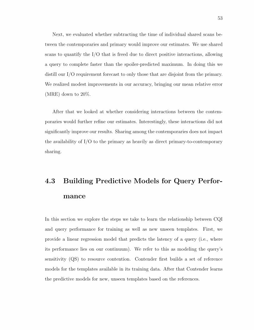
53
Next, we evaluated whether subtracting the time of individual shared scans be-
tween the contemporaries and primary would improve our estimates. We use shared
scans to quantify the I/O that is freed due to direct positive interactions, allowing
a query to complete faster than the spoiler-predicted maximum. In doing this we
distill our I/O requirement forecast to only those that are disjoint from the primary.
We realized modest improvements in our accuracy, bringing our mean relative error
(MRE) down to 20%.
After that we looked at whether considering interactions between the contem-
poraries would further refine our estimates. Interestingly, these interactions did not
significantly improve our results. Sharing among the contemporaries does not impact
the availability of I/O to the primary as heavily as direct primary-to-contemporary
sharing.
4.3 Building Predictive Models for Query Perfor-
mance
In this section we explore the steps we take to learn the relationship between CQI
and query performance for training as well as new unseen templates. First, we
provide a linear regression model that predicts the latency of a query (i.e., where
its performance lies on our continuum). We refer to this as modeling the query’s
sensitivity (QS) to resource contention. Contender first builds a set of reference
models for the templates available in its training data. After that Contender learns
the predictive models for new, unseen templates based on the references.

54
4.3.1 Modeling the Continuum: Estimating Query Sensitiv-
ity (QS)
Table 4.2 shows that we can build highly accurate predictions using linear regression
based on CQI. We can estimate CQI using Equation 4.5 which is built on a blend of
semantic query plan information and physical measurements in isolation, as described
in Section 4.2. Given the CQI, we can build a second model to predict the relationship
between CQI and a template’s performance (i.e., its continuum point) for a given
mix of concurrent queries.
We learn the relationship between the CQI and continuum point by comparing
our new template to the performance of templates that are part of our pre-existing
workload. We now introduce the notion of Query Sensitivity (QS) to capture the
degree that a template responds to changing levels of resource contention. Our
solution to capture this sensitivity notion uses linear regression. Each model consists
of a y-intercept (b) and a slope (µ), producing the classic y = µx + b mapping to
predict our continuum point. The prediction model for template t is:
ct,m = µtrt,m + bt. (4.6)
For templates in our reference workloads, we apply linear regression to learn the
coefficients µt and bt. We first evaluate several mixes, m1, ..mn with that template.
For each template t we model the relationship between several (rt,m, ct,m) pairs.
Our training set gives us several µt and bt examples from which we can learn new
template models. In Figure 4.3 we examine the relationship between µt and bt for
our templates in pairwise executions.
In the plotted models the y-intercept establishes the minimum continuum point

55
!"#$#%&'(#
)%&*#
)%&(#
%#
%&(#
%&*#
%&+#
%&'#
,#
,&(#
)%&(# )%&,# %# %&,# %&(# %&-# %&*# %&.# %&+# %&/#
!"#$
%&'(
)*&&
+,-./%01%$/&'2*&&
Figure 4.3: Coefficients from regression at MPL 2 for predicting continuum points based on CQI.
for a template executing under concurrency. In cases where the contemporary queries
have an I/O usage of near zero, the y-intercept is equal to our slowdown from isolated
performance (lt,m − lmint) divided by the continuum range (lmaxt − lmint). This
slowdown occurs from fixed costs of concurrency such as context switching.
Interestingly, in several of our cases the y-intercept is negative, which corre-
sponds to templates that are predisposed to positive interactions. If a template has
a negative y-intercept and near-zero CQI (i.e., most of its work is shared), then our
estimated point on the continuum is negative, hence faster than the query’s execu-
tion time in isolation. These queries have lightweight CPU requirements which allow
them to benefit more from shared scans.
The slope denotes how quickly the template will respond to changes in I/O avail-
ability. Templates that have their performance dictated by the I/O bottleneck are
more sensitive to variations in the resource requirements of their contemporaries.
This high slope is also correlated with templates that have a lower y-intercept, both
are harbingers of I/O bound executions. These queries are more sensitive to con-
currency and their performance when executing with others occupies a wider range.
Anecdotally they are primarily executing sequential scans with small intermediate
results.

56
For the majority of our queries, the y-intercept and slope are highly correlated
along the trend line. This demonstrates two observations. First, that query sensitiv-
ity to concurrency correlates with a larger range of interactions (both positive and
negative). Secondly, we only have to estimate one of these parameters to learn the
behavior of a new template without observing its interactions in our workload.
4.3.2 Modeling QS for New Templates
In this section we discuss four different methods we studied for predicting the QS
model coefficients (µt and bt in Equation 4.6) for new, previously unseen templates.
Our goal was to to find a simple metric to model a new template’s reaction to
changing resource availability. We first examined the best case scenario where there
is only contention for memory but not I/O bandwidth. Then we studied contention
when a query is executing with a very cooperative contemporary: itself. We also
examined models that rely on the template properties. Eventually we propose a
model that relies on isolated latency to learn the QS model parameters.
Memory-Only Spoiler In analytical workloads we theorized that queries gen-
erally use their portion of the memory. This is due to their underlying data being
much greater than the size of RAM. In our template models the y-intercept (bt)
should be analogous to the query’s continuum point if there is no contention for
I/O bandwidth, but it is still executing alongside another query. We simulate this
condition by creating a modified spoiler, based only on memory consumption. It
allocates (1 − 1/m)% of the RAM where the simulated MPL is m and leaves the
remaining hardware resources untouched. We recorded the template latency under
these conditions.
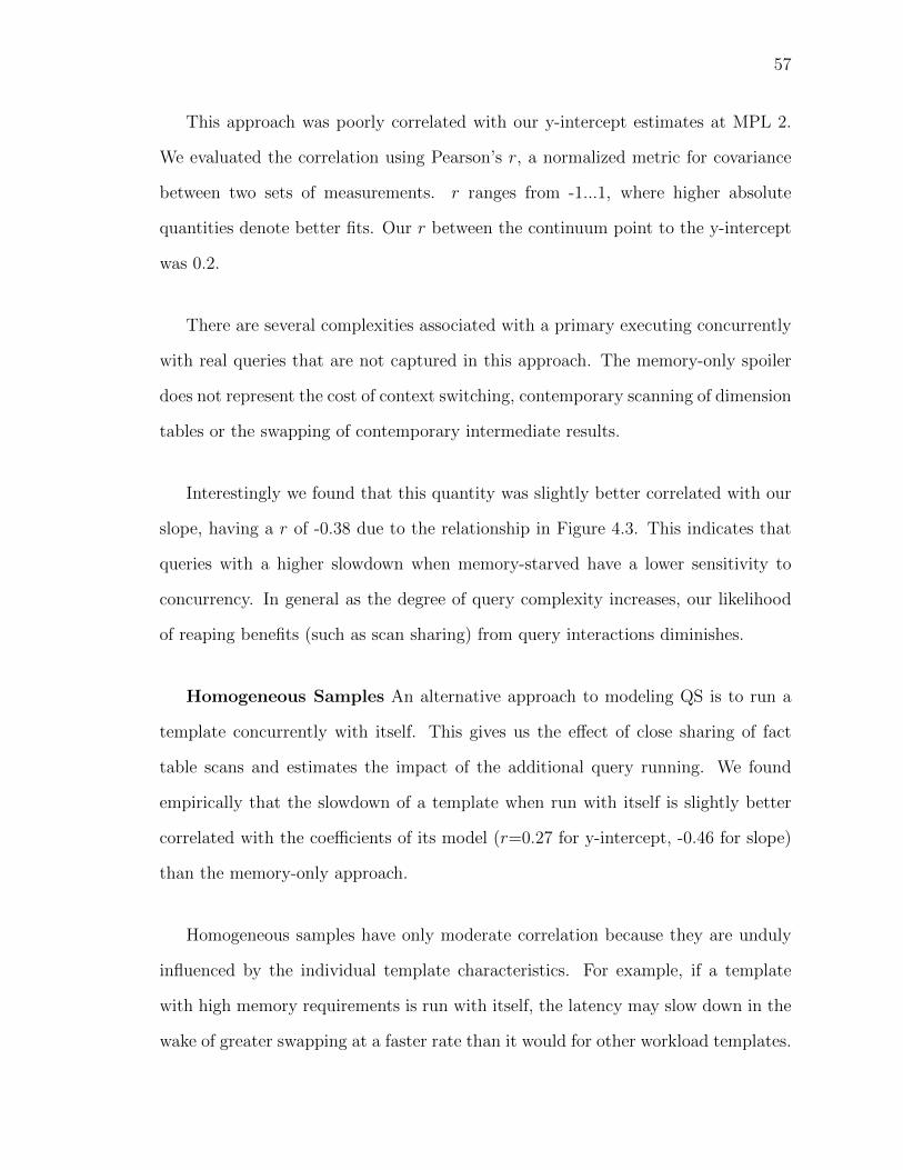
57
This approach was poorly correlated with our y-intercept estimates at MPL 2.
We evaluated the correlation using Pearson’s r, a normalized metric for covariance
between two sets of measurements. r ranges from -1...1, where higher absolute
quantities denote better fits. Our r between the continuum point to the y-intercept
was 0.2.
There are several complexities associated with a primary executing concurrently
with real queries that are not captured in this approach. The memory-only spoiler
does not represent the cost of context switching, contemporary scanning of dimension
tables or the swapping of contemporary intermediate results.
Interestingly we found that this quantity was slightly better correlated with our
slope, having a r of -0.38 due to the relationship in Figure 4.3. This indicates that
queries with a higher slowdown when memory-starved have a lower sensitivity to
concurrency. In general as the degree of query complexity increases, our likelihood
of reaping benefits (such as scan sharing) from query interactions diminishes.
Homogeneous Samples An alternative approach to modeling QS is to run a
template concurrently with itself. This gives us the effect of close sharing of fact
table scans and estimates the impact of the additional query running. We found
empirically that the slowdown of a template when run with itself is slightly better
correlated with the coefficients of its model (r=0.27 for y-intercept, -0.46 for slope)
than the memory-only approach.
Homogeneous samples have only moderate correlation because they are unduly
influenced by the individual template characteristics. For example, if a template
with high memory requirements is run with itself, the latency may slow down in the
wake of greater swapping at a faster rate than it would for other workload templates.

58
Y-Intercept Slopept 0.18 -0.05
Max Working Set -0.24 0.11Plan Nodes 0.31 -0.29
Records Accessed 0.12 -0.22Isolated Latency 0.36 -0.51Spoiler Latency 0.27 -0.49
Spoiler Slowdown 0.08 -0.24
Table 4.3: r between template traits and model coefficients at MPL 2.
While this did exhibit a better correlation to our y-intercept, it required executing
time-consuming additional sampling. This, like the memory-only spoiler, was an
unattractive way to learn our model parameters.
Template Properties Next we examined parameter estimation by looking for
trends in the query execution plan and resources used in our existing samples. By
looking at template properties, we could predict how a query would react to changing
I/O availability. We examined both performance features, such as percent I/O time
(pt) and maximum working set size, the size of the largest intermediate result in
our QEP. We also analyzed query complexity, by charting how closely the number
of plan nodes and records accessed correlated with our coefficients. Finally, we
evaluated the continuum itself, correlating the isolated run time, spoiler latency and
spoiler slowdown (by dividing spoiler latencies by the corresponding isolated query
duration). By looking at how a query “stretches” its latency, we may be able to
learn our models. Our findings are in Table 4.3.
Our performance features, pt and working set size, were poorly correlated with
our model parameters. This is not surprising because these parameters were too fine-
grained to summarize the query’s sensitivity to concurrency. Likewise, the number
of QEP nodes and records accessed also gave us too little information about overall
query behavior. Spoiler slowdown only conveyed the worst-case scenario, stripping

59
out valuable information regarding the query as a whole.
Isolated latency We found that isolated latency is inversely correlated with
slope in our model. Isolated latency is a useful approximation of the “weight” of a
query. Queries that are lighter weight tend to have larger slopes. They are more
sensitive to changing I/O availability and exhibit greater variance in their latency
under different concurrent mixes. In contrast, heavier queries (with high isolated
latencies) tend to be less perturbed by concurrency; their longer lifespans average out
brief concurrency-induced interruptions. Isolated latency is also positively correlated
with y-intercepts, due to the relationship in Figure 4.3. We learn from isolated
latency to predict Contender’s slopes for the remainder of this work.
Prediction pipeline for unseen templates
We build our prediction model in two phases (see Figure 4.4). First we train on a
known workload, drawing from isolated, spoiler and limited concurrent mix samples.
Next we use linear regression to estimate the slope, µt, based on our query’s isolated
latency. We learn this relationship based on other queries in our workload. Using
this estimated slope, we can learn the y-intercept, bt, using a second regression step.
We learn from a trend line such as that in Figure 4.3. This is step 3 in our framework.
By assembling these two estimated parameters, we can produce a prediction
of a new template t’s continuum point for an arbitrary mix. We do this by first
parsing the contemporary queries and estimating their I/O requirements (i.e., rci
values in Equation 4.4) and then calculate the CQI value for the template query t
(Equation 4.5). We then apply our estimated coefficients, µt and bt, to the CQI value
to estimate our continuum point based on the regression model in Equation 4.6.

60
!"#$%&'()*%&'+,-))))))))))).)))))
!"#$%$%&'
/0#1$'2)*%&'+,-))))))))))).)))
34)&'50$%&')
*%6+)7-0'2,89')/%50$'")
/%50$1+:)
;'<'2'+,')=#('$")2&>5)!),&>5)
34)?'50$%&'),&>5)@)5&2&>5)A)9&)
!
(lmin t )
!()*%&'
!
(lmin t )B%$,8$%&')BC!)D2&>5E)
B#+,822'+&)51F'")
!
(lmax t )
=#('$)G"65%))))!)H&>)9&)
!
lmin t
!"#$%&'()*%&'+,-))))))))))).)))))
?'50$%&'))=#('$)2&>5)!),&>5)
=%0)&#)$%&'+,-),&>5)!)$&>5)
*%&'+,-)02'(1,6#+)<#2)&'50$%&')!)1+)51F)"#
/0#1$'2)*%&'+,-))))))))))).)))
!
(lmax t )ID+E)"%50$1+:)#<)+'J)&'50$%&')!))
B#+,822'+&))51F)"#
3)
K)
L)M)
Figure 4.4: Process for predicting cQPP.
Given the continuum point, we use the isolated and spoiler latencies for the
template to scale it into a latency estimate, reversing Equation 4.1. Using this
technique, we can predict end-to-end latency for a new template as a part of arbitrary
mixes using just its isolated and spoiler latency samples.
4.3.3 Reduced Sampling Time
One of the appealing aspects of Contender is that it requires very limited sampling
to achieve high quality predictions. Specifically, we require only the spoiler latency
for each template paired with semantic information from its execution plan. This
is a very simple and flexible system for inserting new templates into pre-existing
workloads.
In prior work (e.g., [23]), the authors required significant sampling of new tem-
plates interacting with their workload before they can make predictions. This is
inflexible and causes an exponential growth in sampling requirements as the number
of distinct templates grow. This system used Latin Hypercube Sampling (LHS) in
its training phase for each template. For a workload with t templates with m MPLs
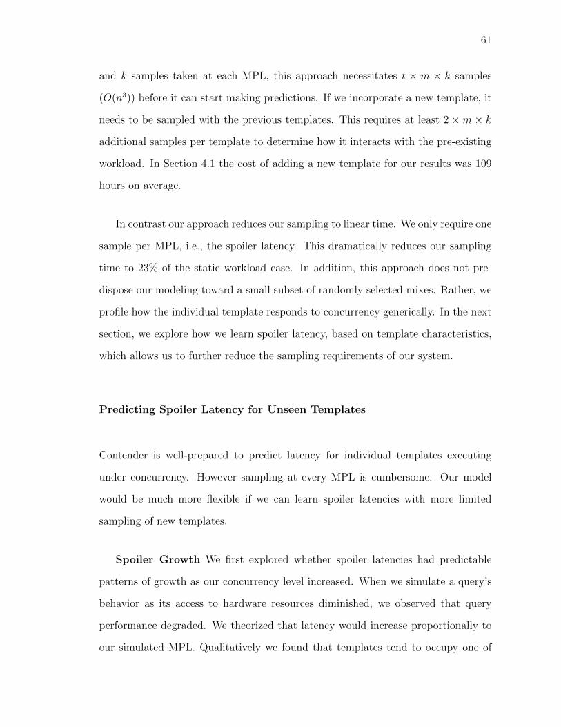
61
and k samples taken at each MPL, this approach necessitates t × m × k samples
(O(n3)) before it can start making predictions. If we incorporate a new template, it
needs to be sampled with the previous templates. This requires at least 2 ×m × k
additional samples per template to determine how it interacts with the pre-existing
workload. In Section 4.1 the cost of adding a new template for our results was 109
hours on average.
In contrast our approach reduces our sampling to linear time. We only require one
sample per MPL, i.e., the spoiler latency. This dramatically reduces our sampling
time to 23% of the static workload case. In addition, this approach does not pre-
dispose our modeling toward a small subset of randomly selected mixes. Rather, we
profile how the individual template responds to concurrency generically. In the next
section, we explore how we learn spoiler latency, based on template characteristics,
which allows us to further reduce the sampling requirements of our system.
Predicting Spoiler Latency for Unseen Templates
Contender is well-prepared to predict latency for individual templates executing
under concurrency. However sampling at every MPL is cumbersome. Our model
would be much more flexible if we can learn spoiler latencies with more limited
sampling of new templates.
Spoiler Growth We first explored whether spoiler latencies had predictable
patterns of growth as our concurrency level increased. When we simulate a query’s
behavior as its access to hardware resources diminished, we observed that query
performance degraded. We theorized that latency would increase proportionally to
our simulated MPL. Qualitatively we found that templates tend to occupy one of

62
!"
#!!!"
$!!!"
%!!!"
&!!!"
'!!!!"
'#!!!"
'$!!!"
'%!!!"
'&!!!"
'" #" (" $" )"
!"#$%&'()*$&*+(
,-./01231"445%3(!$6$.(
##"
%#"
*'"
Figure 4.5: Spoiler latency under increasing multiprogramming levels.
three categories. We have plotted one example of each in Figure 4.5.
The first category is demonstrated by Template 62. It is a very lightweight,
simple template. It has one fact table scan and very small intermediate results. This
query is subject to slow growth as contention increases as it is not strictly I/O bound.
In isolation it uses 87% of the I/O bandwidth.
Our second medium weight category is shown with Template 71. It is I/O bound
using greater than 99% of the I/O bandwidth in isolation. However, it does not have
large intermediate results. Because of these two factors, it exhibits modest linear
growth as we increase the MPL.
The final type of queries in our workload are heavy. These queries are shaped
by large intermediate results which necessitate swapping as our degree of contention
increases. They have a much higher slope. These templates exhibit linear increases
in latency, however their growth rate is much faster than that of the other two classes.
All of these responses exhibit linear growth, albeit different rates. By learning
from the first m spoiler latencies, where m is our multiprogramming level, we can
build a pattern for each template to estimate our upper bound at higher levels of

63
pt WS Size Rand. I/Or2 0.63 0.41 0.00
Table 4.4: Correlation between I/O profile components and spoiler models.
contention. Logically query latency should grow in proportion to the simulated MPL.
We experimented with training a linear regression model for each template. We
learned from MPLs 1-3 and evaluated our models on MPLs 4-5. We found that on
average we could predict spoiler latency within 8% of the correct elapsed time using
this technique. This demonstrates that there is a simple linear relationship between
query performance and simulated MPL.
Learning Spoiler Growth Patterns We have demonstrated that spoiler per-
formance for individual templates grows linearly proportional to our simulated MPL.
As detailed in Figure 4.5, individual templates have very different latency growth
rates as our simulated MPL increases. However we can estimate the slope for each
template by evaluating how comparable they are to other templates in our workload.
To this end we first normalize our spoiler latencies. For each spoiler recording we
divide by a template’s isolated performance so that our predictions revolve around
spoiler slowdown rather than latency.
We now turn our attention to predicting the coefficients for these models. To
predict a template’s response to the spoiler, we develop a profile of its I/O behavior.
We begin with three metrics for to describe query performance in isolation: pt, work-
ing set size and percent of time spent executing random I/O. In [26] the researchers
have predicted latency as well as I/O-level metrics for queries executing in isolation.
In future work we could leverage this to predict our template profiles.
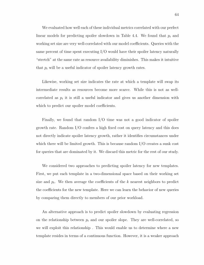
64
We evaluated how well each of these individual metrics correlated with our perfect
linear models for predicting spoiler slowdown in Table 4.4. We found that pt and
working set size are very well-correlated with our model coefficients. Queries with the
same percent of time spent executing I/O would have their spoiler latency naturally
“stretch” at the same rate as resource availability diminishes. This makes it intuitive
that pt will be a useful indicator of spoiler latency growth rates.
Likewise, working set size indicates the rate at which a template will swap its
intermediate results as resources become more scarce. While this is not as well-
correlated as pt it is still a useful indicator and gives us another dimension with
which to predict our spoiler model coefficients.
Finally, we found that random I/O time was not a good indicator of spoiler
growth rate. Random I/O confers a high fixed cost on query latency and this does
not directly indicate spoiler latency growth, rather it identifies circumstances under
which there will be limited growth. This is because random I/O creates a sunk cost
for queries that are dominated by it. We discard this metric for the rest of our study.
We considered two approaches to predicting spoiler latency for new templates.
First, we put each template in a two-dimensional space based on their working set
size and pt. We then average the coefficients of the k nearest neighbors to predict
the coefficients for the new template. Here we can learn the behavior of new queries
by comparing them directly to members of our prior workload.
An alternative approach is to predict spoiler slowdown by evaluating regression
on the relationship between pt and our spoiler slope. They are well-correlated, so
we will exploit this relationship . This would enable us to determine where a new
template resides in terms of a continuous function. However, it is a weaker approach

65
because it necessitates using just one of our indicators.

Chapter Five
Bringing Workload Performance
Prediction to Portable Databases

67
!""#$
!"""#$
!""""#$
%&'()*$ +,-.&$ /+,-.&$ 0(.1$234$
!"#$%&"
'#()"%*++,+%
-./%0$12#$3"%
Figure 5.1: Fine grained regression for workload throughput prediction on Amazon Web Servicesinstances using TPC-DS.
5.1 Fine Grained Profiling
In the section, we demonstrate that a simple, query-at-a-time modeling approach
poorly predicts throughput for portable databases. This finding underlines the need
for a more general profiling solution. In this approach, we create a model for each
platform based on aggregating over its member queries. Our goal was to see if by
analyzing the resource requirements of individual queries in our workload, we could
build a model to describe how they would perform as a collection. By summing up
how the member queries used resources, we could quantify the total strain on our
system.
In theory this approach should be promising. We build a profile of each workload
where we sum up the strain that the member queries would place on the system
if executed in isolation. This should indicate the rate at which our workload can
make progress and hence predict throughput. However we found that in practice
this approach fails to capture the lower level interactions among our queries. We
cannot model savings from beneficial relationships such as shared scans. We also
fail to capture slowdown, such as two memory-intensive queries creating expensive
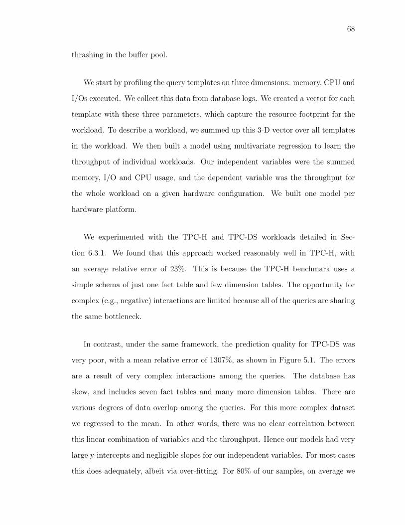
68
thrashing in the buffer pool.
We start by profiling the query templates on three dimensions: memory, CPU and
I/Os executed. We collect this data from database logs. We created a vector for each
template with these three parameters, which capture the resource footprint for the
workload. To describe a workload, we summed up this 3-D vector over all templates
in the workload. We then built a model using multivariate regression to learn the
throughput of individual workloads. Our independent variables were the summed
memory, I/O and CPU usage, and the dependent variable was the throughput for
the whole workload on a given hardware configuration. We built one model per
hardware platform.
We experimented with the TPC-H and TPC-DS workloads detailed in Sec-
tion 6.3.1. We found that this approach worked reasonably well in TPC-H, with
an average relative error of 23%. This is because the TPC-H benchmark uses a
simple schema of just one fact table and few dimension tables. The opportunity for
complex (e.g., negative) interactions are limited because all of the queries are sharing
the same bottleneck.
In contrast, under the same framework, the prediction quality for TPC-DS was
very poor, with a mean relative error of 1307%, as shown in Figure 5.1. The errors
are a result of very complex interactions among the queries. The database has
skew, and includes seven fact tables and many more dimension tables. There are
various degrees of data overlap among the queries. For this more complex dataset
we regressed to the mean. In other words, there was no clear correlation between
this linear combination of variables and the throughput. Hence our models had very
large y-intercepts and negligible slopes for our independent variables. For most cases
this does adequately, albeit via over-fitting. For 80% of our samples, on average we
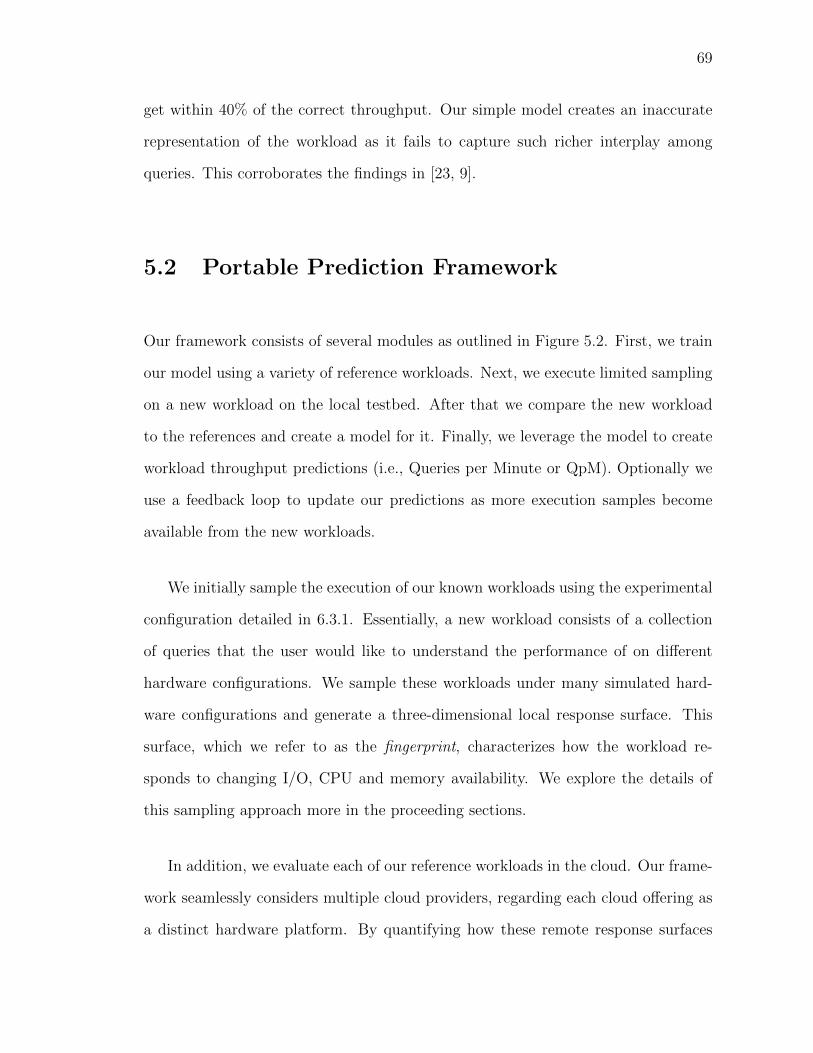
69
get within 40% of the correct throughput. Our simple model creates an inaccurate
representation of the workload as it fails to capture such richer interplay among
queries. This corroborates the findings in [23, 9].
5.2 Portable Prediction Framework
Our framework consists of several modules as outlined in Figure 5.2. First, we train
our model using a variety of reference workloads. Next, we execute limited sampling
on a new workload on the local testbed. After that we compare the new workload
to the references and create a model for it. Finally, we leverage the model to create
workload throughput predictions (i.e., Queries per Minute or QpM). Optionally we
use a feedback loop to update our predictions as more execution samples become
available from the new workloads.
We initially sample the execution of our known workloads using the experimental
configuration detailed in 6.3.1. Essentially, a new workload consists of a collection
of queries that the user would like to understand the performance of on different
hardware configurations. We sample these workloads under many simulated hard-
ware configurations and generate a three-dimensional local response surface. This
surface, which we refer to as the fingerprint, characterizes how the workload re-
sponds to changing I/O, CPU and memory availability. We explore the details of
this sampling approach more in the proceeding sections.
In addition, we evaluate each of our reference workloads in the cloud. Our frame-
work seamlessly considers multiple cloud providers, regarding each cloud offering as
a distinct hardware platform. By quantifying how these remote response surfaces

70
!"#$%&'(#)*%+(&
,&
-./0"+&(+1+(+23+&4#(5"#.%6&&"#3.""7&.2%&*2&89+&3"#$%&
Model building
'+(1#(/.23+&&'(+%*3:#26&
-./0"+&2+4&4#(5"#.%6&"#3.""7&
!"#$%&4#(5"#.%&
;&
!"#$%&'(#)*%+(&
;&
<23(+/+28.""7&*/0(#)+&89+&&0(+%*3:#26&=7&*23#(0#(.:2>&1++%=.35&&1(#/&89+&3"#$%&
?&
;&
,&
@&
Figure 5.2: System for modeling and predicting workload throughput.
varied, we determined common behavioral patterns for analytical workloads in the
cloud. We learn from our reference workloads’ performance in the cloud rather than
interpolating within the local testbed. This makes us robust to hardware platforms
that exceed our local capacity.
Next we sample new workloads that are disjoint from the training set. We locally
simulate a representative set of hardware configurations for the new workloads by
creating local response surface. Finally we create predictions for new workloads
on remote platforms by comparing their response surface to that of the reference
workloads. We present the details of this process in Section 5.4.
In addition we incrementally improve our model for new workloads by adding in-
cloud performance to its fingerprint. As we refine our fingerprint for the workload,
we create higher quality predictions for new, unsampled platforms.
5.3 Local Response Surface Construction
In our design, we create a simple framework for simulating hardware configurations
for each workload using a local testbed. When we evaluate our new queries locally
we obviate the noisiness that may be caused by virtualization and multi-tenancy.

71
Although we did not empirically find these complexities to be a significant factor, a
local testbed allows us to control for them.
We call our hardware simulation system a spoiler because it occupies resources
that would otherwise be available to the workload.1 The spoiler manipulates resource
availability on three dimensions: CPU time, I/O bandwidth and memory. We con-
sider the local response surface to be an inexpensive surrogate for cloud performance.
We experiment with a workload by slicing this three dimensional response surface
along several planes. In doing so, we identify the resources upon which the workload
is most reliant. Not surprisingly, the I/O bandwidth was the dominant factor in
many cases, followed by the memory availability.
We control the memory dimension by selectively taking away portions of our
RAM. We did this by allocating the space in the spoiler and pinning it in memory.
This forced the query to swap if it needed more than the available RAM. In our case
we start with 4 gigabytes of memory and increment in steps of four until we reach
our maximum of 16 gigabytes.
We regulate the CPU dimension by taking a percent of the CPU to make available
to the database. For simplicity we set our number of cores equal to our multipro-
gramming level. Hence each query had access to a single core. We simulated our
system having access to 25%, 50%, 75% and 100% of the CPU time. We did this by
making a top priority process that executes a large number of floating point opera-
tions. We time the duration of the arithmetic and sleep for the appropriate ratio of
CPU time.
1We derive its name from the American colloquialism “something that is produced to competewith something else and make it less successful.”

72
46
810
1214
16
0.5
1
1.5
2
2.51
2
3
4
5
6
7
Memory (GB)CPU (GHz)Q
pMFigure 5.3: Local response surface for a TPC-DS workload with high I/O availability. Responsesare in queries per minute. Low I/O dimension not shown.
We had a coarse-grained metric for I/O availability: low or high. Most cloud
providers have few levels of quality of service for their I/O time. To the best of
our knowledge Amazon Elastic Block Store is the only service that allows users to
provision I/Os per second and this is a premium option. We simulated this by
making our high availability give the database unimpeded access to I/O bandwidth.
For the low I/O bandwidth case we had a competing process that circularly scanned
a very large file at equal priority to the workload.
An example local response surface is depicted in Figure 5.3. We see that its
throughput varies from zero to seven QpM. This workload’s throughput exhibits a
strong correlation with memory availability. Most contention was in the I/O sub-
system both through scanning tables and through swapping intermediate results as
memory becomes less plentiful.
5.4 Model Building
We elected to use a prediction framework inspired by memory-based version of col-
laborative filtering [31] to model our workloads. This approach is typically used in
73
recommender systems. In simplified terms, collaborative filtering identifies similar
objects, compares them and makes predictions about their future behavior. This
part of our framework is labelled as “model building” in Figure 5.2.
One popular application for collaborative filtering is movie recommendations,
which we shortly review as an analogous exercise. When a viewer v asks for a movie
recommendation from a site such as Netflix, the service would first try to identify
similar users. It would then average the scores that similar viewers had for movies
that v has not seen yet to project ratings for v. It can then rank the projected
ratings and return the top-k to v.
In our case, we forecast QpM for a new workload. We compute the similarity for
our new workload to that of our references. We then calculate a weighted average
of their outcomes for the target cloud platform based on similarity. We found that
by using these simple steps, we could achieve high quality predictions with little
training on new workloads.
Our implementation first normalizes each reference workload to make it compa-
rable to others. We zero mean its throughputs and divide by the standard deviation.
This enables us to account for different workloads having distinct scales in QpM. For
each reference workload r and hardware configuration h, we have a throughput tr,h.
We have an average throughput of ar and a standard deviation σr. We normalize
each throughput as:
tr,h =tr,h − arσr
This puts our throughputs on a scale of approximately -1...1. We apply this
Gaussian normalization once per workload. This makes one workload comparable to
the others.

74
When we receive a new workload i, for which we are creating a prediction, we
normalize it similarly and then compare it to all of our reference workloads. For i we
have samples of it executing on a set of hardware configurations Hi. We discuss our
sampling strategies in the next section. For each pair of workloads i, j we compute
Si,j = Hi ∩Hj or the hardware configurations on which both have executed. We can
then estimate the similarity between i and j as:
wi,j =1
|Si,j|∑h∈Si,j
ti,htj,h
After that we forecast the workload’s QpM on a new hardware platform, h, by taking
a similarity-based weighted average of their normalized throughputs:
ti,h =
∑j|Si,j 6=∅,h∈Hj
wi,jtj,h∑j|Si,j 6=∅,h∈Hj
|wi,j|
This forecasting favors workloads that most closely resemble the one for which we
are creating a prediction. We downplay those that are less relevant to our forecasts.
Naturally we can only take this weighted average for the workloads that have
trained on h, the platform we are modeling. We can create predictions for both
local and in-cloud platforms using this technique. While we benefit if our local test
bed physically has more resources than the cloud-based platforms upon which we
predict, we can use the model for cloud platforms exceeding our local capabilities.
The only requirement for us to create a prediction is that we have data capturing how
training workloads respond to each remote platform. Experimentally we evaluate
cloud platforms that are both greater and less than our local testbed in hardware
capacity.

75
Query 1 2 3 4 51 X2 X3 X4 X5 X
Figure 5.4: An example of 2-D Latin hypercube sampling.
We then derive the unnormalized throughput as:
ti,h = ti,hσi + ai
This is our final prediction.
5.5 Sampling
We experimented with two sampling strategies for exploring a workload’s response
surface. We first consider Latin hypercube sampling, a technique that randomly
selects a subsection of the available space with predictable distributions. We also
evaluate adaptive sampling, in which we recursively subdivide the space to charac-
terize the novel parts of the response surface.
Latin Hypercube Sampling Latin hypercube sampling is a popular way to
characterize a surface by taking random samples from it. It was used in [23, 5] for
a static hardware variant of this problem. It takes samples such that each plane in
our space is intersected exactly once, as depicted in Figure 5.4.
In the complete version of Figure 5.3, we first partition the response surface by
I/O bandwidth, a dimension that has exactly two values for our configuration. We

76
do this such that our dimensions are all of uniform size to adhere to the requirement
that each plane is sampled exactly once. We then have two 4x4 planes and we sample
each four times at random.
Adaptive Sampling We submit that our local response surface is monotonic.
This is intuitive; the more resources a workload has, the faster it will complete.
To build a collaborative filtering model we need to determine its distribution of
throughputs. Exhaustively evaluating this continuous surface is not practical. On
average it would take us 88 hours to analyze a single workload if we did so in a coarse
grid.
We also considered using a system such as [22], in which the authors explore a high
dimensional surface of database configurations. They identify regions of uncertainty
and sample the ones that are most likely to improve their model. However this
technique is likely to evaluate more than is necessary because it presumes a non-
monotonic surface. By exploiting the clear relationship between hardware capacity
and performance, we may reduce our sampling requirements.
Hence we propose an adaptive sampling of the space. We start by sampling the
extreme points of our local response surface. This corresponds to (2.4 GHz, 16 GB,
High) and (0.6 GHz,4 GB, Low) in the full version of Figure 5.3. We first test to
see if the range established by these points is significant. If it is very small, then
we stop. Otherwise we recursively subdivide the space until we have a well-defined
model.
We subdivide the space until we observe that the change in throughput is ≤n%
of the response surface range. Our recursive exploration of the space first divides
the response surface by I/O bandwidth. We do this because I/O bandwidth is the
77
!"# !$# !%# !"# !$# !%#
!%# !"# !$# !%# !"# !$# !%#
!$# !%# !"# !$# !%# !"#
&'#
&(#
&)#
*+,-#
Figure 5.5: Example workload for throughput evaluation with three streams with a workload ofa, b, and c.
dimension most strongly correlated with throughput. After that we subdivide on
memory availability. It too directly impacts the I/O bottleneck. Finally we sample
among changing CPU resources if we have not reached a stopping condition.
5.6 Preliminary Results
In this section, we first detail our experimental configurations. We then explore the
cloud response surface, for which we are building our models. Next, we evaluate the
effectiveness of our prediction framework for cloud performance based on complete
sampling of the local response grid. After that, we investigate how our system
performs with our two sampling strategies. Finally, we look at the efficacy of our
models gaining feedback from cloud sampling.
5.6.1 Experimental Configuration
We experimented with TPC-DS and TPC-H, two popular analytical benchmarks at
scale factor 10. We evaluated using all but the 5 longest running queries on TPC-
H and using 74 of the 100 TPC-DS templates, again omitting the longest running
ones. We did not use the TPC-DS templates that ran for greater than 5 minutes in
isolation on our highest local hardware configuration. We elected to omit the longest

78
running queries because under concurrency their execution times grow very rapidly
and we kept the scope of our experiments to 24 hours or less each. Nonetheless
a portion of our experiments (2%) still exhibited unbounded latency growth. We
terminated them after 24 hours and record them as having zero QpM.
We implemented a variant of the TPC-H throughput test. An example of our
setup is displayed in Figure 6.12. Specifically we created a workload with 5 templates,
± 1 to account for modulus cases. Our trials were all at multiprogramming level 3,
in accordance with TPC-H standards. Each of our three query streams executed a
permutation of the workload’s templates. We executed at least 5 examples of each
stream before we concluded our test. We omit the first and last few queries from
each experiment to account for a warmup and cool down time. We compute the
queries per minute (QpM) for the duration of the experiment.
We created 23 TPC-DS workloads using this method. The first 8 were configured
to look at increasing database sizes. The first two access tables totaling to 5 GB,
the second two at 10 GB, et cetera. The remaining 15 workloads were randomly
generated without replacement. For TPC-H we randomly generated 9 workloads.
There were three sets of three permutations without replacement.
We quantify the quality of our predictions using mean relative error as in [23,
9, 5]. We compute it for each prediction as |observed−predicted|observed
. This metric scales our
predictions by the throughputs, giving an intuitive yardstick for our errors.
For our in-cloud evaluations we used Amazon EC2 and Rackspace. We rented
EC2’s m1.medium, m1.large, m1.xlarge and hi1.4xlarge instances. The first three are
general purpose virtual machines at increasing scale of hardware. The final is an I/O
intensive SSD offering. We considered experimenting on their micro instances and
79
conducted some experiments on AWS’s m1.small offering. However we found that so
many of our workloads do not complete within our time requirement in this limited
setting that we ceased pursuing this option. When a workload greatly outstrips the
hardware resources available it is reduced to thrashing as it swaps continuously. In
Rackspace we experimented on their 4, 8, 16, and 32 GB cloud offerings.
We used k-fold cross validation (k=4) for all of our trials. That is, we partition
our workloads into k equally sized folds, train on k−1 folds and test on the remaining
one.
5.6.2 In Cloud Performance
In Figure 6.13 we detail the throughput for our individual workloads as they are
deployed on a variety of cloud instances. We see a monotonic surface much like the
ones that we encounter with the local testbed. This indicates that there may be
exploitable correlations between the two surfaces.
For TPC-H we see that the majority of our workloads are of moderate intensity.
They have a gradual increase in performance until they reach the extra large instance.
At that point many of the workloads fit in the 7.5 GB of memory, seeing only modest
gains from the largest instance. There are three workloads that are more intensive
(shown in dashed lines). They have greater hardware requirements and do not see
performance gains until the database is completely memory resident.
TPC-DS has a more diverse response to the cloud offerings. The majority follow
a curve similar to that of TPC-H. There is one that never achieves performance
gains because it is entirely CPU bound. We also have two examples of the memory-

80
!"
#"
$"
%"
&"
'"
("
)"
*"
+"
,-./01" 2345-" 67345-" 8/59":;<"
!"#
$%#&'(')
%*"+#'
,-.'/*&+0*1#'
!"
$"
&"
("
*"
#!"
#$"
#&"
#("
#*"
,-./01" 2345-" 67345-" 8/59":;<"
!"#
$%#&'(')
%*"+#'
,-.'/*&+0*1#'
=3>" =?>"
Figure 5.6: Cloud response surface for (a) TPC-H and (b) TPC-DS
intensive “knee” as seen in TPC-H, again as a dashed line. The consistency of the
response surfaces also indicates that our cloud evaluation was robust to noisiness
that is a part of the multi-tenant cloud environment.
Next we examine the quality of our predictions for a new workload if we have
very good knowledge of its local response surface. For each workload we sampled
the entire grid in Figure 5.3 locally. Our prediction results are in Figure 6.14. We
observed that the quality of our predictions steadily increased for TPC-DS with our
provisioned hardware. As the workloads had more resources they thrash and swap
less. This makes their outcomes more predictable.
In contrast our predictions in TPC-H get slightly worse for the larger instances.
This is a side effect of the three dashed workloads that are memory-intensive. They
exhibit limited growth in the smaller instances and have a dramatic take off when
they have sufficient RAM. This is an under-sampled condition. If we omit them from
our calculations, our average error drops to 20% for the highest two instances.
It is interesting to see that these two response surfaces in Figure 6.13 are very
comparable despite their different schemas. This demonstrates that both analytical
benchmarks are highly I/O bound and that we have fertile ground to learn across
databases rather than having to deploy a new database in the cloud before we can

81
!"#
$"#
%!"#
%$"#
&!"#
&$"#
'!"#
'$"#
(!"#
)*+# ,-./01# 234+-# 5634+-# 7/+8#9:;#
!"#$%&"
'#()"%*++,+%
-./%0$12#$3"%
<=>?@A#
<=>?7#
Figure 5.7: Prediction errors for cloud offerings.
make predictions.
5.6.3 Cross Schema Prediction
We found that we could predict TPC-DS based on TPC-H only training within 27%
of the correct throughput on average. The results showed encouraging evidence that
the framework can successfully identify the important similarities across workloads
that are drawn from different set of queries and schemas.
5.6.4 Sampling
Next we quantify the speed at which adaptive sampling converged on a response
surface. We configured our algorithm such that if the range is less than 1 QpM
we cease sampling. We made our stopping condition for recursion 33% of the range
established by the initial, most distant points. We found that on average we sampled
43% of the space for TPC-DS and 33% for TPC-H.
This is a very high sampling rate, considering that our local trials take 165

82
!"#
$!"#
%!"#
&!"#
'!"#
(!"#
)!"#
*!"#
+!"#
,!"#
-./# 012345# 678/1# 9:78/1# ;3/<#=>?#
!"#$%&"
'#()"%*++,+%
-./%0$12#$3"%
67AB#;C@18D4E1#
F832#
Figure 5.8: Prediction errors for each sampling strategy in TPC-H.
minutes on average. This would mean that for TPC-DS we would have to conduct
38 hours worth of experiments before we could predict on the cloud. This is a very
high cost and perhaps not a practical use case. We also noticed that there is a high
degree of variance in the number of points we sampled per response surface. The
standard deviation for our number of points sampled was 5.5 trials for TPC-DS,
demonstrating noticeable unpredictability in our sampling times.
Adaptive sampling displayed an impedance mismatch with our prediction model.
The collaborative filtering model required a set of samples that is representative of
the data both in terms of its distinct values and their frequency. Adaptive sampling
captures their distinct values more precisely, but fails to observe their frequency.
This distorts the normalization phase and hence our predictions.
For our Latin hypercube sampling trials we sampled 8 points or 25% of the local
response surface. While this sampling is robust, it is considerably less costly than the
adaptive alternative. By spacing our random samples such that they all intersect
each distinct dimension value once we achieve a more representative view of the
space.
We evaluate the accuracy of our predictions using different sampling techniques

83
in Figure 6.15. We see that adaptive sampling does very poorly in comparison to the
full grid and Latin hypercube approaches. This is because we oversample the spaces
that exhibit rapid change and do not give due weight to the ones that are more stable
and likely to be the average case. In future work we could mitigate this limitation by
interpolating the response surface based on known points. Latin hypercube sampling
demonstrates prediction accuracy on par with that of grid sampling, showing that
this approach is well-matched to our prediction engine. We do perform slightly better
in the m1.large case. This is a 2% difference is a negligible noise due to the spoiler
simulations.
In Figure 6.16 we compare (1) our TPC-DS predictions on Rackspace with
Latin hypercube sampling to (2) those that are based on LHS and incorporating
m1.medium and m1.xlarge samples from our AWS experiments. For the LHS-only
sampling case we found that it was slightly harder to predict than in Amazon AWS.
The response surfaces on Rackspace were slightly less smooth than AWS, implying
that multi-tenancy may have been playing a larger role in this environment.
In the second series (shown as Local LHS+AWS), we evaluated how augmenting
our models with cloud samples would improve our predictions. We found that this
feedback modestly but appreciably increased our accuracy. This demonstrated that
our incremental improvement of the model benefits from the feedback and that cross-
cloud knowledge is portable.
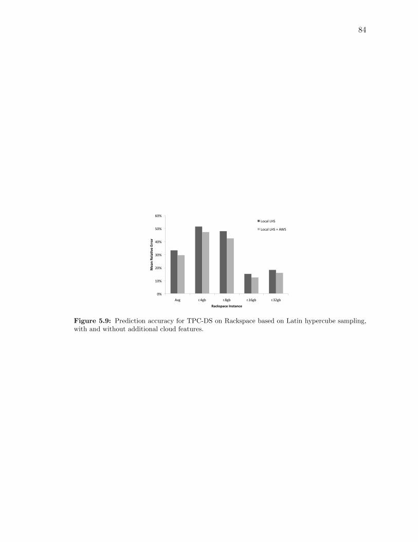
84
!"#
$!"#
%!"#
&!"#
'!"#
(!"#
)!"#
*+,# -.',/# -.0,/# -.$),/# -.&%,/#
!"#$%&"
'#()"%*++,+%
&#-./0#-"%1$/2#$-"%
12345#167#
12345#167#8#*97#
Figure 5.9: Prediction accuracy for TPC-DS on Rackspace based on Latin hypercube sampling,with and without additional cloud features.
Chapter Six
Experimental Evaluation
86
In this section we will first examine the effectiveness of the BAL and B2cB system.
After that we will examine how well Contender predicts cQPP in a more general-
ized setting. Finally we will review some preliminary results for portable workload
performance prediction.
6.1 B2L and B2cB
In this section we set out to verify the accuracy and utility of the four modules in
our framework. First we look at the accuracy of B2L, or how well our experiment-
driven model can use buffer access latency to predict end-to-end query latency under
varying concurrency levels and query mixes. Next, we examine how well our B2cB
model can predict BAL for use with B2L. After that we explore the accuracy of
combining these two techniques to produce end-to-end latency estimates. Finally,
we experiment with creating prediction on random, dynamically generated workloads
at a fixed multiprogramming level using our JIT and queue modeler timeline analysis
techniques.
We gathered data in two phases for our steady state experiments. Initially, we
create our training data consisting of several steady state mixes. Our training set
draws from samples at multiprogramming levels 1-5. Using the training data set
we build our prediction models for the concurrent buffer access latency (B2cB) and
the end-to-end latency (B2L). The details of this training process are in Section
3.2.1. B2cB produces coefficients for the multivariate prediction model for each
multiprogramming level. B2L produces its simple linear model for each query class.
Next we looked at a test data set, consisting of randomly selected mixes that are

87
disjoint from the training data. Our test data set is drawn from two Latin hypercube
sample sets per multiprogramming level, producing 20 steady state measurements.
Each steady state measurement is comprised of at least 5 queries per template in
the mix.
Finally, we experimented with completely arbitrary mixes, relaxing our steady
state assumption. This allowed us to evaluate our timeline analysis. Here we looked
at both incremental re-evaluation of our predictions (JIT) as well as creating only
one prediction when each query started (queue modeler).
6.1.1 Experimental Configuration
We experimented with a TPC-H query workload consisting of moderate weight
queries that exert strain on different parts of the database system. We targeted
OLAP because the queries are longer running, giving us a more time to characterize
their interactions. Analytical queries tend to be more highly I/O-bound, allowing
us to focus on this element for our interaction modeling rather than a more complex
multidimensional model that would have to take into account CPU slicing and other
resource sharing.
We worked with a mix of ten moderate weight queries. Specifically, our workload
is comprised of TPC-H queries 3, 4, 5, 6, 7, 8, 10, 14, 18 and 19 on an instance of TPC-
H, scale factor 10. We selected the ten queries on and around the median execution
time for all of the TPC-H templates. We focus on medium-weight queries because
they are long running enough such that we can make useful inferences about their
behavior. They are also light enough to allow for us to experiment with meaningful
multiprogramming levels.

88
Furthermore, we wanted to predict realistic workloads. We study concurrent
query mixes of different multiprogramming levels, however we do not address pre-
dictions for cases of very high contention. Therefore, we do not consider cases where
it is likely that a mix of queries could complete all of their executions in isolation
faster than running its queries concurrently.
We also elected to focus on moderate-weight queries because modeling across
multiple query weights adds another layer to the problem as demonstrated in [26].
In this work they classified their queries according to a relative weight and built
models for each group. In future work, we may extend our framework with a similar
labeling strategy.
In our experimental configuration we added the primary key indexes provided by
the standard TPC-H implementation. The benchmark was deployed on a modified
version of PostgreSQL 8.4.3. The source code was instrumented to measure BAL.
All of our trials were run on a machine with an Intel i7 2.8 GHz processors and 8
GB of RAM. The machine ran on Ubuntu 9.04 on Linux 2.6.28-11.
6.1.2 Predicting Query Contention
In this section we will look at how well our B2cB and B2L system can predict BAL
and end-to-end latency. All of the results below are evaluated on our test data,
disjoint from the training samples.

89
!"
#!!"
$!!"
%!!"
&!!"
'!!"
(!!"
)!!"
*!!"
+!!"
!" '!" #!!" #'!" $!!" $'!" %!!" %'!" &!!"
!"#$%&$'()*+$,-.(/#$-#0(
!"#$%&$'(12)(/3#0(
,%"
,&"
,'"
,("
,)"
,*"
,#!"
,#&"
,#*"
,#+"
Figure 6.1: Fit of B2L to steady state data at multiprogramming levels 3-5.
B2L
First we examine the effectiveness of B2L for estimating latency based on a pro-
vided BAL. We built our linear models for each query class on our training set at
multiprogramming levels 1-5. Our training phase produces simple equations of the
form
L = Oα + Pα ∗Bα (6.1)
for each query class in our workload.
We demonstrate the fit of our model with Figure 6.1. The points on this graph
are all from individual queries of our test data set with concurrency levels 3-5. The
lines denote the slope of an individual B2L model. Each query class fits very well
with its regression model. Our evaluation data produced an average error of just
5%. This tight fit is because queries generally will have latency proportional to the
rate at which they can access physical pages. This shows that despite relatively few
mixes sampled and varying concurrency levels, buffer access latency is an efficient
and robust estimator of query latency. To reiterate, none of the points evaluated
here were a part of the training phase.

90
It is clear that our B2L models fall into two main trajectories. These different
slopes are a consequence of our query templates having different query execution
plan layouts. Query plans can be divided into processing pipelines. These pipelines
delineate points in the query execution where results from the previous pipeline must
be completed before the next phase of a query may start. For example, sorts require
access to all of the tuples in their operation and thus require that executor start a
new pipeline for them (separate from the operators that provided tuples to the sort).
In future work, we may consider breaking our predictions down to the granularity of
pipelines as was done for progress estimators in [17].
The queries with smaller latency growth (queries 6, 14 and 19) had a single
pipeline (i.e., no materialization points such as sorts or group-by aggregates). The
remaining query classes which demonstrated a faster latency increase in proportion
to their BAL generally had greater than one pipeline in their query plans. This
means that the overall growth rate for each BAL is higher, due to the overhead of
the tuples having to traverse multiple pipelines and typically be evaluated by more
operators in the query plan.
B2cB
Now that we have established that average BAL is a good predictor of latency in the
case of varying resource contention, we turn to evaluating how well we can predict
this metric. We examine the accuracy of the B2cB approach for predicting average
BAL on the test data set.
The fit of B2cB predictions to measured BAL at multiprogramming level 3 in is
displayed in Figure 6.2. This charts all of the queries in the test mixes in steady
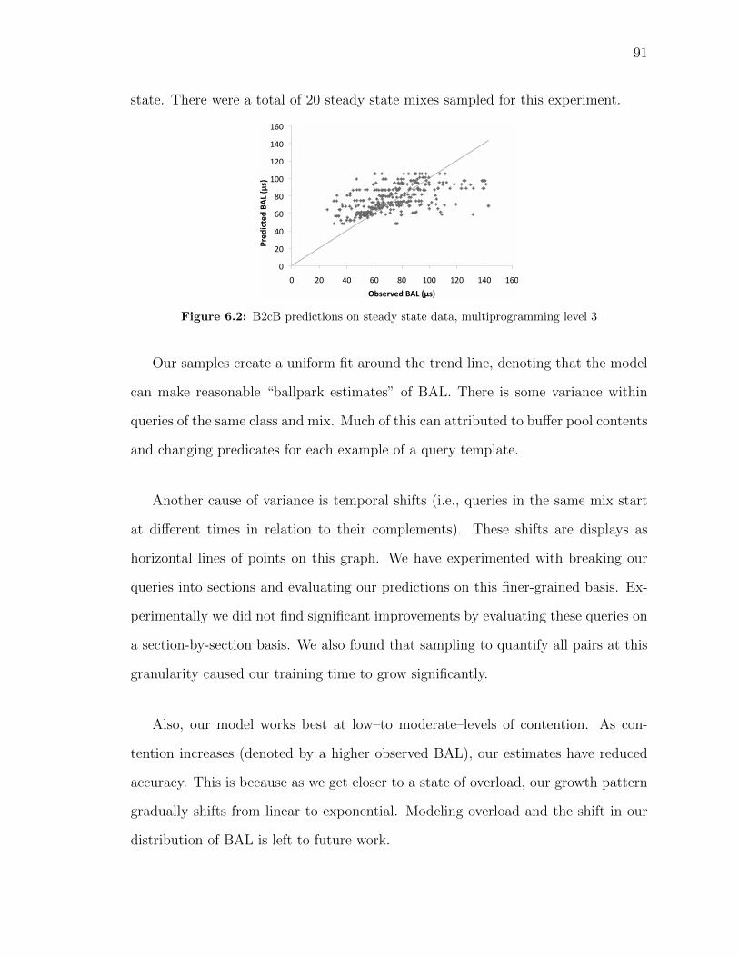
91
state. There were a total of 20 steady state mixes sampled for this experiment.
!"
#!"
$!"
%!"
&!"
'!!"
'#!"
'$!"
'%!"
!" #!" $!" %!" &!" '!!" '#!" '$!" '%!"
!"#$%&'#$()*+(,-./(
01.#"2#$()*+(,-./(
Figure 6.2: B2cB predictions on steady state data, multiprogramming level 3
Our samples create a uniform fit around the trend line, denoting that the model
can make reasonable “ballpark estimates” of BAL. There is some variance within
queries of the same class and mix. Much of this can attributed to buffer pool contents
and changing predicates for each example of a query template.
Another cause of variance is temporal shifts (i.e., queries in the same mix start
at different times in relation to their complements). These shifts are displays as
horizontal lines of points on this graph. We have experimented with breaking our
queries into sections and evaluating our predictions on this finer-grained basis. Ex-
perimentally we did not find significant improvements by evaluating these queries on
a section-by-section basis. We also found that sampling to quantify all pairs at this
granularity caused our training time to grow significantly.
Also, our model works best at low–to moderate–levels of contention. As con-
tention increases (denoted by a higher observed BAL), our estimates have reduced
accuracy. This is because as we get closer to a state of overload, our growth pattern
gradually shifts from linear to exponential. Modeling overload and the shift in our
distribution of BAL is left to future work.

92
In summary, our B2cB estimates had an average error of 24-35%. As we increased
our multiprogramming level, our estimates became slightly less accurate as we neared
a state of overload.
6.1.3 Steady State Predictions
Next we examine our ability to predict end-to-end latency under steady state condi-
tions by composing our BAL estimates with B2L. For each query in a steady state
run we first predict the BAL using B2cB. Then we translate this predicted BAL to
latency using the B2L models depicted in Figure 6.1. We hold the mix constant
to allow us to model discrete mixes despite the underlying queries having differ-
ent execution latencies. We will later quantify the additional challenges posed by
continuously changing query mixes.
In Figure 6.3 we assess our model’s accuracy on the test data. We divide our
findings into query classes and also averaged overall. We tested this system for
multiprogramming levels 3-5. The figure shows our relative error, calculated as:
|recordedQoS−prediction|recordedQoS
.
For reference, we include the standard deviation for each query in each mix.
This is normalized to the average latency of the sample that it came from. This is
to quantify the variance-inducing conditions caused by temporal offsets and changes
in our template predicates. It is averaged over multiprogramming levels 3-5.
At multiprogramming level 3, our error rate roughly equals to the average stan-
dard deviation. Our error averages to 15%, which is well-fitted considering the
variety of cases handled (20 discrete mixes times 3 queries per mix). Queries that
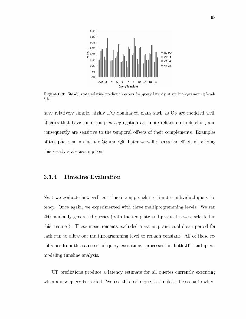
93
!"#
$"#
%!"#
%$"#
&!"#
&$"#
'!"#
'$"#
(!"#
)*+# '# (# $# ,# -# .# %!# %(# %.# %/#
!"#$$%$"
&'($)"*(+,-./("
012#34*#
567#'#
567#(#
567#$#
Figure 6.3: Steady state relative prediction errors for query latency at multiprogramming levels3-5
have relatively simple, highly I/O dominated plans such as Q6 are modeled well.
Queries that have more complex aggregation are more reliant on prefetching and
consequently are sensitive to the temporal offsets of their complements. Examples
of this phenomenon include Q3 and Q5. Later we will discuss the effects of relaxing
this steady state assumption.
6.1.4 Timeline Evaluation
Next we evaluate how well our timeline approaches estimates individual query la-
tency. Once again, we experimented with three multiprogramming levels. We ran
250 randomly generated queries (both the template and predicates were selected in
this manner). These measurements excluded a warmup and cool down period for
each run to allow our multiprogramming level to remain constant. All of these re-
sults are from the same set of query executions, processed for both JIT and queue
modeling timeline analysis.
JIT predictions produce a latency estimate for all queries currently executing
when a new query is started. We use this technique to simulate the scenario where

94
users are submitting queries that are run immediately. This system will enable the
user to estimate how long a new query will take and its projected impact on currently
running queries’ latencies. In this context, we work from the scenario where the user
has no way of predicting the incoming workload. Thus we re-evaluate our latency
predictions every time a new query is introduced into the mix.
This technique also allows us to do real-time “course corrections” for our esti-
mates. We can see how our prediction errors converge as time passes for the JIT
technique in Figure 6.4. Our predictions naturally follow a half-cone shaped dis-
tribution. The closer a query is to completion, the better our predictions are. We
could improve our readings further by evaluating more frequently, perhaps at regular
intervals rather than when we are scheduling a new query. This would be useful if we
are (for example) updating a real-time progress indicator for users who are awaiting
query results or running real-time load balancing.
!"#
$!"#
%!"#
&!"#
'!"#
(!"#
)!"#
!"# %!"# '!"# )!"# *!"# $!!"# $%!"#
!"#$"%&'()"*+',&-'."
!"/('.0,1#2"*((#("
Figure 6.4: JIT prediction errors as we re-evaluate queries periodically at multiprogramming level3.
With the JIT estimator our average error is around 10%. This is a combination of
having good latency estimates paired with corrections from the re-evaluations. This
is the reason that the higher multiprogramming levels generally perform better; they
re-evaluate more frequently as they schedule queries at a faster rate.
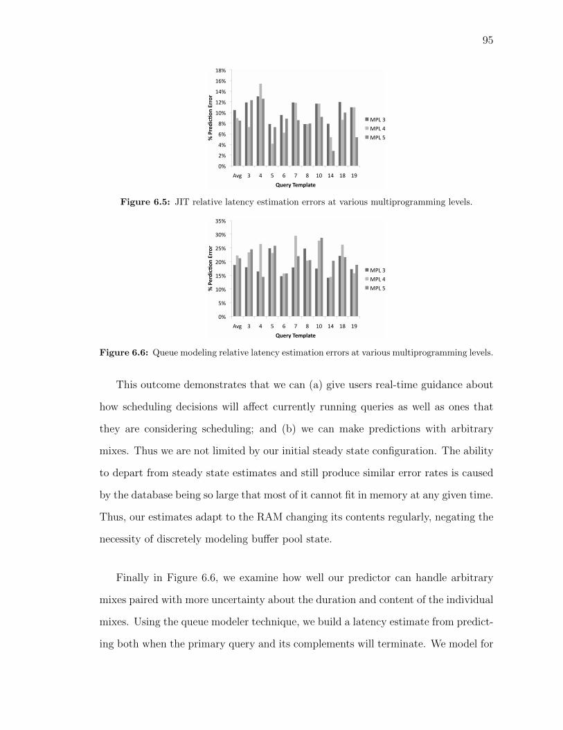
95
!"#
$"#
%"#
&"#
'"#
(!"#
($"#
(%"#
(&"#
('"#
)*+# ,# %# -# &# .# '# (!# (%# ('# (/#
!"#$%&'()*+",$$*$"
-.%$/"0%12345%"
012#,#
012#%#
012#-#
Figure 6.5: JIT relative latency estimation errors at various multiprogramming levels.
!"#
$"#
%!"#
%$"#
&!"#
&$"#
'!"#
'$"#
()*# '# +# $# ,# -# .# %!# %+# %.# %/#
!"#$%&'()*+",%%*%"
-.$%/"0$12345$"
012#'#
012#+#
012#$#
Figure 6.6: Queue modeling relative latency estimation errors at various multiprogramming levels.
This outcome demonstrates that we can (a) give users real-time guidance about
how scheduling decisions will affect currently running queries as well as ones that
they are considering scheduling; and (b) we can make predictions with arbitrary
mixes. Thus we are not limited by our initial steady state configuration. The ability
to depart from steady state estimates and still produce similar error rates is caused
by the database being so large that most of it cannot fit in memory at any given time.
Thus, our estimates adapt to the RAM changing its contents regularly, negating the
necessity of discretely modeling buffer pool state.
Finally in Figure 6.6, we examine how well our predictor can handle arbitrary
mixes paired with more uncertainty about the duration and content of the individual
mixes. Using the queue modeler technique, we build a latency estimate from predict-
ing both when the primary query and its complements will terminate. We model for

96
a continuous multiprogramming level by adding new queries from a provided queue
when complement queries are projected to terminate. The simulation ends when our
primary query is projected to be the next query replaced by an element of the queue.
Overall, this brings our accuracy levels to an average of 21%. This is close to our
estimation accuracy in steady state. This accuracy demonstrates that our framework
can make predictions under realistic scenarios of queries starting and stopping at in-
tervals offset from each other. This allows a user to make straightforward “what-if”
analysis when they are considering scheduling a batch of queries. This framework
could potentially enable a user to formulate different orderings of their queries and
submit them for evaluation to our system. This would search for time-saving order-
ings of submitted queries.
These results also demonstrate that our system can tolerate some uncertainty
about the mixes being executed. Despite our steady state estimates having limited
inherent errors, this does not unduly affect our mixed workload case. In many cases
the timeline errors are not significant because as we are transitioning between mixes,
we do this one query at a time. Thus the subsequent mixes are only slightly different
from each other in terms of how they affect the primary query.
6.2 Contender
Here we evaluate the effectiveness of Contender, our query performance prediction
technique for dynamic workloads.

97
6.2.1 Experimental Configuration
In this work we experimented with TPC-DS [43], a decision support benchmark at
scale factor 100. We executed the benchmark on PostgreSQL 8.4.3. In our deploy-
ment we added the primary key indexes provided by the TPC-DS implementation.
We ran all of our experiments on a machine with an Intel i7 2.8 GHz processors and
8 GB of RAM. The computers had Ubuntu 9.04 on Linux 2.6.28-11 installed.
We elected to work with average running time queries. We sought to target
the workloads that benefit most from our predictions. This is in contrast to long
running queries, which are so demanding that it is often not profitable to run them
concurrently [39]. We omit short running queries because our predictions will benefit
these queries less due to their lifespan.
We identified these queries by first running all of the TPC-DS templates in iso-
lation with a cold cache. We recorded the latency of each template. We sorted the
list by latency and selected the median template and the ones directly below it. Our
workload consisted of 25 templates, 2, 8, 15, 17, 18, 20, 22, 25, 26, 27, 32, 33, 40,
46, 56, 60, 61, 62, 65, 66, 70, 71, 79, 82 and 90. Our workload had a latency range
of 130-1000 seconds in isolation.
We experimented with concurrent mixes at MPLs 2-5 using steady state mixes.
For pairwise interactions (MPL 2) we sampled all pairs. This consisted of 325 distinct
mixes and gave us a comprehensive view of how our queries interacted. We use this
well-sampled dataset to evaluate different components of our model. We did this to
avoid bias in our sampling of this very large space. Naturally for higher MPLs the
number of mixes grows exponentially. At MPL 5 there are 118,755 mixes. Clearly
evaluating this space exhaustively is prohibitively expensive.

98
!"#
$!"#
%!"#
&!"#
'!"#
(!"#
)!"#
*+,# %# -# $(#
$.#
$-#
%!#
%%#
%(#
%)#
%.#
&%#
&&#
'!#
')#
()#
)!#
)$#
)%#
)(#
))#
.!#
.$#
./#
-%#
/!#
!"#$%&"
'#()"%*++,+%
-"./'#0"%
Figure 6.7: Prediction error rate at MPL 4 with CQI-only model.
We used Latin Hypercube Sampling (LHS) to select mixes at higher concurrency
levels as in [3]. Specifically, for all queries in our training set, we randomly selected
mixes such that we have an equal number of samples for each template. We evaluated
four disjoint LHS samples for MPLs 3-5.
Unless otherwise specified we evaluate our models using k-folds cross validation
(k = 5). We partition the data into k equally sized components and repeatedly train
on k − 1 folds, testing on the remaining one.
Our spoiler latency establishes an upper bound for query execution time. How-
ever, there are a small number of cases where the observed latency exceeds the
spoiler’s estimate. This occurred when long running queries are paired with very
short ones and is an artifact of our steady state sampling. When a very short run-
ning query is executed in this manner, its cost of restarting, including generating
the query plan and re-caching dimension tables, becomes a significant part of its re-
source consumption. Empirically we found that overload (latency ≥ 105% of spoiler
maximum) occurs at a frequency of 4%. Identifying these outliers is possible (e.g.,
[4]), however it is beyond the scope of our work. We omit them from our evaluation.

99
6.2.2 Contemporary Query Intensity
In Figure 6.7 we evaluate the effectiveness of using CQI to predict our continuum
point. We build one model per template per MPL based on pairs of CQIs and
continuum points. On average we can predict latency within 18% of the correct
value at MPL 4. This demonstrates a very well-fitted model to these complex query
interactions.
We predict several of our templates very well, within 10% of the correct latency.
These templates are 26, 33, 61 and 71. They are easier to predict because the queries
are extremely I/O bound. All have a pt of 97% or greater, so they are particularly
amenable to CQI modeling.
Templates 2 and 22 had the highest error rates using this technique. Both of
these templates are memory-intensive. They have large intermediate results that
necessitate swapping to disk as contention grows. In Figure 6.8 we look at the CQI
plotted against our observed continuum points for Template 22 at MPL 2. We see
that the pattern of latency growth for this template is closer to logarithmic than
linear, a departure from the behavior of non-memory intensive templates. We did
not have enough similar queries in our workload to train for separate logarithmic
models, so we continue to use the less accurate linear modeling.
Interestingly, template 17, 25, and 32 had slightly lower accuracy. These tem-
plates revolve around random I/O, which makes their response to concurrency less
predictable. Their I/O under concurrency is sensitive to the speed at which we ex-
ecute seeks. Research has found that random I/O can vary by up to an order of
magnitude per page fetched [23].

100
Figure 6.8: Logarithmic trend for memory-intensive Template 22 at MPL 2.
Also we had a slightly higher error rate for Template 40. This template had two
outliers in which it ran with queries that both had high memory and were primarily
random I/O. Without the two outliers, its relative error is reduced to 21%.
6.2.3 Query Sensitivity
In Figure 6.9 we demonstrate that the CQI-only model scales up well in MPLs 2-
5. Our metric is robust to complex and changing concurrent execution conditions.
We found that we could predict new mixes with an error rate of less than 20% on
average.
In this figure we also evaluate our prediction accuracy as we estimate the coeffi-
cients of our query sensitivity models. We start by predicting the model’s slope from
the template’s isolated latency. We then learn the trend line in Figure 4.3 using our
training templates. We apply the estimated slope to learn the y-intercept for each
template. With these parameters, we take in the CQI to produce latency estimates.
We find that we lose around 5% of our accuracy learning y-intercept from a

101
0%
5%
10%
15%
20%
25%
30%
35%
Avg 2 3 4 5
Mean Re
l. Error
Mul-programming Level
CQI Only Y-‐Int Learned QS Learned
Figure 6.9: Mean relative error for predictions with and without knowledge of model parameters.
known slope. This is because we are not perfectly correlated as we make the mapping
between model coefficients. There is some visible noise in the Figure 4.3 and this
creates our slight loss in accuracy.
One important finding in Figure 6.9 is that Contender can create predictions for
multiple previously unseen templates at the same time. When we evaluate learned
QS (and learned slope) our cross validation trains on 20 templates and tests on the
remaining 5. We are simulating the case where 5 new templates are added to our
workload (and we evaluate their interactions with other new templates based only
on their QEPs and isolated pt values). This works for two reasons. First, CQI
is dependent primarily on semantic information, so we do not need to sample our
interactions. Secondly the space demonstrated in Figure 4.3 is simple to model and
requires limited sampling.
Our accuracy in this work is comparable the prior work on cQPP [23]. They were
able to predict query latency within 25% of the correct figure on average on TPC-H
while requiring latin hypercube sampling with each new template. We achieved the
approximately same accuracy using linear time samplings and do not require any
sampling of concurrent mixes.

102
6.2.4 Spoiler Estimation
Next we turn our attention to predicting spoiler latency for individual templates.
In Figure 6.10 we evaluate our accuracy for predicting MPLs 2-5. In the perfect
linear series we evaluate how predictable spoiler latency is for direct models, where
we build directly on sampled points to see how much noise is inherent in the system.
After that we evaluate our sampled approach in which we predict spoiler latency at
MPLs 4-5 based on sampling MPLs 1-3. Next we compared our two comprehensive
predictors of spoiler growth, k nearest neighbors and pt regression. For this section
we train on all but the test template and evaluate our model on the remaining one.
In the perfect linear case we fit a trend line to our spoiler latency at the five
sampled levels and take the mean relative error of our observed latencies as they
deviate from the trend line. Our predictions were within 5% of the correct latency
on average. For most queries our growth is directly proportional to the simulated
MPL. We verify our initial conjecture that fair sharing will stretch out our latency
in a linear fashion.
Next we evaluated spoiler latency predictions with reduced sampling. We learned
from MPLs 1-3 and predicted the remaining two multiprogramming levels. This
limited sampling established a trajectory for our spoiler latency. We found that
on average we could predict spoiler latency within slightly better than 10% of the
correct figure using this technique.
Next we predicted spoiler latencies using the KNN approach. We found the k
templates nearest to our test template (k = 3) and averaged their models to predict
the spoiler latencies of the new template. We evaluated the k nearest templates in a
2-D space where we considered a template’s pt and working set size. This approach

103
!"#
$"#
%!"#
%$"#
&!"#
&$"#
&# '# (# $#
!"#$%&"
'(%)**+*%
!,'-.*+/*#001$/%2"3"'%
)*+,*-.#/01*2+#
32456*7#
899#
5.#
Figure 6.10: Spoiler estimation error rate with several prediction strategies. Relative error dis-played.
allows us to create predictions for completely new templates without sampling their
spoiler performance. However it brought our accuracy down for a MRE of 15%.
Finally, we created predictions based on linear regression, relating pt of the new
template to training model coefficients. This approach allowed us to solve for the
coefficients on a continuous function rather than working from a nearest neighbor fit.
However it incorporated less information by only working with our most correlated
variable, pt. It performed slightly worse than KNN with a MRE of 20%.
We then used our estimated spoiler times to create concurrent query latency
predictions. As with the prior experiments, we first create continuums establishing
the estimated spoiler latency as our upper bound. In Figure 6.11 we average over all
of our templates except for Template 2.
Template 2 has a very large working set size. This causes the spoiler to grow at
a much faster rate than than is common in our workload, especially at higher MPLs.
This behavior is the result of the spoiler always exceeding its portion of the RAM,
forcing the query to swap. It dramatically increases our upper bound. In practice this
template is getting better resource access than the spoiler-predicted maximum due to

104
!"#
$!"#
%!"#
&!"#
'!"#
(!!"#
($!"#
$# )# %# *#
!"#$%&"
'(%)**+*%
!,'-.*+/*#001$/%2"3"'%
+,-.,#/0-1234#
+55#/0-1234#
6722#89:;#
Figure 6.11: Latency predictions with estimated spoiler and isolated I/O profile. Error bars arestandard deviations.
sharing work with the contemporaries. Hence our estimated spoilers, which are lower
than the actual spoiler latency in this case, produce artificially better predictions by
limiting the prediction range. This is because there were few potential neighbors
that had comparable working sets. In future work we can mitigate this effect by
creating a suite of spoilers, each consuming different quantities of RAM.
We found that working from these estimated spoiler latencies did not significantly
affect the accuracy of our predictions. In most cases the spoiler latency estimates
were sufficiently close such that it did not impact our ability to predict template
latency in individual mixes. However, as the figure demonstrates, the standard
deviation of our predictions increase. There is more noisiness in our data as we
learn spoiler growth patterns from the k-nearest neighbors. We demonstrate that by
sampling a query only in isolation we can build a profile to predict its latency with
a mean relative error of 25%.
Finally we experimented with predicting query performance under concurrency
simulating the case of using the inputs from a QPP model for queries executing in
isolation such as [9]. The final series in Figure 6.11 demonstrates our prediction
accuracy when we randomly assign our prediction inputs as ± 25% of their observed
values. This error rate is in line with the isolated prediction accuracy in the literature.

105
!"# !$# !%# !"# !$# !%#
!%# !"# !$# !%# !"# !$# !%#
!$# !%# !"# !$# !%# !"#
&'#
&(#
&)#
*+,-#
Figure 6.12: Example workload for throughput evaluation with three streams with a workload ofa, b, and c.
We found a commensurate loss in accuracy in our predictions.
6.3 Portable Predictions
In this section, we first detail our experimental configurations. We then explore the
cloud response surface, for which we are building our models. Next, we evaluate the
effectiveness of our prediction framework for cloud performance based on complete
sampling of the local response grid. After that, we investigate how our system
performs with our two sampling strategies. Finally, we look at the efficacy of our
models gaining feedback from cloud sampling.
6.3.1 Experimental Configuration
We experimented with TPC-DS and TPC-H, two popular analytical benchmarks at
scale factor 10. We evaluated using all but the 5 longest running queries on TPC-
H and using 74 of the 100 TPC-DS templates, again omitting the longest running
ones. We did not use the TPC-DS templates that ran for greater than 5 minutes in
isolation on our highest local hardware configuration. We elected to omit the longest
running queries because under concurrency their execution times grow very rapidly
and we kept the scope of our experiments to 24 hours or less each. Nonetheless

106
a portion of our experiments (2%) still exhibited unbounded latency growth. We
terminated them after 24 hours and record them as having zero QpM.
We implemented a variant of the TPC-H throughput test. An example of our
setup is displayed in Figure 6.12. Specifically we created a workload with 5 templates,
± 1 to account for modulus cases. Our trials were all at multiprogramming level 3,
in accordance with TPC-H standards. Each of our three query streams executed a
permutation of the workload’s templates. We executed at least 5 examples of each
stream before we concluded our test. We omit the first and last few queries from
each experiment to account for a warmup and cool down time. We compute the
queries per minute (QpM) for the duration of the experiment.
We created 23 TPC-DS workloads using this method. The first 8 were configured
to look at increasing database sizes. The first two access tables totaling to 5 GB,
the second two at 10 GB, et cetera. The remaining 15 workloads were randomly
generated without replacement. For TPC-H we randomly generated 9 workloads.
There were three sets of three permutations without replacement.
We quantify the quality of our predictions using mean relative error as in [23,
9, 5]. We compute it for each prediction as |observed−predicted|observed
. This metric scales our
predictions by the throughputs, giving an intuitive yardstick for our errors.
For our in-cloud evaluations we used Amazon EC2 and Rackspace. We rented
EC2’s m1.medium, m1.large, m1.xlarge and hi1.4xlarge instances. The first three are
general purpose virtual machines at increasing scale of hardware. The final is an I/O
intensive SSD offering. We considered experimenting on their micro instances and
conducted some experiments on AWS’s m1.small offering. However we found that so
many of our workloads do not complete within our time requirement in this limited

107
setting that we ceased pursuing this option. When a workload greatly outstrips the
hardware resources available it is reduced to thrashing as it swaps continuously. In
Rackspace we experimented on their 4, 8, 16, and 32 GB cloud offerings.
We used k-fold cross validation (k=4) for all of our trials. That is, we partition
our workloads into k equally sized folds, train on k−1 folds and test on the remaining
one.
6.3.2 In Cloud Performance
In Figure 6.13 we detail the throughput for our individual workloads as they are
deployed on a variety of cloud instances. We see a monotonic surface much like the
ones that we encounter with the local testbed. This indicates that there may be
exploitable correlations between the two surfaces.
For TPC-H we see that the majority of our workloads are of moderate intensity.
They have a gradual increase in performance until they reach the extra large instance.
At that point many of the workloads fit in the 7.5 GB of memory, seeing only modest
gains from the largest instance. There are three workloads that are more intensive
(shown in dashed lines). They have greater hardware requirements and do not see
performance gains until the database is completely memory resident.
TPC-DS has a more diverse response to the cloud offerings. The majority follow
a curve similar to that of TPC-H. There is one that never achieves performance
gains because it is entirely CPU bound. We also have two examples of the memory-
intensive “knee” as seen in TPC-H, again as a dashed line. The consistency of the
response surfaces also indicates that our cloud evaluation was robust to noisiness

108
!"
#"
$"
%"
&"
'"
("
)"
*"
+"
,-./01" 2345-" 67345-" 8/59":;<"!"#$%#&'(')%*"+#'
,-.'/*&+0*1#'
!"
$"
&"
("
*"
#!"
#$"
#&"
#("
#*"
,-./01" 2345-" 67345-" 8/59":;<"
!"#$%#&'(')%*"+#'
,-.'/*&+0*1#'
=3>" =?>"
Figure 6.13: Cloud response surface for (a) TPC-H and (b) TPC-DS
that is a part of the multi-tenant cloud environment.
Next we examine the quality of our predictions for a new workload if we have
very good knowledge of its local response surface. For each workload we sampled
the entire grid in Figure 5.3 locally. Our prediction results are in Figure 6.14. We
observed that the quality of our predictions steadily increased for TPC-DS with our
provisioned hardware. As the workloads had more resources they thrash and swap
less. This makes their outcomes more predictable.
In contrast our predictions in TPC-H get slightly worse for the larger instances.
This is a side effect of the three dashed workloads that are memory-intensive. They
exhibit limited growth in the smaller instances and have a dramatic take off when
they have sufficient RAM. This is an under-sampled condition. If we omit them from
our calculations, our average error drops to 20% for the highest two instances.
It is interesting to see that these two response surfaces in Figure 6.13 are very
comparable despite their different schemas. This demonstrates that both analytical
benchmarks are highly I/O bound and that we have fertile ground to learn across
databases rather than having to deploy a new database in the cloud before we can

109
!"#
$"#
%!"#
%$"#
&!"#
&$"#
'!"#
'$"#
(!"#
)*+# ,-./01# 234+-# 5634+-# 7/+8#9:;#
!"#$%&"
'#()"%*++,+%
-./%0$12#$3"%
<=>?@A#
<=>?7#
Figure 6.14: Prediction errors for cloud offerings.
make predictions.
6.3.3 Cross Schema Prediction
We found that we could predict TPC-DS based on TPC-H only training within 27%
of the correct throughput on average. The results showed encouraging evidence that
the framework can successfully identify the important similarities across workloads
that are drawn from different set of queries and schemas.
6.3.4 Sampling
Next we quantify the speed at which adaptive sampling converged on a response
surface. We configured our algorithm such that if the range is less than 1 QpM
we cease sampling. We made our stopping condition for recursion 33% of the range
established by the initial, most distant points. We found that on average we sampled
43% of the space for TPC-DS and 33% for TPC-H.
This is a very high sampling rate, considering that our local trials take 165
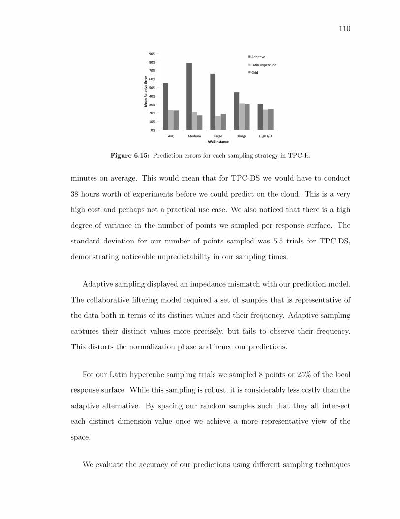
110
!"#
$!"#
%!"#
&!"#
'!"#
(!"#
)!"#
*!"#
+!"#
,!"#
-./# 012345# 678/1# 9:78/1# ;3/<#=>?#
!"#$%&"
'#()"%*++,+%
-./%0$12#$3"%
67AB#;C@18D4E1#
F832#
Figure 6.15: Prediction errors for each sampling strategy in TPC-H.
minutes on average. This would mean that for TPC-DS we would have to conduct
38 hours worth of experiments before we could predict on the cloud. This is a very
high cost and perhaps not a practical use case. We also noticed that there is a high
degree of variance in the number of points we sampled per response surface. The
standard deviation for our number of points sampled was 5.5 trials for TPC-DS,
demonstrating noticeable unpredictability in our sampling times.
Adaptive sampling displayed an impedance mismatch with our prediction model.
The collaborative filtering model required a set of samples that is representative of
the data both in terms of its distinct values and their frequency. Adaptive sampling
captures their distinct values more precisely, but fails to observe their frequency.
This distorts the normalization phase and hence our predictions.
For our Latin hypercube sampling trials we sampled 8 points or 25% of the local
response surface. While this sampling is robust, it is considerably less costly than the
adaptive alternative. By spacing our random samples such that they all intersect
each distinct dimension value once we achieve a more representative view of the
space.
We evaluate the accuracy of our predictions using different sampling techniques

111
in Figure 6.15. We see that adaptive sampling does very poorly in comparison to the
full grid and Latin hypercube approaches. This is because we oversample the spaces
that exhibit rapid change and do not give due weight to the ones that are more stable
and likely to be the average case. In future work we could mitigate this limitation by
interpolating the response surface based on known points. Latin hypercube sampling
demonstrates prediction accuracy on par with that of grid sampling, showing that
this approach is well-matched to our prediction engine. We do perform slightly better
in the m1.large case. This is a 2% difference is a negligible noise due to the spoiler
simulations.
In Figure 6.16 we compare (1) our TPC-DS predictions on Rackspace with
Latin hypercube sampling to (2) those that are based on LHS and incorporating
m1.medium and m1.xlarge samples from our AWS experiments. For the LHS-only
sampling case we found that it was slightly harder to predict than in Amazon AWS.
The response surfaces on Rackspace were slightly less smooth than AWS, implying
that multi-tenancy may have been playing a larger role in this environment.
In the second series (shown as Local LHS+AWS), we evaluated how augmenting
our models with cloud samples would improve our predictions. We found that this
feedback modestly but appreciably increased our accuracy. This demonstrated that
our incremental improvement of the model benefits from the feedback and that cross-
cloud knowledge is portable.

112
!"#
$!"#
%!"#
&!"#
'!"#
(!"#
)!"#
*+,# -.',/# -.0,/# -.$),/# -.&%,/#
!"#$%&"
'#()"%*++,+%
&#-./0#-"%1$/2#$-"%
12345#167#
12345#167#8#*97#
Figure 6.16: Prediction accuracy for TPC-DS on Rackspace based on Latin hypercube sampling,with and without additional cloud features.

Chapter Seven
Related Work

114
Extensive work has been done in the area of characterizing queries and their per-
formance. This includes analytical estimates such as those used by query optimiz-
ers [49], black-box profiling [3] and hybrid approaches [26]. Query performance pre-
diction has also been considered for many workload types including OLAP [3] and
MapReduce [41]. The problems solved by these works includes query scheduling,
latency prediction and many other problems. There has been some work done on
analytically predicting throughput in [25]. In this section we examine the state of
the art for our proposed work.
The importance of query performance prediction is explored in [10]. Query per-
formance prediction can allow us to enhance almost all aspects of a database from
its physical design to query execution planning. In other words, predictive databases
can create an introspective system that is self-tuning and self-scheduling.
7.1 Query interaction modeling
The topic of performance predictions for database workloads has gained significant
interest in the research community. In [26] the authors use machine learning tech-
niques to predict the performance metrics of database OLAP queries. Although their
performance metrics include our QoS metric (query latency), their system does not
address concurrent workloads. Moreover, their solution relies on statistics from the
SQL text of a query or obtained from the optimizer on the query plan. Prior efforts to
predict database performance [36, 58] provide an estimate of the percentage of work
done or produce an abstract number intended to represent relative “cost”. In [13]
the authors analyzed how to classify workloads. Work has been done to characterize
the usage of specific resources in databases including [12] and [34] examine memory

115
and CPU usage under various workloads respectively.
In [37] the researchers propose a single query progress indicator that can be
applied on a large subset of database query types. Their solution uses semantic
segmentation of the query plans and strongly relies on the optimizer’s (often inac-
curate) estimates for cardinality and result sizes. Although their progress estimator
takes into account the system load, their work does not specifically estimate progress
of concurrent queries and includes limited experiments on resource contention. On
the contrary, our work primarily focuses on concurrent workloads and does not rely
on the optimizer’s estimates. Moreover, our timeline analysis identifies the overlap
between concurrent queries to continuously improve the prediction error and thus
can effectively address resource contention for concurrent queries. Finally, progress
estimators have been investigated for MapReduce queries [41]. Although this work
is related, it assumes a different workload model from the one used in this paper.
Furthermore, [38] examines predicting query latency with concurrency, but does not
consider multiple, diverse query classes.
Query interactions have also been addressed and greatly advanced in [2, 3] and [4].
In this work the authors create these concurrency-aware models to build schedules
for batches of OLAP queries. Their solutions create regression models based on
sampling techniques similar to the ones that we use. These systems created schedules
for a list of OLAP queries to minimize end-to-end latency for a large set of queries.
Our experiment-driven approach predicts the response time of individual queries,
and presumes that the order of execution of the queries is fixed for a real-time
environment.
[7] models the mixes of concurrent queries over time from a provided workload,
but does not target individual query latencies, instead optimizing for end-to-end
116
workload latencies. This approach uses an incremental evaluation approach, which
our timeline analysis is inspired by. Our timeline modeling uses a very different
framework to project latency.
In [29] the authors use machine learning to predict query performance. They
provide a range for their query execution latency. Their work considers concurrency
as well, but only looks at the multiprogramming level rather than individual mixes.
In contrast, we provide a scalar estimate and consider system strain at a higher
granularity.
Finally, [39] explores how to schedule OLAP mixes by varying the multiprogram-
ming level. They use a priority-based control mechanism to prevent overload and
underload, allowing the database to maintain a good throughput rate. Like this
work, our model experiments for many multiprogramming levels, but our focus in
this work is in predicting QoS rather than scheduling the right degree of concurrency.
7.2 Qualitative Workload Modeling
Qualitative workload modeling is used to compare competing options when planning
how to schedule or manage a workload. There has been considerable work on this
for cloud deployment [54, 46, 32, 60]. It has also been considered in the context of
power management [56, 15]. Similar modeling has been explored for for transactional
workloads in [28, 19, 47].
117
7.3 Query Resource Profiling
In [46] we created generic bin packer for the provisioning of cloud resources. For this
study our objectives revolved around solving for minimum financial cost in creat-
ing virtual machine deployment plans on the cloud. Our generic query performance
prediction is a logical extension of this work, but instead optimizes for query perfor-
mance goals. Whereas the prior work considered black- and white-box approaches,
we propose gray box performance prediction. We strive to leverage the best elements
of both approaches.
Our BAL framework is an inversion of the techniques for configuration of virtual
machines in [51] and automatic deployment of virtualized applications [50]. In [51]
the researchers exploit database cost models to determine the appropriate resource
configuration for the virtual machines on which an anticipated workload will run.
In their model, resource allocation can be applied in a more fine-grained manner
by provision specific amounts of memory, CPU power, I/O bandwidth, etc. In our
approach, the system begins with pre-configured physical machines. In [50] virtu-
alized applications are treated as black-boxes and performance modeling techniques
are used to predict the performance of these applications on different machines con-
figurations. In contrast, our approach is specific to database systems and it attempts
to exploit database cost models to achieve its objectives.
Resource management and scheduling have also been addressed within the con-
text of database systems [26, 42]. In [20, 27, 40] they allocate a fixed pool of resources
to individual queries or query plan operators and scheduling queries or operators to
be executed on the available resources aiming to increase the system throughput.
We extend this work by focusing on analytical query-oriented workloads rather than
118
throughput-based goals.
Resource provisioning for shared computers has been studied extensively in the
operating system community. In [52] the authors use a profiling approach to over-
booking resources with a graph-based placement algorithm. Their work focuses on
supporting many heterogeneous applications in a cluster where each unit of applica-
tion can only exist on one node. Ours starts with a similar problem and progresses
on to the inverse, dividing a database application among multiple nodes.
In [21] the authors study a similar resource provisioning problem for web-based
applications using a modeling approach. Their work also naturally lends itself to
bin-packing, but it is tailored for web server applications only, focusing more on
cache locality and modeling how the workload evolves over time. They also do not
use profiling and presume a finer-grained degree of control (being able to allocate
memory on a per-application basis) than is possible with a large-scale database
deployment.
Workload characterization for three-tiered web services was examined in [57]. The
authors use neural networks to distill the relationship between system configuration
and workload performance. They primarily focused on predicting efficient system
configurations whereas our work is concerned with making scheduling decisions on a
fixed configuration.
In [59] the authors characterize generic database workloads to create represen-
tative benchmarks. They examine system traces and SQL statements to classify a
workload. Their work characterizes the resources used by individual queries. In con-
trast our research takes a known workload, analyzes its resource consumption and
makes performance predictions.

119
7.4 Query Progress Indicators
There has been robust work on query progress indicators [16, 17, 37, 38] and existing
solutions are covered in [16]. In [17] the authors reason about the percent of the query
completed, however their solution does not directly address latency predictions for
database queries and they do not consider concurrent workloads. [38, 37] do consider
system strain and concurrency, but they remain focused on performance of queries
in progress. In contrast, we create predictions for queries before they begin.
7.5 Query Performance Prediction
In [9, 26] the researchers use machine learning techniques to predict multiple per-
formance metrics of analytical queries. Although their predictions include our QoS
metric (query latency), they do not address the problem of concurrent workloads. In
Section 4.1 we experimented with the same machine learning techniques and found
them unsuitable for cQPP. Furthermore, in [9] the researchers propose predictive
modeling techniques and they use two types of prediction models, namely support
vector machines (SVMs) and Kernel Canonical Correlation Analysis (KCCA). This
work studies query latency prediction models for both static and dynamic workloads.
In addition [35] examined statistical techniques to further generalize prediction for
isolated query performance prediction.
Performance prediction under concurrency was pioneered and well-modeled in [3,
4]. The authors create concurrency-aware models to build schedules for batches of
OLAP queries. Their solutions create regression models based on sampled concurrent
query executions. These systems generate optimal schedules for a set of OLAP
120
queries to minimize end-to-end latency for an entire batch. Our experiment-driven
approach provides finer grained predictions that can estimate the response time of
individual queries. Furthermore, [7, 8] extends the work in [3, 4] to predict the
completion time of mixes of concurrent queries over time from a provided workload.
This work does not target individual query latencies either; instead the authors
predicted end-to-end workload latencies. Similar to this work, we learn from well-
defined templates. However, we do not require sampling how these templates interact
with the workload to make predictions.
[29, 39] explored workload modeling under concurrency. [29] makes predictions
about query latency under concurrency as a range. Neither of these approaches make
precise latency predictions as we do in this work. In [39] the authors consider query
interactions to tune the multiprogramming level and guide query scheduling.
Finally in [23] we proposed predictive performance models for concurrent work-
loads. This research showed that a new buffer access latency metric can be highly
effective in capturing resource contention across concurrent workloads. However the
techniques proposed were limited to predictions for known templates with sampling
requirements exponential in the number of query templates to be supported. The
proposals in this paper address these limitations without sacrificing predictive accu-
racy.
Workload Characterization
In [24] the authors created a system to automatically classify workloads as ana-
lytical or transactional. In [48] the researchers explored different types of transac-
tional workloads and how the implementation of an OLTP workload can dramatically
impact its performance characteristics. [5] examined how to identify individual an-

121
alytical templates within a workload. In [30] researchers analyzed how individual
components of traditional RDBMSs contribute to latency. All of these techniques
can help us create generalized models for database workloads.
There has also been work on profiling and managing workload performance in
the cloud. In [53, 55, 61] the authors managed workloads from the perspective of
maximizing profits from service level agreements (SLAs). In [18, 19] the researchers
built models to profile workloads for multi-tenant databases in the cloud. Database
consolidation was studied in [6]. Analytical query interactions were modeled in [3, 4].
In [22], the researchers presented a system for automatically managing database pa-
rameters for a workload. Our approach is similar to this work in that we characterize
a multidimensional response surface for workloads under varying conditions.
To the best of our knowledge, no prior work addressed the problem of predicting
workload performance for changing hardware platforms.

Chapter Eight
Conclusion

123
In this section we highlight the main findings of our studies. We will examine our pre-
diction framework for static and dynamic workloads as well as portable predictions.
Finally we will identify several future research directions in this area.
8.1 Concurrent Query Performance Prediction for
Static Workloads
This work proposes a lightweight estimator for concurrent query execution perfor-
mance for analytical workloads. To the best of our knowledge it is the first to
predict execution latency for individual queries for real-time reporting without using
semantic information.
Our system starts with studying the relationship between BAL and quality of
service as measured by query execution latency. We have demonstrated that there
is a strong linear relationship between these two metrics, which we model with our
system B2L. This relationship is based on the observation that as long as there is
contention for a resource and we can instrument its bottleneck, then we can ac-
curately predict latency. We produce very accurate estimates of latency given the
average BAL despite this metric exhibiting moderate variance. We accomplish this
because our queries are sufficiently long that we collect enough samples to produce
a representative average. This naturally is proportional to the latency because the
queries are primarily I/O-bound. We predict the BAL by extrapolating higher degree
interactions using pairwise BALs in a system we call B2cB.
We then adapt this baseline system to a dynamically changing workload using
timeline analysis. We predict the steady state latency of each query in a workload

124
and determine which will terminate first. We then estimate the progress of each query
after the first terminates and conjecture about which will end next. We continue
this cycle in two formulations: just-in-time and queue-modeler. In the former, we
build our prediction based on the currently executing batch. The latter fixes our
multiprogramming level and predicts when new queries will be started as old ones
end.
8.2 Concurrent Query Performance Prediction for
Dynamic Workloads
We studied the problem of predicting concurrent performance of dynamic analytical
query workloads. This is a problem with many important applications in resource
scheduling, provisioning, and user experience management. This tool may also be
useful for next generation query optimizers by modeling and predicting contention
within the I/O subsystem.
We first showed that existing machine learning approaches for query performance
prediction do not provide satisfactory solutions when extended for concurrency. We
then described our solution, which we call Contender. It relies on modeling the
degree to which queries create and are affected by resource contention. We formally
defined and quantified these notions via two new metrics called Contemporary Query
Intensity (CQI) and Query Sensitivity (QS), respectively. Using these metrics and
the knowledge of baseline (i.e., isolated) query performance, we were able to make
accurate predictions for arbitrary queries with low training overhead.
Specifically, our experiments using PostgreSQL on TPC-DS showed our predic-
125
tion errors can be kept within 25% with constant time sampling overhead. Our
approach is thus competitive with alternative techniques in terms of predictive ac-
curacy, yet it constitutes a substantial improvement over the state of the art, as
it is both more general (i.e., supports predictions on arbitrary queries), and more
practical and efficient (i.e., require less training).
8.3 Workload Performance Prediction for Portable
Databases
In this work we introduce the problem of creating performance predictions for portable
databases with analytical workloads. Our framework creates workload fingerprints
by simulating various hardware configurations. We train our collaborative learning
models using these signatures. This approach allows us to predict throughput as the
databases migrates to different cloud offerings. Our prediction framework enables
users to “right size” their provisioning and cloud deployments.
We first discuss how we created a local testbed and simulate different hardware
configurations to profile our workload. After that we explored how we brought
collaborative filtering to bear on this problem. Finally we explore two sampling
approaches to reduce our training time: adaptive sampling and Latin hypercube.
We have demonstrated that using these techniques we can predict workload
throughput, on TPC-H and TPC-DS, within approximately 30% of the correct value
on average. These results are obtained by sampling only a quarter of the local
response surface, which makes our solution practical for low-overhead deployment.
126
One interesting extension to this problem could be predicting the latency of
individual queries as they are moved from one hardware platform to another. This
could be studied either in isolation or under concurrency. In either context it would
make portable databases more accessible to users.
Future research in this area could also include generalizing our models to accom-
modate growing and shrinking databases. By scaling our predictions, we may be
able to support incrementally changing workloads. This would further improve the
usability and applicability of our approach.
Another research direction in this area is modeling transactional workloads under
changing hardware configurations. The underpinnings of this model would be differ-
ent because it would need to take into account latches, locks and other more complex
interactions among write-intensive queries. It too would make portable databases
more accessible to users. This more detailed modeling is beyond the scope of this
work.
In summary we created a system to fingerprint analytical workloads by using
a locally executed testbed to simulate a variety of hardware platforms. We then
compare this profile to that of other analytical workloads using collaborative filtering.
We use careful sampling to further reduce our training time and cost.

Bibliography
[1] Ashraf Aboulnaga, Kenneth Salem, Ahmed A. Soror, Umar Farooq Minhas,Peter Kokosielis, and Sunil Kamath. Deploying database appliances in thecloud. IEEE Data Eng. Bull., 32(1):13–20, 2009.
[2] Mumtaz Ahmad, Ashraf Aboulnaga, and Shivnath Babu. Query interactions indatabase workloads. In DBTest, 2009.
[3] Mumtaz Ahmad, Ashraf Aboulnaga, Shivnath Babu, and Kamesh Munagala.Modeling and exploiting query interactions in database systems. In CIKM ’08:Proceeding of the 17th ACM conference on Information and knowledge manage-ment, pages 183–192, New York, NY, USA, 2008. ACM.
[4] Mumtaz Ahmad, Ashraf Aboulnaga, Shivnath Babu, and Kamesh Munagala.Qshuffler: Getting the query mix right. In ICDE ’08: Proceedings of the 2008IEEE 24th International Conference on Data Engineering, pages 1415–1417,Washington, DC, USA, 2008. IEEE Computer Society.
[5] Mumtaz Ahmad, Ashraf Aboulnaga, Shivnath Babu, and Kamesh Muna-gala. Interaction-aware scheduling of report-generation workloads. VLDB J.,20(4):589–615, 2011.
[6] Mumtaz Ahmad and Ivan T. Bowman. Predicting system performance for multi-tenant database workloads. In DBTest, page 6, 2011.
[7] Mumtaz Ahmad, Songyun Duan, Ashraf Aboulnaga, and Shivnath Babu.Interaction-aware prediction of business intelligence workload completion times.In ICDE, pages 413–416, 2010.
[8] Mumtaz Ahmad, Songyun Duan, Ashraf Aboulnaga, and Shivnath Babu. Pre-dicting completion times of batch query workloads using interaction-aware mod-els and simulation. In EDBT, pages 449–460, 2011.
[9] Mert Akdere, Ugur Cetintemel, Matteo Riondato, Eli Upfal, and Stanley B.Zdonik. Learning-based query performance modeling and prediction. In ICDE,pages 390–401, 2012.
127

128
[10] Mert Akdere, Ugur Cetintemel, Matteo Riondato, Eli Upfal, and Stanley B.Zdonik. The case for predictive database systems: Opportunities and challenges.In CIDR, 2011.
[11] Amazon. Amazon web services. http://aws.amazon.com/.
[12] Luiz Andre Barroso, Kourosh Gharachorloo, and Edouard Bugnion. Memorysystem characterization of commercial workloads. In ISCA ’98: Proceedings ofthe 25th annual international symposium on Computer architecture, pages 3–14,Washington, DC, USA, 1998. IEEE Computer Society.
[13] Maria Calzarossa and Giuseppe Serazzi. Workload characterization: A survey.In Proceedings of the IEEE, pages 1136–1150, 1993.
[14] Chih-Chung Chang and Chih-Jen Lin. LIBSVM: A library for support vectormachines. ACM Transactions on Intelligent Systems and Technology, 2:27:1–27:27, 2011.
[15] Jeffrey S. Chase, Darrell C. Anderson, Prachi N. Thakar, Amin M. Vahdat,and Ronald P. Doyle. Managing energy and server resources in hosting centers.SIGOPS Oper. Syst. Rev., 35(5):103–116, October 2001.
[16] Surajit Chaudhuri, Raghav Kaushik, and Ravishankar Ramamurthy. When canwe trust progress estimators for sql queries? In SIGMOD ’05: Proceedingsof the 2005 ACM SIGMOD international conference on Management of data,pages 575–586, New York, NY, USA, 2005. ACM.
[17] Surajit Chaudhuri, Vivek Narasayya, and Ravishankar Ramamurthy. Estimat-ing progress of execution for sql queries. In SIGMOD ’04: Proceedings of the2004 ACM SIGMOD international conference on Management of data, pages803–814, New York, NY, USA, 2004. ACM.
[18] Carlo Curino, Evan Jones, Raluca Ada Popa, Nirmesh Malviya, Eugene Wu,Samuel Madden, Hari Balakrishnan, and Nickolai Zeldovich. Relational Cloud:A Database Service for the Cloud. In 5th Biennial Conference on InnovativeData Systems Research, Asilomar, CA, January 2011.
[19] Carlo Curino, Evan P.C. Jones, Samuel Madden, and Hari Balakrishnan.Workload-aware database monitoring and consolidation. In Proceedings of the2011 ACM SIGMOD International Conference on Management of data, SIG-MOD ’11, pages 313–324, New York, NY, USA, 2011. ACM.
[20] Diane Davison and Goetz Graefe. Dynamic Resource Brokering for Multi-UserQuery Execution. 1995.
[21] Ronald P. Doyle, Jeffrey S. Chase, Omer M. Asad, Wei Jin, and Amin M. Vah-dat. Model-based resource provisioning in a web service utility. In USITS’03:Proceedings of the 4th conference on USENIX Symposium on Internet Technolo-gies and Systems, pages 5–5, Berkeley, CA, USA, 2003. USENIX Association.
[22] Songyun Duan, Vamsidhar Thummala, and Shivnath Babu. Tuning databaseconfiguration parameters with ituned. PVLDB, 2(1):1246–1257, 2009.
129
[23] Jennie Duggan, Ugur Cetintemel, Olga Papaemmanouil, and Eli Upfal. Perfor-mance prediction for concurrent database workloads. In SIGMOD Conference,pages 337–348, 2011.
[24] Said Elnaffar, Patrick Martin, Berni Schiefer, and Sam Lightstone. Is it dssor oltp: automatically identifying dbms workloads. volume 30, pages 249–271,2008.
[25] Sameh Elnikety, Steven Dropsho, Emmanuel Cecchet, and Willy Zwaenepoel.Predicting replicated database scalability from standalone database profiling. InProceedings of the 4th ACM European conference on Computer systems, EuroSys’09, pages 303–316, New York, NY, USA, 2009. ACM.
[26] Archana Ganapathi, Harumi Kuno, Umeshwar Dayal, Janet L. Wiener, Ar-mando Fox, Michael Jordan, and David Patterson. Predicting multiple metricsfor queries: Better decisions enabled by machine learning. In ICDE ’09: Pro-ceedings of the 2009 IEEE International Conference on Data Engineering, pages592–603, Washington, DC, USA, 2009. IEEE Computer Society.
[27] Minos N. Garofalakis and Yannis E. Ioannidis. Multi-dimensional resourcescheduling for parallel queries. In Proceedings of the 1996 ACM SIGMOD in-ternational conference on Management of data, SIGMOD ’96, pages 365–376,New York, NY, USA, 1996. ACM.
[28] Rachid Guerraoui, Maurice Herlihy, and Bastian Pochon. Toward a theory oftransactional contention managers. In Proceedings of the twenty-fourth annualACM symposium on Principles of distributed computing, PODC ’05, pages 258–264, New York, NY, USA, 2005. ACM.
[29] C. Gupta, A. Mehta, and U. Dayal. Pqr: Predicting query execution timesfor autonomous workload management. In Autonomic Computing, 2008. ICAC’08. International Conference on, pages 13 –22, 2008.
[30] Stavros Harizopoulos, Daniel J. Abadi, Samuel Madden, and Michael Stone-braker. Oltp through the looking glass, and what we found there. In Proceedingsof the 2008 ACM SIGMOD international conference on Management of data,SIGMOD ’08, pages 981–992, New York, NY, USA, 2008. ACM.
[31] Dietmar Jannach, Markus Zanker, Alexander Felfernig, and Gerhard Friedrich.Recommender Systems: An Introduction. Cambridge University Press, 2010.
[32] Verena Kantere, Debabrata Dash, Georgios Gratsias, and Anastasia Ailamaki.Predicting cost amortization for query services. In SIGMOD Conference, pages325–336, 2011.
[33] Alexandros Karatzoglou, Alex Smola, Kurt Hornik, and Achim Zeileis. kernlab –an S4 package for kernel methods in R. Journal of Statistical Software, 11(9):1–20, 2004.
[34] Kimberly Keeton, David A. Patterson, Yong Qiang He, Roger C. DSRaphael,and Walter E. Baker. Performance characterization of a quad pentium pro

130
smp using oltp workloads. In ISCA ’98: Proceedings of the 25th annual inter-national symposium on Computer architecture, pages 15–26, Washington, DC,USA, 1998. IEEE Computer Society.
[35] Jiexing Li, Arnd Christian Konig, Vivek R. Narasayya, and Surajit Chaud-huri. Robust estimation of resource consumption for sql queries using statisticaltechniques. PVLDB, 5(11):1555–1566, 2012.
[36] Jack L. Lo, Luiz Andre Barroso, Susan J. Eggers, Kourosh Gharachorloo,Henry M. Levy, and Sujay S. Parekh. An analysis of database workload perfor-mance on simultaneous multithreaded processors. SIGARCH Comput. Archit.News, 26(3):39–50, 1998.
[37] Gang Luo, Jeffrey F. Naughton, Curt J. Ellmann, and Michael W. Watzke.Toward a progress indicator for database queries. In SIGMOD ’04: Proceedingsof the 2004 ACM SIGMOD international conference on Management of data,pages 791–802, New York, NY, USA, 2004. ACM.
[38] Gang Luo, Jeffrey F. Naughton, and Philip S. Yu. Multi-query sql progressindicators. In Proceedings of the 2006 International Conference on ExtendingDatabase Technology (EDBT’06), pages 921–941. Springer, 2006.
[39] Abhay Mehta, Chetan Gupta, and Umeshwar Dayal. Bi batch manager: asystem for managing batch workloads on enterprise data-warehouses. In EDBT’08: Proceedings of the 11th international conference on Extending databasetechnology, pages 640–651, New York, NY, USA, 2008. ACM.
[40] M Mehta and David DeWitt. Dynamic memory allocation for multiple-queryworkloads. 1993.
[41] Kristi Morton, Magdalena Balazinska, and Dan Grossman. Paratimer: aprogress indicator for mapreduce dags. In Proceedings of the 2010 interna-tional conference on Management of data, SIGMOD ’10, pages 507–518, NewYork, NY, USA, 2010. ACM.
[42] Dushyanth Narayanan, Eno Thereska, and Anastassia Ailamaki. Continuousresource monitoring for self-predicting dbms. 2005.
[43] Meikel Poss, Bryan Smith, Lubor Kollar, and Per-Ake Larson. Tpc-ds, takingdecision support benchmarking to the next level. In SIGMOD Conference, pages582–587, 2002.
[44] Rackspace. Open cloud computing. http://rackspace.com/.
[45] Jennie Rogers, Olga Papaemmanouil, and Ugur Cetintemel. A generic auto-provisioning framework for cloud databases. In ICDE Workshops, pages 63–68,2010.
[46] Jennie Rogers, Olga Papaemmanouil, and Ugur Cetintemel. A generic auto-provisioning framework for cloud databases. In Proceedings of the ICDE Work-shops, pages 63–68, 2010.

131
[47] Bianca Schroeder, Mor Harchol-Balter, Arun Iyengar, Erich M. Nahum, andAdam Wierman. How to determine a good multi-programming level for externalscheduling. In ICDE, page 60, 2006.
[48] Bianca Schroeder, Adam Wierman, and Mor Harchol-Balter. Open versusclosed: A cautionary tale. In NSDI, 2006.
[49] Patricia G. Selinger, Morton M. Astrahan, Donald D. Chamberlin, Raymond A.Lorie, and Thomas G. Price. Access path selection in a relational databasemanagement system. In Philip A. Bernstein, editor, Proceedings of the 1979ACM SIGMOD International Conference on Management of Data, Boston,Massachusetts, May 30 - June 1, pages 23–34. ACM, 1979.
[50] P. Shivam, A. Demberel, P. Gunda, D. Irwin, L. Grit, A. Yumerefendi, S. Babu,and J. Chase. Automated and On-Demand Provisioning of Virtual Machinesfor Database Applications. 2007.
[51] Ahmed Soror, Umar Farooq Minhas, Ashraf Aboulnaga, Kenneth Salem, PeterKokosielis, and Sunil Kamath. Automatic virtual machine configuration fordatabase workloads. 2008.
[52] B. Urgaonkar, P. Shenoy, and T. Roscoe. Resource overbooking and applicationprofiling in shared hosting platforms. In OSDI ’02. IEEE, 2002.
[53] PengCheng Xiong, Yun Chi, Shenghuo Zhu, Hyun Jin Moon, Calton Pu, andHakan Hacigumus. Intelligent management of virtualized resources for databasesystems in cloud environment. In ICDE, pages 87–98, 2011.
[54] Pengcheng Xiong, Yun Chi, Shenghuo Zhu, Hyun Jin Moon, Calton Pu, andHakan Hacigumus. Intelligent management of virtualized resources for databasesystems in cloud environment. In ICDE ’11: Proceedings of the 2011 IEEEInternational Conference on Data Engineering, Washington, DC, USA, 2011.IEEE Computer Society.
[55] Pengcheng Xiong, Yun Chi, Shenghuo Zhu, Junichi Tatemura, Calton Pu, andHakan HacigumuS. Activesla: a profit-oriented admission control frameworkfor database-as-a-service providers. In Proceedings of the 2nd ACM Symposiumon Cloud Computing, SOCC ’11, pages 15:1–15:14, New York, NY, USA, 2011.ACM.
[56] Z. Xu, Y.C. Tu, and X. Wang. Exploring power-performance tradeoffs indatabase systems. In Data Engineering (ICDE), 2010 IEEE 26th InternationalConference on, pages 485–496. IEEE, 2010.
[57] Richard M. Yoo, Han Lee, Kingsum Chow, and Hsien hsin S. Lee. Constructing anonlinear model with neural networks for workload characterization. In IISWC,pages 150–159, 2006.
[58] Philip S. Yu, Ming-Syan Chen, Hans-Ulrich Heiss, and Sukho Lee. On workloadcharacterization of relational database environments. IEEE Trans. Softw. Eng.,18(4):347–355, 1992.
132
[59] Philip S. Yu, Ming syan Chen, Hans ulrich Heiss, and Sukho Lee. On workloadcharacterization of relational database environments. IEEE Transactions onSoftware Engineering, 18:347–355, 1992.
[60] Li Zhang and Danilo Ardagna. Sla based profit optimization in autonomic com-puting systems. In Proceedings of the 2nd international conference on Serviceoriented computing, ICSOC ’04, pages 173–182, New York, NY, USA, 2004.ACM.
[61] Ning Zhang, Junichi Tatemura, Jignesh M. Patel, and Hakan Hacigumus.Towards cost-effective storage provisioning for dbmss. Proc. VLDB Endow.,5(4):274–285, December 2011.
Related Documents