Database Systems Spring 2013 Query Processing and Query Optimization SL08 Query Processing Sorting, Partitioning Selection, Join Query Optimization Cost estimation Rewriting of relational algebra expressions Rule- and cost-based query optimization DBS13, SL08 1/82 M. B¨ ohlen, ifi@uzh Literature and Acknowledgments Reading List for SL08: Database Systems, Chapter 18, Sixth Edition, Ramez Elmasri and Shamkant B. Navathe, Pearson Education, 2010. These slides were developed by: Michael B¨ ohlen, University of Z¨ urich, Switzerland Johann Gamper, Free University of Bozen-Bolzano, Italy The slides are based on the following text books and associated material: Database Systems, Sixth Edition, Ramez Elmasri and Shamkant B. Navathe, Pearson Education, 2010. A. Silberschatz, H. Korth, and S. Sudarshan: Database System Concepts, McGraw Hill, 2006. DBS13, SL08 2/82 M. B¨ ohlen, ifi@uzh PostgreSQL Example/1 DBS13, SL08 3/82 M. B¨ ohlen, ifi@uzh PostgreSQL Example/2 DBS13, SL08 4/82 M. B¨ ohlen, ifi@uzh

Welcome message from author
This document is posted to help you gain knowledge. Please leave a comment to let me know what you think about it! Share it to your friends and learn new things together.
Transcript
Database SystemsSpring 2013
Query Processing and QueryOptimization
SL08
I Query ProcessingI Sorting, PartitioningI Selection, Join
I Query OptimizationI Cost estimationI Rewriting of relational algebra expressionsI Rule- and cost-based query optimization
DBS13, SL08 1/82 M. Bohlen, ifi@uzh
Literature and Acknowledgments
Reading List for SL08:
I Database Systems, Chapter 18, Sixth Edition, Ramez Elmasri andShamkant B. Navathe, Pearson Education, 2010.
These slides were developed by:
I Michael Bohlen, University of Zurich, Switzerland
I Johann Gamper, Free University of Bozen-Bolzano, Italy
The slides are based on the following text books and associated material:
I Database Systems, Sixth Edition, Ramez Elmasri and Shamkant B.Navathe, Pearson Education, 2010.
I A. Silberschatz, H. Korth, and S. Sudarshan: Database SystemConcepts, McGraw Hill, 2006.
DBS13, SL08 2/82 M. Bohlen, ifi@uzh
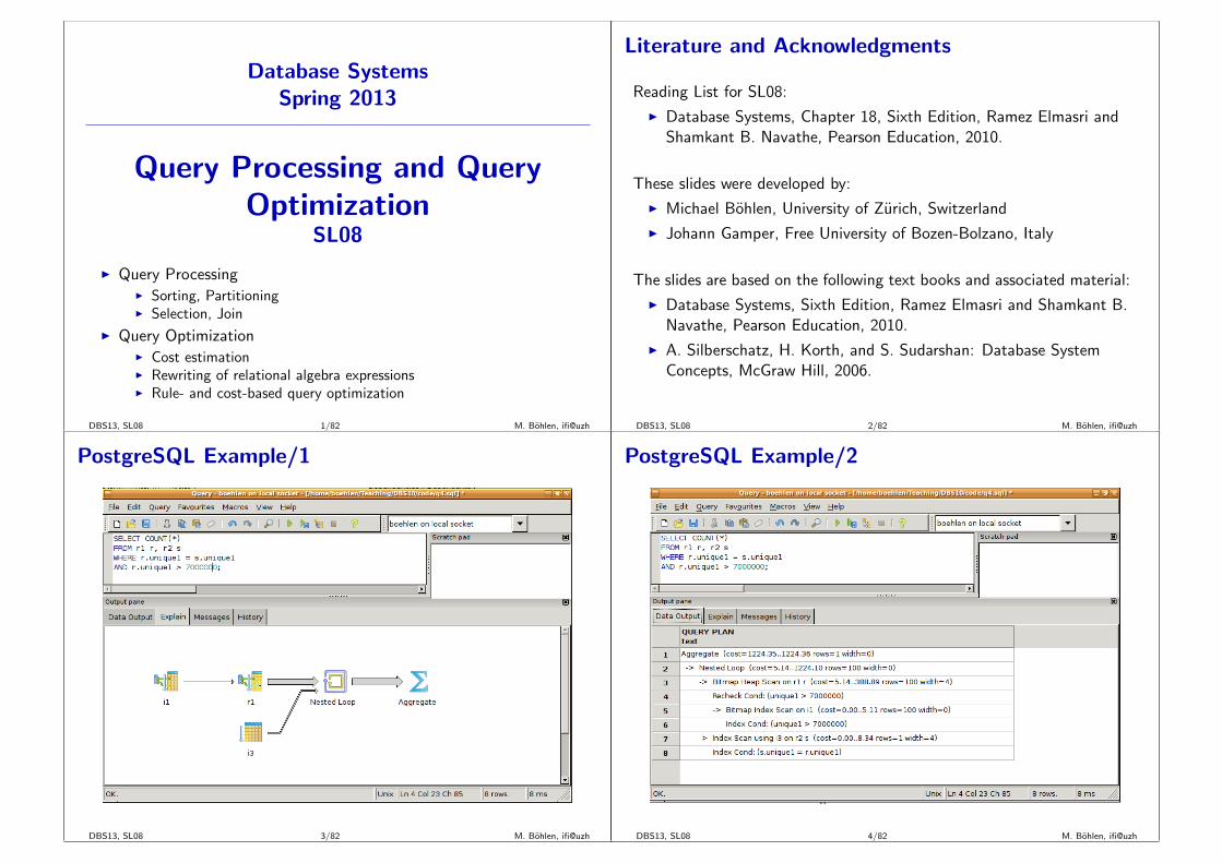
PostgreSQL Example/1
DBS13, SL08 3/82 M. Bohlen, ifi@uzh
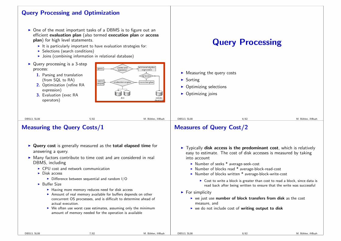
PostgreSQL Example/2
DBS13, SL08 4/82 M. Bohlen, ifi@uzh
Query Processing and Optimization
I One of the most important tasks of a DBMS is to figure out anefficient evaluation plan (also termed execution plan or accessplan) for high level statements.
I It is particularly important to have evaluation strategies for:I Selections (search conditions)I Joins (combining information in relational database)
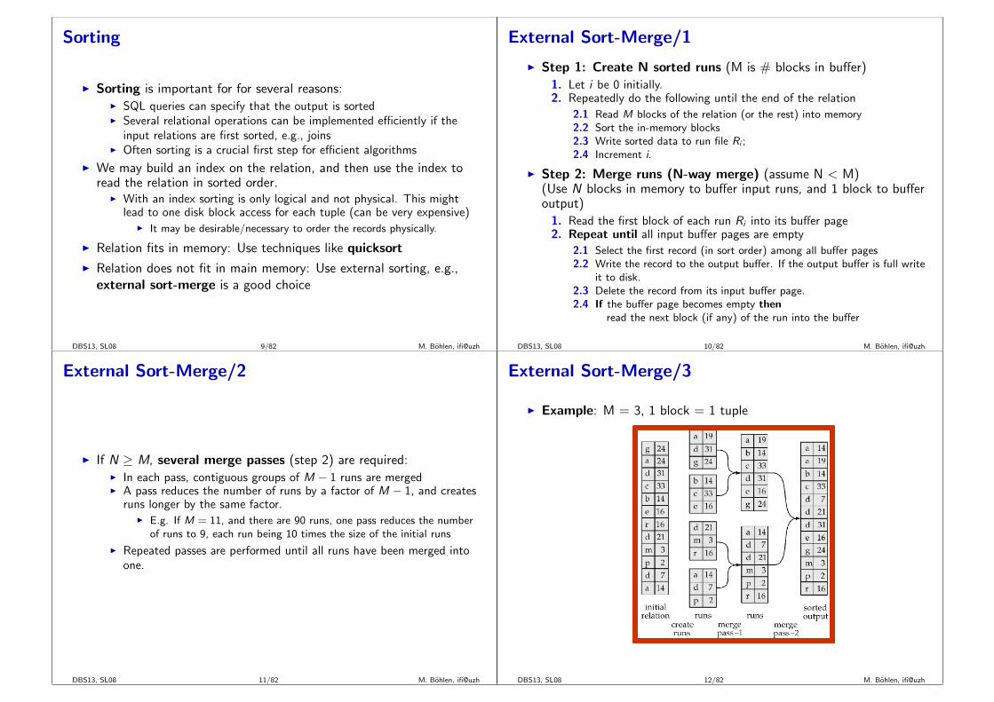
I Query processing is a 3-stepprocess:
1. Parsing and translation(from SQL to RA)
2. Optimization (refine RAexpression)
3. Evaluation (exec RAoperators)
DBS13, SL08 5/82 M. Bohlen, ifi@uzh
Query Processing
I Measuring the query costs
I Sorting
I Optimizing selections
I Optimizing joins
DBS13, SL08 6/82 M. Bohlen, ifi@uzh
Measuring the Query Costs/1
I Query cost is generally measured as the total elapsed time foranswering a query.
I Many factors contribute to time cost and are considered in realDBMS, including
I CPU cost and network communicationI Disk access
I Difference between sequential and random I/O
I Buffer SizeI Having more memory reduces need for disk accessI Amount of real memory available for buffers depends on other
concurrent OS procsesses, and is difficult to determine ahead ofactual execution.
I We often use worst case estimates, assuming only the minimumamount of memory needed for the operation is available
DBS13, SL08 7/82 M. Bohlen, ifi@uzh
Measures of Query Cost/2
I Typically disk access is the predominant cost, which is relativelyeasy to estimate. The cost of disk accesses is measured by takinginto account
I Number of seeks * average-seek-costI Number of blocks read * average-block-read-costI Number of blocks written * average-block-write-cost
I Cost to write a block is greater than cost to read a block, since data isread back after being written to ensure that the write was successful
I For simplicityI we just use number of block transfers from disk as the cost
measure, andI we do not include cost of writing output to disk
DBS13, SL08 8/82 M. Bohlen, ifi@uzh
Sorting
I Sorting is important for for several reasons:I SQL queries can specify that the output is sortedI Several relational operations can be implemented efficiently if the
input relations are first sorted, e.g., joinsI Often sorting is a crucial first step for efficient algorithms
I We may build an index on the relation, and then use the index toread the relation in sorted order.
I With an index sorting is only logical and not physical. This mightlead to one disk block access for each tuple (can be very expensive)
I It may be desirable/necessary to order the records physically.
I Relation fits in memory: Use techniques like quicksort
I Relation does not fit in main memory: Use external sorting, e.g.,external sort-merge is a good choice
DBS13, SL08 9/82 M. Bohlen, ifi@uzh
External Sort-Merge/1
I Step 1: Create N sorted runs (M is # blocks in buffer)
1. Let i be 0 initially.2. Repeatedly do the following until the end of the relation
2.1 Read M blocks of the relation (or the rest) into memory2.2 Sort the in-memory blocks2.3 Write sorted data to run file Ri ;2.4 Increment i.
I Step 2: Merge runs (N-way merge) (assume N < M)(Use N blocks in memory to buffer input runs, and 1 block to bufferoutput)
1. Read the first block of each run Ri into its buffer page2. Repeat until all input buffer pages are empty
2.1 Select the first record (in sort order) among all buffer pages2.2 Write the record to the output buffer. If the output buffer is full write
it to disk.2.3 Delete the record from its input buffer page.2.4 If the buffer page becomes empty then
read the next block (if any) of the run into the buffer
DBS13, SL08 10/82 M. Bohlen, ifi@uzh
External Sort-Merge/2
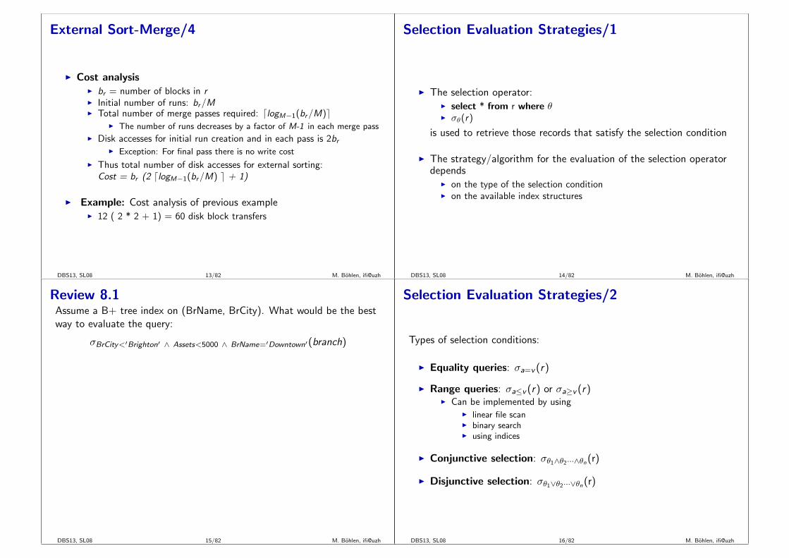
I If N ≥ M, several merge passes (step 2) are required:I In each pass, contiguous groups of M − 1 runs are mergedI A pass reduces the number of runs by a factor of M − 1, and creates
runs longer by the same factor.I E.g. If M = 11, and there are 90 runs, one pass reduces the number
of runs to 9, each run being 10 times the size of the initial runs
I Repeated passes are performed until all runs have been merged intoone.
DBS13, SL08 11/82 M. Bohlen, ifi@uzh
External Sort-Merge/3
I Example: M = 3, 1 block = 1 tuple
DBS13, SL08 12/82 M. Bohlen, ifi@uzh
External Sort-Merge/4
I Cost analysisI br = number of blocks in rI Initial number of runs: br/MI Total number of merge passes required: dlogM−1(br/M)e
I The number of runs decreases by a factor of M-1 in each merge pass
I Disk accesses for initial run creation and in each pass is 2brI Exception: For final pass there is no write cost
I Thus total number of disk accesses for external sorting:Cost = br (2 dlogM−1(br/M) e + 1)
I Example: Cost analysis of previous exampleI 12 ( 2 * 2 + 1) = 60 disk block transfers
DBS13, SL08 13/82 M. Bohlen, ifi@uzh
Selection Evaluation Strategies/1
I The selection operator:I select * from r where θI σθ(r)
is used to retrieve those records that satisfy the selection condition
I The strategy/algorithm for the evaluation of the selection operatordepends
I on the type of the selection conditionI on the available index structures
DBS13, SL08 14/82 M. Bohlen, ifi@uzh
Review 8.1Assume a B+ tree index on (BrName, BrCity). What would be the bestway to evaluate the query:
σBrCity<′Brighton′ ∧ Assets<5000 ∧ BrName=′Downtown′(branch)
DBS13, SL08 15/82 M. Bohlen, ifi@uzh
Selection Evaluation Strategies/2
Types of selection conditions:
I Equality queries: σa=v (r)
I Range queries: σa≤v (r) or σa≥v (r)I Can be implemented by using
I linear file scanI binary searchI using indices
I Conjunctive selection: σθ1∧θ2···∧θn(r)
I Disjunctive selection: σθ1∨θ2···∨θn(r)
DBS13, SL08 16/82 M. Bohlen, ifi@uzh
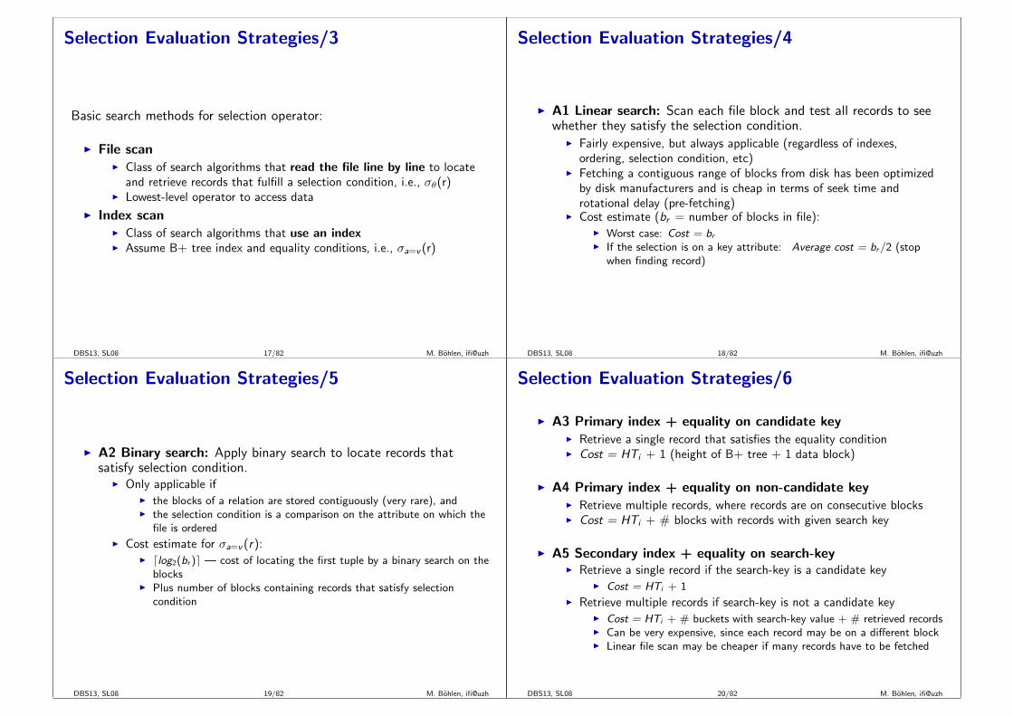
Selection Evaluation Strategies/3
Basic search methods for selection operator:
I File scanI Class of search algorithms that read the file line by line to locate
and retrieve records that fulfill a selection condition, i.e., σθ(r)I Lowest-level operator to access data
I Index scanI Class of search algorithms that use an indexI Assume B+ tree index and equality conditions, i.e., σa=v (r)
DBS13, SL08 17/82 M. Bohlen, ifi@uzh
Selection Evaluation Strategies/4
I A1 Linear search: Scan each file block and test all records to seewhether they satisfy the selection condition.
I Fairly expensive, but always applicable (regardless of indexes,ordering, selection condition, etc)
I Fetching a contiguous range of blocks from disk has been optimizedby disk manufacturers and is cheap in terms of seek time androtational delay (pre-fetching)
I Cost estimate (br = number of blocks in file):I Worst case: Cost = brI If the selection is on a key attribute: Average cost = br/2 (stop
when finding record)
DBS13, SL08 18/82 M. Bohlen, ifi@uzh
Selection Evaluation Strategies/5
I A2 Binary search: Apply binary search to locate records thatsatisfy selection condition.
I Only applicable ifI the blocks of a relation are stored contiguously (very rare), andI the selection condition is a comparison on the attribute on which the
file is ordered
I Cost estimate for σa=v (r):I dlog2(br )e — cost of locating the first tuple by a binary search on the
blocksI Plus number of blocks containing records that satisfy selection
condition
DBS13, SL08 19/82 M. Bohlen, ifi@uzh
Selection Evaluation Strategies/6
I A3 Primary index + equality on candidate keyI Retrieve a single record that satisfies the equality conditionI Cost = HTi + 1 (height of B+ tree + 1 data block)
I A4 Primary index + equality on non-candidate keyI Retrieve multiple records, where records are on consecutive blocksI Cost = HTi + # blocks with records with given search key
I A5 Secondary index + equality on search-keyI Retrieve a single record if the search-key is a candidate key
I Cost = HTi + 1
I Retrieve multiple records if search-key is not a candidate keyI Cost = HTi + # buckets with search-key value + # retrieved recordsI Can be very expensive, since each record may be on a different blockI Linear file scan may be cheaper if many records have to be fetched
DBS13, SL08 20/82 M. Bohlen, ifi@uzh
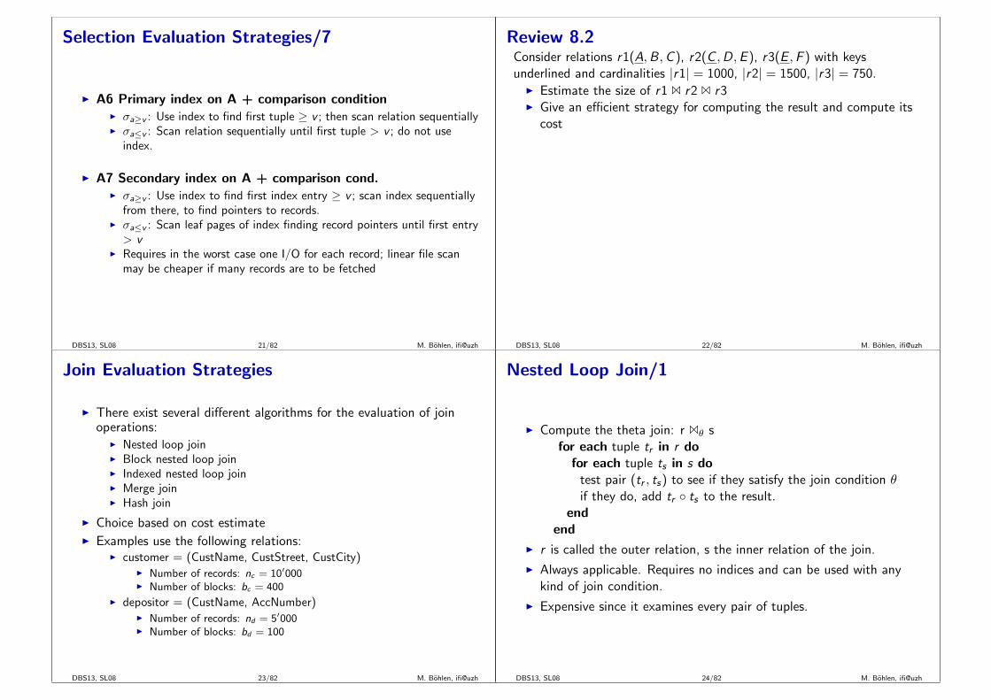
Selection Evaluation Strategies/7
I A6 Primary index on A + comparison conditionI σa≥v : Use index to find first tuple ≥ v ; then scan relation sequentiallyI σa≤v : Scan relation sequentially until first tuple > v ; do not use
index.
I A7 Secondary index on A + comparison cond.I σa≥v : Use index to find first index entry ≥ v ; scan index sequentially
from there, to find pointers to records.I σa≤v : Scan leaf pages of index finding record pointers until first entry> v
I Requires in the worst case one I/O for each record; linear file scanmay be cheaper if many records are to be fetched
DBS13, SL08 21/82 M. Bohlen, ifi@uzh
Review 8.2Consider relations r1(A,B,C ), r2(C ,D,E ), r3(E ,F ) with keysunderlined and cardinalities |r1| = 1000, |r2| = 1500, |r3| = 750.
I Estimate the size of r1 1 r2 1 r3I Give an efficient strategy for computing the result and compute its
cost
DBS13, SL08 22/82 M. Bohlen, ifi@uzh
Join Evaluation Strategies
I There exist several different algorithms for the evaluation of joinoperations:
I Nested loop joinI Block nested loop joinI Indexed nested loop joinI Merge joinI Hash join
I Choice based on cost estimateI Examples use the following relations:
I customer = (CustName, CustStreet, CustCity)I Number of records: nc = 10′000I Number of blocks: bc = 400
I depositor = (CustName, AccNumber)I Number of records: nd = 5′000I Number of blocks: bd = 100
DBS13, SL08 23/82 M. Bohlen, ifi@uzh
Nested Loop Join/1
I Compute the theta join: r 1θ sfor each tuple tr in r do
for each tuple ts in s dotest pair (tr , ts) to see if they satisfy the join condition θif they do, add tr ◦ ts to the result.
endend
I r is called the outer relation, s the inner relation of the join.
I Always applicable. Requires no indices and can be used with anykind of join condition.
I Expensive since it examines every pair of tuples.
DBS13, SL08 24/82 M. Bohlen, ifi@uzh
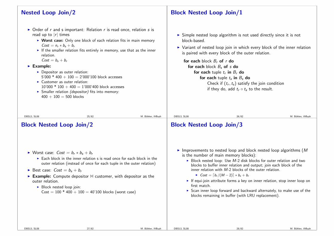
Nested Loop Join/2
I Order of r and s important: Relation r is read once, relation s isread up to |r | times
I Worst case: Only one block of each relation fits in main memoryCost = nr ∗ bs + br
I If the smaller relation fits entirely in memory, use that as the innerrelation.Cost = bs + br
I Example:I Depositor as outer relation:
5’000 * 400 + 100 = 2’000’100 block accessesI Customer as outer relation:
10’000 * 100 + 400 = 1’000’400 block accessesI Smaller relation (depositor) fits into memory:
400 + 100 = 500 blocks
DBS13, SL08 25/82 M. Bohlen, ifi@uzh
Block Nested Loop Join/1
I Simple nested loop algorithm is not used directly since it is notblock-based.
I Variant of nested loop join in which every block of the inner relationis paired with every block of the outer relation.
for each block Br of r dofor each block Bs of s do
for each tuple tr in Br dofor each tuple ts in Bs do
Check if (tr , ts) satisfy the join conditionif they do, add tr ◦ ts to the result.
DBS13, SL08 26/82 M. Bohlen, ifi@uzh
Block Nested Loop Join/2
I Worst case: Cost = br ∗ bs + brI Each block in the inner relation s is read once for each block in the
outer relation (instead of once for each tuple in the outer relation)
I Best case: Cost = bs + brI Example: Compute depositor 1 customer, with depositor as the
outer relation.I Block nested loop join:
Cost = 100 * 400 + 100 = 40’100 blocks (worst case)
DBS13, SL08 27/82 M. Bohlen, ifi@uzh
Block Nested Loop Join/3
I Improvements to nested loop and block nested loop algorithms (Mis the number of main memory blocks):
I Block nested loop: Use M-2 disk blocks for outer relation and twoblocks to buffer inner relation and output; join each block of theinner relation with M-2 blocks of the outer relation.
I Cost = dbr/(M − 2)e ∗ bs + br
I If equi-join attribute forms a key on inner relation, stop inner loop onfirst match.
I Scan inner loop forward and backward alternately, to make use of theblocks remaining in buffer (with LRU replacement).
DBS13, SL08 28/82 M. Bohlen, ifi@uzh
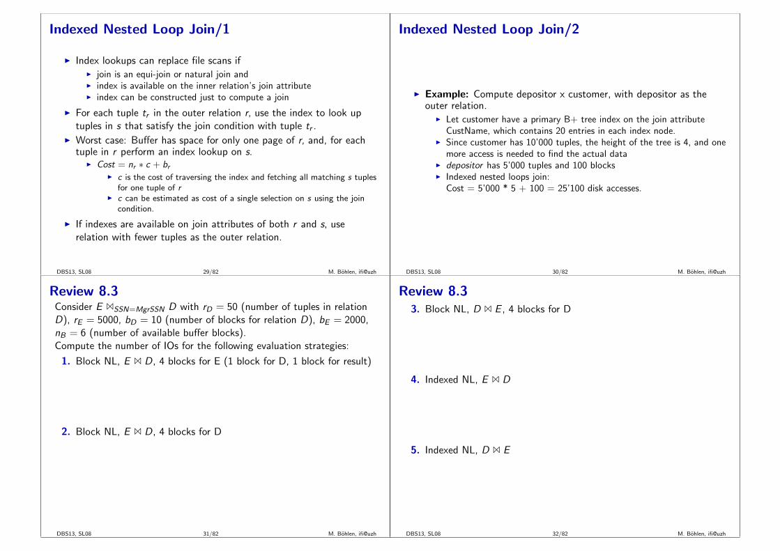
Indexed Nested Loop Join/1
I Index lookups can replace file scans ifI join is an equi-join or natural join andI index is available on the inner relation’s join attributeI index can be constructed just to compute a join
I For each tuple tr in the outer relation r, use the index to look uptuples in s that satisfy the join condition with tuple tr .
I Worst case: Buffer has space for only one page of r, and, for eachtuple in r perform an index lookup on s.
I Cost = nr ∗ c + brI c is the cost of traversing the index and fetching all matching s tuples
for one tuple of rI c can be estimated as cost of a single selection on s using the join
condition.
I If indexes are available on join attributes of both r and s, userelation with fewer tuples as the outer relation.
DBS13, SL08 29/82 M. Bohlen, ifi@uzh
Indexed Nested Loop Join/2
I Example: Compute depositor x customer, with depositor as theouter relation.
I Let customer have a primary B+ tree index on the join attributeCustName, which contains 20 entries in each index node.
I Since customer has 10’000 tuples, the height of the tree is 4, and onemore access is needed to find the actual data
I depositor has 5’000 tuples and 100 blocksI Indexed nested loops join:
Cost = 5’000 * 5 + 100 = 25’100 disk accesses.
DBS13, SL08 30/82 M. Bohlen, ifi@uzh
Review 8.3Consider E 1SSN=MgrSSN D with rD = 50 (number of tuples in relationD), rE = 5000, bD = 10 (number of blocks for relation D), bE = 2000,nB = 6 (number of available buffer blocks).Compute the number of IOs for the following evaluation strategies:
1. Block NL, E 1 D, 4 blocks for E (1 block for D, 1 block for result)
2. Block NL, E 1 D, 4 blocks for D
DBS13, SL08 31/82 M. Bohlen, ifi@uzh
Review 8.33. Block NL, D 1 E , 4 blocks for D
4. Indexed NL, E 1 D
5. Indexed NL, D 1 E
DBS13, SL08 32/82 M. Bohlen, ifi@uzh
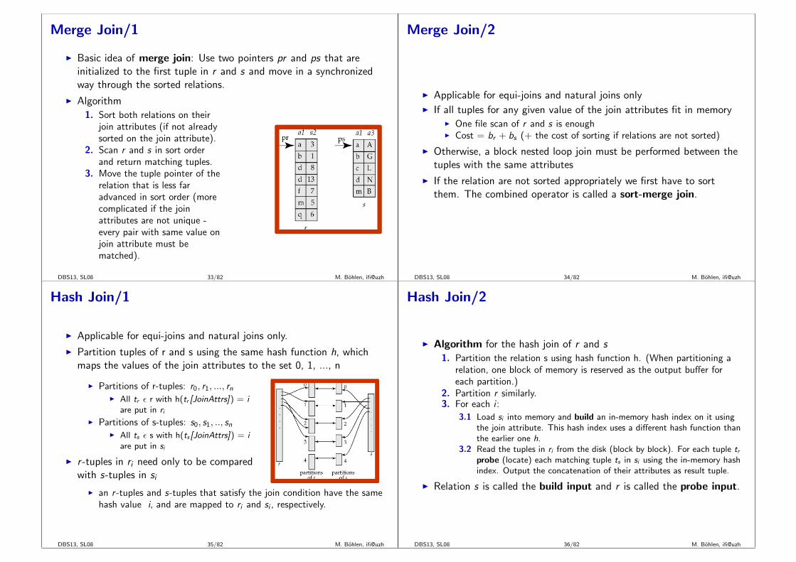
Merge Join/1
I Basic idea of merge join: Use two pointers pr and ps that areinitialized to the first tuple in r and s and move in a synchronizedway through the sorted relations.
I Algorithm
1. Sort both relations on theirjoin attributes (if not alreadysorted on the join attribute).
2. Scan r and s in sort orderand return matching tuples.
3. Move the tuple pointer of therelation that is less faradvanced in sort order (morecomplicated if the joinattributes are not unique -every pair with same value onjoin attribute must bematched).
DBS13, SL08 33/82 M. Bohlen, ifi@uzh
Merge Join/2
I Applicable for equi-joins and natural joins onlyI If all tuples for any given value of the join attributes fit in memory
I One file scan of r and s is enoughI Cost = br + bs (+ the cost of sorting if relations are not sorted)
I Otherwise, a block nested loop join must be performed between thetuples with the same attributes
I If the relation are not sorted appropriately we first have to sortthem. The combined operator is called a sort-merge join.
DBS13, SL08 34/82 M. Bohlen, ifi@uzh
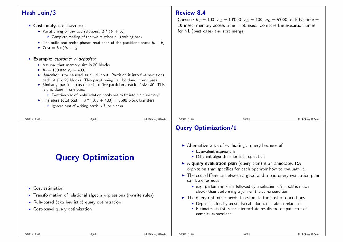
Hash Join/1
I Applicable for equi-joins and natural joins only.
I Partition tuples of r and s using the same hash function h, whichmaps the values of the join attributes to the set 0, 1, ..., n
I Partitions of r-tuples: r0, r1, ..., rnI All tr ε r with h(tr [JoinAttrs]) = i
are put in riI Partitions of s-tuples: s0, s1, .., sn
I All ts ε s with h(ts [JoinAttrs]) = iare put in si
I r -tuples in ri need only to be comparedwith s-tuples in si
I an r -tuples and s-tuples that satisfy the join condition have the samehash value i, and are mapped to ri and si , respectively.
DBS13, SL08 35/82 M. Bohlen, ifi@uzh
Hash Join/2
I Algorithm for the hash join of r and s
1. Partition the relation s using hash function h. (When partitioning arelation, one block of memory is reserved as the output buffer foreach partition.)
2. Partition r similarly.3. For each i :
3.1 Load si into memory and build an in-memory hash index on it usingthe join attribute. This hash index uses a different hash function thanthe earlier one h.
3.2 Read the tuples in ri from the disk (block by block). For each tuple trprobe (locate) each matching tuple ts in si using the in-memory hashindex. Output the concatenation of their attributes as result tuple.
I Relation s is called the build input and r is called the probe input.
DBS13, SL08 36/82 M. Bohlen, ifi@uzh
Hash Join/3
I Cost analysis of hash joinI Partitioning of the two relations: 2 * (br + bs)
I Complete reading of the two relations plus writing back
I The build and probe phases read each of the partitions once: br + bsI Cost = 3 ∗ (br + bs)
I Example: customer 1 depositorI Assume that memory size is 20 blocksI bd = 100 and bc = 400.I depositor is to be used as build input. Partition it into five partitions,
each of size 20 blocks. This partitioning can be done in one pass.I Similarly, partition customer into five partitions, each of size 80. This
is also done in one pass.I Partition size of probe relation needs not to fit into main memory!
I Therefore total cost = 3 * (100 + 400) = 1500 block transfersI Ignores cost of writing partially filled blocks
DBS13, SL08 37/82 M. Bohlen, ifi@uzh
Review 8.4Consider bC = 400, nC = 10′000, bD = 100, nD = 5′000, disk IO time =10 msec, memory access time = 60 nsec. Compare the execution timesfor NL (best case) and sort merge.
DBS13, SL08 38/82 M. Bohlen, ifi@uzh
Query Optimization
I Cost estimation
I Transformation of relational algebra expressions (rewrite rules)
I Rule-based (aka heuristic) query optimization
I Cost-based query optimization
DBS13, SL08 39/82 M. Bohlen, ifi@uzh
Query Optimization/1
I Alternative ways of evaluating a query because ofI Equivalent expressionsI Different algorithms for each operation
I A query evaluation plan (query plan) is an annotated RAexpression that specifies for each operator how to evaluate it.
I The cost difference between a good and a bad query evaluation plancan be enormous
I e.g., performing r × s followed by a selection r.A = s.B is muchslower than performing a join on the same condition
I The query optimizer needs to estimate the cost of operationsI Depends critically on statistical information about relationsI Estimates statistics for intermediate results to compute cost of
complex expressions
DBS13, SL08 40/82 M. Bohlen, ifi@uzh
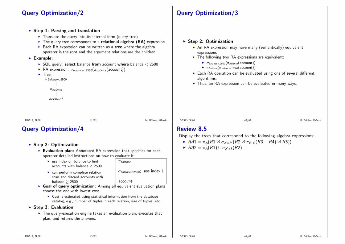
Query Optimization/2
I Step 1: Parsing and translationI Translate the query into its internal form (query tree)I The query tree corresponds to a relational algebra (RA) expressionI Each RA expression can be written as a tree where the algebra
operator is the root and the argument relations are the children.
I Example:I SQL query: select balance from account where balance < 2500I RA expression: σbalance<2500(πbalance(account))I Tree:
σbalance<2500
|πbalance|
account
DBS13, SL08 41/82 M. Bohlen, ifi@uzh
Query Optimization/3
I Step 2: OptimizationI An RA expression may have many (semantically) equivalent
expressionsI The following two RA expressions are equivalent:
I σbalance<2500(πbalance(account))I πbalance(σbalance<2500(account))
I Each RA operation can be evaluated using one of several differentalgorithms.
I Thus, an RA expression can be evaluated in many ways.
DBS13, SL08 42/82 M. Bohlen, ifi@uzh
Query Optimization/4
I Step 2: OptimizationI Evaluation plan: Annotated RA expression that specifies for each
operator detailed instructions on how to evaluate it.I use index on balance to find
accounts with balance < 2500
I can perform complete relationscan and discard accounts withbalance ≥ 2500
πbalance|σbalance<2500; use index 1|account
I Goal of query optimization: Among all equivalent evaluation planschoose the one with lowest cost.
I Cost is estimated using statistical information from the databasecatalog, e.g., number of tuples in each relation, size of tuples, etc.
I Step 3: EvaluationI The query-execution engine takes an evaluation plan, executes that
plan, and returns the answers.
DBS13, SL08 43/82 M. Bohlen, ifi@uzh
Review 8.5Display the trees that correspond to the following algebra expressions:
I RA1 = πA(R1 1 σX=Y (R2 1 πB,C (R3− R4) 1 R5))I RA2 = πA(R1) ∪ σX>5(R2)
DBS13, SL08 44/82 M. Bohlen, ifi@uzh
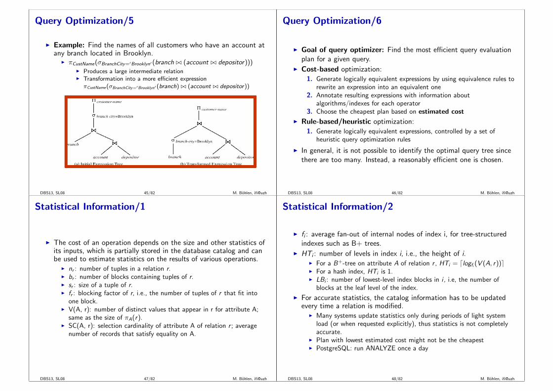
Query Optimization/5
I Example: Find the names of all customers who have an account atany branch located in Brooklyn.
I πCustName(σBranchCity=′Brooklyn′(branch ./ (account ./ depositor)))I Produces a large intermediate relationI Transformation into a more efficient expressionπCustName(σBranchCity=′Brooklyn′(branch) ./ (account ./ depositor))
DBS13, SL08 45/82 M. Bohlen, ifi@uzh
Query Optimization/6
I Goal of query optimizer: Find the most efficient query evaluationplan for a given query.
I Cost-based optimization:
1. Generate logically equivalent expressions by using equivalence rules torewrite an expression into an equivalent one
2. Annotate resulting expressions with information aboutalgorithms/indexes for each operator
3. Choose the cheapest plan based on estimated cost
I Rule-based/heuristic optimization:
1. Generate logically equivalent expressions, controlled by a set ofheuristic query optimization rules
I In general, it is not possible to identify the optimal query tree sincethere are too many. Instead, a reasonably efficient one is chosen.
DBS13, SL08 46/82 M. Bohlen, ifi@uzh
Statistical Information/1
I The cost of an operation depends on the size and other statistics ofits inputs, which is partially stored in the database catalog and canbe used to estimate statistics on the results of various operations.
I nr : number of tuples in a relation r.I br : number of blocks containing tuples of r.I sr : size of a tuple of r.I fr : blocking factor of r, i.e., the number of tuples of r that fit into
one block.I V(A, r): number of distinct values that appear in r for attribute A;
same as the size of πA(r).I SC(A, r): selection cardinality of attribute A of relation r ; average
number of records that satisfy equality on A.
DBS13, SL08 47/82 M. Bohlen, ifi@uzh
Statistical Information/2
I fi : average fan-out of internal nodes of index i, for tree-structuredindexes such as B+ trees.
I HTi : number of levels in index i, i.e., the height of i.I For a B+-tree on attribute A of relation r , HTi = dlogfi (V (A, r))eI For a hash index, HTi is 1.I LBi : number of lowest-level index blocks in i , i.e, the number of
blocks at the leaf level of the index.
I For accurate statistics, the catalog information has to be updatedevery time a relation is modified.
I Many systems update statistics only during periods of light systemload (or when requested explicitly), thus statistics is not completelyaccurate.
I Plan with lowest estimated cost might not be the cheapestI PostgreSQL: run ANALYZE once a day
DBS13, SL08 48/82 M. Bohlen, ifi@uzh
Rewriting Relational Algebra Expressions
I Two relational algebra expressions are equivalent if on every legaldatabase instance the two expressions generate the same set oftuples
I Note: order of tuples is irrelevant
I Two expressions in the multiset version of the relational algebra aresaid to be equivalent if on every legal database instance the twoexpressions generate the same multiset of tuples
I An equivalence rule states that two different expressions areequivalent and can replace each other
DBS13, SL08 49/82 M. Bohlen, ifi@uzh
Equivalence Rules/1
I E ,E1, . . . = RA expressionsθ, θ1, . . . = predicates/conditions
I ER1 Conjunctive selection operations can be deconstructed into asequence of individual selections.
σθ1∧θ2 (E ) = σθ1 (σθ2 (E ))
I ER2 Selection operations are commutative.σθ1 (σθ2 (E )) = σθ2 (σθ1 (E ))
I ER3 Only the last in a sequence of projections is needed, the otherscan be omitted (Li are lists of attributes).
πL1(πL2(. . . (πLn(E )) . . . )) = πL1(E )
I ER4 Selections can be combined with Cartesian product and thetajoins(a) σθ(E1 x E2) = E1 ./θ E2
(b) σθ1(E1 ./θ2 E2) = E1 ./θ1∧θ2 E2
DBS13, SL08 50/82 M. Bohlen, ifi@uzh
Equivalence Rules/2
I ER5 Theta joins (and natural joins) are commutative.E1 ./θ E2 = E2 ./θ E1
I ER6 Associativity(a) Natural join operations are associative:
(E1 ./ E2) ./ E3 = E1 ./ (E2 ./ E3)(b) Theta joins are associative in the following way:
(E1 ./θ1 E2) ./θ2∧θ3 E3 = E1 ./θ1∧θ3 (E2 ./θ2 E3)where θ2 involves attributes from only E2 and E3.Any of these conditions might be empty, hence, the Cartesian
product operation is also associative
I Commutativity and associativity of join operations are important forjoin reordering.
DBS13, SL08 51/82 M. Bohlen, ifi@uzh
Equivalence Rules/3
I ER7 The selection operation distributes over the theta joinoperation under the following conditions:
I (a) When all attributes in θo involve only the attributes of one of theexpressions (E1) being joined:
σθo (E1 ./θ E2) = σθo (E1) ./θ E2
I (b) When θ1 involves only the attributes of E1 and θ2 involves onlythe attributes of E2:
σθ1∧θ2(E1 ./θ E2) = σθ1(E1) ./θ σθ2(E2)
DBS13, SL08 52/82 M. Bohlen, ifi@uzh
Equivalence Rules/4
I ER8 The projection operation distributes over the theta joinoperation as follows:
I Let L1 and L2 be sets of attributes from E1 and E2, respectively.
I (a) if θ involves only attributes from L1 ∪ L2:πL1∪L2 (E1 1θ E2) = πL1 (E1) 1θ πL2 (E2)
I (b) Consider a join E1 1θ E2.I Let L3 be attributes of E1 that are involved in join condition θ, but
are not in L1 ∪ L2, andI Let L4 be attributes of E2 that are involved in join condition θ, but
are not in L1 ∪ L2, andπL1∪L2 (E1 1θ E2) = πL1∪L2 (πL1∪L3 (E1) 1θ πL2∪L4 (E2))
DBS13, SL08 53/82 M. Bohlen, ifi@uzh
Equivalence Rules/5
I ER9 The set operations union and intersection are commutativeE1 ∪ E2 = E2 ∪ E1
E1 ∩ E2 = E2 ∩ E1
Set difference is not commutative
I ER10 Set union and intersection are associative.(E1 ∪ E2) ∪ E3 = E1 ∪ (E2 ∪ E3)(E1 ∩ E2) ∩ E3 = E1 ∩ (E2 ∩ E3)
DBS13, SL08 54/82 M. Bohlen, ifi@uzh
Equivalence Rules/6
I ER11 The selection operation distributes over ∪,∩ and −.σθ(E1 − E2) = σθ(E1)− σθ(E2)σθ(E1 ∪ E2) = σθ(E1) ∪ σθ(E2)σθ(E1 ∩ E2) = σθ(E1) ∩ σθ(E2)
Also σθ(E1 − E2) = σθ(E1)− E2
and similarly for ∩ in place of −, but not for ∪
I ER12 The projection operation distributes over unionπL(E1 ∪ E2) = πL(E ) ∪ πL(E2)
DBS13, SL08 55/82 M. Bohlen, ifi@uzh
Review 8.6Determine the equivalences that hold. Give counterexamples for the falseones.
1. σθ(XϑF (A)) = XϑF (σθ(A)), attr(θ) ⊆ attr(X )
2. πX (A− B) = πX (A)− πX (B)
3. A d|><| (B d|><|C ) = (A d|><|B) d|><|C
4. A ∩ B = A ∪ B − (A− B)− (B − A)
DBS13, SL08 56/82 M. Bohlen, ifi@uzh
Rewrite Examples/1
I Example 1: Bank databaseI branch = (BranchName, BranchCity, Assets)I account = (AccNumber, BranchName, Balance)I depositor = (CustName, AccNumber)
I Query: Find the names of all customers who have an account atsome branch located in Brooklyn.πCustName(σBranchCity=′Brooklyn′(branch 1 (account 1 depositor)))
I Transformation using rule ER7(a):πCustName
(σBranchCity=′Brooklyn′(branch) 1 (account 1 depositor))
I Performing the selection as early as possible reduces the size of theintermediate relation to be joined.
DBS13, SL08 57/82 M. Bohlen, ifi@uzh
Rewrite Examples/2
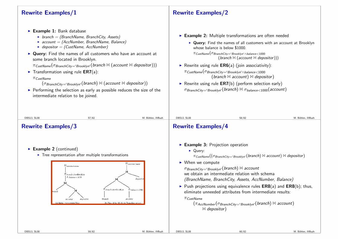
I Example 2: Multiple transformations are often needed
I Query: Find the names of all customers with an account at Brooklynwhose balance is below $1000.πCustName(σBranchCity=′Brooklyn′∧balance<1000
(branch 1 (account 1 depositor)))
I Rewrite using rule ER6(a) (join associativity):πCustName(σBranchCity=′Brooklyn′∧balance<1000
(branch 1 account) 1 depositor)
I Rewrite using rule ER7(b) (perform selection early)σBranchCity=′Brooklyn′(branch) 1 σbalance<1000(account)
DBS13, SL08 58/82 M. Bohlen, ifi@uzh
Rewrite Examples/3
I Example 2 (continued)I Tree representation after multiple transformations
DBS13, SL08 59/82 M. Bohlen, ifi@uzh
Rewrite Examples/4
I Example 3: Projection operationI Query:πCustName((σBranchCity=′Brooklyn′(branch) 1 account) 1 depositor)
I When we computeσBranchCity=′Brooklyn′(branch) 1 accountwe obtain an intermediate relation with schema(BranchName, BranchCity, Assets, AccNumber, Balance)
I Push projections using equivalence rules ER8(a) and ER8(b); thus,eliminate unneeded attributes from intermediate results:πCustName
(πAccNumber (σBranchCity=′Brooklyn′(branch) 1 account)1 depositor)
DBS13, SL08 60/82 M. Bohlen, ifi@uzh
Rewrite Examples/5
I Example 4: Join ordering
I For all relations r1, r2, and r3:(r1 1 r2) 1 r3 = r1 1 (r2 1 r3)
I If r2 1 r3 is quite large and r1 1 r2 is small, we choose(r1 1 r2) 1 r3
so that we compute and store a smaller temporary relation.
DBS13, SL08 61/82 M. Bohlen, ifi@uzh
Rewrite Examples/6
I Example 5: Join ordering
I Consider the expressionπCustName(σBranchCity=′Brooklyn′(branch) 1 account 1 depositor)
I Could compute account 1 depositor first, and join result withσBranchCity=′Brooklyn′(branch)
but account 1 depositor is likely to be a large relation.
I Since it is more likely that only a small fraction of the bank’scustomers have accounts in branches located in Brooklyn, it isbetter to compute first
σBranchCity=′Brooklyn′(branch) 1 account
DBS13, SL08 62/82 M. Bohlen, ifi@uzh
Review 8.7Show how to rewrite and optimize the following SQL query:
select E.LName
from Employee E, WorksOn W, Project P
where P.PName = ’A’
and P.PNum = W.PNo
and W.ESSN = E.SSN
and E.BDate = ’31.12.1957’
DBS13, SL08 63/82 M. Bohlen, ifi@uzh
Enumeration of Equivalent Expressions
I Query optimizers use the equivalence rules to systematicallygenerate expressions that are equivalent to the given expression
I repeatFor each expression found so far, use all applicableequivalence rules, and add newly generated expressionsto the set of expressions found so far
until no more expressions can be found
I This approach is very expensive in space and timeI Reduce space requirements by sharing common subexpressions:
I When E1 is generated from E2 by an equivalence rule, usually onlythe top level of the two are different, subtrees below are the same andcan be shared (e.g. when applying join associativity)
I Time requirements are reduced by not generating all expressions(e.g. take cost estimates into account)
DBS13, SL08 64/82 M. Bohlen, ifi@uzh
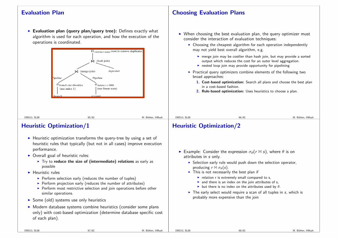
Evaluation Plan
I Evaluation plan (query plan/query tree): Defines exactly whatalgorithm is used for each operation, and how the execution of theoperations is coordinated.
DBS13, SL08 65/82 M. Bohlen, ifi@uzh
Choosing Evaluation Plans
I When choosing the best evaluation plan, the query optimizer mustconsider the interaction of evaluation techniques:
I Choosing the cheapest algorithm for each operation independentlymay not yield best overall algorithm, e.g.
I merge join may be costlier than hash join, but may provide a sortedoutput which reduces the cost for an outer level aggregation.
I nested loop join may provide opportunity for pipelining
I Practical query optimizers combine elements of the following twobroad approaches:
1. Cost-based optimization: Search all plans and choose the best planin a cost-based fashion.
2. Rule-based optimization: Uses heuristics to choose a plan.
DBS13, SL08 66/82 M. Bohlen, ifi@uzh
Heuristic Optimization/1
I Heuristic optimization transforms the query-tree by using a set ofheuristic rules that typically (but not in all cases) improve executionperformance.
I Overall goal of heuristic rules:I Try to reduce the size of (intermediate) relations as early as
possible
I Heuristic rulesI Perform selection early (reduces the number of tuples)I Perform projection early (reduces the number of attributes)I Perform most restrictive selection and join operations before other
similar operations.
I Some (old) systems use only heuristics
I Modern database systems combine heuristics (consider some plansonly) with cost-based optimization (determine database specific costof each plan).
DBS13, SL08 67/82 M. Bohlen, ifi@uzh
Heuristic Optimization/2
I Example: Consider the expression σθ(r 1 s), where θ is onattributes in s only.
I Selection early rule would push down the selection operator,producing r 1 σθ(s).
I This is not necessarily the best plan ifI relation r is extremely small compared to s,I and there is an index on the join attributes of s,I but there is no index on the attributes used by θ.
I The early select would require a scan of all tuples in s, which isprobably more expensive than the join
DBS13, SL08 68/82 M. Bohlen, ifi@uzh
Heuristic Optimization/3
I Steps in typical heuristic optimization
1. Break up conjunctive selections into a sequence of single selectionoperations (rule ER1).
2. Move selection operations down the query tree for the earliestpossible execution (rules ER2, ER7(a), ER7(b), ER11).
3. Execute first those selection and join operations that will produce thesmallest relations (rule ER6).
4. Replace Cartesian product operations that are followed by a selectioncondition by join operations (rule ER4(a)).
5. Deconstruct and move as far down the tree as possible lists ofprojection attributes, creating new projections where needed (rulesER3, ER8(a), ER8(b), ER12).
6. Identify those subtrees whose operations can be pipelined, andexecute them using pipelining.
DBS13, SL08 69/82 M. Bohlen, ifi@uzh
Cost-Based Optimization/1
Basic working of a cost-based query optimizer:I Algorithm
1. Use transformations (equivalence rules) to generate multiplecandidate evaluation plans from the original evaluation plan.
2. Cost formulas estimate the cost of executing each operation in eachcandidate evaluation plan.
I Cost formulas are parameterized by- statistics of the input relations;- dependent on the specific algorithm used by the operator;- CPU time, I/O time, communication time, main memory usage, ora combination.
3. The candidate evaluation plan with the least total cost is selectedfor execution.
DBS13, SL08 70/82 M. Bohlen, ifi@uzh
Cost-Based Optimization/2
I Cost-based optimization can be used to determine the best joinorder.
I A good ordering of joins is important for reducing the size oftemporary results (|r |, ..., |r |n).
I Consider finding the best join-order for r1 1 r2 1 ...rmI There are (2(m − 1))!/(m − 1)! different join orders for above
expression.I With m = 3, the number is 12I With m = 7, the number is 665,280I With m = 10, the number is greater than 17.6 billion
DBS13, SL08 71/82 M. Bohlen, ifi@uzh
Cost-Based Optimization/3
I Cost-based optimization is expensive, but worthwhile for queries onlarge datasets
I Typical queries have a small number m of operations; generallym<10
I With dynamic programming time complexity of optimization withbushy trees is O(3m).
I With m = 10, this number is 59000 instead of 17.6 billion!
I Space complexity is O(2m)
DBS13, SL08 72/82 M. Bohlen, ifi@uzh
Review 8.8Consider a DB with the following characteristics:
I |r1(A,B,C )| = 1000,V (C , r1) = 900I |r2(c ,D,E )| = 1500,V (C , r2) = 1100,V (E , r2) = 50I |r3(E ,F )| = 750,V (E , r3) = 100
Estimate the size of r1 1 r2 1 r3 and determine an efficient evaluationstrategy.
DBS13, SL08 73/82 M. Bohlen, ifi@uzh
Cost-Based Optimization Example/1
I Example: σSSN=0810643773(Emp)I Statistics:
I |Emp| = 10’000 tuplesI 5 tuples per blockI Secondary B+-tree index of depth 4 on SSNI SSN is primary key
I Plan p1: full table scanI cost(p1) = (10’000/5)/2 = 1’000 blocks
I Plan p2: B+-tree lookupI cost(p2) = 4 + 1 = 5 blocks
DBS13, SL08 74/82 M. Bohlen, ifi@uzh
Cost-Based Optimization Example/2
I Example: σDNo>15(Emp)I Statistics:
I |Emp| = 10’000 tuplesI 5 tuples per blockI Primary index on DNo of depth 2I 50 different departments
I Plan p1: full table scanI cost (p1) = 10’000/5 = 2’000 blocks
I Plan p2: index searchI cost(p2) = 2 + (50-15)/50*(10’000/5) = 1’400 blocks
DBS13, SL08 75/82 M. Bohlen, ifi@uzh
Cost-Based Optimization Example/3
I Emp 1DNo=DNum DeptI Statistics:
I |Emp| = 10’000 tuples ; 5 Emp tuples per blockI |Dept| = 125; 10 Dept tuples per blockI Hash index on Emp(DNo)I 4 EmpDept result tuples per block
I Plan p1: Block nested loop with Emp as outer loopI cost(p1) = (10’000/5) + (10’000/5) * (125/10) + (10’000/4)
= 30’500 IOsI (10.000/4 is cost of writing final output)
I Plan p2: Indexed nested loop with Dept as outer loop and hashedlookup in Emp
I cost(p2) = (125/10) + 125 * (10’000/125/5) + (10’000/4)= 4’513 IOs
I 10’000/125/5 is the average number of blocks/department
DBS13, SL08 76/82 M. Bohlen, ifi@uzh
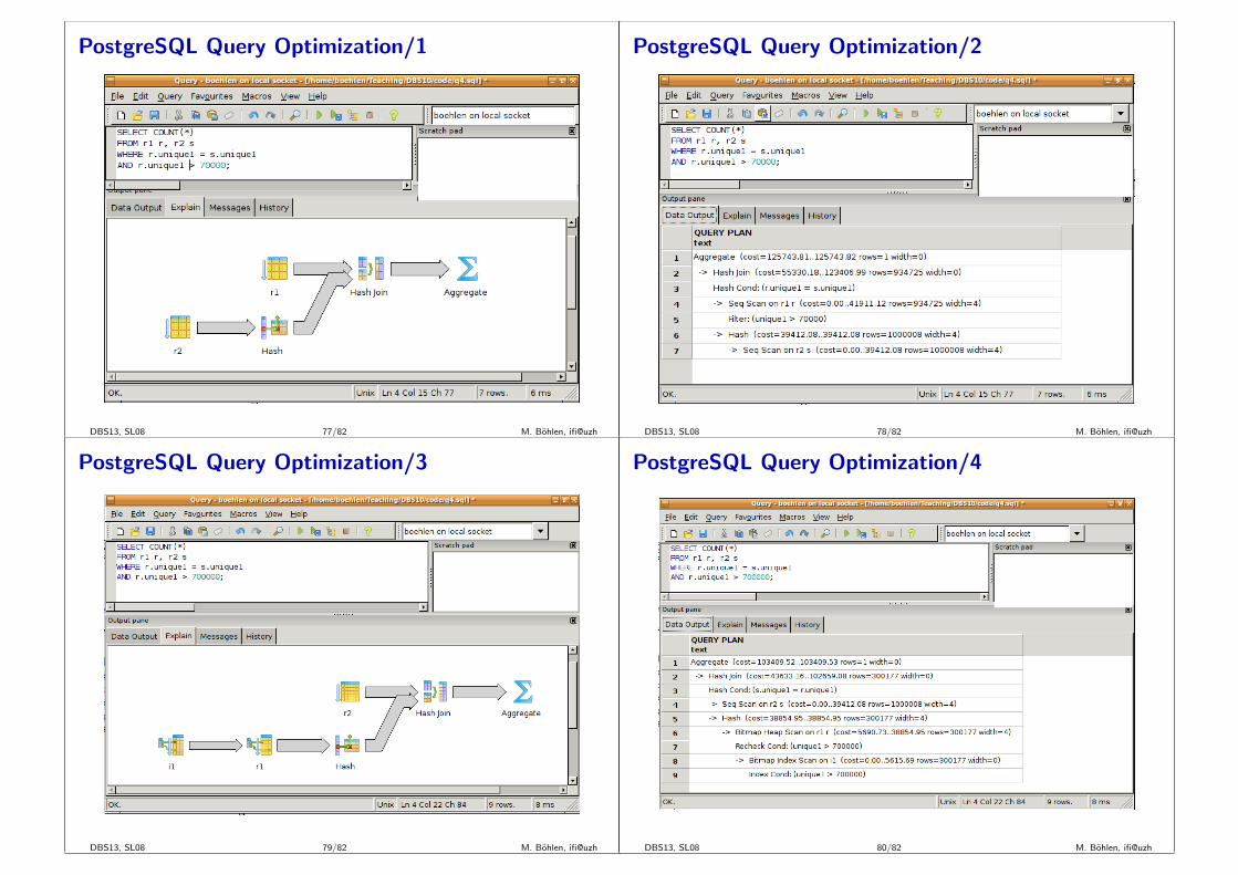
PostgreSQL Query Optimization/1
DBS13, SL08 77/82 M. Bohlen, ifi@uzh
PostgreSQL Query Optimization/2
DBS13, SL08 78/82 M. Bohlen, ifi@uzh
PostgreSQL Query Optimization/3
DBS13, SL08 79/82 M. Bohlen, ifi@uzh
PostgreSQL Query Optimization/4
DBS13, SL08 80/82 M. Bohlen, ifi@uzh
Summary/1
I Query evaluation techniques:
I Physical sorting:I Physical sorting is a basic and important techniqueI The same sort order should be useful to many operators and not just
one (global optimization versus local optimization)
I Evaluation techniques for selections:I Use primary index if available; secondary index is much worseI Equality conditions are selective and should be optimizedI Linear scan with sequential IO is the base line for selections
I Evaluation techniques for joins:I nested loop: base line; avoid whenever possibleI sort merge: robust and fastI hash join: fastest; only for equality
DBS13, SL08 81/82 M. Bohlen, ifi@uzh
Summary/2
I Query optimization techniques
I Equivalence rules for relational algebra expressions (must hold formultisets)
I Rule-based query optimization is based on heuristics (usually thegoal is to keep intermediate results as small as possible)
I Cost-based query optimization uses statistical information to findthe cheapest (or reasonably cheap) plan
DBS13, SL08 82/82 M. Bohlen, ifi@uzh
Related Documents