Quaternionic differential operators

arX

iv:m

ath-

ph/0

0050

23v3

8 A

ug 2

002

Journal of Mathematical Physics 42, 2236-2265 (2001)math-ph/0005023 ΣδΛ

QUATERNIONIC DIFFERENTIAL OPERATORS

Stefano De Leo1 a and Gisele Ducati1,2 b

1 Department of Applied Mathematics, University of CampinasPO Box 6065, SP 13083-970, Campinas, [email protected]

[email protected] Department of Mathematics, University of Parana

PO Box 19081, PR 81531-970, Curitiba, [email protected]

Accepted for publication in JMP: February 6, 2001

Abstract. Motivated by a quaternionic formulation of quantum mechanics, we discussquaternionic and complex linear differential equations. We touch only a few aspects ofthe mathematical theory, namely the resolution of the second order differential equationswith constant coefficients. We overcome the problems coming out from the loss of thefundamental theorem of the algebra for quaternions and propose a practical method tosolve quaternionic and complex linear second order differential equations with constantcoefficients. The resolution of the complex linear Schrodinger equation, in presence ofquaternionic potentials, represents an interesting application of the mathematical mate-rial discussed in this paper.

PACS. 02.10.Tq – 02.30.Hq – 02.30.Jr – 02.30.Tb – 03.65.-w

1 INTRODUCTION

There is a substantial literature analyzing the possibility to discuss quantum systems by adoptingquaternionic wave functions [1–14]. This research field has been attacked by a number of peopleleading to substantial progress. In the last years, many articles [15–31], review papers [32–34] andbooks [35–37] provided a detailed investigation of group theory, eigenvalue problem, scattering theory,relativistic wave equations, Lagrangian formalism and variational calculus within a quaternionic for-mulation of quantum mechanics and field theory. In this context, by observing that the formulation ofphysical problems in mathematical terms often requires the study of partial differential equations, wedevelop the necessary theory to solve quaternionic and complex linear differential equations. The maindifficulty in carrying out the solution of quaternionic differential equations is obviously representedby the non commutative nature of the quaternionic field. The standard methods of resolution breakdown and, consequently, we need to modify the classical approach. It is not our purpose to developa complete quaternionic theory of differential equations. This exceeds the scope of this paper. Themain objective is to include what seemed to be most important for an introduction to this subject.In particular, we restrict ourselves to second order differential equations and give a practical methodto solve such equations when quaternionic constant coefficients appear.

Some of the results given in this paper can be obtained by translation into a complex formal-ism [15, 16, 31]. Nevertheless, many subtleties of quaternionic calculus are often lost by using thetranslation trick. See for example, the difference between quaternionic and complex geometry in quan-tum mechanics [32, 34], generalization of variational calculus [9, 10], the choice of a one-dimensionalquaternionic Lorentz group for special relativity [21], the new definitions of transpose and determi-nant for quaternionic matrices [29]. A wholly quaternionic derivation of the general solution of second

a Partially supported by the FAPESP grant 99/09008–5.b Supported by a CAPES PhD fellowship.

2 Stefano De Leo, Gisele Ducati: QUATERNIONIC DIFFERENTIAL OPERATORS

order differential equations requires a detailed discussion of the fundamental theorem of algebra forquaternions, a revision of the resolution methods and a quaternionic generalization of the complexresults.

The study of quaternionic linear second order differential equations with constant coefficientsis based on the explicit resolution of the characteristic quadratic equation [38–41]. We shall showthat the loss of fundamental theorem of the algebra for quaternions does not represent a problem insolving quaternionic linear second order differential equations with constant coefficients. From there,we introduce more advanced concepts, like diagonalization and Jordan form for quaternionic andcomplex linear matrix operators, which are developed in detail in the recent literature [22–31] and weapply them to solve quaternionic and complex linear second order differential equations with constantcoefficients.

As application of the mathematical material presented in this paper, we discuss the complex linearSchrodinger equation in presence of quaternionic potentials and solve such an equation for stationarystates and constant potentials. We also calculate the relation between the reflection and transmitioncoefficients for the step and square potential and give the quaternionic solution for bound states.

This work was intended as an attempt at motivating the study of quaternionic and complex lineardifferential equations in view of their future applications within a quaternionic formulation of quantummechanics. In particular, our future objective is to understand the role that such equations could playin developing non relativistic quaternionic quantum dynamics [4] and the meaning that quaternionicpotentials [15, 16] could play in discussing CP violation in the kaon system [36].

In order to give a clear exposition and to facilitate access to the individual topics, the sectionsare rendered as self-contained as possible. In section 2, we review some of the standard concepts usedin quaternionic quantum mechanics, i.e. state vector, probability interpretation, scalar product andleft/right quaternionic operators [29,35,42–45]. Section 3 contains a brief discussion of the momentumoperator. In section 4, we summarize without proofs the relevant material on quaternionic eigenvalueequations from [31]. Section 5 is devoted to the study of the one-dimensional Schrodinger equationin quaternionic quantum mechanics. Sections 6 and 7 provide a detailed exposition of quaternionicand complex linear differential equations. In section 8, we apply the results of previous sections tothe one-dimensional Schrodinger equation with quaternionic constant potentials. Our conclusions aredrawn in the final section.

2 STATES AND OPERATORS IN QUATERNIONIC QUANTUM MECHANICS

In this section, we give a brief survey of the basic mathematical tools used in quaternionic quantummechanics [32–37]. The quantum state of a particle is defined, at a given instant, by a quaternionicwave function interpreted as a probability amplitude given by

Ψ(r) = [ f0 + h · f ] (r) , (1)

where h = (i, j, k), f = (f1, f2, f3) and fm : R3 → R, m = 0, 1, 2, 3. The probabilistic interpretation ofthis wave function requires that it belong to the Hilbert vector space of square-integrable functions.We shall denote by F the set of wave functions composed of sufficiently regular functions of this vectorspace. The same function Ψ(r) can be represented by several distinct sets of components, each onecorresponding to the choice of a particular basis. With each pair of elements of F , Ψ(r) and Φ(r), weassociate the quaternionic scalar product

(Ψ, Φ) =

∫

d3r Ψ(r)Φ(r) , (2)

where

Ψ(r) = [ f0 − h · f ] (r) (3)

represents the quaternionic conjugate of Ψ(r).A quaternionic linear operator, OH, associates with every wave function Ψ(r) ∈ F another wave

function OHΨ(r) ∈ F , the correspondence being linear from the right on H

OH [ Ψ1(r) q1 + Ψ2(r) q2 ] = [OH Ψ1(r) ] q1 + [OH Ψ2(r) ] q2 ,

Stefano De Leo, Gisele Ducati: QUATERNIONIC DIFFERENTIAL OPERATORS 3

q1,2 ∈ H. Due to the non-commutative nature of the quaternionic field we need to introduce complexand real linear quaternionic operators, respectively denoted by OC and OR, the correspondence beinglinear from the right on C and R

OC [ Ψ1(r) z1 + Ψ2(r) z2 ] = [OC Ψ1(r) ] z1 + [OC Ψ2(r) ] z2 ,

OR [ Ψ1(r)λ1 + Ψ2(r)λ2 ] = [OH Ψ1(r) ] λ1 + [OH Ψ2(r) ] λ2 ,

z1,2 ∈ C and λ1,2 ∈ R.As a concrete illustration of these operators let us consider the case of a finite, say n-dimensional,

quaternionic Hilbert space. The wave function Ψ(r) will then be a column vector

Ψ =

Ψ1

Ψ2

...Ψn

, Ψ1,2,...,n ∈ F .

Quaternionic, complex and real linear operators will be represented by n × n quaternionic matricesMn [A ⊗O], where O represents the space of real operators acting on the components of Ψ andA = (AH,AC,AR) denote the real algebras

AH : {1 , L , R , L ∗ R}16

,

AC : {1 , L , Ri , LRi }8

,

AR : {1 , L}4

,

generated by the left and right operators

L := (Li, Lj, Lk) , R := (Ri, Rj, Rk) (4)

and by the mixed operators

L ∗ R := {LpRq} p, q = i, j, k . (5)

The action of these operators on the quaternionic wave function Ψ is given by

LΨ ≡ hΨ , RΨ ≡ Ψh .

The operators L and R satisfy the left/right quaternionic algebra

L2

i= L2

j= L2

k= LiLjLk = R2

i= R2

j= R2

k= RkRjRi = −1 ,

and the following commutation relations

[ Lp , Rq ] = 0 .

3 SPACE TRANSLATIONS AND QUATERNIONIC MOMENTUM OPERATOR

Space translation operators in quaternionic quantum mechanics are defined in the coordinate repre-sentation by the real linear anti-hermitian operator [36]

∂ ≡ (∂x, ∂y, ∂z) . (6)

To construct an observable momentum operator we must look for an hermitian operator that hasall the properties of the momentum expected by analogy with the momentum operator in complexquantum mechanics. The choice of the quaternionic linear operator

PL = −Li ~ ∂ , (7)

as hermitian momentum operator, would appear completely satisfactory, until we consider the trans-lation invariance for quaternionic Hamiltonians, Hq. In fact, due to the presence of the left acting

4 Stefano De Leo, Gisele Ducati: QUATERNIONIC DIFFERENTIAL OPERATORS

imaginary unit i, the momentum operator (7) does not commute with the j/k-part of Hq. Thus,although this definition of the momentum operator gives an hermitian operator, we must return tothe anti-hermitian operator ∂ to get a translation generator, [∂,Hq] = 0. A second possibility to beconsidered is represented by the complex linear momentum operator, introduced by Rotelli in [44],

PR = −Ri ~ ∂ . (8)

The commutator of PR with a quaternionic linear operator OH gives

[PR,O] Ψ = ~ [O, ∂] Ψi .

Taking OH to be a translation invariant quaternionic Hamiltonian Hq, we have

[PR,Hq] = 0 .

However, this second definition of the momentum operator has the following problem: the complexlinear momentum operator PR does not represent a quaternionic hermitian operator. In fact, bycomputing the difference

(Ψ, PRΦ) − (Φ, PRΨ) ,

which should vanish for an hermitian operator PR, we find

(Ψ, PRΦ) − (PRΨ, Φ) = ~ [i, (Ψ, ∂Φ)] , (9)

which is in general non-vanishing. There is one important case in which the right-hand side of equa-tion (9) does vanish. The operator PR gives a satisfactory definition of the hermitian momentumoperator when restricted to a complex geometry [45], that is a complex projection of the quaternionicscalar product, (Ψ, PRΦ)

C. Note that the assumption of a complex projection of the quaternionic scalar

product does not imply complex wave functions. The state of quaternionic quantum mechanics withcomplex geometry will be again described by vectors of a quaternionic Hilbert space. In quaternionicquantum mechanics with complex geometry observables can be represented by the quaternionic hermi-tian operator, H , obtained taking the spectral decomposition [31] of the corresponding anti-hermitianoperator, A, or simply by the complex linear operator, −ARi, obtained by multiplying A by theoperator representing the right action of the imaginary unit i. These two possibilities represent equiv-alent choices in describing quaternionic observables within a quaternionic formulation of quantummechanics based on complex geometry. In this scenario, the complex linear operator PR has all theexpected properties of the momentum operator. It satisfies the standard commutation relations withthe coordinates. It is a translation generator. Finally, it represents a quaternionic observable. A reviewof quaternionic and complexified quaternionic quantum mechanics by adopting a complex geometryis found in [34].

4 OBSERVABLES IN QUATERNIONIC QUANTUM MECHANICS

In a recent paper [31], we find a detailed discussion of eigenvalue equations within a quaternionicformulation of quantum mechanics with quaternionic and complex geometry. Quaternionic eigenvalueequations for quaternionic and complex linear operators require eigenvalues from the right. In partic-ular, without loss of generality, we can reduce the eigenvalue problem for quaternionic and complexlinear anti-hermitian operators A ∈ Mn [AH ⊗O] to

AΨm = Ψm λmi m = 1, 2, ..., n , (10)

where λm are real eigenvalues.There is an important difference between the structure of hermitian operators in complex and

quaternionic quantum mechanics. In complex quantum mechanics we can always trivially relate ananti-hermitian operator, A, to an hermitian operator, H , by removing a factor i, i.e. A = i H . In gen-eral, due to the non-commutative nature of the quaternionic field, this does not apply to quaternionicquantum mechanics.

Stefano De Leo, Gisele Ducati: QUATERNIONIC DIFFERENTIAL OPERATORS 5

Let {Ψm} be a set of normalized eigenvectors of A with complex imaginary eigenvalues {iλm}.The anti-hermitian operator A is then represented by

A =

n∑

r=1

Ψr λri Ψ †

r, (11)

where Ψ † := Ψt

. It is easy to verify that

AΨm =

n∑

r=1

Ψr λri Ψ †

rΨm =

n∑

r=1

Ψr λri δrm = Ψm λmi .

In quaternionic quantum mechanics with quaternionic geometry [36], the observable corresponding tothe anti-hermitian operator A is represented by the following hermitian quaternionic linear operator

H =

n∑

r=1

Ψr λr Ψ †

r. (12)

The action of this operators on the eigenvectors Ψm gives

H Ψm = Ψm λm .

The eigenvalues of the operator H are real and eigenvectors corresponding to different eigenvalues areorthogonal.

How to relate the hermitian operator H to the anti-hermitian operator A? A simple calculationshows that the operators LiH and HLi does not satisfy the same eigenvalue equation of A. In fact,

Li H Ψm =

[

Li

(

n∑

r=1

Ψr λr Ψ †

r

)]

Ψm = in∑

r=1

Ψr λr Ψ †

rΨm = i Ψm λm

and

H Li Ψm =

[(

n∑

r=1

Ψr λr Ψ †

r

)

Li

]

Ψm =

n∑

r=1

Ψr λr Ψ †

ri Ψm .

These problems can be avoided by using the right operator Ri instead of the left operator Li. In fact,the operator HRi satisfies the same eigenvalue equation of A,

H RiΨm =

[(

n∑

r=1

Ψr λr Ψ †

r

)

Ri

]

Ψm =

n∑

r=1

Ψr λr Ψ †

rΨmi = Ψm λmi .

The eigenvalues of the operator −ARi are real and eigenvectors corresponding to different eigenvaluesare orthogonal. The right hermiticity of this operator is recovered within a quaternionic formulationof quantum mechanics based on complex geometry [34].

When the space state is finite-dimensional, it is always possible to form a basis with the eigenvectorsof the operators H and −ARi. When the space state is infinite-dimensional, this is no longer necessarilythe case. So, it is useful to introduce a new concept, that of an observable. By definition, the hermitianoperators H or −ARi are observables if the orthonormal system of vectors forms a basis in the statespace.

In quaternionic quantum mechanics with quaternionic geometry, the hermitian operator corre-sponding to the anti-hermitian operator A of equation (11) is thus given by the operator H of equa-tion (12). By adopting a complex geometry, observables can also be represented by complex linearhermitian operators obtained by multiplying the corresponding anti-hermitian operator A by −Ri.We remark that for complex eigenvectors, the operators LiH , HLi, HRi and A reduce to the samecomplex operator

i H = i

n∑

r=1

λr Ψr Ψ †

r.

6 Stefano De Leo, Gisele Ducati: QUATERNIONIC DIFFERENTIAL OPERATORS

We conclude this section by giving an explicit example of quaternionic hermitian operators in afinite two-dimensional space state. Let

A =

(

-i 3j3j i

)

(13)

be an anti-hermitian operator. An easy computation shows that the eigenvalues and the eigenvectorsof this operator are given by

{2i , 4i} and

{

1√2

(

ij

)

, 1√2

(

k1

)}

.

It is immediate to verify that iA and Ai are characterized by complex eigenvalues and so cannotrepresent quaternionic observables. In quaternionic quantum mechanics with quaternionic geometry,the quaternionic observable corresponding to the anti-hermitian operator of equation (13) is given bythe hermitian operator

H = Ψ1 2 Ψ†

1+ Ψ2 4 Ψ†

2=

(

3 k-k 3

)

. (14)

Within a quaternionic quantum mechanics with complex geometry, a second equivalent definition ofthe quaternionic observable corresponding to the anti-hermitian operator of equation (13) is given bythe complex linear hermitian operator

H =

(

-i 3j3j i

)

Ri . (15)

5 THE QUATERNIONIC SCHRODINGER EQUATION

For simplicity, we shall assume a one-dimensional description. In the standard formulation of quan-tum mechanics, the wave function of a particle whose potential energy is V (x, t) must satisfy theSchrodinger equation

i ~ ∂tΦ(x, t) = HΦ(x, t) =[

− ~2

2m∂xx + V (x, t)

]

Φ(x, t) . (16)

Let us modify the previous equation by introducing the quaternionic potential

[V + h · V ] (x, t) .

The i-part of this quaternionic potential violates the norm conservation. In fact,

∂t

∫

+∞

−∞dxΦ Φ =

∫

+∞

−∞dx[

~

2mΦ i ∂xxΦ − ~

2m

(

∂xxΦ)

i Φ − 1

~Φ {i, h} · V Φ

]

= 2

~

∫

+∞

−∞dxΦ V1Φ .

The j/k-part of h · V is responsible for T-violation [4]. To show that, we briefly discuss the timereversal invariance in quaternionic quantum mechanics. The quaternionic Schrodinger equation inpresence of a quaternionic potential which preserves norm conservation, is given by [4, 15, 16, 36]

i ~ ∂tΦ(x, t) = [H− j W ] Φ(x, t) , (17)

where W ∈ C. Evidently, quaternionic conjugation

− ~ ∂tΦ(x, t) i = HΦ(x, t) + Φ(x, t) j W

does not yield a time-reversed version of the original Schrodinger equation

− i ~ ∂tΦT(x,−t) = [H− j W ] ΦT(x,−t) . (18)

Stefano De Leo, Gisele Ducati: QUATERNIONIC DIFFERENTIAL OPERATORS 7

To understand why the T-violation is proportional to the j/k-part of the quaternionic potential, letus consider a real potential W . Then, the Schrodinger equation has a T-invariance. By multiplyingthe equation (17) by j from the left, we have

− i ~ ∂t j Φ(x, t) = [H− j W ] j Φ(x, t) , W ∈ R ,

which has the same form of equation (18). Thus,

ΦT(x,−t) = j Φ(x, t) .

A similar discussion applies for imaginary complex potential W ∈ i R. In this case, we find

ΦT(x,−t) = k Φ(x, t) .

However, when both V2 and V3 are non zero, i.e W ∈ C, this construction does not work, and thequaternionic physics is T-violating. The system of neutral kaons is the natural candidate to study thepresence of effective quaternionic potentials, V + h ·V . In studying such a system, we need of V1 andV2,3 in order to include the decay rates of KS/KL and CP-violation effects.

5.1 Quaternionic stationary states

For stationary states,

V (x, t) = V (x) and W (x, t) = W (x) ,

we look for solutions of the Schrodinger equation of the form

Φ(x, t) = Ψ(x) ζ(t) . (19)

Substituting (19) in the quaternionic Schrodinger equation, we obtain

i ~ Ψ(x) ζ(t) = [H− j W (x) ] Ψ(x) ζ(t) . (20)

Multiplying by −Ψ(x) i from the left and by ζ(t) from the right, we find

~ ζ(t) ζ(t) / |ζ(t)|2 = Ψ(x) [− iH + k W (x) ] Ψ(x) / |Ψ(x)|2 . (21)

In this equation we have a function of t in the left-hand side and a function of x in the right-handside. The previous equality is only possible if

~ ζ(t) ζ(t) / |ζ(t)|2 = Ψ(x) [− iH + k W (x) ] Ψ(x) / |Ψ(x)|2 = q , (22)

where q is a quaternionic constant. The energy operator −iH+ k W (x) represents an anti-hermitianoperator. Consequently, its eigenvalues are purely imaginary quaternions, q = h ·E. By applying theunitary transformation u,

u h · E u = − i E , E =√

E21

+ E22

+ E23

,

equation (22) becomes

~ u ζ(t) ζ(t)u / |ζ(t)|2 = u Ψ(x) [− i H + k W (x) ] Ψ(x)u / |Ψ(x)|2 = − i E . (23)

The solution Φ(x, t) of the Schrodinger equation is not modified by this similarity transformation. Infact,

Φ(x, t) → Ψ(x)u u ζ(t) = Ψ(x) ζ(t) .

By observing that |Φ(x, t)|2 = |Ψ(x)|2|ζ(t)|2, the norm conservation implies |ζ(t)|2 constant. Withoutloss of generality, we can choose |ζ(t)|2 = 1. Consequently, by equating the first and the third term inequation (23) and solving the corresponding equation, we find

ζ(t) = exp[−iEt/~] ζ(0) , (24)

with ζ(0) unitary quaternion. Note that the position of ζ(0) in equation (24) is very important. Infact, it can be shown that ζ(0) exp[−iEt/~] is not solution of equation (23). Finally, to complete thesolution of the quaternionic Schrodinger equation, we must determine Ψ(x) by solving the followingsecond order (right complex linear) differential equation

[

i ~2

2m∂xx − i V (x) + k W (x)

]

Ψ(x) = −Ψ(x) i E . (25)

8 Stefano De Leo, Gisele Ducati: QUATERNIONIC DIFFERENTIAL OPERATORS

• Real potential

For W (x) = 0, equation (25) becomes[

~2

2m∂xx − V (x)

]

{[Ψ(x)]C − j [jΨ(x)]C} = i {[Ψ(x)]C − j [jΨ(x)]C} i E . (26)

Consequently,[

~2

2m∂xx − V (x)

]

[Ψ(x)]C = −[Ψ(x)]C E ,

and[

~2

2m∂xx − V (x)

]

[jΨ(x)]C = [jΨ(x)]C E .

By solving these complex equations, we find

Ψ(x) = exp[√

2m

~2 (V − E)x]

k1 + exp[

−√

2m

~2 (V − E)x]

k2 +

j{

exp[√

2m

~2 (V + E)x]

k3 + exp[

−√

2m

~2 (V + E)x]

k4

}

,

where kn, n = 1, ..., 4, are complex coefficients determined by the initial conditions.

• Free particles

For free particles, V (x) = W (x) = 0, the previous solution reduces to

Ψ(x) = exp[

i p

~x]

k1 + exp[

−i p

~x]

k2 + j{

exp[

p

~x]

k3 + exp[

− p

~x]

k4

}

,

where p =√

2mE. For scattering problems with a wave function incident from the left on quaternionicpotentials, we have

Ψ(x) = exp[ i p

~x ] + r exp[−i p

~x ] + j r exp[ p

~x ] , (27)

where |r|2 is the standard coefficient of reflection and |r exp[ p

~x ]|2 represents an additional evanescent

probability of reflection. In our study of quaternionic potentials, we shall deal with the rectangularpotential barrier of width a. In this case, the particle is free for x < 0, where the solution is given by(27), and x > a, where the solution is

Ψ(x) = t exp[ i p

~x ] + j t exp[− p

~x ] . (28)

Note that, in equations (27) and (28), we have respectively omitted the complex exponential solutionexp[− p

~x ] and exp[ p

~x ] which are in conflict with the boundary condition that Ψ(x) remain finite

as x → −∞ and x → ∞. In equation (28), we have also omitted the complex exponential solutionexp[−i p

~x ] because we are considering a wave incident from the left.

6 QUATERNIONIC LINEAR DIFFERENTIAL EQUATION

Consider the second order quaternionic linear differential operator

DH = ∂xx + (a0 + L · a) ∂x + b0 + L · b ∈ AH ⊗O .

We are interested in finding the solution of the quaternionic linear differential equation

DH ϕ(x) = 0 . (29)

In analogy to the complex case, we look for solutions of exponential form

ϕ(x) = exp[qx] ,

where q ∈ H and x ∈ R. To satisfy equation (29), the constant q has to be a solution of the quaternionicquadratic equation [38–41]

q2 + (a0 + h · a) q + b0 + h · b = 0 . (30)

Stefano De Leo, Gisele Ducati: QUATERNIONIC DIFFERENTIAL OPERATORS 9

6.1 Quaternionic quadratic equation

To simplify our discussion, it is convenient to modify equation (30) by removing the real constant a0.To do this, we introduce a new quaternionic constant p defined by p = q + a0

2. The quadratic equation

(30) then becomes

p2 + h · a p + c0 + h · c = 0 , (31)

where c0 = b0 − a20

4and c = b − a0

2a. We shall give the solution of equation (31) in terms of real

constant c0 and of the real vectors a and c. Let us analyze the following cases:

• a 6= 0, c 6= 0:(i) a × c = 0,(ii) a · c = 0,(iii) a × c 6= 0 6= a · c;

• a = 0, c 6= 0;• a 6= 0, c = 0;• a = c = 0.

• (i) a × c = 0. In this case a and c are parallel vectors, so equation (31) can be easily reducedto a complex equation. In fact, by introducing the imaginary unit I = h · a/|a| and observing thath · c = I α, with α ∈ R, we find

p2 + I |a| p + c0 + I α = 0 ,

whose complex solutions are immediately found.

• (ii) a · c = 0. By observing that a, c and a × c are orthogonal vectors, we can rearrange theimaginary part of p, h · p, in terms of the new basis (a, c, a × c), i.e.

p = p0 + h · (xa + y c + z a × c) . (32)

Substituting (32) in equation (31), we obtain the following system of equations for the real variablesp0, x, y and z,

R : p2

0− (x2 + x) |a|2 − y2 |c|2 − z2 |a|2|c|2 + c0 = 0 ,

h · a : p0 (1 + 2 x) = 0 ,h · c : 1 + 2 p0 y − z |a|2 = 0 ,h · a × c : y + 2 p0 z = 0 .

The second equation, p0 (1 + 2 x) = 0, implies p0 = 0 and/or x = − 1

2. For p0 = 0, it can be shown

that the solution of equation (31), in terms of p0, x, y and z, is given by

p0 = 0 , x = − 1

2±√

∆ , y = 0 , z =1

|a|2 , (33)

where

∆ =1

4+

1

|a|2(

c0 −|c|2|a|2

)

≥ 0 .

For x = − 1

2, we find

y = − 2 p0

4 p20+ |a|2 , z =

1

4 p20+ |a|2 , (34)

and

p2

0= 1

4

[

± 2√

c20+ |c|2 − 2 c0 − |a|2

]

.

It is easily verified that

∆ ≤ 0 ⇒√

c20+ |c|2 − c0 ≥

|a|22

,

10 Stefano De Leo, Gisele Ducati: QUATERNIONIC DIFFERENTIAL OPERATORS

thus

p0 = ± 1

2

√

2(

√

c20+ |c|2 − c0

)

− |a|2 . (35)

Summarizing, for ∆ 6= 0, we have two quaternionic solutions, p1 6= p2,

∆ > 0 : p0 = 0 ,

x = − 1

2±√

∆ ,

y = 0 ,

z = 1

|a|2 ; (36)

∆ < 0 : p0 = ± 1

2

√

2(

√

c20+ |c|2 − c0

)

− |a|2 ,

x = − 1

2,

y = − 2 p0

4 p20+|a|2 ,

z = 1

4 p20+|a|2 . (37)

For ∆ = 0, these solutions tend to the same solution p1 = p2 given by

∆ = 0 : p0 = 0 , x = − 1

2, y = 0 , z =

1

|a|2 . (38)

• (iii) a × c 6= 0 6= a · c. In discussing this case, we introduce the vector d = c − d0 a, d0 = a · c/|a|2and the imaginary part of p in terms of the orthogonal vectors a, d and a × d,

p = p0 + h · (xa + y d + z a × d) . (39)

By using this decomposition, from equation (31) we obtain the following system of real equations

R : p2

0− (x2 + x) |a|2 − y2 |d|2 − z2 |a|2|d|2 + c0 = 0 ,

h · a : p0 (1 + 2 x) + d0 = 0 ,h · d ; 1 + 2 p0 y − z |a|2 = 0 ,h · a × d : y + 2 p0 z = 0 .

The second equation of this system, p0 (1 + 2 x) + d0 = 0, implies p0 6= 0 since d0 6= 0. Therefore, wehave

x = −p0 + d0

2p0

, y = − 2p0

4p20+ |a|2 , z =

1

4p20+ |a|2 , (40)

and

16 w3 + 8 [|a|2 + 2c0] w2 + 4

[

|a|2(c0 − d2

0) +

|a|44

− |d|2]

w − d2

0|a|4 = 0 , (41)

where w = p2

0. By using the Descartes rule of signs it can be proved that equation (41) has only one

real positive solution [38], w = α2, α ∈ R. This implies p0 = ±α. Thus, we also find two quaternionicsolutions.

• a = 0 and c 6= 0. By introducing the imaginary complex unit I = h · c/|c|, we can reduce equation(31) to the following complex equation

p2 + c0 + I |c| = 0 .

• a 6= 0 and c = 0. This case is similar to the previous one. We introduce the imaginary complex unitI = h · a/|a| and reduce equation (31) to the complex equation

p2 + I |a| p + c0 = 0 .

Stefano De Leo, Gisele Ducati: QUATERNIONIC DIFFERENTIAL OPERATORS 11

• a = c = 0. Equation (31) becomes

p2 + c0 = 0 .

For c0 = −α2, α ∈ R, we find two real solutions. For c0 = α2, we obtain an infinite number ofquaternionic solutions, i.e. p = h · p, where |p| = |α|.

Let us resume our discussion on quaternionic linear quadratic equation. For a = 0 and/or c = 0and for a × c = 0 we can reduce quaternionic linear quadratic equations to complex equations. Fornon null vectors satisfying a · c = 0 or a × c 6= 0 6= a · c, we have effective quaternionic equations. Inthese cases, we always find two quaternionic solutions (36), (37) and (40-41). For a ·c = 0 and ∆ = 0,these solutions tend to the same solution (38). Finally, the fundamental theorem of algebra is lost fora restricted class of quaternionic quadratic linear equations, namely

q2 + α2 = 0 , α ∈ R .

6.2 Second order quaternionic differential equations with constant coefficients

Due to the quaternionic linearity from the right of equation (29), we look for general solutions whichare of the form

ϕ(x) = ϕ1(x) c1 + ϕ2(x) c2 ,

where ϕ1(x) and ϕ2(x) represent two linear independent solutions of equation (29) and c1 and c2 arequaternionic constants fixed by the initial conditions. In analogy to the complex case, we can distin-guish between quaternionic linear dependent and independent solutions by constructing a Wronskianfunctional. To do this, we need to define a quaternionic determinant. Due to the non-commutative na-ture of quaternions, the standard definition of determinant must be revised. The study of quaternionic,complex and real functionals, extending the complex determinant to quaternionic matrices, has beenextensively developed in quaternionic linear algebra [46–49]. In a recent paper [50], we find an interest-ing discussion on the impossibility to obtain a quaternionic functional with the main properties of thecomplex determinant. For quaternionic matrices, M , a real positive functional, |detM | =

√

det[MM †],which reduces to the absolute value of the standard determinant for complex matrices, was introducedby Study [51] and its properties axiomatized by Dieudonne [52]. The details can be found in the excel-lent survey paper of Aslaksen [53]. This functional allows to construct a real positive Wronskian [31]

W(x) =

∣

∣

∣

∣

det

(

ϕ1(x) ϕ2(x)ϕ1(x) ϕ2(x)

)∣

∣

∣

∣

= |ϕ1(x)| |ϕ2(x) − ϕ1(x)ϕ−1

1(x)ϕ2(x)|

= |ϕ2(x)| |ϕ1(x) − ϕ2(x)ϕ−1

2(x)ϕ1(x)|

= |ϕ1(x)| |ϕ2(x) − ϕ1(x) ϕ−1

1(x) ϕ2(x)|

= |ϕ2(x)| |ϕ1(x) − ϕ2(x) ϕ−1

2(x) ϕ1(x)| .

Solutions of equation (29)

ϕ1,2(x) = exp[ q1,2 x ] = exp[ ( p1,2 − a0

2)x ]

are given in terms of the solutions of the quadratic equation (31), p1,2, and of the real variable x. Inthis case, the Wronskian becomes

W(x) = |p1 − p2| | exp[q1x]| | exp[q2x]| .

This functional allows to distinguish between quaternionic linear dependent (W = 0) and independent(W 6= 0) solutions. A generalization for quaternionic second order differential equations with nonconstant coefficients should be investigated.

For p1 6= p2, the solution of equation (29) is then given by

ϕ(x) = exp[−a0

2x] {exp[p1 x] c1 + exp[p2 x] c2} . (42)

12 Stefano De Leo, Gisele Ducati: QUATERNIONIC DIFFERENTIAL OPERATORS

As observed at the end of the previous subsection, the fundamental theorem of algebra is lost for arestricted class of quaternionic quadratic equation, i.e. p2 + α2 = 0 where α ∈ R. For these equationswe find an infinite number of solutions, p = h · α with |α|2 = α2. Nevertheless, the general solutionof the second order differential equation

ϕ(x) + α2 ϕ(x) = 0 , (43)

is also expressed in terms of two linearly independent exponential solutions

ϕ(x) = exp[i α x] c1 + exp[−i αx] c2 . (44)

Note that any other exponential solution, exp[h·αx], can be written as linear combination of exp[i αx]and exp[−i α x],

exp[h · αx] = 1

2α{exp[i α x] (α − i h · α) + exp[−i αx] (α + i h · α)} .

As consequence, the loss of the fundamental theorem of algebra for quaternions does not represent anobstacle in solving second order quaternionic linear differential equations with constant coefficients.To complete our discussion, we have to examine the case p1 = p2. From equation (38) we find

p1 = p2 = −h×a

2+ 1

|a|2 h · a ×(

b − a0

2a)

,

Thus, a first solution of the differential equation (29) is

ξ(x) = exp{[

h ·(

a×b

|a|2 − a

2

)

− a0

2

]

x}

.

For a × b = 0, we can immediately obtain a second linearly independent solution by multiplyingexp[−a

2x] by x, η(x) = x ξ(x). For a × b 6= 0, the second linearly independent solution takes a more

complicated form, i.e.

η(x) =(

x + h·a|a|2)

ξ(x) . (45)

It can easily be shown that η(x) is solution of the differential equation (29),

η(x) + a η(x) + b η(x) =[

x (q2 + a q + b) + 2 q + a + h·a|a|2 (q2 + a q) + b h·a

|a|2]

ξ(x)

=(

2 q + a +[

b , h·a|a|2])

ξ(x)

=(

2 h · a×b

|a|2 +[

h · b , h·a|a|2])

ξ(x)

= 0 .

Thus, for p1 = p2 = p = h ·(

a×b

|a|2 − a

2

)

, the general solution of the differential equation (29) is given

by

ϕ(x) = exp[−a0

2x]{

exp[p x] c1 +(

x + h·a|a|2)

exp[p x] c2

}

. (46)

6.3 Diagonalization and Jordan form

To find the general solution of linear differential equations, we can also use quaternionic formulationsof eigenvalue equations, matrix diagonalization and Jordan form. The quaternionic linear differentialequation (29) can be written in matrix form as follows

Φ(x) = M Φ(x) , (47)

where

M =

(

0 1-b -a

)

and Φ(x) =

[

ϕ(x)ϕ(x)

]

.

Stefano De Leo, Gisele Ducati: QUATERNIONIC DIFFERENTIAL OPERATORS 13

By observing that x is real, the formal solution of the matrix equation (47) is given by

Φ(x) = exp[M x] Φ(0) , (48)

where Φ(0) represents a constant quaternionic column vector determined by the initial conditions

ϕ(0), ϕ(0) and exp[M x] =

∞∑

n=0

(Mx)n

n!. In the sequel, we shall use right eigenvalue equations for

quaternionic linear matrix operators equations

M Φ = Φ q . (49)

Without loss of generality, we can work with complex eigenvalue equations. By setting Ψ = Φu, fromthe previous equation, we have

M Ψ = M Φu = Φ q u = Φu uqu = Ψ z , (50)

where z ∈ C and u is a unitary quaternion. In a recent paper [31], we find a complete discussion of theeigenvalue equation for quaternionic matrix operators. In such a paper was shown that the complexcounterpart of the matrix M has an eigenvalue spectrum characterized by eigenvalues which appearin conjugate pairs {z1, z1, z2, z2}. Let Ψ1 and Ψ2 be the quaternionic eigenvectors corresponding tothe complex eigenvalues z1 and z2

M Ψ1 = Ψ1 z1 and M Ψ2 = Ψ2 z2 .

It can be shown that for |z1| 6= |z2|, the eigenvectors Ψ1 and Ψ2 are linearly independent on H andconsequently there exists a 2 × 2 quaternionic matrix S = [ Ψ1 Ψ2 ] which diagonalizes M ,

exp[M x] = S exp

[(

z1 00 z2

)

x

]

S−1 = S

(

exp[z1x] 00 exp[z2x]

)

S−1 .

In this case, the general solution of the quaternionic differential equation can be written in terms ofthe elements of the matrices S and S−1 and of the complex eigenvalues z1 and z2,

[

ϕ(x)ϕ(x)

]

=

(

S11 exp[z1x] S12 exp[z2x]S21 exp[z1x] S22 exp[z2x]

) [

S−1

11ϕ(0) + S−1

12ϕ(0)

S−1

21ϕ(0) + S−1

22ϕ(0)

]

.

Hence,

ϕ(x) = S11 exp[z1 x] [S−1

11ϕ(0) + S−1

12ϕ(0)] +

S12 exp[z2 x] [S−1

21ϕ(0) + S−1

22ϕ(0)]

= exp[

S11 z1 (S11)−1

x]

S11 [S−1

11ϕ(0) + S−1

12ϕ(0)] +

exp[

S12 z2 (S12)−1

x]

S12 [S−1

21ϕ(0) + S−1

22ϕ(0)]

= exp[

S21 (S11)−1

x]

S11 [S−1

11ϕ(0) + S−1

12ϕ(0)] +

exp[

S22 (S12)−1

x]

S12 [S−1

21ϕ(0) + S−1

22ϕ(0)] . (51)

We remark that a different choice of the eigenvalue spectrum does not modify the solution (51). Infact, by taking the following quaternionic eigenvalue spectrum

{ q1 , q2 } = {u1z1u1 , u2z2u2 } , |q1| 6= |q2| , (52)

and observing that the corresponding linearly independent eigenvectors are given by

{Φ1 = Ψ1u1 , Φ2 = Ψ2u2 } , (53)

we obtain

M = [ Φ1 Φ2 ] diag {q1, q2} [ Φ1 Φ2 ]−1

= [ Ψ1u1 Ψ2u2 ] diag {u1z1u1, u2z2u2} [ Ψ1u1 Ψ2u2 ]−1

= [ Ψ1 Ψ2 ] diag {z1, z2} [ Ψ1 Ψ2 ]−1

.

14 Stefano De Leo, Gisele Ducati: QUATERNIONIC DIFFERENTIAL OPERATORS

Let us now discuss the case |z1| = |z2|. If the eigenvectors {Ψa , Ψb }, corresponding to the eigenvaluespectrum { z , z }, are linearly independent on H, we can obviously repeat the previous discussion anddiagonalize the matrix operator M by the 2× 2 quaternionic matrix U = [ Ψ1 Ψ2 ]. Then, we find the

ϕ(x) = exp[

U11 z (U11)−1

x]

U11 [U−1

11ϕ(0) + U−1

12ϕ(0)] +

exp[

U12 z (U12)−1

x]

U12 [U−1

21ϕ(0) + U−1

22ϕ(0)]

= exp[

U21 (U11)−1

x]

U11 [U−1

11ϕ(0) + U−1

12ϕ(0)] +

exp[

U22 (U12)−1 x

]

U12 [U−1

21ϕ(0) + U−1

22ϕ(0)] . (54)

For linearly dependent eigenvectors, we cannot construct a matrix which diagonalizes the matrixoperator M . Nevertheless, we can transform the matrix operator M to Jordan form

M = J

(

z 10 z

)

J−1 . (55)

It follows that the solution of our quaternionic differential equation can be written as

Φ(x) = J exp

[(

z 10 z

)

x

]

J−1 Φ(0)

=

(

J11 xJ11 + J12

J21 xJ21 + J22

)

exp[zx]

[

J−1

11ϕ(0) + J−1

12ϕ(0)

J−1

21ϕ(0) + J−1

22ϕ(0)

]

.

Thus,

ϕ(x) = J11 exp[z x] [J−1

11ϕ(0) + J−1

12ϕ(0)] +

(xJ11 + J12) exp[z x] [J−1

21ϕ(0) + J−1

22ϕ(0)]

= exp[

J11 z (J11)−1

x]

J11 [J−1

11ϕ(0) + J−1

12ϕ(0)] +

[

x + J12 (J11)−1]

exp[

J11 z (J11)−1 x

]

×J11 [J−1

21ϕ(0) + J−1

22ϕ(0)]

= exp[

J21 (J11)−1

x]

J11 [J−1

11ϕ(0) + J−1

12ϕ(0)] +

[

x + J12 (J11)−1]

exp[

J21 (J11)−1

x]

×J11 [J−1

21ϕ(0) + J−1

22ϕ(0)] . (56)

The last equality in the previous equation follows from the use of equation (55) and the definition ofM .

Finally, the general solution of the quaternionic differential equation (29) can be given by solv-ing the corresponding eigenvalue problem. We conclude this section, by observing that the quater-nionic exponential solution, exp[q x], can also be written in terms of complex exponential solutions,u exp[z x] u−1, where q = u z u−1. The elements of the similarity transformations S, U or J and thecomplex eigenvalue spectrum of M determine the quaternion u and the complex number z. Thisform for exponential solutions will be very useful in solving complex linear differential equations withconstant coefficients. In fact, due to the presence of the right acting operator Ri, we cannot usequaternionic exponential solutions for complex linear differential equations.

7 COMPLEX LINEAR QUATERNIONIC DIFFERENTIAL EQUATIONS

Consider now the second order complex linear quaternionic differential operator

DC = [a02 + L · a2 + (b02 + L · b2) Ri] ∂xx +

[a01 + L · a1 + (b01 + L · b1) Ri] ∂x +

a00 + L · a0 + (b00 + L · b0) Ri

∈ AC ⊗O

Stefano De Leo, Gisele Ducati: QUATERNIONIC DIFFERENTIAL OPERATORS 15

and look for solutions of the complex linear quaternionic differential equation

DC ϕ(x) = 0 . (57)

Due to the presence of Ri in (57), the general solution of the complex linear quaternionic differentialequation cannot be given in terms of quaternionic exponentials. In matrix form, equation (57) reads

Φ(x) = MC Φ(x) , (58)

where

MC =

(

0 1-bC -aC

)

and Φ(x) =

[

ϕ(x)ϕ(x)

]

.

The complex counterpart of complex linear quaternionic matrix operator MC has an eigenvalue spec-trum characterized by four complex eigenvalues {z1, z2, z3, z4}. It can be shown that MC is diagonal-izable if and only if its complex counterpart is diagonalizable. For diagonalizable matrix operatorMC, we can find a complex linear quaternionic linear similarity transformation SC which reduces thematrix operator MC to diagonal form [31]

MC = SC

(

z1+z2

2+ z1−z2

2iRi 0

0 z3+z4

2+ z3−z4

2iRi

)

S−1

C.

It is immediate to verify that{ (

10

)

,

(

j0

)

,

(

01

)

,

(

0j

) }

are eigenvectors of the diagonal matrix operator(

z1+z2

2+ z1−z2

2iRi 0

0 z3+z4

2+ z3−z4

2iRi

)

with right complex eigenvalues z1, z2, z3 and z4. The general solution of the differential equation (57)can be given in terms of these complex eigenvalues,

ϕ(x) = SC 11 exp[(

z1+z2

2+ z1−z2

2iRi

)

x]

[S−1

C 11ϕ(0) + S−1

C 12ϕ(0)] +

SC 12 exp[(

z3+z4

2+ z3−z4

2iRi

)

x]

[S−1

C 21ϕ(0) + S−1

C 22ϕ(0)]

= u1 exp[z1 x] k1 + u2 exp[z2 x] k2 +

u3 exp[z3 x] k3 + u4 exp[z4 x] k4 , (59)

where kn are complex coefficients determined by the initial conditions. This solution holds for diago-nalizable matrix operator MC. For non diagonalizable matrix operators we need to find the similaritytransformation JC which reduces MC to the Jordan form. For instance, it can be shown that for equaleigenvalues, z1 = z2, the general solution of the differential equation (57) is

ϕ(x) = u exp[z x] k1 + (u x + u) exp[z x] k2 + u3 exp[z3 x] k3 + u4 exp[z4 x] k4 . (60)

7.1 Schrodinger equation

Let us now examine the complex linear Schrodinger equation in presence of a constant quaternionicpotential,

[

~2

2m∂xx − V + j W

]

Ψ(x) = i Ψ(x) i E . (61)

In this case, the complex linear matrix operator

MC =

(

0 1-bC 0

)

, bC = V − j W + i E Ri ,

16 Stefano De Leo, Gisele Ducati: QUATERNIONIC DIFFERENTIAL OPERATORS

represents a diagonalizable operator. Consequently, the general solution of the Schrodinger equationis given by

ϕ(x) = u1 exp[z1 x] k1 + u2 exp[z2 x] k2 + u3 exp[z3 x] k3 + u4 exp[z4 x] k4 . (62)

The quaternions un and the complex eigenvalues zn are obtained by solving the eigenvalue equationfor the complex linear operator MC. We can also obtain the general solution of equation (61) by

substituting u exp[√

2m

~2 z x] in the Schrodinger equation. We find the following quaternionic equation

u z2 − (V − j W )u − i E u i = 0 ,

where u = zu + j zu. This equation can be written as two complex equations

[z2 − (V − E)] zu − Wzu = [z2 − (V + E)] zu + W zu = 0 .

An easy calculation shows that z satisfies the complex equation

z4 − 2 V z2 + V 2 + |W |2 − E2 = 0 , (63)

whose roots are

z1,2 = ±√

V −√

E2 − |W |2 = ± z− and z3,4 = ±√

V +√

E2 − |W |2 = ± z+ . (64)

By setting (u1,2)C= (−ju3,4)C

= 1, we find

u− =

(

1 + j W

E+

√E2−|W |2

)

and u+ =

(

W

E+

√E2−|W |2

+ j

)

. (65)

The solution of the complex linear quaternionic Schrodinger equation is then given by

Ψ(x) = u−

{

exp[√

2m

~2 z− x] k1 + exp[−√

2m

~2 z− x] k2

}

+

u+

{

exp[√

2m

~2 z+ x] k3 + exp[−√

2m

~2 z+ x] k4

}

. (66)

Equation (63) can also be obtained by multiplying the complex linear Schrodinger equation (61) fromthe left by the operator

~2

2m∂xx − V − j W .

This gives

[(

~2

2m

)2

∂xxxx−2 ~2

2mV ∂xx+V 2 + |W |2

]

Ψ(x) = i[

~2

2m∂xx − V + j W

]

Ψ(x) i E

= E2 Ψ(x) .

By substituting the exponential solution u exp[√

2m

~2 z x] in the previous equation, we immediately

re-obtain equation (63).

8 QUATERNIONIC CONSTANT POTENTIALS

Of all Schrodinger equations the one for a constant potential is mathematically the simplest. Thereason for resuming the study of the Schrodinger equation with such a potential is that the qualitativefeatures of a physical potential can often be approximated reasonably well by a potential which ispieced together from a number of constant portions.

Stefano De Leo, Gisele Ducati: QUATERNIONIC DIFFERENTIAL OPERATORS 17

8.1 The potential step

Let us consider the quaternionic potential step,

V (x) − j W (x) =

{

0 x < 0V − j W x > 0

,

where V and W represent constant potentials. For scattering problems with a wave function incidentfrom the left on the quaternionic potential step, the complex linear quaternionic Schrodinger equationhas solution

Ψ(x) =

x < 0 :exp[ i p

~x ] + r exp[−i p

~x ] + j r exp[ p

~x ] ;

x > 0 :

u− t exp[√

2m

~2 z− x] + u+ t exp[−√

2m

~2 z+ x] [ E >√

V 2 + |W |2 ] ,

u− t exp[−√

2m

~2 z− x] + u+ t exp[−√

2m

~2 z+ x] [ E <√

V 2 + |W |2 ] .

(67)

where r, r, t and t are complex coefficients to be determined by matching the wave function Ψ(x) andits slope at the discontinuity of the potential x = 0.

For E >√

V 2 + |W |2, the complex exponential solutions of the quaternionic Schrodinger equationare characterized by

z− = i√

√

E2 − |W |2 − V ∈ i R and z+ =√

√

E2 − |W |2 + V ∈ R .

The complex linearly independent solutions

u− exp[−√

2m

~2 z− x] and u+ exp[√

2m

~2 z+ x]

have been omitted, k2 = k3 = 0 in (66), because we are considering a wave incident from the left

and because the second complex exponential solution, exp[√

2m

~2 z+ x], is in conflict with the boundary

condition that Ψ(x) remain finite as x → ∞. The standard result of complex quantum mechanicsare immediately recovered by considering W = 0 and taking the complex part of the quaternionicsolution.

For E <√

V 2 + |W |2, the complex exponential solutions of the quaternionic Schrodinger equationare characterized by

z− =√

V −√

E2 − |W |2 , z+ =√

V +√

E2 − |W |2 ∈ R [ E > |W | ] ,

z± = (V 2 + |W |2 − E2)14 exp[± i θ

2] , tan θ =

√|W |2−E2

V∈ C [ E < |W | ] .

The complex linearly independent solutions

u− exp[√

2m

~2 z− x] and u+ exp[√

2m

~2 z+ x]

have been omitted, k1 = k3 = 0 in (66), because they are in conflict with the boundary condition thatΨ(x) remain finite as x → ∞.

A relation between the complex coefficients of reflection and transmission can immediately beobtained by the continuity equation

∂tρ(x, t) + ∂xJ(x, t) = 0 , (68)

where

ρ(x, t) = Φ(x, t)Φ(x, t) ,

and

J(x, t) = ~

2m

{ [

∂xΦ(x, t)]

i Φ(x, t) − Φ(x, t) i ∂xΦ(x, t)}

.

18 Stefano De Leo, Gisele Ducati: QUATERNIONIC DIFFERENTIAL OPERATORS

Note that, due to the non commutative nature of the quaternionic wave functions, the position ofthe imaginary unit i in the probability current density J(x, t) is important to recover a continuityequation in quaternionic quantum mechanics. For stationary states, Φ(x, t) = Ψ(x) exp[−i E

~t ]ζ(0),

it can easily be shown that the probability current density

J(x, t) = ~

2mζ(0) exp[ i E

~t ]{ [

∂xΨ(x)]

i Ψ(x) − Ψ(x) i ∂xΨ(x)}

exp[−i E~

t ] ζ(0) .

must be independent of x, J(x, t) = f(t). Hence,

~

2m

{ [

∂xΨ(x)]

i Ψ(x) − Ψ(x) i ∂xΨ(x)}

= exp[−i E~

t ] ζ(0) f(t) ζ(0) exp[ i E~

t ] = α ,

where α is a real constant. This implies that the quantity

J = p

2m

{ [

∂xΨ(x)]

i Ψ(x) − Ψ(x) i ∂xΨ(x)}

has the same value at all points x. In the free potential region, x < 0, we find

J− = p

m( 1 − |r|2 ) .

In the potential region, x > 0, we obtain

J+ =

√

2

m

(

√

E2 − |W |2 − V)

[

1 −(

|W |E+

√E2−|W |2

)2]

|t|2 [ E >√

V 2 + |W |2 ] ,

0 [ E <√

V 2 + |W |2 ] .

Finally, for stationary states, the continuity equation leads to

|r|2 +

√E2−|W |2−V

E

[

1 −(

|W |E+

√E2−|W |2

)2]

|t|2 = 1 [ E >√

V 2 + |W |2 ] ,

|r|2 = 1 [ E <√

V 2 + |W |2 ] .(69)

Thus, by using the concept of a probability current, we can define the following coefficients of trans-mission and reflection

R = |r|2 , T =

√E2−|W |2−V

E

[

1 −(

|W |E+

√E2−|W |2

)2]

|t|2 [ E >√

V 2 + |W |2 ] ,

R = |r|2 , T = 0 [ E <√

V 2 + |W |2 ] .

These coefficients give the probability for the particle, arriving from x = −∞, to pass the potentialstep at x = 0 or to turn back. The coefficients R and T depend only on the ratios E/V and |W |/V .The predictions of complex quantum mechanics are recovered by setting W = 0.

8.2 The rectangular potential barrier

In our study of quaternionic potentials, we now reach the rectangular potential barrier,

V (x) − j W (x) =

0 x < 0V − j W 0 < x < a

0 x > a.

For scattering problems with a wave function incident from the left on the quaternionic potentialbarrier, the complex linear quaternionic Schrodinger equation has solution

Ψ(x) =

x < 0 :exp[ i p

~x ] + r exp[−i p

~x ] + j r exp[ p

~x ] ;

0 < x < a :

u−

{

exp[√

2m

~2 z− x] k1 + exp[−√

2m

~2 z− x] k2

}

+

u+

{

exp[√

2m

~2 z+ x] k3 + exp[−√

2m

~2 z+ x] k4

}

;

x > a :t exp[ i p

~x ] + j t exp[− p

~x ] .

(70)

Stefano De Leo, Gisele Ducati: QUATERNIONIC DIFFERENTIAL OPERATORS 19

The complex coefficients r, r, t and t are determined by matching the wave function Ψ(x) and itsslope at the discontinuity of the potential x = 0 and will depend on |W |.

By using the continuity equation, we immediately find the following relation between the trans-mission, T = |t|2, and reflection, R = |r|2, coefficients

R + T = 1 . (71)

8.3 The rectangular potential well

Finally, we briefly discuss the quaternionic rectangular potential well,

V (x) − j W (x) =

0 x < 0−V + j W 0 < x < a

0 x > a.

In the potential region, the solution of the complex linear quaternionic Schrodinger equation is thengiven by

Ψ(x) = u−

{

exp[√

2m

~2 z− x] k1 + exp[−√

2m

~2 z− x] k2

}

+

u+

{

exp[√

2m

~2 z+ x] k3 + exp[−√

2m

~2 z+ x] k4

}

, (72)

where

u− =

(

1 − j W

E+√

E2−|W |2

)

, u+ =

(

j − W

E+√

E2−|W |2

)

.

and

z− = i√

√

E2 − |W |2 + V , z+ =√

√

E2 − |W |2 − V .

Depending on whether the energy is positive or negative, we distinguish two separate cases. If E > 0,the particle is unconfined and is scattered by the potential; if E < 0, it is confined and in a boundstate. We limit ourselves to discussing the case E < 0. For |W | < |E| <

√

V 2 + |W |2, solution (72)becomes

u−

{

exp[i√

2m

~2

√

√

E2 − |W |2 + V x] k1 + exp[− i√

2m

~2

√

√

E2 − |W |2 + V x] k2

}

+

u+

{

exp[i√

2m

~2

√

V −√

E2 − |W |2 x] k3 + exp[− i√

2m

~2

√

V −√

E2 − |W |2 x] k4

}

.(73)

For |E| < |W |, the solution is given by

u−

{

exp[√

2m

~2 ρ exp[i θ+π2

] x] k1 + exp[−√

2m

~2 ρ exp[i θ−π2

] x] k2

}

+

u+

{

exp[√

2m

~2 ρ exp[i π−θ2

] x] k3 + exp[−√

2m

~2 ρ exp[− i θ+π2

] x] k4

}

,(74)

where ρ =√

V 2 + |W |2 − E2 and tan θ =√

|W |2−E2

V. In the region of zero potential, by using the

boundary conditions at large distances, we find

Ψ(x) =

x < 0 :

exp[√

2m

~2 |E| x ] c1 + j exp[− i√

2m

~2 |E| x ] c4 ;

x > a :

exp[−√

2m

~2 |E|x ] d2 + j exp[ i√

2m

~2 |E|x ] d3 .

(75)

The matching conditions at the discontinuities of the potential yield the energy eigenvalues.

20 Stefano De Leo, Gisele Ducati: QUATERNIONIC DIFFERENTIAL OPERATORS

9 CONCLUSIONS

In this paper, we have discussed the resolution of quaternionic, DH ϕ(x) = 0, and complex, DC ϕ(x) = 0,linear differential equations with constant coefficients within a quaternionic formulation of quantummechanics. We emphasize that the only quaternionic quadratic equation involved in the study ofsecond order linear differential equations with constant coefficients is given by equation (30) followingfrom DH ϕ(x) = 0. Due to the right action of the factor i in complex linear differential equations, wecannot factorize a quaternionic exponential and consequently we are not able to obtain a quaternionicquadratic equation from DC ϕ(x) = 0. Complex linear differential equations can be solved by searchingfor quaternionic solutions of the form q exp[z x], where q ∈ H and z ∈ C. The complex exponentialfactorization gives a complex quartic equation. A similar discussion can be extended to real lineardifferential equations, DR ϕ(x) = 0. In this case, the presence of left/right operators L and R in DR

requires quaternionic solutions of the form q exp[λx], where q ∈ H and λ ∈ R. A detailed discussionof real linear differential equations deserves a further investigation.

The use of quaternionic mathematical structures in solving the complex linear Schrodinger equa-tion could represent an important direction for the search of new physics. The open question whetherquaternions could play a significant role in quantum mechanics is strictly related to the whole un-derstanding of resolutions of quaternionic differential equations and eigenvalue problems. The inves-tigation presented in this work is only a first step towards a whole theory of quaternionic differential,integral and functional equations. Obviously, due to the great variety of problems in using a non-commutative field, it is very difficult to define the precise limit of the subject.

ACKNOWLEDGEMENTS

The authors acknowledge the Department of Physics and INFN, University of Lecce, for the hospitalityand financial support. In particular, they thank P. Rotelli, G. Scolarici and L. Solombrino for helpfulcomments and suggestions.

APPENDIX A: Quaternionic linear quadratic equations

In this appendix, we give some examples of quaternionic linear quadratic equations, see cases (i)-(iii)of subsection 6.1, and find their solutions.

• (i): p2 +√

2 (i + j) p − 1 − 2√

2 (i + j) = 0.

In solving such an equation we observe that a = (√

2,√

2, 0) and c = −(2√

2, 2√

2, 0) are parallel

vectors, c = −2 a. Consequently, by introducing the complex imaginary unit I = (i + j)/√

2, we canreduce the quadratic quaternionic equation to the following complex equation,

p2 + 2 I p − 1 − 4 I = 0 ,

whose solutions are p1,2 = −I ± 2√I. It follows that the quaternionic solutions are

p1,2 = ±√

2 −(

1 ∓√

2) i + j√

2.

• (ii): p2 + i p + 1

2k = 0, ∆ = 0.

We note that a = (1, 0, 0) and c = (0, 0, 1

2) are orthogonal vectors and ∆ = 0. So, we find two

coincident quaternionic solutions given by

p = − 1

2h · a + h · a × c = − i + j

2.

• (ii): p2 + j p + 1 − k = 0, ∆ > 0.

Stefano De Leo, Gisele Ducati: QUATERNIONIC DIFFERENTIAL OPERATORS 21

In this case, a = (0, 1, 0) and c = (0, 0,−1) are orthogonal vectors, c0 = 1 and ∆ = 1/4. So,

p0 = 0 , x = − 1

2± 1

2, y = 0 , z = 1 .

By observing that

h · a = j , h · c = −k , h · a × c = −i ,

we find the following quaternionic solutions

p1 = −i and p2 = −(i + j) .

• (ii): p2 + k p + j = 0, ∆ < 0.

We have a = (0, 0, 1), c = (0, 1, 0) and c0 = 0. Then a · c = 0 and ∆ = −3/4. So,

p0 = ± 1

2, x = − 1

2, y = ∓ 1

2, z = 1

2.

In this case,

h · a = k , h · c = j , h · a × c = −i ,

thus, the solutions are given by

p1,2 = 1

2(±1 − i ∓ j − k) .

• (iii): p2 + i p + 1 + i + k = 0.

We have a = (1, 0, 0), c = (1, 0, 1) and c0 = 1. In this case a · c 6= 0, so we introduce the quaterniond0 + h ·d = 1 + k, whose vectorial part d = c− d0a = (0, 0, 1) is orthogonal to a. The imaginary partof our solution will be given in terms of the imaginary quaternions

h · a = i , h · d = k , h · a × d = −j .

The real part of p is determined by solving the equation

16 p6

0+ 24 p4

0− 3 p2

0− 1 = 0 .

The real positive solution is given by p2

0= 1

4. Consequently,

p0 = ± 1

2, x = − 1

2∓ 1 , y = ∓ 1

2, z = 1

2.

The quaternionic solutions are

p1 = 1

2(1 − 3i − j − k) and p2 = − 1

2(1 − i + j − k) .

APPENDIX B: Quaternionic linear differential equations

We solve quaternionic linear differential equations whose characteristic equations are given by theexamples (i)-(iii) in the previous appendix.

• (i): ϕ(x) +√

2 ( i + j ) ϕ(x) −[

1 + 2√

2 ( i + j )]

ϕ(x) = 0 , ϕ(0) = i , ϕ(0) = 1+k√2

.

The exponential exp[ p x ] is solution of the previous differential equation if and only if the quaternionp satisfies the following quadratic equation

p2 +√

2 (i + j) p − 1 − 2√

2 (i + j) = 0 ,

22 Stefano De Leo, Gisele Ducati: QUATERNIONIC DIFFERENTIAL OPERATORS

whose solutions are given by

p1,2 = ±√

2 −(

1 ∓√

2) i + j√

2.

Consequently,

ϕ(x) = exp

{[√2 −

(

1 −√

2) i + j√

2

]

x

}

c1 + exp

{[

−√

2 −(

1 +√

2) i + j√

2

]

x

}

c2 .

By using the initial conditions, we find

ϕ(x) = exp

[

− i + j√2

x

]

cosh

[(√2 +

i + j√2

)

x

]

i .

• (ii): ϕ(x) + ( 1 + i ) ϕ(x) + 2+i+k4

ϕ(x) = 0 , ϕ(0) = 0 , ϕ(0) = − 1+i+j

2.

We look for exponential solutions of the form ϕ(x) = exp[ q x ] = exp[ ( p − 1

2)x ]. The quaternion p

must satisfy the quadratic equation

p2 + i p + 1

2k = 0 .

This equation implies

p1 = p2 = − i + j

2.

Thus,

ϕ1(x) = exp

[

− 1 + i + j

2x

]

.

The second linearly independent solution is given by

ϕ2(x) = (x + i ) exp

[

− 1 + i + j

2x

]

.

By using the initial conditions, we find

ϕ(x) = { exp[ q x ] + (x + i ) exp[ q x ] i } [ 1 + q−1 ( 1 + i q ) i ]−1 ,

where q = − ( 1 + i + j ) / 2.

• (ii): ϕ(x) + ( 2 + j ) ϕ(x) + ( 2 + j − k ) ϕ(x) = 0 , ϕ(0) = 1−i2

, ϕ(0) = j .

The exponential solution ϕ(x) = exp[ q x ] = exp[ ( p − 1 )x ] leads to

p2 + j p + 1 − k = 0 ,

whose solutions are

p1 = −i and p2 = −(i + j) .

Consequently,

ϕ(x) = exp[− x ] { exp[− i x ] c1 + exp[− ( i + j )x ] c2 } .

The initial conditions yield

ϕ(x) = exp[− x ]{

exp[− i x ] 3−i−2j2

+ exp[− ( i + j )x ] ( j − 1 )}

.

Stefano De Leo, Gisele Ducati: QUATERNIONIC DIFFERENTIAL OPERATORS 23

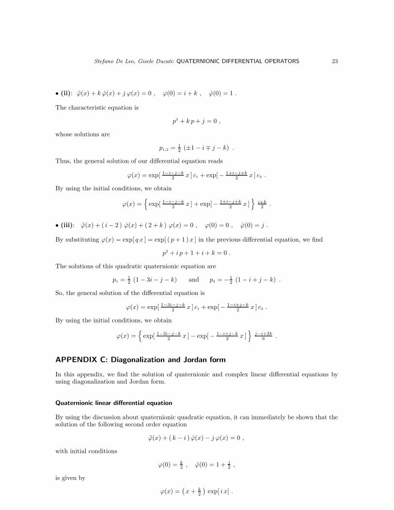
• (ii): ϕ(x) + k ϕ(x) + j ϕ(x) = 0 , ϕ(0) = i + k , ϕ(0) = 1 .

The characteristic equation is

p2 + k p + j = 0 ,

whose solutions are

p1,2 = 1

2(±1 − i ∓ j − k) .

Thus, the general solution of our differential equation reads

ϕ(x) = exp[ 1−i−j−k2

x ] c1 + exp[− 1+i−j+k2

x ] c2 .

By using the initial conditions, we obtain

ϕ(x) ={

exp[ 1−i−j−k

2x ] + exp[− 1+i−j+k

2x ]}

i+k2

.

• (iii): ϕ(x) + ( i − 2 ) ϕ(x) + ( 2 + k ) ϕ(x) = 0 , ϕ(0) = 0 , ϕ(0) = j .

By substituting ϕ(x) = exp[ q x ] = exp[ ( p + 1 )x ] in the previous differential equation, we find

p2 + i p + 1 + i + k = 0 .

The solutions of this quadratic quaternionic equation are

p1 = 1

2(1 − 3i − j − k) and p2 = − 1

2(1 − i + j − k) .

So, the general solution of the differential equation is

ϕ(x) = exp[ 1−3i−j−k

2x ] c1 + exp[− 1−i+j−k

2x ] c2 .

By using the initial conditions, we obtain

ϕ(x) ={

exp[ 1−3i−j−k2

x ] − exp[− 1−i+j−k2

x ]}

j−i+2k6

.

APPENDIX C: Diagonalization and Jordan form

In this appendix, we find the solution of quaternionic and complex linear differential equations byusing diagonalization and Jordan form.

Quaternionic linear differential equation

By using the discussion about quaternionic quadratic equation, it can immediately be shown that thesolution of the following second order equation

ϕ(x) + ( k − i ) ϕ(x) − j ϕ(x) = 0 ,

with initial conditions

ϕ(0) = k2

, ϕ(0) = 1 + j2

,

is given by

ϕ(x) =(

x + k2

)

exp[ i x] .

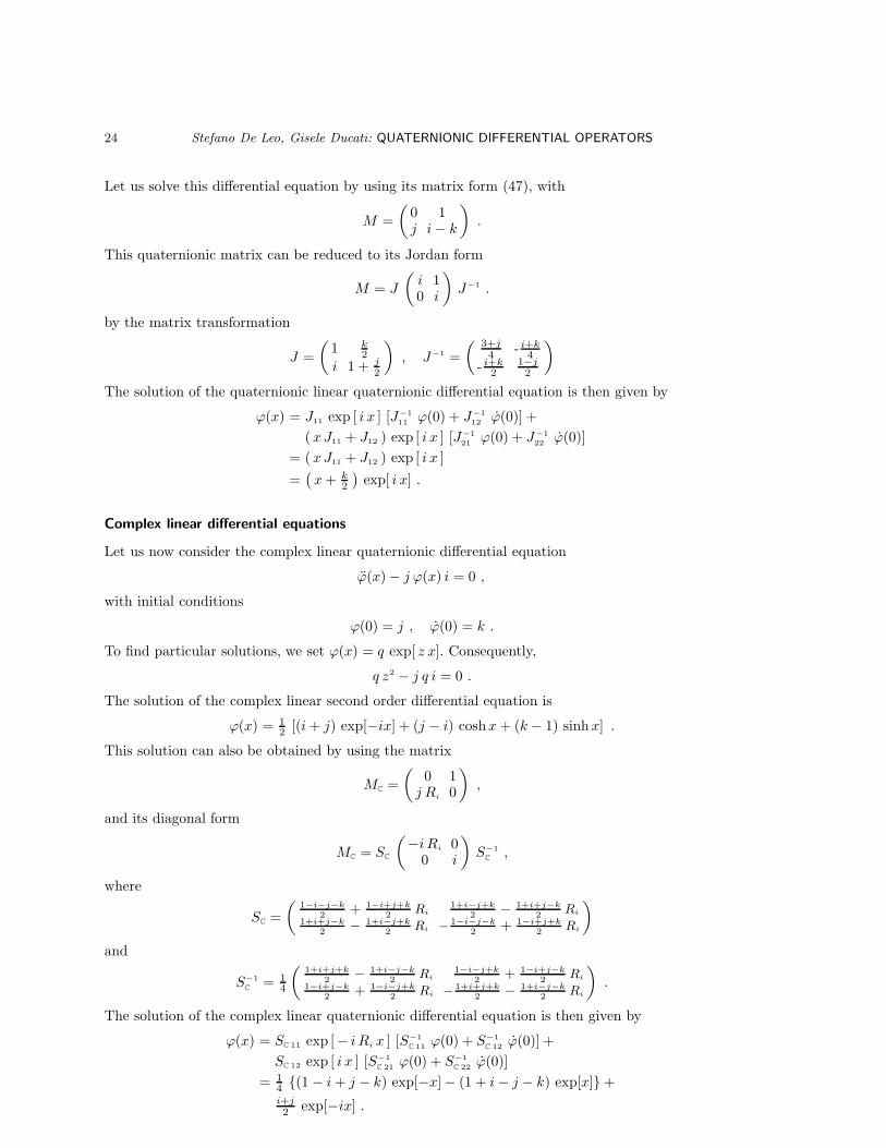
24 Stefano De Leo, Gisele Ducati: QUATERNIONIC DIFFERENTIAL OPERATORS

Let us solve this differential equation by using its matrix form (47), with

M =

(

0 1j i − k

)

.

This quaternionic matrix can be reduced to its Jordan form

M = J

(

i 10 i

)

J−1 .

by the matrix transformation

J =

(

1 k2

i 1 + j

2

)

, J−1 =

(

3+j

4- i+k

4

- i+k2

1−j2

)

The solution of the quaternionic linear quaternionic differential equation is then given by

ϕ(x) = J11 exp [ i x ] [J−1

11ϕ(0) + J−1

12ϕ(0)] +

(xJ11 + J12 ) exp [ i x ] [J−1

21ϕ(0) + J−1

22ϕ(0)]

= (xJ11 + J12 ) exp [ i x ]

=(

x + k2

)

exp[ i x] .

Complex linear differential equations

Let us now consider the complex linear quaternionic differential equation

ϕ(x) − j ϕ(x) i = 0 ,

with initial conditions

ϕ(0) = j , ϕ(0) = k .

To find particular solutions, we set ϕ(x) = q exp[ z x]. Consequently,

q z2 − j q i = 0 .

The solution of the complex linear second order differential equation is

ϕ(x) = 1

2[(i + j) exp[−ix] + (j − i) coshx + (k − 1) sinhx] .

This solution can also be obtained by using the matrix

MC =

(

0 1j Ri 0

)

,

and its diagonal form

MC = SC

(

−i Ri 00 i

)

S−1

C,

where

SC =

(

1−i−j−k

2+ 1−i+j+k

2Ri

1+i−j+k

2− 1+i+j−k

2Ri

1+i+j−k

2− 1+i−j+k

2Ri − 1−i−j−k

2+ 1−i+j+k

2Ri

)

and

S−1

C= 1

4

(

1+i+j+k

2− 1+i−j−k

2Ri

1−i−j+k

2+ 1−i+j−k

2Ri

1−i+j−k

2+ 1−i−j+k

2Ri − 1+i+j+k

2− 1+i−j−k

2Ri

)

.

The solution of the complex linear quaternionic differential equation is then given by

ϕ(x) = SC 11 exp [− i Ri x ] [S−1

C 11ϕ(0) + S−1

C 12ϕ(0)] +

SC 12 exp [ i x ] [S−1

C 21ϕ(0) + S−1

C 22ϕ(0)]

= 1

4{(1 − i + j − k) exp[−x] − (1 + i − j − k) exp[x]} +

i+j

2exp[−ix] .

Stefano De Leo, Gisele Ducati: QUATERNIONIC DIFFERENTIAL OPERATORS 25

References

1. D. Finkelstein, J. M. Jauch, S. Schiminovich and D. Speiser, “Foundations of quaternion quantum me-chanics”, J. Math. Phys. 3, 207–220 (1992).

2. D. Finkelstein and J. M. Jauch and D. Speiser, “Principle of general q covariance”, J. Math. Phys. 4,788–796 (1963).

3. D. Finkelstein and J. M. Jauch and D. Speiser, “Quaternionic representations of compact groups”, J.Math. Phys. 4, 136–140 (1963).

4. S. L. Adler, “Scattering and decay theory for quaternionic quantum mechanics and the structure ofinduced T non-conservation”, Phys. Rev. D 37, 3654–3662 (1998).

5. A. J. Davies, “Quaternionic Dirac equation”, Phys. Rev. D 41, 2628–2630 (1990).6. S. De Leo and P. Rotelli, “Quaternion scalar field”, Phys. Rev. D 45, 575–579 (1992).7. S. L. Adler, “Composite leptons and quark constructed as triply occupied quasi-particle in quaternionic

quantum mechanics”, Phys. Lett. 332B, 358–365 (1994).8. S. L. Adler, “Algebraic and geometric aspects of generalized quantum dynamics”, Phys. Rev. D 49,

6705–6708 (1994).9. S. De Leo and P. Rotelli, “Quaternion Higgs and the electroweak gauge group”, Int. J. Mod. Phys. A 10,

4359–4370 (1995).10. S. De Leo and P. Rotelli, “The quaternionic Dirac lagrangian”, Mod. Phys. Lett. A 11, 357–366 (1996).11. S. De Leo and P. Rotelli, “Quaternionic electroweak theory”, J. Phys. G 22, 1137–1150 (1996).12. S. L. Adler, “Generalized quantum dynamics as pre-quantum mechanics”, Nucl. Phys. B473, 199–244

(1996).13. S. De Leo and W. A. Rodrigues Jr, “Quaternionic electron theory: Dirac’s equation”, Int. J. Theor. Phys.

37, 1511–1529 (1998).14. S. De Leo and W. A. Rodrigues Jr, “Quaternionic electron theory: geometry, algebra and Dirac’s spinors”,

Int. J. Theor. Phys. 37, 1707–1720 (1998).15. A. J. Davies and B. H. McKellar, “Non-relativistic quaternionic quantum mechanics”, Phys. Rev. A 40,

4209–4214 (1989).16. A. J. Davies and B. H. McKellar, “Observability of quaternionic quantum mechanics”, Phys. Rev. A 46,

3671–3675 (1992).17. S. De Leo and P. Rotelli, “Representations of U(1, q) and constructive quaternion tensor product”, Nuovo

Cimento B 110, 33–51 (1995).18. G. Scolarici and L. Solombrino, “Notes on quaternionic groups representation”, Int. J. Theor. Phys. 34,

2491–2500 (1995).19. S. L. Adler, “Projective group representations in quaternionic Hilbert space”, J. Math. Phys. 37, 2352–

2360 (1996).20. S. De Leo, “Quaternions for GUTs”, Int. J. Theor. Phys. 35, 1821–1837 (1996).21. S. De Leo, “Quaternions and special relativity”, J. Math. Phys. 37, 2955–2968 (1996).22. F. Zhang, “Quaternions and matrices of quaternions”, Lin. Alg. Appl. 251, 21–57 (1997).23. G. Scolarici and L. Solombrino, “Quaternionic representation of magnetic groups”, J. Math. Phys. 38,

1147–1160 (1997).24. S. L. Adler and G. G. Emch, “A rejoinder on quaternionic projective representations”, J. Math. Phys.

38, 4758–4762 (1997).25. T. Dray and C. Manogue, “The octonionic eigenvalue problem”, Adv. Appl. Cliff. Alg. 8, 341–364 (1998).26. T. Dray and C. Manogue, “Finding octonionic eigenvectors using mathematica”, Comput. Phys. Comm.

115, 536–547 (1998).27. T. Dray and C. Manogue, “Dimensional reduction”, Mod. Phys. Lett. A 14, 99–104 (1999).28. T. Dray and C. Manogue, “The exponential Jordan eigenvalue problem”, Int. J. Theor. Phys. 38, 2901–

2916 (1999).29. S. De Leo and G. C. Ducati, “Quaternionic groups in physics”, Int. J. Theor. Phys. 38, 2197–2220 (1999).30. A. Baker, “Right eigenvalues for quaternionic matrices: a topological approach”, Lin. Alg. Appl. 286,

303–309 (1999).31. S. De Leo and G. Scolarici, “Right eigenvalue equation in quaternionic quantum mechanics”, J. Phys. A

33, 2971–2995 (2000).32. L. P. Horwitz and L. C. Biedenharn, “Quaternion quantum mechanics: second quantization and gauge

field”, Ann. Phys. 157, 432–488 (1984).33. S. L. Adler, “Generalized quantum dynamics”, Nucl. Phys. B415, 195–243 (1994).34. S. De Leo and W. A. Rodrigues Jr, “Quaternionic quantum mechanics: from complex to complexified

quaternions”, Int. J. Theor. Phys. 36, 2725–2757 (1997).35. G. M. Dixon, Division algebras: octonions, quaternions, complex numbers and the algebraic design of

physics (Boston: Kluwer Academic Publushers, 1994).

26 Stefano De Leo, Gisele Ducati: QUATERNIONIC DIFFERENTIAL OPERATORS

36. S. L. Adler, Quaternionic quantum mechanics and quantum fields, (New York: Oxford University Press,1995).

37. F. Gursey and C. H. Tze, On the role of division, Jordan and related algebras in particle physics, (Singa-pore: World Scientific, 1996).

38. I. Niven, “Equations in quaternions”, Amer. Math. Monthly 48, 654–661 (1941).39. I. Niven, “The roots of a quaternion”, Amer. Math. Monthly 49, 386–388 (1942).40. L. Brand, “The roots of a quaternion”, Amer. Math. Monthly 49, 519–520 (1942).41. S. Eilenberg and I. Niven, “The fundamental theorem of algebra for quaternions”, Bull. Amer. Math. Soc.

52, 246–248 (1944).42. S. De Leo and P. Rotelli, “Translations between quaternion and complex quantum mechanics”, Prog.

Theor. Phys. 92, 917–926 (1994).43. S. De Leo and P. Rotelli, “Odd dimensional translation between complex and quaternionic quantum

mechanics”, Prog. Theor. Phys. 96, 247–255 (1996).44. P. Rotelli, “The Dirac equation on the quaternionic field”, Mod. Phys. Lett. A 4, 993–940 (1989).45. J. Rembielinski, “Tensor product of the octonionic Hilbert spaces and colour confinement”, J. Phys. A

11, 2323–2331 (1978).46. J. L. Brenner, “Matrices of quaternions”, Pacific J. Math. 1, 329–335 (1951).47. J. L. Brenner, “Applications of the Dieudonne determinant”, Lin. Alg. Appl. 1, 511–536 (1968).48. F. J. Dyson, “Quaternionion determinant”, Helv. Phys. Acta 45, 289–302 (1972).49. L. X. Chen, “Inverse matrix and properties of double determinant over quaternionic field”, Science in

China 34, 528–540 (1991).50. N. Cohen and S. De Leo, “The quaternionic determinant”, Elec. J. Lin. Alg. 7, 100–111 (2000).51. E. Study, “Zur Theorie der linearen gleichungen”, Acta Math. 42, 1–61 (1920).52. J. Dieudonne, “Les determinants sur un corp non-commutatif”, Bull. Soc. Math. France 71, 27–45 (1943).53. H. Aslaksen, “Quaternionic determinants”, Math. Intel. 18, 57–65 (1996).