Symmetries of Modules of Differential Operators

arX

iv:m

ath-

ph/0

5060

44v1

16

Jun

2005

Symmetries of modules of differential operators

H. Gargoubi ‡ P. Mathonet § V. Ovsienko ¶

Abstract

Let Fλ(S1) be the space of tensor densities of degree (or weight) λ on the circle S1. The space Dkλ,µ(S1)

of k-th order linear differential operators from Fλ(S1) to Fµ(S1) is a natural module over Diff(S1), the

diffeomorphism group of S1. We determine the algebra of symmetries of the modules Dkλ,µ(S1), i.e., the

linear maps on Dkλ,µ(S1) commuting with the Diff(S1)-action. We also solve the same problem in the

case of straight line R (instead of S1) and compare the results in the compact and non-compact cases.

1 Introduction

We study the space of linear differential operators acting in the space of tensor densities on S1

as a module over the group Diff(S1) of all diffeomorphisms of S1. More precisely, let Dkλ,µ(S1)

be the space of linear k-th order differential operators

A : Fλ(S1) → Fµ(S1)

where Fλ(S1) and Fµ(S1) are the spaces of tensor densities of degree λ and µ respectively. Wecompute the commutant of the Diff(S1)-action on Dk

λ,µ(S1). This commutant is an associative

algebra which we denote Ikλ,µ(S1) and call the algebra of symmetries.

1.1 This paper is closely related to the classical subject initiated by Veblen [30] in his talkat IMC in 1928, namely the study of invariant operators also called natural operators (cf. [16]).An operator is called invariant if it commutes with the action of the group of diffeomorphisms.The main two examples are the classic de Rham differential of differential forms

d : Ωk(M) → Ωk+1(M),

where M is a smooth manifold, and the integral∫

: Ωn(M) → R

provided M is compact of dimension n.Usually, one considers differential operators acting on various spaces of tensor fields on a

smooth manifold. A famous theorem states that the de Rham differential is, actually, theonly invariant differential operator in one argument acting on the spaces of tensor fields. Thisresult was conjectured by Schouten and proved independently and using different approaches byRudakov [27], Kirillov [14] and Terng [29], for a complete historical account see [12].

‡I.P.E.I.M., Route de Kairouan, 5019 Monastir Tunisie, [email protected],§Institut de Mathematique, Grand traverse 12, B37, 4000 Liege, Belgique, [email protected],¶CNRS, Institut Camille Jordan Universite Claude Bernard Lyon 1, 21 Avenue Claude Bernard, 69622 Villeur-

banne Cedex, FRANCE; [email protected]

Many classification results are available now, and it was shown that there are quite fewinvariant differential operators and most of them are of a great importance. For instance,bilinear invariant differential operators on tensor fields were classified by Grozman [11]. Thecomplete list of such operators contains well-known examples, such as the Poisson, Schoutenand Nijenhuis brackets, and one exceptional bilinear third-order differential operator

G : F− 2

3

(S1) ⊗F− 2

3

(S1) → F 5

3

(S1). (1.1)

Note that differential operators invariant with respect of the diffeomorphism groups can beinterpreted in terms of the Lie algebras of vector fields. This viewpoint relates the subject withthe Gelfand-Fuchs cohomology, see [7] and references therein.

1.2 The main difference of our work from the classic literature is that we consider linearoperators acting on differential operators (instead of tensor fields). More precisely, we classifythe linear maps

T : Dkλ,µ(S1) → Dk

λ,µ(S1) (1.2)

commuting with the Diff(S1)-action. The module of differential operators Dkλ,µ(S1) is not iso-

morphic to any module of tensor fields (but rather rasembles gl(Fλ) or F∗λ ⊗Fµ). The problem

of classification of Diff(S1)-invariant operators on Dkλ,µ(S1) is, therefore, different from Veblen’s

problem, although similar.A well-known example of a map (1.2) is the conjugation of differential operators. This map

associates to an operator A the adjoint operator A∗. If A ∈ Dkλ,µ(S1), then A∗ ∈ Dk

1−µ,1−λ(S1),so that this map defines a symmetry if and only if λ+ µ = 1.

Let us emphasize that, unlike Rudakov-Kirillov-Terng, we consider not only differential (orlocal) symmetries of Dk

λ,µ(S1) but also non-local ones. For instance, we find a version of tracewhich is an analog of the Adler trace (see [1]).

1.3 The main purpose of this paper is to show that some modules Dkλ,µ(S1) are particular

and very interesting. It turns out that the algebra of symmetries Ikλ,µ(S1) can be quite rich

depending on the values of λ and µ as well as on k. This algebra is an important characteristicof the corresponding module which embraces those given in [9, 8, 10].

The first example which is particular (for every k) is the module Dk0,1(S

1) of operators fromthe space of functions to the space of 1-forms. The algebra of symmetries in this case is alwaysof maximal dimension.

Another interesting module is D2− 1

2, 32

(S1). It is related to the famous Virasoro algebra and

also to the projective differential geometry, see [13, 25]. This module appears as a particularcase in our classification.

Further intriguing examples of modules of differential operators are D3− 2

3, 53

(S1) and D4− 2

3, 53

(S1).

These modules are related to the Grozman operator (1.1). The algebraic and geometric meaningof these modules is not known.

1.4 We will also consider symmetries of differential operators acting in the space of λ-densitiesover R and compare this case with the case of S1. The classification of the invariant differentialoperators (1.2) remains the same as that on S1, except that there are no non-local symmetries.

Let us also mention that symmetries of the modules of differential operators in the multi-dimensional case have been classified in [22]. In this case the algebra of symmetries is smaller.

1.5 This paper is organized as follows. In Section 2 we introduce the Diff(S1)-modules ofdifferential operators and their symbols. In Section 3 we formulate the classification theorems. In

2

Section 4 we give an explicit construction of all Diff(S1)-invariant linear maps on the modulesDk

λ,µ(S1) in all possible cases. These operators are our main characters; some of them areknown and some seem to be new. In Section 5 we calculate the associative algebras of invariantoperators and identify them with some associative algebras of matrices. This gives a completedescription of the symmetry algebras Ik

λ,µ(S1). Finally, in Section 6 we prove that there are

no other invariant operators on Dkλ,µ(S1) than the operators we introduce. This completes the

proof of the main theorems.

2 The main definitions

In this section we define the space of differential operators on S1 acting on the space of densitiesand the corresponding space of symbols. We pay particular attention to the action of the groupof diffeomorphisms Diff(S1) and of the Lie algebra of vector fields Vect(S1) on these spaces.

2.1 Densities on S1

Denote by Fλ(S1), or Fλ for short, the space of λ-densities on S1

ϕ = φ(x)(dx)λ,

where λ ∈ C is the degree (or weight), x is a local coordinate on S1 and φ(x) ∈ C∞(S1). As avector space, Fλ is isomorphic to C∞(S1).

The group Diff(S1) naturally acts on Fλ. If f ∈ Diff(S1), then

ρλf−1 : φ(x)(dx)λ 7→

(

f ′)λφ(f(x))(dx)λ .

The Diff(S1)-modules Fλ and Fµ are not isomorphic unless λ = µ (cf. [7]).

Example 2.1. The space F0 is isomorphic to C∞(S1), as a Diff(S1)-module; the space F1 isnothing but the space of 1-forms (volume forms); the space F−1 is the space of vector fields onS1.

The space Fλ can also be viewed as the space of functions on the cotangent bundle T ∗S1 \S1

(with zero-section removed) homogeneous of degree −λ. In standard (Darboux) coordinates(x, ξ) on T ∗S1 one writes:

φ(x)(dx)λ ↔ φ(x) ξ−λ. (2.1)

This identification commutes with the Diff(S1)-action.

2.2 Invariant pairing

There is a pairing Fλ ⊗F1−λ → R given by

⟨

φ(x)(dx)λ, ψ(x)(dx)1−λ⟩

=

∫

S1

φ(x)ψ(x)dx

which is Diff(S1)-invariant. For instance, the space F 1

2

is equipped with a scalar product; this

is a natural pre-Hilbert space that is popular in geometric quantizaton.

3

2.3 Differential operators on densities

Consider the space of linear differential operators

A : Fλ → Fµ

with arbitrary λ, µ ∈ C. This space will be denoted by Dλ,µ(S1). The subspace of differentialoperators of order ≤ k will be denoted by Dk

λ,µ(S1).

Fix a (local) coordinate x, a differential operator A ∈ Dkλ,µ(S1) is of the form

A = ak(x)dk

dxk+ ak−1(x)

dk−1

dxk−1+ · · · + a0(x), (2.2)

where ai(x) are smooth functions. More precisely,

A(ϕ) =

(

ak(x)dkφ(x)

dxk+ ak−1(x)

dk−1φ(x)

dxk−1+ · · · + a0(x)φ(x)

)

(dx)µ,

where ϕ = φ(x)(dx)λ.

Example 2.2. The space D0λ,µ(S1) is nothing but Fµ−λ. Any zeroth-order differential operator

is the operator of multiplication by a (µ− λ)-density:

a(x)(dx)µ−λ : φ(x)(dx)λ 7→ a(x)φ(x)(dx)µ

2.4 Diff(S1)- and Vect(S1)-module structure

The space Dλ,µ(S1) is a Diff(S1)-module with respect to the action

ρλ,µf (A) = ρµ

f A ρλf−1 ,

where f ∈ Diff(S1).We will also consider the Lie algebra of vector fields Vect(S1) and the natural Vect(S1)-

action on Dkλ,µ(S1). A vector field X = X(x) d

dxacts on the space of tensor densities Fλ by Lie

derivativeLλ

X(ϕ) =(

X(x)φ′(x) + λX ′(x)φ(x))

(dx)λ.

The action of Vect(S1) on the space of differential operators is given by the commutator

Lλ,µX (A) = Lµ

X A−A LλX . (2.3)

Note that the above formulæ are independent of the choice of the local coordinate x.

2.4.1 Example: the module D1λ,µ(S1)

The space D1λ,µ(S1) is split into a direct sum

D1λ,µ(S1) ∼= Fµ−λ−1 ⊕Fµ−λ (2.4)

as a Diff(S1)- (and Vect(S1)-) module.Indeed, every first-order differential operator A ∈ D1

λ,µ(S1)

A(

φ(x)(dx)λ)

=(

a1(x)φ′(x) + a0(x)φ(x)

)

(dx)µ

4

can be rewritten in the form

A(

φ(dx)λ)

=(

a1 φ′ + λa′1 φ+ (a0 − λa′1)φ

)

(dx)µ,

and, finally, one obtaines an intrinsic expression

A(ϕ) =(

La1ϕ+ (a0 − λa′1)ϕ

)

(dx)µ−λ,

where a1 = a1(x)ddx

is understood a vector field and a0(x) − λa′1(x) as a function.Furthermore, using identification (2.1), one can write a more elegant formula for a first-order

operator:

A = ξµ−λ La1+ diva1

∂

∂ξ+ a0.

Note that there are no intrinsic formulæ similar to the above ones in the case of modulesDk

λ,µ(S1) with k ≥ 2, and, in general, there are no splittings similar to (2.4). The geometric

meaning of the modules Dkλ,µ(S1) was discussed in [9, 2, 8, 10].

2.5 Space of symbols of differential operators

The filtrationD0

λ,µ(S1) ⊂ D1λ,µ(S1) ⊂ · · · ⊂ Dk

λ,µ(S1) ⊂ · · ·is preserved by the Diff(S1)-action. The graded Diff(S1)-module Sλ,µ(S1) = gr (Dλ,µ(S1)) iscalled the module of symbols of differential operators.

The quotient module Dkλ,µ(S1)/Dk−1

λ,µ (S1) is isomorphic to the module of tensor densities

Fµ−λ−k(S1); the isomorphism is provided by the principal symbol. As a Diff(S1)-module, the

space of symbols depends, therefore, only on the difference

δ = µ− λ,

so that Sλ,µ(S1) can be denoted as Sδ(S1), and finally we have

Sδ(S1) =

∞⊕

i=0

Fδ−i

as Diff(S1)-modules.The space of symbols Sδ(S

1) can also be viewed as the space of functions on T ∗S1 \ S1.Namely, any k-th order symbol P ∈ Sδ(S

1) can be written in the form

P = ak(x) ξk−δ + ak−1(x) ξ

k−δ−1 + · · · + a0(x) ξ−δ . (2.5)

The natural lift of the action of Diff(S1) to T ∗S1 equips the space of functions (2.5) with astructure of Diff(S1)-module; this action coincides with the Diff(S1)-action on the space Sδ(S

1).

Remark 2.3. The spaces Dλ,µ(S1) and Sδ(S1) are not isomorphic as Diff(S1)-modules. There

are cohomology classes which are obstructions for existence of such an isomorphism, see [20, 2, 9].

3 The main results

In this section we formulate the main results of this paper and give a complete description ofthe algebras of symmetries Ik

λ,µ(S1). We defer the proofs to Sections 4-6.

We will say that the algebra Ikλ,µ(S1) is trivial if it is generated by the identity map Id,

and therefore is isomorphic to R. Of course, we are interested in the cases when this algebra isnon-trivial.

5

3.1 Introducing four algebras of matrices

We will need the following associative algebras.

1. The commutative algebra R ⊕ · · · ⊕ R will be denoted by Rn. Of course, this algebra can

be represented by diagonal n× n-matrices.

2. The algebra of (lower) triangular (n×n)-matrices will be denoted by tn.

3. The commutative algebra a of (2 ×2)-matrices of the form

(

a 0b a

)

.

4. The algebra b of (4 ×4)-matrices of the form

a 0 0 d0 a 0 00 c b 00 0 0 b

It turns out that the algebras of symmetries Ikλ,µ(S1) are always direct sums of the above

matrix algebras.In Appendix we will introduce natural generators of the algebras a, b and R

n.

3.2 Stability: the case k ≥ 5

We start our list of classification theorems with the “stable” case. Namely, if k ≥ 5, then thealgebras Ik

λ,µ(S1) do not depend on k.

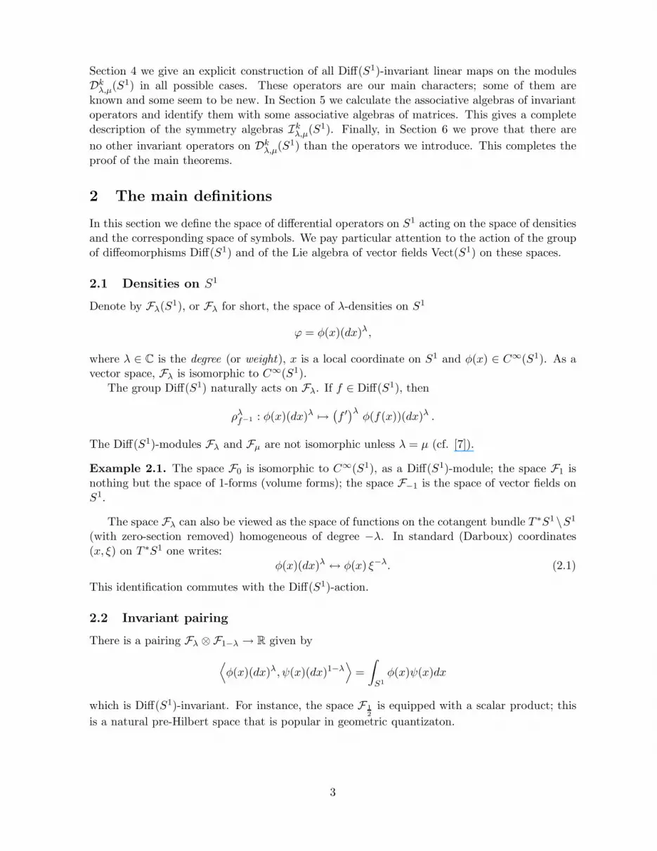
Theorem 3.1. For k ≥ 5, the algebra Ikλ,µ(S1) is trivial for all (λ, µ), except

1. Ikλ,µ(S1) ∼= R

2, for

λ+ µ = 1, λ 6= 0,λ = 0, µ 6= 1, 0µ = 1, λ 6= 1, 0

2. Ik0,0(S

1) ∼= Ik1,1(S

1) ∼= R3;

3. Ik0,1(S

1) ∼= b ⊕ R2.

The exceptional modules Dkλ,µ(S1) with k ≥ 5 are represented in Figure 1.

We will provide in the sequel a list of generators of the symmetry algebra for each non-trivialcase, we will also give its explicit identification with the corresponding algebra of matrices.

3.3 Modules of differential operators of order 4

The result for the modules Dkλ,µ(S1) with k ≤ 4 is different from the above one. (It is interesting

to compare this property of differential operators with that in the case of algebraic equations.)Consider the modules of operators of order k = 4. The complete classification of symmetries

in this case is given by the following result.

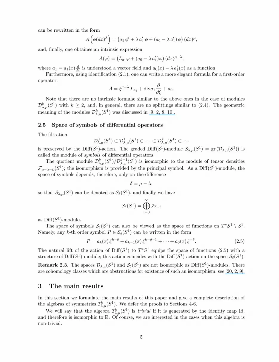
Theorem 3.2. The algebra I4λ,µ(S1) is trivial for all (λ, µ) except

6

µ

λ

(0,0)

(0,1) (1,1)

Figure 1: Exceptional modules of higher order operators

1. I4λ,µ(S1) ∼= R

2, for

λ+ µ = 1, λ 6= 0, −23

λ = 0, µ 6= 3, 54 , 1, 0

µ = 1, λ 6= 1, 0, −14 , −2

2. I4λ,µ(S1) ∼= R

3, for (λ, µ) = (1, 1), (0, 54 ), (0, 0), (−1

4 , 1), (−23 ,

53);

3. I40,3(S

1) ∼= I4−2,1(S

1) ∼= a ⊕ R;

4. I40,1(S

1) ∼= b ⊕ R2.

The exceptional modules D4λ,µ(S1) are represented in Figure 2.

µ

λ

(0,0)

(1,1)(-2,1)

(0,3)

(0, )2

_4

( ,1)1_4

-

5( , )-3 3

5__

Figure 2: Exceptional modules of 4-th order operators

Remark 3.3. We will show in Section 5.4.1 that the module D4− 2

3, 53

(S1) is, indeed, a very special

one. This exceptional module is related to the Grozman operator (1.1).

3.4 Modules of differential operators of order 3

Symmetries of the modules of third-order operators are particularly rich.

Theorem 3.4. The algebra I3λ,µ(S1) is trivial for all (λ, µ) except

7

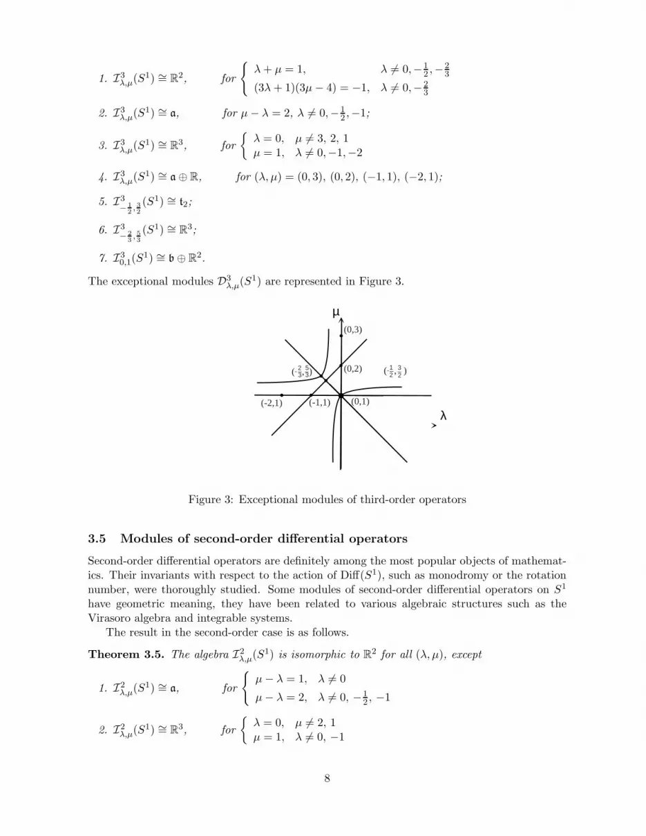
1. I3λ,µ(S1) ∼= R

2, for

λ+ µ = 1, λ 6= 0,−12 ,−2

3

(3λ+ 1)(3µ− 4) = −1, λ 6= 0,−23

2. I3λ,µ(S1) ∼= a, for µ− λ = 2, λ 6= 0,−1

2 ,−1;

3. I3λ,µ(S1) ∼= R

3, for

λ = 0, µ 6= 3, 2, 1µ = 1, λ 6= 0,−1,−2

4. I3λ,µ(S1) ∼= a ⊕ R, for (λ, µ) = (0, 3), (0, 2), (−1, 1), (−2, 1);

5. I3− 1

2, 32

(S1) ∼= t2;

6. I3− 2

3, 53

(S1) ∼= R3;

7. I30,1(S

1) ∼= b ⊕ R2.

The exceptional modules D3λ,µ(S1) are represented in Figure 3.

µ

λ

2( , )-3 3

5__

(-2,1)

(0,3)

(-1,1)

(0,2)

(0,1)

( , )1_2

- 3_2

Figure 3: Exceptional modules of third-order operators

3.5 Modules of second-order differential operators

Second-order differential operators are definitely among the most popular objects of mathemat-ics. Their invariants with respect to the action of Diff(S1), such as monodromy or the rotationnumber, were thoroughly studied. Some modules of second-order differential operators on S1

have geometric meaning, they have been related to various algebraic structures such as theVirasoro algebra and integrable systems.

The result in the second-order case is as follows.

Theorem 3.5. The algebra I2λ,µ(S1) is isomorphic to R

2 for all (λ, µ), except

1. I2λ,µ(S1) ∼= a, for

µ− λ = 1, λ 6= 0

µ− λ = 2, λ 6= 0, −12 , −1

2. I2λ,µ(S1) ∼= R

3, for

λ = 0, µ 6= 2, 1µ = 1, λ 6= 0, −1

8

3. I2− 1

2, 32

(S1) ∼= t2;

4. I20,2(S

1) ∼= I2−1,1(S

1) ∼= a ⊕ R;

5. I20,1(S

1) ∼= b ⊕ R.

The exceptional modules of second-order operators are represented in Figure 4.

µ

λ

( , )1_2

- 3_2

(0,2)

(-1,1) (0,1)

Figure 4: Exceptional modules of second-order operators

3.6 Modules of first-order differential operators

Let us finish this section with the result in the first-order case. The result is less interesting, theonly particular module is D1

0,1(S1).

Theorem 3.6. The algebra of I1λ,µ(S1) is isomorphic to R

2 for all λ, µ, except in the followingcases:

1. I1λ,µ(S1) ∼= a, for µ− λ = 1, λ 6= 0;

2. I10,1(S

1) ∼= b.

For the sake of completeness, let us also mention the zeroth-order case: the algebra ofsymmetries I0

λ,µ(S1) is trivial. Indeed, the module D0λ,µ(S1) is isomorphic to Fµ−λ.

3.7 Non-compact case: differential operators on R

The algebras of symmetries of the modules of differential operators in the spaces of densities overR can be different from that on S1. This occurs in the “most particular” case (λ, µ) = (0, 1).

Theorem 3.7. (i) If (λ, µ) 6= (0, 1), then the algebra Ikλ,µ(R) coincides with Ik

λ,µ(S1).(ii) In the exceptional case (λ, µ) = (0, 1) one has:

1. If k ≥ 3, then Ik0,1(R) ∼= t2 ⊕ R

2;

2. If k = 2, then Ik0,1(R) ∼= t2 ⊕ R;

3. If k = 1, then Ik0,1(R) ∼= t2.

9

4 Construction of symmetries

In this section we give an explicit construction of the generators of algebras Ikλ,µ(S1) for every

case where this algebra is non-trivial. We will prove in Section 6 that our list of invariantdifferential operators is complete.

4.1 The conjugation

The best known invariant map between the spaces of differential operators is the conjugation.It is a linear map

C : Dkλ,µ(S1) → Dk

1−µ,1−λ(S1)

that associates to each operator A its adjoint A∗ defined by

∫

S1

A∗(ϕ)ψ =

∫

S1

ϕA(ψ)

for every ϕ ∈ F1−µ and ψ ∈ Fλ. It follows that the modules Dkλ,µ(S1) with λ and µ satisfying

the conditionλ+ µ = 1

have non-trivial symmetries.The conjugation map C is an involution; the straight line λ + µ = 1 will play a role of

symmetry axis in the plane parameterized by (λ, µ).For an arbitrary local parameter x on S1, the conjugation map is given by the well-known

formula

C :

k∑

i=0

ai(x)di

dxi7→

k∑

i=0

(−1)i(

d

dx

)i

ai(x) (4.1)

that easily follows from the definition.

Remark 4.1. The expression (4.1) is independent from the choice of the parameter x. Indeed,any change of local coordinates is given by a diffeomorphism of S1. Note that this fundamentalproperty of coordinate independence is just a different way to express the Diff(S1)-equivariance.

4.2 The cases λ = 0 and µ = 1

We will define a Diff(S1)-invariant operator

P0 : Dk0,µ(S1) → Dk

0,µ(S1).

Let us first consider a Diff(S1)-invariant projection P0 : Dk0,µ(S1) → Fµ defined by: A 7→ A(1),

where 1 ∈ F0∼= C∞(M) is a constant function on S1. In other words,

P0

(

k∑

i=0

ai(x)di

dxi

)

= a0(x) (dx)µ . (4.2)

Since Fµ ⊂ Dk0,µ(S1), one obtains a non-trivial element of the algebra Ik

0,µ(S1).Thanks to the conjugation map (4.1), one also has a non-trivial symmetry P ∗

0 = C P0 C

P ∗0 : Dk

λ,1(S1) → Dk

λ,1(S1).

10

The explicit formula follows from (4.2) and (4.1):

P ∗0

(

k∑

i=0

ai(x)di

dxi

)

=

k∑

i=0

(−1)i ai(x)(i). (4.3)

The right hand side is understood as a (scalar) differential operator from Fλ to F1.

4.3 Two additional elements of Ik0,1(S

1)

In the most particular case (λ, µ) = (0, 1), there are two more elements of the symmetry algebra.

• There is a non-local element of I10,1(S

1). It is given by the expression

L

(

k∑

i=0

ai(x)di

dxi

)

=

(∫

S1

a0(x) dx

)

d (4.4)

where d is the de Rham differential. Indeed, the projection (4.2) gives a 1-form on S1 sothat the integral above is well-defined; since d ∈ D1

0,1(S1), we can understand L as a linear

map L : Dk0,1(S

1) → Dk0,1(S

1) and therefore a symmetry.

Remark 4.2. Equation (4.4) is an analog of the well-known Adler trace [1], although thelatter is defined on the space of pseudodifferential operators from F0 to F0.

• There is one more element of the algebra I10,1(S

1) given by the formula

P1

(

k∑

i=0

ai(x)di

dxi

)

=

(

k∑

i=1

(−1)i−1 ai(x)(i−1)

)

d. (4.5)

It is easy to check directly that P1 is Diff(S1)-invariant, but its intrinsic form can also bewritten. In the one-dimensional case, the de Rham differential d is an element of D1

0,1(S1).

One has a Diff(S1)-invariant operator

δ : Dk1,µ(S1) → Dk+1

0,µ (S1)

given by right composition with the de Rham differential: δ : A 7→ A d. This map is abijection between Dk

1,µ(S1) and KerP0 ⊂ Dk+10,µ (S1). One has:

P1 = δ P0 C δ−1 (Id − P0).

4.4 Additional elements of Ik0,0(S

1) and Ik1,1(S

1)

The algebra Ik0,0(S

1) is generated by the operator P0 given by (4.2) and

S = −C δ−1 (Id − P0) C δ C. (4.6)

One can check that the explicit formula for this operator is as follows:

S

(

k∑

i=0

ai(x)di

dxi

)

=

k−1∑

i=0

(−1)i(

d

dx

)i

(

ai(x) + a′i+1(x))

+ (−1)k(

d

dx

)k

ak(x).

The algebra Ik1,1(S

1) is generated by P ∗0 given by (4.3) and the operator S∗ = C S C.

11

4.5 Symmetries and bilinear operators on tensor densities

We now give a general way to construct linear Diff(S1)-invariant differential operators onDk

λ,µ(S1). Assume there are two Diff(S1)-invariant differential operators:

• a bilinear differential operator J : Fν ⊗Fλ → Fµ;

• a linear projection π : Dkλ,µ(S1) → Fν .

We define a linear map J π : Dkλ,µ(S1) → Dk

λ,µ(S1) as follows

(J π) (A)(·) = J (π(A), ·) .

This map is obviously Diff(S1)-invariant.This is the way invariant differential operators on the modules Dk

λ,µ(S1) are related to in-variant bilinear differential operators on densities. We give here the complete list of bilinearoperators on densities and the complete list of linear projections. We will then specify thegenerators of the algebras Ik

λ,µ(S1) that can be obtained by the above construction.

4.5.1 Bilinear invariant differential operators on tensor densities

The classification of invariant bilinear differential operators on tensor fields is due to P. Grozman[11]. His list is particularly interesting in the one-dimensional case (see also [6]).

Let us recall here the complete list.

1. Every zeroth-order operator Fν ⊗Fλ → Fν+λ is of the form:

φ(x)(dx)λ ⊗ ψ(x)(dx)µ 7→ c φ(x)ψ(x)(dx)λ+µ,

where c ∈ C. From now on we omit a scalar multiple c.

2. Every first order operator Fν ⊗Fλ → Fν+λ+1 is as follows

φ(x)(dx)ν , ψ(x)(dx)λ

=(

ν φ(x)ψ(x)′ − λφ(x)′ψ(x))

(dx)ν+λ+1, (4.7)

where x is a local coordinate on M and we identify tensor densities with functions. Theoperator (4.7) is nothing but the Poisson bracket on T ∗S1 (or T ∗

R1).

For every (ν, λ) 6= (0, 0), the operator (4.7) is the only Diff(S1)- (or Diff(R1)-) invariantoperator, otherwise there are two linearly independent operators: φd(ψ) and d(φ)ψ, whered is the de Rham differential.

3. There exist second order operators Fν ⊗Fλ → Fν+λ+2 given by the compositions:

φ⊗ ψ 7→ dφ, ψ for ν = 0,

φ⊗ ψ 7→ φ, dψ for λ = 0,

φ⊗ ψ 7→ d φ, ψ for ν + λ = −1.

(4.8)

4. Three third-order bilinear invariant differential operators Fν ⊗Fλ → Fν+λ+3 are also givenby compositions:

φ⊗ ψ 7→ dφ, dψ for (ν, λ) = (0, 0),

φ⊗ ψ 7→ d dφ, ψ for (ν, λ) = (0,−2),

φ⊗ ψ 7→ d φ, dψ for (ν, λ) = (−2, 0).

(4.9)

12

5. The only differential operator of order 3 which is not a composition of the operators oflesser orders is the famous Grozman operator G : F− 2

3

(S1) ⊗ F− 2

3

(S1) → F 5

3

(S1) already

mentioned in Introduction, see (1.1). It is given by the following expression:

G(

φ(x)(dx)−2

3 , ψ(x)(dx)−2

3

)

=

(

2

∣

∣

∣

∣

φ(x) ψ(x)φ′′′(x) ψ′′′(x)

∣

∣

∣

∣

+ 3

∣

∣

∣

∣

φ′(x) ψ′(x)φ′′(x) ψ′′(x)

∣

∣

∣

∣

)

(dx)5

3 . (4.10)

The Diff(S1)-invariance of this operator can be easily checked directly.

Remark 4.3. The operator (4.10) remains one of the most mysterious invariant differentialoperators. Its geometric and algebraic meaning was discussed in [6, 7].

We will use the above bilinear operators to construct the symmetries, but we do not useGrozman’s classification result in our proof.

4.5.2 Invariant projections from Dkλ,µ(S1) to Fν

Let us now give the list of Diff(S1)-invariant linear maps from Dkλ,µ(S1) to the space Fν .

1. The well-known projection is the principal symbol map σ : Dkλ,µ(S1) → Fµ−λ−k. given by

the expression

σ

(

k∑

i=0

ai(x)di

dxi

)

= ak(x) (dx)µ−λ−k . (4.11)

The map σ is obviously Diff(S1)-invariant for all (λ, µ).

2. For all (λ, µ), define a linear map

V : Dkλ,µ(S1) → Fµ−λ−k+1

as follows:V (A) =

(

αa′k(x) + β ak−1(x))

(dx)µ−λ−k+1. (4.12)

where

α = λk +k(k − 1)

2, β = µ− λ− k

It is easy to check that this map is Diff(S1)-invariant. The map (4.12) is a “first-orderanalog” of the principal symbol.

Remark 4.4. If λ + µ = 1, then this map is proportional to the principal symbol of the(k − 1)-th order operator A− (−1)k A∗. In other words,

V = σ (Id − (−1)kC)

if λ+ µ = 1.

3. In the particular case,

λ =1 − k

2, µ =

1 + k

2(4.13)

The map (4.12) vanishes. In this case, there are two independent projections onto F1:

A 7→ a′k(x) dx, A 7→ ak−1(x) dx

which are Diff(S1)-invariant.

13

4. It turns out that for some special values of the parameters λ and µ, there exist second-orderanalogues of the operators (4.11) and (4.12).

Proposition 4.5. For every k ≥ 3 and (λ, µ) satisfying the relation

(

λ+k − 2

3

)(

µ− k + 1

3

)

+1

36(k + 1)(k − 2) = 0, (4.14)

there exists a Diff(S1)-invariant map W : Dkλ, µ → Fµ−λ−k+2 given by

W (A) =(

α2 a′′k(x) + α1 a

′k−1(x) + α0 ak−2(x)

)

(dx)µ−λ−k+2, (4.15)

where the coefficients are defined by

α2 = 23k(k − 1)(k + 3λ− 2)2

α1 = 2(k − 1)(k + 3λ− 2)(2 − 2λ− k)

α0 = 3k2 + 12λk + 12λ2 − 11k − 24λ + 10.

(4.16)

Proof. Straightforward.

5. There exists one more invariant differential projection Dk0,1(S

1) → F0(S1) given by the

compositionπδ = P0 C δ−1 (Id − P0), (4.17)

where P0 is defined by (4.2) and C is the conjugation.

6. If there is an invariant map from Dkλ,µ(S1) to the space of 1-forms F1, then one can integrate

the result and obtain a non-local (i.e., non-differential) invariant linear map with values inR ⊂ F0. For instance, for Dk

0,1(S1), the operator P0 defined by (4.2) satisfies the required

condition. One gets a Diff(S1)-invariant map:

A 7→∫

S1

a0(x) dx, A ∈ Dk0,1(S

1). (4.18)

It was proven in [23] that there are no other Diff(S1)-invariant projections Dkλ,µ(S1) → Fν

than the above ones and their compositions with C and d. We use these operators to constructthe generators of the symmetry algebras (but we do not use the classification result of [23] inthe proofs of our theorems).

5 Computing the algebras of symmetry

We will now investigate, case by case, the non-trivial algebras Ikλ,µ(S1). We will construct the

generators of these algebras and calculate the multiplication tables. We then give an explicitidentification of the algebras Ik

λ,µ(S1) with the matrix algebras introduced in Section 3.1. The

constructions of this section prove that the algebras Ikλ,µ(S1) are at least as big as stated in

Section 3.The proof of the second part of our classification theorems, namely that there are no other

symmetries than we construct and study here, will be given in Section 6.

14

5.1 The algebra Ik0,1(S

1)

Let us start with the most particular algebra Ik0,1(S

1) for all k. One has in this case

Ik0,1(S

1) = Span (Id, C, P0, P∗0 , P1, L)

where the generators are defined by (4.1)-(4.5).Let us now calculate the relations between these generators.

Proposition 5.1. The multiplication table for the associative algebra Ik0,1(S

1) is as follows:

Id P0 C P ∗0 P1 L

Id Id P0 C P ∗0 P1 L

P0 P0 P0 P ∗0 P ∗

0 0 0

C C P0 Id P ∗0 P ∗

0 −P1−P0 −LP ∗

0 P ∗0 P0 P0 P ∗

0 P ∗0 − P0 0

P1 P1 0 −P1 0 P1 L

L L L L L 0 0

(5.1)

Proof. First, consider the product of P1 and C. From the definition (4.1) one obtains

(P1 C)(A) = P1

(

k∑

i=0

(−1)i(

d

dx

)i

ai(x)

)

= P1

k∑

i=0

i∑

j=0

(−1)i(

i

j

)

a(i−j)i (x)

dj

dxj

= P1

k∑

j=0

k∑

i=j

(−1)i(

i

j

)

a(i−j)i (x)

dj

dxj

and then from (4.5) it follows that

=

k∑

j=1

k∑

i=j

(−1)i+j−1

(

i

j

)

a(i−1)i (x)

d

=

k∑

i=1

i∑

j=1

(−1)i+j−1

(

i

j

)

a(i−1)i (x)

d

=

(

k∑

i=1

(−1)i a(i−1)i (x)

)

d

= −P1(A)

as presented in table (5.1).Now, consider the product C P1. One then has from (4.1), (4.5) and (4.3):

(C P1)(A) =

k∑

i=1

(−1)i(

a(i−1)i (x)

d

dx+ a

(i)i (x)

)

= P ∗0 − P1 − P0.

15

Furthermore, one obtains P ∗0 P1 = (P0 C P1)(A) = P ∗

0 − P0.For other products of the the generators the results given in the table immediately follow

from the definition.

Let us finally give an explicit isomorphism between the algebra Ik0,1(S

1) and the matrix

algebra b ⊕ R2 described in Section 3.1.

One checks using the multiplication table (5.1) that the formulæ

a = 12(2P1 + P0 − P ∗

0 ),

b = 12(P0 + P ∗

0 ),

c = 12(P0 − P ∗

0 ),

d = L,

where a, b, c, d are the generators of b, see Appendix 8, define an isomorphism of the associativealgebras

Span(P0, P∗0 , P1, L) ∼= b.

The two more generatorsz1 = Id + C − P0 − P ∗

0

z2 = Id − C − P0 + P ∗0 − 2P1

are in the center and span the second summand R2.

The above generators are linearly independent if k ≥ 3 and span the algebra

Ik0,1(S

1) ∼= b ⊕ R2,

in accordance with Theorem 3.1, 3, Theorem 3.2, 4 and Theorem 3.4, 7.If k = 2, then z2 = 0 so that I2

0,1(S1) ∼= b ⊕ R, see Theorem 3.5, 5. Finally, if k = 1, then

z1 = z2 = 0 and one has I10,1(S

1) ∼= b as stated Theorem 3.6, 2.

5.2 Algebras of symmetry in order k ≥ 5

Assume that k ≥ 5. We already investigated the algebra Ik0,1(S

1). There are two more non-trivial

algebras in this case, namely the algebra Ik0,0(S

1) and the algebra Ik1,1(S

1) which is isomorphic

to Ik0,0(S

1) by conjugation.

The algebra of symmetry Ik0,0(S

1) is as follows

Ik0,0(S

1) = Span (Id, P0, S) ,

where P0 and S are as in (4.2) and (4.6), respectively. These operators are independent fork ≥ 4. We have:

P0 S = S P0 = P0, P 20 = P0, S2 = Id.

Indeed, the first two relations are due to the fact that the scalar term of S(A) is equal to a0(x),cf. eq. (4.6) and the explicit expression for S. Put

1 = Id, a1 = P0 and a2 =1√2(Id − S).

One obtains the generators of the algebra R3, cf. Appendix 8. Finally, one has

Ik0,0(S

1) ∼= R3,

16

as stated in Theorem 3.1, 2.The algebras Ik

0,µ(S1) corresponding to the generic values of µ have only two generators: Id

and P0. These algebras are obviously isomorphic to R2.

5.3 Algebras of symmetry in order 4

Consider the modules of differential operators of order k = 4:

A = a4(x)d4

dx4+ a3(x)

d3

dx3+ a2(x)

d2

dx2+ a1(x)

d

dx+ a0(x).

We will study all the exceptional modules systematically and investigate every non-trivial algebraof symmetry.

The generators of the algebras I40,1(S

1) and I40,0(S

1) ∼= I41,1(S

1) are the same as for k = 5.Let us consider other interesting cases.

5.3.1 The algebras I40, 5

4

(S1) and I4− 1

4,1(S1)

We already constructed two generators of the algebra I40, 5

4

(S1), namely Id and P0. One extra

generator is obtained by the following procedure.The values (λ, µ) = (0, 5

4) satisfy the relation (4.14), so that the map

W : D40, 5

4

(S1) → F− 3

4

defined by (4.15) is Diff(S1)-invariant. There is a second-order bilinear differential operator

J : F− 3

4

⊗F0 → F 5

4

defined by the second formula in (4.8). Applying the construction of Section 4.5 we consider thecomposition J W defined as in Section 4.5 to obtain an element of algebra I4

0, 54

(S1).

Let us now compute the relations between the generators. The constructed map is given bythe following explicit formula

(J W ) (A) =

(

16

7a′′4(x) −

12

7a′3(x) + a2(x)

)

d2

dx2

+4

3

(

12

7a′′′4 (x) − 9

7a′′3(x) +

3

4a′2(x)

)

d

dx.

(5.2)

Note that the right hand side is understood as an element of D40, 5

4

(S1). Since P0(A) = a0(x),

the product of J W and P0 vanishes:

(J W ) P0 = P0 (J W ) = 0.

One also has the relations

P 20 = P0 and (J W )2 = J W.

Finally, one gets the following answer:

I40, 5

4

(S1) = Span (Id, P0, J W ) ∼= R3,

as stated by Theorem 3.2, 2.The conjugation establishes an isomorphism between the algebras I4

− 1

4,1(S1) and I4

0, 54

(S1).

17

5.3.2 The algebras I40,3(S

1) and I4−2,1(S

1)

The algebra I40,3(S

1) has the generators Id, P0 and the following one constructed in Section 4.5.

Consider the projection V : D40,3(S

1) → F0 defined by formula (4.12) and the third-orderbilinear map J : F0 ⊗F0 → F3, namely the first of the three operators (4.9). Their compositionJ V is an element of I4

0,3(S1):

(J V ) (A) =(

6a′′4(x) − a′3(x)) d2

dx2−(

6a′′′4 (x) − a′′3(x)) d

dx, (5.3)

where the right hand side is understood as an element of D40,3(S

1).

Finally, the algebra I40,3(S

1) is of the form

I40,3(S

1) = Span (Id, P0, J V ) .

To obtain the isomorphism I40,3(S

1) ∼= a⊕ R (see Theorem 3.2 part 3), one checks the followingrelations

P0 (J V ) = (J V ) P0 = (J V )2 = 0.

Then the standard generators of a ⊕ R correspond to Id − P0, J V, P0.The algebra I4

−2,1(S1) is isomorphic to I4

0,3(S1) by conjugation.

5.3.3 The algebra I4− 2

3, 53

(S1) and the Grozman operator

The conjugation map C and Id are, of course, generators of symmetry of the module D4− 2

3, 53

(S1).

One extra generator can be obtained as follows.Consider the operator (4.12)

V : D4− 2

3, 53

(S1) → F− 2

3

and compose it with the Grozman operator G given by (4.10); we obtain (up to a constant) thefollowing operator:

(G V ) (A) =(

a3(x) − 2 a′4(x)) d3

dx3+

(

3

2a′3(x) − 3 a′′4(x)

)

d2

dx2

−(

3

2a′′3(x) − 3 a′′′4 (x)

)

d

dx−(

a′′′3 (x) − 2 a(IV )4 (x)

)

(5.4)

which is a generator of I4− 2

3, 53

(S1).

The relations between the conjugation map and the above operator are:

(G V ) C = C (G V ) = −G V.

One also has:(G V )2 = G V.

One easily deduces from the above relations that the algebra

I4− 2

3, 53

(S1) = Span (Id, C,G V )

is, indeed, isomorphic to R3, cf. Theorem 3.2, 2.

18

5.4 Algebras of symmetry in order 3

Consider the differential operators of order k = 3:

A = a3(x)d3

dx3+ a2(x)

d2

dx2+ a1(x)

d

dx+ a0(x).

We will describe all the non-trivial algebras of symmetry.

5.4.1 The algebra I3− 2

3, 53

(S1)

The conjugation map C, as well as the identity Id, are, of course, generators of the symmetryalgebra I3

− 2

3, 53

(S1). Let us construct one more generator. The principal symbol map is of the

form:σ : D3

− 2

3, 53

(S1) → F− 2

3

.

We compose it with the Grozman operator to obtain a new generator G σ. This operatoris given by the same formula (5.4) as above, but with a4(x) ≡ 0. The relations between thegenerators are also the same as above, so that the symmetry algebra is I3

− 2

3, 53

(S1) = R3.

5.4.2 The hyperbola (3λ+ 1)(3µ − 4) = −1

Consider the class of modules D3λ,µ(S1) with (λ, µ) satisfying the quadratic relation

(3λ+ 1)(3µ − 4) = −1, (5.5)

see Theorem 3.4, 1.First of all, we observe that this relation is precisely the relation (4.14) specified for k = 3.

The operator W : D3λ,µ(S1) → Fµ−λ−1 is then well-defined. Composing this operator with the

Poisson bracket (4.7)·, · : Fµ−λ−1 ⊗Fλ → Fµ,

one obtains a generator of the algebra I3λ,µ(S1). Let us denote this generator by W:

W(A) = (µ− λ− 1)(

α2 a′′3(x) + α1 a

′2(x) + α0 a1(x)

) d

dx

−λ(

α2 a′′′3 (x) + α1 a

′′2(x) + α0 a

′1(x)

)

,

(5.6)

where according to (4.16)α2 = (3λ+ 1)2,

α1 = −(3λ+ 1)(1 − 2λ),

α0 = 3λ2 + 3λ+ 1.

In the generic case, (λ, µ) 6= (0, 1) or (−23 ,

53 ) the symmetry algebra has two generators:

I3λ,µ(S1) = Span (Id, S) . The generator W satisfies the relation

W2 = α0(µ− λ− 1)W.

But α0 6= 0 and if µ− λ− 1 = 0, then (5.5) implies (λ, µ) = (0, 1). Finally, in the generic case,one obtains:

I3λ,µ(S1) ∼= R

2.

19

Remark 5.2. The module D3− 2

3, 53

(S1) belongs to the family (5.5). We have already considered

this module separately, see Section 5.4.1. In this case, we have three generators: I3− 2

3, 53

(S1) =

Span (Id, C,W) which are different from G σ. One checks, however, that the generator G σcan be expressed in terms of the above ones:

G σ =1

2(Id − C) − 9

4W.

5.4.3 The line µ− λ = 2

Consider the family of modules D3λ,µ(S1) satisfying the property µ− λ = 2 as in Theorem 3.4,

2.The operator (4.12) is, in this case, V : D3

λ,µ(S1) → F0. Consider its composition with thesecond-order bilinear operator J : F0 ⊗ Fλ → Fµ given by the first formula in (4.8). In thegeneric case, that is, where

(λ, µ) 6= (0, 2) ,(

−12 ,

32

)

, (−1, 1) ,

one has I3λ,µ(S1) = Span (Id, J V ) .

One obtains the following explicit formula for the constructed generator:

(J V ) (A) =(

3(λ+ 1) a′′3(x) − a′2(x)) d

dx− λ

(

3(λ+ 1) a′′′3 (x) − a′′2(x))

(5.7)

and immediately gets the following relation:

(J V )2 = 0.

This implies I3λ,µ(S1) ∼= a in the generic case.

5.4.4 The modules D30,2(S

1), D3−1,1(S

1) and D3− 1

2, 32

(S1)

Let us consider some exceptional modules still satisfying µ− λ = 2.In the case, (λ, µ) = (0, 2), one has an extra generator of symmetry, as compared with the

preceding section. It is given by the operator P0 as in (4.2). One then has from (5.7)

(J V )P0 = 0, P0 (J V ) = 0.

The isomorphismI3

0,2(S1) = Span (Id, J V, P0) ∼= a ⊕ R

is then obvious in accordance with Theorem 3.4, 4.The conjugation map C establishes an isomorphism I3

−1,1(S1) ∼= I3

0,2(S1), so that tha algebra

I3−1,1(S

1) is also isomorphic to a ⊕ R.

In the interesting case D3− 1

2, 32

(S1), the extra generator is given by the conjugation map C,

so that I3− 1

2, 32

(S1) = Span (Id, J V,C) . The relations between the generators are

(J V ) C = J V, C (J V ) = −J V

as follows from (5.7) and (4.1). One obtains

I3− 1

2, 32

(S1) ∼= t2,

as stated by Theorem 3.4, 5.

20

5.4.5 The modules D30,3(S

1) and D3−2,1(S

1)

The principal symbol map (4.11) is as follows σ : D30,3(S

1) → F0. Compose this map with thethird-order bilinear operator J : F0⊗F0 → F3 defined by the first equation in (4.9). The explicitexpression of the constructed generator is

(J σ) (A) = a′3(x)d2

dx2− a′′3(x)

d

dx. (5.8)

The symmetry algebra is then I30,3(S

1) = Span (Id, J σ, P0) . One easily gets the relations

(J σ)P0 = P0 (J σ) = (J σ)2 = 0

and, finally, I30,3(S

1) ∼= a ⊕ R, see Theorem 3.4, 4. The algebra I3−2,1(S

1) is isomorphic to theabove one by conjugation.

5.5 Algebras of symmetry in orders 2

Consider now the modules of differential operators of order 2.For all (λ, µ), there is a generator of the algebra I2

λ,µ(S1) given by the composition of theprojection (4.12)

V : D2λ,µ(S1) → Fµ−λ−1

and the Poisson bracket·, · : Fµ−λ−1 ⊗Fλ → Fµ.

The explicit formula for this generator is as follows:

V(A) = (µ− λ− 1)(

(2λ+ 1) a′2(x) + (µ− λ− 2) a1(x)) d

dx

−λ(

(2λ+ 1) a′′2(x) + (µ− λ− 2) a′1(x))

.

(5.9)

This generator satisfies the following relation:

V2 = (µ− λ− 1)(µ− λ− 2)V.

In the generic case, the algebra of symmetry is I2λ,µ(S1) = Span (Id,V). It is obviously isomorphic

to R2.

If either µ − λ = 1 or µ− λ = 2, then V2 = 0. In these cases, I2λ,µ(S1) = Span (Id,V) ∼= a,

see Theorem 3.5, 1.Of course, if λ = 0, then there is one more generator, namely P0. Then one has

P0 V = V P0 = 0

and so I20,µ(S1) = Span (Id,V, P0) which is isomorphic to R

3 for generic µ while

I20,2(S

1) ∼= I2−1,1(S

1) ∼= a ⊕ R

see Theorem 3.5, 2 and 3.5, 4.In the case where λ + µ = 1, the conjugation map is well-defined. One checks that in this

case the generator (5.9) is a linear combination of Id and C:

V = λ(2λ+ 1) (C − Id)

21

so that I2λ,µ(S1) ∼= R

2.

The exceptional case (λ, µ) = (−12 ,

32) corresponds to (4.13). There are two invariant projec-

tions from D2− 1

2, 32

(S1) to F1 in this case. Composing one of them with the Poisson bracket

·, · : F1 ⊗F− 1

2

→ F 3

2

one obtains a generator

a2(x)d2

dx2+ a1(x)

d

dx+ a0(x) 7→ a′2(x)

d

dx+

1

2a′′2(x)

independent of Id and C. One easily gets an isomorphism I2− 1

2, 32

(S1) ∼= t2.

6 Proof of the main theorems

In this section we prove that there are no other symmetries of the modules Dkλ,µ(S1) than those

constructed above. In other words, we give here a complete classification of symmetries.Let T be a linear map (1.2) commuting with the Diff(S1)-action. There are two cases:

1. The map T is local, that is, one has Supp(T (A)) ⊂ Supp(A) for all A ∈ Dkλ,µ(S1). In this

case, the famous Peetre theorem (see [26]) guarantees that T is a differential operator incoefficients of A.

2. The map T is non-local, that is, for some A ∈ Dkλ,µ(S1) vanishing in an open subset U ⊂ S1,

the operator T (A) does not vanish on U .

These two cases are completely different and should be treated separately.

6.1 The identification

Let us fix a parameter x on S1 and the corresponding coordinate ξ on the fibers of T ∗S1.For our computations, we will need to identify the spaces Dλ,µ(S1) and Sδ(S

1) using themap

σtot : Dλ,µ(S1) → Sδ(S1) (6.1)

assigns to an operator (2.2) the polynomial on T ∗S1 given by (2.5).The map σtot is an isomorphism of vector spaces but not an isomorphism of Diff(S1)-modules.

It will, nevertheless, allow us to compare the Diff(S1)-action on both spaces.

6.2 The affine Lie algebra

We introduce our main tool that will allow un to use the results of the classic invariant theory.Let x be an affine parameter on S1, the Lie algebra aff of affine transformations is the

two-dimensional Lie algebra generated by the translations and linear vector fields:

aff = Span

(

d

dx, x

d

dx

)

. (6.2)

Since aff is a subalgebra of Vect(S1), every Diff(S1)-invariant map has to commute with theaff-action.

22

Proposition 6.1. The aff-action on Dkλ,µ(S1) depends only on the difference µ−λ and coincides

with the action on Sδ(S1) after identification (6.1).

Proof. Straightforward.

The well-known result of invariant theory states that the associative algebra of differentialoperators on T ∗S1 commuting with the aff-action is generated by

E = ξ∂

∂ξand D =

∂

∂x

∂

∂ξ, (6.3)

see [31]. The operator E is called the Euler field and the operator D the divergence.Every differential Diff(M)-invariant operator (1.2) can therefore be expressed in terms of

these operators. In local coordinates, any Diff(M)-invariant map (1.2) is therefore of the form

T = T (E,D).

Example 6.2. The expressionC = exp(D) exp(iπE)

for the conjugation map (4.1) is worth mentioning for the aesthetic reasons.

6.3 The local case: invariant differential operators

We consider the algebra Ikλ,µ

loc(S1) of local (and thus differential) Diff(S1)-invariant linear

maps (1.2).Let us restrict the map T to the homogeneous component Fk−δ in (2.5). Since the Euler

operator E reduces to a constant, one has

T |Fδ−k=

k∑

ℓ=0

Tk,ℓDℓ (6.4)

where Tk,ℓ are some constants.The operator T has to commute with the Vect(S1)-action on Dk

λ,µ(S1). Consider the Lie

subalgebra sl(2) ⊂ Vect(S1) generated by three vector fields:

sl(2) = Span

(

d

dx, x

d

dx, x2 d

dx,

)

. (6.5)

Remark 6.3. Assume that x is an affine parameter on S1, that is, we identify S1 with RP1

with homogeneous coordinates (x1 : x2) and choose x = x1/x2. The vector fields (6.5) are thenglobally defined and correspond to the standard projective structure on RP

1, see, e.g., [13].

Proposition 6.4. A linear map (1.2) written in the form (6.4) is sl(2,R)-invariant if and onlyif it satisfies the recurrence relation

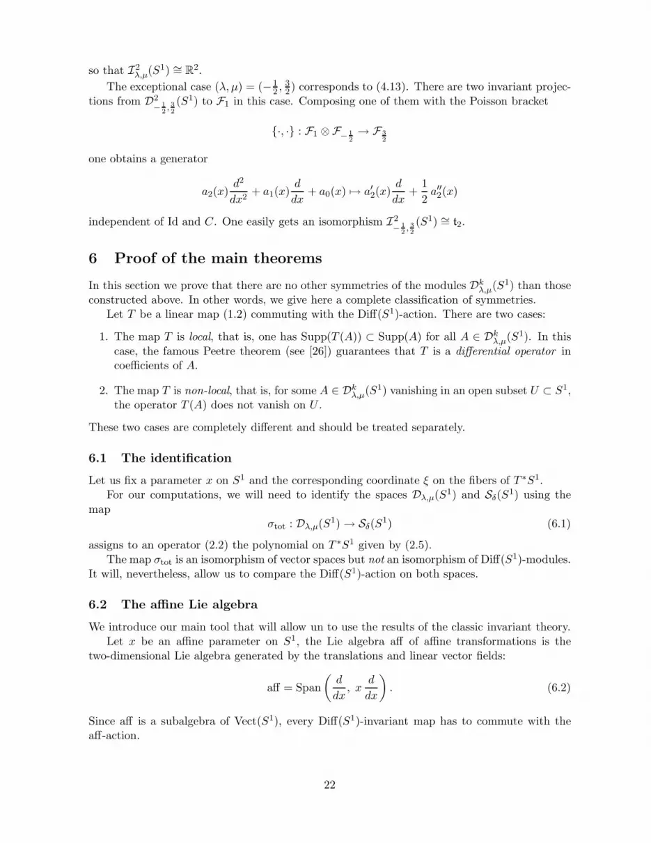
(k + 2λ− 1) Tk−1,ℓ−1 − (k + 2λ− ℓ) Tk,ℓ−1 − ℓ (2(µ− λ) − 2k + ℓ− 1) Tk,ℓ = 0. (6.6)

Proof. The form (6.4) is already invariant with respect to the affine subalgebra (6.2) of sl(2,R).It remains to impose the equivariance condition with respect to the vector field X = x2 d

dx. Let

23

us compute the Lie derivative (2.3) along this vector field. Again, we use the identification (6.1)and express it in terms of symbols. One has

Lλ,µX = Lµ−λ

X − (2λ+ E)∂

∂ξ,

where

Lµ−λX = x2 ∂

∂x− 2xξ

∂

∂ξ+ 2(µ− λ)x.

The equivariance condition [T,Lλ,µX ] = 0 readily leads to the relation (6.6).

Let us now impose the equivariance condition with respect to the vector field

X = x3 d

dx.

This vector field is not globally defined on S1 and has a singularity at x = ∞. Indeed, choosethe coordinate z = 1

xin a vicinity of the point z = 0, the vector field X is written X = −1

zddz

,cf. Remark 6.3. However, every Diff(S1)-invariant differential operator T has to commute withthis vector field everywhere for x 6= ∞.

Proposition 6.5. A differential operator T commutes with the action of X = x3 ddx

if and onlyif T satisfies the relation (6.6) together with the relation

(6λ+ 3k − 3) Tk−1,ℓ−1 + ℓ (3(µ− λ) − 3k + ℓ− 2) Tk,ℓ = 0. (6.7)

Proof is similar to that of Proposition 6.4.

Let us now calculate the dimensions of the algebras Ikλ,µ

loc(S1).

Theorem 6.6. The dimensions of the algebras Ikλ,µ

loc(S1) are given in the following table

k 0 1 2 3 4 ≥ 5

(λ, µ) generic 1 2 2 1 1 1

λ = 0, orµ = 1, generic 1 2 3 3 2 2

λ+ µ = 1, generic 1 2 2 2 2 2

(3λ+ 1)(3µ − 4) = −1, orµ− λ = 2, generic 1 2 2 2 1 1

(λ, µ) = (−14 , 1), (−2, 1), (0, 5

4), (0, 3) 1 2 3 3 3 2

(λ, µ) = (0, 0), (1, 1) 1 2 3 3 3 3

(λ, µ) = (−23 ,

53) 1 2 2 3 3 2

(λ, µ) = (−12 ,

32) 1 2 3 3 2 2

(λ, µ) = (0, 1) 1 3 4 5 5 5

Proof. We will use the following result (which is similar to that of [18]).

Proposition 6.7. Every Diff(S1)-invariant differential operator T on Dkλ,µ(S1) with k ≥ 3 is

completely determined by its restriction to the subspace of third-order operators T |D3λ,µ(S1).

Proof. Assume that k ≥ 4 and T |D3λ,µ

(S1) = 0 that is, Tr,ℓ = 0 for all ℓ and all r ≤ 3. Then the

system of equations (6.6,6.7) readily leads to Tr,ℓ = 0 for all (r, ℓ).

24

The end of the proof of Theorem 6.6 is as follows.We solve the system (6.6), (6.7) explicitly for k ≤ 5 (we omit here the tedious computations)

and obtain the result in this case.It follows from Proposition 6.7 that the dimension of the algebras Ik

λ,µ

loc(S1) of local sym-

metries with k ≥ 3 can only decrease as k becomes k + 1. On the other hand, we have alreadyconstructed a set of generators of the algebra Ik

λ,µ(S1) that gives a lower bound for the dimen-sion. We thus conclude, by Proposition 6.7, that the constructed generators span the algebrasIk

λ,µ(S1) for all k.Theorem 6.6 is proved.

6.4 Non-local operators

Consider now the non-local case. We already constructed an example of a non-local linear map(1.2) commuting with the Vect(S1)-action, see formula (4.4). Let us show that there are noother such maps.

Let T be a non-local linear map (1.2) commuting with the Vect(S1)-action. Assume thatA ∈ Dk

λ,µ(S1) vanishes on an open subset U ⊂ S1, but T (A) ∈ Dkλ,µ(S1) does not vanish on U .

Let X be a vector field with support in U , then Lλ,µX (A) = 0. Since T satisfies the relation of

equivarianceLλ,µ

X (T (A)) = T (Lλ,µX (A)),

one getsLλ,µ

X (T (A)) = 0.

Consider the restriction T (A)|U , this is an element of Dkλ,µ(U). We just proved that T (A)|U is

a Vect(S1)- and thus a Diff(S1)-invariant differential operator Fλ(U) → Fµ(U).The classification of such invariant differential operators (on any manifold) is well known

(see, e.g., [7, 11] and [17] for proofs); the answer is as follows. There exists a unique non-trivial invariant differential operator, namely the de Rham differential. Therefore T (A)|U isproportional to one of the operators:

• Id ∈ Dkλ,λ(U), so that µ = λ, or

• d ∈ Dk0,1(U), so that (λ, µ) = (0, 1).

In each case, one gets an invariant linear functional, namely, the operator T is of the form

• T = t Id, where t : Dkλ,λ(U) → R, or

• T = t d, where t : Dk0,1(U) → R,

respectively. The linear functional t has to be Diff(S1)-invariant.The space of symbols corresponding to the above modules are

F0 ⊕ · · · ⊕ F−k and F1 ⊕ · · · ⊕ F1−k,

respectively. Projecting the functional t to these modules of symbols one obtains a linear func-tional which is again Diff(S1)-invariant. Moreover, this functional is non-zero if and only if t isnon-zero.

Lemma 6.8. There exists a unique (up to a multiplicative constant) non-trivial invariant func-tional Fλ(S1) → R if and only if λ = 1. This functional is the integral of 1-forms

∫

: F1(S1) → C

25

Proof. The statement follows from the fact that any module of tensor fields on a manifold Mis irreducuble except the modules of differential forms Ωk(M), see [27]. However, in the one-dimensional case, one can give simple direct arguments.

Let τ : Fλ(S1) → R be a Diff(S1)-invariant linear functional. Then ker τ ⊂ Fλ(S1) is asubmodule. For every vector field X = X(x) d

dxand every λ-density ϕ = φ(x)(dx)λ, one has

τ(LXϕ) = 0.

Consider the function ψ(x) defined by the expression

φ(x) = X(x)φ′(x) + λX ′(x)φ(x).

It is easy to check that, in the case λ 6= 1, for every ψ(x) there exist X(x) and φ(x) such thatthe above equation is satisfied. If λ = 1 then ψ(x) has to satisfy the property

∫

ψ(x) dx = 0.

The lemma implies that the functional t can be non-zero only in the second case and has tobe proportional to (4.18). We conclude that every non-local Diff(S1)-invariant operator T hasto be proportional to the operator L given by (4.4).

Theorems 3.1-3.6 are proved.

7 Conclusion and outlook

The classification theorems of Section 3 provide a number of particular examples of modulesof differential operators. Some of these modules are known (however, the precise values ofparameters (λ, µ) are often implicit), other ones are new.

7.1 Known modules of differential operators

There are particular examples of modules of differential operators on S1 that have been knownfor a long time. Some of these modules appear in our classification. Let us briefly mention heresome interesting cases.

The family of modules Dkλ,µ(S1) with (λ, µ) satisfying the condition λ+ µ = 1 is, of course,

the best known class. This is the only case when one can speak of conjugation and split a givendifferential operator into the sum of a symmetric and a skew-symmetric operators.

The module D2− 1

2, 32

(S1) is a well-known module of second-order differential operators. In

contains a submodule of Sturm-Liouville operators

A =d2

dx2+ a(x)

which is related to the Virasoro algebra (see [13]). This module also has a very interestinggeometric meaning: it is isomorphic to the space of projective structures on S1 (see [13] andalso [25]).

The value λ = −12 is also related to the Lie superalgebras of Neveu-Schwarz and Ramond

(see [15]). More precisely, the odd parts of these superalgebras consist of −12 -densities.

The above module is a particular case of the following series of modules.The modules Dk

1−k2

, 1+k2

(S1), see formula (4.13), also have interesting geometric and algebraic

meaning. These modules have already been studied in [32], it turns out that they are related tothe space of curves in the projective space P

k−1 (see, e.g., [25]). These modules are also relatedto so-called Adler-Gelfand-Dickey bracket (see, e.g., [24] and references therein).

26

7.2 New examples of modules of differential operators

Some of the particular modules Dkλ,µ(S1) provided by our classification theorems seem to be

new.The modules (4.14) can be characterized as the modules that are “abnormally close” to the

corresponding Diff(S1)-modules of symbols. More precisely, in this case, the quotient-module

Dkλ,µ(S1)/Dk−3

λ,µ (S1) ∼= Fδ−k ⊕Fδ−k+1 ⊕Fδ−k+2

where δ = µ − λ. The operator (4.15) has been known to the classics in some particular cases(cf. [32]).

An interesting particular case that belongs to the above family is the module D3− 2

3, 53

(S1).

It can be characterized by three conditions: k = 3 together with λ + µ = 1 and (4.14). Thismodule is related to the Grozman operator (4.10).

The module D4− 2

3, 53

(S1) is also related to the Grozman operator. We strongly believe that

this exceptional module has an interesting geometric and algebraic meaning.Other examples of exceptional modules of Theorems 3.2 and 3.4, such as D4

− 1

4,1(S1), D4

−2,1(S1)

or D3−1,1(S

1), etc. are even more mysterious.

7.3 Results in the multi-dimensional case

For the sake of completeness, let us mention the results in the multi-dimensional case. Let Mbe a smooth manifold, dimM ≥ 2; the classification of invariant operators on Dk

λ,µ(M) was

obtained in [22]. The algebra of symmetries Ikλ,µ(M) does not depend on the topology of M .

This algebra is trivial for all (λ, µ), except for the cases λ + µ = 1 and λ = 0 or µ = 1. Thegenerators are C,P0 and Id.

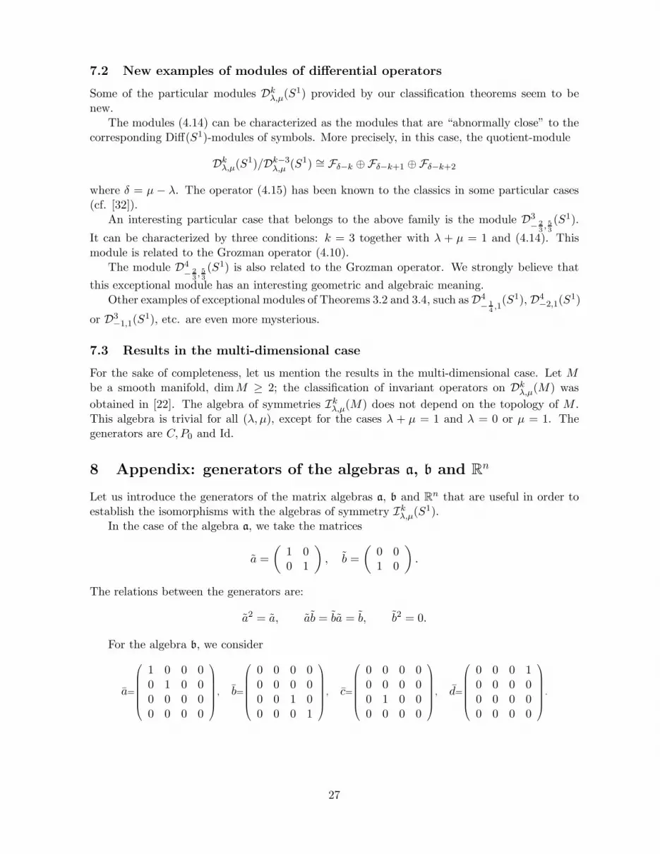
8 Appendix: generators of the algebras a, b and Rn

Let us introduce the generators of the matrix algebras a, b and Rn that are useful in order to

establish the isomorphisms with the algebras of symmetry Ikλ,µ(S1).

In the case of the algebra a, we take the matrices

a =

(

1 00 1

)

, b =

(

0 01 0

)

.

The relations between the generators are:

a2 = a, ab = ba = b, b2 = 0.

For the algebra b, we consider

a=

1 0 0 00 1 0 00 0 0 00 0 0 0

, b=

0 0 0 00 0 0 00 0 1 00 0 0 1

, c=

0 0 0 00 0 0 00 1 0 00 0 0 0

, d=

0 0 0 10 0 0 00 0 0 00 0 0 0

.

27

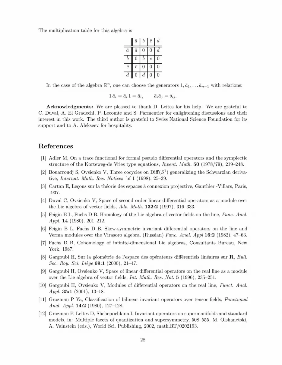
The multiplication table for this algebra is

a b c d

a a 0 0 d

b 0 b c 0

c c 0 0 0

d 0 d 0 0

In the case of the algebra Rn, one can choose the generators 1, a1, . . . an−1 with relations:

1 ai = ai 1 = ai, aiaj = δij .

Acknowledgments: We are pleased to thank D. Leites for his help. We are grateful toC. Duval, A. El Gradechi, P. Lecomte and S. Parmentier for enlightening discussions and theirinterest in this work. The third author is grateful to Swiss National Science Foundation for itssupport and to A. Alekseev for hospitality.

References

[1] Adler M, On a trace functional for formal pseudo differential operators and the symplecticstructure of the Korteweg-de Vries type equations, Invent. Math. 50 (1978/79), 219–248.

[2] Bouarroudj S, Ovsienko V, Three cocycles on Diff(S1) generalizing the Schwarzian deriva-tive, Internat. Math. Res. Notices bf 1 (1998), 25–39.

[3] Cartan E, Lecons sur la theorie des espaces a connexion projective, Gauthier -Villars, Paris,1937.

[4] Duval C, Ovsienko V, Space of second order linear differential operators as a module overthe Lie algebra of vector fields, Adv. Math. 132:2 (1997), 316–333.

[5] Feigin B L, Fuchs D B, Homology of the Lie algebra of vector fields on the line, Func. Anal.Appl. 14 (1980), 201–212.

[6] Feigin B L, Fuchs D B, Skew-symmetric invariant differential operators on the line andVerma modules over the Virasoro algebra. (Russian) Func. Anal. Appl 16:2 (1982), 47–63.

[7] Fuchs D B, Cohomology of infinite-dimensional Lie algebras, Consultants Bureau, NewYork, 1987.

[8] Gargoubi H, Sur la geometrie de l’espace des operateurs differentiels lineaires sur R, Bull.Soc. Roy. Sci. Liege 69:1 (2000), 21–47.

[9] Gargoubi H, Ovsienko V, Space of linear differential operators on the real line as a moduleover the Lie algebra of vector fields, Int. Math. Res. Not. 5 (1996), 235–251.

[10] Gargoubi H, Ovsienko V, Modules of differential operators on the real line, Funct. Anal.Appl. 35:1 (2001), 13–18.

[11] Grozman P Ya, Classification of bilinear invariant operators over tensor fields, FunctionalAnal. Appl. 14:2 (1980), 127–128.

[12] Grozman P, Leites D, Shchepochkina I, Invariant operators on supermanifolds and standardmodels, in: Multiple facets of quantization and supersymmetry, 508–555, M. Olshanetski,A. Vainstein (eds.), World Sci. Publishing, 2002, math.RT/0202193.

28

[13] Kirillov A A, Infinite dimensional Lie groups : their orbits, invariants and representations.The geometry of moments, Lect. Notes in Math., 970 Springer-Verlag (1982), 101–123.

[14] Kirillov A A, Invariant operators over geometric quantities (Russian), in: Current Problemsin Mathematics, 16, 3–29, Akad. Nauk SSSR, VINITI, Moscow, 1980; [English translation:J. Sov. Math 18:1 (1982), 1–21].

[15] Kirillov A A, The orbits of the group of diffeomorphisms of the circle, and local Lie super-algebras, Func. Anal. Appl. 15:2 (1981), 75–76.

[16] Kolar I, Michor P, Slovak J, Natural operations in differential geometry. Springer-Verlag,Berlin, 1993.

[17] Lebedev A, Leites D, Shereshevskii I, Lie superalgebra structures in cohomology spaces ofLie algebras with coefficients in the adjoint representation, math.KT/0404139.

[18] Lecomte P B A, Mathonet P, Tousset E, Comparison of some modules of the Lie algebraof vector fields, Indag. Mathem., N.S. 7:4 (1996), 461–471.

[19] Lecomte P B A, Ovsienko V, Projectively invariant symbol calculus, Lett. Math. Phys. 49:3

(1999), 173–196.

[20] Lecomte P B A, Ovsienko V, Cohomology of the vector fields Lie algebra and modules ofdifferential operators on a smooth manifold, Compos. Math. 124:1 (2000), 95–110.

[21] Martin C, Piard A, Classification of the indecomposable bounded admissible modules overthe Virasoro Lie algebra with weightspaces of dimension not exceeding two, Comm. Math.Phys. 150:3 (1992), 465–493.

[22] Mathonet P, Intertwining operators between some spaces of differential operators on amanifold, Comm. Algebra 27:2 (1999), 755–776.

[23] Mathonet P, Geometric quantities associated to differential operators, Comm. Algebra 28:2

(2000), 699–718.

[24] Ovsienko O, Ovsienko V, Lie derivatives of order n on the line. Tensor meaning of theGelfand-Dikii bracket, Adv. Soviet Math. 2 (1991), 221–231.

[25] Ovsienko V, Tabachnikov S, Projective differential geometry old and new: from theSchwarzian derivative to cohomology of diffeomorphism groups, Cambridge UniversityPress, 2004.

[26] Peetre J, Une caracterisation abstraite des operateurs differentiels, Math. Scand. 7 (1959),211–218 and 8 (1960), 116–120.

[27] Rudakov A N, Irreducible representations of infinite-dimensional Lie algebras of Cartantype, Izv. Akad. Nauk SSSR Ser. Mat. 38 (1974), 835–866.

[28] Segal G B, Unitary representations of some infinite dimensional groups, Comm. Math. Phys.80:3 (1981), 301–342.

[29] Terng C L, Natural vector bundles and natural differential operators, Amer. J. Math. 100:4

(1978), 775–828.

[30] Veblen O, Differential invariants and geometry, Atti del Congresso Internazionale deiMatematici, Bologna, 1928.

[31] Weyl H, The Classical Groups, Princeton University Press, 1946.

[32] Wilczynski, E J Projective differential geometry of curves and ruled surfaces, Leipzig -Teubner, 1906.

29