Quasicritical brain dynamics on a nonequilibrium Widom line

Quasi-Critical Brain Dynamics on a Non-Equilibrium Widom Line

Rashid V. Williams-Garcıa,∗ Mark Moore, John M. Beggs, and Gerardo OrtizDepartment of Physics, Indiana University, Bloomington, Indiana 47405, USA

(Dated: March 29, 2014)

Is the brain really operating at a critical point? We study the non-equilibrium properties of aneural network which models the dynamics of the neocortex and argue for optimal quasi-criticaldynamics on the Widom line where the correlation length is maximal. We simulate the network andintroduce an analytical mean-field approximation, characterize the non-equilibrium phase transition,and present a non-equilibrium phase diagram, which shows that in addition to an ordered anddisordered phase, the system exhibits a quasiperiodic phase corresponding to synchronous activityin simulations which may be related to the pathological synchronization associated with epilepsy.

PACS numbers: 87.19.lj, 64.60.aq, 64.60.av, 87.19.ll

Recent experimental evidence from a variety of liv-ing neural networks suggests that the brain may beoperating at or near a critical point, poised betweendisordered (“subcritical”) and ordered (“supercritical”)phases where cascades of activity are damped or ampli-fied, respectively [1–9]. At this interface, neural networksare expected to produce avalanches of activity whose sizeand duration probability distributions follow power laws,as a distinctive feature of critical phenomena is scale-invariance [10–13]. Theory and simulations conjecturedthat neural networks poised at a critical point wouldhave optimal information transmission [1], informationstorage [11, 14], computational power [15, 16], dynamicrange [16–24], and learning capabilities [25], while pro-viding flexible, yet stable dynamics [11, 26]. Several ex-periments claim results consistent with these predictions[27–29], lending plausibility to the criticality hypothesisof brain function [30].

Here we introduce and analyze the so-called corti-cal branching model (CBM), a non-equilibrium stochas-tic cellular automaton capturing many features of neu-ral network data [11, 14, 31], and develop an analyticalmean-field approximation in the form of an autonomousnonlinear discrete dynamical map of first order and di-mension given by the integer-valued refractory period.Using this approximation, we show that a continuousphase transition occurs (in the thermodynamic limit)only when external driving, which we model as the spon-taneous activation of network elements, is absent.

When external driving is present (and the refrac-tory period small), the system does not display non-analyticities. We hence posit that true criticality isnot attainable by living neural networks (which exhibitspontaneous activity) and argue for an extension (anda more proper quantitative formulation) of the critical-ity hypothesis: a quasi-criticality hypothesis. Quasi-critical behavior can be attained along a line of max-imum (though finite) dynamical susceptibility (a non-

∗ Electronic address: [email protected]

equilibrium Widom line) and, equivalently, maximumcorrelation length. Increasing the refractory periodat large values of the branching parameter, induces aquasiperiodic phase in the mean-field which correspondsto synchronous activation in simulations [33]. Resultsof our numerical simulations are qualitatively consistentwith the mean-field calculations. Because spontaneousactivation rates in neural networks are readily manipu-lated experimentally [34, 35], our predictions could soonbe tested; it is worth noting that our approach can be ex-tended to other systems, such as the SIRS compartmentaldisease epidemic model, which shares many similaritieswith the CBM [36].

We next introduce details of the CBM. Consider arandom directed network, or graph, of N nodes, whereeach node has its own local neighborhood of interac-tions; connections are established and kept fixed through-out the dynamics, as in quenched disorder. Randomnetworks can either be strongly-connected–in which casethere exists a path (never running anti-parallel throughdirected connections) from any node in the network toany other node on the network (through possibly manyintermediaries)–or weakly-connected–in which case thenetwork contains subgraphs and is said to not be fully-connected. Networks are generated randomly and testedfor connectedness by examining the corresponding adja-cency matrix associated with its graph. In this study,we only consider strongly-connected networks, implyingthat their adjacency matrices are irreducible [37].

Internodal connections are weighted, with elements ofthe weighted adjacency matrix P = {Pij ≤ 1} represent-ing the probability Pij = κpnij that a connection fromnode i to node j will transmit activity, with

pnij =e−Bnij

∑kinn=1 e

−Bn, (1)

where κ is the branching parameter (which is equivalentto the Perron-Frobenius eigenvalue of P ), kin is the in-degree of each node, B is the connection strength bias,and nij ∈ {1, · · · , kin} ranks each connection inboundat node j by strength, e.g. nij = 1 corresponds to the

arX

iv:1

405.

6232

v1 [

q-bi

o.N

C]

23

May

201

4

2

strongest connection inbound at node j. We constrainκ to the range (0, κmax], where the upper bound is given

by κmax = eB∑kinn=1 e

−Bn and the lower bound corre-sponds to a fully-disconnected network. Close to andabove κ = κmax, the CBM produces constant activity,not avalanches. It had previously been determined thatfor a network of N = 60 nodes, each with a fixed kin = 10,that the values B = 1.2 and B = 1.6 allowed for a rea-sonable fit to the local field potential (LFP) dynamicsrecorded from living neural networks [14]; we present ourprimary simulation results with B = 1.4 and kin = 3.

The state of each node i is determined by a dynamicalstate variable zi ∈ S, S = {0, 1, 2, . . . , τr}, i = 1, · · · , N ,where τr ≥ 1 is the integer-valued refractory period,i.e. the number of timesteps following activation dur-ing which a node cannot be made to activate. A node iis said to be active when zi = 1, inactive (i.e. quiescent)when zi = 0, and refractory at any other value. Nodescan only be active for a single timestep at a time.

The system is driven by the spontaneous activation ofa node, which occurs with probability ps. The number oftimesteps between spontaneous activations follows a dis-crete probability distribution of our choice [33]: a Pois-son distribution with rate 1/(psN) allows for a greaterseparation of driving and relaxation timescales, such asthat seen in instances of self-organized criticality (SOC)[38, 39], thus minimizing the occurrence of overlappingavalanches; whereas by using a geometric distributionwith success probability psN , avalanches are more likelyto overlap and contain spontaneous events. Simulationresults presented herein utilize Poisson-distributed spon-taneous events to generate avalanches.

A node can also be driven to activate by another nodeconnected to it with probabilities given by Eq. (1), butonly if the driving node was active and the driven nodequiescent in the preceding timestep. Regardless of themethod of stochastic activation, a node’s dynamical vari-able zi changes deterministically following activation, in-creasing by 1 every timestep until zi = τr is reached,after which the node becomes quiescent (zi = 0) until itis stochastically activated once again. Thus, each statevariable zi represents a clock degree of freedom. Forexample, consider a node i with τr = 3: following thetimestep during which it was active, this node will be-come refractory, its state deterministically changing fromzi = 2 to zi = 3, and finally to zi = 0. Refer to [33] for adetailed algorithm of the CBM.

Clusters of activation exhibited by the CBM mimicspatio-temporal patterns (neuronal avalanches) observedin living neural networks [11, 14]. We explore their prop-erties by first defining the density of active nodes at timet, ρ1(t), as

ρ1(t) =1

N

N∑

i=1

δzi(t),1. (2)

We often consider its time average, ρ1 = 〈ρ1(t)〉t. Thedynamical susceptibility χ, associated with the density ofactive nodes, corresponds to the fluctuation of ρ1(t), χ =N [〈ρ2

1(t)〉t−(ρ1)2], and quantifies the dynamical responseof the system. The correlation length associated withχ will play an important role in establishing the quasi-criticality hypothesis. In the mean-field approximationdefined below, χ will be determined from the expressionlimps→0 ∂ρ1/∂ps.

Periods of inactivity (ρ1 = 0) are punctuated by pe-riods of activity (ρ1 6= 0) which constitute avalanches.The properties of these avalanches are encoded in theavalanche shape, which we define as the density of ac-tive nodes over the duration of an avalanche, resemblingdefinitions given in previous studies [40]. The avalancheshape vector Xq gives the shape of the qth avalanche:

Xq(φ) =

N∑

i=1

δzi(t0q+φ−1),1, (3)

where t0q is its starting time, dq is its duration, andφ = [1, dq] ∈ Z+ indexes the number of timesteps withinthe avalanche. From this, we write the size of the qth

avalanche as sq =∑dqφ=1Xq(φ).

Avalanche size and duration probability distributionsare conjectured [1] to follow power laws, P (s) ∝ s−τ andP (d) ∝ d−α. In simulated and living neural networks,values of these exponents have been found to be τ ≈1.5 and α ≈ 2 for LFP data and τ ≈ 1.6 and α ≈ 1.7for neuronal spike data; results which have been used tosupport the criticality hypothesis [10–12].

In order to gain a deeper understanding of our CBMand its non-equilibrium phase diagram, we next developan analytical mean-field approximation starting from theChapman-Kolmogorov equation [32, 33]. The mean-fieldis local in nature and so involves a single, representativenode with kin incoming connections, each with connectionstrength given by κpm, where m = {1, . . . , kin}.

We consider the probabilities xz that this node is in anystate z ∈ S, thus yielding a system of τr + 1 equations.The restriction that, at any iteration t, these probabilitiesmust add to one (

∑τrz=0 xz(t) = 1) reduces the system to

τr equations. An equivalent mean-field approximationcan be formulated as a non-Markovian τrth-order map inone dimension. For kin = 1, the mean-field equations are

x1(t+ 1) =

(1−

τr∑

z=1

xz(t)

)[g x1(t) + ps]

xz(t+ 1) = xz−1(t), for z = {2, · · · , τr}, (4)

where g = κp1(1 − ps) and since kin = 1, then κmax = 1and p1 = 1.

Fixed points x∗1 of this map give approximations of thenumbers of nodes in each of the various states. Stabil-ity of each x∗1 is established as usual by calculating the

3

eigenvalues of the Jacobian matrix associated with themap. The stable eigenspace is spanned by the eigen-vectors whose eigenvalues have modulus smaller than 1;eigenvectors with eigenvalues of modulus larger than 1span the unstable eigenspace.

When ps = 0, Eq. (4) gives two fixed points, x∗1 = 0and x∗1 = (1 − 1/κp1)/τr. The vanishing fixed point be-comes unstable when κ > 1 and so we find that thestable fixed point, which provides the mean-field ap-proximation to the time-averaged density of active nodes(ρ1 ≈ x∗1), acts as a Landau order parameter, i.e. ρ1 = 0for κ ≤ 1 and ρ1 > 0 for κ > 1, with the criticalpoint at κc = 1. We find the critical exponent β = 1:x∗1 ∝ (κ − κc)β for κ > 1. Calculating the susceptibil-ity, χ = limps→0 ∂ρ1/∂ps, we find that it diverges at κcwith exponent γ′ = 1 for κ < 1: χ ∝ (κc − κ)−γ

′. For

κ > 1, it diverges with exponent γ = 1: χ ∝ (κ− κc)−γ .It is remarkable to note that this mean-field approxima-tion to the CBM in the case kin = 1 and τr = 1 is thediscrete-time equivalent of the directed percolation mean-field equation,

∂tρ1(t) = −gρ1(t)2 + (g − 1− ps)ρ1(t) + ps, (5)

as given in [41], where ps plays the role of an externalfield. These two seemingly different processes thereforebelong to the same mean-field universality class.

In the case kin = 2, the mean-field approximation leadsto the non-linear discrete-time t map:

x1(t+ 1) =

(1−

τr∑

z=1

xz(t)

)[−ax2

1(t) + bx1(t) + ps]

xz(t+ 1) = xz−1(t), for z = {2, · · · , τr}, (6)

where a = κ2p1p2(1−ps) and b = κ(1−ps). In the absenceof spontaneous activity (ps = 0), we have a vanishingfixed point (x∗1 = 0) and a pair of real, non-zero fixedpoints given by

x∗1± =κp1p2 + τr ±

√(κp1p2 + τr)2 − 4p1p2τr(κ− 1)

2κp1p2τr.

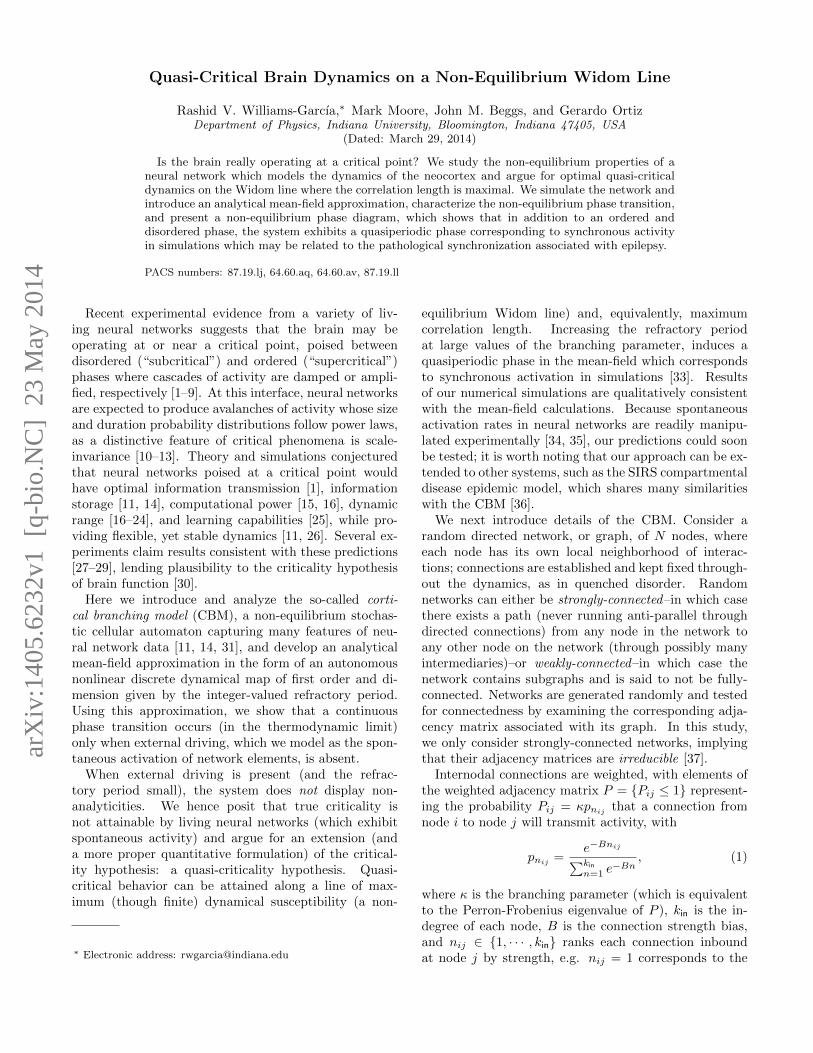
(7)Stability of fixed points again changes at κc = 1; thefixed point x∗1 = 0 is stable when κ < κc and x∗1− isstable when κ > κc. The susceptibility χ = ∂x∗1/∂psdiverges at κc when ps → 0. Interestingly, the criticalexponents remain the same, β = 1, γ′ = 1, and γ = 1,characterizing this second-order transition. When ps 6= 0(and for small values of τr), a single fixed point is stableacross κ = 1 and so χ no longer diverges, i.e. the phasetransition disappears, giving way to a crossover region.The non-equilibrium phase diagram can be seen in Fig.1. To give an idea of the shape of the dynamical suscepti-bility, we have included light-blue bubbles with diameterlogarithmically-scaled to its magnitude, and blue hori-zontal lines indicating its width at half-maximum which

encompasses the quasi-critical region. We have used thevalue B = 0.5 for presentation purposes, as it allows thereader to better view the full extent of the quasiperiodicphase boundary when κ is large; note that with kin = 2,κmax(B = 1.4) ≈ 1.247 while κmax(B = 0.5) ≈ 1.607.Changes in B had no discernible impact on the phase di-agram. For a fixed value of τr, we can identify the peakin the susceptibility (and correlation length), defining anon-equilibrium Widom line in the τr–κ plane; for theequivalent equilibrium Widom line see [42].

For large τr, the fixed point x∗1− loses stability and x1(t)subsequently exhibits “oscillatory” behavior lacking pe-riodic points [33]; similar quasiperiodic phenomena hadpreviously been observed in SIRS-like models [44]. Thisquasiperiodic phase was found to diminish with increas-ing ps, eventually disappearing at ps ≈ 7 × 10−3. Os-cillatory behavior emerging at large refractory periodshad previously been observed in neural network mod-els [17, 43, 45], but the quasiperiodic behavior observedhere and in [44] was not found. It should be noted thatCurtu and Ermentrout’s model involved both excitatoryand inhibitory elements whereas the CBM only involvesexcitatory elements [45]. 3

the eigenvalues of the Jacobian matrix associated withthe discrete map. The stable eigenspace is spanned bythe eigenvectors whose eigenvalues have modulus smallerthan 1, while eigenvectors with eigenvalues larger than 1define the unstable eigenspace.

In the absence of spontaneous activation, i.e. ps = 0,Eq. (4) gives two fixed points, x∗1 = 0 and x∗1 = (1 −1/κp1)/τr. The vanishing fixed point becomes unstablewhen κ > 1 and so we find that the stable fixed point,which provides the mean-field approximation to the time-averaged density of active nodes (ρ1 ≈ x∗1), acts as aLandau order parameter, i.e., ρ1 = 0 for κ ≤ 1 and ρ1 > 0for κ > 1, with the critical point at κc = 1. We find thecritical exponent β = 1: x∗1 ∝ (κ − κc)

β for κ > 1.Calculating the susceptibility χ = limps→0 ∂ρ1/∂ps, wefind that it diverges at κc with exponent γ′ = 1 for κ < 1:χ ∝ (κc − κ)−γ

′. For κ > 1, it diverges with exponent

γ = 1: χ ∝ (κ−κc)−γ . It is remarkable to note that thismean-field approximation to the CBM in the case kin = 1and τr = 1 is the discrete-time equivalent of the directedpercolation mean-field equation,

∂tρ1(t) = −gρ1(t)2 + (g − 1− ps)ρ1(t) + ps, (5)

as given in [30], where ps plays the role of an externalfield. These two seemingly different processes thereforebelong to the same mean-field universality class.

In the case kin = 2, the mean-field approximation leadsto the non-linear discrete-time t map:

x1(t+ 1) =

(1−

τr∑

z=1

xz(t)

)[−ax21(t) + bx1(t) + ps]

xz(t+ 1) = xz−1(t), for z = {2, · · · , τr}, (6)

where a = κ2p1p2(1−ps) and b = κ(1−ps). In the absenceof spontaneous activity (ps = 0), we have a vanishingfixed point (x∗1 = 0) and a pair of real, non-zero fixedpoints given by

x∗1± =κp1p2 + τr ±

√(κp1p2 + τr)2 − 4p1p2τr(κ− 1)

2κp1p2τr.

(7)Once again, stability of fixed points changes at κc = 1;the fixed point x∗1 = 0 is stable when κ < κc and x∗1− isstable when κ > κc. The susceptibility χ = ∂x∗1/∂psdiverges at κc when ps → 0. Interestingly, the crit-ical exponents remain the same, β = 1, γ′ = 1, andγ = 1, characterizing this second-order mean-field tran-sition. When ps 6= 0 (and for small enough values of τr),a single fixed point is stable across κ = 1 and so the sus-ceptibility no longer diverges, i.e., the phase transitiondisappears, giving way to a crossover region. Fig. 1 dis-plays the resulting non-equilibrium phase diagram. For afixed value of τr, we can identify the peak in the suscep-tibility (and therefore the correlation length), defining anon-equilibrium Widom line in the τr–κ plane; for theequivalent equilibrium Widom line see [31]. To give anidea about the width of the susceptibility peak we plot

20

40

60

80

100

τ r

ps = 0 ps = 10−5

0.6 0.8 1.0 1.2 1.4 1.6

20

40

60

80

100

κ

τ r

ps = 10−4

0.6 0.8 1.0 1.2 1.4 1.6κ

ps = 10−3

FIG. 1. Non-equilibrium mean-field phase diagram for kin = 2and B = 0.5, at selected values of the spontaneous activa-tion probability ps. The white region corresponds to the sub-critical disordered phase with a vanishing stable fixed point;the light-gray region corresponds to the supercritical orderedphase with a nonzero stable fixed point; the dark-gray regioncorresponds to an “oscillatory” quasi-periodic phase, whereall fixed points are unstable. Solid black lines are lines ofnon-analyticity, and thus represent phase boundaries.

horizontal blue lines (color available online) whose lengthindicate the width at half-maximum; this represents thequasi-critical region.

With larger values of the refractory period τr, we finda region in which there are no stable fixed points, insteadfinding x1(t) to exhibit “oscillatory” behavior; periodicpoints are also not found and instead x1(t) appears tovary chaotically within a sinusoidal envelope [26]. Thisquasi-periodic phase was found to diminish with increas-ing ps, eventually disappearing at ps ≈ 7 × 10−3. Os-cillatory behavior emerging at large refractory periodshas previously been observed in neural network models[16, 32], but the quasi-periodic behavior observed herewas not realized before. It should be noted that Curtuand Ermentrout’s model involved both excitatory andinhibitory connections whereas the CBM only involvesexcitatory connections [32].

We note that since the mean-field approximation elim-inates fluctuations, it is not useful in rigorously analyzingthe physics of the avalanches associated with our model.Therefore, we next describe the results of our CBM simu-lations. With τr = 1, simulations were performed for sys-tem sizes N = {32, 64, 96, 128} and spontaneous activa-tion probabilities ps = {10−5, 10−4, 10−3} at each value ofκ = [0.8, 1.3] with a step size δκ = 0.01. Ten simulationswere performed on different random networks until 106

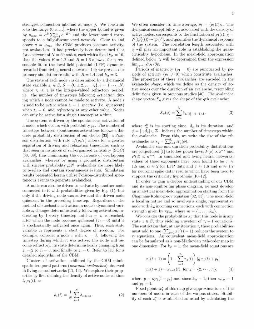
avalanches were generated at each value of κ; avalanchedurations were limited to 105 timesteps. Note that withB = 1.4 and kin = 3, κmax ≈ 1.307. We determined thetime-averaged density of active nodes ρ1 as well as thesusceptibility χ, each as functions of κ for the various val-ues of ps (see Fig. 2). The susceptibility peaks at quasi-

FIG. 1. (Color online) Non-equilibrium mean-field phase di-agram for kin = 2, at selected values of ps. The white regionrepresents the disordered phase; the light-gray region repre-sents the ordered phase, and the dark-gray region representsthe quasiperiodic phase. Solid black lines are lines of non-analyticity, and thus represent phase boundaries.

We note that since the mean-field approximation elim-inates fluctuations, it is not useful in rigorously an-alyzing the physics of the avalanches associated withour model. Therefore, we next describe the results ofour CBM simulations. With τr = 1, simulations wereperformed for system sizes N = {32, 64, 96, 128} andps = {10−5, 10−4, 10−3} at each value of κ = [0.8, 1.3]with a step size δκ = 0.01. Simulations were performedon ten different random networks until 106 avalancheswere generated at each value of κ; avalanche durations

4

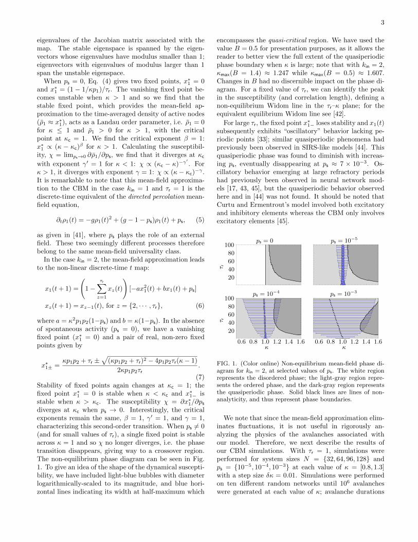
were limited to 105 timesteps. Note that with B = 1.4and kin = 3, κmax ≈ 1.307. We determined the time-averaged density of active nodes ρ1 as well as the dy-namical susceptibility χ, each as functions of κ for thevarious values of ps (see Fig. 2). The susceptibility peaksat quasi-critical points κw defining a non-equilibriumWidom line in the ps–κ plane. Much of the disagreementbetween the mean-field and simulation results is due tofinite-size effects. If we were interested in the thermody-namic limit, we would need much larger system sizes; thisis, however, numerically-intensive and computationally-complex. Avalanche size distributions at these κw ex-hibit quasi-power-law behavior over a maximum numberof decades (see Fig. 3). 1

κ/κw

χ/χ(m

ax)

N = 128

0.8 0.9 1.0 1.10

0.2

0.4

0.6

0.8

1

κ/κw

ρ1/ρ(m

ax)

1

0.8 1.00

0.5

1

ps = 10−5

ps = 10−4

ps = 10−3

///

FIG. 2. Dynamical susceptibility χ and ρ1 (inset) resultsfrom simulation (data markers) and mean-field approximation(lines). Results are normalized to their maximal values andplotted against κ normalized to the quasi-critical point κw atps = 10−5. For simulations, we find κw to be 1.10, 1.12, and1.17 at ps = 10−3, 10−4, and 10−5, respectively

At values of τr and κ comparable to those at which themean-field exhibits quasiperiodicity, an oscillatory syn-chronization phenomenon is observed in simulations [33].The significance of this quasiperiodic phase in terms ofthe behavior of living neural networks is not yet under-stood. Previous studies have found neuronal refractoryperiods to increase as a result of the axonal demyelinationassociated with multiple sclerosis [46–48]–a disease whichis correlated with an unexplained increased incidence ofepileptic seizures [49]. Perfusion of glutamate receptoragonists (such as kainic acid, KA) has been found to de-crease neuronal refractory periods, while glutamate re-ceptor antagonists (such as 6-cyano-7-nitroquinoxaline-2,3-dione, CNQX) were found to increase them [50].Paradoxically, both KA and CNQX have been used toinduce in vitro seizure-like activity [51, 52]. So while the

1

Avalanche Size, s

P(s)

N = 128, ps = 10−4

100 102 104 106

10−6

10−4

10−2

100

κ = 1.08κ = κw = 1.12

κ = 1.16

FIG. 3. Logarithmically-binned avalanche size probabilitydistributions P (s) at various values of κ. The dashed linerepresents a power law with exponent τ = 1.6.

oscillations observed in simulations are possibly relatedto the pathological synchronization typically associatedwith epilepsy, we note that synchronization in epilepsy iscomplex and not fully understood [53].

We remark that in changing τr, we are manipulatingan intrinsic timescale of the system. There are a num-ber of ways living neural networks could adjust such atimescale: as a result of widespread neuronal activationor synchronization, or perhaps by changing the balanceof excitation and inhibition. Indeed, the existence ofmultiple timescales is important in SOC and we identifyfour timescales in our model, two of which we manipulatehere: (1) the driving timescale associated with ps, (2) therelaxation timescale associated with the avalanche dura-tion d, (3) the refractory timescale associated with τr,and (4) the transmission timescale, i.e. the time duringwhich a signal is in transit from its origin to its destina-tion node.

An earlier experimental paper assumed that neuralnetworks displayed a form of SOC [1]. A key require-ment of SOC is a separation of timescales [38]. Indeedisolated networks used for in vitro preparations typicallyshow intervals of many seconds between network burststhat initiate avalanches, while avalanches themselves lasttens to hundreds of milliseconds [54]. This separation isnot clearly seen with in vivo preparations, where eachneural network receives many synaptic inputs from otherintact brain regions. In the context of the model pre-sented here, in vitro preparations would have ps ≈ 0;in vivo preparations would however have ps > 0. Theimportant consequence of this is that in vivo networkswould not operate at criticality (which can only occurwhen ps = 0), but would instead perhaps operate atquasi-criticality, along the non-equilibrium Widom line.

5

We suggest that this framework could explain why powerlaws from spiking activity have rarely been found in vivo[55], although there have been numerous reports of themin vitro [2, 4, 34].

The authors would like to thank J. Kertesz, K.M. Pil-grim, and A. Vespignani for helpful discussions.

[1] J.M. Beggs and D. Plenz, J. Neurosci. 23, 11167 (2003).[2] N. Friedman et al., Phys. Rev. Lett. 108, 208102 (2012).[3] M.G. Kitzbichler et al., PLoS Comput. Biol. 5, e1000314

(2009).[4] V. Pasquale et al., Neuroscience 153, 1354 (2008).[5] T. Petermann et al., Proc. Nat. Acad. Sci. 106, 15921

(2009).[6] S.S. Poil, A. van Ooyen, and K. Linkenkaer-Hansen,

Hum. Brain Mapp. 29, 770 (2008).[7] V. Priesemann et al., PLoS Comput. Biol. 9, e1002985

(2013).[8] T.L. Ribeiro et al., PLoS ONE 5, e0014129 (2010).[9] O. Shriki et al., J. Neurosci. 33, 7079 (2013).

[10] A. Levina, J.M. Herrmann, and T. Geisel, Nat. Phys. 3,857 (2007).

[11] C. Haldeman and J.M. Beggs, Phys. Rev. Lett. 94,058101 (2005).

[12] T.E. Harris, The Theory of Branching Processes (DoverPublications, New York, 1989).

[13] H. Nishimori and G. Ortiz, Elements of Phase Transi-tions and Critical Phenomena (Oxford University Press,New York, 2011).

[14] W. Chen et al., BMC Neurosci. 11, 3 (2010).[15] N. Bertschinger and T. Natschlager, Neural Comput. 16,

1413 (2004).[16] L.L. Gollo et al., Sci. Rep. 3, 3222 (2013).[17] O. Kinouchi and M. Copelli, Nat. Phys. 2, 348 (2006).[18] D.B. Larremore et al., Phys. Rev. Lett 106, 058101

(2011).[19] R. Publio et al., PLoS ONE 7, e48517 (2012).[20] For a two-state cellular automata on a regular (non-

random) network, see: K. Manchanda et al., Phys. Rev.E 87, 012704 (2013).

[21] T.S. Mosqueiro and L.P. Maia, Phys. Rev. E 88, 012712(2013).

[22] L. Wang et al., Chin. Phys. Lett. 30, 070506 (2013).[23] S. Pei et al., Phys. Rev. E 86, 021909 (2012).[24] L.L. Gollo et al., Phys. Rev. E 85, 011911 (2012).[25] L. de Arcangelis and H.J. Herrmann, Proc. Nat. Acad.

Sci. 107, 3977 (2010).[26] M.O. Magnasco, O. Piro, and G.A. Cecchi, Phys. Rev.

Lett. 102, 258102 (2009).[27] W.L. Shew et al., J. Neurosci. 29, 15595 (2009).[28] W.L. Shew et al., J. Neurosci. 31, 55 (2011).[29] G. Solovey et al., Front. Integr. Neurosci. 6, 44 (2012).[30] J.M. Beggs, Philos. Transact. A Math. Phys. Eng. Sci.

366, 329 (2008).[31] S. Pajevic and D. Plenz, PLoS Comput. Biol. 5, e1000271

(2009).[32] A. Deutsch and S. Dormann, Cellular Automaton Mod-

eling of Biological Pattern Formation: Characterization,Applications, and Analysis (Birkhauser, Boston, 2005).

[33] See Supplemental Material below for a detailed descrip-

tion of the CBM, the mean-field approximation, and ad-ditional figures.

[34] A. Mazzoni et al., PLoS ONE 2, e439 (2007).[35] D.E. Gunning et al., J. Neural Eng. 10, 016007 (2013).[36] R.M. Anderson and R.M. May, Nature (London) 280,

361 (1979).[37] D.B. Larremore et al., Phys. Rev. E 85, 066131 (2012).[38] H. J. Jensen, Self-Organized Criticality: Emergent Com-

plex Behavior in Physical and Biological Systems (Cam-bridge University Press, New York, 1998).

[39] A. Vespignani and S. Zapperi, Phys. Rev. E 57, 6345(1998).

[40] J.P. Sethna et al., Nature (London) 410, 242 (2001).[41] M. Henkel, H. Hinrichsen, and S. Lubeck, Non-

Equilibrium Phase Transitions, Vol. 1 (Springer, Dor-drecht, 2008).

[42] L. Xu et al., Proc. Nat. Acad. Sci. 102, 16558 (2005).[43] F. Rozenblit and M. Copelli, J. Stat. Mech. 2011, P01012

(2011).[44] M. Girvan et al., Phys. Rev. E 65, 031915 (2002).[45] R. Curtu and B. Ermentrout, J. Math. Biol. 43, 81

(2001).[46] F.N. Quandt and F.A. Davis, Biol. Cybern. 67, 545

(1992).[47] P.A. Felts, T.A. Baker, and K.J. Smith, J. Neurosci. 17,

7267 (1997).[48] Z.H. Luo et al., J. Innov. Opt. Health Sci. 7, 1330003

(2014).[49] B.J. Kelley and M. Rodriguez, CNS Drugs 23, 805

(2009).[50] R. Dawkins and W.F. Sewell, J. Neurophysiol. 92, 1105

(2004).[51] A. Bragin et al., Epilepsia 40, 127 (1999).[52] W. van Drongelen et al., IEEE T. Neur. Sys. Reh. 13,

236 (2005).[53] P. Jiruska et al, J. Physiol. 591, 787 (2013).[54] F. Lombardi et al., Phys. Rev. Lett. 108, 228703 (2012).[55] G. Hahn et al., J. Neurophysiol. 104, 331 (2010).

6

SUPPLEMENTAL MATERIALS

Algorithm of the Random Neighbor DiscreteCortical Branching Model (CBM)

We summarize the dynamics of the random neighbordiscrete CBM with the following algorithm:

1. Initialization. Prepare nearest neighbor connec-tions by randomly assigning connections betweennodes while keeping the in-degree kin fixed (par-allel connections are allowed; loops are not) andprepare connection strengths Pij [see main arti-cle]. Initialize the system in the only stable con-figuration, i.e. zi = 0 for every node i. Pre-pare the first spontaneous activation(s) at t =1 and subsequent spontaneous activation timesby drawing inter-activation intervals ∆ts from achosen discrete distribution, either Poisson, i.e.P (∆ts) = (psN)−∆tse−1/psN/∆ts!, or geometric,i.e. P (∆ts) = (1− psN)∆ts−1psN .

2. Drive. For each spontaneous activation time equalto the current timestep t, randomly select a nodej to activate, zj(t) → 1; if however node j wasnot initially quiescent (i.e. zj(t) = 0), then sponta-neous activation does not occur at node j.

3. Relaxation. Any nodes i for which zi(t − 1) 6= 0:zi(t) = zi(t − 1) + 1. If zi(t) > τr, then zi(t) → 0.Node j, having been active at timestep t, will in-fluence the activity of a neighboring node k attimestep t + 1 with probability Pjk, but only ifzk(t+ 1) = 0: zk(t+ 1)→ zk(t+ 1) + 1.

4. Iteration. Start the next time-step: Return to 2.

Significant Quantities and Relations

For a CBM simulation on a network of N nodes, wedefine the density of active nodes at a time t, ρ1(t), as

ρ1(t) =1

N

N∑

i=1

δzi(t),1 (8)

and identify its time-average ρ1 = 〈ρ1(t)〉t as the orderparameter in the thermodynamic limit and as ps → 0.Periods of inactivity (ρ1 = 0) are punctuated by periodsof activity (ρ1 6= 0), i.e. avalanches. The propertiesof these avalanches are encoded in the avalanche shape,which we define as the density of active nodes over theduration of an avalanche. The avalanche shape vectorXq gives the shape of the qth avalanche:

Xq(φ) =

N∑

i=1

δzi(t0q+φ−1),1 (9)

1

P12P15

P23

P24

P31

P42

P43

P45

P51

P54

z1 =0

12

345

z2 =

012

345

z3 =0

12

345

z4 = 012

345

z5 =

012

345

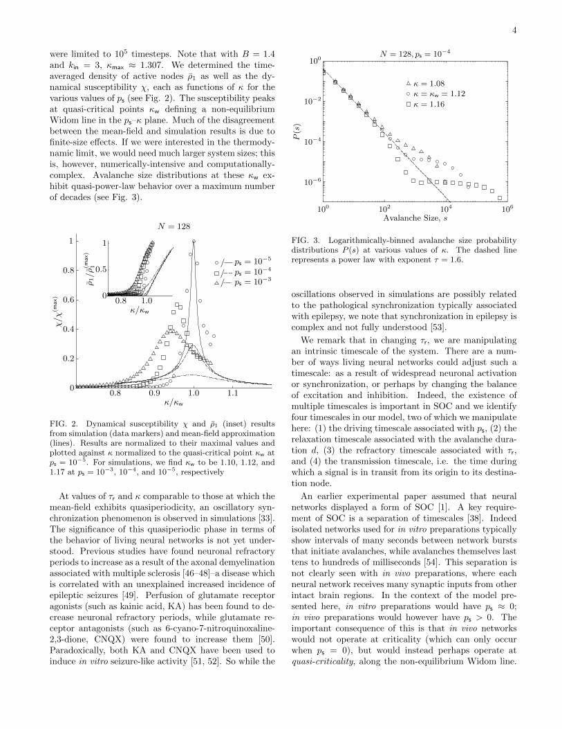
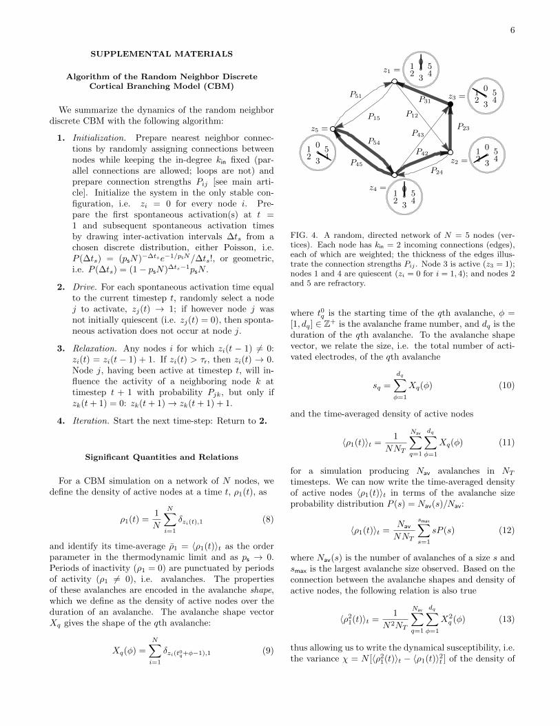
FIG. 4. A random, directed network of N = 5 nodes (ver-tices). Each node has kin = 2 incoming connections (edges),each of which are weighted; the thickness of the edges illus-trate the connection strengths Pij . Node 3 is active (z3 = 1);nodes 1 and 4 are quiescent (zi = 0 for i = 1, 4); and nodes 2and 5 are refractory.

where t0q is the starting time of the qth avalanche, φ =[1, dq] ∈ Z+ is the avalanche frame number, and dq is theduration of the qth avalanche. To the avalanche shapevector, we relate the size, i.e. the total number of acti-vated electrodes, of the qth avalanche

sq =

dq∑

φ=1

Xq(φ) (10)

and the time-averaged density of active nodes

〈ρ1(t)〉t =1

NNT

Nav∑

q=1

dq∑

φ=1

Xq(φ) (11)

for a simulation producing Nav avalanches in NTtimesteps. We can now write the time-averaged densityof active nodes 〈ρ1(t)〉t in terms of the avalanche sizeprobability distribution P (s) = Nav(s)/Nav:

〈ρ1(t)〉t =Nav

NNT

smax∑

s=1

sP (s) (12)

where Nav(s) is the number of avalanches of a size s andsmax is the largest avalanche size observed. Based on theconnection between the avalanche shapes and density ofactive nodes, the following relation is also true

〈ρ21(t)〉t =

1

N2NT

Nav∑

q=1

dq∑

φ=1

X2q (φ) (13)

thus allowing us to write the dynamical susceptibility, i.e.the variance χ = N [〈ρ2

1(t)〉t − 〈ρ1(t)〉2t ] of the density of

7

active nodes, in terms of the avalanche shape vector andsize by making use of Eqs. (10), (11), and (13):

χ =1

NNT

Nav∑

q=1

dq∑

φ=1

X2q (φ)− 1

NT

(Nav∑

q=1

sq

)2 (14)

The Mean-Field Approximation

In the mean-field approximation, CBM dynamics areapproximated by a single node and its local neighborhoodof interaction; only connections from the neighborhoodto this single, representative node are made. The cellu-lar automaton (CA) rules we have described are approxi-mated by a Markovian stochastic process and so the prob-ability that a particular node will be in a specific stateis given by the Chapman-Kolmogorov equation [32]. Wethus have the following

P (zr(t+ 1) = z) =∑

z∈SNW (z→ z)

kin∏

i=0

P (zi(t)) (15)

where z is an element in the state space S = {0, ..., τr}, rspecifies the position of a node (with the representativenode located at r = 0), kin is the in-degree of the repre-sentative node (i.e. the number of neighboring nodes),and z = (z0, ..., zkin) is the configuration of the localneighborhood including the representative node. We con-sider the transition probabilities W (z→ z) to be transla-tionally invariant, as is appropriate within the mean-fieldapproximation.

The probability P (zr(t) = z) can be identified as thefraction of nodes xz(t) in state z, i.e. P (zr(t) = z) =xz(t) =

∑r xz(r, t)/(kin + 1), where xz(r, t) = δzr(t),z.

For example, x1(t) gives the fraction of active nodes at atime t. Eq. (15) hence becomes

xz(t+ 1) =∑

z∈SNW (z→ z)

kin∏

i=0

xzi(t) (16)

We can thus find a set of iterative maps which allow us tocalculate the mean-field densities of quiescent, active, andrefractory nodes, however, we are primarily interested inthe density of active nodes. Because a node must bequiescent at t to become active at t + 1, we write theabove as

x1(t+ 1) =

(1−

τr∑

z=1

xz(t)

) ∑

z′∈SkinW (z′ → 1)

kin∏

i=1

xzi(t)

(17)where z′ is the configuration of the local neighborhood,excluding the representative node, i.e. z′ = (z1, ..., zkin).Using the CA rules for our CBM, we write a generalexpression for the transition probabilities W (z → 1) in

terms of the spontaneous activation probability ps andthe connection strengths from the local neighbors to therepresentative node at r = 0, Pj0, which we will write asκpj to highlight their dependence on κ. Because a nodecannot be driven to activate unless there was an activenode in the previous timestep, we write

W (z→ 1) = 1− (1− ps)kin∏

j=1

(1− κpjδzj ,1) (18)

Note that in using Eq. (16), increasing the refractory pe-riod by a single timestep increases the number of equa-tions by one; whereas increasing the in-degree kin, in-creases the order of polynomial to be solved. We con-sider the case kin = 1 in the main article, and so herewe will consider the case kin = 2 in detail. Evaluat-ing Eq. (16) in the state space S′ = {1, ..., τr}, we findan autonomous, nonlinear, τrth-dimensional determinis-tic discrete dynamical map of first order:

x1(t+ 1) = F [x1(t), . . . , xτr(t)]

x2(t+ 1) = x1(t) (19)

...

xτr(t+ 1) = xτr−1(t)

where in the case kin = 2, F [x1(t), . . . , xτr(t)] = (1 −∑τrz=1 xz(t))[−κ2p1p2(1− ps)x2

1(t) + κ(1− ps)x1(t) + ps].Due to the form of the z > 1 equations, the fixed pointsx∗ = (x∗1, . . . , x

∗τr) of the map are each equivalent to the

fixed point x∗1, i.e. x∗ = (x∗1, . . . , x∗1); these fixed points

correspond to the mean-field approximation of the den-sity of active nodes ρ1 given in Eq. (12).

In the absence of an external field, i.e. ps = 0, we havethat the fixed points at any refractory period are x∗1 = 0and

x∗1± =(κp1p2 + τr)±

√(κp1p2 + τr)2 − 4p1p2τr(κ− 1)

2κp1p2τr(20)

To determine the stability of fixed points, we constructthe Jacobian matrix and determine the moduli of itseigenvalues, except in the case τr = 1, in which we cal-culate the derivative of the map ∂F/∂x1(t) and evaluateit at the fixed point. Generally, the mean-field CBM Ja-cobian matrix will be of τr × τr-dimension and will havethe form

∂F∂x1

∣∣x∗

∂F∂x2

∣∣x∗· · · ∂F

∂xτr

∣∣x∗

1 0 · · · 00 1 · · · 0...

.... . .

...0 0 · · · 0

(21)

We find that the fixed point x∗1 = 0 is stable only whenκ < κc with κc = 1 for any value of τr; this hence defines

8

the disordered phase. Stability shifts to the fixed pointx∗1− when κ > κc–hence defining the ordered phase–butonly for small values of τr and κ. For example, withB = 0.5 and at κ = κmax, all fixed points lose stabilitywhen τr ≥ 9, where κmax = eB

∑kinn=1 e

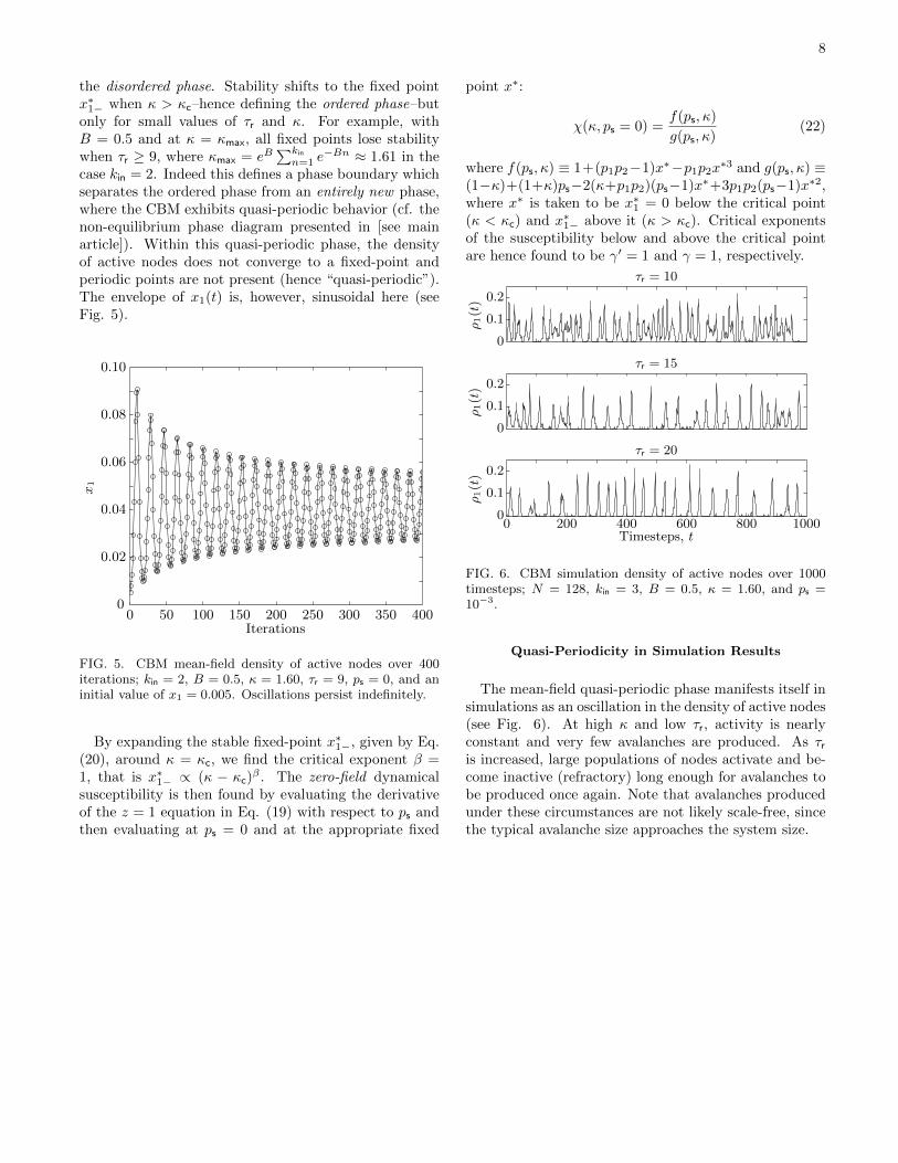
−Bn ≈ 1.61 in thecase kin = 2. Indeed this defines a phase boundary whichseparates the ordered phase from an entirely new phase,where the CBM exhibits quasi-periodic behavior (cf. thenon-equilibrium phase diagram presented in [see mainarticle]). Within this quasi-periodic phase, the densityof active nodes does not converge to a fixed-point andperiodic points are not present (hence “quasi-periodic”).The envelope of x1(t) is, however, sinusoidal here (seeFig. 5). 1

Iterations

x1

0 50 100 150 200 250 300 350 4000

0.02

0.04

0.06

0.08

0.10

FIG. 5. CBM mean-field density of active nodes over 400iterations; kin = 2, B = 0.5, κ = 1.60, τr = 9, ps = 0, and aninitial value of x1 = 0.005. Oscillations persist indefinitely.

By expanding the stable fixed-point x∗1−, given by Eq.(20), around κ = κc, we find the critical exponent β =1, that is x∗1− ∝ (κ − κc)

β . The zero-field dynamicalsusceptibility is then found by evaluating the derivativeof the z = 1 equation in Eq. (19) with respect to ps andthen evaluating at ps = 0 and at the appropriate fixed

point x∗:

χ(κ, ps = 0) =f(ps, κ)

g(ps, κ)(22)

where f(ps, κ) ≡ 1+(p1p2−1)x∗−p1p2x∗3 and g(ps, κ) ≡

(1−κ)+(1+κ)ps−2(κ+p1p2)(ps−1)x∗+3p1p2(ps−1)x∗2,where x∗ is taken to be x∗1 = 0 below the critical point(κ < κc) and x∗1− above it (κ > κc). Critical exponentsof the susceptibility below and above the critical pointare hence found to be γ′ = 1 and γ = 1, respectively.

1

τr = 10

ρ1(t)

0

0.1

0.2

τr = 15

ρ1(t)

0

0.1

0.2

τr = 20

Timesteps, t

ρ1(t)

0 200 400 600 800 10000

0.1

0.2

FIG. 6. CBM simulation density of active nodes over 1000timesteps; N = 128, kin = 3, B = 0.5, κ = 1.60, and ps =10−3.

Quasi-Periodicity in Simulation Results

The mean-field quasi-periodic phase manifests itself insimulations as an oscillation in the density of active nodes(see Fig. 6). At high κ and low τr, activity is nearlyconstant and very few avalanches are produced. As τris increased, large populations of nodes activate and be-come inactive (refractory) long enough for avalanches tobe produced once again. Note that avalanches producedunder these circumstances are not likely scale-free, sincethe typical avalanche size approaches the system size.