Understanding nonequilibrium scaling laws governing ...

Eur. Phys. J. B (2020) 93: 142https://doi.org/10.1140/epjb/e2020-100481-9 THE EUROPEAN

PHYSICAL JOURNAL BColloquium

Understanding nonequilibrium scaling laws governing collapseof a polymer

Suman Majumdera, Henrik Christiansenb, and Wolfhard Jankec

Institut fur Theoretische Physik, Universitat Leipzig, IPF 231101, 04081 Leipzig, Germany

Received 2 October 2019 / Received in final form 6 May 2020Published online 3 August 2020c© The Author(s) 2020. This article is published with open access at Springerlink.com

Abstract. Recent emerging interest in experiments of single-polymer dynamics urge computational physi-cists to revive their understandings, particularly in the nonequilibrium context. Here we briefly discussthe currently evolving approaches of investigating the evolution dynamics of homopolymer collapse usingcomputer simulations. Primary focus of these approaches is to understand various dynamical scaling lawsrelated to coarsening and aging during the collapse in space dimension d = 3, using tools popular innonequilibrium coarsening dynamics of particle or spin systems. In addition to providing an overview ofthose results, we also present new preliminary data for d = 2.

1 Introduction

Understanding various scaling laws governing a phasetransition has been one of the primary research topics overthe last fifty years, be it from an equilibrium perspectiveor at the nonequilibrium front [1–4]. Also for polymers, theequilibrium aspects of phase transitions have been stud-ied extensively [5–8]. Polymers in general represent a largeclass of macromolecules be they chemically synthesized ornaturally occurring. A range of fundamentally importantbiomolecules, e.g., proteins and DNA, fall under the broadcanopy of polymers. Most of these polymeric systemsexhibit some form of conformational phase transitionsdepending on certain external conditions, viz., the collapsetransition in homopolymers. Upon changing the solventcondition from good (where monomer-solvent interactionis dominating). to poor (where monomer-monomer inter-action is stronger), a homopolymer undergoes a collapsetransition from its extended coil state to a compact glob-ule [9,10]. This transition belongs to a class of phasetransitions that can be understood by investigating var-ious associated scaling laws [5–8]. From a general pointof view, the understanding of the collapse transition inhomopolymers can be extended to investigate other con-formational transitions experienced by different types ofmacromolecules, e.g., in a protein the collapse of the back-bone may occur simultaneously or precede its folding to anative state [11–15].

Due to certain technical difficulties such as prepar-ing a super-dilute solution or finding a long enough

a e-mail: [email protected] e-mail: [email protected] e-mail: [email protected]

polymer with negligible polydispersity, the experimen-tal realization of the collapse transition was rare in thepast [10,16]. Since the introduction of technical equipmentlike small angle X-ray scattering, single molecule fluores-cence, dynamic light scattering, dielectric spectroscopy,etc., monitoring the behaviour of a single macromoleculehas become feasible [17–19]. On the other hand, theo-retically the scaling laws related to the static and theequilibrium dynamic aspects of the transition are wellunderstood since a long time [5–8].

In contrast to the equilibrium literature, however, in thenonequilibrium aspects, i.e., for the kinetics of the collapsetransition, there is no unanimous theoretical understand-ing even though quite a few analytical and computationalstudies have been conducted [20–35]. The aforesaid exper-imental developments to track single polymers and thelack of understanding of the nonequilibrium dynamicsof polymers motivated us to perform a series of workson the kinetics of polymer collapse [36–41]. There ournovel approach of understanding the collapse by using itsanalogy with usual coarsening phenomena of particle andspin systems provided intriguing new insights, as will bediscussed subsequently.

Most of the studies on collapse kinetics in the pastdealt with the understanding of the relaxation time, i.e.,the time a system requires to attain its new equilibriumstate once its current state is perturbed by a suddenchange of the environmental conditions, e.g., the temper-ature. In the context of polymer collapse, the relaxationtime is referred to as the collapse time τc, which mea-sures the time a polymer that is initially in an extendedstate needs to reach its collapsed globular phase. Obvi-ously, τc depends on the degree of polymerization or chainlength N of the polymer (the number of repeating units

https://epjb.epj.org/

https://doi.org/10.1140/epjb/e2020-100481-9

http://www.springerlink.com

mailto:[email protected]



Page 2 of 19 Eur. Phys. J. B (2020) 93: 142

or monomers in the chain), which can be described by thescaling relation

τc ∼ Nz, (1)

where z is the corresponding dynamical exponent. Theabove relation is reminiscent of the scaling one observesfor dynamic critical phenomena [42]. The other impor-tant aspect of the kinetics is the growth of clusters ofmonomers that are formed during the collapse [21,31]. Thecluster growth has recently been understood by us usingthe phenomenological similarities of collapse with coarsen-ing phenomena in general [36,39,40]. Moreover, along thesame line one can also find evidence of aging and relatedscaling laws [37–40] that was mostly ignored in the past.

In this Colloquium, we intend to give a brief reviewof the results available on collapse kinetics based onthe above mentioned three topics: relaxation, coarsen-ing, and aging. It is organized in the following way. Wewill begin with an overview of the phenomenological the-ories of collapse dynamics followed by an overview ofthe previous simulation results in Section 2. Afterwards,in Section 3, we will discuss our recent developmentsconcerning the understanding of relaxation time, clustergrowth and aging for the kinetics of the collapse transi-tion in a homopolymer. Then we will present in Section 4some preliminary results on the special case of polymercollapse kinetics in space dimension d = 2. In Section 5,finally, we wrap up with a discussion and an outlook tofuture research in this direction.

2 Overview of previous studies on collapsedynamics

The first work on the collapse dynamics dates back to 1985when de Gennes proposed the phenomenological sausagemodel [20]. It states that the collapse of a homopolymerproceeds via the formation of a sausage-like intermediatestructure which eventually minimizes its surface energythrough hydrodynamic dissipation and finally forms acompact globule having a spherical shape. Guided by thispicture, in the next decade there was a series of numericalworks by Dawson and co-workers considering both lat-tice and off-lattice models [21–26]. However, the sequenceof events obtained in their simulations differs substan-tially from the sausage model. Later in 2000, Halperin andGoldbart (HG) came up with their pearl-necklace pictureof the collapse [29], consistent not only with the obser-vations of Dawson and co-workers but also with all thelater simulation results. According to HG the collapse ofa polymer upon quenching from an extended coil stateinto the globular phase occurs in three different stages: (i)initial stage of formation of many small nascent clusters ofmonomers out of the density fluctuations along the chain,(ii) growth and coarsening of the clusters by withdraw-ing monomers from the bridges connecting the clustersuntil they coalesce with each other to form bigger clustersand eventually ending up with a single cluster, and (iii)the final stage of rearrangements of the monomers withinthe single cluster to form a compact globule. Even before

the pearl-necklace picture of collapse by HG, Klushin [28]independently proposed a phenomenology for the samepicture based on similar coarsening of local clusters. Itdiffers from the HG one as it does not consider the initialstage of formation of the local ordering or small nascentclusters. However, almost all the simulation results so farhave shown evidence for the initial stage of nascent clusterformation.

In addition to the above description, HG also providedtime scales for each of these stages which scale with thenumber of monomers as N0, N1/5 and N6/5, respectively.Quite obviously this scaling of the collapse time is depen-dent on the underlying dynamics of the system, i.e., on theconsideration of hydrodynamic effects. Klushin derivedthat the collapse time τc scales as τc ∼ N1.6 in absenceof hydrodynamics whereas the collapse is much faster inpresence of hydrodynamics with the scaling τc ∼ N0.93

[28]. Similar conclusions were drawn in other theoreticaland simulation studies as well. In the following Section 2.1we discuss some of these numerical results on the scalingof the collapse time.

2.1 Earlier results on scaling of collapse time

As mentioned the dynamical exponent z in equation (1)depends on the intrinsic dynamics of the system. It isthus important to notice the method and even the typeof model one uses for the computer simulations. Theavailable results can be divided into three categories: (i)Monte Carlo (MC) and Langevin simulations with implicitsolvent effect, (ii) molecular dynamics (MD) simulationswith implicit solvent effect, and (iii) MD simulations withexplicit solvent effect. Results from MC and Langevinsimulations do not incorporate hydrodynamics and henceonly mimic diffusive dynamics. On the other hand, MDsimulations with implicit solvent, depending on the natureof the thermostat used for controlling the temperature,can be with or without hydrodynamic effects. At thispoint we caution the reader that there is a subtle dif-ference between solvent effects and hydrodynamic effects.Thus doing MD simulations with explicit solvent doesnot necessarily mean that the hydrodynamic modes areactively taken into account. Rather this depends on howone treats the momenta of the solvent particles in the sim-ulation, e.g., it depends on the choice of thermostat used[43]. This gets not only reflected in the nonequilibriumrelaxation times like the collapse time τc but also in theequilibrium autocorrelation time τ . The few existing stud-ies on polymer collapse using MD simulations that accountfor solvent effects by considering explicit solvent beads,thus, can also be classified on the basis of consideration ofhydrodynamic effects. Since there is no available appro-priate theory for the nonequilibrium relaxation time, thetrend is to compare the scaling of the collapse time withthe available theories of equilibrium polymer dynamics.In absence of hydrodynamic effects the dynamics is com-pared with Rouse scaling that states that in equilibriumthe diffusion coefficient D scales with the chain length Nas D ∼ N−1, which implies that the relaxation time scalesas τ ∼ N2 [44]. On the other hand, in presence of hydrody-namics when the polymer moves as a whole due to the flow


Eur. Phys. J. B (2020) 93: 142 Page 3 of 19

Table 1. Summary of simulation results for the scaling of the collapse time τc with the length of the polymer N asdescribed in equation (1).

Authors Model Method Explicit Solvent Hydrodynamics z

Byrne et al. (1995) [21] Off-lattice Langevin No No 3/2Kuznetsov et al. (1995) [23] Lattice MC simulations No No 2Kuznetsov et al. (1996) [24] GSC equations Numerically No No 2Kuznetsov et al. (1996) [24] GSC equations Numerically No Yes 3/2Kikuchi et al. (2005) [33] Off-lattice MD simulations Yes No 1.89(9)Kikuchi et al. (2005) [33] Off-lattice MD simulations Yes Yes 1.40(8)Pham et al. (2008) [34] Off-lattice BD simulations No No 1.35(1)Pham et al. (2008) [34] Off-lattice BD simulations No Yes 1.01(1)Guo et al. (2011) [35] Off-lattice DPD simulations Yes Yes 0.98(9)Majumder et al. (2017) [39] Off-lattice MC simulations No No 1.79(6)Christiansen et al. (2017) [40] Lattice MC simulations No No 1.61(5)

MC: Monte Carlo, MD: molecular dynamics, BD: Brownian dynamics, DPD: dissipative particle dynamics.

field, the corresponding scaling laws are D ∼ N−0.588 andτ ∼ N1.76, known as the Zimm scaling [45]. Both Rouseand Zimm scalings have been verified in a number of com-putational studies as well as in experiments. However, westress that the nonequilibrium relaxation time, e.g., thecollapse time τc does not necessary follow the same scalingas the equilibrium autocorrelation time τ [46,47].

In Table 1 we have summarized some of the relevantresults on the scaling of the collapse time that one canfind in the literature. In the early days the simulationswere done mostly by using methods that do not incor-porate hydrodynamics, e.g., numerical solution of theGaussian-self consistent (GSC) equations, MC simula-tions and Langevin simulations. They considered modelswhich could be either on-lattice (interacting self-avoidingwalks) or off-lattice (with Lennard-Jones kind of inter-action). The GSC approach and MC simulations (in alattice model) provided z that matches with the Rousescaling in equilibrium [23,24]. Langevin simulations of anoff-lattice model yielded z ≈ 3/2 [21] which was the valuelater obtained in a theory by Abrams et al. [31]. Kikuchiet al. [30] went a step further by doing MD simulations ofan off-lattice model with explicit solvent which also allowsone to tune the hydrodynamic interactions. In absence ofhydrodynamics they obtained values of z ≈ 1.9 close to theRouse value of 2 [33]. On the other hand, in presence ofhydrodynamics the dynamics is much faster with z ≈ 1.4[33]. This is more or less in agreement with GSC resultsobtained considering hydrodynamic interaction [24]. Latermore simulations on polymer collapse with explicit solventwere performed. In this regard, relatively recent Browniandynamics (BD) simulations with explicit solvent (hydro-dynamic interaction preserved) by Pham et al. providedeven faster dynamics with z ≈ 1 [34]. There exist evennewer results from dissipative-particle dynamics (DPD)simulation that also reports z ≈ 1 [35]. Note that theseresults do not well compare with the Zimm scaling applica-ble to equilibrium dynamics in presence of hydrodynamics.The bottom line from this literature survey is that noconsensus has been achieved for the value of z. In ourrecent results on collapse dynamics from MC simulationsa consistent value of z was obtained between an off-latticemodel and a lattice model with z ≈ 1.7 [39,40].

2.2 Earlier results on cluster growth

As discussed above most of the previous studies onkinetics of the collapse transition focused on understand-ing the scaling of the collapse time. However, going bythe phenomenological picture described by HG, as alsoobserved in most of the available simulation results, thesecond stage of the collapse, i.e., the coalescence of the“pearl-like” clusters to form bigger clusters and therebyeventually a single globule bears resemblance to usualcoarsening of particle or spin systems. The nonequilibriumphenomenon of coarsening in particle or spin systems iswell understood [4,48] with current focus shifting towardsmore challenging scenarios like fluid mixtures [49,50]. Fun-damentally, too, it is still developing as for example incomputationally expensive long-range systems [51–53].

In usual coarsening phenomena, e.g., in ordering offerromagnets after quenching from the high-temperaturedisordered phase to a temperature below the critical point,the nonequilibrium pathway is described by a growinglength scale, i.e., average linear size of the domains `(t)as [4,48]

`(t) ∼ tα. (2)

The value of the growth exponent α depends on the con-cerned system as well as the conservation of the orderparameter during the entire process. For example, in solidbinary mixtures where the dynamics is conserved, α = 1/3which is the Lifshitz-Slyozov (LS) growth exponent [54],whereas for a ferromagnetic ordering where the orderparameter is not conserved, α = 1/2 which is referred to asthe Lifshitz-Cahn-Allen (LCA) growth [55]. On the otherhand, in fluids where in simulations one must incorporatehydrodynamics, three different regimes are observed; theearly-time diffusive growth where α = 1/3 as in solids; theintermediate viscous hydrodynamic growth with α = 1[56]; and at a very late stage the inertial growth withα = 2/3 [57].

In the context of polymer collapse, the concerned grow-ing length scale could be the linear size (or radius) of theclusters. However, in all the previous works it was cho-sen to be the average mass Cs(t), or average number of



monomers present in a cluster. In spatial dimension d, itis related to the linear size of the cluster as Cs(t) ∼ `(t)d.Thus in analogy with the power-law scaling (2) of thelength scale during coarsening, the corresponding scalingof the cluster growth can then be written as

Cs(t) ∼ tαc , (3)

where αc = dα is the corresponding growth exponent.Like the dynamical exponent z, the growth exponent αcis also dependent on the intrinsic dynamics of the sys-tem. Previous studies based on MC simulations of a latticepolymer model reported αc = 1/2 [23] and Langevin simu-lations of an off-lattice model reported αc = 2/3 [21], bothbeing much smaller than αc = 1 as observed for coarseningwith only diffusive dynamics. BD simulations with explicitsolvent also provided αc ≈ 2/3 in absence of hydrodynam-ics. Like in coarsening of fluids, the dynamics of clustergrowth during collapse, too, gets faster when hydrody-namic effects are present. For instance, BD and DPDsimulations with incorporation of hydrodynamic effectsyield αc ≈ 1 [34,35]. Surprisingly, our recent result on anoff-lattice model via MC simulations also showed αc ≈ 1[39]. This will be discussed in Section 3.4.

2.3 Earlier results on aging during collapse

Apart from the scaling of the growth of the averagedomain size during a coarsening process there is anotherimportant aspect, namely, aging [58,59]. The fact that ayounger system relaxes faster than an older one forms thefoundation of aging in general. This is also an essentialconcept from the point of view of glassy dynamics [60,61].Generally, aging is probed by the autocorrelation functionof a local observable Oi given as

C(t, tw) = 〈Oi(t)Oi(tw)〉 − 〈Oi(t)〉〈Oi(tw)〉, (4)

with t and tw < t being the observation and the wait-ing time, respectively. The 〈. . . 〉 denotes averaging overseveral randomly chosen realizations of the initial config-uration and independent time evolutions. The observableOi is generally chosen in such a way that it clearly reflectsthe changes happening during the concerned nonequilib-rium process, e.g., the time- and space-dependent orderparameter during ferromagnetic ordering.

There are three necessary conditions for aging: (i)absence of time-translation invariance in C(t, tw), (ii) slowrelaxation, i.e., the relaxation times obtained from thedecay of C(t, tw) should increase as function of tw, and(iii) the observation of dynamical scaling of the form

C(t, tw) ∼ x−λc ; xc = `/`w (5)

where ` and `w are the characteristic length scales attime t and tw, respectively, and λ is the correspondingautocorrelation exponent. For the choice xc = t/tw, thecorresponding autocorrelation exponent is αλ where thegrowth exponent α relates ` and t [see Eq. (2)]. Fisher andHuse (FH) in their study of ordering spin glasses proposed

a bound on λ which only depends on the dimension d as[62]

d

2≤ λ ≤ d. (6)

Later this bound was found to be obeyed in the ferromag-netic ordering as well [63–65]. An even stricter and moregeneral bound was later proposed by Yeung et al. [66]that also includes the case of conserved order-parameterdynamics.

In the context of polymer collapse, although analo-gous to coarsening phenomena in general, this particularaspect of aging has received very rare attention [67,68].There, like in other soft-matter systems [69–71] the resultsindicated presence of subaging, i.e., evidence for scalingsimilar to equation (5) but as a function of xc = t/tµwwith µ < 1. Afterwards, there were no attempts to quan-tify this scaling with respect to the ratio of the growinglength scale. In our approach, both with off-lattice andlattice models we showed that simple aging scaling as inequation (5) with respect to the ratio of the cluster sizescan be observed [37–40]. Thus to quantify the aging scal-ing, by choosing xc = Cs(t)/Cs(tw) one has to transformequation (5) to

C(t, tw) ∼[Cs(t)

Cs(tw)

]−λc

(7)

where λc is the associated autocorrelation exponent whichis related to the traditional exponent λ via the relationλc = λ/d.

3 Recent Monte Carlo results in d = 3

In this section we will review the very recent developmentsby us concerning the kinetics of homopolymer collapsefrom all above mentioned three perspectives. We will com-pare the results from an off-lattice model (OLM) anda lattice model (LM), focusing in this section on d = 3dimensions. New results for the special case of d = 2 willbe presented in the next section to check the validity ofthe observations in general. Before moving on to a dis-cussion of our findings next we first briefly describe thedifferent models and methodologies used in our studies.

3.1 Models and methods

For OLM, we consider a flexible bead-spring model wherethe connectivity between two successive monomers orbeads is maintained via the standard finitely extensiblenon-linear elastic (FENE) potential

EFENE(rii+1) = −K2R2 ln

[1−

(rii+1 − r0

R

)2]. (8)

We chose the force constant of the spring K = 40, themean bond length r0 = 0.7 and the maximum alloweddeviation from the mean position R = 0.3 [72]. Monomers



were considered to be spherical beads with diameterσ = r0/2

1/6. The nonbonded interaction between themonomers is given by

Enb(rij) = ELJ (min[rij , rc])− ELJ(rc), (9)

where

ELJ(r) = 4ε

[(σr

)12−(σr

)6](10)

is the standard Lennard-Jones (LJ) potential. Here ε (= 1)is the interaction strength and rc = 2.5σ the cut-off radius.

For LM, we consider a variant of the interactive self-avoiding walk on a simple-cubic lattice, where each latticesite can be occupied by a single monomer. The Hamilto-nian is given by

H = −1

2

∑i6=j,j±1

w(rij), where w(rij) =

{J rij = 1

0 else.

(11)Here rij is the distance between two nonbonded monomersi and j, w(rij) is an interaction parameter that considersonly nearest neighbours, and J (= 1) is the interactionstrength. We allowed a fluctuation in the bond length byconsidering diagonal bonds, i.e., the possible bond lengthsare 1,

√2 and

√3. The model has been independently

studied for equilibrium properties [73,74]. It has certainsimilarities with the bond-fluctuation model [75]. For acomparison between them, please see reference [76].

The dynamics in the models can be introduced viaMarkov chain MC simulations [46,77], however, with therestriction of allowing only local moves. For OLM thelocal moves correspond to shifts of a randomly selectedmonomer to a new position randomly chosen within[−σ/10 : σ/10] of its current position. For LM, too, themove set consists of just shifting a randomly chosenmonomer to another lattice site such that the bond con-nectivity constraint is maintained. These moves are thenaccepted or rejected following the Metropolis algorithmwith Boltzmann criterion [46,77]. The time scale of thesimulations is one MC sweep (MCS) which consists of N(where N is the number of monomers in the chain) suchattempted moves.

The collapse transition temperature is Tθ(N → ∞)≈ 2.65 ε/kB and ≈ 4.0 J/kB for OLM and LM, respec-tively [39,40]. In all the subsequent discussion, the unitof temperature will always be ε/kB or J/kB with theBoltzmann constant kB being set to unity. Following thestandard protocol of nonequilibrium studies we first pre-pared initial conformations of the polymers at high tem-perature Th ≈ 1.5Tθ that mimics an extended coil phase.Then this high-temperature conformation was quenchedto a temperature Tq < Tθ. Since LM is computationallyless expensive than OLM, the chain length of polymerused for LM is longer than what is used for OLM. Notethat except for the evolution snapshots, for both mod-els, all the results presented were obtained after averagingover more than 300 independent runs. For each such run,the starting conformation is an extended coil which were

obtained independently of each other by generating self-avoiding walks using different random seeds and thenequilibrating them at the high temperature Th.

3.2 Phenomenological picture of the collapse

As mentioned before even though the sausage pictureof de Gennes [20] is the pioneer in describing the phe-nomenology of the collapse dynamics, all simulation stud-ies provided evidence in support of the pearl-necklacepicture of HG [29]. In our simulations, too, both withOLM and LM, we observed intermediates that support thepearl-necklace phenomenology. Typical snapshots whichwe obtained from our simulations are shown in Figure 1.The sequence of events happening during the collapse iscaptured by these snapshots. At initial time the poly-mer is in an extended state with fluctuations of the localmonomer density along the chain. Soon there appear anumber of local clusters of monomers which then startto grow by withdrawing monomers from the rest of thechain. This gives rise to the formation of the so calledpearl-necklace. Once the tension in the chain is at maxi-mum, two successive clusters along the chain coalesce witheach other to grow in size. This process goes on untila single cluster or globule is formed. The final stage ofthe collapse is the rearrangement of the monomers withinthe single cluster to form a compact globule. This laststage, however, is difficult to disentangle from the previousstages.

The first two stages of formation and growth of clus-ters during the collapse of a polymer as demonstrated inFigure 1 are clearly reminiscent of usual coarsening phe-nomena in particle or spin systems. As already mentionedtraditionally for studying coarsening one starts with aninitial state where the distribution of particles or spinsis homogeneous, e.g., homogeneous fluid or paramagnetabove the critical temperature. Similarly to study the col-lapse kinetics one starts with a polymer in the extendedcoil phase which is analogous to the homogeneous phase inparticle or spin systems. Usual coarsening sets in when theinitial homogeneous configuration is suddenly cooled downto a temperature below the critical temperature wherethe equilibrium state is an ordered state, e.g., condenseddroplet in fluid background or ferromagnet. Similarly, fora polymer, the collapse occurs when the temperature issuddenly brought down below the corresponding collapsetransition temperature. There the equilibrium collapsedphase is analogous to the droplet phase in fluids.

Now coarsening refers to the process via which the ini-tial homogeneous system evolves while approaching theordered phase. This happens via the formation and sub-sequent growth of domains of like particles or spins. Thisis illustrated in the upper panel of Figure 2 where weshow the time evolution of the droplet formation in afluid starting from a homogeneous phase via MC sim-ulations of the Ising lattice gas. At early times manysmall domains or droplets are formed which then coarsento form bigger droplets and eventually giving rise to asingle domain or droplet. A similar sequence of eventsis observed during collapse of a polymer as shown onceagain in the lower panel of Figure 2 which explains the



Fig. 1. Time-evolution snapshots during collapse of a homopolymer showing pearl-necklace formation, following a quench froman extended coil phase to a temperature, Tq = 1 for OLM and Tq = 2.5 for LM, in the globular phase. The chain lengths Nused are 724 and 4096 for OLM and LM, respectively. Taken from reference [41].

Fig. 2. Illustration of the similarities between the collapse kinetics and the usual coarsening of a particle system. The upper panelshows evolution snapshots for the droplet formation in a particle system using the Ising lattice gas in two spatial dimensions.The lower panel shows the evolution of a homopolymer obtained from simulation of the OLM.



phenomenological analogy of collapse with usual coarsen-ing phenomena. Coarsening from a theoretical point ofview is understood as a scaling phenomenon which meansthat certain morphology-characterizing functions of thesystem at different times can be scaled onto each otherusing corresponding scaling functions [4,48]. This scalingin turn also implies that there must be scaling of the time-dependent length scale, too, which in most of the casesshows a power-law scaling like in equation (2). Based onthis understanding in general and the above mentionedanalogy we will discuss in the remaining part of thissection how to investigate the presence of nonequilibriumscaling laws in the dynamics of collapse of a homopolymer.

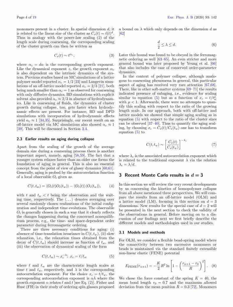
3.3 Relaxation behaviour of the collapse

In all earlier studies, the straightforward way to quantifythe kinetics was to monitor the time evolution of the over-all size of the polymer, i.e., the squared radius of gyrationgiven as

R2g =

1

N

N∑i=1

(ri − rcm)2 (12)

where rcm is the center of mass of the polymer. In thecoiled state (above Tθ), R

2g ∼ N2νF with νF = 3/5, in the

Flory mean-field approximation, whereas in the globularstate (below Tθ), R

2g ∼ N2/d is much smaller [78]. Such

decay of R2g with time is shown in Figure 3a for both

OLM and LM. Although in some of the earlier studies apower-law decay of R2

g is suggested, in most cases or atleast in the present cases that does not work. Rather, thedecay can be well described by the form

R2g(t) = b0 + b1 exp

[−(t

τf

)β], (13)

where b0 corresponds to the saturated value of R2g(t) in the

collapsed state, b1 is associated with the value at t = 0,and β and τf are fitting parameters. For details aboutfitting the data with the form (13), see references [39]and [40] for OLM and LM, respectively. An illustration ofhow appropriately this form works is shown in Figure 3a.There the respective solid lines are fits to the form (13).While the above form does not provide any detail aboutthe specificity of the collapse process, it gives a measure ofthe collapse time τc via τf . However, to avoid the unreli-able extraction of the collapse time from such a fitting, onecould alternatively use a rather direct way of estimatingτ50 which corresponds to the time when R2

g(t) has decayed

to half of its total decay, i.e.,[R2g(0)−R2

g(∞)]/2. Data

for both models as shown in Figure 3b reflect a power-lawscaling, to be quantified with the form

τc = BNz + τ0, (14)

where B is a nontrivial constant that depends on thequench temperature Tq, z is the corresponding dynamical

Fig. 3. (a) Time dependence of the squared radius of gyra-tion, R2

g(t), for both OLM (Tq = 1.0) and LM (Tq = 2.5).The solid lines are fits to the data using the form describedby equation (13) with β = 1.18 and 1.15 for OLM and LM,respectively. (b) Scaling of the collapse time, τ50, with respectto N . The solid lines are fits to the form (14). The dashed lineis a fit of the OLM data for N ≥ 128, to the form (14) by fixingz = 1. Adapted from reference [41].

exponent, and the offset τ0 comes from finite-size correc-tions. For LM a fitting (shown by the corresponding solidline) with the form (14) provides z = 1.61(5) and is almostinsensitive to the chosen range. However, for OLM the fit-ting is sensitive to the chosen range. While using the wholerange of data provides z = 1.80(6) (shown by the corre-sponding solid line), fitting only the data for N ≥ 128yields z = 1.20(9). In this regard, a linear fit [fixing z = 1in (14)], shown by the dashed line, also works quite well.For a comparison of the values of z obtained by us withthe ones obtained by others, see Table 1.

3.4 Coarsening during collapse

Having the phenomenological analogy between collapse ofa polymer and usual coarsening of particle and spin sys-tems established, in this subsection we present the scalingof the cluster growth during the collapse under the lightof well established protocols of the coarsening in particleor spin systems.



3.4.1 Scaling of morphology-characterizing functions

Coarsening in general is a dynamical scaling phenomenon,where certain structural quantities that quantify themorphology of the system, e.g., two-point equal-timecorrelation functions and structure factors show scalingbehaviour with time [4,48]. This means that the structurefactors at different times can be collapsed onto the samemaster curve by using the relevant length scales, i.e., clus-ter size or domain size at those times. This fact is usedto extract the relevant time-dependent length scale thatgoverns the kinetics of coarsening. For example one usesthe first moment of the structure factor at a particulartime to have a measure of the length scale or the averagedomain size during coarsening. However, to understandthe kinetics of cluster growth during the collapse of apolymer traditionally the average number of monomerspresent in a cluster is used as the relevant length scaleCs(t). For studying the OLM we used this definition tocalculate Cs(t), details of which can be found in reference[39] and later will also be discussed in Section 4.1 for thed = 2 case. The validity of this definition as the relevantlength scale can be verified by looking at the expectedscaling of the cluster-size distribution P (Cd, t), i.e., theprobability to find a cluster of size Cd among all the clus-ters at time t. Using this distribution we calculate theaverage cluster size as Cs(t) = 〈Cd〉. The correspondingscaling behaviour is given as

P (Cd, t) ≡ Cs(t)−1P [Cd/Cs(t)], (15)

where P is the scaling or master function. This means thatwhen Cs(t)P (Cd, t) at different times are plotted againstCd/Cs(t) they should fall on top of each other. This veri-fication is presented in Figure 4 where in the main framewe show plots of the (unscaled) distributions P (Cd, t) atdifferent times, and in the inset the corresponding scalingplot using the form (15). Coincidentally, here, the tail ofthe distribution shows an exponential decay as observedin coarsening of particle [79] and spin systems [80,81].

On the other hand, for a lattice model, one can usethe advantage of having the monomers placed on latticepoints. There a two-point equal-time correlation functioncan be defined as

C(r, t) = 〈ρ(0, t)ρ(r, t)〉 (16)

with

ρi(r, t) =1

mr

∑j,rij=r

θ(rj , t) (17)

where the characteristic function θ is unity if there is amonomer at position rj or zero otherwise. mr denotes thenumber of possible lattice points at distance r from anarbitrary point of the lattice. Plots for such correlationfunctions at different times during the collapse of a poly-mer using LM are shown in the main frame of Figure 5.Slower decay of C(r, t) as time increases suggests the pres-ence of a growing length scale. Thus following the trendin usual coarsening studies one can extract an average

Fig. 4. Normalized distribution of the cluster sizes at threedifferent times during the coarsening stage of the collapse atTq = 1 for a polymer with N = 724 modeled by OLM. Theinset demonstrates the scaling behaviour of the collapse phe-nomenon via the semi-log plot of the corresponding scalingof the distribution functions. The solid line shows consistencyof the data with an exponential tail. Taken from reference[39]. (@ Royal Society of Chemistry, 2017. This figure is sub-ject to copyright protection and is not covered by a CreativeCommons license.)

Fig. 5. Morphology characterizing two-point equal-time corre-lation function C(r, t) at different times, showing the presenceof a growing length scale during collapse of a polymer obtainedvia simulation of LM with Tq = 2.5 and N = 4096. The insetshows the presence of scaling in the process via a plot of thesame data as a function of r/`(t) where `(t) is the characteristiclength scale calculated using (18) with h = 0.1. Adapted fromreference [40]. (@ AIP, 2017. This figure is subject to copyrightprotection and is not covered by a Creative Commons license.)

length scale `(t) that characterizes the clustering duringthe collapse, via the criterion

C (r = `(t), t) = h, (18)



where h denotes an arbitrary but reasonably chosen valuefrom the decay of C(r, t). Calculation of `(t) in the abovemanner automatically suggests to look for the dynamicalscaling of the form

C(r, t) ≡ C (r/`(t)) , (19)

where C is the scaling function. Such a scaling behaviouris nicely demonstrated in the inset of Figure 5, where weshow the corresponding data presented in the main frameas function of r/`(t). Note that here `(t) gives the linearsize of the ordering clusters. Thus in order to compare`(t) of LM with the cluster size Cs(t) obtained for OLMone must use the relation `(t)d ≡ Cs(t). For a check of thevalidity of this relation, see reference [40].

3.4.2 Cluster growth

Once it is established that the coarsening stage of polymercollapse is indeed a scaling phenomenon, the next inter-est goes towards checking the associated growth laws. InFigure 6a, we show the time dependence of Cs(t) for OLMand LM. To make the data from both models visible onthe same scale there the y-axis is scaled by the correspond-ing chain length N of the polymer. Note that saturationof the data for LM at a value less than unity is due to thefact that there we have calculated the average cluster sizeCs(t) from the decay of the correlation function C(r, t)as described in the previous subsection. This gives a pro-portionate measure of the average number of monomerspresent in the clusters and thus the data saturate to avalue less than unity.

In coarsening kinetics of binary mixtures such timedependence of the relevant length scale can be describedcorrectly when one considers an off-set in the scalingansatz [80,82–84]. Similarly, it was later proved to beappropriate for the cluster growth during the collapse of apolymer [36,39]. Following this one writes down the scalingansatz as

Cs(t) = C0 +Atαc , (20)

where C0 corresponds to the cluster size after crossingover from the initial cluster formation stage, and A isa temperature-dependent amplitude. The solid lines inFigure 6a are fits to the form (20) yielding αc = 0.98(4)and 0.62(5) for OLM and LM, respectively.

One can verify the robustness of the growth by studyingthe dependence of cluster growth on the quench temper-ature Tq. For this one uses data at different Tq and canperform a scaling analysis based on nonequilibrium finite-size scaling (FSS) arguments [39]. The nonequilibriumFSS analysis was constructed based on FSS analyses inthe context of equilibrium critical phenomena [85,86]. Anaccount of the FSS formulation in the present context canbe found in reference [39]. In brief, one introduces in thegrowth ansatz (20) a scaling function Y (yp) as

Cs(t)− C0 = (Cmax − C0)Y (yp), (21)

Fig. 6. (a) Plots of the average cluster size Cs(t)/N , as func-tion of time for the systems presented in Figure 1. To makeboth the data visible on the same plot, we divide the timeaxis by a factor m to obtain tp = t/m, where m = 1× 106 and3.5× 106 for OLM and LM, respectively. The solid lines are fitsto the form (20) with αc = 0.98 for OLM and αc = 0.62 forLM. The plots in (b) and (c) demonstrate the scaling exercisefor OLM with αc = 1.0 and LM with αc = 0.62, respectively,showing that data for Cs(t) at different quench temperaturesTq can be collapsed onto a master curve using a nonuniversalmetric factor in the scaling variable. The solid lines repre-sent the corresponding Y (yp) ∼ y−αc

p behaviour. Adapted fromreference [41].

which implies

Y (yp) =Cs(t)− C0

Cmax − C0, (22)

where Cmax ∼ N is the maximum cluster size a finite sys-tem can attain. In order to account for the temperature-dependent amplitude A(Tq), one uses the scaling variable

yp = fs(N − C0)1/αc

t− t0(23)



where

fs =

[A(Tq,0)

A(Tq)

]1/αc

. (24)

The metric factor fs is introduced for adjusting thenonuniversal amplitudes A(Tq) at different Tq. Here, inaddition to C0 one also uses the crossover time t0 fromthe initial cluster formation stage. A discussion of the esti-mation of C0 and t0 can be found in references [39,40].While performing the exercise we tune the parameters αcand fs to obtain a data collapse along with the Y (yp)∼ y−αc

p behaviour in the finite-size unaffected region. InFigures 6b and 6c, we demonstrate such scaling exerciseswith αc = 1.0 and 0.62 for OLM and LM, respectively.For fs, we use the reference temperature Tq,0 = 1.0 and2.0 for OLM and LM, respectively. The collapse of datafor different Tq and consistency with the correspondingy−αcp behaviour in both plots suggest that the growth is

indeed quite robust and can be described by a single uni-versal FSS function with nonuniversal metric factor fs inthe scaling variable. However, αc in OLM is larger than forLM, a fact in concurrence with the values of z estimatedpreviously, and thus to some extent providing support tothe heuristic relation z ∼ 1/αc. The use of a nonuniver-sal metric factor in order to find a universal FSS functionwas first introduced in the context of equilibrium criti-cal phenomena using different lattice types [87,88]. Afteradapting this concept to nonequilibrium FSS of polymerkinetics in references [39,40] as explained above, it wasrecently also transferred to spin systems where its useful-ness has been demonstrated in a coarsening study of thePotts model with conserved dynamics [81].

3.5 Aging and related scaling

Apart from the scaling of the growing length scale or thecluster size that deals only with equal-time quantities,coarsening processes are associated with the aging phe-nomenon as well. Thus along the same line, in order tocheck aging during collapse of a polymer one can calcu-late the two-time correlation or autocorrelation functiondescribed in equation (4). However, unlike for spin sys-tems here the choice of the observable Oi is not trivial.Nevertheless, for OLM we identified the observable Oi asa variable based on the cluster identification method. Weassign Oi = ±1 depending on whether the monomer isinside (+1) or outside (−1) a cluster. It is apparent thatour cluster identification method is based on the local den-sity around a monomer along the chain. Thus C(t, tw)calculated using this framework gives an analogue of theusual density-density autocorrelation function in particlesystems. On the other hand for LM, we assign Oi = ±1 bychecking the radius r at which the local density, given byρi(r, t) [see Eqs. (16) and (17)], first falls below a threshold

of 0.1. If this radius is smaller than√

3 we assign Oi = 1,marking a high local density, otherwise we chose Oi = −1to mark a low local density. For details see references [39]and [40] for OLM and LM, respectively.

Fig. 7. Demonstration of aging phenomenon during collapseof a polymer for (a) OLM (N = 724, Tq = 1.0) and (b)LM (N = 8192, Tq = 1.5). The main frames show plots ofthe autocorrelation functions calculated using (4) at differentwaiting times tw, as mentioned there. The insets show the cor-responding scaling plots with respect to the scaling variablexc = Cs(t)/Cs(tw), in accordance with (7). The solid linesdepict the consistency of the data with a power law havingan exponent λc = 1.25. The plots in (a) and (b) are adaptedfrom references [39] and [40], respectively. (Panels (a) and (b)are subject to copyright protection and are not covered by aCreative Commons license.)

In the main frames of Figures 7a and 7b we show plotsof the autocorrelation function C(t, tw) against the trans-lated time t − tw for (a) OLM and (b) LM. Data fromboth the cases clearly show breaking of time-translationinvariance, one of the necessary conditions for aging. It isalso evident that as tw increases, the curves decay moreslowly, an indication of slow relaxation behaviour fulfill-ing the second necessary condition for aging. As a checkof the final condition for aging, i.e., dynamical scaling, inprinciple one could study the scaling with respect to thescaled time t/tw. Although such an exercise provides areasonable collapse of data for OLM, data for LM do notshow scaling with respect to t/tw. In this regard, one couldlook for special aging behaviour that can be achieved by



considering [58]

C(t, tw) ≡ G(h(t)

h(tw)

), (25)

with the scaling variable

h(t) = exp

(t1−µ − 1

1− µ

). (26)

Here, G is the scaling function and µ is a nontrivialexponent. Special aging with 0 < µ < 1 is referred toas subaging and has been observed mostly in soft-mattersystems [69–71], in spin glasses [89–91], and recently inlong-range interacting systems [92]. The µ > 1 case isreferred to as superaging and was claimed to be observedin site-diluted Ising ferromagnets. However, Kurchan’slemma [93] rules out the presence of apparent superaging[94]. This was further consolidated via numerical evidencein reference [95]. There it has been argued that the truescaling is observed in terms of the ratio of growing lengthscales at the corresponding times, i.e., `(t)/`(tw). In thecase of polymer collapse with LM, too, one apparentlyobserves special scaling of the form (25) with µ < 1, i.e.,subaging in this case. However, following the argumentof Park and Pleimling [95], one gets also here the sim-ple scaling behaviour with respect to the scaling variablexc = Cs(t)/Cs(tw), thus ruling out the presence of sub-aging. Such scaling plots of the autocorrelation data bothfor OLM and LM are shown in the insets of Figure 7. Inboth cases the data seem to follow the power-law scalingwith a decay exponent λc ≈ 1.25.

Relying on the fact that the calculation of C(t, tw) isbased on the cluster identification criterion, i.e., by calcu-lating the local monomer densities around each monomeralong the polymer chain, it gives an analogue to the usualdensity-density autocorrelation function as used in glassysystems. Keeping in mind the corresponding argument forthe bounds on the respective autocorrelation exponentfor spin-glass and ferromagnetic ordering, one can thusassume [37] C(t, tw) ∼ 〈ρ(t)ρ(tw)〉 where ρ is the averagelocal density of monomers. Now let us consider a set of Csmonomers at t (�tw) and assume that at tw the polymeris more or less in an extended coil state where the squaredradius of gyration scales as R2

g ∼ N2νF . Using Cs ≡ N inthis case one can write

ρ(tw) ∼ Cs/Rgd ∼ C−(νF d−1)s . (27)

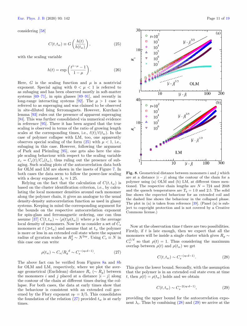
The above fact can be verified from Figures 8a and 8bfor OLM and LM, respectively, where we plot the aver-age geometrical (Euclidean) distance Re (∼ Rg) betweenthe monomers i and j placed at a distance |i − j| alongthe contour of the chain at different times during the col-lapse. For both cases, the data at early times show thatthe behaviour is consistent with an extended coil gov-erned by the Flory exponent νF = 3/5. This consolidatesthe foundation of the relation (27) provided tw is at earlytimes.

Fig. 8. Geometrical distance between monomers i and j whichare at a distance |i − j| along the contour of the chain for apolymer using (a) OLM and (b) LM, at different times men-tioned. The respective chain lengths are N = 724 and 2048and the quench temperatures are Tq = 1.0 and 2.5. The solidline shows the expected behaviour for an extended coil andthe dashed line shows the behaviour in the collapsed phase.The plot in (a) is taken from reference [39]. (Panel (a) is sub-ject to copyright protection and is not covered by a CreativeCommons license.)

Now at the observation time t there are two possibilities.Firstly, if t is late enough, then we expect that all themonomers will be inside a single cluster which gives Rg ∼C

1/ds so that ρ(t) = 1. Thus considering the maximum

overlap between ρ(t) and ρ(tw) we get

C(t, tw) ∼ C−(νF d−1)s . (28)

This gives the lower bound. Secondly, with the assumptionthat the polymer is in an extended coil state even at timet, then ρ(t) = ρ(tw) holds and we obtain

C(t, tw) ∼ C−2(νF d−1)s , (29)

providing the upper bound for the autocorrelation expo-nent λc. Thus by combining (28) and (29) we arrive at the



bounds [37]

(νF d− 1) ≤ λc ≤ 2(νF d− 1). (30)

Putting νF = 3/5 in (30) one would get 4/5 ≤ λc ≤ 8/5.Further, inserting the more precise numerical estimate ind = 3 as [96,97] νF = 0.587 597, we get

0.762 791 ≤ λc ≤ 1.525 582. (31)

The validity of this bound can also be readily verifiedfrom the consistency of our data in the insets of Figure 7with the solid lines having a power-law decay with expo-nent 1.25. We make the choice of tw in all the plots sothat the assumption that at time tw the polymer is in anextended coil state is valid. This choice can also be appre-ciated from the plots in Figures 8a and 8b for OLM andLM, respectively. There it is evident that the extendedcoil behaviour (Re ∼ |i − j|3/5) at early times is gradu-ally changing to the behaviour expected for the collapsedphase (Re ∼ |i− j|1/d with d = 3) at late times. The lit-tle off behaviour of the data for higher tw in the inset ofFigure 7 is indeed due to the fact that at those times theformation of stable clusters has already initiated to changethe extended coil behaviour of the chain. Confirmation ofthe value of λc via FSS can also be done as presented inreferences [37,40].

To confirm the robustness of the above bound and thevalue of λc, we plot C(t, tw) from different temperaturesTq in Figure 9a for OLM and Figure 9b for LM. Mereplotting of those data yields curves that are parallel toeach other due to different amplitudes. However, if oneuses a multiplier f on the y-axis to adjust those differ-ent amplitudes for different Tq one obtains curves thatfall on top of each other as shown. The values of f usedfor different Tq are mentioned in the tables within theplots. Note that this non-trivial factor f is similar to thenonuniversal metric factor fs used for the cluster growthin the previous subsection. The solid lines in both thecases show the consistency of the data with the scalingform (7) with λc = 1.25. To further check the univer-sality of the exponent λc we now compare the resultsfrom aging scaling obtained for the polymer collapse usingthe two polymer models. For that we plot in Figure 9cthe data for different Tq coming from both models onthe same graph. Here again, we have used the multiplierf for the data collapse. Collapse of data irrespective ofthe model and the temperatures Tq onto a master-curvebehaviour and their consistency with the power-law scal-ing (7) having λc = 1.25 (shown by the solid line), speaksfor the universal nature of aging scaling during collapse ofa polymer.

4 Results for the case of OLM in d = 2

In this section we present some preliminary results for thekinetics of polymer collapse in d = 2 dimensions using onlyOLM as defined by equations (8), (9), and (10). Experi-ments on polymer dynamics are often set up by using anattractive surface which effectively confines the polymer to

Fig. 9. Plots demonstrating that aging scaling of the auto-correlation function C(t, tw) at different Tq for (a) OLM and(b) LM can be described by a single master curve when plot-ted as a function of xc = Cs(t)/Cs(tw). The solid lines thereagain correspond to (7) with λc = 1.25. For OLM, the useddata are at tw = 5 × 103, 104 and 3 × 104, respectively, forTq = 0.6, 1.0 and 1.5. For LM, data for all temperatures areat tw ≈ 103. Note that here we have simply multiplied the y-axis by a factor f to make the data fall onto the same mastercurve. (c) Illustration of the universal nature of aging scalingin the two models. Here the used data are at tw = 104 and 103

for OLM and LM, respectively. In all the plots N = 724 and4096 for OLM and LM, respectively. The plot in (a) is takenfrom reference [39], and (b) and (c) are adapted from references[40,41]. (This figure is subject to copyright protection and isnot covered by a Creative Commons license.)



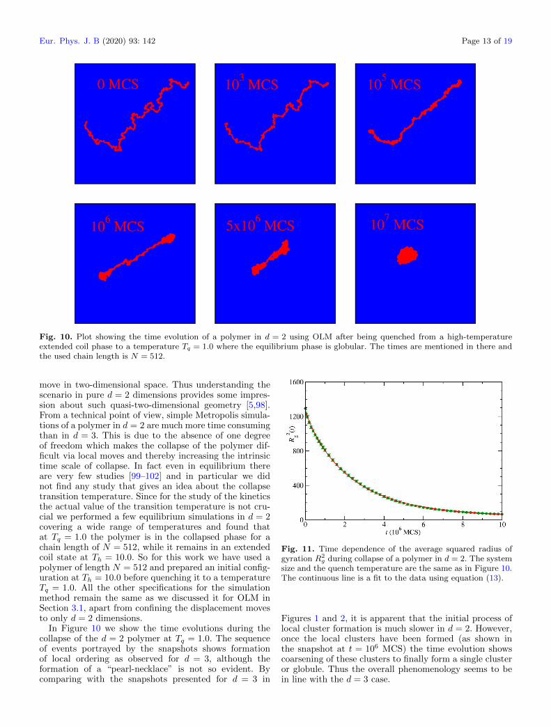
Fig. 10. Plot showing the time evolution of a polymer in d = 2 using OLM after being quenched from a high-temperatureextended coil phase to a temperature Tq = 1.0 where the equilibrium phase is globular. The times are mentioned in there andthe used chain length is N = 512.

move in two-dimensional space. Thus understanding thescenario in pure d = 2 dimensions provides some impres-sion about such quasi-two-dimensional geometry [5,98].From a technical point of view, simple Metropolis simula-tions of a polymer in d = 2 are much more time consumingthan in d = 3. This is due to the absence of one degreeof freedom which makes the collapse of the polymer dif-ficult via local moves and thereby increasing the intrinsictime scale of collapse. In fact even in equilibrium thereare very few studies [99–102] and in particular we didnot find any study that gives an idea about the collapsetransition temperature. Since for the study of the kineticsthe actual value of the transition temperature is not cru-cial we performed a few equilibrium simulations in d = 2covering a wide range of temperatures and found thatat Tq = 1.0 the polymer is in the collapsed phase for achain length of N = 512, while it remains in an extendedcoil state at Th = 10.0. So for this work we have used apolymer of length N = 512 and prepared an initial config-uration at Th = 10.0 before quenching it to a temperatureTq = 1.0. All the other specifications for the simulationmethod remain the same as we discussed it for OLM inSection 3.1, apart from confining the displacement movesto only d = 2 dimensions.

In Figure 10 we show the time evolutions during thecollapse of the d = 2 polymer at Tq = 1.0. The sequenceof events portrayed by the snapshots shows formationof local ordering as observed for d = 3, although theformation of a “pearl-necklace” is not so evident. Bycomparing with the snapshots presented for d = 3 in

Fig. 11. Time dependence of the average squared radius ofgyration R2

g during collapse of a polymer in d = 2. The systemsize and the quench temperature are the same as in Figure 10.The continuous line is a fit to the data using equation (13).

Figures 1 and 2, it is apparent that the initial process oflocal cluster formation is much slower in d = 2. However,once the local clusters have been formed (as shown inthe snapshot at t = 106 MCS) the time evolution showscoarsening of these clusters to finally form a single clusteror globule. Thus the overall phenomenology seems to bein line with the d = 3 case.



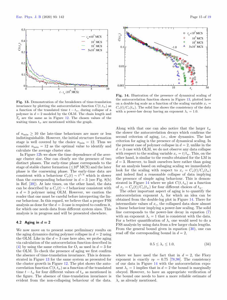
Following what has been done for the d = 3 case, atfirst we look at the time dependence of the overall size ofthe polymer by monitoring the squared radius of gyra-tion R2

g. In Figure 11 we show the corresponding plot

of R2g (calculated as an average over 300 different initial

realizations). Like in the d = 3 case, the decay of R2g can

be described quite well via the empirical relation men-tioned in equation (13). The best fit obtained is plottedas a continuous line in the plot. The obtained value of thenon-trivial parameter β in this fitting is ≈ 0.89, which iscompatible with the d = 3 case [39]. Still, the dependenceof β on the chain length N would be worth investigatingand will be presented elsewhere. Along the same line anunderstanding of the scaling of the collapse time with thechain length will be interesting to compare with the d = 3case. As this Colloquium is focused more on the clustercoarsening and aging during the collapse, here, we abstainourselves from presenting results concerning the scaling ofthe collapse time.

4.1 Cluster coarsening in d = 2

As can be seen from the snapshots in Figure 10, duringthe course of the collapse, like in d = 3, also for d = 2 onenotices formation of local clusters which via coalescencewith each other merge into bigger clusters and eventuallyform a single cluster or globule. We measure the averagecluster size in the following way. First we calculate thetotal numbers of monomers in the nearest vicinity of theith monomer as

ni =N∑j=1

Θ(rc − rij), (32)

where rc is the cutoff distance used in the nonbondedenergy (9) and Θ is the Heaviside step function. If ni ≥nmin, where nmin is a tunable lower cutoff, this is inter-preted as signal for a cluster around the ith monomerthat contains at least those ni closeby monomers. Notethat by construction we treat agglomerates of less thannmin monomers as random fluctuation or noise and do notclassify them as a cluster. By performing this constructionfor all N monomers, one obtains the number of monomersthat are inside a cluster. This number, however, wouldgreatly overestimate the total number of clusters sinceneighbouring monomers typically signal one and the samecluster. We remove this overcounting by considering theassociated Venn diagram, that is for each monomer withni ≥ nmin we associate a set Ai containing the ni neigh-bouring monomers satisfying the Θ-constraint in (32) andthen check the intersection of different sets Ai and Aj .If the intersection is the empty set, the clusters associ-ated with monomers i and j are different, otherwise theith and jth monomers belong to the same cluster formedby the union of Ai and Aj (and hence consisting of morethan max{ni, nj} monomers). The resulting set Ai ∪ Ajobtained this way could again be intersecting with anotherset which can be tackled in the same way. Thus we do thisexercise repeatedly until we get a number of discrete setsthat correspond to the discrete clusters.

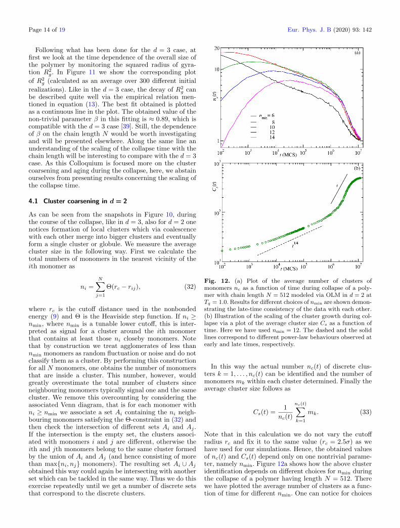
Fig. 12. (a) Plot of the average number of clusters ofmonomers nc as a function of time during collapse of a poly-mer with chain length N = 512 modeled via OLM in d = 2 atTq = 1.0. Results for different choices of nmin are shown demon-strating the late-time consistency of the data with each other.(b) Illustration of the scaling of the cluster growth during col-lapse via a plot of the average cluster size Cs as a function oftime. Here we have used nmin = 12. The dashed and the solidlines correspond to different power-law behaviours observed atearly and late times, respectively.

In this way the actual number nc(t) of discrete clus-ters k = 1, . . . , nc(t) can be identified and the number ofmonomers mk within each cluster determined. Finally theaverage cluster size follows as

Cs(t) =1

nc(t)

nc(t)∑k=1

mk. (33)

Note that in this calculation we do not vary the cutoffradius rc and fix it to the same value (rc = 2.5σ) as wehave used for our simulations. Hence, the obtained valuesof nc(t) and Cs(t) depend only on one nontrivial parame-ter, namely nmin. Figure 12a shows how the above clusteridentification depends on different choices for nmin duringthe collapse of a polymer having length N = 512. Therewe have plotted the average number of clusters as a func-tion of time for different nmin. One can notice for choices



Fig. 13. Demonstration of the breakdown of time-translationinvariance by plotting the autocorrelation function C(t, tw) asa function of the translated time t − tw, during collapse of apolymer in d = 2 modeled by the OLM. The chain length andTq are the same as in Figure 12. The chosen values of thewaiting times tw are mentioned within the graph.

of nmin ≥ 10 the late-time behaviours are more or lessindistinguishable. However, the initial structure formationstage is well covered by the choice nmin = 12. Thus weconsider nmin = 12 as the optimal value to identify andcalculate the average cluster size.

In Figure 12b we show the time dependence of the aver-age cluster size. One can clearly see the presence of twodistinct phases. The early-time phase corresponds to thestage of stable cluster formation (≤106 MCS) and the laterphase is the coarsening phase. The early-time data areconsistent with a behaviour Cs(t) ∼ t1/4 which is slowerthan the corresponding behaviour in d = 3 (see Fig. 8(b)in Ref. [39]). At late times, on the other hand, the datacan be described by a Cs(t) ∼ t behaviour consistent witha d = 3 polymer using OLM. However, we caution thereader that one must be careful before interpreting the lin-ear behaviour. In this regard, we believe that a proper FSSanalysis as done for the d = 3 case is required to confirm it,for which one needs data from different system sizes. Thisanalysis is in progress and will be presented elsewhere.

4.2 Aging in d = 2

We now move on to present some preliminary results onthe aging dynamics during polymer collapse in d = 2 usingthe OLM. Like in the d = 3 case here also, we probe agingvia calculation of the autocorrelation function described in(4) by using the same criterion for Oi as used in d = 3 forthe OLM. To check the presence of aging we first confirmthe absence of time-translation invariance. This is demon-strated in Figure 13 for the same system as presented forthe cluster growth in Figure 12. The plot shows the auto-correlation function C(t, tw) as a function of the translatedtime t− tw for four different values of tw as mentioned inthe figure. The absence of time-translation invariance isevident from the non-collapsing behaviour of the data.

Fig. 14. Illustration of the presence of dynamical scaling ofthe autocorrelation function shown in Figure 13, plotted hereon a double-log scale as a function of the scaling variable xc =Cs(t)/Cs(tw). The solid line shows the consistency of the datawith a power-law decay having an exponent λc = 1.0.

Along with that one can also notice that the larger twthe slower the autocorrelation decays which confirms thesecond criterion of aging, i.e., slow dynamics. The lastcriterion for aging is the presence of dynamical scaling. Inthe present case of polymer collapse in d = 2, unlike in thed = 3 case with OLM, we do not observe any data collapsewith respect to the scaling variable xc = t/tw. This, on theother hand, is similar to the results obtained for the LM ind = 3. However, to limit ourselves here rather than goingfor an analysis based on subaging scaling we immediatelylook for the scaling with respect to xc = Cs(t)/Cs(tw)and indeed find a reasonable collapse of data implyingthe presence of simple aging behaviour. This is demon-strated in Figure 14 where we plot C(t, tw) as a functionof xc = Cs(t)/Cs(tw) for four different choices of tw.

The other important aspect of aging is to quantify theautocorrelation exponent λc for which an idea can beobtained from the double-log plot in Figure 14. There forintermediate values of xc, the collapsed data show almosta linear behaviour implying a power-law scaling. The solidline corresponds to the power-law decay in equation (7)with an exponent λc = 1 that is consistent with the data.For a better quantification of λc one would need to do aFSS analysis by using data from a few larger chain lengths.From the general bound given in equation (30), one canread off the corresponding bound in d = 2,

0.5 ≤ λc ≤ 1.0, (34)

where we have used the fact that in d = 2, the Floryexponent is exactly νF = 0.75 [78,98]. The consistencyof our data in Figure 14 with the autocorrelation expo-nent λc = 1 implies that in d = 2 the bound is marginallyobeyed. However, to have an appropriate verification ofthe bound one needs to have a more reliable estimate ofλc as already mentioned.



5 Conclusion and outlook

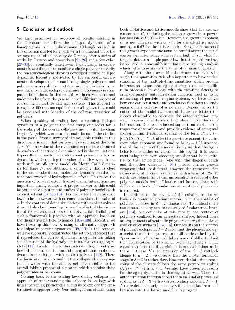
We have presented an overview of results existing inthe literature regarding the collapse dynamics of ahomopolymer in d = 3 dimensions. Although research inthis direction started long back with the proposition of thesausage model of collapse by de Gennes, after a series ofworks by Dawson and co-workers [21–26] and a few other[27–33], it eventually faded away. Particularly, in experi-ments it was difficult to monitor a single polymer to verifythe phenomenological theories developed around collapsedynamics. Recently, motivated by the successful experi-mental development for monitoring single polymers andpolymers in very dilute solutions, we have provided somenew insights in the collapse dynamics of polymers via com-puter simulations. In this regard, we borrowed tools andunderstanding from the general nonequilibrium process ofcoarsening in particle and spin systems. This allowed usto explore different nonequilibrium scaling laws that couldbe associated with kinetics of the collapse transition ofpolymers.

When speaking of scaling laws concerning collapsedynamics of a polymer the first thing one looks for isthe scaling of the overall collapse time τc with the chainlength N (which was also the main focus of the studiesin the past). From a survey of the available results in thisdirection it is clear that for power-law scaling of the formτc ∼ Nz, the value of the dynamical exponent z obtaineddepends on the intrinsic dynamics used in the simulations.Especially one has to be careful about presence of hydro-dynamics while quoting the value of z. However, in ourwork with an off-lattice model via Monte Carlo dynam-ics for large N , we obtained a value of z that is closeto the one obtained from molecular dynamics simulationswith preservation of hydrodynamic effects. This raises thequestion of to what extent hydrodynamic interactions areimportant during collapse. A proper answer to this couldbe obtained via systematic studies of polymer models withexplicit solvent [34,103,104]. For the latter there also existfew studies; however, with no consensus about the value ofz. In the context of doing simulations with explicit solventit would also be interesting to see the effect of the viscos-ity of the solvent particles on the dynamics. Building ofsuch a framework is possible with an approach based onthe dissipative particle dynamics [105–108]. Recently, wehave taken up this task by using an alternative approachto dissipative particle dynamics [109,110]. In this context,we have successfully constructed the set up and tested thatit reproduces the correct dynamics in equilibrium takingconsideration of the hydrodynamic interactions appropri-ately [111]. To add more to this understanding recently wehave also considered the task of doing all-atom moleculardynamics simulations with explicit solvent [112]. Therethe focus is on understanding the collapse of a polypep-tide in water with the aim to get new insights to theoverall folding process of a protein which contains thesepolypeptides as backbone.

Coming back to the scaling laws during collapse ourapproach of understanding the collapse in analogy withusual coarsening phenomena allows us to explore the clus-ter kinetics appropriately. Our findings from studies using

both off-lattice and lattice models show that the averagecluster size Cs(t) during the collapse grows in a power-law fashion as Cs(t) ∼ tαc . However, the growth exponentαc is not universal with αc ≈ 1 for the off-lattice modeland αc ≈ 0.62 for the lattice model. For quantification ofthis growth exponent one must be careful about the initialcluster formation stage which sets a high off-set while fit-ting the data to a simple power law. In this regard, we haveintroduced a nonequilibrium finite-size scaling analysiswhich helps to estimate the value of αc unambiguously.

Along with the growth kinetics where one deals withsingle-time quantities, it is also important to have under-standing of the multiple-time quantities which provideinformation about the aging during such nonequilib-rium processes. In analogy with the two-time density ororder-parameter autocorrelation function used in usualcoarsening of particle or spins systems, we have shownhow one can construct autocorrelation functions to studyaging during collapse of a polymer. Depending on thenature of the model (whether off-lattice or lattice) thechosen observable to calculate the autocorrelation mayvary; however, qualitatively they should give the sameinformation. Our results indeed support our choice of therespective observables and provide evidence of aging andcorresponding dynamical scaling of the form C(t, tw) ∼[Cs(t)/Cs(tw)]

−λc . Unlike the growth exponent, the auto-correlation exponent was found to be λc = 1.25 irrespec-tive of the nature of the model, implying that the agingbehaviour is rather universal. In this regard, it is worthmentioning that even choosing two different bond crite-ria for the lattice model (one with the diagonal bondsand the other without it [40]) yielded cluster growthexponents that are different, however, the autocorrelationexponent λc still remains universal with a value of 1.25. Tocheck the robustness of this universality, a study of otherpolymer models both off-lattice and lattice, along withdifferent methods of simulations as mentioned previouslyis required.

In addition to the review of the existing results wehave also presented preliminary results in the context ofpolymer collapse in d = 2 dimensions. To understand atwo-dimensional system is not only of fundamental inter-est [113], but could be of relevance in the context ofpolymers confined to an attractive surface. Indeed thereare experiments of synthetic polymers on two-dimensionalgold or silver surfaces [114,115]. Our results on the kineticsof polymer collapse in d = 2 show that the phenomenologyassociated with this process can still be described by the“pearl-necklace” picture of Halperin and Goldbart, albeitthe identification of the small pearl-like clusters whichcoarsen to form the final globule is not as distinct as inthe d = 3 case. Via an extension of the d = 3 method-ologies to d = 2 , we observe that the cluster formationstage in d = 2 is rather slow. However, the late-time coars-ening of the clusters follows the same power-law scalingCs(t) ∼ tαc with αc ≈ 1. We also have presented resultsfor the aging dynamics in this regard as well. There theautocorrelation function shows the same kind of power-lawscaling as in d = 3 with a corresponding exponent λc ≈ 1.A more detailed study not only with the off-lattice modelbut also with the lattice model is in progress.



Finally, we feel that this novel approach of under-standing the collapse dynamics of polymers from theperspective of usual coarsening studies of particle andspin systems shall serve as a general platform whichcould be used to analyze the nonequilibrium evolution ofmacromolecules in general across any conformational tran-sition. Of course, due to their distinct features, for eachclass of this transition the associated techniques shall bemodified accordingly. One has to choose the appropriateproperties of the system and find out the best quantitiesthat describe the corresponding transition appropriatelyin nonequilibrium. For example, one can look at the helix-coil transition of macromolecules as well [116,117]. Therecertainly the average cluster size would not work as a suit-able quantity to monitor the kinetics. Rather one maydefine some local helical order parameter and look at thecorresponding time dependence.

Open access funding provided by Projekt DEAL. This projectwas funded by the Deutsche Forschungsgemeinschaft (DFG,German Research Foundation) under project Nos. JA 483/33-1 and 189 853 844 – SFB/TRR 102 (project B04), and theDeutsch-Franzosische Hochschule (DFH-UFA) through theDoctoral College “L4” under Grant No. CDFA-02-07. We fur-ther acknowledge support by the Leipzig Graduate School ofNatural Sciences “BuildMoNa”.

Author contribution statement

S.M. planned the structure of the manuscript with inputsfrom the co-authors. All the authors contributed equallyin writing and developing the text.

Open Access This is an open access article distributedunder the terms of the Creative Commons AttributionLicense (http://creativecommons.org/licenses/by/4.0), whichpermits unrestricted use, distribution, and reproduction in anymedium, provided the original work is properly cited.

Publisher’s Note The EPJ Publishers remain neutral withregard to jurisdictional claims in published maps and institu-tional affiliations.

References

1. L.D. Landau, E.M. Lifshitz, Statistical Physics(Pergamon Press, London, 1958)

2. H.E. Stanley, Introduction to Phase Transitions andCritical Phenomena (Clarendon Press, Oxford, 1971)

3. A. Onuki, Phase Transition Dynamics (CambridgeUniversity Press, Cambridge, 2002)

4. S. Puri, V. Wadhawan, eds., Kinetics of PhaseTransitions (CRC Press, Boca Raton, 2009)

5. P.-G. de Gennes, Scaling Concepts in Polymer Physics(AIP, Melville, New York, 1980)

6. M. Doi, S.F. Edwards, The Theory of Polymer Dynamics(Clarendon Press, Oxford, 1986)

7. J. des Cloizeaux, G. Jannink, Polymers in Solution(Clarendon Press, Oxford, 1990)

8. M. Rubinstein, R.H. Colby, Polymer Physics (OxfordUniversity Press, New York, 2003)

9. W.H. Stockmayer, Macromol. Chem. Phys. 35, 54 (1960)10. I. Nishio, S.-T. Sun, G. Swislow, T. Tanaka, Nature 281,

208 (1979)11. C.J. Camacho, D. Thirumalai, Proc. Natl. Acad. Sci.

USA 90, 6369 (1993)12. L. Pollack, M.W. Tate, A.C. Finnefrock, C. Kalidas,

S. Trotter, N.C. Darnton, L. Lurio, R.H. Austin, C.A.Batt, S.M. Gruner et al., Phys. Rev. Lett. 86, 4962 (2001)

13. M. Sadqi, L.J. Lapidus, V. Munoz, Proc. Natl. Acad. Sci.USA 100, 12117 (2003)

14. G. Haran, Curr. Opin. Struct. Biol. 22, 14 (2012)15. G. Reddy, D. Thirumalai, J. Phys. Chem. B 121, 995

(2017)16. B. Chu, Q. Ying, A.Y. Grosberg, Macromolecules 28, 180

(1995)17. B. Schuler, E.A. Lipman, W.A. Eaton, Nature 419, 743

(2002)18. J. Xu, Z. Zhu, S. Luo, C. Wu, S. Liu, Phys. Rev. Lett.

96, 027802 (2006)19. M. Tress, E.U. Mapesa, W. Kossack, W.K. Kipnusu,

M. Reiche, F. Kremer, Science 341, 1371 (2013)20. P.-G. de Gennes, J. Phys. Lett. 46, 639 (1985)21. A. Byrne, P. Kiernan, D. Green, K.A. Dawson, J. Chem.

Phys. 102, 573 (1995)22. E.G. Timoshenko, Yu.A. Kuznetsov, K.A. Dawson, J.

Chem. Phys. 102, 1816 (1995)23. Yu.A. Kuznetsov, E.G. Timoshenko, K.A. Dawson, J.



Chem. Phys. 105, 7116 (1996)26. K.A. Dawson, E.G. Timoshenko, Yu.A. Kuznetsov,

Physica A 236, 58 (1997)27. E. Pitard, H. Orland, Europhys. Lett. 41, 467 (1998)28. L.I. Klushin, J. Chem. Phys. 108, 7917 (1998)29. A. Halperin, P.M. Goldbart, Phys. Rev. E 61, 565

(2000)30. N. Kikuchi, A. Gent, J.M. Yeomans, Eur. Phys. J. E 9,

63 (2002)31. C.F. Abrams, N.K. Lee, S.P. Obukhov, Europhys. Lett.

59, 391 (2002)32. A. Montesi, M. Pasquali, F.C. MacKintosh, Phys. Rev. E

69, 021916 (2004)33. N. Kikuchi, J.F. Ryder, C.M. Pooley, J.M. Yeomans,

Phys. Rev. E 71, 061804 (2005)34. T.T. Pham, M. Bajaj, J.R. Prakash, Soft Matter 4, 1196

(2008)35. J. Guo, H. Liang, Z.G. Wang, J. Chem. Phys. 134, 244904

(2011)36. S. Majumder, W. Janke, Europhys. Lett. 110, 58001

(2015)37. S. Majumder, W. Janke, Phys. Rev. E 93, 032506

(2016)38. S. Majumder, W. Janke, J. Phys.: Conf. Ser. 750, 012020

(2016)39. S. Majumder, J. Zierenberg, W. Janke, Soft Matter 13,

1276 (2017)40. H. Christiansen, S. Majumder, W. Janke, J. Chem. Phys.

147, 094902 (2017)41. S. Majumder, H. Christiansen, W. Janke, J. Phys.: Conf.

Ser. 955, 012008 (2018)42. P.C. Hohenberg, B.I. Halperin, Rev. Mod. Phys. 49, 435

(1977)


http://creativecommons.org/licenses/by/4.0


43. D. Frenkel, B. Smit, Understanding MolecularSimulation: From Algorithms to Applications (AcademicPress, San Diego, 2001)

44. P.E. Rouse, J. Chem. Phys. 21, 1272 (1953)45. B.H. Zimm, J. Chem. Phys. 24, 269 (1956)46. W. Janke, in Order, Disorder and Criticality: Advanced

Problems of Phase Transition Theory, edited by Y.Holovatch (World Scientific, Singapore, 2012), Vol. 3,p. 93

47. W. Janke, in Order, Disorder and Criticality: AdvancedProblems of Phase Transition Theory, edited by Y.Holovatch (World Scientific, Singapore, 2018), Vol. 5,p. 173

48. A.J. Bray, Adv. Phys. 51, 481 (2002)49. R. Shimizu, H. Tanaka, Nat. Commun. 6, 7407 (2015)50. S. Basu, S. Majumder, S. Sutradhar, S.K. Das, R. Paul,

Europhys. Lett. 116, 56003 (2017)51. H. Christiansen, S. Majumder, W. Janke, Phys. Rev. E

99, 011301(R) (2019)52. W. Janke, H. Christiansen, S. Majumder, J. Phys.: Conf.

Ser. 1163, 012002 (2019)53. F. Corberi, E. Lippiello, P. Politi, J. Stat. Phys. 176, 510

(2019)54. I.M. Lifshitz, V.V. Slyozov, J. Phys. Chem. Solids 19, 35

(1961)55. S.M. Allen, J.W. Cahn, Acta Metall. 27, 1085 (1979)56. E.D. Siggia, Phys. Rev. A 20, 595 (1979)57. H. Furukawa, Phys. Rev. A 31, 1103 (1985)58. M. Henkel, M. Pleimling, in Non-Equilibrium Phase

Transitions, Ageing and Dynamical Scaling far fromEquilibrium (Springer, Heidelberg, 2010), Vol. 2

59. M. Zannetti, in Kinetics of Phase Transitions, edited byS. Puri, V. Wadhawan (CRC Press, Boca Raton, 2009),p. 153

60. J.-P. Bouchaud, in Soft and Fragile Matter:Nonequilibrium Dynamics, Metastability and Flow,edited by M. Cates, M.R. Evans (IOP, Bristol, 2000),p. 285

61. H.E. Castillo, C. Chamon, L.F. Cugliandolo, M.P.Kennett, Phys. Rev. Lett. 88, 237201 (2002)

62. D.S. Fisher, D.A. Huse, Phys. Rev. B 38, 373 (1988)63. F. Liu, G.F. Mazenko, Phys. Rev. B 44, 9185 (1991)64. E. Lorenz, W. Janke, Europhys. Lett. 77, 10003 (2007)65. J. Midya, S. Majumder, S.K. Das, J. Phys.: Condens.

Matter 26, 452202 (2014)66. C. Yeung, M. Rao, R.C. Desai, Phys. Rev. E 53, 3073

(1996)67. E. Pitard, J.-P. Bouchaud, Eur. Phys. J. E 5, 133 (2001)68. N.V. Dokholyan, E. Pitard, S.V. Buldyrev, H.E. Stanley,

Phys. Rev. E 65, 030801(R) (2002)69. M. Cloitre, R. Borrega, L. Leibler, Phys. Rev. Lett. 85,

4819 (2000)70. P. Bursac, G. Lenormand, B. Fabry, M. Oliver, D.A.

Weitz, V. Viasnoff, J.P. Butler, J.J. Fredberg, Nat. Mater.4, 557 (2005)

71. P. Wang, C. Song, H.A. Makse, Nat. Phys. 2, 526 (2006)72. A. Milchev, A. Bhattacharya, K. Binder, Macromolecules

34, 1881 (2001)73. J.S. Shaffer, J. Chem. Phys. 101, 4205 (1994)74. T. Dotera, A. Hatano, J. Chem. Phys. 105, 8413 (1996)75. I. Carmesin, K. Kremer, Macromolecules 21, 2819

(1988)76. G. Subramanian, S. Shanbhag, J. Chem. Phys. 129,

144904 (2008)

77. D.P. Landau, K. Binder, A Guide to Monte CarloSimulations in Statistical Physics (Cambridge UniversityPress, Cambridge, 2009)

78. P.J. Flory, Principles of Polymer Chemistry (CornellUniversity Press, Ithaca, NY, 1953)

79. S. Majumder, S.K. Das, Europhys. Lett. 95, 46002 (2011)80. S. Majumder, S.K. Das, Phys. Rev. E 84, 021110 (2011)81. S. Majumder, S.K. Das, W. Janke, Phys. Rev. E 98,

042142 (2018)82. S. Majumder, S.K. Das, Phys. Rev. E 81, 050102(R)

(2010)83. S.K. Das, S. Roy, S. Majumder, S. Ahmad, Europhys.

Lett. 97, 66006 (2012)84. S. Majumder, S.K. Das, Phys. Chem. Chem. Phys. 15,

13209 (2013)85. M.E. Fisher, in Critical Phenomena, edited by M.S.

Green (Academic Press, London, 1971), p. 186. V. Privman, Finite Size Scaling and the Numerical

Simulations of Statistical Systems (World Scientific,Singapore, 1990)

87. V. Privman, M.E. Fisher, Phys. Rev. B 30, 322 (1984)88. C.K. Hu, C.-Y Lin, J.-A. Chen, Phys. Rev. Lett. 75, 193

(1995)89. H.J. Hilhorst, J.M.J. van Leeuwen, Phys. Rev. Lett. 47,

1188 (1981)90. D. Herisson, M. Ocio, Eur. Phys. J. B 40, 283 (2004)91. D. Parker, F. Ladieu, J. Hammann, E. Vincent, Phys.

Rev. B 74, 184432 (2006)92. H. Christiansen, S. Majumder, M. Henkel, W. Janke,

arXiv:1906.11815 (2019)93. J. Kurchan, Phys. Rev. E 66, 017101 (2002)94. R. Paul, G. Schehr, H. Rieger, Phys. Rev. E 75,

030104(R) (2007)95. H. Park, M. Pleimling, Phys. Rev. B 82, 144406 (2010)96. N. Clisby, Phys. Rev. Lett. 104, 055702 (2010)97. N. Clisby, B. Dunweg, Phys. Rev. E 94, 052102 (2016)98. C. Vanderzande, Lattice Models of Polymers (Cambridge

University Press, Cambridge, 1998)99. M. Wittkop, S. Kreitmeier, D. Goritz, J. Chem. Phys.

104, 3373 (1996)100. J.M. Polson, M.J. Zuckermann, J. Chem. Phys. 113, 1283

(2000)101. P. Grassberger, H.-P. Hsu, Phys. Rev. E 65, 031807

(2002)102. H. Zhou, J. Zhou, Z.C. Ou-Yang, S. Kumar, Phys. Rev.

Lett. 97, 158302 (2006)103. R. Chang, A. Yethiraj, J. Chem. Phys. 114, 7688 (2001)104. J.M. Polson, M.J. Zuckermann, J. Chem. Phys. 116, 7244

(2002)105. P.J. Hoogerbrugge, J.M.V.A. Koelman, Europhys. Lett.

19, 155 (1992)106. P. Espanol, P. Warren, Europhys. Lett. 30, 191 (1995)107. R.D. Groot, P.B. Warren, J. Chem. Phys. 107, 4423

(1997)108. P. Espanol, P.B. Warren, J. Chem. Phys. 146, 150901

(2017)109. C.P. Lowe, Europhys. Lett. 47, (1999) 145110. E.A. Koopman, C.P. Lowe, J. Chem. Phys. 124, 204103

(2006)111. S. Majumder, H. Christiansen, W. Janke, J. Phys.: Conf.

Ser. 1163, 012072 (2019)112. S. Majumder, U.H.E. Hansmann, W. Janke,

Macromolecules 52, 5491 (2019)113. J. Midya, S.K. Das, Phys. Rev. Lett. 118, 165701 (2017)


https://arxiv.org/abs/1906.11815


114. S. Forster, W. Widdra, J. Chem. Phys. 141, 054713(2014)

115. S. Forster, E. Kohl, M. Ivanov, J. Gross, W. Widdra,W. Janke, J. Chem. Phys. 141, 164701 (2014)

116. E. Arashiro, J.R. Drugowich de Felıcio, U.H.E.Hansmann, Phys. Rev. E 73, 040902(R) (2006)

117. E. Arashiro, J.R. Drugowich de Felıcio, U.H.E.Hansmann, J. Chem. Phys. 126, 045107 (2007)


Understanding nonequilibrium scaling laws governing ...

Documents