Fourier Analysis and Symmetry Fourier Analysis and Symmetry Quantum Theory for the Computer Age Unit 3 Quantum Theory for the Computer Age Unit 3 HarterSoft –LearnIt Unit 3 Fourier Analysis and Symmetry ----1

Welcome message from author
This document is posted to help you gain knowledge. Please leave a comment to let me know what you think about it! Share it to your friends and learn new things together.
Transcript
Fourier Analysisand
Symmetry
Fourier Analysisand
Symmetry
Quantum Theory for theComputer Age
Unit 3
Quantum Theory for theComputer Age
Unit 3
HarterSoft –LearnIt Unit 3 Fourier Analysis and Symmetry ----1
2
Unit 3 Fourier Analysis and SymmetryUnit 2 discussed quantum ei(k•r-ω t)-wave propagation in space and time and introduced
wavevector and frequency (ck,ω)-space while deriving the basic Einstein relativistic transformations and Planck-deBroglie quantum relations. But, what are ei(k•r-ω t)-waves? One
answer comes from understanding relations between space-time (x,ct) and (ck,ω)-space known as Fourier transformations. Unit 3 begins with discussions of Fourier <!|!> transformation matrices and shows their connection to translational symmetry. This with Planckʼs axiom gives the quantum equation of motion known as Schodingerʼs time equation, the evolution operator, and its generator, the quantum Hamiltonain operator, the sine qua non of Schrodinger theory. Unit 3 continues with a detailed description of quantum beats and revivals using symmetry analysis. The final chapter describes 2-state and spin-1/2 systems while introducing U(2) symmetry analysis.
W. G. Harter
Department of Physics
University of Arkansas
Fayetteville
Hardware and Software by
HARTER-SoftElegant Educational Tools Since 2001
©2013 W. G. Harter Chapter 7 Fourier transformation matrices ! 7--
Unit 3 Fourier Analysis and Symmetry
QMfor
AMOPΨ
Chapter 7Fourier Transformation Matrices
W. G. Harter
HarterSoft –LearnIt Unit 3 Fourier Analysis and Symmetry ----3
4
.........................................................CHAPTER 7. FOURIER TRANSFORMATION MATRICES! 1
........................................................................................................7.1 Continuous but bounded x. Discrete but unbounded k! 1........................................................................................................................................................(a) Orthonormality axiom-3! 2
...........................................................................................................................................................(b) Completeness axiom-4! 3...................................................................................................................................(c) Fourier series representation of a state! 3....................................................................................................................................(d) Bohr dispersion relation and energies! 3
...............................................................................................................(e) Sine and cosine Fourier series worth remembering! 4
............................................................................................7.2 Continuous and unbounded x. Continuous and unbounded k! 7.....................................................................................................................................................(a) Fourier integral transforms! 7
................................................................................................................................(b) Fourier coefficients: Their many names! 8.......................................................................................................................(c) Time: Fourier transforms worth remembering! 9
...............................................................................................................7.3 Discrete and bounded x. Discrete and bounded k! 13....................................................................................................................................(a) N-nary counting for N-state systems! 15
..........................................................................................................................(b) Discrete orthonormality and completeness! 15............................................................................................................................(c) Discrete Fourier transformation matrices! 16
................................................................................................................................(d) Intoducing aliases and Brillouin zones! 17
................................................................................................................................................................Problems for Chapter 7! 20
.......................................................................CHAPTER 8. FOURIER SYMMETRY ANALYSIS ! 3
......................................................................................................................8.1. Introducing Cyclic Symmetry: A C6 example! 3..................................................................................................................(a) Cyclic symmetry CN: A 6-quantum-dot analyzer! 3
............................................................................................................................(b) CN Symmetry groups and representations! 5..........................................................................................................................................(c) So what’s a group representation?! 6
..................................................................................................8.2 CN Spectral Decomposition: Solving a C6 transfer matrix! 7................................................................................................................(a) Spectral decomposition of symmetry operators rp! 7
.............................................................................................(b) Writing transfer operator T in terms of symmetry operators rp! 9.....................................................................................................................(c) Spectral decomposition of transfer operator T! 10
................................................................................................................................What do the km- eigensolutions mean?! 11........................................................................................................(d) OK, where did those eikx wavefunctions come from?! 12
.................................................................................................................................8.3 Related Symmetry Analysis Examples! 13.........................................................................................................................................................(a) Dihedral symmetry D2! 14
................................................................................................................................................................D2 group structure! 14.....................................................................................................D2 spectral decomposition: The old “1=1•1 trick” again! 15
...................................................................................................................Spectral decomposition of D2 transfer matrices! 15..................................................................................................................(b) Outer product structure: Double qubit registers! 16
............................................................................................................................................Big-endian versus Little-endian! 16..................................................................................................................C6 is product C3× C2 (but C4 is NOT C2× C2) ! 17
................................................................................................................................................................Symmetry Catalog! 17
...............................................................................................................................................................Problems for Chapter 8.! 18
...................................................CHAPTER 9. TIME EVOLUTION AND FOURIER DYNAMICS! 1
©2013 W. G. Harter Chapter 7 Fourier transformation matrices ! 7--
.........................................................................................................................................................9.1 Time Evolution Operator! 1...............................................................................................................................................(a) Planck's oscillation hypothesis! 1
...................................................................................................................................................9.2 Schrodinger Time Equations! 3..................................................................................................(a) Schrodinger's time equations. Hamiltonian time generators! 3
..............................................................................................................................................(b) Schrodinger's matrix equations! 4...................................................................................................(c) Writing Hamiltonian H in terms of symmetry operators rp! 5
..................................................................................................................................................9.3 Schrodinger Eigen-Equations! 6...........................................................................................................(a) Solving Schrodinger's eigen-equations for C6 system! 8
.....................................................................................................................................(b) Energy spectrum and tunneling rates! 8.............................................................................................................................................................(c) Brillouin's boundary! 10
.................................................................................................................Effective mass: Another quantum view of inertia! 12.........................................................................................................(d) Bohr wavepacket dynamics: Uncertainty and revival! 16
.........................................................................................Semi-classical Theory: Farey Sums and Quantum Speed Limits! 16
......................................................................................................................................................9.4 Homo-cyclic Cn Revivals! 20...............................................................................................................................................(a) Two–state C2 systems: Beats! 20
..........................................................................................................................(b) Cn group structure: n=3, 4,...6 Eigenstates! 22......................................................................................................................(c) Cn dynamics: n=3, 4,...6 Fractional Revivals! 24
.....................................................................................................................................................Bohr vs. Bloch dispersion! 29
...............................................................................................................................................................Problems for Chapter 9.! 31
..........................................................................REVIEW TOPICS & FORMULAS FOR UNIT 3! 34
Expressing arbitrary wavefunctions or states in terms of spectral components or plane waves is known as Fourier analysis. Fourier transformation matrices relate space and time (coordinate) bases to wavevector and frequency (Energy-momentum) bases of plane waves. Fourier analysis comes in different flavors depending on whether various bases are discretely numbered or continuous. Chapter 7 compares the continuous coordinate bases of Bohr rotor states to the fully continuous plane wave states of an unbounded continuum. Then a discrete “quantum-dot” sytsem is introduced in which both coordinates and wavevectors are discrete. The later is the basis for the introduction of Fourier symmetry analysis in the following Chapter 8 and time evolution in Chapter 9. Discrete symmetry in space and time helps to clarify quantum beats and “revivals” which all quantum systems will exhibit to some degree.
HarterSoft –LearnIt Unit 3 Fourier Analysis and Symmetry ----5
2
....................................................CHAPTER 10. TWO-STATE EVOLUTION AND ANALOGIES! 4
................................................................................................................10.1 Mechanical Analogies to Schrodinger Dynamics 4.....................................................................................................................................(a). ABCD Symmetry operator analysis 6
.........................................................................................................................................10.2 The ABCD’s of 2-State Dynamics 8..............................................................................................................................(a) Asymmetric-Diagonal or C2A symmetry 8
..................................................................................................................................................(b) Bilateral or C2B symmetry 10...................................................................................................................C2B projectors and eigenstates: Normal modes 11
............................................................................................................Understanding C2B eigenstates: Tunneling splitting 12...........................................................................................Understanding C2B dynamics: Beats and transition frequency 13
...................................................................................................................................................(c) Circular or C2C symmetry 17............................................................................................................................R(2)=C∞ projectors and C2C eigenstates 18
...................................................Understanding C2C eigenstates: Zeeman-like splitting and coriolis or cyclotron motion 19..................................................................................................................Understanding C2C dynamics: Faraday rotation 22
....................................................................................................................................................10.3 Mixed A and B Symmetry 25................................................................................................(a) Asymmetric bilateral C2AB symmetry: Stark-like-splitting 25
....................................................................................................High field splitting: Strong C2A or weak C2B symmetry 26..............................................................Low field splitting: Strong C2B or weak C2A symmetry and A→B basis change 29
........................................................................................................................................................(b) Ammonia (NH3) maser 29.....................................................................................................................................C2AB Symmetry : Weyl reflections 31
..........................................................................................................................Unitary U(2) versus Special Unitary SU(2) 33................................................................................................................................Complete sets of commuting operators 33
..............................................................................................................10.4 Mixed ABCD Symmetry: U(2) quantum systems 34........................................................................................(a) ABC Symmetry catalog: Standing, moving, or galloping waves 35
....................................................................................A, B, and AB-Archetypes are standing waves (Linear polarization) 35.....................................................................................................C-Archetypes are moving waves (Circular polarization) 35
..................................................................................................….All others are galloping waves (Elliptical polarization) 35..............................................................................................................................................(b) General HABCD eigenvalues 36
....................................................................................................10.5 Spin-Vector Pictures for Two-State Quantum Systems 38..............................................................................................................................(a) Density operators and Pauli σ-operators 40
............................................................................................(b) Hamiltonian operators and Pauli-Jordan spin operators (J=S) 43....................................................................................................................................(c) Bloch equations and spin precession 44
.............................................................................................................................Magnetic spin precession (ESR, NMR,..) 45..................................................................................................................(d) Visualizing quantum dynamics as S-precession 46
Crank Ω polar angles (ϕ,ϑ ...............................................................................................) versus Spin S polar angles (α,β) 49........................................................................Hamilton’s generalization of exp(-iω t)=cosω t-isinω t : exp(-i σ t)=What? 51
.........................................................................................................................................................................Why the 1/2? 52
............................................................................................................................................................Problems for Chapter 10. 53
..........................................................................REVIEW TOPICS & FORMULAS FOR UNIT 3! 57......................................................................................................................U(2)-R(3) Two-State and Spin-Vector Summary 60
........................................................................................................Appendix 10.A. U(2) Angles and Spin Rotation Operators 2..............................................................................................................................(a) Equivalence transformations of rotations 5
....................................................................................................................(b) Euler equivalence transformations of 3-vectors 5...................................................................................................................(c) Euler angle goniometer: Double valued position 6
......................................................................................................................(d) Axis angle rotation: Double valued operation 11.....................................................................................................................(1) Combining rotations: U(2) group products 13
..........................................................................................................................(2) Mirror reflections and Hamilton's turns 13..............................................................................................................(3) Similarity transformation and Hamilton's turns 15
.................................................................................................................................(e) Quaternion and spinor algebra (again) 16.........................................................................................................................................Why rotations are such a big deal 17
©2013 W. G. Harter Chapter10 Two-State Time Evolution 10-

.............................................................................................................................Appendix 10.B Spin control and ellipsometry 1.........................................................................................................................(a). Polarization ellipsometry coordinate angles 6
.....................................................................................................................................(1) Type-A ellipsometry Euler angles 7
.....................................................................................................................................(2) Type-C ellipsometry Euler angles 9............................................................................................................................................(b) Beam evolution of polarization 13
............................................................................................................................................Problems for Appendix 10.A and B 14
HarterSoft –LearnIt Unit 3 Fourier Analysis and Symmetry 10-3
1
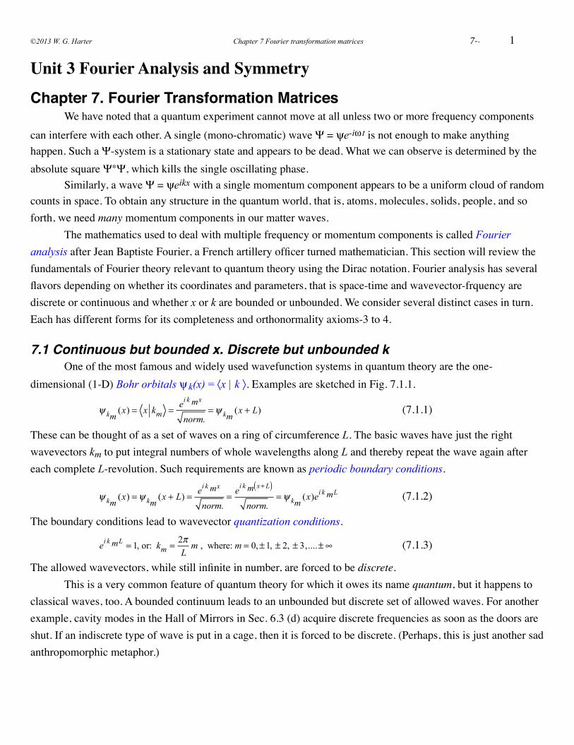
Unit 3 Fourier Analysis and SymmetryChapter 7. Fourier Transformation Matrices! We have noted that a quantum experiment cannot move at all unless two or more frequency components can interfere with each other. A single (mono-chromatic) wave Ψ = ψe-iω t is not enough to make anything happen. Such a Ψ-system is a stationary state and appears to be dead. What we can observe is determined by the absolute square Ψ∗Ψ, which kills the single oscillating phase.! Similarly, a wave Ψ = ψeikx with a single momentum component appears to be a uniform cloud of random counts in space. To obtain any structure in the quantum world, that is, atoms, molecules, solids, people, and so forth, we need many momentum components in our matter waves.! The mathematics used to deal with multiple frequency or momentum components is called Fourier analysis after Jean Baptiste Fourier, a French artillery officer turned mathematician. This section will review the fundamentals of Fourier theory relevant to quantum theory using the Dirac notation. Fourier analysis has several flavors depending on whether its coordinates and parameters, that is space-time and wavevector-frquency are discrete or continuous and whether x or k are bounded or unbounded. We consider several distinct cases in turn. Each has different forms for its completeness and orthonormality axioms-3 to 4.
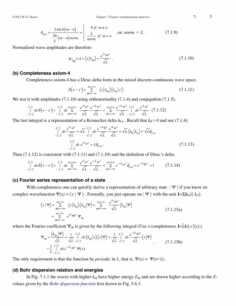
7.1 Continuous but bounded x. Discrete but unbounded k! One of the most famous and widely used wavefunction systems in quantum theory are the one-dimensional (1-D) Bohr orbitals ψ k(x) = 〈x | k 〉. Examples are sketched in Fig. 7.1.1.
! ! ψ km
(x) = x km = ei k mx
norm.=ψ km
(x + L) ! ! ! ! ! (7.1.1)
These can be thought of as a set of waves on a ring of circumference L. The basic waves have just the right wavevectors km to put integral numbers of whole wavelengths along L and thereby repeat the wave again after each complete L-revolution. Such requirements are known as periodic boundary conditions.
! ! ψ km
(x) =ψ km(x + L) = ei k mx
norm.= ei k m x+ L( )
norm.=ψ km
(x)ei k mL ! ! (7.1.2)
The boundary conditions lead to wavevector quantization conditions.
! ! ei k mL = 1, or: km = 2π
Lm , where: m = 0,±1, ± 2, ± 3,....± ∞ ! ! (7.1.3)
The allowed wavevectors, while still infinite in number, are forced to be discrete.! This is a very common feature of quantum theory for which it owes its name quantum, but it happens to classical waves, too. A bounded continuum leads to an unbounded but discrete set of allowed waves. For another example, cavity modes in the Hall of Mirrors in Sec. 6.3 (d) acquire discrete frequencies as soon as the doors are shut. If an indiscrete type of wave is put in a cage, then it is forced to be discrete. (Perhaps, this is just another sad anthropomorphic metaphor.)
©2013 W. G. Harter Chapter 7 Fourier transformation matrices ! 7--
! m or km
E
m=1m= -1m=0
m=2m= -2
m=3m= -3
m=4m= -4
m=5m= -5
m=6m= -6
L
m=0
L= 40
m= ±1m= ±2
m= ±3
m= ±4
m= ±5
m= ±6
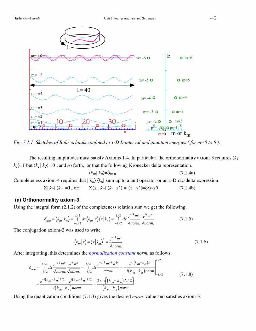
Fig. 7.1.1 Sketches of Bohr orbitals confined to 1-D L-interval and quantum energies ( for m=0 to 6 ).
! The resulting amplitudes must satisfy Axioms 1-4. In particular, the orthonormality axiom-3 requires 〈k1| k1〉=1 but 〈k1| k2〉 =0 , and so forth, or that the following Kronecker delta representation.! ! ! ! ! 〈km| kn〉=δm n ! ! ! ! ! (7.1.4a)Completeness axiom-4 requires that | kn〉 〈kn| sum up to a unit operator or an x-Dirac-delta expression.! ! Σ| kn〉 〈kn| =1,! or:! Σ 〈x | kn〉 〈kn| x' 〉 = 〈x | x' 〉=δ(x-x').! ! (7.1.4b)
(a) Orthonormality axiom-3Using the integral form (2.1.2) of the completeness relation sum we get the following.
! ! δm n = km kn = dx
−L / 2
L / 2∫ km x x kn = dx
−L / 2
L / 2∫
e−i k mx
norm.ei k nx
norm.! ! (7.1.5)
The conjugation axiom-2 was used to write
! ! ! !
km x = x km*= e−i k mx
norm.! ! ! ! ! (7.1.6)
After integrating, this determines the normalization constant norm. as follows.
!
δm n = dx−L / 2
L / 2∫
e−i k mx
norm.ei k nx
norm.= dx
−L / 2
L / 2∫
e−i k m−k n( )xnorm.
= e−i k m−k n( )x−i k m− k n( )norm.
−L / 2
L / 2
= e−i k m−k n( )L / 2 − ei k m−k n( )L / 2
−i k m− k n( )norm.=
2sin k m− k n( ) L / 2⎡⎣ ⎤⎦k m− k n( )norm.
! (7.1.8)
Using the quantization conditions (7.1.3) gives the desired norm. value and satisfies axiom-3.
HarterSoft –LearnIt Unit 3 Fourier Analysis and Symmetry ----2
3
! !
δm n =2sinπ m − n( )
2πL
m − n( )norm.=
0 if : m ≠ nL
norm. if : m = n
⎧
⎨⎪
⎩⎪
, or: norm. = L.! ! (7.1.9)
Normalized wave amplitudes are therefore
! ! ! ! ψ km
(x) = x km = ei k mx
L.! ! ! ! ! (7.1.10)
(b) Completeness axiom-4! Completeness axiom-4 has a Dirac-delta form in the mixed discrete-continuous wave space.
! ! ! ! δ x − x '( ) =
m=−∞
m=+∞∑ x km km x ' ! ! ! ! (7.1.11)
We test it with amplitudes (7.1.10) using orthonormality (7.1.4) and conjugation (7.1.5).
!
dx−L / 2
L / 2∫ δ x − x '( ) = dx
−L / 2
L / 2∫
n=−∞
n=+∞∑
ei k nx
L
e−i k nx '
L= e−i k nx '
Ln=−∞
n=+∞∑ dx
−L / 2
L / 2∫
ei k nx
L!(7.1.12)
The last integral is a representation of a Kronecker delta δ0,n . Recall that k0 =0 and use (7.1.4).
! ! !
dx−L / 2
L / 2∫
ei k nx
L= L dx
−L / 2
L / 2∫
e−i k 0x
L
ei k nx
L= L k0 kn = Lδ0 n
! ! ! !
dx−L / 2
L / 2∫ ei k nx = Lδ0 n .! ! ! ! ! ! (7.1.13)
Then (7.1.12) is consistent with (7.1.11) and (7.1.10) and the definition of Dirac’s delta.
!
dx−L / 2
L / 2∫ δ x − x '( ) = dx
−L / 2
L / 2∫
n=−∞
n=+∞∑
ei k nx
L
e−i k nx '
L= e−i k nx '
n=−∞
n=+∞∑ δ0 n = e−i k 0x ' = 1 ! (7.1.14)
(c) Fourier series representation of a state! With completeness one can quickly derive a representation of arbitrary state | Ψ 〉 if you know its complex wavefunction Ψ(x) = 〈 x | Ψ 〉 . Formally, you just operate on | Ψ 〉 with the unit 1=Σ|km〉〈 km |.
! !
x |Ψ =m=−∞
m=+∞∑ x km km Ψ =
m=−∞
m=+∞∑
ei k mx
Lkm Ψ
=m=−∞
m=+∞∑ ei k mx Ψm
! ! ! (7.1.15a)
where the Fourier coefficient Ψm is given by the following integral (Use x-completeness 1=∫dx| x 〉〈x |.)
! !
Ψm =km Ψ
L= 1
Ldx
−L / 2
L / 2∫ km x x Ψ = 1
Ldx
−L / 2
L / 2∫
e−i k mx
Lx Ψ
= 1L
dx−L / 2
L / 2∫ e−i k mx Ψ(x)
.! (7.1.15b)
The only requirement is that the function be periodic in L, that is, Ψ(x) = Ψ(x+L).
(d) Bohr dispersion relation and energies! In Fig. 7.1.1 the waves with higher km have higher energy Em and are drawn higher according to the E-values given by the Bohr dispersion function first drawn in Fig. 5.6.3.
©2013 W. G. Harter Chapter 7 Fourier transformation matrices ! 7--
! ! ! Em = ωm =
km( )22M
, where: pm = km = 2πL
m .! ! (7.1.16)
This is just a non-relativistic approximation for energy that neglects the rest energy Mc2 and higher order terms in (5.2.5b). It is kinetic energy only, that is KE = 1/2Mu2 = p2/2M with the momentum p=pm and wavevector k=km quantized by conditions (7.1.3). The dispersion function is then a simple parabola of discrete values as shown on the right hand side of Fig. 7.1.1. Note that each energy value Em , except E0, has two orthogonal wavefunctions ψ±km or states |±km〉 corresponding to pairs of oppositely moving wavevectors ±km on either side of the dispersion parabola. The |±km〉 are called degenerate states because they share a single energy Em. Such degenerate pairs are each an example of a U(2) two-state system. As long as the degeneracy remains, any unitary linear combination of the two states is also an eigenstate with the same frequency and energy E=hν.
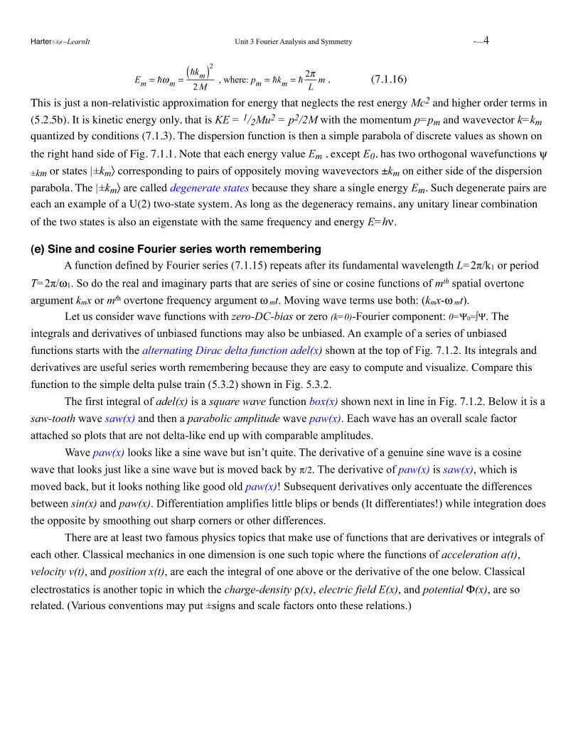
(e) Sine and cosine Fourier series worth remembering A function defined by Fourier series (7.1.15) repeats after its fundamental wavelength L=2π/k1 or period T=2π/ω1. So do the real and imaginary parts that are series of sine or cosine functions of mth spatial overtone argument kmx or mth overtone frequency argument ω mt. Moving wave terms use both: (kmx-ω mt). Let us consider wave functions with zero-DC-bias or zero (k=0)-Fourier component: 0=Ψ0=∫Ψ. The integrals and derivatives of unbiased functions may also be unbiased. An example of a series of unbiased functions starts with the alternating Dirac delta function adel(x) shown at the top of Fig. 7.1.2. Its integrals and derivatives are useful series worth remembering because they are easy to compute and visualize. Compare this function to the simple delta pulse train (5.3.2) shown in Fig. 5.3.2. The first integral of adel(x) is a square wave function box(x) shown next in line in Fig. 7.1.2. Below it is a saw-tooth wave saw(x) and then a parabolic amplitude wave paw(x). Each wave has an overall scale factor attached so plots that are not delta-like end up with comparable amplitudes.
Wave paw(x) looks like a sine wave but isn’t quite. The derivative of a genuine sine wave is a cosine wave that looks just like a sine wave but is moved back by π/2. The derivative of paw(x) is saw(x), which is moved back, but it looks nothing like good old paw(x)! Subsequent derivatives only accentuate the differences between sin(x) and paw(x). Differentiation amplifies little blips or bends (It differentiates!) while integration does the opposite by smoothing out sharp corners or other differences.
There are at least two famous physics topics that make use of functions that are derivatives or integrals of each other. Classical mechanics in one dimension is one such topic where the functions of acceleration a(t), velocity v(t), and position x(t), are each the integral of one above or the derivative of the one below. Classical electrostatics is another topic in which the charge-density ρ(x), electric field E(x), and potential Φ(x), are so related. (Various conventions may put ±signs and scale factors onto these relations.)
HarterSoft –LearnIt Unit 3 Fourier Analysis and Symmetry ----4
5
box(x)
saw(x)
paw(x)
adel(x)
Fig. 7.1.2 Fourier series sharing simple integral or derivative relations to each other.
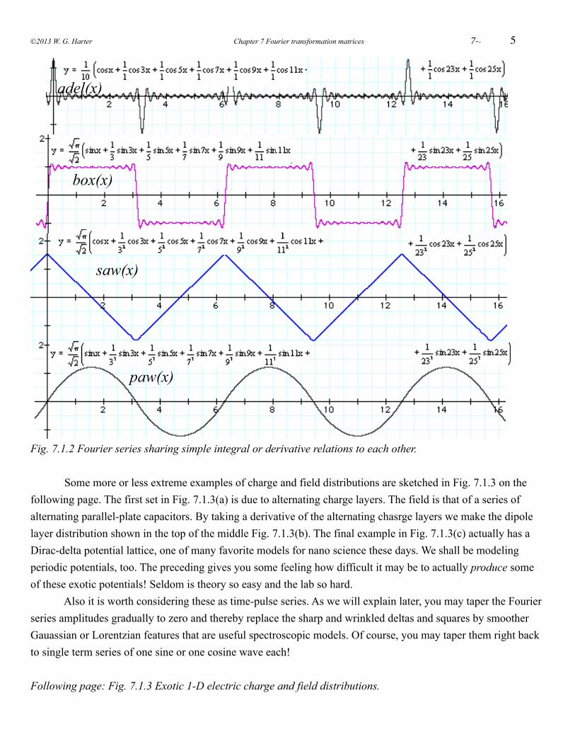
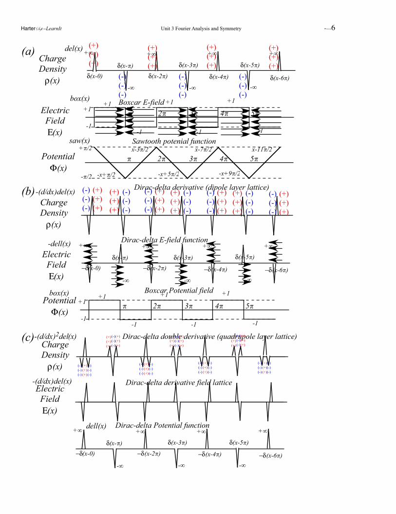
Some more or less extreme examples of charge and field distributions are sketched in Fig. 7.1.3 on the following page. The first set in Fig. 7.1.3(a) is due to alternating charge layers. The field is that of a series of alternating parallel-plate capacitors. By taking a derivative of the alternating chasrge layers we make the dipole layer distribution shown in the top of the middle Fig. 7.1.3(b). The final example in Fig. 7.1.3(c) actually has a Dirac-delta potential lattice, one of many favorite models for nano science these days. We shall be modeling periodic potentials, too. The preceding gives you some feeling how difficult it may be to actually produce some of these exotic potentials! Seldom is theory so easy and the lab so hard. Also it is worth considering these as time-pulse series. As we will explain later, you may taper the Fourier series amplitudes gradually to zero and thereby replace the sharp and wrinkled deltas and squares by smoother Gauassian or Lorentzian features that are useful spectroscopic models. Of course, you may taper them right back to single term series of one sine or one cosine wave each!
Following page: Fig. 7.1.3 Exotic 1-D electric charge and field distributions.
©2013 W. G. Harter Chapter 7 Fourier transformation matrices ! 7--
box(x)
! 2! 3! 4! 5!Boxcar E-field +1 +1
-1 -1
+1
-1
+1
-1
saw(x)
! 2! 3! 4! 5!
Sawtooth potenial function
-x+!/2
x-3!/2+!/2
-!/2 -x+5!/2 -x+9!/2
x-7!/2 x-11!/2
del(x) +∞
δ(x-0) δ(x-2!) δ(x-4!) δ(x-6!)
δ(x-!) δ(x-3!) δ(x-5!)
+∞ +∞ +∞
-∞ -∞ -∞(-)(-)(-)
(+)(+)(+)
(+)(+)(+)
(+)(+)(+)
(+)(+)(+)
(-)(-)(-)
(-)(-)(-)
PotentialΦ(x)
ElectricFieldΕ(x)
ChargeDensityρ(x)
(a)
box(x)
! 2! 3! 4! 5!
Boxcar Potential field+1 +1
-1 -1
+1
-1
+1
-1
-dell(x) Dirac-delta E-field function+∞
−δ(x-0) −δ(x-2!) −δ(x-4!) −δ(x-6!)
δ(x-!) δ(x-3!) δ(x-5!)
+∞ +∞ +∞
-∞ -∞ -∞
(-)(-)(-)
(+)(+)(+)
(+)(+)(+)
(-)(-)(-)
(+)(+)(+)
(-)(-)(-)
(+)(+)(+)
(-)(-)(-)
(-)(-)(-)
(+)(+)(+)
(-)(-)(-)
(+)(+)(+)
(-)(-)(-)
(+)(+)(+)
-(d/dx)del(x) Dirac-delta derivative (dipole layer lattice)
PotentialΦ(x)
ElectricFieldΕ(x)
ChargeDensityρ(x)
(b)
dell(x) Dirac-delta Potential function+∞
−δ(x-0) −δ(x-2") −δ(x-4") −δ(x-6")
δ(x-") δ(x-3") δ(x-5")
+∞ +∞ +∞
-∞ -∞ -∞
-(d/dx)del(x) Dirac-delta derivative field latticeElectricFieldΕ(x)
(-)(-)(-)
(+)(+)(+)
(-)(-)(-)
-(d/dx)2del(x)ChargeDensityρ(x)
Dirac-delta double derivative (quadrupole layer lattice)(-)(-)(-)
(+)(+)(+)
(+)(+)(+)
(-)(-)(-)
(+)(+)(+)
(-)(-)(-)
(-)(-)(-)
(+)(+)(+)
(-)(-)(-)
(-)(-)(-)
(+)(+)(+)
(-)(-)(-)
(-)(-)(-)
(+)(+)(+)
(+)(+)(+)
(-)(-)(-)
(+)(+)(+)
(+)(+)(+)
(c)
HarterSoft –LearnIt Unit 3 Fourier Analysis and Symmetry ----6
7
7.2 Continuous and unbounded x. Continuous and unbounded k! In the preceding cases all wavevectors are restricted by the quantization condition (7.1.3).
! ! ! km = 2π
Lm , where: m = 0,±1, ± 2, ± 3,....± ∞ ! ! ! (7.1.3)repeated
If you let the "cage" become infinitely large ( L → ∞ ) then the wavevector set becomes finer and finer and approaches a continuum. The trick is to replace each sum over index m by an integral over a continuous k-value. If it is done right the wave functions will take a continuous form in both x and k.
! ! ! ! ψ k (x) = x k = ei kx
norm.,!! ! ! ! (7.2.1a)
We need to verify k-orthonormality relations based on wavevector Dirac-delta δ(k′,k)-functions.! !
k ' k = δ k '− k( ) = dx−∞
∞∫ k ' x x k = dx−∞∞∫ ψ k ' (x)*ψ k (x) ,! ! (7.2.1b)
We also need the usual x-completeness relations based on spatial Dirac-delta δ(x′,x)-functions. ! !
x ' x = δ x '− x( ) = dk−∞
∞∫ x ' k k x = dk−∞∞∫ ψ k (x ')*ψ k (x) ! ! (7.2.1c)
! It seems that orthonormality and completeness relations are two sides of the same coin. Orthonormality (7.2.1b) for the k-states { |k〉...|k' 〉..} expresses completeness for the x-states |x〉 , and completeness (7.2.1c) of the k-states |k〉 expresses orthonormality for the x-states { |x〉...|x' 〉..}.! The Dirac notation is extremely efficient but can be confusing. There is a world of difference between the states { |k〉...|k' 〉..} of perfectly monochromatic plane waves and the Dirac position states {|x〉...|x' 〉..} of perfectly localized particles. Recall that we said that an |x〉 state was physically unrealizable; crushing a particle into a single position-x would cost infinite energy. Technically, a |k〉 state is unrealizable, too, since it requires an infinite amount of real estate; we have to let its cage dimension L be infinite, but that seems easier than the extreme solitary confinement needed to make an |x〉 state. If space is cheaper than energy, then |k〉 is easier to approach than |x〉. Lasers easily make approximate |k〉's by being stable and coherent, but producing approximate |x〉's for extremely short pulses requires more difficult engineering.! Use caution to not abuse this notation, though it is easily done. It should be obvious why the following rendition of (7.2.1a) is a dreadful mistake.
! ! !
k k = ei kk
norm.= ei k2
norm. (Dirac abuse. Very BAD mistake!)
Letters x and k denote very different bases which must not to be confused.
(a) Fourier integral transforms
! To achieve the limit of infinite real estate ( L → ∞ ) we replace sums over km = 2π
Lm such as
! ! S =
m=−∞
m=+∞∑ Φk m
= Δmm=−∞
m=+∞∑ Φk m
, where: Δm = 1 !.! ! (7.2.2)
Integrals over k with differential Δkm = 2π
LΔm = 2π
L→ dk or:
ΔmΔkm
= L2π
are used as follows.
©2013 W. G. Harter Chapter 7 Fourier transformation matrices ! 7--
! S = Δm
m=−∞
m=+∞∑ Φk m
= ΔmΔk m
Δk mm=−∞
m=+∞∑ Φk m
becomes → L2π
dk−∞+∞∫ Φ k( ) ! ! (7.2.3)
This, by itself, blows up as we let ( L → ∞ ), but so do the normalization denominators norm. = L , and they cancel. Finally, the Fourier series (7.1.15a) becomes a finite integral.
!
x |Ψ =m=−∞
m=+∞∑
ei k mx
Lkm Ψ becomes → L
2πdk−∞
+∞∫ei k x
Lkm Ψ = dk−∞
+∞∫ei k x
2πL
2πkm Ψ
The trick is to renormalize the k-bases so
L2π
km becomes → k letting the L’s cancel.
! ! !
x |Ψ = dk−∞+∞∫
ei k x
2πk Ψ = dk−∞
+∞∫ x k k Ψ ,! ! ! (7.2.4a)
The newly “normalized” plane wave function ψk(x)=〈x⏐k〉 is defined as follows.
! ! ! !
x k = ei k x
2π! ! ! ! ! ! ! (7.2.4b)
This 〈 x⏐k〉 is the kernal of a Fourier integral transform. An inverse follows by converting (7.1.15b).
!
km Ψ
L=
1L
dx−L / 2
L / 2∫ e−i k mx x Ψ becomes → k Ψ =
L
2πLL
dx−∞
+∞∫ e−i k x x Ψ ,
! ! !
k Ψ = dx−∞
+∞∫
e−i k x
2πx Ψ = dx
−∞
+∞∫ k x x Ψ ,! ! ! (7.2.4c)
Here the inverse kernal 〈k⏐x〉 is simply the conjugate of 〈 x⏐k〉 as required by conjugation axiom-2.
! ! ! !
k x = e−i k x
2π= x k
* .! ! ! ! ! (7.2.4d)
(b) Fourier coefficients: Their many names! The efficiency of the Dirac notation (provided it isn't abused!) should be clear by now. The simple bra-ket 〈x| k〉 stands for so many different mathematical and physical objects. Let's list some.
! (1) 〈x| k〉 is a scalar product of bra 〈x| and ket |k〉 ! (2) 〈x| k〉 is an x-wavefunction for a state |k〉 of definite momentum p = k.! (3) 〈k| x〉=〈x| k〉* is an k-wavefunction for a state |x〉 of definite position x .! (4) 〈x| k〉 is a unitary transformation matrix from position states to momentum states.! (5) 〈x| k〉 is the kernal of a Fourier transform between position states and momentum states.
! As beautiful and compact as it is, the continuum functional Fourier analysis is merely an infinite and unbounded abstraction that lets us use calculus to derive formulas in special cases. Its validity as a limiting case for experimental and numerical analysis should always be questioned. Laboratory and computer experiments, on the other hand, invariably deal with finite and bounded spaces, and it these that we turn to in the next section. We finish this section by relating square-wave Fourier transforms to square-wave Fourier series of the preceding section to help clarify discrete-vs.-continuum relations.
HarterSoft –LearnIt Unit 3 Fourier Analysis and Symmetry ----8
9
(c) Time: Fourier transforms worth remembering! Fourier time-frequency (time-per-time) transforms resemble space-k-vector (space-per-space) transforms (7.2.4). But, a negative sign is put in the exponent so the time phasor turns clockwise.
! t |Ψ = dω−∞+∞∫
e−iωt
2πω Ψ = dω−∞
+∞∫ x ω ω Ψ ! (7.2.5a)! t ω =e−iω t
2π(7.2.5b)
! ω Ψ = dt−∞
+∞∫
eiω t
2πt Ψ = dt
−∞
+∞∫ ω t t Ψ ! ! (7.2.5c)! ω t =
eiω t
2π= t ω * !
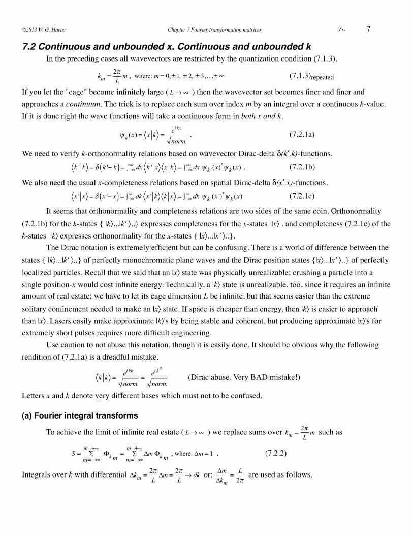
Consider, for example, a single square bump of amplitude B and duration T/2. Its Fourier transform (7.2.5c) is an elementary diffraction function sin ω/ ω that is plotted in Fig. 7.2.1.
! ! ω Ψ = dt−T /4
+T /4∫
eiω t
2πB=B e
iωT /4 − e−iωT /4
iω 2π=2Bsin ωT / 4( )
ω 2π! (7.2.6)
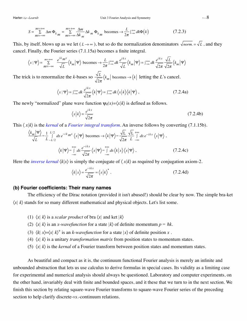
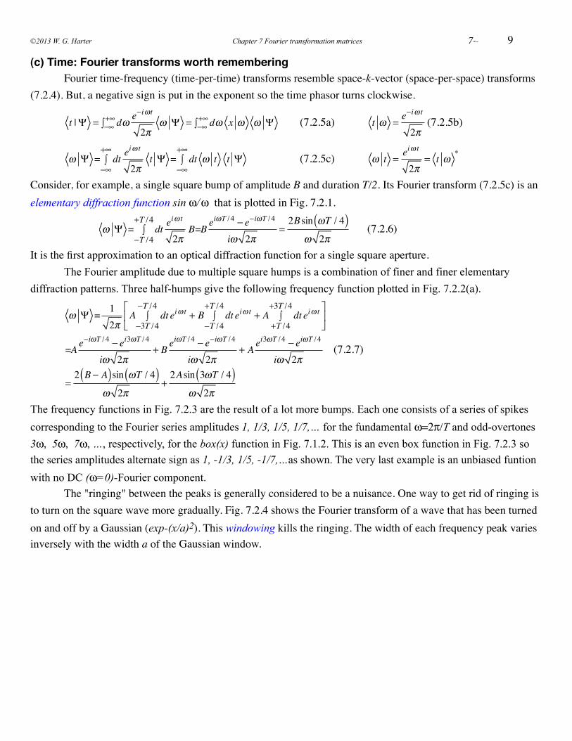
It is the first approximation to an optical diffraction function for a single square aperture. The Fourier amplitude due to multiple square humps is a combination of finer and finer elementary
diffraction patterns. Three half-humps give the following frequency function plotted in Fig. 7.2.2(a).
!
ω Ψ = 12π
A dt−3T /4
−T /4∫ eiω t + B dt
−T /4
+T /4∫ eiω t + A dt
+T /4
+3T /4∫ eiω t
⎡
⎣⎢
⎤
⎦⎥
=A e−iωT /4 − ei3ωT /4
iω 2π+ B e
iωT /4 − e−iωT /4
iω 2π+ A e
i3ωT /4 − eiωT /4
iω 2π
=2 B − A( )sin ωT / 4( )
ω 2π+2Asin 3ωT / 4( )
ω 2π
! (7.2.7)
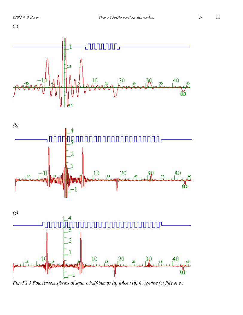
The frequency functions in Fig. 7.2.3 are the result of a lot more bumps. Each one consists of a series of spikes corresponding to the Fourier series amplitudes 1, 1/3, 1/5, 1/7,… for the fundamental ω=2π/T and odd-overtones 3ω, 5ω, 7ω, …, respectively, for the box(x) function in Fig. 7.1.2. This is an even box function in Fig. 7.2.3 so the series amplitudes alternate sign as 1, -1/3, 1/5, -1/7,…as shown. The very last example is an unbiased funtion with no DC (ω=0)-Fourier component.
The "ringing" between the peaks is generally considered to be a nuisance. One way to get rid of ringing is to turn on the square wave more gradually. Fig. 7.2.4 shows the Fourier transform of a wave that has been turned on and off by a Gaussian (exp-(x/a)2). This windowing kills the ringing. The width of each frequency peak varies inversely with the width a of the Gaussian window.
©2013 W. G. Harter Chapter 7 Fourier transformation matrices ! 7--
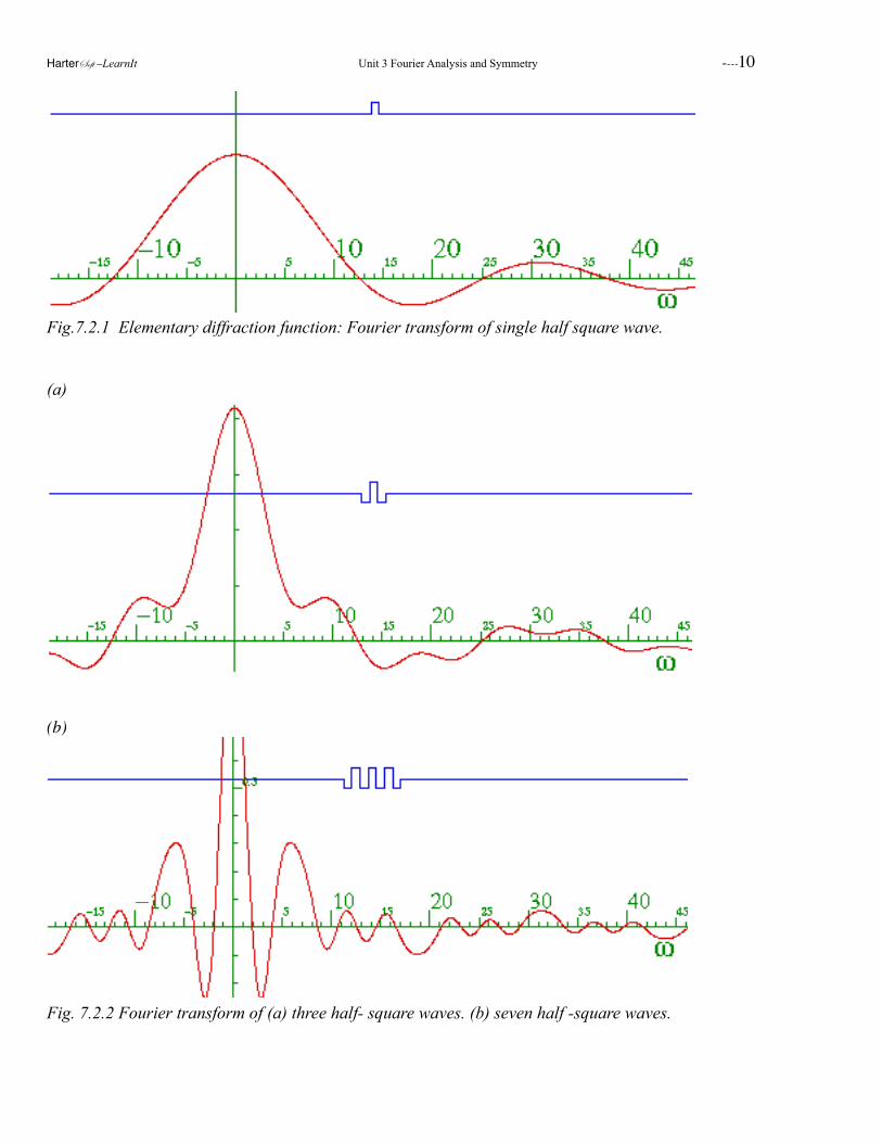
Fig.7.2.1 Elementary diffraction function: Fourier transform of single half square wave.
(a)
(b)
Fig. 7.2.2 Fourier transform of (a) three half- square waves. (b) seven half -square waves.
HarterSoft –LearnIt Unit 3 Fourier Analysis and Symmetry ----10
11
(a)
(b)
(c)
Fig. 7.2.3 Fourier transforms of square half-bumps (a) fifteen (b) forty-nine (c) fifty one .
©2013 W. G. Harter Chapter 7 Fourier transformation matrices ! 7--
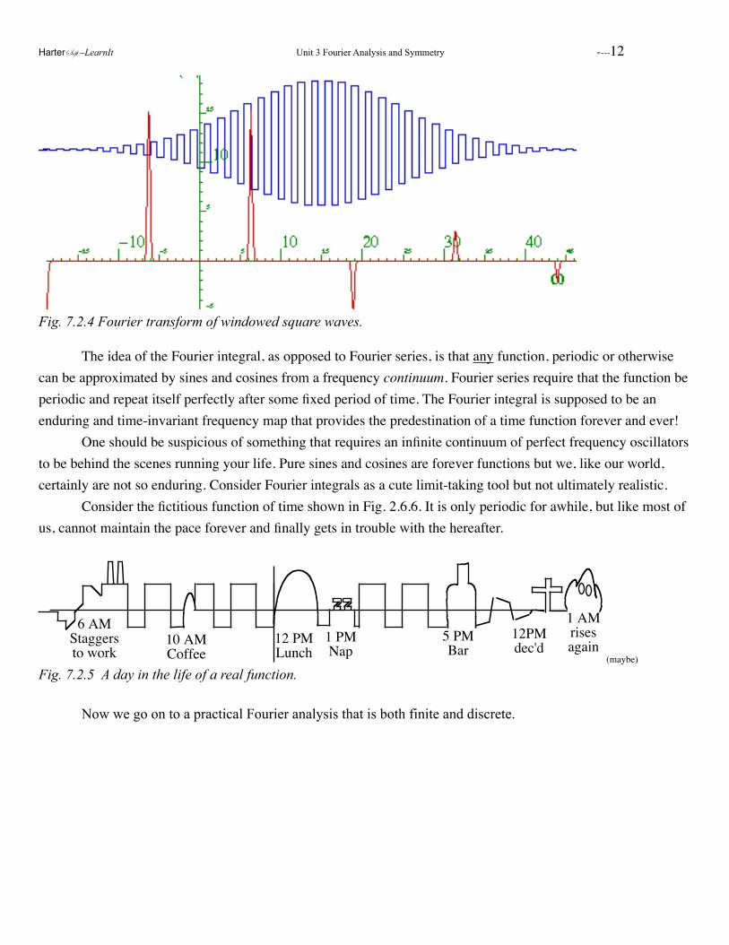
Fig. 7.2.4 Fourier transform of windowed square waves.
! The idea of the Fourier integral, as opposed to Fourier series, is that any function, periodic or otherwise can be approximated by sines and cosines from a frequency continuum. Fourier series require that the function be periodic and repeat itself perfectly after some fixed period of time. The Fourier integral is supposed to be an enduring and time-invariant frequency map that provides the predestination of a time function forever and ever!! One should be suspicious of something that requires an infinite continuum of perfect frequency oscillators to be behind the scenes running your life. Pure sines and cosines are forever functions but we, like our world, certainly are not so enduring. Consider Fourier integrals as a cute limit-taking tool but not ultimately realistic.
Consider the fictitious function of time shown in Fig. 2.6.6. It is only periodic for awhile, but like most of us, cannot maintain the pace forever and finally gets in trouble with the hereafter.
6 AMStaggersto work
10 AMCoffee
12 PMLunch
5 PMBar
12PMdec'd
1 AMrisesagain
1 PMNap
(maybe)
Fig. 7.2.5 A day in the life of a real function.
Now we go on to a practical Fourier analysis that is both finite and discrete.
HarterSoft –LearnIt Unit 3 Fourier Analysis and Symmetry ----12
13
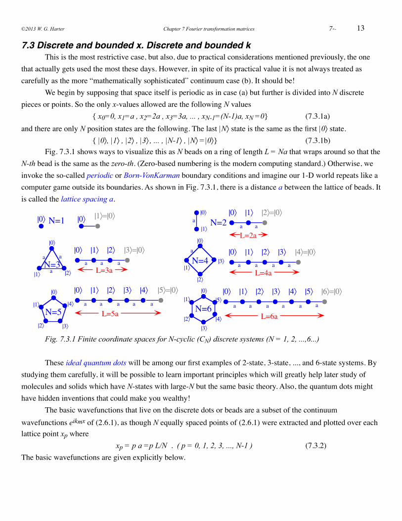
7.3 Discrete and bounded x. Discrete and bounded k! This is the most restrictive case, but also, due to practical considerations mentioned previously, the one that actually gets used the most these days. However, in spite of its practical value it is not always treated as carefully as the more “mathematically sophisticated” continuum case (b). It should be!! We begin by supposing that space itself is periodic as in case (a) but further is divided into N discrete pieces or points. So the only x-values allowed are the following N values ! ! ! { x0=0, x1=a , x2=2a , x3=3a, ... , xN-1=(N-1)a, xN =0}! ! (7.3.1a)and there are only N position states are the following. The last |N〉 state is the same as the first |0〉 state. ! ! ! { |0〉, |1〉 , |2〉 , |3〉 , ... , |N-1〉 , |N〉 =|0〉}! ! ! ! (7.3.1b)! Fig. 7.3.1 shows ways to visualize this as N beads on a ring of length L = Na that wraps around so that the N-th bead is the same as the zero-th. (Zero-based numbering is the modern computing standard.) Otherwise, we invoke the so-called periodic or Born-VonKarman boundary conditions and imagine our 1-D world repeats like a computer game outside its boundaries. As shown in Fig. 7.3.1, there is a distance a between the lattice of beads. It is called the lattice spacing a.
|0〉 |1〉 |2〉 |3〉 |4〉 |5〉 |6〉=|0〉
|0〉 |1〉 |2〉 |3〉 |4〉=|0〉
|0〉 |1〉 |2〉=|0〉
|0〉|1〉
|2〉|3〉
|4〉
|5〉
|0〉
|1〉
|2〉
|3〉
N=6
N=4
|0〉
|1〉N=2
|0〉 |1〉 |2〉 |3〉 |4〉 |5〉=|0〉
|0〉 |1〉 |2〉 |3〉=|0〉
|2〉 |3〉
|4〉
|0〉
|1〉
|0〉
|1〉 |2〉
N=5
N=3
N=1 |0〉 |1〉=|0〉|0〉a
a a
a a a a
a a a
a a a a a
a
a
a
a
aa
a a
a
a
L=3a
L=5a
L=4a
L=6a
L=2a
! Fig. 7.3.1 Finite coordinate spaces for N-cyclic (CN) discrete systems (N = 1, 2, ...,6...)
! These ideal quantum dots will be among our first examples of 2-state, 3-state, ..., and 6-state systems. By studying them carefully, it will be possible to learn important principles which will greatly help later study of molecules and solids which have N-states with large-N but the same basic theory. Also, the quantum dots might have hidden inventions that could make you wealthy!! The basic wavefunctions that live on the discrete dots or beads are a subset of the continuum wavefunctions eikmx of (2.6.1), as though N equally spaced points of (2.6.1) were extracted and plotted over each lattice point xp where! ! ! ! xp = p a =p L/N . ( p = 0, 1, 2, 3, ..., N-1 )! ! ! (7.3.2) The basic wavefunctions are given explicitly below.
©2013 W. G. Harter Chapter 7 Fourier transformation matrices ! 7--
! ! ! ψ km
(xp ) = xp km = ei k mxp
N=ψ km
(xp + L) ! ! ! (7.3.3)
The only change from (7.1.1) is the use of a discrete coordinate xp defined in (7.3.2) above. Also, the normalization constant has been set to the dimension N since all N exponentials eikmx contribute unit magnitude (|eikmx |2 = 1) in the normalization sum.
!
km km =p=0
N −1∑ km xp xp km =
p=0
N −1∑
e−i k mxp
N
ei k mxp
N= N
1N
1N
= 1 ! ! (7.3.4)
! The quantization conditions due to periodicity requirement (7.3.3) over "cage" length L=Na are similar to (7.1.3) but now expressed in terms of the discrete number N and spacing a of lattice points.
! ! ! ei k mL = 1 , or: km = 2π
Lm = 2π
Nam ! ! ! ! (7.3.5a)
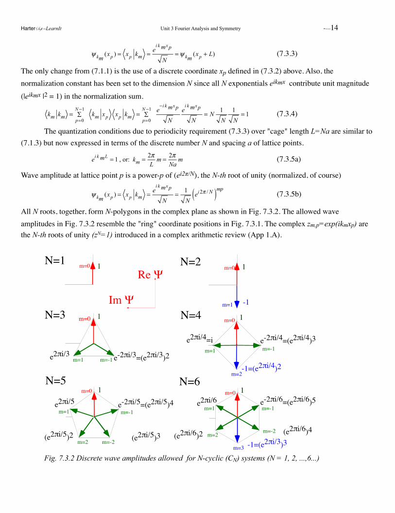
Wave amplitude at lattice point p is a power-p of (ei2π/N), the N-th root of unity (normalized, of course)
! ! ! ψ km
(xp ) = xp km = ei k mxp
N= 1
Nei 2π / N( )mp
! ! ! (7.3.5b)
All N roots, together, form N-polygons in the complex plane as shown in Fig. 7.3.2. The allowed wave amplitudes in Fig. 7.3.2 resemble the "ring" coordinate positions in Fig. 7.3.1. The complex zm,p=exp(ikmxp) are the N-th roots of unity (zN=1) introduced in a complex arithmetic review (App 1.A).
!
N=1
1
e2πi/3 e-2πi/3=(e2πi/3)2
1
N=3
N=2 1
e2πi/4=i
N=4
1
e2πi/5
N=5
1
e2πi/6
N=61
-1
(e2πi/5)2 (e2πi/5)3
e-2πi/5=(e2πi/5)4
(e2πi/6)2-1=(e2πi/3)3
-1=(e2πi/4)2
e-2πi/4=(e2πi/4)3
(e2πi/6)4
e-2πi/6=(e2πi/6)5
Re Ψ
Im Ψ
m=0
m=0
m=0
m=0
m=0
m=1
m=0
m=1
m=1
m=1
m=1
m=-1
m=-1 m=-1
m=-1
m=-2
m=-2
m=2m=2
m=3
m=2
! Fig. 7.3.2 Discrete wave amplitudes allowed for N-cyclic (CN) systems (N = 1, 2, ...,6...)
HarterSoft –LearnIt Unit 3 Fourier Analysis and Symmetry ----14
15
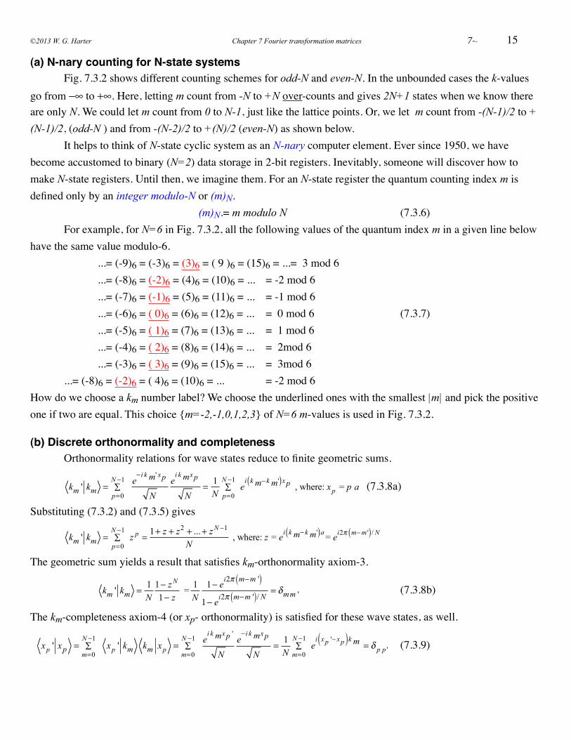
(a) N-nary counting for N-state systems! Fig. 7.3.2 shows different counting schemes for odd-N and even-N. In the unbounded cases the k-values go from −∞ to +∞. Here, letting m count from -N to +N over-counts and gives 2N+1 states when we know there are only N. We could let m count from 0 to N-1, just like the lattice points. Or, we let m count from -(N-1)/2 to +(N-1)/2, (odd-N ) and from -(N-2)/2 to +(N)/2 (even-N) as shown below.! It helps to think of N-state cyclic system as an N-nary computer element. Ever since 1950, we have become accustomed to binary (N=2) data storage in 2-bit registers. Inevitably, someone will discover how to make N-state registers. Until then, we imagine them. For an N-state register the quantum counting index m is defined only by an integer modulo-N or (m)N.! ! ! ! ! (m)N.= m modulo N ! ! ! ! (7.3.6) ! For example, for N=6 in Fig. 7.3.2, all the following values of the quantum index m in a given line below have the same value modulo-6. ! ! ...= (-9)6 = (-3)6 = (3)6 = ( 9 )6 = (15)6 = ...= 3 mod 6! ! ...= (-8)6 = (-2)6 = (4)6 = (10)6 = ... != -2 mod 6! ! ...= (-7)6 = (-1)6 = (5)6 = (11)6 = ... ! = -1 mod 6 ! ! ...= (-6)6 = ( 0)6 = (6)6 = (12)6 = ... != 0 mod 6! ! ! (7.3.7)! ! ...= (-5)6 = ( 1)6 = (7)6 = (13)6 = ... ! = 1 mod 6!! ! ...= (-4)6 = ( 2)6 = (8)6 = (14)6 = ... ! = 2mod 6!! ! ...= (-3)6 = ( 3)6 = (9)6 = (15)6 = ... ! = 3mod 6! ...= (-8)6 = (-2)6 = ( 4)6 = (10)6 = ... ! ! = -2 mod 6How do we choose a km number label? We choose the underlined ones with the smallest |m| and pick the positive one if two are equal. This choice {m=-2,-1,0,1,2,3} of N=6 m-values is used in Fig. 7.3.2.
(b) Discrete orthonormality and completeness! Orthonormality relations for wave states reduce to finite geometric sums.
!
km ' km =p=0
N −1∑
e−i k m' xp
N
ei k mxp
N= 1
N p=0
N −1∑ e
i k m−k m'( )xp , where: xp = p a !(7.3.8a)
Substituting (7.3.2) and (7.3.5) gives
!
km ' km =p=0
N −1∑ z p = 1+ z + z2 + ...+ z N −1
N , where: z = ei k m−k m'( )a = ei2π m−m '( )/ N
The geometric sum yields a result that satisfies km-orthonormality axiom-3.
! !
km ' km = 1N
1− z N
1− z = 1
N1− ei2π m−m '( )
1− ei2π m−m '( )/ N= δmm ' ! ! ! (7.3.8b)
The km-completeness axiom-4 (or xp- orthonormality) is satisfied for these wave states, as well.
xp ' xp =m=0
N −1∑ xp ' km km xp =
m=0
N −1∑
ei k mxp '
N
e−i k mxp
N= 1
N m=0
N −1∑ e
i xp '− xp( )k m = δ p p ' ! (7.3.9)
©2013 W. G. Harter Chapter 7 Fourier transformation matrices ! 7--
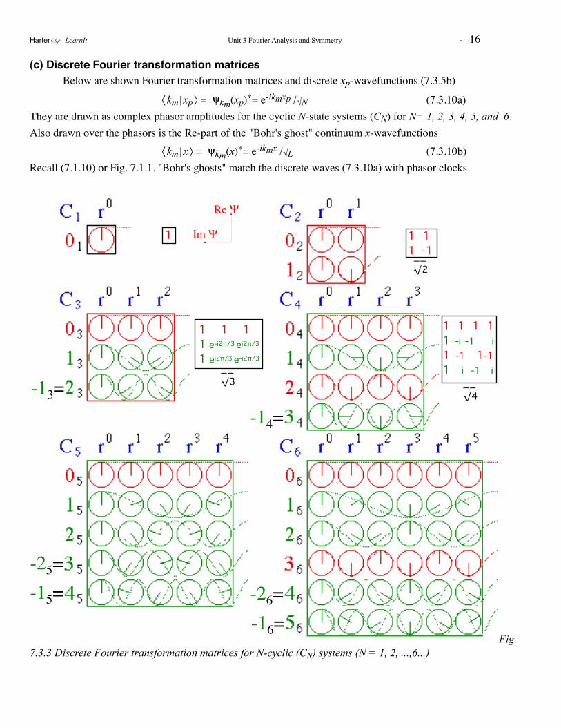
(c) Discrete Fourier transformation matrices! Below are shown Fourier transformation matrices and discrete xp-wavefunctions (7.3.5b)
! ! ! ! 〈 km | xp 〉 = ψkm(xp)*= e-ikmxp /√N ! ! ! ! (7.3.10a)!They are drawn as complex phasor amplitudes for the cyclic N-state systems (CN) for N= 1, 2, 3, 4, 5, and 6. Also drawn over the phasors is the Re-part of the "Bohr's ghost" continuum x-wavefunctions! ! ! ! 〈 km | x 〉 = ψkm(x)*= e-ikmx /√L ! ! ! ! (7.3.10b)!Recall (7.1.10) or Fig. 7.1.1. "Bohr's ghosts" match the discrete waves (7.3.10a) with phasor clocks.
1 1 11 -1
1 1 11 e-i2π/3 ei2π/3
1 ei2π/3 e-i2π/3
1 1 1 11 -i -1 i1 -1 1-11 i -1 i
__√2
__√3 __
√4
-16=-26=
-25=-15=
-14=-13=
Re Ψ
Im Ψ
Fig. 7.3.3 Discrete Fourier transformation matrices for N-cyclic (CN) systems (N = 1, 2, ...,6...)
HarterSoft –LearnIt Unit 3 Fourier Analysis and Symmetry ----16
17
(d) Intoducing aliases and Brillouin zones! It is important to see the relation between the continuum waves and their "course-grained" images thatves with integral wave-numbers of m mod N whole wavelengths within each 〈 km |-row of phasors. We might as well call them "row-waves" or "bra-waves." Note also, that the same wave shape exists in the columns or kets | xp 〉. Each “ket-wave” | xp 〉 represents a δ-position state or “pulse” localized at point xp . The inverse Fourier transformation 〈 km | xp 〉 relates | xp 〉 to a bra-wave〈 km |. As required by conjugation axiom-2, namely, 〈 km | xp 〉=
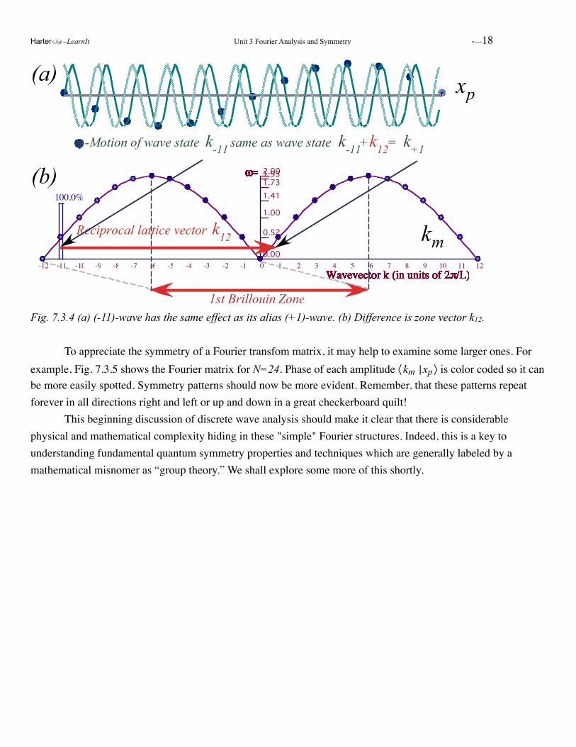
〈 xp | km 〉∗, the relation is the same as between | km 〉 and 〈 xp | , except for conjugation.! For low wave number like, say (mN )=(1)6 or (2)6, it is easy to see the "Bohr's-ghost wave" mirrored in the phasors as in the second and third row of the C6 matrix in Fig. 7.3.1. Note however, that these phasors are set so the phase of the one to the right is clockwise (that is it appears ahead) of the one to the left. This means, if the phasors turned clockwise, that the one to the right is feeding energy into the one to its left, so the wave would be moving right-to-left with wave momentum minus (1)6 or minus (2)6, respectively. But, they're conjugated bras so their clocks go backwards and so the labels are OK, after all.! For high wave number like, say (mN )=(4)6 or (5)6, it is not so easy to see the "Bohr's-ghost wave" mirrored in the phasors as in the fifth and sixth row of the C6 matrix in Fig. 7.3.1. But, you can see alias waves of negative wave momentum (mN )=(-2)6 or (-1)6 , respectively, that is oppositely moving waves of low wavenumber. Recall that (4 mod 6) equals (-2 mod 6) and (5 mod 6) equals (-1 mod 6).! Right in the middle row of the even-N matrix is a wave that isn't going in either direction. In the C6 matrix it is the (3)6 wave. Since (3 mod 6) equals (-3 mod 6) this is a good old push-me-pull-you standing wave with all real amplitudes of (1, -1, 1, -1, 1, -1). This can only happen for even-N and is known as a first Brillouin zone boundary wave in solid-state physics. ! All cases have a zero-momentum wave (0N ) at the top of the transformation matrix. This is called the Brillouin zone center wave in solid-state physics. Indeed, it is centered at the bottom of the dispersion plot in Fig. 2.6.1. Its phasor settings are the same as that of a higher (NN ), or (2NN ), or (3NN ), ...etc. wave. However, this N-state system does not count higher than N-1 without recycling.! Consider, for example, a k-11 wave of wavevector (-11)12 (with minus-eleven-kinks-modulo-12) as plotted in Fig. 7.3.4 (a). Since (–11)-mod-12 equals (+1)-mod-12 (that is, (-11)12=(+1)12) it follows that the wave shown has the same effect as a (+1)12 wave. Indeed, the twelve masses in Fig. 7.3.4(a) line up on a single-kink (k=1)-wave moving positively, while the (k=-11)-wave moves negatively. (See WaveIt movie.) This is an example of aliasing. In a C12 lattice, (k=-11) is an alias for (k=+1). ! Fig. 7.3.4(b) shows the k-space with a typical frequency dispersion function plotted above it. The difference between any two alias wavevectors such as (k=+1) and (k=-11) is a reciprocal lattice vector k12 or (12)12=(0)12. The reciprocal lattice vector k12 also spans the first Brillouin-zone from (-6)12 to (+6)12 as shown at the bottom of the figure. An important idea here is that a wavevector k-space must have the same N-fold periodic symmetry as the coordinate x-space. Moving across row of a 〈 km | xp 〉 matrix gives the same variation as moving up the corresponding column since 〈 km | xp 〉 is unitary. Both are N-fold periodic!
©2013 W. G. Harter Chapter 7 Fourier transformation matrices ! 7--
xp
-Motion of wave state k-11 same as wave state k-11+k12= k+1
(a)
-12Wavevector k (in units of 2π/L)Wavevector k (in units of 2π/L)Wavevector k (in units of 2π/L)Wavevector k (in units of 2π/L)Wavevector k (in units of 2π/L)Wavevector k (in units of 2π/L)Wavevector k (in units of 2π/L)Wavevector k (in units of 2π/L)Wavevector k (in units of 2π/L)Wavevector k (in units of 2π/L)Wavevector k (in units of 2π/L)Wavevector k (in units of 2π/L)Wavevector k (in units of 2π/L)Wavevector k (in units of 2π/L)Wavevector k (in units of 2π/L)Wavevector k (in units of 2π/L)Wavevector k (in units of 2π/L)Wavevector k (in units of 2π/L)Wavevector k (in units of 2π/L)Wavevector k (in units of 2π/L)Wavevector k (in units of 2π/L)Wavevector k (in units of 2π/L)Wavevector k (in units of 2π/L)Wavevector k (in units of 2π/L)Wavevector k (in units of 2π/L)
ω=
-11
ω=
100.0%
-10
ω=
-9
ω=
-8
ω=
-7
ω=
-6
ω=
-5
ω=
-4
ω=
-3
ω=
-2
ω=
-1
ω=
00.00
ω=
1
0.52
ω=
2
1.00
ω=
3
1.41
ω=
4
1.73ω=
5
1.93ω=
6
2.00ω=
7
ω=
8
ω=
9
ω=
10
ω=
11
ω=
12
ω=
kmReciprocal lattice vector k12
1st Brillouin Zone
(b)
Fig. 7.3.4 (a) (-11)-wave has the same effect as its alias (+1)-wave. (b) Difference is zone vector k12.
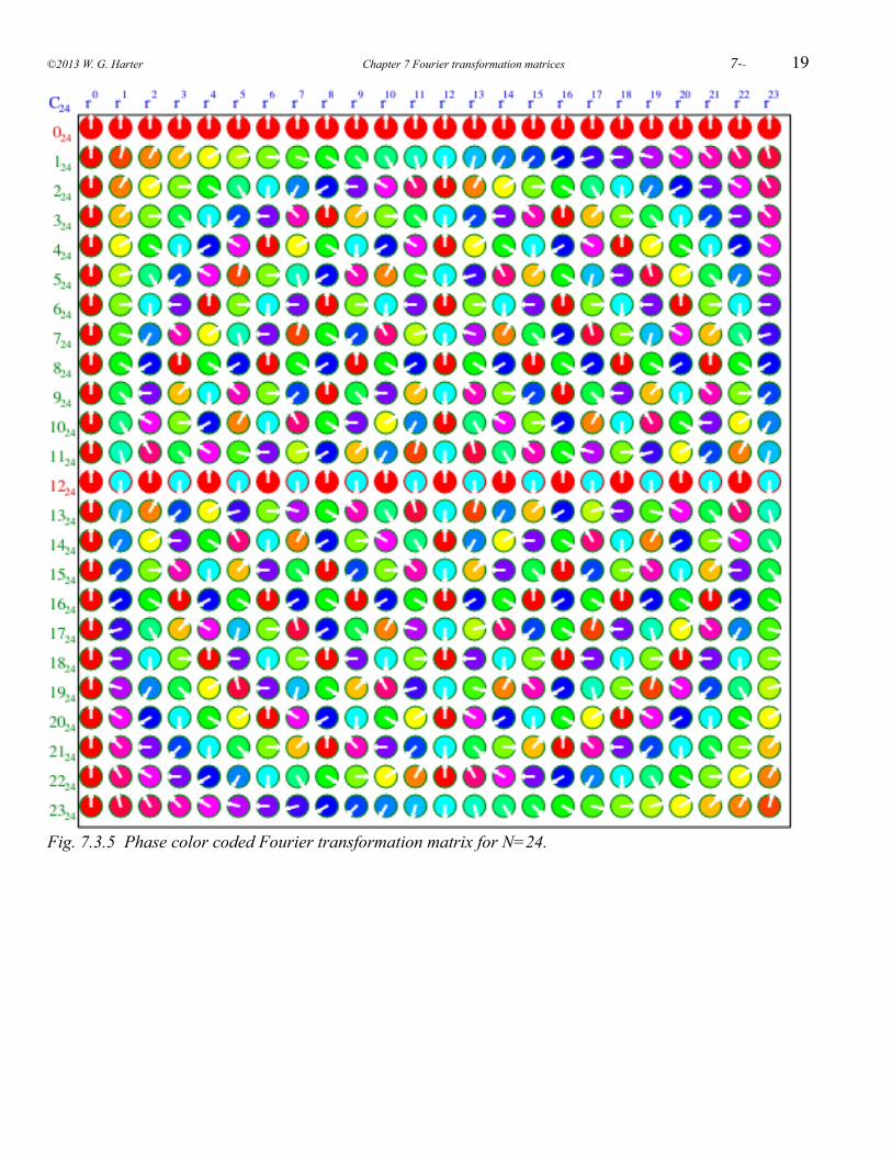
! To appreciate the symmetry of a Fourier transfom matrix, it may help to examine some larger ones. For example, Fig. 7.3.5 shows the Fourier matrix for N=24. Phase of each amplitude 〈 km | xp 〉 is color coded so it can be more easily spotted. Symmetry patterns should now be more evident. Remember, that these patterns repeat forever in all directions right and left or up and down in a great checkerboard quilt!! This beginning discussion of discrete wave analysis should make it clear that there is considerable physical and mathematical complexity hiding in these "simple" Fourier structures. Indeed, this is a key to understanding fundamental quantum symmetry properties and techniques which are generally labeled by a mathematical misnomer as “group theory.” We shall explore some more of this shortly.
HarterSoft –LearnIt Unit 3 Fourier Analysis and Symmetry ----18
19
Fig. 7.3.5 Phase color coded Fourier transformation matrix for N=24.
©2013 W. G. Harter Chapter 7 Fourier transformation matrices ! 7--
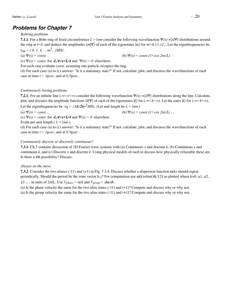
Problems for Chapter 7Bohring problems7.1.1. For a Bohr ring of fixed circumference L =1nm consider the following wavefunction Ψ(x) =〈x|Ψ〉 distributions around the ring at t=0, and deduce the amplitudes 〈m|Ψ〉 of each of the eigenstates |m〉 for m=0,±1,±2,.. Let the eigenfrequencies be νm = ( 0, 1, 4, . , m2, .)MHz. (a) Ψ(x) = const. . ! ! ! ! ! ! (b) Ψ(x) = const.(1+cos 2πx/L) .(c) Ψ(x) = const. for -L/4<x<L/4 and Ψ(x) = 0 elsewhere.For each case evaluate const. assuming one particle occupies the ring. (d) For each case (a) to (c) answer: "Is it a stationary state?" If not, calculate, plot, and discusss the wavefunctions of each case at time t = 1µsec, and at 0.5µsec .
Continuously boring problems7.2.1. For an infinite line (-∞<x<∞) consider the following wavefunction Ψ(x) =〈x|Ψ〉 distributions along the line. Calculate, plot, and discusss the amplitude functions 〈k|Ψ〉 of each of the eigenstates |k〉 for (-∞<k<∞). Let the eates |k〉 for (-∞<k<∞). Let the eigenfrequencies be νk = ( kL/2π)2MHz. (Let unit length be L =1nm.)(a) Ψ(x) = const. . ! ! ! ! ! ! (b) Ψ(x) = const.(1+cos 2πx/L) . .(c) Ψ(x) = const. for -L/4<x<L/4 and Ψ(x) = 0 elsewhere.Evalu per unit length ( L =1nm.). (d) For each case (a) to (c) answer: "Is it a stationary state?" If not, calculate, plot, and discusss the wavefunctions of each case at time t = 1µsec, and at 0.5µsec .
Continuously discrete or discretely continuous?7.3.1. Ch.7 contains discussion of 1D Fourier wave systems with (a) Continuous x and discrete k, (b) Continuous x and continuous k, and (c) Discrete x and discrete k. Using physical models of each to discuss how physically relizeable these are. Is there a 4th possibility? Discuss.
Aliases on the move7.3.2. Consider the two aliases (-11) and (+1) in Fig. 7.3.4. Discuss whether a dispersion function ω(k) should repeat periodically. Should the period be the zone vector k12? For computation use ω(k)=|sin(πk/12)| as plotted where k=0, ±1, ±2, ±3 ,… in units of 2π/L. Use Vphase = ω/k and Vgroup = dω/dk .(a) Is the phase velocity the same for the two alias states (-11) and (+1)? Compute and discuss why or why not.(a) Is the group velocity the same for the two alias states (-11) and (+1)? Compute and discuss why or why not.
HarterSoft –LearnIt Unit 3 Fourier Analysis and Symmetry ----20
1
QMfor
AMOPΨ
Chapter 8Fourier Symmetry Analysis
W. G. Harter
©2013 W. G. Harter Chapter 8. Fourier Symmetry ! 8--
........................................................................CHAPTER 8. FOURIER SYMMETRY ANALYSIS ! 3
8.1. Introducing Cyclic Symmetry: A C6 ....................................................................................................................... example! 3(a) Cyclic symmetry CN ..................................................................................................................: A 6-quantum-dot analyzer! 3(b) CN ............................................................................................................................ Symmetry groups and representations! 5
.........................................................................................................................................(c) So what’s a group representation?! 6
8.2 CN Spectral Decomposition: Solving a C6 .................................................................................................. transfer matrix! 7(a) Spectral decomposition of symmetry operators rp.................................................................................................................! 7(b) Writing transfer operator T in terms of symmetry operators rp .............................................................................................! 9
....................................................................................................................(c) Spectral decomposition of transfer operator T! 10An eigenvalue formula for all possible C6 ........................................................................................ symmetric T-matrices! 10What do the km .................................................................................................................................- eigensolutions mean?! 11
(d) OK, where did those eikx ........................................................................................................ wavefunctions come from?! 12
.................................................................................................................................8.3 Related Symmetry Analysis Examples! 13(a) Dihedral symmetry D2 .........................................................................................................................................................! 14
D2 ................................................................................................................................................................. group structure! 14D2 ..................................................................................................... spectral decomposition: The old “1=1•1 trick” again! 15Spectral decomposition of D2 ................................................................................................................... transfer matrices! 15
..................................................................................................................(b) Outer product structure: Double qubit registers! 16D2 is product C2×C2..............................................................................................................................................................! 16
...........................................................................................................................................Big-endian versus Little-endian! 17C6 is product C3× C2 (but C4 is NOT C2× C2 ......................................................................................................................)! 17
................................................................................................................................................................Symmetry Catalog! 17
..............................................................................................................................................................Problems for Chapter 8.! 18
Fourier analysis is most useful when there is a symmetry G in which all the coordinate points are indistinguishable. For an unbounded x-continuum, G is an infinite translational symmetry group labeled T. For a bounded xp-ring of “quantum dots” the symmetry G is an N-cyclic rotation group labeled CN. In Chapter 8 a fictitious hexagonal beam analyzer with C6 symmetry is considered. The transfer matrix eigensolutions of such a device are found using a modern form of Fourier analysis known as group representation theory or symmetry analysis, one of the most powerful tools in quantum theory. The symmetry of the bounded Bohr x-ring continuum is also discussed.
HarterSoft –LearnIt Unit 3 Fourier Analysis and Symmetry ----2
3
Chapter 8. Fourier Symmetry Analysis From where do the wavefunctions like Ψ = ei(kx - ωt) come? One answer to this involves the concept of symmetry analysis and group representation theory. These sound like big names for what is still regarded as a pretty scary mathematical subject. However, the basic ideas of this powerful tool are actually quite simple as we hope to show now. Most of the needed algebraic work has been done in Ch. 3 regarding spectral decomposition. The physical ideas of Fourier analysis and Bohr ring waves are in Ch. 7. Symmetry group representation theory is really just a beautiful generalization of Fourier analysis that gives eigensolutions of “difficult” operators using simple properties of commuting symmetry operators.
8.1. Introducing Cyclic Symmetry: A C6 example A ring of quantum dots was introduced in Section 7.3 as a model for finite Fourier analysis. The Fourier tranformation matrix was discussed with examples for N=1, 2, 3, 4, 5, and 6. The idea of cyclic symmetry CN was broached as a property of the matrices in Fig. 7.3.3 and Fig. 7.3.5. Here that idea is put on a more solid footing.
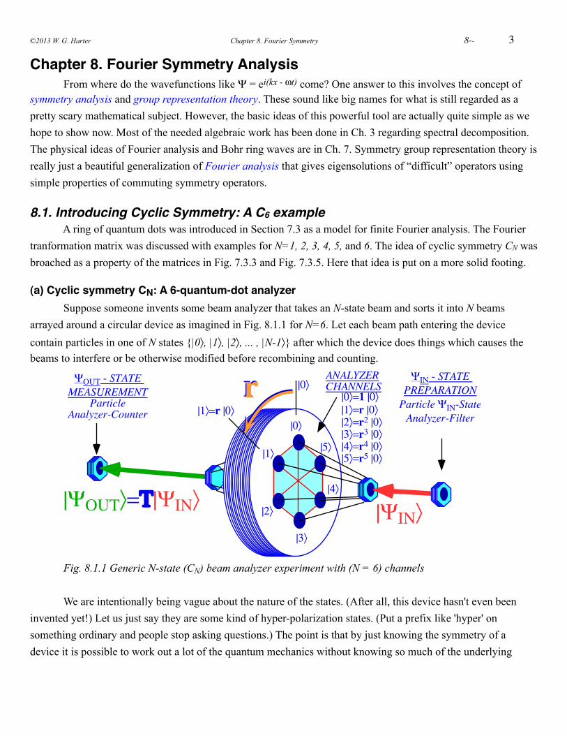
(a) Cyclic symmetry CN: A 6-quantum-dot analyzer Suppose someone invents some beam analyzer that takes an N-state beam and sorts it into N beams arrayed around a circular device as imagined in Fig. 8.1.1 for N=6. Let each beam path entering the device contain particles in one of N states {|0〉, |1〉, |2〉, ... , |N-1〉} after which the device does things which causes the beams to interfere or be otherwise modified before recombining and counting.
!
|0〉|1〉=r |0〉|2〉=r2 |0〉
|4〉=r4 |0〉|5〉=r5 |0〉
|0〉=1 |0〉
|3〉=r3 |0〉
|2〉
|3〉
|4〉
|5〉|1〉
rr|1〉=r |0〉
|0〉
|ΨIN〉|ΨOUT〉=ΤΤ|ΨIN〉
ΨIN - STATEPREPARATIONParticle ΨIN-StateAnalyzer-Filter
ANALYZERCHANNELS
ΨOUT - STATEMEASUREMENT
ParticleAnalyzer-Counter
Fig. 8.1.1 Generic N-state (CN) beam analyzer experiment with (N = 6) channels
We are intentionally being vague about the nature of the states. (After all, this device hasn't even been invented yet!) Let us just say they are some kind of hyper-polarization states. (Put a prefix like 'hyper' on something ordinary and people stop asking questions.) The point is that by just knowing the symmetry of a device it is possible to work out a lot of the quantum mechanics without knowing so much of the underlying
©2013 W. G. Harter Chapter 8. Fourier Symmetry ! 8--
details. It is a lot like the photon polarization and electron spin problems discussed in Chapter 1. Electron and photon “spin” are physically quite different but use much of the same mathematical theory. By symmetry, we mean any operators r, r2,.. that do not alter the analyzer experiment no matter how many times you apply them. In particular, suppose a 60° rotational operator r indicated in Fig. 8.1.1. could be done some night by the lab janitor, so when the physicists show up the next morning all their experiments work the same as the day before. However, it is important to state what we mean the janitor's r-operation to do. He could just rotate the whole lab building by 60°. That, indeed, is a symmetry, but not one we will discuss until later. Besides, a rotation like that happens every four hours as the Earth turns; no janitor needed! This is called the symmetry of isotropy of space. It is a continuous or Lie symmetry for which 60° has no special significance. Instead, what we have in mind for the janitor to do is rotate just the analyzer in the center of Fig. 8.1.1 by 60° as indicated in the figure. Well, that analyzer looks pretty heavy, so, instead we'll ask that the janitor just rotate the little input source and the little output counter both by minus 60°, which is operation r -1=r 5. This does the same as a whole-Earth/lab rotation by -60° (which no one detects) followed by a positive 60° rotation of the big analyzer to "upright" leaving input and output devices behind at -60°. It is important to understand that all transformations are relative transformations; something gets moved or mapped relative to something else. You've probably heard it quoted, "Everything's relative!" Well, that's often garbage, but here it isn't. Rotations, Lorentz transformations, and our analyzer operators T (Recall Fig. 1.6.1), and r in Fig. 8.1.1 are all mappings of one vector or thing relative to another. By the way, our helpful suggestion to the janitor won't help much if the input and output devices are big analyzers, too. It was noted in Chapter 1 that filters and counters are analyzers set in certain ways. But, the analyzer in Fig. 8.1.1 is a more powerful one than heretofore discussed. (And, isn't better always bigger?) So let's assume that the janitor can easily do r -1 = r 5 to the smaller input and output devices whose in and out states are written as follows in Dirac notation, |ΨOUT (r-1)〉 = r -1|ΨOUT〉 , |ΨIN (r-1)〉 = r -1 |ΨIN〉 . (8.1.1) Symmetry of the transformation operator T means it does exactly the same relative thing to any state |ΨIN〉 as it does to the janitor-rotated state |ΨIN (r-1)〉 , that is |ΨOUT〉 = T |ΨIN〉 implies: |ΨOUT (r-1)〉 = T |ΨIN (r-1)〉 (8.1.2a)or r -1|ΨOUT〉 = T r -1|ΨIN〉 (8.1.2b) |ΨOUT〉 = r T r -1|ΨIN〉 (8.1.2c)If this is true for all input states |ΨIN〉 then it follows that effect of analyzer operator T in (8.1.2a) and in (8.1.2c) are indistinguishable, or T is invariant to r T = r T r -1 or: r -1T r = T (8.1.2d)or, that r commutes with T; the latter being the most common way to say that T has r-symmetry. T r = r T (8.1.2e)All the above parts of equation (8.1.2) are really the same requirement for r-symmetry of T.
HarterSoft –LearnIt Unit 3 Fourier Analysis and Symmetry ----4
5
Note: This is not the same as just multiplying both sides of |ΨOUT〉 = T |ΨIN〉 by r or r -1 which just gives a whole-Earth/lab rotation, that is, operate with r -1 and insert the identity (r r -1 =1) to get r -1 |ΨOUT〉 = r -1 T |ΨIN〉 = r -1 T r r -1 |ΨIN〉 . (8.1.3a) This reduces to an expression similar to the original |ΨOUT〉 = T |ΨIN〉 |ΨOUT (r-1)〉 = r -1 T |ΨIN〉 = r -1 T r |ΨIN (r-1)〉 = T (r-1) |ΨIN (r-1)〉 (8.1.3b)where T (r-1) is a similarity transformation r -1T r of T . (This is an active transformation; devices move.) T (r-1) = r -1 T r (8.1.3c)These relations hold true for any analyzer operator T whether it has symmetry or not. For T to have r-symmetry it is necessary that the similarity transformation leaves T unchanged or invariant (T (r-1) = T), as in (8.1.2d).To recap An analyzer has r-symmetry if and only if its operator T commutes with r , that is (T r = r T).
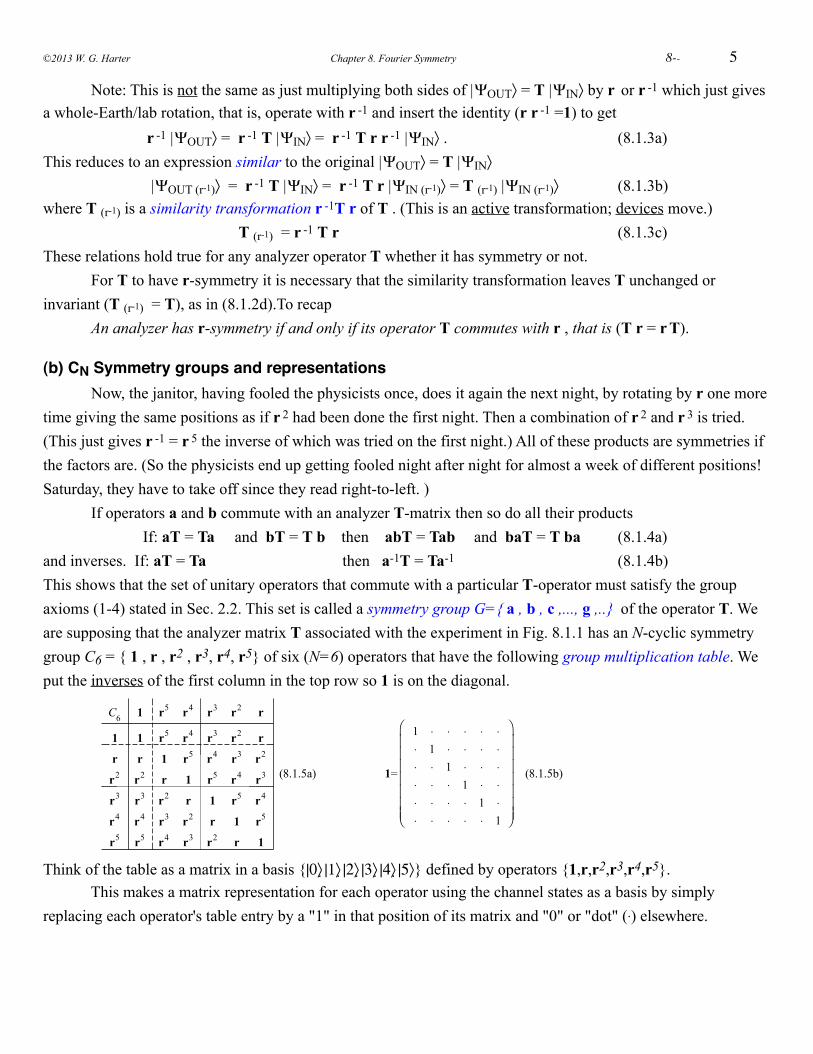
(b) CN Symmetry groups and representations Now, the janitor, having fooled the physicists once, does it again the next night, by rotating by r one more time giving the same positions as if r 2 had been done the first night. Then a combination of r 2 and r 3 is tried. (This just gives r -1 = r 5 the inverse of which was tried on the first night.) All of these products are symmetries if the factors are. (So the physicists end up getting fooled night after night for almost a week of different positions! Saturday, they have to take off since they read right-to-left. ) If operators a and b commute with an analyzer T-matrix then so do all their products If: aT = Ta and bT = T b then abT = Tab and baT = T ba (8.1.4a)and inverses. If: aT = Ta then a-1T = Ta-1 (8.1.4b)This shows that the set of unitary operators that commute with a particular T-operator must satisfy the group axioms (1-4) stated in Sec. 2.2. This set is called a symmetry group G={ a , b , c ,..., g ,..} of the operator T. We are supposing that the analyzer matrix T associated with the experiment in Fig. 8.1.1 has an N-cyclic symmetry group C6 = { 1 , r , r2 , r3, r4, r5} of six (N=6) operators that have the following group multiplication table. We put the inverses of the first column in the top row so 1 is on the diagonal.
C6 1 r5 r4 r3 r2 r
1 1 r5 r4 r3 r2 r
r r 1 r5 r4 r3 r2
r2 r2 r 1 r5 r4 r3
r3 r3 r2 r 1 r5 r4
r4 r4 r3 r2 r 1 r5
r5 r5 r4 r3 r2 r 1
(8.1.5a) 1=
1 ⋅ ⋅ ⋅ ⋅ ⋅⋅ 1 ⋅ ⋅ ⋅ ⋅⋅ ⋅ 1 ⋅ ⋅ ⋅⋅ ⋅ ⋅ 1 ⋅ ⋅⋅ ⋅ ⋅ ⋅ 1 ⋅⋅ ⋅ ⋅ ⋅ ⋅ 1
⎛
⎝
⎜⎜⎜⎜⎜⎜⎜
⎞
⎠
⎟⎟⎟⎟⎟⎟⎟
(8.1.5b)
Think of the table as a matrix in a basis {|0〉 |1〉 |2〉 |3〉 |4〉 |5〉} defined by operators {1,r,r2,r3,r4,r5}. This makes a matrix representation for each operator using the channel states as a basis by simply replacing each operator's table entry by a "1" in that position of its matrix and "0" or "dot" (.) elsewhere.
©2013 W. G. Harter Chapter 8. Fourier Symmetry ! 8--
0 1 2 3 4 5 0 1 2 3 4 5 0 1 2 3 4 5 0 1 2 3 4 5 0 1 2 3 4 5
r=
⋅ ⋅ ⋅ ⋅ ⋅ 11 ⋅ ⋅ ⋅ ⋅ ⋅⋅ 1 ⋅ ⋅ ⋅ ⋅⋅ ⋅ 1 ⋅ ⋅ ⋅⋅ ⋅ ⋅ 1 ⋅ ⋅⋅ ⋅ ⋅ ⋅ 1 ⋅
⎛
⎝
⎜⎜⎜⎜⎜⎜⎜
⎞
⎠
⎟⎟⎟⎟⎟⎟⎟
,r2 =
⋅ ⋅ ⋅ ⋅ 1 ⋅⋅ ⋅ ⋅ ⋅ ⋅ 11 ⋅ ⋅ ⋅ ⋅ ⋅⋅ 1 ⋅ ⋅ ⋅ ⋅⋅ ⋅ 1 ⋅ ⋅ ⋅⋅ ⋅ ⋅ 1 ⋅ ⋅
⎛
⎝
⎜⎜⎜⎜⎜⎜⎜
⎞
⎠
⎟⎟⎟⎟⎟⎟⎟
, r3=
⋅ ⋅ ⋅ 1 ⋅ ⋅⋅ ⋅ ⋅ ⋅ 1 ⋅⋅ ⋅ ⋅ ⋅ ⋅ 11 ⋅ ⋅ ⋅ ⋅ ⋅⋅ 1 ⋅ ⋅ ⋅ ⋅⋅ ⋅ 1 ⋅ ⋅ ⋅
⎛
⎝
⎜⎜⎜⎜⎜⎜⎜
⎞
⎠
⎟⎟⎟⎟⎟⎟⎟
,r4 =
⋅ ⋅ 1 ⋅ ⋅ ⋅⋅ ⋅ ⋅ 1 ⋅ ⋅⋅ ⋅ ⋅ ⋅ 1 ⋅⋅ ⋅ ⋅ ⋅ ⋅ 11 ⋅ ⋅ ⋅ ⋅ ⋅⋅ 1 ⋅ ⋅ ⋅ ⋅
⎛
⎝
⎜⎜⎜⎜⎜⎜⎜
⎞
⎠
⎟⎟⎟⎟⎟⎟⎟
,r5=
⋅ 1 ⋅ ⋅ ⋅ ⋅⋅ ⋅ 1 ⋅ ⋅ ⋅⋅ ⋅ ⋅ 1 ⋅ ⋅⋅ ⋅ ⋅ ⋅ 1 ⋅⋅ ⋅ ⋅ ⋅ ⋅ 11 ⋅ ⋅ ⋅ ⋅ ⋅
⎛
⎝
⎜⎜⎜⎜⎜⎜⎜
⎞
⎠
⎟⎟⎟⎟⎟⎟⎟
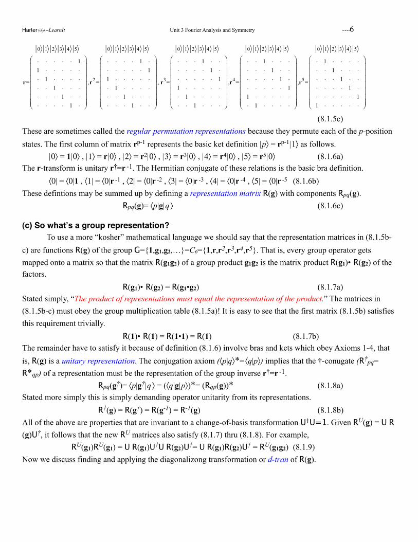
(8.1.5c)These are sometimes called the regular permutation representations because they permute each of the p-position states. The first column of matrix rp-1 represents the basic ket definition |p〉 = rp-1|1〉 as follows. |0〉 = 1|0〉 , |1〉 = r|0〉 , |2〉 = r2|0〉 , |3〉 = r3|0〉 , |4〉 = r4|0〉 , |5〉 = r5|0〉 (8.1.6a)The r-transform is unitary r†=r -1. The Hermitian conjugate of these relations is the basic bra definition. 〈0| = 〈0|1 , 〈1| = 〈0|r -1 , 〈2| = 〈0|r -2 , 〈3| = 〈0|r -3 , 〈4| = 〈0|r -4 , 〈5| = 〈0|r -5 (8.1.6b)These defintions may be summed up by defining a representation matrix R(g) with components Rpq(g). Rpq(g)= 〈p|g|q 〉 (8.1.6c)
(c) So whatʼs a group representation? To use a more “kosher” mathematical language we should say that the representation matrices in (8.1.5b-c) are functions R(g) of the group G={1,g1,g2,…}=C6={1,r,r2,r3,r4,r5}. That is, every group operator gets mapped onto a matrix so that the matrix R(g1g2) of a group product g1g2 is the matrix product R(g1)• R(g2) of the factors. R(g1)• R(g2) = R(g1•g2) (8.1.7a)Stated simply, “The product of representations must equal the representation of the product.” The matrices in (8.1.5b-c) must obey the group multiplication table (8.1.5a)! It is easy to see that the first matrix (8.1.5b) satisfies this requirement trivially. R(1)• R(1) = R(1•1) = R(1) (8.1.7b)The remainder have to satisfy it because of definition (8.1.6) involve bras and kets which obey Axioms 1-4, that is, R(g) is a unitary representation. The conjugation axiom (〈p|q〉*=〈q|p〉) implies that the †-conugate (R†pq= R*qp) of a representation must be the representation of the group inverse r†=r -1. Rpq(g†)= 〈p|g†|q 〉 = (〈q|g|p〉)*= (Rqp(g))* (8.1.8a)Stated more simply this is simply demanding operator unitarity from its representations. R†(g) = R(g†) = R(g-1) = R-1(g) (8.1.8b)All of the above are properties that are invariant to a change-of-basis transformation U†U=1. Given RU(g) = U R(g)U†, it follows that the new RU matrices also satisfy (8.1.7) thru (8.1.8). For example, RU(g1)RU(g1) = U R(g1)U†U R(g2)U†= U R(g1)R(g2)U† = RU(g1g2) (8.1.9)Now we discuss finding and applying the diagonalizong transformation or d-tran of R(g).
HarterSoft –LearnIt Unit 3 Fourier Analysis and Symmetry ----6
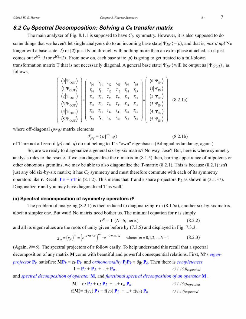
7
8.2 CN Spectral Decomposition: Solving a C6 transfer matrix The main analyzer of Fig. 8.1.1 is supposed to have C6 symmetry. However, it is also supposed to do
some things that we haven't let single analyzers do to an incoming base state |ΨIN 〉 =|p〉, and that is, mix it up! No longer will a base state |1〉 or |2〉 just fly on through with nothing more than an extra phase attached, so it just comes out eiΩ1|1〉 or eiΩ2|2〉 . From now on, each base state |p〉 is going to get treated to a full-blown transformation matrix Τ that is not necessarily diagonal. A general base state |ΨIN 〉 will be output as |ΨOUT〉 , as follows,
0 ΨOUT
1 ΨOUT
2 ΨOUT
3 ΨOUT
4 ΨOUT
5 ΨOUT
⎛
⎝
⎜⎜⎜⎜⎜⎜⎜⎜⎜⎜
⎞
⎠
⎟⎟⎟⎟⎟⎟⎟⎟⎟⎟
=
T00 T01 T02 T03 T04 T05
T10 T11 T12 T13 T14 T15
T20 T21 T22 T23 T24 T25
T30 T31 T32 T33 T34 T35
T40 T41 T42 T43 T44 T45
T50 T51 T52 T53 T54 T55
⎛
⎝
⎜⎜⎜⎜⎜⎜⎜⎜⎜
⎞
⎠
⎟⎟⎟⎟⎟⎟⎟⎟⎟
•
0 ΨIN
1 ΨIN
2 ΨIN
3 ΨIN
4 ΨIN
5 ΨIN
⎛
⎝
⎜⎜⎜⎜⎜⎜⎜⎜⎜⎜
⎞
⎠
⎟⎟⎟⎟⎟⎟⎟⎟⎟⎟
(8.2.1a)
where off-diagonal (p≠q) matrix elements Tpq = 〈 p | Τ | q 〉 (8.2.1b)of T are not all zero if |p〉 and |q〉 do not belong to T‘s "own" eigenbasis. (Bilingual redundancy, again.) So, are we ready to diagonalize a general six-by-six matrix? No way, Jose'! But, here is where symmetry analysis rides to the rescue. If we can diagonalize the r-matrix in (8.1.5) then, barring appearance of nilpotents or other obnoxious gremlins, we may be able to also diagonalize the T-matrix (8.2.1). This is because (8.2.1) isn't just any old six-by-six matrix; it has C6 symmetry and must therefore commute with each of its symmetry operators like r. Recall T r = r T in (8.1.2). This means that T and r share projectors Pk as shown in (3.1.37). Diagonalize r and you may have diagonalized T as well!
(a) Spectral decomposition of symmetry operators rp
The problem of analyzing (8.2.1) is then reduced to diagonalizing r in (8.1.5a), another six-by-six matrix, albeit a simpler one. But wait! No matrix need bother us. The minimal equation for r is simply rN = 1 (N=6, here.) (8.2.2)and all its eigenvalues are the roots of unity given before by (7.3.5) and displayed in Fig. 7.3.3.
χm = rN( )m = e−i 2π / N( )m =e−i 2π m/ N where: m = 0,1,2,..., N −1 (8.2.3)
(Again, N=6). The spectral projectors of r follow easily. To help understand this recall that a spectral decomposition of any matrix M come with beautiful and powerful consequential relations. First, M‘s eigen- projector Pk satisfies: MPk = εk Pk and orthonormality PjPk = δjk Pk. Then there is completeness 1 = P1 + P2 + ...+ Pn . (3.1.15d)repeated and spectral decomposition of operator M, and functional spectral decomposition of an operator M . M = ε1 P1 + ε2 P2 + ...+ εn Pn (3.1.15e)repeated
f(M)= f(ε1) P1 + f(ε2) P2 + ...+ f(εn) Pn (3.1.17)repeated
©2013 W. G. Harter Chapter 8. Fourier Symmetry ! 8--
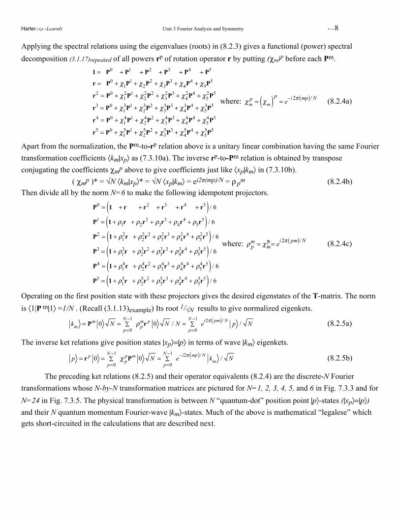
Applying the spectral relations using the eigenvalues (roots) in (8.2.3) gives a functional (power) spectral decomposition (3.1.17)repeated of all powers rp of rotation operator r by putting (χm)p before each Pm.
1 = P0 + P1 + P2 + P3 + P4 + P5
r = P0 + χ1P1 + χ2P2 + χ3P3 + χ4P4 + χ5P5
r2 = P0 + χ12P1 + χ2
2P2 + χ32P3 + χ4
2P4 + χ52P5
r3 = P0 + χ13P1 + χ2
3P2 + χ33P3 + χ4
3P4 + χ53P5
r4 = P0 + χ14P1 + χ2
4P2 + χ34P3 + χ4
4P4 + χ54P5
r5 = P0 + χ15P1 + χ2
5P2 + χ35P3 + χ4
5P4 + χ55P5
where: χm
p = χm( )p= e−i 2π mp( )/ N (8.2.4a)
Apart from the normalization, the Pm-to-rp relation above is a unitary linear combination having the same Fourier transformation coefficients 〈km|xp〉 as (7.3.10a). The inverse rp-to-Pm relation is obtained by transpose conjugating the coefficients χmp above to give coefficients just like 〈xp|km〉 in (7.3.10b). ( χmp )* = √N 〈km|xp〉* = √N 〈xp|km〉 = ei2π(mp)/N = ρ pm (8.2.4b)Then divide all by the norm N=6 to make the following idempotent projectors.
P0 = 1 + r + r2 + r3 + r4 + r5( ) / 6
P1 = 1 + ρ1r + ρ2r2 + ρ3r3 + ρ4r4 + ρ5r5( ) / 6
P2 = 1 + ρ12r + ρ2
2r2 + ρ32r3 + ρ4
2r4 + ρ52r5( ) / 6
P3 = 1 + ρ13r + ρ2
3r2 + ρ33r3 + ρ4
3r4 + ρ53r5( ) / 6
P4 = 1 + ρ14r + ρ2
4r2 + ρ34r3 + ρ4
4r4 + ρ54r5( ) / 6
P5 = 1 + ρ15r + ρ2
5r2 + ρ35r3 + ρ4
5r4 + ρ55r5( ) / 6
where: ρp
m = χmp* = ei 2π pm( )/ N (8.2.4c)
Operating on the first position state with these projectors gives the desired eigenstates of the T-matrix. The norm is 〈1|P m|1〉 =1/N . (Recall (3.1.13)example) Its root 1/√N results to give normalized eigenkets.
km = Pm 0 N =
p=0
N −1∑ ρp
mr p 0 N / N =p=0
N −1∑ ei2π pm( )/ N p / N (8.2.5a)
The inverse ket relations give position states |xp〉=|p〉 in terms of wave |km〉 eigenkets.
p = r p 0 =p=0
N −1∑ χ p
pPm 0 N =p=0
N −1∑ e−i2π mp( )/ N km / N (8.2.5b)
The preceding ket relations (8.2.5) and their operator equivalents (8.2.4) are the discrete-N Fourier transformations whose N-by-N transformation matrices are pictured for N=1, 2, 3, 4, 5, and 6 in Fig. 7.3.3 and for N=24 in Fig. 7.3.5. The physical transformation is between N “quantum-dot” position point |p〉-states (|xp〉=|p〉) and their N quantum momentum Fourier-wave |km〉-states. Much of the above is mathematical “legalese” which gets short-circuited in the calculations that are described next.
HarterSoft –LearnIt Unit 3 Fourier Analysis and Symmetry ----8
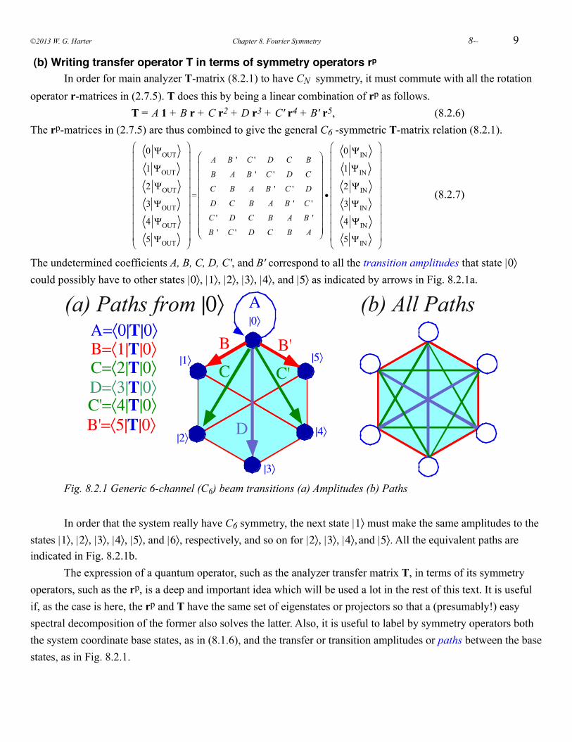
9
(b) Writing transfer operator T in terms of symmetry operators rp In order for main analyzer T-matrix (8.2.1) to have CN symmetry, it must commute with all the rotation operator r-matrices in (2.7.5). T does this by being a linear combination of rp as follows. T = A 1 + B r + C r2 + D r3 + C' r4 + B' r5, (8.2.6) The rp-matrices in (2.7.5) are thus combined to give the general C6 -symmetric T-matrix relation (8.2.1).
0 ΨOUT
1 ΨOUT
2 ΨOUT
3 ΨOUT
4 ΨOUT
5 ΨOUT
⎛
⎝
⎜⎜⎜⎜⎜⎜⎜⎜⎜⎜
⎞
⎠
⎟⎟⎟⎟⎟⎟⎟⎟⎟⎟
=
A B ' C ' D C B
B A B ' C ' D C
C B A B ' C ' D
D C B A B ' C '
C ' D C B A B '
B ' C ' D C B A
⎛
⎝
⎜⎜⎜⎜⎜⎜⎜⎜
⎞
⎠
⎟⎟⎟⎟⎟⎟⎟⎟
•
0 ΨIN
1 ΨIN
2 ΨIN
3 ΨIN
4 ΨIN
5 ΨIN
⎛
⎝
⎜⎜⎜⎜⎜⎜⎜⎜⎜⎜
⎞
⎠
⎟⎟⎟⎟⎟⎟⎟⎟⎟⎟
(8.2.7)
The undetermined coefficients A, B, C, D, C', and B' correspond to all the transition amplitudes that state |0〉 could possibly have to other states |0〉, |1〉, |2〉, |3〉, |4〉, and |5〉 as indicated by arrows in Fig. 8.2.1a.
!
|0〉A
B B'C C'
D
|1〉
|2〉
|3〉
|4〉
|5〉
(a) Paths from |0〉 (b) All Paths
Β=〈1|T|0〉Α=〈0|T|0〉
C=〈2|T|0〉D=〈3|T|0〉C'=〈4|T|0〉B'=〈5|T|0〉
Fig. 8.2.1 Generic 6-channel (C6) beam transitions (a) Amplitudes (b) Paths
In order that the system really have C6 symmetry, the next state |1〉 must make the same amplitudes to the states |1〉, |2〉, |3〉, |4〉, |5〉, and |6〉, respectively, and so on for |2〉, |3〉, |4〉, and |5〉. All the equivalent paths are indicated in Fig. 8.2.1b. The expression of a quantum operator, such as the analyzer transfer matrix T, in terms of its symmetry operators, such as the rp, is a deep and important idea which will be used a lot in the rest of this text. It is useful if, as the case is here, the rp and T have the same set of eigenstates or projectors so that a (presumably!) easy spectral decomposition of the former also solves the latter. Also, it is useful to label by symmetry operators both the system coordinate base states, as in (8.1.6), and the transfer or transition amplitudes or paths between the base states, as in Fig. 8.2.1.
©2013 W. G. Harter Chapter 8. Fourier Symmetry ! 8--
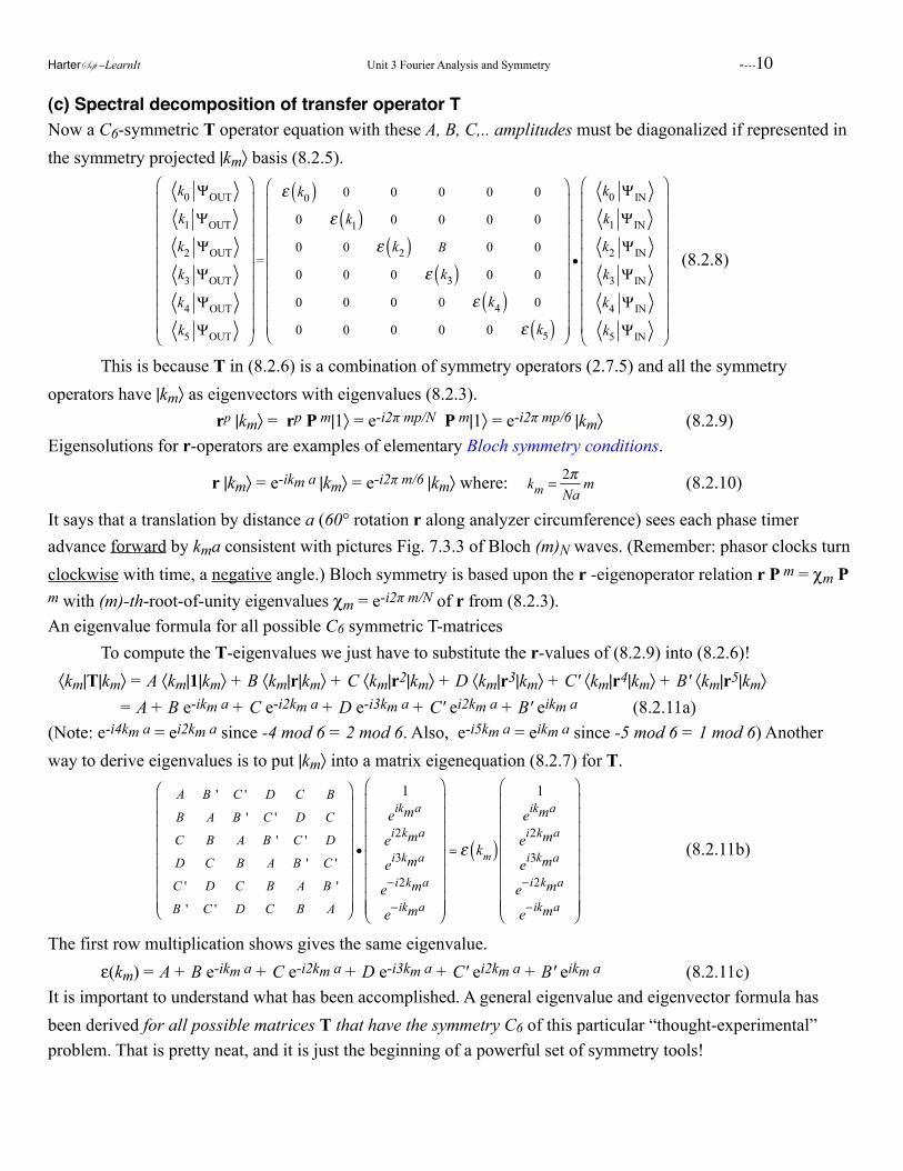
(c) Spectral decomposition of transfer operator T Now a C6-symmetric T operator equation with these A, B, C,.. amplitudes must be diagonalized if represented in the symmetry projected |km〉 basis (8.2.5).
k0 ΨOUT
k1 ΨOUT
k2 ΨOUT
k3 ΨOUT
k4 ΨOUT
k5 ΨOUT
⎛
⎝
⎜⎜⎜⎜⎜⎜⎜⎜⎜⎜
⎞
⎠
⎟⎟⎟⎟⎟⎟⎟⎟⎟⎟
=
ε k0( ) 0 0 0 0 0
0 ε k1( ) 0 0 0 0
0 0 ε k2( ) B 0 0
0 0 0 ε k3( ) 0 0
0 0 0 0 ε k4( ) 0
0 0 0 0 0 ε k5( )
⎛
⎝
⎜⎜⎜⎜⎜⎜⎜⎜⎜⎜
⎞
⎠
⎟⎟⎟⎟⎟⎟⎟⎟⎟⎟
•
k0 ΨIN
k1 ΨIN
k2 ΨIN
k3 ΨIN
k4 ΨIN
k5 ΨIN
⎛
⎝
⎜⎜⎜⎜⎜⎜⎜⎜⎜⎜
⎞
⎠
⎟⎟⎟⎟⎟⎟⎟⎟⎟⎟
(8.2.8)
This is because T in (8.2.6) is a combination of symmetry operators (2.7.5) and all the symmetry operators have |km〉 as eigenvectors with eigenvalues (8.2.3). rp |km〉 = rp P m|1〉 = e-i2π mp/N P m|1〉 = e-i2π mp/6 |km〉 (8.2.9)Eigensolutions for r-operators are examples of elementary Bloch symmetry conditions.
r |km〉 = e-ikm a |km〉 = e-i2π m/6 |km〉 where: km = 2π
Nam (8.2.10)
It says that a translation by distance a (60° rotation r along analyzer circumference) sees each phase timer advance forward by kma consistent with pictures Fig. 7.3.3 of Bloch (m)N waves. (Remember: phasor clocks turn clockwise with time, a negative angle.) Bloch symmetry is based upon the r -eigenoperator relation r P m = χm P m with (m)-th-root-of-unity eigenvalues χm = e-i2π m/N of r from (8.2.3). An eigenvalue formula for all possible C6 symmetric T-matrices To compute the T-eigenvalues we just have to substitute the r-values of (8.2.9) into (8.2.6)! 〈km|T|km〉 = A 〈km|1|km〉 + B 〈km|r|km〉 + C 〈km|r2|km〉 + D 〈km|r3|km〉 + C' 〈km|r4|km〉 + B' 〈km|r5|km〉6 = A + B e-ikm a + C e-i2km a + D e-i3km a + C' ei2km a + B' eikm a (8.2.11a) (Note: e-i4km a = ei2km a since -4 mod 6 = 2 mod 6. Also, e-i5km a = eikm a since -5 mod 6 = 1 mod 6) Another way to derive eigenvalues is to put |km〉 into a matrix eigenequation (8.2.7) for T.
A B ' C ' D C B
B A B ' C ' D C
C B A B ' C ' D
D C B A B ' C '
C ' D C B A B '
B ' C ' D C B A
⎛
⎝
⎜⎜⎜⎜⎜⎜⎜⎜
⎞
⎠
⎟⎟⎟⎟⎟⎟⎟⎟
•
1
eikma
ei2kma
ei3kma
e−i2kma
e−ikma
⎛
⎝
⎜⎜⎜⎜⎜⎜⎜⎜⎜
⎞
⎠
⎟⎟⎟⎟⎟⎟⎟⎟⎟
= ε km( )
1
eikma
ei2kma
ei3kma
e−i2kma
e−ikma
⎛
⎝
⎜⎜⎜⎜⎜⎜⎜⎜⎜
⎞
⎠
⎟⎟⎟⎟⎟⎟⎟⎟⎟
(8.2.11b)
The first row multiplication shows gives the same eigenvalue. ε(km) = A + B e-ikm a + C e-i2km a + D e-i3km a + C' ei2km a + B' eikm a (8.2.11c) It is important to understand what has been accomplished. A general eigenvalue and eigenvector formula has been derived for all possible matrices T that have the symmetry C6 of this particular “thought-experimental” problem. That is pretty neat, and it is just the beginning of a powerful set of symmetry tools!
HarterSoft –LearnIt Unit 3 Fourier Analysis and Symmetry ----10
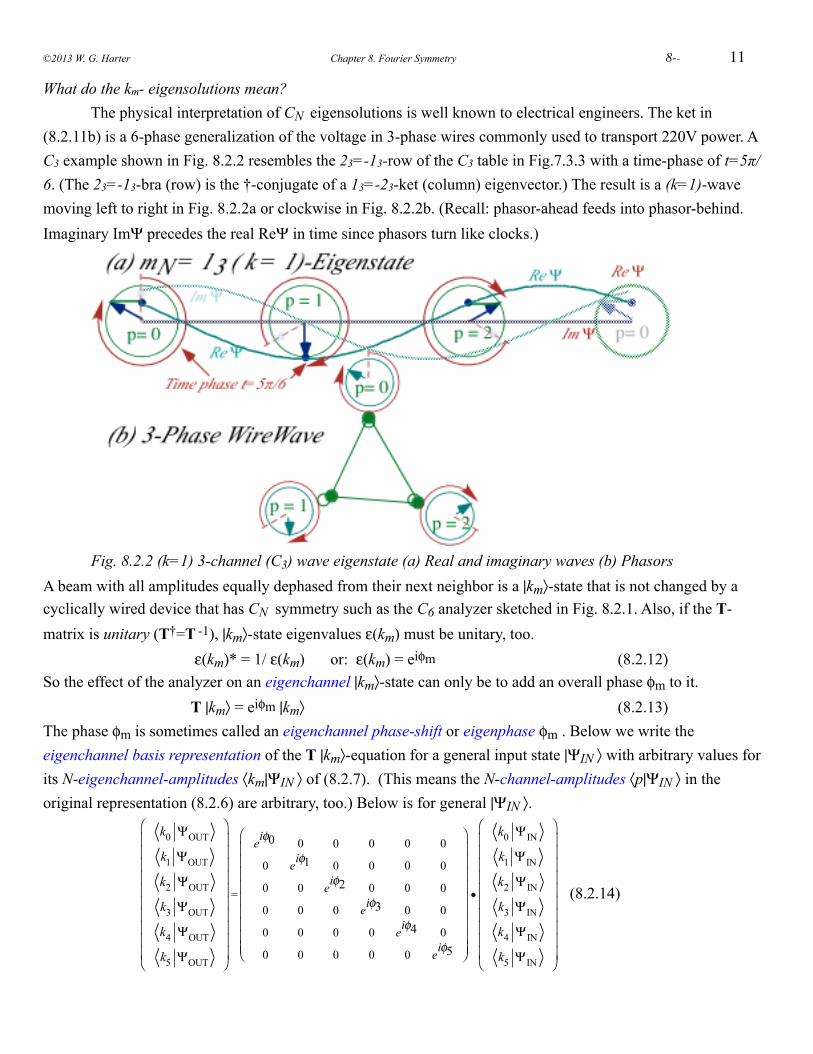
11
What do the km- eigensolutions mean? The physical interpretation of CN eigensolutions is well known to electrical engineers. The ket in (8.2.11b) is a 6-phase generalization of the voltage in 3-phase wires commonly used to transport 220V power. A C3 example shown in Fig. 8.2.2 resembles the 23=-13-row of the C3 table in Fig.7.3.3 with a time-phase of t=5π/6. (The 23=-13-bra (row) is the †-conjugate of a 13=-23-ket (column) eigenvector.) The result is a (k=1)-wave moving left to right in Fig. 8.2.2a or clockwise in Fig. 8.2.2b. (Recall: phasor-ahead feeds into phasor-behind. Imaginary ImΨ precedes the real ReΨ in time since phasors turn like clocks.)
Fig. 8.2.2 (k=1) 3-channel (C3) wave eigenstate (a) Real and imaginary waves (b) PhasorsA beam with all amplitudes equally dephased from their next neighbor is a |km〉-state that is not changed by a cyclically wired device that has CN symmetry such as the C6 analyzer sketched in Fig. 8.2.1. Also, if the T-matrix is unitary (T†=T -1), |km〉-state eigenvalues ε(km) must be unitary, too. ε(km)* = 1/ ε(km) or: ε(km) = eiφm (8.2.12)So the effect of the analyzer on an eigenchannel |km〉-state can only be to add an overall phase φm to it. T |km〉 = eiφm |km〉 (8.2.13)The phase φm is sometimes called an eigenchannel phase-shift or eigenphase φm . Below we write the eigenchannel basis representation of the T |km〉-equation for a general input state |ΨIN 〉 with arbitrary values for its N-eigenchannel-amplitudes 〈km|ΨIN 〉 of (8.2.7). (This means the N-channel-amplitudes 〈p|ΨIN 〉 in the original representation (8.2.6) are arbitrary, too.) Below is for general |ΨIN 〉.
k0 ΨOUT
k1 ΨOUT
k2 ΨOUT
k3 ΨOUT
k4 ΨOUT
k5 ΨOUT
⎛
⎝
⎜⎜⎜⎜⎜⎜⎜⎜⎜⎜
⎞
⎠
⎟⎟⎟⎟⎟⎟⎟⎟⎟⎟
=
eiφ0 0 0 0 0 0
0 eiφ1 0 0 0 0
0 0 eiφ2 0 0 0
0 0 0 eiφ3 0 0
0 0 0 0 eiφ4 0
0 0 0 0 0 eiφ5
⎛
⎝
⎜⎜⎜⎜⎜⎜⎜⎜⎜
⎞
⎠
⎟⎟⎟⎟⎟⎟⎟⎟⎟
•
k0 ΨIN
k1 ΨIN
k2 ΨIN
k3 ΨIN
k4 ΨIN
k5 ΨIN
⎛
⎝
⎜⎜⎜⎜⎜⎜⎜⎜⎜⎜
⎞
⎠
⎟⎟⎟⎟⎟⎟⎟⎟⎟⎟
(8.2.14)
©2013 W. G. Harter Chapter 8. Fourier Symmetry ! 8--
(d) OK, where did those eikx wavefunctions come from? Every student of differential equations is told early on to try the exponential solutions eAt or eiat in independent variable t with little reason given except, "It works!...sometimes." Now we can see why and when
such solutions work. The key to our exponential eigenfunctions ψkm(xp)= eikmxp /√N was CN symmetry which demanded in (2.7.5) that we use roots of unity, that is, the roots of the minimal equation rN=1 for symmetry operator r. If we let N approach infinity (N→∞) the symmetry approaches continuous translation symmetry C∞, and the eigenfunctions ψkm(xp) approach plane waves ψk(x)= eikx /√2π such as given by (2.6.20b) in Sec. 2.6b. Symmetry demands independence or invariance to translation of the independent variable x. In other words, you should get the same differential equation no matter whether you let the origin be at x=0 or at x=2,517 in Timbuktu. For example, the differential equation
d2ψdx2
+ 2γ dψdx
+ k2ψ = 0 (8.2.15)
does have C∞ symmetry so eikx will work, but an equation like
d2ψdx2
+ 2γ xdψdx
+ k2x2ψ = 0 (8.2.16)
does not have C∞ symmetry because of the x-dependence; it's not the same equation in Timbuktu. An example of a CN -symmetric differential equation is Matieu's equation for waves in a periodic solid.
d2ψdx2
+ k2 cos(Nx)ψ = 0
All that we have said applies as well when the independent variable is time t. For example, the differential equation
d2ψdt2
+ 2Γ dψdt
+ω 2ψ = 0
does have C∞ symmetry so eiωt will work. An example of a CN -symmetric time differential equation is Mathieu's equation for a periodic force. Later we use CN -symmetry to help solve this type of equation.
d2ψdt2
+ k2 cos(Nt)ψ = 0
HarterSoft –LearnIt Unit 3 Fourier Analysis and Symmetry ----12
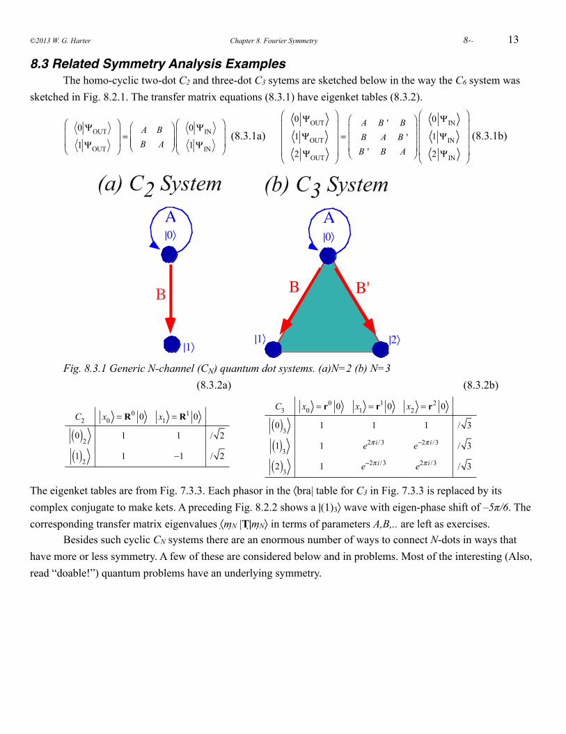
13
8.3 Related Symmetry Analysis Examples The homo-cyclic two-dot C2 and three-dot C3 sytems are sketched below in the way the C6 system was sketched in Fig. 8.2.1. The transfer matrix equations (8.3.1) have eigenket tables (8.3.2).
0 ΨOUT
1 ΨOUT
⎛
⎝
⎜⎜
⎞
⎠
⎟⎟=
A BB A
⎛
⎝⎜⎜
⎞
⎠⎟⎟
0 ΨIN
1 ΨIN
⎛
⎝
⎜⎜
⎞
⎠
⎟⎟
(8.3.1a)
0 ΨOUT
1 ΨOUT
2 ΨOUT
⎛
⎝
⎜⎜⎜⎜
⎞
⎠
⎟⎟⎟⎟
=A B ' BB A B 'B ' B A
⎛
⎝
⎜⎜⎜
⎞
⎠
⎟⎟⎟
0 ΨIN
1 ΨIN
2 ΨIN
⎛
⎝
⎜⎜⎜⎜
⎞
⎠
⎟⎟⎟⎟
(8.3.1b)
(a) C2 System
|0〉A
|1〉
(b) C3 System
|0〉A
|1〉 |2〉
B B'B
Fig. 8.3.1 Generic N-channel (CN) quantum dot systems. (a)N=2 (b) N=3 (8.3.2a) (8.3.2b)
C2 x0 = R0 0 x1 = R1 0
0( )2 1 1 / 2
1( )2 1 −1 / 2
C3 x0 = r0 0 x1 = r1 0 x2 = r2 0
0( )3 1 1 1 / 3
1( )3 1 e2π i /3 e−2π i /3 / 3
2( )3 1 e−2π i /3 e2π i /3 / 3
The eigenket tables are from Fig. 7.3.3. Each phasor in the 〈bra| table for C3 in Fig. 7.3.3 is replaced by its complex conjugate to make kets. A preceding Fig. 8.2.2 shows a |(1)3〉 wave with eigen-phase shift of –5π/6. The corresponding transfer matrix eigenvalues 〈 m N |T| m N〉 in terms of parameters A,B,.. are left as exercises. Besides such cyclic CN systems there are an enormous number of ways to connect N-dots in ways that have more or less symmetry. A few of these are considered below and in problems. Most of the interesting (Also, read “doable!”) quantum problems have an underlying symmetry.
©2013 W. G. Harter Chapter 8. Fourier Symmetry ! 8--
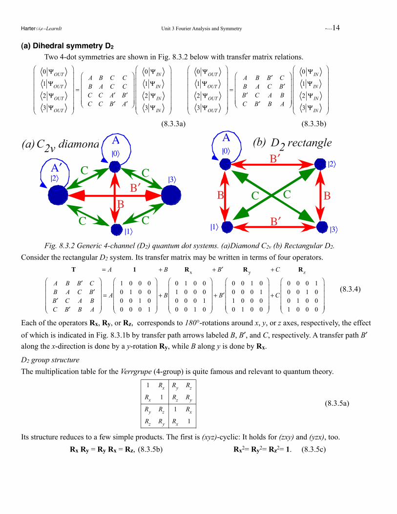
(a) Dihedral symmetry D2
Two 4-dot symmetries are shown in Fig. 8.3.2 below with transfer matrix relations.
0 ΨOUT
1 ΨOUT
2 ΨOUT
3 ΨOUT
⎛
⎝
⎜⎜⎜⎜⎜⎜
⎞
⎠
⎟⎟⎟⎟⎟⎟
=
A B C CB A C CC C ′A ′BC C ′B ′A
⎛
⎝
⎜⎜⎜⎜
⎞
⎠
⎟⎟⎟⎟
0 Ψ IN
1 Ψ IN
2 Ψ IN
3 Ψ IN
⎛
⎝
⎜⎜⎜⎜⎜⎜
⎞
⎠
⎟⎟⎟⎟⎟⎟
0 ΨOUT
1 ΨOUT
2 ΨOUT
3 ΨOUT
⎛
⎝
⎜⎜⎜⎜⎜⎜
⎞
⎠
⎟⎟⎟⎟⎟⎟
=
A B ′B CB A C ′B′B C A B
C ′B B A
⎛
⎝
⎜⎜⎜⎜
⎞
⎠
⎟⎟⎟⎟
0 Ψ IN
1 Ψ IN
2 Ψ IN
3 Ψ IN
⎛
⎝
⎜⎜⎜⎜⎜⎜
⎞
⎠
⎟⎟⎟⎟⎟⎟
(8.3.3a) (8.3.3b)
(a)|0〉A
|1〉
B
|2〉A′
B′C
|3〉
|0〉A
|1〉
B
|2〉
|3〉
BC
B′
B′
(b)C2v diamond D2 rectangle
C
C
C
C
Fig. 8.3.2 Generic 4-channel (D2) quantum dot systems. (a)Diamond C2v (b) Rectangular D2.Consider the rectangular D2 system. Its transfer matrix may be written in terms of four operators.
T = A 1 + B Rx + ′B Ry +C Rz
A B ′B CB A C ′B′B C A B
C ′B B A
⎛
⎝
⎜⎜⎜⎜
⎞
⎠
⎟⎟⎟⎟
= A
1 0 0 00 1 0 00 0 1 00 0 0 1
⎛
⎝
⎜⎜⎜⎜
⎞
⎠
⎟⎟⎟⎟
+ B
0 1 0 01 0 0 00 0 0 10 0 1 0
⎛
⎝
⎜⎜⎜⎜
⎞
⎠
⎟⎟⎟⎟
+ ′B
0 0 1 00 0 0 11 0 0 00 1 0 0
⎛
⎝
⎜⎜⎜⎜
⎞
⎠
⎟⎟⎟⎟
+C
0 0 0 10 0 1 00 1 0 01 0 0 0
⎛
⎝
⎜⎜⎜⎜
⎞
⎠
⎟⎟⎟⎟
(8.3.4)
Each of the operators Rx, Ry, or Rz, corresponds to 180°-rotations around x, y, or z axes, respectively, the effect of which is indicated in Fig. 8.3.1b by transfer path arrows labeled B, B′, and C, respectively. A transfer path B′ along the x-direction is done by a y-rotation Ry, while B along y is done by Rx.
D2 group structureThe multiplication table for the Verrgrupe (4-group) is quite famous and relevant to quantum theory.
1 Rx Ry Rz
Rx 1 Rz Ry
Ry Rz 1 Rx
Rz Ry Rx 1
(8.3.5a)
Its structure reduces to a few simple products. The first is (xyz)-cyclic: It holds for (zxy) and (yzx), too. Rx Ry = Ry Rx = Rz, (8.3.5b) Rx2= Ry2= Rz2= 1. (8.3.5c)
HarterSoft –LearnIt Unit 3 Fourier Analysis and Symmetry ----14
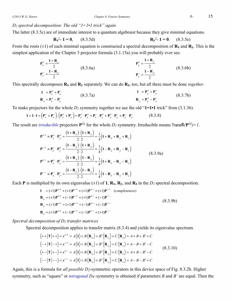
15
D2 spectral decomposition: The old “1=1•1 trick” againThe latter (8.3.5c) are of immediate interest to a quantum algebraist because they give minimal equations. Rx2- 1 = 0, (8.3.5d) Ry2- 1 = 0. (8.3.5e)From the roots (±1) of each minimal equation is constructed a spectral decomposition of Rx and Ry. This is the simplest application of the Chapter 3 projector formula (3.1.15a) you will probably ever see.
Px+ =
1 + Rx2
Px− =
1 − Rx2
(8.3.6a)
Py+ =
1 + R y
2
Py− =
1 − R y
2
(8.3.6b)
This spectrally decomposes Rx and Ry separately. We can do Rz, too, but all three must be done together.
1 = Px+ + Px
−
Rx = Px+ − Px
− (8.3.7a)
1 = Py+ + Py
−
R y = Py+ − Py
− (8.3.7b)
To make projectors for the whole D2 symmetry together we use the old “1=1•1 trick” from (3.1.36).
1 = 1 ⋅1 = Px
+ + Px−( ) ⋅ Py
+ + Py−( ) = Px
+ ⋅Py+ + Px
− ⋅Py+ + Px
+ ⋅Py− + Px
− ⋅Py− (8.3.8)
The result are irreducible projectors P(i) for the whole D2 symmetry. Irreducible means TraceR(P(i))=1.
P++ ≡ Px+ ⋅Py
+ =1 + Rx( ) ⋅ 1 + R y( )
2 ⋅2= 1
41 + Rx + R y + R z( )
P−+ ≡ Px− ⋅Py
+ =1 − Rx( ) ⋅ 1 + R y( )
2 ⋅2= 1
41 − Rx + R y − R z( )
P+− ≡ Px+ ⋅Py
− =1 + Rx( ) ⋅ 1 − R y( )
2 ⋅2= 1
41 + Rx − R y − R z( )
P−− ≡ Px− ⋅Py
− =1 − Rx( ) ⋅ 1 − R y( )
2 ⋅2= 1
41 − Rx − R y + R z( )
(8.3.9a)
Each P is multiplied by its own eigenvalue (±1) of 1, Rx, Ry, and Rz in the D2 spectral decomposition.
1 = (+1)P++ + (+1)P−+ + (+1)P+− + (+1)P−− (completeness)
Rx = (+1)P++ + (−1)P−+ + (+1)P+− + (−1)P−−
R y = (+1)P++ + (+1)P−+ + (−1)P+− + (−1)P−−
R z = (+1)P++ + (−1)P−+ + (−1)P+− + (+1)P−−
(8.3.9b)
Spectral decomposition of D2 transfer matrices Spectral decomposition applies to transfer matrix (8.3.4) and yields its eigenvalue spectrum.
+ + T + + = ε++ = A 1 + B Rx + ′B R y + C R z = A+ B + ′B + C
− + T − + = ε−+ = A 1 + B Rx + ′B R y + C R z = A− B + ′B − C
+ − T + − = ε+− = A 1 + B Rx + ′B R y + C R z = A+ B − ′B − C
− − T − − = ε−− = A 1 + B Rx + ′B R y + C R z = A− B − ′B + C
(8.3.10)
Again, this is a formula for all possible D2-symmetric operators in this device space of Fig. 8.3.2b. Higher symmetry, such as “square” or tetragonal D4–symmetry is obtained if parameters B and B’ are equal. Then the
©2013 W. G. Harter Chapter 8. Fourier Symmetry ! 8--
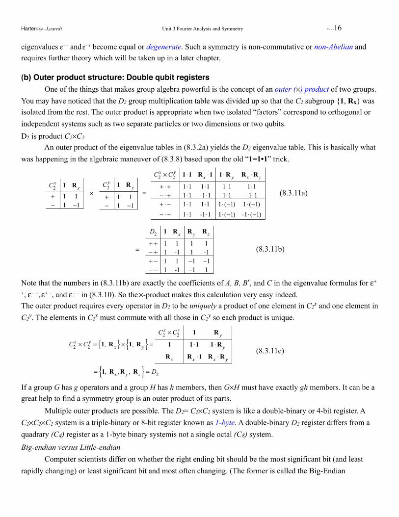
eigenvalues ε+ − and ε− + become equal or degenerate. Such a symmetry is non-commutative or non-Abelian and requires further theory which will be taken up in a later chapter.
(b) Outer product structure: Double qubit registers One of the things that makes group algebra powerful is the concept of an outer (×) product of two groups. You may have noticed that the D2 group multiplication table was divided up so that the C2 subgroup {1, Rx} was isolated from the rest. The outer product is appropriate when two isolated “factors” correspond to orthogonal or independent systems such as two separate particles or two dimensions or two qubits. D2 is product C2×C2 An outer product of the eigenvalue tables in (8.3.2a) yields the D2 eigenvalue table. This is basically what was happening in the algebraic maneuver of (8.3.8) based upon the old “1=1•1” trick.
C2x 1 Rx
+ 1 1− 1 −1
× C2
y 1 R y
+ 1 1− 1 −1
=
C2x × C2
y 1 ⋅1 Rx ⋅1 1 ⋅R y Rx ⋅R y
+ ⋅+ 1⋅1 1⋅1 1⋅1 1⋅1− ⋅+ 1⋅1 -1⋅1 1⋅1 -1⋅1+ ⋅ − 1⋅1 1⋅1 1⋅ (−1) 1⋅ (−1)− ⋅ − 1⋅1 -1⋅1 1⋅ (−1) -1⋅ (−1)
(8.3.11a)
=
D2 1 Rx R y R z
+ + 1 1 1 1− + 1 -1 1 -1+ − 1 1 −1 −1− − 1 -1 −1 1
(8.3.11b)
Note that the numbers in (8.3.11b) are exactly the coefficients of A, B, B′, and C in the eigenvalue formulas for ε+
+, ε− +, ε+ −, and ε− − in (8.3.10). So the ×-product makes this calculation very easy indeed.The outer product requires every operator in D2 to be uniquely a product of one element in C2x and one element in C2y. The elements in C2x must commute with all those in C2y so each product is unique.
C2x × C2
y = 1, Rx{ } × 1, R y{ } =C2
x × C2y 1 R y
1 1 ⋅1 1 ⋅R y
Rx Rx ⋅1 Rx ⋅R y
= 1, Rx ,R y , R z{ } = D2
(8.3.11c)
If a group G has g operators and a group H has h members, then G×H must have exactly gh members. It can be a great help to find a symmetry group is an outer product of its parts. Multiple outer products are possible. The D2= C2×C2 system is like a double-binary or 4-bit register. A C2×C2×C2 system is a triple-binary or 8-bit register known as 1-byte. A double-binary D2 register differs from a quadrary (C4) register as a 1-byte binary systemis not a single octal (C8) system.
Big-endian versus Little-endian Computer scientists differ on whether the right ending bit should be the most significant bit (and least rapidly changing) or least significant bit and most often changing. (The former is called the Big-Endian
HarterSoft –LearnIt Unit 3 Fourier Analysis and Symmetry ----16
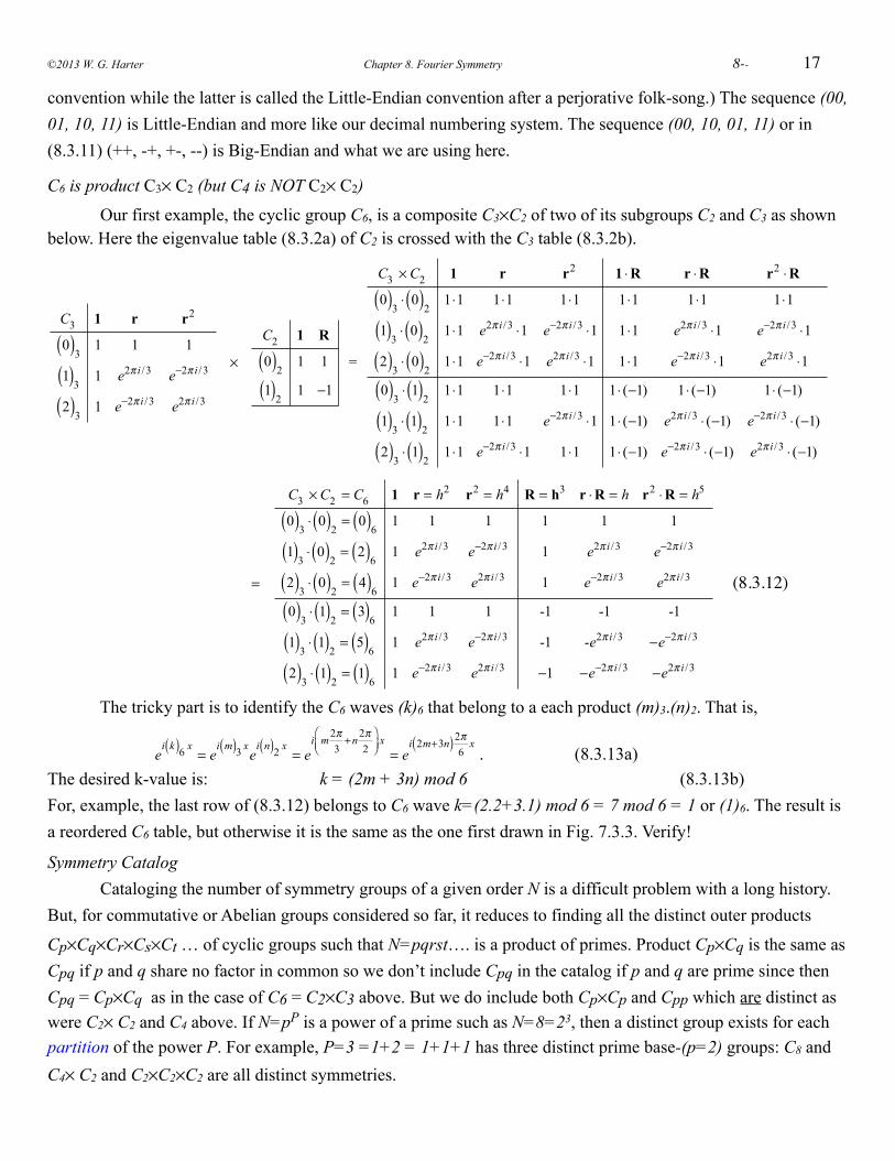
17
convention while the latter is called the Little-Endian convention after a perjorative folk-song.) The sequence (00, 01, 10, 11) is Little-Endian and more like our decimal numbering system. The sequence (00, 10, 01, 11) or in (8.3.11) (++, -+, +-, --) is Big-Endian and what we are using here.
C6 is product C3× C2 (but C4 is NOT C2× C2)
Our first example, the cyclic group C6, is a composite C3×C2 of two of its subgroups C2 and C3 as shown below. Here the eigenvalue table (8.3.2a) of C2 is crossed with the C3 table (8.3.2b).
C3 1 r r2
0( )3 1 1 1
1( )3 1 e2π i /3 e−2π i /3
2( )3 1 e−2π i /3 e2π i /3
×
C2 1 R
0( )2 1 1
1( )2 1 −1
=
C3 × C2 1 r r2 1 ⋅R r ⋅R r2 ⋅R
0( )3 ⋅ 0( )2 1⋅1 1⋅1 1⋅1 1⋅1 1⋅1 1⋅1
1( )3 ⋅ 0( )2 1⋅1 e2π i /3 ⋅1 e−2π i /3 ⋅1 1⋅1 e2π i /3 ⋅1 e−2π i /3 ⋅1
2( )3 ⋅ 0( )2 1⋅1 e−2π i /3 ⋅1 e2π i /3 ⋅1 1⋅1 e−2π i /3 ⋅1 e2π i /3 ⋅1
0( )3 ⋅ 1( )2 1⋅1 1⋅1 1⋅1 1⋅ (−1) 1⋅ (−1) 1⋅ (−1)
1( )3 ⋅ 1( )2 1⋅1 1⋅1 e−2π i /3 ⋅1 1⋅ (−1) e2π i /3 ⋅ (−1) e−2π i /3 ⋅ (−1)
2( )3 ⋅ 1( )2 1⋅1 e−2π i /3 ⋅1 1⋅1 1⋅ (−1) e−2π i /3 ⋅ (−1) e2π i /3 ⋅ (−1)
=
C3 × C2 = C6 1 r = h2 r2 = h4 R = h3 r ⋅R = h r2 ⋅R = h5
0( )3 ⋅ 0( )2 = 0( )6 1 1 1 1 1 1
1( )3 ⋅ 0( )2 = 2( )6 1 e2π i /3 e−2π i /3 1 e2π i /3 e−2π i /3
2( )3 ⋅ 0( )2 = 4( )6 1 e−2π i /3 e2π i /3 1 e−2π i /3 e2π i /3
0( )3 ⋅ 1( )2 = 3( )6 1 1 1 -1 -1 -1
1( )3 ⋅ 1( )2 = 5( )6 1 e2π i /3 e−2π i /3 -1 -e2π i /3 −e−2π i /3
2( )3 ⋅ 1( )2 = 1( )6 1 e−2π i /3 e2π i /3 −1 −e−2π i /3 −e2π i /3
! (8.3.12)
The tricky part is to identify the C6 waves (k)6 that belong to a each product (m)3.(n)2. That is,
ei k( )6 x
= ei m( )3 x
ei n( )2 x
= ei m
2π3+n
2π2
⎛⎝⎜
⎞⎠⎟
x= e
i 2m+3n( )2π6
x. (8.3.13a)
The desired k-value is: k = (2m + 3n) mod 6 (8.3.13b)For, example, the last row of (8.3.12) belongs to C6 wave k=(2.2+3.1) mod 6 = 7 mod 6 = 1 or (1)6. The result is a reordered C6 table, but otherwise it is the same as the one first drawn in Fig. 7.3.3. Verify!
Symmetry Catalog Cataloging the number of symmetry groups of a given order N is a difficult problem with a long history. But, for commutative or Abelian groups considered so far, it reduces to finding all the distinct outer products
Cp×Cq×Cr×Cs×Ct … of cyclic groups such that N=pqrst…. is a product of primes. Product Cp×Cq is the same as Cpq if p and q share no factor in common so we don’t include Cpq in the catalog if p and q are prime since then Cpq = Cp×Cq as in the case of C6 = C2×C3 above. But we do include both Cp×Cp and Cpp which are distinct as were C2× C2 and C4 above. If N=pP is a power of a prime such as N=8=23, then a distinct group exists for each partition of the power P. For example, P=3 =1+2 = 1+1+1 has three distinct prime base-(p=2) groups: C8 and C4× C2 and C2×C2×C2 are all distinct symmetries.
©2013 W. G. Harter Chapter 8. Fourier Symmetry ! 8--
Problems for Chapter 8.Subgroup soup8.1.1 (a) The C6 symmetry group has subgroups. List all of them except C6 itself.(b) Do the same for the symmetry groups C3 , C4 , and C5 . What is special about groups CN of prime order N?
Ttrace’o g8.1.2 (a) By group axioms (Sec. 2.2) show each row and column of a group table has an operator g only once.(b) Use (a) to show that the regular representation trace TraceR(g) is zero for all but “do-nothing” unit operator g=1.Turn-about’s fair play8.2.1 Suppose we are given the eigenvalues {τ0, τ1, τ2, τ3, τ4, τ5} of a unitary C6 transfer matrix T in (8.2.1).(a) Can the {τ0, τ1, τ2, τ3, τ4, τ5} be any old complex numbers? What restrictions, if any, apply?(b) Can one give a formula for all 36 components Tpq of T in terms of {τ0, τ1, τ2, τ3, τ4, τ5}? If so do it. If not expalin why
not and under what conditions you may be able to do it.
A Hex on pairing8.2.2 Suppose the C6 transfer matrix T is the form of the Pairing operator, that is all components equal Tpq = T . (a) Derive the resulting eigenvalue spectrum.(b) What, if any, limitations need to be placed on parameter T? (c) Discuss which waves belong to which eigenvalues
Phase o’Hex8.2.3 (a) Could the hexagonal C6 analyzer be wired so input |even sites〉=(1,0,1,0,1,0) comes out eiφ |even〉? What km-eigenstates make up |even sites 〉? Does your “rewiring” maintain C6 symmetry?(b) Could the C6 analyzer be wired so input |even sites 〉 comes out eiφ |odd sites 〉=(0,1,0,1,0,1)? What km-eigenstates make up |odd sites 〉? Does your “rewiring” maintain C6 symmetry?(c) Could the C6 analyzer be wired so input |odd symm〉=(1,-1,1,-1,1,-1) comes out eiφ |odd symm 〉? What km-eigenstates make up |odd symm 〉? Does your “rewiring” maintain C6 symmetry? (d) Could the C6 analyzer be wired so input | odd symm 〉 comes out eiφ |even symm 〉=(1,1,1,1,1,1)? What km-eigenstates make up | even symm 〉? Does your “rewiring” maintain C6 symmetry?
Little diamond8.3.1. The symmetry eigensolution analysis of the C2v diamond quantum dot device in Fig. 8.3.2(a) is a little different than its D2 cousin in Fig. 8.3.2(b). Symmerty multiplication table and spectral decomposition is essentially the same but the transfer T-operator is not such a simple linear combination of symmetry operators. Represent the symmetry and give a decomposition of symmetry and T-matrix. (Note that x and y-plane mirror reflections are symmetry operators, too. There was no distinction between rotations and reflections in the D2 problem.)
Double Crossed8.3.2. Complete a symmetry catalog of commutative (Abelian) groups in terms of distinct Cp×Cq×... cross products.(a) for order N=8. (b) N=9. (c) N=10. (d) N=11. (e) N=12. (f) N=16.
HarterSoft –LearnIt Unit 3 Fourier Analysis and Symmetry ----18
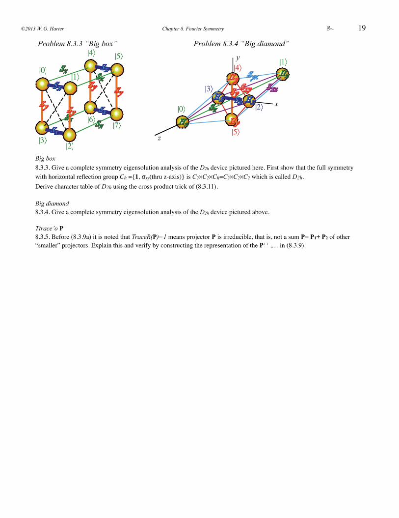
19
|4〉 |5〉
|6〉|7〉
|0〉|1〉
|3〉|2〉
x
y
z
|0〉
|1〉
|2〉
|3〉
|4〉
|5〉
Problem 8.3.3 “Big box” Problem 8.3.4 “Big diamond”
Big box8.3.3. Give a complete symmetry eigensolution analysis of the D2h device pictured here. First show that the full symmetry with horizontal reflection group Ch ={1, σxy(thru z-axis)} is C2×C2×Ch=C2×C2×C2 which is called D2h.Derive character table of D2h using the cross product trick of (8.3.11).
Big diamond8.3.4. Give a complete symmetry eigensolution analysis of the D2h device pictured above.
Ttrace’o P8.3.5. Before (8.3.9a) it is noted that TraceR(P)=1 means projector P is irreducible, that is, not a sum P= P1+ P2 of other “smaller” projectors. Explain this and verify by constructing the representation of the P++ ,… in (8.3.9).
©2013 W. G. Harter Chapter 8. Fourier Symmetry ! 8--
QMfor
AMOPΨChapter 9
Time Evolution and
Fourier Dynamics
W. G. Harter
Now we consider the transfer operator from Hell, the time evolution operator U. This “grim-reaper” of the quantum world determines everything that happens in a non-relativistic (Schrodinger) system. Nothing escapes U-action including you! So learn U well, and pay
particular attention to Uʼs generator H which is called the Hamiltonian. The expression e-iHt (for
constant H) is an icon of modern quantum theory. Quantum dot systems from Chapters 7 and 8 will be used as examples and provide our first introduction to quantum periodic band theory and quantum “revival” beats. (Yes, some waves can survive the grim reaper by reviving repeatedly while doing arithmetic, too!)
HarterSoft –LearnIt Unit 3 Fourier Analysis and Symmetry ----1
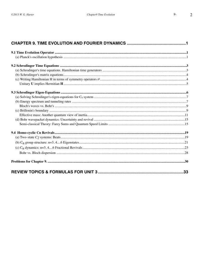
2
...................................................CHAPTER 9. TIME EVOLUTION AND FOURIER DYNAMICS! 1
........................................................................................................................................................9.1 Time Evolution Operator! 1..............................................................................................................................................(a) Planck's oscillation hypothesis! 1
..................................................................................................................................................9.2 Schrodinger Time Equations! 3.................................................................................................(a) Schrodinger's time equations. Hamiltonian time generators! 3
..............................................................................................................................................(b) Schrodinger's matrix equations! 4(c) Writing Hamiltonian H in terms of symmetry operators rp....................................................................................................! 4
Unitary U implies Hermitian H..............................................................................................................................................! 5
.................................................................................................................................................9.3 Schrodinger Eigen-Equations! 6(a) Solving Schrodinger's eigen-equations for C6 ........................................................................................................... system! 7
....................................................................................................................................(b) Energy spectrum and tunneling rates! 7........................................................................................................................................................Bloch's waves vs. Bohr's! 9
(c) Brillouin's .............................................................................................................................................................. boundary! 9.................................................................................................................Effective mass: Another quantum view of inertia! 11
.........................................................................................................(d) Bohr wavepacket dynamics: Uncertainty and revival! 15........................................................................................Semi-classical Theory: Farey Sums and Quantum Speed Limits! 15
......................................................................................................................................................9.4 Homo-cyclic Cn Revivals! 19(a) Two–state C2 ............................................................................................................................................... systems: Beats! 19(b) Cn .......................................................................................................................... group structure: n=3, 4,...6 Eigenstates! 21(c) Cn ...................................................................................................................... dynamics: n=3, 4,...6 Fractional Revivals! 23
....................................................................................................................................................Bohr vs. Bloch dispersion! 28
..............................................................................................................................................................Problems for Chapter 9.! 30
..........................................................................REVIEW TOPICS & FORMULAS FOR UNIT 3! 33
©2013 W. G. Harter Chapter9 Time Evolution 9-
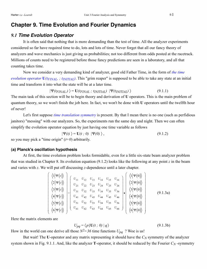
Chapter 9. Time Evolution and Fourier Dynamics
9.1 Time Evolution Operator It is often said that nothing that is more demanding than the test of time. All the analyzer experiments considered so far have required time to do, lots and lots of time. Never forget that all our fancy theory of analyzers and wave mechanics is just giving us probabilities; not too different from odds posted at the racetrack. Millions of counts need to be registered before those fancy predictions are seen in a laboratory, and all that counting takes time. Now we consider a very demanding kind of analyzer, good old Father Time, in the form of the time evolution operator U(tFINAL, ; tINITIAL). This "grim reaper" is supposed to be able to take any state at an initial time and transform it into what the state will be at a later time. |Ψ(tFINAL,) 〉 = U(tFINAL ; tINITIAL) |Ψ(tINITIAL) 〉 (9.1.1)The main task of this section will be to begin theory and derivation of U operators. This is the main problem of quantum theory, so we won't finish the job here. In fact, we won't be done with U operators until the twelfth hour of never! Let's first suppose time translation symmetry is present. By that I mean there is no one (such as perfidious janitors) "messing" with our analyzers. So, the experiments run the same day and night. Then we can often simplify the evolution operator equation by just having one time variable as follows |Ψ(t) 〉 = U(t ; 0) |Ψ(0) 〉 , (9.1.2)so you may pick a "time origin" (t=0) arbitrarily.
(a) Planck's oscillation hypothesis At first, the time evolution problem looks formidable, even for a little six-state beam analyzer problem that was studied in Chapter 8. Its evolution equation (9.1.2) looks like the following at any point z in the beam and varies with z. We will put off discussing z-dependence until a later chapter.
1 Ψ t( )2 Ψ t( )3 Ψ t( )4 Ψ t( )5 Ψ t( )6 Ψ t( )
⎛
⎝
⎜⎜⎜⎜⎜⎜⎜⎜⎜⎜⎜
⎞
⎠
⎟⎟⎟⎟⎟⎟⎟⎟⎟⎟⎟
=
U11 U12 U13 U14 U15 U16
U21 U22 U23 U24 U25 U26
U31 U32 U33 U34 U35 U36
U41 U42 U43 U44 U45 U46
U51 U52 U53 U54 U55 U56
U61 U62 U63 U64 U65 U66
⎛
⎝
⎜⎜⎜⎜⎜⎜⎜⎜⎜
⎞
⎠
⎟⎟⎟⎟⎟⎟⎟⎟⎟
•
1 Ψ 0( )2 Ψ 0( )3 Ψ 0( )4 Ψ 0( )5 Ψ 0( )6 Ψ 0( )
⎛
⎝
⎜⎜⎜⎜⎜⎜⎜⎜⎜⎜⎜
⎞
⎠
⎟⎟⎟⎟⎟⎟⎟⎟⎟⎟⎟
(9.1.3a)
Here the matrix elements are Upq = 〈 p | U(t ; 0) | q 〉 (9.1.3b)How in the world can one derive all those N2=36 time functions Upq ? Woe is us! But wait! The U-operator and any matrix representing it should have the CN symmetry of the analyzer system shown in Fig. 9.1.1. And, like the analyzer T-operator, it should be reduced by the Fourier CN -symmetry
HarterSoft –LearnIt Unit 3 Fourier Analysis and Symmetry 9-1
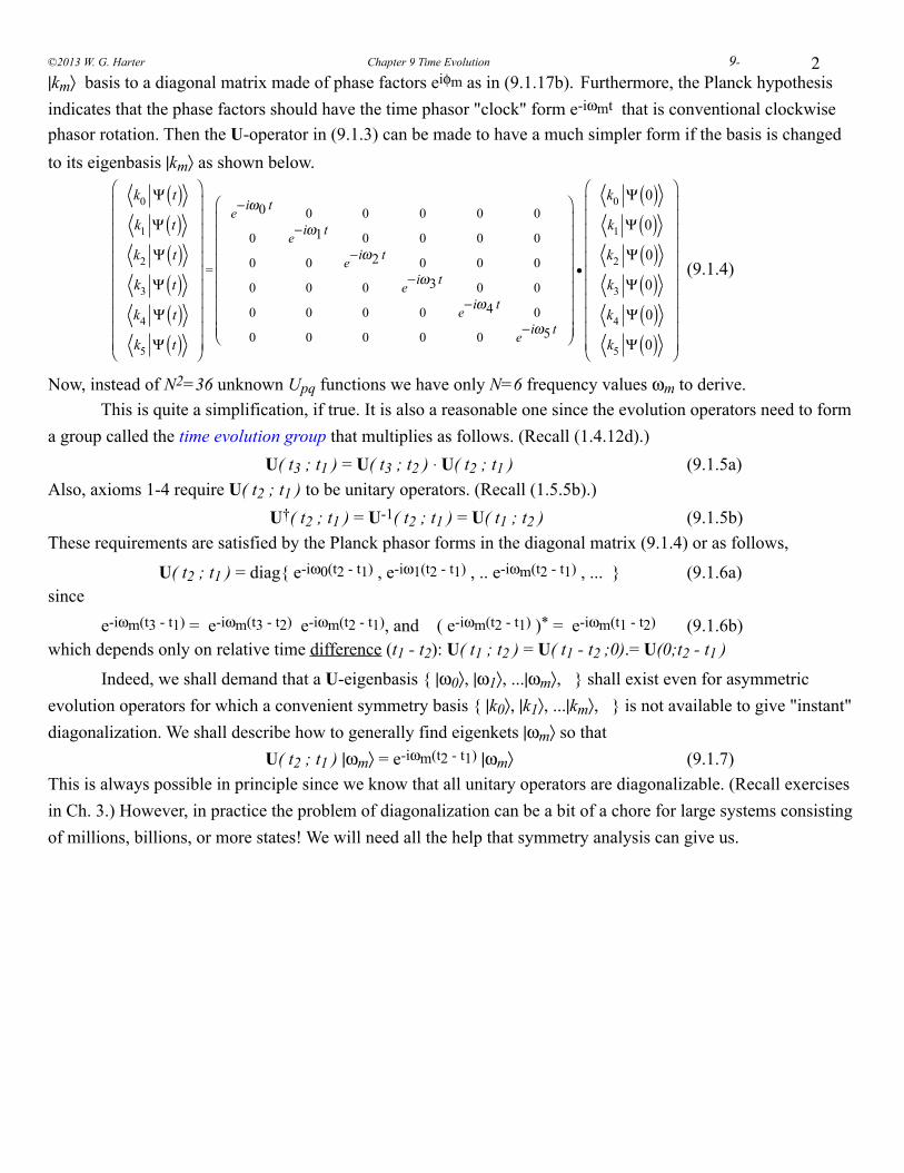
2|km〉 basis to a diagonal matrix made of phase factors eiφm as in (9.1.17b). Furthermore, the Planck hypothesis indicates that the phase factors should have the time phasor "clock" form e-iωmt that is conventional clockwise phasor rotation. Then the U-operator in (9.1.3) can be made to have a much simpler form if the basis is changed to its eigenbasis |km〉 as shown below.
k0 Ψ t( )k1 Ψ t( )k2 Ψ t( )k3 Ψ t( )k4 Ψ t( )k5 Ψ t( )
⎛
⎝
⎜⎜⎜⎜⎜⎜⎜⎜⎜⎜⎜
⎞
⎠
⎟⎟⎟⎟⎟⎟⎟⎟⎟⎟⎟
=
e−iω0 t 0 0 0 0 0
0 e−iω1 t 0 0 0 0
0 0 e−iω2 t 0 0 0
0 0 0 e−iω3 t 0 0
0 0 0 0 e−iω4 t 0
0 0 0 0 0 e−iω5 t
⎛
⎝
⎜⎜⎜⎜⎜⎜⎜⎜⎜
⎞
⎠
⎟⎟⎟⎟⎟⎟⎟⎟⎟
•
k0 Ψ 0( )k1 Ψ 0( )k2 Ψ 0( )k3 Ψ 0( )k4 Ψ 0( )k5 Ψ 0( )
⎛
⎝
⎜⎜⎜⎜⎜⎜⎜⎜⎜⎜⎜
⎞
⎠
⎟⎟⎟⎟⎟⎟⎟⎟⎟⎟⎟
(9.1.4)
Now, instead of N2=36 unknown Upq functions we have only N=6 frequency values ωm to derive. This is quite a simplification, if true. It is also a reasonable one since the evolution operators need to form a group called the time evolution group that multiplies as follows. (Recall (1.4.12d).) U( t3 ; t1 ) = U( t3 ; t2 ) . U( t2 ; t1 ) (9.1.5a)Also, axioms 1-4 require U( t2 ; t1 ) to be unitary operators. (Recall (1.5.5b).) U†( t2 ; t1 ) = U-1( t2 ; t1 ) = U( t1 ; t2 ) (9.1.5b)These requirements are satisfied by the Planck phasor forms in the diagonal matrix (9.1.4) or as follows,
U( t2 ; t1 ) = diag{ e-iω0(t2 - t1) , e-iω1(t2 - t1) , .. e-iωm(t2 - t1) , ... } (9.1.6a)since
e-iωm(t3 - t1) = e-iωm(t3 - t2) e-iωm(t2 - t1), and ( e-iωm(t2 - t1) )* = e-iωm(t1 - t2) (9.1.6b)which depends only on relative time difference (t1 - t2): U( t1 ; t2 ) = U( t1 - t2 ;0).= U(0;t2 - t1 )
Indeed, we shall demand that a U-eigenbasis { |ω0〉, |ω1〉, ...|ωm〉, } shall exist even for asymmetric evolution operators for which a convenient symmetry basis { |k0〉, |k1〉, ...|km〉, } is not available to give "instant" diagonalization. We shall describe how to generally find eigenkets |ωm〉 so that U( t2 ; t1 ) |ωm〉 = e-iωm(t2 - t1) |ωm〉 (9.1.7)This is always possible in principle since we know that all unitary operators are diagonalizable. (Recall exercises in Ch. 3.) However, in practice the problem of diagonalization can be a bit of a chore for large systems consisting of millions, billions, or more states! We will need all the help that symmetry analysis can give us.
©2013 W. G. Harter Chapter 9 Time Evolution 9-
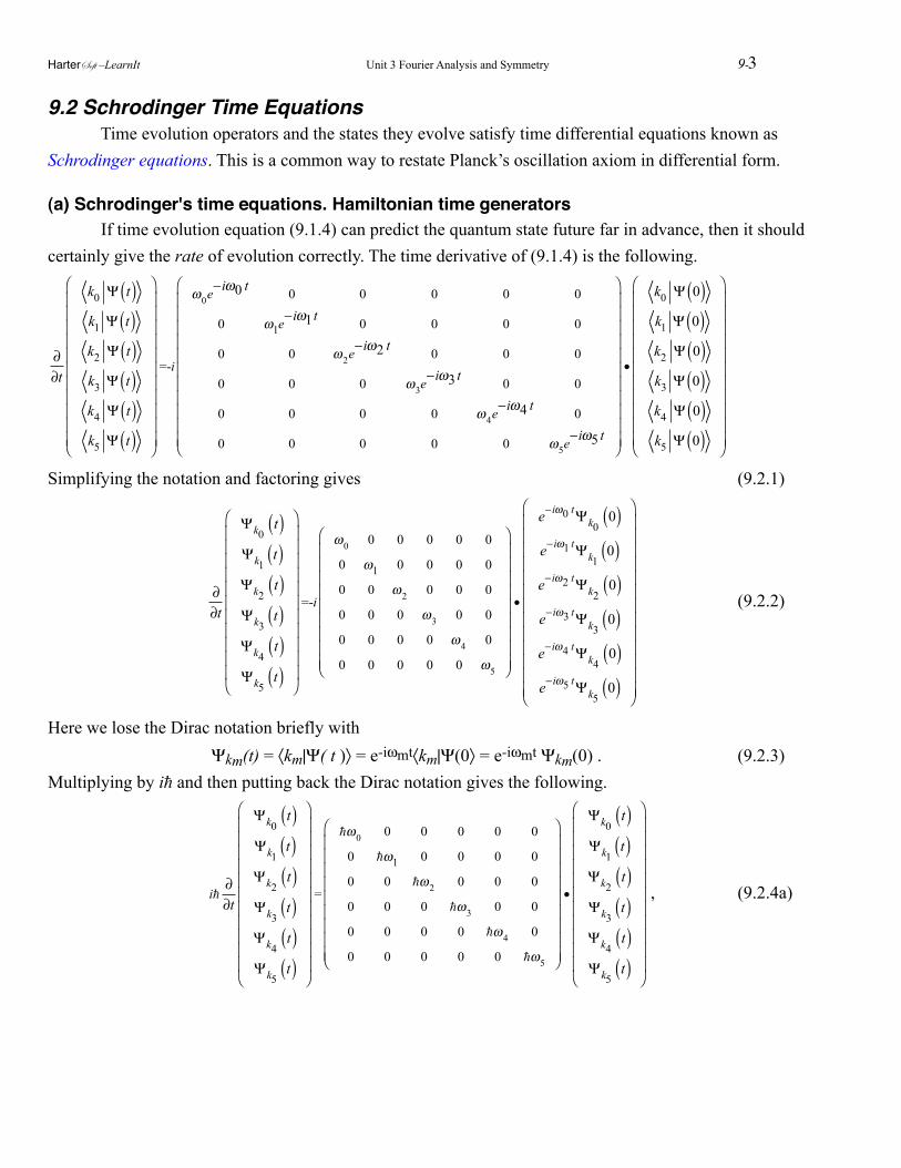
9.2 Schrodinger Time Equations Time evolution operators and the states they evolve satisfy time differential equations known as Schrodinger equations. This is a common way to restate Planck’s oscillation axiom in differential form.
(a) Schrodinger's time equations. Hamiltonian time generators If time evolution equation (9.1.4) can predict the quantum state future far in advance, then it should certainly give the rate of evolution correctly. The time derivative of (9.1.4) is the following.
∂∂t
k0 Ψ t( )k1 Ψ t( )k2 Ψ t( )k3 Ψ t( )k4 Ψ t( )k5 Ψ t( )
⎛
⎝
⎜⎜⎜⎜⎜⎜⎜⎜⎜⎜⎜
⎞
⎠
⎟⎟⎟⎟⎟⎟⎟⎟⎟⎟⎟
=-i
ω0e−iω0 t 0 0 0 0 0
0 ω1e−iω1 t 0 0 0 0
0 0 ω2e−iω2 t 0 0 0
0 0 0 ω3e−iω3 t 0 0
0 0 0 0 ω4e−iω4 t 0
0 0 0 0 0 ω5e−iω5 t
⎛
⎝
⎜⎜⎜⎜⎜⎜⎜⎜⎜⎜⎜
⎞
⎠
⎟⎟⎟⎟⎟⎟⎟⎟⎟⎟⎟
•
k0 Ψ 0( )k1 Ψ 0( )k2 Ψ 0( )k3 Ψ 0( )k4 Ψ 0( )k5 Ψ 0( )
⎛
⎝
⎜⎜⎜⎜⎜⎜⎜⎜⎜⎜⎜
⎞
⎠
⎟⎟⎟⎟⎟⎟⎟⎟⎟⎟⎟
Simplifying the notation and factoring gives (9.2.1)
∂∂t
Ψk0t( )
Ψk1t( )
Ψk2t( )
Ψk3t( )
Ψk4t( )
Ψk5t( )
⎛
⎝
⎜⎜⎜⎜⎜⎜⎜⎜⎜⎜⎜
⎞
⎠
⎟⎟⎟⎟⎟⎟⎟⎟⎟⎟⎟
=-i
ω0 0 0 0 0 0
0 ω1 0 0 0 0
0 0 ω2 0 0 0
0 0 0 ω3 0 0
0 0 0 0 ω4 0
0 0 0 0 0 ω5
⎛
⎝
⎜⎜⎜⎜⎜⎜⎜⎜⎜
⎞
⎠
⎟⎟⎟⎟⎟⎟⎟⎟⎟
•
e−iω0 tΨk00( )
e−iω1 tΨk10( )
e−iω2 tΨk20( )
e−iω3 tΨk30( )
e−iω4 tΨk40( )
e−iω5 tΨk50( )
⎛
⎝
⎜⎜⎜⎜⎜⎜⎜⎜⎜⎜⎜⎜⎜
⎞
⎠
⎟⎟⎟⎟⎟⎟⎟⎟⎟⎟⎟⎟⎟
(9.2.2)
Here we lose the Dirac notation briefly with Ψkm(t) = 〈km|Ψ( t )〉 = e-iωmt〈km|Ψ(0〉 = e-iωmt Ψkm(0) . (9.2.3)Multiplying by i and then putting back the Dirac notation gives the following.
i∂∂t
Ψk0t( )
Ψk1t( )
Ψk2t( )
Ψk3t( )
Ψk4t( )
Ψk5t( )
⎛
⎝
⎜⎜⎜⎜⎜⎜⎜⎜⎜⎜⎜
⎞
⎠
⎟⎟⎟⎟⎟⎟⎟⎟⎟⎟⎟
=
ω0 0 0 0 0 0
0 ω1 0 0 0 0
0 0 ω2 0 0 0
0 0 0 ω3 0 0
0 0 0 0 ω4 0
0 0 0 0 0 ω5
⎛
⎝
⎜⎜⎜⎜⎜⎜⎜⎜⎜
⎞
⎠
⎟⎟⎟⎟⎟⎟⎟⎟⎟
•
Ψk0t( )
Ψk1t( )
Ψk2t( )
Ψk3t( )
Ψk4t( )
Ψk5t( )
⎛
⎝
⎜⎜⎜⎜⎜⎜⎜⎜⎜⎜⎜
⎞
⎠
⎟⎟⎟⎟⎟⎟⎟⎟⎟⎟⎟
, (9.2.4a)
HarterSoft –LearnIt Unit 3 Fourier Analysis and Symmetry 9-3
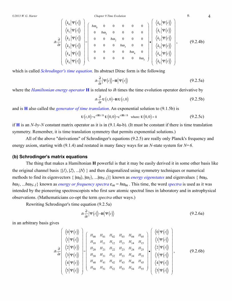
4
i∂∂t
k0 Ψ t( )k1 Ψ t( )k2 Ψ t( )k3 Ψ t( )k4 Ψ t( )k5 Ψ t( )
⎛
⎝
⎜⎜⎜⎜⎜⎜⎜⎜⎜⎜⎜
⎞
⎠
⎟⎟⎟⎟⎟⎟⎟⎟⎟⎟⎟
=
ω0 0 0 0 0 0
0 ω1 0 0 0 0
0 0 ω2 0 0 0
0 0 0 ω3 0 0
0 0 0 0 ω4 0
0 0 0 0 0 ω5
⎛
⎝
⎜⎜⎜⎜⎜⎜⎜⎜⎜
⎞
⎠
⎟⎟⎟⎟⎟⎟⎟⎟⎟
•
k0 Ψ t( )k1 Ψ t( )k2 Ψ t( )k3 Ψ t( )k4 Ψ t( )k5 Ψ t( )
⎛
⎝
⎜⎜⎜⎜⎜⎜⎜⎜⎜⎜⎜
⎞
⎠
⎟⎟⎟⎟⎟⎟⎟⎟⎟⎟⎟
, (9.2.4b)
which is called Schrodinger's time equation. Its abstract Dirac form is the following
i
∂∂t
Ψ t( ) =H Ψ t( ) (9.2.5a)
where the Hamiltonian energy operator H is related to i times the time evolution operator derivative by
i
∂∂t
U t,0( )=H U t,0( ) (9.2.5b)
and is H also called the generator of time translation. An exponential solution to (9.1.5b) is
U t,0( )=e-i H t / U 0,0( )=e-i H t / where: U 0,0( ) = 1 (9.2.5c)
if H is an N-by-N constant matrix operator as it is in (9.1.4a-b). (It must be constant if there is time translation symmetry. Remember, it is time translation symmetry that permits exponential solutions.) All of the above "derivations" of Schrodinger's equations (9.2.5) are really only Planck's frequency and energy axiom, starting with (9.1.4) and restated in many fancy ways for an N-state system for N=6.
(b) Schrodinger's matrix equations The thing that makes a Hamiltonian H powerful is that it may be easily derived it in some other basis like the original channel basis {|1〉, |2〉, ...|N〉 } and then diagonalized using symmetry techniques or numerical methods to find its eigenvectors { |ω0〉, |ω1〉, ...|ωN-1〉} known as energy eigenstates and eigenvalues { ω0, ω1, ...ωN-1} known as energy or frequency spectra εm = ωm . This time, the word spectra is used as it was intended by the pioneering spectroscopists who first saw atomic spectral lines in laboratory and in astrophysical observations. (Mathematicians co-opt the term spectra other ways.) Rewriting Schrodinger's time equation (9.2.5a)
i
∂∂t
Ψ t( ) =H Ψ t( ) (9.2.6a)
in an arbitrary basis gives
i∂∂t
0 Ψ t( )1 Ψ t( )2 Ψ t( )3 Ψ t( )4 Ψ t( )5 Ψ t( )
⎛
⎝
⎜⎜⎜⎜⎜⎜⎜⎜⎜⎜⎜
⎞
⎠
⎟⎟⎟⎟⎟⎟⎟⎟⎟⎟⎟
=
H00 H01 H02 H03 H04 H05
H10 H11 H12 H13 H14 H15
H20 H21 H22 H23 H24 H25
H30 H31 H32 H33 H34 H35
H40 H41 H42 H43 H44 H45
H50 H51 H52 H53 H54 H55
⎛
⎝
⎜⎜⎜⎜⎜⎜⎜⎜⎜
⎞
⎠
⎟⎟⎟⎟⎟⎟⎟⎟⎟
•
0 Ψ t( )1 Ψ t( )2 Ψ t( )3 Ψ t( )4 Ψ t( )5 Ψ t( )
⎛
⎝
⎜⎜⎜⎜⎜⎜⎜⎜⎜⎜⎜
⎞
⎠
⎟⎟⎟⎟⎟⎟⎟⎟⎟⎟⎟
, (9.2.6b)
©2013 W. G. Harter Chapter 9 Time Evolution 9-
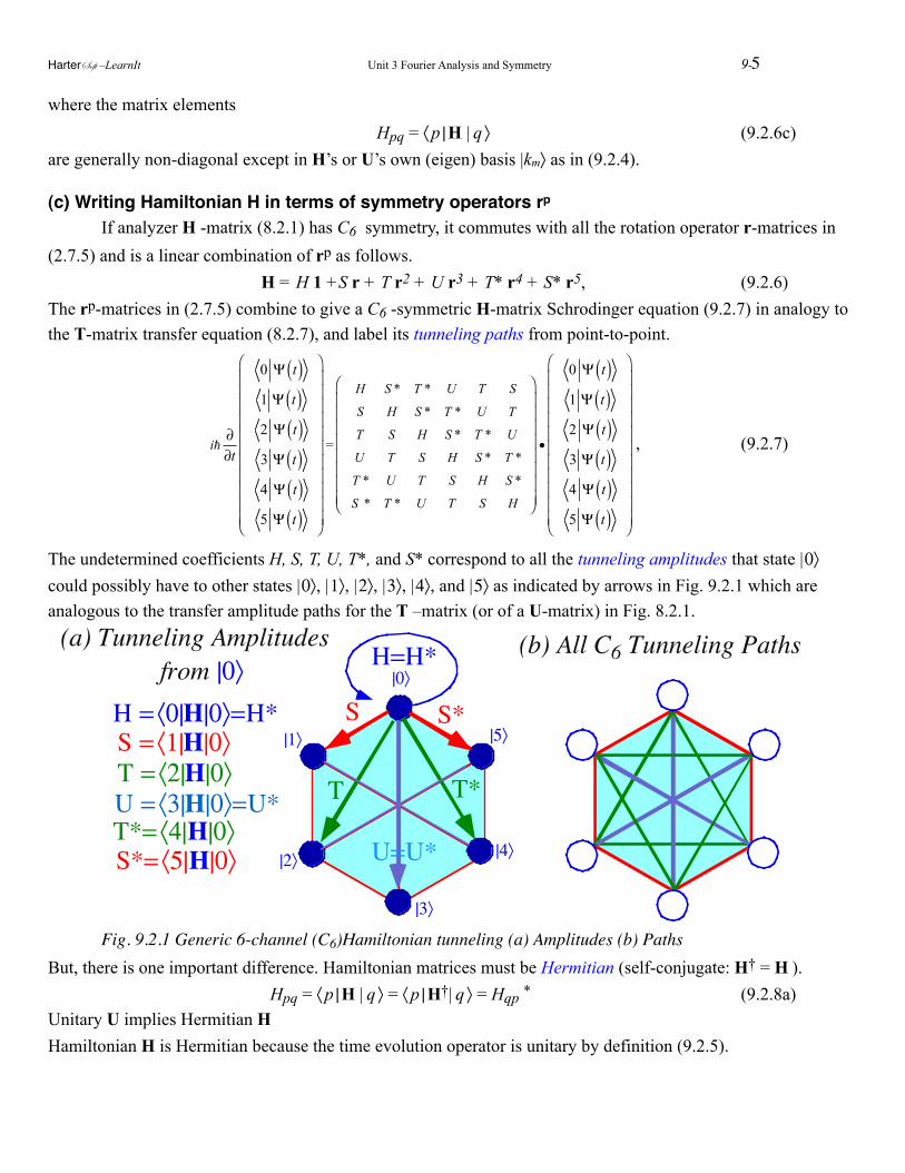
where the matrix elements Hpq = 〈 p | H | q 〉 (9.2.6c)are generally non-diagonal except in H’s or U’s own (eigen) basis |km〉 as in (9.2.4).
(c) Writing Hamiltonian H in terms of symmetry operators rp If analyzer H -matrix (8.2.1) has C6 symmetry, it commutes with all the rotation operator r-matrices in (2.7.5) and is a linear combination of rp as follows. H = H 1 +S r + T r2 + U r3 + T* r4 + S* r5, (9.2.6) The rp-matrices in (2.7.5) combine to give a C6 -symmetric H-matrix Schrodinger equation (9.2.7) in analogy to the T-matrix transfer equation (8.2.7), and label its tunneling paths from point-to-point.
i∂∂t
0 Ψ t( )1 Ψ t( )2 Ψ t( )3 Ψ t( )4 Ψ t( )5 Ψ t( )
⎛
⎝
⎜⎜⎜⎜⎜⎜⎜⎜⎜⎜⎜
⎞
⎠
⎟⎟⎟⎟⎟⎟⎟⎟⎟⎟⎟
=
H S * T * U T S
S H S * T * U T
T S H S * T * U
U T S H S * T *
T * U T S H S *
S * T * U T S H
⎛
⎝
⎜⎜⎜⎜⎜⎜⎜⎜
⎞
⎠
⎟⎟⎟⎟⎟⎟⎟⎟
•
0 Ψ t( )1 Ψ t( )2 Ψ t( )3 Ψ t( )4 Ψ t( )5 Ψ t( )
⎛
⎝
⎜⎜⎜⎜⎜⎜⎜⎜⎜⎜⎜
⎞
⎠
⎟⎟⎟⎟⎟⎟⎟⎟⎟⎟⎟
, (9.2.7)
The undetermined coefficients H, S, T, U, T*, and S* correspond to all the tunneling amplitudes that state |0〉 could possibly have to other states |0〉, |1〉, |2〉, |3〉, |4〉, and |5〉 as indicated by arrows in Fig. 9.2.1 which are analogous to the transfer amplitude paths for the T –matrix (or of a U-matrix) in Fig. 8.2.1.
|0〉H=H*
S S*
T T*
U=U*
|1〉
|2〉
|3〉
|4〉
|5〉
(a) Tunneling Amplitudes from |0〉
S = 〈1|H|0〉H = 〈0|H|0〉=H*
T = 〈2|H|0〉U = 〈3|H|0〉=U*T*= 〈4|H|0〉S*= 〈5|H|0〉
(b) All C6 Tunneling Paths
! Fig. 9.2.1 Generic 6-channel (C6)Hamiltonian tunneling (a) Amplitudes (b) PathsBut, there is one important difference. Hamiltonian matrices must be Hermitian (self-conjugate: H† = H ). Hpq = 〈 p | H | q 〉 = 〈 p | H†| q 〉 = Hqp * (9.2.8a)Unitary U implies Hermitian HHamiltonian H is Hermitian because the time evolution operator is unitary by definition (9.2.5).
HarterSoft –LearnIt Unit 3 Fourier Analysis and Symmetry 9-5
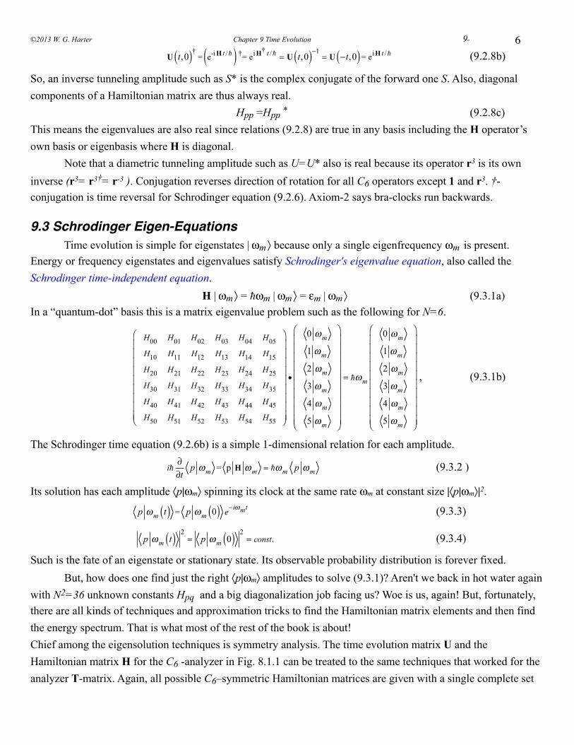
6
U t,0( )† = e-i H t /( ) †= ei H† t / = U t,0( )−1
= U −t,0( )= ei H t / (9.2.8b)
So, an inverse tunneling amplitude such as S* is the complex conjugate of the forward one S. Also, diagonal components of a Hamiltonian matrix are thus always real. Hpp =Hpp * (9.2.8c)This means the eigenvalues are also real since relations (9.2.8) are true in any basis including the H operator’s own basis or eigenbasis where H is diagonal. Note that a diametric tunneling amplitude such as U=U* also is real because its operator r3 is its own inverse (r3= r3†= r-3 ). Conjugation reverses direction of rotation for all C6 operators except 1 and r3. †-conjugation is time reversal for Schrodinger equation (9.2.6). Axiom-2 says bra-clocks run backwards.
9.3 Schrodinger Eigen-Equations Time evolution is simple for eigenstates | ωm 〉 because only a single eigenfrequency ωm is present. Energy or frequency eigenstates and eigenvalues satisfy Schrodinger's eigenvalue equation, also called the Schrodinger time-independent equation. H | ωm 〉 = ωm | ωm 〉 = εm | ωm 〉 (9.3.1a)In a “quantum-dot” basis this is a matrix eigenvalue problem such as the following for N=6.
H00 H01 H02 H03 H04 H05
H10 H11 H12 H13 H14 H15
H20 H21 H22 H23 H24 H25
H30 H31 H32 H33 H34 H35
H40 H41 H42 H43 H44 H45
H50 H51 H52 H53 H54 H55
⎛
⎝
⎜⎜⎜⎜⎜⎜⎜⎜⎜
⎞
⎠
⎟⎟⎟⎟⎟⎟⎟⎟⎟
•
0 ωm
1 ωm
2 ωm
3 ωm
4 ωm
5 ωm
⎛
⎝
⎜⎜⎜⎜⎜⎜⎜⎜⎜⎜
⎞
⎠
⎟⎟⎟⎟⎟⎟⎟⎟⎟⎟
= ωm
0 ωm
1 ωm
2 ωm
3 ωm
4 ωm
5 ωm
⎛
⎝
⎜⎜⎜⎜⎜⎜⎜⎜⎜⎜
⎞
⎠
⎟⎟⎟⎟⎟⎟⎟⎟⎟⎟
, (9.3.1b)
The Schrodinger time equation (9.2.6b) is a simple 1-dimensional relation for each amplitude.
i
∂∂t
p ωm = p H ωm = ωm p ωm (9.3.2 )
Its solution has each amplitude 〈p|ωm〉 spinning its clock at the same rate ωm at constant size |〈p|ωm〉|2.
p ωm t( ) = p ωm 0( ) e−iωmt (9.3.3)
p ωm t( ) 2
= p ωm 0( ) 2= const. (9.3.4)
Such is the fate of an eigenstate or stationary state. Its observable probability distribution is forever fixed. But, how does one find just the right 〈p|ωm〉 amplitudes to solve (9.3.1)? Aren't we back in hot water again with N2=36 unknown constants Hpq and a big diagonalization job facing us? Woe is us, again! But, fortunately, there are all kinds of techniques and approximation tricks to find the Hamiltonian matrix elements and then find the energy spectrum. That is what most of the rest of the book is about! Chief among the eigensolution techniques is symmetry analysis. The time evolution matrix U and the Hamiltonian matrix H for the C6 -analyzer in Fig. 8.1.1 can be treated to the same techniques that worked for the analyzer T-matrix. Again, all possible C6–symmetric Hamiltonian matrices are given with a single complete set
©2013 W. G. Harter Chapter 9 Time Evolution 9-
of eigensolutions. Then all possible motions are obtained from combinations of eigensolutions, which, by their completeness are able to produce an arbitrary initial condition. After that, the motion is just the interference beating between all the eigenfrequencies that participate in producing a given initial state. Remember, it takes two to tango! At least two eigenstates with different eigenfrequencies need to be up and spinning to have observable motion. Otherwise, nothin’s happening!It turns out that while it takes two to tango, three’s a crowd! Two state systems are unique in their harmonic simplicity. At the end of this unit we will see how to understand more complicated 3, 4, 5,…level excitations for some simple systems.
HarterSoft –LearnIt Unit 3 Fourier Analysis and Symmetry 9-7
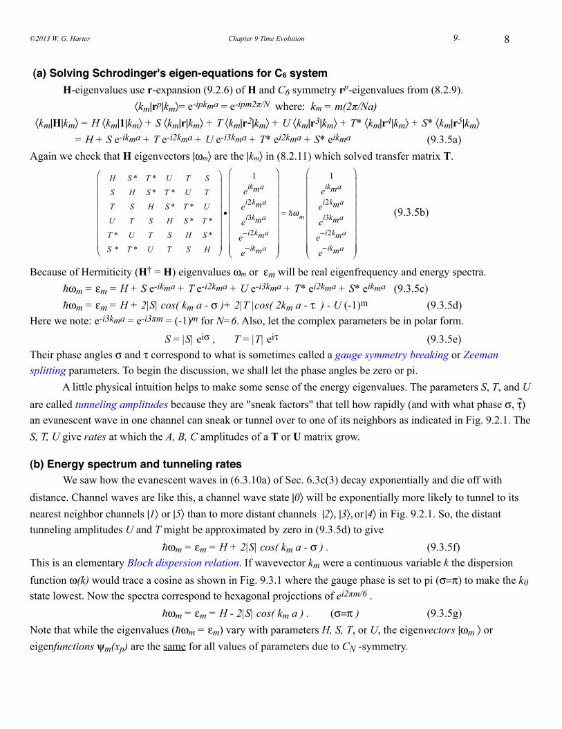
8
(a) Solving Schrodinger's eigen-equations for C6 system H-eigenvalues use r-expansion (9.2.6) of H and C6 symmetry rp-eigenvalues from (8.2.9). 〈km|rp|km〉= e-ipkma = e-ipm2π/N where: km = m(2π/Na) 〈km|H|km〉 = H 〈km|1|km〉 + S 〈km|r|km〉 + T 〈km|r2|km〉 + U 〈km|r3|km〉 + T* 〈km|r4|km〉 + S* 〈km|r5|km〉6 = H + S e-ikma + T e-i2kma + U e-i3kma + T* ei2kma + S* eikma (9.3.5a) Again we check that H eigenvectors |ωm〉 are the |km〉 in (8.2.11) which solved transfer matrix T.
H S * T * U T S
S H S * T * U T
T S H S * T * U
U T S H S * T *
T * U T S H S *
S * T * U T S H
⎛
⎝
⎜⎜⎜⎜⎜⎜⎜⎜
⎞
⎠
⎟⎟⎟⎟⎟⎟⎟⎟
•
1
eikma
ei2kma
ei3kma
e−i2kma
e−ikma
⎛
⎝
⎜⎜⎜⎜⎜⎜⎜⎜⎜
⎞
⎠
⎟⎟⎟⎟⎟⎟⎟⎟⎟
= ωm
1
eikma
ei2kma
ei3kma
e−i2kma
e−ikma
⎛
⎝
⎜⎜⎜⎜⎜⎜⎜⎜⎜
⎞
⎠
⎟⎟⎟⎟⎟⎟⎟⎟⎟
(9.3.5b)
Because of Hermiticity (H† = H) eigenvalues ωm or εm will be real eigenfrequency and energy spectra. ωm = εm = H + S e-ikma + T e-i2kma + U e-i3kma + T* ei2kma + S* eikma (9.3.5c) ωm = εm = H + 2|S| cos( km a - σ )+ 2|T |cos( 2km a - τ ) - U (-1)m (9.3.5d) Here we note: e-i3kma = e-i3πm = (-1)m for N=6. Also, let the complex parameters be in polar form.
S = |S| eiσ , T = |T| eiτ (9.3.5e) Their phase angles σ and τ correspond to what is sometimes called a gauge symmetry breaking or Zeeman splitting parameters. To begin the discussion, we shall let the phase angles be zero or pi. A little physical intuition helps to make some sense of the energy eigenvalues. The parameters S, T, and U are called tunneling amplitudes because they are "sneak factors" that tell how rapidly (and with what phase σ, τ) an evanescent wave in one channel can sneak or tunnel over to one of its neighbors as indicated in Fig. 9.2.1. The S, T, U give rates at which the A, B, C amplitudes of a T or U matrix grow.
(b) Energy spectrum and tunneling rates We saw how the evanescent waves in (6.3.10a) of Sec. 6.3c(3) decay exponentially and die off with distance. Channel waves are like this, a channel wave state |0〉 will be exponentially more likely to tunnel to its nearest neighbor channels |1〉 or |5〉 than to more distant channels |2〉, |3〉, or |4〉 in Fig. 9.2.1. So, the distant tunneling amplitudes U and T might be approximated by zero in (9.3.5d) to give ωm = εm = H + 2|S| cos( km a - σ ) . (9.3.5f) This is an elementary Bloch dispersion relation. If wavevector km were a continuous variable k the dispersion function ω(k) would trace a cosine as shown in Fig. 9.3.1 where the gauge phase is set to pi (σ=π) to make the k0 state lowest. Now the spectra correspond to hexagonal projections of ei2πm/6 . ωm = εm = H - 2|S| cos( km a ) . (σ=π ) (9.3.5g) Note that while the eigenvalues (ωm = εm) vary with parameters H, S, T, or U, the eigenvectors |ωm 〉 or eigenfunctions ψm(xp) are the same for all values of parameters due to CN -symmetry.
©2013 W. G. Harter Chapter 9 Time Evolution 9-
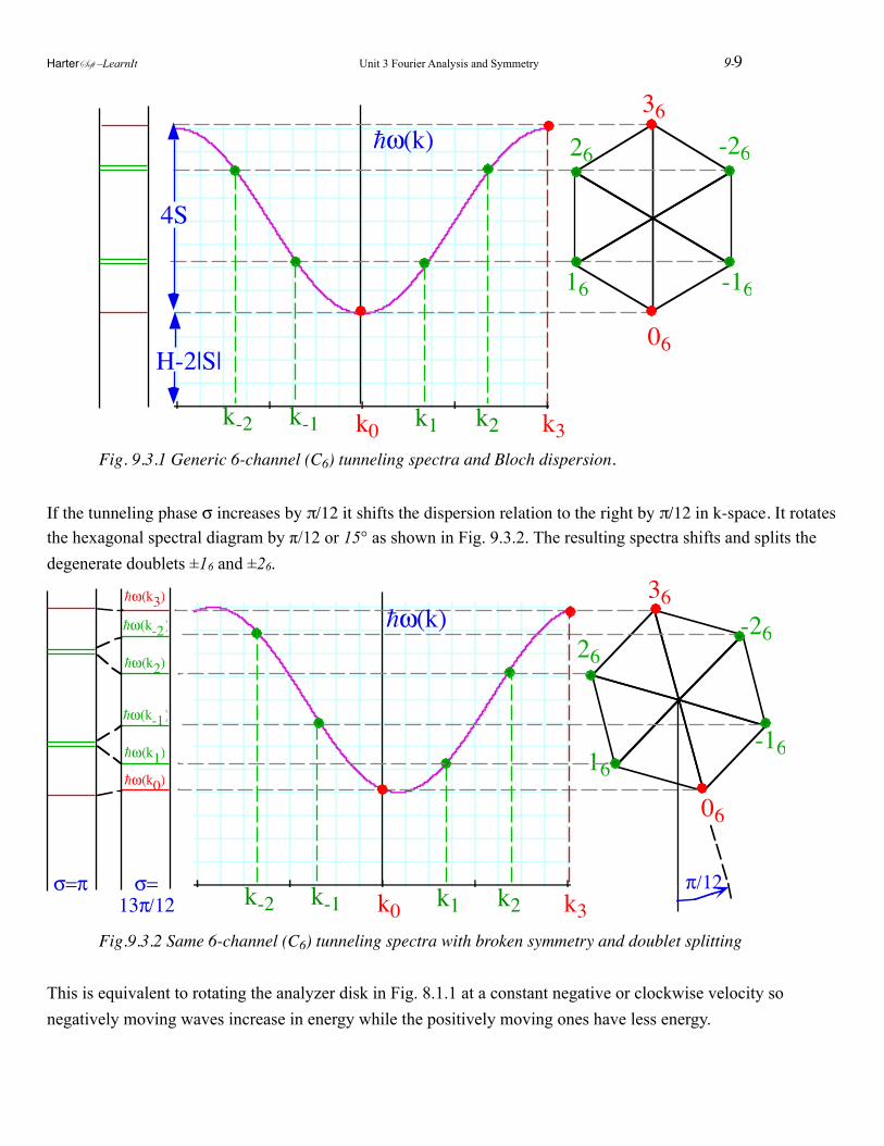
!
ω(k)
k0k-2 k-1 k1 k2 k3
06
36
-2626
-1616
4S
H-2|S|
! Fig. 9.3.1 Generic 6-channel (C6) tunneling spectra and Bloch dispersion.
If the tunneling phase σ increases by π/12 it shifts the dispersion relation to the right by π/12 in k-space. It rotates the hexagonal spectral diagram by π/12 or 15° as shown in Fig. 9.3.2. The resulting spectra shifts and splits the degenerate doublets ±16 and ±26.
ω(k)
k0k-2 k-1 k1 k2 k3
06
36-2626
-1616
σ=π σ=13π/12
π/12
ω(k0)
ω(k3)
ω(k-2)
ω(k2)
ω(k-1)
ω(k1)
! Fig.9.3.2 Same 6-channel (C6) tunneling spectra with broken symmetry and doublet splitting
This is equivalent to rotating the analyzer disk in Fig. 8.1.1 at a constant negative or clockwise velocity so negatively moving waves increase in energy while the positively moving ones have less energy.
HarterSoft –LearnIt Unit 3 Fourier Analysis and Symmetry 9-9
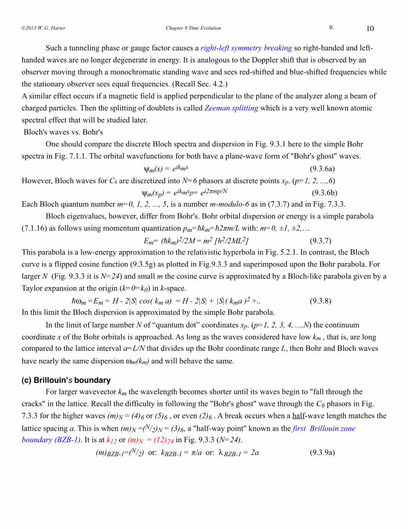
10
Such a tunneling phase or gauge factor causes a right-left symmetry breaking so right-handed and left-handed waves are no longer degenerate in energy. It is analogous to the Doppler shift that is observed by an observer moving through a monochromatic standing wave and sees red-shifted and blue-shifted frequencies while the stationary observer sees equal frequencies. (Recall Sec. 4.2.)A similar effect occurs if a magnetic field is applied perpendicular to the plane of the analyzer along a beam of charged particles. Then the splitting of doublets is called Zeeman splitting which is a very well known atomic spectral effect that will be studied later. Bloch's waves vs. Bohr's One should compare the discrete Bloch spectra and dispersion in Fig. 9.3.1 here to the simple Bohr spectra in Fig. 7.1.1. The orbital wavefunctions for both have a plane-wave form of "Bohr's ghost" waves.
ψm(x) = eikmx (9.3.6a)However, Bloch waves for C6 are discretized into N=6 phasors at discrete points xp. (p=1, 2, ...,6) ψm(xp) = eikmxp= ei2πmp/N (9.3.6b)Each Bloch quantum number m=0, 1, 2, ..., 5, is a number m-modulo-6 as in (7.3.7) and in Fig. 7.3.3. Bloch eigenvalues, however, differ from Bohr's. Bohr orbital dispersion or energy is a simple parabola (7.1.16) as follows using momentum quantization pm=km=2πm/L with: m=0, ±1, ±2,…
Em= (km)2/2M = m2 [h2/2ML2] (9.3.7)This parabola is a low-energy approximation to the relativistic hyperbola in Fig. 5.2.1. In contrast, the Bloch curve is a flipped cosine function (9.3.5g) as plotted in Fig.9.3.3 and superimposed upon the Bohr parabola. For larger N (Fig. 9.3.3 it is N=24) and small m the cosine curve is approximated by a Bloch-like parabola given by a Taylor expansion at the origin (k=0=k0) in k-space. ωm =Em = H - 2|S| cos( km a) = H - 2|S| + |S|( kma )2 +.. (9.3.8)In this limit the Bloch dispersion is approximated by the simple Bohr parabola. In the limit of large number N of “quantum dot” coordinates xp. (p=1, 2, 3, 4, ...,N) the continuum coordinate x of the Bohr orbitals is approached. As long as the waves considered have low km , that is, are long compared to the lattice interval a=L/N that divides up the Bohr coordinate range L, then Bohr and Bloch waves have nearly the same dispersion ωm(km) and will behave the same.
(c) Brillouin's boundary For larger wavevector km the wavelength becomes shorter until its waves begin to "fall through the cracks" in the lattice. Recall the difficulty in following the "Bohr's ghost" wave through the C6 phasors in Fig. 7.3.3 for the higher waves (m)N = (4)6 or (5)6 , or even (2)6 . A break occurs when a half-wave length matches the lattice spacing a. This is when (m)N =(N/2)N = (3)6, a "half-way point" known as the first Brillouin zone boundary (BZB-1). It is at k12 or (m)N = (12)24 in Fig. 9.3.3 (N=24). (m)BZB-1=(N/2) or: kBZB-1 = π/a or: λ BZB-1 = 2a (9.3.9a)
©2013 W. G. Harter Chapter 9 Time Evolution 9-
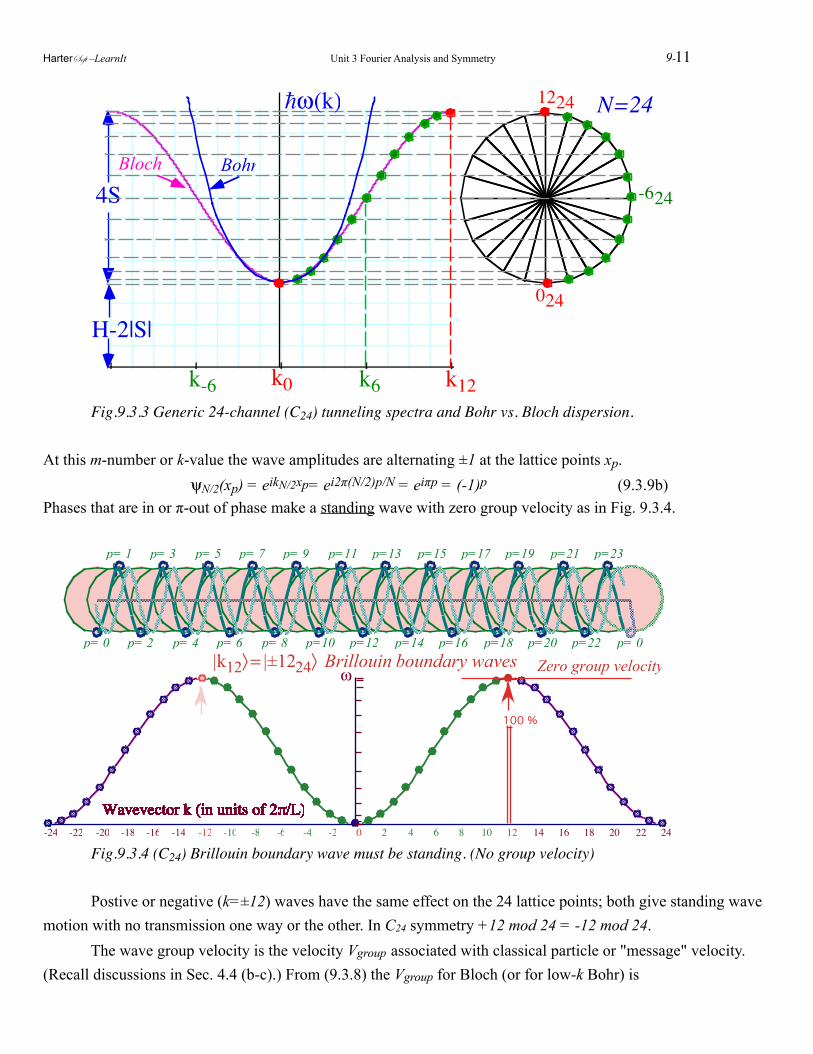
!
4S
H-2|S|
ω(k)
k0 k12k6k-6
N=24
024
1224
-624
BohrBloch
! Fig.9.3.3 Generic 24-channel (C24) tunneling spectra and Bohr vs. Bloch dispersion.
At this m-number or k-value the wave amplitudes are alternating ±1 at the lattice points xp. ψN/2(xp) = eikN/2xp= ei2π(N/2)p/N = eiπp = (-1)p (9.3.9b)Phases that are in or π-out of phase make a standing wave with zero group velocity as in Fig. 9.3.4.
-24
Wavevector k (in units of 2π/L)Wavevector k (in units of 2π/L)-22
Wavevector k (in units of 2π/L)Wavevector k (in units of 2π/L)-20
Wavevector k (in units of 2π/L)Wavevector k (in units of 2π/L)-18
Wavevector k (in units of 2π/L)Wavevector k (in units of 2π/L)-16
Wavevector k (in units of 2π/L)Wavevector k (in units of 2π/L)-14
Wavevector k (in units of 2π/L)Wavevector k (in units of 2π/L)-12
Wavevector k (in units of 2π/L)Wavevector k (in units of 2π/L)-10
Wavevector k (in units of 2π/L)Wavevector k (in units of 2π/L) -8
Wavevector k (in units of 2π/L)Wavevector k (in units of 2π/L) -6
Wavevector k (in units of 2π/L)Wavevector k (in units of 2π/L) -4
Wavevector k (in units of 2π/L)Wavevector k (in units of 2π/L) -2
Wavevector k (in units of 2π/L)Wavevector k (in units of 2π/L) 0
Wavevector k (in units of 2π/L)Wavevector k (in units of 2π/L) 2
Wavevector k (in units of 2π/L)Wavevector k (in units of 2π/L) 4
Wavevector k (in units of 2π/L)Wavevector k (in units of 2π/L) 6
Wavevector k (in units of 2π/L)Wavevector k (in units of 2π/L) 8
Wavevector k (in units of 2π/L)Wavevector k (in units of 2π/L) 10
Wavevector k (in units of 2π/L)Wavevector k (in units of 2π/L) 12
Wavevector k (in units of 2π/L)
100 %
Wavevector k (in units of 2π/L) 14
Wavevector k (in units of 2π/L)Wavevector k (in units of 2π/L) 16
Wavevector k (in units of 2π/L)Wavevector k (in units of 2π/L) 18
Wavevector k (in units of 2π/L)Wavevector k (in units of 2π/L) 20
Wavevector k (in units of 2π/L)Wavevector k (in units of 2π/L) 22
Wavevector k (in units of 2π/L)Wavevector k (in units of 2π/L) 24
Wavevector k (in units of 2π/L)
ω
p= 1 p= 3 p= 5 p= 7 p= 9 p=11 p=13 p=15 p=17 p=19 p=21 p=23
k=12p= 0 p= 2 p= 4 p= 6 p= 8 p=10 p=12 p=14 p=16 p=18 p=20 p=22 p= 0
|k12〉 = |±1224〉 Brillouin boundary waves Zero group velocity
! Fig.9.3.4 (C24) Brillouin boundary wave must be standing. (No group velocity)
Postive or negative (k=±12) waves have the same effect on the 24 lattice points; both give standing wave motion with no transmission one way or the other. In C24 symmetry +12 mod 24 = -12 mod 24. The wave group velocity is the velocity Vgroup associated with classical particle or "message" velocity. (Recall discussions in Sec. 4.4 (b-c).) From (9.3.8) the Vgroup for Bloch (or for low-k Bohr) is
HarterSoft –LearnIt Unit 3 Fourier Analysis and Symmetry 9-11
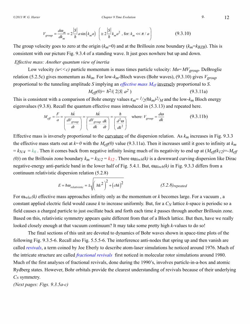
12
Vgroup =dωmdkm
= 2S
a sin kma( ) ≅ 2
S
kma2 , for: km << π / a
⎛
⎝⎜
⎞
⎠⎟ (9.3.10)
The group velocity goes to zero at the origin (km=0) and at the Brillouin zone boundary (km=kBZB). This is consistent with our picture Fig. 9.3.4 of a standing wave. It just goes nowhere but up and down.
Effective mass: Another quantum view of inertia Low velocity (u<<c) particle momentum is mass times particle velocity: Mu=MVgroup. DeBroglie relation (5.2.5c) gives momentum as km. For low-km-Bloch waves (Bohr waves), (9.3.10) gives Vgroup proportional to the tunneling amplitude S implying an effective mass Meff inversely proportional to S. Meff(0)= 2/( 2|S| a2 ) (9.3.11a)This is consistent with a comparison of Bohr energy values εm= 1/2(km)2/M and the low-km Bloch energy eigenvalues (9.3.8). Recall the quantum effective mass introduced in (5.3.13) and repeated here.
Meff = Fa= k
dVgroup
dt
⎛
⎝⎜
⎞
⎠⎟
= kdVgroup
dkdkdt
⎛
⎝⎜
⎞
⎠⎟
=
d2ωdk2
⎛
⎝⎜
⎞
⎠⎟
where: Vgroup = dω
dk (9.3.11b)
Effective mass is inversely proportional to the curvature of the dispersion relation. As km increases in Fig. 9.3.3 the effective mass starts out at k=0 with the Meff(0) value (9.3.11a). Then it increases until it goes to infinity at km = kN/4 = k6 . Then it comes back from negative infinity losing much of its negativity to end up at (Meff(k12)=-Meff
(0)) on the Brillouin zone boundary km = kN/2 = k12 . There ωBloch(k) is a downward curving dispersion like Dirac negative-energy anti-particle band in the lower half of Fig. 5.4.1. But, ωBloch(k) in Fig. 9.3.3 differs from a continuum relativistic dispersion relation (5.2.8)
E = ωrelativistic = ± Mc2⎛
⎝⎜⎞⎠⎟
2+ ck( )2 (5.2.8)repeated
For ωrela.(k) effective mass approaches infinity only as the momentum or k becomes large. For a vacuum , a constant applied electric field would cause k to increase uniformly. But, for a CN lattice k-space is periodic so a field causes a charged particle to just oscillate back and forth each time k passes through another Brillouin zone. Based on this, relativistic symmetry appears quite different from that of a Bloch lattice. But then, have we really looked closely enough at that vacuum continuum? It may take some pretty high k-values to do so! The final sections of this unit are devoted to dynamics of Bohr waves shown in space-time plots of the following Fig. 9.3.5-6. Recall also Fig. 5.5.5-6. The interference anti-nodes that spring up and then vanish are called revivals, a term coined by Joe Eberly to describe atom-laser simulations he noticed around 1976. Much of the intricate structure are called fractional revivals first noticed in molecular rotor simulations around 1980. Much of the first analyses of fractional revivals, done during the 1990’s, involves particle-in-a-box and atomic Rydberg states. However, Bohr orbitals provide the clearest understanding of revivals because of their underlying CN symmetry. (Next pages: Figs. 9.3.5a-c)
©2013 W. G. Harter Chapter 9 Time Evolution 9-
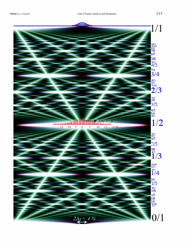
HarterSoft –LearnIt Unit 3 Fourier Analysis and Symmetry 9-13
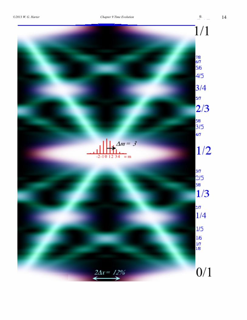
14©2013 W. G. Harter Chapter 9 Time Evolution 9-
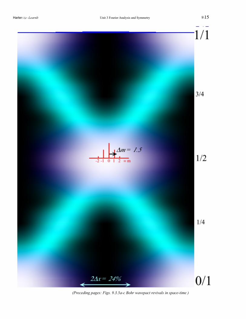
! ! ! ! (Preceding pages: Figs. 9.3.5a-c Bohr wavepact revivals in space-time )
HarterSoft –LearnIt Unit 3 Fourier Analysis and Symmetry 9-15
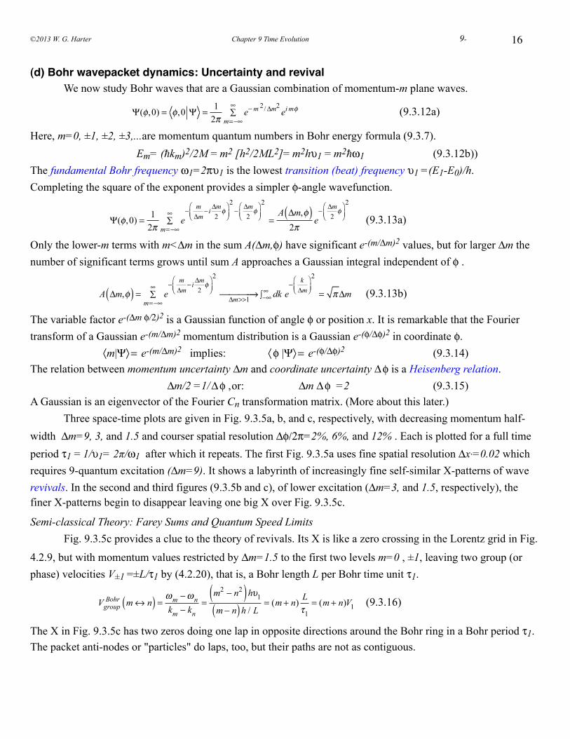
16
(d) Bohr wavepacket dynamics: Uncertainty and revival We now study Bohr waves that are a Gaussian combination of momentum-m plane waves.
Ψ(φ,0) = φ,0 Ψ = 1
2πe− m 2/Δm2
ei mφ
m=−∞
∞∑ (9.3.12a)
Here, m=0, ±1, ±2, ±3,...are momentum quantum numbers in Bohr energy formula (9.3.7). Em= (km)2/2M = m2 [h2/2ML2]= m2hυ1 = m2ω1 (9.3.12b))The fundamental Bohr frequency ω1=2πυ1 is the lowest transition (beat) frequency υ1 =(E1-E0)/h.Completing the square of the exponent provides a simpler φ-angle wavefunction.
Ψ(φ,0) = 1
2πe− m
Δm− iΔm
2φ
⎛⎝⎜
⎞⎠⎟
2− Δm
2φ
⎛⎝⎜
⎞⎠⎟
2
m=−∞
∞∑ =
A Δm,φ( )2π
e− Δm
2φ
⎛⎝⎜
⎞⎠⎟
2
(9.3.13a)
Only the lower-m terms with m<Δm in the sum A(Δm,φ) have significant e-(m/Δm)2 values, but for larger Δm the number of significant terms grows until sum A approaches a Gaussian integral independent of φ .
A Δm,φ( ) = e
− mΔm
− iΔm2φ
⎛⎝⎜
⎞⎠⎟
2
m=−∞
∞∑ Δm>>1
⎯ →⎯⎯⎯ dk−∞∞∫ e
− kΔm
⎛⎝⎜
⎞⎠⎟
2
= πΔm (9.3.13b)
The variable factor e-(Δm φ/2)2 is a Gaussian function of angle φ or position x. It is remarkable that the Fourier transform of a Gaussian e-(m/Δm)2 momentum distribution is a Gaussian e-(φ/Δφ)2 in coordinate φ. 〈m|Ψ〉 = e-(m/Δm)2 implies: 〈 φ |Ψ〉 = e-(φ/Δφ)2 (9.3.14)The relation between momentum uncertainty Δm and coordinate uncertainty Δ φ is a Heisenberg relation. Δm/2 =1/ Δ φ , or: Δm Δ φ =2 (9.3.15)A Gaussian is an eigenvector of the Fourier Cn transformation matrix. (More about this later.) Three space-time plots are given in Fig. 9.3.5a, b, and c, respectively, with decreasing momentum half-width Δm=9, 3, and 1.5 and courser spatial resolution Δφ/2π=2%, 6%, and 12% . Each is plotted for a full time period τ1 = 1/υ1= 2π/ω1 after which it repeats. The first Fig. 9.3.5a uses fine spatial resolution Δx.=0.02 which requires 9-quantum excitation (Δm=9). It shows a labyrinth of increasingly fine self-similar X-patterns of wave revivals. In the second and third figures (9.3.5b and c), of lower excitation (Δm=3, and 1.5, respectively), the finer X-patterns begin to disappear leaving one big X over Fig. 9.3.5c.
Semi-classical Theory: Farey Sums and Quantum Speed Limits Fig. 9.3.5c provides a clue to the theory of revivals. Its X is like a zero crossing in the Lorentz grid in Fig.
4.2.9, but with momentum values restricted by Δm=1.5 to the first two levels m=0 , ±1, leaving two group (or phase) velocities V±1 =±L/τ1 by (4.2.20), that is, a Bohr length L per Bohr time unit τ1.
Vgroup
Bohr m ↔ n( ) = ωm −ωnkm − kn
=m2 − n2( )hυ1
m − n( )h / L= (m + n) L
τ1= (m + n)V1 (9.3.16)
The X in Fig. 9.3.5c has two zeros doing one lap in opposite directions around the Bohr ring in a Bohr period τ1. The packet anti-nodes or "particles" do laps, too, but their paths are not as contiguous.
©2013 W. G. Harter Chapter 9 Time Evolution 9-
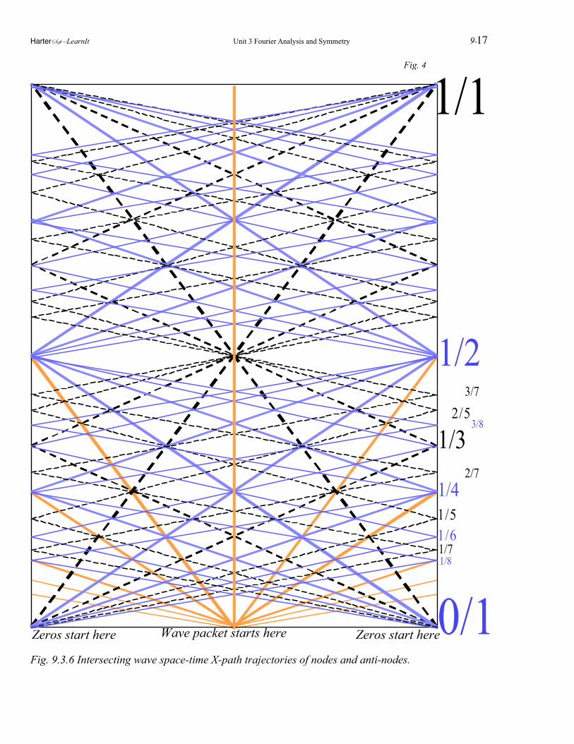
1/2
0/1
1/4
1/1
1/61/7
1/3
1/5
2/5
2/7
3/7
1/8
3/8
Wave packet starts hereZeros start here Zeros start here
Fig. 4
Fig. 9.3.6 Intersecting wave space-time X-path trajectories of nodes and anti-nodes.
HarterSoft –LearnIt Unit 3 Fourier Analysis and Symmetry 9-17
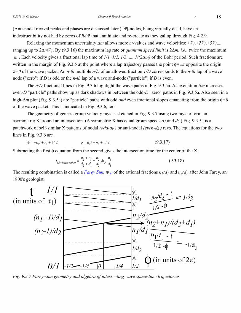
18
(Anti-nodal revival peaks and phases are discussed later.) |Ψ|-nodes, being virtually dead, have an indestructibility not had by zeros of ReΨ that annihilate and re-create as they gallop through Fig. 4.2.9. Relaxing the momentum uncertainty Δm allows more m-values and wave velocities: ±V1,±2V1,±3V1,... ranging up to 2ΔmV1. By (9.3.16) the maximum lap rate or quantum speed limit is 2Δm, i.e., twice the maximum |m|. Each velocity gives a fractional lap time of 1/1, 1/2, 1/3, ..., 1/(2Δm) of the Bohr period. Such fractions are written in the margin of Fig. 9.3.5 at the point where a lap trajectory passes the point φ=±π opposite the origin φ=0 of the wave packet. An n-th multiple n/D of an allowed fraction 1/D corresponds to the n-th lap of a wave node ("zero") if D is odd or the n-th lap of a wave anti-node ("particle") if D is even. The n/D fractional lines in Fig. 9.3.6 highlight the wave paths in Fig. 9.3.5a. As excitation Δm increases, even-D "particle" paths show up as dark shadows in between the odd-D "zero" paths in Fig. 9.3.5a. Also seen in a high-Δm plot (Fig. 9.3.5a) are "particle" paths with odd and even fractional slopes emanating from the origin φ=0 of the wave packet. This is indicated in Fig. 9.3.6, too. The geometry of generic group velocity rays is sketched in Fig. 9.3.7 using two rays to form an asymmetric X around an intersection. (A symmetric X has equal group speeds d1 and d2.) Fig. 9.3.5a is a patchwork of self-similar X patterns of nodal (odd-dk ) or anti-nodal (even-dk ) rays. The equations for the two lines in Fig. 9.3.6 are φ = −d1t + n1 +1 / 2 φ = d2t − n2 +1 / 2 (9.3.17)
Subtracting the first φ equation from the second gives the intersection time for the center of the X.
t12− intersection =
n2 + n1d2 + d1
=n2d2
⊕Fn1d1
(9.3.18)
The resulting combination is called a Farey Sum ⊕ F of the rational fractions n1/d1 and n2/d2 after John Farey, an 1800's geologist.
n2/d2
n1/d1(n2-1)/d2
(n1+1)/d1 (n2+n1)/(d2+d1)
φ
t
0 1/4 1/2
1/d1
1/d2
(in units of 2!)
(in units of τ1)1/1
0/1 -1/2 -1/4
Fig. 9.3.7 Farey-sum geometry and algebra of intersecting wave space-time trajectories.
©2013 W. G. Harter Chapter 9 Time Evolution 9-
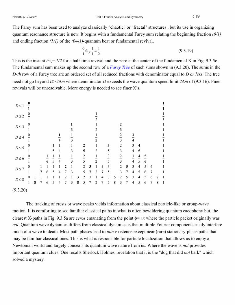
The Farey sum has been used to analyze classically "chaotic" or "fractal" structures , but its use in organizing quantum resonance structure is new. It begins with a fundamental Farey sum relating the beginning fraction (0/1) and ending fraction (1/1) of the (0↔1)-quantum beat or fundamental revival.
01⊕F
11= 1
2 (9.3.19)
This is the instant t/τ1=1/2 for a half-time revival and the zero at the center of the fundamental X in Fig. 9.3.5c. The fundamental sum makes up the second row of a Farey Tree of such sums shown in (9.3.20). The sums in the D-th row of a Farey tree are an ordered set of all reduced fractions with denominator equal to D or less. The tree need not go beyond D>2Δm where denominator D exceeds the wave quantum speed limit 2Δm of (9.3.16). Finer revivals will be unresolvable. More energy is needed to see finer X’s.
D ≤ 1 01
11
D ≤ 2 01
12
11
D ≤ 3 01
13
12
23
11
D ≤ 4 01
14
13
12
23
34
11
D ≤ 5 01
15
14
13
25
12
35
23
34
45
11
D ≤ 6 01
16
15
14
13
25
12
35
23
34
45
56
11
D ≤ 7 01
17
16
15
14
27
13
25
37
12
47
35
23
57
34
45
56
67
11
D ≤ 8 01
18
17
16
15
14
27
13
38
25
37
12
47
35
58
23
57
34
45
56
67
78
11
(9.3.20)
The tracking of crests or wave peaks yields information about classical particle-like or group-wave motion. It is comforting to see familiar classical paths in what is often bewildering quantum cacophony but, the clearest X-paths in Fig. 9.3.5a are zeros emanating from the point φ=±π where the particle packet originally was not. Quantum wave dynamics differs from classical dynamics is that multiple Fourier components easily interfere much of a wave to death. Most path phases lead to non-existence except near (rare) stationary-phase paths that may be familiar classical ones. This is what is responsible for particle localization that allows us to enjoy a Newtonian world and largely conceals its quantum wave nature from us. Where the wave is not provides important quantum clues. One recalls Sherlock Holmes' revelation that it is the "dog that did not bark" which solved a mystery.
HarterSoft –LearnIt Unit 3 Fourier Analysis and Symmetry 9-19
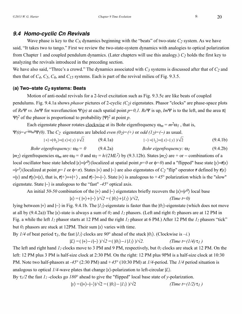
20
9.4 Homo-cyclic Cn Revivals Wave phase is key to the CN dynamics beginning with the “beats” of two-state C2 system. As we have said, “It takes two to tango.” First we review the two-state-system dynamics with analogies to optical polarization from Chapter 1 and coupled pendulum dynamics. (Later chapters will use this analogy.) C2 holds the first key to analyzing the revivals introduced in the preceding section.We have also said, “Three’s a crowd.” The dynamics associated with C3 systems is discussed after that of C2 and then that of C4, C5, C6, and C15 systems. Each is part of the revival milieu of Fig. 9.3.5.
(a) Two–state C2 systems: Beats Motion of anti-nodal revivals for a 2-level excitation such as Fig. 9.3.5c are like beats of coupled pendulums. Fig. 9.4.1a shows phasor pictures of 2-cyclic (C2) eigenstates. Phasor "clocks" are phase-space plots of ReΨ vs. ImΨ for wavefunction Ψ(p) at each spatial point p=0,1. ReΨ is up, ImΨ is to the left, and the area π|Ψ|2 of the phasor is proportional to probability |Ψ|2 at point p. Each eigenstate phasor rotates clockwise at its Bohr eigenfrequency ωm = m2ω1 , that is, Ψ(t)=e-iωmtΨ(0). The C2 eigenstates are labeled even (02)=(+) or odd (12)=(−) as usual. | +〉 =| 02 〉 = (| x〉 + | y〉 )/ 2 (9.4.1a) | −〉 =| 12 〉 = (| x〉 − | y〉 )/ 2 (9.4.1b)
Bohr eigenfrequency: ω0 = 0 (9.4.2a) Bohr eigenfrequency: ω1 (9.4.2b)|m2〉 eigenfrequencies ωm are ω0 = 0 and ω1 = h/(2ML2) by (9.3.12b). States |m2〉 are + or − combinations of a local oscillator base state labeled |x〉=|r0〉 (localized at spatial point p=0 or φ=0) and a "flipped" base state |y〉=r|x〉=|r1〉 (localized at point p=1 or φ=π). States |+〉 and |−〉 are also eigenstates of C2 "flip" operator r defined by r|x〉=|y〉 and r|y〉=|x〉, that is, r|+〉=+|+〉 , and r|−〉=-|−〉. State |+〉 is analogous to +45° polarization which is the "slow" eigenstate. State |−〉 is analogous to the “fast" -45° optical axis. An initial 50-50 combination of the |+〉 and |−〉 eigenstates briefly recovers the |x〉=|r0〉 local base
|x〉 = ( |+〉 + |−〉 )/√2 = ( |02〉 + |12〉 )/√2, (Time t=0)lying between |+〉 and |−〉 in Fig. 9.4.1b. The |12〉-eigenstate is faster than the |02〉-eigenstate (which does not move at all by (9.4.2a)) The |x〉-state is always a sum of 02 and 12 phasors. (Left and right 02 phasors are at 12 PM in Fig. a while the left 12 phasor starts at 12 PM and the right 12 phasor at 6 PM.) After 12 PM the 12 phasors “tick” but 02 phasors are stuck at 12PM. Their sum |x〉 varies with time. By 1/4 of beat period τ1, the fast |12〉 clocks are 90° ahead of the stuck |02〉. (Clockwise is –i.) |L〉 = ( |+〉 − i |−〉 )/√2 = ( |02〉 − i |12〉 )/√2. (Time t=(1/4) τ1 )The left and right hand 12 clocks move to 3 PM and 9 PM, respectively, but 02 clocks are stuck at 12 PM. On the left: 12 PM plus 3 PM is half-size clock at 2:30 PM. On the right: 12 PM plus 9PM is a half-size clock at 10:30 PM. Note two half-phasors at -45° (2:30 PM) and +45° (10:30 PM) at 1/4-period. The 1/4 period situation is analogous to optical 1/4-wave plates that change |x〉-polarization to left-circular |L〉. By τ1/2 the fast 12 -clocks go 180° ahead to give the "flipped" local base state of y-polarization.
|y〉 = (|+〉−|−〉)/√2 = ( |02〉 − |12〉 )/√2 (Time t=(1/2) τ1 )
©2013 W. G. Harter Chapter 9 Time Evolution 9-
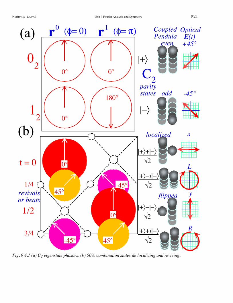
C2
0 2
1 2
r0
0°
0°
0°
180°
t = 0
1/4
1/2
3/4
0°
45°
-45°
-45°
0°
45°
-45°
|+〉
revivalsor beats
|−〉
|+〉+|−〉√2
|+〉+i|−〉√2
|+〉−i|−〉√2
|+〉−|−〉√2
(φ= 0) (φ= π)(a)
(b)
paritystates
even +45°
odd -45°
localized x
flipped y
L
R
OpticalE(t)
CoupledPendular1
Fig. 9.4.1 (a) C2 eigenstate phasors. (b) 50% combination states de localizing and reviving.
HarterSoft –LearnIt Unit 3 Fourier Analysis and Symmetry 9-21
22
At τ1/2, the left 12 clock is at 6 PM the right one at 12 PM, but both 02 clocks still read 12PM . On the left: 12 PM plus 6 PM is zero (a node). On the right: 12 PM plus 12PM is big 12 PM. All the wave flips to the |y〉-state. The 1/2-period situation is like 1/2-wave plate changing |x〉-polarization to |y〉. Still later at (3τ1/4) the initial |x〉-state has become a right circular state. (Fig. 9.4.1b bottom) |R〉 = ( |+〉 + i |−〉 )/√2 = ( |02〉 + i |12〉 )/√2 (Time t=(3/4) τ1 )Finally, at full-time (1/1)τ1 the initial |x〉 state (top of Fig. 9.4.1b) is once again back to being |x〉 and would reappear beneath Fig. 9.4.1b to begin repeating the revival sequence.
In Fig. 9.4.1b, dotted lines making an X are drawn around the phasors to connect places where wave amplitude is low like the X-pattern in Fig. 9.3.5c. Low m-uncertainty (Δm=1.5) means the revival wave is mostly a combination of the first two Bohr eigenlevels m=0 and |m|=1 having just two group (or phase) velocities +V1 and -V1. In other words, Fig. 9.3.5c is essentially just a two-state system, and the major half and full revivals are just binary beat of two coupled symmetric pendulums. The 1/4 fractional revival corresponds to transition state |L〉 = ( |x〉 − i |y〉 )/√2 (analogous to left circular polarization) between the major revivals. In |L〉 the left hand position phasor is 90° ahead of the right hand one being resonantly pumped up. The roles of the two phasors are reversed at 3τ1/4.
(b) Cn group structure: n=3, 4,...6 Eigenstates To understand finer X-zero patterns and fractional revivals between zeros in Fig. 9.3.5 a-b we go beyond the binary {|02〉 |12〉} basis to, at least, the base-3 basis {|03〉 |13〉 |23〉} of C3 The bra state vectors {〈03 | 〈13 | 〈23 |} were defined in Fig. 2.6.4 and are re-drawn in Fig. 9.4.2a. The C3 wave states have quantized momentum m=0, 1, and 2 modulo 3 . Each m labels a row of three phasors in Fig. 9.4.2a which are a discrete sampling of the waves in the first three Bohr levels m=0,1, and 2. In Fig. 9.4.2b are 4-nary C4 base states of m=0, 1, 2 and 3 modulo 4 quanta and Fig. 9.4.3a reintroduces 5-nary C5 bases of m=0, 1, 2,3, and 4 modulo 5 quanta, and similarly in Fig. 9.4.3b for C6. These systems are like counters; a binary C2 system can count only to two, that is, 0 to 1, but each of the CN systems are capable of counting to N, that is, 0, 1, 2,3,..,N-1. Physically the CN waves are bases of a finite and discrete Fourier analysis. Each CN character table in Fig. 9.4.2a-b or 9.4.3a-b (if all divided by √N) is the N-by-N unitary (U(n)) transformation matrix 〈p|m〉 of discrete Fourier transformation coefficients. (Recall Fig. 7.3.3 and discussion.)
p m( )N= ei p m/ 2πN / N = m( )N
p*
(p,m = 0,1,2,...,N - 1) (9.4.3a)
Each phasor in Fig. 9.4.2-12 sits at one of N equally spaced lattice points p=0, 1, ...,N-1. Each phasor gives for a particular angular point p=0, 1, 2,3,..,N-1 the complex wave amplitude (7.3.10a) ψ±m(2πp/N) = 〈p|(m)N 〉 = 〈(m)N |p〉* of a continuous running wave that is one of Bohr-Schrodinger eigenfunctions ψ±m(φ). A real (cosine) part of the eigenfunction is drawn for each eigenstate |(m)N〉 in Fig. 9.4.2-3 to help connect it to the latter. The state notation (m)N labels these waves and should be read m-modulo-N (or m%N in C) meaning
©2013 W. G. Harter Chapter 9 Time Evolution 9-
that waves having m± nN wavelengths or quanta will give a physically and mathematically identical state (m)N . (They are Fourier aliases (m)N = (m± nN)N, states differing only by reciprocal lattice vectors K= ± nN .) In Fig. 9.4.2-12 each one of N equally spaced lattice points p=0, 1, 2, 3,...,N-1, is labeled by a p-th power rp of a fundamental CN group rotation r by angle 2π/N , that is, by r0=1 , r1, r2, r3 ... , rN-1 , rN=1 respectively. This labeling notation simply lists the operator elements of the cyclic CN symmetry group as was done in equations (8.1.5a). The entries e-ipm/2πN are m-th eigenvalues of r0,r1,r2...,rp. The phasors are graphical representations of the complex eigenvalues or characters of the various cyclic groups. It should be noted that the binary C2 phasor table (Fig. 9.4.1a) is embedded as a subset in the C4 table since C2 is a subgroup of C4. C2 is also seen in the C6 table (Fig. 9.4.3b) or any CN table of even-N since C2 is a subgroup of all C2n. The C6 table also has the C3 table (Fig. 9.4.2a) embedded. Symmetry embedding is of utmost importance for analyzing group algebra, their representations, and their physical applications. Here it is what gives the revival structure down to the finest observable details of revival wave phase or amplitude shown in Fig. 9.3.5 a.
The same numbers (without the √N ) serve triple or quadruple duty in algebraic group theory. Besides Fourier transforms they are irreducible representations Dm(rp) of CN
D
m( )N r p( ) = e−i p m
2πN (9.4.3b)
such that Dm(a) Dm(b) = Dm(ab) .This goes along with the Dm(c) being eigenvalues of the group operators c=rp. (Note (rp)† =r -p.)
r p m( )N
= Dm( )N r p( ) m( )N
= e−i p m
2πN m( )N (9.4.3c)
m( )Nr p = D
m( )N r p( ) m( )N= e
−i p m2πN m( )N
(9.4.3d)
Also, each row of the character table in Fig. 9.4.2-3 is an eigen-bra-vector wavefunction of discrete points p or powers of rp. As shown in Sec. 9.2, each bra 〈(m)N| and ket |(m)N〉 must also be an eigenvector of any Hamiltonian operator H that commutes with CN , i.e., has CN symmetry (Hrp=rpH). So the character tables serve finally as universal energy eigenvectors and eigenstates, too. All the above apply to the generic CN groups and all their embedded subgroups which include all smaller Cn for which n is an integral divisor of N.
HarterSoft –LearnIt Unit 3 Fourier Analysis and Symmetry 9-23
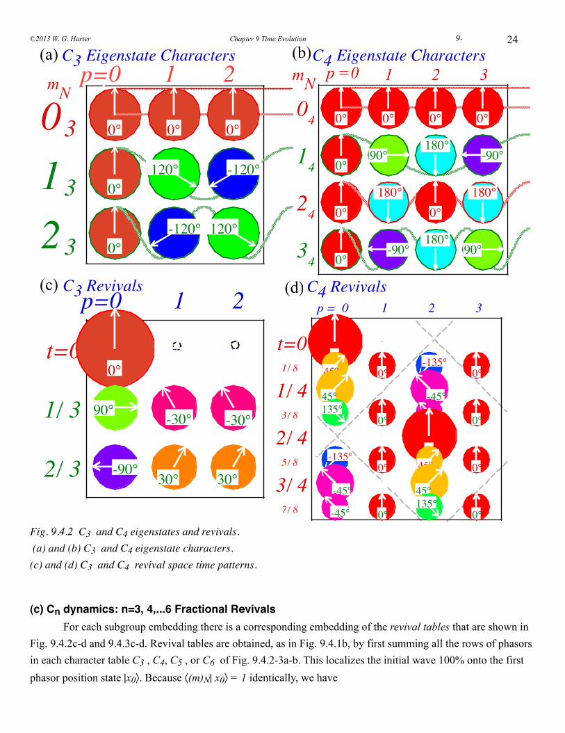
24
mN
C3 Eigenstate Characters
C3 Revivals
0 3
1 3
2 3
0°
0°
0°
0°
120°
-120°
0°
-120°
120°
t=0
1/ 3
2/ 3
p=0
0°
90°
-90°
1
-30°
30°
2
-30°
30°
p=0 1 2(a)
(c)
(b)C4 Eigenstate Charactersp =0 1 2 3mN
C4 Revivals(d)
t=0 1/ 8
1/ 4 3/ 8
2/ 4 5/ 8
3/ 4 7/ 8
p = 0
0°45°
45° 135°
-135°
-45°
-45°
1
0°
0°
0°
0°
2
-135°
-45°
-45°
0°45°
45° 135°
3
0°
0°
0°
0°
0 4
1 4
2 4
3 4
0°
0°
0°
0°
0°
90°
180°
-90°
0°
180°
0°
180°
0°
-90°
180°
90°
Fig. 9.4.2 C3 and C4 eigenstates and revivals. (a) and (b) C3 and C4 eigenstate characters. (c) and (d) C3 and C4 revival space time patterns.
(c) Cn dynamics: n=3, 4,...6 Fractional Revivals For each subgroup embedding there is a corresponding embedding of the revival tables that are shown in Fig. 9.4.2c-d and 9.4.3c-d. Revival tables are obtained, as in Fig. 9.4.1b, by first summing all the rows of phasors in each character table C3 , C4, C5 , or C6 of Fig. 9.4.2-3a-b. This localizes the initial wave 100% onto the first phasor position state |x0〉. Because 〈(m)N| x0〉 = 1 identically, we have
©2013 W. G. Harter Chapter 9 Time Evolution 9-
x0 = m( )Nm=0
N −1∑ m( )N
x0 = m( )Nm=0
N −1∑ (9.4.4a)
This is called a group completeness relation or resolution of the identity. All phasors are equivalent due to CN symmetry, so arbitrarily picking the first column (r0=1) does not affect the general utility of Fig. 9.4.2-3. Translation by rp rephases the sum (9.4.4a) according to (9.4.3c) and translates all waves rigidly.
xp = r p x0 = r p m( )Nm=0
N −1∑ = e
−ipm
2πN m( )Nm=0
N −1∑ (9.4.4b)
Then each term |(m)N〉 in the sum (9.4.3) is allowed to advance its Bohr phase e-iωmt = e-im2ω1t in discrete time fractions 1/N of τ1 for N-odd or 1/2N for N-even, that is, through stroboscopic instants tυ.
x0 (tυ ) = e−im2ω1tυ m( )N
m=0
N −1∑ tυ =
υτ1N
= 2π υω1N
υ = 1,2,..., N −1( ) for N − odd
υτ12N
= π υω1N
υ = 1,2,..., 2N −1( ) for N − even
⎧
⎨
⎪⎪
⎩
⎪⎪
(9.4.5)
For each stroboscopic instant or row in Fig. 9.4.3 there is an array of equally-sized and equally-spaced phasors, that is, a kaleidoscopic phasor array. At each tυ, phasors are either revived or else zeroed-out. An even-N=2p revival table, such as N=4 and N=6 in Fig. Fig. 9.4.3 has embedded the N=2 revival or "beat" table in Fig. Fig. 9.4.1b since C2 is a C2p subgroup. So besides the obvious 1/2-time revival halfway around, there must be 1/4-time and 3/4-time revivals for N=2 at each of the 1/4-lattice points, that is for N=6, at t=3/12 and t=9/12, and for N=4, at t=2/8 and t=6/8. Because N=6 is also divisible by 3 there will be N=3 revivals embedded at t=4/12=1/3 and t=8/12=2/3. Also, N=3 revivals embedded relative to the 1/2-time revival at t=1/3-1/2=-1/6 and t=1/3+1/2=5/6 and t=2/3-1/2=1/6 and at t=2/3+1/2=7/6. The phase angle "combinations" for each of the embedded phasors are reproduced perfectly and periodically as in a kind of quantum "odometer" or counter. An even-N revival table must start all over again at half-time, but from a point half-way around the ring at φ=π if it started at φ=0. This is required by CN symmetry and by C2 half-time revival having 100% probability on the antipodal (half-way) point p=N/2 if 100% probability starts on the initial p=0 point. So the C4 phasors below the (p=2, t=2/4=1/2) point in Fig. Fig. 9.4.3b, namely, t=5/8, 3/4, and 7/8, must have positions, amplitudes, and phases relative to the mid-point p=2 that are identical to ones at t=1/8, 1/4, and 3/8, respectively, below the initial t=0=p point. Similar repetition is seen for N=6 in Fig. 9.4.3c and for any even-N revival table below t=1/2. A prime-N revival table (like N=3 in Fig. 9.4.2c or N=5 in Fig. 9.4.3c) has no embedded structure because prime CN has no subgroup but C1. After the initial localized state each revival has probability distributed equally on all N lattice sites but with distinct phase combinations as in a kind of base-N quantum odometer. In contrast, base-N counters with N=2p , p! or other composite numbers like N=4 or 6 in Fig. 9.4.2d or 9.4.3d have the greatest variety of revival amplitudes.
HarterSoft –LearnIt Unit 3 Fourier Analysis and Symmetry 9-25
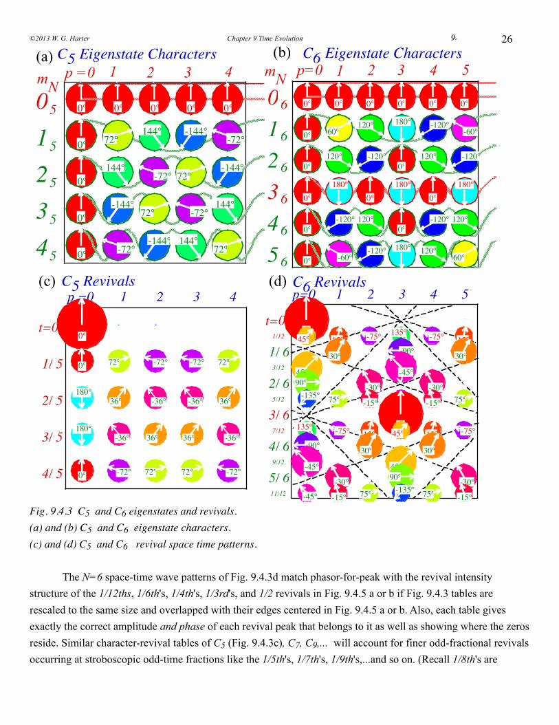
26
0 5
1 5
2 5
3 5
4 5
0°
0°
0°
0°
0°
0°
72°
144°
-144°
-72°
0°
144°
-72°
72°
-144°
0°
-144°
72°
-72°
144°
0°
-72°
-144°
144°
72°
C5 Eigenstate Charactersp =0 1 2 3 4
C5 Revivals
t=0
1/ 5
2/ 5
3/ 5
4/ 5
p =0
0°
0°
180°
180°
0°
1
72°
36°
-36°
-72°
2
-72°
-36°
36°
72°
3
-72°
-36°
36°
72°
4
72°
36°
-36°
-72°
mN
(a)
(c)
0 6
1 6
2 6
3 6
4 6
5 6
0°
0°
0°
0°
0°
0°
0°
60°
120°
180°
-120°
-60°
0°
120°
-120°
0°
120°
-120°
0°
180°
0°
180°
0°
180°
0°
-120°
120°
0°
-120°
120°
0°
-60°
-120°
180°
120°
60°
(b) C6 Eigenstate Charactersp=0 1 2 3mN 4 5
t=0 1/12
1/ 6 3/12
2/ 6 5/12
3/ 6 7/12
4/ 6 9/12
5/ 611/12
p=0
0°45°
45°90°
-135°
135°
-90°
-45°
-45°
1
15°
30°
75°
-75°
-30°
-15°
2
-75°
-30°
-15°
15°
30°
75°
3
135°
-90°
-45°
-45°
0°45°
45°90°
-135°
4
-75°
-30°
-15°
15°
30°
75°
5
15°
30°
75°
-75°
-30°
-15°
C6 Revivals(d)
Fig. 9.4.3 C5 and C6 eigenstates and revivals. (a) and (b) C5 and C6 eigenstate characters. (c) and (d) C5 and C6 revival space time patterns.
The N=6 space-time wave patterns of Fig. 9.4.3d match phasor-for-peak with the revival intensity structure of the 1/12ths, 1/6th's, 1/4th's, 1/3rd's, and 1/2 revivals in Fig. 9.4.5 a or b if Fig. 9.4.3 tables are rescaled to the same size and overlapped with their edges centered in Fig. 9.4.5 a or b. Also, each table gives exactly the correct amplitude and phase of each revival peak that belongs to it as well as showing where the zeros reside. Similar character-revival tables of C5 (Fig. 9.4.3c), C7, C9,... will account for finer odd-fractional revivals occurring at stroboscopic odd-time fractions like the 1/5th's, 1/7th's, 1/9th's,...and so on. (Recall 1/8th's are
©2013 W. G. Harter Chapter 9 Time Evolution 9-
revivals for C4 shown in Fig. 9.4.2d. They will be copied by a C8 revival table in between its (new) 1/16th's.) The medium resolution wave plot of Fig. 9.4.5b displays N=2, 3, 4, ...,8 structure more clearly than high-Δm Fig. 9.4.5a by suppressing or defocusing the even finer revivals and prolonging fewer but more robust peaks or zeros of the more fundamental revivals. But, all zero-centered excitations ( m =0) for larger-Δm such as shown in Fig. 9.4.5a-b have the same fundamental X of a (0↔1) C2 beat in Fig. 9.4.5c, that is, they show a half-time revival that peaks around the center of the largest X.
Cyclic subgroup hierarchies
Cn ⊂ Cpn ⊂ C
p2n⊂ C
p3n⊂
are here being used to organize quantum fractal revival dynamics. Schrodinger's approach to quantum theory, which eschewed the gruppenpest in favor of differential equations, is not set up to explain the origins of such discrete fractal structure. This is because each successive integer N starts a new hierarchical group family. If the integer is prime the family is entirely new. But, if it is not prime, then older smaller families belonging to each of N's factors are copied and embedded in the new family. In contrast, Schrodinger's wave equation treats every value of its independent variables as just another dumb x or t, and rational structure is glossed over.
Each new odd integer N=2m+1 will have N new revival peaks at time fractions t/τ=ν/N=1/N,...q/N .. but only for fractions q/N that are irreducible. Reducible fractions q/N that reduce to q/N = qR/r (by dividing out a highest common factor f=N/r=q/qR ) just recreate the "old" r=N/f-peak revivals already seen for a lesser or reduced integer NR =r=N/f. Similarly, for even N=2m the only new revivals are at found irreducible time
fractions t/τ=ν/2N=1/2N,...q/2N ... . All the rest belong to subgroups CNR (if any) of CN including Cm and C2. A formula for new revival phasors based on sum (9.4.5) is given in Appendix 3.A. Now we consider a quasi-classical way to understand revival dynamics. Odd-N revivals clearly display the prime factors and their multiples of the integer N. If N is a prime number as it is for N=3 in Fig. 9.4.2c and for N=5 in Fig. 9.4.3c then all reviving kaleidoscopes except the initial one consist of uniform distributions of N phasors of probability 1/N. However, for a composite odd integer such as N=15, the phasor distributions are not uniform as shown in Fig. 9.4.4. There are nodes at the p=±1 points for all revivals that correspond to factors of the integer N=15, namely at the revivals numbered 1, 3, 6, 9, 12, and 1, 5, 10, and 15. The latter are copies of C3 revivals seen in Fig. 9.4.2c and the former are copies of C5 revivals seen in Fig. 9.4.3c. Their presence is simply a result of C3 and C5 being subgroups of C15. By definition, 1 is a factor of all N and C1 is a subgroup of all CN . This is manifest by the first row of each revival table. The only even prime integer is N=2. This helps to account for the unique status of the C2 revival table in Fig. 9.4.1b and the extra significance of the C2 parity of each integer N, that is, the distinction between odd and even integers.
HarterSoft –LearnIt Unit 3 Fourier Analysis and Symmetry 9-27
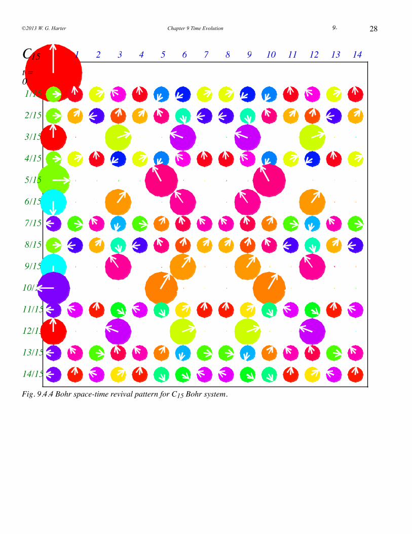
28
1
2/15
3/15
4/15
5
6/15
7/15
8/15
9/15
10/15
11/15
12/15
13/15
14/15
p =0
1 2 3 4 5 6 7 8 9 10 11 12 13 14C15t =0
/15
/15
Fig. 9.4.4 Bohr space-time revival pattern for C15 Bohr system.
©2013 W. G. Harter Chapter 9 Time Evolution 9-
Bohr vs. Bloch dispersion The value of the CN models increases when the purely quantum effects, particularly those of a single CN, are to be isolated. One imagines having a discrete Bohr ring like those sketched Fig. 9.4.5 composed of N atoms, quantum dots, optical fibers, or Josephson circuits homo-cyclically coupled is such a way that the usual quadratic Bohr dispersion spectrum ωm = m2ω1 is obtained with a finite number N of states per band. As a first approximation, such a ring has a Bloch dispersion spectrum ωm = (H0-2H1 cos am) where H1 is the nearest neighbor coupling amplitude. Such a Bloch spectrum only approximates a Bohr spectrum for low m-values, and so high-Δm revivals would decay eventually. However, by inserting cross-connecting coupling paths H2 , H3 , H4 , ...HN/2 , as shown in Fig. 9.4.5, it is possible to achieve any spectrum, including m2, by adjusting coefficients Hk in a Fourier series. ωm = H0-2S1 cos am-2H2 cos 2am-2H3 cos 3am...-HN/2 cos Nam/2 .A quadratic spectrum (Em=hυm2) is achieved for general N by setting Hamiltonian parameters as follows.
hυm2 = H p e
−i p m2πN
p=0
N −1∑ , where: H p = hυ
Nm2 e
i p m2πN
m{ }∑ (9.4.6)
For example, a 4-level N=6 quadratic spectrum {E0=0, E±1=12 E±2=22, E3=32.} involves six eigenstates: |(m)6〉 = |(0)6〉, |(±1)6〉, |(±2)6〉, and |(3)6〉, using the following coupling amplitudes as given in the N=6 row of Table 9.1. H0=3.16, H1=-2.0=H5*, H2= 0.67=H4*, H3=-0.5 , (9.4.7) With the adjustments in Table 9.1. of Hk coupling, pure CN revivals like those in Fig. 9.4.2-3 would repeat at frequency υ=h-1 until the coupling is turned off. Such a device would be an N-ary counter as implied before. By incorporating the N-ring as the crossection of a coaxial N-fiber cable, it would be possible for the revival evolution to occur as an N-phase wave propagated down the cable. The possibility of storing, processing, and transporting quantum or classical N-ary data for N>>2 using just one kind of basic hardware may yet warm the heart (and portfolio) of a future cyber-entrepreneur.
HarterSoft –LearnIt Unit 3 Fourier Analysis and Symmetry 9-29
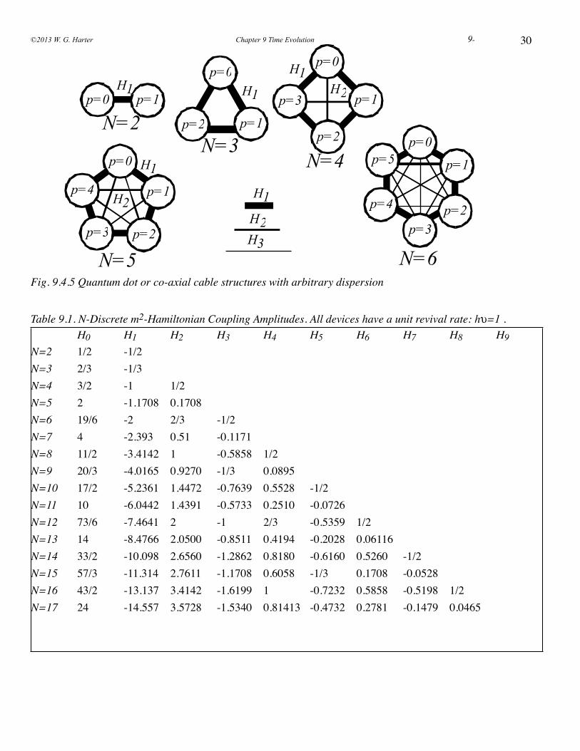
30
p=0
p=1
p=2p=3
p=4
p=5
N=6
H1H2H3
p=0
p=1
p=2p=3
p=4
N=5
H1
H2
p=1
p=0
p=2
p=3
N=4
H1H2
p=0
p=1p=2
N=3
H1p=0 p=1
N=2
H1
Fig. 9.4.5 Quantum dot or co-axial cable structures with arbitrary dispersion
Table 9.1. N-Discrete m2-Hamiltonian Coupling Amplitudes. All devices have a unit revival rate: hυ=1 .H0 H1 H2 H3 H4 H5 H6 H7 H8 H9
N=2 1/2 -1/2N=3 2/3 -1/3N=4 3/2 -1 1/2N=5 2 -1.1708 0.1708N=6 19/6 -2 2/3 -1/2N=7 4 -2.393 0.51 -0.1171N=8 11/2 -3.4142 1 -0.5858 1/2N=9 20/3 -4.0165 0.9270 -1/3 0.0895N=10 17/2 -5.2361 1.4472 -0.7639 0.5528 -1/2N=11 10 -6.0442 1.4391 -0.5733 0.2510 -0.0726N=12 73/6 -7.4641 2 -1 2/3 -0.5359 1/2N=13 14 -8.4766 2.0500 -0.8511 0.4194 -0.2028 0.06116N=14 33/2 -10.098 2.6560 -1.2862 0.8180 -0.6160 0.5260 -1/2N=15 57/3 -11.314 2.7611 -1.1708 0.6058 -1/3 0.1708 -0.0528N=16 43/2 -13.137 3.4142 -1.6199 1 -0.7232 0.5858 -0.5198 1/2N=17 24 -14.557 3.5728 -1.5340 0.81413 -0.4732 0.2781 -0.1479 0.0465
©2013 W. G. Harter Chapter 9 Time Evolution 9-
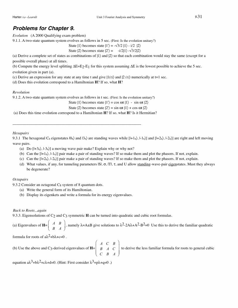
Problems for Chapter 9.Evolution (A 2000 Qualifying exam problem) 9.1.1. A two-state quantum system evolves as follows in 5 sec. (First: Is the evolution unitary?)
! ! ! State |1〉 becomes state |1'〉 = -√3/2 |1〉 - i/2 |2〉 ! ! ! State |2〉 becomes state |2'〉 = -i/2|1〉 -√3/2|2〉
(a) Derive a complete set of states as combinations of |1〉 and |2〉 so that each combination would stay the same (except for a possible overall phase) at all times. (b) Compute the energy level splitting ΔE=E2-E1 for this system assuming ΔE is the lowest possible to achieve the 5 sec. evolution given in part (a).(c) Derive an expression for any state at any time t and give |1(t)〉 and |2 (t)〉 numerically at t=1 sec.(d) Does this evolution correspond to a Hamiltonian H? If so, what H?
Revolution9.1.2. A two-state quantum system evolves as follows in t sec. (First: Is the evolution unitary?)
! ! ! State |1〉 becomes state |1'〉 = cos ωt |1〉 - sin ωt |2〉 ! ! ! State |2〉 becomes state |2'〉 = sin ωt |1〉 + cos ωt |2〉
(a) Does this time evolution correspond to a Hamiltonian H? If so, what H? Is it Hermitian?
__________________________________________________________________
Hexapairs9.3.1 The hexagonal C6 eigenstates |06〉 and |36〉 are standing waves while [|+16〉, |-16〉] and [|+26〉, |-26〉] are right and left moving wave pairs.
(a) Do [|+36〉, |-36〉] a moving wave pair make? Explain why or why not? (b) Can the [|+16〉, |-16〉] pair make a pair of standing waves? If so make them and plot the phasors. If not, explain.(c) Can the [|+26〉, |-26〉] pair make a pair of standing waves? If so make them and plot the phasors. If not, explain.(d) What values, if any, for tunneling parameters |S|, σ, |T|, τ, and U allow standing-wave-pair eigenstates. Must they always
be degenerate?
Octapairs9.3.2 Consider an octagonal C8 system of 8 quantum dots.
(a) Write the general form of its Hamiltonian.(b) Display its eigenkets and write a formula for its energy eigenvalues.
Back to Roots...again9.3.3. Eigensolutions of C2 and C3 symmetric H can be turned into quadratic and cubic root formulas.
(a) Eigenvalues of H=
A BB A
⎛
⎝⎜⎞
⎠⎟, namely λ=A±B give solutions to λ2-2Aλ+A2-B2=0 Use this to derive the familiar quadratic
formula for roots of aλ2+bλ+c=0 .
(b) Use the above and C3-derived eigenvalues of H=
A C BB A CC B A
⎛
⎝
⎜⎜⎜
⎞
⎠
⎟⎟⎟
to derive the less familiar formula for roots to general cubic
equation aλ3+bλ2+cλ+d=0. (Hint: First consider λ3+pλ+q=0 .)
HarterSoft –LearnIt Unit 3 Fourier Analysis and Symmetry 9-31
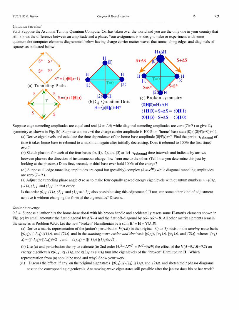
32_____________________________________________________________________________Quantum baseball9.3.3 Suppose the Asumma Tummy Quantum Computer Co. has taken over the world and you are the only one in your country that still knows the difference between an amplitude and a phase. Your assignment is to design, make or experiment with some quantum dot computer elements diagrammed below having charge carrier matter-waves that tunnel along edges and diagonals of squares as indicated below.
!
H
S
S*
TH = 〈ρ|H |ρ〉=H*
(b)C4 Quantum Dots
S S
S
S* S*
S*
H
H
H
(a) Tunneling P aths
〈0 |H|0〉=H+ΔH(c) Broken symmetry
H
H
H
H+ΔH
S+ΔS S+ΔS
〈1|H |0〉 = S+ΔS = 〈0|H|1〉
S=S* S=S*T=0
〈0|H |3〉 = S+ΔS = 〈3|H|0〉
|0〉
|2〉
|3〉|1〉
|2〉
|3〉
|0〉
|1〉
S = 〈ρ+1|H|ρ〉
S* = 〈ρ|H|ρ+1〉T=0
Suppose edge tunneling amplitudes are equal and real (S =-1.0) while diagonal tunneling amplitudes are zero (T=0 ) to give C4 symmetry as shown in Fig. (b). Suppose at time t=0 the charge carrier amplitude is 100% on "home" base state |0〉.( 〈0|Ψ(t=0)〉=1).
(a) Derive eigenlevels and calculate the time dependence of the home-base amplitude 〈0|Ψ(t)〉=? Find the period τrebound of time it takes home-base to rebound to a maximum again after initially decreasing. Does it rebound to 100% the first time? ever? (b) Sketch phasors for each of the four bases |0〉, |1〉, |2〉, and |3〉 at 1/4- τrebound time intervals and indicate by arrows between phasors the direction of instantaneous charge flow from one to the other. (Tell how you determine this just by looking at the phasors.) Does first, second, or third base ever hold 100% of the charge?(c.) Suppose all edge tunneling amplitudes are equal but (possibly) complex (S =-eiσ) while diagonal tunneling amplitudes are zero (T=0 ). (a) Adjust the tunneling phase angle σ so as to make four equally spaced energy eigenlevels with quantum numbers m=(0)4, (-1)4, (1)4, and (2)4 , in that order. Is the order (0)4, (1)4, (2)4, and (3)4 = (-1)4 also possible using this adjustment? If not, can some other kind of adjustment achieve it without changing the form of the eigenstates? Discuss.
Janitor’s revenge9.3.4. Suppose a janitor hits the home-base dot-0 with his broom handle and accidentally resets some H-matrix elements shown in Fig. (c) by small amounts: the first diagonal by ΔH=A and the first off-diagonal by ΔS=ΔS*=B. All other matrix elements remain the same as in Problem 9.3.3. Let the new "broken" Hamiltonian be a sum H' = H + V(A,B).
(a) Derive a matrix representation of the janitor's perturbation V(A,B) in the original |0〉 to |3〉 basis, in the moving-wave basis |(0)4〉, |(-1)4〉, |(1)4〉, and |(2)4〉, and in the standing-wave cosine and sine basis |(0)4〉, |(c1)4〉, |(s1)4〉, and |(2)4〉, where: !|(c1)
4〉 = (|(-1)4〉+|(1)4〉)/√2 , and: |(s1)4〉 = (|(-1)4〉-|(1)4〉)/i√2 .
(b) Use (a) and perturbation theory to estimate (to 2nd order |A|2=|ΔS|2 or |b|2=|ΔH|) the effect of the V(A=0.1,B=0.2) on energy eigenlevels ε(0)4, ε(±1)4, and ε(2)4 as ε(m)4 turn into eigenlevels of the "broken" Hamiltonian H'. Which representation from (a) should be used and why? Show your work.
(c.) Discuss the effect, if any, on the original eigenstates |(0)4〉, |(-1)4〉, |(1)4〉, and |(2)4〉, and sketch their phasor diagrams next to the corresponding eigenlevels. Are moving-wave eigenstates still possible after the janitor does his or her work?
©2013 W. G. Harter Chapter 9 Time Evolution 9-
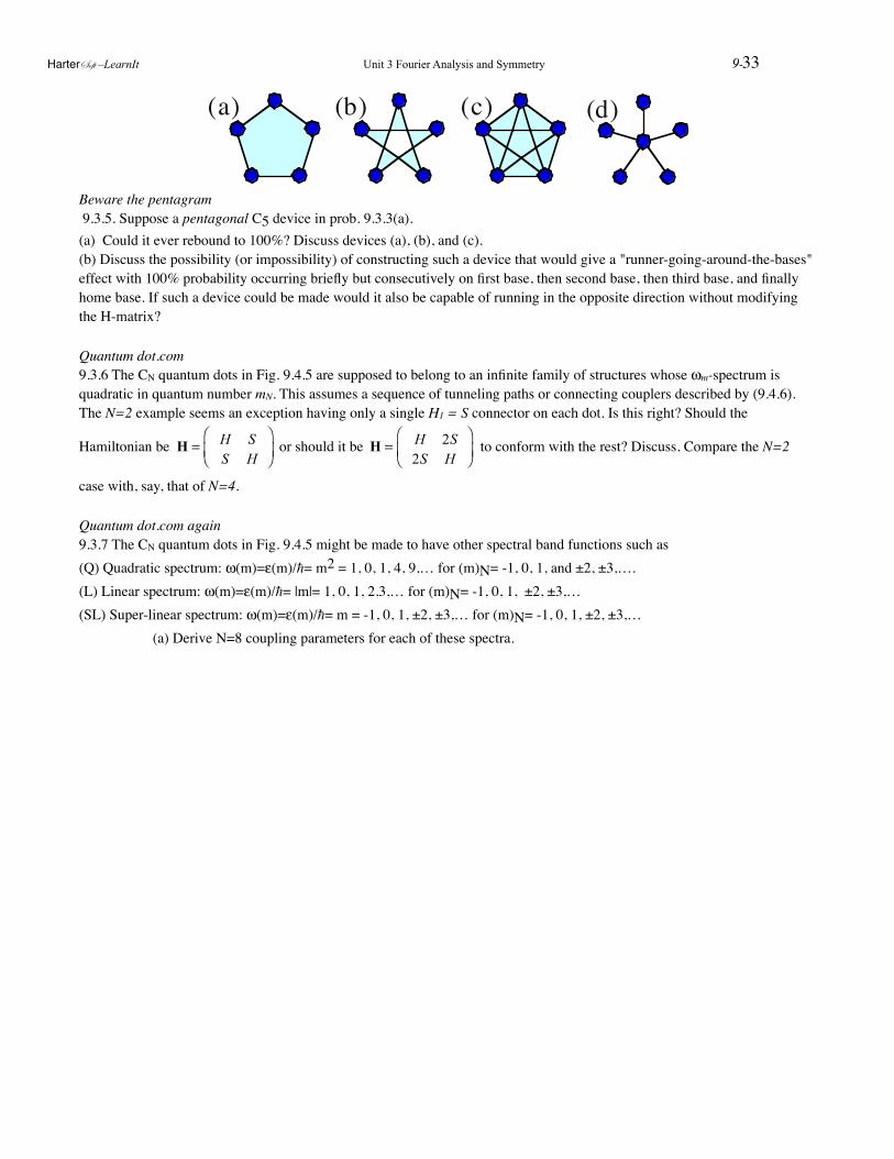
! !
(a) (b) (c) (d)
Beware the pentagram 9.3.5. Suppose a pentagonal C5 device in prob. 9.3.3(a). (a) Could it ever rebound to 100%? Discuss devices (a), (b), and (c).(b) Discuss the possibility (or impossibility) of constructing such a device that would give a "runner-going-around-the-bases" effect with 100% probability occurring briefly but consecutively on first base, then second base, then third base, and finally home base. If such a device could be made would it also be capable of running in the opposite direction without modifying the H-matrix?
Quantum dot.com9.3.6 The CN quantum dots in Fig. 9.4.5 are supposed to belong to an infinite family of structures whose ωm-spectrum is quadratic in quantum number mN. This assumes a sequence of tunneling paths or connecting couplers described by (9.4.6).The N=2 example seems an exception having only a single H1 = S connector on each dot. Is this right? Should the
Hamiltonian be H = H S
S H
⎛
⎝⎜⎞
⎠⎟ or should it be
H = H 2S
2S H
⎛
⎝⎜⎞
⎠⎟ to conform with the rest? Discuss. Compare the N=2
case with, say, that of N=4.
Quantum dot.com again9.3.7 The CN quantum dots in Fig. 9.4.5 might be made to have other spectral band functions such as (Q) Quadratic spectrum: ω(m)=ε(m)/= m2 = 1, 0, 1, 4, 9,… for (m)N= -1, 0, 1, and ±2, ±3,….(L) Linear spectrum: ω(m)=ε(m)/= |m|= 1, 0, 1, 2,3,… for (m)N= -1, 0, 1, ±2, ±3,…(SL) Super-linear spectrum: ω(m)=ε(m)/= m = -1, 0, 1, ±2, ±3,… for (m)N= -1, 0, 1, ±2, ±3,…! (a) Derive N=8 coupling parameters for each of these spectra.
HarterSoft –LearnIt Unit 3 Fourier Analysis and Symmetry 9-33
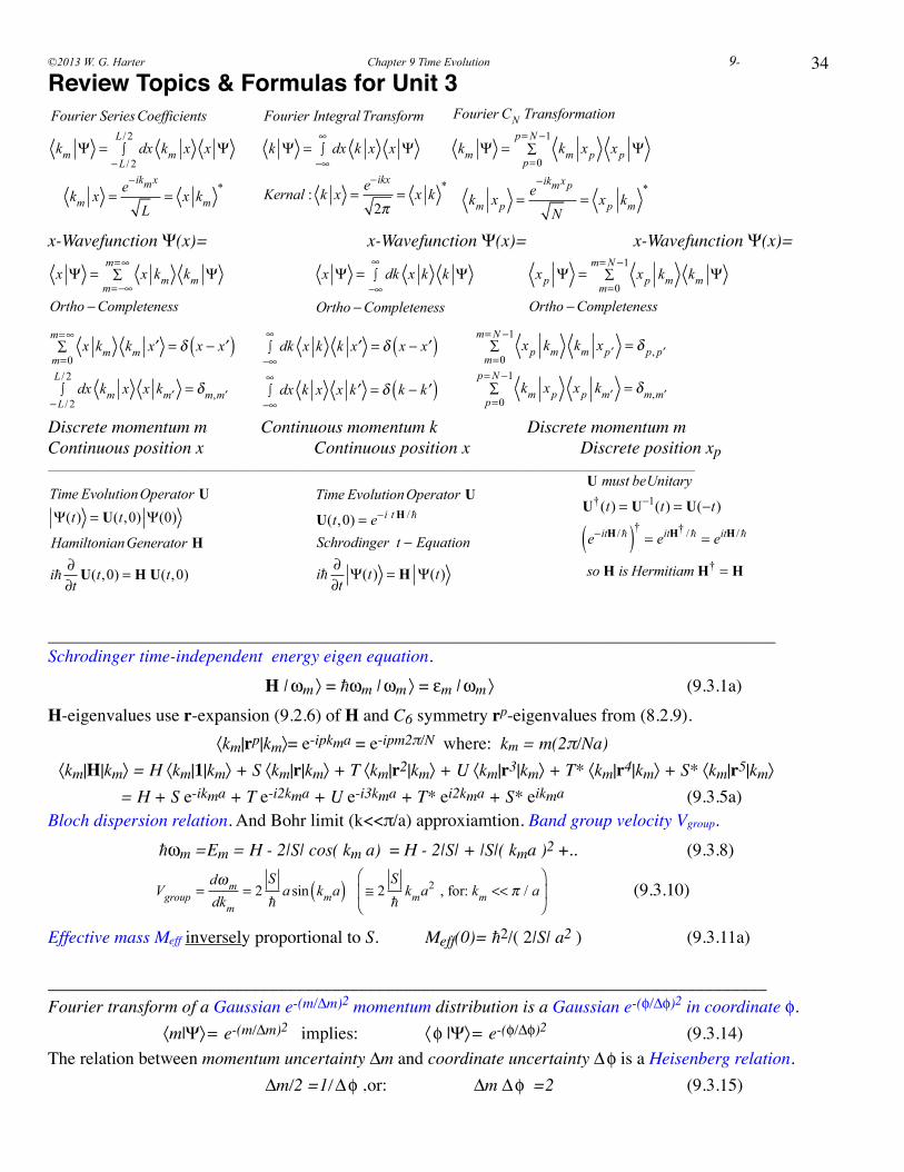
34Review Topics & Formulas for Unit 3
Fourier SeriesCoefficients
km Ψ = dx−L / 2
L / 2∫ km x x Ψ
km x = e−ikmx
L= x km
*
!
Fourier Integral Transform
k Ψ = dx−∞
∞∫ k x x Ψ
Kernal : k x = e−ikx
2π= x k
*
Fourier CN Transformation
km Ψ = km xp xp Ψp=0
p=N −1∑
km xp = e−ikmxp
N= xp km
*
x-Wavefunction Ψ(x)=! ! ! x-Wavefunction Ψ(x)=! ! x-Wavefunction Ψ(x)=
x Ψ = x km km Ψm=−∞
m=∞∑
Ortho −Completeness! !
x Ψ = dk−∞
∞∫ x k k Ψ
Ortho −Completeness!
xp Ψ = xp km km Ψm=0
m=N −1∑
Ortho −Completeness
x km km ′xm=0
m=∞∑ = δ x − ′x( )
dx−L / 2
L / 2∫ km x x k ′m = δm, ′m
!
dk−∞
∞∫ x k k ′x = δ x − ′x( )
dx−∞
∞∫ k x x ′k = δ k − ′k( )
!
xp km km x ′pm=0
m=N −1∑ = δ p, ′p
km xp xp k ′mp=0
p=N −1∑ = δm, ′m
Discrete momentum m!! Continuous momentum k! ! Discrete momentum mContinuous position x!! ! Continuous position x!! ! Discrete position xp_____________________________________________________________________________________________________________________________
Time EvolutionOperator UΨ(t) = U(t,0) Ψ(0)
HamiltonianGenerator H
i ∂∂t
U(t,0) = H U(t,0)
! !
Time EvolutionOperator U
U(t,0) = e−i t H /
Schrodinger t − Equation
i ∂∂t
Ψ(t) = H Ψ(t)
! !
U must beUnitary
U†(t) = U−1(t) = U(−t)
e−itH /( )† = eitH† / = eitH /
so H is Hermitiam H† = H
__________________________________________________________________________________Schrodinger time-independent energy eigen equation.! ! ! ! H | ωm 〉 = ωm | ωm 〉 = εm | ωm 〉! ! ! ! (9.3.1a)H-eigenvalues use r-expansion (9.2.6) of H and C6 symmetry rp-eigenvalues from (8.2.9).! ! ! 〈km|rp|km〉= e-ipkma = e-ipm2π/N where: km = m(2π/Na) 〈km|H|km〉 = H 〈km|1|km〉 + S 〈km|r|km〉 + T 〈km|r2|km〉 + U 〈km|r3|km〉 + T* 〈km|r4|km〉 + S* 〈km|r5|km〉6 = H + S e-ikma + T e-i2kma + U e-i3kma + T* ei2kma + S* eikma! ! ! (9.3.5a) Bloch dispersion relation. And Bohr limit (k<<π/a) approxiamtion. Band group velocity Vgroup.! ! ωm =Em = H - 2|S| cos( km a) = H - 2|S| + |S|( kma )2 +..! ! ! (9.3.8)
! !
Vgroup =dωmdkm
= 2S
a sin kma( ) ≅ 2
S
kma2 , for: km << π / a
⎛
⎝⎜
⎞
⎠⎟ ! ! (9.3.10)
Effective mass Meff inversely proportional to S.! Meff(0)= 2/( 2|S| a2 )! ! (9.3.11a)
_________________________________________________________________________________Fourier transform of a Gaussian e-(m/Δm)2 momentum distribution is a Gaussian e-(φ/Δφ)2 in coordinate φ. ! ! 〈m|Ψ〉 = e-(m/Δm)2 implies:! ! 〈 φ |Ψ〉 = e-(φ/Δφ)2 ! ! ! (9.3.14)The relation between momentum uncertainty Δm and coordinate uncertainty Δ φ is a Heisenberg relation.! ! ! ! Δm/2 =1/ Δ φ ,!or: ! ! Δm Δ φ =2 ! ! ! (9.3.15)
©2013 W. G. Harter Chapter 9 Time Evolution 9-
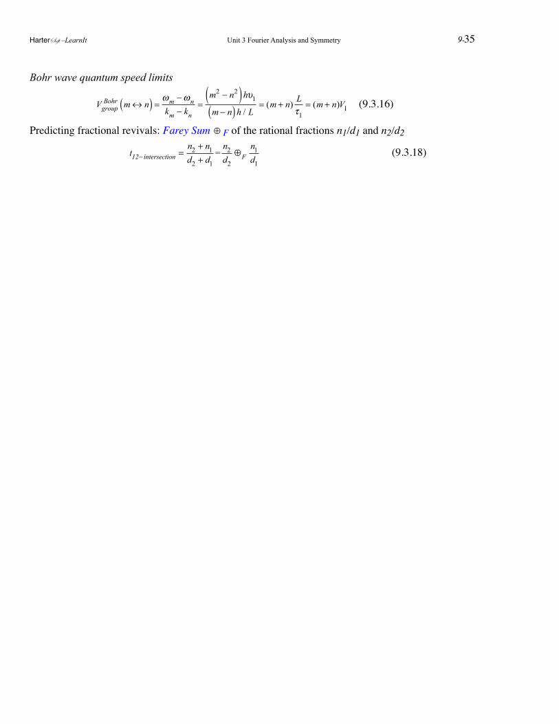
Bohr wave quantum speed limits
! ! Vgroup
Bohr m ↔ n( ) = ωm −ωnkm − kn
=m2 − n2( )hυ1
m − n( )h / L= (m + n) L
τ1= (m + n)V1 ! (9.3.16)
Predicting fractional revivals: Farey Sum ⊕ F of the rational fractions n1/d1 and n2/d2
! ! ! t12− intersection =
n2 + n1d2 + d1
=n2d2
⊕Fn1d1! ! ! ! (9.3.18)
HarterSoft –LearnIt Unit 3 Fourier Analysis and Symmetry 9-35
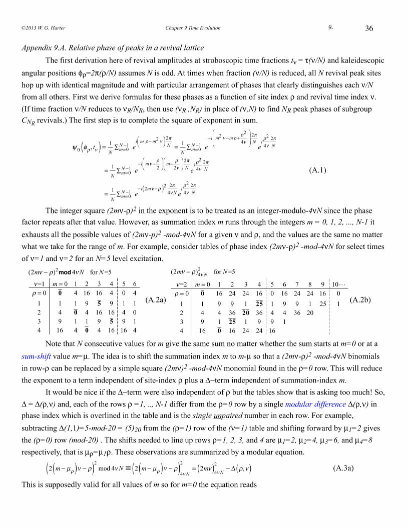
36
Appendix 9.A. Relative phase of peaks in a revival lattice The first derivation here of revival amplitudes at stroboscopic time fractions tν = τ(ν/N) and kaleidescopic angular positions φρ=2π(ρ/N) assumes N is odd. At times when fraction (ν/N) is reduced, all N revival peak sites hop up with identical magnitude and with particular arrangement of phases that clearly distinguishes each ν/N from all others. First we derive formulas for these phases as a function of site index ρ and revival time index ν. (If time fraction ν/N reduces to νR/NR, then use (νR ,NR) in place of (ν,N) to find NR peak phases of subgroup CNR revivals.) The first step is to complete the square of exponent in sum.
ψ 0 φρ , tν( ) = 1
N m=0N −1∑ e
i m ρ− m2 ν⎛⎝⎜
⎞⎠⎟
2πN = 1
N m=0N −1∑ e
−i m2 ν−mρ+ ρ2
4ν
⎛
⎝⎜⎜
⎞
⎠⎟⎟
2πN
ei ρ
2
4ν2πN
= 1
N m=0N −1∑ e
−i mν− ρ2
⎛⎝⎜
⎞⎠⎟
m−ρ
2ν⎛⎝⎜
⎞⎠⎟
2πN e
i ρ2
4ν2πN
= 1
N m=0N −1∑ e
−i 2mν−ρ( )2 2π4νN e
i ρ2
4ν2πN
(A.1)
The integer square (2mν-ρ)2 in the exponent is to be treated as an integer-modulo-4νN since the phase factor repeats after that value. However, as summation index m runs through the integers m = 0, 1, 2, ..., N-1 it exhausts all the possible values of (2mν-p)2 -mod-4νN for a given ν and ρ, and the values are the same no matter what we take for the range of m. For example, consider tables of phase index (2mν-ρ)2 -mod-4νN for select times of ν=1 and ν=2 for an N=5 level excitation.
(2mν − ρ)2mod4νN for N =5
ν=1 m = 0 1 2 3 4 5 6ρ = 0 0 4 16 16 4 0 4
1 1 1 9 5 9 1 12 4 0 4 16 16 4 03 9 1 1 9 5 9 14 16 4 0 4 16 16 4
(A.2a)
(2mν − ρ)4νN2 for N =5
ν=2 m = 0 1 2 3 4 5 6 7 8 9 10ρ = 0 0 16 24 24 16 0 16 24 24 16 0
1 1 9 9 1 25 1 9 9 1 25 12 4 4 36 20 36 4 4 36 203 9 1 25 1 9 9 14 16 0 16 24 24 16
(A.2b)
Note that N consecutive values for m give the same sum no matter whether the sum starts at m=0 or at a sum-shift value m=µ. The idea is to shift the summation index m to m-µ so that a (2mν-ρ)2 -mod-4νN binomials in row-ρ can be replaced by a simple square (2mν)2 -mod-4νN monomial found in the ρ=0 row. This will reduce the exponent to a term independent of site-index ρ plus a Δ−term independent of summation-index m. It would be nice if the Δ−term were also independent of ρ but the tables show that is asking too much! So, Δ = Δ(ρ,ν) and, each of the rows ρ =1, .., N-1 differ from the ρ=0 row by a single modular difference Δ(ρ,ν) in phase index which is overlined in the table and is the single unpaired number in each row. For example, subtracting Δ(1,1)=5-mod-20 = (5)20 from the (ρ=1) row of the (ν=1) table and shifting forward by µ1=2 gives the (ρ=0) row (mod-20) . The shifts needed to line up rows ρ=1, 2, 3, and 4 are µ1=2, µ2=4, µ3=6, and µ4=8 respectively, that is µρ=µ1ρ. These observations are summarized by a modular equation.
2 m − µρ( )ν − ρ( )2 mod 4νN ≡ 2 m − µρ( )ν − ρ( )4νN
2= 2mν( )4νN
2− Δ ρ,ν( ) (A.3a)
This is supposedly valid for all values of m so for m=0 the equation reads
©2013 W. G. Harter Chapter 9 Time Evolution 9-
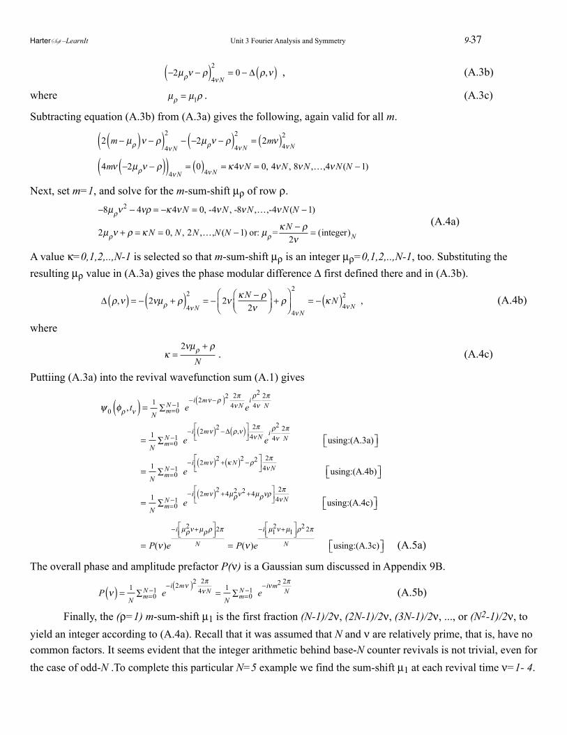
−2µρν − ρ( )
4νN
2= 0 − Δ ρ,ν( ) , (A.3b)
where µρ = µ1ρ . (A.3c)
Subtracting equation (A.3b) from (A.3a) gives the following, again valid for all m.
2 m − µρ( )ν − ρ( )4νN
2− −2µρν − ρ( )
4νN
2= 2mν( )4νN
2
4mν −2µρν − ρ( )( )4νN
= 0( )4νN= κ 4νN = 0, 4νN , 8νN ,…,4νN (N −1)
Next, set m=1, and solve for the m-sum-shift µρ of row ρ.
−8µρν2 − 4νρ = −κ 4νN = 0, -4νN , -8νN ,…,-4νN (N −1)
2µρν + ρ = κN = 0, N , 2N ,…,N (N −1) or: µρ=κN − ρ
2ν= (integer)N
(A.4a)
A value κ=0,1,2,..,N-1 is selected so that m-sum-shift µρ is an integer µρ=0,1,2,..,N-1, too. Substituting the resulting µρ value in (A.3a) gives the phase modular difference Δ first defined there and in (A.3b).
Δ ρ,ν( ) = − 2νµρ + ρ( )
4νN
2= − 2ν κN − ρ
2ν⎛⎝⎜
⎞⎠⎟+ ρ
⎛
⎝⎜⎞
⎠⎟ 4νN
2
= − κN( )4νN2
, (A.4b)
where
κ =
2νµρ + ρ
N. (A.4c)
Puttiing (A.3a) into the revival wavefunction sum (A.1) gives
ψ 0 φρ , tν( ) = 1
N m=0N −1∑ e
−i 2mν−ρ( )2 2π4νN e
i ρ2
4ν2πN
= 1
N m=0N −1∑ e
−i 2mν( )2 −Δ ρ,ν( )⎡⎣⎢
⎤⎦⎥
2π4νN e
i ρ2
4ν2πN using:(A.3a)⎡⎣ ⎤⎦
= 1
N m=0N −1∑ e
−i 2mν( )2 + κ N( )2 −ρ2⎡⎣⎢
⎤⎦⎥
2π4νN using:(A.4b)⎡⎣ ⎤⎦
= 1
N m=0N −1∑ e
−i 2mν( )2 +4µρ2ν2 +4µρνρ
⎡⎣⎢
⎤⎦⎥
2π4νN using:(A.4c)⎡⎣ ⎤⎦
= P(ν )e
−i µρ2ν+µρρ
⎡⎣⎢
⎤⎦⎥2π
N = P(ν )e
−i µ12ν+µ1
⎡⎣⎢
⎤⎦⎥ρ2 2π
N using:(A.3c)⎡⎣ ⎤⎦ (A.5a)
The overall phase and amplitude prefactor P(ν) is a Gaussian sum discussed in Appendix 9B.
P ν( ) = 1
N m=0N −1∑ e
−i 2mν( )2 2π4νN = 1
N m=0N −1∑ e
−iνm2 2πN (A.5b)
Finally, the (ρ=1) m-sum-shift µ1 is the first fraction (N-1)/2ν, (2N-1)/2ν, (3N-1)/2ν, ..., or (N2-1)/2ν, to yield an integer according to (A.4a). Recall that it was assumed that N and ν are relatively prime, that is, have no common factors. It seems evident that the integer arithmetic behind base-N counter revivals is not trivial, even for the case of odd-N .To complete this particular N=5 example we find the sum-shift µ1 at each revival time ν=1- 4.
HarterSoft –LearnIt Unit 3 Fourier Analysis and Symmetry 9-37
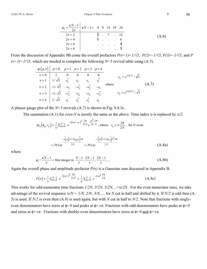
38
µ1 =κN −1
2νκN −1= 4 9 14 19 24
2ν = 2 2 . 7 . 122ν = 4 1 . . . 62ν = 6 . . . . 42ν = 8 . . . . 3
(A.6)
From the discussion of Appendix 9B come the overall prefactors P(v=1)=1/√5, P(2)=-1/√5, P(3)=-1/√5, and P(v=1)=1/√5, which are needed to complete the following N=5 revival table using (A.5).
ψ ρ,ν( ) ρ = 0 ρ = 1 ρ = 2 ρ = 3 ρ = 4
ν = 0 1 0 0 0 0ν = 1 1 / 5 e1
* e1 e1 e1*
ν = 2 −1 / 5 −e2 −e2* −e2
* −e2
ν = 3 −1 / 5 −e2* −e2 −e2 −e2
*
ν = 4 1 / 5 e1 e1* e1
* e1
where:
e1 = ei2π /5 / 5
e2 = e2i2π /5 / 5
(A.7)
A phasor gauge plot of the N=5 revivals (A.7) is shown in Fig. 9.4.3c. The summation (A.1) for even-N is mostly the same as the above. Time index υ is replaced by υ/2.
ψ 0 φρ , tν( ) = 1
N m=0N −1∑ e
−i mν−ρ( )2 2π2νN e
i ρ2
2ν2πN , where; tν = ν 2π
2N, for N -even.
= P(ν )e
−i µρ2ν+2µρρ
⎡⎣⎢
⎤⎦⎥2π
2N = P(ν )e
−i µ12ν+2µ1
⎡⎣⎢
⎤⎦⎥ρ2 2π
2N (A.8a)
where
µ1=κN −1
ν= first integer in N −1
ν, 2N −1
ν, 3N −1
ν, ... (A.8b)
Again the overall phase and amplitude prefactor P(ν) is a Gaussian sum discussed in Appendix B.
P ν( ) = 1
N m=0N −1∑ e
−i mν( )2 2π2νN = 1
N m=0N −1∑ e
−iνm2 2π2N (A.8c)
This works for odd-numerator time fractions 1/2N, 3/2N, 5/2N,...=υ/2N . For the even numerator ones, we take advantage of the revival sequence υ/N = 1/N, 2/N, 3/N,.... for N cut in half and shifted by π. If N/2 is odd then (A.5) is used. If N/2 is even then (A.8) is used again, but with N cut in half to N/2. Note that fractions with singly-even denominators have zeros at φ=0 and peaks at φ=±π. Fractions with odd denominators have peaks at φ=0 and zeros at φ=±π. Fractions with doubly-even denominators have zeros at φ=0 and φ=±π.
©2013 W. G. Harter Chapter 9 Time Evolution 9-
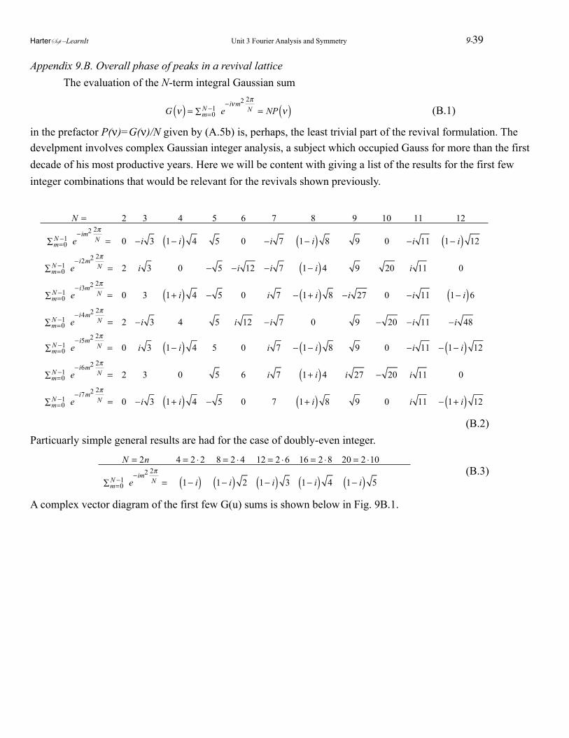
Appendix 9.B. Overall phase of peaks in a revival lattice The evaluation of the N-term integral Gaussian sum
G ν( ) = m=0
N −1∑ e−iνm2 2π
N = NP ν( ) (B.1)
in the prefactor P(ν)=G(ν)/N given by (A.5b) is, perhaps, the least trivial part of the revival formulation. The develpment involves complex Gaussian integer analysis, a subject which occupied Gauss for more than the first decade of his most productive years. Here we will be content with giving a list of the results for the first few integer combinations that would be relevant for the revivals shown previously.
N = 2 3 4 5 6 7 8 9 10 11 12
m=0N −1∑ e
−im2 2πN = 0 −i 3 1− i( ) 4 5 0 −i 7 1− i( ) 8 9 0 −i 11 1− i( ) 12
m=0N −1∑ e
−i2m2 2πN = 2 i 3 0 − 5 −i 12 −i 7 1− i( )4 9 20 i 11 0
m=0N −1∑ e
−i3m2 2πN = 0 3 1+ i( ) 4 − 5 0 i 7 − 1+ i( ) 8 −i 27 0 −i 11 1− i( )6
m=0N −1∑ e
−i4m2 2πN = 2 −i 3 4 5 i 12 −i 7 0 9 − 20 −i 11 −i 48
m=0N −1∑ e
−i5m2 2πN = 0 i 3 1− i( ) 4 5 0 i 7 − 1− i( ) 8 9 0 −i 11 − 1− i( ) 12
m=0N −1∑ e
−i6m2 2πN = 2 3 0 5 6 i 7 1+ i( )4 i 27 − 20 i 11 0
m=0N −1∑ e
−i7m2 2πN = 0 −i 3 1+ i( ) 4 − 5 0 7 1+ i( ) 8 9 0 i 11 − 1+ i( ) 12
(B.2)Particuarly simple general results are had for the case of doubly-even integer.
N = 2n 4 = 2 ⋅2 8 = 2 ⋅4 12 = 2 ⋅6 16 = 2 ⋅8 20 = 2 ⋅10
m=0N −1∑ e
−im2 2πN = 1− i( ) 1− i( ) 2 1− i( ) 3 1− i( ) 4 1− i( ) 5
(B.3)
A complex vector diagram of the first few G(u) sums is shown below in Fig. 9B.1.
!
HarterSoft –LearnIt Unit 3 Fourier Analysis and Symmetry 9-39
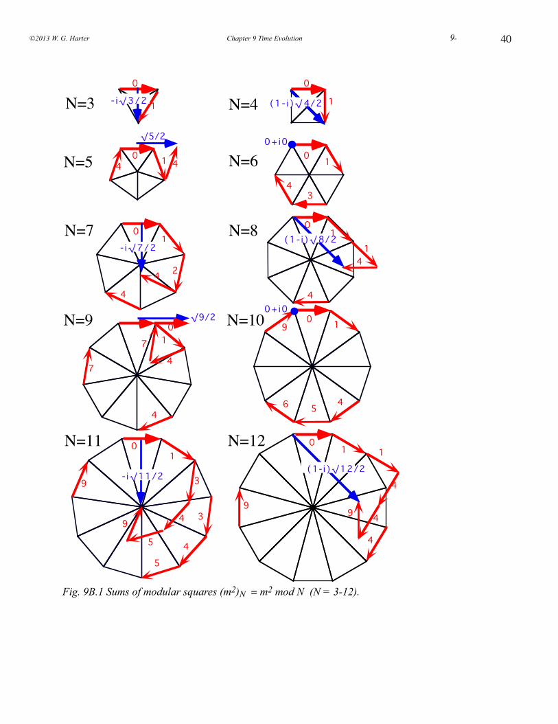
40
!
0 1
4
4
1
9
01
4
9
4
9
5
3495
3
0
1
01
0 14 40 1
43
√5/2 0+ i0
0
4
0 1
4
0+ i0
01
4
01
4
7
√9/2
24
47
14
6 5
9
N=3
N=5
N=7
N=9
N=11
N=4
N=6
N=8
N=10
N=12
(1- i )√4/2
(1- i )√8/2
(1- i )√12/2- i√11/2
- i√3/2
- i√7/21
Fig. 9B.1 Sums of modular squares (m2)N = m2 mod N (N = 3-12).
©2013 W. G. Harter Chapter 9 Time Evolution 9-

HarterSoft –LearnIt Unit 3 Fourier Analysis and Symmetry 9-41
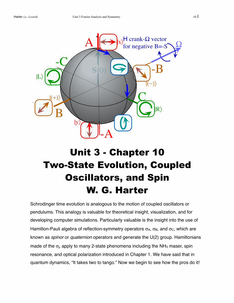
A
-A
C
-C
B
-B
H crank-Ω vectorfor negative B=-S
|(+)〉
|(−)〉
|R〉
|L〉
|x〉
|y〉
Ω
Unit 3 - Chapter 10Two-State Evolution, Coupled
Oscillators, and SpinW. G. Harter
Schrodinger time evolution is analogous to the motion of coupled oscillators or pendulums. This analogy is valuable for theoretical insight, visualization, and for developing computer simulations. Particularly valuable is the insight into the use of
Hamilton-Pauli algebra of reflection-symmetry operators σA, σB, and σC, which are
known as spinor or quaternion operators and generate the U(2) group. Hamiltonians
made of the σµ apply to many 2-state phenomena including the NH3 maser, spin
resonance, and optical polarization introduced in Chapter 1. We have said that in quantum dynamics, “It takes two to tango.” Now we begin to see how the pros do it!
HarterSoft –LearnIt Unit 3 Fourier Analysis and Symmetry 10-1

2
....................................................CHAPTER 10. TWO-STATE EVOLUTION AND ANALOGIES! 4
................................................................................................................10.1 Mechanical Analogies to Schrodinger Dynamics 4.....................................................................................................................................(a). ABCD Symmetry operator analysis 6
.........................................................................................................................................10.2 The ABCD’s of 2-State Dynamics 8..............................................................................................................................(a) Asymmetric-Diagonal or C2A symmetry 8
..................................................................................................................................................(b) Bilateral or C2B symmetry 10...................................................................................................................C2B projectors and eigenstates: Normal modes 11
............................................................................................................Understanding C2B eigenstates: Tunneling splitting 12...........................................................................................Understanding C2B dynamics: Beats and transition frequency 13
...................................................................................................................................................(c) Circular or C2C symmetry 17............................................................................................................................R(2)=C∞ projectors and C2C eigenstates 18
...................................................Understanding C2C eigenstates: Zeeman-like splitting and coriolis or cyclotron motion 19..................................................................................................................Understanding C2C dynamics: Faraday rotation 22
....................................................................................................................................................10.3 Mixed A and B Symmetry 25................................................................................................(a) Asymmetric bilateral C2AB symmetry: Stark-like-splitting 25
....................................................................................................High field splitting: Strong C2A or weak C2B symmetry 26..............................................................Low field splitting: Strong C2B or weak C2A symmetry and A→B basis change 29
........................................................................................................................................................(b) Ammonia (NH3) maser 29.....................................................................................................................................C2AB Symmetry : Weyl reflections 31
..........................................................................................................................Unitary U(2) versus Special Unitary SU(2) 33................................................................................................................................Complete sets of commuting operators 33
..............................................................................................................10.4 Mixed ABCD Symmetry: U(2) quantum systems 34........................................................................................(a) ABC Symmetry catalog: Standing, moving, or galloping waves 35
....................................................................................A, B, and AB-Archetypes are standing waves (Linear polarization) 35.....................................................................................................C-Archetypes are moving waves (Circular polarization) 35
..................................................................................................….All others are galloping waves (Elliptical polarization) 35..............................................................................................................................................(b) General HABCD eigenvalues 36
....................................................................................................10.5 Spin-Vector Pictures for Two-State Quantum Systems 38..............................................................................................................................(a) Density operators and Pauli σ-operators 40
............................................................................................(b) Hamiltonian operators and Pauli-Jordan spin operators (J=S) 43....................................................................................................................................(c) Bloch equations and spin precession 44
.............................................................................................................................Magnetic spin precession (ESR, NMR,..) 45..................................................................................................................(d) Visualizing quantum dynamics as S-precession 46
Crank Ω polar angles (ϕ,ϑ ...............................................................................................) versus Spin S polar angles (α,β) 49........................................................................Hamilton’s generalization of exp(-iω t)=cosω t-isinω t : exp(-i σ t)=What? 51
.........................................................................................................................................................................Why the 1/2? 52
............................................................................................................................................................Problems for Chapter 10. 53
..........................................................................REVIEW TOPICS & FORMULAS FOR UNIT 3! 57......................................................................................................................U(2)-R(3) Two-State and Spin-Vector Summary 60
........................................................................................................Appendix 10.A. U(2) Angles and Spin Rotation Operators 2..............................................................................................................................(a) Equivalence transformations of rotations 5
....................................................................................................................(b) Euler equivalence transformations of 3-vectors 5...................................................................................................................(c) Euler angle goniometer: Double valued position 6
......................................................................................................................(d) Axis angle rotation: Double valued operation 11.....................................................................................................................(1) Combining rotations: U(2) group products 13
..........................................................................................................................(2) Mirror reflections and Hamilton's turns 13..............................................................................................................(3) Similarity transformation and Hamilton's turns 15
.................................................................................................................................(e) Quaternion and spinor algebra (again) 16.........................................................................................................................................Why rotations are such a big deal 17
©2013 W. G. Harter Chapter10 Two-State Time Evolution 10-

.............................................................................................................................Appendix 10.B Spin control and ellipsometry 1.........................................................................................................................(a). Polarization ellipsometry coordinate angles 6
.....................................................................................................................................(1) Type-A ellipsometry Euler angles 7
.....................................................................................................................................(2) Type-C ellipsometry Euler angles 9............................................................................................................................................(b) Beam evolution of polarization 13
............................................................................................................................................Problems for Appendix 10.A and B 14
HarterSoft –LearnIt Unit 3 Fourier Analysis and Symmetry 10-3
4Chapter 10. Two-State Evolution and Analogies10.1 Mechanical Analogies to Schrodinger Dynamics The quantum Schrodinger time evolution equations (9.2.5) are similar to the classical Newtonian equations of motion for coupled pendulums. This analogy may help to understand quantum dynamics in this and later chapters. Indeed, for certain constant H Hamiltonian operators, the classical and quantum equations are mathematically and dynamically identical. Also, the concept of spin will be introduced. We begin with the simplest non-trivial quantum systems having just two-states (N=2) such as optical polarization and electron spin-polarization introduced in Chapter 1. This U(2) system is such an experimentally important system that we will devote several units to its technology. This chapter will provide an introduction to U(2) systems and their symmetry by using classical mechanical analogies. The simplest non-trivial quantum system is the two-level atom or a spin-1/2 particle. The Schrodinger equation (9.2.5) for these systems has the general form:
i ∂
∂tΨ t( ) = H Ψ t( ) (10.1.1a)
where H is a two-by-two Hermitian (H†=H) matrix operator
H = A B − iC
B + iC D⎛
⎝⎜⎞
⎠⎟. (10.1.1b)
and ket Ψ is a two-dimensional complex phasor vector xj+ipj
Ψ =Ψ1
Ψ2
⎛
⎝⎜⎜
⎞
⎠⎟⎟=
x1 + ip1
x2 + ip2
⎛
⎝⎜⎜
⎞
⎠⎟⎟
. (10.1.1c)
Separating real xj and imaginary pj parts of the amplitudes (10.1.1c) lets us convert the complex Schrodinger equation (10.1.1a) into twice as many real differential equations. The results are as follows.
x1 = Ap1 + Bp2 − Cx2
x2 = Bp1 + Dp2 + Cx1 (10.1.2a)
p1 = −Ax1 − Bx2 − Cp2
p2 = −Bx1 − Dx2 + Cp1 (10.1.2b)
The same equations arise from the following classical coupled oscillator Hamiltonian in which x j and
p j are canonical coordinates and momenta, respectively.
Hc = A
2p1
2 + x12( ) + B x1x2 + p1p2( ) + C x1p2 − x2 p1( ) + D
2p2
2 + x22( ) (10.1.3a)
Hamilton’s classical canonical equations of motion are the following:
x1 =∂Hc∂ p1
= Ap1 + Bp2 − Cx2
x2 =∂Hc∂ p1
= Bp1 + Dp2 + Cx1
(10.1.3b)
p1 = −∂Hc∂x1
= − Ax1 + Bx2 + Cp2( )
p2 = −∂Hc∂x2
= − Bx1 + Dx2 − Cp1( ) (10.1.3c)
Note that these are identical to Schrodinger’s equations (10.1.2).
©2013 W. G. Harter Chapter10 Two-State Time Evolution 10-
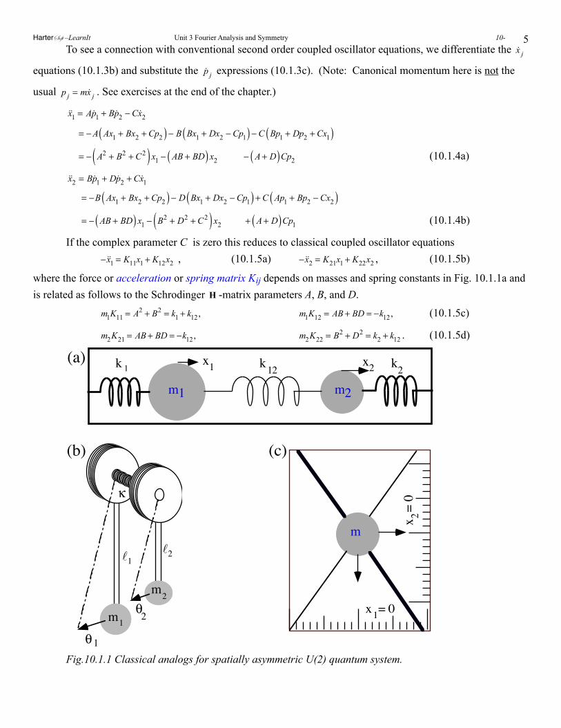
5 To see a connection with conventional second order coupled oscillator equations, we differentiate the
x j
equations (10.1.3b) and substitute the p j expressions (10.1.3c). (Note: Canonical momentum here is not the
usual p j = mx j . See exercises at the end of the chapter.)
x1 = Ap1 + Bp2 − C x2
= −A Ax1 + Bx2 + Cp2( ) − B Bx1 + Dx2 − Cp1( ) − C Bp1 + Dp2 + Cx1( )
= − A2 + B2 + C2( ) x1 − AB + BD( ) x2 − A+ D( )Cp2 (10.1.4a)
x2 = Bp1 + Dp2 + C x1
= −B Ax1 + Bx2 + Cp2( ) − D Bx1 + Dx2 − Cp1( ) + C Ap1 + Bp2 − Cx2( )
= − AB + BD( ) x1 − B2 + D2 + C2( ) x2 + A+ D( )Cp1 (10.1.4b)
If the complex parameter C is zero this reduces to classical coupled oscillator equations −x1 = K11x1 + K12x2 , (10.1.5a) −x2 = K21x1 + K22x2 , (10.1.5b)
where the force or acceleration or spring matrix Kij depends on masses and spring constants in Fig. 10.1.1a and is related as follows to the Schrodinger H -matrix parameters A, B, and D.
m1K11 = A2 + B2 = k1 + k12, m1K12 = AB + BD = −k12, (10.1.5c)
m2K21 = AB + BD = −k12, m2K22 = B2 + D2 = k2 + k12 . (10.1.5d)
x1k k kx21 12 2
m1 m2
(a)
θ1
θ2
κ
1
m
m2
2
(b)
1
x = 01
x =
02
m
(c)
Fig.10.1.1 Classical analogs for spatially asymmetric U(2) quantum system.
HarterSoft –LearnIt Unit 3 Fourier Analysis and Symmetry 10-
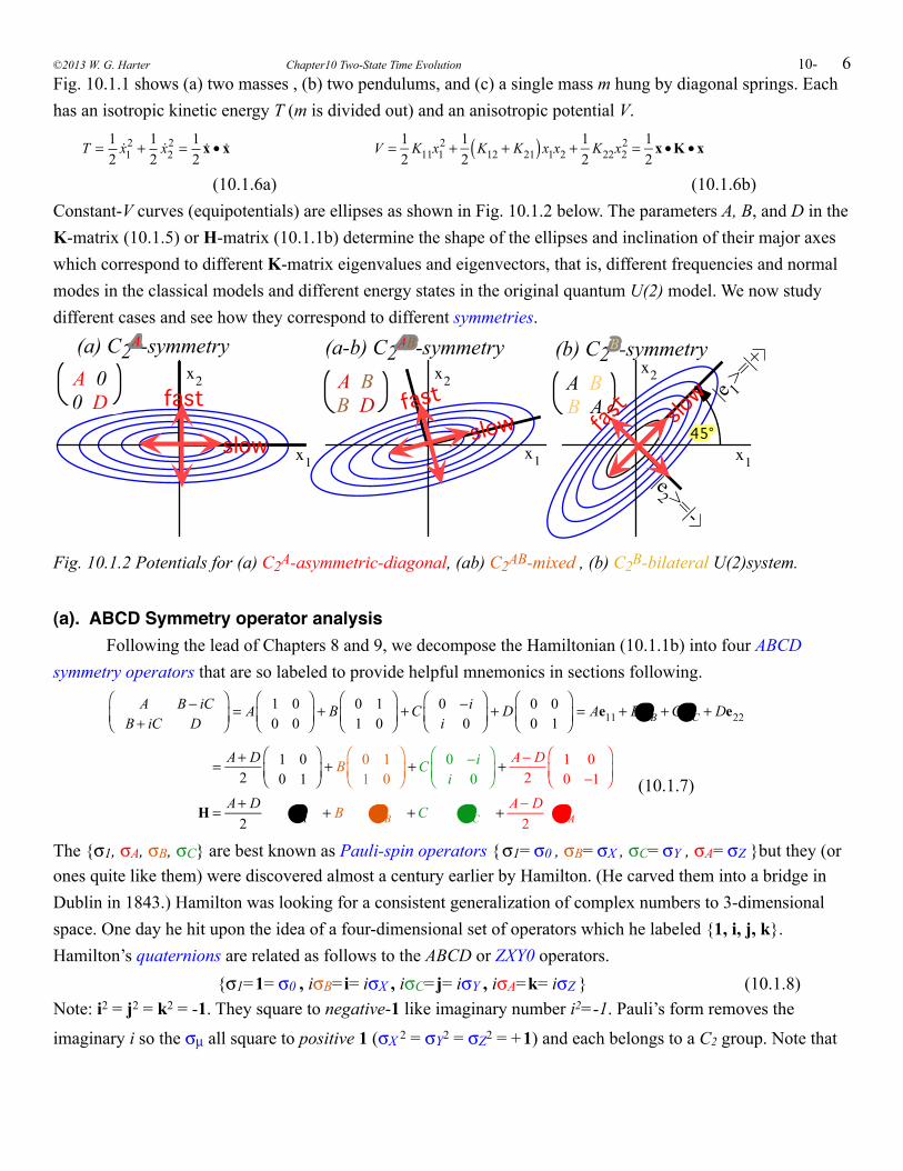
6Fig. 10.1.1 shows (a) two masses , (b) two pendulums, and (c) a single mass m hung by diagonal springs. Each has an isotropic kinetic energy T (m is divided out) and an anisotropic potential V.
T = 1
2x1
2 + 12x2
2 = 12x • x
V = 1
2K11x1
2 + 12
K12 + K21( )x1x2 +12
K22x22 = 1
2x •K • x
(10.1.6a) (10.1.6b)Constant-V curves (equipotentials) are ellipses as shown in Fig. 10.1.2 below. The parameters A, B, and D in the K-matrix (10.1.5) or H-matrix (10.1.1b) determine the shape of the ellipses and inclination of their major axes which correspond to different K-matrix eigenvalues and eigenvectors, that is, different frequencies and normal modes in the classical models and different energy states in the original quantum U(2) model. We now study different cases and see how they correspond to different symmetries.
x1
x2
x1
x2
4455°°x1
x2
(a-b) C2AABB-symmetry (b) C2BB-symmetryA 00 D
A BB D
A BB A
slow
fastslow
fast slow
fast |e 1
>=|+
|e2 >=|-
(a) C2AA-symmetry
Fig. 10.1.2 Potentials for (a) C2A-asymmetric-diagonal, (ab) C2AB-mixed , (b) C2B-bilateral U(2)system.
(a). ABCD Symmetry operator analysisFollowing the lead of Chapters 8 and 9, we decompose the Hamiltonian (10.1.1b) into four ABCD
symmetry operators that are so labeled to provide helpful mnemonics in sections following.
A B − iCB + iC D
⎛
⎝⎜⎞
⎠⎟= A 1 0
0 0⎛
⎝⎜⎞
⎠⎟+ B 0 1
1 0⎛
⎝⎜⎞
⎠⎟+C 0 −i
i 0⎛
⎝⎜⎞
⎠⎟+ D 0 0
0 1⎛
⎝⎜⎞
⎠⎟= Ae11 + BσB +CσC + De22
= A+ D2
1 00 1
⎛
⎝⎜⎞
⎠⎟+ B 0 1
1 0⎛
⎝⎜⎞
⎠⎟+C 0 −i
i 0⎛
⎝⎜⎞
⎠⎟+ A− D
21 00 −1
⎛
⎝⎜⎞
⎠⎟
H = A+ D2
σ1 + B σB +C σC + A− D2
σ A
(10.1.7)
The {σ1, σA, σB, σC} are best known as Pauli-spin operators { σ1= σ0 , σB= σX , σC= σY , σA= σZ }but they (or ones quite like them) were discovered almost a century earlier by Hamilton. (He carved them into a bridge in Dublin in 1843.) Hamilton was looking for a consistent generalization of complex numbers to 3-dimensional space. One day he hit upon the idea of a four-dimensional set of operators which he labeled {1, i, j, k}. Hamilton’s quaternions are related as follows to the ABCD or ZXY0 operators. {σ1=1= σ0 , iσB=i= iσX , iσC=j= iσY , iσA=k= iσZ } (10.1.8)Note: i2 = j2 = k2 = -1. They square to negative-1 like imaginary number i2=-1. Pauli’s form removes the
imaginary i so the σµ all square to positive 1 (σX 2 = σY2 = σZ2 = +1) and each belongs to a C2 group. Note that
©2013 W. G. Harter Chapter10 Two-State Time Evolution 10-
7our first operator σA (or Pauli’s third σZ ) is a difference σA =e11- e22 of elementary operators e11 and e22. σA is a group operator but ekk are not since they are projectors and do not have inverses. Now each C2 group C2A={1, σA}, C2B={1, σB}, and C2C={1, σC} is considered in turn. They are labeled A (asymmetric-diagonal), B (bilateral balanced beat), and C (circular) symmetry for reasons that will become clear. Each of them represents a different physical archetype and a different kind of dynamics. Mnemonic alliteration is used for pedagogical enhancement, particularly the C (circular) symmetry for which the following C-adjectives apply: complex, circular, chiral, cyclotron, Coriolis, centrifugal, curly, and circulating-current. The last symmetry adjective explains its important distinction and the coloring scheme used in formulae and illustrations. The A and B designations are colored the yellow, orange or red color of traffic signals for CAUTION, or STOP since these symmetries refer to real-standing waves. The green or blue-green GO signal color applies to the C (current-like) symmetry of imaginary or complex moving or galloping waves.
HarterSoft –LearnIt Unit 3 Fourier Analysis and Symmetry 10-
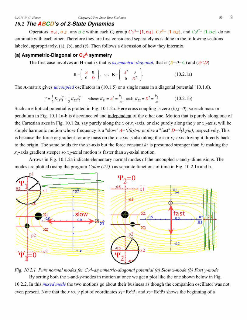
810.2 The ABCDʼs of 2-State Dynamics Operators σ A , σ B , any σ C within each C2 group C2A={1, σA}, C2B={1, σB}, and C2C={1, σC} do not commute with each other. Therefore they are first considered separately as is done in the following sections labeled, appropriately, (a), (b), and (c). Then follows a discussion of how they intermix.
(a) Asymmetric-Diagonal or C2A symmetry The first case involves an H-matrix that is asymmetric-diagonal, that is (B=0=C) and (A<D)
H = A 00 D
⎛
⎝⎜⎞
⎠⎟ , or: K = A2 0
0 D2
⎛
⎝⎜⎜
⎞
⎠⎟⎟
. (10.2.1a)
The A-matrix gives uncoupled oscillators in (10.1.5) or a single mass in a diagonal potential (10.1.6).
V = 1
2K11x1
2 + 12
K22x22 where: K11 = A2 =
k1m
, and: K22 = D2 =k2m
(10.2.1b)
Such an elliptical potential is plotted in Fig. 10.1.2a. Here cross coupling is zero (k12=0), so each mass or pendulum in Fig. 10.1.1a-b is disconnected and independent of the other one. Motion that is purely along one of the Cartesian axes in Fig. 10.1.2a, say purely along the x or x1-axis, or else purely along the y or x2-axis, will be simple harmonic motion whose frequency is a "slow" A=√(k1/m) or else a "fast" D=√(k2/m), respectively. This is because the force or gradient for any mass on the x -axis is also along the x or x1-axis driving it directly back to the origin. The same holds for the x2-axis but the force constant k2 is presumed stronger than k1 making the x2-axis gradient steeper so x2-axial motion is faster than x1-axial motion. Arrows in Fig. 10.1.2a indicate elementary normal modes of the uncoupled x-and y-dimensions. The modes are plotted (using the program Color U(2) ) as separate functions of time in Fig. 10.2.1a and b.
slow fast
x1
p1
x2
p2
x1
x2
p2
Ψ1
Ψ1= 0 Ψ2
Ψ2= 0
Fig. 10.2.1 Pure normal modes for C2A-asymmetric-diagonal potential (a) Slow x-mode (b) Fast y-mode By setting both the x-and-y-modes in motion at once we get a plot like the one shown below in Fig. 10.2.2. In this mixed mode the two motions go about their business as though the companion oscillator was not even present. Note that the x vs. y plot of coordinates x1=ReΨ1 and x2=ReΨ2 shows the beginning of a
©2013 W. G. Harter Chapter10 Two-State Time Evolution 10-
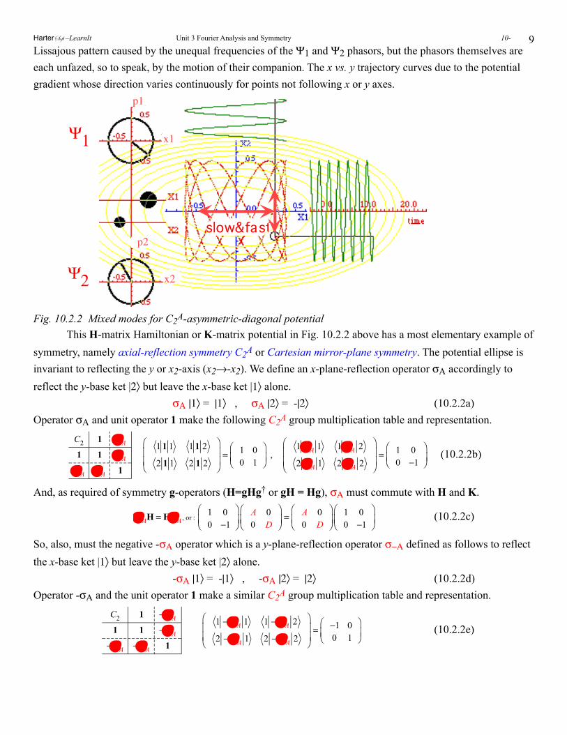
9Lissajous pattern caused by the unequal frequencies of the Ψ1 and Ψ2 phasors, but the phasors themselves are each unfazed, so to speak, by the motion of their companion. The x vs. y trajectory curves due to the potential gradient whose direction varies continuously for points not following x or y axes.
x1
p1
x2
p2slow&fast
Ψ1
Ψ2
Fig. 10.2.2 Mixed modes for C2A-asymmetric-diagonal potential This H-matrix Hamiltonian or K-matrix potential in Fig. 10.2.2 above has a most elementary example of symmetry, namely axial-reflection symmetry C2A or Cartesian mirror-plane symmetry. The potential ellipse is invariant to reflecting the y or x2-axis (x2→-x2). We define an x-plane-reflection operator σΑ accordingly to reflect the y-base ket |2〉 but leave the x-base ket |1〉 alone. σΑ |1〉 = |1〉 , σΑ |2〉 = -|2〉 (10.2.2a)Operator σΑ and unit operator 1 make the following C2A group multiplication table and representation.
C2 1 σ A
1 1 σ A
σ A σ A 1
1 1 1 1 1 2
2 1 1 2 1 2
⎛
⎝⎜⎜
⎞
⎠⎟⎟= 1 0
0 1⎛
⎝⎜⎞
⎠⎟ ,
1 σ A 1 1 σ A 2
2 σ A 1 2 σ A 2
⎛
⎝⎜⎜
⎞
⎠⎟⎟= 1 0
0 −1⎛
⎝⎜⎞
⎠⎟ (10.2.2b)
And, as required of symmetry g-operators (H=gHg† or gH = Hg), σΑ must commute with H and K.
σ AH = Hσ A , or :
1 00 −1
⎛
⎝⎜⎞
⎠⎟A 00 D
⎛
⎝⎜⎞
⎠⎟= A 0
0 D⎛
⎝⎜⎞
⎠⎟1 00 −1
⎛
⎝⎜⎞
⎠⎟ (10.2.2c)
So, also, must the negative -σΑ operator which is a y-plane-reflection operator σ−Α defined as follows to reflect the x-base ket |1〉 but leave the y-base ket |2〉 alone. -σΑ |1〉 = -|1〉 , -σΑ |2〉 = |2〉 (10.2.2d)Operator -σΑ and the unit operator 1 make a similar C2A group multiplication table and representation.
C2 1 −σ A
1 1 −σ A
−σ A −σ A 1
1 − σ A 1 1 − σ A 2
2 − σ A 1 2 − σ A 2
⎛
⎝⎜⎜
⎞
⎠⎟⎟= −1 0
0 1⎛
⎝⎜⎞
⎠⎟ (10.2.2e)
HarterSoft –LearnIt Unit 3 Fourier Analysis and Symmetry 10-
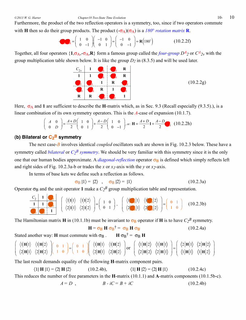
10Furthermore, the product of the two reflection operators is a symmetry, too, since if two operators commute with H then so do their group products. The product (-σΑ)(σΑ) is a 180° rotation matrix R.
−σ Aσ A = 1 0
0 −1⎛
⎝⎜⎞
⎠⎟−1 00 1
⎛
⎝⎜⎞
⎠⎟= −1 0
0 −1⎛
⎝⎜⎞
⎠⎟= R 180( ) (10.2.2f)
Together, all four operators {1,σΑ,-σΑ,R} form a famous group called the four-group DA2 or CA2v with the group multiplication table shown below. It is like the group D2 in (8.3.5) and will be used later.
C2v 1 σ A −σ A R
1 1 σ A −σ A R
σ A σ A 1 R −σ A
−σ A −σ A R 1 σ A
R R −σ A σ A 1
(10.2.2g)
Here, σΑ and 1 are sufficient to describe the H-matrix which, as in Sec. 9.3 (Recall especially (9.3.5).), is a linear combination of its own symmetry operators. This is the A-case of expansion (10.1.7).
A 00 D
⎛
⎝⎜⎞
⎠⎟= A+ D
21 00 1
⎛
⎝⎜⎞
⎠⎟+ A− D
21 00 −1
⎛
⎝⎜⎞
⎠⎟, or : H = A+ D
21+ A− D
2σ A (10.2.2h)
(b) Bilateral or C2B symmetry The next case-B involves identical coupled oscillators such are shown in Fig. 10.2.3 below. These have a symmetry called bilateral or C2B symmetry. We should be very familiar with this symmetry since it is the only one that our human bodies approximate. A diagonal-reflection operator σΒ is defined which simply reflects left and right sides of Fig. 10.2.3a-b or trades the x or x1-axis with the y or x2-axis. In terms of base kets we define such a reflection as follows. σΒ |1〉 = |2〉 , σΒ |2〉 = |1〉 (10.2.3a)Operator σΒ and the unit operator 1 make a C2B group multiplication table and representation.
C2 1 σΒ
1 1 σΒ
σΒ σΒ 1
1 1 1 1 1 2
2 1 1 2 1 2
⎛
⎝⎜⎜
⎞
⎠⎟⎟= 1 0
0 1⎛
⎝⎜⎞
⎠⎟ ,
1 σΒ 1 1 σΒ 2
2 σΒ 1 2 σΒ 2
⎛
⎝⎜⎜
⎞
⎠⎟⎟= 0 1
1 0⎛
⎝⎜⎞
⎠⎟ (10.2.3b)
The Hamiltonian matrix H in (10.1.1b) must be invariant to σΒ operator if H is to have C2B symmetry. H = σΒ H σΒ† = σΒ H σΒ (10.2.4a)Stated another way: H must commute with σΒ . H σΒ† = σΒ H
1 H 1 1 H 2
2 H 1 2 H 2
⎛
⎝⎜⎜
⎞
⎠⎟⎟
0 11 0
⎛
⎝⎜⎞
⎠⎟= 0 1
1 0⎛
⎝⎜⎞
⎠⎟1 H 1 1 H 2
2 H 1 2 H 2
⎛
⎝⎜⎜
⎞
⎠⎟⎟
or
1 H 2 1 H 1
2 H 2 2 H 1
⎛
⎝⎜⎜
⎞
⎠⎟⎟=
2 H 1 2 H 2
1 H 1 1 H 2
⎛
⎝⎜⎜
⎞
⎠⎟⎟
The last result demands equality of the following H-matrix component pairs. 〈1| H |1〉 = 〈2| H |2〉 (10.2.4b), 〈1| H |2〉 = 〈2| H |1〉 (10.2.4c)This reduces the number of free parameters in the H-matrix (10.1.1) and A-matrix components (10.1.5b-c). A = D , B - iC = B + iC (10.2.4b)
©2013 W. G. Harter Chapter10 Two-State Time Evolution 10-
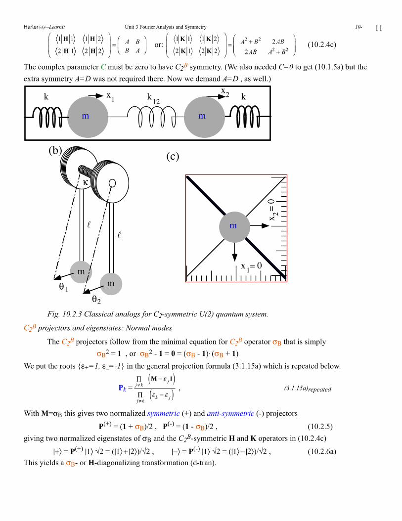
11
1 H 1 1 H 2
2 H 1 2 H 2
⎛
⎝⎜⎜
⎞
⎠⎟⎟= A B
B A⎛
⎝⎜⎞
⎠⎟ or:
1 K 1 1 K 2
2 K 1 2 K 2
⎛
⎝⎜⎜
⎞
⎠⎟⎟= A2 + B2 2AB
2AB A2 + B2
⎛
⎝⎜⎜
⎞
⎠⎟⎟
(10.2.4c)
The complex parameter C must be zero to have C2B symmetry. (We also needed C=0 to get (10.1.5a) but the extra symmetry A=D was not required there. Now we demand A=D , as well.)
x1k k kx2
12
m m
x = 01x
= 0
2
m
θ1θ2
κ
mm
(b) (c)
Fig. 10.2.3 Classical analogs for C2-symmetric U(2) quantum system.
C2B projectors and eigenstates: Normal modes
The C2B projectors follow from the minimal equation for C2B operator σΒ that is simply σΒ2 = 1 , or σΒ2 - 1 = 0 = (σΒ - 1). (σΒ + 1) We put the roots {ε+=1, ε_=-1} in the general projection formula (3.1.15a) which is repeated below.
Pk =
j≠k∏ M − ε j1( )j≠k∏ εk − ε j( ) , (3.1.15a)repeated
With M=σΒ this gives two normalized symmetric (+) and anti-symmetric (-) projectors
P(+) = (1 + σΒ)/2 , P(-) = (1 - σΒ)/2 , (10.2.5)giving two normalized eigenstates of σΒ and the C2B-symmetric H and K operators in (10.2.4c)
|+〉 = P(+) |1〉 √2 = (|1〉 + |2〉)/√2 , |−〉 = P(-) |1〉 √2 = (|1〉 − |2〉)/√2 , (10.2.6a) This yields a σΒ- or H-diagonalizing transformation (d-tran).
HarterSoft –LearnIt Unit 3 Fourier Analysis and Symmetry 10-
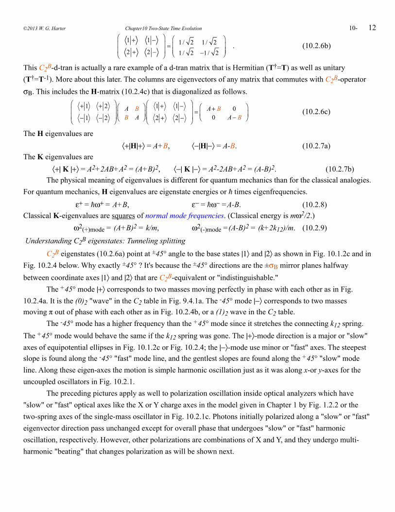
12
1 + 1 −
2 + 2 −
⎛
⎝⎜⎜
⎞
⎠⎟⎟= 1 / 2 1 / 2
1 / 2 −1 / 2
⎛
⎝⎜⎜
⎞
⎠⎟⎟
. (10.2.6b)
This C2B-d-tran is actually a rare example of a d-tran matrix that is Hermitian (T†=T) as well as unitary (T†=T-1). More about this later. The columns are eigenvectors of any matrix that commutes with C2B-operator σΒ. This includes the H-matrix (10.2.4c) that is diagonalized as follows.
+ 1 + 2
− 1 − 2
⎛
⎝⎜⎜
⎞
⎠⎟⎟
A BB A
⎛
⎝⎜⎞
⎠⎟1 + 1 −
2 + 2 −
⎛
⎝⎜⎜
⎞
⎠⎟⎟= A+ B 0
0 A− B⎛
⎝⎜⎞
⎠⎟ (10.2.6c)
The H eigenvalues are 〈+|H|+〉 = A+B, 〈−|H|−〉 = A-B. (10.2.7a)The K eigenvalues are 〈+| K |+〉 = A2+2AB+A2 = (A+B)2, 〈−| K |−〉 = A2-2AB+A2 = (A-B)2. (10.2.7b) The physical meaning of eigenvalues is different for quantum mechanics than for the classical analogies. For quantum mechanics, H eigenvalues are eigenstate energies or times eigenfrequencies.
ε+ = ω+ = A+B, ε− = ω− =A-B. (10.2.8)Classical K-eigenvalues are squares of normal mode frequencies. (Classical energy is mω2/2.) ω2(+)mode = (A+B)2 = k/m, ω2(-)mode =(A-B)2 = (k+2k12)/m. (10.2.9)
Understanding C2B eigenstates: Tunneling splitting
C2B eigenstates (10.2.6a) point at ±45° angle to the base states |1〉 and |2〉 as shown in Fig. 10.1.2c and in Fig. 10.2.4 below. Why exactly ±45° ? It's because the ±45° directions are the ±σΒ mirror planes halfway between coordinate axes |1〉 and |2〉 that are C2B-equivalent or "indistinguishable." The +45° mode |+〉 corresponds to two masses moving perfectly in phase with each other as in Fig. 10.2.4a. It is the (0)2 "wave" in the C2 table in Fig. 9.4.1a. The -45° mode |−〉 corresponds to two masses moving π out of phase with each other as in Fig. 10.2.4b, or a (1)2 wave in the C2 table. The -45° mode has a higher frequency than the +45° mode since it stretches the connecting k12 spring. The +45° mode would behave the same if the k12 spring was gone. The |+〉-mode direction is a major or "slow" axes of equipotential ellipses in Fig. 10.1.2c or Fig. 10.2.4; the |−〉-mode use minor or "fast" axes. The steepest slope is found along the -45° "fast" mode line, and the gentlest slopes are found along the +45° "slow" mode line. Along these eigen-axes the motion is simple harmonic oscillation just as it was along x-or y-axes for the uncoupled oscillators in Fig. 10.2.1. The preceding pictures apply as well to polarization oscillation inside optical analyzers which have "slow" or "fast" optical axes like the X or Y charge axes in the model given in Chapter 1 by Fig. 1.2.2 or the two-spring axes of the single-mass oscillator in Fig. 10.2.1c. Photons initially polarized along a "slow" or "fast" eigenvector direction pass unchanged except for overall phase that undergoes "slow" or "fast" harmonic oscillation, respectively. However, other polarizations are combinations of X and Y, and they undergo multi-harmonic "beating" that changes polarization as will be shown next.
©2013 W. G. Harter Chapter10 Two-State Time Evolution 10-
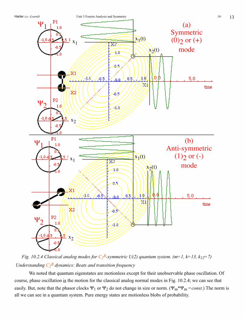
13
x1
x2
x1(t)
x2(t)
x1
x2
x1(t)
x2(t)
(a)Symmetric(0)2 or (+)
mode
(b)Anti-symmetric
(1)2 or (-)mode
Ψ1
Ψ1
Ψ2
Ψ2
Fig. 10.2.4 Classical analog modes for C2B-symmetric U(2) quantum system. (m=1, k=13, k12=7)
Understanding C2B dynamics: Beats and transition frequency
We noted that quantum eigenstates are motionless except for their unobservable phase oscillation. Of course, phase oscillation is the motion for the classical analog normal modes in Fig. 10.2.4; we can see that easily. But, note that the phasor clocks Ψ1 or Ψ2 do not change in size or norm. (Ψm*Ψm =const.) The norm is all we can see in a quantum system. Pure energy states are motionless blobs of probability.
HarterSoft –LearnIt Unit 3 Fourier Analysis and Symmetry 10-
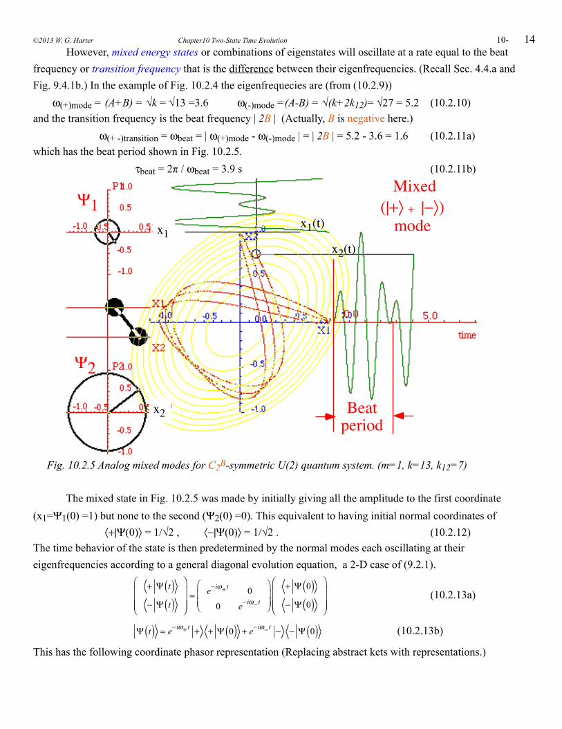
14 However, mixed energy states or combinations of eigenstates will oscillate at a rate equal to the beat frequency or transition frequency that is the difference between their eigenfrequencies. (Recall Sec. 4.4.a and Fig. 9.4.1b.) In the example of Fig. 10.2.4 the eigenfrequecies are (from (10.2.9)) ω(+)mode = (A+B) = √k = √13 =3.6 ω(-)mode =(A-B) = √(k+2k12)= √27 = 5.2 (10.2.10)and the transition frequency is the beat frequency | 2B | (Actually, B is negative here.) ω(+ -)transition = ωbeat = | ω(+)mode - ω(-)mode | = | 2B | = 5.2 - 3.6 = 1.6 (10.2.11a)which has the beat period shown in Fig. 10.2.5. τbeat = 2π / ωbeat = 3.9 s (10.2.11b)
x1
x2
x1(t)
x2(t)
Mixed(|+〉 + |−〉)
mode
Beatperiod
Ψ1
Ψ2
Fig. 10.2.5 Analog mixed modes for C2B-symmetric U(2) quantum system. (m=1, k=13, k12=7)
The mixed state in Fig. 10.2.5 was made by initially giving all the amplitude to the first coordinate (x1=Ψ1(0) =1) but none to the second (Ψ2(0) =0). This equivalent to having initial normal coordinates of 〈+|Ψ(0)〉 = 1/√2 , 〈−|Ψ(0)〉 = 1/√2 . (10.2.12)The time behavior of the state is then predetermined by the normal modes each oscillating at their eigenfrequencies according to a general diagonal evolution equation, a 2-D case of (9.2.1).
+ Ψ t( )− Ψ t( )
⎛
⎝
⎜⎜⎜
⎞
⎠
⎟⎟⎟= e−iω+ t 0
0 e−iω− t
⎛
⎝⎜⎜
⎞
⎠⎟⎟
+ Ψ 0( )− Ψ 0( )
⎛
⎝
⎜⎜⎜
⎞
⎠
⎟⎟⎟
(10.2.13a)
Ψ t( ) = e−iω+ t + + Ψ 0( ) + e−iω− t − − Ψ 0( ) (10.2.13b)
This has the following coordinate phasor representation (Replacing abstract kets with representations.)
©2013 W. G. Harter Chapter10 Two-State Time Evolution 10-
15
Ψ t( ) = e−iω+ t + + Ψ 0( ) + e−iω− t − − Ψ 0( )Ψ1 t( )Ψ2 t( )
⎛
⎝⎜⎜
⎞
⎠⎟⎟=
1 Ψ t( )2 Ψ t( )
⎛
⎝
⎜⎜⎜
⎞
⎠
⎟⎟⎟= e−iω+ t 1 +
2 +
⎛
⎝⎜⎜
⎞
⎠⎟⎟
+ Ψ 0( ) + e−iω− t 1 −
2 −
⎛
⎝⎜⎜
⎞
⎠⎟⎟
− Ψ 0( )
= e−iω+ t 1 / 21 / 2
⎛
⎝⎜⎜
⎞
⎠⎟⎟
1 / 2 + e−iω− t 1 / 2−1 / 2
⎛
⎝⎜⎜
⎞
⎠⎟⎟
1 / 2
(10.2.14a)
This reduces to the following. (Recall the use of the expo-sine identity in (4.4.3c).)
Ψ1 t( )Ψ2 t( )
⎛
⎝⎜⎜
⎞
⎠⎟⎟= 1
2e−iω+ t + e−iω− t
e−iω+ t − e−iω− t
⎛
⎝⎜⎜
⎞
⎠⎟⎟= e−i(ω+ +ω− )t / 2
2e−i(ω+ −ω− )t / 2 + ei(ω+ −ω− )t / 2
e−i(ω+ −ω− )t / 2 − ei(ω+ −ω− )t / 2
⎛
⎝⎜⎜
⎞
⎠⎟⎟
= e−i(ω+ +ω− )t / 2 cos (ω+ −ω− )t / 2⎡⎣ ⎤⎦i sin (ω+ −ω− )t / 2⎡⎣ ⎤⎦
⎛
⎝⎜⎜
⎞
⎠⎟⎟
(10.2.14b)
According to this, the bottom Ψ2(t) phasor amplitude grows sinusoidally from zero to its maximum with a rate that is half the beat frequency. ωhalf-beat = ωbeat /2 = | ω(+)mode - ω(-)mode |/2 (10.2.15)As seen in Fig. 10.2.5, the bottom Ψ2(t) phasor goes around 90° behind the top Ψ1(t) phasor. That is the i factor in the Ψ2(t) part of (10.2.14b). The overall phase rotates at an average rate ωaverage = ( ω(+)mode + ω(-)mode )/2. (10.2.16)Then, just as the bottom Ψ2(t) phasor passes its maximum, it moves 90° ahead of the top Ψ1(t) phasor that has just gone through zero and starts to grow. The bottom Ψ2(t) phasor returns to zero amplitude every beat period τbeat given by (10.2.11b) just as the top Ψ1(t) phasor reaches its maximum amplitude. The relative phase between the two phasors is important classically as well as in the quantum analog. Whichever phasor is ahead is the one feeding energy to the other that grows while its feeder shrinks. One should recall an important resonance theorem: (Prove this if it's new to you. See exercises.) Power transfer between two isochronous linearly connected oscillators is proportional to the product of their amplitudes and the sine of their relative phase. A relative phase of 90° gives the best possible work rate. This type of resonance transfer is important in quantum mechanics. A relative phase of 0° or 180° gives no transfer, as in a classical normal mode or a quantum stationary state; having no net energy gain or loss by individual parts makes them stationary. Another way to visualize beats is by analogy to optical polarization-wave-plates introduced in Fig. 1.3.6b. One quarter of a beat corresponds to a quarter wave plate. The effect is to convert X-polarization into right circular polarization as shown below in Fig. 10.2.6a. A half-beat converts X=x1 to Y=x2 as in Fig. 10.2.6b and corresponds to a half-wave plate as shown below in Fig. 10.2.6b. For this example, the coupling constant 2B = √k -√(k+2k12) is reduced from -1.6 in (10.2.11a) to -0.26 to slow the beat from 3 periods to about 18. Real wave-plate beats take millions of periods so 18 is still way too fast.
HarterSoft –LearnIt Unit 3 Fourier Analysis and Symmetry 10-
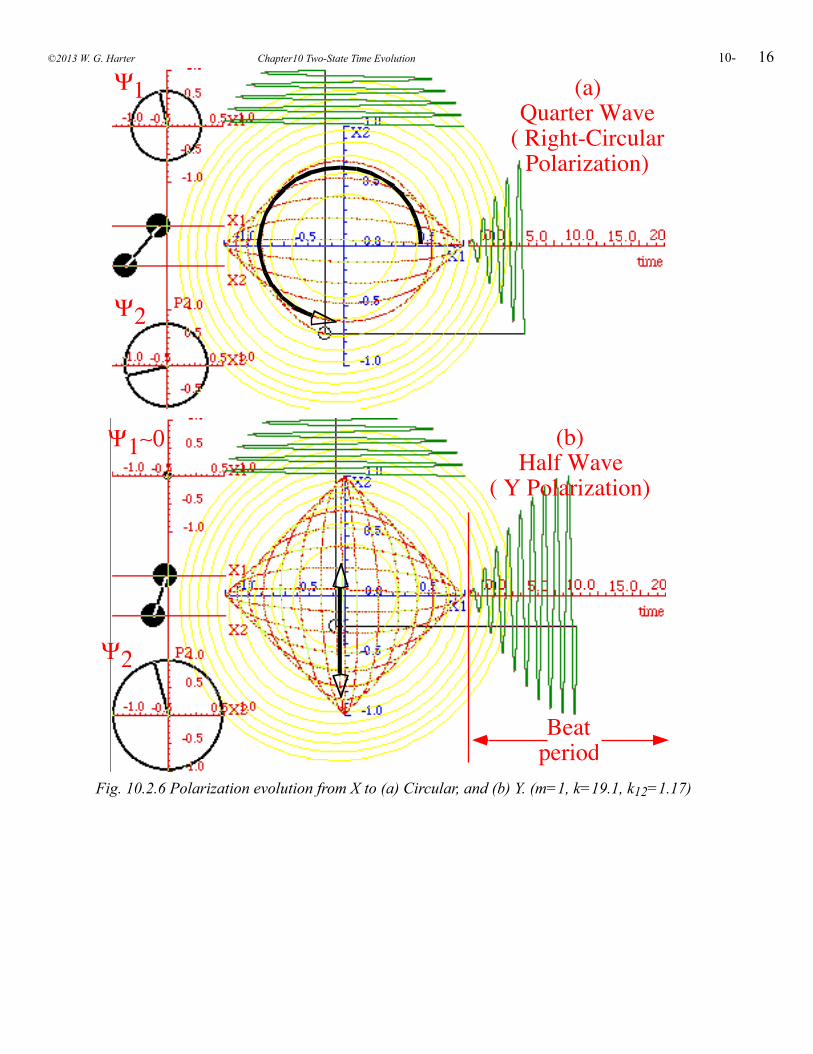
16
(a)Quarter Wave
( Right-CircularPolarization)
Ψ1
Ψ2
(b)Half Wave
( Y Polarization)
Beatperiod
Ψ1∼0
Ψ2
Fig. 10.2.6 Polarization evolution from X to (a) Circular, and (b) Y. (m=1, k=19.1, k12=1.17)
©2013 W. G. Harter Chapter10 Two-State Time Evolution 10-
17(c) Circular or C2C symmetry Now we consider the very different case in which all parameters are zero except C. Then a continuous circular rotational C∞ symmetry or R(2) symmetry is present. The reflection symmetry associated with the C-parameter is called C2C or R(2)=C∞. C2C-symmetry states are characterized by circularity and chirality or "handedness." Now the circular motion in Fig. 10.2.6a is an eigenstate.
C∞-symmetry means a two-by-two Hermitian Hamiltonian
H† = H( ) matrix operator
H =1 H 1 1 H 2
2 H 1 2 H 2
⎛
⎝⎜⎜
⎞
⎠⎟⎟= A B − iC
B + iC D⎛
⎝⎜⎞
⎠⎟. (10.1.1b)repeated
commutes with any rotation operator R(φ) defined as follows. (Recall (2.2.1) in Chapter 2.) R(φ) |1〉 = cos φ |1〉 + sin φ |2〉 , R(φ) |2〉 = -sin φ |1〉 + cos φ |2〉 (10.2.18a)Rotation R(φ) has the following R(2)=C∞ group multiplication rule and C∞ representation.
R φ( ) ⋅R φ '( )=R φ + φ '( ) , 1 R 1 1 R 2
2 R 1 2 R 2
⎛
⎝⎜⎜
⎞
⎠⎟⎟=
cosφ − sinφsinφ cosφ
⎛
⎝⎜⎜
⎞
⎠⎟⎟
(10.2.18b)
Since matrix H must commute with R(φ) for all φ, it must also commute with the derivative of R(φ) at zero rotation (φ=0 and R(0) = 1 ). The derivative of a transformation operator near 1 is called the generator G of the operator. The generator of the rotation R(φ) is as follows.
G=∂∂φ
R φ( ) φ=0 =− sinφ − cosφcosφ − sinφ
⎛
⎝⎜⎜
⎞
⎠⎟⎟φ=0
= 0 −11 0
⎛
⎝⎜⎞
⎠⎟, or: R φ( ) = R 0( )eφG = eφG (10.2.18c)
The set R(2)=C∞ of all R(φ) operators is an example of continuous or Lie group symmetry. It is very much like the "empty time" symmetry made of all time evolution operators U(t)=e-iH t. The generator of the evolution operators U(t) is the Hamiltonian H itself. Multiplying R(φ) generator G by i and gives a third C2C-Hamilton-Pauli reflection operator σC .
σC= 0 −i
i 0⎛
⎝⎜⎞
⎠⎟=iG, where: σC
†σC = σC2 = 1 (10.2.18d)
The i makes σC Hermitian-unitary like σA and σB, and gives it a (-1) determinant.(det|σC|=-1) So σC has similar properties to a reflection operator, but it sure doesn’t look like one!. Reflection operator σC for circular C2C-symmetry is imaginary unlike σA and σB that are real. However, the C2C rotation matrices R(φ) are all real, but we will find imaginary rotations associated with C2A-symmetry or C2B-symmetry. Imaginary rotations are Lorentz transformations! More on this later. The physical idea is that C2A or C2B-symmetries are associated with "static" or standing wave states that have a real (±)-reflection symmetry about their nodes or anti-nodes. For the classical analogies the nodes corresponded to normal modes or polarization planes. The nodes, modes, or planes sit in different places depending on whether it is C2A, C2AB, or C2B-symmetry, but they must sit still. In contrast, states having C2C-symmetry are moving waves that have no fixed nodes or anti-nodes. Instead, they are characterized by a real (±)-direction of motion and a chirality of left or right handed motion.
HarterSoft –LearnIt Unit 3 Fourier Analysis and Symmetry 10-
18This is why C2C-rotation operators are real while it is the reflection operators that are real for C2A, C2AB, or C2B-symmetries. The former has a constant momentum, the latter a constant position. Commutation with reflection σC or generator G yields C2C-symmetry restrictions on H-matrices.
H ⋅ G = G ⋅H
1 H 1 1 H 2
2 H 1 2 H 2
⎛
⎝⎜⎜
⎞
⎠⎟⎟
0 −11 0
⎛
⎝⎜⎞
⎠⎟= 0 −1
1 0
⎛
⎝⎜⎞
⎠⎟1 H 1 1 H 2
2 H 1 2 H 2
⎛
⎝⎜⎜
⎞
⎠⎟⎟
1 H 2 − 1 H 1
2 H 2 − 2 H 1
⎛
⎝⎜⎜
⎞
⎠⎟⎟=
− 2 H 1 − 2 H 2
1 H 1 1 H 2
⎛
⎝⎜⎜
⎞
⎠⎟⎟
(10.2.19a)
Thus, R(2)=C∞ or C2C-symmetry demands the following for H matrix components. 〈1| H |1〉 = 〈2| H |2〉 , 〈1| H |2〉 = -〈2| H |1〉 (10.2.19b)For the H example (10.1.1b) we have A = D , B - iC = -(B + iC ) (10.2.19c)
so only two free parameters remain.
1 H 1 1 H 2
2 H 1 2 H 2
⎛
⎝⎜⎜
⎞
⎠⎟⎟= A −iC
iC A⎛
⎝⎜⎞
⎠⎟ (10.2.19d)
This H matrix is easy to diagonalize, but let's use symmetry projection just to get some more practice.
R(2)=C∞ projectors and C2C eigenstates
The R(2)=C∞ projectors follow from the secular equation for R(2)=C∞ operator R(φ) which is ε2 - (trace R(φ)) ε + (det R(φ)) = 0 = ε2 - (2cos φ) ε + 1 (10.2.20)The ±eigenvalues are labeled L and R for "Left" and "Right" for reasons that we'll see below.
εL = cosφ + cosφ2 −1 = cosφ + isinφ = eiφ (10.2.21a)
εR = cosφ − cosφ2 −1 = cosφ − i sinφ = e−iφ (10.2.21b)
Substituting the roots {εL=eiφ, εR=e-iφ} of M=R(φ) in the projection formula ((3.1.15) repeated below)
Pk =
j≠k∏ M − ε j1( )j≠k∏ εk − ε j( ) , (3.1.15a)repeated
gives two normalized projectors
P( L) =
cosφ − e−iφ − sinφ
sinφ cosφ − e−iφ
⎛
⎝⎜⎜
⎞
⎠⎟⎟
eiφ − e−iφ , P( R) =
cosφ − eiφ − sinφ
sinφ cosφ − eiφ
⎛
⎝⎜⎜
⎞
⎠⎟⎟
e−iφ − eiφ
=
i sinφ − sinφsinφ i sinφ
⎛
⎝⎜⎜
⎞
⎠⎟⎟
2i sinφ=
1 i−i 1
⎛
⎝⎜⎞
⎠⎟
2 , =
i sinφ − sinφsinφ i sinφ
⎛
⎝⎜⎜
⎞
⎠⎟⎟
−2i sinφ=
1 −ii 1
⎛
⎝⎜⎞
⎠⎟
2
, (10.2.22)
which in turn, give two normalized eigenstates of the R(2) -symmetric H operator in (10.2.19d)
|L〉 = P(L) |1〉 √2 = (|1〉 −i |2〉)/√2 , |R〉 = P(R) |1〉 √2 = (|1〉 +i |2〉)/√2 , (10.2.23a) and a diagonalizing transformation
©2013 W. G. Harter Chapter10 Two-State Time Evolution 10-
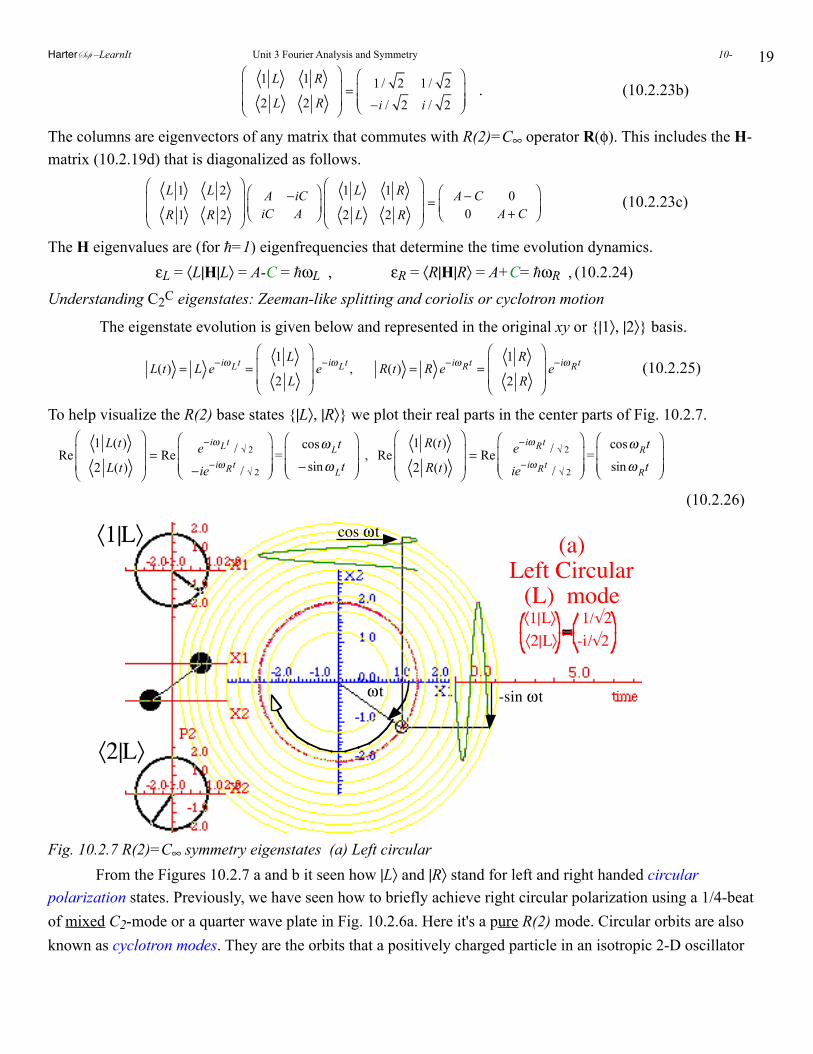
19
1 L 1 R
2 L 2 R
⎛
⎝⎜⎜
⎞
⎠⎟⎟= 1 / 2 1 / 2
−i / 2 i / 2
⎛
⎝⎜⎜
⎞
⎠⎟⎟
. (10.2.23b)
The columns are eigenvectors of any matrix that commutes with R(2)=C∞ operator R(φ). This includes the H-matrix (10.2.19d) that is diagonalized as follows.
L 1 L 2
R 1 R 2
⎛
⎝⎜⎜
⎞
⎠⎟⎟
A −iCiC A
⎛
⎝⎜⎞
⎠⎟1 L 1 R
2 L 2 R
⎛
⎝⎜⎜
⎞
⎠⎟⎟= A− C 0
0 A+ C⎛
⎝⎜⎞
⎠⎟ (10.2.23c)
The H eigenvalues are (for =1) eigenfrequencies that determine the time evolution dynamics. εL = 〈L|H|L〉 = A-C = ωL , εR = 〈R|H|R〉 = A+C= ωR , (10.2.24)
Understanding C2C eigenstates: Zeeman-like splitting and coriolis or cyclotron motion
The eigenstate evolution is given below and represented in the original xy or {|1〉, |2〉} basis.
L(t) = L e−iωLt =1 L
2 L
⎛
⎝⎜⎜
⎞
⎠⎟⎟
e−iωLt , R(t) = R e−iωRt =1 R
2 R
⎛
⎝⎜⎜
⎞
⎠⎟⎟
e−iωRt (10.2.25)
To help visualize the R(2) base states {|L〉, |R〉} we plot their real parts in the center parts of Fig. 10.2.7.
Re1 L(t)
2 L(t)
⎛
⎝⎜⎜
⎞
⎠⎟⎟= Re e−iωLt / √ 2
−ie−iωRt / √ 2
⎛
⎝⎜⎜
⎞
⎠⎟⎟
=cosω Lt
− sinω Lt
⎛
⎝⎜⎜
⎞
⎠⎟⎟
, Re1 R(t)
2 R(t)
⎛
⎝⎜⎜
⎞
⎠⎟⎟= Re e−iωRt / √ 2
ie−iωRt / √ 2
⎛
⎝⎜⎜
⎞
⎠⎟⎟
=cosωRt
sinωRt
⎛
⎝⎜⎜
⎞
⎠⎟⎟
(10.2.26)
ω t -sin ω t
cos ω t(a)
Left Circular(L) mode
〈1|L〉
〈2|L〉
〈1|L〉 1/√2〈2|L〉 -i/√2
Fig. 10.2.7 R(2)=C∞ symmetry eigenstates (a) Left circular From the Figures 10.2.7 a and b it seen how |L〉 and |R〉 stand for left and right handed circular polarization states. Previously, we have seen how to briefly achieve right circular polarization using a 1/4-beat of mixed C2-mode or a quarter wave plate in Fig. 10.2.6a. Here it's a pure R(2) mode. Circular orbits are also known as cyclotron modes. They are the orbits that a positively charged particle in an isotropic 2-D oscillator
HarterSoft –LearnIt Unit 3 Fourier Analysis and Symmetry 10-
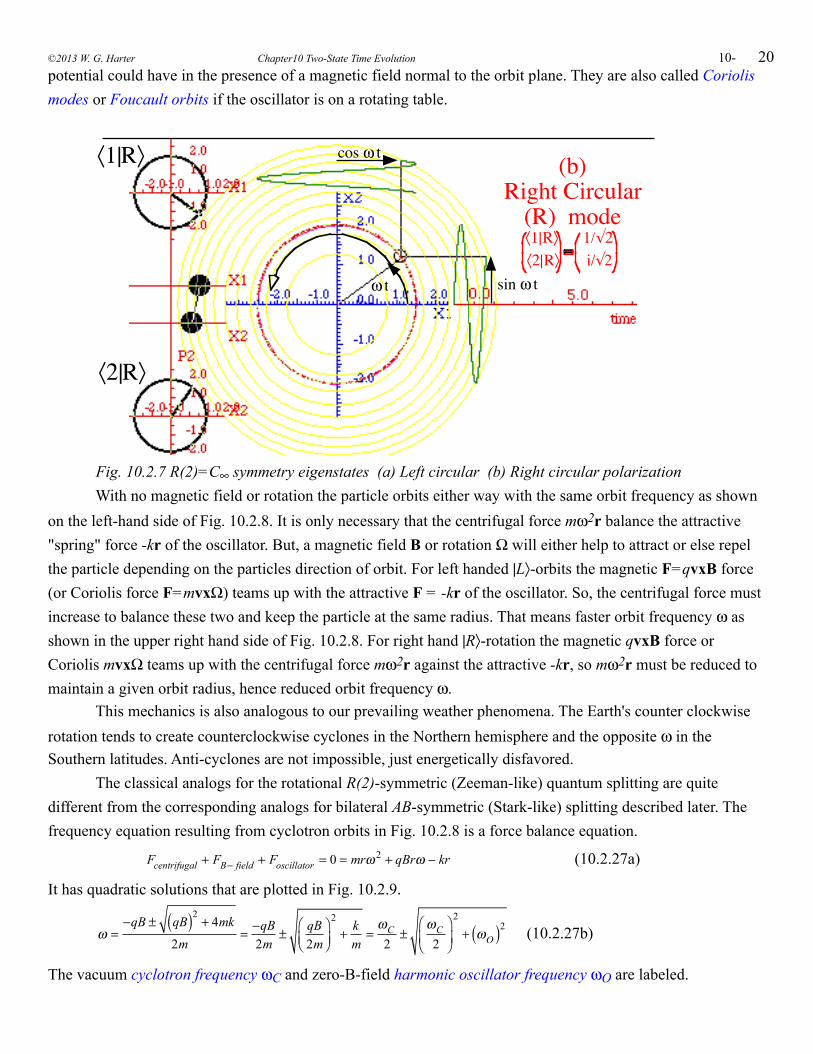
20potential could have in the presence of a magnetic field normal to the orbit plane. They are also called Coriolis modes or Foucault orbits if the oscillator is on a rotating table.
ω t sin ω t
cos ω t(b)
Right Circular(R) mode
〈1|R〉
〈2|R〉
〈1|R〉 1/√2〈2|R〉 i/√2
Fig. 10.2.7 R(2)=C∞ symmetry eigenstates (a) Left circular (b) Right circular polarization With no magnetic field or rotation the particle orbits either way with the same orbit frequency as shown on the left-hand side of Fig. 10.2.8. It is only necessary that the centrifugal force mω2r balance the attractive "spring" force -kr of the oscillator. But, a magnetic field B or rotation Ω will either help to attract or else repel the particle depending on the particles direction of orbit. For left handed |L〉-orbits the magnetic F=qvxB force (or Coriolis force F=mvxΩ) teams up with the attractive F = -kr of the oscillator. So, the centrifugal force must increase to balance these two and keep the particle at the same radius. That means faster orbit frequency ω as shown in the upper right hand side of Fig. 10.2.8. For right hand |R〉-rotation the magnetic qvxB force or Coriolis mvxΩ teams up with the centrifugal force mω2r against the attractive -kr, so mω2r must be reduced to maintain a given orbit radius, hence reduced orbit frequency ω. This mechanics is also analogous to our prevailing weather phenomena. The Earth's counter clockwise rotation tends to create counterclockwise cyclones in the Northern hemisphere and the opposite ω in the Southern latitudes. Anti-cyclones are not impossible, just energetically disfavored. The classical analogs for the rotational R(2)-symmetric (Zeeman-like) quantum splitting are quite different from the corresponding analogs for bilateral AB-symmetric (Stark-like) splitting described later. The frequency equation resulting from cyclotron orbits in Fig. 10.2.8 is a force balance equation.
Fcentrifugal + FB− field + Foscillator = 0 = mrω 2 + qBrω − kr (10.2.27a)
It has quadratic solutions that are plotted in Fig. 10.2.9.
ω =
−qB ± qB( )2 + 4mk
2m= −qB
2m± qB
2m⎛⎝⎜
⎞⎠⎟
2
+ km
=ωC2
±ωC2
⎛
⎝⎜⎞
⎠⎟
2
+ ωO( )2 (10.2.27b)
The vacuum cyclotron frequency ωC and zero-B-field harmonic oscillator frequency ωO are labeled.
©2013 W. G. Harter Chapter10 Two-State Time Evolution 10-
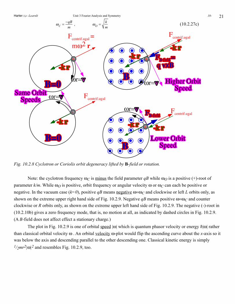
21
ωC = −qB
m , ωO = k
m (10.2.27c)
--kk rr
--kk rr
--kk rr
--kk rr FFBB ffiieelldd ==qq vvxxBB
Fcentrif.ugal =mω2 r
Fcentrif.ugalFFBB ffiieelldd
Fcentrif.ugal
Fcentrif.ugal
ωr=vv
--kk rr
--kk rr+
++
+
BB
BBBB==00
BB==00ωr=vv
ωr=vv
ωr=vv
HHiigghheerr OOrrbbiittSSppeeeedd
LLoowweerr OOrrbbiittSSppeeeedd
SSaammee OOrrbbiittSSppeeeeddss
Fig. 10.2.8 Cyclotron or Coriolis orbit degeneracy lifted by B-field or rotation.
Note: the cyclotron frequency ωC is minus the field parameter qB while ωO is a positive (+)-root of parameter k/m. While ωO is positive, orbit frequency or angular velocity ω or ωC can each be positive or negative. In the vacuum case (k=0), positive qB means negative ω=ωC and clockwise or left L orbits only, as shown on the extreme upper right hand side of Fig. 10.2.9. Negative qB means positive ω=ωC and counter clockwise or R orbits only, as shown on the extreme upper left hand side of Fig. 10.2.9. The negative (-)-root in (10.2.10b) gives a zero frequency mode, that is, no motion at all, as indicated by dashed circles in Fig. 10.2.9. (A B-field does not affect effect a stationary charge.) The plot in Fig. 10.2.9 is one of orbital speed |ω| which is quantum phasor velocity or energy |ω| rather than classical orbital velocity ω . An orbital velocity ω-plot would flip the ascending curve about the x-axis so it was below the axis and descending parallel to the other descending one. Classical kinetic energy is simply 1/2mr2|ω|2 and resembles Fig. 10.2.9, too.
HarterSoft –LearnIt Unit 3 Fourier Analysis and Symmetry 10-
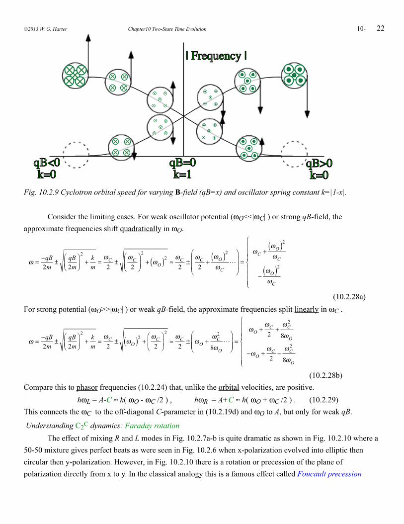
22
| Frequency |
qB>0k=0
qB=0k=1
qB<0k=0
Fig. 10.2.9 Cyclotron orbital speed for varying B-field (qB=x) and oscillator spring constant k=|1-x|.
Consider the limiting cases. For weak oscillator potential (ωO<<|ωC| ) or strong qB-field, the approximate frequencies shift quadratically in ωO.
ω = −qB2m
± qB2m
⎛⎝⎜
⎞⎠⎟
2
+ km
=ωC2
±ωC2
⎛
⎝⎜⎞
⎠⎟
2
+ ωO( )2 ≈ωC2
±ωC2
+ωO( )2ωC
⎛
⎝
⎜⎜
⎞
⎠
⎟⎟=
ωC +ωO( )2ωC
−ωO( )2ωC
⎧
⎨
⎪⎪⎪
⎩
⎪⎪⎪
(10.2.28a)For strong potential (ωO>>|ωC| ) or weak qB-field, the approximate frequencies split linearly in ωC .
ω = −qB2m
± qB2m
⎛⎝⎜
⎞⎠⎟
2
+ km
=ωC2
± ωO( )2 +ωC2
⎛
⎝⎜⎞
⎠⎟
2
≈ωC2
± ωO +ωC
2
8ωO
⎛
⎝⎜⎜
⎞
⎠⎟⎟=
ωO +ωC2
+ωC
2
8ωO
−ωO +ωC2
−ωC
2
8ωO
⎧
⎨
⎪⎪⎪
⎩
⎪⎪⎪
(10.2.28b)Compare this to phasor frequencies (10.2.24) that, unlike the orbital velocities, are positive. ωL = A-C ≈ ( ωO - ωC /2 ) , ωR = A+C ≈ ( ωO + ωC /2 ) . (10.2.29)This connects the ωC to the off-diagonal C-parameter in (10.2.19d) and ωO to A, but only for weak qB.
Understanding C2C dynamics: Faraday rotation The effect of mixing R and L modes in Fig. 10.2.7a-b is quite dramatic as shown in Fig. 10.2.10 where a 50-50 mixture gives perfect beats as were seen in Fig. 10.2.6 when x-polarization evolved into elliptic then circular then y-polarization. However, in Fig. 10.2.10 there is a rotation or precession of the plane of polarization directly from x to y. In the classical analogy this is a famous effect called Foucault precession
©2013 W. G. Harter Chapter10 Two-State Time Evolution 10-
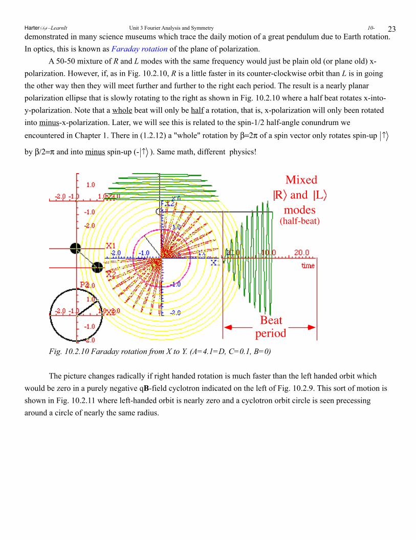
23demonstrated in many science museums which trace the daily motion of a great pendulum due to Earth rotation. In optics, this is known as Faraday rotation of the plane of polarization. A 50-50 mixture of R and L modes with the same frequency would just be plain old (or plane old) x-polarization. However, if, as in Fig. 10.2.10, R is a little faster in its counter-clockwise orbit than L is in going the other way then they will meet further and further to the right each period. The result is a nearly planar polarization ellipse that is slowly rotating to the right as shown in Fig. 10.2.10 where a half beat rotates x-into-y-polarization. Note that a whole beat will only be half a rotation, that is, x-polarization will only been rotated into minus-x-polarization. Later, we will see this is related to the spin-1/2 half-angle conundrum we encountered in Chapter 1. There in (1.2.12) a "whole" rotation by β=2π of a spin vector only rotates spin-up ↑
by β/2=π and into minus spin-up (- ↑ ). Same math, different physics!
Beatperiod
Mixed|R〉 and |L〉
modes(half-beat)
Fig. 10.2.10 Faraday rotation from X to Y. (A=4.1=D, C=0.1, B=0)
The picture changes radically if right handed rotation is much faster than the left handed orbit which would be zero in a purely negative qB-field cyclotron indicated on the left of Fig. 10.2.9. This sort of motion is shown in Fig. 10.2.11 where left-handed orbit is nearly zero and a cyclotron orbit circle is seen precessing around a circle of nearly the same radius.
HarterSoft –LearnIt Unit 3 Fourier Analysis and Symmetry 10-
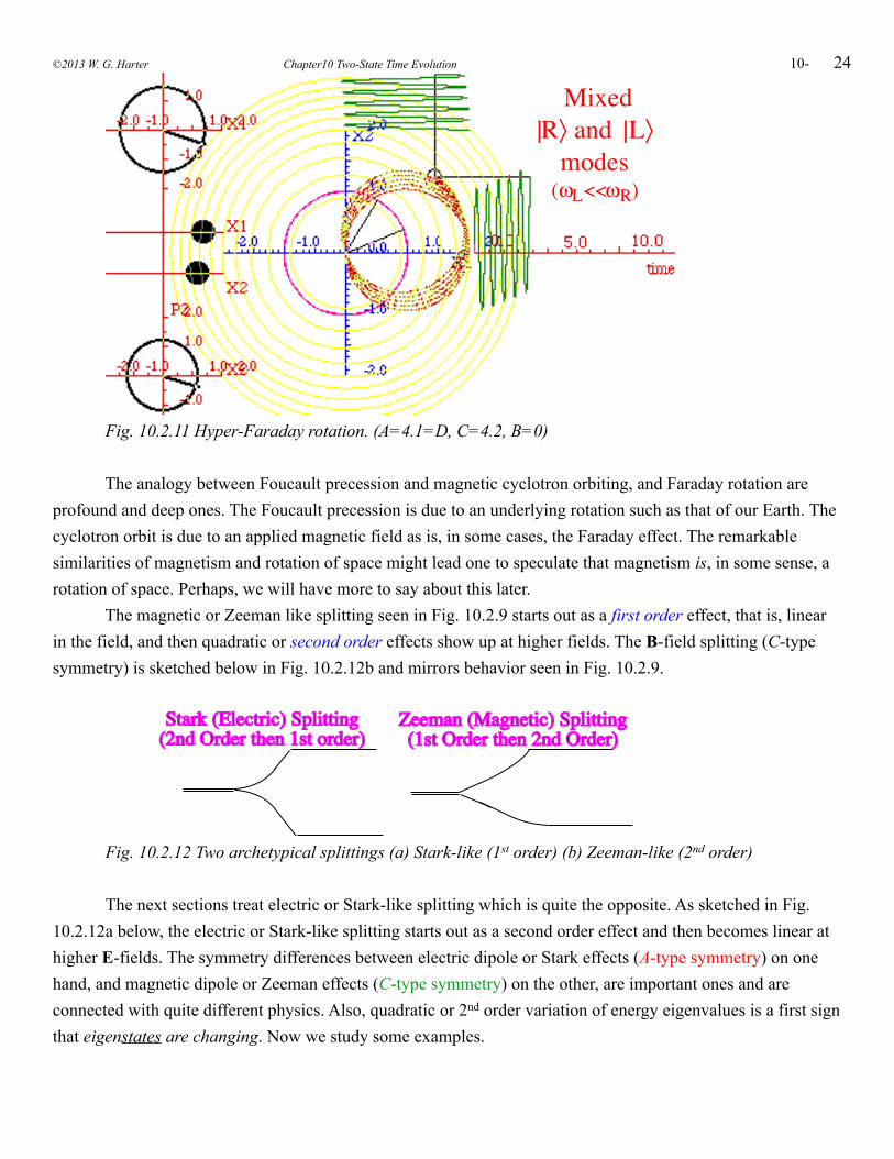
24
Mixed|R〉 and |L〉
modes(ωL<<ωR)
Fig. 10.2.11 Hyper-Faraday rotation. (A=4.1=D, C=4.2, B=0)
The analogy between Foucault precession and magnetic cyclotron orbiting, and Faraday rotation are profound and deep ones. The Foucault precession is due to an underlying rotation such as that of our Earth. The cyclotron orbit is due to an applied magnetic field as is, in some cases, the Faraday effect. The remarkable similarities of magnetism and rotation of space might lead one to speculate that magnetism is, in some sense, a rotation of space. Perhaps, we will have more to say about this later. The magnetic or Zeeman like splitting seen in Fig. 10.2.9 starts out as a first order effect, that is, linear in the field, and then quadratic or second order effects show up at higher fields. The B-field splitting (C-type symmetry) is sketched below in Fig. 10.2.12b and mirrors behavior seen in Fig. 10.2.9.
Stark (Electric) Splitting(2nd Order then 1st order)
Zeeman (Magnetic) Splitting(1st Order then 2nd Order)
Fig. 10.2.12 Two archetypical splittings (a) Stark-like (1st order) (b) Zeeman-like (2nd order)
The next sections treat electric or Stark-like splitting which is quite the opposite. As sketched in Fig. 10.2.12a below, the electric or Stark-like splitting starts out as a second order effect and then becomes linear at higher E-fields. The symmetry differences between electric dipole or Stark effects (A-type symmetry) on one hand, and magnetic dipole or Zeeman effects (C-type symmetry) on the other, are important ones and are connected with quite different physics. Also, quadratic or 2nd order variation of energy eigenvalues is a first sign that eigenstates are changing. Now we study some examples.
©2013 W. G. Harter Chapter10 Two-State Time Evolution 10-
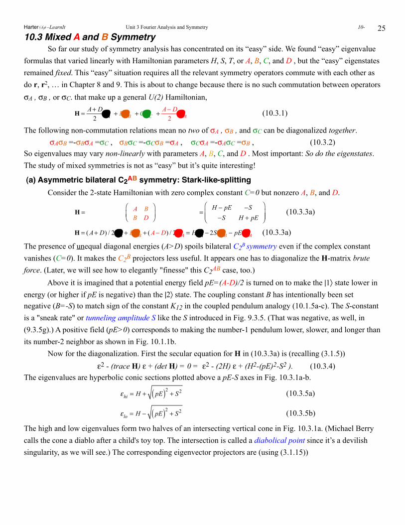
2510.3 Mixed A and B Symmetry So far our study of symmetry analysis has concentrated on its “easy” side. We found “easy” eigenvalue formulas that varied linearly with Hamiltonian parameters H, S, T, or A, B, C, and D , but the “easy” eigenstates remained fixed. This “easy” situation requires all the relevant symmetry operators commute with each other as do r, r2, … in Chapter 8 and 9. This is about to change because there is no such commutation between operators σA , σB , or σC. that make up a general U(2) Hamiltonian,
H = A+ D
2σ1 + BσB +CσC + A− D
2σ A (10.3.1)
The following non-commutation relations mean no two of σA , σB , and σC can be diagonalized together. σAσB =-σBσA =σC , σBσC =-σCσB =σA , σCσA =-σAσC =σB , (10.3.2)
So eigenvalues may vary non-linearly with parameters A, B, C, and D . Most important: So do the eigenstates. The study of mixed symmetries is not as “easy” but it’s quite interesting!
(a) Asymmetric bilateral C2AB symmetry: Stark-like-splitting Consider the 2-state Hamiltonian with zero complex constant C=0 but nonzero A, B, and D.
H = A B
B D
⎛
⎝⎜⎞
⎠⎟ =
H − pE −S−S H + pE
⎛
⎝⎜⎜
⎞
⎠⎟⎟
(10.3.3a)
H = ( A+ D) / 2 σ1 + BσB + ( A− D) / 2σ A = Hσ1 − 2S σB − pE σ A (10.3.3a)
The presence of unequal diagonal energies (A>D) spoils bilateral C2B symmetry even if the complex constant vanishes (C=0). It makes the C2B projectors less useful. It appears one has to diagonalize the H-matrix brute force. (Later, we will see how to elegantly "finesse" this C2AB case, too.) Above it is imagined that a potential energy field pE=(A-D)/2 is turned on to make the |1〉 state lower in energy (or higher if pE is negative) than the |2〉 state. The coupling constant B has intentionally been set negative (B=-S) to match sign of the constant K12 in the coupled pendulum analogy (10.1.5a-c). The S-constant is a "sneak rate" or tunneling amplitude S like the S introduced in Fig. 9.3.5. (That was negative, as well, in (9.3.5g).) A positive field (pE>0) corresponds to making the number-1 pendulum lower, slower, and longer than its number-2 neighbor as shown in Fig. 10.1.1b. Now for the diagonalization. First the secular equation for H in (10.3.3a) is (recalling (3.1.5)) ε2 - (trace H) ε + (det H) = 0 = ε2 - (2H) ε + (H2-(pE)2-S2 ). (10.3.4) The eigenvalues are hyperbolic conic sections plotted above a pE-S axes in Fig. 10.3.1a-b.
εhi = H + pE( )2 + S2 (10.3.5a)
εlo = H − pE( )2 + S2 (10.3.5b)
The high and low eigenvalues form two halves of an intersecting vertical cone in Fig. 10.3.1a. (Michael Berry calls the cone a diablo after a child's toy top. The intersection is called a diabolical point since it’s a devilish singularity, as we will see.) The corresponding eigenvector projectors are (using (3.1.15))
HarterSoft –LearnIt Unit 3 Fourier Analysis and Symmetry 10-
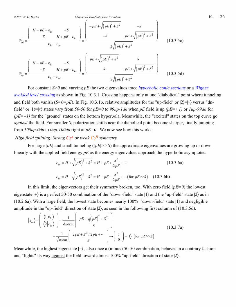
26
Phi =
H − pE − εlo −S
−S H + pE − εlo
⎛
⎝⎜⎜
⎞
⎠⎟⎟
εhi − εlo=
− pE + pE( )2 + S2 −S
−S pE + pE( )2 + S2
⎛
⎝
⎜⎜⎜⎜
⎞
⎠
⎟⎟⎟⎟
2 pE( )2 + S2 (10.3.5c)
Plo =
H − pE − εhi −S
−S H + pE − εhi
⎛
⎝⎜⎜
⎞
⎠⎟⎟
εlo − εhi=
pE + pE( )2 + S2 S
S − pE + pE( )2 + S2
⎛
⎝
⎜⎜⎜⎜
⎞
⎠
⎟⎟⎟⎟
2 pE( )2 + S2 (10.3.5d)
For constant S>0 and varying pE the two eigenvalues trace hyperbolic conic sections or a Wigner avoided level crossing as shown in Fig. 10.3.1. Crossing happens only at one "diabolical" point where tunneling and field both vanish (S=0=pE). In Fig. 10.3.1b, relative amplitudes for the "up-field" or |2〉=|y〉 versus "dn-field" or |1〉=|x〉 states vary from 50-50 for pE=0 to 99up-1dn when pE field is up (pE=+1) or 1up-99dn for (pE=−1) for the "ground" states on the bottom hyperbola. Meanwhile, the "excited" states on the top curve go against the field. For smaller S, polarization shifts near the diabolical point become sharper, finally jumping from 100up-0dn to 0up-100dn right at pE=0. We now see how this works.
High field splitting: Strong C2A or weak C2B symmetry
For large |pE| and small tunneling (|pE|>>S) the approximate eigenvalues are growing up or down linearly with the applied field energy pE as the energy eigenvalues approach the hyperbolic asymptotes.
εhi = H + pE( )2 + S2 ≈ H + pE + S2
2 pE+ (10.3.6a)
εlo = H − pE( )2 + S2 ≈ H − pE − S2
2 pE+ for: pE>>S( ) (10.3.6b)
In this limit, the eigenvectors get their symmetry broken, too. With zero field (pE=0) the lowest eigenstate |+〉 is a perfect 50-50 combination of the "down-field" state |1〉 and the "up-field" state |2〉 as in (10.2.6a). With a large field, the lowest state becomes nearly 100% "down-field" state |1〉 and negligible amplitude in the "up-field" direction of state |2〉, as seen in the following first column of (10.3.5d).
εlo =1 εlo
2 εlo
⎛
⎝⎜⎜
⎞
⎠⎟⎟= 1
norm.pE + pE( )2 + S2
S
⎛
⎝
⎜⎜
⎞
⎠
⎟⎟
≈ 1
norm.2 pE + S2 / 2 pE +
S
⎛
⎝⎜⎜
⎞
⎠⎟⎟→ 1
0
⎛
⎝⎜⎞
⎠⎟= 1 for: pE>>S( )
(10.3.7a)
Meanwhile, the highest eigenstate |−〉 , also once a (minus) 50-50 combination, behaves in a contrary fashion and "fights" its way against the field toward almost 100% "up-field" direction of state |2〉.
©2013 W. G. Harter Chapter10 Two-State Time Evolution 10-
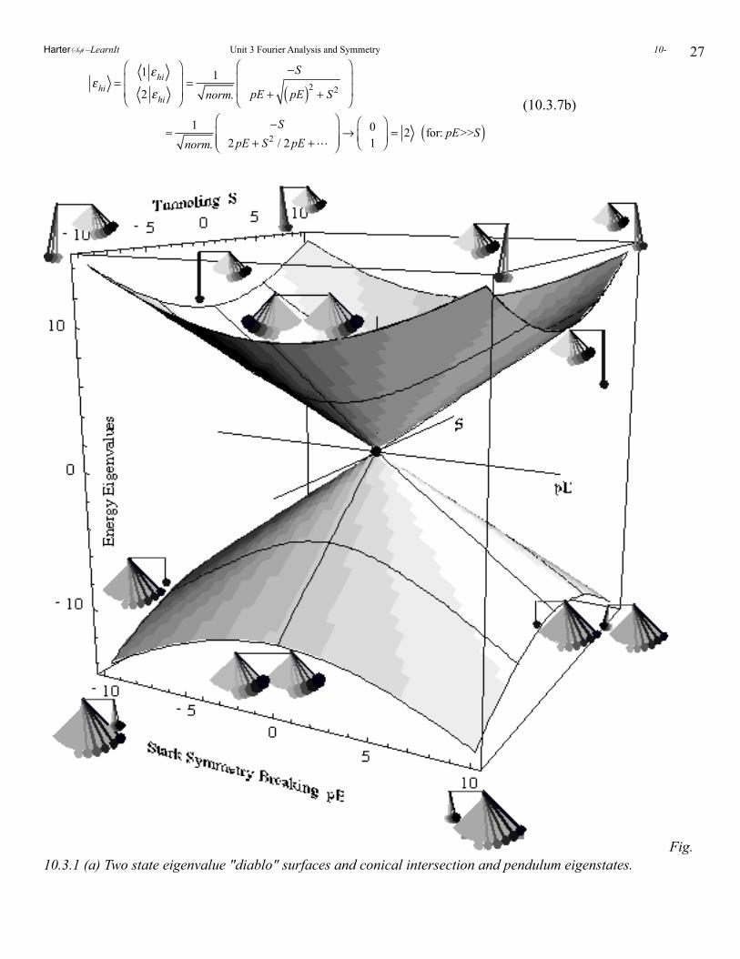
27
εhi =1 εhi
2 εhi
⎛
⎝⎜⎜
⎞
⎠⎟⎟= 1
norm.
−S
pE + pE( )2 + S2
⎛
⎝
⎜⎜
⎞
⎠
⎟⎟
≈ 1
norm.
−S
2 pE + S2 / 2 pE +
⎛
⎝⎜⎜
⎞
⎠⎟⎟→ 0
1
⎛
⎝⎜⎞
⎠⎟= 2 for: pE>>S( )
(10.3.7b)
Fig. 10.3.1 (a) Two state eigenvalue "diablo" surfaces and conical intersection and pendulum eigenstates.
HarterSoft –LearnIt Unit 3 Fourier Analysis and Symmetry 10-
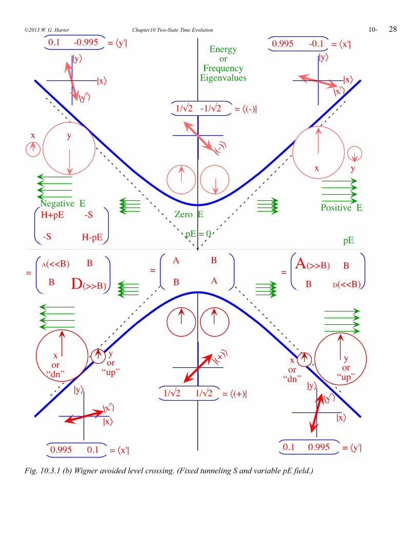
28
|x'〉|y'〉
|(+)〉
|(-)〉
|x'〉|y'〉
H+pE
H-pE
-S
-S
A(<<B)
D(>>B)
B
B=
A
A
B
B=
B=
D(<<B)
A(>>B) B
pE = 0
0.1 -0.995 = 〈y'| 0.995 -0.1 = 〈x'|
1/√2 -1/√2 = 〈(-)|
0.1 0.995 = 〈y'|0.995 0.1 = 〈x'|
1/√2 1/√2 = 〈(+)|
Energyor
FrequencyEigenvalues
pE
Positive ENegative EZero E
yor“up”
|x〉
|y〉
xor“dn”
|x〉
|y〉
|x〉
|y〉
|x〉
|y〉
yor“up”
xor“dn”
yx
yx
Fig. 10.3.1 (b) Wigner avoided level crossing. (Fixed tunneling S and variable pE field.)
©2013 W. G. Harter Chapter10 Two-State Time Evolution 10-
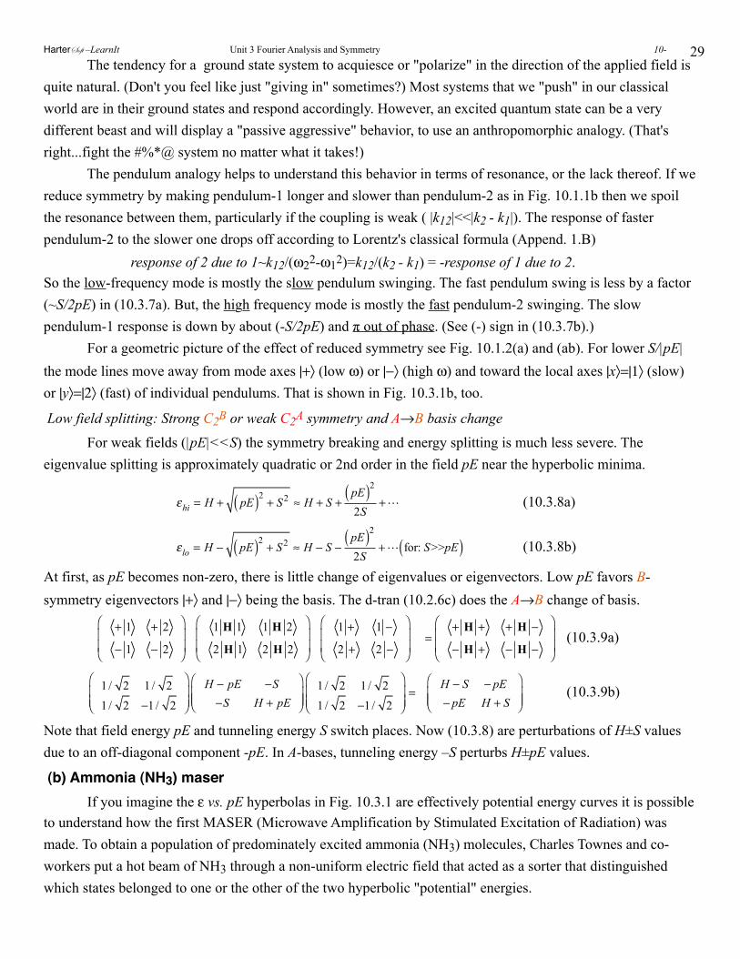
29 The tendency for a ground state system to acquiesce or "polarize" in the direction of the applied field is quite natural. (Don't you feel like just "giving in" sometimes?) Most systems that we "push" in our classical world are in their ground states and respond accordingly. However, an excited quantum state can be a very different beast and will display a "passive aggressive" behavior, to use an anthropomorphic analogy. (That's right...fight the #%*@ system no matter what it takes!) The pendulum analogy helps to understand this behavior in terms of resonance, or the lack thereof. If we reduce symmetry by making pendulum-1 longer and slower than pendulum-2 as in Fig. 10.1.1b then we spoil the resonance between them, particularly if the coupling is weak ( |k12|<<|k2 - k1|). The response of faster pendulum-2 to the slower one drops off according to Lorentz's classical formula (Append. 1.B) response of 2 due to 1~k12/(ω22-ω12)=k12/(k2 - k1) = -response of 1 due to 2. So the low-frequency mode is mostly the slow pendulum swinging. The fast pendulum swing is less by a factor (~S/2pE) in (10.3.7a). But, the high frequency mode is mostly the fast pendulum-2 swinging. The slow pendulum-1 response is down by about (-S/2pE) and π out of phase. (See (-) sign in (10.3.7b).) For a geometric picture of the effect of reduced symmetry see Fig. 10.1.2(a) and (ab). For lower S/|pE| the mode lines move away from mode axes |+〉 (low ω) or |−〉 (high ω) and toward the local axes |x〉=|1〉 (slow) or |y〉=|2〉 (fast) of individual pendulums. That is shown in Fig. 10.3.1b, too.
Low field splitting: Strong C2B or weak C2A symmetry and A→B basis change
For weak fields (|pE|<<S) the symmetry breaking and energy splitting is much less severe. The eigenvalue splitting is approximately quadratic or 2nd order in the field pE near the hyperbolic minima.
εhi = H + pE( )2 + S2 ≈ H + S +
pE( )22S
+ (10.3.8a)
εlo = H − pE( )2 + S2 ≈ H − S −
pE( )22S
+ for: S>>pE( ) (10.3.8b)
At first, as pE becomes non-zero, there is little change of eigenvalues or eigenvectors. Low pE favors B-symmetry eigenvectors |+〉 and |−〉 being the basis. The d-tran (10.2.6c) does the A→B change of basis.
+ 1 + 2
− 1 − 2
⎛
⎝⎜⎜
⎞
⎠⎟⎟
1 H 1 1 H 2
2 H 1 2 H 2
⎛
⎝⎜⎜
⎞
⎠⎟⎟
1 + 1 −
2 + 2 −
⎛
⎝⎜⎜
⎞
⎠⎟⎟
=+ H + + H −
− H + − H −
⎛
⎝⎜⎜
⎞
⎠⎟⎟
(10.3.9a)
1 / 2 1 / 21 / 2 −1 / 2
⎛
⎝⎜⎜
⎞
⎠⎟⎟
H − pE −S−S H + pE
⎛
⎝⎜⎜
⎞
⎠⎟⎟
1 / 2 1 / 21 / 2 −1 / 2
⎛
⎝⎜⎜
⎞
⎠⎟⎟=
H − S − pE− pE H + S
⎛
⎝⎜⎜
⎞
⎠⎟⎟
(10.3.9b)
Note that field energy pE and tunneling energy S switch places. Now (10.3.8) are perturbations of H±S values due to an off-diagonal component -pE. In A-bases, tunneling energy –S perturbs H±pE values.
(b) Ammonia (NH3) maser If you imagine the ε vs. pE hyperbolas in Fig. 10.3.1 are effectively potential energy curves it is possible to understand how the first MASER (Microwave Amplification by Stimulated Excitation of Radiation) was made. To obtain a population of predominately excited ammonia (NH3) molecules, Charles Townes and co-workers put a hot beam of NH3 through a non-uniform electric field that acted as a sorter that distinguished which states belonged to one or the other of the two hyperbolic "potential" energies.
HarterSoft –LearnIt Unit 3 Fourier Analysis and Symmetry 10-
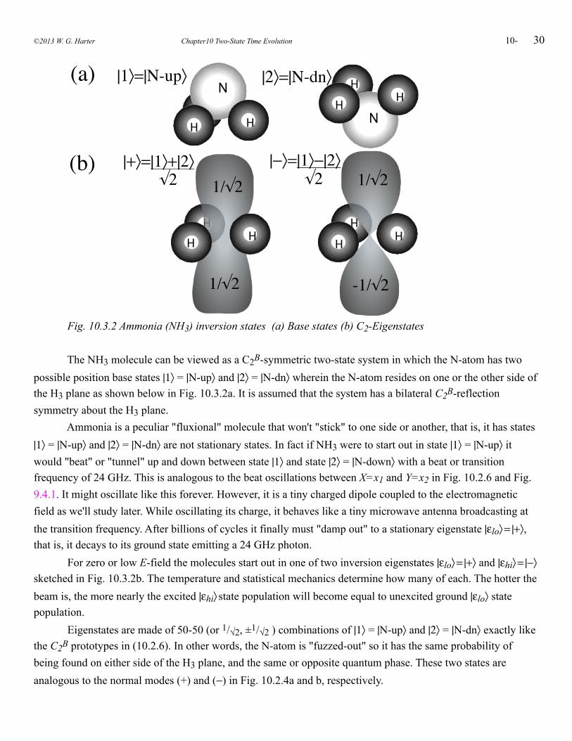
30
H
N|1〉=|N-up〉 H
N
|2〉=|N-dn〉H H
HH
(a)
H H H H
|+〉=|1〉+|2〉√2 1/√2
1/√2 -1/√2
1/√2|−〉=|1〉−|2〉
√2(b)
Fig. 10.3.2 Ammonia (NH3) inversion states (a) Base states (b) C2-Eigenstates
The NH3 molecule can be viewed as a C2B-symmetric two-state system in which the N-atom has two possible position base states |1〉 = |N-up〉 and |2〉 = |N-dn〉 wherein the N-atom resides on one or the other side of the H3 plane as shown below in Fig. 10.3.2a. It is assumed that the system has a bilateral C2B-reflection symmetry about the H3 plane. Ammonia is a peculiar "fluxional" molecule that won't "stick" to one side or another, that is, it has states |1〉 = |N-up〉 and |2〉 = |N-dn〉 are not stationary states. In fact if NH3 were to start out in state |1〉 = |N-up〉 it would "beat" or "tunnel" up and down between state |1〉 and state |2〉 = |N-down〉 with a beat or transition frequency of 24 GHz. This is analogous to the beat oscillations between X=x1 and Y=x2 in Fig. 10.2.6 and Fig. 9.4.1. It might oscillate like this forever. However, it is a tiny charged dipole coupled to the electromagnetic field as we'll study later. While oscillating its charge, it behaves like a tiny microwave antenna broadcasting at the transition frequency. After billions of cycles it finally must "damp out" to a stationary eigenstate |εlo〉 = |+〉, that is, it decays to its ground state emitting a 24 GHz photon. For zero or low E-field the molecules start out in one of two inversion eigenstates |εlo〉 = |+〉 and |εhi〉 = |−〉 sketched in Fig. 10.3.2b. The temperature and statistical mechanics determine how many of each. The hotter the beam is, the more nearly the excited |εhi〉 state population will become equal to unexcited ground |εlo〉 state population. Eigenstates are made of 50-50 (or 1/√2, ±1/√2 ) combinations of |1〉 = |N-up〉 and |2〉 = |N-dn〉 exactly like the C2B prototypes in (10.2.6). In other words, the N-atom is "fuzzed-out" so it has the same probability of being found on either side of the H3 plane, and the same or opposite quantum phase. These two states are analogous to the normal modes (+) and (−) in Fig. 10.2.4a and b, respectively.
©2013 W. G. Harter Chapter10 Two-State Time Evolution 10-
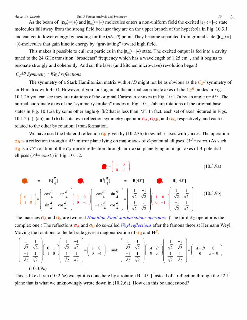
31 As the beam of |εlo〉 = |+〉 and |εhi〉 = |−〉 molecules enters a non-uniform field the excited |εhi〉 = |−〉 state molecules fall away from the strong field because they are on the upper branch of the hyperbola in Fig. 10.3.1 and can get to lower energy by heading for the (pE=0) point. They become separated from ground state (|εlo〉 = |+〉)-molecules that gain kinetic energy by “gravitating” toward high field. This makes it possible to cull out particles in the |εhi〉 = |−〉 state. The excited output is fed into a cavity tuned to the 24 GHz transition "broadcast" frequency which has a wavelength of 1.25 cm. , and it begins to resonate strongly and coherently. And so, the laser (and kitchen microwave) revolution began!
C2AB Symmetry : Weyl reflections
The symmetry of a Stark Hamiltonian matrix with A≠D might not be as obvious as the C2B symmetry of an H-matrix with A=D. However, if you look again at the normal coordinate axes of the C2B modes in Fig. 10.1.2b you can see they are rotations of the original Cartesian xy-axes in Fig. 10.1.2a by an angle φ=45°. The normal coordinate axes of the "symmetry-broken" modes in Fig. 10.1.2ab are rotations of the original base states in Fig. 10.1.2a by some other angle φ=β/2 that is less than 45°. In fact, each set of axes pictured in Figs. 10.1.2 (a), (ab), and (b) has its own reflection symmetry operator σΑ, σΑΒ, and σΒ, respectively, and each is related to the other by rotational transformation. We have used the bilateral reflection σΒ given by (10.2.3b) to switch x-axes with y-axes. The operation σΒ is a reflection through a 45° mirror plane lying on major axes of B-potential ellipses. (VB=const.) As such, σΒ is a 45° rotation of the σΑ mirror reflection through an x-axial plane lying on major axes of A-potential ellipses (VA=const.) in Fig. 10.1.2.
σ A = 1 0
0 −1⎛
⎝⎜⎞
⎠⎟ (10.3.9a)
σB = R[π4
] σ A R†[π4
] = R[45°] σ A R[−45°]
0 11 0
⎛
⎝⎜⎞
⎠⎟=
cosπ4
−sinπ4
sinπ4
cosπ4
⎛
⎝
⎜⎜⎜⎜
⎞
⎠
⎟⎟⎟⎟
1 00 −1
⎛
⎝⎜⎞
⎠⎟cos
π4
sinπ4
−sinπ4
cosπ4
⎛
⎝
⎜⎜⎜⎜
⎞
⎠
⎟⎟⎟⎟
=
1
2
−1
21
2
1
2
⎛
⎝
⎜⎜⎜⎜⎜
⎞
⎠
⎟⎟⎟⎟⎟
1 00 −1
⎛
⎝⎜⎞
⎠⎟
1
2
1
2−1
2
1
2
⎛
⎝
⎜⎜⎜⎜⎜
⎞
⎠
⎟⎟⎟⎟⎟
(10.3.9b)
The matrices σΑ and σΒ are two real Hamilton-Pauli-Jordan spinor operators. (The third σC operator is the complex one.) The reflections σΑ and σΒ do so-called Weyl reflections after the famous theorist Hermann Weyl. Moving the rotations to the left side gives a diagonalization of σΒ and HB.
12
12
−12
12
⎛
⎝
⎜⎜⎜⎜⎜
⎞
⎠
⎟⎟⎟⎟⎟
0 11 0
⎛
⎝⎜⎞
⎠⎟
12
−12
12
12
⎛
⎝
⎜⎜⎜⎜⎜
⎞
⎠
⎟⎟⎟⎟⎟
= 1 00 −1
⎛
⎝⎜⎞
⎠⎟ , and:
12
12
−12
12
⎛
⎝
⎜⎜⎜⎜⎜
⎞
⎠
⎟⎟⎟⎟⎟
A BB A
⎛
⎝⎜⎞
⎠⎟
12
−12
12
12
⎛
⎝
⎜⎜⎜⎜⎜
⎞
⎠
⎟⎟⎟⎟⎟
= A+ B 00 A− B
⎛
⎝⎜⎞
⎠⎟
(10.3.9c)This is like d-tran (10.2.6c) except it is done here by a rotation R[-45°] instead of a reflection through the 22.5° plane that is what we unknowingly wrote down in (10.2.6a). How can this be understood?
HarterSoft –LearnIt Unit 3 Fourier Analysis and Symmetry 10-
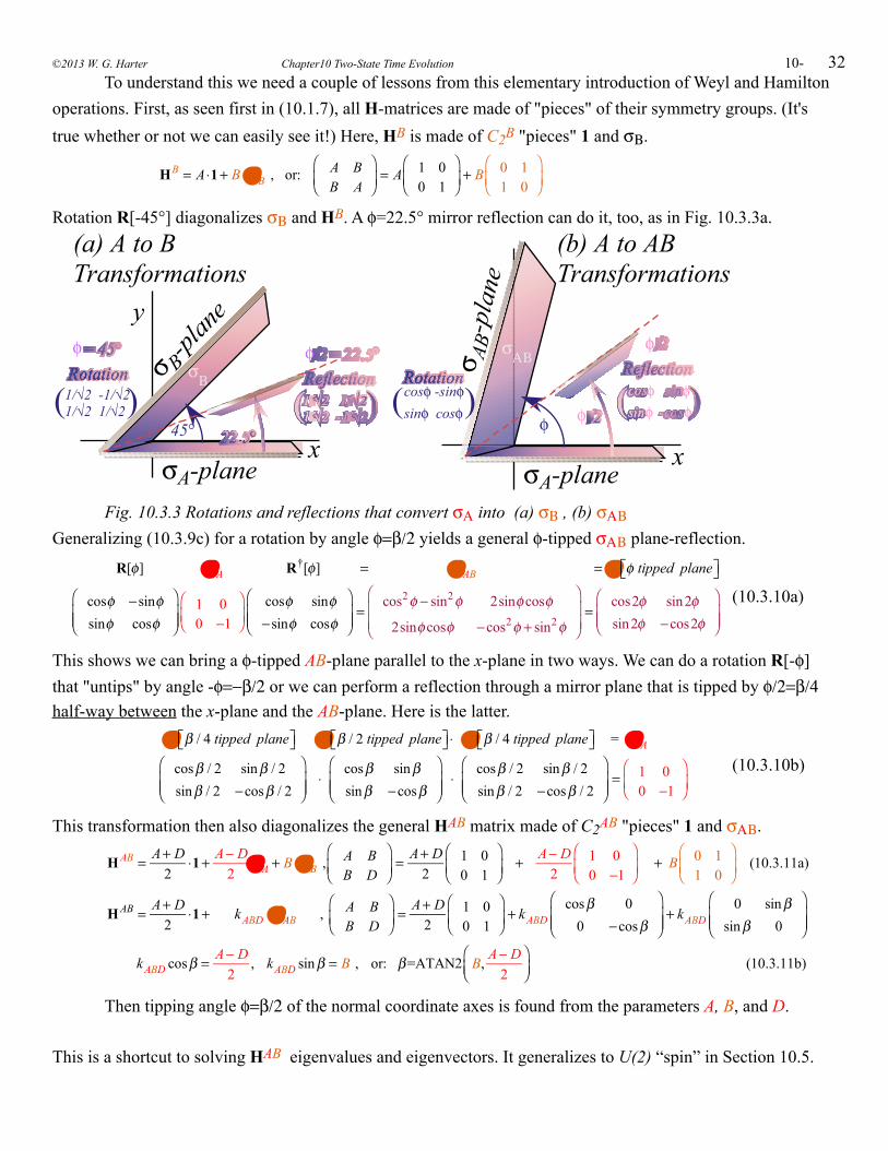
32 To understand this we need a couple of lessons from this elementary introduction of Weyl and Hamilton operations. First, as seen first in (10.1.7), all H-matrices are made of "pieces" of their symmetry groups. (It's true whether or not we can easily see it!) Here, HB is made of C2B "pieces" 1 and σΒ.
HB = A ⋅1+ B ⋅ σB , or: A B
B A⎛
⎝⎜⎞
⎠⎟= A 1 0
0 1
⎛
⎝⎜⎞
⎠⎟+ B 0 1
1 0
⎛
⎝⎜⎞
⎠⎟
Rotation R[-45°] diagonalizes σΒ and HB. A φ=22.5° mirror reflection can do it, too, as in Fig. 10.3.3a.
45°
σ B-plane
σΒ
σA-planex
y
1/√2 -1/√21/√2 1/√2( )
(a) A to BTransformations
σ AB-plane
φ
σΑΒ
σA-planex
cosφ -sinφsinφ cosφ( )
(b) A to ABTransformations
φ φ φ
φφφ
φφ
Fig. 10.3.3 Rotations and reflections that convert σΑ into (a) σΒ , (b) σΑΒ Generalizing (10.3.9c) for a rotation by angle φ=β/2 yields a general φ-tipped σΑΒ plane-reflection.
R[φ] σ A R†[φ] = σ AB = σ φ tipped plane⎡⎣ ⎤⎦
cosφ −sinφsinφ cosφ
⎛
⎝⎜⎜
⎞
⎠⎟⎟
1 00 −1
⎛
⎝⎜⎞
⎠⎟cosφ sinφ−sinφ cosφ
⎛
⎝⎜⎜
⎞
⎠⎟⎟=
cos2φ − sin2φ 2sinφ cosφ
2sinφ cosφ −cos2φ + sin2φ
⎛
⎝⎜⎜
⎞
⎠⎟⎟=
cos2φ sin2φsin2φ −cos2φ
⎛
⎝⎜⎜
⎞
⎠⎟⎟
(10.3.10a)
This shows we can bring a φ-tipped AB-plane parallel to the x-plane in two ways. We can do a rotation R[-φ] that "untips" by angle -φ=−β/2 or we can perform a reflection through a mirror plane that is tipped by φ/2=β/4 half-way between the x-plane and the AB-plane. Here is the latter.
σ β / 4 tipped plane⎡⎣ ⎤⎦ ⋅ σ β / 2 tipped plane⎡⎣ ⎤⎦ ⋅ σ β / 4 tipped plane⎡⎣ ⎤⎦ = σ A
cosβ / 2 sinβ / 2sinβ / 2 −cosβ / 2
⎛
⎝⎜⎜
⎞
⎠⎟⎟
⋅ cosβ sinβsinβ −cosβ
⎛
⎝⎜⎜
⎞
⎠⎟⎟
⋅ cosβ / 2 sinβ / 2sinβ / 2 −cosβ / 2
⎛
⎝⎜⎜
⎞
⎠⎟⎟= 1 0
0 −1
⎛
⎝⎜⎞
⎠⎟ (10.3.10b)
This transformation then also diagonalizes the general HAB matrix made of C2AB "pieces" 1 and σΑΒ.
H AB = A+ D2
⋅1+ A− D2
σ A + B ⋅ σB , A BB D
⎛
⎝⎜⎞
⎠⎟= A+ D
21 00 1
⎛
⎝⎜⎞
⎠⎟ +
A− D2
1 00 −1
⎛
⎝⎜⎞
⎠⎟ + B 0 1
1 0
⎛
⎝⎜⎞
⎠⎟ (10.3.11a)
H AB = A+ D2
⋅1+ kABD ⋅ σ AB , A BB D
⎛
⎝⎜⎞
⎠⎟= A+ D
21 00 1
⎛
⎝⎜⎞
⎠⎟+ kABD
cosβ 00 −cosβ
⎛
⎝⎜⎜
⎞
⎠⎟⎟+ kABD
0 sinβsinβ 0
⎛
⎝⎜⎜
⎞
⎠⎟⎟
kABD cosβ = A− D2
, kABD sinβ = B , or: β=ATAN2 B,A− D
2⎛⎝⎜
⎞⎠⎟
(10.3.11b)
Then tipping angle φ=β/2 of the normal coordinate axes is found from the parameters A, B, and D.
This is a shortcut to solving HAB eigenvalues and eigenvectors. It generalizes to U(2) “spin” in Section 10.5.
©2013 W. G. Harter Chapter10 Two-State Time Evolution 10-
33Unitary U(2) versus Special Unitary SU(2) Before continuing, we should elaborate on some fine points and terminology. In Sec. 2.2 (d) and (e) we introduced the unitary group U(n) of operators U that satisfy unitarity (U†U=1) and its subgroup called the special unitary group SU(n) which had an additional requirement of unimodularity. (det|U|=1 )Note that rotational operators like R[-45°] belong to SU(2) while reflection operators like σΑΒ belong to U(2) (σ†σ=σσ=1) but not SU(2) because σ's have (-1) determinants. ( det|σ|=-1) Mirror reflections change left handed gloves into right handed ones. Since two reflections through the same mirror is an identity operation (σσ=1) it follows that reflections are both Hermitian (σ†=σ) and unitary (σ†σ=1). In some sense they are the most “perfectly normal” operators. If you multiply two members of SU(2) the product has to be an SU(2) member, too. (Closure axiom) So, products of rotations can never yield a reflection. However, the product of two reflections will have a positive unit determinant, in fact, it will be a rotation. This is easily see by an example that multiplies x-plane reflection σΑ in (10.2.13a) by an AB-plane or φ-tipped reflection σΑΒ in (10.2.14a) .
σ φ tipped plane⎡⎣ ⎤⎦ · σ A = R 2φ⎡⎣ ⎤⎦ , or: σ A · σ φ tipped plane⎡⎣ ⎤⎦ = R −2φ⎡⎣ ⎤⎦
cos2φ sin2φsin2φ −cos2φ
⎛
⎝⎜⎜
⎞
⎠⎟⎟
1 00 −1
⎛
⎝⎜⎞
⎠⎟=
cos2φ −sin2φsin2φ cos2φ
⎛
⎝⎜⎜
⎞
⎠⎟⎟
, or: 1 00 −1
⎛
⎝⎜⎞
⎠⎟cos2φ sin2φsin2φ −cos2φ
⎛
⎝⎜⎜
⎞
⎠⎟⎟=
cos2φ sin2φ−sin2φ cos2φ
⎛
⎝⎜⎜
⎞
⎠⎟⎟
(10.3.12)
In other words, rotations are composed of reflections, and not vice-versa. The σ's are more fundamental than the R's. In some sense reflections are "square roots" of rotations. One only needs half the angle φ=β/2 to do the job that a full angle 2φ=β rotation would need. As seen in (10.3.10) a pair of mirror planes separated by angle φ=β/2 will perform a rotation by either β or -β , depending on the order of action.
Complete sets of commuting operators One may turn the discussion of symmetry inside-out by asking what are all the operators Q that commute with a given H-matrix (or set of commuting H-matrices). Spectral decomposition gives the answers to such questions, for if Pk are the irreducible projectors of H (or set of H's) then the answer is Q = Σ αk Pk (= α1 P1 + α2 P2 , for 2-by-2 Q) (10.3.13a)for arbitrary complex numbers αk . If you further restrict Q to be unitary (in U(n)) then the answer is Q = Σ eiαk Pk (= eiα1 P1 + eiα2 P2 , for 2-by-2 Q) (10.3.13b)for arbitrary real numbers αk . Finally, if you want Q to be unimodular (in SU(n)), too, then the answer is Q = Σ eiαk Pk (= e-iαP1 + eiαP2 for 2-by-2 Q) (10.3.13c)where angles in exponents must sum to zero or multiples of 2π. (Σαk = 2πn) For example, the SU(2) symmetry operators that commute with HB must be of the form
Q = e−iχ
21 11 1
⎛
⎝⎜⎞
⎠⎟+ eiχ
21 −1−1 1
⎛
⎝⎜⎞
⎠⎟=
cosχ −isinχ−isinχ cosχ
⎛
⎝⎜⎜
⎞
⎠⎟⎟= R B χ( ) (10.3.14)
In other words, the only rotations that commute with HB are imaginary or complex. It turns out these are representations of Lorentz transformations that provide a relativistic theory of polarization.
HarterSoft –LearnIt Unit 3 Fourier Analysis and Symmetry 10-
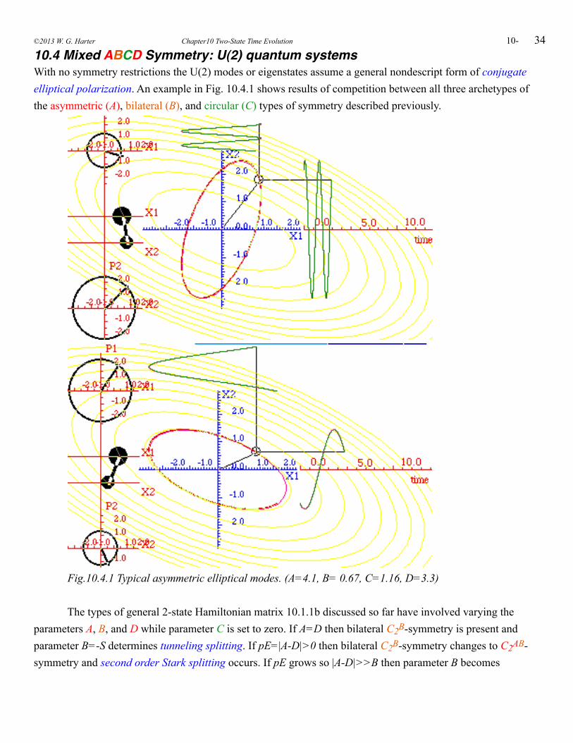
3410.4 Mixed ABCD Symmetry: U(2) quantum systemsWith no symmetry restrictions the U(2) modes or eigenstates assume a general nondescript form of conjugate elliptical polarization. An example in Fig. 10.4.1 shows results of competition between all three archetypes of the asymmetric (A), bilateral (B), and circular (C) types of symmetry described previously.
Fig.10.4.1 Typical asymmetric elliptical modes. (A=4.1, B= 0.67, C=1.16, D=3.3)
The types of general 2-state Hamiltonian matrix 10.1.1b discussed so far have involved varying the parameters A, B, and D while parameter C is set to zero. If A=D then bilateral C2B-symmetry is present and parameter B=-S determines tunneling splitting. If pE=|A-D|>0 then bilateral C2B-symmetry changes to C2AB-symmetry and second order Stark splitting occurs. If pE grows so |A-D|>>B then parameter B becomes
©2013 W. G. Harter Chapter10 Two-State Time Evolution 10-
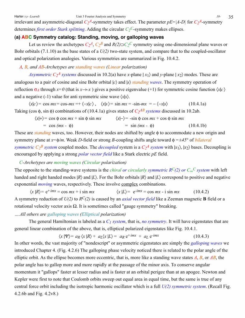
35irrelevant and asymmetric-diagonal C2A-symmetry takes effect. The parameter pE=|A-D| for C2A-symmetry determines first order Stark splitting. Adding the circular C2C-symmetry makes ellipses.
(a) ABC Symmetry catalog: Standing, moving, or galloping waves Let us review the archetypes C2A, C2B and R(2)⊃C2C symmetry using one-dimensional plane waves or Bohr orbitals (7.1.10) as the base states of a U(2) two-state system, and compare that to the coupled-oscillator and optical polarization analogies. Various symmetries are summarized in Fig. 10.4.2.
A, B, and AB-Archetypes are standing waves (Linear polarization) Asymmetric C2A systems discussed in 10.2(a) have x-plane | x1〉 and y-plane | x2〉 modes. These are analogous to a pair of cosine and sine Bohr orbital |c〉 and |s〉 standing waves. The symmetry operation of reflection σA through x=0 (that is x→-x ) gives a positive eigenvalue (+1) for symmetric cosine function 〈x|c 〉 and a negative (-1) value for anti symmetric sine wave 〈x|s〉. 〈x|c 〉 = cos mx = cos-mx =+ 〈−x|c 〉 , 〈x|s 〉 = sin mx = -sin-mx = − 〈−x|s〉 (10.4.1a)Taking (cos φ, sin φ) combinations of (10.4.1a) gives states of C2AB systems discussed in 10.2ab. 〈x|+〉 = cos φ cos mx + sin φ sin mx 〈x|−〉 = -sin φ cos mx + cos φ sin mx = cos (mx - φ) = sin (mx - φ) (10.4.1b)These are standing waves, too. However, their nodes are shifted by angle φ to accommodate a new origin and symmetry plane at x=φ/m. Weak D-field or strong B-coupling shifts angle toward φ =±45° of bilateral symmetric C2B system coupled modes. The decoupled system is a C2A system with |x1〉, |x2〉 bases. Decoupling is encouraged by applying a strong polar vector field like a Stark electric pE field.
C-Archetypes are moving waves (Circular polarization)The opposite to the standing-wave systems is the chiral or circularly symmetric RC(2) or C∞C system with left handed and right handed modes |R〉 and |L〉. For the Bohr orbitals |R〉 and |L〉 correspond to positive and negative exponential moving waves, respectively. These involve complex combinations. 〈x |R〉 = e+imx = cos mx + i sin mx 〈x |L〉 = e-imx = cos mx - i sin mx (10.4.2)A symmetry reduction of U(2) to RC(2) is caused by an axial vector field like a Zeeman magnetic B field or a rotational velocity vector axis Ω. It is sometimes called "gauge symmetry" breaking.
….All others are galloping waves (Elliptical polarization) The general Hamiltonian is labeled as a C1 system, that is, no symmetry. It will have eigenstates that are general linear combination of the above, that is, elliptical polarized eigenstates like Fig. 10.4.1. 〈x |Ψ〉 = aR 〈x |R〉 + aL〈x |L〉 = aR e+imx + aL e-imx (10.4.3)In other words, the vast majority of "nondescript" or asymmetric eigenstates are simply the galloping waves we introduced Chapter 4. (Fig. 4.2.6) The galloping phase velocity noticed there is related to the polar angle of the elliptic orbit. As the ellipse becomes more eccentric, that is, more like a standing wave states A, B, or AB, the polar angle has to gallop more and more rapidly at the passage of the minor axis. To conserve angular momentum it "gallops" faster at lesser radius and is faster at an orbital perigee than at an apogee. Newton and Kepler were first to note that Coulomb orbits sweep out equal area in equal time, but the same is true of any central force orbit including the isotropic harmonic oscillator which is a full U(2) symmetric system. (Recall Fig. 4.2.6b and Fig. 4.2v8.)
HarterSoft –LearnIt Unit 3 Fourier Analysis and Symmetry 10-
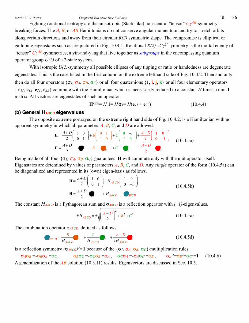
36Fighting rotational isotropy are the anisotropic (Stark-like) non-central "tensor" C2AB-symmetry-
breaking forces. The A, B, or AB Hamiltonians do not conserve angular momentum and try to stretch orbits along certain directions and away from their circular R(2) symmetric shape. The compromise is elliptical or galloping eigenstates such as are pictured in Fig. 10.4.1. Rotational R(2)⊃C2C symmetry is the mortal enemy of “tensor” C2AB-symmetries, a yin-and-yang that live together as subgroups in the encompassing quantum operator group U(2) of a 2-state system.
With isotropic U(2)-symmetry all possible ellipses of any tipping or ratio or handedness are degenerate eigenstates. This is the case listed in the first column on the extreme lefthand side of Fig. 10.4.2. Then and only then do all four operators {σ1, σA, σB, σC} or all four quaternions {1, i, j, k} or all four elementary operators { e11, e12, e21, e22} commute with the Hamiltonian which is necessarily reduced to a constant H times a unit-1 matrix. All vectors are eigenstates of such an operator.
HU(2)= H 1= H σ1= H(e11 + e22) (10.4.4)
(b) General HABCD eigenvalues The opposite extreme portrayed on the extreme right hand side of Fig. 10.4.2, is a Hamiltonian with no apparent symmetry in which all parameters A, B, C, and D are allowed.
H = A+ D2
1 00 1
⎛
⎝⎜⎞
⎠⎟+ B 0 1
1 0⎛
⎝⎜⎞
⎠⎟+C 0 −i
i 0⎛
⎝⎜⎞
⎠⎟+ A− D
21 00 −1
⎛
⎝⎜⎞
⎠⎟
H = A+ D2
σ1 + B σB +C σC + A− D2
σ A
(10.4.5a)
Being made of all four {σ1, σA, σB, σC} guarantees H will commute only with the unit operator itself. Eigenstates are detemined by values of parameters A, B, C, and D. Any single operator of the form (10.4.5a) can be diagonalized and represented in its (own) eigen-basis as follows.
H = A+ D2
1 00 1
⎛
⎝⎜⎞
⎠⎟+ H ABCD
1 00 −1
⎛
⎝⎜⎞
⎠⎟
H = A+ D2
σ1 + H ABCD σ ABCD
(10.4.5b)
The constant HABCD is a Pythagorean sum and σABCD is a reflection operator with (±1)-eigenvalues.
±H ABCD = ± A− D
2⎛⎝⎜
⎞⎠⎟
2
+ B2 +C2 (10.4.5c)
The combination operator σABCD defined as follows
σ ABCD = B
H ABCDσB + C
H ABCD σC + A− D
2H ABCDσ A (10.4.5d)
is a reflection symmetry (σABCD)2=1 because of the {σ1, σA, σB, σC}-multiplication rules. σAσB =-σBσA =σC , σBσC =-σCσB =σA , σCσA =-σAσC =σB , σA 2=σB2=σC2=1 (10.4.6)A generalization of the AB solution (10.3.11) results. Eigenvectors are discussed in Sec. 10.5.
©2013 W. G. Harter Chapter10 Two-State Time Evolution 10-
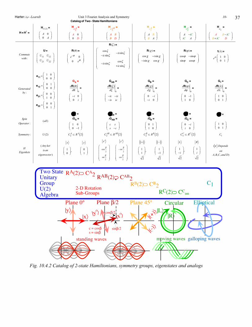
37
Catalog of Two -State Hamiltonians
H = H† =HU (2) =
A 00 A
⎛
⎝⎜⎞
⎠⎟
HC2
A =
A 00 D
⎛
⎝⎜⎞
⎠⎟
HC2
AB =
A BB D
⎛
⎝⎜⎞
⎠⎟
HC2
B =
A BB A
⎛
⎝⎜⎞
⎠⎟
HC2
C =
A −iCiC A
⎛
⎝⎜⎞
⎠⎟
HC1
=
A B − iCB + iC D
⎛
⎝⎜⎞
⎠⎟
Commutewith :
U =U11 U12
U21 U22
⎛
⎝⎜⎜
⎞
⎠⎟⎟
R(θ ) =
e−iθ 0
0 eiθ
⎛
⎝⎜⎜
⎞
⎠⎟⎟
R(ζ ) =
cosζ−icsinζ
−issinζ
−issinζcosζ
+icsinζ
⎛
⎝
⎜⎜⎜⎜⎜⎜
⎞
⎠
⎟⎟⎟⎟⎟⎟
R(χ ) =
cosχ −isinχ−isinχ cosχ
⎛
⎝⎜⎜
⎞
⎠⎟⎟
R(ϕ ) =
cosϕ −sinϕsinϕ cosϕ
⎛
⎝⎜⎜
⎞
⎠⎟⎟
1(λ) =
eiλ 1 00 1
⎛
⎝⎜⎞
⎠⎟
Generatedby :
e11 =1 00 0
⎛
⎝⎜⎞
⎠⎟
e12 = 0 10 0
⎛
⎝⎜⎞
⎠⎟
e21 =0 01 0
⎛
⎝⎜⎞
⎠⎟
e22 = 0 00 1
⎛
⎝⎜⎞
⎠⎟
GA =dR(θ )
dθ 0=
−i 00 i
⎛
⎝⎜⎞
⎠⎟
GAB =dR(ζ )
dζ 0=
−ic −is−is ic
⎛
⎝⎜⎞
⎠⎟
GB =dR(χ )
dχ 0=
0 −i−i 0
⎛
⎝⎜⎞
⎠⎟
GC =dR(ϕ )
dϕ 0=
0 −11 0
⎛
⎝⎜⎞
⎠⎟
G1 =dR(λ)
dλ 0=
1 00 1
⎛
⎝⎜⎞
⎠⎟
SpinOperator :
(all)
σA =iGA =
1 00 −1
⎛
⎝⎜⎞
⎠⎟
σAB =iGAB =
c ss −c
⎛
⎝⎜⎞
⎠⎟
σB =iGB =
0 11 0
⎛
⎝⎜⎞
⎠⎟
σC =iGC =
0 −ii 0
⎛
⎝⎜⎞
⎠⎟
σ0 =
1 00 1
⎛
⎝⎜⎞
⎠⎟
Symmetry : U (2) C2A ⊂ R A 2( ) C2
AB ⊂ R AB 2( ) C2B ⊂ RB 2( ) C∞
C ⊂ RC 2( ) C1
HEigenkets
( Any ketisan
eigenvector)
x
10
⎛
⎝⎜⎞
⎠⎟,
y
01
⎛
⎝⎜⎞
⎠⎟
x '
cosβ
2
sinβ
2
⎛
⎝
⎜⎜⎜⎜
⎞
⎠
⎟⎟⎟⎟
y '
− sinβ
2
cosβ
2
⎛
⎝
⎜⎜⎜⎜
⎞
⎠
⎟⎟⎟⎟
+( )11
⎛
⎝⎜⎞
⎠⎟,
2
−( )1−1
⎛
⎝⎜⎞
⎠⎟
2
L
1−i
⎛
⎝⎜⎞
⎠⎟,
2
R
1i
⎛
⎝⎜⎞
⎠⎟
2
( ε Depends
onA, B,C,and D)
|x〉|y〉
|x'〉|y'〉
|(-)〉
|(+)〉|L〉 |R〉
Plane 0° Plane β/2 Plane 45° Circular Elliptical
Two StateUnitaryGroupU(2)Algebra
RA(2)⊃ CA2 RAB(2)⊃ CAB2RB(2)⊃ CB2
RC(2)⊃ CC∞2-D RotationSub-Groups
C1
cosβ/2
standing waves moving waves galloping waves
sinβ/2c = cosβs = sinβ
Fig. 10.4.2 Catalog of 2-state Hamiltonians, symmetry groups, eigenstates and analogs
HarterSoft –LearnIt Unit 3 Fourier Analysis and Symmetry 10-
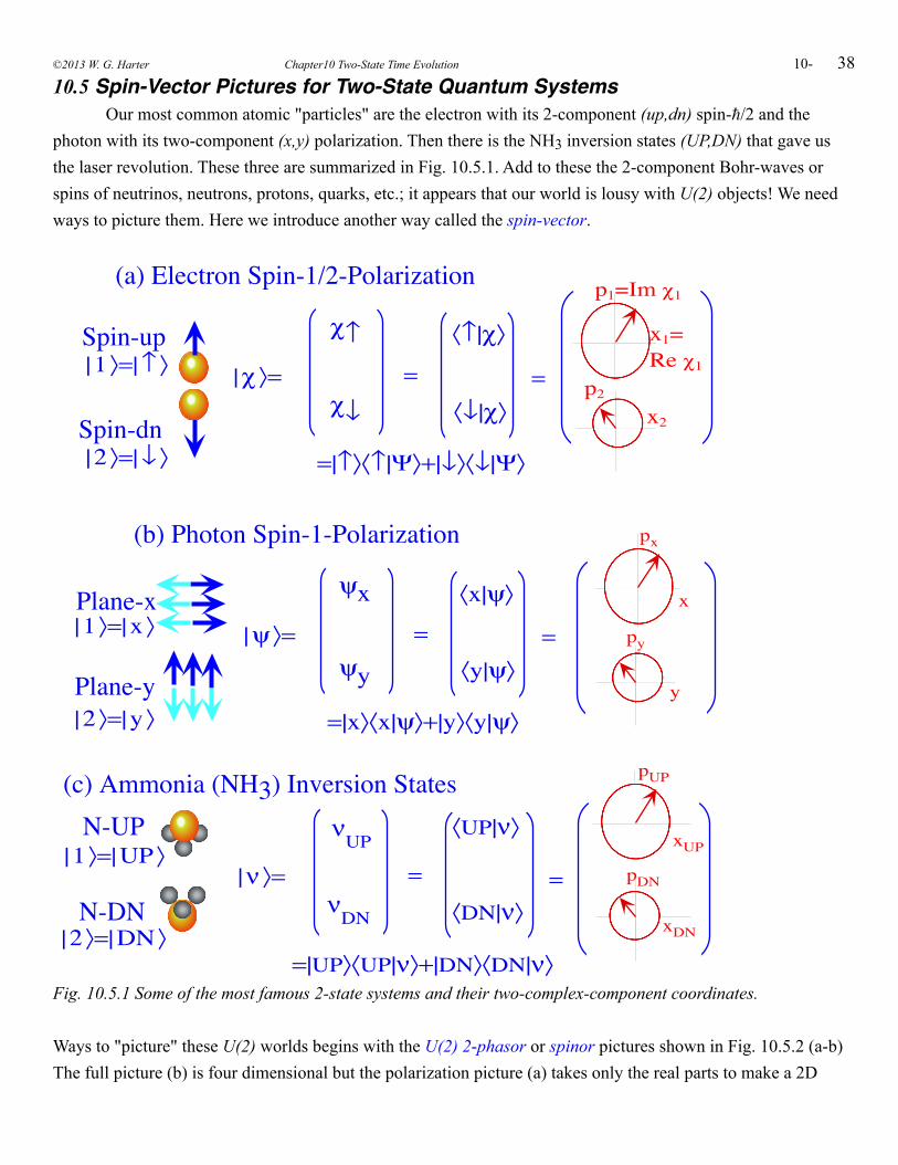
3810.5 Spin-Vector Pictures for Two-State Quantum Systems Our most common atomic "particles" are the electron with its 2-component (up,dn) spin-/2 and the photon with its two-component (x,y) polarization. Then there is the NH3 inversion states (UP,DN) that gave us the laser revolution. These three are summarized in Fig. 10.5.1. Add to these the 2-component Bohr-waves or spins of neutrinos, neutrons, protons, quarks, etc.; it appears that our world is lousy with U(2) objects! We need ways to picture them. Here we introduce another way called the spin-vector.
|χ〉=
χ↑
χ↓=
x1=Re χ1
p1=Im χ1
=
〈↑|χ〉
〈↓|χ〉
=|↑〉〈↑|Ψ〉+|↓〉〈↓|Ψ〉
(a) Electron Spin-1/2-Polarization
Spin-up
Spin-dn
|ψ〉=
ψx
ψy
= =
〈x|ψ〉
〈y|ψ〉
=|x〉〈x|ψ〉+|y〉〈y|ψ〉
(b) Photon Spin-1-Polarization
Plane-x
Plane-y
(c) Ammonia (NH3) Inversion StatesN-UP
N-DN|ν〉=
νUP
νDN
=
xDN
pDN=
〈UP|ν〉
〈DN|ν〉
=|UP〉〈UP|ν〉+|DN〉〈DN|ν〉
xUP
pUP
y
py
x
px
p2x2
| 1 〉=|↑〉
| 2 〉=|↓〉
| 1 〉=|x 〉
| 2 〉=|y 〉
| 1 〉=|UP 〉
| 2 〉=|DN 〉
Fig. 10.5.1 Some of the most famous 2-state systems and their two-complex-component coordinates. Ways to "picture" these U(2) worlds begins with the U(2) 2-phasor or spinor pictures shown in Fig. 10.5.2 (a-b) The full picture (b) is four dimensional but the polarization picture (a) takes only the real parts to make a 2D
©2013 W. G. Harter Chapter10 Two-State Time Evolution 10-
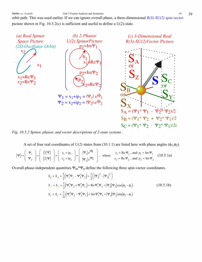
39orbit path. This was used earlier. If we can ignore overall phase, a three-dimensional R(3)-SU(2) spin-vector picture shown in Fig. 10.5.2(c) is sufficient and useful to define a U(2)-state.
x1=ReΨ1
p1=ImΨ1
x2=ReΨ2
p2=ImΨ2
Ψ1 = x1+ip1 = |Ψ1| eiφ1
(b) 2-PhasorU(2) SpinorPicture
φ1
φ2
Ψ2 = x2+ip2 = |Ψ2| eiφ2
(c) 3-Dimensional RealR(3)-SU(2)Vector Picture
SAorSZ SC
or
SYSBor
SXSA = (Ψ1* Ψ1 - Ψ2* Ψ2)/2SB = (Ψ1* Ψ2 + Ψ2* Ψ1)/2SC = (Ψ1* Ψ2 - Ψ2* Ψ1)/2i
Sx1
x2
(a) Real SpinorSpace Picture
x1=ReΨ1x2=ReΨ2
(2D-Oscillator Orbit)
Fig. 10.5.2 Spinor, phasor, and vector descriptions of 2-state systems .
A set of four real coordinates of U(2) states from (10.1.1) are listed here with phase angles (φ1,φ2).
Ψ =Ψ1
Ψ2
⎛
⎝⎜⎜
⎞
⎠⎟⎟=
1 Ψ
2 Ψ
⎛
⎝⎜⎜
⎞
⎠⎟⎟=
x1 + ip1
x2 + ip2
⎛
⎝⎜⎜
⎞
⎠⎟⎟=
Ψ1 eiφ1
Ψ2 eiφ2
⎛
⎝
⎜⎜⎜
⎞
⎠
⎟⎟⎟
, where: x1 = ReΨ1 , and: p1 = ImΨ1
x2 = ReΨ2 , and: p2 = ImΨ2 (10.5.1a)
Overall-phase-independent quantities Ψm*Ψn define the following three spin-vector coordinates.
SZ = SA = 12
Ψ1*Ψ1 −Ψ2
*Ψ2( ) = 12
Ψ12− Ψ2
2⎛⎝
⎞⎠
SX = SB = 12
Ψ1*Ψ2 +Ψ2
*Ψ1( ) = ReΨ1*Ψ2 = Ψ1 Ψ2 cos φ2 −φ1( )
SY = SC = 12i
Ψ1*Ψ2 −Ψ2
*Ψ1( ) = ImΨ1*Ψ2 = Ψ1 Ψ2 sin φ2 −φ1( )
(10.5.1b)
HarterSoft –LearnIt Unit 3 Fourier Analysis and Symmetry 10-
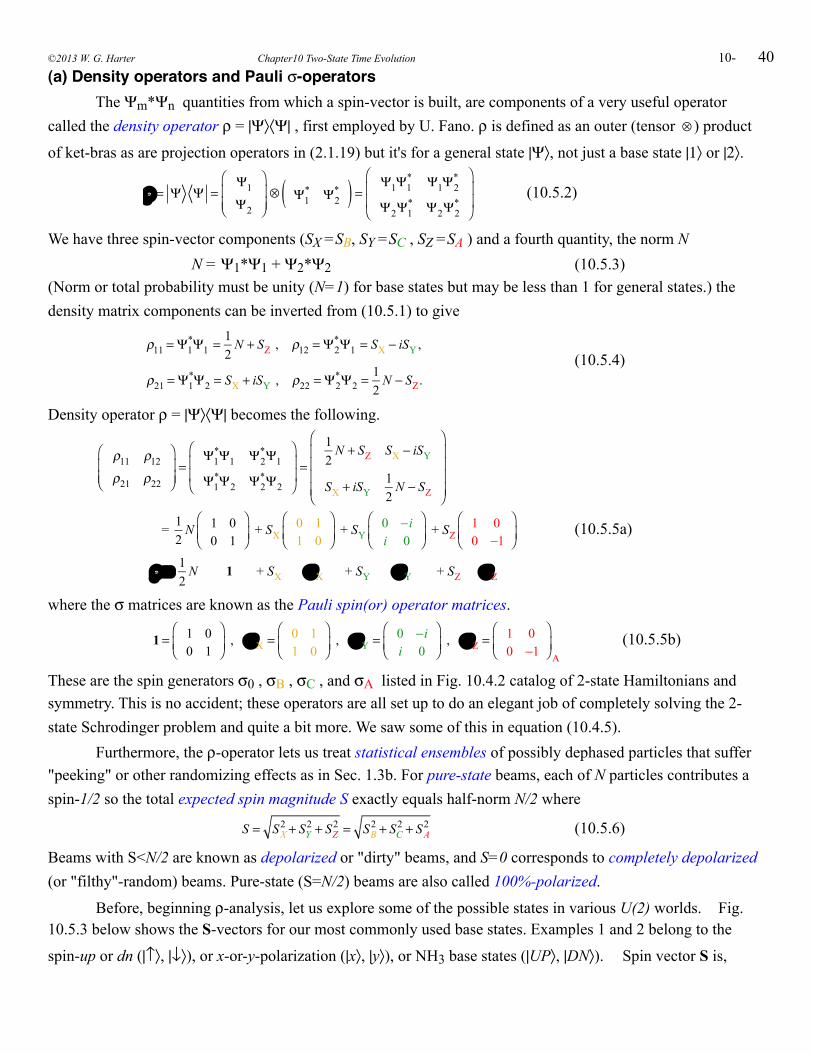
40(a) Density operators and Pauli σ-operators The Ψm*Ψn quantities from which a spin-vector is built, are components of a very useful operator called the density operator ρ = |Ψ〉〈Ψ| , first employed by U. Fano. ρ is defined as an outer (tensor ⊗ ) product
of ket-bras as are projection operators in (2.1.19) but it's for a general state |Ψ〉, not just a base state |1〉 or |2〉.
ρ = Ψ Ψ =Ψ1
Ψ2
⎛
⎝⎜⎜
⎞
⎠⎟⎟⊗ Ψ1
* Ψ2*( ) = Ψ1Ψ1
* Ψ1Ψ2*
Ψ2Ψ1* Ψ2Ψ2
*
⎛
⎝
⎜⎜
⎞
⎠
⎟⎟
(10.5.2)
We have three spin-vector components (SX =SB, SY =SC , SZ =SA ) and a fourth quantity, the norm N N = Ψ1*Ψ1 + Ψ2*Ψ2 (10.5.3)(Norm or total probability must be unity (N=1) for base states but may be less than 1 for general states.) the density matrix components can be inverted from (10.5.1) to give
ρ11 = Ψ1*Ψ1 = 1
2N + SZ , ρ12 = Ψ2
*Ψ1 = SX − iSY,
ρ21 = Ψ1*Ψ2 = SX + iSY , ρ22 = Ψ2
*Ψ2 =12
N − SZ. (10.5.4)
Density operator ρ = |Ψ〉〈Ψ| becomes the following.
ρ11 ρ12
ρ21 ρ22
⎛
⎝⎜⎜
⎞
⎠⎟⎟
=Ψ1
*Ψ1 Ψ2*Ψ1
Ψ1*Ψ2 Ψ2
*Ψ2
⎛
⎝
⎜⎜
⎞
⎠
⎟⎟
=
12
N + SZ SX − iSY
SX + iSY12
N − SZ
⎛
⎝
⎜⎜⎜⎜
⎞
⎠
⎟⎟⎟⎟
= 12
N 1 00 1
⎛
⎝⎜⎞
⎠⎟ + SX
0 11 0
⎛
⎝⎜⎞
⎠⎟ + SY
0 −ii 0
⎛
⎝⎜⎞
⎠⎟ + SZ
1 00 −1
⎛
⎝⎜⎞
⎠⎟
ρ = 12
N 1 + SX σX + SY σY + SZ σZ
(10.5.5a)
where the σ matrices are known as the Pauli spin(or) operator matrices.
1 = 1 0
0 1⎛
⎝⎜⎞
⎠⎟ , σX = 0 1
1 0⎛
⎝⎜⎞
⎠⎟ , σY = 0 −i
i 0⎛
⎝⎜⎞
⎠⎟ , σZ = 1 0
0 −1⎛
⎝⎜⎞
⎠⎟A
(10.5.5b)
These are the spin generators σ0 , σB , σC , and σA listed in Fig. 10.4.2 catalog of 2-state Hamiltonians and symmetry. This is no accident; these operators are all set up to do an elegant job of completely solving the 2-state Schrodinger problem and quite a bit more. We saw some of this in equation (10.4.5). Furthermore, the ρ-operator lets us treat statistical ensembles of possibly dephased particles that suffer "peeking" or other randomizing effects as in Sec. 1.3b. For pure-state beams, each of N particles contributes a spin-1/2 so the total expected spin magnitude S exactly equals half-norm N/2 where
S = SX
2 + SY2 + SZ
2 = SB2 + SC
2 + SA2 (10.5.6)
Beams with S<N/2 are known as depolarized or "dirty" beams, and S=0 corresponds to completely depolarized (or "filthy"-random) beams. Pure-state (S=N/2) beams are also called 100%-polarized.
Before, beginning ρ-analysis, let us explore some of the possible states in various U(2) worlds. Fig. 10.5.3 below shows the S-vectors for our most commonly used base states. Examples 1 and 2 belong to the
spin-up or dn (|↑〉, |↓〉), or x-or-y-polarization (|x〉, |y〉), or NH3 base states (|UP〉, |DN〉). Spin vector S is,
©2013 W. G. Harter Chapter10 Two-State Time Evolution 10-
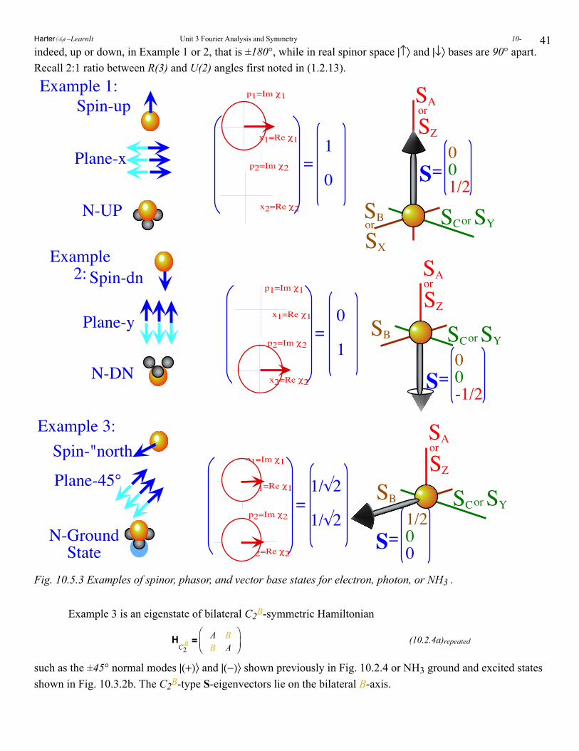
41indeed, up or down, in Example 1 or 2, that is ±180°, while in real spinor space |↑〉 and |↓〉 bases are 90° apart. Recall 2:1 ratio between R(3) and U(2) angles first noted in (1.2.13).
Spin-up
Plane-x
N-UP
x1=Re χ1
p1=Im χ1
x2=Re χ2
p2=Im χ2
SAor
SZ
SCor SYSBorSX
S=1
0001/2
=
Example 1:
x1=Re χ1
p1=Im χ1
x2=Re χ2
p2=Im χ2
SAor
SZSB
S
=0
1 00-1/2
=
Example2: Spin-dn
Plane-y
N-DN
x1=Re χ1
p1=Im χ1
x2=Re χ2
p2=Im χ2
SAor
SZSCor SYSB
S
=1/√2
1/√2 1/200
=
Spin-"north
Plane-45°
N-GroundState
Example 3:
SCor SY
Fig. 10.5.3 Examples of spinor, phasor, and vector base states for electron, photon, or NH3 .
Example 3 is an eigenstate of bilateral C2B-symmetric Hamiltonian
H
C2B =
A BB A
⎛
⎝⎜⎞
⎠⎟ (10.2.4a)repeated
such as the ±45° normal modes |(+)〉 and |(−)〉 shown previously in Fig. 10.2.4 or NH3 ground and excited states shown in Fig. 10.3.2b. The C2B-type S-eigenvectors lie on the bilateral B-axis.
HarterSoft –LearnIt Unit 3 Fourier Analysis and Symmetry 10-
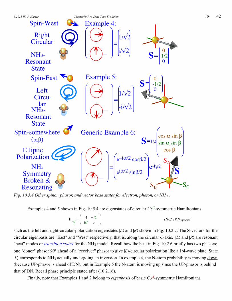
42
=1/√2
i/√2 01/20
=
Spin-West
RightCircular
NH3-ResonantState
Example 4:
=1/√2
-i/√2
0-1/20
=Spin-East Example 5:
S
SLeftCircu-lar
=e−iα/2 cosβ/2
cos α sin βsin α sin βcos β
=1/2Spin-somewhere
(α,β)Generic Example 6:
S
NH3
SymmetryBroken &Resonating
EllipticPolarization
eiα/2 sinβ/2e-iγ/2 S
NH3-ResonantState
SA
SB SCFig. 10.5.4 Other spinor, phasor, and vector base states for electron, photon, or NH3 .
Examples 4 and 5 shown in Fig. 10.5.4 are eigenstates of circular C2C-symmetric Hamiltonians
H
C2C =
A −iCiC A
⎛
⎝⎜⎞
⎠⎟ (10.2.19d)repeated
such as the left and right-circular-polarization eigenstates |L〉 and |R〉 shown in Fig. 10.2.7. The S-vectors for the circular eigenbasis are "East" and "West" respectively, that is, along the circular C-axis. |L〉 and |R〉 are resonant "beat" modes or transition states for the NH3 model. Recall how the beat in Fig. 10.2.6 briefly has two phasors; one "donor" phasor 90° ahead of a "receiver" phasor to give |L〉-circular polarization like a 1/4-wave plate. State |L〉 corresponds to NH3 actually undergoing an inversion. In example 4, the N-atom probability is moving down (because UP-phasor is ahead of DN), but in Example 5 the N-atom is moving up since the UP-phasor is behind that of DN. Recall phase principle stated after (10.2.16). Finally, note that Examples 1 and 2 belong to eigenbasis of basic C2A-symmetric Hamiltonians
©2013 W. G. Harter Chapter10 Two-State Time Evolution 10-
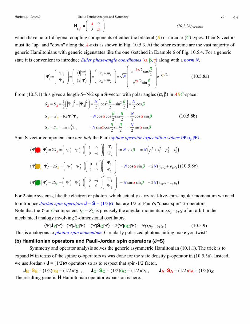
43
H
C2A =
A 00 D
⎛
⎝⎜⎞
⎠⎟ (10.2.2h)repeated
which have no off-diagonal coupling components of either the bilateral (B) or circular (C) types. Their S-vectors must lie "up" and "down" along the A-axis as shown in Fig. 10.5.3. At the other extreme are the vast majority of generic Hamiltonians with generic eigenstates like the one sketched in Example 6 of Fig. 10.5.4. For a generic state it is convenient to introduce Euler phase-angle coordinates (α, β, γ) along with a norm N.
Ψ =Ψ1
Ψ2
⎛
⎝⎜⎜
⎞
⎠⎟⎟=
1 Ψ
2 Ψ
⎛
⎝⎜⎜
⎞
⎠⎟⎟=
x1 + ip1
x2 + ip2
⎛
⎝⎜⎜
⎞
⎠⎟⎟= N
e−iα /2 cosβ2
eiα /2 sinβ2
⎛
⎝
⎜⎜⎜⎜
⎞
⎠
⎟⎟⎟⎟
e−iγ /2 (10.5.8a)
From (10.5.1) this gives a length-S=N/2 spin S-vector with polar angles (α, β) in ABC-space!
SZ = SA = 12
Ψ12− Ψ2
2⎛⎝
⎞⎠ =
N2
cos2 β2− sin2 β
2⎛⎝⎜
⎞⎠⎟= N
2cosβ
SX = SB = ReΨ1*Ψ2 = N cosα cos
β2
sinβ2
= N2
cosα sinβ
SY = SC = ImΨ1*Ψ2 = N sinα cos
β2
sinβ2
= N2
sinα sinβ
(10.5.8b)
Spin S-vector components are one-half the Pauli spinor operator expectation values 〈Ψ|σµ|Ψ〉 .
Ψ σZ Ψ = 2SA = Ψ1* Ψ2
*( ) 1 00 −1
⎛
⎝⎜⎞
⎠⎟Ψ1
Ψ2
⎛
⎝⎜⎜
⎞
⎠⎟⎟
= N cosβ = N p12 + x1
2 − p22 − x2
2( )
Ψ σX
Ψ = 2SB = Ψ1* Ψ2
*( ) 0 11 0
⎛
⎝⎜⎞
⎠⎟Ψ1
Ψ2
⎛
⎝⎜⎜
⎞
⎠⎟⎟
= N cosα sinβ = 2N x1x2 + p1p2( )
Ψ σY Ψ = 2SC = Ψ1* Ψ2
*( ) 0 −ii 0
⎛
⎝⎜⎞
⎠⎟Ψ1
Ψ2
⎛
⎝⎜⎜
⎞
⎠⎟⎟
= N sinα sinβ = 2N x1p2 − x2 p1( )
(10.5.8c)
For 2-state systems, like the electron or photon, which actually carry real-live-spin-angular momentum we need to introduce Jordan spin operators J = S = (1/2)σ that are 1/2 of Pauli's "quasi-spin" σ-operators.Note that the Y-or C-component JC = SC is precisely the angular momentum xpy - ypx of an orbit in the mechanical analogy involving 2-dimensional oscillators. 〈Ψ|JY|Ψ〉 =〈Ψ|JC|Ψ〉 = 〈Ψ|SC|Ψ〉 = 2〈Ψ|σC|Ψ〉 = N(xpy - ypx ) (10.5.9)This is analogous to photon-spin momentum. Circularly polarized photons hitting make you twist!
(b) Hamiltonian operators and Pauli-Jordan spin operators (J=S) Symmetry and operator analysis solves the generic asymmetric Hamiltonian (10.1.1). The trick is to expand H in terms of the spinor σ-operators as was done for the state density ρ-operator in (10.5.5a). Instead, we use Jordan's J = (1/2)σ operators so as to respect that spin-1/2 factor. JB=SB = (1/2)σB = (1/2)σX , JC=SC = (1/2)σC = (1/2)σY , JA=SA = (1/2)σA = (1/2)σZ The resulting generic H Hamiltonian operator expansion is here.
HarterSoft –LearnIt Unit 3 Fourier Analysis and Symmetry 10-
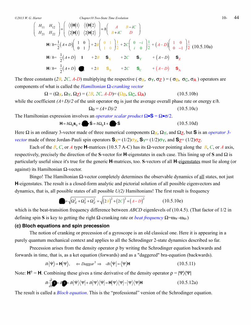
44
H11 H12
H21 H22
⎛
⎝⎜⎜
⎞
⎠⎟⎟=
1 H 1 1 H 2
2 H 1 2 H 2
⎛
⎝⎜⎜
⎞
⎠⎟⎟= A B − iC
B + iC D
⎛
⎝⎜⎞
⎠⎟
H / = 12
A+ D( ) 1 00 1
⎛
⎝⎜⎞
⎠⎟ + 2B 0 1
1 0⎛
⎝⎜⎞
⎠⎟12
+ 2C 0 −ii 0
⎛
⎝⎜⎞
⎠⎟12
+ A− D( ) 1 00 −1
⎛
⎝⎜⎞
⎠⎟12
H / = 12
A+ D( ) 1 + 2B SX + 2C SY + A− D( ) SZ
H / = 12
A+ D( ) σ0 + 2B SB + 2C SC + A− D( ) SA
(10.5.10a)
The three constants (2B, 2C, A-D) multiplying the respective ( σX, σY, σZ ) = ( σB, σC, σA ) operators are components of what is called the Hamiltonian Ω-cranking vector Ω = (ΩX, ΩY, ΩZ) = (2B, 2C, A-D)= (ΩB, ΩC, ΩA) (10.5.10b)while the coefficient (A+D)/2 of the unit operator σ0 is just the average overall phase rate or energy ε/. Ω0 = (A+D)/2 (10.5.10c)The Hamiltonian expression involves an operator scalar product Ω•S = Ω•σ/2. H = Ω0s0 + Ω•
S = Ω01+ Ω•
S (10.5.10d)
Here Ω is an ordinary 3-vector made of three numerical components ΩX, ΩY, and ΩZ, but S is an operator 3-vector made of three Jordan-Pauli spin operators SX= (1/2)σX, SY= (1/2)σY, and SZ= (1/2)σZ. Each of the B, C, or A type H-matrices (10.5.7 A-C) has its Ω-vector pointing along the B, C, or A axis, respectively, precisely the direction of the S-vector for H-eigenstates in each case. This lining up of S and Ω is particularly useful since it's true for the generic H-matrices, too. S-vectors of all H-eigenstates must lie along (or against) its Hamiltonian Ω-vector.
Bingo! The Hamiltonian Ω-vector completely determines the observable dynamics of all states, not just H-eigenstates. The result is a closed-form analytic and pictorial solution of all possible eigenvectors and dynamics, that is, all possible states of all possible U(2) Hamiltonians! The first result is frequency
Ω = ΩX
2 +ΩY2 +ΩZ
2 = 2B( )2 + 2C( )2 + A− D( )2 (10.5.10e)
which is the beat-transition frequency difference between ABCD eigenlevels of (10.4.5). (That factor of 1/2 in defining spin S is key to getting the right Ω-cranking rate or beat frequency Ω=ωhi -ωlo.)
(c) Bloch equations and spin precession The notion of cranking or precession of a gyroscope is an old classical one. Here it is appearing in a purely quantum mechanical context and applies to all the Schrodinger 2-state dynamics described so far.
Precession arises from the density operator ρ by writing the Schrodinger equation backwards and forwards in time, that is, as a ket equation (forwards) and as a "daggered" bra-equation (backwards).
i Ψ =H Ψ , ⇐ Daggar† ⇒ -i Ψ = Ψ H (10.5.11)
Note: H† = H. Combining these gives a time derivative of the density operator ρ = |Ψ〉〈Ψ|
i ∂∂ t
ρ = i ρ = i Ψ Ψ + i Ψ Ψ =H Ψ Ψ − Ψ Ψ H (10.5.12a)
The result is called a Bloch equation. This is the “professional” version of the Schrodinger equation.
©2013 W. G. Harter Chapter10 Two-State Time Evolution 10-
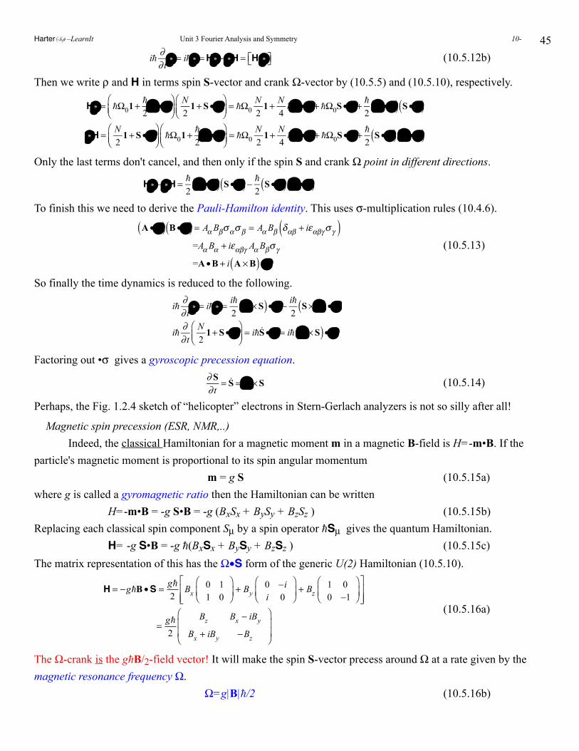
45
i ∂∂ t
ρ = i ρ =Hρ − ρH = H,ρ⎡⎣ ⎤⎦ (10.5.12b)
Then we write ρ and H in terms spin S-vector and crank Ω-vector by (10.5.5) and (10.5.10), respectively.
Hρ = Ω01+ 2Ω •σ
⎛⎝⎜
⎞⎠⎟
N2
1+ S•σ⎛⎝⎜
⎞⎠⎟= Ω0
N2
1+ N4Ω•σ + Ω0S•σ +
2Ω •σ( ) S•σ( )
ρH = N2
1+ S•σ⎛⎝⎜
⎞⎠⎟Ω01+
2Ω •σ
⎛⎝⎜
⎞⎠⎟= Ω0
N2
1+ N4Ω•σ + Ω0S•σ +
2S•σ( ) Ω •σ( )
Only the last terms don't cancel, and then only if the spin S and crank Ω point in different directions.
Hρ − ρH =
2Ω •σ( ) S•σ( )− 2 S•σ( ) Ω •σ( )
To finish this we need to derive the Pauli-Hamilton identity. This uses σ-multiplication rules (10.4.6).
A •σ( ) B•σ( ) = Aα Bβσασβ = Aα Bβ δαβ + iεαβγσγ( ) =Aα Bα + iεαβγ Aα Bβσγ
=A •B + i A ×B( ) ⋅ σ (10.5.13)
So finally the time dynamics is reduced to the following.
i ∂∂ t
ρ = i ρ = i2
Ω× S( )•σ − i2
S×Ω( )•σ
i ∂∂ t
N2
1+ S•σ⎛⎝⎜
⎞⎠⎟= i S•σ = i Ω× S( )•σ
Factoring out •σ gives a gyroscopic precession equation.
∂ S∂ t
= S = Ω× S (10.5.14)
Perhaps, the Fig. 1.2.4 sketch of “helicopter” electrons in Stern-Gerlach analyzers is not so silly after all!
Magnetic spin precession (ESR, NMR,..) Indeed, the classical Hamiltonian for a magnetic moment m in a magnetic B-field is H=-m•B. If the particle's magnetic moment is proportional to its spin angular momentum m = g S (10.5.15a)where g is called a gyromagnetic ratio then the Hamiltonian can be written H=-m•B = -g S•B = -g (BxSx + BySy + BzSz ) (10.5.15b)Replacing each classical spin component Sµ by a spin operator Sµ gives the quantum Hamiltonian. H= -g S•B = -g (BxSx + BySy + BzSz ) (10.5.15c)The matrix representation of this has the Ω•S form of the generic U(2) Hamiltonian (10.5.10).
H = −gB •S = g2
Bx0 11 0
⎛
⎝⎜⎞
⎠⎟+ By
0 −ii 0
⎛
⎝⎜⎞
⎠⎟+ Bz
1 00 −1
⎛
⎝⎜⎞
⎠⎟⎡
⎣⎢⎢
⎤
⎦⎥⎥
= g2
Bz Bx − iBy
Bx + iBy −Bz
⎛
⎝⎜⎜
⎞
⎠⎟⎟
(10.5.16a)
The Ω-crank is the gB/2-field vector! It will make the spin S-vector precess around Ω at a rate given by the magnetic resonance frequency Ω. Ω=g|B|/2 (10.5.16b)
HarterSoft –LearnIt Unit 3 Fourier Analysis and Symmetry 10-
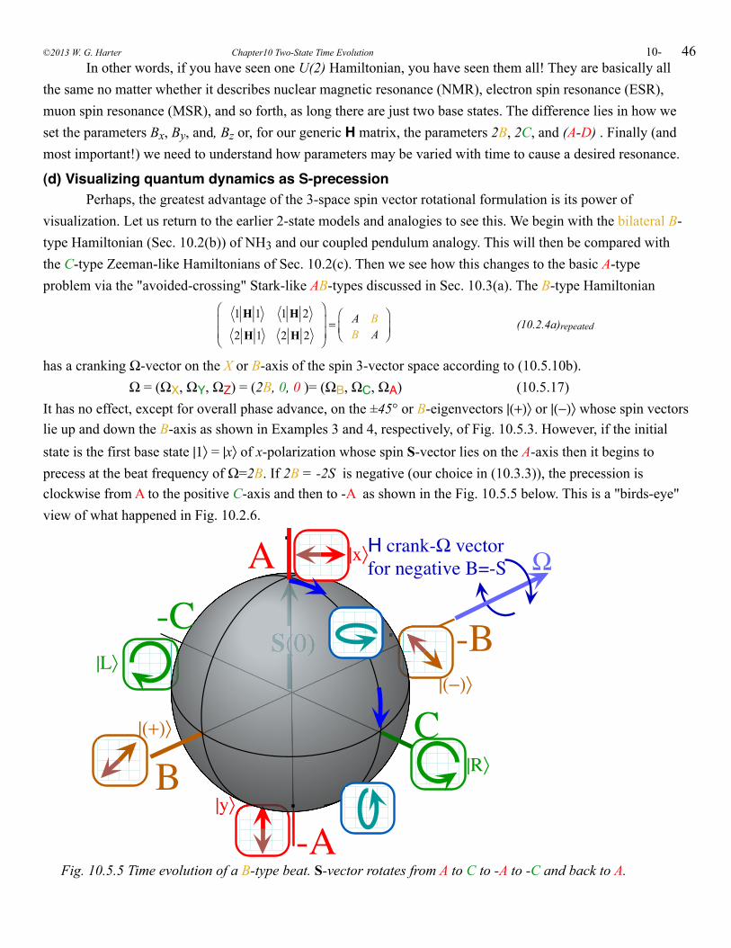
46 In other words, if you have seen one U(2) Hamiltonian, you have seen them all! They are basically all the same no matter whether it describes nuclear magnetic resonance (NMR), electron spin resonance (ESR), muon spin resonance (MSR), and so forth, as long there are just two base states. The difference lies in how we set the parameters Bx, By, and, Bz or, for our generic H matrix, the parameters 2B, 2C, and (A-D) . Finally (and most important!) we need to understand how parameters may be varied with time to cause a desired resonance.
(d) Visualizing quantum dynamics as S-precession Perhaps, the greatest advantage of the 3-space spin vector rotational formulation is its power of visualization. Let us return to the earlier 2-state models and analogies to see this. We begin with the bilateral B-type Hamiltonian (Sec. 10.2(b)) of NH3 and our coupled pendulum analogy. This will then be compared with the C-type Zeeman-like Hamiltonians of Sec. 10.2(c). Then we see how this changes to the basic A-type problem via the "avoided-crossing" Stark-like AB-types discussed in Sec. 10.3(a). The B-type Hamiltonian
1 H 1 1 H 2
2 H 1 2 H 2
⎛
⎝⎜⎜
⎞
⎠⎟⎟= A B
B A⎛
⎝⎜⎞
⎠⎟ (10.2.4a)repeated
has a cranking Ω-vector on the X or B-axis of the spin 3-vector space according to (10.5.10b). Ω = (ΩX, ΩY, ΩZ) = (2B, 0, 0 )= (ΩB, ΩC, ΩA) (10.5.17)It has no effect, except for overall phase advance, on the ±45° or B-eigenvectors |(+)〉 or |(−)〉 whose spin vectors lie up and down the B-axis as shown in Examples 3 and 4, respectively, of Fig. 10.5.3. However, if the initial state is the first base state |1〉 = |x〉 of x-polarization whose spin S-vector lies on the A-axis then it begins to precess at the beat frequency of Ω=2B. If 2B = -2S is negative (our choice in (10.3.3)), the precession is clockwise from A to the positive C-axis and then to -A as shown in the Fig. 10.5.5 below. This is a "birds-eye" view of what happened in Fig. 10.2.6.
A
-A
C
-C
B
-B
H crank-Ω vectorfor negative B=-S
|(+)〉
|(−)〉
|R〉
|L〉
|x〉
|y〉
Ω
Fig. 10.5.5 Time evolution of a B-type beat. S-vector rotates from A to C to -A to -C and back to A.
©2013 W. G. Harter Chapter10 Two-State Time Evolution 10-
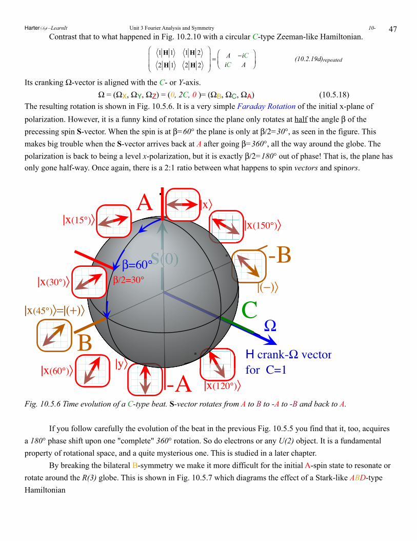
47 Contrast that to what happened in Fig. 10.2.10 with a circular C-type Zeeman-like Hamiltonian.
1 H 1 1 H 2
2 H 1 2 H 2
⎛
⎝⎜⎜
⎞
⎠⎟⎟= A −iC
iC A⎛
⎝⎜⎞
⎠⎟ (10.2.19d)repeated
Its cranking Ω-vector is aligned with the C- or Y-axis. Ω = (ΩX, ΩY, ΩZ) = (0, 2C, 0 )= (ΩB, ΩC, ΩA) (10.5.18)The resulting rotation is shown in Fig. 10.5.6. It is a very simple Faraday Rotation of the initial x-plane of polarization. However, it is a funny kind of rotation since the plane only rotates at half the angle β of the precessing spin S-vector. When the spin is at β=60° the plane is only at β/2=30°, as seen in the figure. This makes big trouble when the S-vector arrives back at A after going β=360°, all the way around the globe. The polarization is back to being a level x-polarization, but it is exactly β/2=180° out of phase! That is, the plane has only gone half-way. Once again, there is a 2:1 ratio between what happens to spin vectors and spinors.
|x(120°)〉
A
-A
CB
-B
H crank-Ω vectorfor C=1
|x(45°)〉=|(+)〉
|(−)〉
|x〉
|y〉
Ω
|x(30°)〉
|x(15°)〉
|x(60°)〉
|x(150°)〉
β/2=30°β=60°
Fig. 10.5.6 Time evolution of a C-type beat. S-vector rotates from A to B to -A to -B and back to A.
If you follow carefully the evolution of the beat in the previous Fig. 10.5.5 you find that it, too, acquires a 180° phase shift upon one "complete" 360° rotation. So do electrons or any U(2) object. It is a fundamental property of rotational space, and a quite mysterious one. This is studied in a later chapter. By breaking the bilateral B-symmetry we make it more difficult for the initial A-spin state to resonate or rotate around the R(3) globe. This is shown in Fig. 10.5.7 which diagrams the effect of a Stark-like ABD-type Hamiltonian
HarterSoft –LearnIt Unit 3 Fourier Analysis and Symmetry 10-
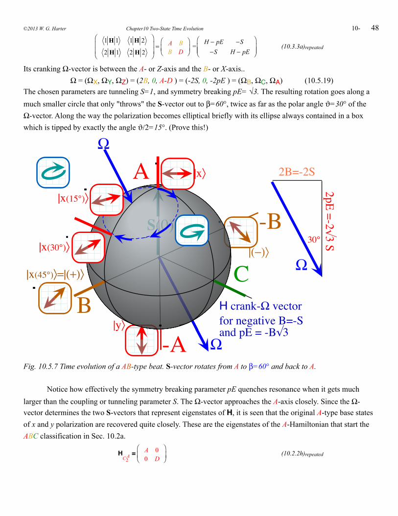
48
1 H 1 1 H 2
2 H 1 2 H 2
⎛
⎝⎜⎜
⎞
⎠⎟⎟= A B
B D
⎛
⎝⎜⎞
⎠⎟ =
H − pE −S−S H − pE
⎛
⎝⎜⎜
⎞
⎠⎟⎟
(10.3.3a)repeated
Its cranking Ω-vector is between the A- or Z-axis and the B- or X-axis.. Ω = (ΩX, ΩY, ΩZ) = (2B, 0, A-D ) = (-2S, 0, -2pE ) = (ΩB, ΩC, ΩA) (10.5.19)The chosen parameters are tunneling S=1, and symmetry breaking pE= √3. The resulting rotation goes along a much smaller circle that only "throws" the S-vector out to β=60°, twice as far as the polar angle ϑ=30° of the Ω-vector. Along the way the polarization becomes elliptical briefly with its ellipse always contained in a box which is tipped by exactly the angle ϑ/2=15°. (Prove this!)
A
-A
CB
-B
H crank-Ω vectorfor negative B=-Sand pE = -B√3
|x(45°)〉=|(+)〉
|(−)〉
|x〉
|y〉
Ω
|x(30°)〉
|x(15°)〉
Ω
Ω
2B=-2S
2pE=-2√3
S30°
Fig. 10.5.7 Time evolution of a AB-type beat. S-vector rotates from A to β=60° and back to A.
Notice how effectively the symmetry breaking parameter pE quenches resonance when it gets much larger than the coupling or tunneling parameter S. The Ω-vector approaches the A-axis closely. Since the Ω-vector determines the two S-vectors that represent eigenstates of H, it is seen that the original A-type base states of x and y polarization are recovered quite closely. These are the eigenstates of the A-Hamiltonian that start the ABC classification in Sec. 10.2a.
H
C2A =
A 00 D
⎛
⎝⎜⎞
⎠⎟ (10.2.2h)repeated
©2013 W. G. Harter Chapter10 Two-State Time Evolution 10-
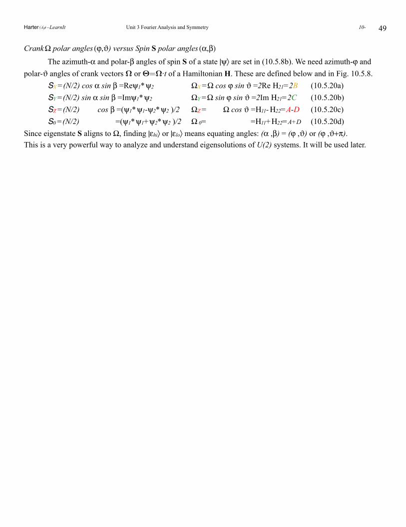
49
Crank Ω polar angles (ϕ,ϑ) versus Spin S polar angles (α,β)
The azimuth-α and polar-β angles of spin S of a state |ψ〉 are set in (10.5.8b). We need azimuth-ϕ and polar-ϑ angles of crank vectors Ω or Θ=Ω·t of a Hamiltonian H. These are defined below and in Fig. 10.5.8. SX =(N/2) cos α sin β =Reψ1* ψ2 ΩX =Ω cos ϕ sin ϑ =2Re Η21=2B (10.5.20a) SY =(N/2) sin α sin β =Imψ1* ψ2 ΩY =Ω sin ϕ sin ϑ =2Im Η21=2C (10.5.20b) SZ =(N/2) cos β =(ψ1* ψ1-ψ2* ψ2 )/2 ΩZ = Ω cos ϑ =Η11- Η22=A-D (10.5.20c) S0 =(N/2) =(ψ1* ψ1+ψ2* ψ2 )/2 Ω 0= : =Η11+Η22=A+D (10.5.20d)Since eigenstate S aligns to Ω, finding |εhi〉 or |εlo〉 means equating angles: (α ,β) = (ϕ ,ϑ) or (ϕ ,ϑ+π).This is a very powerful way to analyze and understand eigensolutions of U(2) systems. It will be used later.
HarterSoft –LearnIt Unit 3 Fourier Analysis and Symmetry 10-
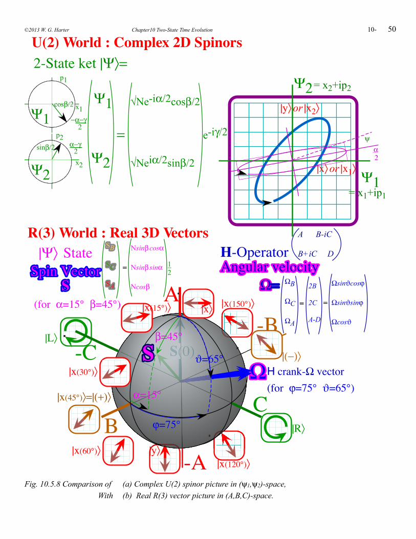
50
-B-C
|R〉
|L〉
|x(120°)〉
A
-A
CB
H crank-Ω vector(for ϕ=75° ϑ=65°)
|x(45°)〉=|(+)〉
|(−)〉
|x〉
|y〉
ΩΩ|x(30°)〉
|x(15°)〉
|x(60°)〉
|x(150°)〉
β=45°
ϑ=65°
ϕ=75°
α=15°
R(3) World : Real 3D Vectors
SS
H-OperatorAAnngguullaarr vveelloocciittyy
ΩΩ==
|Ψ〉 StateSSppiinn VVeeccttoorr
SS
Ψ1
Ψ2
2-State ket |Ψ〉=
Ψ1
Ψ2
=
√Ne-iα/2cosβ/2
e-iγ/2
√Neiα/2sinβ/2
U(2) World : Complex 2D Spinors
Ψ2
α−γsinβ/2 2x2
p2
Ψ1 −α−γ
cosβ/2
2
x1
p1 = x2+ip2
= x1+ip1
|x〉or |x1〉
|y〉or |x2〉
A B-iC
B+iC D
ΩB
ΩC
ΩA
2B
2C
A-D
Ωsinϑcosϕ
Ωsinϑsinϕ
Ωcosϑ
==
SSBB
SSCC
SSAA
Nsinβcosα
Nsinβ sinα
Ncosβ
=
(for α=15° β=45°)
12
α2
ψ
Fig. 10.5.8 Comparison of (a) Complex U(2) spinor picture in (ψ1,ψ2)-space,With (b) Real R(3) vector picture in (A,B,C)-space.
©2013 W. G. Harter Chapter10 Two-State Time Evolution 10-
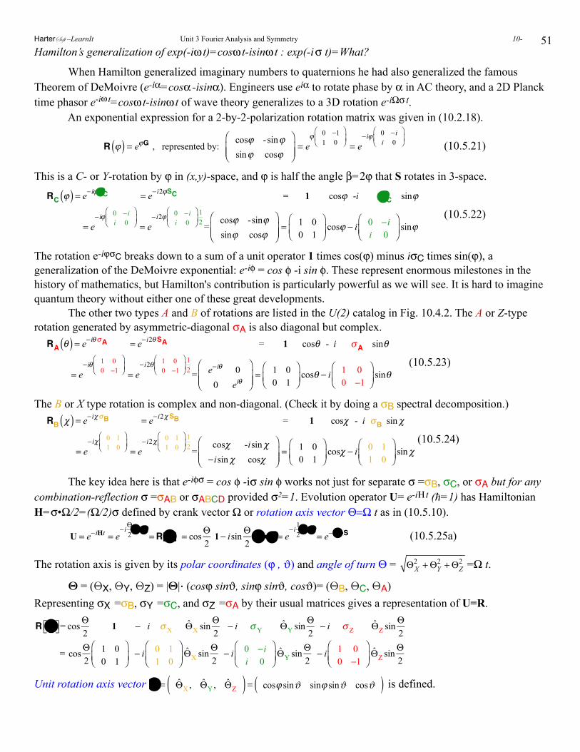
51Hamilton’s generalization of exp(-iω t)=cosω t-isinω t : exp(-i σ t)=What?
When Hamilton generalized imaginary numbers to quaternions he had also generalized the famous Theorem of DeMoivre (e-iα=cosα -isinα). Engineers use eiα to rotate phase by α in AC theory, and a 2D Planck time phasor e-iω t=cosω t-isinω t of wave theory generalizes to a 3D rotation e-iΩσ t. An exponential expression for a 2-by-2-polarization rotation matrix was given in (10.2.18).
R ϕ( ) = eϕG , represented by:
cosϕ - sinϕsinϕ cosϕ
⎛
⎝⎜⎜
⎞
⎠⎟⎟= e
ϕ 0 −11 0
⎛
⎝⎜⎞
⎠⎟ = e−iϕ 0 −i
i 0
⎛
⎝⎜⎞
⎠⎟ (10.5.21)
This is a C- or Y-rotation by ϕ in (x,y)-space, and ϕ is half the angle β=2ϕ that S rotates in 3-space.
RC ϕ( ) = e−iϕσC = e−i2ϕSC = 1 cosϕ -i σC sinϕ
= e−iϕ 0 −i
i 0
⎛
⎝⎜⎞
⎠⎟ = e−i2ϕ 0 −i
i 0
⎛
⎝⎜⎞
⎠⎟12 =
cosϕ -sinϕsinϕ cosϕ
⎛
⎝⎜⎜
⎞
⎠⎟⎟= 1 0
0 1
⎛
⎝⎜⎞
⎠⎟cosϕ − i 0 −i
i 0
⎛
⎝⎜⎞
⎠⎟sinϕ
(10.5.22)
The rotation e-iϕσC breaks down to a sum of a unit operator 1 times cos(ϕ) minus iσC times sin(ϕ), a generalization of the DeMoivre exponential: e-iφ = cos φ -i sin φ. These represent enormous milestones in the history of mathematics, but Hamilton's contribution is particularly powerful as we will see. It is hard to imagine quantum theory without either one of these great developments. The other two types A and B of rotations are listed in the U(2) catalog in Fig. 10.4.2. The A or Z-type rotation generated by asymmetric-diagonal σA is also diagonal but complex.
RA θ( ) = e−iθσA = e−i2θSA = 1 cosθ - i σA sinθ
= e−iθ 1 0
0 −1
⎛
⎝⎜⎞
⎠⎟ = e−i2θ 1 0
0 −1
⎛
⎝⎜⎞
⎠⎟12 = e−iθ 0
0 eiθ
⎛
⎝⎜⎜
⎞
⎠⎟⎟= 1 0
0 1
⎛
⎝⎜⎞
⎠⎟cosθ − i 1 0
0 −1
⎛
⎝⎜⎞
⎠⎟sinθ
(10.5.23)
The B or X type rotation is complex and non-diagonal. (Check it by doing a σB spectral decomposition.)
RB χ( ) = e−iχσB = e−i2χSB = 1 cosχ - i σB sinχ
= e−iχ 0 1
1 0
⎛
⎝⎜⎞
⎠⎟ = e−i2χ 0 1
1 0
⎛
⎝⎜⎞
⎠⎟12 =
cosχ -isinχ−isinχ cosχ
⎛
⎝⎜⎜
⎞
⎠⎟⎟= 1 0
0 1
⎛
⎝⎜⎞
⎠⎟cosχ − i 0 1
1 0
⎛
⎝⎜⎞
⎠⎟sinχ
(10.5.24)
The key idea here is that e-iφσ = cos φ -iσ sin φ works not just for separate σ =σB, σC, or σA but for any combination-reflection σ =σAB or σABCD provided σ2=1. Evolution operator U= e-iΗ t (=1) has Hamiltonian H=σ•Ω/2=(Ω/2)σ defined by crank vector Ω or rotation axis vector Θ=Ω t as in (10.5.10).
U = e−iHt = e
−iΘ2Θ•σ
=R[Θ] = cosΘ2
1− isinΘ2
Θ •σ = e−i1
2Θ•σ
= e−iΘ•S (10.5.25a)
The rotation axis is given by its polar coordinates (ϕ , ϑ) and angle of turn Θ = ΘX
2 +ΘY2 +ΘZ
2 =Ω t.
Θ = (ΘX, ΘY, ΘZ) = |Θ|· (cosϕ sinϑ, sinϕ sinϑ, cosϑ)= (ΘB, ΘC, ΘA) Representing σX =σB, σY =σC, and σZ =σA by their usual matrices gives a representation of U=R.
R Θ⎡⎣ ⎤⎦= cosΘ2
1 − i σX ΘX sinΘ2
− i σY ΘY sinΘ2
− i σ Z ΘZ sinΘ2
= cosΘ2
1 00 1
⎛
⎝⎜⎞
⎠⎟ − i 0 1
1 0
⎛
⎝⎜⎞
⎠⎟ΘX sin
Θ2
− i 0 −ii 0
⎛
⎝⎜⎞
⎠⎟ΘY sin
Θ2
− i 1 00 −1
⎛
⎝⎜⎞
⎠⎟ΘZ sin
Θ2
Unit rotation axis vector Θ = ΘX, ΘY, ΘZ( ) = cosϕ sinϑ sinϕ sinϑ cosϑ( ) is defined.
HarterSoft –LearnIt Unit 3 Fourier Analysis and Symmetry 10-
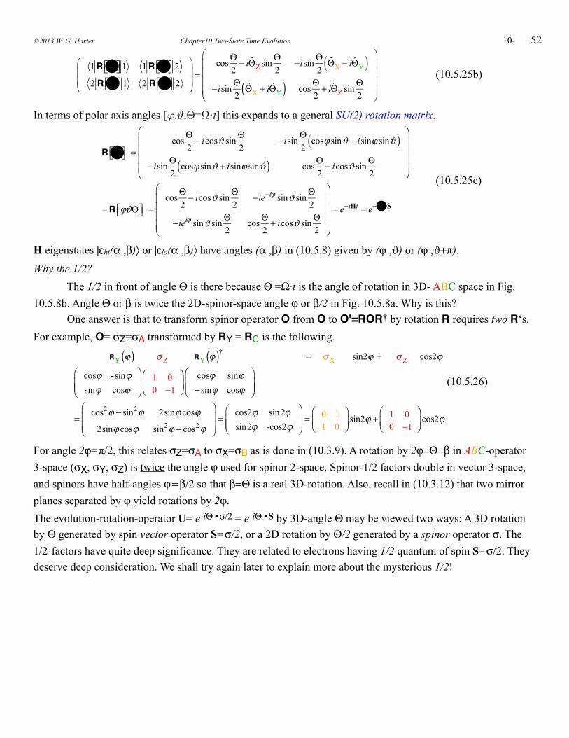
52
1R Θ⎡⎣ ⎤⎦ 1 1R Θ⎡⎣ ⎤⎦ 2
2 R Θ⎡⎣ ⎤⎦ 1 2 R Θ⎡⎣ ⎤⎦ 2
⎛
⎝⎜⎜
⎞
⎠⎟⎟=
cosΘ2− iΘZ sin
Θ2
−isinΘ2
ΘX − iΘY( )−isinΘ
2ΘX + iΘY( ) cos
Θ2+ iΘZ sin
Θ2
⎛
⎝
⎜⎜⎜⎜
⎞
⎠
⎟⎟⎟⎟
(10.5.25b)
In terms of polar axis angles [ϕ,ϑ,Θ=Ω·t] this expands to a general SU(2) rotation matrix.
R Θ⎡⎣ ⎤⎦ =cos
Θ2− icosϑ sin
Θ2
−isinΘ2
cosϕ sinϑ − isinϕ sinϑ( )
−isinΘ2
cosϕ sinϑ + isinϕ sinϑ( ) cosΘ2+ icosϑ sin
Θ2
⎛
⎝
⎜⎜⎜⎜
⎞
⎠
⎟⎟⎟⎟
=R ϕϑΘ⎡⎣ ⎤⎦ =cos
Θ2− icosϑ sin
Θ2
−ie−iϕ sinϑ sinΘ2
−ieiϕ sinϑ sinΘ2
cosΘ2+ icosϑ sin
Θ2
⎛
⎝
⎜⎜⎜⎜
⎞
⎠
⎟⎟⎟⎟
= e−iHt = e−iΘ•S
(10.5.25c)
H eigenstates |εhi(α ,β)〉 or |εlo(α ,β)〉 have angles (α ,β) in (10.5.8) given by (ϕ ,ϑ) or (ϕ ,ϑ+π).
Why the 1/2? The 1/2 in front of angle Θ is there because Θ =Ω·t is the angle of rotation in 3D- ABC space in Fig. 10.5.8b. Angle Θ or β is twice the 2D-spinor-space angle ϕ or β/2 in Fig. 10.5.8a. Why is this? One answer is that to transform spinor operator O from O to O'=ROR† by rotation R requires two R‘s. For example, O= σZ=σA transformed by RY = RC is the following.
RY ϕ( ) σ Z RY ϕ( )† = σX sin2ϕ + σ Z cos2ϕ
cosϕ -sinϕsinϕ cosϕ
⎛
⎝⎜⎜
⎞
⎠⎟⎟
1 00 −1
⎛
⎝⎜⎞
⎠⎟cosϕ sinϕ−sinϕ cosϕ
⎛
⎝⎜⎜
⎞
⎠⎟⎟
=cos2ϕ − sin2ϕ 2sinϕ cosϕ
2sinϕ cosϕ sin2ϕ − cos2ϕ
⎛
⎝⎜⎜
⎞
⎠⎟⎟=
cos2ϕ sin2ϕsin2ϕ -cos2ϕ
⎛
⎝⎜⎜
⎞
⎠⎟⎟= 0 1
1 0
⎛
⎝⎜⎞
⎠⎟sin2ϕ + 1 0
0 −1
⎛
⎝⎜⎞
⎠⎟cos2ϕ
(10.5.26)
For angle 2ϕ=π/2, this relates σZ=σA to σX=σB as is done in (10.3.9). A rotation by 2ϕ=Θ=β in ABC-operator 3-space (σX, σY, σZ) is twice the angle ϕ used for spinor 2-space. Spinor-1/2 factors double in vector 3-space, and spinors have half-angles ϕ = β/2 so that β=Θ is a real 3D-rotation. Also, recall in (10.3.12) that two mirror planes separated by ϕ yield rotations by 2ϕ. The evolution-rotation-operator U= e-iΘ • σ/2 = e-iΘ • S by 3D-angle Θ may be viewed two ways: A 3D rotation by Θ generated by spin vector operator S=σ/2, or a 2D rotation by Θ/2 generated by a spinor operator σ. The 1/2-factors have quite deep significance. They are related to electrons having 1/2 quantum of spin S=σ/2. They deserve deep consideration. We shall try again later to explain more about the mysterious 1/2!
©2013 W. G. Harter Chapter10 Two-State Time Evolution 10-
53Problems for Chapter 10.ABCDanonical? 10.1.1. The canonical definition of momentum does not always give pj=m dxj/dt. (See “Deep Classical..” Chapter 5.3)
(a) What is the general definition of pj in terms of a Lagrangian L? First, what is L in terms of Hamiltonian H? (b) Find L and pj for the classical ABCD Hamiltonian (10.1.3c).(c) Is the Schrodinger-to-Classical-Oscillator analogy correct if there is explicit time dependence A(t), B(t),..etc.?
All fall down10.1.2. The fall-line at any point in a 2D potential V(x,y) is determined by ∇V (or -∇V, which?)
(a) Relate acceleration-force vector (10.1.5) for the general potential V=(1/2)x•A•x (10.1.6b) to the gradient ∇V.(b) Find eigenvectors and eigenvalues of acceleration matrix A . Show how eigenvectors relate to V-ellipse axes for:.
case A: (A=4, D=1, B=0, C=0) , case B: (A=D=4, B=-1, C=0) , case AB: (A=4, D=1, B=1, C=0) .Relate each to a classical normal mode frequency.
(c) Find eigenvectors and eigenvalues of Hamiltonian matrix H for:.case A: (A=4, D=1, B=0, C=0) , case B: (A=D=4, B=-1, C=0) , case AB: (A=4, D=1, B=1, C=0) .Relate each to a quantum energy or eigenfrequency.
Groupie quaternions10.1.3 Do the quaternions {1, i, j, k} by themselves make a group? How about Pauli { σ1, σA , σB , σC }?
(a) How about the set { 1, i, j, k , -1, -i, -j, -k} ? Construct a 4x4 multiplication table for {1, i, j, k}.(b) How about the set { σ1,σA ,σB ,σC ,-σ1,-σA ,-σB ,-σC } ? Construct a 4x4 multiplication table.[c] Show that σm · σn = δmn1 + iemnp σp .
__________________________________________________________________Use the Phase Luke!10.2.1 Suppose a particle is oscillating at frequency ω according to x(t) = A sin (ω t) while experiencing an applied force at the same frequency but ahead in phase angle φ according to F(t) = F sin (ω t-φ) .
(a) Does positive φ represent a force ahead or behind ?(b) Sketch a F versus x (Work-cycle) diagram for φ = 0 , π/4, π/2, π, and 3π/2 .(c) Calculate the work F does on x each cycle as a function of φ and indicate how it relates to area of F-x plots (b).(d) At the moment shown in Fig. 10.2.6, what is the phase angle φ between x1 and x2. Who’s ahead? How does the phase
angle vary with time? How does the energy flow (in the classical model) between the two vary with time?
__________________________________________________________________B versus C10.3.1The H-matrix for the symmetry B, and C was given in the form of the tunneling amplitudes (B=-S) plus magnetic Zeeman (dipole) energy shifts (C ) . As the relative magnitudes of these vary the eigenstates, eigenvalues, and symmetry changes, too.
(a) Write the H(H, B, C=0) matrix in a basis that is most appropriate for its (What? B, or C?)-symmetry and use the lowest order perturbation theory to describe the effect of small C-value. Compare your result to that of the exact avoided crossing eigenvalues for (B=1, C=0.2). Describe the set or group of matrix operators that commute with H(H, B, C=0) and with H(H, B=1, C=0.2) , that is, give both finite "rotation" matrices and their generators. Sketch eigenstate phasor and polarization diagrams† for each case.Sketch ABC Ω and S vector diagrams† for each case.(b) Write the H(H, B=0, C) matrix in a basis that is most appropriate for its (What? B, or C?)-symmetry and use the lowest order perturbation theory to describe the effect of small B-value. Compare your result to that of the exact avoided crossing eigenvalues for (B=0.2, C=1). Describe the set or group of matrix operators that commute with H(H, B=0, C) and with H(H, B=0.2, C=1) , that is, give both finite "rotation" matrices and their generators.Sketch eigenstate phasor and polarization diagrams† for each case.Sketch ABC Ω and S vector diagrams† for each case. †See Sec. 10.5.
Commute or else!10.3.2 Use spectral decompositions to derive the form of the general U(2) matrix that commutes...
(a) ...with σ A = 1 0
0 −1
⎛
⎝⎜⎞
⎠⎟ (b) ...with
σ B = 0 1
1 0
⎛
⎝⎜⎞
⎠⎟ ,(c) ...with
σC = 0 −i
i 0
⎛
⎝⎜⎞
⎠⎟ , (d) ...with
M = 4 1
3 2
⎛
⎝⎜⎞
⎠⎟.
(e to h) Derive the form of the most general SU(2) matrices that commute with each of the above.
HarterSoft –LearnIt Unit 3 Fourier Analysis and Symmetry 10-
54
Eigenvalues easy as ABCD10.4.1 The expansion (10.4.5b-c) gives a closed form expression for eigenvalues of a general HABCD.
(a) Verify all parts of (10.4.5).(b) Show the eigenvalues so obtained agree with a direct diagonalization of HABCD.(c) Show that this is a special case of HAB eigenvalues in (10.3.11).
Ellipses on ellipses10.4.2 The elliptical eigenstate orbits of Fig. 10.4.1 are seen to correspond to the elliptical equipotential level curves.
(a) Do they really? How so?(b) Work the eigensolutions for Fig. 10.4.1 and plot their ellipses.(c) Are the ellipse major axes of orthogonal eigenvectors themselves orthogonal? Why or why not?
_____________________________________________________Eigenvectors easy as ABCD10.5.1 The prescription (10.5.20) for finding general U(2) eigenvectors is powerful and important.
(a) Write it out in detail for the AB-Hamiltonian in Fig. 10.5.7. Give eigenstates easily. (Recall (10.5.8a)(b) Show how a polarization ellipse would evolve and fill a rectangle if x-polarization were fed to this H.(c) Do similarly with the Hamiltonian and initial spin shown in Fig. 10.5.8.
Very cross prodots10.5.2 Using the σ-operator definitions and the Levi-Civita tensor definition
derive the following. (First prove Levi-Civita rule: εabcεdec = δadδbe − δaeδbd )
(a) σ aσb = δab + i εabcσ c
c∑ (b) σ aσbσ a = 2δabσ a − σb (c)
σ •A( ) σ •B( ) = A •B( ) + i A ×B( )•σ
Spinor round10.5.3 Use spectral decomposition to derive three rotation operators(A-C) and base transforms (d-g).
(a)
R θxy( ) = e−iθxy
2σ z = 1cos
θxy
2− iσ z sin
θxy
2= e
−iθxy / 20
0 eiθxy / 2
⎛
⎝⎜⎜
⎞
⎠⎟⎟
(b) R θ yz( ) = e
−iθ yz
2σ x = 1cos
θ yz
2− iσ x sin
θ yz
2=
______ ____________ ______
⎛
⎝⎜⎜
⎞
⎠⎟⎟
(c) R θzx( ) = e
−iθzx
2σ y = 1cos
θzx2
− iσ y sinθzx2
=______ ____________ ______
⎛
⎝⎜⎜
⎞
⎠⎟⎟
(d) R θab( ) ⋅1 ⋅R† θab( ) = 1
(e) R θab( ) ⋅σ a ⋅R
† θab( ) = σ a cosθab +σb sinθab
(f) R θab( ) ⋅σb ⋅R
† θab( ) = −σ a sinθab +σb cosθab
(g) R θab( ) ⋅σ c ⋅R
† θab( ) = σ c (Let:εabc =1)
The Lorentz district10.5.4 Use spectral decomposition to derive three Lorentz operators (A-C) and base transforms (d-f).
(a)
L θtz( ) = eθtz2σ z = 1cosh
θtz2
+σ z sinhθtz2
= eθtz / 2 0
0 e−θtz / 2
⎛
⎝⎜⎜
⎞
⎠⎟⎟
(b) L θtx( ) = e
θtx2
σ x = 1coshθtx2
+σ x sinhθtx2
=______ ____________ ______
⎛
⎝⎜⎜
⎞
⎠⎟⎟
©2013 W. G. Harter Chapter10 Two-State Time Evolution 10-
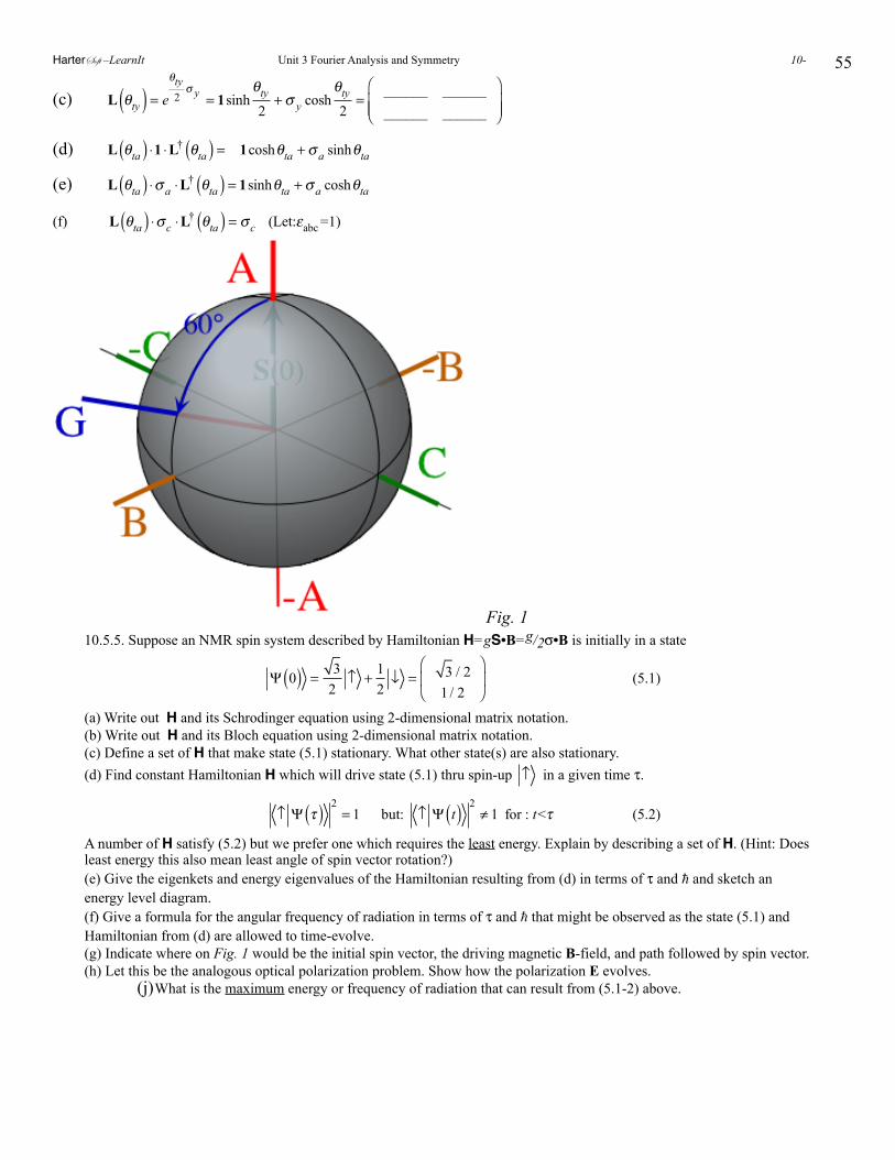
55
(c) L θty( ) = e
θty2
σ y = 1sinhθty
2+σ y cosh
θty
2=
______ ____________ ______
⎛
⎝⎜⎜
⎞
⎠⎟⎟
(d) L θta( ) ⋅1 ⋅L† θta( ) = 1coshθta +σ a sinhθta
(e) L θta( ) ⋅σ a ⋅L
† θta( ) = 1sinhθta +σ a coshθta
(f) L θta( ) ⋅σ c ⋅L
† θta( ) = σ c (Let:εabc =1)
Fig. 110.5.5. Suppose an NMR spin system described by Hamiltonian H=gS•B=g/2σ•B is initially in a state
Ψ 0( ) = 3
2↑ + 1
2↓ = 3 / 2
1 / 2
⎛
⎝⎜
⎞
⎠⎟ (5.1)
(a) Write out H and its Schrodinger equation using 2-dimensional matrix notation.(b) Write out H and its Bloch equation using 2-dimensional matrix notation.(c) Define a set of H that make state (5.1) stationary. What other state(s) are also stationary.(d) Find constant Hamiltonian H which will drive state (5.1) thru spin-up ↑ in a given time τ.
↑ Ψ τ( ) 2
= 1 but: ↑ Ψ t( ) 2≠ 1 for : t<τ (5.2)
A number of H satisfy (5.2) but we prefer one which requires the least energy. Explain by describing a set of H. (Hint: Does least energy this also mean least angle of spin vector rotation?)(e) Give the eigenkets and energy eigenvalues of the Hamiltonian resulting from (d) in terms of τ and and sketch an energy level diagram.(f) Give a formula for the angular frequency of radiation in terms of τ and that might be observed as the state (5.1) and Hamiltonian from (d) are allowed to time-evolve. (g) Indicate where on Fig. 1 would be the initial spin vector, the driving magnetic B-field, and path followed by spin vector.(h) Let this be the analogous optical polarization problem. Show how the polarization E evolves.
(j)What is the maximum energy or frequency of radiation that can result from (5.1-2) above.
HarterSoft –LearnIt Unit 3 Fourier Analysis and Symmetry 10-

56©2013 W. G. Harter Chapter10 Two-State Time Evolution 10-
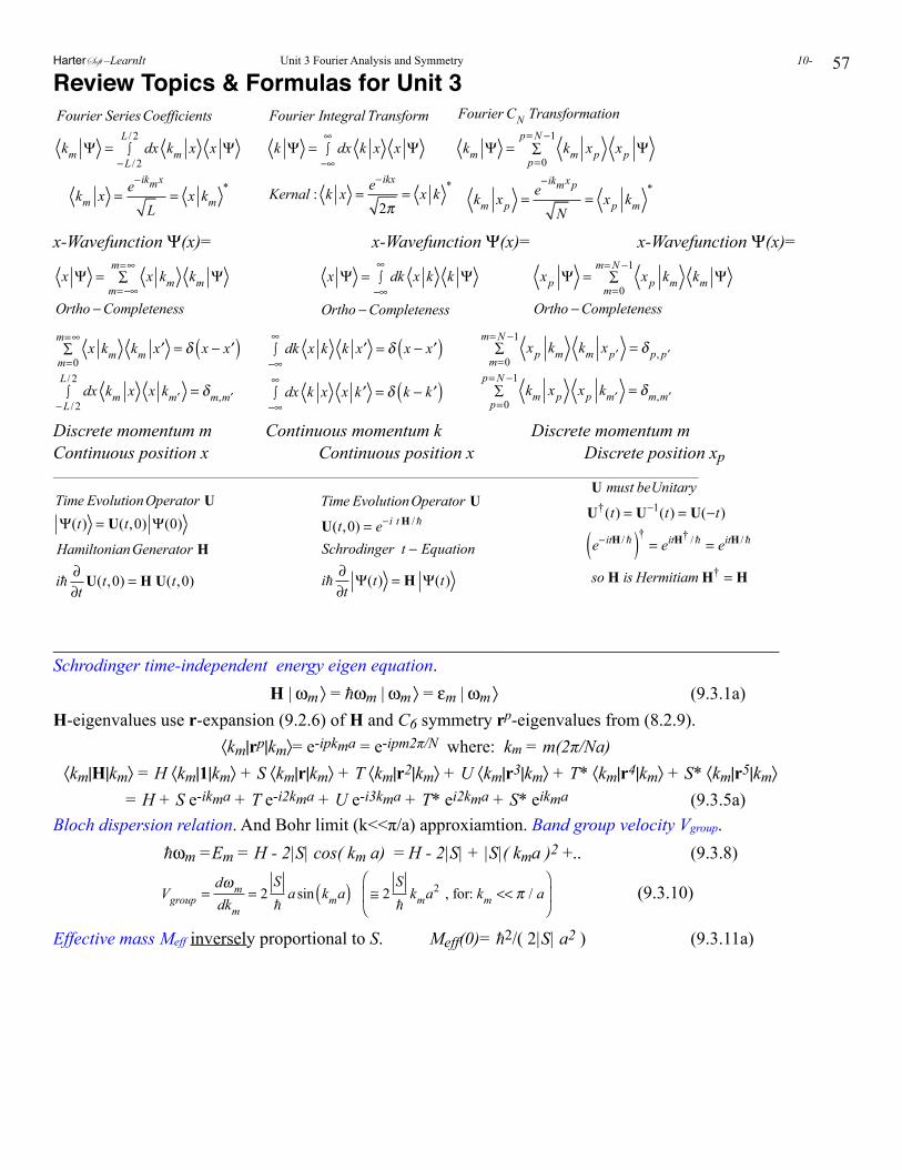
57Review Topics & Formulas for Unit 3
Fourier SeriesCoefficients
km Ψ = dx−L / 2
L / 2∫ km x x Ψ
km x = e−ikmx
L= x km
*
Fourier Integral Transform
k Ψ = dx−∞
∞∫ k x x Ψ
Kernal : k x = e−ikx
2π= x k
*
Fourier CN Transformation
km Ψ = km xp xp Ψp=0
p=N −1∑
km xp = e−ikmxp
N= xp km
*
x-Wavefunction Ψ(x)= x-Wavefunction Ψ(x)= x-Wavefunction Ψ(x)=
x Ψ = x km km Ψm=−∞
m=∞∑
Ortho −Completeness
x Ψ = dk−∞
∞∫ x k k Ψ
Ortho −Completeness
xp Ψ = xp km km Ψm=0
m=N −1∑
Ortho −Completeness
x km km ′xm=0
m=∞∑ = δ x − ′x( )
dx−L / 2
L / 2∫ km x x k ′m = δm, ′m
dk−∞
∞∫ x k k ′x = δ x − ′x( )
dx−∞
∞∫ k x x ′k = δ k − ′k( )
xp km km x ′pm=0
m=N −1∑ = δ p, ′p
km xp xp k ′mp=0
p=N −1∑ = δm, ′m
Discrete momentum m Continuous momentum k Discrete momentum mContinuous position x Continuous position x Discrete position xp_____________________________________________________________________________________________________________________________
Time EvolutionOperator UΨ(t) = U(t,0) Ψ(0)
HamiltonianGenerator H
i ∂∂t
U(t,0) = H U(t,0)
Time EvolutionOperator U
U(t,0) = e−i t H /
Schrodinger t − Equation
i ∂∂t
Ψ(t) = H Ψ(t)
U must beUnitary
U†(t) = U−1(t) = U(−t)
e−itH /( )† = eitH† / = eitH /
so H is Hermitiam H† = H
__________________________________________________________________________________Schrodinger time-independent energy eigen equation. H | ωm 〉 = ωm | ωm 〉 = εm | ωm 〉 (9.3.1a)H-eigenvalues use r-expansion (9.2.6) of H and C6 symmetry rp-eigenvalues from (8.2.9). 〈km|rp|km〉= e-ipkma = e-ipm2π/N where: km = m(2π/Na) 〈km|H|km〉 = H 〈km|1|km〉 + S 〈km|r|km〉 + T 〈km|r2|km〉 + U 〈km|r3|km〉 + T* 〈km|r4|km〉 + S* 〈km|r5|km〉: = H + S e-ikma + T e-i2kma + U e-i3kma + T* ei2kma + S* eikma (9.3.5a) Bloch dispersion relation. And Bohr limit (k<<π/a) approxiamtion. Band group velocity Vgroup. ωm =Em = H - 2|S| cos( km a) = H - 2|S| + |S|( kma )2 +.. (9.3.8)
Vgroup =dωmdkm
= 2S
a sin kma( ) ≅ 2
S
kma2 , for: km << π / a
⎛
⎝⎜
⎞
⎠⎟ (9.3.10)
Effective mass Meff inversely proportional to S. Meff(0)= 2/( 2|S| a2 ) (9.3.11a)
HarterSoft –LearnIt Unit 3 Fourier Analysis and Symmetry 10-
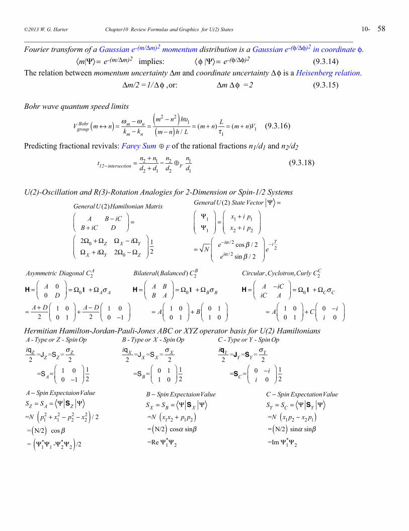
58__________________________________________________________________________________Fourier transform of a Gaussian e-(m/Δm)2 momentum distribution is a Gaussian e-(φ/Δφ)2 in coordinate φ. 〈m|Ψ〉 = e-(m/Δm)2 implies: 〈 φ |Ψ〉 = e-(φ/Δφ)2 (9.3.14)The relation between momentum uncertainty Δm and coordinate uncertainty Δ φ is a Heisenberg relation. Δm/2 =1/ Δ φ , or: Δm Δ φ =2 (9.3.15)
Bohr wave quantum speed limits
Vgroup
Bohr m ↔ n( ) = ωm −ωnkm − kn
=m2 − n2( )hυ1
m − n( )h / L= (m + n) L
τ1= (m + n)V1 (9.3.16)
Predicting fractional revivals: Farey Sum ⊕ F of the rational fractions n1/d1 and n2/d2
t12− intersection =
n2 + n1d2 + d1
=n2d2
⊕Fn1d1
(9.3.18)
U(2)-Oscillation and R(3)-Rotation Analogies for 2-Dimension or Spin-1/2 Systems
GeneralU (2)Hamiltonian Matrix
A B − iCB + iC D
⎛
⎝⎜⎞
⎠⎟=
2Ω0 +ΩZ ΩX − iΩY
ΩX + iΩY 2Ω0 − ΩZ
⎛
⎝⎜⎜
⎞
⎠⎟⎟
12
GeneralU (2) State Vector Ψ =
Ψ1
Ψ1
⎛
⎝⎜⎜
⎞
⎠⎟⎟=
x1 + i p1
x2 + i p2
⎛
⎝⎜⎜
⎞
⎠⎟⎟
= Ne−iα / 2 cosβ / 2
eiα / 2 sinβ / 2
⎛
⎝⎜⎜
⎞
⎠⎟⎟
e−i
γ2
Asymmetric Diagonal C2A
H = A 00 D
⎛
⎝⎜⎞
⎠⎟= Ω01 +ΩAσ A
= A+ D2
1 00 1
⎛
⎝⎜⎞
⎠⎟+ A− D
21 00 −1
⎛
⎝⎜⎞
⎠⎟
Bilateral(Balanced ) C2B
H = A BB A
⎛
⎝⎜⎞
⎠⎟= Ω01 +ΩBσ B
= A 1 00 1
⎛
⎝⎜⎞
⎠⎟+ B 0 1
1 0
⎛
⎝⎜⎞
⎠⎟
Circular,Cyclotron,Curly C2C
H = A −iCiC A
⎛
⎝⎜⎞
⎠⎟= Ω01 +ΩCσC
= A 1 00 1
⎛
⎝⎜⎞
⎠⎟+ C 0 −i
i 0
⎛
⎝⎜⎞
⎠⎟
Hermitian Hamilton-Jordan-Pauli-Jones ABC or XYZ operator basis for U(2) Hamiltonians
A - Type or Z - Spin OpiqZ2
=JZ =SZ =σZ2
=SA= 1 00 −1
⎛
⎝⎜⎞
⎠⎟12
B - Type or X - Spin OpiqX
2=JX =SX =
σ X2
=SB = 0 11 0
⎛
⎝⎜⎞
⎠⎟12
C - Type or Y - Spin OpiqY2
=JY =SY =σY2
=SC = 0 −ii 0
⎛
⎝⎜⎞
⎠⎟12
A− Spin ExpectaionValue
SZ = SA = Ψ SZ Ψ
=N p12 + x1
2 − p22 − x2
2( ) / 2
= N/2( ) cosβ
= Ψ1*Ψ1 -Ψ2
*Ψ2( ) /2
B − Spin ExpectaionValue
SX = SB = Ψ SX Ψ
=N x1x2 + p1p2( ) = N/2( ) cosα sinβ
=Re Ψ1*Ψ2
C − Spin ExpectationValue
SY = SC = Ψ SY Ψ
=N x1p2 − x2 p1( ) = N/2( ) sinα sinβ
=Im Ψ1*Ψ2
©2013 W. G. Harter Chapter10 Review Formulas and Graphics for U(2) States 10-
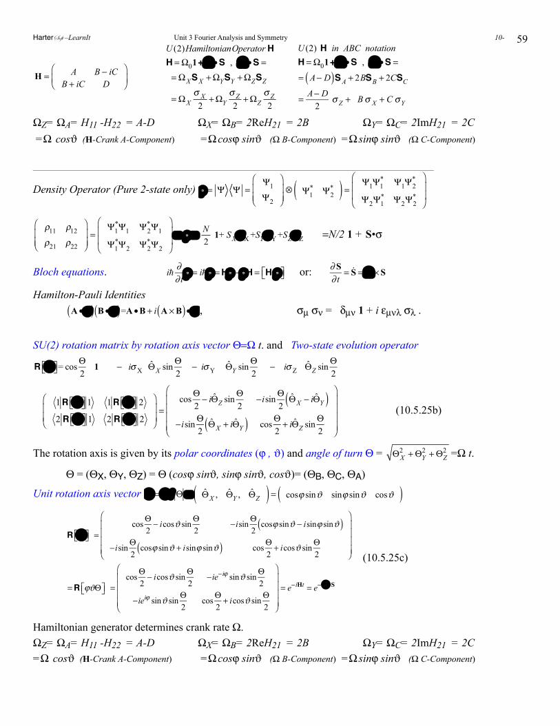
59
H = A B − iC
B + iC D⎛
⎝⎜⎞
⎠⎟
U (2)HamiltonianOperatorHH =Ω01+Ω •S , Ω•S =
=ΩXSX +ΩYSY +ΩZSZ
=ΩXσ X
2+ΩY
σ Z2
+ΩZσ Z2
U (2) H in ABC notationH =Ω01+Ω •S , Ω•S =
= A− D( )SA + 2BSB + 2CSC
= A− D2
σ Z + Bσ X + C σY
ΩZ= ΩA= H11 -H22 = A-D ΩX= ΩB= 2ReH21 = 2B ΩY= ΩC= 2ImH21 = 2C =Ω cosϑ (H-Crank A-Component) =Ω cosϕ sinϑ (Ω B-Component) =Ω sinϕ sinϑ (Ω C-Component)
_____________________________________________________________________________________________________________________________
Density Operator (Pure 2-state only)
ρ = Ψ Ψ =Ψ1
Ψ2
⎛
⎝⎜⎜
⎞
⎠⎟⎟⊗ Ψ1
* Ψ2*( ) = Ψ1Ψ1
* Ψ1Ψ2*
Ψ2Ψ1* Ψ2Ψ2
*
⎛
⎝
⎜⎜
⎞
⎠
⎟⎟
ρ11 ρ12
ρ21 ρ22
⎛
⎝⎜⎜
⎞
⎠⎟⎟
=Ψ1
*Ψ1 Ψ2*Ψ1
Ψ1*Ψ2 Ψ2
*Ψ2
⎛
⎝
⎜⎜
⎞
⎠
⎟⎟
= ρ = N2
1+ SXσX +SYσY +SZσZ =N/2 1 + S•σ
Bloch equations. i ∂∂ t
ρ = i ρ =Hρ − ρH = H,ρ⎡⎣ ⎤⎦ or: ∂ S∂ t
= S = Ω× S
Hamilton-Pauli Identities
A •σ( ) B•σ( )=A •B + i A ×B( )•σ , σµ σν = δµν 1 + i εµνλ σλ .
SU(2) rotation matrix by rotation axis vector Θ=Ω t. and Two-state evolution operator
R Θ⎡⎣ ⎤⎦= cos
Θ2
1 − iσX ΘX sinΘ2
− iσY ΘY sinΘ2
− iσ Z ΘZ sinΘ2
1R Θ⎡⎣ ⎤⎦ 1 1R Θ⎡⎣ ⎤⎦ 2
2 R Θ⎡⎣ ⎤⎦ 1 2 R Θ⎡⎣ ⎤⎦ 2
⎛
⎝⎜⎜
⎞
⎠⎟⎟=
cosΘ2− iΘZ sin
Θ2
−isinΘ2
ΘX − iΘY( )−isinΘ
2ΘX + iΘY( ) cos
Θ2+ iΘZ sin
Θ2
⎛
⎝
⎜⎜⎜⎜
⎞
⎠
⎟⎟⎟⎟
(10.5.25b)
The rotation axis is given by its polar coordinates (ϕ , ϑ) and angle of turn Θ = ΘX
2 +ΘY2 +ΘZ
2 =Ω t.
Θ = (ΘX, ΘY, ΘZ) = Θ (cosϕ sinϑ, sinϕ sinϑ, cosϑ)= (ΘB, ΘC, ΘA)
Unit rotation axis vector Θ =Θ / Θ = ΘX , ΘY , ΘZ( ) = cosϕ sinϑ sinϕ sinϑ cosϑ( )
R Θ⎡⎣ ⎤⎦ =cos
Θ2− icosϑ sin
Θ2
−isinΘ2
cosϕ sinϑ − isinϕ sinϑ( )
−isinΘ2
cosϕ sinϑ + isinϕ sinϑ( ) cosΘ2+ icosϑ sin
Θ2
⎛
⎝
⎜⎜⎜⎜
⎞
⎠
⎟⎟⎟⎟
=R ϕϑΘ⎡⎣ ⎤⎦ =cos
Θ2− icosϑ sin
Θ2
−ie−iϕ sinϑ sinΘ2
−ieiϕ sinϑ sinΘ2
cosΘ2+ icosϑ sin
Θ2
⎛
⎝
⎜⎜⎜⎜
⎞
⎠
⎟⎟⎟⎟
= e−iHt = e−iΘ•S
(10.5.25c)
Hamiltonian generator determines crank rate Ω.ΩZ= ΩA= H11 -H22 = A-D ΩX= ΩB= 2ReH21 = 2B ΩY= ΩC= 2ImH21 = 2C=Ω cosϑ (H-Crank A-Component) =Ω cosϕ sinϑ (Ω B-Component) =Ω sinϕ sinϑ (Ω C-Component)
HarterSoft –LearnIt Unit 3 Fourier Analysis and Symmetry 10-
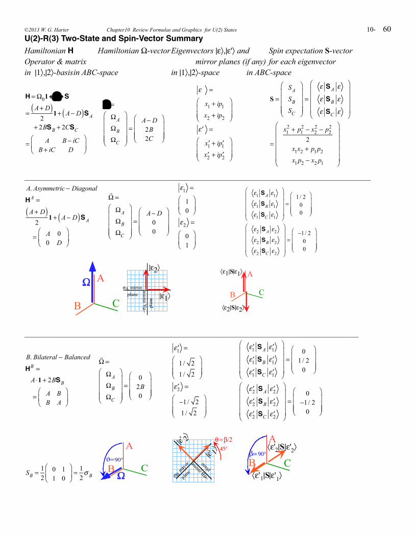
60U(2)-R(3) Two-State and Spin-Vector SummaryHamiltonian H Hamiltonian Ω-vector Eigenvectors |ε〉,|ε'〉 and Spin expectation S-vectorOperator & matrix mirror planes (if any) for each eigenvectorin |1〉,|2〉-basis in ABC-space in |1〉,|2〉-space in ABC-space
H =Ω01+Ω •S
=A+ D( )
21+ A− D( )SA
+ 2BSB + 2CSC
= A B − iCB + iC D
⎛
⎝⎜⎞
⎠⎟
Ω =
ΩA
ΩB
ΩC
⎛
⎝
⎜⎜⎜⎜
⎞
⎠
⎟⎟⎟⎟
=A− D2B2C
⎛
⎝
⎜⎜⎜
⎞
⎠
⎟⎟⎟
ε =
x1 + ip1
x2 + ip2
⎛
⎝⎜⎜
⎞
⎠⎟⎟
′ε =
′x1 + i ′p1
′x2 + i ′p2
⎛
⎝⎜⎜
⎞
⎠⎟⎟
S =
SA
SB
SC
⎛
⎝
⎜⎜⎜⎜
⎞
⎠
⎟⎟⎟⎟
=
ε SA ε
ε SB ε
ε SC ε
⎛
⎝
⎜⎜⎜⎜
⎞
⎠
⎟⎟⎟⎟
=
x12 + p1
2 − x22 − p2
2
2x1x2 + p1p2
x1p2 − x2 p1
⎛
⎝
⎜⎜⎜⎜⎜
⎞
⎠
⎟⎟⎟⎟⎟
_____________________________________________________________________________________
A. Asymmetric − Diagonal
HA =
A+ D( )2
1 + A− D( )SA
= A 00 D
⎛
⎝⎜⎞
⎠⎟
Ω =
ΩA
ΩB
ΩC
⎛
⎝
⎜⎜⎜⎜
⎞
⎠
⎟⎟⎟⎟
=A− D
00
⎛
⎝
⎜⎜⎜
⎞
⎠
⎟⎟⎟
ε1 =
10
⎛
⎝⎜⎞
⎠⎟
ε2 =
01
⎛
⎝⎜⎞
⎠⎟
ε1 SA ε1
ε1 SB ε1
ε1 SC ε1
⎛
⎝
⎜⎜⎜⎜
⎞
⎠
⎟⎟⎟⎟
=1 / 2
00
⎛
⎝
⎜⎜⎜
⎞
⎠
⎟⎟⎟
ε2 SA ε2
ε2 SB ε2
ε2 SC ε2
⎛
⎝
⎜⎜⎜⎜
⎞
⎠
⎟⎟⎟⎟
=−1 / 2
00
⎛
⎝
⎜⎜⎜
⎞
⎠
⎟⎟⎟
B
A
C
Ω
|ε1〉
|ε2〉
σA mirror plane
−σA
mir
ror
p
lane
B
A
C
〈ε1|S|ε1〉
〈ε2|S|ε2〉
__________________________________________________________________________________
B. Bilateral − Balanced
HB =
A ⋅1 + 2BSB
= A BB A
⎛
⎝⎜⎞
⎠⎟
Ω =
ΩA
ΩB
ΩC
⎛
⎝
⎜⎜⎜⎜
⎞
⎠
⎟⎟⎟⎟
=0
2B0
⎛
⎝
⎜⎜⎜
⎞
⎠
⎟⎟⎟
′ε1 =
1 / 21 / 2
⎛
⎝⎜⎜
⎞
⎠⎟⎟
′ε2 =
−1 / 21 / 2
⎛
⎝⎜⎜
⎞
⎠⎟⎟
′ε1 SA ′ε1
′ε1 SB ′ε1
′ε1 SC ′ε1
⎛
⎝
⎜⎜⎜⎜
⎞
⎠
⎟⎟⎟⎟
=0
1 / 20
⎛
⎝
⎜⎜⎜
⎞
⎠
⎟⎟⎟
′ε2 SA ′ε2
′ε2 SB ′ε2
′ε2 SC ′ε2
⎛
⎝
⎜⎜⎜⎜
⎞
⎠
⎟⎟⎟⎟
=0
−1 / 20
⎛
⎝
⎜⎜⎜
⎞
⎠
⎟⎟⎟
SB =12
0 11 0
!
"#$
%&= 12! B
B
A
CΩ
ϑ= 90°
|ε' 1〉|ε' 2〉
σB m
irror
pla
ne−σ
B mirr
or
pla
ne
θ = β/245°
B
A
C〈ε'1|S|ε'1〉
〈ε'2|S|ε'2〉β= 90°
©2013 W. G. Harter Chapter10 Review Formulas and Graphics for U(2) States 10-
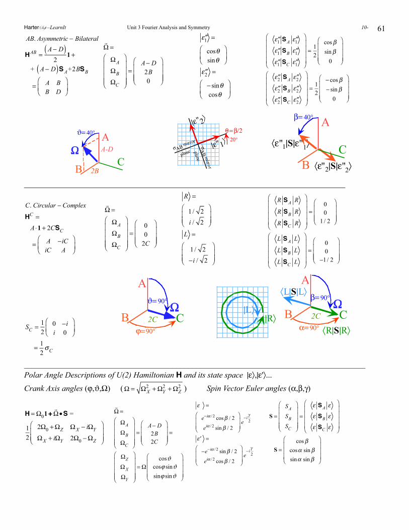
61
AB. Asymmetric − Bilateral
HAB =A− D( )
21 +
+ A− D( )SA+2BSB
= A BB D
⎛
⎝⎜⎞
⎠⎟
Ω =
ΩA
ΩB
ΩC
⎛
⎝
⎜⎜⎜⎜
⎞
⎠
⎟⎟⎟⎟
=A− D2B0
⎛
⎝
⎜⎜⎜
⎞
⎠
⎟⎟⎟
′′ε1 =
cosθsinθ
⎛
⎝⎜⎞
⎠⎟
′′ε2 =
− sinθcosθ
⎛
⎝⎜⎞
⎠⎟
′′ε1 SA ′′ε1
′′ε1 SB ′′ε1
′′ε1 SC ′′ε1
⎛
⎝
⎜⎜⎜⎜
⎞
⎠
⎟⎟⎟⎟
= 12
cosβsinβ
0
⎛
⎝
⎜⎜⎜
⎞
⎠
⎟⎟⎟
′′ε2 SA ′′ε2
′′ε2 SB ′′ε2
′′ε2 SC ′′ε2
⎛
⎝
⎜⎜⎜⎜
⎞
⎠
⎟⎟⎟⎟
= 12
− cosβ− sinβ
0
⎛
⎝
⎜⎜⎜
⎞
⎠
⎟⎟⎟
B
A
CΩ A-D
2B
ϑ= 40°
−σΑ
B mirro r
p la ne
σΑB mirror
plane
|ε" 2〉
|ε" 1〉θ = β/2
20°
〈ε"2|S|ε"2〉B
〈ε"1|S|ε"1〉
A
C
β= 40°
________________________________________________________________________________
C. Circular − Complex
HC =
A ⋅1 + 2CSC
= A −iCiC A
⎛
⎝⎜⎞
⎠⎟
Ω =
ΩA
ΩB
ΩC
⎛
⎝
⎜⎜⎜⎜
⎞
⎠
⎟⎟⎟⎟
=00
2C
⎛
⎝
⎜⎜⎜
⎞
⎠
⎟⎟⎟
R =
1 / 2i / 2
⎛
⎝⎜⎜
⎞
⎠⎟⎟
L =
1 / 2−i / 2
⎛
⎝⎜⎜
⎞
⎠⎟⎟
R SA R
R SB R
R SC R
⎛
⎝
⎜⎜⎜⎜
⎞
⎠
⎟⎟⎟⎟
=00
1 / 2
⎛
⎝
⎜⎜⎜
⎞
⎠
⎟⎟⎟
L SA L
L SB L
L SC L
⎛
⎝
⎜⎜⎜⎜
⎞
⎠
⎟⎟⎟⎟
=00
−1 / 2
⎛
⎝
⎜⎜⎜
⎞
⎠
⎟⎟⎟
SC = 12
0 −ii 0
⎛
⎝⎜⎞
⎠⎟
= 12σC
B
A
CΩ
2C
ϑ= 90°
ϕ= 90°
|R〉|L〉
B
A
CΩ
2C
β= 90°
α= 90° 〈R|S|R〉
〈L|S|L〉
_____________________________________________________________________________________Polar Angle Descriptions of U(2) Hamiltonian H and its state space |ε〉,|ε'〉...
Crank Axis angles (ϕ,ϑ,Ω) ( Ω = ΩX
2 +ΩY2 +ΩZ
2 ) Spin Vector Euler angles (α,β,γ)
H =Ω01+Ω•S =
12
2Ω0 +ΩZ ΩX − iΩY
ΩX + iΩY 2Ω0 −ΩZ
⎛
⎝⎜⎜
⎞
⎠⎟⎟
Ω =
ΩA
ΩB
ΩC
⎛
⎝
⎜⎜⎜⎜
⎞
⎠
⎟⎟⎟⎟
=A− D2B2C
⎛
⎝
⎜⎜⎜
⎞
⎠
⎟⎟⎟=
ΩZ
ΩX
ΩY
⎛
⎝
⎜⎜⎜⎜
⎞
⎠
⎟⎟⎟⎟
=Ωcosϑ
cosϕ sinϑsinϕ sinϑ
⎛
⎝
⎜⎜⎜
⎞
⎠
⎟⎟⎟
ε =
e−iα / 2 cosβ / 2
eiα / 2 sinβ / 2
⎛
⎝⎜⎜
⎞
⎠⎟⎟
e−iγ
2
′ε =
−e−iα / 2 sinβ / 2
eiα / 2 cosβ / 2
⎛
⎝⎜⎜
⎞
⎠⎟⎟
e−iγ
2
S =
SA
SB
SC
⎛
⎝
⎜⎜⎜⎜
⎞
⎠
⎟⎟⎟⎟
=
ε SA ε
ε SB ε
ε SC ε
⎛
⎝
⎜⎜⎜⎜
⎞
⎠
⎟⎟⎟⎟
S =cosβ
cosα sinβsinα sinβ
⎛
⎝
⎜⎜⎜
⎞
⎠
⎟⎟⎟
HarterSoft –LearnIt Unit 3 Fourier Analysis and Symmetry 10-
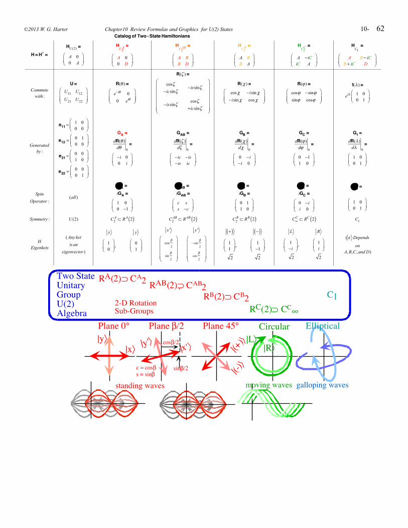
62
Catalog of Two -State Hamiltonians
H = H† =HU (2) =
A 00 A
⎛
⎝⎜⎞
⎠⎟
HC2
A =
A 00 D
⎛
⎝⎜⎞
⎠⎟
HC2
AB =
A BB D
⎛
⎝⎜⎞
⎠⎟
HC2
B =
A BB A
⎛
⎝⎜⎞
⎠⎟
HC2
C =
A −iCiC A
⎛
⎝⎜⎞
⎠⎟
HC1
=
A B − iCB + iC D
⎛
⎝⎜⎞
⎠⎟
Commutewith :
U =U11 U12
U21 U22
⎛
⎝⎜⎜
⎞
⎠⎟⎟
R(θ ) =
e−iθ 0
0 eiθ
⎛
⎝⎜⎜
⎞
⎠⎟⎟
R(ζ ) =
cosζ−icsinζ
−issinζ
−issinζcosζ
+icsinζ
⎛
⎝
⎜⎜⎜⎜⎜⎜
⎞
⎠
⎟⎟⎟⎟⎟⎟
R(χ ) =
cosχ −isinχ−isinχ cosχ
⎛
⎝⎜⎜
⎞
⎠⎟⎟
R(ϕ ) =
cosϕ −sinϕsinϕ cosϕ
⎛
⎝⎜⎜
⎞
⎠⎟⎟
1(λ) =
eiλ 1 00 1
⎛
⎝⎜⎞
⎠⎟
Generatedby :
e11 =1 00 0
⎛
⎝⎜⎞
⎠⎟
e12 = 0 10 0
⎛
⎝⎜⎞
⎠⎟
e21 =0 01 0
⎛
⎝⎜⎞
⎠⎟
e22 = 0 00 1
⎛
⎝⎜⎞
⎠⎟
GA =dR(θ )
dθ 0=
−i 00 i
⎛
⎝⎜⎞
⎠⎟
GAB =dR(ζ )
dζ 0=
−ic −is−is ic
⎛
⎝⎜⎞
⎠⎟
GB =dR(χ )
dχ 0=
0 −i−i 0
⎛
⎝⎜⎞
⎠⎟
GC =dR(ϕ )
dϕ 0=
0 −11 0
⎛
⎝⎜⎞
⎠⎟
G1 =dR(λ)
dλ 0=
1 00 1
⎛
⎝⎜⎞
⎠⎟
SpinOperator :
(all)
σA =iGA =
1 00 −1
⎛
⎝⎜⎞
⎠⎟
σAB =iGAB =
c ss −c
⎛
⎝⎜⎞
⎠⎟
σB =iGB =
0 11 0
⎛
⎝⎜⎞
⎠⎟
σC =iGC =
0 −ii 0
⎛
⎝⎜⎞
⎠⎟
σ0 =
1 00 1
⎛
⎝⎜⎞
⎠⎟
Symmetry : U (2) C2A ⊂ R A 2( ) C2
AB ⊂ R AB 2( ) C2B ⊂ RB 2( ) C∞
C ⊂ RC 2( ) C1
HEigenkets
( Any ketisan
eigenvector)
x
10
⎛
⎝⎜⎞
⎠⎟,
y
01
⎛
⎝⎜⎞
⎠⎟
x '
cosβ
2
sinβ
2
⎛
⎝
⎜⎜⎜⎜
⎞
⎠
⎟⎟⎟⎟
y '
− sinβ
2
cosβ
2
⎛
⎝
⎜⎜⎜⎜
⎞
⎠
⎟⎟⎟⎟
+( )11
⎛
⎝⎜⎞
⎠⎟,
2
−( )1−1
⎛
⎝⎜⎞
⎠⎟
2
L
1−i
⎛
⎝⎜⎞
⎠⎟,
2
R
1i
⎛
⎝⎜⎞
⎠⎟
2
( ε Depends
onA, B,C,and D)
|x〉|y〉
|x'〉|y'〉
|(-)〉
|(+)〉|L〉
|R〉
Plane 0° Plane β/2 Plane 45° Circular Elliptical
Two StateUnitaryGroupU(2)Algebra
RA(2)⊃ CA2 RAB(2)⊃ CAB2RB(2)⊃ CB2
RC(2)⊃ CC∞2-D RotationSub-Groups
C1
cosβ/2
standing waves moving waves galloping waves
sinβ/2c = cosβs = sinβ
©2013 W. G. Harter Chapter10 Review Formulas and Graphics for U(2) States 10-
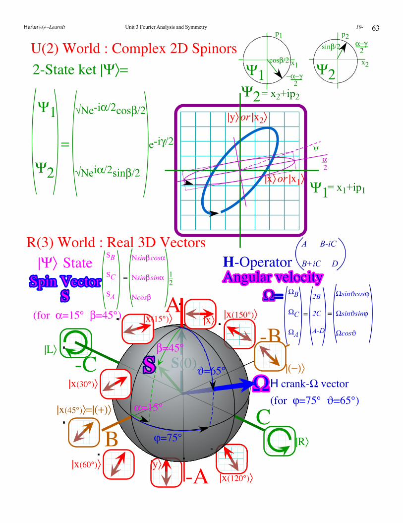
63
-B-C
|R〉
|L〉
|x(120°)〉
A
-A
CB
H crank-Ω vector(for ϕ=75° ϑ=65°)
|x(45°)〉=|(+)〉
|(−)〉
|x〉
|y〉
ΩΩ|x(30°)〉
|x(15°)〉
|x(60°)〉
|x(150°)〉
β=45°
ϑ=65°
ϕ=75°
α=15°
R(3) World : Real 3D Vectors
SS
H-OperatorAAnngguullaarr vveelloocciittyy
ΩΩ==
|Ψ〉 StateSSppiinn VVeeccttoorr
SS
Ψ1
Ψ2
2-State ket |Ψ〉=
Ψ1
Ψ2
=
√Ne-iα/2cosβ/2
e-iγ/2
√Neiα/2sinβ/2
U(2) World : Complex 2D SpinorsΨ2
α−γsinβ/2 2x2
p2
Ψ1 −α−γ
cosβ/2
2
x1
p1
= x2+ip2
= x1+ip1|x〉or |x1〉
|y〉or |x2〉
A B-iC
B+iC D
ΩB
ΩC
ΩA
2B
2C
A-D
Ωsinϑcosϕ
Ωsinϑsinϕ
Ωcosϑ
==
SB
SC
SA
Nsinβcosα
Nsinβ sinα
Ncosβ
=
(for α=15° β=45°)
12
α2
ψ
HarterSoft –LearnIt Unit 3 Fourier Analysis and Symmetry 10-
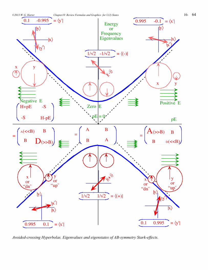
64
|x'〉|y'〉
|(+)〉
|(-)〉
|x'〉|y'〉
H+pE
H-pE
-S
-S
A(<<B)
D(>>B)
B
B=
A
A
B
B=
B=
D(<<B)
A(>>B) B
pE = 0
0.1 -0.995 = 〈y'| 0.995 -0.1 = 〈x'|
1/√2 -1/√2 = 〈(-)|
0.1 0.995 = 〈y'|0.995 0.1 = 〈x'|
1/√2 1/√2 = 〈(+)|
Energyor
FrequencyEigenvalues
pE
Positive ENegative EZero E
yor
“up”
|x〉
|y〉
xor
“dn”
|x〉
|y〉
|x〉
|y〉
|x〉
|y〉
yor
“up”
xor
“dn”
yx
yx
Avoided-crossing Hyperbolas. Eigenvalues and eigenstates of AB-symmetry Stark-effects.
©2013 W. G. Harter Chapter10 Review Formulas and Graphics for U(2) States 10-
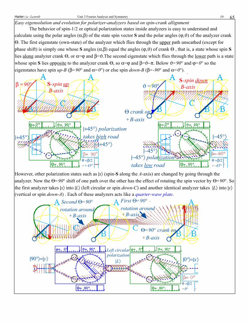
65Easy eigensolution and evolution for polarizer-analyzers based on spin-crank allignment The behavior of spin-1/2 or optical polarization states inside analyzers is easy to understand and calculate using the polar angles (α,β) of the state spin vector S and the polar angles (ϕ,ϑ) of the analyzer crank Θ. The first eigenstate (own-state) of the analyzer which flies through the upper path unscathed (except for phase shift) is simply one whose S angles (α,β) equal the angles (ϕ,ϑ) of crank Θ , that is, a state whose spin S lies along analyzer crank Θ, or α=ϕ and β=ϑ.The second eigenstate which flies through the lower path is a state whose spin S lies opposite to the analyzer crank Θ, so α=ϕ and β=ϑ−π. Below ϑ=90° and ϕ=0° so the eigenstates have spin up-B (β=90° and α=0°) or else spin down-B (β=-90° and α=0°).
S-spin up B-axis
|+45°〉 polarizationtakes high road
|+45°〉|+45°〉
β =90°
θ =β/2=+45°
Θ crank on +B-axis
S-spin down B-axis
|−45°〉 polarizationtakes low road
|−45°〉
|−45°〉
ϑ =90°
θ =β/2=-45°
However, other polarization states such as |x〉 (spin-S along the A-axis) are changed by going through the analyzer. Now the Θ=90° shift of one path over the other has the effect of rotating the spin vector by Θ=90°. So the first analyzer takes |x〉 into |L〉 (left circular or spin down-C) and another identical analyzer takes |L〉 into |y〉 (vertical or spin down-A) . Each of these analyzers acts like a quarter-wave plate.
|0°〉=|x〉|90°〉=|y〉
Left circularpolarization
|L〉
Θ=90° crank on +B-axis
Second Θ=90°rotation around
+B-axis
First Θ=90°rotation around +B-axis
θ =β/2=0°
HarterSoft –LearnIt Unit 3 Fourier Analysis and Symmetry 10-
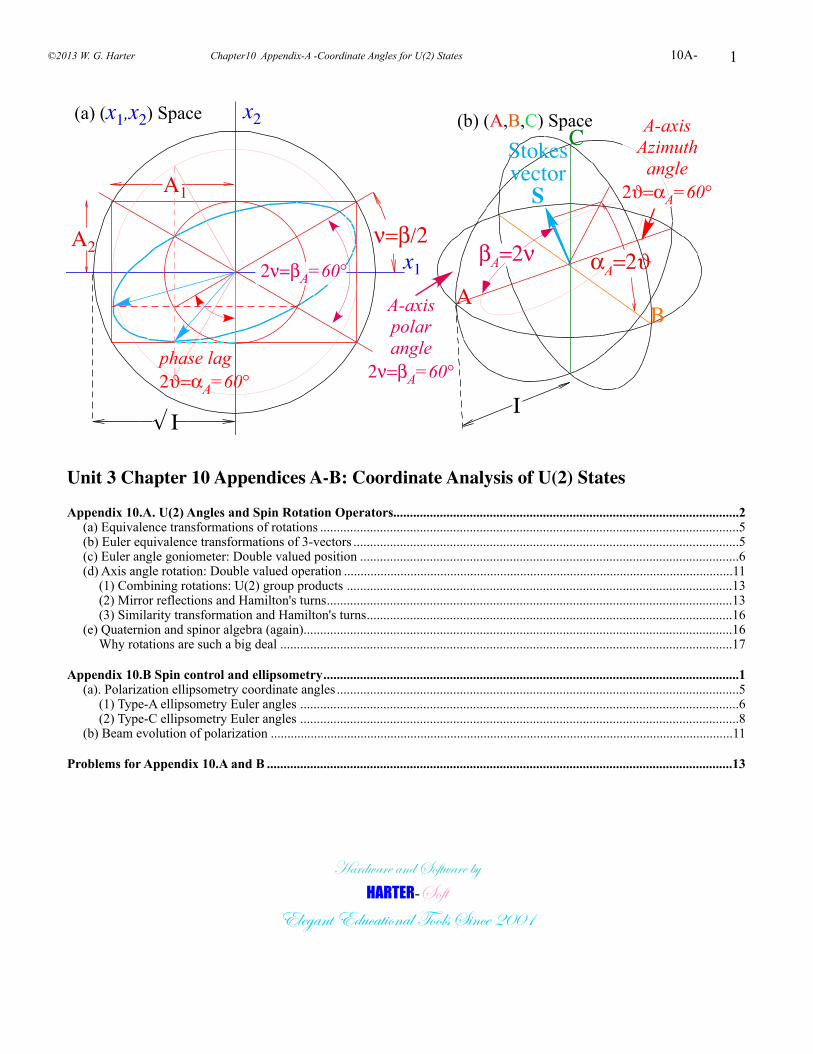
1
x1
x2
√ I
ν=β/2
A1
I
AB
C
βA=2ν αA=2ϑA2
(a) (x1,x2) Space (b) (A,B,C) Space
A-axispolarangle
2ν=βA=60°
StokesvectorS
A-axisAzimuthangle
2ϑ=αA=60°
phase lag2ϑ=αA=60°
2ν=βA=60°
Unit 3 Chapter 10 Appendices A-B: Coordinate Analysis of U(2) States
........................................................................................................Appendix 10.A. U(2) Angles and Spin Rotation Operators 2..............................................................................................................................(a) Equivalence transformations of rotations 5
....................................................................................................................(b) Euler equivalence transformations of 3-vectors 5..................................................................................................................(c) Euler angle goniometer: Double valued position 6
.....................................................................................................................(d) Axis angle rotation: Double valued operation 11....................................................................................................................(1) Combining rotations: U(2) group products 13
..........................................................................................................................(2) Mirror reflections and Hamilton's turns 13..............................................................................................................(3) Similarity transformation and Hamilton's turns 16
.................................................................................................................................(e) Quaternion and spinor algebra (again) 16........................................................................................................................................Why rotations are such a big deal 17
.............................................................................................................................Appendix 10.B Spin control and ellipsometry 1.........................................................................................................................(a). Polarization ellipsometry coordinate angles 5
....................................................................................................................................(1) Type-A ellipsometry Euler angles 6
....................................................................................................................................(2) Type-C ellipsometry Euler angles 8...........................................................................................................................................(b) Beam evolution of polarization 11
............................................................................................................................................Problems for Appendix 10.A and B 13
Hardware and Software by HARTER-Soft
Elegant Educational Tools Since 2001
©2013 W. G. Harter Chapter10 Appendix-A -Coordinate Angles for U(2) States 10A-
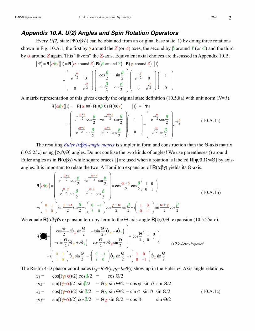
2
Appendix 10.A. U(2) Angles and Spin Rotation Operators Every U(2) state |Ψ(αβγ)〉 can be obtained from an original base state |1〉 by doing three rotations shown in Fig. 10.A.1, the first by γ around the Z (or A) axes, the second by β around Y (or C) and the third by α around Z again. This “favors” the Z-axis. Equivalent axial choices are discussed in Appendix 10.B.
Ψ =R αβγ( ) 1 =R α around Z( ) R β around Y( ) R γ around Z( ) 1
= e−iα
2 0
0 eiα2
⎛
⎝
⎜⎜⎜
⎞
⎠
⎟⎟⎟
cos
β2
−sinβ2
sinβ2
cosβ2
⎛
⎝
⎜⎜⎜⎜
⎞
⎠
⎟⎟⎟⎟
e−iγ
2 0
0 eiγ2
⎛
⎝
⎜⎜⎜
⎞
⎠
⎟⎟⎟
1
0
⎛
⎝
⎜⎜⎜
⎞
⎠
⎟⎟⎟
A matrix representation of this gives exactly the original state definition (10.5.8a) with unit norm (N=1).
R αβγ( ) 1 = R α 00( ) R 0β 0( ) R 00γ( ) 1 = Ψ
=e−iα+γ
2 cosβ2
−e−iα−γ
2 sinβ2
eiα−γ
2 sinβ2
eiα+γ
2 cosβ2
⎛
⎝
⎜⎜⎜⎜⎜
⎞
⎠
⎟⎟⎟⎟⎟
1
0
⎛
⎝
⎜⎜⎜
⎞
⎠
⎟⎟⎟=
e−iα
2 cosβ2
eiα2 sin
β2
⎛
⎝
⎜⎜⎜⎜⎜
⎞
⎠
⎟⎟⎟⎟⎟
e−iγ
2 (10.A.1a)
The resulting Euler (αβγ)-angle matrix is simpler in form and construction than the Θ-axis matrix (10.5.25c) using [ϕ,ϑ,Θ] angles. Do not confuse the two kinds of angles! We use parentheses () around Euler angles as in R(αβγ) while square braces [] are used when a rotation is labeled R[ϕ,ϑ,Ωt=Θ] by axis-angles. It is important to relate the two. A Hamilton expansion of R(αβγ) yields its Θ-axis.
R αβγ( ) =e−iα+γ
2 cosβ2
−e−iα−γ
2 sinβ2
eiα−γ
2 sinβ2
eiα+γ
2 cosβ2
⎛
⎝
⎜⎜⎜⎜⎜
⎞
⎠
⎟⎟⎟⎟⎟
= cosα + γ
2cos
β2
1 00 1
⎛
⎝⎜⎞
⎠⎟
−i 0 11 0
⎛
⎝⎜⎞
⎠⎟sin
γ −α2
sinβ2− i 0 −i
i 0
⎛
⎝⎜⎞
⎠⎟cos
γ −α2
sinβ2− i 1 0
0 −1
⎛
⎝⎜⎞
⎠⎟sin
α + γ2
cosβ2
(10.A.1b)
We equate R(αβγ)'s expansion term-by-term to the Θ-axis-angle R[ϕ,ϑ,Θ] expansion (10.5.25a-c).
RΘ⎡⎣ ⎤⎦=
cosΘ2− iΘZ sin
Θ2
−isinΘ2
ΘX − iΘY( )−isinΘ
2ΘX + iΘY( ) cos
Θ2+ iΘZ sin
Θ2
⎛
⎝
⎜⎜⎜⎜
⎞
⎠
⎟⎟⎟⎟
= cosΘ2
1 00 1
⎛
⎝⎜⎞
⎠⎟
− i 0 11 0
⎛
⎝⎜⎞
⎠⎟ΘX sin
Θ2
− i 0 −ii 0
⎛
⎝⎜⎞
⎠⎟ΘY sin
Θ2
− i 1 00 −1
⎛
⎝⎜⎞
⎠⎟ΘZ sin
Θ2
(10.5.25a-c)repeated
The Re-Im 4-D phasor coordinates (xj=ReΨj, pj=ImΨj) show up in the Euler vs. Axis angle relations. x1 = cos[(γ+α)/2] cosβ/2 = cos Θ/2 -p2= sin[(γ−α)/2] sinβ/2 = Θ X sin Θ/2 = cos ϕ sin ϑ sin Θ/2 x2 = cos[(γ−α)/2] sinβ/2 = Θ Y sin Θ/2 = sin ϕ sin ϑ sin Θ/2 (10.A.1c) -p1= sin[(γ+α)/2] cosβ/2 = Θ Z sin Θ/2 = cos ϑ sin Θ/2
HarterSoft –LearnIt Unit 3 Fourier Analysis and Symmetry 10-A
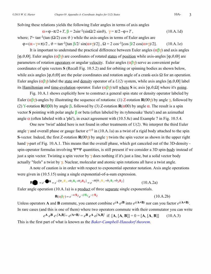
3
Solving these relations yields the following Euler angles in terms of axis angles α = ϕ −π/2 + T, β = 2sin-1(sinΩ/2 sinϑ), γ = π/2 −ϕ + T , (10.A.1d)where; T= tan-1(tan (Ω/2) cos ϑ ) while the axis-angles in terms of Euler angles are ϕ = (α − γ + π)/2 , ϑ = tan-1[tan β/2/ sin(α+γ)/2] , Ω = 2 cos-1[cos β/2 cos(α+γ)/2].: (10.A.1e) It is important to understand the practical difference between Euler angles (αβγ) and axis angles [ϕ,ϑ,Θ]. Euler angles (αβγ) are coordinates of rotated states of position while axis-angles [ϕ,ϑ,Θ] are parameters of rotation operators or angular velocity. Euler angles (αβγ) serve as convenient polar coordinates of spin vectors S (Recall Fig. 10.5.2) and for orbiting or spinning bodies as shown below, while axis angles [ϕ,ϑ,Θ] are the polar coordinates and rotation angle of a crank-axis Ω for an operation. Euler angles (αβγ) label the state and density operator of a U(2) system, while axis angles [ϕ,ϑ,Θ] label its Hamiltonian and time-evolution operator. Euler (αβγ) tell where S is; axis [ϕ,ϑ,Ω] where it's going. Fig. 10.A.1 shows explicitly how to construct a general spin state or density operator labeled by Euler (αβγ)-angles by illustrating the sequence of rotations: (1) Z-rotation R(00γ) by angle γ, followed by (2) Y-rotation R(0β0) by angle β, followed by (3) Z-rotation R(α00) by angle α. The result is a spin vector S pointing with polar angle β or beta (often labeled by its ryhmesake 'theta') and an azimuthal angle α (often labeled with a 'phi'), in exact agreement with (10.5.8c) and Example 7 in Fig. 10.5.4. One new 'twist' added here is not found in other treatments of U(2). We interpret the third Euler angle γ and overall phase or gauge factor e-iγ/2 in (10.A.1a) as a twist of a rigid body attached to the spin S-vector. Indeed, the first Z-rotation R(00γ) by angle γ twists the spin vector as shown in the upper right hand γ-part of Fig. 10.A.1. This means that the overall phase, which got canceled out of the 3D-density -spin-operator formulas involving Ψ*Ψ quantities, is still present if we consider a 3D spin-body instead of just a spin vector. Twisting a spin vector by γ does nothing if it's just a line, but a solid vector body actually "feels" a twist by γ. Nuclear, molecular and atomic spin rotations all have a twist angle. A note of caution is in order with respect to exponential operator notation. Axis angle operations were given in (10.5.15) using a single exponential-of-a-sum expression.
R[Θ] = e−i
Θ•S = e−i ΘXSX +ΘYSY +ΘZSZ( ) = e−iΘ ΘXSX +ΘYSY +ΘZSZ( ) (10.A.2a)
Euler angle operation (10.A.1a) is a product of three separate single exponentials.
R(αβγ ) = e−iαSZ e−iβSY e−iγ SZ (10.A.2b)
Unless operators A and B commute, you cannot combine eiA eiB into ei(A+B) nor can you factor ei(A+B). In rare cases (and this is one of them) where two operators commute with their commutator you can write eA eB e-[A,B]= e(A+B) = eB eA e[A,B] if: [A, [A, B]] = 0 = [A, [A, B]] (10.A.3)This is the first part of what is known as the Baker-Campbell-Hausdorf theorem.
©2013 W. G. Harter Chapter10 Appendix-A -Coordinate Angles for U(2) States 10A-
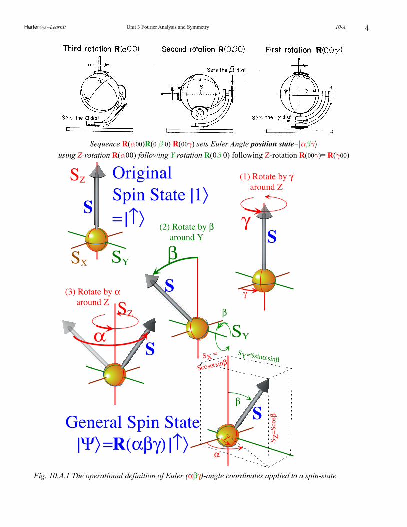
4
Sequence R(α00)R(0 β 0) R(00γ) sets Euler Angle position state-⏐αβγ〉
using Z-rotation R(α00) following Y-rotation R(0β 0) following Z-rotation R(00γ)= R(γ00)
S
SYSXS
SZ
S
S
SZ
S
(1) Rotate by γaround Z
β
γ
(2) Rotate by βaround Y
(3) Rotate by αaround Z
γ
αβ
OriginalSpin State |1〉= |↑〉
General Spin State|Ψ〉=R(αβγ) |↑〉
β
α
SY=Ssinα sinβ
S Z=Scosβ
SX=
Scosα sinβ
SY
γ
Fig. 10.A.1 The operational definition of Euler (αβγ)-angle coordinates applied to a spin-state.
HarterSoft –LearnIt Unit 3 Fourier Analysis and Symmetry 10-A
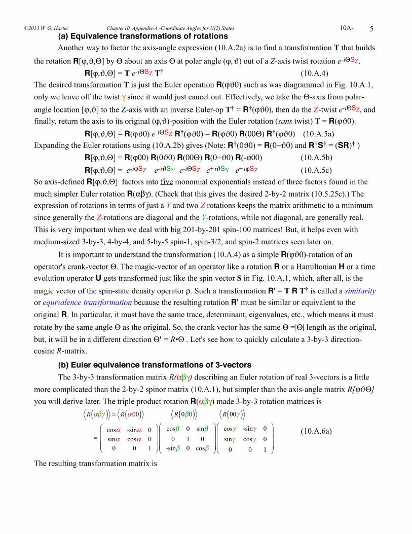
5! (a) Equivalence transformations of rotations Another way to factor the axis-angle expression (10.A.2a) is to find a transformation T that builds
the rotation R[ϕ,ϑ,Θ] by Θ about an axis Θ at polar angle (ϕ, ϑ) out of a Z-axis twist rotation e-iΘSZ. R[ϕ,ϑ,Θ] = T e-iΘSZ T† (10.A.4)The desired transformation T is just the Euler operation R(ϕϑ0) such as was diagrammed in Fig. 10.A.1, only we leave off the twist γ since it would just cancel out. Effectively, we take the Θ-axis from polar-angle location [ϕ,ϑ] to the Z-axis with an inverse Euler-op T† = R†(ϕϑ0), then do the Z-twist e-iΘSZ, and finally, return the axis to its original (ϕ,ϑ)-position with the Euler rotation (sans twist) T = R(ϕϑ0). R[ϕ,ϑ,Θ] = R(ϕϑ0) e-iΘSZ R†(ϕϑ0) = R(ϕϑ0) R(00Θ) R†(ϕϑ0) (10.A.5a) Expanding the Euler rotations using (10.A.2b) gives (Note: R†(0ϑ0) = R(0−ϑ0) and R†S† = (SR)† ) R[ϕ,ϑ,Θ] = R(ϕ00) R(0ϑ0) R(00Θ) R(0−ϑ0) R(-ϕ00) (10.A.5b) R[ϕ,ϑ,Θ] = e-iϕSZ e-iϑSY e-iΘSZ e+iϑSY e+iϕSZ (10.A.5c)So axis-defined R[ϕ,ϑ,Θ] factors into five monomial exponentials instead of three factors found in the much simpler Euler rotation R(αβγ). (Check that this gives the desired 2-by-2 matrix (10.5.25c).) The expression of rotations in terms of just a Y and two Z rotations keeps the matrix arithmetic to a minimum since generally the Z-rotations are diagonal and the Y-rotations, while not diagonal, are generally real. This is very important when we deal with big 201-by-201 spin-100 matrices! But, it helps even with medium-sized 3-by-3, 4-by-4, and 5-by-5 spin-1, spin-3/2, and spin-2 matrices seen later on. It is important to understand the transformation (10.A.4) as a simple R(ϕϑ0)-rotation of an operator's crank-vector Θ. The magic-vector of an operator like a rotation R or a Hamiltonian H or a time evolution operator U gets transformed just like the spin vector S in Fig. 10.A.1, which, after all, is the magic vector of the spin-state density operator ρ. Such a transformation R' = T R T† is called a similarity or equivalence transformation because the resulting rotation R' must be similar or equivalent to the original R. In particular, it must have the same trace, determinant, eigenvalues, etc., which means it must rotate by the same angle Θ as the original. So, the crank vector has the same Θ =|Θ| length as the original, but, it will be in a different direction Θ' = R•Θ . Let's see how to quickly calculate a 3-by-3 direction-cosine R-matrix.
! (b) Euler equivalence transformations of 3-vectors The 3-by-3 transformation matrix R(αβγ) describing an Euler rotation of real 3-vectors is a little more complicated than the 2-by-2 spinor matrix (10.A.1), but simpler than the axis-angle matrix R[ϕϑΘ] you will derive later. The triple product rotation R(αβγ) made 3-by-3 rotation matrices is
R αβγ( ) = R α00( ) R 0β0( ) R 00γ( )
= cosα -sinα 0sinα cosα 0
0 0 1
⎛
⎝
⎜⎜⎜
⎞
⎠
⎟⎟⎟
cosβ 0 sinβ0 1 0
-sinβ 0 cosβ
⎛
⎝
⎜⎜⎜
⎞
⎠
⎟⎟⎟
cosγ -sinγ 0
sinγ cosγ 0
0 0 1
⎛
⎝
⎜⎜⎜
⎞
⎠
⎟⎟⎟
(10.A.6a)
The resulting transformation matrix is
©2013 W. G. Harter Chapter10 Appendix-A -Coordinate Angles for U(2) States 10A-
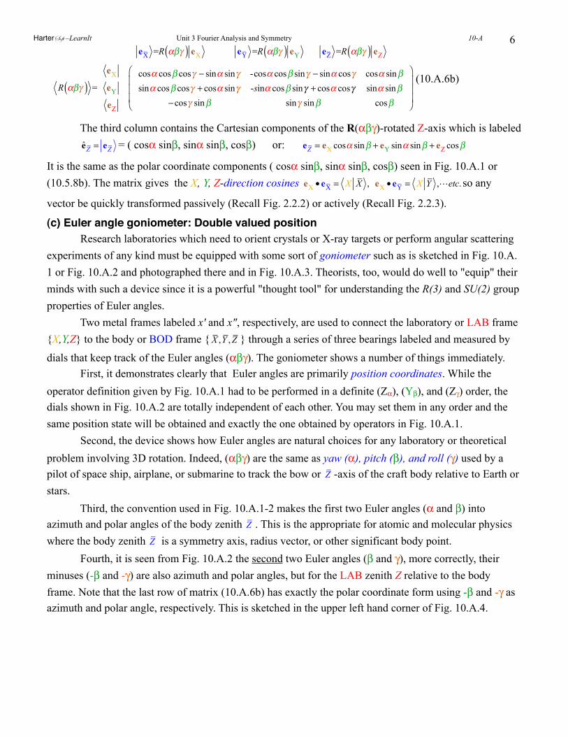
6
eX =R αβγ( ) eX eY =R αβγ( ) eY eZ =R αβγ( ) eZ
R αβγ( ) =
eX
eY
eZ
cosα cosβ cosγ − sinα sinγ -cosα cosβ sinγ − sinα cosγ cosα sinβsinα cosβ cosγ + cosα sinγ -sinα cosβ sinγ + cosα cosγ sinα sinβ
−cosγ sinβ sinγ sinβ cosβ
⎛
⎝
⎜⎜⎜
⎞
⎠
⎟⎟⎟
(10.A.6b)
The third column contains the Cartesian components of the R(αβγ)-rotated Z-axis which is labeled
eZ = eZ = ( cosα sinβ, sinα sinβ, cosβ) or: eZ = eX cosα sinβ + eY sinα sinβ + eZ cosβ
It is the same as the polar coordinate components ( cosα sinβ, sinα sinβ, cosβ) seen in Fig. 10.A.1 or (10.5.8b). The matrix gives the X, Y, Z-direction cosines
eX • eX = X X , eX • eY = X Y ,etc. so any
vector be quickly transformed passively (Recall Fig. 2.2.2) or actively (Recall Fig. 2.2.3).
(c) Euler angle goniometer: Double valued position Research laboratories which need to orient crystals or X-ray targets or perform angular scattering experiments of any kind must be equipped with some sort of goniometer such as is sketched in Fig. 10.A.1 or Fig. 10.A.2 and photographed there and in Fig. 10.A.3. Theorists, too, would do well to "equip" their minds with such a device since it is a powerful "thought tool" for understanding the R(3) and SU(2) group properties of Euler angles. Two metal frames labeled x' and x", respectively, are used to connect the laboratory or LAB frame {X,Y,Z} to the body or BOD frame { X ,Y , Z } through a series of three bearings labeled and measured by
dials that keep track of the Euler angles (αβγ). The goniometer shows a number of things immediately. First, it demonstrates clearly that Euler angles are primarily position coordinates. While the operator definition given by Fig. 10.A.1 had to be performed in a definite (Zα), (Yβ), and (Zγ) order, the dials shown in Fig. 10.A.2 are totally independent of each other. You may set them in any order and the same position state will be obtained and exactly the one obtained by operators in Fig. 10.A.1. Second, the device shows how Euler angles are natural choices for any laboratory or theoretical problem involving 3D rotation. Indeed, (αβγ) are the same as yaw (α), pitch (β), and roll (γ) used by a pilot of space ship, airplane, or submarine to track the bow or Z -axis of the craft body relative to Earth or stars. Third, the convention used in Fig. 10.A.1-2 makes the first two Euler angles (α and β) into azimuth and polar angles of the body zenith Z . This is the appropriate for atomic and molecular physics where the body zenith Z is a symmetry axis, radius vector, or other significant body point. Fourth, it is seen from Fig. 10.A.2 the second two Euler angles (β and γ), more correctly, their minuses (-β and -γ) are also azimuth and polar angles, but for the LAB zenith Z relative to the body frame. Note that the last row of matrix (10.A.6b) has exactly the polar coordinate form using -β and -γ as azimuth and polar angle, respectively. This is sketched in the upper left hand corner of Fig. 10.A.4.
HarterSoft –LearnIt Unit 3 Fourier Analysis and Symmetry 10-A
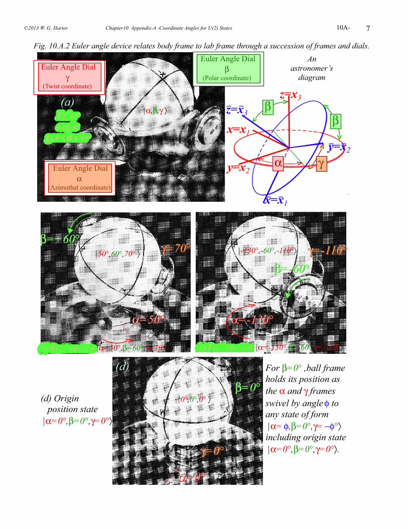
7
Fig. 10.A.2 Euler angle device relates body frame to lab frame through a succession of frames and dials.
((bb)) PPoossiittiioonn ssttaattee |α=50°,β=60°,γ=70°〉〉〉 ((cc)) PPoossiittiioonn ssttaattee |α=-130°,β=-60°,γ=-110°〉
β=+60°γ=70°
α=50°α=50°
β=+60°
β=-60°β=-60°
γ=70° γ=-110°γ=-110°
α=-130°α=-130°
|50°,60°,70° 〉 |-130°,-60°,-110°〉
(d) Originposition state|α=0°,β=0°,γ=0°〉
For β=0° ,ball frameholds its position asthe α and γ framesswivel by angleφ toany state of form|α=φ,β=0°,γ=−φ°〉including origin state|α=0°,β=0°,γ=0°〉.
α=0°α=0°
γ=0°γ=0°
β=0°β=0°|0°,0°,0° 〉
(d)
EEuulleerraannggllee
ggoonniioommeetteerr
Euler Angle Dialγ
(Twist coordinate)
Euler Angle Dialα
(Azimuthal coordinate)
(a)|α,β,γ 〉 β
α γ
βx=x1
y=x2
z=x3
x=x1
y=x2
z=x3
Anastronomer’sdiagram
Euler Angle Dialβ
(Polar coordinate)
©2013 W. G. Harter Chapter10 Appendix-A -Coordinate Angles for U(2) States 10A-
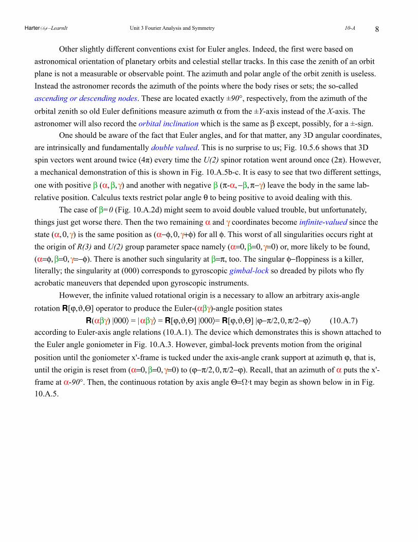
8
Other slightly different conventions exist for Euler angles. Indeed, the first were based on astronomical orientation of planetary orbits and celestial stellar tracks. In this case the zenith of an orbit plane is not a measurable or observable point. The azimuth and polar angle of the orbit zenith is useless. Instead the astronomer records the azimuth of the points where the body rises or sets; the so-called ascending or descending nodes. These are located exactly ±90°, respectively, from the azimuth of the orbital zenith so old Euler definitions measure azimuth α from the ±Y-axis instead of the X-axis. The astronomer will also record the orbital inclination which is the same as β except, possibly, for a ±-sign. One should be aware of the fact that Euler angles, and for that matter, any 3D angular coordinates, are intrinsically and fundamentally double valued. This is no surprise to us; Fig. 10.5.6 shows that 3D spin vectors went around twice (4π) every time the U(2) spinor rotation went around once (2π). However, a mechanical demonstration of this is shown in Fig. 10.A.5b-c. It is easy to see that two different settings, one with positive β (α, β, γ) and another with negative β (π-α, −β, π−γ) leave the body in the same lab-relative position. Calculus texts restrict polar angle θ to being positive to avoid dealing with this. The case of β=0 (Fig. 10.A.2d) might seem to avoid double valued trouble, but unfortunately, things just get worse there. Then the two remaining α and γ coordinates become infinite-valued since the state (α, 0, γ) is the same position as (α−φ, 0, γ+φ) for all φ. This worst of all singularities occurs right at the origin of R(3) and U(2) group parameter space namely (α=0, β=0, γ=0) or, more likely to be found, (α=φ, β=0, γ=−φ). There is another such singularity at β=π, too. The singular φ−floppiness is a killer, literally; the singularity at (000) corresponds to gyroscopic gimbal-lock so dreaded by pilots who fly acrobatic maneuvers that depended upon gyroscopic instruments. However, the infinite valued rotational origin is a necessary to allow an arbitrary axis-angle rotation R[ϕ,ϑ,Θ] operator to produce the Euler-(αβγ)-angle position states R(αβγ) |000〉 = | αβγ〉 = R[ϕ,ϑ,Θ] |000〉= R[ϕ,ϑ,Θ] |ϕ−π/2, 0, π/2−ϕ〉 (10.A.7)according to Euler-axis angle relations (10.A.1). The device which demonstrates this is shown attached to the Euler angle goniometer in Fig. 10.A.3. However, gimbal-lock prevents motion from the original position until the goniometer x'-frame is tucked under the axis-angle crank support at azimuth ϕ, that is, until the origin is reset from (α=0, β=0, γ=0) to (ϕ−π/2, 0, π/2−ϕ). Recall, that an azimuth of α puts the x'-frame at α-90°. Then, the continuous rotation by axis angle Θ=Ω·t may begin as shown below in in Fig. 10.A.5.
HarterSoft –LearnIt Unit 3 Fourier Analysis and Symmetry 10-A
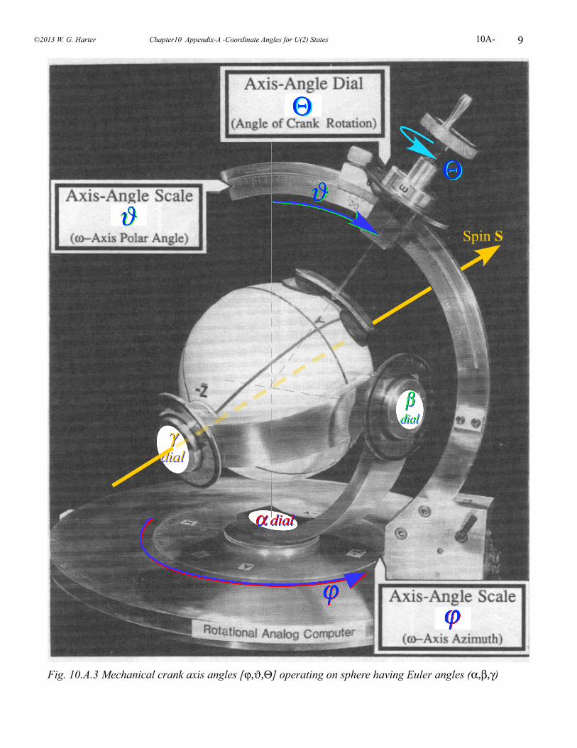
9
Spin S
Fig. 10.A.3 Mechanical crank axis angles [ϕ,ϑ,Θ] operating on sphere having Euler angles (α,β,γ)
©2013 W. G. Harter Chapter10 Appendix-A -Coordinate Angles for U(2) States 10A-
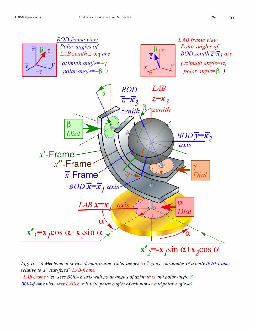
10
BOD frame viewz
x y
−β
−γ
Polar angles ofLAB zenith z=x3 are(azimuth angle=−γ,polar angle=−β )
zLAB frame view
α
Polar angles ofBOD zenith z=x3 are(azimuth angle=α,polar angle=β )
z
x yzβ
LAB x=x1 axisαDial
LABz=x3zenith
BODz=x3zenith
βDial
γDial
BOD y=x2axis
BOD x=x1 axis
αα
β
β
γ
γ
x′-Framex′′-Frame
x′′1=x1cos α+x2sin α
x′′2=-x1sin α+x2cos α
x-Frame
Fig. 10.A.4 Mechanical device demonstrating Euler angles (α,β,γ) as coordinates of a body BOD-frame relative to a “star-fixed” LAB-frame. LAB-frame view sees BOD-Z axis with polar angles of azimuth α and polar angle β.BOD-frame view sees LAB-Z axis with polar angles of azimuth -γ and polar angle -β.
HarterSoft –LearnIt Unit 3 Fourier Analysis and Symmetry 10-A
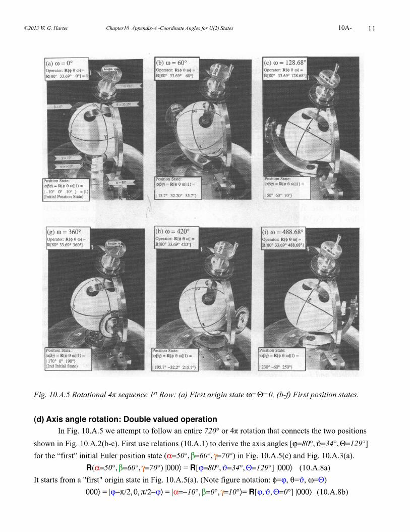
11
Fig. 10.A.5 Rotational 4π sequence 1st Row: (a) First origin state ω=Θ=0, (b-f) First position states.
!(d) Axis angle rotation: Double valued operation In Fig. 10.A.5 we attempt to follow an entire 720° or 4π rotation that connects the two positions shown in Fig. 10.A.2(b-c). First use relations (10.A.1) to derive the axis angles [ϕ=80°, ϑ=34°, Θ=129°] for the “first” initial Euler position state (α=50°, β=60°, γ=70°) in Fig. 10.A.5(c) and Fig. 10.A.3(a). R(α=50°, β=60°, γ=70°) |000〉 = R[ϕ=80°, ϑ=34°, Θ=129°] |000〉 (10.A.8a)It starts from a "first" origin state in Fig. 10.A.5(a). (Note figure notation: φ=ϕ, θ=ϑ, ω=Θ) |000〉 = |ϕ−π/2, 0, π/2−ϕ〉 = |α=−10°, β=0°, γ=10°〉= R[ϕ, ϑ, Θ=0°] |000〉 (10.A.8b)
©2013 W. G. Harter Chapter10 Appendix-A -Coordinate Angles for U(2) States 10A-
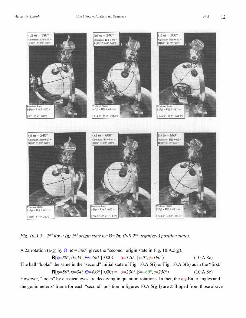
12
Fig. 10.A.5 2nd Row: (g) 2nd origin state ω=Θ=2π, (h-l) 2nd negative-β position states.
A 2π rotation (a-g) by Θ=ω = 360° gives the "second" origin state in Fig. 10.A.5(g). R[ϕ=80°, ϑ=34°, Θ=360°] |000〉 = |α=170°, β=0°, γ=190°〉 (10.A.8c) The ball “looks” the same in the "second" initial state of Fig. 10.A.5(i) or Fig. 10.A.3(b) as in the “first.” R[ϕ=80°, ϑ=34°, Θ=489°] |000〉 = |α=230°, β=−60°, γ=250°〉 (10.A.8c) However, “looks” by classical eyes are deceiving in quantum rotations. In fact, the α,γ-Euler angles and the goniometer x'-frame for each “second” position in figures 10.A.5(g-l) are π-flipped from those above
HarterSoft –LearnIt Unit 3 Fourier Analysis and Symmetry 10-A
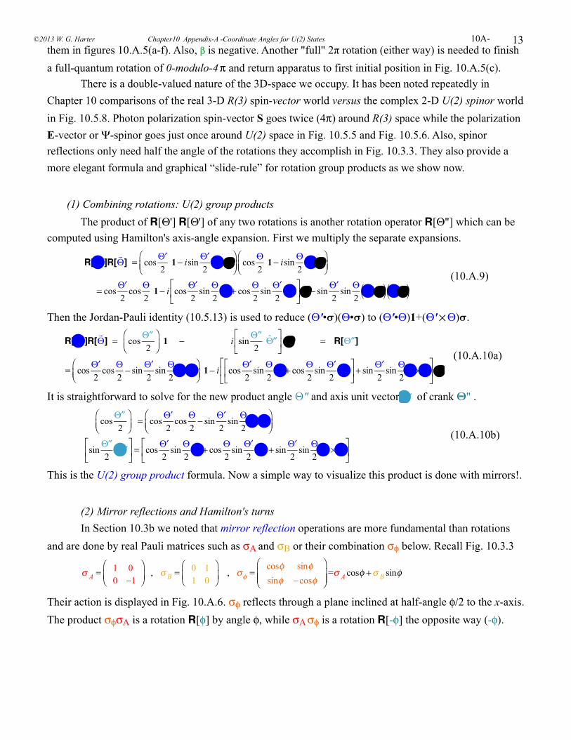
13them in figures 10.A.5(a-f). Also, β is negative. Another "full" 2π rotation (either way) is needed to finish a full-quantum rotation of 0-modulo-4 π and return apparatus to first initial position in Fig. 10.A.5(c). There is a double-valued nature of the 3D-space we occupy. It has been noted repeatedly in Chapter 10 comparisons of the real 3-D R(3) spin-vector world versus the complex 2-D U(2) spinor world in Fig. 10.5.8. Photon polarization spin-vector S goes twice (4π) around R(3) space while the polarization E-vector or Ψ-spinor goes just once around U(2) space in Fig. 10.5.5 and Fig. 10.5.6. Also, spinor reflections only need half the angle of the rotations they accomplish in Fig. 10.3.3. They also provide a more elegant formula and graphical “slide-rule” for rotation group products as we show now.
(1) Combining rotations: U(2) group products The product of R[Θ'] R[Θ'] of any two rotations is another rotation operator R[Θ"] which can be computed using Hamilton's axis-angle expansion. First we multiply the separate expansions.
R[ ′Θ ]R[
Θ] = cos
′Θ2
1− isin ′Θ2
′Θ iσ⎛⎝⎜
⎞⎠⎟
cosΘ2
1− isinΘ2
Θiσ⎛⎝⎜
⎞⎠⎟
= cos′Θ
2cos
Θ2
1− i cos′Θ
2sin
Θ2
Θ + cosΘ2
sin′Θ
2 ′Θ
⎡
⎣⎢
⎤
⎦⎥iσ − sin
′Θ2
sinΘ2
′Θ iσ( ) Θiσ( ) (10.A.9)
Then the Jordan-Pauli identity (10.5.13) is used to reduce (Θ'•σ)(Θ•σ) to (Θ'•Θ)1+(Θ'×Θ)σ.
R[ ′Θ ]R[
Θ] = cos
′′Θ2
⎛⎝⎜
⎞⎠⎟
1 − i sin′′Θ
2 ′′Θ
⎡
⎣⎢
⎤
⎦⎥ iσ = R[ ′′Θ ]
= cos′Θ
2cos
Θ2− sin
′Θ2
sinΘ2
′Θ iΘ⎛⎝⎜
⎞⎠⎟
1− i cos′Θ
2sin
Θ2
Θ + cosΘ2
sin′Θ
2 ′Θ
⎡
⎣⎢
⎤
⎦⎥ + sin
′Θ2
sinΘ2
′Θ ×Θ⎡
⎣⎢
⎤
⎦⎥iσ
(10.A.10a)
It is straightforward to solve for the new product angle Θ" and axis unit vector ′′Θ of crank Θ" .
cos′′Θ
2⎛⎝⎜
⎞⎠⎟
= cos′Θ
2cos
Θ2− sin
′Θ2
sinΘ2
′Θ iΘ⎛⎝⎜
⎞⎠⎟
sin′′Θ
2 ′′Θ
⎡
⎣⎢
⎤
⎦⎥ = cos
′Θ2
sinΘ2
Θ + cosΘ2
sin′Θ
2 ′Θ + sin
′Θ2
sinΘ2
′Θ × Θ⎡
⎣⎢
⎤
⎦⎥
(10.A.10b)
This is the U(2) group product formula. Now a simple way to visualize this product is done with mirrors!.
(2) Mirror reflections and Hamilton's turns In Section 10.3b we noted that mirror reflection operations are more fundamental than rotations and are done by real Pauli matrices such as σA and σB or their combination σφ below. Recall Fig. 10.3.3
σ A = 1 0
0 −1
⎛
⎝⎜⎞
⎠⎟ , σ B = 0 1
1 0
⎛
⎝⎜⎞
⎠⎟ , σφ =
cosφ sinφsinφ −cosφ
⎛
⎝⎜⎜
⎞
⎠⎟⎟
=σ A cosφ +σ B sinφ
Their action is displayed in Fig. 10.A.6. σφ reflects through a plane inclined at half-angle φ/2 to the x-axis. The product σφσA is a rotation R[φ] by angle φ, while σA σφ is a rotation R[-φ] the opposite way (-φ).
©2013 W. G. Harter Chapter10 Appendix-A -Coordinate Angles for U(2) States 10A-
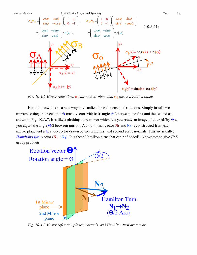
14
σφσ X =cosφ sinφsinφ −cosφ
⎛
⎝⎜⎜
⎞
⎠⎟⎟
1 00 −1
⎛
⎝⎜⎞
⎠⎟ , σ Xσφ = 1 0
0 −1
⎛
⎝⎜⎞
⎠⎟cosφ sinφsinφ −cosφ
⎛
⎝⎜⎜
⎞
⎠⎟⎟
=cosφ −sinφsinφ cosφ
⎛
⎝⎜⎜
⎞
⎠⎟⎟
=R[φ] , =cosφ −sinφsinφ cosφ
⎛
⎝⎜⎜
⎞
⎠⎟⎟
=R[-φ]
(10.A.11)
φ/2
φσφ|x〉=cosφ|x〉+sinφ|y〉
σφ|y〉= sinφ|x〉−cosφ|y〉
|x〉
|y〉|y〉
|x〉
σA|x〉= |x〉
σA|x〉=−|y〉
σφσAσB
Fig. 10.A.6 Mirror reflections σA through xz-plane and σφ through rotated plane.
Hamilton saw this as a neat way to visualize three-dimensional rotations. Simply install two mirrors so they intersect on a Θ crank vector with half-angle Θ/2 between the first and the second as shown in Fig. 10.A.7. It is like a clothing store mirror which lets you rotate an image of yourself by Θ as you adjust the angle Θ/2 between mirrors. A unit normal vector N1 and N2 is constructed from each mirror plane and a Θ/2 arc-vector drawn between the first and second plane normals. This arc is called Hamilton's turn vector (N1→N2). It is these Hamilton turns that can be "added" like vectors to give U(2) group products!
N1
N2Hamilton TurnN1→→N2
Θ/2Rotation vectorΘΘRotation angle = Θ
(Θ/2 Arc)
1st Mirrorplane2nd Mirrorplane
Fig. 10.A.7 Mirror reflection planes, normals, and Hamilton-turn arc vector.
HarterSoft –LearnIt Unit 3 Fourier Analysis and Symmetry 10-A
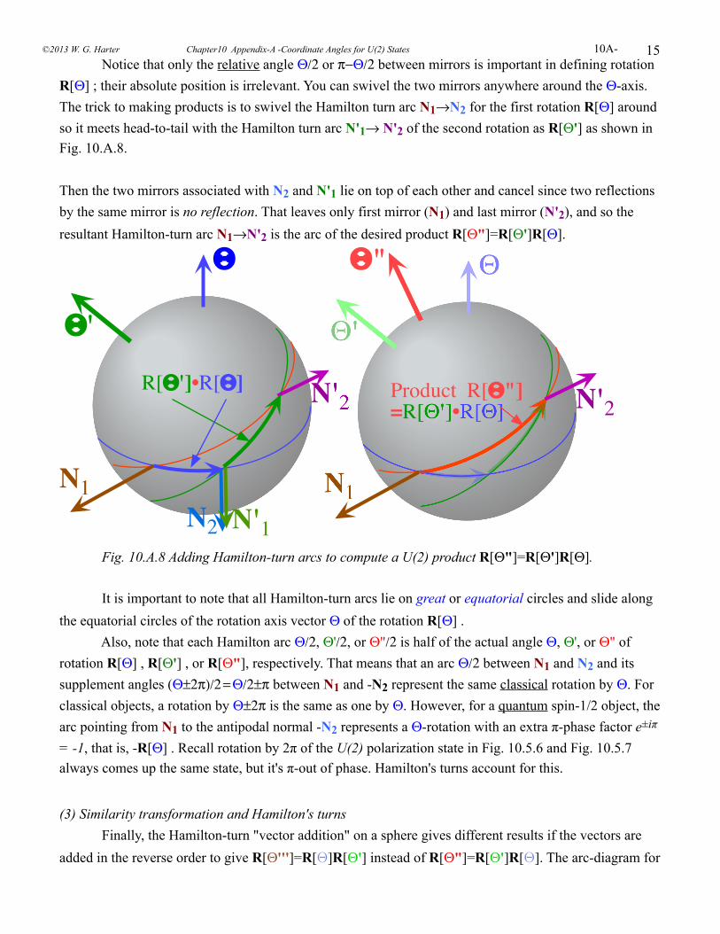
15 Notice that only the relative angle Θ/2 or π−Θ/2 between mirrors is important in defining rotation R[Θ] ; their absolute position is irrelevant. You can swivel the two mirrors anywhere around the Θ-axis. The trick to making products is to swivel the Hamilton turn arc N1→N2 for the first rotation R[Θ] around so it meets head-to-tail with the Hamilton turn arc N'1→ N'2 of the second rotation as R[Θ'] as shown in Fig. 10.A.8.
Then the two mirrors associated with N2 and N'1 lie on top of each other and cancel since two reflections by the same mirror is no reflection. That leaves only first mirror (N1) and last mirror (N'2), and so the resultant Hamilton-turn arc N1→N'2 is the arc of the desired product R[Θ"]=R[Θ']R[Θ].
N1N2 N'1
N'2
ΘΘ
ΘΘ'
R[ΘΘ']•R[ΘΘ]
N1
N'2
ΘΘ"
Product R[ΘΘ"]=R[ΘΘ']•R[ΘΘ]
Fig. 10.A.8 Adding Hamilton-turn arcs to compute a U(2) product R[Θ"]=R[Θ']R[Θ].
It is important to note that all Hamilton-turn arcs lie on great or equatorial circles and slide along the equatorial circles of the rotation axis vector Θ of the rotation R[Θ] . Also, note that each Hamilton arc Θ/2, Θ'/2, or Θ"/2 is half of the actual angle Θ, Θ', or Θ" of rotation R[Θ] , R[Θ'] , or R[Θ"], respectively. That means that an arc Θ/2 between N1 and N2 and its supplement angles (Θ±2π)/2 = Θ/2±π between N1 and -N2 represent the same classical rotation by Θ. For classical objects, a rotation by Θ±2π is the same as one by Θ. However, for a quantum spin-1/2 object, the arc pointing from N1 to the antipodal normal -N2 represents a Θ-rotation with an extra π-phase factor e±iπ = -1, that is, -R[Θ] . Recall rotation by 2π of the U(2) polarization state in Fig. 10.5.6 and Fig. 10.5.7 always comes up the same state, but it's π-out of phase. Hamilton's turns account for this.
(3) Similarity transformation and Hamilton's turns Finally, the Hamilton-turn "vector addition" on a sphere gives different results if the vectors are added in the reverse order to give R[Θ''']=R[Θ]R[Θ'] instead of R[Θ"]=R[Θ']R[Θ]. The arc-diagram for
©2013 W. G. Harter Chapter10 Appendix-A -Coordinate Angles for U(2) States 10A-
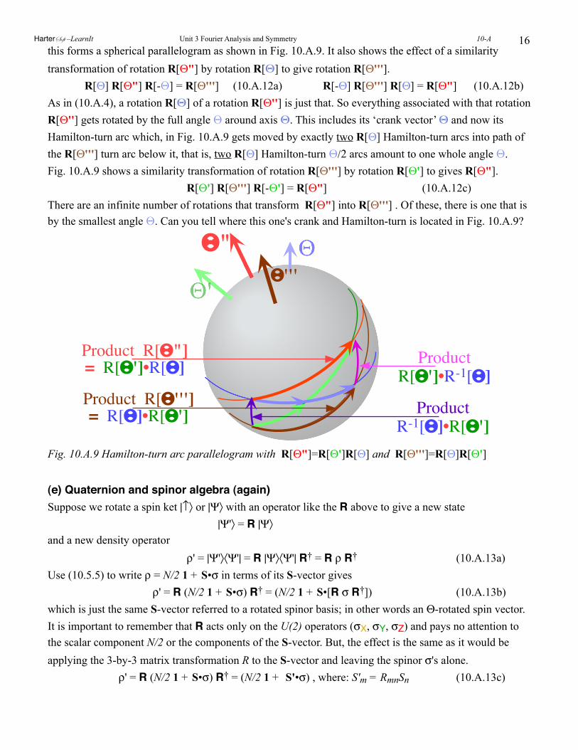
16this forms a spherical parallelogram as shown in Fig. 10.A.9. It also shows the effect of a similarity transformation of rotation R[Θ"] by rotation R[Θ] to give rotation R[Θ''']. R[Θ] R[Θ"] R[-Θ] = R[Θ'''] (10.A.12a) R[-Θ] R[Θ'''] R[Θ] = R[Θ"] (10.A.12b)As in (10.A.4), a rotation R[Θ] of a rotation R[Θ''] is just that. So everything associated with that rotation R[Θ''] gets rotated by the full angle Θ around axis Θ. This includes its ‘crank vector’ Θ and now its Hamilton-turn arc which, in Fig. 10.A.9 gets moved by exactly two R[Θ] Hamilton-turn arcs into path of the R[Θ'''] turn arc below it, that is, two R[Θ] Hamilton-turn Θ/2 arcs amount to one whole angle Θ.Fig. 10.A.9 shows a similarity transformation of rotation R[Θ'''] by rotation R[Θ'] to gives R[Θ"]. R[Θ'] R[Θ'''] R[-Θ'] = R[Θ"] (10.A.12c)There are an infinite number of rotations that transform R[Θ"] into R[Θ'''] . Of these, there is one that is by the smallest angle Θ. Can you tell where this one's crank and Hamilton-turn is located in Fig. 10.A.9?
ΘΘ"
Product R[ΘΘ"]= R[ΘΘ']•R[ΘΘ]
Product R[ΘΘ''']= R[ΘΘ]•R[ΘΘ']
ΘΘ'''
ProductR[ΘΘ']•R-1[ΘΘ]
ProductR-1[ΘΘ]•R[ΘΘ']
Fig. 10.A.9 Hamilton-turn arc parallelogram with R[Θ"]=R[Θ']R[Θ] and R[Θ''']=R[Θ]R[Θ']
(e) Quaternion and spinor algebra (again)Suppose we rotate a spin ket |↑〉 or |Ψ〉 with an operator like the R above to give a new state |Ψ'〉 = R |Ψ〉 and a new density operator ρ' = |Ψ'〉〈Ψ'| = R |Ψ〉〈Ψ'| R† = R ρ R† (10.A.13a)Use (10.5.5) to write ρ = N/2 1 + S•σ in terms of its S-vector gives ρ' = R (N/2 1 + S•σ) R† = (N/2 1 + S•[R σ R†]) (10.A.13b)which is just the same S-vector referred to a rotated spinor basis; in other words an Θ-rotated spin vector. It is important to remember that R acts only on the U(2) operators (σX, σY, σZ) and pays no attention to the scalar component N/2 or the components of the S-vector. But, the effect is the same as it would be applying the 3-by-3 matrix transformation R to the S-vector and leaving the spinor σ's alone. ρ' = R (N/2 1 + S•σ) R† = (N/2 1 + S'•σ) , where: S'm = RmnSn (10.A.13c)
HarterSoft –LearnIt Unit 3 Fourier Analysis and Symmetry 10-A
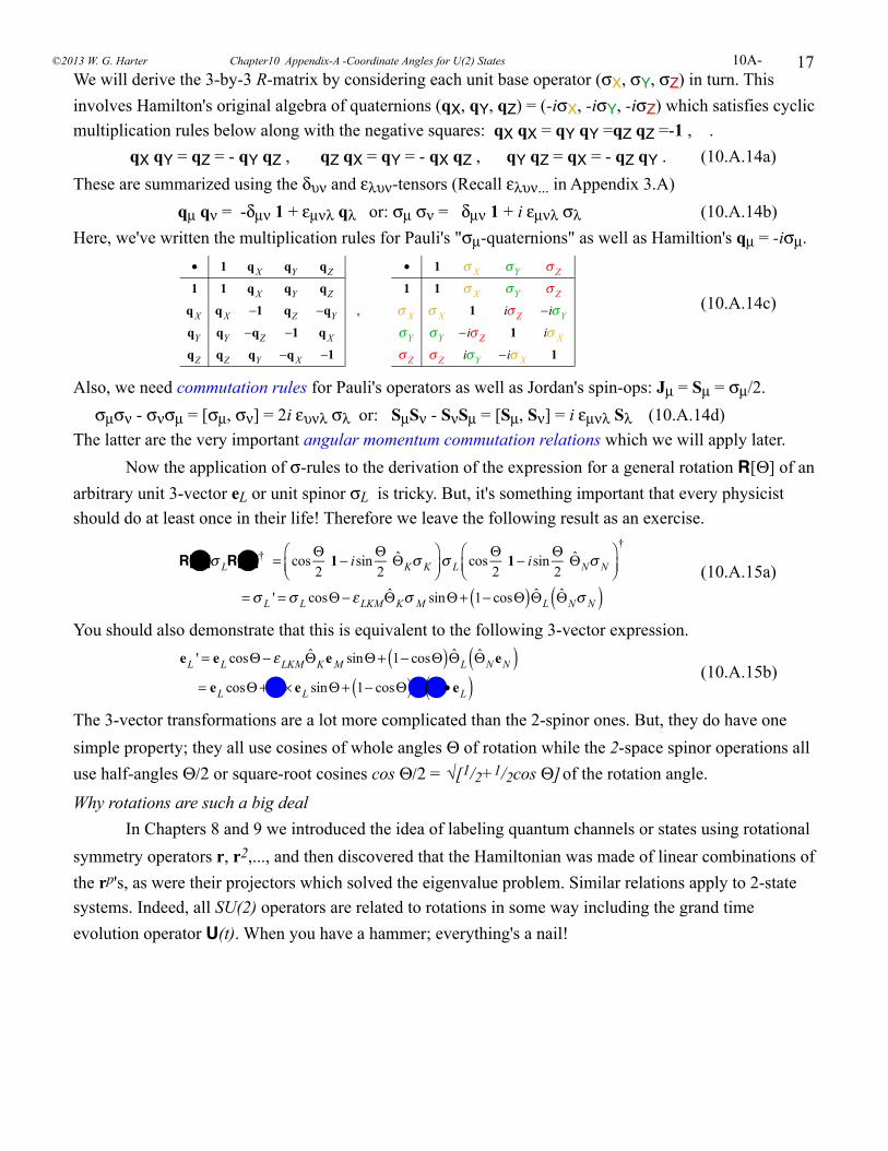
17We will derive the 3-by-3 R-matrix by considering each unit base operator (σX, σY, σZ) in turn. This involves Hamilton's original algebra of quaternions (qX, qY, qZ) = (-iσX, -iσY, -iσZ) which satisfies cyclic multiplication rules below along with the negative squares: qX qX = qY qY =qZ qZ =-1 , . qX qY = qZ = - qY qZ , qZ qX = qY = - qX qZ , qY qZ = qX = - qZ qY . (10.A.14a)These are summarized using the δυν and ελυν-tensors (Recall ελυν... in Appendix 3.A) qµ qν = -δµν 1 + εµνλ qλ or: σµ σν = δµν 1 + i εµνλ σλ (10.A.14b)Here, we've written the multiplication rules for Pauli's "σµ-quaternions" as well as Hamiltion's qµ = -iσµ.
• 1 qX qY qZ
1 1 qX qY qZ
qX qX −1 qZ −qY
qY qY −qZ −1 qX
qZ qZ qY −qX −1
,
• 1 σ X σY σ Z
1 1 σ X σY σ Z
σ X σ X 1 iσ Z −iσY
σY σY −iσ Z 1 iσ X
σ Z σ Z iσY −iσ X 1
(10.A.14c)
Also, we need commutation rules for Pauli's operators as well as Jordan's spin-ops: Jµ = Sµ = σµ/2. σµσν - σνσµ = [σµ, σν] = 2i ευνλ σλ or: SµSν - SνSµ = [Sµ, Sν] = i εµνλ Sλ (10.A.14d)The latter are the very important angular momentum commutation relations which we will apply later. Now the application of σ-rules to the derivation of the expression for a general rotation R[Θ] of an arbitrary unit 3-vector eL or unit spinor σL is tricky. But, it's something important that every physicist should do at least once in their life! Therefore we leave the following result as an exercise.
R[Θ]σ LR[
Θ]† = cos
Θ2
1− isinΘ2
ΘKσ K⎛⎝⎜
⎞⎠⎟σ L cos
Θ2
1− isinΘ2
ΘNσ N⎛⎝⎜
⎞⎠⎟
†
=σ L ' =σ L cosΘ− εLKMΘKσ M sinΘ + 1− cosΘ( )ΘL ΘNσ N( ) (10.A.15a)
You should also demonstrate that this is equivalent to the following 3-vector expression.
eL ' = eL cosΘ− εLKMΘKe M sinΘ + 1− cosΘ( )ΘL ΘN eN( ) = eL cosΘ + Θ × eL sinΘ + 1− cosΘ( )Θ Θ • eL( ) (10.A.15b)
The 3-vector transformations are a lot more complicated than the 2-spinor ones. But, they do have one simple property; they all use cosines of whole angles Θ of rotation while the 2-space spinor operations all use half-angles Θ/2 or square-root cosines cos Θ/2 = √[1/2+1/2cos Θ] of the rotation angle.
Why rotations are such a big deal In Chapters 8 and 9 we introduced the idea of labeling quantum channels or states using rotational symmetry operators r, r2,..., and then discovered that the Hamiltonian was made of linear combinations of the rp's, as were their projectors which solved the eigenvalue problem. Similar relations apply to 2-state systems. Indeed, all SU(2) operators are related to rotations in some way including the grand time evolution operator U(t). When you have a hammer; everything's a nail!
©2013 W. G. Harter Chapter10 Appendix-A -Coordinate Angles for U(2) States 10A-
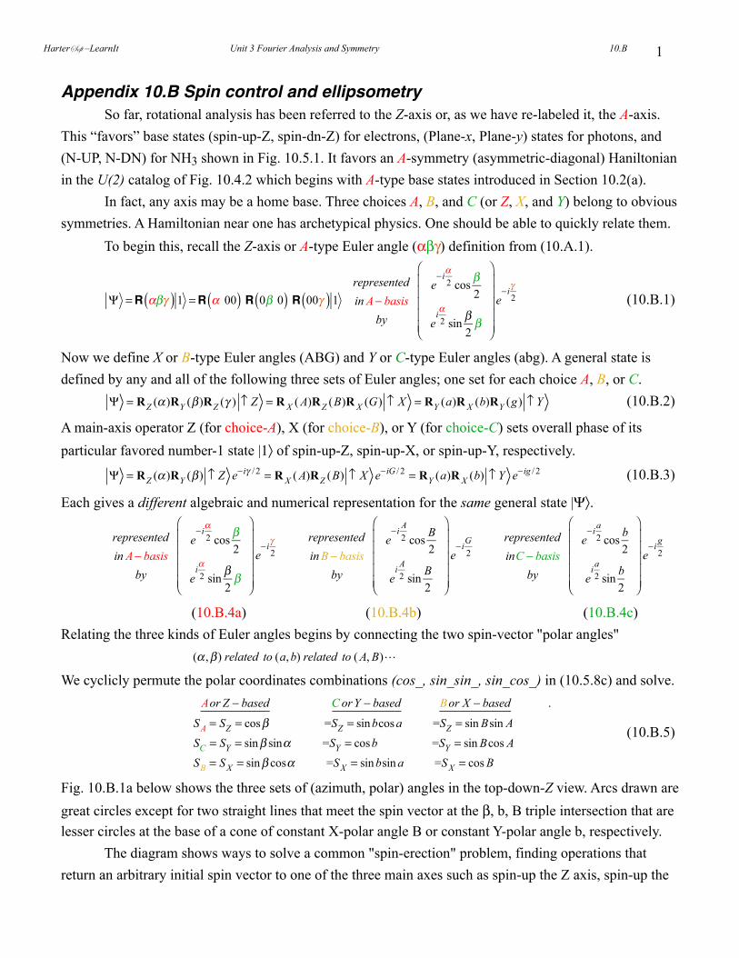
1
Appendix 10.B Spin control and ellipsometry So far, rotational analysis has been referred to the Z-axis or, as we have re-labeled it, the A-axis. This “favors” base states (spin-up-Z, spin-dn-Z) for electrons, (Plane-x, Plane-y) states for photons, and (N-UP, N-DN) for NH3 shown in Fig. 10.5.1. It favors an A-symmetry (asymmetric-diagonal) Haniltonian in the U(2) catalog of Fig. 10.4.2 which begins with A-type base states introduced in Section 10.2(a). In fact, any axis may be a home base. Three choices A, B, and C (or Z, X, and Y) belong to obvious symmetries. A Hamiltonian near one has archetypical physics. One should be able to quickly relate them. To begin this, recall the Z-axis or A-type Euler angle (αβγ) definition from (10.A.1).
Ψ =R αβγ( ) 1 =R α 00( ) R 0β 0( ) R 00γ( ) 1
representedin A− basis
by
e−iα
2 cosβ2
eiα2 sin
β2β
⎛
⎝
⎜⎜⎜⎜⎜
⎞
⎠
⎟⎟⎟⎟⎟
e−iγ
2 (10.B.1)
Now we define X or B-type Euler angles (ABG) and Y or C-type Euler angles (abg). A general state is defined by any and all of the following three sets of Euler angles; one set for each choice A, B, or C.
Ψ = RZ (α )RY (β)RZ (γ ) ↑ Z = R X ( A)RZ (B)R X (G) ↑ X = RY (a)R X (b)RY (g) ↑ Y (10.B.2)
A main-axis operator Z (for choice-A), X (for choice-B), or Y (for choice-C) sets overall phase of its particular favored number-1 state |1〉 of spin-up-Z, spin-up-X, or spin-up-Y, respectively.
: Ψ = RZ (α )RY (β) ↑ Z e−iγ / 2 = R X ( A)RZ (B) ↑ X e−iG / 2 = RY (a)R X (b) ↑ Y e−ig / 2 (10.B.3)
Each gives a different algebraic and numerical representation for the same general state |Ψ〉.
representedin A− basis
by
e−iα
2 cosβ2
eiα2 sin
β2β
⎛
⎝
⎜⎜⎜⎜⎜
⎞
⎠
⎟⎟⎟⎟⎟
e−iγ
2
representedin B − basis
by
e−i A
2 cosB2
ei A2 sin
B2
⎛
⎝
⎜⎜⎜⎜⎜
⎞
⎠
⎟⎟⎟⎟⎟
e−iG
2
representedinC − basis
by
e−i a
2 cosb2
ei a2 sin
b2
⎛
⎝
⎜⎜⎜⎜⎜
⎞
⎠
⎟⎟⎟⎟⎟
e−i g
2
(10.B.4a) (10.B.4b) (10.B.4c)Relating the three kinds of Euler angles begins by connecting the two spin-vector "polar angles" (α ,β) related to (a,b) related to ( A, B)
We cyclicly permute the polar coordinates combinations (cos_, sin_sin_, sin_cos_) in (10.5.8c) and solve.
Aor Z − based C orY − based Bor X − based .
SA = SZ = cosβ =SZ = sinbcosa =SZ = sin Bsin A
SC = SY = sinβ sinα =SY = cosb =SY = sin Bcos A
SB = SX = sinβ cosα =SX = sinbsin a =SX = cos B
(10.B.5)
Fig. 10.B.1a below shows the three sets of (azimuth, polar) angles in the top-down-Z view. Arcs drawn are great circles except for two straight lines that meet the spin vector at the β, b, B triple intersection that are lesser circles at the base of a cone of constant X-polar angle B or constant Y-polar angle b, respectively. The diagram shows ways to solve a common "spin-erection" problem, finding operations that return an arbitrary initial spin vector to one of the three main axes such as spin-up the Z axis, spin-up the
HarterSoft –LearnIt Unit 3 Fourier Analysis and Symmetry 10.B
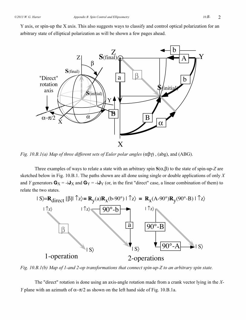
2
Y axis, or spin-up the X axis. This also suggests ways to classify and control optical polarization for an arbitrary state of elliptical polarization as will be shown a few pages ahead.
S(initial)
X
ZS(final) A
B
b
b
B
a
α
β
Yβ
αα−π/2X
"Direct"rotationaxis
Z
YS(initial)
S(final)
Fig. 10.B.1(a) Map of three different sets of Euler polar angles (αβγ) , (abg), and (ABG).
Three examples of ways to relate a state with an arbitrary spin S(α,β) to the state of spin-up-Z are sketched below in Fig. 10.B.1. The paths shown are all done using single or double applications of only X and Y generators GX = -iJX and GY = -iJY (or, in the first "direct" case, a linear combination of them) to relate the two states.
| S〉=Rdirect [β]| ↑z〉 = Ry(a)Rx(b-90°) | ↑z〉 = Rx(A-90°)Ry(90°-B) | ↑z〉
β
90°-b
a 90°-B
90°-A| S〉 | S〉
| ↑z〉 | ↑z〉
| S〉
| ↑z〉
1-operation 2-operationsFig. 10.B.1(b) Map of 1-and 2-op transformations that connect spin-up-Z to an arbitrary spin state.
The "direct" rotation is done using an axis-angle rotation made from a crank vector lying in the X-Y plane with an azimuth of α−π/2 as shown on the left hand side of Fig. 10.B.1a.
©2013 W. G. Harter Appendix B Spin Control and Ellipsometry 10.B-
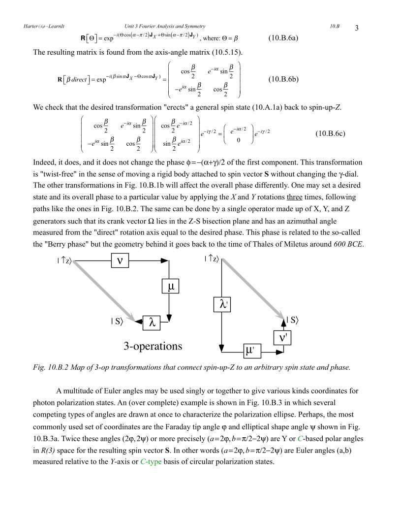
3
R Θ⎡⎣ ⎤⎦ = exp−i(Θcos α−π / 2( )JX +Θ sin α−π / 2( )JY ) , where: Θ = β (10.B.6a)
The resulting matrix is found from the axis-angle matrix (10.5.15).
R β direct⎡⎣ ⎤⎦ = exp−i(β sinαJX −ΘcosαJY ) =cos
β2
e−iα sinβ2
−eiα sinβ2
cosβ2
⎛
⎝
⎜⎜⎜⎜
⎞
⎠
⎟⎟⎟⎟
(10.B.6b)
We check that the desired transformation "erects" a general spin state (10.A.1a) back to spin-up-Z.
cosβ2
e−iα sinβ2
−eiα sinβ2
cosβ2
⎛
⎝
⎜⎜⎜⎜
⎞
⎠
⎟⎟⎟⎟
cosβ2
e−iα / 2
sinβ2
eiα / 2
⎛
⎝
⎜⎜⎜⎜
⎞
⎠
⎟⎟⎟⎟
e−iγ / 2 = e−iα / 2
0
⎛
⎝⎜
⎞
⎠⎟ e−iγ / 2 (10.B.6c)
Indeed, it does, and it does not change the phase φ = −(α+γ)/2 of the first component. This transformation is "twist-free" in the sense of moving a rigid body attached to spin vector S without changing the γ-dial. The other transformations in Fig. 10.B.1b will affect the overall phase differently. One may set a desired state and its overall phase to a particular value by applying the X and Y rotations three times, following paths like the ones in Fig. 10.B.2. The same can be done by a single operator made up of X, Y, and Z generators such that its crank vector Ω lies in the Z-S bisection plane and has an azimuthal angle measured from the "direct" rotation axis equal to the desired phase. This phase is related to the so-called the "Berry phase" but the geometry behind it goes back to the time of Thales of Miletus around 600 BCE.
| S〉 | S〉
| ↑z〉 | ↑z〉
3-operations
µλ'
µ'
λν'
ν
Fig. 10.B.2 Map of 3-op transformations that connect spin-up-Z to an arbitrary spin state and phase.
A multitude of Euler angles may be used singly or together to give various kinds coordinates for photon polarization states. An (over complete) example is shown in Fig. 10.B.3 in which several competing types of angles are drawn at once to characterize the polarization ellipse. Perhaps, the most commonly used set of coordinates are the Faraday tip angle ϕ and elliptical shape angle ψ shown in Fig. 10.B.3a. Twice these angles (2ϕ, 2ψ) or more precisely (a = 2ϕ, b = π/2−2ψ) are Y or C-based polar angles in R(3) space for the resulting spin vector S. In other words (a = 2ϕ, b = π/2−2ψ) are Euler angles (a,b) measured relative to the Y-axis or C-type basis of circular polarization states.
HarterSoft –LearnIt Unit 3 Fourier Analysis and Symmetry 10.B

4
No less useful, however, are a set of coordinates (2ϑ, 2ν) based upon the Z-axis or A-type basis of x and y plane polarization. These are the standard Euler angles (α,β) introduced previously. Not shown in the Fig. 10.B.3 is a third set of angles based upon the bilaterally symmetric B-type basis of ±45° plane polarization states or NH3 eigenstates. All these possible coordinates have varying advantages and disadvantages which depend on what Hamiltonian and physics is being studied.
©2013 W. G. Harter Appendix B Spin Control and Ellipsometry 10.B-
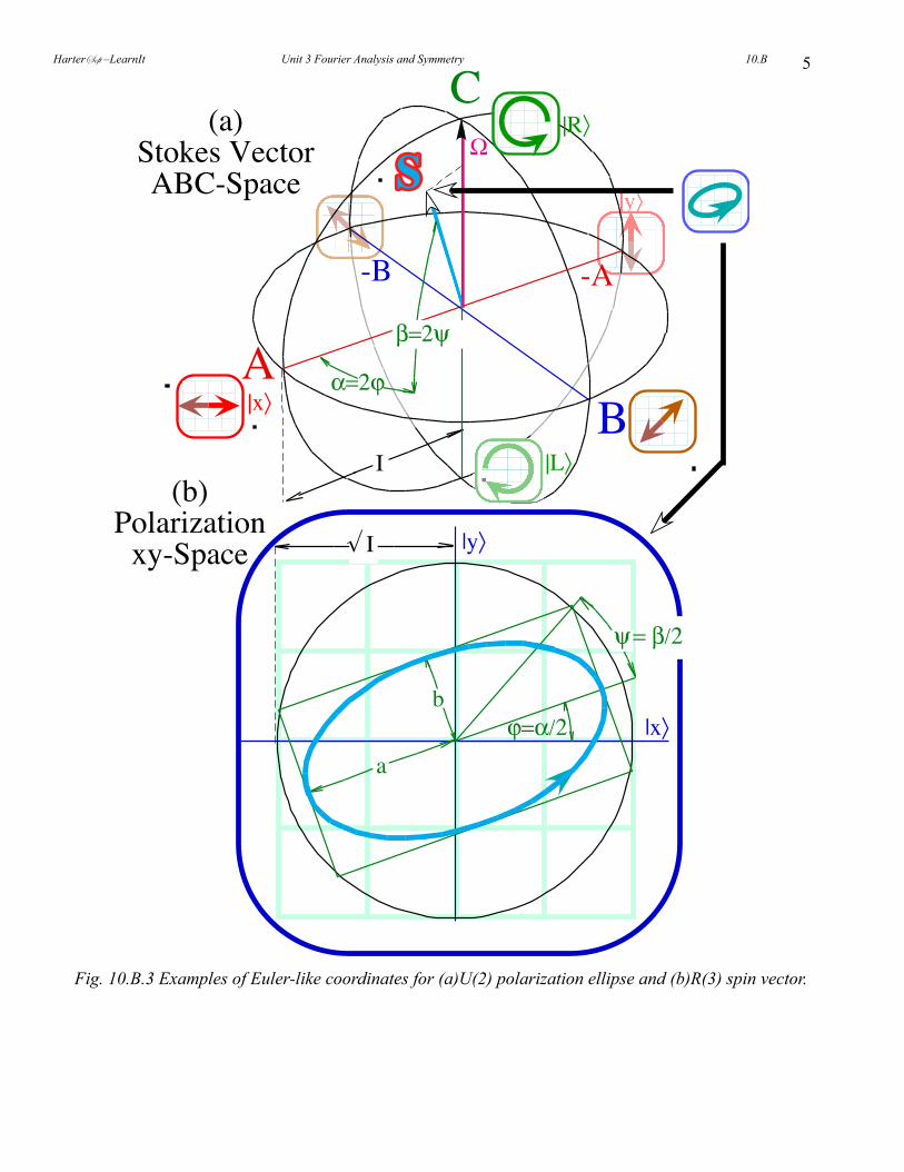
5
|y〉
I
AB
C
SSΩ
α=2ϕ
β=2ψ
(a)Stokes VectorABC-Space
(b)Polarizationxy-Space
|x〉
√ I
ϕ=α/2a
b
|y〉
|R〉
|x〉
|L〉
-A-B
ψ= β/2
Fig. 10.B.3 Examples of Euler-like coordinates for (a)U(2) polarization ellipse and (b)R(3) spin vector.
HarterSoft –LearnIt Unit 3 Fourier Analysis and Symmetry 10.B
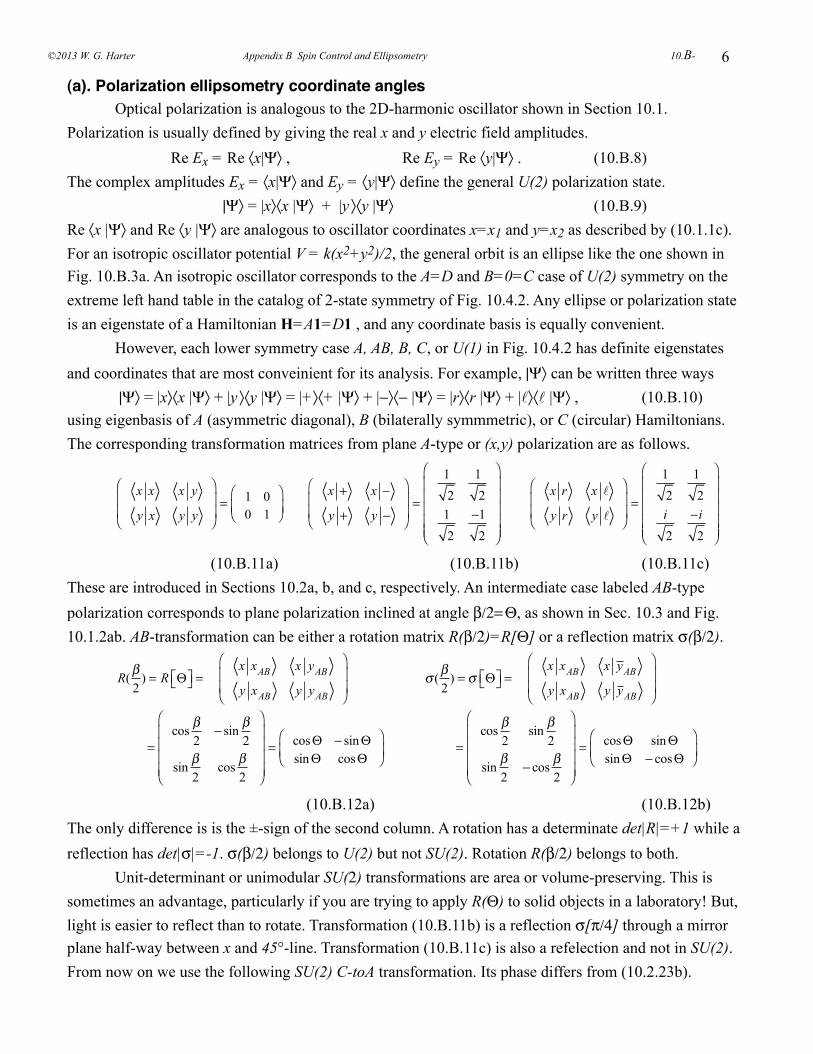
6
(a). Polarization ellipsometry coordinate angles Optical polarization is analogous to the 2D-harmonic oscillator shown in Section 10.1. Polarization is usually defined by giving the real x and y electric field amplitudes. Re Ex = Re 〈x|Ψ〉 , Re Ey = Re 〈y|Ψ〉 . (10.B.8)The complex amplitudes Ex = 〈x|Ψ〉 and Ey = 〈y|Ψ〉 define the general U(2) polarization state. |Ψ〉 = |x〉〈x |Ψ〉 + |y 〉〈y |Ψ〉 (10.B.9)Re 〈x |Ψ〉 and Re 〈y |Ψ〉 are analogous to oscillator coordinates x=x1 and y=x2 as described by (10.1.1c). For an isotropic oscillator potential V = k(x2+y2)/2, the general orbit is an ellipse like the one shown in Fig. 10.B.3a. An isotropic oscillator corresponds to the A=D and B=0=C case of U(2) symmetry on the extreme left hand table in the catalog of 2-state symmetry of Fig. 10.4.2. Any ellipse or polarization state is an eigenstate of a Hamiltonian H=A1=D1 , and any coordinate basis is equally convenient. However, each lower symmetry case A, AB, B, C, or U(1) in Fig. 10.4.2 has definite eigenstates and coordinates that are most conveinient for its analysis. For example, |Ψ〉 can be written three ways |Ψ〉 = |x〉〈x |Ψ〉 + |y 〉〈y |Ψ〉 = |+〉〈+ |Ψ〉 + |−〉〈− |Ψ〉 = |r〉〈r |Ψ〉 + |〉〈 |Ψ〉 , (10.B.10)using eigenbasis of A (asymmetric diagonal), B (bilaterally symmmetric), or C (circular) Hamiltonians. The corresponding transformation matrices from plane A-type or (x,y) polarization are as follows.
x x x y
y x y y
⎛
⎝⎜⎜
⎞
⎠⎟⎟= 1 0
0 1
⎛
⎝⎜⎞
⎠⎟
x + x −
y + y −
⎛
⎝⎜⎜
⎞
⎠⎟⎟=
12
12
12
−12
⎛
⎝
⎜⎜⎜⎜⎜
⎞
⎠
⎟⎟⎟⎟⎟
x r x
y r y
⎛
⎝⎜⎜
⎞
⎠⎟⎟=
12
12
i
2−i
2
⎛
⎝
⎜⎜⎜⎜⎜
⎞
⎠
⎟⎟⎟⎟⎟
(10.B.11a) (10.B.11b) (10.B.11c)These are introduced in Sections 10.2a, b, and c, respectively. An intermediate case labeled AB-type polarization corresponds to plane polarization inclined at angle β/2= Θ, as shown in Sec. 10.3 and Fig. 10.1.2ab. AB-transformation can be either a rotation matrix R(β/2)=R[Θ] or a reflection matrix σ(β/2).
R(β2
) = R Θ⎡⎣ ⎤⎦ = x xAB x yAB
y xAB y yAB
⎛
⎝⎜⎜
⎞
⎠⎟⎟
=cos
β2
− sinβ2
sinβ2
cosβ2
⎛
⎝
⎜⎜⎜⎜
⎞
⎠
⎟⎟⎟⎟
= cosΘ − sinΘsinΘ cosΘ
⎛
⎝⎜⎞
⎠⎟
σ (β2
) = σ Θ⎡⎣ ⎤⎦ = x xAB x yAB
y xAB y yAB
⎛
⎝⎜⎜
⎞
⎠⎟⎟
=cos
β2
sinβ2
sinβ2
− cosβ2
⎛
⎝
⎜⎜⎜⎜
⎞
⎠
⎟⎟⎟⎟
= cosΘ sinΘsinΘ − cosΘ
⎛
⎝⎜⎞
⎠⎟
(10.B.12a) (10.B.12b)The only difference is is the ±-sign of the second column. A rotation has a determinate det|R|=+1 while a reflection has det|σ|=-1. σ(β/2) belongs to U(2) but not SU(2). Rotation R(β/2) belongs to both. Unit-determinant or unimodular SU(2) transformations are area or volume-preserving. This is sometimes an advantage, particularly if you are trying to apply R(Θ) to solid objects in a laboratory! But, light is easier to reflect than to rotate. Transformation (10.B.11b) is a reflection σ[π/4] through a mirror plane half-way between x and 45°-line. Transformation (10.B.11c) is also a refelection and not in SU(2). From now on we use the following SU(2) C-toA transformation. Its phase differs from (10.2.23b).
©2013 W. G. Harter Appendix B Spin Control and Ellipsometry 10.B-
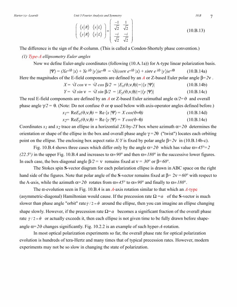
7
x R x L
y R y L
⎛
⎝⎜⎜
⎞
⎠⎟⎟=
−12
12
−i
2−i
2
⎛
⎝
⎜⎜⎜⎜⎜
⎞
⎠
⎟⎟⎟⎟⎟
(10.B.13)
The difference is the sign of the R-column. (This is called a Condon-Shortely phase convention.)
(1) Type-A ellipsometry Euler angles Now we define Euler-angle coordinates (following (10.A.1a)) for A-type linear polarization basis.
|Ψ〉 = (Xe-iϑ |x〉 + Ye iϑ |y 〉)e-iθ = √I(cosν e-iϑ |x〉 + sinν e iϑ |y 〉)e-iθ (10.B.14a)Here the magnitudes of the E-field components are defined by an A or Z-based Euler polar angle β=2ν . X = √I cos ν = √I cos β/2 = |Ex(ϑ,ν,θ)|=|〈x |Ψ〉| (10.B.14b) Y = √I sin ν = √I sin β/2 = |Ey(ϑ,ν,θ)|=|〈y |Ψ〉| (10.B.14c)The real E-field components are defined by an A or Z-based Euler azimuthal angle α/2=ϑ and overall phase angle γ/2 = θ. (Note: Do not confuse ϑ or ϕ used below with axis-operator angles defined before.) x1= ReEx(ϑ,ν,θ) = Re 〈x |Ψ〉 = X cos(ϑ+θ) (10.B.14d) x2= ReEy(ϑ,ν,θ) = Re 〈y |Ψ〉 = Y cos(ϑ−θ) (10.B.14e)Coordinates x1 and x2 trace an ellipse in a horizontial 2X-by-2Y box where azimuth α=2ϑ determines the orientation or shape of the ellipse in the box and overall phase angle γ =2θ ("twist") locates each orbiting point on the ellipse. The enclosing box aspect ratio X:Y is fixed by polar angle β=2ν in (10.B.14b-c). Fig. 10.B.4 shows three cases which differ only by the angle α=2ϑ which has value α= 45°=2(22.5°) in the upper Fig. 10.B.4 and increases to α= 90° and then α= 180° in the successive lower figures. In each case, the box-diagonal angle β/2 = ν remains fixed at ν = 30° or β=60°. The Stokes spin S-vector diagram for each polarization ellipse is drawn in ABC space on the right hand side of the figures. Note that polar angle of the S-vector remains fixed at β= 2ν =60° with respect to the A-axis, while the azimuth α=2ϑ rotates from α= 45° to α= 90° and finally to α= 180°. The α-evolution seen in Fig. 10.B.4 is an A-axis rotation similar to that which an A-type (asymmetric-diagonal) Hamiltonian would cause. If the precession rate Ω = α of the S-vector is much slower than phase angle "orbit" rate γ / 2 = θ around the ellipse, then you can imagine an ellipse changing
shape slowly. However, if the precession rate Ω= α becomes a significant fraction of the overall phase rate γ / 2 = θ or actually exceeds it, then each ellipse is not given time to be fully drawn before shape-
angle α=2ϑ changes significantly. Fig. 10.2.2 is an example of such hyper-A-rotation. In most optical polarization experiments so far, the overall phase rate for optical polarization evolution is hundreds of tera-Hertz and many times that of typical precession rates. However, modern experiments may not be so slow in changing the state of polarization.
HarterSoft –LearnIt Unit 3 Fourier Analysis and Symmetry 10.B
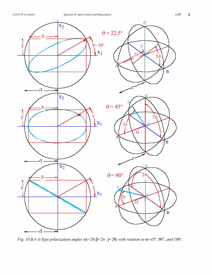
8
X1
X2
√I
ν= 30°
X
Y
I
AB
C
S
2ν 2ϑ
ϑ = 22.5°
X1
X2
√I
ν
X
Y
X1
X2
√I
ν
X
Y
AB
C
S
Ω2ν
2ϑϑ = 90°
I
AB
C S
Ω
2ν
ϑ = 45°
2ϑ
Fig. 10.B.4 A-Type polarization angles (α=2ϑ,β=2ν ,γ=2θ) with rotation to α= 45°, 90°, and 180°.
©2013 W. G. Harter Appendix B Spin Control and Ellipsometry 10.B-
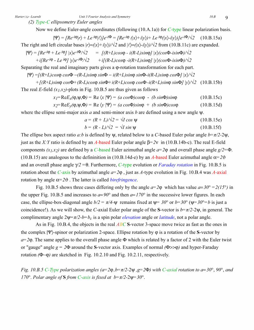
9 (2) Type-C ellipsometry Euler angles Now we define Euler-angle coordinates (following (10.A.1a)) for C-type linear polarization basis.
|Ψ〉 = [Re-iϕ|r〉 + Le iϕ|〉]e-iΦ = [Re-iϕ (|x〉+i|y〉)+ Le iϕ(|x〉-i|y〉)]e-iΦ/√2 (10.B.15a)The right and left circular bases |r〉=(|x〉+i|y〉)/√2 and |〉=(|x〉-i|y〉)/√2 from (10.B.11c) are expanded. |Ψ〉 = [Re-iϕ + Le iϕ] |x〉e-iΦ/√2 = [(R+L)cosϕ - i(R-L)sinϕ] |x〉(cosΦ-isinΦ)/√2 +i[Re-iϕ - Le iϕ] |y〉e-iΦ/√2 +i[(R-L)cosϕ -i(R+L)sinϕ] |y〉(cosΦ-isinΦ)/√2 Separating the real and imaginary parts gives a ϕ-rotation transformation for each part. |Ψ〉 =[(R+L)cosϕ cosΦ −(R-L)sinϕ sinΦ − i(R+L)sinϕ sinΦ-i(R-L)sinϕ cosΦ] |x〉/√2 +[(R+L)sinϕ cosΦ+(R-L)cosϕ sinΦ+i(R+L)cosϕ cosΦ -i(R+L)sinϕ sinΦ] |y〉/√2 (10.B.15b)The real E-field (x1,x2)-plots in Fig. 10.B.5 are thus given as follows x1=ReEx(ϕ,ψ,Φ) = Re 〈x |Ψ〉 = (a cosΦ)cosϕ - (b sinΦ)sinϕ (10.B.15c) x2=ReEy(ϕ,ψ,Φ) = Re 〈y |Ψ〉 = (a cosΦ)sinϕ + (b sinΦ)cosϕ (10.B.15d)where the ellipse semi-major axis a and semi-minor axis b are defined using a new angle ψ. a = (R + L)/√2 = √I cos ψ (10.B.15e) b = (R - L)/√2 = √I sin ψ (10.B.15f)The ellipse box aspect ratio a:b is defined by ψ, related below to a C-based Euler polar angle b=π/2-2ψ, just as the X:Y ratio is defined by an A-based Euler polar angle β=2ν in (10.B.14b-c). The real E-field components (x1,x2) are defined by a C-based Euler azimuthal angle a=2ϕ and overall phase angle g/2=Φ. (10.B.15) are analogous to the defininition in (10.B.14d-e) by an A-based Euler azimuthal angle α=2ϑ and an overall phase angle γ/2 =θ. Furthermore, C-type evolution or Faraday rotation in Fig. 10.B.5 is rotation about the C-axis by azimuthal angle a=2ϕ , just as A-type evolution in Fig. 10.B.4 was A-axial rotation by angle α=2ϑ . The latter is called birefringence. Fig. 10.B.5 shows three cases differing only by the angle a=2ϕ which has value a= 30° =2(15°) in the upper Fig. 10.B.5 and increases to a= 90° and then a= 170° in the successive lower figures. In each case, the ellipse-box-diagonal angle b/2 = π/4-ψ remains fixed at ψ= 30° or b=30° (ψ=30°=b is just a coincidence!). As we will show, the C-axial Euler polar angle of the S-vector is b=π/2-2ψ, in general. The complimentary angle 2ψ=π/2-b=bc is a spin polar elevation angle or latitude, not a polar angle. As in Fig. 10.B.4, the objects in the real ABC S-vector 3-space move twice as fast as the ones in the complex |Ψ〉-spinor or polarization 2-space. Ellipse rotation by ϕ is a rotation of the S-vector by a=2ϕ. The same applies to the overall phase angle Φ which is related by a factor of 2 with the Euler twist or "gauge" angle g = 2Φ around the S-vector axis. Examples of normal (Φ>>ϕ) and hyper-Faraday rotation (Φ∼ϕ) are sketched in Fig. 10.2.10 and Fig. 10.2.11, respectively.
Fig. 10.B.5 C-Type polarization angles (a=2ϕ ,b=π/2-2ψ ,g=2Φ) with C-axial rotation to a= 30°, 90°, and 170°. Polar angle of S from C-axis is fixed at b=π/2-2ψ=30°.
HarterSoft –LearnIt Unit 3 Fourier Analysis and Symmetry 10.B
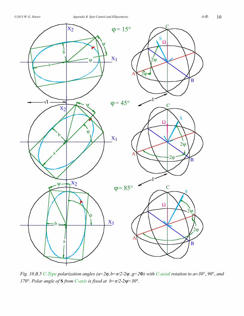
10
X1
X2
ϕ
ψ
a
b
I
AB
C
S Ω
2ϕ
2ψ
ϕ = 45°
X1
X2
√I
ϕ
ψ
a
b
I
AB
C
S
2ϕ
2ψ
Ω
ϕ = 15°
X1
X2
ϕ
ψ
a
b
AB
C S
2ϕ
2ψ Ω
ϕ = 85°
Fig. 10.B.5 C-Type polarization angles (a=2ϕ ,b=π/2-2ψ ,g=2Φ) with C-axial rotation to a= 30°, 90°, and 170°. Polar angle of S from C-axis is fixed at b=π/2-2ψ=30°.
©2013 W. G. Harter Appendix B Spin Control and Ellipsometry 10.B-
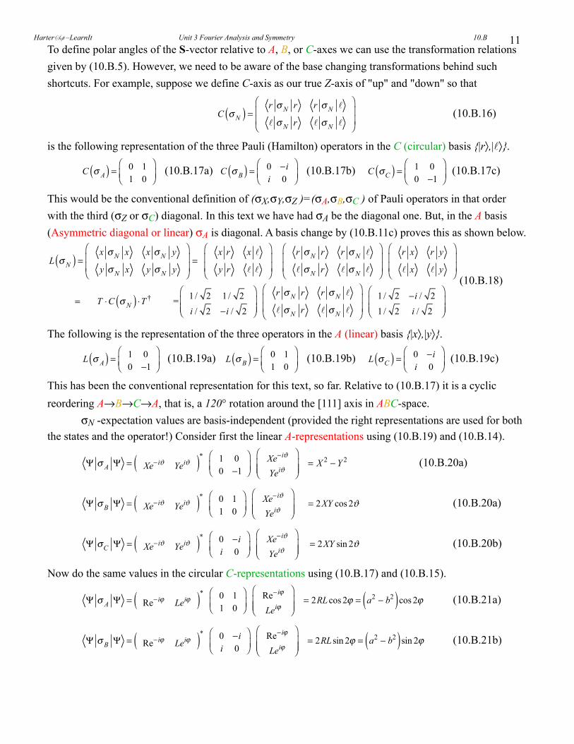
11To define polar angles of the S-vector relative to A, B, or C-axes we can use the transformation relations given by (10.B.5). However, we need to be aware of the base changing transformations behind such shortcuts. For example, suppose we define C-axis as our true Z-axis of "up" and "down" so that
C σN( ) = r σN r r σN
σN r σN
⎛
⎝⎜⎜
⎞
⎠⎟⎟
(10.B.16)
is the following representation of the three Pauli (Hamilton) operators in the C (circular) basis {|r〉,|〉}.
C σ A( ) = 0 1
1 0
⎛
⎝⎜⎞
⎠⎟ (10.B.17a)
C σ B( ) = 0 −i
i 0
⎛
⎝⎜⎞
⎠⎟ (10.B.17b)
C σC( ) = 1 0
0 −1
⎛
⎝⎜⎞
⎠⎟ (10.B.17c)
This would be the conventional definition of (σX,σY,σZ )=(σA,σB,σC ) of Pauli operators in that order with the third (σZ or σC) diagonal. In this text we have had σA be the diagonal one. But, in the A basis (Asymmetric diagonal or linear) σA is diagonal. A basis change by (10.B.11c) proves this as shown below.
L σN( ) = x σN x x σN y
y σN x y σN y
⎛
⎝⎜⎜
⎞
⎠⎟⎟=
x r x
y r
⎛
⎝⎜⎜
⎞
⎠⎟⎟
r σN r r σN
σN r σN
⎛
⎝⎜⎜
⎞
⎠⎟⎟
r x r y
x y
⎛
⎝⎜⎜
⎞
⎠⎟⎟
= T ⋅C σN( ) ⋅T † = 1 / 2 1 / 2i / 2 −i / 2
⎛
⎝⎜⎜
⎞
⎠⎟⎟
r σN r r σN
σN r σN
⎛
⎝⎜⎜
⎞
⎠⎟⎟
1 / 2 −i / 21 / 2 i / 2
⎛
⎝⎜⎜
⎞
⎠⎟⎟
(10.B.18)
The following is the representation of the three operators in the A (linear) basis {|x〉,|y〉}.
L σ A( ) = 1 0
0 −1
⎛
⎝⎜⎞
⎠⎟ (10.B.19a)
L σ B( ) = 0 1
1 0
⎛
⎝⎜⎞
⎠⎟ (10.B.19b)
L σC( ) = 0 −i
i 0
⎛
⎝⎜⎞
⎠⎟ (10.B.19c)
This has been the conventional representation for this text, so far. Relative to (10.B.17) it is a cyclic reordering A→B→C→A, that is, a 120° rotation around the [111] axis in ABC-space. σN -expectation values are basis-independent (provided the right representations are used for both the states and the operator!) Consider first the linear A-representations using (10.B.19) and (10.B.14).
Ψ σ A Ψ = Xe−iϑ Yeiϑ( )* 1 00 −1
⎛
⎝⎜⎞
⎠⎟ Xe−iϑ
Yeiϑ
⎛
⎝⎜⎜
⎞
⎠⎟⎟
= X 2 − Y 2 (10.B.20a)
Ψ σ B Ψ = Xe−iϑ Yeiϑ( )* 0 11 0
⎛
⎝⎜⎞
⎠⎟ Xe−iϑ
Yeiϑ
⎛
⎝⎜⎜
⎞
⎠⎟⎟
= 2XY cos 2ϑ (10.B.20a)
Ψ σC Ψ = Xe−iϑ Yeiϑ( )* 0 −ii 0
⎛
⎝⎜⎞
⎠⎟ Xe−iϑ
Yeiϑ
⎛
⎝⎜⎜
⎞
⎠⎟⎟
= 2XY sin 2ϑ (10.B.20b)
Now do the same values in the circular C-representations using (10.B.17) and (10.B.15).
Ψ σ A Ψ = Re−iϕ Leiϕ( )* 0 11 0
⎛
⎝⎜⎞
⎠⎟ Re−iϕ
Leiϕ
⎛
⎝⎜⎜
⎞
⎠⎟⎟
= 2RLcos 2ϕ = a2 − b2( )cos 2ϕ (10.B.21a)
Ψ σ B Ψ = Re−iϕ Leiϕ( )* 0 −ii 0
⎛
⎝⎜⎞
⎠⎟ Re−iϕ
Leiϕ
⎛
⎝⎜⎜
⎞
⎠⎟⎟
= 2RL sin 2ϕ = a2 − b2( )sin 2ϕ (10.B.21b)
HarterSoft –LearnIt Unit 3 Fourier Analysis and Symmetry 10.B
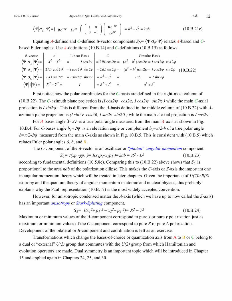
12
Ψ σC Ψ = Re−iϕ Leiϕ( )* 1 00 −1
⎛
⎝⎜⎞
⎠⎟ Re−iϕ
Leiϕ
⎛
⎝⎜⎜
⎞
⎠⎟⎟
= R2 − L2 = 2ab (10.B.21c)
Equating A-defined and C-defined S-vector components SN= 〈Ψ|σN|Ψ〉 relates A-based and C-based Euler angles. Use A-definitions (10.B.14) and C-definitions (10.B.15) as follows.
S-vector A Linear Basis C Circular Basis
Ψ σ A Ψ = X 2 − Y 2 = I cos 2ν = 2RLcos 2ϕ = (a2 − b2 )cos 2ϕ = I cos 2ψ cos 2ϕ
Ψ σ B Ψ = 2XY cos 2ϑ = I cos 2ϑ sin 2ν = 2RL sin 2ϕ = (a2 − b2 ) sin 2ϕ = I cos 2ψ sin 2ϕ
Ψ σC Ψ = 2XY sin 2ϑ = I sin 2ϑ sin 2ν = R2 − L2 = 2ab = I sin 2ψ
Ψ 1 Ψ = X 2 + Y 2 = I = R2 + L2 = a2 + b2
(10.B.22)
First notice how the polar coordinates for the C-basis are defined in the right-most column of (10.B.22). The C-azimuth plane projection is (I cos2ψ cos2ϕ, I cos2ψ sin2ϕ ) while the main C-axial projection is I sin2ψ . This is different from the A-basis defined in the middle column of (10.B.22) with A-azimuth plane projection is (I sin2ν cos2ϑ, I sin2ν sin2ϑ ) while the main A-axial projection is I cos2ν . For A-bases angle β=2ν is a true polar angle measured from the main A-axis as shown in Fig. 10.B.4. For C-bases angle bc=2ψ is an elevation angle or complement bc=π/2-b of a true polar angle b=π/2-2ψ measured from the main C-axis as shown in Fig. 10.B.5. This is consistent with (10.B.5) which relates Euler polar angles β, b, and B. The C-component of the S-vector is an oscillator or "photon" angular momentum component SC= I(xpy-ypx )= I(x1p2-x2p1 )=2ab = R2 - L2 (10.B.23)according to fundamental definitions (10.5.8c). Comparing this to (10.B.22) above shows that SC is proportional to the area πab of the polarization ellipse. This makes the C-axis or Z-axis the important one in angular momentum theory which will be treated in later chapters. Given the importance of U(2)>R(3) isotropy and the quantum theory of angular momentum in atomic and nuclear physics, this probably explains why the Pauli representation (10.B.17) is the most widely accepted convention. However, for anisotropic condensed matter the A-axis (which we have up to now called the Z-axis) has an important anisotropy or Stark-Splitting component. SA= I(x12+ p1 2 − x22− p2 2)= X2 − Y2 (10.B.24)Maximum or minimum values of the A-component correspond to pure x or pure y polarization just as maximum or minimum values of the C-component correspond to pure R or pure L polarization. Development of the bilateral or B-component and coordination is left as an exercise. Transformations which change the bases-of-choice or quantization axis from A to B or C belong to a dual or “external” U(2) group that commutes with the U(2) group from which Hamiltonian and evolution operators are made. Dual symmetry is an important topic which will be introduced in Chapter 15 and applied again in Chapters 24, 25, and 30.
©2013 W. G. Harter Appendix B Spin Control and Ellipsometry 10.B-
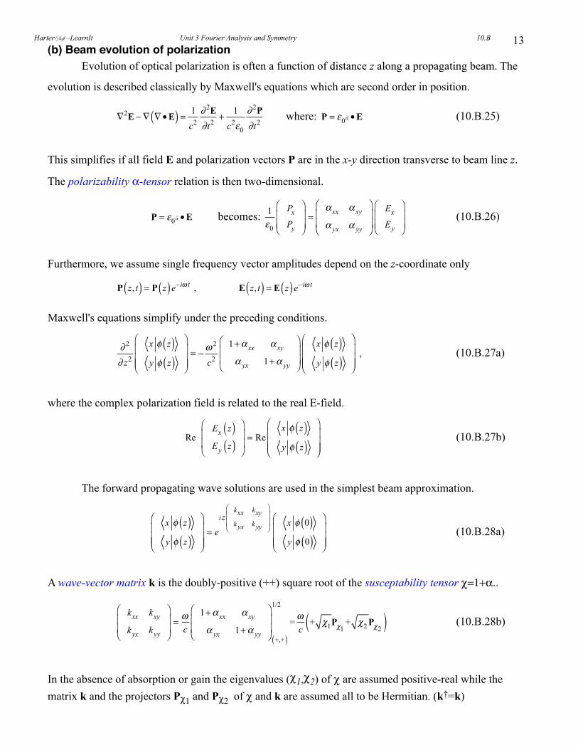
13(b) Beam evolution of polarization Evolution of optical polarization is often a function of distance z along a propagating beam. The
evolution is described classically by Maxwell's equations which are second order in position.
∇2E − ∇ ∇ •E( ) = 1
c2∂2E∂t2
+ 1c2ε0
∂2P∂t2
where: P = ε0α •E (10.B.25)
This simplifies if all field E and polarization vectors P are in the x-y direction transverse to beam line z.
The polarizability α-tensor relation is then two-dimensional.
P = ε0α •E becomes:
1ε0
Px
Py
⎛
⎝⎜⎜
⎞
⎠⎟⎟=
α xx α xy
α yx α yy
⎛
⎝⎜⎜
⎞
⎠⎟⎟
Ex
Ey
⎛
⎝⎜⎜
⎞
⎠⎟⎟
(10.B.26)
Furthermore, we assume single frequency vector amplitudes depend on the z-coordinate only
P z, t( ) = P z( )e−iω t , E z, t( ) = E z( )e−iω t
Maxwell's equations simplify under the preceding conditions.
∂2
∂ z2
x φ z( )y φ z( )
⎛
⎝
⎜⎜⎜
⎞
⎠
⎟⎟⎟= − ω
2
c2
1+α xx α xy
α yx 1+α yy
⎛
⎝⎜⎜
⎞
⎠⎟⎟
x φ z( )y φ z( )
⎛
⎝
⎜⎜⎜
⎞
⎠
⎟⎟⎟
, (10.B.27a)
where the complex polarization field is related to the real E-field.
Re Ex z( )Ey z( )
⎛
⎝
⎜⎜
⎞
⎠
⎟⎟= Re
x φ z( )y φ z( )
⎛
⎝
⎜⎜⎜
⎞
⎠
⎟⎟⎟
(10.B.27b)
The forward propagating wave solutions are used in the simplest beam approximation.
x φ z( )y φ z( )
⎛
⎝
⎜⎜⎜
⎞
⎠
⎟⎟⎟= e
izkxx kxykyx kyy
⎛
⎝
⎜⎜
⎞
⎠
⎟⎟ x φ 0( )
y φ 0( )⎛
⎝
⎜⎜⎜
⎞
⎠
⎟⎟⎟
(10.B.28a)
A wave-vector matrix k is the doubly-positive (++) square root of the susceptability tensor χ=1+α..
kxx kxy
kyx kyy
⎛
⎝⎜⎜
⎞
⎠⎟⎟= ω
c
1+α xx α xy
α yx 1+α yy
⎛
⎝⎜⎜
⎞
⎠⎟⎟
+,+( )
1/2
=ωc
+ χ1Pχ1+ χ2 Pχ2( ) (10.B.28b)
In the absence of absorption or gain the eigenvalues (χ1,χ2) of χ are assumed positive-real while the matrix k and the projectors Pχ1 and Pχ2 of χ and k are assumed all to be Hermitian. (k†=k)
HarterSoft –LearnIt Unit 3 Fourier Analysis and Symmetry 10.B
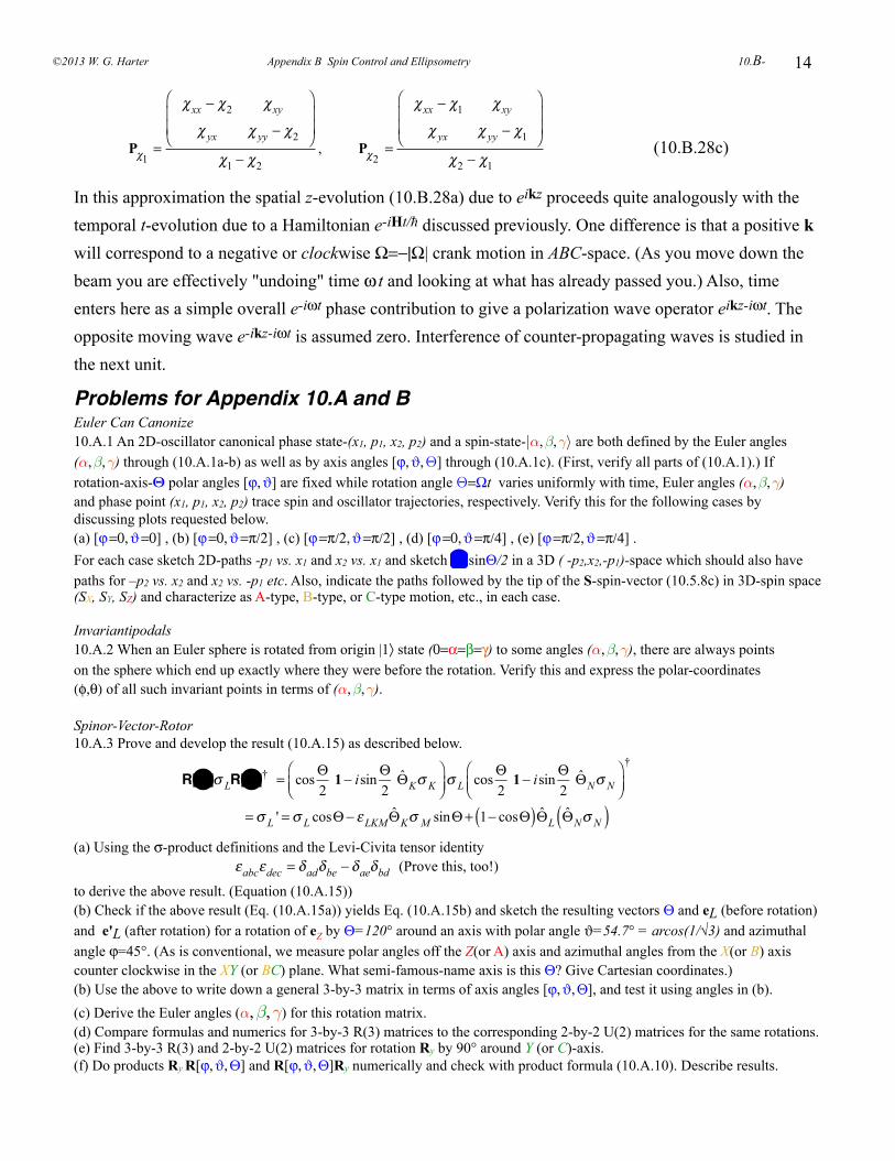
14
Pχ1
=
χxx − χ2 χxy
χ yx χ yy − χ2
⎛
⎝⎜⎜
⎞
⎠⎟⎟
χ1 − χ2, Pχ2
=
χxx − χ1 χxy
χ yx χ yy − χ1
⎛
⎝⎜⎜
⎞
⎠⎟⎟
χ2 − χ1 (10.B.28c)
In this approximation the spatial z-evolution (10.B.28a) due to eikz proceeds quite analogously with the temporal t-evolution due to a Hamiltonian e-iHt/ discussed previously. One difference is that a positive k will correspond to a negative or clockwise Ω=−|Ω| crank motion in ABC-space. (As you move down the beam you are effectively "undoing" time ω t and looking at what has already passed you.) Also, time enters here as a simple overall e-iωt phase contribution to give a polarization wave operator eikz-iωt. The opposite moving wave e-ikz-iωt is assumed zero. Interference of counter-propagating waves is studied in the next unit.
Problems for Appendix 10.A and BEuler Can Canonize10.A.1 An 2D-oscillator canonical phase state-(x1, p1, x2, p2) and a spin-state-⏐α, β, γ〉 are both defined by the Euler angles (α, β, γ) through (10.A.1a-b) as well as by axis angles [ϕ, ϑ, Θ] through (10.A.1c). (First, verify all parts of (10.A.1).) If rotation-axis-Θ polar angles [ϕ, ϑ] are fixed while rotation angle Θ=Ωt varies uniformly with time, Euler angles (α, β, γ) and phase point (x1, p1, x2, p2) trace spin and oscillator trajectories, respectively. Verify this for the following cases by discussing plots requested below. (a) [ϕ =0, ϑ =0] , (b) [ϕ =0, ϑ =π/2] , (c) [ϕ =π/2, ϑ =π/2] , (d) [ϕ =0, ϑ =π/4] , (e) [ϕ =π/2, ϑ =π/4] . For each case sketch 2D-paths -p1 vs. x1 and x2 vs. x1 and sketch Θ sinΘ/2 in a 3D ( -p2,x2,-p1)-space which should also have paths for –p2 vs. x2 and x2 vs. -p1 etc. Also, indicate the paths followed by the tip of the S-spin-vector (10.5.8c) in 3D-spin space(SX, SY, SZ) and characterize as A-type, B-type, or C-type motion, etc., in each case.
Invariantipodals10.A.2 When an Euler sphere is rotated from origin |1〉 state (0=α=β=γ) to some angles (α, β, γ), there are always points on the sphere which end up exactly where they were before the rotation. Verify this and express the polar-coordinates (φ,θ) of all such invariant points in terms of (α, β, γ).
Spinor-Vector-Rotor10.A.3 Prove and develop the result (10.A.15) as described below.
R[Θ]σ LR[
Θ]† = cos
Θ2
1− isinΘ2
ΘKσ K⎛⎝⎜
⎞⎠⎟σ L cos
Θ2
1− isinΘ2
ΘNσ N⎛⎝⎜
⎞⎠⎟
†
=σ L ' =σ L cosΘ− εLKMΘKσ M sinΘ + 1− cosΘ( )ΘL ΘNσ N( )(a) Using the σ-product definitions and the Levi-Civita tensor identity εabcεdec = δadδbe − δaeδbd (Prove this, too!)
to derive the above result. (Equation (10.A.15))(b) Check if the above result (Eq. (10.A.15a)) yields Eq. (10.A.15b) and sketch the resulting vectors Θ and eL (before rotation) and e'L (after rotation) for a rotation of eZ by Θ=120° around an axis with polar angle ϑ=54.7° = arcos(1/√3) and azimuthal angle ϕ=45°. (As is conventional, we measure polar angles off the Z(or A) axis and azimuthal angles from the X(or B) axis counter clockwise in the XY (or BC) plane. What semi-famous-name axis is this Θ? Give Cartesian coordinates.) (b) Use the above to write down a general 3-by-3 matrix in terms of axis angles [ϕ, ϑ, Θ], and test it using angles in (b).(c) Derive the Euler angles (α, β, γ) for this rotation matrix.(d) Compare formulas and numerics for 3-by-3 R(3) matrices to the corresponding 2-by-2 U(2) matrices for the same rotations.(e) Find 3-by-3 R(3) and 2-by-2 U(2) matrices for rotation Ry by 90° around Y (or C)-axis. (f) Do products Ry R[ϕ, ϑ, Θ] and R[ϕ, ϑ, Θ]Ry numerically and check with product formula (10.A.10). Describe results.
©2013 W. G. Harter Appendix B Spin Control and Ellipsometry 10.B-
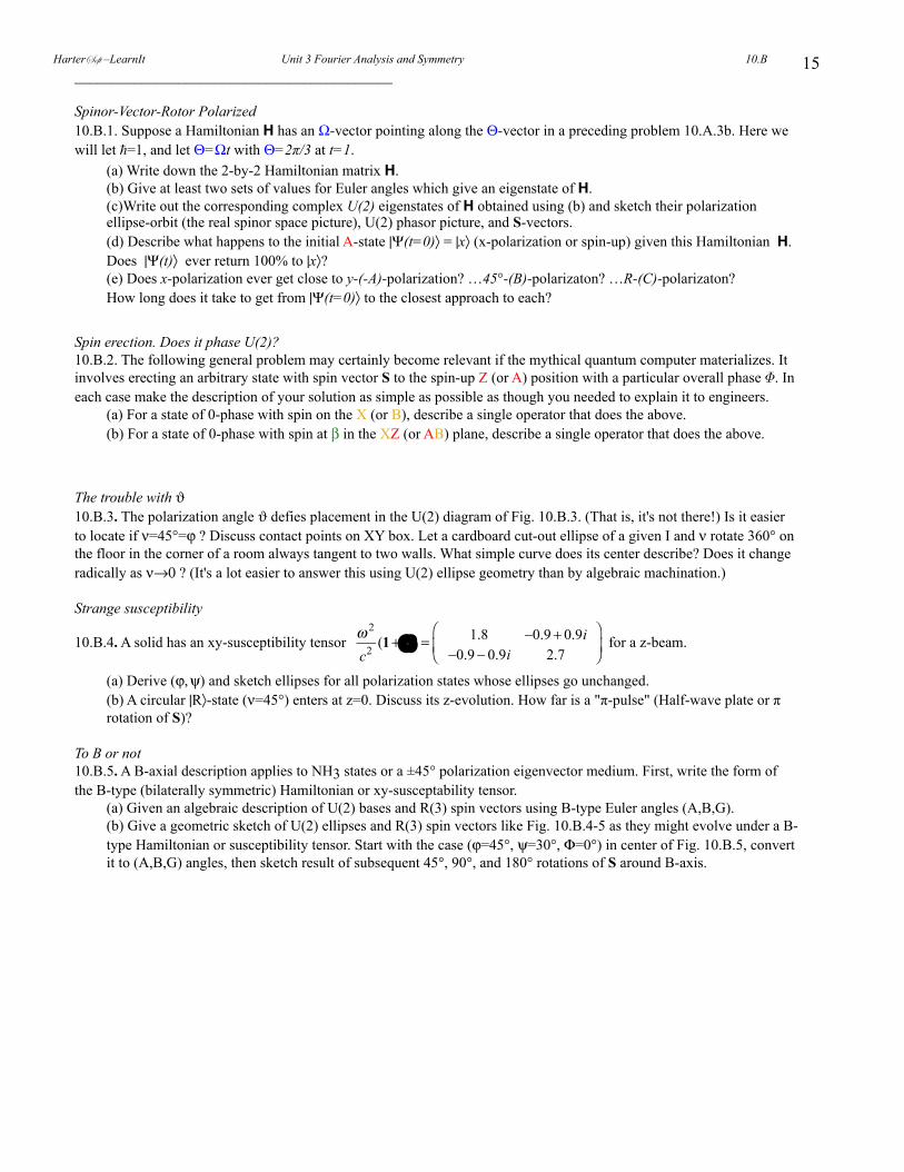
15___________________________________________
Spinor-Vector-Rotor Polarized10.B.1. Suppose a Hamiltonian H has an Ω-vector pointing along the Θ-vector in a preceding problem 10.A.3b. Here we will let =1, and let Θ=Ωt with Θ=2π/3 at t=1.
(a) Write down the 2-by-2 Hamiltonian matrix H.(b) Give at least two sets of values for Euler angles which give an eigenstate of H. (c)Write out the corresponding complex U(2) eigenstates of H obtained using (b) and sketch their polarization ellipse-orbit (the real spinor space picture), U(2) phasor picture, and S-vectors.(d) Describe what happens to the initial A-state |Ψ(t=0)〉 = |x〉 (x-polarization or spin-up) given this Hamiltonian H. Does |Ψ(t)〉 ever return 100% to |x〉? (e) Does x-polarization ever get close to y-(-A)-polarization? …45°-(B)-polarizaton? …R-(C)-polarizaton? How long does it take to get from |Ψ(t=0)〉 to the closest approach to each?
Spin erection. Does it phase U(2)?10.B.2. The following general problem may certainly become relevant if the mythical quantum computer materializes. It involves erecting an arbitrary state with spin vector S to the spin-up Z (or A) position with a particular overall phase Φ. In each case make the description of your solution as simple as possible as though you needed to explain it to engineers.
(a) For a state of 0-phase with spin on the X (or B), describe a single operator that does the above.(b) For a state of 0-phase with spin at β in the XZ (or AB) plane, describe a single operator that does the above.
The trouble with ϑ 10.B.3. The polarization angle ϑ defies placement in the U(2) diagram of Fig. 10.B.3. (That is, it's not there!) Is it easier to locate if ν=45°=ϕ ? Discuss contact points on XY box. Let a cardboard cut-out ellipse of a given I and ν rotate 360° on the floor in the corner of a room always tangent to two walls. What simple curve does its center describe? Does it change radically as ν→0 ? (It's a lot easier to answer this using U(2) ellipse geometry than by algebraic machination.)
Strange susceptibility
10.B.4. A solid has an xy-susceptibility tensor
ω 2
c2 (1+α) = 1.8 −0.9+ 0.9i
−0.9− 0.9i 2.7
⎛
⎝⎜⎞
⎠⎟ for a z-beam.
(a) Derive (ϕ, ψ) and sketch ellipses for all polarization states whose ellipses go unchanged.(b) A circular |R〉-state (ν=45°) enters at z=0. Discuss its z-evolution. How far is a "π-pulse" (Half-wave plate or π rotation of S)?
To B or not 10.B.5. A B-axial description applies to NH3 states or a ±45° polarization eigenvector medium. First, write the form of the B-type (bilaterally symmetric) Hamiltonian or xy-susceptability tensor.
(a) Given an algebraic description of U(2) bases and R(3) spin vectors using B-type Euler angles (A,B,G).(b) Give a geometric sketch of U(2) ellipses and R(3) spin vectors like Fig. 10.B.4-5 as they might evolve under a B-type Hamiltonian or susceptibility tensor. Start with the case (ϕ=45°, ψ=30°, Φ=0°) in center of Fig. 10.B.5, convert it to (A,B,G) angles, then sketch result of subsequent 45°, 90°, and 180° rotations of S around B-axis.
HarterSoft –LearnIt Unit 3 Fourier Analysis and Symmetry 10.B
Related Documents