Quantum Optics for the Impatient Morgan W. Mitchell ICFO - Institut de Ci` encies Fot` oniques Castelldefels Copyright c 2007-2010 Morgan W. Mitchell

Welcome message from author
This document is posted to help you gain knowledge. Please leave a comment to let me know what you think about it! Share it to your friends and learn new things together.
Transcript
Quantum Optics for the Impatient
Morgan W. MitchellICFO - Institut de Ciencies Fotoniques
Castelldefels
Copyright c© 2007-2010 Morgan W. Mitchell

ii
Contents
1 Introduction 1
1.1 What is quantum optics? . . . . . . . . . . . . . . . . . . . . . . . . . . . . 1
1.2 Why do we need quantum optics? . . . . . . . . . . . . . . . . . . . . . . . 1
2 Foundations 3
2.1 Simple harmonic oscillator . . . . . . . . . . . . . . . . . . . . . . . . . . . . 3
2.2 Quantization of the electromagnetic field . . . . . . . . . . . . . . . . . . . . 5
2.2.1 Classical equations of motion . . . . . . . . . . . . . . . . . . . . . . 5
2.3 Quadratures . . . . . . . . . . . . . . . . . . . . . . . . . . . . . . . . . . . . 7
2.4 Connection to classical theory . . . . . . . . . . . . . . . . . . . . . . . . . . 9
3 Quantum states of light 11
3.1 Photons . . . . . . . . . . . . . . . . . . . . . . . . . . . . . . . . . . . . . . 11
3.2 Vacuum . . . . . . . . . . . . . . . . . . . . . . . . . . . . . . . . . . . . . . 11
3.3 Number states . . . . . . . . . . . . . . . . . . . . . . . . . . . . . . . . . . 11
3.4 Coherent states . . . . . . . . . . . . . . . . . . . . . . . . . . . . . . . . . . 12
3.5 Entangled states . . . . . . . . . . . . . . . . . . . . . . . . . . . . . . . . . 16
4 Detection of light 19
4.1 Direct detection and photon counting . . . . . . . . . . . . . . . . . . . . . 19
4.2 Homodyne detection . . . . . . . . . . . . . . . . . . . . . . . . . . . . . . . 22
iii
iv CONTENTS
5 Correlation functions 27
5.1 Quantum correlation functions . . . . . . . . . . . . . . . . . . . . . . . . . 28
5.2 Intensity correlations . . . . . . . . . . . . . . . . . . . . . . . . . . . . . . . 29
5.3 Measuring correlation functions . . . . . . . . . . . . . . . . . . . . . . . . . 30
6 Representations of quantum states of light 33
6.1 Introduction . . . . . . . . . . . . . . . . . . . . . . . . . . . . . . . . . . . . 33
6.2 Density operator . . . . . . . . . . . . . . . . . . . . . . . . . . . . . . . . . 33
6.3 Representation by number states . . . . . . . . . . . . . . . . . . . . . . . . 34
6.4 Representation in terms of quadrature states . . . . . . . . . . . . . . . . . 34
6.5 Representations in terms of coherent states . . . . . . . . . . . . . . . . . . 35
6.5.1 Glauber-Sudarshan P-representation . . . . . . . . . . . . . . . . . . 35
6.5.2 Husimi distribution or Q-representation . . . . . . . . . . . . . . . . 36
6.6 Wigner-Weyl distribution . . . . . . . . . . . . . . . . . . . . . . . . . . . . 36
6.6.1 Classical phase-space distributions . . . . . . . . . . . . . . . . . . . 37
6.6.2 Applying classical statistics to a quantum system . . . . . . . . . . . 37
6.6.3 Facts about the Wigner distribution . . . . . . . . . . . . . . . . . . 39
6.6.4 “Characteristic functions” for Q- and P-distributions . . . . . . . . . 40
7 Proofs of non-classicality 41
7.1 Quantum vs. Classical (vs. Non-classical) . . . . . . . . . . . . . . . . . . . 41
7.2 g(2)(0) . . . . . . . . . . . . . . . . . . . . . . . . . . . . . . . . . . . . . . . 42
7.2.1 Anti-bunching and the P-distribution . . . . . . . . . . . . . . . . . 43
7.3 g(2)(0) variant and the Cauchy-Schwarz inequality. . . . . . . . . . . . . . . 44
7.4 Cauchy-Schwarz inequality . . . . . . . . . . . . . . . . . . . . . . . . . . . . 45
7.5 Bell inequalities . . . . . . . . . . . . . . . . . . . . . . . . . . . . . . . . . . 46
7.6 Squeezing . . . . . . . . . . . . . . . . . . . . . . . . . . . . . . . . . . . . . 46
7.6.1 Classical noise in the fields . . . . . . . . . . . . . . . . . . . . . . . 47
CONTENTS v
7.6.2 Classical square-law detector . . . . . . . . . . . . . . . . . . . . . . 47
7.6.3 Semi-classical square-law detector . . . . . . . . . . . . . . . . . . . 47
7.6.4 Fully quantum detection . . . . . . . . . . . . . . . . . . . . . . . . . 48
7.6.5 Anti-bunching and the P-distribution . . . . . . . . . . . . . . . . . 49
8 Behaviour of quantum fields in linear optics 51
8.1 Diffraction . . . . . . . . . . . . . . . . . . . . . . . . . . . . . . . . . . . . . 51
8.2 Paraxial wave equation . . . . . . . . . . . . . . . . . . . . . . . . . . . . . . 53
8.3 Linear optical elements . . . . . . . . . . . . . . . . . . . . . . . . . . . . . . 53
8.3.1 beam-splitter . . . . . . . . . . . . . . . . . . . . . . . . . . . . . . . 54
8.4 Loss and Gain . . . . . . . . . . . . . . . . . . . . . . . . . . . . . . . . . . . 56
8.4.1 linear amplifiers and attenuators . . . . . . . . . . . . . . . . . . . . 57
8.4.2 phase-insensitive case . . . . . . . . . . . . . . . . . . . . . . . . . . 57
8.4.3 phase-sensitive amplifiers . . . . . . . . . . . . . . . . . . . . . . . . 59
9 Quantum fields in nonlinear optics 61
9.1 Linear and nonlinear optics . . . . . . . . . . . . . . . . . . . . . . . . . . . 61
9.2 Phenomenological approach . . . . . . . . . . . . . . . . . . . . . . . . . . . 62
9.2.1 aside . . . . . . . . . . . . . . . . . . . . . . . . . . . . . . . . . . . . 64
9.2.2 Phenomenological Hamiltonian . . . . . . . . . . . . . . . . . . . . . 65
9.3 Wave-equations approach . . . . . . . . . . . . . . . . . . . . . . . . . . . . 66
9.4 Parametric down-conversion . . . . . . . . . . . . . . . . . . . . . . . . . . . 68
10 Quantum optics with atomic ensembles 71
10.1 Atoms . . . . . . . . . . . . . . . . . . . . . . . . . . . . . . . . . . . . . . . 71
10.1.1 Rotating-wave approximation . . . . . . . . . . . . . . . . . . . . . . 72
10.1.2 First-order light-atom interactions . . . . . . . . . . . . . . . . . . . 72
10.1.3 Second-order light-atom interactions . . . . . . . . . . . . . . . . . . 73
10.2 Atomic ensembles . . . . . . . . . . . . . . . . . . . . . . . . . . . . . . . . . 73
vi CONTENTS
10.2.1 collective excitations . . . . . . . . . . . . . . . . . . . . . . . . . . . 73
10.2.2 collective continuous variables . . . . . . . . . . . . . . . . . . . . . . 76
A Quantum theory for quantum optics 79
A.1 States vs. Operators . . . . . . . . . . . . . . . . . . . . . . . . . . . . . . . 79
A.2 Calculating with operators . . . . . . . . . . . . . . . . . . . . . . . . . . . . 80
A.2.1 Heisenberg equation of motion . . . . . . . . . . . . . . . . . . . . . 80
A.2.2 Time-dependent perturbation theory . . . . . . . . . . . . . . . . . . 80
A.2.3 example: excitation of atoms to second order . . . . . . . . . . . . . 82
A.2.4 Glauber’s broadband detector . . . . . . . . . . . . . . . . . . . . . . 83
A.3 Second quantization . . . . . . . . . . . . . . . . . . . . . . . . . . . . . . . 84
Preface
This text began as notes for the course “Experimental Quantum Optics and QuantumInformation,” attended by students from ICFO and the Barcelona-area universities UAB,UB, and UPC. When the course began, several comprehensive and high-quality books hadrecently been published on quantum optics. These books present, in a complete and coherentfashion, results from decades of work in quantum optics before quantum information becameimportant. They might be compared to Max Born and Emil Wolf’s “Principles of Optics,”which describes the state of knowledge in optics before the invention of the laser. Thesebooks should not be overlooked. Any serious student of quantum optics must be familiarwith at least one authoritative text.
Then why write a new text on Quantum Optics?
Recent progress in quantum optics (QO) has largely been related to quantum information(QI): communications and information processing based on the unique features of quantummechanics. The experimental techniques of quantum optics, which include the precisegeneration, manipulation, and measurement of quantum states of light, are very well suitedto experiments in quantum information. Many problems in quantum information werefirst solved optically. The theory of quantum optics, however, can seem pretty foreignto a practitioner of QI, because QO comes from quantum field theory while QI is fromordinary quantum mechanics. Thus, many students (and others new to the field) arrivewith an interest to understand quantum optics, not for itself, but as a tool for doing (orunderstanding) experimental quantum information. Typically these people are in a hurry.Thus the need for a rapid introduction, a “quick-start” manual, for the area of quantumoptics.
These notes aim to provide a self-contained introduction to quantum optics, for a readershipthat is comfortable with quantum mechanics, electromagnetism, modern optics, and theassociated mathematics. The text presents the core elements of quantum optics theory, theones most likely to be encountered in experimental work or in related theory, in a mannerthat aims to build physical intuition, and will be useful for simple calculations. The textdoes not aim to be comprehensive. Rather, we hope the reader will look to the standardtexts for extensive discussions, historical references, and authoritative formulations. Wehope these texts will be both more interesting and more accessible after this introduction.
vii
viii CONTENTS
Recommended Background
Many fields have contributed to the development of quantum optics, and some prior un-derstanding of these fields is necessary to fully appreciate what happens in quantum opticsexperiments. Most important are physical optics, nonlinear optics, quantum mechanics, andsome basic notions from quantum field theory. Also important are signal theory, atomicphysics, electronics, detector physics, laser theory. The reader is strongly recommended toconsult the books listed below when background information is needed.
Physical Optics and Optical Technologies
Fundamentals of Photonics by B. E. A. Saleh and M. C. Teich, Wiley, 1991.
Nonlinear Optics
Nonlinear Optics, 2nd Ed. by R. W. Boyd, Academic Press, 2002.
Atomic Physics
Laser Spectroscopy: Basic Concepts and Instrumentation by W. Demtroder, Springer, 2000.
Atomic Physics by C. J. Foot, Oxford, 2005.
Laser Physics
Quantum Electronics, 3rd Ed by A. Yariv, Wiley, 1989.
Lasers by A. E. Siegman, University Science Books, 1986.
Laser Physics, New Ed. by M. Sargent, M. O. Scully, W. E. Lamb, Perseus, 1974.
Lasers, 4th Ed. by O. Svelto, Springer, 2004.
Lasers, by P. W. Milonni and J. H. Eberly, Wiley, 1988.
Advanced Mechanics
Classical Mechanics, 3rd Ed. by H. Goldstein, C. P. Poole and J. L. Safko Addison-Wesley,2002.
CONTENTS ix
Electrodynamics
Classical Electrodynamics, 3rd Ed. by J. D. Jackson, Wiley, 1998.
Quantum Mechanics
Modern Quantum Mechanics by J. J. Sakurai, Addison-Wesley, 1985.
Advanced Quantum Mechanics by J. J. Sakurai, Addison-Wesley, 1967.
The Quantum Vacuum: An Introduction to Quantum Electrodynamics by P. W. Milonni,Academic Press, 1993.
Quantum Optics Textbooks
The books listed below are interesting either because they are historical and authoritative,or because they are recent and up-to-date. Almost all cover quantum optics in more detailthan this text. The reader is strongly encouraged to follow at least one of these books atthe same time as reading this text. Much of what is contained in these notes is intended toillustrate or explain what is contained, in denser form, in the books.
Quantum Optics by M. O. Scully and M. S. Zubairy , Cambridge, 1997.
Quantum Optics by D. F. Walls and G. J. Milburn, Springer, 1995.
A Guide to Experiments in Quantum Optics, 2nd Ed. by H-A. Bachor and T. C. Ralph,Wiley, 2004.
The Quantum Theory of Light, 3rd Ed. by R. Loudon, Oxford, 2000.
Optical Coherence and Quantum Optics by L. Mandel and E. Wolf, Cambridge, 1995.
Elements of Quantum Optics, 3rd Ed. by P. Meystre, M. Sargent, Springer, 2006.
Quantum Optics in Phase Space by W. P. Schleich, Wiley, 2001.
Quantum Optics, An Introduction by M. Fox, Oxford, 2006.
Introductory Quantum Optics by C. Gerry, and P. L. Knight Cambridge, 2004.
Methods in Theoretical Quantum Optics by S. M. Barnett and P. M. Radmore, Oxford,2003.
Quantum Optics by W. Vogel and D-G Welsch, Wiley, 2006.
Fundamentals of Quantum Optics and Quantum Information by P. Lambropoulos, D. Pet-rosyan, Springer, 2006.

x CONTENTS
Chapter 1
Introduction
1.1 What is quantum optics?
Quantum optics is the study of light as a quantum system. We all have experience withmaterial quantum systems such as atoms, molecules, or solids. These can often be treatedusing ordinary quantum mechanics: the Schrodinger equation, wave-functions, etc. Light isnot described by ordinary quantum mechanics, but by quantum field theory. This alreadypresents us with a challenge, because quantum field theory was developed to deal withparticle physics, not laser physics. Starting with the work of Roy Glauber in the 1960sand continuing through the present day, theoretical quantum optics has been developedto adapt quantum field theory to the situations encountered in optics: large numbers ofphotons with (sometimes) a high degree of coherence among them, a variety of very precisedetection techniques, and recently the highly non-classical behaviour of entanglement amongphotons or among field modes. Indeed, theoretical quantum optics has been so successfulthat some concepts developed to describe light fields are now applied to other areas, forexample there is currently much interest in the area of “spin squeezing,” even though spinsare not described by a quantum field.
1.2 Why do we need quantum optics?
A classical theory of light is adequate in very many situations. Nevertheless, starting inthe beginning of the 20th century, problems with the classical theory started to emerge.These classic experiments and observations led to the invention of quantum field theoryand quantum optics.
To avoid the “ultraviolet catastrophe,” Planck hypothesized that in a cavity, the energyin any given mode should take on values of E = nhν, where n = 0, 1, 2, . . .. This doesn’trequire that light come in “quanta” with energy hν, but it is suggestive.
1
2 CHAPTER 1. INTRODUCTION
In the photoelectric effect, electrons are ejected from a metal surface by light which fallson the surface. The energy of the electrons thus ejected depends on the frequency of theilluminating light, but not its intensity. This would be easily explained if the energy of aphoton is hν.
In the process of Compton scattering, an x-ray enters a block of material, is deflected, andin the process shifts to longer wavelengths (lower frequency). The shift that was seen waswell explained by considering the x-rays to be composed of photons with energy E = hνand momentum p = hν/c.
Other evidence includes the existence of the Lamb shift, the Casimir effect, and modernexperiments on “non-classical light,” such as squeezed light. Lately, we are interestedin making quantum light do useful things. This includes understanding the fundamentalorigins of noise in measurements and finding ways to reduce noise. Also, there is greatinterest in producing quantum states of light that allow quantum protocols for transmitting,storing, and encrypting information. Quantum computation using quantum states of lightis also an area of active interest.
Chapter 2
Foundations
We begin with the quantization of the electromagnetic field. “Quantization” in this contextmeans inventing a quantum theory which reproduces the results of classical electromag-netism in the classical limit. I say “inventing” rather than “deriving” because in fact thereis no deterministic way to turn a classical theory into a correct quantum theory. Neverthe-less, we will see that the choice is natural, and there is little question that we have the righttheory.
The procedure that we use is called “canonical quantization,” and proceeds from the equa-tions of motion for light (Maxwell’s equations), to a Lagrangian, to an operator representa-tion of the fields. Before we quantize the electromagnetic field, we first quantize somethingsimpler, the harmonic oscillator. In fact, we will see that the electromagnetic field is acollection of harmonic oscillators, so the results will be useful immediately.
2.1 Simple harmonic oscillator
The classical simple harmonic oscillator obeys the following second-order ordinary differen-tial equation
x = −ω2x (2.1)
where x is the position and ω is the angular frequency of oscillation. This equation can bederived from the Lagrangian
L =m
2x2 − mω2
2x2 (2.2)
by applying the Euler-Lagrange equation
d
dt
∂L
∂x=
∂L
∂x(2.3)
Here m is a constant which turns out to be the mass.
3
4 CHAPTER 2. FOUNDATIONS
The canonical momentum conjugate to x is
px ≡ ∂L
∂x= mx. (2.4)
The Hamiltonian is
H ≡∑
i
piqi − L =p2
2m+
mω2
2x2. (2.5)
Note that in this quantization procedure, the equations of motion are fundamental, not theLagrangian or Hamiltonian. Classical theories such as Newton’s laws, Maxwell’s equations,or fluid dynamics, are based in equations of motion. The Lagrangian and Hamiltonian aresecondary, chosen to give the equations of motion.
To create the quantum theory of the harmonic oscillator, we keep this Hamiltonian operatorand we identify x and px as observables and associate them with the operators x and px.In this way the classical Hamiltonian becomes the Hamiltonian operator
H =mω2
2x2 +
12m
p2x. (2.6)
Finally, we assume that these operators have the commutation relation [x, px] = ih. Thisimplies an uncertainty relation δxδpx ≥ h/2. This is the heart of the canonical quantiza-tion procedure: we assume that canonically conjugate coordinates and momenta have thecommutation relation [q, pq] = ih, which replaces the classical relationship involving thePoisson bracket {q, pq}PB = 1.
We note that we can calculate the equations of motion for x and p two ways (and get thesame result). Classically, the Hamilton-Jacobi equations of motion
q =∂H
∂p, p = −∂H
∂q(2.7)
give
x =1m
p
p = −mω2x (2.8)
Quantum mechanically, the Heisenberg equation of motion
A =1ih
[A,H] (2.9)
(valid for any operator A that does not explicitly depend on time) gives
x =1
2imh[x, p2] =
1m
p
p =mω2
2ih[p, x2] = −mω2x. (2.10)
2.2. QUANTIZATION OF THE ELECTROMAGNETIC FIELD 5
More generally, if we have a multi-dimensional system with several coordinates qi and theirconjugate momenta pqi , then we assume the commutation relations [qi, qj ] = [pqi , pqj ] = 0and [qi, pqj ] = ihδij where δij is the Kronecker delta. This implies there is an uncertaintyrelationship only between canonically conjugate variables.
2.2 Quantization of the electromagnetic field
2.2.1 Classical equations of motion
We start with a description of light in empty space, either vacuum or the (empty) inside ofan optical resonator defined by reflecting surfaces such as mirrors. The equations of motionare the source-free Maxwell equations
∇ ·E = 0 (2.11)∇ ·B = 0 (2.12)
∇×E = −∂B∂t
(2.13)
∇×B = µ0ε0∂E∂t
(2.14)
These are simpler in terms of the vector potential A (taken in the Coulomb gauge ∇·A = 0)which satisfies
B = ∇×A
E = −∂A∂t
(2.15)
Substituting into 2.14, we find the wave equation for A(∇2 − 1
c2
∂2
∂t2
)A = 0 (2.16)
It is convenient at this point to expand the spatial part of the vector potential in vectorspatial modes uk,α defined by
∇2uk,α(r) = −k2uk,α(r) (2.17)
where k is the wave-number and α = 1, 2 is an index for the polarization. If we choose thesemodes well, they will be orthonormal,
∫d3r u∗k,α(r) · uk′,α′(r) = δk,k′δα,α′ . Thus the vector
potential isA(r, t) =
∑
k,α
qk,α(t)uk,α(r) (2.18)
where the qk,α are time-varying mode amplitudes. Substituting into equation (2.16), wefind
qk,α = −c2k2qk,α ≡ −ω2kqk,α (2.19)
6 CHAPTER 2. FOUNDATIONS
which is precisely the same form as equation (2.1). Because the equations of motion arethe same, we use the same Lagrangian, and arrive at the same canonical momentum andHamiltonian. The momentum is pk,α = mqk,α. The single-mode Hamiltonian is
Hk,α =12mω2q2
k,α +1
2mp2
k,α. (2.20)
The “mass” m in this equation needs a little explanation. It is not present in the equationsof motion, so it is not determined by the classical dynamics. It is in fact a parameter weare free to choose. As we will see, the right choice for the “mass” is m = ε0, where ε0 is thepermittivity of free space. We also note that the electric field is
E(r, t) = − ∂
∂tA(r, t) = −
∑
k,α
qk,α(t)uk,α(r) = − 1ε0
∑
k,α
pk,α(t)uk,α(r). (2.21)
Thus for each mode uk,α, the vector potential amplitude xA ≡ qk,α is canonically conjugateto −ε0xE where xE ≡ pk,α/ε0 is the electric field amplitude. We now quantize the theoryby replacing the c-numbers qk,α, pk,α with operators qk,α, pk,α which obey the commutationrelation [qk,α, pk,α] = ih. This immediately implies an uncertainty relation for each modeof the A and E fields δxAδxE ≥ h/2ε0.
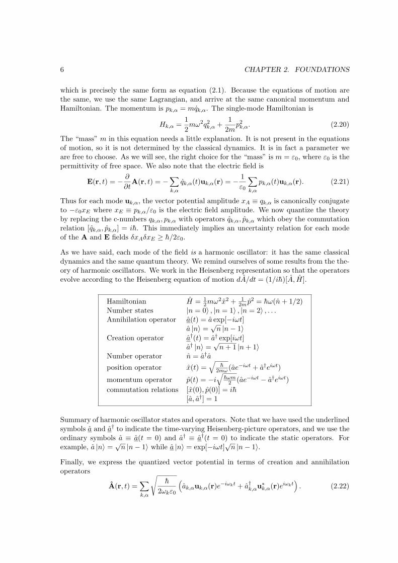
As we have said, each mode of the field is a harmonic oscillator: it has the same classicaldynamics and the same quantum theory. We remind ourselves of some results from the the-ory of harmonic oscillators. We work in the Heisenberg representation so that the operatorsevolve according to the Heisenberg equation of motion dA/dt = (1/ih)[A, H].
Hamiltonian H = 12mω2x2 + 1
2m p2 = hω(n + 1/2)Number states |n = 0〉 , |n = 1〉 , |n = 2〉 , . . .Annihilation operator a(t) = a exp[−iωt]
a |n〉 =√
n |n− 1〉Creation operator a†(t) = a† exp[iωt]
a† |n〉 =√
n + 1 |n + 1〉Number operator n = a†aposition operator x(t) =
√h
2mω (ae−iωt + a†eiωt)
momentum operator p(t) = −i√
hωm2 (ae−iωt − a†eiωt)
commutation relations [x(0), p(0)] = ih[a, a†] = 1
Summary of harmonic oscillator states and operators. Note that we have used the underlinedsymbols a and a† to indicate the time-varying Heisenberg-picture operators, and we use theordinary symbols a ≡ a(t = 0) and a† ≡ a†(t = 0) to indicate the static operators. Forexample, a |n〉 =
√n |n− 1〉 while a |n〉 = exp[−iωt]
√n |n− 1〉.
Finally, we express the quantized vector potential in terms of creation and annihilationoperators
A(r, t) =∑
k,α
√h
2ωkε0
(ak,αuk,α(r)e−iωkt + a†k,αu∗k,α(r)eiωkt
). (2.22)
2.3. QUADRATURES 7
The quantized electric field E = −∂A/∂t is
E(r, t) = i∑
k,α
√hωk
2ε0
(ak,αuk,α(r)e−iωkt − a†k,αu∗k,α(r)eiωkt
)(2.23)
In the case that we are dealing with fields in free space (no resonator to define the modes u),it is conventional to define a “box” of volume L3 to define the modes uk,α(r) = eα exp[ik ·r]/√
L3 where eα are polarization vectors perpendicular to k. In this case the fields are
A(r, t) =∑
k,α
√h
2ωkε0L3
(eαak,αeik·re−iωkt + e∗αa†k,αe−ik·reiωkt
)(2.24)
and
E(r, t) = i∑
k,α
√hωk
2ε0L3
(eαak,αeik·re−iωkt − e∗αa†k,αe−ik·reiωkt
)(2.25)
The quantized magnetic field B = ∇× A is then
B(r, t) = i∑
k,α
√µ0hωk
2L3
(fαak,αeik·re−iωkt − f∗αa†k,αe−ik·reiωkt
)(2.26)
where fα = eα×k/|k| is the magnetic field polarization vector. Using equations (2.25) and(2.26) it is straightforward to verify that the total Hamiltonian describing each mode as aharmonic oscillator,
H =∑
k,α
Hk,α =∑
k,α
12mω2q2
k,α +1
2mp2
k,α =∑
k,α
hωk(a†k,αak,α +
12) (2.27)
agrees with the usual electro-magnetic Hamiltonian
HEM =12
∫d3r
(ε0|E|2 +
1µ0|B|2
)=
∑
k,α
hωk(a†k,αak,α +
12). (2.28)
In fact, this agreement is achieved because we choose m = ε0, as mentioned above.
2.3 Quadratures
Although the vector potential is more fundamental (at least for quantum field theory),in optics we almost always work with the electric field. This is because most materialsinteract more strongly with the electric field than with the magnetic field, and because thevector potential is not very “physical” (it is not gauge invariant, for example). We wouldlike to forget about the vector potential, but somehow keep the quantum physics that issummarized in the uncertainty relationship δxAδxE ≥ h/2ε0. Can we describe everything
8 CHAPTER 2. FOUNDATIONS
we need in terms of just the field E? In fact we can: For a harmonic oscillator, the positionand momentum are always one quarter cycle out of phase. Because of this, if we describethe amplitude of the electric field now, and also a quarter cycle later, we effectively describeboth E and A. Classically, we would write the electric field in terms of two quadratureamplitudes X1, X2 as E(r, t) = X1 sin(ωt − k · r) −X2 cos(ωt − k · r). Here, we define twoquadrature operators X1, X2 through1
E(r, t) =
√hωk
2ε0L3
[X1 sin(ωt− k · r)− X2 cos(ωt− k · r)
]. (2.29)
For this to agree with a single mode’s contribution to equation (2.25)
E(r, t) = i
√hωk
2ε0L3
(ak,αeik·re−iωkt − a†k,αe−ik·reiωkt
)(2.30)
we must have
X1 = a + a† (2.31)X2 = i(a† − a). (2.32)
The quadrature operators are hermitian, and thus observable. In fact, X1 is proportional tothe vector potential amplitude xA at one instant in time and X2 is proportional to electricfield amplitude xE at the same instant in time. They have the commutation relation
[X1, X2] = 2i (2.33)
and uncertainty relationδX1δX2 ≥ 1. (2.34)
Lastly, the Hamiltonian is
H = hω(a†a +12) =
hω
4(X2
1 + X22 ). (2.35)
At just one point in space (or in fact anywhere along a phase front) k · r is a constant.Without loss of generality we choose a point where k · r = 0. At this point the electric fieldis
E(0, t) ∝ X1 sin(ωt) + X2 cos(ωt). (2.36)
This would be the field experienced by a stationary atom, for example. The quadraturesX1 and X2 are simply two coefficients in the Fourier decomposition of the field E(0, t).
1From here on, we are just considering one mode, so we leave out the mode indices k, α and the polariza-tion. We are also explicitly considering a traveling wave, because that is the most familiar situation. A verysimilar derivation can be made assuming standing waves proportional to X1u(r) sin(ωt)−X2u(r) cos(ωt).
2.4. CONNECTION TO CLASSICAL THEORY 9
2.4 Connection to classical theory
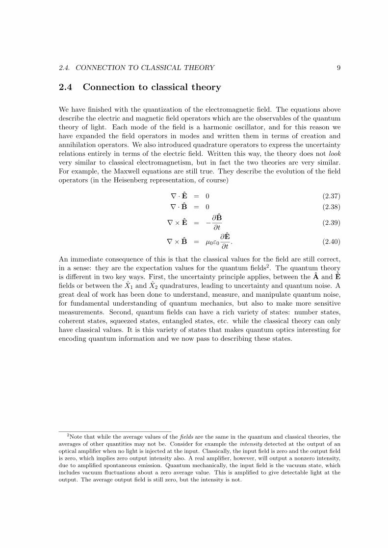
We have finished with the quantization of the electromagnetic field. The equations abovedescribe the electric and magnetic field operators which are the observables of the quantumtheory of light. Each mode of the field is a harmonic oscillator, and for this reason wehave expanded the field operators in modes and written them in terms of creation andannihilation operators. We also introduced quadrature operators to express the uncertaintyrelations entirely in terms of the electric field. Written this way, the theory does not lookvery similar to classical electromagnetism, but in fact the two theories are very similar.For example, the Maxwell equations are still true. They describe the evolution of the fieldoperators (in the Heisenberg representation, of course)
∇ · E = 0 (2.37)∇ · B = 0 (2.38)
∇× E = −∂B∂t
(2.39)
∇× B = µ0ε0∂E∂t
. (2.40)
An immediate consequence of this is that the classical values for the field are still correct,in a sense: they are the expectation values for the quantum fields2. The quantum theoryis different in two key ways. First, the uncertainty principle applies, between the A and Efields or between the X1 and X2 quadratures, leading to uncertainty and quantum noise. Agreat deal of work has been done to understand, measure, and manipulate quantum noise,for fundamental understanding of quantum mechanics, but also to make more sensitivemeasurements. Second, quantum fields can have a rich variety of states: number states,coherent states, squeezed states, entangled states, etc. while the classical theory can onlyhave classical values. It is this variety of states that makes quantum optics interesting forencoding quantum information and we now pass to describing these states.
2Note that while the average values of the fields are the same in the quantum and classical theories, theaverages of other quantities may not be. Consider for example the intensity detected at the output of anoptical amplifier when no light is injected at the input. Classically, the input field is zero and the output fieldis zero, which implies zero output intensity also. A real amplifier, however, will output a nonzero intensity,due to amplified spontaneous emission. Quantum mechanically, the input field is the vacuum state, whichincludes vacuum fluctuations about a zero average value. This is amplified to give detectable light at theoutput. The average output field is still zero, but the intensity is not.

10 CHAPTER 2. FOUNDATIONS
Chapter 3
Quantum states of light
3.1 Photons
The Hamitonian is H = hω(a†a + 1/2). Based on Planck’s hypothesis we believe that aphoton has energy hω, so we interpret the n = a†a as the number of photons in the mode.This means that a(0) destroys a photon, and a†(0) creates one. This is why they’re calledcreation and annihilation operators, after all.
3.2 Vacuum
The ground state of the field is the “vacuum state” |0〉 defined by 〈0| a†a |0〉 = 0. It hasnon-zero energy Evac = hω/2 and fluctuations (∆X1,2)2 =< X2
1,2 > − < X1,2 >2= 1. Thusit is a minimum uncertainty state δX1δX2 = 1.
3.3 Number states
The number states, or “Fock states” are defined by
|n〉 ≡ (a†)n
√n!
|0〉 (3.1)
or n |n〉 = n |n〉. These are energy eigenstates with energy hω(n + 1/2). The number statesare complete and orthonormal, and for many problems, especially those involving photoncounting, they are the most natural basis to use. They are, however, very far from classicalbehaviour. For example, the expectation values of the quadratures are 〈n| X1,2 |n〉 = 0,while the variances are (∆X1,2)2 =< X2
1,2 > − < X1,2 >2= 2n + 1. Viewed in terms ofquadratures, number states consist entirely of noise.
11
12 CHAPTER 3. QUANTUM STATES OF LIGHT
3.4 Coherent states
The energy eigenstates (number states) have zero average field. Clearly this isn’t the casewhen we turn on a laser or a microwave oven. Is there a quantum state that behaves likean oscillating electric field? As in ordinary quantum mechanics, in order for an observableto oscillate, there has to be a superposition of at least two states with different energies. Inthe case of the electric field (or the quadratures) this means there has to be a superpositionof different numbers of photons. What about a state like
|ψ〉 =1√2(|0〉+ |1〉), (3.2)
does this have an oscillating average field? It is easy to show that 〈ψ| X1 |ψ〉 = 1 and〈ψ| X2 |ψ〉 = 0 so that
〈ψ| E(t) |ψ〉 ∝ sin(ωt). (3.3)
So yes, a superposition of energy eigenstates does oscillate. In fact, any field state thatlooks at all classical (that has a nonzero expectation value for the E field) must have anindeterminate number of photons.1
So what sort of field does a laser (or a radio station for that matter) actually produce? Wethink that the classical description of the E-M field should be pretty much correct in thesecases because there are so many photons involved. We want to find a quantum state thatis as classical as possible.
The “most nearly classical” states should have minimum uncertainty δX1δX2 = 1 andshould oscillate like the classical field. It turns out that these states are eigenstates of theannihilation operator a |α〉 = α |α〉. The name “coherent states” was given to this group ofstates by Roy Glauber, who first wrote about them in connection with quantum optics.
A coherent state |α〉 can be expressed in the number basis as
|α〉 = e−|α|2/2
∞∑
n=0
αn
√n!|n〉 . (3.4)
Coherent states have some nice properties.
〈α| X1 |α〉 = 2Re[α] (3.5)〈α| X2 |α〉 = 2Im[α] (3.6)〈α| n |α〉 = |α|2 (3.7)
| 〈n|α〉 |2 =|α|2n
n!e−|α|
2(3.8)
1This is especially strange when you realize that most particles are not allowed to have an indeterminatenumber (at least you can’t get away with hypothesizing the zero/one state above). For example, conservationof lepton number means that while you can lose an electron from the universe, you’re guaranteed to createor destroy at least one other particle (of the electron or neutrino sort) in the process. Your state could be(|0e− > |1νe > +|1e− > |0νe >)/
√2, but that’s not the same thing.
3.4. COHERENT STATES 13
t
t
t
E
E
E
coherent state
squeezed X < 12D
squeezed X < 1D 1
X1
X2
X1
X2
X1
X2
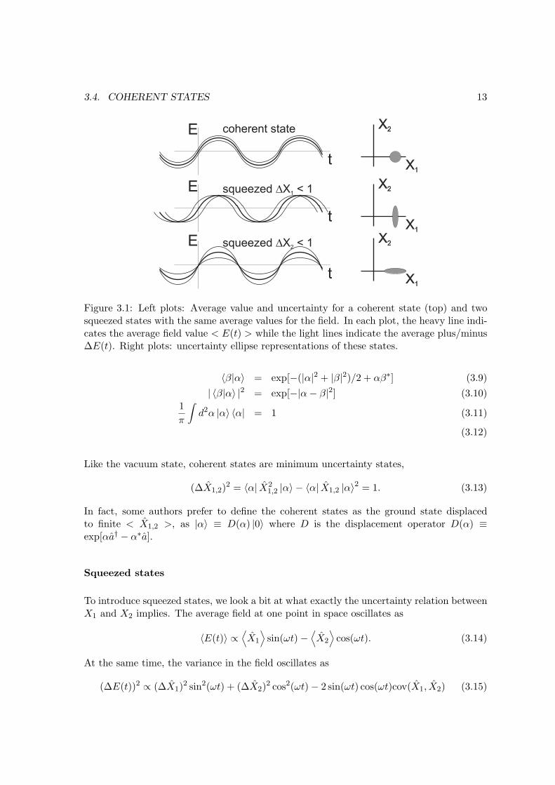
Figure 3.1: Left plots: Average value and uncertainty for a coherent state (top) and twosqueezed states with the same average values for the field. In each plot, the heavy line indi-cates the average field value < E(t) > while the light lines indicate the average plus/minus∆E(t). Right plots: uncertainty ellipse representations of these states.
〈β|α〉 = exp[−(|α|2 + |β|2)/2 + αβ∗] (3.9)| 〈β|α〉 |2 = exp[−|α− β|2] (3.10)
1π
∫d2α |α〉 〈α| = 1 (3.11)
(3.12)
Like the vacuum state, coherent states are minimum uncertainty states,
(∆X1,2)2 = 〈α| X21,2 |α〉 − 〈α| X1,2 |α〉2 = 1. (3.13)
In fact, some authors prefer to define the coherent states as the ground state displacedto finite < X1,2 >, as |α〉 ≡ D(α) |0〉 where D is the displacement operator D(α) ≡exp[αa† − α∗a].
Squeezed states
To introduce squeezed states, we look a bit at what exactly the uncertainty relation betweenX1 and X2 implies. The average field at one point in space oscillates as
〈E(t)〉 ∝⟨X1
⟩sin(ωt)−
⟨X2
⟩cos(ωt). (3.14)
At the same time, the variance in the field oscillates as
(∆E(t))2 ∝ (∆X1)2 sin2(ωt) + (∆X2)2 cos2(ωt)− 2 sin(ωt) cos(ωt)cov(X1, X2) (3.15)
14 CHAPTER 3. QUANTUM STATES OF LIGHT
t
t
t
E
E
E
vacuum state
squeezed vac. X < 1D 1
squeezed vac. X < 1D 2
X1
X2
X1
X2
X1
X2
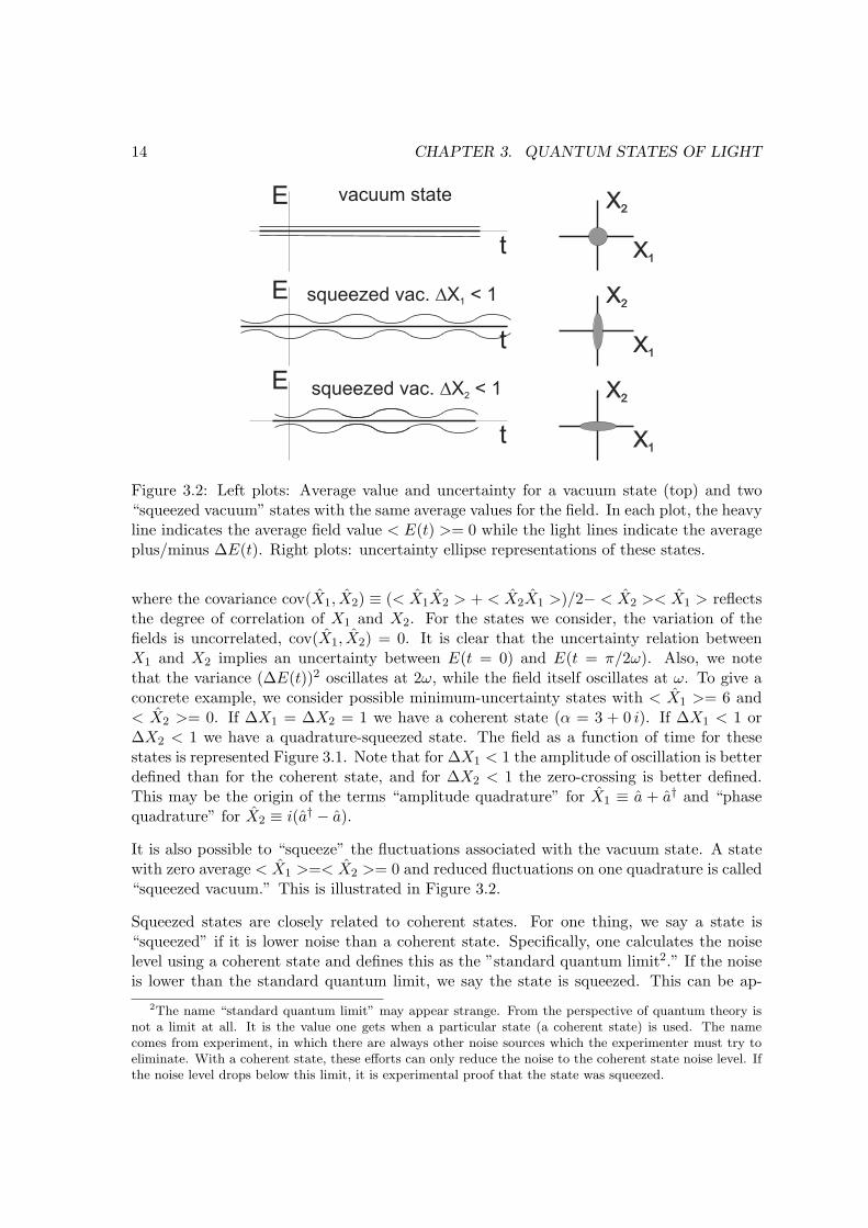
Figure 3.2: Left plots: Average value and uncertainty for a vacuum state (top) and two“squeezed vacuum” states with the same average values for the field. In each plot, the heavyline indicates the average field value < E(t) >= 0 while the light lines indicate the averageplus/minus ∆E(t). Right plots: uncertainty ellipse representations of these states.
where the covariance cov(X1, X2) ≡ (< X1X2 > + < X2X1 >)/2− < X2 >< X1 > reflectsthe degree of correlation of X1 and X2. For the states we consider, the variation of thefields is uncorrelated, cov(X1, X2) = 0. It is clear that the uncertainty relation betweenX1 and X2 implies an uncertainty between E(t = 0) and E(t = π/2ω). Also, we notethat the variance (∆E(t))2 oscillates at 2ω, while the field itself oscillates at ω. To give aconcrete example, we consider possible minimum-uncertainty states with < X1 >= 6 and< X2 >= 0. If ∆X1 = ∆X2 = 1 we have a coherent state (α = 3 + 0 i). If ∆X1 < 1 or∆X2 < 1 we have a quadrature-squeezed state. The field as a function of time for thesestates is represented Figure 3.1. Note that for ∆X1 < 1 the amplitude of oscillation is betterdefined than for the coherent state, and for ∆X2 < 1 the zero-crossing is better defined.This may be the origin of the terms “amplitude quadrature” for X1 ≡ a + a† and “phasequadrature” for X2 ≡ i(a† − a).
It is also possible to “squeeze” the fluctuations associated with the vacuum state. A statewith zero average < X1 >=< X2 >= 0 and reduced fluctuations on one quadrature is called“squeezed vacuum.” This is illustrated in Figure 3.2.
Squeezed states are closely related to coherent states. For one thing, we say a state is“squeezed” if it is lower noise than a coherent state. Specifically, one calculates the noiselevel using a coherent state and defines this as the ”standard quantum limit2.” If the noiseis lower than the standard quantum limit, we say the state is squeezed. This can be ap-
2The name “standard quantum limit” may appear strange. From the perspective of quantum theory isnot a limit at all. It is the value one gets when a particular state (a coherent state) is used. The namecomes from experiment, in which there are always other noise sources which the experimenter must try toeliminate. With a coherent state, these efforts can only reduce the noise to the coherent state noise level. Ifthe noise level drops below this limit, it is experimental proof that the state was squeezed.
3.4. COHERENT STATES 15
X1
X2
X1
X2
e-r
1
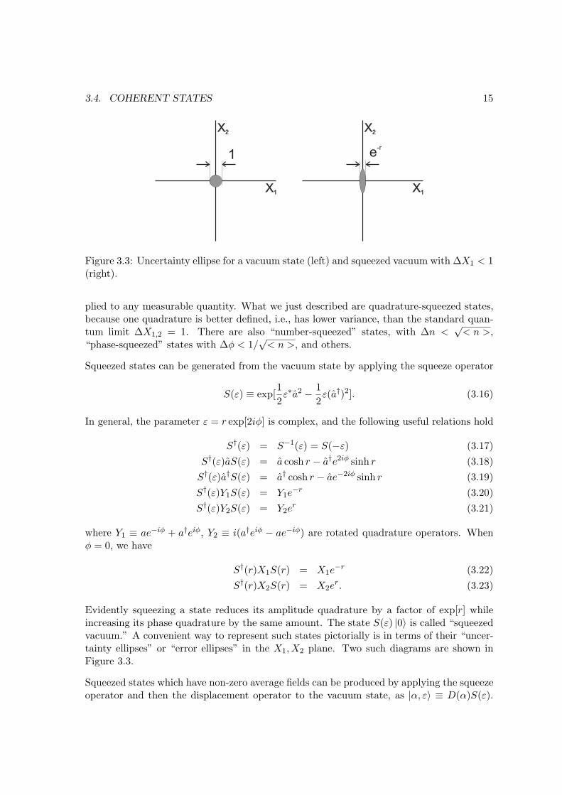
Figure 3.3: Uncertainty ellipse for a vacuum state (left) and squeezed vacuum with ∆X1 < 1(right).
plied to any measurable quantity. What we just described are quadrature-squeezed states,because one quadrature is better defined, i.e., has lower variance, than the standard quan-tum limit ∆X1,2 = 1. There are also “number-squeezed” states, with ∆n <
√< n >,
“phase-squeezed” states with ∆φ < 1/√
< n >, and others.
Squeezed states can be generated from the vacuum state by applying the squeeze operator
S(ε) ≡ exp[12ε∗a2 − 1
2ε(a†)2]. (3.16)
In general, the parameter ε = r exp[2iφ] is complex, and the following useful relations hold
S†(ε) = S−1(ε) = S(−ε) (3.17)S†(ε)aS(ε) = a cosh r − a†e2iφ sinh r (3.18)
S†(ε)a†S(ε) = a† cosh r − ae−2iφ sinh r (3.19)S†(ε)Y1S(ε) = Y1e
−r (3.20)S†(ε)Y2S(ε) = Y2e
r (3.21)
where Y1 ≡ ae−iφ + a†eiφ, Y2 ≡ i(a†eiφ − ae−iφ) are rotated quadrature operators. Whenφ = 0, we have
S†(r)X1S(r) = X1e−r (3.22)
S†(r)X2S(r) = X2er. (3.23)
Evidently squeezing a state reduces its amplitude quadrature by a factor of exp[r] whileincreasing its phase quadrature by the same amount. The state S(ε) |0〉 is called “squeezedvacuum.” A convenient way to represent such states pictorially is in terms of their “uncer-tainty ellipses” or “error ellipses” in the X1, X2 plane. Two such diagrams are shown inFigure 3.3.
Squeezed states which have non-zero average fields can be produced by applying the squeezeoperator and then the displacement operator to the vacuum state, as |α, ε〉 ≡ D(α)S(ε).
16 CHAPTER 3. QUANTUM STATES OF LIGHT
X1
X2
X1
X2
2a 2a
e-r
1
Figure 3.4: Uncertainty areas of a coherent state (left) and a bright squeezed state with∆X1 < 1 (right).
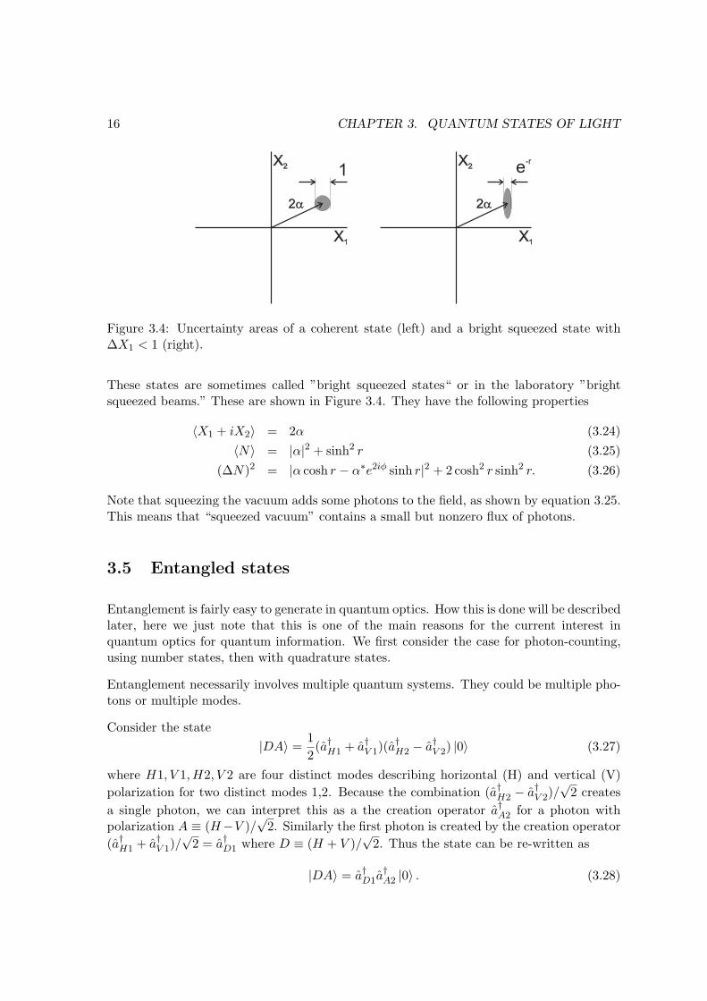
These states are sometimes called ”bright squeezed states“ or in the laboratory ”brightsqueezed beams.” These are shown in Figure 3.4. They have the following properties
〈X1 + iX2〉 = 2α (3.24)〈N〉 = |α|2 + sinh2 r (3.25)
(∆N)2 = |α cosh r − α∗e2iφ sinh r|2 + 2 cosh2 r sinh2 r. (3.26)
Note that squeezing the vacuum adds some photons to the field, as shown by equation 3.25.This means that “squeezed vacuum” contains a small but nonzero flux of photons.
3.5 Entangled states
Entanglement is fairly easy to generate in quantum optics. How this is done will be describedlater, here we just note that this is one of the main reasons for the current interest inquantum optics for quantum information. We first consider the case for photon-counting,using number states, then with quadrature states.
Entanglement necessarily involves multiple quantum systems. They could be multiple pho-tons or multiple modes.
Consider the state|DA〉 =
12(a†H1 + a†V 1)(a
†H2 − a†V 2) |0〉 (3.27)
where H1, V 1,H2, V 2 are four distinct modes describing horizontal (H) and vertical (V)polarization for two distinct modes 1,2. Because the combination (a†H2 − a†V 2)/
√2 creates
a single photon, we can interpret this as a the creation operator a†A2 for a photon withpolarization A ≡ (H−V )/
√2. Similarly the first photon is created by the creation operator
(a†H1 + a†V 1)/√
2 = a†D1 where D ≡ (H + V )/√
2. Thus the state can be re-written as
|DA〉 = a†D1a†A2 |0〉 . (3.28)
3.5. ENTANGLED STATES 17
This state simply describes two photons in two different modes, each with a different po-larization. If we write this the way it would be written in ordinary quantum mechanics, itwould be
|DA〉 = |D〉1 |A〉2 (3.29)
where |φ1,2〉1,2 is the state of the 1st or 2nd photon. This is a “product state.” In contrast,the state
∣∣Ψ−⟩=
1√2(a†H1a
†V 2 − a†V 1a
†H2) |0〉 =
1√2(|H〉1 |V 〉2 − |V 〉1 |H〉2) (3.30)
can not be factorized (written as a product) and is thus entangled. In fact, the state Ψ− iscalled a “Bell state” and it is often discussed in connection with quantum nonlocality andthe violation of Bell inequalities.
The above example shows entanglement in polarization, a discrete variable described interms of just two states H, V . Entanglement in continuous variables such as quadraturesis also possible. The best known example of this is the Einstein-Podolsky-Rosen (EPR)paradox, in which two particles have correlated positions x1−x2 = const. and anti-correlatedmomenta p1 + p2 = 0. The individual particles’ position and momentum are completelyuncertain, it is only the relative coordinate and combined momentum that are sharp. TheEPR situation can not be described by a product state of a wave-function for particle 1times a wave function for particle 2. More generally, it was shown by Duan, Giedke, Ciracand Zoller in 1999 that when the correlated variances are sufficiently small (∆(XA−XB))2+(∆(PA +PB))2 < 2, the state must be entangled, i.e., not factorizable. Here X, P are scaledvariables with the commutation relation [X, P ] = i.
It turns out that a state with EPR correlations in the quadratures of two different modesis also fairly easy to make in quantum optics. Again, we will show how to do this later,and for the moment we just show what such a state would look like. Consider the vacuumstate |0〉 of two different modes at frequencies ω+, ω−. Now squeeze this state using theunitary two-mode squeeze operator S2(G) = exp[G∗a+a− −Ga†+a†−]. The squeeze operatortransforms the annihilation operators as
S†2(G)a±S2(G) = a± cosh r − a†∓eiθ sinh r. (3.31)
To keep things simple, we take G = r exp[iθ] to be real, i.e. θ = 0. We define the sum anddifference quadratures
X1s ≡ (X1+ + X1−)/√
2 (3.32)X2d ≡ (X2+ − X2−)/
√2 (3.33)
and with a bit of algebra it can be shown that for the state S2(r) |0〉,(∆X1s)2 = e−2r (3.34)(∆X2d)2 = e−2r. (3.35)
This shows that it is possible to have a state of two modes which is squeezed in the sum ofthe amplitude quadratures and also in the difference of the phase quadratures. This same
18 CHAPTER 3. QUANTUM STATES OF LIGHT
state is anti-squeezed (variance larger than the coherent state value) for the difference ofthe amplitude quadratures and the sum of phase quadratures. A state like this can be usedto demonstrate continuous-variable entanglement by violating the inequality given by Duanet al. above.
This ends our sampling of the possible quantum states, but we have not exhausted thepossibilities. In fact the number of possible states grows exponentially with the number ofphotons (or the number of modes) available. Thus there are an infinitude of different states,and most of them have large numbers of photons and are not close to classical states. In asense, quantum optics is still just scratching the surface of the available quantum states. Asexperiments in optical quantum information advance, the states we use will become moreand more entangled, and less and less classical. Maybe some day the term “classical optics”will describe the unusual situation, rarely encountered, of an experiment that uses onlycoherent states.
Chapter 4
Detection of light
There are two principal ways of detecting light that are used in quantum optics. One,“direct detection,” detects the energy falling on a detector, and is closely related to thenumber-state basis, because this is the energy basis. The other method is to mix the signalbeam with a strong reference of the same wavelength and definite phase. The interferenceis detected as a power difference at the outputs of the beam-splitter. This depends on thephase of the measured beam, and the result is detection of a single quadrature. Naturally,such experiments are best explained using quadratures.
4.1 Direct detection and photon counting
The simplest method of detecting light, called “direct detection,” is to absorb the light onthe surface of a detector of some sort (a photodiode, a photomultiplier tube, a thermaldetector, etc.). The detector produces an electrical signal proportional to the power of theincident light. Classically, such a detector is called a “square-law” detector because theelectrical signal (voltage or current) is proportional to the square of the incident electricfield. Quantum mechanically, the signal indicates the number of photons that have beenabsorbed by the detector. If the detector is sensitive enough, individual photon arrivals canbe observed, and we speak of detection by “photon counting.”
The theory of photon counting was first presented by Roy Glauber in 1964 1. He notedthat while a classical photo-detection signal is proportional to the square of the electric fieldaveraged over a few cycles P (Class.)(t) ∝ ⟨
E2(t)⟩, the same can not be true for quantum
fields. In particular, because of vacuum fluctuations,⟨E2(t)
⟩> 0 even for the vacuum
state. If we naıvely applied the classical detection formula, it would imply detections even
1R. J. Glauber, Quantum Optics and Electronics, Les Houches Summer Lectures 1964, edited by C.DeWitt, A. Blandin, and C. Cohen-Tannoudji (Gordon and Breach, New York, 1965)
19
20 CHAPTER 4. DETECTION OF LIGHT
k
E
valenceband(filled)
conductionband(empty)
possibletransitions
= E/hbarw Di
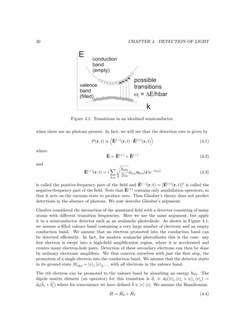
Figure 4.1: Transitions in an idealized semiconductor.
when there are no photons present. In fact, we will see that the detection rate is given by
P (r, t) ∝⟨E(−)(r, t) · E(+)(r, t)
⟩(4.1)
whereE = E(+) + E(−) (4.2)
and
E(+)(r, t) = i∑
k,α
√hωk
2ε0ak,αuk,α(r)e−iωkt (4.3)
is called the positive-frequency part of the field and E(−)(r, t) = [E(+)(r, t)]† is called thenegative-frequency part of the field. Note that E(+) contains only annihilation operators, sothat it acts on the vacuum state to produce zero. Thus Glauber’s theory does not predictdetections in the absence of photons. We now describe Glauber’s argument.
Glauber considered the interaction of the quantized field with a detector consisting of manyatoms with different transition frequencies. Here we use the same argument, but applyit to a semiconductor detector such as an avalanche photodiode. As shown in Figure 4.1,we assume a filled valence band containing a very large number of electrons and an emptyconduction band. We assume that an electron promoted into the conduction band canbe detected efficiently. In fact, for modern avalanche photodiodes this is the case: anyfree electron is swept into a high-field amplification region, where it is accelerated andcreates many electron-hole pairs. Detection of these secondary electrons can then be doneby ordinary electronic amplifiers. We thus concern ourselves with just the first step, thepromotion of a single electron into the conduction band. We assume that the detector startsin its ground state |0〉det = |v〉1 |v〉2 . . . with all electrons in the valence band.
The ith electron can be promoted to the valence band by absorbing an energy hωi. Thedipole matrix element (an operator) for this transition is di ≡ d0(|v〉i 〈c|i + |c〉i 〈v|i) =d0(bi + b†i ) where for convenience we have defined b ≡ |v〉 〈c|. We assume the Hamiltonian
H = H0 + HI (4.4)
4.1. DIRECT DETECTION AND PHOTON COUNTING 21
whereH0 =
∑
k
hωk(a†kak +
12) +
∑
i
hωib†i bi (4.5)
and
HI = −Ed
= −∑
i
(d0E
(+)b†i + d∗0E(−)bi
)−
∑
i
(d0E
(−)b†i + d∗0E(+)bi
)
≈ −∑
i
(d0E
(+)b†i + d∗0E(−)bi
). (4.6)
For clarity of presentation we assume just one polarization, and we drop the second sumbecause it greatly fails to conserve energy. Dropping this kind of term is known as the“rotating-wave approximation” and is discussed in greater detail in Chapter 10.
The detection rate for this model is calculated in detail in Appendix A, here we just givean outline. Treating HI as a perturbation, we first observe that to zero’th order the fieldE0(t) evolves under Maxwell’s equations from whatever is the initial conditions. Also underzero’th order, the probability of a given electron being excited
⟨b†ibi
⟩and the coherence
between valence and conduction states 〈bi〉 are zero. In second order time-dependent per-turbation theory, however, the probability of excitation grows as (Equation A.20)
d
dt〈ni(t)〉 =
|g|2h2
∫ t
0dt′
⟨E
(−)0 (t)E(+)
0 (t′)e−iωi(t−t′) + E(−)0 (t′)E(+)
0 (t)eiωi(t−t′)⟩
(4.7)
with |g|2 = |d0|2. When this is summed over all the electrons, which implies a sum over ωi.Converting this to an integral
∑i →
∫dωiρ(ωi) gives a delta-function 2πρδ(t− t′), so that
the rate of excitation becomesd
dt〈N(t)〉 ≡ d
dt
∑
i
〈ni〉 = 2πρ|g|2h2
⟨E
(−)0 (t)E(+)
0 (t)⟩
. (4.8)
This is Glauber’s result. To be clear, E0 is simply the field that enters the detector, as itwould evolve if the detector were not present. In this sense, it is an ideal measurement. Onthe other hand, the input field is consumed in the measurement, so it is very destructive!
A note of caution: the result above, P (t) ∝⟨E(−)(t)E(+)(t)
⟩or more generally P (x, t) ∝⟨
E(−)(x, t)E(+)(x, t)⟩
is used, implicitly or explicitly, to explain almost all photon-counting
experiments. In contrast, the proportionality constant 2πρ∣∣∣d0
h
∣∣∣2
is almost never used. Infact, it is not correct for most photon detectors. The expression was derived by pertur-bation theory, assuming that the probability of absorbing a photon was small. But mostoptical detectors are highly opaque to incident light. Roughly speaking, the expression
with 2πρ∣∣∣d0
h
∣∣∣2
is the absorption probability in the first thin slice of the detector, and theabsorption probability decays exponentially with depth beneath the surface. For an opaque,efficient detector, the sum of all the layers is one detection per incident photon. Typicallywe keep the result P (x, t) ∝
⟨E(−)(x, t)E(+)(x, t)
⟩, and find some other way to determine
the absolute rate of detections. For example, if somehow we know that the average powerfalling on the detector is Popt, then the average rate of detection is Popt/hω.
22 CHAPTER 4. DETECTION OF LIGHT
-
D1
D2
LO
in
Di(t)
f
Figure 4.2: Homodyne detection.
Coincidence counting
The expression above describes the detection probability for a single detector. What if thereare multiple detectors (almost always the case in photon counting experiments)? Then wemay be interested in correlations among the detections, for example, ”if detector A fires, sodoes detector B“ or ”detector A never fires exactly one nanosecond after detector B.”
Glauber also considered this situation. To see if two electrons have been excited, one ineach of detectors A, B, we calculate the evolution of the operator
N2(tA, tB) ≡∑
i,j
b†i (tA)b†j(tB)bj(tB)bi(tA) (4.9)
where the bi, bj act on electrons in detectors A,B. The probability density of seeing twodetections at times tA, tB is
P (tA, tB) =∂2
∂tA∂tB
⟨N2(tA, tB)
⟩(4.10)
and the perturbation calculation finds
P (tA, tB) ∝⟨E(−)(rA, tA)E(−)(rB, tB)E(+)(rB, tB)E(+)(rA, tA)
⟩. (4.11)
Note that the order of the operators is important. All of the annihilation operators are onthe right, so a state with insufficient photons (fewer than two in this case) is annihilated.The extension to N -photon detection is obvious.
4.2 Homodyne detection
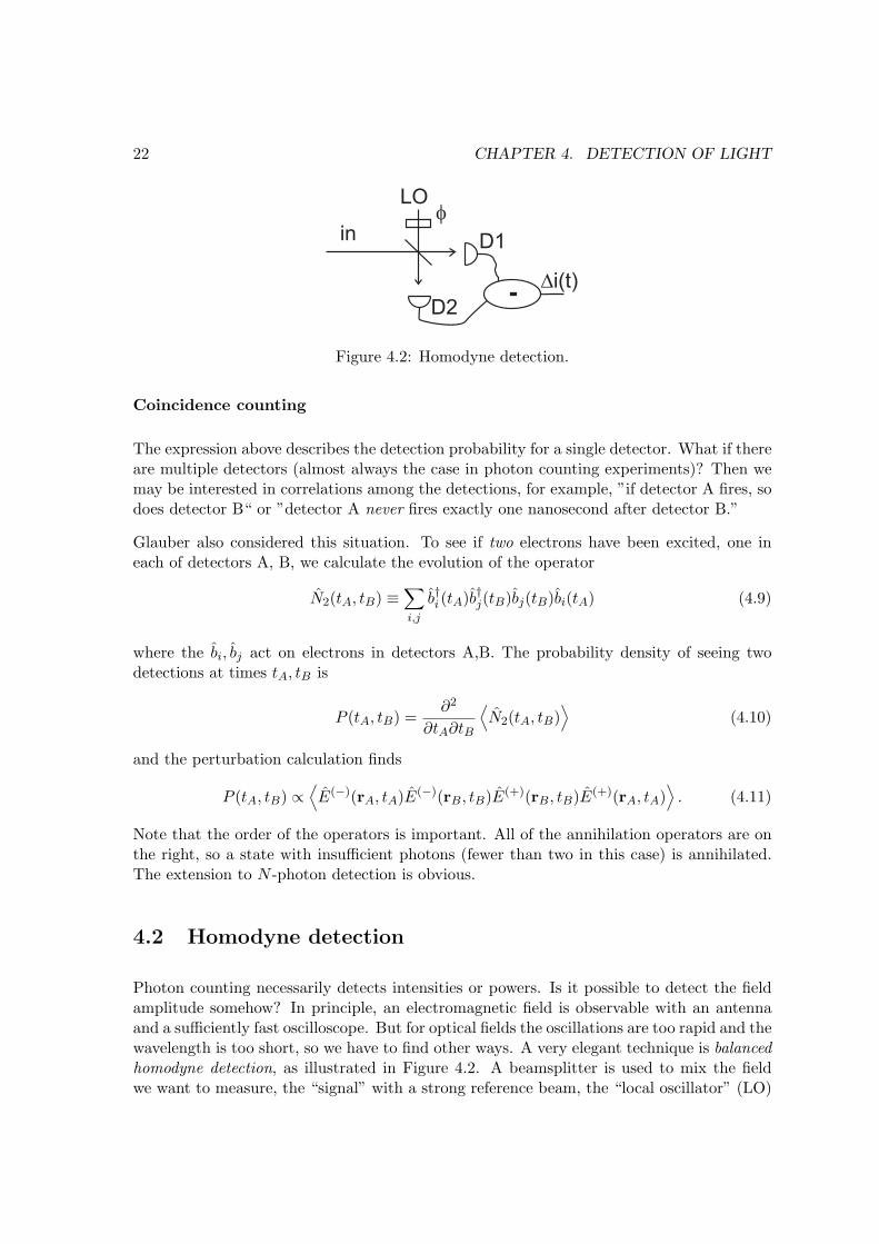
Photon counting necessarily detects intensities or powers. Is it possible to detect the fieldamplitude somehow? In principle, an electromagnetic field is observable with an antennaand a sufficiently fast oscilloscope. But for optical fields the oscillations are too rapid and thewavelength is too short, so we have to find other ways. A very elegant technique is balancedhomodyne detection, as illustrated in Figure 4.2. A beamsplitter is used to mix the fieldwe want to measure, the “signal” with a strong reference beam, the “local oscillator” (LO)
4.2. HOMODYNE DETECTION 23
whose phase φ we can control. We assume that the beamsplitter is balanced meaning thatthe transmission and reflection coefficients are equal magnitude. We also assume that theconditions for interference are ideal: the LO is in a single spatial mode, is monochromatic,and has a constant phase. Naturally, the input field must be matched to this mode. Ateach output port of the beamsplitter, a detector D1 or D2 detects all the light that leavesby that port. The photocurrents from these two detectors are immediately subtracted, sothat the output signal is ∆i(t) ∝ P1(t) − P2(t) where P1,2(t) are the powers arriving atdetectors D1 and D2.
We analyze the situation classically first. The LO field is ELO, the input field is Ein. Theyare assumed to have the same optical frequency ω. The fields leaving the beamsplitter are
E1 =1√2(ELO + Ein) (4.12)
E2 =1√2(ELO −Ein). (4.13)
The detected powers are
P1 ∝⟨E2
1
⟩=
12(⟨E2
LO
⟩+
⟨E2
in
⟩+ 2 〈ELOEin〉) (4.14)
P2 ∝⟨E2
2
⟩=
12(⟨E2
LO
⟩+
⟨E2
in
⟩− 2 〈ELOEin〉) (4.15)
where the brackets indicate time-averaging over several optical cycles. The subtraction ofthe signals gives
∆i(t) ∝ 〈ELO(t)Ein(t)〉 . (4.16)
It is clear already that this technique should be useful for the detection of weak fields: thesignal strength is proportional to 〈ELO(t)Ein(t)〉, much larger than than the signal strengthwith direct detection, proportional to 〈Ein(t)Ein(t)〉. Furthermore, in terms of quadratures,ELO(t) = X
(LO)1 sinωt−X
(LO)2 cosωt and Ein(t) = X
(in)1 sinωt−X
(in)2 cosωt, we have
∆i(t) ∝ X(LO)1 X
(in)1 + X
(LO)2 X
(in)2 . (4.17)
Represented in terms of phasors 2α = X1 + iX2 (these will later become coherent stateamplitudes), we find that
∆i(t) ∝ Re[α∗LOαin]. (4.18)
We note a few very attractive features of this measurement technique. As mentioned already,this offers a way to boost weak signals, by mixing them with a strong reference. This isthe basis of most techniques in radio transmission, for example. It also allows us to makequadrature measurements. For example, if we choose αLO to be real, so that X
(LO)2 = 0,
then the signal indicates only the real part of αin, or equivalently only the quadrature X(in)1 .
By changing the phase φ of the LO, we can measure X(in)1 , X
(in)2 , or any linear combination
(a generalized quadrature) X(in)1 sinφ + X
(in)2 cosφ. Finally, we note that the technique is
very favorable for low-noise measurements. Noise in the LO, for example if αLO = α0 + δα,
24 CHAPTER 4. DETECTION OF LIGHT
X1
X2
ELO
Ein
E1
E2
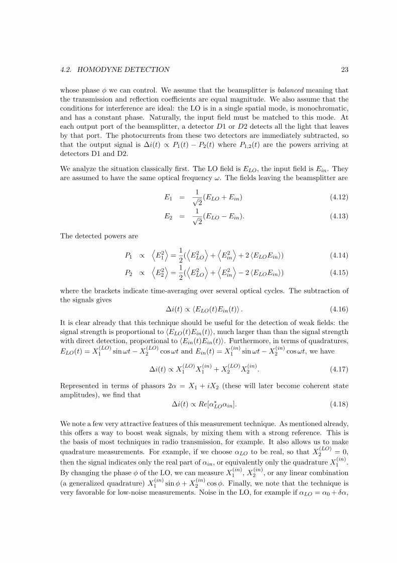
Figure 4.3: Phase-space representation of quadrature detection. A strong local oscillatorfield is mixed with the input signal, giving E1 = (ELO+Ein)/
√2 and E2 = (ELO−Ein)/
√2.
Curved lines show contours of constant power. The detected signal ∆i ∝< E21 > − < E2
2 >is a measure of one generalized quadrature of Ein, the one in-phase with ELO.
then δα contributes to the noise in the signal as δ∆i(t) ∝ Re[δα∗αin]. Because αin is small,noise in the LO has a small effect on the measurement noise. In the words of Hans Bachor,”This is an extremely useful and somewhat magical device.”
A pictorial representation of the homodyne measurement process is shown in Figure 4.3.
The quantum mechanical description of homodyne measurement is very simple, but assumesa quantum-mechanical understanding of beamsplitters that we will develop later. The resultof that understanding is that the beamsplitter transforms the quantum fields as
E1 =1√2(ELO + Ein) (4.19)
E2 =1√2(ELO − Ein). (4.20)
In other words, the quantum beamsplitter acts just like the classical one. The detectionprocess, treated quantum mechanically, gives the same results as the classical treatmentbecause when detected each beam contains many photons and is nearly classical. FollowingGlauber, we would write each photocurrent as
i1 ∝⟨E
(−)1 E
(+)1
⟩=
⟨E
(−)LO E
(+)LO + E
(−)in E
(+)in + E
(−)LO E
(+)in + E
(−)in E
(+)LO
⟩(4.21)
i2 ∝⟨E
(−)2 E
(+)2
⟩=
⟨E
(−)LO E
(+)LO + E
(−)in E
(+)in − E
(−)LO E
(+)in − E
(−)in E
(+)LO
⟩(4.22)
so that
∆i = i1 − i2 ∝⟨E
(−)LO E
(+)in + E
(−)in E
(+)LO
⟩∝ X
(LO)1 X
(im)1 + X
(LO)2 X
(im)2 . (4.23)
Note that to get this last expression we have used the fact that the LO field is single mode,so that E(+) ∝ ak = (X1 + iX2)/2 and that quadrature operators for the LO and input
4.2. HOMODYNE DETECTION 25
fields commute [X(LO)1 , X
(im)2 ] = 0. This gives us the same result as the classical case,
but now with the quantized quadrature operators. The rest of the discussion, about noisecontributions, signal strengths, etc. is the same.
26 CHAPTER 4. DETECTION OF LIGHT
Chapter 5
Correlation functions
Because many things that we measure in quantum optics are random (quantum noise,photon arrival times from stochastic sources, as well as ordinary noise from imperfect in-struments or environmental conditions), we often rely upon correlation functions to describeour results.
Classically, a correlation function is simply the average of a product of two or more quan-tities, for example the amplitude autocorrelation function is
G(1)(τ) ≡ 〈E(t)E(t + τ)〉 = limT→∞
1T
∫ T
0dt E(t)E(t + τ) (5.1)
and the amplitude cross-correlation function between fields EA and EB is
G(1)A,B(τ) ≡ 〈EA(t)EB(t + τ)〉 = lim
T→∞1T
∫ T
0dtEA(t)EB(t + τ). (5.2)
Correlation functions are, in general, expressions of the degree of coherence within a singlesource or between different sources. We illustrate by considering interference between twosources EA(t), EB(t) which we combine on a beamsplitter to produce the fields E1,2(t) ≡[EA(t) ± EB(t + τ)]/
√2. Here τ is a small variable delay that we can use to change the
relative phase of the fields. After the beamsplitter the fields are detected, giving currents
i1,2(τ) ∝⟨[EA(t)± EB(t + τ)]2
⟩/2 =
⟨E2
A
⟩/2 +
⟨E2
B
⟩/2± 〈EA(t)EB(t + τ)〉 (5.3)
ori1,2(τ) ∝
⟨E2
A
⟩+
⟨E2
B
⟩± 2G
(1)A,B(τ). (5.4)
Note that the interference signal comes entirely from the correlation function G(1)A,B(τ).
The autocorrelation function G(1)(τ) above is closely related to spectroscopy. We illustratewith an unbalanced Mach-Zehnder interferometer. The input field E(t) is split into twobeams which travel paths which differ in length by cτ . The beams are then combined on a
27
28 CHAPTER 5. CORRELATION FUNCTIONS
-
D1
D2
Di(t)
tNa
G ( )(1)
t
t
P( )n
n
P( )n
n
P( )n
n
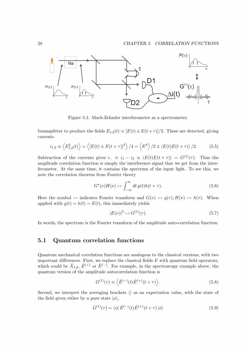
Figure 5.1: Mach-Zehnder interferometer as a spectrometer.
beamsplitter to produce the fields E1,2(t) ≡ [E(t)±E(t + τ)]/2. These are detected, givingcurrents
i1,2 ∝⟨E2
1,2(t)⟩
=⟨[E(t)±E(t + τ)]2
⟩/4 =
⟨E2
⟩/2± 〈E(t)E(t + τ)〉 /2. (5.5)
Subtraction of the currents gives i− ≡ i1 − i2 ∝ 〈E(t)E(t + τ)〉 = G(1)(τ). Thus theamplitude correlation function is simply the interference signal that we get from the inter-ferometer. At the same time, it contains the spectrum of the input light. To see this, wenote the correlation theorem from Fourier theory
G∗(ν)H(ν) ↔∫ ∞
−∞dt g(t)h(t + τ). (5.6)
Here the symbol ↔ indicates Fourier transform and G(ν) ↔ g(τ), H(ν) ↔ h(τ). Whenapplied with g(t) = h(t) = E(t), this immediately yields
|E(ν)|2 ↔ G(1)(τ). (5.7)
In words, the spectrum is the Fourier transform of the amplitude auto-correlation function.
5.1 Quantum correlation functions
Quantum mechanical correlation functions are analogous to the classical versions, with twoimportant differences. First, we replace the classical fields E with quantum field operators,which could be X1,2, E(+) or E(−). For example, in the spectroscopy example above, thequantum version of the amplitude autocorrelation function is
G(1)(τ) ≡⟨E(−)(t)E(+)(t + τ)
⟩. (5.8)
Second, we interpret the averaging brackets 〈〉 as an expectation value, with the state ofthe field given either by a pure state |φ〉,
G(1)(τ) = 〈φ| E(−)(t)E(+)(t + τ) |φ〉 (5.9)
5.2. INTENSITY CORRELATIONS 29
or a density matrix ρG(1)(τ) = Tr[ρE(−)(t)E(+)(t + τ)]. (5.10)
Note that in many cases the averaging brackets imply both an expectation value and a timeaverage. This is the case in the above expressions, where the average over t is implied bythe fact that G(1)(τ) does not contain t. As an example of the other sort, recall that inGlauber’s photodetection theory the probability density of detecting a photon at time t was
P (t) ∝⟨E(−)(t)E(+)(t)
⟩. (5.11)
5.2 Intensity correlations
As noted already, field correlation functions such as G(1)(τ) are important in classical opticsfor describing partial coherence. In contrast, intensity correlation functions appear muchless commonly. Nevertheless, they have been important in astronomy, where R. Hanbury-Brown was able to measure the diameters of stars using intensity correlations in radiosignals.
Classically, an intensity cross-correlation function between two signals A and B is
G(2)A,B(τ) ≡ 〈IA(t)IB(t + τ)〉 . (5.12)
If the two sources are correlated, then G(2)A,B(0) > 〈IA〉 〈IB〉, while if they are uncorrelated,
G(2)A,B(0) = 〈IA〉 〈IB〉. Hanbury-Brown used two radio-telescopes pointed to the same star
to collect the intensities IA, IB. When the telescopes were sufficiently close to each other,i.e., within a coherence length, the intensities were strongly correlated. When they wereseparated by more than a coherence length, the correlations dropped off. This way Hanbury-Brown was able to measure the coherence length and thus the angular size of the stars.Practically, it was much easier to measure G
(2)A,B(0) than an amplitude correlation function,
because there was no need to preserve the phase of the rapidly-varying radio fields. It wassufficient to detect and multiply intensities, which were relatively slowly varying.
Intensity correlations play a very important role in quantum optics, especially in photon-counting experiments. From Glauber’s theory, a product of four operators describes theprobability density for coincidence detection of two photons
P (tA, tB) ∝⟨E
(−)A (tA)E(−)
B (tB)E(+)B (tB)E(+)
A (tA)⟩
. (5.13)
If we define tA ≡ t and tB ≡ t + τ and average this expression over t we get the probabilityfor seeing a pair of detections separated by a time τ
G(2)A,B(τ) ≡
⟨E
(−)A (t)E(−)
B (t + τ)E(+)B (t + τ)E(+)
A (t)⟩
. (5.14)
A special case is when A and B are copies of the same field, for example if a single beam issplit to two detectors by a beamsplitter. Then we have
G(2)(τ) ≡⟨E(−)(t)E(−)(t + τ)E(+)(t + τ)E(+)(t)
⟩. (5.15)
30 CHAPTER 5. CORRELATION FUNCTIONS
Finally, we note that the various G functions we have written all have units of some sort.It is often convenient to work with normalized correlation functions, for example
g(2)(τ) ≡⟨E(−)(t)E(−)(t + τ)E(+)(t + τ)E(+)(t)
⟩
⟨E(−)(t)E(+)(t)
⟩2 =G(2)(τ)〈I〉2 . (5.16)
This last function, g(2)(τ), appears in so many important experiments, it can be called“gee-2” without risk of confusion.
5.3 Measuring correlation functions
Measuring correlation functions in the laboratory is straightforward. We consider as anexample the measurement of g(2)(0) and distinguish a couple of measurement scenarios.If the detectors are unable to resolve individual photon arrivals, either because there aretoo many, or because the detector noise is too large, then we must consider the signals tobe continuous. The detectors produce photocurrents i1,2(t) ∝ I1,2(t) (plus detector noise).Analog electronic circuits are then used to delay i1, multiply i1×i2, and average the productto obtain a signal proportional to 〈I1(t)I2(t + τ)〉. If the noise in the two detectors is uncor-related, it makes no contribution to this average. The individual intensities 〈I1(t)〉 , 〈I2(t)〉in g(2) usually do not need to be measured directly. It is almost always the case that I1(t)and I2(t + τ) are uncorrelated for suitably large τ . In this case, 〈I1(t)I2(t + τ)〉→ 〈I1〉 〈I2〉.Alternately, each photocurrent can be recorded with a fast oscilloscope and the correlationfunctions computed afterward.
In the case where single-photon counting is used, we have to make allowance for the factthat the signals are discrete: the photons arrive at times t1, t2, etc. In principle we coulddescribe the power P (t) reaching the detector as a series of delta functions P (t) = AI(t) =hω[δ(t− t1) + δ(t− t2) + . . .], where A is the area of the detector. But delta functions arenot what we measure in the laboratory, since we never have infinite time-resolution in ourmeasurements. Instead, we divide the time into intervals, called “bins,” of duration δt, i.e.,bk : kδt ≤ t < (k + 1)δt. The experimental signal is the number of detections in each timebin, nk, proportional to the integrated power nk =
∫t∈bk
dt P (t)/hω. Our best estimate ofthe intensity is “coarse-grained”: I(t) ∝ ni, i = bt/δtc. The integrals in the correlationfunction now become sums, for example
〈I(t)I(t + jδt)〉 =1T
∫ T
0dt I(t)I(t + jδt) =
1N
h2ω2
A2
N∑
i
nini+j ∝ 〈nini+j〉 . (5.17)
As with continuous signals, one strategy is to simply record the detector output. Each timea photon arrives the time of the detector’s firing is recorded, so that ni = 1 for those timebins and ni = 0 for all others. This strategy is called “time-stamping” because each photonarrival time is “stamped” into the memory of a computer somewhere. Correlation functions(to any order) can then be calculated later.
5.3. MEASURING CORRELATION FUNCTIONS 31
A more common strategy is to compute the correlation function electronically, using coinci-dence counting techniques, also known as “time-correlated photon counting.” For example,the photodiode signal can be used to start a timer (a time-to-amplitude converter or time-to-digital converter), and the next signal used to stop the timer. The timer value is thenrecorded by a computer or multi-channel analyzer, and the process is repeated. A his-togram of the time differences is proportional to
⟨nini+τ/δt
⟩, assuming 1) ni ≤ 1 and 2)
〈n〉 τ/δt ¿ 1. This second restriction arises because the timer counts only until the firststop event. More sophisticated, “multi-stop” counters can circumvent this problem.
When two or more detectors are used and we count only pairs (or trios, quartets, etc.) ofphotons that arrive in the same time bin, we talk of “coincidence detection” and ”coincidencecounting.” This gives a signal proportional to 〈nA,inB,i〉 and can be implemented with verysimple electronics, often nothing more than AND gates and inexpensive counters.

32 CHAPTER 5. CORRELATION FUNCTIONS
Chapter 6
Representations of quantum statesof light
6.1 Introduction
So far, the states of the field we have considered, number states, vacuum, coherent states,squeezed states, are all pure states. In this section we develop several ways to describemixed states in quantum optics. As in quantum mechanics, a mixed state is described by adensity operator. Unlike most problems in quantum mechanics, we will find that althoughthe density matrix exists, is not the most useful representation for many situations. Wewill thus develop representations of the density operator in terms of continuous degrees offreedom such as the quadratures X1, X2. These will be phase space distributions.
It turns out that there are many phase space distributions, and we will only be able tomention the most common ones. For a more complete treatment, we recommend the booksby Scully and Zubairy, and by Walls and Milburn, and references therein.
6.2 Density operator
A mixed state is described by its density operator
ρ ≡∑
wi |ψi〉 〈ψi| (6.1)
where |ψi〉 are normalized states and wi ≥ 0 and∑
i wi = 1. Thus {wi} can be interpretedas a probabilities: wi is the probability that the system is prepared in the state |φi〉. Theexpectation value of an operator A is
〈A〉 = Tr[ρA] ≡∑
j
〈φj | ρA |φj〉 (6.2)
33
34 CHAPTER 6. REPRESENTATIONS OF QUANTUM STATES OF LIGHT
where {|φj〉} is a set of basis states. It follows that
Tr[ρA] =∑
i
wi 〈ψi|A |ψi〉 . (6.3)
This describes an incoherent addition of the contributions from each |ψi〉.
6.3 Representation by number states
The density operator can be expanded in terms of number states as
ρ =∑
n,n′ρn,n′ |n〉
⟨n′
∣∣ (6.4)
where density matrix isρn,n′ ≡ 〈n| ρ ∣∣n′⟩ . (6.5)
Note that this simple relationship is possible because∑n
|n〉 〈n| = I. (6.6)
Not all expansions that we use will have this nice property.
This representation contains all the information about the state, and is simple to interpret.For example the diagonal element ρn,n is the probability to have n photons in the state,while the off-diagonal element ρ0,1 is the coherence between the n = 0 and n = 1 parts ofthe state.
This representation is useful for fields with a definite extent in space or in time. Forexample, for fields within a cavity (as in the Jaynes-Cummings model), or to characterizethe total (i.e. integrated) field in a pulse. But there are many situations in which countingthe number of photons is not natural, for example the field emitted by a continuous-wavelaser. Also, while there are good techniques for measuring the diagonal elements (photoncounting), it is not so easy to measure the off-diagonal elements. For these reasons, we needother representations.
6.4 Representation in terms of quadrature states
The density operator can be expanded in terms of quadrature states as
ρ =∫
dX1 dX ′1 |X1〉 〈X1| ρ
∣∣X ′1
⟩ ⟨X ′
1
∣∣ =∫
dX1 dX ′1 g(X1, X
′1) |X1〉
⟨X ′
1
∣∣ (6.7)
where
g(X1, X′1) ≡ 〈X1| ρ
∣∣X ′1
⟩=
∑
i
wi 〈X1|ψi〉⟨ψi|X ′
1
⟩=
∑
i
wiψi(X1)ψ∗i (X′1) (6.8)
6.5. REPRESENTATIONS IN TERMS OF COHERENT STATES 35
and ψi(X1) ≡ 〈X1|ψi〉. Clearly a similar expression could be written for expansion inX2 or any generalized quadrature. This representation has the advantage of being closelyconnected to the wave-functions ψi(X1), and thus may be more intuitive than other rep-resentations. But in fact it is almost never used in quantum optics, because an equivalentrepresentation, the Wigner distribution (described below), is more symmetric, is easier tointerpret, and is easier to measure.
6.5 Representations in terms of coherent states
Consider an expansion of the density operator in coherent states
ρ =∫
d2α d2α′ f(α, α′) |α〉 ⟨α′
∣∣ (6.9)
where α ≡ x1 + ix2 = r exp[iφ] and thus d2α = dx1dx2 = rdrdφ 1. The function f isanalogous to the density matrix, and the expansion is always possible due to the over-completeness of the coherent states. I.e., there is always a function f which satisfies this.For example,
f(α, α′) =1π2〈α| ρ ∣∣α′⟩ (6.10)
satisfies Equation (6.9), which is easily shown using the identity
1π
∫d2α |α〉 〈α| = I. (6.11)
But this solution is not unique. For example, for the pure coherent state ρ = |β〉 〈β|, onesolution is f(α, α′) = 〈α|β〉 〈β|α′〉 /π2 = exp[−|α−β|2/2+α∗β] exp[−|α′−β|2/2+α′β∗]/π2
and another solution is f ′(α, α′) = δ2(α−β)δ2(α′−β). This suggests that this representationsomehow has too many degrees of freedom. At the same time, we know from the expansionin quadrature states that the density operator can represented by a function of just tworeal variables, while the function f depends on four. This motivates us to look for lower-dimensional representations of the density operator.
6.5.1 Glauber-Sudarshan P-representation
If we assume that the f function above is diagonal, i.e. f(α, α′) = P (α)δ2(α−α′), then wehave the expansion
ρ =∫
d2α d2α′ f(α, α′) |α〉 ⟨α′
∣∣ =∫
d2α P (α) |α〉 〈α| . (6.12)
This representation was introduced independently by Glauber and Sudarshan, and is calledthe Glauber-Sudarshan P-representation or simply the P-representation. It can be shown
1This expansion is very similar to one considered by Glauber, namely ρ =1
π2
∫d2α d2β R(α∗, β) |α〉 〈β| exp[−(|α|2 + |β|2)/2] where R(α∗, β) = 〈α| ρ |β〉 exp[(|α|2 + |β|2)/2].
36 CHAPTER 6. REPRESENTATIONS OF QUANTUM STATES OF LIGHT
that
Tr[ρ] = 1 =∫
d2α P (α). (6.13)
The function P (α) can sometimes be thought of as a probability distribution, and the stateas a mixture of coherent states. This is possible when P (α) ≥ 0 for all α, but for somestates this is not the case. For example, for squeezed states P is negative in some regions.For n > 0 number states, P does not exist, at least not as a regular function. But when itP does exist, it is uniquely determined by ρ.
6.5.2 Husimi distribution or Q-representation
Another representation of the state is
Q(α) ≡ 1π〈α| ρ |α〉 . (6.14)
Apart from a factor of π, this is the diagonal element of the function f(α, α′) = 〈α| ρ |α′〉 /π2.It can be shown that ∫
d2α Q(α) = 1 (6.15)
and clearly Q(α) is positive definite. Note that Q does not describe an expansion of thestate, i.e., ρ 6= ∫
d2α Q(α) |α〉 〈α|. Nevertheless, Q(α) determines uniquely the state ρ.
6.6 Wigner-Weyl distribution
The Wigner-Weyl distribution, also called the Wigner distribution and the Wigner function,is similar in many ways to the P- and Q-representations. Its shape in phase-space is some-where between the two. Its mathematical definition is more complicated than the P- andQ-distributions’, and because of this the Wigner function often seems rather mysterious.Nevertheless, it will be worth knowing because:
1) It exists for any state.2) It corresponds to the classical phase-space distribution.3) It has a Fourier-transform relationship to the density operator (in the quadrature repre-sentation).4) It correctly predicts marginal distributions.5) It can be measured (indirectly).
To introduce the Wigner function, we start with some classical statistics.
6.6. WIGNER-WEYL DISTRIBUTION 37
6.6.1 Classical phase-space distributions
In classical physics, an individual system follows a trajectory through phase space, definedby the evolution of the coordinates and momenta, e.g., q(t), p(t). It is also possible todescribe an ensemble of such systems behaving in a statistical manner, such that a functionF (q, p) describes the probability to find the system near to q, p, i.e., the probability to bein the range q to q + dq and p to p + dp is F (q, p)dq dp. This probability density F is aphase-space distribution. Some characteristics of such a distribution are: non-negativityF ≥ 0, normalization
∫dq dp F (q, p) = 1. The marginal distributions F (q) ≡ ∫
dpF (q, p)and F (p) ≡ ∫
dq F (q, p) give the probability density for a single coordinate or momentum,averaging over the possible values of the other degree of freedom. This generalizes in theobvious way to more coordinates and momenta.
For a classical harmonic oscillator, the direct method to measure F (x, p) is by repeatedlypreparing the state and measuring simultaneously x and p. After many measurementsit is possible to estimate F (x, p). There are also indirect methods, which do not requiresimultaneous measurement of x and p. One way to do this is by measuring the characteristicfunction for the state.
In classical statistics, a characteristic function χ(k) is defined as the expectation value ofthe random variable exp[ikx], where x itself is a random variable and k is a parameter.This can be calculated for any random variable x. For example, if x were the arrival timeof your morning train, over the course of a year you could sample x 365 times, and thenestimate 〈exp[ikx]〉 ≈ (exp[ikx1] + exp[ikx2] + . . .)/365. And of course, you can calculatethis for any value of k you like.
If F (x) is the distribution function (or probability density function) for x, then
χ(k) =⟨eikx
⟩=
∫dxF (x)eikx. (6.16)
In multiple dimensions, this is generalized to
χ(k) =⟨eik·x
⟩=
∫dnxF (x)eik·x. (6.17)
Thus the characteristic function is nothing more than the (inverse) Fourier transform of thedistribution function. Note that for any given k, χ(k) can be estimated by measurementsof just one component of x, the component parallel to k. If this component can be directlymeasured, then no simultaneous measurements are required. The characteristic function isuseful in statistics for the usual reasons, e.g., a convolution of distribution functions can becomputed using the product of their characteristic functions.
6.6.2 Applying classical statistics to a quantum system
For a quantum system, direct measurement of the distribution function is not possible,because simultaneous measurement of X1 and X2 is forbidden by the uncertainty principle.
38 CHAPTER 6. REPRESENTATIONS OF QUANTUM STATES OF LIGHT
The characteristic function, in contrast, can be measured. For example, if we want tomeasure
χ(k) =⟨eik·X
⟩(6.18)
for some particular value of k, where k ≡ (k1, k2) ≡ (k cos θ, k sin θ) and X = (X1, X2),then we have
χ(k) =⟨eik(X1 cos θ+X2 sin θ)
⟩=
⟨eikXθ
⟩(6.19)
where Xθ = X1 cos θ +X2 sin θ is a generalized quadrature. The value of χ(k) can be deter-mined by measuring Xθ several times, for example in a balanced homodyne measurement,and then computing the average
⟨eikXθ
⟩. This does not conflict with the uncertainty prin-
ciple, because we only measure one quadrature at a time. By repeating this with severalvalues of θ, it is possible to build up an approximation of χ(k). From quantum theory, weknow that the expectation value is
⟨eikXθ
⟩= Tr[ρ exp[ikXθ]], so that
χ(k) = Tr[ρeik·X]. (6.20)
It is then possible to calculate a distribution function W (x1, x2) as the Fourier transformof χ. Note that in W (x1, x2), x1, x2 are real-valued parameters of the function W , notoperators. Also, note that k ·X = (k1 + ik2)a† + (k1 − ik2)a. The distribution function isthen
W (x1, x2) = F [χ(k1, k2)] =1
4π2
∫dk1 dk2 e−ik·x Tr
[ρeik·X
]
=1
4π2
∫dk1 dk2 e−ik·x Tr
[ρei[(k1+ik2)a†+(k1−ik2)a]
]. (6.21)
We are almost finished. It only remains to put this in the usual form. We note that if2α = x1 + ix2 and β = k1 + ik2, then αβ∗ + α∗β = x1k1 + x2k2 and the Fourier transformcan be written equivalently
W (x1, x2) = F [χ(k1, k2)] =1
4π2
∫dk1 dk2 e−ik1x1−ik2x2χ(k1, k2)
W (α) = F [χ(β)] =1π2
∫d2β e−i(αβ∗+α∗β)χ(β) (6.22)
whereχ(β) = Tr
[ρei(βa†+β∗a)
]. (6.23)
This agrees with the convention used by Scully and Zubairy. Other authors may define βdifferently, for example it is common to use β′ ≡ (−k2 + ik1)/2 = iβ, so that the Fouriertransform is ∝ ∫
d2β′ exp[αβ′∗ − α∗β′]χ′(β′) and the characteristic function is χ′(β′) =⟨exp[β′a† − β′∗a]
⟩. 2. We have used the symbol W (α), because this in fact is our definition
of the Wigner distribution: the Fourier transform of the characteristic function χ.2The usual form for the Wigner function in quantum optics makes it look as much as possible like the P
and Q distributions. For example the quadratures x1, x2 are organized into a single complex amplitude α as ifthey were a coherent state. This is elegant but perhaps misleading. There are no coherent states used in thedefinition of the Wigner function, and it is not related to expansion of ρ in coherent states. W is also moregeneral than the P and Q distributions. You can define a Wigner function for other coordinate/momentumpairs, e.g. angle and angular momentum, for which coherent states do not exist and thus P and Q are notdefined.
6.6. WIGNER-WEYL DISTRIBUTION 39
It is worth re-stating how we derived the Wigner distribution, to highlight what is classicaland what is quantum about it. W is the Fourier transform of the characteristic function,which in classical statistics is the (inverse) Fourier transform of the distribution F , so clas-sically we would have the trivial relationship W = F [F−1[F ]] = F . In Quantum mechanicswe do not have a distribution F , but we have the density operator ρ, which predicts allmeasurements we can make, including χ, which plays the role of F−1[F ] (classically it isF−1[F ]). The quantum ingredient is the measurement outcomes (and the way of predictingthem), but the statistical treatment is completely classical.
6.6.3 Facts about the Wigner distribution
The Wigner distribution is normalized, in the sense that∫
W (x1, x2)dx1dx2 =14W (α)d2α = Tr[ρ]. (6.24)
The Wigner distribution is real. The Wigner distribution can be used to calculate theoverlap or fidelity of two states, in the sense that if W,W ′ are the Wigner distributions forstates ρ, ρ′, respectively, then
∫W (x1, x2)W ′(x1, x2)dx1dx2 =
14π
Tr[ρρ′]. (6.25)
Marginal distributions
For any ρ, measurements of the quadrature X1 will have a probability distribution
P (x1) = Tr[ρ |x1〉 〈x1|] (6.26)
where |x1〉 〈x1| is a projector onto the X1 eigenstate X1 |x1〉 = x1 |x1〉. As with positioneigenstates, the eigenstates |x1〉 are not normalized, but the projectors are, in a sense:
∫dx1 |x1〉 〈x1| = I, (6.27)
where I is the identity operator. More abstractly, we can write |x1〉 〈x1| = δ(X1 − x1).
We now calculate P (x1) as a marginal distribution. That is, we integrate W over the othercoordinates (only x2 in this case) and find
∫dx2 W (x1, x2) =
14π2
∫dx2
∫dk1 dk2 e−ik1x1−ik2x2χ(k1, k2)
=12π
∫dk1 dk2 δ(k2)e−ik1x1χ(k1, k2)
=12π
∫dk1 e−ik1x1χ(k1, 0)
=12π
∫dk1 e−ik1x1Tr[ρeik1X1 ]
= Tr[ρδ(X1 − x1)] = P (x1). (6.28)
40 CHAPTER 6. REPRESENTATIONS OF QUANTUM STATES OF LIGHT
This confirms our earlier claim, that W is like the probability distribution F ; it can be usedto calculate the probability for an observable simply by integrating over (”tracing over”)the other observables.
To find the distribution for a generalized quadrature Xθ = X1 cos θ + X2 sin θ, we definerotated coordinates xθ, xθ through
x1 = xθ cos θ − xθ sin θ
x2 = xθ sin θ + xθ cos θ (6.29)
so that∫
dxθ W (x1, x2) =∫
dxθ W (xθ cos θ − xθ sin θ, xθ sin θ + xθ cos θ)
= Tr[ρδ(Xθ − xθ)] = Pθ(xθ). (6.30)
6.6.4 “Characteristic functions” for Q- and P-distributions
We can generalize the above mathematics (but not it’s interpretation!) to include the P- andQ-distributions. In particular, we can identify three versions of the characteristic function.The one we defined above is called the symmetrically-ordered characteristic function
C(β) ≡⟨ei(aβ∗+a†β)
⟩= Tr[ρei(aβ∗+a†β)] = χ(β). (6.31)
The other two are the normally-ordered (N) and anti-normally-ordered (A) characteristicfunctions
CN (β) ≡⟨eia†βeiaβ∗
⟩= Tr[ρeia†βeiaβ∗ ] (6.32)
andCA(β) ≡
⟨eiaβ∗eia†β
⟩= Tr[ρeiaβ∗eia†β]. (6.33)
If we now take the Fourier transforms of these characteristic functions, we will have threedistributions, which are equal to W,P, and Q.
W (α) ≡ 1π2
∫d2β e−i(αβ∗+α∗β)C(β) (6.34)
P (α) ≡ 1π2
∫d2β e−i(αβ∗+α∗β)CN (β) (6.35)
Q(α) ≡ 1π2
∫d2β e−i(αβ∗+α∗β)CA(β) (6.36)
These characteristic functions are useful for proving things about the various distributions.Note that only the symmetrically-ordered version can be measured in the way we describedabove, and only W has an interpretation as a distribution of the quadratures X1, X2.
Chapter 7
Proofs of non-classicality
Many of the early experiments in quantum optics attempted to demonstrate differencesbetween the quantum theory of light and classical theory. A very early example is Taylor’s1909 experiment, where a two-slit interference pattern was seen, even though the light wasattenuated such that on average there was less than one photon in the apparatus at anytime. This experiment failed to show any difference between quantum and classical optics,and in fact with our current understanding we do not expect any difference. As describedabove, the interference signal is a measure of the amplitude correlation function G(1). Incontrast, experiments that measure G(2) do show clear differences between classical andquantum theory. Historically, this type of experiment served as a “proof” of the existenceof photons.
7.1 Quantum vs. Classical (vs. Non-classical)
From the perspective of the philosophy of science, quantum optics and classical optics areboth hypotheses about the behaviour of light. Because they disagree, at most one of thesehypotheses can be true, and experiments can be done to disprove one or both hypotheses.This is similar to the situation of Newtonian mechanics vs. Einsteinian mechanics; precisemeasurements can distinguish between these two theories. And indeed, both Newtonianmechanics and classical optics were disproved in the first half of the 20th century.
There is an important difference, however. Newtonian and Einsteinian mechanics are bothclassical theories which give exact predictions about measurable quantities. In principle,their predictions differ by a measurable amount in any non-trivial situation. For example,in Newtonian gravitation, two orbiting bodies maintain a fixed average distance, whilein Einsteinian gravitation they spiral inward toward each other. Testing the differencebetween these theories is a practical matter: can the measurement be made well enough?In contrast, many situations in optics give exactly the same predictions for both theories. Anexample is Taylor’s 1909 experiment. Another way to view the question, many experimental
41
42 CHAPTER 7. PROOFS OF NON-CLASSICALITY
observations can be explained by either theory, and thus do not distinguish between them.
This situation, in which the quantum theory and the classical one often agree, arises forbasic reasons. The quantum theory was constructed to agree with the classical theory inmany ways, most importantly in the average values of the fields. So any average field mea-surements will not distinguish them. The uncertainty principle, which places a lower limiton the fluctuations of the quantum fields, also does not immediately help in distinguishingthe theories. For the classical fields, there is no lower limit to the fluctuations, but there isalso no upper limit. Thus an observation of the fluctuations cannot disprove the classicaltheory. Observation of fields with fluctuations below the uncertainty principle limit woulddisprove quantum optics. But this has never been observed.
An important exercise is to distinguish between quantum states which can be used to dis-prove classical optics, and those which cannot. Closely tied to this is the distinction betweenobservations that violate the classical assumptions and observations that are consistent withclassical theory. Typically, it is possible to characterize classical predictions with an inequal-ity relating some combination of correlation functions. When this inequality is violated, theclassical theory is disproved. Also, the class of quantum states which can violate this in-equality in experiment can be identified. These states are then considered non-classicalstates.1
7.2 g(2)(0)
For example, if an optical field with intensity I0(t) is split on a beamsplitter and sent totwo detectors, we measure two intensities I1(t) = 〈I1〉+ δI1(t) and I2(t) = 〈I2〉+ δI2(t).
At equal times τ = 0,
g(2)(0) =〈I1(t)I2(t)〉〈I1〉 〈I2〉 = 1 +
〈δI1(t)δI2(t)〉〈I1〉 〈I2〉 . (7.1)
In general, if g(2)(0) > 1, there is a positive correlation between I1 and I2 and we say thatthe light is “bunched.” If g(2)(0) < 1 then I1 and I2 are anti-correlated and we say that thelight is “anti-bunched.”
Classically, we expect the beamsplitter to make a faithful copy, so that I1(t) = I2(t) = I0(t)and δI1δI2 ≥ 0. This means that
g(2)(0) ≥ 1 (classical result). (7.2)1Note that “non-classical states” are always described within the quantum theory, and are those which,
in some ideal experiment, could be used to disprove classical optics. It is common to use the term “classicalstates” for those states, also described within the quantum theory, which are not “non-classical states.” Forexample, it is common to say that coherent states are ”classical states.” This usage, while almost universallyadopted, is still misleading. After all, all states within the quantum theory are quantum states, describedby vectors in a Hilbert space (or mixtures of such states), as opposed to states within the classical theory,which would be described by vector fields, or probability distributions over the space of vector fields.
7.2. G(2)(0) 43
Quantum mechanics allows for g(2)(0) to be greater than or less than 1, even for g(2)(0) tobe zero. For example, if the light field contains a definite number of photons, any photonsdirected to one detector will not be detected by the other. This produces anti-correlations,i.e., anti-bunching. The simplest state with a definite number of photons is the single-photonstate |φ〉0 = |1〉0 = a†0 |0〉. To treat this situation quantum mechanically, we note that dueto the mixing at the beamsplitter E1 = (E0 + Eempty)/
√2 and E2 = (E0 − Eempty)/
√2.
Here Eempty is the electric field operator for the mode that enters the beamsplitter by theunused port. Since we are not sending any light in here, this cannot cause detections, butwe need to include it so that the action of the beamsplitter is unitary. We find that
G(2)1,2(τ) =
12
⟨E
(−)0 (t)E(−)
0 (t + τ)E(+)0 (t + τ)E(+)
0 (t)⟩
(7.3)
plus terms containing E(+)empty or E
(−)empty which give zero contribution. Since this contains
two annihilation operators acting on the single-photon state |1〉0, it gives zero. On the otherhand, the average intensities are not zero:
〈I1〉 =⟨E
(−)1 (t)E(+)
1 (t)⟩
=12
⟨E
(−)0 (t)E(+)
0 (t)⟩6= 0 (7.4)
with a similar expression for 〈I2〉. As a result, the quantum prediction is
g(2)(0) =G
(2)1,2(0)
〈I1〉 〈I2〉 = 0 (1 photon state). (7.5)
Note that to observe g(2)(0) < 1 it is not necessary to have a deterministic single photonsource, i.e., one which produces exactly the state |1〉. It is sufficient to have a stochasticsource which sometimes produces |1〉, very rarely produces |2〉 , |3〉 , . . ., and the rest of thetime produces |0〉. For the pure state |ψ〉 = |0〉 + ε |1〉, or the mixed state ρ = |0〉 〈0| +ε2 |1〉 〈1|, the same result g(2)(0) = 0 would be observed.
7.2.1 Anti-bunching and the P-distribution
The function
g(2)(0) ≡⟨E(−)(t)E(−)(t)E(+)(t)E(+)(t)
⟩
⟨E(−)(t)E(+)(t)
⟩2 = 1 +〈δIδI〉〈I〉2 (7.6)
is a ratio of normally-ordered correlation functions, and for this reason can be simply cal-culated from the P-distribution, if it is known. Specifically,
g(2)(0) = 1 +∫
d2α P (α) [α∗α− 〈α∗α〉]2[∫
d2α P (α)α∗α]2. (7.7)
The second term on the RHS contains all positive quantities, except for the distributionP (α) in the numerator. From this we can conclude that to observe g(2)(0) < 1, the P-distribution for the state (if it exists) must be negative somewhere.
44 CHAPTER 7. PROOFS OF NON-CLASSICALITY
A similar statement can be made about squeezing. First we need a normally-ordered ex-pression for the quadrature variance
∆X21 ≡
⟨[(a + a†)−
⟨a + a†
⟩]2⟩
=⟨
(a + a†)2 −⟨a + a†
⟩2⟩
=⟨
a2 + aa† + a†a + (a†)2 −⟨a + a†
⟩2⟩
=⟨
a2 + 1 + 2a†a + (a†)2 −⟨a + a†
⟩2⟩
. (7.8)
We can calculate this expectation value with the P-distribution as
∆X21 ≡ 1 +
∫d2α P (α)
[(α + α∗)2 − 〈α + α∗〉2
]
= 1 +∫
d2α P (α) [(α + α∗)− 〈α + α∗〉]2 . (7.9)
Here too, we see that the condition ∆X21 < 1 implies negative values for the P-distribution.
The same could be calculated for ∆X22 < 1.
Note that a negative P-distribution is necessary, but not sufficient, to give squeezing oranti-bunching.
7.3 g(2)(0) variant and the Cauchy-Schwarz inequality.
Sources which stochastically produce pairs of photons are particularly well suited to demon-strating non-classicality. Pairs of photons in different modes are produced nearly simultane-ously, for example from a cascade transition in an atom or by parametric down-conversion.The state of the field might be
|φ〉 =(
1 + ε
∫dt′ E(−)
sig (t′)E(−)trig(t
′) + O(ε2))|0〉 . (7.10)
Here ε ¿ 1 so that most of the time the field contains no photons, but sometimes it containsone pair, and very rarely more than two photons. The integral over t′ indicates that we donot know when the photons might have been produced. We will see later how such a statemight arise.
One photon is detected by a “trigger” detector, which announces, or “heralds” the presenceof the other photon. The signal photon is then sent to a beam-splitter and two detectorsas above. This was the case in a famous experiment performed in 1986 by Grangier, et al.2. This three-detector coincidence experiment can be described as a measurement of thecorrelation function
G(3)(0) =⟨E
(−)sig (t)E(−)
sig (t)E(−)trig(t)E
(+)trig(t)E
(+)sig (t)E(+)
sig (t)⟩
φ. (7.11)
2P. GRANGIER, G. ROGER, A. ASPECT, ”Experimental evidence for a photon anticorrelation effecton a beam splitter: a new light on single - photon interferences”. Europhysics Letters February 15th, 1986pp 173-179.
7.4. CAUCHY-SCHWARZ INEQUALITY 45
But since the field at the trigger detector commutes with the others, we can push theseoperators to the outside, so that it is clear they act to annihilate one trigger photon.
G(3)(0) =⟨E
(−)trig(t)E
(−)sig (t)E(−)
sig (t)E(+)sig (t)E(+)
sig (t)E(+)trig(t)
⟩φ
=⟨E
(−)sig (t)E(−)
sig (t)E(+)sig (t)E(+)
sig (t)⟩
φ′
= G(2)φ′ (0). (7.12)
Here |φ′〉 ≡ E(+)trig(t) |φ〉 is given by
∣∣φ′⟩ =(0 + εE
(−)sig (t) + O(ε2)
)|0〉 . (7.13)
For small ε, this is effectively a single-photon state.
7.4 Cauchy-Schwarz inequality
Another way to show non-classical behaviour with photon pairs is by demonstrating a“violation of the Cauchy-Schwarz inequality.”
For any vector space with an scalar product, for example the dot product ~a·~b between vectors~a,~b in a Euclidean space, we can define a norm as ||~a|| ≡
√~a · ~a ≥ 0. The Cauchy-Schwarz
inequality says|~a ·~b| ≤ ||~a|| ||~b||. (7.14)
If we take A(t), B(t) to be elements of the space of real-valued functions on the interval0 ≤ t ≤ T , then we can define the inner product
(A,B) ≡ 1T
∫ T
0dtA(t)B(t) = 〈A(t)B(t)〉 . (7.15)
The Cauchy-Schwarz inequality for this situation then implies
〈A(t)B(t)〉 ≤√〈A2(t)〉 〈B2(t)〉 (7.16)
or| 〈A(t)B(t)〉 |2 ≤
⟨A2(t)
⟩ ⟨B2(t)
⟩. (7.17)
Much like in the test of g(2), the experiment uses beam-splitters to split the A and B modesto two detectors each A → A1, A2 and B → B1, B2. The photo-currents are correlated tofind 〈IA1IA2〉, 〈IB1IB2〉, and 〈(IA1 + IA2)(IB1 + IB2)〉. Classically, we expect IA1 = IA2 =IA/2 and IB1 = IB2 = IB/2, so that the Cauchy-Schwarz inequality implies
| 〈(IA1 + IA2)(IB1 + IB2)〉 |2 ≤ 16 〈IA1IA2〉 〈IB1IB2〉 . (classical result) (7.18)
In words, two classical intensities must be better correlated with themselves than they arewith each other.
46 CHAPTER 7. PROOFS OF NON-CLASSICALITY
Quantum mechanically, we expect 〈IA1IA2〉 =⟨E
(−)A E
(−)A E
(+)A E
(+)A
⟩/4 and 〈IB1IB2〉 =⟨
E(−)B E
(−)B E
(+)B E
(+)B
⟩/4 and 〈(IA1 + IA2)(IB1 + IB2)〉 =
⟨E
(−)A E
(−)B E
(+)B E
(+)A
⟩. In the case
where the state is |φ〉 = a†Aa†B |0〉,
〈IA1IA2〉 = 〈IB1IB2〉 = 0 (2 photon result) (7.19)
and
〈(IA1 + IA2)(IB1 + IB2)〉 > 0 (2 photon result) (7.20)
so that the classical result above (often called the Cauchy-Schwarz inequality) is violated.
7.5 Bell inequalities
In 1935, Albert Einstein, along with two colleagues, published an attack on quantum theorythat would become known the “Einstein-Podolsky-Rosen Paradox.” In the paper, theyclaimed to demonstrate that quantum mechanics was incomplete, in the sense that it shouldbe possible to make exact, deterministic predictions about the outcomes of experiments,not just probabilistic predictions. In 1964, Bell showed by means of an inequality that anytheory that contained such exact predictions must also contain action-at-a-distance, i.e.,non-locality. Bell’s inequality was, at least in principle, testable by experiment. Clauser,Horne, Shimony and Holt introduced more convenient inequalities showing the same thing,and the first experiments began around 1974, with contradictory results, some supportingquantum theory and some supporting the alternative, ”local hidden variable theories.” In1983 and 1984, the experiments of Aspect and colleagues showed very clearly support forquantum theory and the disproving of all local hidden variable theories, subject to somereasonable assumptions regarding loopholes in the experimental proof. At the time ofwriting this, work continues to close the remaining loopholes and there are some excitingproposals for decisive experiments in the area. For a fuller discussion, see D. Dehlinger andM. W. Mitchell, ”Entangled photons, nonlocality, and Bell inequalities in the undergraduatelaboratory,” Am. J. Phys. 70, 903-910 (2002).
7.6 Squeezing
Squeezing is obviously important in quantum optics, and often is taken to indicate non-classical behaviour. But the relation between squeezing and the testing of classical vs.quantum optics is not so simple as for photon-counting experiments. This is because, whileclassical optics describes precisely the behaviour of the field, it does not completely specifythe model for detection of fields. In other words, a model for detectors is needed to completethe calculation and arrive to a prediction for how much noise will be observed.
7.6. SQUEEZING 47
7.6.1 Classical noise in the fields
In classical optics, there is no uncertainty principle to force the field to contain noise. Aclassical field can have exact, noise-free values. So the existence of a low-noise field (squeezedbelow the uncertainty principle limit, for example), is completely consistent with classicaloptics. Nevertheless, the observation, i.e., the detection, of a low-noise field may or maynot be possible according to classical optics, depending on the model of detection.
7.6.2 Classical square-law detector
Direct detection, which converts light power into a signal, requires a “square-law” detector(the output signal is proportional to the square of the input field ). A classical version ofthis would be an antenna connected to a resistor, with a thermometer to measure the risein temperature of the resistor. The voltage produced in the antenna is proportional to theincident field, and the power generated in the resistor is proportional to the voltage squared.
Within classical physics, this kind of detector can be noiseless: the only classical noise sourceis thermal noise in the resistor, and the resistor could in principle be cooled arbitrarily closeto zero temperature.
7.6.3 Semi-classical square-law detector
The classical square-law detector, based on thermal effects, is not very similar to real op-tical detectors, which typically involve the excitation of electrons (of a semiconductor ina photodiode, or from a metal in a photo-multiplier tube, or from an atom in a Geigercounter). We understand that these are quantum systems, and thus we expect them tobehave quantum mechanically. We can build a semi-classical model of detection, in whichthe quantum detector interacts with a classical radiation field. In this case, the detector isdescribed by a Hamiltonian
Hdet ≡∑
i
Hi
Hi ≡ H(0)i +
∑
i
di ·E(xi, t), (7.21)
where H(0)i is the internal Hamiltonian of the atom which contains the i’th electron, xi and
di are its position and dipole moment operator (this can cause transitions) and E is theclassical electric field.
If the effect of the field is to excite an electron from a definite ground state |g〉 into acontinuum of possible excited states |f〉, then the rate of excitation is given by Fermi’s”golden rule”
wg→f =2π
h| 〈f |di · E(xi, ωfg) |g〉 |2ρ (7.22)
48 CHAPTER 7. PROOFS OF NON-CLASSICALITY
where E(xi, ωfg) is the field component at the transition frequency ωfg and ρ is the densityof final states. This clearly is proportional to |E|2, so this is a square-law detector.
Each electron in the detector will be excited with this rate, and each electron behavesindependently of the others. This is a consequence of the Hamiltonian we assumed, whichdoes not include interactions among electrons.3 The total number of excited electrons willbe random, and follow a Poisson distribution. If the average number of electrons that makean upward transition in a time δt is
〈Nfg〉 =∑
i
wg→fδt, (7.23)
then the RMS deviation in Nfg is
δNfg =√〈Nfg〉. (7.24)
This model contains ”shot noise,” but it does not come from the photons, but rather from themodel of the detector. Since each electron sees the same field, and each electron responds ina probabilistic manner and independently of the others, the result is a probabilistic (noisy)response. Note that, for this semi-classical model, any direct detection signal will have shotnoise. But as we have seen in Chapter 4, our other kind of detection (homodyne) is builtfrom direct detection, so this will also have shot noise.
7.6.4 Fully quantum detection
The Glauber theory of photo-detection uses the same model of light interacting with thedetector, but the field E is an operator. This can produce strong correlations in the electronsof the detector. For example, when a single-photon state illuminates a large-area detector,each part of the detector interacts with the field. But unlike the semi-classical case, onlyone part of the detector can be excited, because the field only contains one photon. Thisis a very strong form of correlation: if electron i is excited, then all electrons j 6= i will notbe.
A quantum state which contains on average 〈N〉 photons per unit time and a fluctuation ofδN < 〈N〉 in the same time, has sub-Poissonian power fluctuations. This is called ”intensitysqueezed” light. In the Glauber theory, when this light is used to illuminate a high-efficiencydetector, the detected signal will also be sub-Poissonian. Thus a fully-quantum theory canpredict detection of intensity squeezing, which the semi-classical theory cannot. The sameis true of quadrature squeezing.
3This is an additional assumption that would have to be justified for the particular type of detector. Forexample in a Geiger counter the electrons are each from different atoms in a gas, and thus not in contact.In general, any detector that is large enough will at least have regions that behave independently.
7.6. SQUEEZING 49
7.6.5 Anti-bunching and the P-distribution
The function
g(2)(0) ≡⟨E(−)(t)E(−)(t)E(+)(t)E(+)(t)
⟩
⟨E(−)(t)E(+)(t)
⟩2 = 1 +〈δIδI〉〈I〉2 (7.25)
is a ratio of normally-ordered correlation functions, and for this reason can be simply cal-culated from the P-distribution, if it is known. Specifically,
g(2)(0) = 1 +∫
d2α P (α) [α∗α− 〈α∗α〉]2[∫
d2α P (α)α∗α]2. (7.26)
The second term on the RHS contains all positive quantities, except for the distributionP (α) in the numerator. From this we can conclude that to observe g(2)(0) < 1, the P-distribution for the state (if it exists) must be negative somewhere.
A similar statement can be made about squeezing. First we need a normally-ordered ex-pression for the quadrature variance
∆X21 ≡
⟨[(a + a†)−
⟨a + a†
⟩]2⟩
=⟨
(a + a†)2 −⟨a + a†
⟩2⟩
=⟨
a2 + aa† + a†a + (a†)2 −⟨a + a†
⟩2⟩
=⟨
a2 + 1 + 2a†a + (a†)2 −⟨a + a†
⟩2⟩
. (7.27)
We can calculate this expectation value with the P-distribution as
∆X21 ≡ 1 +
∫d2α P (α)
[(α + α∗)2 − 〈α + α∗〉2
]
= 1 +∫
d2α P (α) [(α + α∗)− 〈α + α∗〉]2 . (7.28)
Here too, we see that the condition ∆X21 < 1 implies negative values for the P-distribution.
The same could be calculated for ∆X22 < 1.
Note that a negative P-distribution is necessary, but not sufficient, to give squeezing oranti-bunching.

50 CHAPTER 7. PROOFS OF NON-CLASSICALITY
Chapter 8
Behaviour of quantum fields inlinear optics
In this chapter we consider the behaviour of quantum fields in linear optical systems. A”system” here is very general, so general in fact that it is difficult to give a helpful definition,but we try anyway: A linear optical system transforms its inputs A, which are fields in somespace-time region, into outputs f(A), which are fields in some (possibly different) space-timeregion, by a transformation which is linear: f(A + B) = f(A) + f(B).
Almost everything in optics before the laser is linear in this sense. A few examples of linearoptical systems (and the linear effects they use): a prism (refraction), a grating (diffraction),a lens (refraction again), a beamsplitter (partial reflection), an interferometer (interference),a neutral-density filter (absorption), a laser amplifier (linear amplification). Do we need aquantum theory for each of these things? No, thank goodness! Quantum fields in linearoptical systems behave very much like classical fields, and almost everything in a classicbook like Born and Wolf’s “Principles of Optics” applies equally well to quantum optics asto classical optics.
There are some differences, however, in the area of losses and amplification. Related tothis we mention squeezing, which is sometimes considered to be linear (it fits the definitionabove) but more often is considered to be non-linear optics, because all laboratory squeezershave used non-linear processes to generate the squeezing (more about that in the nextchapter).
8.1 Diffraction
Diffraction is the first “system” we encounter in optics; it describes the change in an opticalfield as it passes through empty space. We present here the simplest theory of diffraction,the diffraction of a scalar field. This is a good approximation for a single polarization inthe paraxial regime. Traditionally, this subject has been treated using Huygens’ principle,
51
52 CHAPTER 8. BEHAVIOUR OF QUANTUM FIELDS IN LINEAR OPTICS
where the field in a space can be found by considering the field on the boundary of the spaceas radiating sources. This gives rise to Franhofer and Kirchoff diffraction integrals. A moremodern approach, better adapted to optical beams, is to use the paraxial wave equation topropagate the field forward in space.
Fraunhofer and Kirchoff diffraction
If we know a field E(r, t) on an aperture, then diffraction theory gives the field
E(r′, t′) ∝∫
d2rE(r, t′ − |r− r′|/c)
|r− r′| (8.1)
in the volume. If we consider just one frequency component, we find that E(r, t′ − τ) =E(+)(r, t′) exp[iωτ ] + E(−)(r, t′) exp[−iωτ ], and we make the usual approximations to getthe Fraunhofer diffraction integral
E(+)(r′) ∝∫
d2r E(+)(r)e−ikr′·r/R (8.2)
where k = ω/c is the wavenumber and R is the distance from the aperture.
example: beating the diffraction limit
As an example, suppose that we produce pairs of photons behind the two slits of a double-slit apparatus, with each pair emerging from the same slit. A state with this property wouldbe |φ〉 = 1
2(a†(0)a†(0)+ a†(d)a†(d)) |0〉, where d is the separation of the slits. Does this stateshow diffraction? At the slits, the coherence is
⟨E(−)(x1)E(+)(x2)
⟩∝ [δ(x1) + δ(x1 − d)]δ(x1 − x2) (8.3)
so that in the far field
P1(x′) ∝⟨E(−)(x′)E(+)(x′)
⟩
=∫
dx1dx2eikx(x1−x2)/R
⟨E(−)(x1)E(+)(x2)
⟩
= const. (8.4)
Thus there is no one-photon diffraction pattern.
There is, however, a two-photon diffraction pattern. The relevant correlation function is⟨E(−)(x1)E(−)(x2)E(+)(x3)E(+)(x4)
⟩∝ [δ(x1) + δ(x1 − d)]δ(x1 − x2)
×[δ(x3) + δ(x3 − d)]δ(x3 − x4). (8.5)
8.2. PARAXIAL WAVE EQUATION 53
The factors δ(x1−x2) and δ(x3−x4) arise because the two photons pass through the sameslit. In the far-field, the probability of seeing two photons arrive at the same position x is
P2(x′) ∝⟨E(−)(x′)E(−)(x′)E(+)(x′)E(+)(x′)
⟩
=∫
dx1dx2dx3dx4eikx(x1+x2−x3−x4)/R
×⟨E(−)(x1)E(−)(x2)E(+)(x3)E(+)(x4)
⟩. (8.6)
By virtue of the delta functions, this evaluates to
P2(x) ∝ 2eikx(0)/R + ei2kxd/R + e−i2kxd/R = 2[1 + cos(2kxd/R)]. (8.7)
Remarkably, this interference pattern is finer by a factor of two than the ordinary interfer-ence from a double slit of width d. In principle, this can give spatial resolution better thanthe diffraction limit.
8.2 Paraxial wave equation
With the invention of lasers (and computers), another way of treating diffraction problemshas become popular, and in fact is very useful for quantum optics. This is based on theparaxial wave equation (described in detail in Appendix ??)
[∇2
T + 2ik(∂z +n
c∂t)
]E(+)(x, t) = 0 (8.8)
where E(+)(x, t) is the envelope of the positive-frequency part of the field, such that thefield itself is
E(x, t) = E(+)(x, t)eikz−iωt + H.c. (8.9)
Here exp[ikz − iωt] is the carrier wave of the field, and by assumption E(+)(x, t) is slowly-varying in both position and time.
8.3 Linear optical elements
Most optical elements: mirrors, lenses, beam-splitters, wave-plates, etc. are both linearand (approximately) lossless. Generically, they produce transformations on the optical fieldEout(r, t) = f [Ein(r, t)] where f is linear and invertible. The diffraction integral above isan example. For linear optics, the behaviour of quantum fields is exactly the same as forthe equivalent classical fields, i.e., the equation holds whether the Es are classical fields orquantum field operators.
54 CHAPTER 8. BEHAVIOUR OF QUANTUM FIELDS IN LINEAR OPTICS
8.3.1 beam-splitter
The lowly beam splitter is at the heart of many stunning quantum optics experiments. It cantransform product states into entangled states, quadrature squeezed states into Einstein-Podolsky-Rosen states and produce quantum logic gates. We have already seen that it isused for quadrature detection and multi-photon detection in measuring quantum correla-tions.
A beam splitter has four ports, call them A,B, C,D, assuming that on transmission A →C, B → D and on reflection A → D, B → C. It is natural to introduce two coordi-nate systems SA, SB each with the centre of the beam-splitter at the origin, and relatedby a reflection about the beam-splitter surface. The fields {EA(xA, t), EC(xC , t)} and{EB(xB, t), ED(xD, t)} are considered in coordinate system SA and SB, respectively.
The action of the beam-splitter is the unitary transformation(
E(+)C (xC , t)
E(+)D (xD, t)
)= U
(E
(+)A (xA, t)
E(+)B (xB, t)
)(8.10)
where U is a unitary matrix which contains the amplitudes for transmission and reflection.Given a mode decomposition of the fields, this means that the creation and annihilationoperators transform as (
ak,C
ak,D
)= U
(ak,A
ak,B
)(8.11)
Omitting a global phase, a general form for a unitary matrix U is
U = eiψσzeiθσyeiφσz =
(eiψ 00 e−iψ
) (cos θ − sin θsin θ cos θ
) (eiφ 00 e−iφ
)(8.12)
where the σs are the Pauli matrices and θ, φ, ψ are known as Euler angles. In practice, themixing angle θ is easy to measure, and the phases φ, ψ are very difficult, as they are equiv-alent to the phases along the paths to/from the beam-splitter. (To measure them with aninterferometer one would have to know the precise distance in each of the paths A, B,C, D,for example)1. For this reason, φ, ψ are usually chosen for calculational convenience. For50/50 beam splitters common choices are
U =1√2
(1 11 −1
)or
1√2
(1 ii 1
). (8.13)
Example: Hong-Ou-Mandel effect (“single-mode” version)
Suppose we have an input state that has one photon at each input A,B, and the photons arein matched modes k (i.e., mirror image modes that have the same spatio-temporal shape).
1It is, however, possible to measure relative phases, for example between two polarizations, in a singlebeam splitter. For example, a beam-splitter might transform 45◦ polarized light at A into right circularly-polarized light at D. Thus φH − φV would be known to be π/2.
8.3. LINEAR OPTICAL ELEMENTS 55
The mode k might be single-frequency mode with gaussian mode shape, or a single-photonwave-packet, the only requirement is that it is the same on each side. We write the state
|φ〉 = a†Aa†B |0〉 , (8.14)
where the mode index k is suppressed, since it will be the same for A,B,C, D.
We can look at the intensities at the outputs of the beam-splitter by first calculating thecorrelation functions
⟨a†CaC
⟩,⟨a†DaD
⟩. φ, ψ can be taken as zero with no loss of generality.
We find
a†CaC = (cos θa†A − sin θa†B)(cos θaA − sin θaB)= cos2 θa†AaA + sin2 θa†BaB − sin θ cos θ(a†AaB + a†BaA)
(8.15)
and
a†DaD = sin2 θa†AaA + cos2 θa†BaB − sin θ cos θ(a†AaB + a†BaA)(8.16)
from which⟨a†CaC
⟩=
⟨a†DaD
⟩= 1, independent of θ, as well as φ, ψ. Thus there is no
interference observed by looking at intensities.
On the other hand, if we look at the coincidence probability⟨a†Ca†DaDaC
⟩, we find
aDaC = (sin θaA + cos θaB)(cos θaA − sin θaB)= (cos2 θ − sin2 θ)aAaB + O(a2
A, a2B) (8.17)
so that ⟨a†Ca†DaDaC
⟩= cos2 2θ. (8.18)
Thus there is interference in coincidence detection indeed there is perfect interference vis-ibility. This is referred to as multi-photon interference, higher-order interference2 or non-classical interference.
We can also understand this by looking at the state, written in terms of C, D operators.Note that we are still in the Heisenberg picture, and the state does not change, we are justre-writing it in a way that its properties at the output are evident. We assume φ = ψ = 0,such that aA = cos θaC + sin θaD and aB = − sin θaC + cos θaD. The product
aAaB = (cos θaC + sin θaD)(− sin θaC + cos θaD)= cos θ sin θ[a2
D − a2C ] + (cos2 θ − sin2 θ)aCaD. (8.19)
The state is then
|φ〉 = sin 2θ[12(a†D)2 − 1
2(a†C)2] |0〉+ cos 2θa†Ca†D |0〉 (8.20)
2Confusingly, the HOM effect is sometimes described as “second-order interference” and sometimes as“fourth-order interference.” The confusion comes from G(2), which contains two intensities, or equivalentlyfour fields.
56 CHAPTER 8. BEHAVIOUR OF QUANTUM FIELDS IN LINEAR OPTICS
or in terms of photon numbers |nC , nD〉,
|φ〉 = sin 2θ1√2(|0, 2〉 − |2, 0〉) + cos 2θ |1, 1〉 (8.21)
8.4 Loss and Gain
For very general reasons, loss in an optical system is always accompanied by noise, or extrafluctuations associated with the losses. We can illustrate this with a model of a lossy system,which is simply a beam-splitter that removes some of the field we are interested in. If theinput mode is A, and the output mode is C, with nothing (vacuum) input into modes Band D, we have as before
(E
(+)C (xC , t)
E(+)D (xD, t)
)= U
(E
(+)A (xA, t)
E(+)B (xB, t)
), (8.22)
and we assume U has the form
U =
(t r−r t
)(8.23)
with t and r real and |t|2 + |r|2 = 1. We see that the output field is
E(+)C (xC , t) = tE
(+)A (xA, t) + rE
(+)B (xB, t). (8.24)
In terms of annihilation operators, this is simply
aC = taA + raB (8.25)
In classical optics we would be able to ignore the second term (because there is no lightinput to port B), but in quantum optics this extra field operator is a source of noise. Forexample, if we compute the variance of the quadrature X1,C = aC + a†C , we find
⟨X2
1,C − 〈X1,C〉2⟩
=⟨t2X2
1,A
⟩+ 2 〈rtX1,AX1,B〉+
⟨r2X2
1,B
⟩− (t 〈X1,A〉+ r 〈X1,B〉)2
= t2⟨X2
1,A − 〈X1,A〉2⟩
+ r2⟨X2
1,B
⟩(8.26)
where we have used the fact that [X1,A, X1,B] = 0 and 〈X1,B〉 = 0, since the input state onport B is vacuum. If we define η ≡ t2 as the efficiency of transmission, we have
var(X1,C) = ηvar(X1,A) + (1− η)var(X1,B), (8.27)
which is usually summarized by saying that any losses introduce 1− η ”units” of vacuumnoise. In practice, it is often assumed that other losses (from scattering, material absorption,misalignment, etc.) also follow this rule, and often this is true. As we will see below, acareful analysis shows that this rule only specifies the lower limit on the noise caused bylosses.
8.4. LOSS AND GAIN 57
8.4.1 linear amplifiers and attenuators
The beam-splitter model gives a very useful result, and shows clearly (at least in this situa-tion) where the noise comes from, and why it is unavoidable. In one of the most importantpapers in quantum optics, Carleton Caves showed a more general version of this, whichapplies both to amplifiers and to lossy processes. It also showed that phase-sensitive ampli-fiers (such as squeezers) could avoid quantum noise that affects phase-insensitive amplifiers(such as laser amplifiers).3
Assume a process has inputs a, a† and outputs b, b†, with a linear relationship between thetwo
b = Ma + La† + F. (8.28)
Here M and L are c-numbers, and F is a ”noise operator.” For the moment, all we knowabout this operator is that it does not depend on a or a†. We assume the process preservesthe commutation relation
[b, b†] = [a, a†] = 1, (8.29)
from which we immediately find
[F, F †] = 1− |M |2 + |L|2. (8.30)
Since this commutator is a real constant, F is something like an annihilation operator (ifthe RHS is positive) or like a creation operator (if the RHS is negative). It also impliesan uncertainty relation. If we define XF ≡ F + F † and PF ≡ i(F † − F ) we find that[XF , PF ] = 2i(1− |M |2 + |L|2), which implies
δXF δPF ≥∣∣∣1− |M |2 + |L|2
∣∣∣ (8.31)
8.4.2 phase-insensitive case
We now assume that the amplifier is phase-insensitive. This imposes a condition on L,Mand also one on F . If we make the phase rotation a → exp[iφ]a (so that a† → exp[−iφ]a†),the output power is (ignoring the noise operator)
b†b = |M |2a†a + LM(a2e2iφ + (a†)2e−2iφ) + |L|2aa†. (8.32)
For this to be phase invariant, we must have LM = 0. We are thus left with two possibilities:
b = Ma + F (8.33)
which is a phase-preserving amplifier, and
b = La† + F (8.34)
3C. M. Caves, ”Quantum limits on noise in linear amplifiers,” Phys. Rev. D, 26 1817 (1982)
58 CHAPTER 8. BEHAVIOUR OF QUANTUM FIELDS IN LINEAR OPTICS
which is a phase-conjugating amplifier. We will only consider the phase-preserving case. Wenote that the power gain of the amplifier is G ≡ |M |2. We also assume the noise operatoris phase-insensitive, in the sense that
⟨f(F, F †)
⟩=
⟨f(Feiφ, F †e−iφ)
⟩(8.35)
for any function f . For example, 〈F 〉 must equal 〈F exp[iπ]〉, which is only possible if 〈F 〉is zero. Nevertheless,
⟨FF †
⟩could be anything. This also means that the uncertainty is
equally distributed, var(cos θXF + sin θPF ) = var(XF ). Using the independence of F anda, for example 〈aF 〉 = 〈a〉 〈F 〉 = 0, we calculate the output fluctuations
var(b + b†) =⟨(Ma + F + M∗a† + F †)2
⟩−
⟨Ma + F + M∗a† + F †
⟩2
=⟨(Ma + M∗a†)2
⟩+
⟨(F + F †)2
⟩−
⟨Ma + M∗a†
⟩2 −⟨F + F †
⟩2
= var(Ma + M∗a†) + var(XF ). (8.36)
The first term in this expression is clearly the amplified (or attenuated) input fluctuation,while the second term is the noise added by the amplifier. Because of the uncertaintyrelation
var(XF ) ≥∣∣∣1− |M |2
∣∣∣ = |1−G| . (8.37)
Of course, since the amplifier is phase-insensitive, if we calculate the noise in the otherquadrature, we get the same result, namely
var(ib† − ib) = var(iM∗a† − iMa) + var(PF ) (8.38)
andvar(PF ) ≥
∣∣∣1− |M |2∣∣∣ = |1−G| . (8.39)
If the gain is less than one, this lower noise limit agrees with the beam-splitter result above,with η = G. I.e., the beam-splitter introduces the minimum possible noise for a given(phase-insensitive) attenuation. In the case of an amplifier, the usual practice is to “referthe noise to the input,” i.e., to model the amplifier as 1) the addition of noise Fin to thesignal, followed by 2) noiseless amplification of signal + Fin. For this to give an outputnoise var(XF ), we must have Gvar(XF,in) = var(XF ), so that
var(XF,in) =∣∣∣1−G−1
∣∣∣ . (8.40)
In the case of large gain G, this becomes var(XF,in) → 1. Recalling that for vacuumvar(X) = 1, we see that the noise added by a high-gain amplifier is the same as if vac-uum noise were added at the input, and then amplified. This noise is in addition toany noise on the input. For example, if the input is the state |n = 0〉, i.e., vacuum,with var(X(in)) = var(P (in)) = 1, and the power gain is G À 1, then the output hasvar(X(out)) = G(var(X(in)) + 1−G−1) ≈ 2G.
8.4. LOSS AND GAIN 59
8.4.3 phase-sensitive amplifiers
If we return to Equation 8.30, we can easily see the conditions for noiseless amplification,i.e. for [F, F †] = 0, namely |M |2 − |L|2 = 1. If we write the general solution as M =exp[iψ] cosh r, L = exp[iψ] exp[−2iφ] sinh r, we have
b = eiψ[a cosh r + a†e−2iφ sinh r
]
= eiψ[S†(ε)aS(ε)
](8.41)
where S(ε) is the squeeze operator of Chapter 3 (see Equation 3.21). We see that, apartfrom a phase shift, the output operator b is the squeezed input S†(ε)aS(ε). This means thatsqueezing is (in principle) noiseless. But to get this result we assumed very little, simplythat the process was linear. It seems that the only linear, noiseless amplifiers are squeezers!

60 CHAPTER 8. BEHAVIOUR OF QUANTUM FIELDS IN LINEAR OPTICS
Chapter 9
Quantum fields in nonlinear optics
Although a great many situations can be treated with linear optics, as described in theprevious chapter, nonlinear optics plays an essential role in quantum optics. Nonlinearoptics studies optical phenomena in which one light field interacts with another, typicallythrough the nonlinear susceptibility of a medium. The field is of great practical importance,and important classical applications include frequency conversion, all-optical modulationand soliton generation. In quantum optics, non-linear processes almost always producesome kind of non-classical state, and have been proposed as ways to create interactionsbetween different quantum fields, for example using cross-phase modulation in which onebeam causes a phase shift of another beam. If extended to the single-photon level, this wouldallow non-demolition measurement of photon number and quantum logic with photons.
9.1 Linear and nonlinear optics
The starting point for any treatment of optics is the Maxwell equations (ME), which wewrite here in their macroscopic form
∇ ·D = 0 (9.1)∇ ·B = 0 (9.2)
∇×E = −µ0∂H∂t
(9.3)
∇×H =∂D∂t
(9.4)
Where D ≡ ε0E+P and H ≡ B/µ0−M. This is a set of partial differential equations whichis linear in the fields E,B if the polarizations P,M are linear functions of the fields E,B. Inthis situation a superposition principle holds, i.e., if E1(x, t),B1(x, t) and E2(x, t),B2(x, t)are solutions, then the sum of these is also a solution.
Linear equations are much easier to solve than nonlinear ones, but they are also very boring.For example, we consider the effect of these equations on the creation and annihilation
61
62 CHAPTER 9. QUANTUM FIELDS IN NONLINEAR OPTICS
operators in the fields E,B. Since the fields are Hermitian, the ME can be reduced to theequation
∂t(ciai + c∗i a†i ) = Mij(cjaj + c∗ja
†j) (9.5)
where i is an index for the modes and M (which we don’t need to specify) is a real matrixthat contains all the information about mode structure as well as the constants ε0, µ0.Because the equation is linear, we can write the solution as
ai(t) = Lij(t)aj(0)
a†i (t) = Lij(t)a†j(0), (9.6)
where Lij = exp[tMij ]. We now consider the effect of this evolution on the quantum stateof light. If the initial state |ψ〉 is a multi-mode coherent state, defined by
ai(0) |ψ〉 = αi |ψ〉 (9.7)
then at time t the operators a have evolved such that
ai(t) |ψ〉 = Lij(t)aj(0) |ψ〉 = Lij(t)αj |ψ〉 . (9.8)
But this also fits the definition of a multi-mode coherent state. If we had used theSchrodinger picture, we would have found that the state |ψ〉 evolves, but always remains acoherent state. It seems that linear optics, with coherent state inputs, always gives coherentstate outputs. This is boring!
On the other hand, if we started with a nonlinear equation such as
∂t(ciai + c∗i a†i ) = Mij(cjaj + c∗ja
†j)
2 (9.9)
then a(t) would contain terms of the form a2(0), a(0)a†(0), etc. From coherent state inputswe could get other sorts of outputs.
Because of this, all sources of interesting quantum states of light use nonlinear optics. Thisincludes classic nonlinear optical materials such as crystals, but also clouds of atoms andeven single ions and atoms, which are, in some ways, the most nonlinear of all.
9.2 Phenomenological approach
We start with one of the most versatile approaches, which we call “phenomenological,”because it does not concern itself with the microscopic composition of the material, only itsoptical properties as expressed in the susceptibilities χ(1), χ(2), etc. This is a good techniquefor working with transparent linear and nonlinear materials, such as nonlinear crystals. Itis not good for working with absorptive materials, or materials that have memory, such asatoms driven near resonance.
We assume that the polarization of the material obeys the usual expansion from nonlinearoptics
Pi = ε0[χ(1)ij Ej + χ
(2)ijkEjEk + χ
(3)ijklEjEkEl + . . .]. (9.10)
9.2. PHENOMENOLOGICAL APPROACH 63
To reduce clutter, we will not write the tensor indices unless they are necessary. In general,the susceptibilities χ are functions of several frequencies and can be complex. Fortunatelythe most common situations involve transparent materials and beams with bandwidthssmall compared to the bandgap of the crystal. These mean that χ is approximately realand approximately frequency-independent. Within these approximations, we can identifytwo main calculational approaches.
Effective Hamiltonian
Before we work out what the effective Hamiltonian is, we guess the result. We know thatlinear optics will produce oscillators with the dispersion relation ωk = ck/n = ck/
√1 + χ.
So we guess the HamiltonianH = H0 + H ′ (9.11)
H0 =ε
2
∫d3rE2 +
12µ0
∫d3rB2 =
∑
k
hωk(a†kak + 1/2) (9.12)
where H ′ is the nonlinear contribution. We know that χ(2) processes will include sum- anddifference-frequency generation, described by normal-ordered terms like a†ω1+ω2
aω1aω2 andits Hermitian conjugate. This term appears in the expansion of E3. χ(3) processes willcontain terms of the form a†a†aa and a†aaa and their conjugates, which appear in E4. Thissuggests that there should be a parts of the Hamiltonian proportional to χ(2)E3, χ(3)E4,etc. We guess the following:
H ′ =∫
d3r[C2 : E3 : +C3 : E4 : + . . .
](9.13)
where Cn are constants related to the various orders of χ and : : indicates normal-ordering.This guess is correct if C2 = −ε0χ
(2)/3 and C3 = (χ(2))2ε/2− χ(3)ε2/4ε0.
derivation
The displacement field is
D = ε0E + P = ε0[ε
ε0E + χ(2)E2 + χ(3)E3 + . . .] (9.14)
where ε/ε0 = 1 + χ(1). As we shall see in a moment, the D field is fundamental, so weexpress E in terms of D by inverting the relation above
E =1εD − ε0χ
(2)
ε3D2 +
[2(χ(2))2
ε3− χ(3)
ε2ε0
]D3 + . . . (9.15)
From Jackson, Classical Electrodynamics, section 4.8, we learn that in polarizable materials,the energy in the electric field is
WE =∫
d3r
∫ D
0E · dD. (9.16)
64 CHAPTER 9. QUANTUM FIELDS IN NONLINEAR OPTICS
We put in the expansion of E to find
WE =∫
d3r12ε
D2 − ε0χ(2)
3ε3D3 +
[(χ(2))2
2ε3− χ(3)
4ε2ε0
]D4 + . . . (9.17)
When we add the contribution from the magnetic field (we assume the material is non-magnetic so that µ = µ0), we get a Hamiltonian for the field including the effect of thematerial
HEM = WE +1
2µ0
∫d3rB2. (9.18)
This can be written as the linear-optics hamiltonian plus a perturbation HEM = H0 + H ′,
H0 =12ε
∫d3rD2 +
12µ0
∫d3rB2 =
∑
k
hωk(a†kak + 1/2) (9.19)
H ′ =∫
d3r[−ε0χ(2)
3ε3D3 +
[(χ(2))2
2ε3− χ(3)
4ε2ε0
]D4 + . . .]. (9.20)
Note that the frequencies ωk = ck/n = ck/ε1/2 already include the first-order susceptibilityχ(1).
9.2.1 aside
Note that if we had used the expansion of D, we would have arrived at a different result,namely
H0 =ε0
2
∫d3rE2 +
12µ0
∫d3rB2 (wrong!) (9.21)
H ′ = ε0
∫d3r[
12χ(1)E2 +
23χ(2)E3 +
34χ(3)E4 + . . .] (wrong!) (9.22)
This appears in some early papers, and is clearly not correct. For example, the energy, andthus frequency ω increases with increasing χ(1). This is contrary to the known behaviourω = ck/(1 + χ(1))1/2. But why do we use the expression based on D instead? We go backto the dynamics, now described by the macroscopic Maxwell equations
∇ ·D = 0 (9.23)∇ ·B = 0 (9.24)
∇×E = −∂B∂t
(9.25)
∇×H =∂D∂t
(9.26)
These are quantized the same way as the vacuum equations, namely we introduce the vectorpotential A through
B = ∇×A
D = −∂A∂t
. (9.27)
9.2. PHENOMENOLOGICAL APPROACH 65
Here D = ε0(1 + χ(1))E is the linear part of the displacement field. As before A obeys awave equation. This means that when we quantize A, its canonical conjugate is −D, not−E. Following the same quantization procedure, we find
D(r, t) = i∑
k,α
√hεωk
2L3
(eαak,αeik·re−iωkt − e∗αa†k,αe−ik·reiωkt
). (9.28)
Note that the effect of χ(1) is present in this expression twice: in ε = ε0(1 + χ(1)) and also
in ωk = ck/n = ck/√
1 + χ(1). Now the E field is
E(r, t) = i∑
k,α
√hωk
2εL3
(eαak,αeik·re−iωkt − e∗αa†k,αe−ik·reiωkt
). (9.29)
As a result, the hamiltonian is
H(1)EM =
12
∫d3r
(1εD2 +
1µ0
B2)
=∑
k,α
hωk(a†k,αak,α +
12). (9.30)
9.2.2 Phenomenological Hamiltonian
We turn back to the phenomenological hamiltonian, which we write now in terms of the Efield, because this is conventional.
H0 =ε
2
∫d3rE2 +
12µ0
∫d3rB2 =
∑
k
hωk(a†kak + 1/2) (9.31)
H ′ =∫
d3r[−ε0χ(2)
3: E3 : +
[(χ(2))2ε
2− χ(3)ε2
4ε0
]: E4 : + . . .]. (9.32)
We have assumed that terms like E4 are normal ordered (::). That is, all annihilationoperators are to the right of the creation operators. This is justified two ways. First, in thespirit of the Glauber photo-detection theory, we assume that the material begins in or nearits ground state, so that the first step of any energy-conserving process is the absorptionof a photon. Second, even if anti-normal-ordered terms were present, we would be able toabsorb them into lower-order terms in the nonlinear expansion. To illustrate, E4 containsaaa†a†, but that can be reduced using commutations
aaa†a† = a†a†aa + 4a†a + 2. (9.33)
The 4a†a term acts the same as the χ(1) term proportional to E2. Since we are using theexperimental value for χ(1), this term has already been accounted for.
66 CHAPTER 9. QUANTUM FIELDS IN NONLINEAR OPTICS
9.3 Wave-equations approach
Rather than working with the Hamiltonian, from which the dynamics of the field can bederived, we can work directly with the dynamics themselves, meaning we can try to solve(or to approximate) the Maxwell equations when the nonlinear terms are included. This isdescribed in detail in Appendix ??. For example, the wave equation for transverse fields is
∇2Ei − n2i
c2
∂2
∂t2Ei =
1c2ε0
∂2
∂t2P
(NL)i (9.34)
where ni ≡ c√
µ0εii is the refractive index for the field polarized along the i direction. Incases where the diffraction is ignorable, we have the 1D wave equation (Eq. ??)
eikzz−iωt2ik(∂z +n
c∂t)E =
1c2ε0
∂2
∂t2P (NL) (9.35)
where E(+)(x, t) ≡ E(x, t) exp[ikzz − iωt] defines the envelope operator E in terms of thecarrier wave exp[ikzz − iωt]. If the envelopes are slowly varying in time, we can also dropthe ∂t term, and we note that only components of P (NL) with frequencies close to exp[−iωt]will be important. We thus have
∂zE =−ik
2n2ε0e−ikzz+iωtP (NL)
ω (9.36)
where P(NL)ω is the component of P (NL) oscillating as exp[−iωt].
We now discuss the special case of parametric down-conversion (or sum-frequency genera-tion. They are in fact the same process with different input fields). The three narrow-bandfields, called pump, signal and idler, are at centred at frequencies ωp, ωs, ωi with ωp = ωs+ωi.Thus, conversion of signal and idler photons into pump photons (or the reverse) satisfiesenergy conservation, at least approximately. Furthermore, we assume that inside the mate-rial, the wave-vectors satisfy kp = ks + ki. This is similar to momentum conservation, andis called the phase-matching condition. The total field is
E(x, t) = Ep(x, t) + Es(x, t) + Ei(x, t) (9.37)
The individual components obey the wave equations
∂zEp =−ikp
2n2p
e−ikpz+iωptP (NL)ωp
∂zEs =−iks
2n2s
e−iksz+iωstP (NL)ωs
∂zEi =−iki
2n2i
e−ikiz+iωitP (NL)ωi
(9.38)
The nonlinear polarization is
P (NL) = ε0χ(2)(Ep + Es + Ei)2 (9.39)
9.3. WAVE-EQUATIONS APPROACH 67
which contains many terms, proportional to all the pairs of {Ep, Es, Ei, E†p , E†s , E†i }. Butif we look at the equations above, we see that only terms which vary approximately asexp[ikpz − iωpt], exp[iksz − iωst] or exp[ikiz − iωit] will have a significant effect. Otherterms will be rapidly oscillating. We keep three terms, one for each equation
ε0χ(2)EsEie
i(ks+ki)z−i(ωs+ωi)t
ε0χ(2)EpE†i ei(kp−ki)z−i(ωp−ωi)t
ε0χ(2)EpE†sei(kp−ks)z−i(ωp−ωs)t. (9.40)
When they are inserted into the wave equations we have
∂zEp = igEsEi
∂zEs = igEpE†i∂zEi = igEpE†s (9.41)
where g ∝ χ(2). We assume that the pump is in a strong coherent state Ep = αp, and doesnot appreciably change over the length of the crystal. The equations have the form
∂zEp = igEsEi ≈ 0 (9.42)
∂zEs = igEpE†i = ig′E†i (9.43)∂zEi = igEpE†s = ig′E†s (9.44)
where g′ = gαp. Note that g′ depends on the phase of the pump, so we should expect thisto be a phase-sensitive process. In fact it is, if we re-write these as
∂zEs = |g|eiφpE†i (9.45)
∂zeiφpE†i = |g|Es (9.46)
we have the solution
Es(z) = Es(0) cosh(|g|z) + eiφpE†i (0) sinh(|g|z) (9.47)
eiφpE†i (z) = eiφpE†i (0) cosh(|g|z) + Es(z) sinh(|g|z) (9.48)
or
Es(z) = Es(0) cosh(|g|z) + eiφpE†i (0) sinh(|g|z) (9.49)Ei(z) = Ei(0) cosh(|g|z) + eiφpE†s (0) sinh(|g|z) (9.50)
Because we assumed plane wave fields, these expressions apply just to pairs of signal andidler modes, those which satisfy the phase matching condition ks + ki = kp. For thesemodes, we can write the output operators in terms of the input operators as
aks,out = aks,in cosh(|g|L) + a†ki,in sinh(|g|L) (9.51)aki,out = aki,in cosh(|g|L) + a†ks,in sinh(|g|L). (9.52)
68 CHAPTER 9. QUANTUM FIELDS IN NONLINEAR OPTICS
This agrees precisely with the effect of the two-mode squeeze operator
S2(G) = exp[G∗a+a− −Ga†+a†−] (9.53)
namelyS†2(G)a±S2(G) = a± cosh r − a†∓eiθ sinh r (9.54)
if we take G ≡ r exp[iθ] = |g| exp[iφp]. If the two modes are the same, this becomes theordinary squeeze operator
S(ε) ≡ exp[12ε∗a2 − 1
2ε(a†)2] (9.55)
with ε = 2|g| exp[iφp].
9.4 Parametric down-conversion
If we have a crystal with nonzero χ(2), we can pump it with a blue laser and produce pairsof red photons. We assume that the field starts in the state |φ0〉 = |α〉p |0〉s |0〉i where p, s, iindicate the pump, signal and idler, respectively. The only part of the hamiltonian thatis interesting to us is H ′ = −ε0/3
∫d3rχ(2)E
(−)s E
(−)i E
(+)p , which consumes a pump photon
and produces a signal and idler photon. We do the calculation in the interaction picture,although it can equally well be done in the Heisenberg picture1. The state evolves as
|φ〉 = e−iH′t
h |φ0〉 = |φ0〉+iε0
h
∫ t
0dt′
∫d3rχ(2)E(−)
s E(−)i E(+)
p |φ0〉+ O(2) (9.56)
where O(2) indicates higher-order terms. We keep just the first-order term, and expand inmodes
|φ〉 ∝∫ t
0dt′
∑
kpkski
∫d3rχ(2)(r)a†ks
a†kiakpe
i(kp−ks−ki)·re−i(ωp−ωs−ωi)t′ |φ0〉 . (9.57)
If we assume that χ(2)(r) is from a rectangular crystal of dimensions Lx, Ly, Lz, we can dothe spatial and temporal integrals to get
|φ〉 ∝ tχ(2)LxLyLz
16
∑
kpkski
sinc[∆ωt/2]
×sinc[∆kxLx/2]sinc[∆kyLx/2]sinc[∆kzLz/2]a†ksa†ki
akp |φ0〉 . (9.58)
where ∆ω = (ωp − ωs − ωi) and ∆k = (kp − ks − ki) and sinc(x) = sin(x)/x is the sincfunction. Note that the sinc function expresses the well-known condition of phase-matching,and contains the wave-vectors for pump, signal and idler in the material. We assume thatthe pump is a plane wave propagating in the +z direction, so that only one term contributesto the sum over kp. Then akp |φ〉 = αp |φ〉. We assume that t is large so we can replace the
1Hong, C. K. and Mandel, L. (1985) Theory of parametric frequency down conversion of light. PhysicalReview A 31, 2409-18.
9.4. PARAMETRIC DOWN-CONVERSION 69
tsinc(∆ωt) with a delta function δ(∆ω). Similarly, we assume that the crystal is relativelywide (Lx, Ly À Lz) so that Lx,ysinc(∆kx,yLx,y) → δ(∆kx,y). We then find
|φ〉 ∝∑
kski
δ(∆ω)δ(∆kx)δ(∆ky)sinc[∆kzLz/2]a†ksa†ki
|φ0〉 . (9.59)
This state has interesting properties. For one thing, the signal and idler are correlated, dueto the phase matching and energy conservation. The sum of their momenta is ks +ki ≈ kp,but their individual momenta are highly uncertain. In fact, they are entangled, because theexpression sinc[∆kzLz/2]a†ks
a†kidoes not factor. The signal and idler are also correlated in
time. We compute
G(2)s,i (t, t + τ) ≡
⟨E(−)
s (t)E(−)i (t + τ)E(+)
i (t + τ)E(+)s (t)
⟩
= | 〈φ0| E(+)i (t + τ)E(+)
s (t) |φ〉 |2 ≡ |Ψs,i(t, t + τ)|2. (9.60)
The function Ψs,i(t, t+ τ) is sometimes called the ”two-photon wave-function” because it isan amplitude that when squared gives the probability of finding two photons. Later it willbe useful to have this amplitude, so we compute it, rather than working with G(2).
Ψs,i(t, t + τ) ∝∑
kski
〈φ0| aki akse−i(ωs+ωi)tei(ks·rs+ki·ri)e−iωiτ
×∑
k′sk′i
δ(∆ω′)δ(∆kx)δ(∆ky)sinc[∆k′zLz/2]a†k′s a†k′i|φ0〉
=∑
kski
e−i(ωs+ωi)tei(ks·rs+ki·ri)e−iωiτ
×δ(∆ω)δ(∆kx)δ(∆ky)sinc[∆kzLz/2]. (9.61)
The delta functions indicate that the properties of the emitted photons are constrained. Infact, the three delta functions are sufficient to completely determine ks given ki (or viceversa). Furthermore, the sinc function means that some values of ki contribute more thanothers. If we parametrize the direction of emission as (θi, φi) and (θs, φs). Then we are freeto choose φi and either ωi or θi. Then the remaining degrees of freedom are determined.We assume the detectors are placed to collect φi = 0, and that filters transmit ωi with anefficiency f(ωi)2.
We assume that there are some wave-vectors (ks,0,ki,0) which perfectly satisfy both phase-matching ks,0 + ki,0 = kp,0 and energy conservation ωs,0 + ωi,0 ≡ ωks,0 + ωki,0 = ωp. Weexpand around these centre values as
ki = ki,0 +(
∂ki
∂ωi
)
∆k⊥=0δωi (9.62)
ks = ks,0 +(
∂ks
∂ωs
)
∆k⊥=0δωs = ks,0 −
(∂ks
∂ωs
)
∆k⊥=0δωi (9.63)
2Note that, since ωi and θi are not independent, f(ωi) could reflect either frequency or angular filtering,or both.
70 CHAPTER 9. QUANTUM FIELDS IN NONLINEAR OPTICS
where ωs = ωs,0 + δωs and ωi = ωi,0 + δωi and by energy conservation δωs = −δωi.
We can then write the two-photon wave-function as
Ψs,i(t, t + τ) ∝ e−iωptei(ks,0·rs+ki,0·ri)∑
ki
ei(−∂ks,z/∂ωs·rsδωi+∂ks,z/∂ωi·riδωi)
×e−iωiτf(ωi)sinc[δωi(v−1g,s,z − v−1
g,i,z)Lz/2] |φ0〉 (9.64)
where
v−1g,s,z ≡
(∂ks,z
∂ωs
)
∆k⊥=0
v−1g,i,z ≡
(∂ki,z
∂ωi
)
∆k⊥=0(9.65)
are the inverse group velocities in the forward direction. We can drop the global phaseexp[i(ks,0 · rs + ki,0 · ri)] without changing G(2). The complicated-looking phase factorexp[i(−∂ks,z/∂ωs · rsδωi + ∂ks,z/∂ωi · riδωi)] is identically 1 if the detectors are placed thesame time-of-flight away from the crystal (i.e., photons created simultaneously at the exitface of the crystal arrive simultaneously to the two detectors). We assume this is the case,so we have
Ψs,i(t, t + τ) ∝ e−iωpt∑
ki
e−iωiτf(ωi)sinc[δωi(v−1g,s,z − v−1
g,i,z)Lz/2] |φ0〉 . (9.66)
We can replace the sum over ki with an integral∑
kie−iωiτ → e
−iωk0,iτ ∫∞−∞ dδωie
−iδωi toget
Ψs,i(t, t + τ) ∝ e−iωpte−iωk0,i
τ∫ ∞
−∞dδωi e
−iδωiτf(δωi)sinc[δωi(v−1g,s,z − v−1
g,i,z)Lz/2]. (9.67)
This is the Fourier transform of the sinc function times the filter function, in general aconvolution of the filter’s time-response F (t) and the Fourier transform of the sinc function,the rectangular function,
Ψs,i(t, t + τ) ∝ F (τ)⊗
0 τ < 0exp[−iωs,0t] exp[−iωi,0(t + τ)]/δtt 0 < τ < δtt
0 τ > δtt
(9.68)
where δtt ≡ (v−1g,s,z − v−1
g,i,z)Lz is the difference in transit times through the crystal for thesignal and idler photons. In many cases, one or the other contribution will dominate. Forexample, in degenerate type-I phase-matching, the group velocities of signal and idler arethe same, and thus δtt = 0. Then the contribution of the filter is then all-important. Forcollinear type-II phase-matching, it is usually the crystal thickness that dominates.
This crystal’s contribution has a very simple explanation. At any point in the crystal, apump photon can down-convert to become a signal-idler pair. When these are created, theyare produced at the same time and place. Because they may have different group velocities,their arrival time at the detectors can differ by up to δtt, the transit time difference forpassing through the whole crystal.
Chapter 10
Quantum optics with atomicensembles
10.1 Atoms
The physics inside of an atom is very rich: an atom is a strongly-interacting system ofrelativistic electrons trapped in the potential of the nucleus, which contributes interestingfeatures of its own. For our purposes, however, we are interested only in the interaction ofthe atom with light fields, and from the outside, an atom appears very simple. We assumea collection of identical atoms, i.e., that each atom has the same internal characteristics.The state of each atom can be expanded in energy eigenstates |φ1〉 , |φ2〉 , . . . with energieshω1, hω2, . . . The centre-of-mass motion of the atom is that of a free particle1, so that theatomic Hamiltonian for the ith atom is
Hat,i = h∑
j
ωj |φj〉i 〈φj |i +p2
at,i
2m(10.1)
where pat,i is the atomic momentum operator and m is the atomic mass. External fields cancause transitions among these states, usually by electric dipole transitions (other transitionsare much weaker). This is described by an interaction Hamiltonian
Hint,i = −E(xat,i) · di (10.2)
where E is the electric field, xat,i is the atomic position operator, and di is the electricdipole operator. The dipole operator can be written in the form
di = |φj〉i djk 〈φk|i (10.3)
1We could easily add a potential to this Hamiltonian to describe external forces, e.g. gravity. Notethat optically created potentials, such as optical dipole potentials, would be produced by the interactionHamiltonian that follows.
71
72 CHAPTER 10. QUANTUM OPTICS WITH ATOMIC ENSEMBLES
where djk is called the transition dipole moment or dipole matrix element, between statesk and j.
Each atom contributes to the total Hamiltonian, so that
H = HEM + HAT + HINT (10.4)
where HEM is the Hamiltonian for the field and
HAT =∑
i
Hat,i
HINT =∑
i
Hint,i. (10.5)
10.1.1 Rotating-wave approximation
The dipole interaction Hamiltonian Hint contains E = E(+) + E(−), which can either raiseor lower the number of photons in the field. Similarly, d can either raise or lower the energyof the atom. For convenience, we write d = d(+) + d(−) where
d(+) ≡∑
ωj<ωk
|φj〉djk 〈φk| (10.6)
and d(−) ≡ [d(+)]†. Note that d(+) lowers the energy of the atom (as E(+) lowers the energyof the field). The “rotating wave approximation” (the name comes from nuclear magneticresonance) is made by dropping the “counter-rotating terms,” i.e., those which would eitherraise both field and atom energy, or lower both2. Dropping these terms, we have
Hint,i = −E(xat,i) · di
≈ −[E(+)(xat,i) · d(−)
i + E(−)(xat,i) · d(+)i
]. (10.7)
10.1.2 First-order light-atom interactions
In lowest order, a photon is absorbed while the atom makes a transition to a higher-energystate, or the reverse: a photon is emitted and the atom drops to a lower-energy state. Theseprocesses will only occur when the photon has the same energy as the transition, to withinuncertainties due to the finite lifetime of the atomic states and the photon coherence time.These processes are fundamental to photo-detection and to laser amplification. The excitedatom spontaneously emits in a random direction, which in any practical situation impliesloss of information about the state of the field, or equivalently introduction of noise. For thisreason, most proposals for the manipulation of quantum light use higher-order processes,and avoid exciting the atomic upper levels3.
2Because these terms do not conserve energy, they do not contribute to first-order processes. They cancontribute to higher-order processes. A famous example is the Lamb shift, which corresponds to E(−)d(−)
(emission of a photon and transition to a higher level) followed by E(+)d(+). Even so, in most situationsthere is some other process, allowed by the RWA, which is dominant.
3An important exception is the control of absorption and spontaneous emission that is possible in cavityQED. When an atom is placed within a high-finesse cavity, its interaction with the modes of the cavity is
10.2. ATOMIC ENSEMBLES 73
10.1.3 Second-order light-atom interactions
Light which is not resonant with a transition cannot be absorbed, but it can participatein higher-order processes such Raman scattering, in which a photon is absorbed on onetransition and simultaneously emitted on a different transition. This process appears insecond-order perturbation theory, as described in Appendix A. If the components of thelight have frequency ω, and the lower and upper atomic states have energies hωl,k, re-spectively, then the detuning is δkl ≡ ω − (ωk − ωl). When the bandwidth of the lightis small compared to the detuning, the first-order terms can be ignored, and the effectiveHamiltonian
Heff,i =∑
k ∈ {upper}j, l ∈ {lower}
E(−)(xi) · |φj〉 djkdkl
δkl〈φl| ·E(+)(xi) + H.c.
≡ −E(−)(xi)· ↔αi ·E(+)(xi) + H.c. (10.8)
describes the light-atom interaction, replacing Hint,i in the interaction Hamiltonian. Here↔α is a tensor operator which describes the polarizability
↔α≡
∑
k ∈ {upper}j, l ∈ {lower}
|φj〉 djkdkl
δkl〈φl| . (10.9)
10.2 Atomic ensembles
The interaction between a single atom and a single photon is typically very weak. Collectionsof many identical atoms, ”atomic ensembles,” naturally have a much stronger effect. Whatis perhaps surprising is that atomic ensembles can behave like simple quantum systems,much like single atoms or single modes of a light field. The general strategy is to find adegree of freedom of the entire ensemble which interacts with the light field, and to studythe behaviour of that collective degree of freedom. Two examples are ”collective continuousvariables,” for example the total spin operator of the ensemble, and ”collective excitations,”which are something like spin-wave quasi-particles, and can be described with creation andannihilation operators as if they were photons.
10.2.1 collective excitations
To show the collective excitations approach as simply as possible, we consider an atom withonly two lower levels and one upper level as in figure 10.1. We assume that the lower levelsare coupled to the upper levels by different parts of the E field, either because the transition
much stronger than with other modes, and the emission into random directions can be greatly reduced. Thisstrategy has been successfully pursued with neutral atoms and ions, but remains technically very challenging.
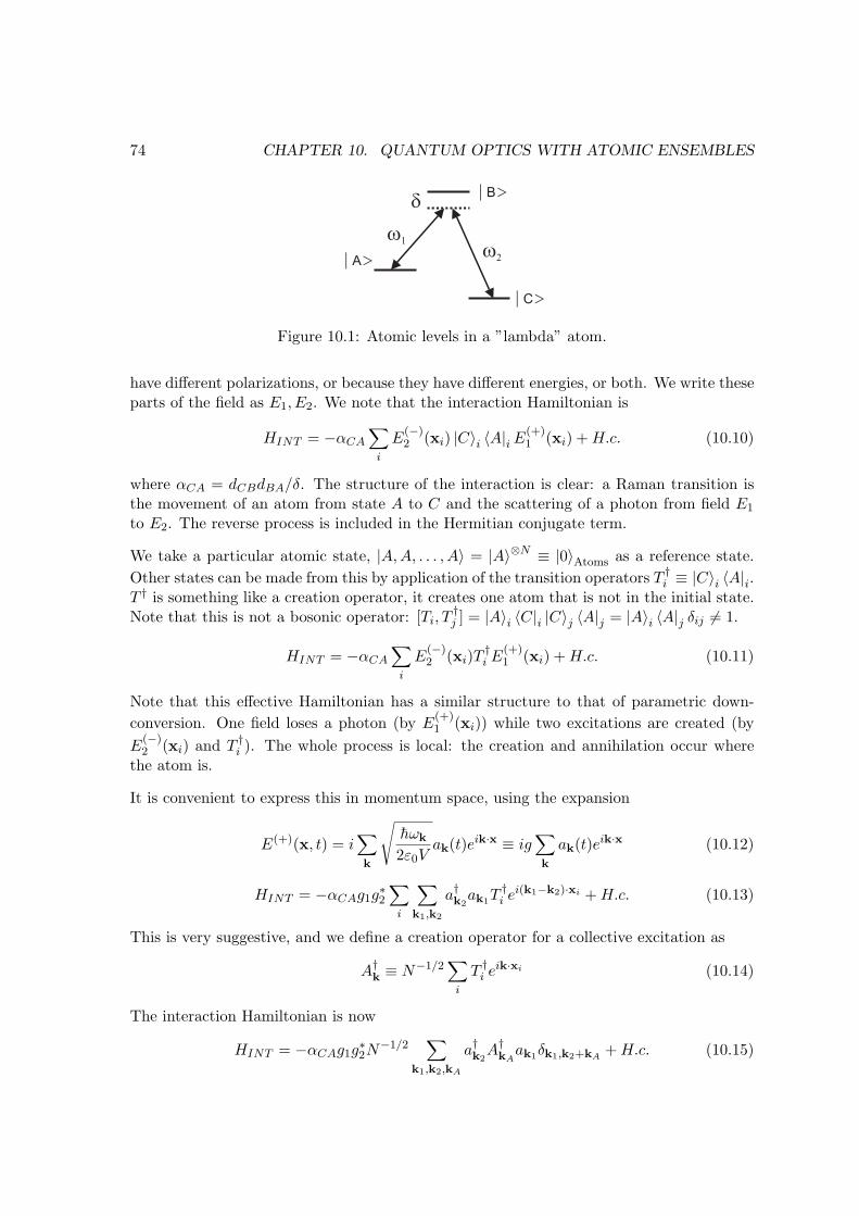
74 CHAPTER 10. QUANTUM OPTICS WITH ATOMIC ENSEMBLES
Figure 10.1: Atomic levels in a ”lambda” atom.
have different polarizations, or because they have different energies, or both. We write theseparts of the field as E1, E2. We note that the interaction Hamiltonian is
HINT = −αCA
∑
i
E(−)2 (xi) |C〉i 〈A|i E(+)
1 (xi) + H.c. (10.10)
where αCA = dCBdBA/δ. The structure of the interaction is clear: a Raman transition isthe movement of an atom from state A to C and the scattering of a photon from field E1
to E2. The reverse process is included in the Hermitian conjugate term.
We take a particular atomic state, |A,A, . . . , A〉 = |A〉⊗N ≡ |0〉Atoms as a reference state.Other states can be made from this by application of the transition operators T †i ≡ |C〉i 〈A|i.T † is something like a creation operator, it creates one atom that is not in the initial state.Note that this is not a bosonic operator: [Ti, T
†j ] = |A〉i 〈C|i |C〉j 〈A|j = |A〉i 〈A|j δij 6= 1.
HINT = −αCA
∑
i
E(−)2 (xi)T
†i E
(+)1 (xi) + H.c. (10.11)
Note that this effective Hamiltonian has a similar structure to that of parametric down-conversion. One field loses a photon (by E
(+)1 (xi)) while two excitations are created (by
E(−)2 (xi) and T †i ). The whole process is local: the creation and annihilation occur where
the atom is.
It is convenient to express this in momentum space, using the expansion
E(+)(x, t) = i∑
k
√hωk
2ε0Vak(t)eik·x ≡ ig
∑
k
ak(t)eik·x (10.12)
HINT = −αCAg1g∗2
∑
i
∑
k1,k2
a†k2ak1T
†i ei(k1−k2)·xi + H.c. (10.13)
This is very suggestive, and we define a creation operator for a collective excitation as
A†k ≡ N−1/2∑
i
T †i eik·xi (10.14)
The interaction Hamiltonian is now
HINT = −αCAg1g∗2N
−1/2∑
k1,k2,kA
a†k2A†kA
ak1δk1,k2+kA+ H.c. (10.15)
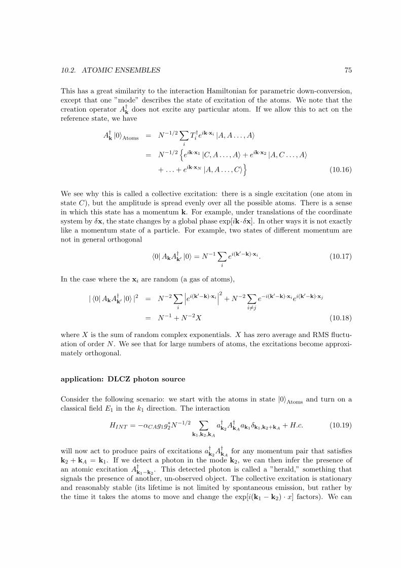
10.2. ATOMIC ENSEMBLES 75
This has a great similarity to the interaction Hamiltonian for parametric down-conversion,except that one ”mode” describes the state of excitation of the atoms. We note that thecreation operator A†k does not excite any particular atom. If we allow this to act on thereference state, we have
A†k |0〉Atoms = N−1/2∑
i
T †i eik·xi |A,A . . . , A〉
= N−1/2{eik·x1 |C,A . . . , A〉+ eik·x2 |A, C . . . , A〉
+ . . . + eik·xN |A,A . . . , C〉}
(10.16)
We see why this is called a collective excitation: there is a single excitation (one atom instate C), but the amplitude is spread evenly over all the possible atoms. There is a sensein which this state has a momentum k. For example, under translations of the coordinatesystem by δx, the state changes by a global phase exp[ik ·δx]. In other ways it is not exactlylike a momentum state of a particle. For example, two states of different momentum arenot in general orthogonal
〈0|AkA†k′ |0〉 = N−1∑
i
ei(k′−k)·xi . (10.17)
In the case where the xi are random (a gas of atoms),
| 〈0|AkA†k′ |0〉 |2 = N−2∑
i
∣∣∣ei(k′−k)·xi
∣∣∣2+ N−2
∑
i 6=j
e−i(k′−k)·xiei(k′−k)·xj
= N−1 + N−2X (10.18)
where X is the sum of random complex exponentials. X has zero average and RMS fluctu-ation of order N . We see that for large numbers of atoms, the excitations become approxi-mately orthogonal.
application: DLCZ photon source
Consider the following scenario: we start with the atoms in state |0〉Atoms and turn on aclassical field E1 in the k1 direction. The interaction
HINT = −αCAg1g∗2N
−1/2∑
k1,k2,kA
a†k2A†kA
ak1δk1,k2+kA+ H.c. (10.19)
will now act to produce pairs of excitations a†k2A†kA
for any momentum pair that satisfiesk2 + kA = k1. If we detect a photon in the mode k2, we can then infer the presence ofan atomic excitation A†k1−k2
. This detected photon is called a ”herald,” something thatsignals the presence of another, un-observed object. The collective excitation is stationaryand reasonably stable (its lifetime is not limited by spontaneous emission, but rather bythe time it takes the atoms to move and change the exp[i(k1 − k2) · x] factors). We can
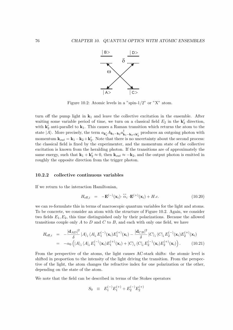
76 CHAPTER 10. QUANTUM OPTICS WITH ATOMIC ENSEMBLES
Figure 10.2: Atomic levels in a ”spin-1/2” or ”X” atom.
turn off the pump light in k1 and leave the collective excitation in the ensemble. Afterwaiting some variable period of time, we turn on a classical field E2 in the k′2 direction,with k′2 anti-parallel to k1. This causes a Raman transition which returns the atom to thestate |A〉. More precisely, the term ak′2Ak1−k2a
†k1−k2+k′2
produces an outgoing photon withmomentum kout = k1−k2+k′2. Note that there is no uncertainty about the second process:the classical field is fixed by the experimenter, and the momentum state of the collectiveexcitation is known from the heralding photon. If the transitions are of approximately thesame energy, such that k1 + k′2 ≈ 0, then kout ≈ −k2, and the output photon is emitted inroughly the opposite direction from the trigger photon.
10.2.2 collective continuous variables
If we return to the interaction Hamiltonian,
Heff,i = −E(−)(xi)· ↔αi ·E(+)(xi) + H.c. (10.20)
we can re-formulate this in terms of macroscopic quantum variables for the light and atoms.To be concrete, we consider an atom with the structure of Figure 10.2. Again, we considertwo fields E1, E2, this time distinguished only by their polarizations. Because the allowedtransitions couple only A to D and C to B, and each with only one field, we have
Heff,i = −|dAD|2δ
|A〉i 〈A|i E(−)1 (xi)E
(+)1 (xi)− |dCB|2
δ|C〉i 〈C|i E(−)
2 (xi)E(+)2 (xi)
= −α0
(|A〉i 〈A|i E(−)
1 (xi)E(+)1 (xi) + |C〉i 〈C|i E(−)
2 (xi)E(+)2 (xi)
). (10.21)
From the perspective of the atoms, the light causes AC-stark shifts: the atomic level isshifted in proportion to the intensity of the light driving the transition. From the perspec-tive of the light, the atom changes the refractive index for one polarization or the other,depending on the state of the atom.
We note that the field can be described in terms of the Stokes operators
S0 ≡ E(−)1 E
(+)1 + E
(−)2 E
(+)2
10.2. ATOMIC ENSEMBLES 77
Sx ≡ E(−)1 E
(+)2 + E
(−)2 E
(+)1
Sy ≡ i(E
(−)1 E
(+)2 − E
(−)2 E
(+)1
)
Sz ≡ E(−)1 E
(+)1 −E
(−)2 E
(+)2 (10.22)
Also, we can write ”spin” operators ji = (ji,x, ji,y, ji,z)T with
ji,0 =12
(|C〉i 〈C|i + |A〉i 〈A|i) =12
ji,x =12
(|A〉i 〈C|i + |C〉i 〈A|i)
ji,y =−i
2(|A〉i 〈C|i − |C〉i 〈A|i)
ji,z =12
(|C〉i 〈C|i − |A〉i 〈A|i) . (10.23)
These operators, whether or not they describe the true spin of the atom, behave like spin-1/2operators in that [jx, jy] = ijz/2 and cyclic permutations. We see that
Heff,i = −α0 (ji,0S0(xi) + ji,zSz(xi)) . (10.24)
If we assume that the field (or at least the Stokes operator Sz) does not change over theextent of the atoms, we can remove the dependence on xi. We can then sum to get
HINT = −α0 (J0S0 + JzSz) (10.25)
where J =∑
i ji describes a spin-N/2 system and obeys
[Ja, Jb] = iεabcJcN/2. (10.26)

78 CHAPTER 10. QUANTUM OPTICS WITH ATOMIC ENSEMBLES
Appendix A
Quantum theory for quantumoptics
This appendix describes some aspects of quantum theory that are either helpful, necessary,or simply illuminating, for the study of quantum optics.
A.1 States vs. Operators
The outcomes of measurements in quantum mechanics are described by expectation values.These could be average quantities such as 〈x〉 , ⟨x2
⟩, etc. or they could be frequencies of
particular outcomes, which are described as the expectation values of a projector. Forexample a projector onto the state |φ〉 is Pφ = |φ〉 〈φ|, so that the probability of finding asystem in state |φ〉 is 〈Pφ〉. This holds also for continuous-valued probability distributions,such as |ψ(x)|2, which can be found as the expectation values of projectors onto small (inthe limit infinitessimal), regions around x.
An expectation value 〈φ|A |φ〉 will evolve as
〈A〉φ (t) = 〈φ|U †(t)AU(t) |φ〉= 〈φ(t)|S A |φ(t)〉S= 〈φ|AH(t) |φ〉 (A.1)
where U(t) is the time-evolution operator, and |φ(t)〉S = U(t) |φ〉 and AH(t) = U †(t)AU(t)are the Schrodinger picture state and Heisenberg picture operator, respectively. Thesepictures are completely equivalent in their results, and in some sense, the difference betweenthem is trivial; what we really want to know is the time evolution U(t). At the same time,the Schrodinger picture is more familiar to most people (it is usually taught first). So whyis quantum optics always described in the Heisenberg picture?
One good reason is the classical-quantum correspondence. The equations for the quantum
79
80 APPENDIX A. QUANTUM THEORY FOR QUANTUM OPTICS
field operators are exactly the same as the equations for the corresponding classical fields,with the consequence that the average values of the two theories will agree. Another goodreason is that many problems in field theory are very high-dimensional, so that a fulldescription of the state would be very complicated. In contrast, a description of the fewoperators that we will eventually measure may be much simpler. Finally, there are a fewcentral problems where operators are easy to work with, and states very difficult. One ofthese is the beam-splitter, described in an earlier chapter.
A.2 Calculating with operators
A.2.1 Heisenberg equation of motion
Given a Hamiltonian H(t), and an arbitrary operator A, the evolution of A is given by
d
dtA =
1ih
[A,H(t)] + ∂tA (A.2)
where ∂tA is the explicit time-dependence of A. For example, if B = q exp[iωt] where q issome operator which itself will change in time due to the Hamiltonian, then
d
dtB =
1ih
[q,H(t)] exp[iωt] + iωq exp[iωt]. (A.3)
Typically we will avoid operators with explicit time dependence.
A.2.2 Time-dependent perturbation theory
A very useful form of perturbation theory was developed by F. Dyson, based on the inter-action picture. The unitary time-evolution operator U(t) obeys the Schrodinger equation1
id
dtU(t) = H(t)U(t) (A.4)
with the initial condition U(0) = I. When the Hamiltonian is broken into two parts as
H = H0 + H ′, (A.5)
it is convenient to also divide U asU = U0UI (A.6)
where U0 is the unperturbed evolution, i.e., idU0/dt = H0U0 so that
id
dt(U0UI) = (H0 + H ′)U0UI
1Note that we are dropping the factors of h here. They are easy to put back, just by noting that the Hand h always occur together in the combination H/h.
A.2. CALCULATING WITH OPERATORS 81
i(d
dtU0)UI + iU0(
d
dtUI) = H0U0UI + H ′U0UI
id
dtUI = U †
0H ′U0UI
≡ HIUI . (A.7)
The operator HI is the interaction picture Hamiltonian, and the evolution UI describesthe change in the state, relative to the state evolution under H0 alone. For example,⟨U †
0(t)U(t)⟩
φ= 〈U0(−t)U0(t)UI(t)〉φ = 〈UI(t)〉φ is the overlap of the state |φ〉, evolved
under H, with the same state evolved under just H0.
It is easy to check that the evolution of UI ,
id
dtUI = HIUI (A.8)
is solved by
UI(t) =
[1− i
∫ t
0dt′HI(t′)−
∫ t
0dt′
∫ t′
0dt′′HI(t′)HI(t′′) + . . .
]
= T e−i∫ t
0dt′HI(t′). (A.9)
This expansion is known as the Dyson series. Note that the integrals contain the time-ordered products HI(t′)HI(t′′)HI(t′′′) . . . with t′ > t′′ > t′′′ > . . . The symbol T indicatestime-ordering, so that the exponential agrees with the expansion in the line above it. It isalso convenient to know U †
I
U †I (t) =
[1 + i
∫ t
0dt′HI(t′)−
∫ t
0dt′
∫ t′
0dt′′HI(t′′)HI(t′) + . . .
]
= T e+i∫ t
0dt′HI(t′). (A.10)
Note that here the operators are anti-time-ordered (T ).
Using these results, in the Schrodinger picture, states evolve as
|ψ(t)〉 = U0(t)T e−i∫ t
0dt′HI(t′) |ψ(t = 0)〉 (A.11)
while in the Heisenberg picture operators evolve as
A(t) = T e+i∫ t
0dt′HI(t′)U †
0(t)A(0)U0(t)T e−i∫ t
0dt′HI(t′)
= T e+i∫ t
0dt′HI(t′)A0(t)T e−i
∫ t
0dt′HI(t′) (A.12)
where A0(t) ≡ U †0(t)A(0)U0(t) is the unperturbed evolution of the operator A, i.e., the
evolution under only H0 from the initial value A(0). Expanding the first few terms
A(t) = A0(t)
82 APPENDIX A. QUANTUM THEORY FOR QUANTUM OPTICS
+i
∫ t
0dt′HI(t′)A0(t)− iA0(t)
∫ t
0dt′HI(t′)
−∫ t
0dt′
∫ t′
0dt′′HI(t′′)HI(t′)A0(t)
−A0(t)∫ t
0dt′
∫ t′
0dt′′HI(t′)HI(t′′)
+∫ t
0dt′HI(t′)A0(t)
∫ t
0dt′HI(t′)
+O(H3I ) (A.13)
It is interesting also to take the time derivative of this equation to get the rate of change ofA
d
dtA(t) =
d
dtA0(t)− i[A0(t),HI(t)]
−∫ t
0dt′
[[A0(t), HI(t′)
],HI(t)
]+ O(H3
I ) (A.14)
A.2.3 example: excitation of atoms to second order
We assume a collection of very simple atoms, labeled by the index i, with ground andexcited states |g〉i and |e〉i, respectively and transition frequencies ωi. For simplicity, weassume the atoms are all in the same place. We define bi ≡ |g〉i 〈e|i and b†i ≡ |e〉i 〈g|i forconvenience. If the ground state has zero energy, the Hamiltonian is
H = HEM +∑
i
hωib†ibi + gE(+)b†i + g∗E(−)bi. (A.15)
An explanation of this Hamiltonian is given in Chapter ??. For the moment, just note thatthe last two terms are reasonable; one term excites an atom while destroying a photon, andthe other accomplishes the reverse process. We identify the first two terms as H0 and thelast two as H ′. Under H0 (specifically the part HEM ), the field E evolves as E0(t), theevolution under Maxwell’s equations from whatever is the initial condition. Under H0 theatomic operator bi evolves as b0,i(t) = bi(0) exp[−iωit]. The interaction Hamiltonian is thus
HI =∑
i
gE(+)0 (t)b†i (0)eiωit + g∗E(−)
0 (t)bi(0)e−iωit. (A.16)
We calculate the evolution of ni as follows: First, [n0,i,H0(t)] = 0, so n0,i(t) is a constant.Also,
[n0,i,HI(t)] = gE(+)0 (t)b†i (0)eiωit − g∗E(−)
0 (t)bi(0)e−iωit (A.17)
and[[
n0,i,HI(t′)],HI(t)
]= |g|2
[n0,iE
(+)0 (t′)E(−)
0 (t)e−iωi(t−t′)
−(1− n0,i)E(−)0 (t)E(+)
0 (t′)e−iωi(t−t′)
A.2. CALCULATING WITH OPERATORS 83
−(1− n0,i)E(−)0 (t′)E(+)
0 (t)eiωi(t−t′)
+ n0,iE(+)0 (t)E(−)
0 (t′)eiωi(t−t′)]
(A.18)
As a result, the rate of change of ni is
d
dtni(t) = −igE
(+)0 (t)b†i (0)eiωit + ig∗E(−)
0 (t)bi(0)e−iωit
−|g|2∫ t
0dt′
[n0,iE
(+)0 (t′)E(−)
0 (t)e−iωi(t−t′)
−(1− n0,i)E(−)0 (t)E(+)
0 (t′)e−iωi(t−t′)
−(1− n0,i)E(−)0 (t′)E(+)
0 (t)eiωi(t−t′)
+ n0,iE(+)0 (t)E(−)
0 (t′)eiωi(t−t′)]
+O(H3I ). (A.19)
The first line indicates the conversion of coherence between atomic levels 〈b〉 ,⟨b†
⟩, to
population. The next two lines describe second-order processes. Note that the product(1−n0,i)E
(−)0 E
(+)0 is, very roughly speaking, the probability to find the atom in the ground
state times the intensity, indicating that the presence of photons can (in second order) causethe transition g → e. The product n0,iE
(+)0 E
(−)0 is, again roughly speaking, the probability
to find the atom in the excited state times (intensity + vacuum fluctuations). This termproduces both spontaneous and stimulated emission e → g.
If an atom starts in its ground state, we have 〈b0,i〉 =⟨b†0,i
⟩= 〈n0,i〉 = 0, so that
d
dt〈ni(t)〉 =
|g|2h2
∫ t
0dt′
⟨E
(−)0 (t)E(+)
0 (t′)e−iωi(t−t′) + E(−)0 (t′)E(+)
0 (t)eiωi(t−t′)⟩
(A.20)
where we have dropped the higher-order terms. A rough interpretation would be: the rateof excitation is the current field E
(−)0 (t) times the accumulation of field at the transition
frequency exp[−iωit]∫ t0 dt′E(+)
0 (t′) exp[iωit′].
A.2.4 Glauber’s broadband detector
Glauber based his celebrated theory of photo-detection on exactly the problem of a collectionof atoms excited by a quantum field. Assume the transition frequencies ωi are distributedover a broad range by some unspecified mechanism of inhomogeneous broadening, so thatthe detector has a broad bandwidth. Assuming that the detector has some mechanismwhich produces an electrical output signal in response to excited atoms, we calculate therate of change of the operator
Ne ≡∑
i
ni (A.21)
84 APPENDIX A. QUANTUM THEORY FOR QUANTUM OPTICS
which is the total number of excitations. Assuming as above that each atom starts in itsground state, the average rate of detections (increase in number of excited atoms) is
d
dt〈N(t)〉 =
|g|2h2
∑
i
∫ t
0dt′
⟨E
(−)0 (t)E(+)
0 (t′)e−iωi(t−t′) + E(−)0 (t′)E(+)
0 (t)eiωi(t−t′)⟩
. (A.22)
Assuming there are many atoms, the sum can be replaced by an integral∑
i →∫
dωiρ(ωi)where ρ is a ”density of states” factor. Assuming that ρ(ω) = ρ is flat, i.e., broad-band, theintegral
∫dωiρ(ωi) exp[−iωi(t− t′)] = 2πρδ(t− t′) and the integral over t′ can be evaluated
simply. We thus arrive to Glauber’s result
d
dt〈N(t)〉 = 2πρ
|g|2h2
⟨E
(−)0 (t)E(+)
0 (t)⟩
. (A.23)
Note that E(−)0 (t)E(+)
0 (t) in the RHS is normally-ordered. This implies that in the absenceof photons, there will be no detections. This obviously agrees with our experience of photo-detection, and resolves a basic question: why don’t photo-detectors (or our eyes!) see thevacuum fluctuations? While there is energy in the vacuum,
⟨E2
⟩ 6= 0, detectors do notrespond to energy, but rather to photons.
A.3 Second quantization
In Chapter 2, we used canonical quantization to find a quantum theory of the electro-magnetic field. This theory describes the evolution of field operators, which can be ex-pressed in terms of creation and annihilation operators for field modes, and these behavelike quantum mechanical harmonic oscillators. In this description, a photon is an excitationof a harmonic oscillator.
This theory may not seem to have much in common with the quantum mechanics of otherparticle such as electrons or atoms, but it does. We can describe other bosonic particles in avery similar, field-theoretic way. This gives a lot of insight into what is going on with light.This is the subject of second quantization, the description of collections of particles usingfield operators. The name ”second quantization” is a bit misleading. In the quantization ofthe EM field, we invented a new quantum theory based on an old, classical theory. In secondquantization there is no new theory, it is simply a way to write an old theory (quantummechanics) using field-theoretic notation. When we are done, quantum mechanics will lookjust like quantum optics.
Collections of bosonic particles, such as photons, 4He, and most of the atoms that can belaser cooled, are described by exchange-symmetric wave-functions. For the moment, wework with time-independent wave-functions. Later we will consider how the states evolve.If we write two orthonormal single-particle wave-functions as φ1(x), φ2(x), then possibletwo-particle wave-functions are
Ψφ1φ2(x1, x2) =1√2
[φ1(x1)φ2(x2) + φ1(x2)φ2(x1)]
A.3. SECOND QUANTIZATION 85
Ψφ21(x1, x2) =
12
[φ1(x1)φ1(x2) + φ1(x2)φ1(x1)] = φ1(x1)φ1(x2). (A.24)
We note that both are symmetric under the exchange x1 ↔ x2. Because of the exchangesymmetry requirement, Ψ is completely determined by the wave-functions φ1(x), φ2(x),and by how many particles occupy each single-particle state. For this reason, we can usethe labels φ1φ2 and φ2
1 to describe these two states, where the superscript indicates theoccupancy.
A general N-particle bosonic state is described by
Ψφn11 φ
n22 ...(x1, x2 . . .) ≡ 1√
N !n1!n2! . . .
∑
P{x1,x2,...,xN}
n1︷ ︸︸ ︷φ1(x1)φ1(x2) . . . φ1(xn1)
n2︷ ︸︸ ︷φ2(xn1+1) . . .
(A.25)where the sum is over all possible permutations of {x1, x2, . . . , xN} and the factor underthe square root is needed to preserve normalization. We will write the state which has thiswave function as |φn1
1 φn22 . . .〉.
If our goal were to treat a system with a fixed number of particles, we could work with thewave-function above, for example write down the Schrodinger equation that it obeys, tryto find solutions, etc. But there are many situations where the number of particles is notfixed. Examples include reactions such as γ → e−+e+ in high energy physics, or absorptionof photons by material, which in a semiconductor might produce the reaction γ → e− + h+
where h+ indicates a ”hole,” a positive charge carrier. If we want to think about thesesituations, we need to be able to describe states with variable numbers of photons. Forexample, we could write a state
|Σ〉 = c0 |0〉+ c1 |φa〉+ c2 |φbφc〉+ . . . (A.26)
where the c1 term describes the part of the state with one particle, the c2 part describesthe part of the state with two particles, etc. The c0 part of the state is something new,and clearly necessary if particles can be destroyed. It describes the amplitude for havingno particles, which we call ”vacuum” and write as |0〉.We also see that now we can describe operators which change the number of particles, forexample |φ2〉 〈φ1φ2| is a valid operator. It converts the state |φ1φ2〉 into the state |φ2〉 (andannihilates anything else). This operator would only have a nonzero expectation value ifthe state contained both |φ1φ2〉 and |φ2〉, i.e., if the state had an indeterminate number ofparticles. We can define aφi , the annihilation operator for the state φi through
aφi |φn11 φn2
2 . . . φnii . . .〉 =
√ni
∣∣∣φn11 φn2
2 . . . φni−1i . . .
⟩. (A.27)
This describes the removal of a particle from the single-particle state φi. The factor√
ni
will be the subject of a problem. The creation operator a†φifor the same state acts as
a†φi|φn1
1 φn22 . . . φni
i . . .〉 =√
ni + 1∣∣∣φn1
1 φn22 . . . φni+1
i . . .⟩
. (A.28)
86 APPENDIX A. QUANTUM THEORY FOR QUANTUM OPTICS
It is easy to check that
|φn11 φn2
2 . . .〉 =
(a†φ1
)n1
√n1!
(a†φ2)n2
√n2!
. . .
|0〉 (A.29)
and that the creation and annihilation operators obey
[aφi , aφj ] = [a†φi, a†φj
] = 0
[aφi , a†φj
] = δij . (A.30)
Clearly there is a similarity between these operators and the creation and annihilationoperators for the modes of the electromagnetic field.
Field operators
The crucial step in second quantization (some might say the only step) is the introductionof field operators. We consider the case where the φi(x) are the single-particle energyeigenstates with energies hωi. A single particle wave-function evolves as
φi(x, t) = e−iωitφi(x, 0). (A.31)
We also assume for simplicity that the particles are non-interacting, so that the evolutionof a multi-particle wave function is
φ1(x, t)φ2(x, t) . . . = e−iω1tφ1(x, 0)e−iω2tφ2(x, 0) . . . (A.32)
We define the field operator Φ(x, t) as
Φ(x, t) ≡∑
i
aφiφi(x, t) =∑
i
aφiφi(x, 0)e−iωit (A.33)
with Hermitian conjugate
Φ†(x, t) ≡∑
i
a†φiφ∗i (x, t) =
∑
i
a†φiφ∗i (x, 0)eiωit. (A.34)
These field operators are very powerful, and have a simple interpretation. Consider thestate Φ†(x, 0) |0〉, which clearly contains only one particle. The state is
|ψ〉 =∑
i
φ∗i (x, 0) |φi〉 (A.35)
with wave-functionΨ(x1) =
∑
i
φ∗i (x, 0)φi(x1, 0) = δ(x1 − x) (A.36)
by completeness of the states φ. From this we see that Φ†(x) creates a particle at positionx. Similarly, Φ(x) destroys a particle at position x.
A.3. SECOND QUANTIZATION 87
We note that Φ and Φ† are very similar to the positive and negative frequency parts of thequantized electric field E(+) and E(−) defined in Chapter 4.
E(+)(r, t) = i∑
k,α
√hωk
2ε0ak,αuk,α(r)e−iωkt
E(−)(r, t) = −i∑
k,α
√hωk
2ε0ak,αu∗k,α(r)eiωkt (A.37)
At this point, we have turned ordinary quantum mechanics of many bosons into a fieldtheory. Perhaps surprisingly, the same can be done for fermions, which have exchange anti-symmetric wave functions and thus obey the Pauli exclusion principle. The only changethat is necessary is to replace the creation and annihilation operators a and a† for creationand annihilation operators b and b† which obey the anti-commutation relation {bi, b
†j} = δij .
You might ask, why would we want ordinary quantum mechanics to look like field the-ory? Because the tools of field theory can be applied very easily to situations with variablenumbers of particles. Examples would be systems in contact with a reservoir, thermal pro-duction of particles such as phonons, and Bose-Einstein condensation. The field operatorsoften behave something like system-wide versions of a single-particle wave function. Forexample,
∫dxΦ†(x)Φ(x) =
∫dx
∑
ij
φ∗i (x)φj(x)a†φiaφj =
∑
i
a†φiaφi =
∑
i
ni, (A.38)
where the middle step follows from the orthonormality of the states φ. Since the lastexpression is the total number of particles, we conclude that Φ†(x)Φ(x) is a sort of particle-density operator. Also, any single-particle operator A, with matrix elements
Aij ≡ 〈φi|A |φj〉 =∫
dxφ∗i (x)Aφj(x) (A.39)
will have a multi-particle equivalent. Explicitly,∫
dxΦ†(x)AΦ(x) =∫
dx∑
ij
φ∗i (x)Aφj(x)a†φiaφj =
∑
ij
a†φiAijaφj . (A.40)
This describes, in a very natural way, the total value of A, including the contributions ofall particles. Similarly, a two-particle interaction potential V (x, x′) can be applied to thewhole collection of particles with an operator 1/2
∫dx dx′Φ†(x)Φ†(x′)V (x, x′)Φ†(x′)Φ†(x).
88 APPENDIX A. QUANTUM THEORY FOR QUANTUM OPTICS
Related Documents