Quantum mechanics of many-particle systems - Learning

Basic Books in Science

Book 12

Quantum Mechanics of

Many-Particle Systems:

Atoms, Molecules – and More

Roy McWeeny

BASIC BOOKS IN SCIENCE

– a Series of books that start at the beginning

Book 12 Draft Version (10 May 2014) of all Chapters

Quantum mechanics of many-particlesystems: atoms, molecules – and more

Roy McWeeny

Professore Emerito di Chimica Teorica, Universita di Pisa, Pisa (Italy)

The Series is maintained, with regular updating and improvement, at

http://www.learndev.org/ScienceWorkBooks.html

and the books may be downloaded entirely free of charge.

This book is licensed under a Creative CommonsAttribution-ShareAlike 3.0 Unported License.

:

(Last updated 10 May 2014)

BASIC BOOKS IN SCIENCE

Acknowledgements

In a world increasingly driven by information technology no educational experiment canhope to make a significant impact without effective bridges to the ‘user community’ – thestudents and their teachers.

In the case of “Basic Books in Science” (for brevity, “the Series”), these bridges have beenprovided as a result of the enthusiasm and good will of Dr. David Peat (The Pari Centerfor New Learning), who first offered to host the Series on his website, and of Dr. JanVisser (The Learning Development Institute), who set up a parallel channel for furtherdevelopment of the project. The credit for setting up and maintaining the bridgeheads,and for promoting the project in general, must go entirely to them.

Education is a global enterprise with no boundaries and, as such, is sure to meet linguisticdifficulties: these will be reduced by providing translations into some of the world’s mostwidely used languages. Dr. Angel S. Sanz (Madrid) is preparing Spanish versions of thebooks and his initiative is most warmly appreciated. In 2014 it is our hope that translatorswill be found for French and Arabic versions.

We appreciate the interest shown by universities in Sub-Saharan Africa (e.g. Universityof the Western Cape and Kenyatta University), where trainee teachers are making useof the Series; and that shown by the Illinois Mathematics and Science Academy (IMSA)where material from the Series is being used in teaching groups of refugee children frommany parts of the world.

All who have contributed to the Series in any way are warmly thanked: they have givenfreely of their time and energy ‘for the love of Science’.

Pisa, 10 May 2014 Roy McWeeny (Series Editor)

i

BASIC BOOKS IN SCIENCE

About this book

This book, like the others in the Series1, is written in simple English – the language mostwidely used in science and technology. It builds on the foundations laid in earlier Books,which have covered many areas of Mathematics and Physics.

The present book continues the story from Book 11, which laid the foundations of Quan-tum Mechanics and showed how it could account succesfully for the motion of a singleparticle in a given potential field. The almost perfect agreement between theory andexperiment, at least for one electron moving in the field of a fixed positive charge, seemedto confirm that the principles were valid – to a high degree of accuracy. But what if wewant to apply them to much more complicated systems, such as many-electron atomsand molecules, in order to get a general understanding of the structure and properties ofmatter? At first sight, remembering the mathematical difficulty of dealing with a single

electron in the Hydrogen atom, we seem to be faced with an impossible task. The aim ofBook 12 is to show how, guided by the work of the pioneers in the field, an astonishingamount of progress can be made. As in earlier books of the Series, the path to be followedwill avoid a great deal of unnecessary detail (much of it being only of historical interest)in order to expose the logical development of the subject.

1The aims of the Series are described elsewhere, e.g. in Book 1.

ii

Looking ahead –

In Book 4, when you started on Physics, we said “Physics is a big subject and you’ll needmore than one book”. Here is another one! Book 4 was mainly about particles, theways they move when forces act on them, and how the same ‘laws of motion’ still holdgood for all objects built up from particles – however big they may be. In Book 11 wemoved from Classical Physics to Quantum Physics and again started with the study ofa single moving particle and the laws that govern its behaviour. Now, in Book 12, wemove on and begin to build up the ‘mathematical machinery’ for dealing with systemscomposed of very many particles – for example atoms, where up to about 100 electronsmove in the electric field of one nucleus, or molecules, where the electrons move in thefield provided by several nuclei.

• Chapter 1 reviews the priciples formulated in Book 11, along with the conceptsof vector space, in which a state vector is associated with the state of motion ofa particle, and in which an operator may be used to define a change of state. Thischapter uses Schrodinger’s form of quantum mechanics in which the state vectorsare ‘represented’ by wave functions Ψ = Ψ(x, y, z) (functions of the position of theparticle in space) and the operators are typically differential operators. The chapterstarts from the ideas of ‘observables and measurement’; and shows how mea-surement of a physical quantity can be described in terms of operations in a vectorspace. It follows with a brief reminder of the main way of calculating approximatewave functions, first for one electron, and then for more general systems.

• In Chapter 2 you take the first step by going from one electron to two: theHamiltonian operator is then H(1, 2) = h(1) + h(2) + g(1, 2), where only g – the‘interaction operator’ – depends on the coordinates of both particles. With neglectof interaction the wave function can be taken as a product Psi(1, 2) = ψa(1)ψb(2),which indicates Particle 1 in state ψa and Particle 2 in state ψb. This is a firstexample of the Independent Particle Model and can give an approximate wavefunction for a 2-particle system. The calculation of the ground state electronicenergy of the Helium atom is completed with an approximate wave function ofproduct form (two electrons in an orbital of 1s type) and followed by a study of theexcited states that result when one electron is ‘promoted’ into the 2s orbital. Thisraises interesting problems about the symmetry of the wave function. There are, itseems, two series of possible states: in one the function is unchanged if you swap theelectrons (it is symmetric) but in the other it changes in sign (it is antisymmetric).Which must we choose for two electrons?

At this point we note that electron spin has not yet been taken into account.The rest of the chapter brings in the spin functions α(s) and β(s) to describe anelectron in an ‘up-spin’ or a ‘down-spin’ state. When these spin factors are includedin the wave functions an orbital φ(r) (r standing for the three spatial variables

iii

x, y, z) is replaced by a spin-orbital ψ(r, s) = φ(r)α(s) (for an up-spin state) orψ(r, s) = φ(r)β(s) (for a down-spin state).

The Helium ground state is then found to be

Ψ(x1,x2) = φ(r1)φ(r2)[α(s1)β(s2)− α(s1)β(s2)],

where, from now on, a boldface letter (x) will denote ‘space-and-spin’ variables.Interchanging Electron 1 and Electron 2 then shows that only totally antisymmetric

wavefunctions can correctly predict the observed properties of the system. Moregenerally, this is accepted as a fundamental property of electronic systems.

• Chapter 3 starts from the Antisymmetry Principle and shows how it can beincluded generally in the Independent Particle Model for an N -electron system.Slater’s rules are derived as a basis for calculating the total energy of such a sys-tem in its ‘ground state’, where only the lowest-energy spin-orbitals are occupiedby electrons. In this case, neglecting tiny spin-dependent effects, expressions forthe ground-state energies of the first few many-electron atoms (He, Li, Be, ...) areeasily derived.

• So far, we have not considered the analytical forms of the orbitals themselves,assuming that the atomic orbitals (AOs) for a 1-electron system (obtained in Book11) will give a reasonable first approximation. In actual fact that is not so andthe whole of this difficult Chapter 4 is devoted to the Hartree-Fock method ofoptimizing orbital forms in order to admit the effects of inter-electron repulsion.By defining two new one-electron operators, the Coulomb operator J and theExchange operator K, it is possible to set up an effective 1-electron HamiltonianF (the ‘Fock operator’) whose eigenfunctions will be ‘best possible approximations’to the orbitals in an IPM wave function; and whose corresponding eigenvalues givea fairly realistic picture of the distribution of the total electronic energy E amongthe individual electrons. In fact, the eigenvalue ǫk represents the amount of energy‘belonging to’ an electron in orbital φk; and this can be measured experimentally byobserving how much energy is needed to knock the electron out. This gives a firmbasis for the much-used energy-level diagrams. The rest of Chapter 4 deals withpractical details, showing how the Hartree-Fock equation Fφ = ǫφ can be written(by expanding φ in terms of a set of known functions) in the finite basis form

Fc = ǫc, where F is a square matrix representing the Fock operator and c is acolumn of expansion coefficients.

• At last, in Chapter 5, we come to the first of the main themes of Book 12: “Atoms– the building blocks of matter”. In all atoms, the electrons move in the field of acentral nuclus, of charge Ze, and the spherical symmetry of the field allows us touse the theory of angular momentum (Chapter 5 of Book 11) in classifying thepossible stationary states. By assigning the Z electrons to the 1-electron states (i.e.orbitals) of lowest energy we obtain the electron configuration of the electronic

iv

ground state; and by coupling the orbital angular momentum of individual electrons,in s, p, d, ... states with quantum numbers l = 0, 1, 2, ... it is possible to setup many-electron states with quantum numbers L = 0, 1, 2, ... These are calledS, P, D, ... states and correspond to total angular momentum of 0, 1, 2, ... units:a state of given L is always degenerate, with 2L+1 component states in which theangular momentum component (along a fixed z-axis) goes down in unit steps fromM = L to M = −L. Finally, the spin angular momentum must be included.

The next step is to calculate the total electronic energy of the various many-electronstates in IPM approximation, using Slater’s Rules. All this is done in detail, usingworked examples, for the Carbon atom (Section 5.2). Once you have found wavefunctions for the stationary states, in which the expectation values of observablesdo not change in time, you’ll want to know how to make an atom jump from onestate to another. Remember from Book 10 that radiation consists of a rapidlyvarying electromagnetic field, carried by photons of energy ǫ = hν, where h isPlanck’s constant and νis the radiation frequency. When radiation falls on anatom it produces a small oscillating ‘perturbation’ and if you add this to the free-atom Hamiltonian you can show that it may produce transitions between statesof different energy. When this energy difference matches the photon energy hν aphoton will be absorbed by, or emitted from, the atom. And that is the basis ofall kinds of spectroscopy – the main experimental ‘tool’ for investigating atomicstructure.

The main theoretical tool for visualizing what goes on in atoms and molecules isprovided by certain electron density functions, which give a ‘classical’ picture ofhow the electric charge, or the electron spin, is ‘spread out’ in space. These densities,which you first met in Chapter 4, are essentially components of the density matrix.The properties of atoms, as atomic number (i.e. nuclear charge, Z) increases, areusually displayed in a Periodic Table, which makes a clear connection betweenelectronic and chemical properties of the elements. Here you find a brief descriptionof the distribution of electrons among the AOs of the first 36 atoms.

This chapter ends with a brief look at the effects of small terms in the Hamiltonian,so far neglected, which arise from the magnetic dipoles associated with electronspins. The electronic states discussed so far are eignstates of the Hamiltonian H,the total angular momentum (squared) L2, and one component Lz. But when spinis included we must also admit the total spin with operators S2 and Sz, formed bycoupling individual spins; the total angular momentum will then have componentswith operators Jx = Lx + Sx etc. The magnetic interactions between orbital andspin dipoles then lead to the fine structure of the energy levels found so far. Theexperimentally observed fine structure is fairly well accounted for, even with IPMwave functions.

• Atoms first started coming together, to form the simplest molecules, in the veryearly Universe. In Chapter 6 “Molecules: the first steps – ” you go back to the

v

‘Big Bang’, when all the particles in the present Universe were contained in a small‘ball’ which exploded – the interactions between them driving them apart to formthe Expanding Universe we still have around us today. The first part of thechapter tells the story, as best we know it, from the time when there was nothingbut an unbelievably hot ‘sea’ (nowadays called a plasma) of electrons, neutrons andprotons, which began to come together in Hydrogen atoms (1 proton + 1 electron).Then, when another proton is added, you get a hydrogen molecule ion H +

2 – andso it goes on!

In Section 6.2 you do a simple quantum mechanical calculation on H +2 , combining

two hydrogen-like atomic orbitals to form two approximate eigenfunctions for oneelectron in the field of two stationary protons. This is your first molecular orbital(MO) calculation, using ‘linear combination of atomic orbitals’ to obtain LCAOapproximations to the first two MOs: the lower energy MO is a Bonding Orbital,the higher energy MO is Antibonding.

The next two sections deal with the interpretation of the chemical bond – where doesit come from? There are two related interpretations and both can be generalized atonce to the case of many-electon molecules. The first is based on an approximatecalculation of the total electronic energy, which is strongly negative (describing theattraction of the electrons to the positive nuclei): this is balanced at a certaindistance by the positive repulsive energy between the nuclei. When the total energyreaches a minimum value for some configuration of the nuclei we say the system isbonded. The second interpretation arises from an analysis of the forces acting onthe nuclei: these can be calculated by calculating the energy change when a nucleusis displaced through an infinitesimal distance. The ‘force-concept’ interpretation isattractive because it gives a clear physical picture in terms of the electron density

function: if the density is high between two nuclei it will exert forces bringing themtogether.

• Chapter 7 begins a systematic study of some important molecules formed mainlyfrom the first 10 elements in the Periodic Table, using the Molecular Orbital ap-proach which comes naturally out of the SCF method for calculating electronic wavefunctions. This may seem to be a very limited choice of topics but in reality it in-cludes a vast range of molecules: think of the Oxygen (O2) in the air we breath, thewater (H2O) in our oceans, the countless compounds of Hydrogen, Carbon, Oxygenthat are present in all forms of plant and animal life.

In Section 7.1 we begin the study of some simple diatomic molecules such as Lithiumhydride (LiH) and Carbon monoxide (CO), introducing the idea of ‘hybridization’in which AOs with the same principal quantum number are allowed to mix in usingthe variation method. Another key concept in understanding molecular electronicstructure is that of the Correlation Diagram, developed in Section 7.2, whichrelates energy levels of the MOs in a molecule to those of the AOs of its constituentatoms. Figures 7.2 to 7.5 show simple examples for some diatomic molecules. The

vi

AO energy levels you know something about already: the order of the MO levelsdepends on simple qualitative ideas about how the AOs overlap – which dependsin turn on their sizes and shapes. So even without doing a big SCF calculation itis often possible to make progress using only pictorial arguments. Once you havean idea of the probable order of the MO energies, you can start filling them withthe available valence electrons and when you’ve done that you can think about theresultant electron density! Very often a full SCF calculation serves only to confirmwhat you have already guessed.

In Section 7.3 we turn to some simple polyatomic molecules, extending the ideasused in dealing with diatomics to molecules whose experimentally known shapessuggest where localized bonds are likely to be found. Here the most importantconcept is that of hybridization – the mixing of s and p orbitals on the same centre,to produce hybrids that can point in any direction. It soon turns out that hybrids ofgiven form can appear in sets of two, three, or four; and these are commonly foundin linear molecules, trigonal molecules (three bonds in a plane, at 120◦ to eachother) and tetrahedral molecules (four bonds pointing to the corners of a regulartetrahedron). Some systems of roughly tetrahdral form are shown in Figure 7.7.

It seems amazing that polyatomic molecules can often be well represented in termsof localized MOs similar to those found in diatomics. In Section 7.4 this mystery isresolved in a rigorous way by showing that the non-localized MOs that arise from ageneral SCF calculation can be mixed by making a unitary transformation – withoutchanging the form of the total electron density in any way! This is another exampleof the fact that only the density itself (e.g. |ψ|2, not ψ) can have a physical meaning.

Section 7.5 turns towards bigger molecules, particularly those important for OrganicChemistry and the Life Sciences, with fully worked examples. Many big molecules,often built largely from Carbon atoms, have properties connected with loosely boundelectrons occupying π-type MOs that extend over the whole system.

Such molecules were a favourite target for calculations in the early days of QuantumChemistry (before the ‘computer age’) because the π electrons could be consideredby themselves, moving in the field of a ‘framework’, and the results could easilybe compared with experiment. Many molecules of this kind belong to the classof alternant systems and show certain general properties. They are considered inSection 7.6, along with first attempts to discuss chemical reactivity.

To end this long chapter, Section 7.7 summarizes and extends the ‘bridges’ estab-lished between Theory and Experiment, emphasizing the pictorial value of densityfunctions such as the electron density, the spin density, the current density and soon.

• Chapter 8 Extended Systems: Polymers, Crystals and New Materials

concludes Book 12 with a study of applications to systems of great current inter-est and importance, for the Life Sciences, the Science of Materials and countlessapplications in Technology.

vii

CONTENTS

Chapter 1 The problem – and how to deal with it

1.1 From one particle to many

1.2 The eigenvalue equation – as a variational condition

1.3 The linear variation method

1.4 Going all the way! Is there a limit?

1.5 Complete set expansions

Chapter 2 Some two-electron systems

2.1 Going from one particle to two

2.2 The Helium atom

2.3 But what happened to the spin?

2.4 The antisymmetry principle

Chapter 3 Electronic structure: the independent particle model

3.1 The basic antisymmetric spin-orbital products

3.2 Getting the total energy

Chapter 4 The Hartree-Fock method

4.1 Getting the best possible orbitals: Step 1

4.2 Getting the best possible orbitals: Step 2

4.3 The self-consistent field

4.4 Finite-basis approximations

Chapter 5 Atoms: the building blocks of matter

5.1 Electron configurations and electronic states

5.2 Calculation of the total electronic energy

5.3 Spectroscopy: a bridge between experiment and theory

5.4 First-order response to a perturbation

5.5 An interlude: the Periodic Table

5.6 Effect of small terms in the Hamiltonian

Chapter 6 Molecules: first steps —

6.1 When did molecules first start to form?

6.2 The first diatomic systems

6.3 Interpretation of the chemical bond

6.4 The total electronic energy in terms of density functionsThe force concept in Chemistry

viii

Chapter 7 Molecules: Basic Molecular Orbital Theory

7.1 Some simple diatomic molecules

7.2 Other First Row homonuclear diatomics

7.3 Some simple polyatomic molecules; localized bonds

7.4 Why can we do so well with localized MOs?

7.5 More Quantum Chemistry – semi-empirical treatment of bigger molecules

7.6 The distribution of π electrons in alternanthydrocarbons

7.7 Connecting Theory with Experiment

Chapter 8 Polymers, Crystals and New Materials

8.1 Some extended structures and their symmetry

8.2 Crystal orbitals

8.3 Polymers and plastics

8.4 Some common 3-dimensional crystals

8.5 New materials – an example

ix

Chapter 1

The problem

– and how to deal with it

1.1 From one particle to many

Book 11, on the principles of quantum mechanics, laid the foundations on which we hopeto build a rather complete theory of the structure and properties of all the matter aroundus; but how can we do it? So far, the most complicated system we have studied hasbeen one atom of Hydrogen, in which a single electron moves in the central field of aheavy nucleus (considered to be at rest). And even that was mathematically difficult:the Schrodinger equation which determines the allowed stationary states, in which theenergy does not change with time, took the form of a partial differential equation in threeposition variables x, y, z, of the electron, relative to the nucleus. If a second electron isadded and its interaction with the first is included, the corresponding Schrodinger equationcannot be solved in ‘closed form’ (i.e. in terms of known mathematical functions). ButChemistry recognizes more than a 100 atoms, in which the nucleus has a positive chargeZe and is surrounded by Z electrons each with negative charge −e.Furthermore, matter is not composed only of free atoms: most of the atoms ‘stick together’in more elaborate structures called molecules, as will be remembered from Book 5. Froma few atoms of the most common chemical elements, an enormous number of moleculesmay be constructed – including the ‘molecules of life’, which may contain many thousandsof atoms arranged in a way that allows them to carry the ‘genetic code’ from one generationto the next (the subject of Book 9). At first sight it would seem impossible to achieveany understanding of the material world, at the level of the particles out of which it iscomposed. To make any progress at all, we have to stop looking for mathematically exactsolutions of the Schrodinger equation and see how far we can get with good approximate

wave functions, often starting from simplified models of the systems we are studying. Thenext few Sections will show how this can be done, without trying to be too complete(many whole books have been written in this field) and skipping proofs whenever themathematics becomes too difficult.

1

The first three chapters of Book 11 introduced most of the essential ideas of QuantumMechanics, together with the mathematical tools for getting you started on the furtherapplications of the theory. You’ll know, for example, that a single particle moving some-where in 3-dimensional space may be described by a wave function Ψ(x, y, z) (a functionof the three coordinates of its position) and that this is just one special way of representinga state vector. If we want to talk about some observable property of the particle, suchas its energy E or a momentum component px, which we’ll denote here by X – whatever itmay stand for – we first have to set up an associated operator1 X. You’ll also know thatan operator like X works in an abstract vector space, simply by sending one vector intoanother. In Chapter 2 of Book 11 you first learnt how such operators could be definedand used to predict the average or ‘expectation’ value X that would be obtained from alarge number of observations on a particle in a state described by the state vector Ψ.

In Schrodinger’s form of quantum mechanics (Chapter 3) the ‘vectors’ are replaced byfunctions but we often use the same terminology: the ‘scalar product’ of two functionsbeing defined (with Dirac’s ‘angle-bracket’ notation) as 〈Ψ1|Ψ2〉 =

∫

Ψ∗1(x, y, z)Ψ2dxdydz

With this notation we often write the expectation value X as

X = 〈X〉 = 〈Ψ|XΨ〉, (1.1)

which is a Hermitian scalar product of the ‘bra-vector’ 〈Ψ| and the ‘ket-vector’ |XΨ〉 –obtained by letting the operator X work on the Ψ that stands on the right in the scalarproduct. Here it is assumed that the state vector is normalized to unity: 〈Ψ|Ψ〉 = 1.Remember also that the same scalar product may be written with the adjoint operator,X†, working on the left-hand Ψ. Thus

X = 〈X〉 = 〈X†Ψ|Ψ〉. (1.2)

This is the property of Hermitian symmetry. The operators associated with observ-ables are self -adjoint, or ‘Hermitian’, so that X† = X.

In Schrodinger’s form of quantum mechanics (Chapter 3 of Book 11) X is usually rep-resented as a partial differential operator, built up from the coordinates x, y, z and thedifferential operators

px =~

i

∂

∂x, py =

~

i

∂

∂y, pz =

~

i

∂

∂z, (1.3)

which work on the wave function Ψ(x, y, z).

1.2 The eigenvalue equation

– as a variational condition

As we’ve given up on the idea of calculating wave functions and energy levels accurately,by directly solving Schrodinger’s equation HΨ = EΨ, we have to start thinking about

1Remember that a special typeface has been used for operators, vectors and other non-numericalquantities.

2

possible ways of getting fair approximations. To this end, let’s go back to first principles– as we did in the early chapters of Book 11

The expectation value given in (1.1) would be obtained experimentally by repeating themeasurement of X a large number of times, always starting from the system in stateΨ, and recording the actual results X1, X2, ... etc. – which may be found n1 times, n2

times, and so on, all scattered around their average value X. The fraction ni/N gives theprobability pi of getting the result Xi; and in terms of probabilities it follows that

X = 〈X〉 = p1X1 + p2X2 ... + piXi + ... + pNXN =∑

i

piXi. (1.4)

Now it’s much easier to calculate an expectation value, using (1.1), than it is to solvean enormous partial differential equation; so we look for some kind of condition on Ψ,involving only an expectation value, that will be satisfied when Ψ is a solution of theequation HΨ = EΨ.

The obvious choice is to take X = H − EI, where I is the identity operator which leavesany operand unchanged, for in that case

XΨ = HΨ− EΨ (1.5)

and the state vector XΨ is zero only when the Schrodinger equation is satisfied. The testfor this is simply that the vector has zero length:

〈XΨ|XΨ〉 = 0. (1.6)

In that case, Ψ may be one of the eigenvectors of H, e.g. Ψi with eigenvalue Ei, and thelast equation gives HΨi = EiΨi. On taking the scalar product with Ψi, from the left, itfollows that 〈Ψi|H|Ψi〉 = Ei〈Ψi|Ψi〉 and for eigenvectors normalized to unity the energyexpectation value coincides with the definite eigenvalue.

Let’s move on to the case where Ψ is not an eigenvector of H but rather an arbitraryvector, which can be expressed as a mixture of a complete set of all the eigenvectors{Ψi} (generally infinite), with numerical ‘expansion coefficients’ c1, c2, ...ci, .... KeepingΨ (without subscript) to denote the arbitrary vector, we put

Ψ = c1Ψ1 + c2Ψ2 + ... =∑

i

ciΨi (1.7)

and use the general properties of eigenstates (Section 3.6 of Book 11) to obtain a generalexpression for the expectation value of the energy in state (1.7), which may be normalizedso that 〈Ψ|Ψ〉 = 1.

Thus, substitution of (1.7) gives

E = 〈Ψ|H|Ψ〉 = 〈(∑

i

ciΨi)|H|(∑

j

cjΨj)〉 =∑

i,j

c∗i cj〈Ψi|H|Ψj〉

3

and since HΨi = EiΨi, while 〈Ψi|Ψj〉 = δij (= 1, for i = j ; = 0 for i 6= j), this becomes

E〈Ψ|H|Ψ〉 = |c1|2E1 + |c2|2E2 + ... =∑

i

|ci|2Ei. (1.8)

Similarly, the squared length of the normalized Ψ becomes

〈Ψ|Ψ〉 = |c1|2 + |c2|2 + ... =∑

i

|ci|2 = 1. (1.9)

Now suppose we are interested in the state of lowest energy, the ‘ground’ state, with E1

less than any of the others. In that case it follows from the last two equations that

〈Ψ|H|Ψ〉 − E1 = |c1|2E1 + |c2|2E2 + ...

−|c1|2E1 − |c2|2E1 + ...

= 0 + |c2|2(E2 − E1) + ... .

All the quantities on the right-hand side are essentially positive: |ci|2 > 0 for all i andEi − E1 > 0 because E1 is the smallest of all the eigenvalues. It follows that

Given an arbitrary state vector Ψ, which may bechosen so that 〈Ψ|Ψ〉 = 1, the energy expectation value

E = 〈Ψ|H|Ψ〉/〈Ψ|Ψ〉

must be greater than or equal to the lowest eigenvalue, E1,of the Hamiltonian operator H

(1.10)

Here the normalization factor 〈Ψ|Ψ〉 has been left in the denominator of E and the resultthen remains valid even when Ψ is not normalized (check it!). This is a famous theoremand provides a basis for the variation method of calculating approximate eigenstates.In Schrodinger’s formulation of quantum mechanics, where Ψ is represented by a wavefunction such as Ψ(x, y, z), one can start from any ‘trial’ function that ‘looks roughlyright’ and contains adjustable parameters. By calculating a ‘variational energy’ 〈Ψ|H|Ψ〉and varying the parameters until you can’t find a lower value of this quantity you willknow you have found the best approximation you can get to the ground-state energy E1

and corresponding wave function. To do better you’ll have to use a trial Ψ of differentfunctional form.

As a first example of using the variation method we’ll get an approximate wave functionfor the ground state of the hydrogen atom. In Book 11 (Section 6.2) we got the energy and

4

wave function for the ground state of an electron in a hydrogen-like atom, with nuclearcharge Ze, placed at the origin. They were, using atomic units,

E1s = −12Z2, φ1s = N1se

−Zr,

where the normalizing factor is N1s = π−1/2Z3/2.

We’ll now try a gaussian approximation to the 1s orbital, calling it φ1s = N exp−αr2,which correctly goes to zero for r → ∞ and to N for r = 0; and we’ll use this function(calling it φ for short) to get an approximation to the ground state energy E = 〈φ|H|φ〉.The first step is to evaluate the new normalizing factor and this gives a useful example ofthe mathematics needed:

Example 1.1 A gaussian approximation to the 1s orbital.

To get the normalizing factor N we must set 〈φ|φ〉 = 1. Thus

〈φ|φ〉 = N2

∫ ∞

0

exp(−2αr2)(4πr2)dr, (A)

the volume element being that of a spherical shell of thickness dr.

To do the integration we can use the formula (very useful whenever you see a gaussian!) given in Example5.2 of Book 11:

∫ +∞

−∞

exp(−ps2 − qs)ds =√

π

pexp

(

q2

4p

)

,

which holds for any values (real or complex) of the constants p, q. Since the function we’re integrating issymmetrical about r = 0 and is needed only for q = 0 we’ll use the basic integral

I0 =

∫ ∞

0

e−pr2dr = 12

√π p−1/2. (B)

Now let’s differentiate both sides of equation (B) with respect to the parameter p, just as if it were anordinary variable (even though it is inside the integrand and really one should prove that this is OK).On the left we get (look back at Book 3 if you need to)

dI0dp

= −∫ ∞

0

r2e−pr2dr = −I1,

where we’ve called the new integral I1 as we got it from I0 by doing one differentiation. On differentiatingthe right-hand side of (B) we get

d

dp( 12√π p−1/2) = 1

2

√π(− 1

2p−3/2) = − 1

4

√π/p√p.

But the two results must be equal (if two functions of p are identically equal their slopes will be equal atall points) and therefore

I1 =

∫ ∞

0

r2e−pr2dr = 12

√π( 12p

−3/2) = 14

√π/p√p,

where the integral I1 on the left is the one we need as it appears in (A) above. On using this result in

(A) and remembering that p = 2α it follows that N2 = (p/π)3/2 = (2α/π)3/2.

5

Example 1.1 has given the square of the normalizing factor,

N2 =

(

2α

π

)3/2

, (1.11)

which will appear in all matrix elements.

Now we turn to the expectation value of the energy E = 〈φ|H|φ〉. Here the Hamiltonianwill be

H = T+ V = −12∇2 − Z/r

and since φ is a function of only the radial distance r we can use the expression for ∇2

obtained in Example 4.8 of Book 11, namely

∇2 ≡ 2

r

d

dr+

d2

dr2.

On denoting the 1-electron Hamiltonian by h (we’ll keep H for many-electron systems)we then find hφ = −(Z/r)φ− (1/r)(dφ/dr)− 1

2(d2φ/dr2) and

〈φ|h|φ〉 = −Z〈φ|(1/r)|φ〉 − 〈φ|(1/r)(dφ/dr)〉 − 12(〈φ|(d2φ/dr2)〉. (1.12)

We’ll evaluate the three terms on the right in the next two Examples:

Example 1.2 Expectation value of the potential energy

We require 〈φ|V|φ〉 = −Z〈φ|(1/r)|φ〉, where φ is the normalized function φ = Ne−αr2 :

〈φ|V|φ〉 = −ZN2

∫ ∞

0

e−αr2(1/r)e−αr2(4πr2)dr,

which looks like the integral at “A” in Example 1.1 – except for the factor (1/r). The new integral weneed is 4πI ′0, where

I ′0 =

∫ ∞

0

re−pr2dr (p = 2α)

and the factor r spoils everything – we can no longer get I ′0 from I0 by differentiating, as in Example 1.1,for that would bring down a factor r2. However, we can use another of the tricks you learnt in Chapter 4of Book 3. (If you’ve forgotten all that you’d better read it again!) It comes from ‘changing the variable’by putting r2 = u and expressing I ′0 in terms of u. In that case we can use the formula you learnt longago, namely I ′0 =

∫∞

0(u1/2e−pu)(dr/du)du.

To see how this works with u = r2 we note that, since r = u1/2, dr/du = 12u

−1/2; so in terms of u

I ′0 =

∫ ∞

0

(u1/2e−pu)( 12u−1/2)du = 1

2

∫∞

0e−pudu.

The integral is a simple standard integral and when the limits are put in it gives (check it!) I ′0 =12 [−e−pu/p]∞0 = 1

2 (1/p).

6

From Example 1.2 it follows that

〈φ|V|φ〉 = −4πZN2 12

[

− e−pu

p

]∞

0= −2πZN2/p. (1.13)

And now you know how to do the integrations you should be able to get the remainingterms in the expectation value of the Hamiltonian h. They come from the kinetic energyoperator T = −1

2∇2, as in the next example.

Example 1.3 Expectation value of the kinetic energy

We require T = 〈φ|T|φ〉 and from (1.12) this is seen to be the sum of two terms. The first one involves

the first derivative of φ, which becomes (on putting −αr2 = u in φ = Ne−αr2)

(dφ/dr) = (dφ/du)(du/dr) = N(e−u)(−2rα) = −2Nαr e−αr2 .

On using this result, multiplying by φ and integrating, it gives a contribution to T of

T1 = 〈φ| − 1

r

d

dr|φ〉 = N2p

∫ ∞

0

1

rre−pr2(4πr2)dr = 4πN2p

∫ ∞

0

e−pr2(r2)dr = 4πN2pI1

– the integral containing a factor r2 in the integrand (just like I1 in Example 1.1).

The second term in T involves the second derivative of φ; and we already found the first derivative asdφ/dr = −Npr e−αr2 So differentiating once more (do it!) you should find

(d2φ/dr2) = −Npe−αr2 −Npr(−pre−αr2).

(check it by differentiating −2Nαre−αr2).

On using this result we obtain (again with p = 2α)

T2 = 〈φ| − 12

d2

dr2 |φ〉 = − 12N

24πp∫∞

0r2e−pr2dr + 1

2N24πp2

∫∞

0r4e−pr2dr = 2πN2(−p2I2 + pI1).

When the first-derivative term is added, namely 4πN2pI1, we obtain the expectation value of the kineticenergy as

4πN2pI1 + 2πN2(p2I2 − pI1) = 2πN2(−p2I2 + 3pI1.)

The two terms in the final parentheses are

2πN2p2I2 = 2πN2 3

8

√

π

2α, 2πN2pI1 = 2πN2 1

4

√

π

2α

and remembering that p = 2α and that N2 is given in (1.1), substitution gives the result T = T1 + T2 =2πN2(3/8)

√

π/2α.

The expectation value of the KE is thus, noting that 2πN2 = 2p(p/π)1/2,

〈φ|T|φ〉 = 5

8

√

π

2α× 2πN2 =

3p

4. (1.14)

7

Finally, the expectation energy with a trial wave function of the form φ = Ne−αr2 becomes,on adding the PE term from (1.13), −2πZN2(1/2α)

E =3α

2− 2Z

(

2

π

)1/2

α1/2. (1.15)

There is only one variable parameter α and to get the best approximate ground statefunction of Gaussian form we must adjust α until E reaches a minimum value. The valueof E will be stationary (maximum, minimum, or turning point) when dE/dα = 0; so wemust differentiate and set the result equal to zero.

Example 1.4 A first test of the variation method

Let’s put√α = µ and write (1.15) in the form

E = Aµ2 −Bµ (A = 3/2, B = 2Z√

2/π)

which makes it look a bit simpler.

We can then vary µ, finding dE/dµ = 2Aµ − B, and this has a stationary value when µ = B/2A. Onsubstituting for µ in the energy expression, the stationary value is seen to be

Emin = A(B2/4A2)−B(B/2A),

where the two terms are the kinetic energy T = 12 (B

2/2A) and the potential energy V = (B2/2A). Thetotal energy E at the stationary point is thus the sum KE + PE:

E = 12 (B

2/2A)− (B2/2A) = − 12 (B

2/2A) = −T

and this is an energy minimum, because d2E/dµ2 = 2A –which is positive.

The fact that the minimum energy is exactly −1 × the kinetic energy is no accident: it is a consequenceof the virial theorem, about which you’ll hear more later. For the moment, we note that for a hydrogen-like atom the 1-term gaussian wave function gives a best approximate energy Emin = − 1

2 (2Z√

2/π)2/3 =−4Z2/3π.

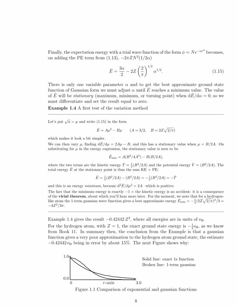
Example 1.4 gives the result −0.42442Z2, where all energies are in units of eH.

For the hydrogen atom, with Z = 1, the exact ground state energy is −12eH, as we know

from Book 11. In summary then, the conclusion from the Example is that a gaussianfunction gives a very poor approximation to the hydrogen atom ground state, the estimate−0.42442 eH being in error by about 15%. The next Figure shows why:

r-axis

1.0

0.00 3.0

Solid line: exact 1s function

Broken line: 1-term gaussian

Figure 1.1 Comparison of exponential and gaussian functions

8

φ(r) fails to describe the sharp cusp when r → 0 and also goes to zero much too rapidlywhen r is large.

Of course we could get the accurate energy E1 = −12eH and the corresponding wave func-

tion φ1, by using a trial function of exponential form exp−ar and varying the parametera until the approximate energy reaches a minimum value. But here we’ll try anotherapproach, taking a mixture of two gaussian functions, one falling rapidly to zero as rincreases and the other falling more slowly: in that way we can hope to correct the maindefects in the 1-term approximation.

Example 1.5 A 2-term gaussian approximation

With a trial function of the form φ = A exp−ar2 + B exp−br2 there are three parameters that canbe independently varied, a, b and the ratio c = B/A – a fourth parameter not being necessary if we’relooking for a normalized function (can you say why?). So we’ll use instead a 2-term function φ =exp−ar2 + c exp−br2.From the previous Examples 1.1-1.3, it’s clear how you can evaluate all the integrals you need in calcu-lating 〈φ|φ〉 and the expectation values 〈φ|V|φ〉, 〈φ|V|φ〉; all you’ll need to change will be the parametervalues in the integrals.

Try to work through this by yourself, without doing the variation of all three values to find the minimum

value of E. (Until you’ve learnt to use a computer that’s much too long a job! But you may like

to know the result: the ‘best’ values of a, b, c are a = 1.32965, b = 0.20146, c = 0.72542 and the

best approximation to E1s then comes out as E = −0.4858Z2eH. This compares with the one-term

approximation E = −0.4244Z2eH; the error is now reduced from about 15% to less than 3%.

The approximate wave function obtained in Example 1.5 is plotted in Figure 1.2 and againcompared with the exact 1s function. (The functions are not normalized, being shiftedvertically to show how well the cusp behaviour is corrected. Normalization improves theagreement in the middle range.)

1.0

0.00.0 3.0 6.0r-axis

Figure 1.2 A 2-term gaussian approximation (broken line)to the hydrogen atom 1s function (solid line)

This Example suggests another form of the variation method, which is both easier to applyand much more powerful. We study it in the next Section, going back to the general case,where Ψ denotes any kind of wave function, expanded in terms of eigenfunctions Ψi.

9

1.3 The linear variation method

Instead of building a variational approximation to the wave function Ψ out of only twoterms we may use as many as we please, taking in general

Ψ = c1Ψ1 + c2Ψ2 + ... + cNΨN , (1.16)

where (with the usual notation) the functions {Ψi (i = 1, 2, ... N)} are ‘fixed’ and we varyonly the coefficients ci in the linear combination: this is called a “linear variation function”and it lies at the root of nearly all methods of constructing atomic and molecular wavefunctions.

From the variation theorem (1.10) we need to calculate the expectation energy E =〈Ψ|H|Ψ〉/〈Ψ|Ψ〉, which we know will give an upper bound to the lowest exact eigenvalueE1 of the operator H. We start by putting this expression in a convenient matrix form:you used matrices a lot in Book 11, ‘representing’ the operator H by a square array ofnumbers H with Hij = 〈Ψi|H|Ψj〉 (called a “matrix element”) standing at the intersectionof the ith row and jth column; and collecting the coefficients ci in a single column c. Amatrix element Hij with j = i lies on the diagonal of the array and gives the expectationenergy Ei when the system is in the particular state Ψ = Ψi. (Look back at Book 11Chapter 7 if you need reminding of the rules for using matrices.)

In matrix notation the more general expectation energy becomes

E =c†Hc

c†Mc, (1.17)

where c† (the ‘Hermitian transpose’ of c) denotes the row of coefficients (c∗1 c∗2, ... c

∗N) and

M (the ‘metric matrix’) looks like H except that Hij is replaced by Mij = 〈Ψi|Ψj〉, thescalar product or ‘overlap’ of the two functions. This allows us to use sets of functionsthat are neither normalized to unity nor orthogonal – with no additional complication.

The best approximate state function (1.11) we can get is obtained by minimizing E tomake it as close as possible to the (unknown!) ground state energy E1, and to do this welook at the effect of a small variation c → c + δc: if we have reached the minimum, Ewill be stationary, with the corresponding change δE = 0.

In the variation c→ c+ δc, E becomes

E + δE =c†Hc+ c†Hδc+ δc†Hc+ ...

c†Mc+ c†Mδc+ δc†Mc+ ...,

where second-order terms that involve products of δ-quantities have been dropped (van-ishing in the limit δc→ 0).

The denominator in this expression can be re-written, since c†Mc is just a number, as

c†Mc[1 + (c†Mc)−1(c†Mδc+ δc†Mc)]

10

and the part in square brackets has an inverse (to first order in small quantities)

1− (c†Mc)−1(c†Mδc+ δc†Mc).

On putting this result in the expression for E + δE and re-arranging a bit (do it!) you’llfind

E + δE = E + c†Mc)−1[(c†Hδc+ δc†Hc)− E(c†Mδc+ δc†Mc)].

It follows that the first-order variation is given by

δE = c†Mc)−1[(c†H− Ec†M)δc+ δc†(Hc− EMc)]. (1.18)

The two terms in (1.18) are complex conjugate, giving a real result which will vanish onlywhen each is zero.

The condition for a stationary value thus reduces to a matrix eigenvalue equation

Hc = EMc. (1.19)

To get the minimum value of E we therefore take the lowest eigenvalue; and the corre-sponding ‘best approximation’ to the wave function Ψ ≈ Ψ1 will follow on solving thesimultaneous equations equivalent to (1.19), namely

∑

j

Hijcj = E∑

j

Mijcj (all i). (1.20)

This is essentially what we did in Example 1.2, where the linear coefficients c1, c2 gave abest approximation when they satisfied the two simultaneous equations

(H11 − EM11)c1 + (H12 − EM12)c2 = 0,

(H21 − EM21)c1 + (H22 − EM22)c2 = 0,

the other parameters bing fixed. Now we want to do the same thing generally, using alarge basis of N expansion functions {Ψi}, and to make the calculation easier it’s best touse an orthonormal set. For the case N = 2, M11 = M22 = 1 and M12 = M21 = 0, theequations then become

(H11 − E)c1 = −H12c2,

H21c1 = −(H22 − E)c2.

Here there are three unknowns, E, c1, c2. However, by dividing each side of the firstequation by the corresponding side of the second, we can eliminate two of them, leavingonly

(H11 − E)H21

=H12

(H22 − E).

This is quadratic in E and has two possible solutions. On ‘cross-multiplying’ it followsthat (H11 − E)(H22 − E) = H12H21 and on solving we get lower and upper values E1

11

and E2. After substituting either value back in the original equations, we can solve to getthe ratio of the expansion coefficients. Normalization to make c21 + c22 = 1 then results inapproximations to the first two wave functions, Ψ1 (the ground state) and Ψ2 (a state ofhigher energy).

Generalization

Suppose we want a really good approximation and use a basis containing hundreds offunctions Ψi. The set of simultaneous equations to be solved will then be enormous; butwe can see how to continue by looking at the case N = 3, where they become

(H11 − EM11)c1 + (H12 − EM12)c2 + (H13 − EM13)c3 = 0,

(H21 − EM21)c1 + (H22 − EM22)c2 + (H23 − EM23)c3 = 0,

(H31 − EM31)c1 + (H32 − EM32)c2 + (H33 − EM33)c3 = 0.

We’ll again take an orthonormal set, to simplify things. In that case the equations reduceto (in matrix form)

H11 − E H12 H13

H21 H22 − E H23

H31 H32 H33 − E

c1c2c3

=

000

.

When there were only two expansion functions we had similar equations, but with onlytwo rows and columns in the matrices:

(

H11 − E H12

H21 H22 − E

)(

c1c2

)

=

(

00

)

.

And we got a solution by ‘cross-multiplying’ in the square matrix, which gave

(H11 − E)(H22 − E)−H21H12 = 0.

This is called a compatibility condition: it determines the only values of E for whichthe equations are compatible (i.e. can both be solved at the same time).

In the general case, there are N simultaneous equations and the condition involves thedeterminant of the square array: thus for N = 3 it becomes

∣

∣

∣

∣

∣

∣

H11 − E H12 H13

H21 H22 − E H23

H31 H32 H33 − E

∣

∣

∣

∣

∣

∣

= 0. (1.21)

There are many books on algebra, where you can find whole chapters on the theory ofdeterminants, but nowadays equations like (1.16) can be solved easily with the help ofa small computer. All the ‘theory’ you really need, was explained long ago in Book 2(Section 6.12). So here a reminder should be enough:

12

Given a square matrix A, with three rows and columns, its determinant can be evaluated as follows. Youcan start from the 11-element A11 and then get the determnant of the 2×2 matrix that is left when youtake away the first row and first column:

∣

∣

∣

∣

A22 A23

A32 A33

∣

∣

∣

∣

= A22A33 −A32A23.

– as follows from what you did just before (1.16). What you have evaluated is called the ‘co-factor’ ofA11 and is denoted by A(11).

Then move to the next element in the first row, namely A12, and do the same sort of thing: take awaythe first row and second column and then get the determinant of the 2×2 matrix that is left. This wouldseem to be the co-factor of A12; but in fact, whenever you move from one element in the row to the next,you have to attach a minus sign; so what you have found is −A(12).

When you’ve finished the row you can put together the three contributions to get

|A| = A11A(11) −A12A

(12) +A13A(13)

and you’ve evaluated the 3×3 determinant!

The only reason for reminding you of all that (since a small computer can do such thingsmuch better than we can) was to show that the determinant in (1.21) will give you apolynomial of degree 3 in the energy E. (That is clear if you take A = H− E1, make theexpansion, and look at the terms that arise from the product of elements on the ‘principaldiagonal’, namely (H11− E)× (H22− E)× (H33− E). These include −E3.) Generally, asyou can see, the expansion of a determinant like (1.16), but with N rows and columns,will contain a term of highest degree in E of the form (−1)N EN . This leads to conclusionsof very great importance – as you’re just about to see.

1.4 Going all the way! Is there a limit?

The first time you learnt anything about eigenfunctions and how they could be usedwas in Book 3 (Section 6.3). Before starting the present Section 1.4 of Book 12, youshould read again what was done there. You were studying a simple differential equation,the one that describes standing waves on a vibrating string, and the solutions were sinefunctions (very much like the eigenfunctions coming from Schrodinger’s equation for a‘particle in a box’, discussed in Book 11). By putting together a large number of suchfunctions, corresponding to increasing values of the vibration frequency, you were able toget approximations to the instantaneous shape of the string for any kind of vibration.That was a first example of an eigenfunction expansion. Here we’re going to use suchexpansions in constructing approximate wave functions for atoms and molecules; andwe’ve taken the first steps by starting from linear variation functions. What we must donow is to ask how a function of the form (1.16) can approach more and more closely anexact eigenfunction of the Hamiltonian H as N is increased.

In Section 1.3 it was shown that an N -term variation function (1.16) could give an op-timum approximation to the ground state wave function Ψ1, provided the expansioncoefficients ci were chosen so as to satisfy a set of linear equations: for N = 3 these took

13

the form

(H11 − EM11)c1 + (H12 − EM12)c2 + (H13 − EM13)c3 = 0,

(H21 − EM21)c1 + (H22 − EM22)c2 + (H23 − EM23)c3 = 0,

(H31 − EM31)c1 + (H32 − EM32)c2 + (H33 − EM33)c3 = 0.

and were compatible only when the variational energy E satisfied the condition (1.16).There are only three values of E which do so. We know that E1 is an upper bound to theaccurate lowest-energy eigenvalue E1 but what about the other two?

In general, equations of this kind are called secular equations and a condition like (1.16)is called a secular determinant. If we plot the value, ∆ say, of the determinant (havingworked it out for any chosen value of E) against E, we’ll get a curve something like theone in Figure 1.3; and whenever the curve crosses the horizontal axis we’ll have ∆ = 0,the compatibility condition will be satisfied and that value of E will allow you to solvethe secular equations. For other values you just can’t do it!

∆(E)

E

Figure 1.3 Secular determinantSolid line: for N = 3Broken line: for N = 4

E

E1

E2

E3

E1

E2

E3

E4

E1

Figure 1.4 Energy levelsSolid lines: for N = 3Broken lines: for N = 4

On the far left in Fig.1.3, ∆ will become indefinitely large and positive because its ex-pansion is a polynomial dominated by the term −E3 and E is negative. On the otherside, where E is positive, the curve on the far right will go off to large negative values. Inbetween there will be three crossing points, showing the acceptable energy values.

Now let’s look at the effect of increasing the number of basis functions by adding another,Ψ4. The value of the secular determinant then changes and, since expansion gives apolynomial of degree 4, it will go towards +∞ for large values of E. Figure 1.3 shows thatthere are now four crossing points on the x-axis and therefore four acceptable solutionsof the secular equations. The corresponding energy levels for N = 3 and N = 4 arecompared in Figure 1.4, where the first three are seen to go down, while one new level(E4) appears at higher energy. The levels for N = 4 fall in between the levels above andbelow for N = 3 and this result is often called the “separation theorem”: it can be provedproperly by studying the values of the determinant ∆N(E) for values of E at the crossingpoints of ∆N−1(E).

14

The conclusion is that, as more and more basis functions are added, the roots of thesecular determinant go steadily (or ‘monotonically’) down and will therefore approachlimiting values. The first of these, E1, is known to be an upper bound to the exact lowesteigenvalue of H (i.e. the groundstate of the system) and it now appears that the higherroots will give upper bounds to the higher ‘excited’ states. For this conclusion to be trueit is necessary that the chosen basis functions form a complete set.

1.5 Complete set expansions

So far, in the last section, we’ve been thinking of linear variation functions in general,without saying much about the forms of the expansion functions and how they can beconstructed; but for atoms and molecules they may be functions of many variables (e.g.coordinates x1, y1, z1, x2, y2, z2, x3, ... zN for N particles – even without including spins!).From now on we’ll be dealing mainly with wave functions built up from one-particlefunctions, which from now on we’ll denote by lower-case letters {φk(ri)} with the index ilabelling ‘Particle i’ and ri standing for all three variables needed to indicate its positionin space (spin will be put in later); as usual the subscript on the function will just indicatewhich one of the whole set (k = 1, 2, ... n) we mean. (It’s a pity so many labels are needed,and that sometimes we have to change their names, but by now you must be getting usedto the fact that you’re playing a difficult game – once you’re clear about what the symbolsstand for the rest will be easy!)

Let’s start by thinking again of the simplest case; one particle, moving in one dimension,so the particle label i is not needed and r can be replaced by just one variable, x. Insteadof φk(ri) we can then use φk(x). We want to represent any function f(x) as a linearcombination of these basis functions and we’ll write

f (n)(x) = c1φ1(x) + c2φ2(x) + ... + cnφn(x) (1.22)

as the ‘n-term approximation’ to f(x).

Our first job will be to choose the coefficients so as to get a best approximation to f(x)over the whole range of x-values (not just at one point). And by “the whole range” we’llmean for all x in the interval, (a, b) say, outside which the function has values that canbe neglected: the range may be very small (think of the delta-function you met in Book11) or very large (think of the interval (−∞,+∞) for a particle moving in free space).(When we need to show the limits of the interval we’ll just use x = a and x = b.)

Generally, the curves we get on plotting f(x) and f (n)(x) will differ and their differencecan be measured by ∆(x) = f(x) − f (n)(x) at all points in the range. But ∆(x) willsometimes be positive and sometimes negative. So it’s no good adding these differencesfor all points on the curve (which will mean integrating ∆(x)) to get a measure of howpoor the approximation is; for cancellations could lead to zero even when the curves werevery different. It’s really the magnitude of ∆(x) that matters, or its square – which isalways positive.

15

So instead let’s measure the difference by |f(x) − f (n)(x)|2, at any point, and the ‘totaldifference’ by

D =

∫ b

a

∆(x)2dx =

∫ b

a

|f(x)− f (n)(x)|2dx. (1.23)

The integral gives the sum of the areas of all the strips between x = a and x = b ofheight ∆2 and width dx. This quantity will measure the error when the whole curve isapproximated by f (n)(x) and we’ll only get a really good fit, over the whole range of x,when D is close to zero.

The coefficients ck should be chosen to give D its lowest possible value and you knowhow to do that: for a function of one variable you find a minimum value by first seekinga ‘turning point’ where (df/dx) = 0; and then check that it really is a minimum, byverifying that (d2f/dx2) is positive. It’s just the same here, except that we look atthe variables one at a time, keeping the others constant. Remember too that it’s thecoefficients ck that we’re going to vary, not x.

Now let’s put (1.17) into (1.18) and try to evaluate D. You first get (dropping the usualvariable x and the limits a, b when they are obvious)

D =

∫

|f − f (n)|2dx =

∫

f 2dx+

∫

(f (n))2dx− 2

∫

ff (n)dx. (1.24)

So there are three terms to differentiate – only the last two really, because the firstdoesn’t contain any ck and so will disappear when you start differentiating. These twoterms are very easy to deal with if you make use of the supposed orthonormality of theexpansion functions: for real functions

∫

φ2kdx = 1,

∫

φkφldx = 0 (k 6= l). Using thesetwo properties, we can go back to (1.19) and differentiate the last two terms, with respectto each ck (one at a time, holding the others fixed): the first of the two terms leads to

∂

∂ck

∫

(f (n))2dx =∂

∂ckc2k

∫

φk(x)2dx = 2ck;

while the second one gives

−2 ∂

∂ck

∫

ff (n)dx = −2 ∂

∂ckck

∫

f(x)φk(x)dx = −2〈f |φk〉,

where Dirac notation (see Chapter 9 of Book 11) has been used for the integral∫

f(x)φk(x)dx,which is the scalar product of the two functions f(x) and φk(x):

〈f |φk〉 =∫

f(x)φk(x)dx.

We can now do the differentiation of the whole difference function D in (1.18). The resultis

∂D

∂ck= 2ck − 2〈f |φk〉

16

and this tells us immediately how to choose the coefficients in the n-term approximation(1.17) so as to get the best possible fit to the given function f(x): setting all the derivativesequal to zero gives

ck = 〈f |φk〉 (for all k). (1.25)

So it’s really very simple: you just have to evaluate one integral to get any coefficientyou want. And once you’ve got it, there’s never any need to change it in getting a betterapproximation. You can make the expansion as long as you like by adding more terms,but the coefficients of the ones you’ve already done are final. Moreover, the results arequite general: if you use basis functions that are no longer real you only need change thedefinition of the scalar product, taking instead the Hermitian scalar product as in (1.1).

Generalizations

In studying atoms and molecules we’ll have to deal with functions of very many variables,not just one. But some of the examples we met in Book 11 suggest possible ways ofproceeding. Thus, in going from the harmonic oscillator in one dimension (Example 4.3),with eigenfunctions Ψk(x), to the 3-dimensional oscillator (Example 4.4) it was possibleto find eigenfunctions of product form, each of the three factors being of 1-dimensionalform. The same was true for a particle in a rectangular box; and also for a free particle.

To explore such possibilities more generally we first ask if a function of two variables, xand x′, defined for x in the interval (a, b) and x′ in (a′, b′), can be expanded in productsof the form φi(x)φ

′j(x

′). Suppose we write (hopefully!)

f(x, x′) =∑

i,j

cijφi(x)φ′j(x

′) (1.26)

where the set {φi(x)} is complete for functions of x defined in (a, b), while {φ′i(x

′)} iscomplete for functions of x′ defined in (a′, b′). Can we justify (1.26)? A simple argumentsuggests that we can.

For any given value of the variable x′ we may safely take (if {φi(x)} is indeed complete)

f(x, x′) = c1φ1(x) + c2φ2(x) + ... ciφi(x) + ....

where the coefficients must depend on the chosen value of x′. But then, because {φ′i(x

′)}is also supposed to be complete, for functions of x′ in the interval (a′, b′), we may expressthe general coefficient ci in the previous expansion as

ci = ci1φ′1(x

′) + ci2φ′2(x

′) + ...cijφj(x′) + ....

On putting this expression for ci in the first expansion we get the double summation pos-tulated in (1.26) (as you should verify!). If the variables x, x′ are interpreted as Cartesiancoordinates the expansion may be expected to hold good within the rectangle boundedby the summation limits.

Of course, this argument would not satisfy any pure mathematician; but the furthergeneralizations it suggests have been found satisfactory in a wide range of applications in

17

Applied Mathematics and Physics. In the quantum mechanics of many-electron systems,for example, where the different particles are physically identical and may be describedin terms of a single complete set, the many-electron wave function is commonly expandedin terms of products of 1-electron functions (or ‘orbitals’).

Thus, one might expect to find 2-electron wave functions constructed in the form

Ψ(r1, r2) =∑

i,j

ci,jφi(r1)φj(r2),

where the same set of orbitals {φi} is used for each of the identical particles, the twofactors in the product being functions of the different particle variables r1, r2. Here aboldface letter r stands for the set of three variables (e.g. Cartesian coordinates) definingthe position of a particle at point r. The labels i and j run over all the orbitals of the (inprinciple) complete set, or (in practice) over all values 1, 2, 3, .... n, in the finite set usedin constructing an approximate wave function.

In Chapter 2 you will find applications to 2-electron atoms and molecules where the wavefunctions are built up from one-centre orbitals of the kind studied in Book 11. (You canfind pictures of atomic orbitals there, in Chapter 3.)

18

Chapter 2

Some two-electron systems

2.1 Going from one particle to two

For two electrons moving in the field provided by one or more positively charged nuclei(supposedly fixed in space), the Hamiltonian takes the form

H(1, 2) = h(1) + h(2) + g(1, 2) (2.1)

where H(1, 2) operates on the variables of both particles, while h(i) operates on those ofParticle i alone. (Don’t get mixed up with names of the indices – here i = 1, 2 label thetwo electrons.) The one-electron Hamiltonian h(i) has the usual form (see Book 11)

h(i) = −12∇2(i) + V (i), (2.2)

the first term being the kinetic energy (KE) operator and the second being the potentialenergy (PE) of Electron i in the given field. The operator g(1, 2) in (2.1) is simply theinteraction potential, e2/κ0rij , expressed in ‘atomic units’ (see Book 11) 1 So in (2.1) wetake

g(1, 2) = g(1, 2) =1

r12, (2.3)

r12 being the inter-electron distance. To get a very rough estimate of the total energy E,we may neglect this term altogether and use an approximate Hamiltonian

H0(1, 2) = h(1) + h(2), (2.4)

which describes an Independent Particle ‘Model’ of the system. The resultant IPMapproximation is fundamental to all that will be done in Book 12.

1A fully consistent set of units on an ‘atomic’ scale is obtained by taking the mass and charge ofthe electron (m, e) to have unit values, along with the action ~ = h/2π. Other units are κ0 = 4π ǫ0 (ǫ0being the “electric permittivity of free space”); length a0 = ~

2κ0/me2 and energy eH = me4/κ 2

0 ~2.

These quantities may be set equal to unity wherever they appear, leading to a great simplification of allequations. If the result of an energy calculation is the number x this just means that E = xeH; similarlya distance calculation would give L = xa0.

19

With a Hamiltonian of this IPM form we can look for a solution of product form anduse the ‘separation method’ (as in Chapter 4 of Book 11). We therefore look for a wavefunction Ψ(r1, r2) = φm(r1)φn(r2). Here each factor is a function of the position variablesof only one of the two electrons, indicated by r1 or r2, and (to be general!) Electron 1 isdescribed by a wave function φm while Electron 2 is described by φn.

On substituting this product in the eigenvalue equation H0Ψ = EΨ and dividing through-out by Ψ you get (do it!)

h(1)φm(r1)

φm(r1)+

h(2)φn(r2)

φn(r2)= E.

Now the two terms on the left-hand side are quite independent, involving different sets ofvariables, and their sum can be a constant E, only if each term is separately a constant.Calling the two constants ǫm and ǫn, the product Ψmn(r1, r2) = φm(r1)φn(r2) will satisfythe eigenvalue equation provided

h(1)φm(r1) = ǫmφm(r1),

h(2)φn(r2) = ǫnφn(r2).

The total energy will then beE = ǫm + ǫn. (2.5)

This means that the orbital product is an eigenfunction of the IPM Hamiltonian pro-vided φm and φn are any solutions of the one-electron eigenvalue equation

hφ(r) = ǫφ(r). (2.6)

Note especially that the names given to the electrons, and to the corresponding variablesr1 and r2, don’t matter at all. The same equation applies to each electron and φ = φ(r)is a function of position for whichever electron we’re thinking of: that’s why the labels 1and 2 have been dropped in the one-electron equation (2.6). Each electron has ‘its own’orbital energy, depending on which solution we choose to describe it, and since H0 in(2.4) does not contain any interaction energy it is not surprising that their sum gives thetotal energy E. We often say that the electron “is in” or “occupies” the orbital chosen todescribe it. If Electron 1 is in φm and Electron 2 is in φn, then the two-electron function

Ψmn(r1, r2) = φm(r1)φn(r2)

will be an exact eigenfunction of the IPM Hamiltonian (2.4), with eigenvalue (2.5).

For example, putting both electrons in the lowest energy orbital, φ1 say, gives a wavefunction Ψ11(r1, r2) = φ1(r1)φ1(r2) corresponding to total energy E = 2ǫ1. This is the(strictly!) IPM description of the ground state of the system. To improve on thisapproximation, which is very crude, we must allow for electron interaction: the nextapproximation is to use the full Hamiltonian (2.1) to calculate the energy expectationvalue for the IPM function (no longer an eigen-function of H). Thus

Ψ11(r1, r2) = φ1(r1)φ1(r2). (2.7)

20

and this gives

E = 〈Ψ11|h(1) + h(2) + g(1, 2)|Ψ11〉 = 2〈φ1|h|φ1〉+ 〈φ1φ1|g|φ1φ1〉, (2.8)

where the first term on the right is simply twice the energy of one electron in orbital φ1,namely 2ǫ1. The second term involves the two-electron operator given in (2.3) and hasexplicit form

〈φ1φ1|g|φ1φ1〉 =∫

φ∗1(r1)φ

∗1(r2)

1

r12φ1(r1)φ1(r2)dr1dr2, (2.9)

Here the variables in the bra and the ket will always be labelled in the order 1,2 and thevolume element dr1, for example, will refer to integration over all particle variables (e.g.in Cartesian coordinates it is dx1dy1dz1). (Remember also that, in bra-ket notation, thefunctions that come from the bra should in general carry the star (complex conjugate);and even when the functions are real it is useful to keep the star.)

To evaluate the integral we need to know the form of the 1-electron wave function φ1, butthe expression (2.9) is a valid first approximation to the electron repulsion energy in theground state of any 2-electron system.

Let’s start with the Helium atom, with just two electrons moving in the field of a nucleusof charge Z = 2.

2.2 The Helium atom

The function (2.7) is clearly normalized when, as we suppose, the orbitals themselves(which are now atomic orbitals) are normalized; for

〈φ1φ1|φ1φ1〉 =∫

φ∗1(r1)φ

∗1(r2)φ1(r1)φ1(r2)dr1dr2 = 〈φ1|φ1〉 〈φ1|φ1〉 = 1× 1.

The approximate energy (2.8) is then

E = 2ǫ1 + 〈φ1φ1|g|φ1φ1〉 = 2ǫ1 + J11, (2.10)

Here ǫ1 is the orbital energy of an electron, by itself, in orbital φ1 in the field of the nucleus;the 2-electron term J11 is often called a ‘Coulomb integral’ because it corresponds to theCoulombic repulsion energy (see Book 10) of two distributions of electric charge, eachof density |φ1(r)|2 per unit volume. For a hydrogen-like atom, with atomic number Z,we know that ǫ1 = −1

2Z2eH. When the Coulomb integral is evaluated it turns out to

be J11 = (5/8)ZeH and the approximate energy thus becomes E = −Z2 + (5/8)Z in‘atomic’ units of eH. With Z = 2 this gives a first estimate of the electronic energy of theHelium atom in its ground state: E = −2.75 eH, compared with an experimental value−2.90374 eH.To improve the ground state wave function we may use the variation method as in Section1.2 by choosing a new function φ′

1 = N ′e−Z′r, where Z ′ takes the place of the actual nuclear

21

charge and is to be treated as an adjustable parameter. This allows the electron to ‘feel’an ‘effective nuclear charge’ a bit different from the actual Z = 2. The correspondingnormalizing factor N ′ will have to be chosen so that

〈φ′1|φ′

1〉 = N ′2

∫

exp(−2Z ′r)(4πr2)dr = 1

and this gives (prove it!) N ′2 = Z ′3/π.

The energy expectation value still has the form (2.8) and the terms can be evaluatedseparately

Example 2.1 Evaluation of the one-electron term

The first 1-electron operator has an expectation value 〈Ψ11|h(1)|Ψ11〉 = 〈φ′1|h|φ′1〉〈φ′1|φ′1〉, a matrix ele-ment of the operator h times the scalar product 〈φ′1|φ′1〉. In full, this is

〈Ψ11|h(1)|Ψ11〉 = N ′2

∫ ∞

0

e−Z′rhe−Z′r4πr2dr ×N ′2

∫ ∞

0

e−Z′re−Z′r4πr2dr,

where h working on a function of r alone is equivalent to (− 12∇2−Z/r) – h containing the actual charge

(Z).

We can spare ourselves some work by noting that if we put Z = Z ′ the function φ′1 = N ′e−Z′r becomesan eigenfunction of (− 1

2∇2 − Z ′/r) with eigenvalue ǫ′ = − 12Z

′2 (Z ′ being a ‘pretend’ value of Z. So

h = − 12∇2 − Z/r = (− 1

2∇2 − Z ′/r) + (Z ′ − Z)/r,

where the operator in parentheses is easy to handle: when it works on φ′1 it simply multiplies it by theeigenvalue − 1

2Z′2. Thus, the operator h, working on the function N ′e−Z′r gives

h(N ′e−Z′r) =(

− 12Z

′2 + Z′−Zr

)

N ′e−Z′r.

The one-electron part of (2.8) can now be written as (two equal terms – say why!) 2〈Ψ11|h(1)|Ψ11〉 where

〈Ψ11|h(1)|Ψ11〉 = 〈φ′1|h|φ′1〉〈φ′1|φ′1〉

= N ′2

∫ ∞

0

e−Z′rhe−Z′r4πr2dr ×N ′2

∫ ∞

0

e−2Z′r4πr2dr

= N ′2

∫ ∞

0

e−Z′r(

− 12Z

′2 + Z′−Zr

)

e−Z′r4πr2dr.

Here the last integral on the second line is unity (normalization) and leaves only the one before it. Thisremaining integration gives (check it out!) 〈Ψ11|h(1)|Ψ11〉 = − 1

2Z′2 +4π(Z ′−Z)N ′2

∫∞

0(re−2Z′r)dr and

from the simple definite integral∫∞

0xe−axdx = (1/a2) it follows that

〈Ψ11|h(1)|Ψ11〉 = − 12Z

′2 + 4π(Z ′ − Z)N ′2(1/2Z ′)

and since N ′2 = Z ′3/π the final result is

〈Ψ11|h(1)|Ψ11〉 = − 12Z

′2 + Z ′(Z ′ − Z).

22

Example 2.1 has given the expectation value of the h(1) term in (2.8), but h(2) must givean identical result since the only difference is a change of electron label from 1 to 2; andthe third term must have the value J ′

11 = (5/8)Z ′ since the nuclear charge Z has beengiven the varied value Z ′ only in the orbital exponent (nothing else being changed).

On putting these results together, the energy expectation value after variation of theorbital exponent will be

E = −Z ′2 + 2Z ′(Z ′ − Z) + (5/8)Z ′ (2.11)

– all, as usual, in energy units of eH.

The variational calculation can now be completed: E will be stationary when

dE

dZ ′= −2Z ′ + 4Z ′ − 2Z + (5/8) = 0

and this means that the best estimate of the total electronic energy will be found onreducing the orbital exponent from its value Z = 2 for one electron by itself to the valueZ ′ = 2− (5/16) in the presence of the second electron. In other words, the central field iseffectively reduced or ‘screened’ when it holds another electron: the screening constant

(5/16) is quite large and the ground state orbital expands appreciably as a result of thescreening.

The corresponding estimate of the ground state energy is

E = −(27/16)2 = −2.84765 eH (2.12)

– a value which compares with −2.75 eH before the variation of Z and is much closer tothe ‘exact’ value of −2.90374 eH obtained using a very elaborate variation function.

Before moving on, we should make sure that the value used for the Coulomb integralJ = (5/8)ZeH is correct2. This is our first example of a 2-electron integral: for twoelectrons in the same orbital φ it has the form (2.9), namely (dropping the orbital label‘1’)

J =

∫

φ∗(r1)φ∗(r2)

1

r12φ(r1)φ(r2)dr1dr2.

To evaluate it, we start from Born’s interpretation of the wave function |φ(r)|2 = φ∗(r)φ(r)(the star allowing the function to be complex ) as a probability density. It is theprobability per unit volume of finding the electron in a small element of volume dr atPoint r and will be denoted by ρ(r) = φ∗(r)φ(r). As you know from Book 11, thisinterpretation is justified by countless experimental observations.

We now go a step further: the average value of any quantity f(r) that depends only on theinstantaneous position of the moving electron will be given by f =

∫

f(r)ρ(r)dr where,as usual, the integration is over all space (i.e. all values of the electronic variables). Nowthe electron carries a charge −e and produces a potential field Vr′ at any chosen ‘fieldpoint’ r′.

2If you find the proof too difficult, just take the result on trust and keep moving!

23

It’s convenient to use r1 for the position of the electron (instead of r) and to use r2 forthe second point, at which we want to get the potential Vr2 . This will have the valueVr2 = −e/κ0|r21|, where |r21| = |r12| = r12 is the distance between the electron at r1 andthe field point r2.

When the electron moves around, its position being described by the probability densityρ(r1), the electric potential it produces at any point r′ will then have an average value

V (r2) =−eκ0

∫

1

|r21|dρ(r1)r1.

In words, this means that

The average electric field at point r2, produced by anelectron at point r1 with probability density ρ(r1), canthen be calculated just as if the ‘point’ electron were‘smeared out’ in space, with a charge density −eρ(r1).

(2.13)

The statement (2.13) provides the charge cloud picture of the probability density. Itallows us to visualize very clearly, as will be seen later, the origin of many properties ofatoms and molecules. As a first application let’s look at the Coulomb integral J.

Example 2.2 Interpretation of the electron interaction.

The integral J can now be viewed as the interaction energy of two distributions of electric charge, bothof density −eρ(r) and of spherical form (one on top of the other). (If that seems like nonsense rememberthis is only a mathematical interpretation!)

The two densities are in this case ρ1(r1) = N2 exp−2Zr 21 and ρ2(r2) = N2 exp−2Zr 2

2 ; and the integralwe need follows on putting the interaction potential V (r1, r2) = 1/r12 between the two and integratingover all positions of both points. Thus, giving e and κ0 their unit values, J becomes the double integral

J = ZN4

∫ ∫

exp−2Zr 21

1

r12exp−2Zr 2

2 dr1dr2,

where (1/r12) is simply the inverse distance between the two integration points. On the other hand,dr1 and dr2 are 3-dimensional elements of volume; and when the charge distributions are sphericallysymmetrical functions of distance (r1, r2) from the origin (the nucleus), they may be divided into sphericalshells of charge. The density is then constant within each shell, of thickness dr; and each holds a totalcharge 4πr2dr × ρ(r), the density being a function of radial distance (r) alone.

Now comes a nice connection with Electrostatics, which you should read about again in Book 10, Section1.4. Before going on you should pause and study Figure 2.2, to have a clear picture of what we must donext.

Example 2.2 perhaps gave you an idea of how difficult it can be to deal with 2-electronintegrals. The diagram below will be helpful if you want to actually evaluate J , thesimplest one we’ve come across.

24

r1

r

r2

r12

Figure 2.2 Spherical shells of electron density (blue)

The integral J gives the electrostatic potential energy of two spherical charge distributions.Each could be built up from spherical ‘shells’ (like an onion): these are shown in blue, onefor Electron 1 having radius r1 and another for Electron 2 with radius r2. The distancebetween the two shells is shown with label r12 and this determines their potential energyas the product of the total charges they contain (4πr 2

1 dr1 and 4πr 22 dr2) times the inverse

distance (r−112 ). The total potential energy is obtained by summing (integrating) over all

shells – but you need a trick! at any distance r from the nucleus, the potential due to aninner shell (r1 < r) is constant until r1 reaches r and changes form; so the first integrationbreaks into two parts, giving a result which depends only on where you put r (indicatedby the broken line).

Example 2.3 Evaluation of the electron interaction integral, J

To summarize, J arises as the interaction energy of all pairs of spherical shells of charge, shown (blue) inFigure 2.2, and this will come from integration over all shells. We take one pair at a time.

You know from Book 10 that the electrostatic potential at distance r from the origin (call it V (r)) dueto a spherical shell of charge, of radius r1, is given by

V (r) = Qr1 ×1

r1for r < r1,

= Qr1 ×1

rfor r > r1,

where Qr1 = 4πr 21 dr1×ρ(r1) is the total charge contained in the shell of radius r1 and thickness dr1. The

potential is thus constant within the first shell; but outside has a value corresponding to all the chargebeing put at the origin.

We can now do the integration over the variable r1 as it goes from 0 to ∞. For r1 < r the sum of thecontributions to J from the shells within a sphere of radius r will be

(1/r)

∫ r

0

exp(−2Zr 21 )4πr

21 dr1, (A)

25

while for r1 > r the rest of the r1 integration will give the sum of contributions from shells of radiusgreater than r, namely

∫ ∞

r

exp(−2Zr 21 )(1/r1)4πr

21 dr1. (B)

You’ve met integrals a bit like these in Chapter 1, so you know how to do them and can show (do it!)that the sum of A and B is the potential function

V (r) =4π

r[2− e−r(2 + r)].

This is a function of r alone, the radius of the imaginary sphere that we used to separate the integrationover r1 into two parts, so now we can put r = r2 and multiply by (4πr 2

2 dr2)Ne−r2 to obtain the energy

of one shell of the second charge distribution in the field generated by the first.

After that it’s all plain sailing: the integration over all the outer shells (r2) now goes from 0 to ∞ – andyou’re home and dry! Integration over r2, for all shells from r2 = 0 to ∞, will then give (check it out!)

J =Z

2

∫ ∞

0

[2− e−r2(2 + r2)]e−r2r2dr2 = (5/8)Z.

Example 2.3 gave you a small taste of how difficult it can be to actually evaluate the2-electron integrals that are needed in describing electron interactions.

Now you know how to get a decent wave function for two electrons moving in the fieldof a single nucleus – the helium atom – and how the approximation can be improved asmuch as you wish by using the variation method with more elaborate trial functions. Butfollowing that path leads into difficult mathematics; so instead let’s move on and take aquick look at some excited states.

First excited states of He

In Book 11 we studied central-field systems, including many-electron atoms, in order toillustrate the general principles of quantum mechanics. In particular, we looked for sets ofcommuting operators associated with observable quantities such as angular momentum,finding that the angular momentum operators for motion in a central field commuted withthe Hamiltonian H (see Chapter 6 of Book 11) and could therefore take simultaneouslydefinite eigenvalues, along with the energy. For such a system, the energy eigenstates couldbe grouped into series, according to values of the angular momentum quantum numbersL and M which determine the angular momentum and one of its three components.

But here we are dealing with systems of at most two electrons and the general theory isnot needed: a 2-electron wave function is represented approximately as a product of 1-electron orbitals. And for the Helium atom we are dealing with spherically symmetricalwave functions, which involve only ‘s-type’ orbitals, with zero angular momentum.

As a first example of an excited state we suppose one of the two electrons in the groundstate, with wave function Ψ11(r1, r2) = φ1(r1)φ2(r2), is ‘promoted’ into the next higherorbital φ2 of the s series. According to equation (6.10) of Book 11 Chapter 6, this AOcorresponds to energy E2 = −1

2(Z2/4), the whole series being depicted in Figure 13.

26

Example 2.4 Excited state wave functions and energies

When one of the two electrons is promoted from the lowest-energy AO φ1 into the next one, φ2, thereare clearly two distinct ways of representing the state by an IPM function: it could be either

Ψ12(r1, r2) = φ1(r1)φ2(r2),

in which Electron 2 has been promoted, or

Ψ21(r1, r2) = φ2(r1)φ1(r2),

in which Electron 1 (with coordinates r1) has been put into φ2, the second electron staying in φ1. Andat this point three product functions are available for constructing 2-electron wave functions – those wehave called Ψ11, the IPM ground state, and Ψ12,Ψ21, in which one of the electrons has been promoted.We could of course set up other products Ψlm, with both electrons promoted to higher-energy AOs, andsuppose these may be used in the first few terms of a complete set expansion of the 2-electron wavefunction. The products corresponding to any particular choice of the orbitals e.g. φ1, φ2 are said tobelong to the same electron configuration.

Here, to simplify things, we’ll use a single-subscript notation to denote the first three products: Ψ1 =φ1φ1, Ψ2 = φ1φ2, Ψ3 = φ2φ1,We can then use the linear variation method (Section 1.3) to get improvedapproximations to the three lowest-energy wave functions in the form

Ψ = c1Ψ1 + c2Ψ2 + c3Ψ3.

This involves setting up the secular equations

(H11 − EM11)c1 + (H12 − EM12)c2 + (H13 − EM13)c3 = 0,

(H21 − EM21)c1 + (H22 − EM22)c2 + (H23 − EM23)c3 = 0,

(H31 − EM31)c1 + (H32 − EM32)c2 + (H33 − EM33)c3 = 0,

where, as usual, Hij = 〈Ψi|H|Ψj〉 and Mij = 〈Ψi|Ψj〉. On solving them we obtain, along with theoptimized mixtures, improved approximations to the energies E1, E2, E3 of the first three electronicstates. (Read Section 1.3 again if you need to.)

Here, the approximate ground-state function Ψ1 has a very small overlap with Ψ2 and Ψ3; for example

M12 = 〈Ψ1|Ψ2〉 = 〈φ1φ1|φ1φ2〉 = 〈φ1|φ1〉〈φ1|φ2〉 ≈ 0,

because 〈φ1|φ1〉 = 1 and 〈φ1|φ2〉 ≈ 0 – the 1s and 2s AOs being normalized and lying mainly in differentregions of space. For similar reasons, other off-diagonal terms such as H12, H13, which connect the IPMground state Ψ1 with the higher-energy functions Ψ2, Ψ3 are usually small enough to be neglected.

With such approximations (check them out!) the secular equations may be written

(H11 − E)c1 = 0,

(H22 − E)c2 = −H23c3,

H32c2 = −(H33 − E)c3.

The first equation says that E ≈ H11 is still an approximation to the ground-state energy E1. The otherequations allow us to eliminate the expansion coefficients and to determine approximate eigenvalues fortwo excited states. Thus (you’ve done it all before in Section 1.3 !), on dividing each side of the secondequation by the corresponding side of the third, the coefficients cancel and leave you with

(H22 − E)

H32=

H23

(H33 − E).

27

Now we know that H22 = H33 (say why!) and H32 = H23 (real matrix elements) and if we call thesequantities α and β the equation becomes (α− E)2 = β2. The two roots are (α− E) = ±β and give twoapproximate excited-state energies: E(+) = α+ β and E(−) = α− β.To end this example let’s get the energies of these states, just as we did for the ground state, where wefound E = 2ǫ1 + J11 in terms of orbital energy ǫ1 and Coulomb interaction J11. (You should read again,from equation (2.7) to equation (2.8), to remind yourself of how we did it.)

The excited states are linear combinations of the functions Ψ2,Ψ3, which belong to the configuration

1s2s. Thus Ψ(+)2 for the ‘plus combination’, with energy E

(+)2 , is obtained by putting E

(+)2 = α + β

back into the second equation, which shows that c3 = c2. This state therefore has the (normalized) form

Ψ(+)2 = (Ψ2 +Ψ3)/

√2 and Ψ

(−)2 will be similar, with the plus changed to a minus.

The energy expectation value in state Ψ(+)2 will be 〈Ψ (+)

2 |H|〈Ψ(+)2 〉 = 1

2 [H22 + H33 + 2H23], whereH22 = H33 = 〈Ψ2|H|Ψ2〉 and H23 = 〈Ψ2|H|Ψ3〉. Now Ψ2 = φ1φ2 and Ψ3 = φ2φ1, so it follows (check it,remembering that the order of the variables in an orbital product is always r1, r2) that

H22 = H33 = 〈Ψ2|H|〈Ψ2〉 = ǫ1 + ǫ2 + J12 and H23 = 〈Ψ2|H|Ψ3〉 = K12.

Finally, then, the energy expectation value in state Ψ(+)2 will be

E(+)2 = 〈Ψ (+)

2 |H|〈Ψ (+)2 〉 = [ǫ1 + ǫ2 + J12] +K12,

while E(−)2 will follow on changing the sign of the K-term.

(Note that the J and K terms are quite different:

J12 = 〈Ψ2|g|Ψ2〉 = 〈φ1φ2|g(1, 2)|φ1φ2〉, K12 = 〈Ψ2|g|Ψ3〉 = 〈φ1φ2|g(1, 2)|φ2φ1〉,

– the ‘ket’ part of the matrix element 〈Ψ2|g|Ψ3〉 containing the orbitals after exchange of the electron

labels. It’s no surprise that K12 is called an “exchange integral”!)

Example 2.4 was tough, but was done in detail because it leads us to tremendouslyimportant conclusions, as you’ll see presently. (If you didn’t manage to get through ityourself, don’t worry – you can move on and come back to it later.) What matters here is

mainly the way the two wave functions Ψ(+)2 and Ψ

(−)2 behave under symmetry operations

that make no apparent change to the system. The two terms in Ψ(+)2 differ only by an

interchange of electronic variables r1, r2 (as you can check from the definitions) and their

sum does not change at all under such an operation: we say the wave function Ψ(+)2 is

symmetric under exchange of the electrons. On the other hand the other state,with energy E

(−)2 = α−β, has a wave function Ψ

(−)2 = (Φ2−Φ3)/

√2, which changes sign

on exchanging the electrons and is said to be antisymmetric.

2.3 But what happened to the spin?

We started Book 11, on the basic principles of quantum mechanics, by talking aboutthe Stern-Gerlach experiment – which showed a moving electron was not fully describedby giving its position variables x, y, z, it needed also a spin variable s with only twoobservable values. But it seems as if we’ve completely forgotten about spin, using wave

28

functions that depend only on position of the electron in space. The reason is simple:the spin (identified in Book 11 as some kind of internal angular momentum) has such asmall effect on energy levels that it’s hardly observable! You can solve the Schrodingerequation, and get meaningful results, because the usual Hamiltonian operator containsno spin operators and acts only on the position variables in the wave function. But indealing with many-particle systems it’s absolutely essential to label states according totheir spin properties: as you will see presently, without spin you and I would not exist –there would be no Chemistry!

It’s easy to put the spin back into our equations: just as the product function Ψmn(r1, r2) =φm(r1)φn(r2) was used to describe two independent particles, in states φm and φn, so canwe use a product φ(r)θ(s) to describe a particle in orbital state φ and in spin state θ. Ifφ is an eigenstate of the spinless operator h (with eigenvalue ǫ) and θ is an eigenstateof Sz (with spin component s = Sz along the z-axis), then the product is a simultaneouseigenstate of both operators:

h[φθ] = (hφ)θ = (ǫφ)θ = ǫ[φθ]

since the operator h doesn’t touch the θ-factor; and similarly

Sz[φθ] = φ(Szθ) = φ(Szθ) = Sz[φθ]

– since the operator Sz doesn’t touch the φ-factor.

Now the ‘spin-space’ is only two-dimensional, with basis vectors denoted by α and βcorresponding to s = +1

2and s = −1

2(in units of ~), respectively. So for any given orbital

state φ there will be two alternative possibilities φα and φβ when spin is taken intoaccount. Products of this kind are called spin-orbitals. From now on let’s agree to useGreek letters (ψ,Ψ) for states with the spin description included, leaving φ,Φ for ‘orbital’states (as used so far) which don’t contain any spin factors. The lower-case (small) letterswill be used for one-electron states, upper-case (capital) letters for many-electron states.

As long as we deal only with a two-electron system, the state vector (or corresponding wavefunction) can be expressed as a product of space and spin factors: Ψ(1, 2) = Φ(1, 2)Θ(1, 2),where the electron labels are used to indicate spatial or spin variables for electrons 1 and2. When we want to be more explicit we’ll use a fuller notation, as below.

Ψ(x1,x2) = Φ(r1, r2)Θ(s1, s2). (2.14)

Here x stands for both space and spin variables together, so x ≡ r, s. This is a neat wayof saying that Ψ(x1,x2) in (2.14) really means Φ(x1, y1, z1, x2, y2, z2)Θ(s1, s2)!

In the following Example we shall be looking for a simultaneous eigenstate of all commut-ing operators, which will normally include H, S2, Sz. We suppose Φ(1, 2) is an eigenstate(exact or approximate) of the usual spinless Hamiltonian H(1, 2) and take Θ(1, 2) as aneigenstate of total spin of the two particles i.e. of the operators S2, Sz.

Before continuing you should turn back to Section 2.2 of Book 11 and make sure you understand the

properties of the total spin operators Sx = Sx(1) + Sx(2), Sy = Sy(1) + Sy(2), Sz = Sz(1) + Sz(2).

29

Remember, they follow the same commutation rules as for a single particle and that you can define step-

up and step-down operators S± = (Sx± iSy) in the same way; from them you can set up the operator S2

and show that it has eigenvalues of the form S(S + 1) (in units of ~2), where S = 1 (‘parallel-coupled’

spins) or S = 0 (‘paired’ spins). Study especially Example 2.2, which gives the spin eigenstates for a

2-electron system.

Example 2.7 Symmetry properties of the spin eigenstates

In Example 2.2 of Book 11 it was shown that, for two spin-coupled electrons, the eigenstates of S2 andSz with quantum numbers S = 0,±1 were as follows:

• (1,1) Θ1,1 = α(1)α(2)

• (1,0) Θ1,0 = β(1)α(2) + α(1)β(2) • (0, 0) Θ0,0 = β(1)α(2)− α(1)β(2)• (1,-1) Θ1,−1 = β(1)β(2)

(Here the S- and M- quantum numbers are shown in parentheses and the state symbol Θ has been usedto denote a two-electron spin state)

It’s important to know how these eigenstates change under a symmetry operation which has noobservable effect on the system. In this case, all electrons are identical – we can’t tell one from another –so exchanging the labels ‘1’ and ‘2’ (call it P12) should be a symmetry operation (P12α(1)β(2) = α(2)β(1)means that Electron ‘1’ goes into the ‘down-spin’ state, previously occupied by Electron ‘2’, while Electron‘2’ goes into an ‘up-spin’ state – but the change is not observable).

If you examine all the spin states listed above you’ll see at once that all the states with S = 1 are

unchanged, they are symmetric under the exchange; but the single state with S = 0 changes sign – it is

antisymmetric under exchange, being multiplied by −1.

We’re now ready to go back and look again at the excited states of the Helium atom,but with spin included. The complete wave function will now be a ‘space-spin’ product ofthe form Ψ(1, 2) = Φ(1, 2)Θ(1, 2), where the two factors are now re-named as agreed inthe run-up to (2.16). Possible choices for the orbital factor are then Φ1, for the ground

state, with both electrons in the first (lowest-energy) AO φ1; and Φ(+)2 or Φ

(−)2 , for the

excited states with one electron in the AO φ1 and the other is in the next AO φ2 – witha ‘plus’ combination or a ‘minus’ combination of Φ2,Φ3. The available energy states forthe two-electron atom, without spin, would seem to be:

• Ground state. Energy = E1, wave function Φ1

• 1st excited state. Energy = E(−)2 , wave function (Φ2−Φ3)/

√2 (normalized ‘minus’

combination),

• 2nd excited state. Energy = E(+)2 , wave function (φ2 + Φ3)/

√2 (normalized‘plus’

combination).

What happens when spin is taken into account? When the two electrons are interchanged,both space and spin variables change:

r1, r2 → r2, r1 and s1, s2 → s2, s1.

30

But the energy levels are determined essentially by the Φ factor; so let’s take the statesas listed above and ask what symmetry each state will have when spin is included.

The space-spin product function Ψ = ΦΘ for the ground state will have Φ = Φ1 which issymmetric under electron exchange, but may take possible spin factors:

Θ = Θ1,1, or Θ1,0, or Θ1,−1,

which are all symmetric under spin exchange. So three possible Ψ products can be found;all are ‘totally’ symmetric and correspond to the same energy – suggesting a ‘three-folddegenerate triplet’ ground state.

On the other hand, Φ1 might have been combined with Θ0,0 = β(1)α(2) − α(1)β(2) andthat would have given a totally antisymmetric space-spin product – a ‘non-degeneratesinglet’ ground state.

The results we’re going to get can be summarized very easily in a diagram showing the firstfew energy levels you might expect to find for any two-electron system. The alternativeswe’ve just found for the ground state correspond to the lowest levels in (a) and (b) ofFigure 2.7:

Energy→

Ψsymmetric Ψ antisymmetric

(a) (b)

triplet

singlet

triplet

singlet

triplet

singlet

Figure 2.7 Some electronic states of the He atom

Lowest level (ground state) for configuration 1s2,upper levels (excited states) for configuration 1s2s.Multiplicities of the calculated states are shown in(a) for symmetric Ψ and (b) for antisymmetric Ψ.

What about the excited state with energy E(−)2 ? The antisymmetric space factor Φ

(−)2

could be associated with any of the three symmmetric spin factors, to give three antisym-metric space-spin products. But it could equally well be attached to the antisymmetricspin factor Θ0,0 = β(1)α(2)− α(1)β(2) to give a single totally symmetric Ψ-product.

Finally, the excited state with energy E(+)2 and symmetric space factor Φ

(+)2 could be

associated with the antisymmetric spin factor Θ0,0 to give an antisymmetric space-spinΨ-product; or equally well combined with any one of the three symmetric spin factorsΘ1,1, Θ1,0, Θ1,−1, to give a three-fold degenerate Ψ, all products being totally antisym-metric.

31

That was quite a lot of work, but the results indicated in Figure 2.7 are rather generaland apply to any two-electron system. As long as there are no spin operators in theHamiltonian, the electronic energy depends only on the spatial wave function Φ. But thenature of any state – whether it is degenerate or non-degenerate and whether or not itcorresponds to definite values of the total spin – depends on the overall symmetry of thespace-spin function Ψ. Remember that a state of total spin S has 2S + 1 degeneratecomponents (labelled by the quantum number MS) and that this is the multiplicity ofthe state.

The remarkable fact is that the experimentally observed states correspond only to thoseshown in Figure 2.7(b), where the ground state is a singlet and the first excited state is atriplet. But wait a minute! How can we be sure the state we’re calling the “first excitedstate” really is the lowest excited state? If you look back at Example 2.4 you’ll see thatthe first excited state, going up in energy, was taken to be the one with wave functionΦ

(−)2 , namely the ‘minus’ combination of Φ2 and Φ3; and that is the one with energy

E(−)2 = [ǫ1 + ǫ2 + J12]−K12.

On the other hand, the ‘plus’ combination gave an energy

E(+)2 = [ǫ1 + ǫ2 + J12] +K12

and since K12 is an essentially positive quantity this energy lies above that of the “firstexcited state”. So we got it right! The energy levels on the right-hand side in Figure 2.6are in complete agreement with experiment, while those on the left simply do not appear!

Overall antisymmetry of an electronic wave function seems to be an intrinsic property ofthe electrons themselves – or of the ‘wave field’ Ψ with which they are described. In factthis conclusion is perfectly general: it applies not just to two-electron systems but to allthe electrons in the universe! – and it is confirmed by countless experiments.

2.4 The antisymmetry principle

This brings us to the last general principle of quantum mechanics that we’re going to needin Book 12. It wasn’t included in Book 11 because in formulating the basic principleswe were thinking mainly of one-particle systems; but the antisymmetry of many-electronwave functions is just as important as anything we’ve discovered so far. So let’s state theantisymmetry principle in the general form which applies to systems of any numberof electrons:

32

The wave function Ψ(x1,x2, ...,xN ) describing anystate of an N -electron system is antisymmetric forany permutation P of the electrons:

PΨ(x1,x2, ...,xN ) = ǫPΨ(x1,x2, ...,xN ),

where ǫP = ±1 for permutations of even or oddparity, respectively.

(2.15)

Here P is a general permutation, which acts on the numbered electronic variablesx1,x2, ...,xN and changes them into x1′ ,x2′ , ...,xN ′ , where the new numbers 1′, 2′, ..., N ′

are the old ones written in a different order. This permutation can be achieved by makinga series of transpositions (1, 1′)(2, 2′)...(N,N ′), where each (i, i′) interchanges one pairof numbers, one ‘old’ and one ‘new’: thus (1,3)(4,2) will send 1 2 3 4 into 3 4 1 2. Anypermutation is equivalent to a number of transpositions: when the number is odd theparity of the permutation is said to be “odd’; when it is even, the parity is “even”. (Notethat, in counting, (i, i) (where a number is interchanged with itself) is not included – notbeing a true transposition.)

Section 2.4 opened with the amazing claim that “without spin you and I would not exist– there would be no Chemistry!” To end this chapter we must ask how this can be so –and how does the Antisymmetry Principle come into the picture?

During the early development of quantum theory, before Schrodinger’s introduction of thewave function, the electrons in an atom were assigned to ‘states’ on a basis of experimen-tal evidence. Atomic spectroscopy had shown that the emission and absorption of lightcould be associated with ‘quantum jumps’ of single electrons between energy levels withcharacteristic ‘quantum numbers’. (See Book 11 for spectral series and energy level dia-grams.) A key postulate in accounting for the electronic structures of atoms, was Pauli’sExclusion Principle, which stated that no two electrons could be in states with thesame set of quantum numbers.

The Antisymmetry Principle is simply the modern and more general form of Pauli’s Ex-clusion Principle3 To see how antisymmetry of the wave function contains the idea of ‘ex-clusion’ it’s enough to go one step beyond the two-electron systems studied in the presentchapter. In an IPM description the first two spin-orbitals might be ψ1 = φ1α, ψ2 = φ1β,with both electrons in the same orbital φ1, but with opposite spins. The correspondingantisymmetric 2-electron state, found in Section 2.4, is then seen to be (before normal-ization) ψ1ψ2 − ψ2ψ1, which is called an “antisymmetrized spin-orbital product”. It can

3Over the years, starting from Pauli himself, there has been much argument about the fundamentalstatus of the two principles, but that can be found in books on the philosophy of quantum mechanics –when you’re ready!

33

be derived from the leading term, a ‘parent product’, ψ1ψ2, by subtracting the productobtained after making an electron interchange. The operator A = (1/2)(I− P12) (I beingthe usual identity operator and P12 being the interchange of variables for electrons 1 and2) is called an anti-symmetrizer. There is a more general form of this operator, whichwe’ll need in Chapter 3, namely

A =1

N !

∑

P

ǫPP (2.16)

which acts on a product of N spin-orbitals to produce an antisymmetric N -electron wavefunction. Here the summation runs over all N ! permutations and the parity factor ǫP wasdefined after (2.15); the extra factor 1/N ! is included simply for convenience (you canapply the operator a second time without making any difference i.e. AA = A)

Now let’s try to get a wave function for a three-electron system, by adding anotherelectron to orbital φ1. There are only two possible choices of spin factor and the thirdelectron can therefore occupy only ψ3 = φ1α or ψ3 = φ1β. The parent product will thenbe ψ1ψ2ψ3 and we want to find a function that changes sign under any permutation ofelectronic variables. To do it we use (2.16) with N = 3, noting that two spin-orbitals areidentical: for example, ψ3 = ψ1. In that case, the permutations P will act on the parentproduct ψ1ψ2ψ1, which can also be replaced by ψ1ψ1ψ2 (it can’t matter which product weantisymmetrize).

Thus

A[ψ1ψ1ψ2] =1

N !

∑

P

ǫPP[ψ1ψ1ψ2].

But now think about the effect of the ‘first’ permutation (the order doesn’t matter asthe sum is over all N ! permutations), taking it to be one that interchanges the first twospin variables. This will leave the product unchanged, and as the parity factor for asingle interchange is −1 the resultant term in the sum will be −[ψ1ψ1ψ2]. But the identitypermutation, included in the summation, leaves the parent product unchanged and thenet result is thus exactly zero! In fact, what we have shown for three electrons is truefor any number (think about it, noting that if P12 leaves the parent function unchanged,then any permutation can be expressed as P = P′P12 where P′ acts on all the variablesexcept x1,x2).

To summarize,

The antisymmetrized product functionAΨ(x1,x2, ...,xN ) = Aψ1(x1)ψ2(x2) ... ψN (xN),representing an IPM approximation to the state of an N -electron system,can contain no repetitions of any given spin-orbital: every electron musthave its own distinct spin-orbital. A given spatial orbital can hold notmore than two electrons, one with spin factor α, the other with β.

(2.17)

34

This is the quantum mechanical equivalent of Pauli’s Exclusion Principle: it excludes thepossibility of finding more than two electrons in the same spatial orbital; and when twoare present they must have opposite spins ±1

2. It is less general than the Antisymmetry

Principle, because it applies only to approximate wave functions of particular form: butis very simple to apply and leads directly to conclusions that provide the basis for allmodern theories of the electronic structure of atoms and molecules. The example withwhich we introduced it explains at once why the 3-electron Lithium atom does not haveall three electrons in the lowest-energy 1s orbital: because the Helium-like configuration(1s)2 is already ‘full’ and a third electron must then ‘overflow’ into the higher-energy 2sorbital, giving the configuration Li[(1s)2(2s)]. Thus, there are two electrons in an inner

shell, tightly localized around the nucleus, and one electron by itself, in a more diffuse2s orbital. And that is the beginning of Chemistry, and of Life in all forms! Withoutantisymmetry and the exclusion property to which it leads, all matter would collapse– every nucleus would take all the electrons it could hold, becoming an uncharged andunreactive system, like no atom in the world we know.

35

Chapter 3

Electronic structure: the

independent particle model

3.1 The basic antisymmetric spin-orbital products

By the end of Chapter 2 it was already clear that a general antisymmetric wave functioncould be built up from products of spin-orbitals ψi(x) = φi(r)θ(s), where φi(r) is aparticular orbital factor and θ(s) is a spin factor (α or β) indicating the spin stateof the electron (‘up-spin’ or ‘down-spin’, respectively); and that this could be a difficultmatter. Only for a 2-electron system was it possible to factorize an eigenfunction Ψ,corresponding to a state of definite energy and spin, into a product Φ × Θ. However, asExample xxx showed, a space-spin function could be expressed in terms of antisymmetrized

spin-orbital products. This discovery, by the physicist J.C.Slater (1929), provided a basisfor nearly all electronic structure calculations in the years that followed.

From now on, we’ll be dealing with many-electron systems: so we need to generalize whatwas done in Section 2.1, starting from the definition of the Hamiltonian operator. Insteadof (2.1) we’ll use

H =∑

i

h(i) + 12

∑′

i,j g(i, j), (3.1)

where h(i) is the 1-electron Hamiltonian of (3.1), in which the nuclei are treated as iffixed in space and simply determine the potential field in which the electrons move (the‘clamped nucleus’ approximation); and g(i, j) is the 2-electron operator of (2.3), whichsimply multiplies the wave function by the (classical) interaction energy 1/rij betweenelectrons i and j separated by a distance rij (remember we normally use ‘atomic units’).The prime on the summation sign indicates that there is no term when i = j; and the 1

2

is put in to avoid counting every interaction twice (which would happen in summing overboth i and j. As in the case of two electrons, leaving out the electron interaction leads toan IPM approximation in which the wave function is represented as a single spin-orbitalproduct. (Read the rest of Section 2.2 if you need to.)

36

From the general principle (2.15) we must be sure that any approximate wave function wemay construct is properly antisymmetric. And we already know how this can be doneby making use of the ‘antisymmetrizer’ (2.16). So we start with this operator, alreadyused in Section 2, and show its basic property.

The name of the permutation P is not important when we’re going to sum over all per-mutations of the N variables, so (2.16) can be written in two equivalent ways:

A =1

N !

∑

P

ǫPP =1

N !

∑

Q

ǫQQ

where there are N ! terms in each sum. The product of the two operators is thus

(

1

N !

)2∑

PQ

ǫPǫQPQ.

But PQ = R, which is just another permutation that’s been given a different name, andthe last result can thus be written

A2 = AA =

(

1

N !

)

∑

R

ǫRR,

where for each choice of one permutation (Q say) there are the same N ! product permu-tations R = PQ, appearing in some different order. And this fact has let us cancel onefactor (1/N !) in the previous expression. The remarkable result then is that

A2 = AA =1

N !

∑

R

ǫRR = A. (3.2)

Operators with this property are said to be idempotent – and you first met them longago in Book 1 (Chapter 6)! (The word comes from Latin and means “the same power”– all powers of A are the same.) You met such operators also in Geometry (Chapter 7 ofBook 2), where they applied to the projection of a vector on some axis in space (if youdo it twice you get the same result as doing it once!).

An immediate result is that A applied to a product of N orthogonal spin-orbitals givesa wave function which, besides being antisymmetric, can easily be normalized. Let’s callthe basic spin-orbital product

π(x1,x2, ...xN ) = ψ1(x1)ψ2(x2) ... ψN(xN), (3.3)

where all the spin-orbital factors are orthonormal (i.e. individually normalized andmutually orthogonal) and go ahead as follows.

37

Example 3.1 How to normalize an antisymmetrized spin-orbital product

We can get a normalized function easily from the antisymmetric function formed from the product (3.3),namely

F (x1,x2, ...xN ) =∑

P

ǫPPψ1(x1)ψ2(x2) ... ψN (xN ).

Thinking about how the normalization integral arises is a good exercise. To make it easier we’ll use1, 2, 3, ....N to stand for the variables x1,x2, ...xN

To get 〈F |F 〉 you have to integrate, over all space-spin variables, the product of two sums, each containingN ! spin-orbital products. Typical terms are

ǫPP[ψ1(1)ψ2(2) ... ψN (N)], from the ‘bra’, and

ǫQQ[ψ1(1)ψ2(2) ... ψN (N)] from the ‘ket’.

After making the permutations P and Q, which put the variables in a different order, you may find P hassent the ‘bra’ product into

ψ1(1′)ψ2(2

′) ... ψN (N ′),

while Q has sent the ‘ket’ product into

ψ1(1′′)ψ2(2

′′) ... ψN (N ′′).

And then you have to do the integrations – which seems like an impossible task! (Even for the Carbon

atom, with only six electrons, 6! = 720 and gives you 518400 distinct pairs of products to look at – before

doing anything else.) But in fact the whole thing is very easy because the spin-orbitals are orthonormal.

This means that in every pair of products the variables must be in exactly the same order (i′′ = i′ = i)

for all i – and the integration will always give unity (〈ψi|ψi〉 = 1). So you’ve done – for all matching

pairs of products the result will be unity, and there are N ! of them. Thus the normalization integral

〈F |F 〉 = N ! and to normalize F you only have to divide it by√N !.

Example 3.1 has shown how we can produce a normalized wave function from the spin-orbital product in (3.3): the result is

Ψ(x1,x2, ...xN ) =1√N !

∑

P

ǫPPψ1(x1)ψ2(x2) ... ψN(xN)

=√N !A[ψ1(x1)ψ2(x2) ... ψN(xN)], (3.4)

where the second form introduces the antisymmetrizer A defined in (2.16).

The next step will be to evaluate the expectation values, in the state with wave function(3.4), of the 1- and 2-electron operators, h(i), g(i, j), that make up the full Hamiltonian(3.1). But first we should be sure about what the permutations are actually doing. We’rethinking about numbered variables x1,x2, ...xN ; and swapping electrons ‘1’ and ‘2’ meansputting Electron 1 where Electron 2 was and vice versa (the other way round). In otherwords, in our equations, we replace x1 by the ‘new position’ x2 and x2 by x1: that is thesimple ‘transposition’ denoted by (1,2). But what if there are many electrons? There’s ageneral way of describing any P, already used in Example 3.1, in which we simply list theintegers 1, 2, ...N, before the permutation, and the integers 1′, 2′, ...N ′ after putting them

38

in a different order. Thus

P =

(

1 2 . . . N1′ 2′ . . . N ′

)

. (3.5)

Let’s take first the 1-electron sum∑

j h(j) and focus on 〈Ψ|∑j h(j)|Ψ〉, getting it in thenext example in much the same way as we got the normalization integral. As everythingis symmetrical in the electrons, their ‘names’ don’t matter and we can make things lookeasier by taking j = 1 and writing the corresponding operator h(1) = h1 so as not to mixit up with the other labels. The expectation value for the operator sum will then be Ntimes that for the single term.

Example 3.2 Getting a 1-electron expectation value

To evaluate 〈Ψ|∑j h1|Ψ〉, with Ψ defined in (3.4), we note that a typical term will be the ‘bra-ket’ withh1 between two spin-orbital products:

1

N !〈ψ1(1

′)ψ2(2′) ... ψN (N ′)|h1|ψ1(1

′′)ψ2(2′′) ... ψN (N ′′)〉,

where the primed variables result from permutation P and the double-primed from permutation Q.Now, as in Example 3.1, every such term will be zero unless i′ = i′′, because otherwise the two spin-orbital products, ψ1(1

′)ψ2(2′) ... ψN (N ′) and ψ1(1

′′)ψ2(2′′) ... ψN (N ′′), would lead to zero overlap factors,

〈ψi(i′)|ψi(i

′′)〉 = 0 for i′′ 6= i′.

The variables in the N spin-orbitals must therefore match exactly and the only non-zero terms in thelast expression will be of the form

1

N !〈ψ1(1

′)ψ2(2′) ... ψN (N ′)|h1|ψ1(1

′)ψ2(2′) ... ψN (N ′)〉.

Note that only the i′ (‘integer-primed’) variables are involved in the permutations and that h1 works

only on the factor with i′ = 1, namely ψi – in position i where the integer 1 has ‘landed’ after the

permutation. You can see that from the list of permuted products: ψ1(1′)ψ2(2

′)ψ3(3′) ... . (e.g. if 3′,

after a permutation, has been replaced by 1 it still refers to spin-orbital ψ3.) Putting i′ = 1 fixes one

non-zero factor as 〈ψi|h1|ψi〉, but this will result from all permutations of the remaining N − 1 variables.

So there are N ways of choosing i = 1 and (N − 1)! ways of choosing the other matching pairs of overlap

integrals. That’s all for one term h1 = h(1) in the sum h(1) + h(2) + ... h(N) and every term will appear

N × (N − 1)! = N ! times. Thus the sum of all the 1-electron operators will have an expectation value

〈Ψ|∑j h(j)|Ψ〉 =∑

j〈ψj |h(j)|ψj〉, where the normalizing factor 1/N ! is conveniently cancelled.

In case you didn’t follow the argument in Example 3.2, run through it with just 3 electronsinstead ofN . With electrons 1,2,3 in spin-orbitals ψ1, ψ2, ψ3, the basic spin-orbital productwill then be π(x1,x2,x3) = ψ1(x1)ψ2(x2)ψ3(x3) or, for short, π(1, 2, 3) = ψ1(1)ψ2(2)ψ3(3),where again the integer i will stand for the variable xi.

To antisymmetrize the products we need to apply the permutation operators, which givePπ(1, 2, 3) = ψ1(1

′)ψ2(2′)ψ3(3

′) and Qπ(1, 2, 3) = ψ1(1′′)ψ2(2

′′)ψ3(3′′), and then put the

results together with parity factors ±1, remembering that i′′ = i′ for all i (= 1, 2, 3).

39

The six permuted variables are (1 2 3), (1 3 2), (2 1 3), (2 3 1), (3 1 2), (3 2 1) and theexpectation value contributions are thus, on putting these indices in place of 1′ 2′ 3′ andchoosing a typical operator h1 = h(j) with j = 1:

〈1 2 3 |h1| 1 2 3〉 = 〈ψ1|h1|ψ1〉〈ψ2|ψ2〉〈ψ3|ψ3〉 = h11,

〈1 3 2 |h1| 1 3 2〉 = 〈ψ1|h1|ψ1〉〈ψ2|ψ2〉〈ψ3|ψ3〉 = h11,

〈2 1 3 |h1| 2 1 3〉 = 〈ψ1|ψ1〉〈ψ2|h1|ψ2〉〈ψ3|ψ3〉 = h22,

〈2 3 1 |h1| 2 3 1〉 = 〈ψ1|ψ1〉〈ψ2|ψ2〉〈ψ3|h1|ψ3〉 = h33,

〈3 1 2 |h1| 3 1 2〉 = 〈ψ1|ψ1〉〈ψ2|h1|ψ2〉〈ψ2|ψ2〉 = h22,

〈3 2 1 |h1| 3 2 1〉 = 〈ψ1|ψ1〉〈ψ2|ψ2〉〈ψ3|h1|ψ3〉 = h33,

Note especially that the labelled ψ-factors do not change their positions: only their arguments(the electronic variables, not shown) are affected by the permutations. For example, the thirdpermutation puts 2′ = 1 in the second position, showing that h1 operates on ψ2.

To summarize the conclusion from Example 3.2, in a strictly IPM approximation the expectationvalue of the total energy is simply the sum of the individual orbital energies, derived using the1-electron operator h (which no longer carries the label ‘1’). Thus

EIPM =∑

i

ǫi, (ǫi = 〈ψi|h|ψi〉). (3.6)

The orbital energy ǫi is that for an electron occupying spin-orbital ψi.

The next step will be to allow for the electron interaction energy, represented in the N−electronHamiltonian (3.1) by the term

∑

(i,j) g(i, j) given in (2.3) for the case of only two electrons.Again we focus on a typical term in the sum, calling it g(j, k) (i is getting overworked!), andproceed as we did in the last Example.

Example 3.3 Getting a 2-electron expectation value

To evaluate 〈Ψ|∑′j,k g(j, k)|Ψ〉, with Ψ defined in (3.4), we note that the expectation value will be

1

N !〈ψ1(1

′)ψ2(2′) ... ψN (N ′)|g(j, k)|ψ1(1

′′)ψ2(2′′) ... ψN (N ′′)〉,

where the primed variables result from permutation P and the double-primed from permutation Q. (Theprime on the summation symbol is used to indicate that terms with j = k will be excluded – they wouldrefer to only one electron and there is no self -interaction!)

As in Example 3.2, we first suppose the variables in the two spin-orbital products must match exactly(i′ = i′′ for all i 6= j, k) to avoid zero overlap factors. In that case, the only non-zero terms in the lastexpression will be of the form

1

N !〈ψ1(1

′)ψ2(2′) ... ψN (N ′)|g(j, k)|ψ1(1

′)ψ2(2′) ... ψN (N ′)〉.

Note that only the i′ (‘integer-primed’) variables are involved in the permutations and that g(j, k) workson the factors with i′ = j or i′ = k, namely ψj , ψk – the j-th and k-th spin-orbitals in the standard order1, 2, ...N.

40

On making this choice, the contribution to the expectation value will contain the 2-electron integral〈ψjψk|g(j, k)|ψjψk〉, multiplied by N − 2 unit overlap factors, coming from all other matching pairs ofspin-orbitals. And the same result will be obtained on making all permutations of the remaining N − 2variables. So there are N ways of choosing i′ = j, N − 1 ways of choosing another i′ = k and (N − 2)!ways of choosing the remaining matching pairs of overlap integrals. That’s all for one term g(j, k) in thesum

∑′j,k g(j, k) and every term will thus appear N × (N − 1)× (N − 2)! = N ! times.

The sum of all the 2-electron interactions will therefore have an expectation value, after cancelling thenormalizing factor 1/N !, 〈Ψ| 12

∑′j,k g(j, k)|Ψ〉 = 1

2

∑′j,k〈ψjψk|g(j, k)|ψjψk〉. This is the quantity we met in

Section 2.2 (Example 2.4) and called a Coulomb integral because it represents the Coulomb interactionof two distributions of electric charge, of density |ψj |2 and |ψk|2 respectively. (Look back at (3.1) if youdon’t see where the factor 1

2 comes from.)

That all seems fine – but have we included everything? We started by saying that the permutations P

in the ‘bra’ and Q in the ‘ket’ must put the variables in matching order, as any mis-match would lead tozero overlap integrals. But with 2-electron operators like g(j, k) it is clear that non-zero contributions tothe expectation value can arise as long as the N − 2 ‘matching pairs’ (for i′ 6= j, k) are not changed bythe permutations. So after getting all the non-zero contributions 〈ψjψk|g(j, k)|ψjψk〉 we must still allownew permutations, which differ from those already made by a transposition of the indices j, k. When twoindices are swapped, the term just found will be accompanied by another, 〈ψjψk|g(j, k)|ψkψj〉, which iscalled an exchange integral. But, in summing over all permutations, those which lead to an exchangeterm are of different parity from those that lead to the corresponding Coulomb term; and when they areincluded they must be given a minus sign. Consequently, the expectation value of the 2-electron energyterm, namely 〈Ψ| 12

∑′j,k g(j, k)|Ψ〉, must now include ‘exchange terms’, becoming

12

∑′j,k[〈ψjψk|g(j, k)|ψjψk〉 − 〈ψjψk|g(j, k)|ψkψj〉].

If you still have difficulty with such a long and abstract argument, try repeating it withjust three electrons (1,2,3) in spin-orbitals ψ1, ψ2, ψ3, as we did after Example 3.2, butreplacing h1 by the 2-electron operator g12 = g(1, 2). Note that g12 acts on two spin-orbitals; thus, for example,

〈2 1 3 |g12| 2 1 3〉 = 〈ψ1ψ2|g12|ψ1ψ2〉〈ψ3|ψ3〉 = 〈ψ1ψ2|g|ψ1ψ2〉.

We can now summarize the conclusions from Examples 3.2 and 3.3 for a state Ψ, rep-resented by a single antisymmetrized spin-orbital product and normalized to unity in(3.4):

Given Ψ(x1,x2, ...,xN ) = (1/N !)1/2∑

PǫPPψ1(x1)ψ2(x2) ... ψN (xN),

the 1- and 2-electron contributions to E = 〈Ψ|H|Ψ〉 are:

〈Ψ|∑i h(i)|Ψ〉 =∑

i〈ψi|h|ψi〉and〈Ψ|1

2

∑′

i,j g(i, j)|Ψ〉 = 12

∑′

i,j[〈ψiψj|g|ψiψj〉 − 〈ψiψj|g|ψjψi〉].

(3.7)

41

These results, ‘Slater’s rules’, will be used throughout the rest of Book 12, r so if you hadtrouble in getting them just take them on trust – applying them is much easier! (Notethat the summation indices in the 2-electron sum have been changed back to i, j, as usedoriginally in (3.1), now there’s no longer any risk of confusion.)

3.2 Getting the total energy

Now that we know how to get the expectation energy for a wave function of the form(3.4) we’ll be wanting to get the best possible approximation of this kind. In Chapter 2this was done by the variation method, in which the forms of the orbitals were varieduntil E reached a stationary minimum value.

For a many-electron ground state we can go ahead in the same way; but the details will bea bit more complicated. Apart from the fact that we now have to use spin-orbitals, N ofthem for an N -electron system, the orbital factors may not be simple functions, containinga few adjustable parameters; they may be complicated functions of electronic positions(ri) and we’ll be looking for a 1-electron eigenvalue equation to determine the orbitals andcorresponding orbital energies. That’s the problem we face in the next section: here wehave to start by getting an expression for the total electronic energy of the system.

First of all, as long as there are no spin operators in the Hamiltonian – and this firstapproximation is the one usually accepted – we can get rid of all the spin factors (α, β)and spin variables s by doing the spin integrations before anything else in evaluatingthe expectation value E. Remember that in general, where Ψ = Ψ(x1,x2, ...xN) andE = 〈Ψ|H|Ψ〉, this involves integrating over all variables in the wave function.

Let’s start from the single antisymmetrized spin-orbital product in (3.7) and do the spinintegrations to get a ‘spin-free’ expression for E = 〈E〉. In terms of spin-orbitals, wealready know

〈E〉 = 〈Ψ|H|Ψ〉 =∑

i

〈ψi|h|ψi〉+ 12

∑′

i,j [〈ψiψj|g|ψiψj〉 − 〈ψiψj|g|ψjψi〉], (3.8)

so now we only have to substitute ψi(x) = φi(r)α(s), or φi(r)β(s) in this expression andcomplete the spin integrations.

Example 3.4 Getting rid of the spins!

In Chapter 2 we found that quantum mechanics was not complete until we allowed for particles withspin: otherwise it was not possible to describe the fact that electrons are identical particles of a veryspecial kind – their wave functions must be antisymmetric under exchange of any two particles (anoperation that can make no observable difference to the system). So why should we want to ‘get rid ofspin’? The simple reason is that the observable effects of spin (e.g. on the energy levels of a system) aretiny and, in good approximation, can often be neglected. That being so, it’s a nuisance to keep them inthe theory for any longer than necessary.

The 1-electron part of the energy in (3.8) depends on the spin-orbitals only through the term 〈ψi|h|ψi〉 =∫

ψ ∗i (x1)h(1)ψi(x1)dx1, in which ψi is occupied by the electron we’re calling ‘1′, with space-spin coordi-

42

nates x1, and dx1 = dr1ds1. When the Hamiltonian h(1) does not contain spin operators, it works on aspin-orbital ψi(x1) = φi(r1)α(s1) to give [h(1)φi(r1)]α(s1), without touching the spin factor α(s1). Thus

∫

ψ ∗i (x1)h(1)ψi(x1)dx1 =

∫

α∗(s1)α(s1)ds1

∫

φi(r1)φ∗i (r1)[h(1)φi(r1)]dr1

= 〈α|α〉〈φi|h|φi〉 = 〈φi|h|φi〉.

The spin integration just takes away the spin factors, leaving 〈φi|h|φi〉 in place of 〈ψi|h|ψi〉, and this willclearly be true also for a spin-orbital with a β spin factor. (Integration limits not shown when obvious.)

What about the 2-electron term in (3.8)? This is 12

∑′i,j [〈ψiψj |g|ψiψj〉− 〈ψiψj |g|ψjψi〉] and is a bit more

difficult, so let’s take the Coulomb and exchange parts separately. If we take ψi(x1) = φi(r1)α(s1) andψj(x2) = φj(r2)α(s2), then a single Coulomb term becomes

〈ψiψj |g|ψiψj〉 =

∫

ψ ∗i (x1)

∫

ψ ∗j (x2)g(1, 2)ψi(x1)ψj(x2)dx1dx2

=

∫

φ ∗i (r1)φ

∗j (r2)g(1, 2)φi(r1)φj(r2)dr1dr2

= 〈φiφj |g|φiφj〉.

– spin factors matching and each giving 〈α|α〉 = 1.

The corresponding exchange term reduces in the same way;

〈ψiψj |g|ψjψi〉 =

∫

ψ ∗i (x1)

∫

ψ ∗j (x2)g(1, 2)ψj(x1)ψi(x2)dx1dx2

=

∫

φ ∗i (r1)φ

∗j (r2)g(1, 2)φj(r1)φi(r2)dr1dr2

= 〈φiφj |g|φjφi〉.

and could be obtained from the Coulomb term simply by exchanging the two orbitals (no spins!) in the‘ket’.

(Note that you don’t always have to show everything in such detail, with the variables and integral signs.A shorter way is to write the spin-orbitals ψi = φiα, ψj = φjα, so

〈(φiα)(φjα)|g|(φjα)(φiα)〉 = 〈α|α〉1〈α|α〉2〈φiφj |g|φjφi〉,

where the first spin scalar product comes from the first spin-orbital and the next one from the second(it’s enough just to keep the order). As the spin states are normalized both factors are 1 and the ‘shortcut’ gives the same result: 〈ψiψj |g|ψjψi〉 = 〈φiφj |g|φjφi〉.)Now suppose that ψi and ψj have different spins: ψi = φiα, ψj = φjβ. In this case we get, using the‘short cut’, an exchange term 〈(φiα)(φjβ)|g|(φjβ)(φiα)〉 = 〈α|β〉1〈β|α〉2〈φiφj |g|φjφi〉. Here, because thedifferent spin states are orthogonal, there are two factors of 0 and the exchange term is 〈ψiψj |g|ψjψi〉 =0 × 〈φiφj |g|φjφi〉.) The Coulomb term, on the other hand, again reduces to 〈φiφj |g|φiφj〉, because thespin factors are both 1 (check it out!).

In summary, Example 3.4 showed how a system whose Hamiltonian contains no spinoperators can be dealt with in terms of orbitals alone, without the spin factors α and β:

43

Given Ψ(x1,x2, ...,xN ) =√N !Aψ1(x1)ψ2(x2) ... ψN(xN), the

1- and 2-electron energy terms reduce as follows.

When ψi = φiα : 〈ψi|h|ψi〉 → 〈φi|h|φi〉

and when ψi = φiα, ψj = φjα :

[〈ψiψj|g|ψiψj〉 − 〈ψiψj|g|ψjψi〉]→ [〈φiφj|g|φiφj〉 − 〈φiφj|g|φjφi〉].

But when ψi = φiα, ψj = φjβ there is no exchange term:

〈ψiψj|g|ψiψj〉 → 〈φiφj|g|φiφj〉.

(3.9)

Of course, there are similar results if you interchange α and β throughout. The Coulombintegrals in terms of ψi, ψj give results of the same form in terms of the orbital factorsφi, φj when both spins are the same (α, α or β, β), or different (α, β or β, α): but this isso for the exchange integrals only when both spins are the same, the exchange integralsreducing to zero when the spins are different.

The results listed in (3.7) and (3.9) may be used to obtain energy expectation values, inIPM approximation, for any kind of many-electron system. They apply equally to atoms,where the occupied orbitals are AOs (centered on a single nucleus), and to molecules,where the molecular orbitals (MOs) extend over several nuclei.

Here we start by thinking about atoms, whose AOs have been studied in detail in Chapter6 of Book 11. You’ll remember something about atoms from Book 5 (Sections 1.1 and1.2, which you might like to read again). In particular, the atomic number Z givesthe number of electrons in the electrically neutral atom and allows us to list all theknown ‘chemical elements’ in increasing order of atomic mass and electronic complexity.The first 10 (lightest) atoms in the list are of special importance: they are Hydrogen(H), Helium (He), Lithium (Li), Beryllium (Be), Boron (B), Carbon (C), Nitrogen (N),Oxygen (O), Fluorine (F) and Neon (Ne). Together they make up most of the world welive in, including the water of the oceans, the main gases of the Earth’s atmosphere andeven about 99% of our human bodies – so no wonder they are important! In Book 12we’ll be tryng to understand some of the properties of these few atoms and the ways theycan be put together to form molecules and other structures. The main ‘tool’ for doingthis is provided by quantum mechanics; and by now you know enough about this to getstarted.

In the next two examples we’ll get approximate energy expressions for the atoms ofLithium (Z = 3) and Beryllium (Z = 4) in their lowest-energy ground states.

44

Example 3.5 Energy expression for the Lithium atom

Suppose the electrons are added, one at a time, to the bare nucleus with charge Z = 3 (atomic units).In IPM approximation the first two go into the AO φ1s, one in φ1sα and the other in φ1sβ, giving the‘helium-like’ electron configuration (1s)2. The third electron is excluded from this closed shell andmust go into the next higher-energy AO φ2s, with ‘up-spin’ or ‘down-spin’. Taking the up-spin state wehave the three spin-orbitals

ψ1 = φ1sα ψ2 = φ1sβ ψ3 = φ2sα (A)

from which we can evaluate the 1- and 2-electron sums in (3.8). To make things easier, we can rewritethe 2-electron summation as

∑

i<j (which takes away the 12 and includes only distinct terms) and denote

[〈ψiψj |g|ψiψj〉 − 〈ψiψj |g|ψjψi〉] by 〈ψiψj ||ψiψj〉. Thus

〈E〉 = 〈Ψ|H|Ψ〉 =∑

i

〈ψi|h|ψi〉+∑

i<j

〈ψiψj ||ψiψj〉.

The 1-electron sum (call it Σ1) then becomes

Σ1 = 〈ψ1|h|ψ1〉+ 〈ψ2|h|ψ2〉+ 〈ψ3|h|ψ3〉,

and similarlyΣ2 = 〈ψ1ψ2||ψ1ψ2〉+ 〈ψ1ψ3||ψ1ψ3〉+ 〈ψ2ψ3||ψ2ψ3〉.

With the spin-orbitals listed above in (A), Σ1 becomes (making use of (3.9))

Σ1 = 2〈φ1s|h|φ1s〉+ 〈φ2s|h|φ2s〉;

and similarlyΣ2 = 〈φ1sφ1s||φ1sφ1s〉+ 〈φ1sφ2s||φ1sφ2s〉+ 〈φ1sφ2s||φ1sφ2s〉′,

where the terms that have been given a ‘prime’ are the ones that come from spin-orbitals of differentspin – and therefore include no exchange term. On using the letters J and K to denote Coulomb andexchange integrals (as in Example 2.4 on a 2-electron system), the last result reduces to (do it!) Σ2 =J1s,1s + 2J1s,2s −K1s,2s

Finally, then, using ǫ1s and ǫ2s for the 1s and 2s orbital energies, the expectation value of the total energy

in IPM approximation will be E = 2ǫ1s + ǫ2s + J1s,1s + 2J1s,2s −K1s,2s.

Example 3.5 has given the expression

E = 2ǫ1s + ǫ2s + J1s,1s + 2J1s,2s −K1s,2s (3.10)

for the expectation energy, in the ground state, of a 3-electron system (the Lithium atom),in terms of the orbital energies

ǫ1s = 〈φ1s|h|φ1s〉, ǫ2s = 〈φ2s|h|φ2s〉,

the Coulomb integrals

J1s,1s = 〈φ1sφ1s|g|φ1sφ1s〉, J1s,2s = 〈φ1sφ2s|g|φ1sφ2s〉,

45

and the exchange integral K1s,2s = 〈φ1sφ2s|g|φ2sφ1s〉.All the terms in (3.10) have a clear physical meaning: ǫ1s is the energy of one electron, byitself, in the lowest-energy (1s) orbital; ǫ2s is that of one electron in the 2s orbital; J1s,1sis the Coulomb repulsion energy between the two electrons in the 1s orbital, while J1s,2sis that between the single 2s electron and one of the the two 1s electrons; the final termK1s,2s is the exchange part of the interaction between the 2s electron and the 1s electronof the same spin (there is no term when the spins are different). The ‘charge density’interpretation of J1s,1s was given in Example 2.2, but more generally

Jφ1,φ2=

∫

φ ∗1 (r1)φ

∗2 (r2)gφ1(r1)φ2(r2)dr1dr2 =

∫

ρ1(r1)ρ2(r2)dr1dr2,

where ρ1(r1) = φ ∗1 (r1)φ1(r1) is a real quantity and so is ρ2(r2). This interaction integral,

between real charge densities, is often denoted by (φ1φ1, φ2φ2) and has a purely classicalinterpretation; Jφ1,φ2

= (φ1φ1, φ2φ2). The corresponding exchange integral does not havea classical interpretation: it is K(φ1, φ2) = (φ ∗

1φ2, φ∗2φ1) where the ‘charge densities’ are,

in general, complex quantities and have their origin in the region of overlap of the twoorbitals.

The next atom Be, with Z = 4, will contain two doubly occupied orbitals, giving it theelectron configuration (1s)2(2s)2. It is the model for all atoms that contain n ‘closed shells’of doubly occupied orbitals and leads to an important generalization.

Example 3.6 Energy expression for the Beryllium atom

Again suppose the electrons are added, one at a time, to the bare nucleus – now with charge Z = 4 (atomicunits). The first two go into the AO φ1s and the other two into φ2s, giving the electron configuration(1s)2(2s)2 in which both orbitals are doubly occupied and can accept no more electrons. The atom hasa closed-shell ground state in which the singly occupied spin-orbitals are

ψ1 = φ1sα ψ2 = φ1sβ ψ3 = φ2sα ψ4 = φ2sβ (A)

from which we can evaluate the 1- and 2-electron sums in (3.8).

With the notation used in Example 3.5, the energy expectation value is given by

〈E〉 = 〈Ψ|H|Ψ〉 =∑

i

〈ψi|h|ψi〉+∑

i<j

〈ψiψj ||ψiψj〉,

in which the 1-electron sum (Σ1) becomes

Σ1 = 〈ψ1|h|ψ1〉+ 〈ψ2|h|ψ2〉+ 〈ψ3|h|ψ3〉+ 〈ψ4|h|ψ4〉,

and similarly

Σ2 = 〈ψ1ψ2||ψ1ψ2〉+ 〈ψ1ψ3||ψ1ψ3〉+ 〈ψ1ψ4||ψ1ψ4〉+ 〈ψ2ψ3||ψ2ψ3〉+ 〈ψ2ψ4||ψ2ψ4〉+ 〈ψ3ψ4||ψ3ψ4〉.

With the spin-orbitals listed above in (A), Σ1 becomes (making use of (3.9))

Σ1 = 2〈φ1s|h|φ1s〉+ 2〈φ2s|h|φ2s〉

46

and similarly

Σ2 = 〈φ1sφ1s||φ1sφ1s〉′ + 〈φ1sφ2s||φ1sφ2s〉+ 〈φ1sφ2s||φ1sφ2s〉′+ 〈φ1sφ2s||φ1sφ2s〉′ + 〈φ1sφ2s||φ1sφ2s〉+ 〈φ2sφ2s||φ2sφ2s〉′.

Again the terms that have been given a ‘prime’ are the ones that come from spin-orbitals of different spin– and therefore include no exchange term.

On using the J and K notation for the Coulomb and exchange integrals, the last result becomes (showingthe terms in the same order) Σ2 = J1s,1s+(J1s,2s−K1s,2s)+(J1s,2s)+(J1s,2s)+(J1s,2s−K1s,2s)+(J2s,2s).Thus Σ2 = J1s,1s+J2s,2s+4J1s,2s−2K1s,2s, where the first two terms give the Coulomb repulsion energywithin the two doubly occupied AOs while the remainder give the four Coulomb repulsions between thetwo electron pairs, (1s2) and (2s2), together with the two exchange terms from the electrons with thesame spin.

The total electronic energy of the Beryllium atom, in IPM approximation, thus has the expectation value

E = 2ǫ1s + 2ǫ2s + J1s,1s + J2s,2s + 4J1s,2s − 2K1s,2s.

Example 3.6 has given an expression for the total energy of a system consisting of twodoubly occupied AOs, namely

E = 2ǫ1s + 2ǫ2s + J1s,1s + J2s,2s + 4J1s,2s − 2K1s,2s. (3.11)

The beauty of this result is that it can be generalized (with no more work!) and will thenhold good for any atom for which the IPM provides a decent approximate wave function.It was derived for two doubly occupied AOs, φ1s and φ2s, but for a system with n suchorbitals – which we can call simply φ1, φ2, ... φi, ... φn – the derivation will be just thesame (think about it!). The n orbitals can hold N = 2n electrons and the general energyexpression will be (summation limits, not shown, are normally i = 1, n)

E = 2∑

i

ǫi +∑

i

Ji,i + 4∑

i<j

Ji,j − 2∑

i<j

Ki,j, (3.12)

where the indices now label the orbitals in ascending energy order. The terms beingsummed have the same meaning as for only two orbitals: the first is the energy of twoelectrons in orbital φi; the next is their Coulomb repulsion energy; and then there is therepulsion between each electron of the pair in φi and each in φj; the last is the exchangeenergy between the two pairs that have the same spin.

At this point we begin to think about how the orbitals might be improved; for we knowthat using the AOs obtained for one electron alone, moving in the field of the nucleus,will give a very poor approximate wave function. Even with only the two electrons of theHelium atom (Example 2.1) the exponential factor in the 1s orbital is changed quite a lotby the presence of a second electron: instead of corresponding to nuclear charge Z = 2a more realistic value turned out to be Zeff = Z − (5/8). This is an ‘effective nuclearcharge’, reduced by the screening constant (5/8) which allows for some of the repulsionbetween the electrons.

47

Clearly, the 2s AO in the Lithium atom would be much better represented by giving itan exponent closer to 1 instead of the actual value Z = 3, , to allow for the fact thatthe 1s2 inner shell holds two charges of −e close to the nucleus. Of course we can find abetter value of the effective nuclear charge, which determines the sizes of the outer AOs,by minimizing the expectation value E; but we really want to find the best possible IPMwave function and that means allowing the AOs to take arbitrary – not just hydrogen-like– forms. That’s a much more difficult job.

48

Chapter 4

The Hartree-Fock method

4.1 Getting the best possible orbitals:

Step 1

Note to the reader The next sections contain difficult material and you may need to be remindedabout summations. You’ve been summing numbered terms ever since Book 1: if there are n of them,t1, t2, ... tn say, you may write their sum as T =

∑i=ni=1 ti or, when the limits are clear, just as

∑

i ti; butif the terms are labeled by two indices, i, j you may need to add conditions e.g. i 6= j or i < j to excludesome of the terms. Thus, with n = 3,

∑

i<j ti,j will give you T = t1,2 + t1,3 + t2,3; and if you want tosum over one index only you can use parentheses to exclude the one you don’t want to sum over, usingfor example

∑

i( 6=2) to keep j = 2 fixed. Think carefully about what you want to do!

When the IPM approximation was first introduced in Chapter 2, it was taken for grantedthat the ‘best’ 1-electron wave functions would describe accurately a single electron mov-ing in some kind of ‘effective field’. That means they would be eigenfunctions of aneigenvalue equation heffψ = ǫψ, with heff = h + V. Here we’ll suppose the spin variableshave been eliminated, as in Examples 3.5 and 3.6, and start from the energy expression(3.12), namely

E = 2∑

i

ǫi +∑

i

Jii + 4∑

i<j

Jij − 2∑

i<j

Kij.

where, with the usual notation, ǫi = 〈φi|h|φi〉, Jij = 〈φiφj|g|φiφj〉, Kij = 〈φiφj|g|φjφi〉.To find the stationary value of the energy we can rewrite E as

E = 2∑

i

ǫi + 2∑

i,j

Jij −∑

i,j

Kij. (4.1)

(checking that the summations come out right!) and then vary the orbitals one at a time.

Suppose then that φk → φk + δφk, where k is any chosen (‘fixed’) index, for the orbitalwe’re going to vary. The corresponding small change in the 1-electron part of E will beeasy, since ǫi = 〈φi|h|φi〉 and changes only when we take the term with i = k in the ‘bra’or in the ‘ket’. The change in the sum is thus 〈δφk|h|φk〉 + (c.c) where (c.c.) stands for

49

the complex conjugate of the term before it. But the interaction terms are more difficult:we’ll deal with them in the next two examples.

Example 4.1 The Coulomb operator

It would be nice to write the J- and K-terms as expectation values of 1-electron operators, for then wecould deal with them in the same way as ǫi. A single Coulomb integral is

Jij = 〈φiφj |g|φiφj〉 =∫

(1/r12)φ∗i (r1))φ

∗j (r2)φi(r1)φj(r2)dr1dr2,

since g is just a multiplying factor and can be put anywhere in the integrand. We’d like to get oneintegration out of the way first, the one that involves the r2 variable, and we can do it by defining anoperator

Jj(1) =

∫

(1/r12)φ∗j (r2)φj(r2)dr2

that works on any function of r1, multiplying it by the factor that comes from the integration andobviously depends on orbital φj .

With Born’s interpretation of the wave function (see Example 2.3), φ ∗j (r2)φj(r2) = Pj(r2) is the proba-

bility density of finding an electron in orbital φj at point r2. And the integral∫

(1/r12)Pj(r2)dr2 is the

electric potential at point r1 due to an electron in orbital φj , treating Pj as the density (in electrons/unit

volume) of a ‘smeared out’ distribution of charge.

Example 4.1 has given the expression (putting the volume element dr2 just after theintegration sign that goes with it, so as not to get mixed up)

Jj(1) =

∫

dr2(1/r12)φj(r2)φ∗j (r2) (4.2)

for the Coulomb operator associated with an electron in orbital φj, being the electro-static potential at point r1 arising from its ‘charge cloud’.

And with this definition we can write the Coulomb term as the double integral

Jij =

∫

dr1

∫

dr2(1/r12)φ∗i (r1))φ

∗j (r2)φi(r1)φj(r2)

=

∫

dr1φ∗i (r1)) (Jj(1))φi(r1) = 〈φi|Jj(1)|φi〉, (4.3)

which is an expectation value, just as we wished, of the 1-electron operator Jj(1) that givesthe ‘effective field’ provided by an electron in orbital φj. Now we want to do somethingsimilar for the exchange term Kij.

Example 4.2 The exchange operator

The exchange integral is

Kij = 〈φiφj |g|φjφi〉 =∫

dr1

∫

dr2(1/r12)φ∗i (r1)φ

∗j (r2φj(r1)φi(r2),

50

and the interchange of labels in the ‘ket’ spoils everything. We’ll have to invent a new operator!

If you compare the expression for Kij with that for Jij in (5.3) you’ll see where they disagree. Since theorder of the factors doesn’t matter, we can keep the variables in the standard order – swapping the labelsinstead. The Jij integral is

Jij =

∫

dr1

∫

dr2(1/r12)φ∗i (r1))φ

∗j (r2)φi(r1)φj(r2),

while Kij , with its interchange of labels in the ‘ket’, is

Kij =

∫

dr1

∫

dr2(1/r12)φ∗i (r1))φ

∗j (r2)φj(r1)φi(r2).

The Coulomb operator (4.2) could be defined that way (as a multiplier) because the integration over r2could be completed first, leaving behind a function of r1, before doing the final integration over r1 to getJij as the expectation value in (5.3). We’d like to do something similar for the exchange integral Kij ,but the best we can do is to introduce Kj(1), whose effect on any function φ of r1 will be to give

Kj(1)φ(r1) =

∫

dr2(1/r12)φj(r1))φ∗j (r2)φ(r2).

This looks very strange, because operating on φ(r1), it first has to change the variable to r2 and then doan integration which finally leaves behind a new function of r1. To put that in symbols we could say

Kj(1)φ(r1) =

∫

dr2(1/r12)φj(r1))φ∗j (r2) (r1 → r2)φi(r1),

where the operator (r1 → r2) means “replace r1 by r2 in any function that follows it”.

Let’s test it on the function φi(r1) by writing the final factor in the expression for Kij as (r1 → r2)φi(r1)and noting that the integration over r2 is already present. We then find

Kij =

∫

dr1φ∗i (r1)

[∫

dr2(1/r12)φj(r1)φ∗j (r2) (r1 → r2)φi(r1)

]

=

∫

dr1φ∗i (r1)Kj(1)φi(r1),

which is conventionally written in the same form as (5.3): Kij = 〈φi|Kj(1)|φi〉, so the exchange integral

〈φiφj |g|φjφi〉 can also be expressed as the expectation value of an exchange operator.

Example 3.8 has given an expression for the exchange integral 〈φiφj|g|φjφi〉, similar tothat in (5.3) but with the exchange operator

Kj(1) =

∫

dr2(1/r12)φj(r1))φ∗j (r2)(r1 → r2). (4.4)

in place of the Coulomb operator. Both operators describe the effect on Electron ‘1’,in any orbital φ, of another electron (‘2’) in orbital φj, but while the Coulomb operatorhas a simple classical interpretation (giving the energy of ‘1’ in the field produced by thesmeared-out charge density associated with ‘2’) the exchange operator is more mysterious.

There is, however, another way of describing an operator like Kj(1). An operator in a function space issimply a ‘recipe’ for going from one function to another e.g from f(x) to g(x). You’ve used differential

operators a lot, but another way of getting from f(x) to g(x) is to use an integral operator, k say,defined by means of a ‘kernel’ k(x, x′) which includes a second variable x′: the kernel determines the

51

effect of the operator and kf(x) =∫

k(x, x′)f(x′)dx′ becomes a new function g(x) = kf(x). Clearly,Kj(1) in (4.4) is an operator of this kind: it contains two electronic variables, r1, r2, and an integrationover the second one (r2).

Here we’ll define the kernel of the operator Kj as the function of two variables

Kj(r1, r2) = (1/r12)φj(r1))φ∗j (r2). (4.5)

It then becomes clear that (4.4) can also be written as

Kj(1)φi(r1) =

∫

dr2Kj(r1, r2)φi(r2). (4.6)

(Note: From now on we’ll no longer indicate that the 1-electron operators act on functionsof r1, by writing h(1) etc – as that will always be clear from the function they act on.)

The relationship between the operator and its kernel is usually written Kj → Kj(r1, r2).Notice that the operator Jj, defined in (4.2) has a similar integrand, except that thevariable r1 has been replaced by r2 and the integration

∫

dr2 has been completed beforegoing on to get (5.3).

We’re now nearly ready to go back to (4.1), writing the Coulomb and exchange integralsin terms of the newly defined operators Jj and Kj, given in (4.2) and (4.6). Rememberthat ǫi = 〈φi|h|φi〉 in terms of the 1-electron Hamiltonian h; and we now know how toexpress Jij = 〈φiφj|g|φiφj〉 and Kij = 〈φiφj|g|φjφi〉 in similar form.

Thus, (4.1) becomes

E = 2∑

i

ǫi + 2∑

j,i

Jij −∑

j,i

Kij

= 2∑

i

〈φi|h|φi〉+ 2∑

j,i

Jij −∑

j,i

Kij.

The 1-electron energy (called ǫi only with complete neglect of electron interaction) hasnow been written explicitly as the expectation value of the ‘bare nuclear’ Hamiltonian h.

The summations over j can now be done, after putting Jij = 〈φi|Jj|φi〉, Kij = 〈φi|Kj|φi〉and defining total Coulomb and exchange operators as J = 2

∑

j Jj, K = 2∑

j Kj. (Re-member that Jj and Kj are operators for one electron in orbital φj, but here we havedoubly-occupied orbitals.) Thus, on putting J− 1

2K = G, we find

E = 2∑

i

〈φi|h|φi〉+∑

i

〈φi|J|φi〉 − 12

∑

i〈φi|K|φi〉

= 2∑

i

〈φi|(h+ 12G)|φi〉 (G = J− 1

2K) (4.7)

Having found a neat expression for the expectation value of the total energy, the nextstep will be to find its variation when the orbitals are changed.

52

4.2 Getting the best possible orbitals: Step 2

To find the stationary value of the energy we vary the orbitals one at a time, supposingφk → φk + δφk and working to the first order of small quantities. The part of E, given in(4.7), that depends on the single orbital φk – the one which is going to be varied – is

E(k) = 2ǫk + Jkk +∑

j( 6=k)

Jkj − 12

∑

j( 6=k)

Kkj

= 2〈φk|h|φk〉+∑

j

Jkj − 12

∑

j

Kkj. (4.8)

Here the 1-electron energy (called ǫk only with complete neglect of electron interaction)has again been written explicitly as the expectation value of the ‘bare nuclear’ Hamiltonianh.

On making the change φk → φk + δφk, the corresponding first-order change in (4.8) is

δE(k) = 2〈δφk|h|φk〉+ (c.c.) +(

∑

j

〈δφkφj|g|φkφj〉+∑

i

〈φiδφk|g|φiφk〉)

+ (c.c.)

−12

(

∑

j

〈δφkφj|g|φkφj〉+∑

i

〈φiδφk|g|φkφi〉)

+ (c.c.),

where each (c.c.) is the complex conjugate of the term before it.

(Note that the two sums in the parentheses are identical because, for example, the term〈φiφj|g|φiφj〉 in the expression for E(k) could just as well have been written 〈φjφi|g|φjφi〉and then, calling the second factor φk, the change φk → φk + δφk would have made thesecond sum into

∑

j〈φjδφk|g|φjφk〉) – the same as the first sum if you interchange thesummation indices i, j.)

Thus, noting that the same argument applies on the last line of the equation above, thefirst-order change in energy becomes

δE(k) =

(

2〈δφk|h|φk〉+ 2∑

j

〈δφkφj|g|φkφj〉 −∑

j

〈δφkφj|g|φjφk〉)

+ (c.c.).

But 〈δφkφj|g|φkφj〉 = 〈δφk|Jj|φk〉 and 〈δφkφj|g|φjφk〉 = 〈δφk|Kj|φk〉; and the last expres-sion can therefore be written (doing the summations over j)

δE(k) = (2〈δφk|h|φk〉+ 2〈δφk|J|φk〉 − 〈δφk|K|φk〉) + (c.c.)

= 2〈δφk|[h+ J− 12K]|φk〉+ (c.c.). (4.9)

The total first-order energy variation, δE, will be simply the sum of such changes overall values of index k. Here, however, we are interested in minimizing the IPM energy

53

approximation against infinitesimal variation of any orbital φk, subject to the usual nor-malization condition. Since this variation is otherwise arbitrary, it follows (see Section1.2 of Chapter 1) that a solution is obtained when [h+ J− 1

2K]φk is a multiple of φk. The

operator in square brackets is often denoted by F and called the Fock operator, afterthe Russian physicist who first used it. The condition for finding the best orbital φk istherefore that it be an eigenfunction of F:

Fφk = ǫkφk (F = h+ J− 12K = h+ G), (4.10)

where ǫk, the corresponding eigenvalue, is the orbital energy.

What have we done? Starting from a 1-electron system, with orbitals determined froma simple 3-dimensional eigenvalue equation hφ = ǫφ, we’ve moved on to a many-electronsystem, with an enormous eigenvalue equation HΦ = EΦ (there may be thousands ofelectrons), and found that in IPM approximation it can be quite well described in termsof orbitals that satisfy an ‘effective’ eigenvalue equation Fφ = ǫφ. The ‘effective’ 1-electronoperator that replaces the original h is the Fock operator in (4.10), F = h+G. The presenceof all other electrons in the system is ‘taken care of’ by using this effective Hamiltonianand dealing with a one-electron problem. That’s a gigantic step forward!

4.3 The self-consistent field

There’s no simple way of solving the eigenvalue equation found in the last section, becausethe Fock operator depends on the forms of all the occupied orbitals – which determinethe electron density and consequently the effective field in which all the electrons move!The best that can be done is to go step by step, using a very rough first approximationto the orbitals to estimate the J- and K-operators and then using them to set up, andsolve, a revised eigenvalue equation. The new orbitals which come out will usually be abit different from those that went in but will hopefully give an improved estimate of theFock operator. This allows us to go ahead by iteration until, after several cycles, nofurther improvement is needed: at that stage the effective field stops changing and the‘output’ orbitals agree with the ones used in setting up the eigenvalue equation. This isthe self-consistent field method, invented by Hartree (without the exchange operator)and Fock (including exchange). It has been employed, in one form or another, ever sincethe 1930s in calculations on atoms, molecules and more extended systems, and will serveus well in the rest of Book 12.

The first thing we need to do is to relate the J- and K-operators to the electron densityfunctions and we already know how to do that. From (5.3) it follows that the totalCoulomb operator, for the whole system with two electrons in every orbital, is

J = 2∑

j

Jj = 2

∫

dr2(1/r12)∑

j

[φj(r2)φ∗j (r2)],

54

while the total exchange operator is K with kernel

K(r1, r2) = 2∑

j

Kj(r1, r2) = 2(1/r12)∑

j

[φj(r1)φ∗j (r2)]

Now the sum of all orbital contributions to the electron density at point r2 is P (r2) =2∑

j φj(r2)φ∗j (r2), and this determines the Coulomb interaction between an electron at r1

and the whole electron distribution. The exchange interaction is similar, but depends onthe same density function evaluated at two points – for which we use the notation P (r1; r2).The usual density function P (r1) then arises on putting r2 = r1: P (r1) = P (r1; r1).

To summarize, the effect of J and K on any function φ of r1 is given as follows:

The Coulomb and exchange operators for any closed-shell systemare defined by their effect on any 1-electron function φ(r1):

Jφ(r1) =[∫

dr2(1/r12)P (r2; r2)]

× φ(r1),

Kφ(r1) =[∫

dr2(1/r12)P (r1; r2)× φ(r2)]

,

where P (r1; r2) = 2∑

j[φj(r1)φ∗j (r2)

is a 2-variable generalization of the electron density function P (r1).

(4.11)

To show how the Fock operator depends on G = J − 12K, and therefore on the density

function P (r1; r2), we write

Fφk = ǫkφk (F = h+ G(P )). (4.12)

It is important to note that F is a Hermitian operator and that its eigenfunctions maytherefore be taken as forming an orthogonal set – as we supposed in Section 3.1; but thisis not the case unless the exchange operator is included.

All very well, you might say, but if the Hartree-Fock equations are so difficult to handlewhy do we spend so much time on them? And if we do manage to get rough approxi-mations to orbitals and orbital energies, do they really ‘exist’ and allow us to get usefulinformation? The true answer is that orbitals and their energies ‘exist’ only in our minds,as solutions to the mathematical equations we have formulated. In the rare cases whereaccurate solutions can be found, they are much more complicated than the simple ap-proximate functions set up in Chapter 2. Nevertheless, by going ahead we can usuallyfind simple concepts that help us to understand the relationships among the quantitieswe can observe and measure. In Chapter 6 of Book 11 you saw how the idea of orbital

55

energies allowed us to interpret the selective absorption of radiation of different coloursin terms of ‘quantum jumps’ between energy levels. The Hartree-Fock method providesa tool for extending that interpretation from a one-electron system to a many-electronsystem, simply by using an ‘effective’ 1-electron Hamiltonian F = h+G, in which G ‘takescare’ of all the electron interactions.

One very striking example of the value of the orbital energy concept is provided by photo-

electron spectroscopy, an experimental method of directly observing quantum jumpsin an atom adsorbed on a solid surface. In this example, the atom usually belongs to amolecule embedded in the surface; and when radiation falls on the surface it is struck byphotons of energy hν.(You should read again Section 6.5 of Book 10, where the electromagnetic spectrum is related to thefrequency ν and wavelength λ of the radiation. There we were using the ‘classical’ picture of radiation interms of electromagnetic waves ; but here we use the ‘quantum’ description in which the energy is carriedby ‘wave packets’, behaving like particles called photons. This wave-particle ‘duality’ is dealt with morefully in Book 11.)

The energy of an X-ray photon is big enough to knock an electron out of an atomic innershell, leaving behind an ion with an inner-shell ‘hole’. The ejected electron has a kineticenergy which can be measured and related to the energy of the orbital from which it came.The whole process can be pictured as in Figure 4.1, which shows the various energy levels.

photon

energy

hν

BE

W

KE

energy of free electron

escape energy from solid

escape energy from atom

energy of core electron

Figure 4.1 Energy diagram for X-PS (see text)

The name “X-PS” stands for “X-ray Photoelectron Spectroscopy”. The lengths of theupward-pointing arrows in the Figure correspond to (i) the X-ray photon energy (left) and(ii) the excitations that lead to the ionization of the system. ‘BE’ stands for the BindingEnergy of an electron in an atomic core orbital, φk say, and for a free atom this wouldhave the value I = −ǫk in IPM approximation. But when the atom is part of a moleculeattached to a solid surface I will be the ‘escape energy’ for getting the electron out ofthe molecule and into the solid. A large system like a solid normally has a continuumof closely-spaced electron energy levels and if the escaping electron has enough energyit can reach the level labelled “escape energy from solid”(W) and pass out into spaceas a free electron with any remaining kinetic energy (KE) it may have. The general

56

energy-conservation principle (which you’ve been using ever since Book 4) then allowsyou to write

hν = BE+W+KE.

In this approximation the binding energy ‘BE’ = −ǫk when the electron comes from orbitalφk (ǫk being negative for bound states), while ‘W’ (called the “work function”) is the extrawork that has to be done to get the electron from the level labelled “escape energy fromatom” to the one labelled “escape energy from solid”. At that point the electron reallyis free to travel through empty space until it reaches a ‘collector’, in which its KE canbe measured. (Experiments like this are always made in high vacuum, so the electronreleased has nothing to collide with.) The work function ‘W’ can also be measured, bydoing the experiment with a clean surface (no adsorbed atoms or molecules) and a muchsmaller photon energy, so the electron collected can only have come from the energy levelsin the solid.

The last equation can now be rearranged to give an experimental value of ‘BE’ = −ǫk interms of the observed ‘KE’ of the electron reaching the collector:

−ǫk = hν −W−KE.

So even if orbitals don’t really exist you can measure experimentally the energies of theelectrons they describe! Similar experiments can be done with lower photon energies: ifyou use ultraviolet radiation instead of X-rays you’ll be using “Ultraviolet PhotoelectronSpectroscopy” (“U-PS”) and will be able to get information about the upper energy levelsof the adsorbed atoms and molecules. Nowadays, such techniques are widely used notonly to find what atoms are present in any given sample (their inner-shell orbital energiesbeing their ‘footprints’) but also to find how many of them there are in each adsorbedmolecule. For this reason ‘X-PS’ is often known as “Electron Spectroscopy for ChemicalAnalysis” (“ESCA”).

It’s now time to ask how the Hartree-Fock equations can be solved with enough accuracyto allow us to make meaningful comparisons between theory and experiment.

4.4 Finite-basis approximations

In earlier sections we’ve often built up approximate 1-electron wave functions as linearcombinations of some given set of functions. This is one form of the more general proce-dure for building 1-electron wave functions from a finite basis of functions which, fromnow on, we’ll denote by

χ1, χ2, ... χr, ... χm.

Here we suppose there are m linearly independent functions, labelled by a general indexr, out of which we’re going to construct the n occupied orbitals. Usually the functionswill be supposed orthonormal, with Hermitian scalar products 〈χr|χs〉 = 1 for r =

57

s; = 0 (otherwise). Very often the scalar product will be denoted by Srs and called an“overlap integral”. The basis functions are normally set out in a row, as a ‘row matrix’,and denoted by χ. With this convention, a linear combination of basis functions can bewritten

φ = c1χ1 + c2χ2 + ... + crχr + ... + cmχm (4.13)

or, in matrix form, as the row-column product

φ = (χ1 χ2 ... χm)

c1c2....cm

= χc, (4.14)

where c stands for the whole column of expansion coefficients and χ for the row of basisfunctions. Sometimes it is useful to write such equations with the summation conventions,so that φ =

∑

r crχr. (Look back at Section 3.1, or further back to Chapter 7 of Book 11,if you need reminding of the rules for using matrices.)

In dealing with molecules, (4.14) is used to express a molecular orbital (MO) as a linearcombination of atomic orbitals (AOs) and forms the basis of the LCAO method. TheHartree-Fock equation Fφ = ǫφ is easily put in finite-basis form by noting that Fφ =∑

s csFχs and, on taking a scalar product from the left with χr, the r-component of thenew vector Fφ becomes

〈χr|F|φ〉 =∑

s

〈χr|F|χs〉cs.

The quantity 〈χr|F|χs〉 is the rs-element of the square matrix F which ‘represents’ theoperator F in the χ-basis. The next example will remind you of what you need to knowbefore going on.

Example 4.3 Matrix representations

When an operator A acts on a function φ, expressed as in (4.14), it produces a new function φ′ with anew set of expansion coefficients, c′r say. Thus φ′ =

∑

s χsc′s and to find the r-component of the new

function we form the scalar product 〈χr|φ′〉, getting (with an orthonormal basis)

c′r = 〈χr|φ′〉 = 〈χr|Aφ〉 = 〈χr|A|(

∑

s

χs〉cs)

=∑

s

〈χr|A|χs〉cs.

This is just a sum of products of ordinary numbers:

c′r =∑

s

〈χr|A|χs〉cs.

So the operator equation φ′ = Aφ is ‘echoed’ in the algebraic equation c′r =∑

sArscs and this in turncan be written as a simple matrix equation c′ = Ac. (Remember the typeface convention: A (‘sans serif’)stands for an operator ; A (‘boldface’) for a matrix representing it; and Ars (lightface italic) for a singlenumber, such as a matrix element.)

58

In the same way, you can show (do it!) that when a second operator B works on Aφ, giving φ′′ = BAφ =

Cφ, the product of operators C = BA is represented by the matrix product C = BA.

To summarize: When a basis set χ is defined, along with linear combinations of the basisfunctions of the type (4.13), or (4.14) in matrix form, the operator equality φ′ = Aφ allowsus to say c′ = Ac. In this case we write

φ′ = Aφ → c′ = Ac

and say the equality on the left “implies” the one on the right. But this doesn’t have tobe true the other way round! Each implies the other only when the basis set is complete

(see Section 3.1) and in that case we write

φ′ = Aφ ↔ c′ = Ac.

In both cases we speak of a matrix representation of the operator equation, but only inthe second case can we call it “faithful” (or “one-to-one”). In the same way, the productof two operators applied in succession (C = BA) is represented by the matrix product BA

and we write BA ↔ BA; but the ‘double-headed’ arrow applies only when the basis iscomplete. (Examples can be found in Book 11.)

It’s important to remember that the representations used in the applications of quantummechanics are hardly ever faithful. That’s why we usually have to settle for approximate

solutions of eigenvalue equations.

When the eigenvalue equation Fφ = ǫφ is written in matrix form it becomes Fc = ǫc,the equality holding only in the limit where the basis is complete and the matrices areinfinite. With only three basis functions, for example, the matrix eigenvalue equation is

F11 F12 F13

F21 F22 F23

F31 F32 F13

c1c2c3

= ǫ

c1c2c3

(4.15)

To find the full matrix F associated with the operator given in (??) we need to lookat the separate terms h, J,K. The first one is easy: the matrix h has an rs-elementhrs = 〈χr|h|χs〉 =

∫

χ∗r(r1)hφs(r1)dr1, but the others are more difficult and are found as

in the following examples.

Example 4.4 The electron density function

Suppose we want the rs-element of the matrix representing J, defined in (4.11), using the χ-basis. WhenJ acts on any function of r1 it simply multiplies it by

∫

g(1, 2)P (r2, r2)dr2, and our first job is to findthe matrix P representing the density function in the χ-basis. This density is twice the sum over all thedoubly-occupied orbitals, which we’ll now denote by φK (using capital letters as their labels, so as notto mix them up with the basis functions χr, χsetc.. So the total density becomes

P (r2; r2) = 2∑

K

φK(r2)φ∗K(r2) = 2

∑

K

(∑

t

cKt χt(r2)(∑

u

cKu χu(r2))∗ =

∑

t,u

Ptuχtχ∗u ,

59

where Ptu = 2∑

K cKt cKu . (Note that the summation indices have been re-named t, u as r, s are already

in use. Also, when there’s no room for ‘K’ as a subscript you can always put it at the top – it’s only a

label!) )

The electron density function P (r1; r2), first used in (4.11), generally contains two inde-pendent variables, the ordinary density of electric charge in electrons/unit volume arisingon putting r2 = r1. When the function is written in finite basis form as

P (r1; r2) = 2∑

K

φK(r1)φ∗K(r2) = 2

∑

K

(∑

t

cKt χt(r1)(∑

u

cKu χu(r2))∗ =

∑

t,u

Ptuχt(r1)χ∗u(r2),

(4.16)the square array P, here with elements Ptu, is an example of a density matrix. Youwill find how important density matrices can be when you begin to study the physicalproperties of molecules. Here we’re going to use them simply in defining the Coulomband exchange operators.

Example 4.5 The Coulomb operator

To get 〈χr|J|χs〉 we first express the operator J, which is just a multiplying factor, in terms of the χ-basis:

[∫

dr2(1/r12)P (r2; r2) =

∫

g(1, 2)∑

t,u

Ptuχt(r2)χ∗u (r2)dr2.

This multiplier, when substituted in the matrix element expression∫

dr1dr2χ∗r(r1)Jχs(r1) then gives

(check it out!)

〈χr|J|χs〉 =∑

t,u

Ptu〈χrχu|g|χsχt〉,

where the first indices on the two sides of the operator come from the r1 integration, while the second

indices (u, t) come from the r2.

From Example 4.5, the Coulomb operator in (4.11) is represented in the finite χ-basis bya matrix J(P) i.e. as a ‘function’ of the electron density matrix, with elements

Jrs =∑

t,u

Ptu〈χrχu|g|χsχt〉. (4.17)

The matrix defined in this way allows one to calculate the expectation value of the energyof an electron in orbital φK = χcK , arising from its Coulomb interaction with the wholeelectron distribution.

Example 4.6 The exchange operator

To get 〈χr|K|χs〉 we first express the operator K, which is an integral operator, in terms of the χ-basis:from (4.11), taking the operand φ(r1) to be χs(r1), we get Kχs(r1) =

[∫

dr2(1/r12)P (r1; r2)χs(r2)]

,where the integration over r2 is included in this first step. The next step in getting the matrix element

60

〈χr|K|χs〉 is to multiply from the left by χ ∗r (r1) (complex conjugate in the ‘bra’ factor) and then do the

remaining integration over r1. The result is

〈χr|K|χs〉 =∫

dr1

∫

dr2(1/r12)χ∗r (r1)

∑

t,u

Ptuχt(r1)χ∗u (r1)χs(r2) =

∑

t,u

Ptu〈χrχu|g|χtχs〉.

Here the first indices (r, t) on the two sides of the operator come from the r1 integration, while the second

indices (u, s) come from the r2; but note the exchange of indices in the ‘ket’.

From Example 4.6, the exchange operator in (4.11) is represented in the finite χ-basisby a matrix K(P), again as a ‘function’ of the electron density matrix, but now withelements

Krs =∑

t,u

Ptu〈χrχu|g|χtχs〉. (4.18)

This result allows one to calculate the expectation value of the energy of an electronin orbital φK = χcK , arising from its exchange interaction with the whole electrondistribution.

We’ve finished!! We can now go back to the operator forms of the Hartree-Fock equationsand re-write them in the modern matrix forms, which are ideal for offering to an electroniccomputer. Equation (4.1), which gave the expectation value of the total electronic energyin the form

E = 2∑

i

〈φi|h|φi〉+∑

i

〈φi|J|φi〉 − 12

∑

i〈φi|K|φi〉

= 2∑

i

〈φi|(h+ 12G)|φi〉 (G = J− 1

2K)

now becomes (dropping the orbital label ‘k’ to the subscript position now there are noothers, and remembering that the ‘dagger’ conveniently makes the column ck into a rowand adds the star to every element)

E = 2∑

k

c†khck +

∑

k

c†kJck − 1

2

∑

k c†kKck

= 2∑

k

c†k (h+ 1

2G)ck (G = J− 1

2K) (4.19)

The operator eigenvalue equation (4.10) for getting the best possible orbitals, which was

Fφk = ǫkφk (F = h+ G),

now becomes, in finite basis approximation,

Fck = ǫkck (F = h+G), (4.20)

The last two equations represent the prototype approach in applying quantum mechanicsto the ‘real’ many-electron systems we meet in Physics and Chemistry. Besides providinga solid platform on which to build all the applications that follow in Book 12, theyprovide the underlying pattern for most current developments which aim to go beyondthe Independent-Particle Model.

61

Chapter 5

Atoms: the building blocks of matter

5.1 Electron configurations and electronic states

Chapter 6 of Book 11 dealt with the simplest of all atoms – Hydrogen, in which oneelectron moves in the field of a positive nucleus of atomic number Z = 1. The eigenstatesof the Hamiltonian H were also eigenstates of the angular momentum operators, L2 andone component of angular momentum, chosen as Lz. The definite values of the energyand momentum operators were then En = −1

2(Z2/n2), L(L + 1) and M (all in atomic

units of eH, ~2 and ~, respectively), where n, L,M are quantum numbers. But here

we’re dealing with a very different situation, where there are in general many electrons.Fortunately, the angular momentum operators Lx, Ly, Lz, and similar operators for spin,all follow the same commutation rules for any number of electrons. This means wedon’t have to do all the work again when we go from Hydrogen to, say, Calcium with 20electrons – the same rules still serve and very little needs changing. (You may want toread again the parts of Chapter 5 (Book 11) that deal with angular momentum.)

Here we’ll start from the commutation rules for (orbital) angular momentum in a 1-electron system. The operators Lx, Ly, Lz satisfy the equations

(LxLy − LyLx) = iLz,

(LyLz − LzLy) = iLx, (5.1)

(LzLx − LxLz) = iLy,

which followed directly from the rules for position and linear momentum operators (seeExample 5.4 in Book 11). For a many-electron system the components of total angularmomentum will be

Lx =∑

i

Lx(i), Ly =∑

i

Ly(i), Lz =∑

i

Lz(i),

where Lx(i) for example is an angular momentum operator for Particle i, while the un-numbered operators Lx etc refer to components of total angular momentum. We want toshow that these operators satisfy exactly the same equations (4.1).

62

Example 5.1 Commutation rules for total angular momentum

From the definitions it follows that

LxLy − LyLx =

(

∑

i

Lx(i)

)

∑

j

Ly(j)

−

∑

j

Ly(j)

(

∑

i

Lx(i)

)

=∑

i6=j

[Lx(i)Ly(j)− Ly(j)Lx(i)] +∑

j

iLz(j)

= iLz.

Note that the double sum with i 6= j is zero because the operators commute when they refer to differentparticles, but satisfy the equations (5.1) when i = j – giving the single sum which is iLz. (And don’tconfuse i, the imaginary unit, with i as a summation index!)

The other equations in (5.1) arise simply on changing the names of the indices.

Everything we know about the commutation properties of 1-electron operators is nowseen to be true for the N -electron operators obtained by summing over all particles:in particular H, L2, Lz all commute with each other, for any value of N , when H is acentral-field Hamiltonian. This means that we can find stationary states in whichthe electronic energy, the square of the angular momentum and one of its components(taken by convention as defining the z-axis) can all have simultaneously definite values,which don’t change in time. This was the conclusion reached in Chapter 5 of Book 11,for a one-electron system. It was summarized in a ‘semi-classical’ picture (Figure 12),indicating how the description of orbital motion had to be changed in going from classicalto quantum mechanics.

Other important operators are the ‘step-up’ and ‘step-down’ operators, whose propertieswere derived in Examples 1, 2 and 3 of Chapter 6, Book 11. They are defined as L+ =Lx + iLy and L− = Lx − iLy and work on any angular momentum eigenstate ΨL,M , withquantum numbers L,M , to change it into one with M ‘stepped up’, or ‘stepped down’,by one unit. Their properties are thus

L+ΨL,M =√

(L−M)(L+M + 1)ΨL,M+1,

(5.2)

L−ΨL,M =√

(L+M)(L−M + 1)ΨL,M−1,

where the numerical multipliers ensure that the ‘shifted’ states, ΨL,M±1 will also be nor-malized to unity, 〈ΨL,M±1|ΨL,M±1〉 = 1. These operators change only the eigenstates ofLz, leaving a state vector which is still an eigenstate of H and L2 with the same energyand total angular momentum. And, from what has been said already, they may be usedwithout change for systems containing any number of electrons. So we can now startthinking about ‘real’ atoms of any kind!

The electronic structures of the first four chemical elements are pictured, in IPM ap-proximation, as the result of filling the two lowest-energy atomic orbitals, called ‘1s’and ‘2s’. (You should read again the parts of Chapter 6, Book 11,

63

cuments/Books/Book12:The electron configurations of the first ten elements, in in-creasing order of atomic number, are

Hydrogen[1s1] Helium[1s2] Lithium[1s22s1] Beryllium[1s22s2]

in which the first two s-type AOs are filling (each with up to two electronsof opposite spin component, ±1

2), followed by six more, in which the p-type

AOs (px, py, pz) are filling with up to two electrons in each.

Boron[1s22s22p1] Carbon[1s22s22p2] Nitrogen[1s22s22p3]

Oxygen[1s22s22p4] Fluorine[1s22s22p5] Neon[1s22s22p6]

Here the names of the AOs are the ones shown in Figure 15 of Book 11, the leading integerbeing the principal quantum number and the letter being the orbital type (s, p, d, f, ...).Remember the letters just stand for the types of series (‘sharp’, ‘principal’, ‘diffuse’, ‘fine’)found in the atomic spectra of the elements, arising from particular electronic transitions:in fact they correspond to values 0, 1, 2, 3,.. of the quantum number L. (The energy-leveldiagram below (Figure 5.1) will remind you of all that.)

1s

2s

3s

4s

2p

3p

4p3d4d

E = 0

E ≈ −12Z

2eH

Figure 5.1 Orbital energies in an H-like atom (schematic)

64

Note especially that the energy levels differ slightly from those for a strictly Coulombiccentral field: the levels of given principal quantum number n normally lie in the energyorder En(s)< En(p)< En(d)<... because in a real atom the orbitals with angle-dependentwave functions are on the average further from the nucleus and the electrons they hold aretherefore not as tightly bound to it. As the number of electrons (Z) increases this effectbecomes bigger, owing to the ‘screening’ produced by the electrons in the more tightlybound ‘inner’ orbitals. Thus, the upward trend in the series of levels such as 3s, 3p, 3dbecomes more marked in the series 4s, 4p, 4d, 4f.

The first few atoms, in order of increasing atomic number Z, have been listed above alongwith the ways in which their electrons can be assigned to the available atomic orbitals –in ascending order of energy. The elements whose atoms have principal quantum numbersgoing from n = 3 up to n = 10 are said to form a Period, in which the correspondingquantum shells ‘fill’ with up to two electrons in every orbital. This is the first ‘short

period’. Chemists generally extend this list, to include all the 92 naturally occuring atomsand a few more (produced artificially), by arranging them in a Periodic Table whichshows how similar chemical properties may be related to similar electronic structures.More about that later.

Now that we have a picture of the probable electron configurations of the first fewatoms, we have to start thinking about the wave functions of the corresponding electronicstates of a configuration. For the atoms up to Beryllium, with its filled 1s and 2sorbitals, the ground states were non-degenerate with only one IPM wavefunction. Butin Boron, with one electron in the next (2p) energy level, there may be several statesas there are three degenerate 2p-type wavefunctions – usually taken as 2px, 2py, 2pz, oras 2p+1, 2p0, 2p−1, where the second choice is made when the unit angular momentumis quantized so that 〈Lz〉 = +1, 0, −1, respectively. The next element, Carbon, is evenmore interesting as there are now two electrons to put in the three degenerate p-orbitals.We’ll study it in some detail, partly because of its importance in chemistry and partlybecause it gives you the key to setting up the many-electron state functions for atoms ingeneral. (Before starting, you should read again Section 2.2 of Book 11, where we meta similar problem in dealing with spin angular momentum and how the spins of two ormore particles could be coupled to give a whole range of total spins.)

First we note that the IPM states of the Carbon (2p)2 configuration can all be builtup from spin-orbital products with six factors of the type ψ(li,mi, si|xi) (i = 1, 2, ...6).Here the 1-electron orbital angular momentum quantum numbers are denoted by lower-case letters l,m, leaving capitals (L,M) for total angular momentum; and si is used forthe 1-electron ‘up’- or ‘down’-spin eigenvalue, always ±1

2. For example ψ(1,−1,+1

2|x5)

means that Electron 5, with space-spin coordinates x5, occupies a 2p−1 orbital with spinfactor α.

Next, it is clear that we don’t have to worry about antisymmetrizing in looking for theangular momentum eigenfunctions: if a single product is an eigenfunction so will be theantisymmetrized product (every term simply containing re-named electron labels). So

65

we can drop the electronic variables xi, taking the factors to be in the standard orderi = 1, 2, ..., 6, and with this understanding, the typical spin-orbital product for the Carbon(2p)2 configuration can be indicated as

(l1,m1, s1)(l2,m2, s2)....(l5,m5, s5)(l6,m6, s6).

The first four factors refer to a closed shell in which the first two orbitals, 1s and 2s,both correspond to zero angular momentum (l1 = l2 = 0) and are each ‘filled’ withtwo electrons of opposite spin. With the notation you’re used to, they could be writtenas (1sα)(1sβ)(2sα)(2sβ) and define the closed-shell ‘core’. Wave functions for thequantized electronic states of this configuration are constructed in the following examples.

Example 5.2 The Carbon (2p)2 configuration

The leading spin-orbital product, to which the six electrons are assigned in standard order, can be denotedby Product = (1sα)(1sβ)(2sα)(2sβ) (l5,m5, s5)(l6,m6, s6). ( We start from the ‘top’ state, in whichthe angular momentum quantum numbers have their maximum values l5 = l6 = 1, m5 = m6 = 1 forthe 2p-orbital with highest z-component, and s5 = s6 = 1

2 for the ‘up-spin’ α states. You can checkthat this product has a total angular momentum quantum number M = 2 for the orbital operator Lz =Lz(1)+Lz(2)+ ...+Lz(6) by noting that the first four 1-electron operators all multiply their correspondingorbital factors by zero, the eigenvalue for an ‘s-type’ function; while the last two operators each give thesame product, multiplied by 1. Thus, the operator sum has the effect Lz(Product) = 2 × (Product). Inthe same way, the total spin angular momentum operator Sz = Sz(1) + Sz(2) + ... + Sz(6), will act on”Product” to multiply it by 1

2 + 12 = 1, the only non-zero contribution to the z-component eigenvalue

coming from the last two spin-orbitals, which are each multiplied by 12 .

In short, in dealing with angular momentum, we can completely ignore the spin-orbitals of a closed-shell

core and work only on the spin-orbital product of the ‘open shell’ that follows it. We can also re-namethe two electrons they hold, calling them 1 and 2 instead of 5 and 6, and similarly for the operators thatwork on them – it can’t make any difference! And now we can get down to the business of constructingall the eigenstates.

Let’s denote the general state, with quantum numbers L,M and S,MS, by ΨL,M ;S,MSor

the ‘ket’ |L,M ;S,MS〉. So the ‘top’ state will be |L,L;S, S〉; and we know from abovethat in terms of spin-orbitals this is (l1, l1;

12, 12)(l2, l2;

12, 12) = (2p+1α)(2p+1α), showing

only the open-shell AOs. Here we’ve put M = L for the ‘top’ orbital angular momentumand ms = s = 1

2for the up-spin state.

First concentrate on the orbital quantum numbers, letting those for the spin ‘sleep’ (weneedn’t even show them). All the theory we need has been done in Chapter 6 of Book11, where we found that

L−ΨL,M =√

(L+M)(L−M + 1)ΨL,M−1, (5.3)

So if we apply the step-down operator L− = L−(1) + L−(2) to the ‘top’ state we shallfind (with M = L = 2) L−Ψ2,2 =

√

(2 + 2)(2− 2 + 1)Ψ2,2−1 = 2Ψ2,1. And to express thisresult in terms of orbital products we simply have to apply the 1-electron operators L−(1)

66

and L−(2) to the individual factors in the orbital product (2p)+1)(2p+1). We’ll do thatnext.

Example 5.3 The orbital eigenstates

The many-electron eigenstates of the total spin operators, L2 and Lz, can all be derived from the ‘top’state ΨL,M with quantum numbers L = 2 and M = 2. From now on, we’ll use p+1, p0, p−1 to denote thethree 2p-functions, with l = 1, and m = +1, 0,−1, so as not to confuse numbers and names!

The 1-electron step-down operator L−(i) (any i) acts as follows:

L−(i)p+1(i) =√2p0(i), L

−(i)p0(i) =√2p−1(i), L

−(i)p−1(i) = 0× p−1(i),

– according to (5.2) with l,m in place of L,M.

Thus, to get Ψ2,1 from Ψ2,2 we use (5.2) and find L−Ψ2,2 =√4× 1Ψ2,1; so Ψ2,1 = 1

2L−Ψ2,2. To put this

result in terms of orbital products, we note that L− = L−(1) + L−(2) for the two electrons of the openshell and obtain

Ψ2,1 = 12L

−Ψ2,2 = 12 [√2p0(1)p+1(2) + p+1(1)

√2p0(2)].

Here the first term in the square brackets results when the operator L−(1) works on the ‘top’ stateΨ2,2 = p+1(1)p+1(2) and the second term results from the operator L−(2) for Electron 2. (The electronlabels will not always be shown when they refer to the wave function arguments as they are always takento be in the order 1, 2.)

Continuing in this way, we find all five states with L = 2. They are shown below, listed according totheir quantum numbers (L,M).

• (2, 2) Ψ2,2 = p+1p+1

• (2, 1) Ψ2,1 = L−Ψ2,2 = (p0p+1 + p+1p0)/√2

• (2, 0) Ψ2,0 = L−Ψ2,1 = [p−1p+1 + 2p0p0 + p+1p−1]/√3

• (2,−1) Ψ2,−1 = L−Ψ2,0 = (p−1p+1 + p+1p−1/√2

• (2,−2) Ψ2,−2 = p−1p−1

The five angular momentum eigenstates obtained in Example 5.3, all with the same totalangular momentum quantum number L = 2, have M values going down from +2 to −2in unit steps. Remember, however, that they arise from two electrons, each in a p-statewith l = 1 and possible m-values +1, 0 − 1. This is an example of angular momentum

coupling, which we first met in Chapter 6 of Book 11 in dealing with electron spins.There is a convenient ‘vector model’ for picturing such coupling in a ‘classical’ way. Theunit angular momentum of an electron in a p-type orbital is represented by an arrow ofunit length l = 1 and its components m = 1, 0 − 1 correspond to different orientationsof the arrow: ‘parallel coupling’ of two such angular momenta is shown by putting theirarrows in line to give a resultant angular momentum of 2 units. This angular momentumvector, with quantum number L = 2, may also be pictured as an arrow but its allowed(i.e. observable) values may now go from M = L, the ‘top’ state, down to M = −L.Again, this picture suggests that the angular momentum vector can only be found with2L + 1 allowed orientations in space; but remember that such ideas are not to be taken

67

seriously – they only remind us of how we started the journey from classical physics intoquantum mechanics, dealt with in detail in Book 11.

What we have found is summarized in the Vector diagrams of Figure 5.2.

m

+1•

0•

−1•

l =1

M

+2•

+1•

0•

−1•

−2•

L =2

(a) l = 1 (b) L = 2

Figure 5.2Vector diagrams for angular momentum

Figure 5.2(a) indicates with an arrow of unit length the angular momentum vector for oneelectron in a p-orbital (quantum number l = 1). The allowed values of the z-componentof the vector are m = 0,±1 and the eigenstates, are indicated as bold dots at m = +1(arrow up), m = −1 (arrow down), and m = 0 (arrow perpendicular to vertical axis, zeroz-component).

Figure 5.2(b) indicates with an arrow of length 2 units the resultant angular momentumof the two ‘p-electrons’ with their unit vectors in line (‘parallel coupled’). The broken lineshows the projection of the L = 2 vector on the vertical axis, the bold dot correspondingto the eigenstate with L = 2,M = +1.

But are there other states, obtained by coupling the two unit vectors in different ways?Example 2.2 in Book 11, where we were dealing with spin angular momentum, suggeststhat there may be – and suggests also how we might find them. The eigenstate indicatedby the bold dot at M = +1 in Figure 4.2(b) was found to be Ψ2,1 = (p0p+1 + p+1p0)/

√2

and both terms are eigenstates of the operator Lz = Lz(1) + Lz(2). So any other linearcombination will also be an eigenstate with M = +1. But we are looking for the simul-taneous eigenstates of the commuting operators L2 and Lz; and we know that two suchstates must be orthogonal when they have different eigenvalues. It follows that the stateΨ = (p0p+1 − p+1p0)/

√2, which is clearly orthgonal to Ψ2,1, will be the eigenstate we are

looking for with eigenvalues (L = 1,M = 1) i.e. the ‘top state’ of another series. It isalso normalized (check it, remembering that the ‘shift’ operators were chosen to conservenormalization of the eigenstates they work on) and so we can give Ψ the subscripts 1, 1.From Ψ1,1 = (p0p+1−p+1p0)/

√2, we can start all over again, using the step-down operator

to get first Ψ1,0 and then Ψ1,−1.

Finally, we can look for an eigenstate with M = 0 orthogonal to Ψ1,0. This must be asimultaneous eigenstate with a different value of the L quantum number: it can only bethe missing Ψ0,0.

68

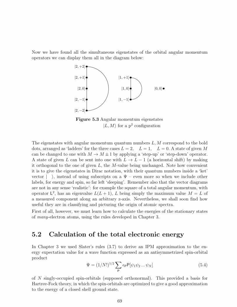
Now we have found all the simultaneous eigenstates of the orbital angular momentumoperators we can display them all in the diagram below:

|2,+2〉•

|2,+1〉•

|2, 0〉•

|2,−1〉•

|2,−2〉•

|1,+1〉•

|1, 0〉•

|1,−1〉•

•|0, 0〉

Figure 5.3 Angular momentum eigenstates

|L,M〉 for a p2 configuration

The eigenstates with angular momentum quantum numbers L,M correspond to the bolddots, arranged as ‘ladders’ for the three cases L = 2, L = 1, L = 0. A state of givenMcan be changed to one with M →M ± 1 by applying a ‘step-up’ or ‘step-down’ operator.A state of given L can be sent into one with L → L − 1 (a horizontal shift) by makingit orthogonal to the one of given L, the M -value being unchanged. Note how convenientit is to give the eigenstates in Dirac notation, with their quantum numbers inside a ‘ket’vector | 〉, instead of using subscripts on a Ψ – even more so when we include otherlabels, for energy and spin, so far left ‘sleeping’. Remember also that the vector diagramsare not in any sense ‘realistic’: for example the square of a total angular momentum, withoperator L2, has an eigenvalue L(L + 1), L being simply the maximum value M = L ofa measured component along an arbitrary z-axis. Nevertheless, we shall soon find howuseful they are in classifying and picturing the origin of atomic spectra.

First of all, however, we must learn how to calculate the energies of the stationary statesof many-electron atoms, using the rules developed in Chapter 3.

5.2 Calculation of the total electronic energy

In Chapter 3 we used Slater’s rules (3.7) to derive an IPM approximation to the en-ergy expectation value for a wave function expressed as an antisymmetrized spin-orbitalproduct

Ψ = (1/N !)1/2∑

P

ǫPP[ψ1ψ2 ... ψN ] (5.4)

of N singly-occupied spin-orbitals (supposed orthonormal). This provided a basis forHartree-Fock theory, in which the spin-orbitals are optimized to give a good approximationto the energy of a closed shell ground state.

69

For the Carbon atom, the basic spin-orbital product for this state would seem to have theexplicit form

ψ1ψ2 ... ψ6 = (1sα)(1sβ)(2sα)(2sβ)(2p+1α)(2p+1β),

but now we have to recognise the degeneracy and the need to couple the angular momentaof the electrons in the p-orbitals. The last section has shown how to do this: we start fromthe ‘top state’, with maximum z-component (Lz = 2, Sz = 1 in atomic units) and set up awhole range of states by applying the shift operators L−, S− to obtain other simultaneouseigenfunctions with lower quantum numbers (see Fig. 5.3).

The ‘top state’, before antisymmetrizing as in (5.4) will now have the associated product

ψ1ψ2 ... ψ6 = (1sα)(1sβ)(2sα)(2sβ)(2p+1α)(2p+1α) (5.5)

and the states with lower values of M have been found in Example 5.3. The next one‘down’ will be derived by antisymmetrizing the product

(1sα)(1sβ)(2sα)(2sβ)[(p0α)(p+1α) + (p+1α)(p0α)]/√2

and this will give a wavefunction Ψ = (1/√2)(Ψ1 +Ψ2), where

Ψ1 =√N !A[(1sα)(1sβ)(2sα)(2sβ)(p0α)(p+1α)]

(5.6)

Ψ2 =√N !A[(1sα)(1sβ)(2sα)(2sβ)(p+1α)(p0α)].

Here, according to (3.4), each of the two terms is a normalized antisymmetrized product ofsix spin-orbitals – but they differ in the choice of the last two. In getting Slater’s rules forfinding the 1- and 2-electron contributions to the expectation value of the Hamiltonianwe considered only the case 〈H〉 = 〈Ψ|H|Ψ〉, where the functions in the ‘bra’ and the‘ket’ were derived from exactly the same spin-orbital product. So we could use them toget the diagonal matrix elements H11 and H22 but not an ‘off-diagonal’ element such asH12 = 〈Ψ1|H|Ψ2〉.Let’s now look at the general spin-orbital product ψ1ψ2 ... ψR ... ψN , using R, S, T, U, ...to label particular factors, and try to get the matrix element 〈Ψ′|H|Ψ〉, in which theantisymmetrized product Ψ′ differs from Ψ by having a spin-orbital ψ′

R in place of ψR

This will be given by an expression similar to (3.7) but the 1-electron part∑

R〈ψR|h|ψR〉will be replaced by the single term 〈ψ′

R|h|ψR〉, while the 2-electron part will be replacedby the single sum

∑

S( 6=R)[〈ψ′RψS|g|ψRψS〉 − 〈ψ′

RψS|g|ψSψR〉].When the spin-orbital products contain two non-matching pairs, ψ′

R 6= ψR and ψ′S 6= ψS,

the 1-electron part will always contain a zero overlap integral 〈ψ′T |ψT 〉 when T = R or

T = S – so no 1-electron term can arise. On the other hand, the 2-electron part will bereplaced by the single term [〈ψ′

Rψ′S|g|ψRψS〉−〈ψ′

Rψ′S|g|ψSψR〉]. (To prove all these results

you should go back to Examples 3.2 and 3.3, noting that except in the cases indicated theproducts of overlap factors will contain zeros.)

We can now collect all the matrix element rules obtained so far, using the antisymmetrizer√N !A as defined in (3.4):

70

Given Ψ =√N !A[ψ1ψ2 ... ψN ],

the diagonal matrix element 〈Ψ|H|Ψ〉 is given by

〈Ψ|H|Ψ〉 =∑R〈ψR|h|ψR〉+ 12

∑′

R,S[〈ψRψS|g|ψRψS〉 − 〈ψRψS|g|ψSψR〉],

but with a single replacement, giving Ψ′ =√N !A[ψ1ψ2 ... ψ

′R .. ψN ],

the off-diagonal matrix element 〈Ψ′|H|Ψ〉 is given by

〈Ψ′|H|Ψ〉 = 〈ψ′R|h|ψR〉+

∑

S( 6=R)[〈ψ′RψS|g|ψRψS〉 − 〈ψ′

RψS|g|ψSψR〉]

and with two replacements, giving Ψ′ =√N !A[ψ1ψ2 ... ψ

′R .. ψ′

S .. ψN ],the off-diagonal matrix element 〈Ψ′|H|Ψ〉 is given by

〈Ψ′|H|Ψ〉 = [〈ψ′Rψ

′S|g|ψRψS〉 − 〈ψ′

Rψ′S|g|ψSψR〉].

(5.7)

Now we know how to get both diagonal and off-diagonal matrix elements of the Hamilto-nian H, between antisymmetrized spin-orbital products, we can calculate the total elec-tronic energies of all the many-electron states belonging to a given configuration. As anexample, let’s find the total electronic energy of the Carbon atom ground state. Exper-imentally, this is known to be triply degenerate, the three states corresponding to theangular momentum eigenstates |L,M〉 with L = 1, M = 0,±1 (see Fig. 5.3).

The ‘top state’ of the three is an eigenstate of orbital angular momentum, ΨL,M , withquantum numbers L = M = 1. It was derived, just after Fig.4.2, by antisymmetrizingthe spin-orbital product

(closed shell)× (1/√2)(p0p+1 − p+1p0)× (spin factor).

Here the closed-shell spin-orbitals are not shown, while p0, p+1 are the orbital eigenstateswith l = 1,m = 0 and l = 1,m = 1, respectively. (Just as the letters s, p, d, f are used todenote 1-electron eigenstates with l=0, 1, 2, 3, the corresponding capital letters are usedto label the many-electron eigenstates with L = 0, 1, 2, 3.) So the degenerate ground stateof Carbon is a ‘P state’ and we ’ll use Ψ(P ) to denote its wave function.

Example 5.2 Total electronic energy of the Carbon ground state

There are two spin-orbital products, to which the six electrons are to be assigned. Here we’ll simplifythings by dealing only with the electrons outside the closed-shell 1s22s2 core, re-labelling them as ‘1’and ‘2’ and taking both to be in α spin states. The corresponding wave function ΨP then arises onantisymmetrizing the function

(1/√2)[p0(r1)p+1(r2)− p+1(r1)p0(r2)]× α(s1)α(s2)

71

– which is a linear combination F = (F1 − F2)/√2 of the two spin-orbital products

F1 = p0(r1)α(s1)p+1(r2)α(s2)

F2 = p+1(r1)α(s1)p0(r2)α(s2).

The resultant 2-electron wave function is thus Ψ(P ) = (Ψ1 − Ψ2)/√2, where the two antisymmetrized

and normalized components are Ψ1 =√2AF1 and Ψ2 =

√2AF2. The energy of the open-shell electrons

in the field of the core will then be

EP = 〈Ψ(P )|H|Ψ(P )〉 = (1/√2)2(H11 +H22 −H12 −H21),

where H11 etc. are matrix elements of the Hamiltonian between the two components of Ψ(P ) and maybe evaluated in terms of the orbital integrals, using the rules (5.7).

Here we’ll simply indicate the evaluation of H11 etc. with the spin-orbitals ψ1 = p0 α and ψ2 = p+1 αused in Ψ1 and Ψ2 :

〈Ψ1|H|Ψ1〉 = 〈ψ1|h|ψ1〉+ 〈ψ2|h|ψ2〉+ 〈ψ1ψ2|g|ψ1ψ2〉 − 〈ψ1ψ2|g|ψ2ψ1〉〈Ψ2|H|Ψ2〉 = 〈ψ2|h|ψ2〉+ 〈ψ1|h|ψ1〉+ 〈ψ2ψ1|g|ψ2ψ1〉 − 〈ψ2ψ1|g|ψ1ψ2〉〈Ψ1|H|Ψ2〉 = 〈ψ1ψ2|g|ψ2ψ1〉 − 〈ψ1ψ2|g|ψ1ψ2〉

When the Hamiltonian contains no spin operators (the usual first approximation) the diagonal 1-electronintegrals each give the energy ǫ2p of a 2p-electron in the field of the 1s22s2 core, but off-diagonal elementsare zero because they are between different eigenstates. The 2-electron terms reduce to ‘Coulomb’ and‘exchange’ integrals, similar to those used in Chapter 3, involving different 2p-orbitals. So it’s a long andcomplicated story, but the rules in (5.7) provide all that’s needed (apart from a bit of patience!).

The Carbon ground state in Example 5.2 is described as 3P (triplet-P) because it has spinquantum number S = 1 and therefore 3 components, with MS = 0, ±1. But it is alsodegenerate owing to the three possible z-components of the orbital angular momentum,with M(L) = 0, ±1, for L = 1. As we shall see shortly, this degeneracy is removed –or ‘broken’ – when small terms are included in the Hamiltonian. First, there is a termdescribing the interaction between the magnetic field arising from orbital motion of theelectron (see Book 10) and the magnetic dipole associated with electron spin. This givesrise to a fine structure of the energy levels, which are separated but remain threefolddegenerate for different values of MS; only when an external magnetic field is applied,to fix a definite axis in space, is this remaining degeneracy broken – an effect called“Zeeman splitting” of the energy levels.

The energy-level structure of the lowest electronic states of the Carbon atom is indi-cated later in Figure 5.4, which shows the positions of the first few levels as determinedexperimentally by Spectroscopy.

There are other states belonging to the electron configuration 2p2, whose energies havenot so far been considered. They are singlet states, labelled in Fig. 5.4 as 1D and 1S; whyhave we not yet found them? The reason is simply that we started the energy calculationusing a wave function with only ‘spin-up’ electrons outside the closed shell 1s22s2 andgot the other functions by applying only the orbital step-down operator L−: this leavesunchanged the spin factor α(s1)α(s2) which represents a triplet state with S = 1. In fact,the Pauli Principle tells us at once that only the 3P state is then physically acceptable: it

72

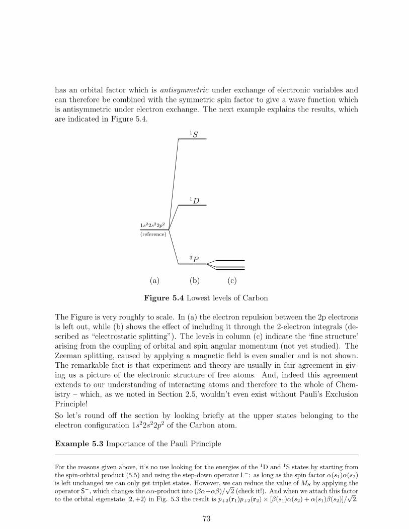
has an orbital factor which is antisymmetric under exchange of electronic variables andcan therefore be combined with the symmetric spin factor to give a wave function whichis antisymmetric under electron exchange. The next example explains the results, whichare indicated in Figure 5.4.

1s22s22p2

(reference)

3P

1D

1S

(a) (b) (c)

Figure 5.4 Lowest levels of Carbon

The Figure is very roughly to scale. In (a) the electron repulsion between the 2p electronsis left out, while (b) shows the effect of including it through the 2-electron integrals (de-scribed as “electrostatic splitting”). The levels in column (c) indicate the ‘fine structure’arising from the coupling of orbital and spin angular momentum (not yet studied). TheZeeman splitting, caused by applying a magnetic field is even smaller and is not shown.The remarkable fact is that experiment and theory are usually in fair agreement in giv-ing us a picture of the electronic structure of free atoms. And, indeed this agreementextends to our understanding of interacting atoms and therefore to the whole of Chem-istry – which, as we noted in Section 2.5, wouldn’t even exist without Pauli’s ExclusionPrinciple!

So let’s round off the section by looking briefly at the upper states belonging to theelectron configuration 1s22s22p2 of the Carbon atom.

Example 5.3 Importance of the Pauli Principle

For the reasons given above, it’s no use looking for the energies of the 1D and 1S states by starting fromthe spin-orbital product (5.5) and using the step-down operator L−: as long as the spin factor α(s1)α(s2)is left unchanged we can only get triplet states. However, we can reduce the value of MS by applying theoperator S−, which changes the αα-product into (βα+αβ)/

√2 (check it!). And when we attach this factor

to the orbital eigenstate |2,+2〉 in Fig. 5.3 the result is p+2(r1)p+2(r2)× [β(s1)α(s2) + α(s1)β(s2)]/√2.

73

This is a linear combination of the two spin-orbital products

F1 = p+1(r1)β(s1)p+1(r2)α(s2)

F2 = p+1(r1)α(s1)p+1(r2)β(s2),

namely F = (F1+F2)/√2; but it still cannot give a wave function that satisfies the Pauli Principle, being

totally symmetric under electron exchange. If we antisymmetrize F it just disappears!

Remember, however, that the step-down operator L− changed the quantum number M in a state |L,M〉but not (see Fig. 5.3) the value of L. To change L we had to find a second combination of the componentstates in |L,M〉, orthogonal to the first. It’s just the same for the spin eigenfunctions; and the orthogonal‘partner’ of (F1 + F2)/

√2 is clearly (F1 − F2)/

√2, which has a singlet spin factor with S =MS = 0.

All we have to do, then, to get the singlet D-states is to use the original orbital eigenfunctions butattaching the spin factor [β(s1)α(s2) − α(s1)β(s2)]/

√2 in place of the triplet factor α(s1)α(s2). As the

five states are degenerate it’s enough to calculate the electronic energy for any one of them e.g. the‘top’ state, with (after antisymmetrizing) the wave function Ψ(L=2;S=0). This is the linear combination

Ψ(D) = (Ψ1 −Ψ2)/√2 of the antisymmetrized products

Ψ1 =√2A[p+1(r1)β(s1)p+1(r2)α(s2)]

Ψ2 =√2A[p+1(r1)α(s1)p+1(r2)β(s2)].

The calculation continues along the lines of Example 5.2: the energy of the open-shell electrons in thefield of the core will now be

ED = 〈Ψ(D)|H|Ψ(D)〉 = (1/√2)2(H11 +H22 −H12 −H21),

where H11 etc. are matrix elements of the Hamiltonian between the two components of Ψ(D) and maybe evaluated in terms of the orbital integrals, using the rules (4.7), just as in the case of Ψ(P ).

A similar calculation can be made for the singlet S state. (Try to do it by yourself!)

You must have been wondering what makes a system ‘jump’ from one quantum stateto another. We met this question even in Book 10 when we were first thinking aboutelectromagnetic radiation and its absorption or emission by a material system; and againin the present Book 11 when we first studied the energy levels of a 1-electron atom and the‘spectral series’ arising from transitions between the corresponding states. The interactionbetween radiation and matter is a very difficult field to study in depth; but it’s time tomake at least a start, using a very simple model.

5.3 Spectroscopy: a bridge between experiment

and theory

Notes to the reader

Before starting this section, you should remind yourself of the electromagnetic spectrum (Section 6.5

of Book 10) and of “Hydrogen – the simplest atom of all” (Chapter 6 of Book 11), where you studied the

energy levels of the H-atom and the series of spectral lines arising from transitions between different

levels. We’re now coming back to the question asked at the end of Chapter 6, namely “What makes

an electron jump?” So you already know what the answer will be: eigenstates of the Hamiltonian are

74

stationary and remain so until you disturb the sytem in some way. Such a disturbance is a perturbation

and depends on the time at which it is applied.

Suppose the system we’re considering has a complete set of stationary-state eigenfunctionsof its Hamiltonian H. As we know from Book 11, these satisfy the Schrodinger equationincluding the time,

HΨ = −~

i

∂Ψ

∂t, (5.8)

even when H itself does not depend on t. The eigenfunctions may thus develop in timethrough a time-dependent phase factor, taking the general form Ψn exp−(i/~)En t,where En is the nth energy eigenvalue. (You can verify that this is a solution of (5.8),provided En satisfies the time-independent equation HΨ = EΨ.)

Now suppose H = H0 + V(t), where V(t) describes a small time-dependent perturba-

tion applied to the ‘unperturbed’ system – whose Hamiltonian we now call H0. And let’sexpand the eigenfunctions of H in terms of those of H0, putting

Ψ(t) =∑

n

cn(t)Ψn exp−(i/~)En t,

where the expansion coefficient cn(t) changes slowly with time (the exponential factorusually oscillates very rapidly). On substituting this ‘trial function’ in (5.8) it followsthat

−~

i

∑

n

(

dcndt− i

~Encn

)

Ψn exp−(i/~)En t =∑

n

HΨn exp−(i/~)En t,

and on taking the scalar product from the left with the eigenvector Ψm we get (only theterm with n = m remains on the left, owing to the factor 〈Ψm|Ψn〉)(

i~dcmdt

+ Emcm

)

exp−(i/~)Em t =∑

n

cn[〈Ψm|H0|Ψn〉+ 〈Ψm|V(t)|Ψn〉] exp−(i/~)En t.

Since the orthonormal set of solutions of the unperturbed equation H0Ψn = EnΨn mustsatisfy 〈Ψm|H0|Ψn〉 = En〈Ψm|Ψn〉 = Enδmn, substitution in the last equation gives (checkit!)

i~dcmdt

=∑

n

cnVmn(t) exp[(i/~)(Em − En)]t, (5.9)

where Vmn(t) is a time-dependent matrix element of the perturbation operator:

Vmn(t) = 〈Ψm|V(t)|Ψn〉.

Now (5.9) is an infinite system of simultaneous equations; and we don’t even know theexact eigenfunctions of H0 – which, to be complete, will include functions forming acontinuum. So it all looks pretty hopeless! The only way forward is to think about veryspecial cases which lead to equations you can solve. That’s what we do next.

75

We start by supposing that the perturbation V depends on time only through being‘switched on’ at time t = t0 and finally ‘switched off’ at a later time t, staying constant,and very small, between the two end points. Note that V may still be an operator (notjust a numerical constant.) If the system is initially known to be in an eigenstate Ψn

with n = i, then the initial values of all cm will be cm(0) = 0 for m 6= i, while ci(0) = 1.

From (5.9), putting all cn’s on the right-hand side equal to zero except the one with n = i,we find a single differential equation to determine the initial rate of change of all cm(t):it will be

i~dcmdt

= Vmi(t) exp (i/~)(Em − Ei)t,

which is a key equation for the first-order change in the coefficients (and means approxi-mating all coefficients on the right in (5.9) by their initial values).

When the operator V is time-independent, the initial value ci(0) = 1 will have changedafter time t to

ci(t) = 1− i

~Vii × t,

while the other coefficients, initially zero, will follow from (5.9) with m 6= i:

cm(t) = − i~

∫ t

0

Vmi(t) exp[(i/~)(Em − Ei)t]dt

= − i~Vmi

[

exp(i/~)(Em − Ei)t

(i/~)(Em − Ei)

]t

0

=Vmi

Em − Ei

[1− exp(i/~)(Em − Ei)t] (5.10)

Now you know (see Book 11, Chapter 3) that |cm(t)|2 will give the probability of observingthe system in state Ψm, with energy Em, at time t after starting in the initial state Ψi att = 0. Thus,

|cm(t)|2 =|Vmi|2

(Em − Ei)2[1− exp(i/~)(Em − Ei)t]× [1 + exp(i/~)(Em − Ei)t]

=|Vmi|2

(Em − Ei)2

(

2 sin(Em − Ei)

2~t

)2

,

where in the second step you had to do a bit of trigonometry (Book 2, Chapter 3).

On setting the energy difference (Em − Ei) = x, this result becomes

P (i→ m) = |cm(t)|2 = 4|Vmi|2x2

(

sint

2~x

)2

(5.11)

and, if you think of this as a function of x, it shows a very sharp peak at x = 0 (whichmeans Em ≈ Ei). The form of the peak is like that shown below in Figure 5.5.

76

By treating x as a continuous variable we can easily get the total probability,∑

m P (i→m), that the system will go into any state close to a final state of ‘given’ energy Ef .For this purpose, we suppose the states are distributed with density ρ(Em) per unit rangearound one with energy Ef . In that case (5.11) will yield a total probability of transitionfrom initial state Ψi to a final state with energy close to Ef , namely

W (i→ f) =∑

m

P (i→ m)→∫

P (i→ m)ρ(Em)dEm.

This quantity can be evaluated by using a definite integral well known to Mathematicians;

∫ +∞

−∞

sin2 αx

x2F (x)dx = παF (0) (5.12)

where F (x) is any ‘well-behaved’ function of x. This means that the “delta function”

δ(0 ; x) = (πα)−1 sin2 αx

x2, (5.13)

when included in the integrand of∫

F (x)dx, simply picks out the value of the functionthat corresponds to x = 0 and cancels the integration. It serves as the kernel of an integraloperator, already defined in Book 11 Section 9, and is a particular representation of theDirac delta function.

On using (5.12) and (5.13), with α = (t/2~), in the expression for W (i→ f), we find (dothe substitution, remembering that x = Em − Ei)

W (i→ f) =

∫

P (i→ m)ρ(Em)δ(0, x)dEm = 4V 2miρ(Em)×

πt

2~=

2πt

~V 2miρ(Ef ) (5.14)

where the delta function ensures that x = Ei−Em = 0 and consequently that transitionsmay occur only when the initial and final states have the same energy, Em ≈ Ef = Ei. Inother words, since Em ≈ Ei the Energy Conservation Principle remains valid in quantumphysics, within the limits implied by the Uncertainty Principle.

For ‘short’ times (still long on an ‘atomic’ scale) this quantity is proportional to t andallows us to define a transition rate, a probability per unit time, as

w(i→ f) = 2π~|Vfi|2ρ(Ef ).

(5.15)

This formula has very many applications in quantum physics and is generally known asFermi’s Golden Rule. In this first application, to a perturbation not depending ontime, the energy of the system is conserved.

77

The form of the transition probability P (i→ f), from which (5.15) was derived, is shownbelow in Figure 5.5 and is indeed ‘sharp’. The half-width of the peak is in fact h/t andthus diminishes with time, being always consistent with what is allowed by Heisenberg’suncertainty principle for the energy of the states.

Figure 5.5 Probability of a transition (see text)

P (i→ f)

Efx = 0(Ef = Ei)

As a second example, let’s think about the absortion and emission of radiation, which lieat the heart of all forms of Spectroscopy. The quanta of energy are carried by photons,but in Book 10 radiation was described in terms of the electromagnetic field in which theelectric and magnetic field vectors, E and B oscillate at a certain frequency, depending onthe type of radiation involved (very low frequency for radio waves, much higher for visiblelight – ranging from red up to blue – and much higher still for X-rays and cosmic rays).That was the ‘classical’ picture of light as a ‘wave motion’. But in quantum physics, a rayof light is pictured as a stream of photons; and much of Book 11 was devoted to getting anunderstanding of this “wave-particle duality”. The picture that finally came out was thata quantum of radiant energy could best be visualized as a highly concentated ‘packet’ ofwaves, sharing the properties of classical fields and quantum particles. (Read Chapter 5of Book 11 again if you’re still mystified!)

So now we’ll try to describe the interaction between an electronic system (consisting of‘real’ particles like electrons and nuclei) and a photon field in which each photon carriesenergy ǫ = hν, where ν is the frequency of the radiation and h isPlanck’s constant. Thisis the ‘semi-classical’ picture, which is completely satisfactory in most applications andallows us to go ahead without needing more difficult books on quantum field theory.

The first step is to think about the effect of an oscillating perturbation of the form

V(t) = Veiωt + V†e−iωt (ω > 0), (5.16)

the operator V being small and time-independent, applied to a system with HamiltonianH0 and eigenstates Ψn exp−(i/~)Ent, with energy En.

78

Transitions may occur, just as they did in the case where there was no oscillating fieldand the frequency-dependent factors were absent. But now there are two terms in theperturbation and each will have its own effect. The argument follows closely the one usedwhen the ω-terms were missing, but the equation for the time-dependent coefficient cm(t)will now be a sum of two parts:

cm(t) = Vmi

[

[1− exp[(i/~)(~ω + Em − Ei)t]

(~ω + Em − Ei)

]

(5.17)

+ V †mi

[

[1− exp[−(i/~)(~ω − Em + Ei)t]

(~ω − Em + Ei)

]

.

On putting ω = 0, the first term reduces to the result given in (5.10), for a single constantperturbation: this was large only when Em ≈ Ei, but now it is large only when Em −Ei + ~ω ≈ 0. The first term can therefore produce a transition from state Ψi to Ψm onlywhen the radiation frequency ν (= ω/2π) is such that ~ω = (h/2π)(2πν) ≈ (Ei − Em).The transition will thus occur only when hν ≈ Ei−Em. This corresponds to emission ofa photon, leaving the system in a state with lower energy Em.

In fact, the transition energy will not be exactly Ei − Em but rather Ei − Ef , where Ef

will be an ‘average’ energy of the group of states into which the emitted electron ‘lands’.The calculation is completed, as in the case of a constant perturbation, by assuming adensity-of-states function ρ(Ef ) for the final state. In the case of emission, the probabilityof a transition into state Ψm at time t will be

P (i→ m) = |cm(t)|2 =|Vmi|2

(hν + Em − Ei)2

(

2 sin(~ω + Em − Ei)

2~t

)2

, (5.18)

which you can get using the same argument that follows equation (5.10). Finally, fol-lowing the same steps (do it!) that led to (5.14) you’ll get the transition rate. Theprobability/unit time for emission of a photon of energy hν (= ~ω)

w(i→ f) = (2π/~)|Vfi|2ρ(Ef )δ(hν + Ef − Ei). (5.19)

The absorption of a photon of energy hν is brought about by the second term in (5.16)and the calculation of the transition rate runs along exactly parallel lines. Thus we find

Emission of a quantum of energy hν :w(i→ f) = (2π/~)|Vfi|2ρ(Ef )δ(hν + Ef − Ei)Absorption of a quantum of energy hν :w(i→ f) = (2π/~)|Vfi|2ρ(Ef )δ(hν − Ef + Ei)

(5.20)

79

As the photon energy is a positive quantity, the final state in absorption will have higher

energy than that in the initial state; and, as you can see, this is nicely taken care of bythe delta-function. In (5.20) the Initial and Final states are labelled ‘i’ and ‘f’ and thedelta-function has the form shown in Figure 5.5. Note that the delta-function peak foremission of a photon is exactly like that shown in the Figure, but the photon-frequencyis given by putting hν + Ef − Ei = 0: this means that hν = Ei − Ef , so the final statehas lower energy than the one the electron comes from; and that corresponds to the peakbeing displaced upwards, from energy Ef ≈ Ei in Figure 5.5 to Ef ≈ Ei − hν in theemission process. In the same way, the absorption of a photon of energy hν would beshown by displacing the peak at energy Ef to one at Ef ≈ Ei + hν.

It may seem that this chapter, with all its difficult theory, has not taken us far beyond theIPM picture we started from – where electrons were supposed independent and assignedto the AOs obtained by solving a 1-electron Schrodinger equation. But in fact we’ve comea very long way: we’re now talking about a real many-electron system (and not only

an atom!) and are already finding how far it’s possible to go from the basic principlesof quantum mechanics (Book 11) towards an understanding of the physical world. Wehaven’t even needed a pocket calculator and we’re already able to explain what goes onin Spectroscopy! Of course, we haven’t been able to fill in all the details – which willdepend on being able to calculate matrix elements like Vif (that require approximatewave functions for initial and final states). But we’ve made a good start.

5.4 First-order response to a perturbation

In Section 5.3 we were dealing with the effect of a small change in the Hamiltonian of asystem, from H0 to H = H0 + V, where the operator V was simply ‘switched on’ at timet = 0 and ‘switched off’ at time t. Now we’ll ask what difference the presence of a time-independent V will make to the eigenstates Ψn of H0, which we’ll call the ‘unperturbed’system. All the states will be stationary states and the time-dependent phase factorsexp−(i/~)Ent may be dropped, having no effect on the expectation values of any time-independent quantities (look back at Section 5.3 of Book 11 if you need to). So we’ll bedealing with the “Schrodinger equation without the time”, HΨ = EΨ.

We’ll also want to get some picture of what the perturbation is doing to the system; andthat will be provided by various density functions, which can show how the electrondistribution is responding. The probability density P (r) – the probability per unit volumeof finding an electron at point r – is well known to you for a 1-electron system, as thesquared modulus |φ(r)|2 of the wave function. But now we need to generalize the idea toa many-electron system – and to include the spin variables s1, s2, ... so we still have workto do.

As in Chapter 1, let’s suppose we have a complete set of functions Φ1,Φ2, ...Φk, ....,in terms of which any wave function of the particle coordinates of the system can be

80

expressed in the form

Ψ(x1,x2, ...xN ) = c1Φ1(x1,x2, ...xN )+c2Φ2(x1,x2, ...xN )+ ...+ckΦk(x1,x2, ...xN )+ ...,(5.21)

where the expansion is, in principle, infinite and the functions of the basis are mostconveniently taken to be normalized and orthogonal: 〈Φj|Φk〉 = δjk. Note that the basisfunctions have now been renamed as Φs (“Phi”s) so as not to mix them up with theeigenfunctions Ψs and remember that xk stands for both position and spin variables(rk, sk).

In Section 1.3 an expansion of this kind was used for 1-electron functions and calleda “linear variation function”. Here, as in dealing with time development of the wavefunction in the last section, the basis used may consist of the energy eigenfunctions of theunperturbed operator H0 (including positive-energy solutions for highly excited states!)We’re not worrying about how difficult it may be to actually set up and calculate withsuch expansions –here it’s enough to use them in building theories!

We know from Section 1.3 that the eigenvalue equation HΨ = EΨ is then equivalent toan (infinite) set of linear equations, Hc = Ec, of which the first three will be

(H11 − E)c1 +H12c2 +H13c3 = 0,

H21c1 + (H22 − E)c2 +H23c3 = 0,

H31c1 +H32c2 + (H33 − E)c3 = 0.

Here, on solving, E will give an upper bound to the lowest energy E1 and c1Ψ1 + c2Ψ2 +c3Ψ3 will give a best approximation to the corresponding wave function Ψ1. The matrixelements Hij = 〈Φi|H|Φj〉 must of course be calculated first and that will define how goodthe approximation can be.

The Perturbation Approach

In perturbation theory the basis functions are usually taken to be eigenfunctions ofthe operator H0 of the unperturbed system, Φk = Ψ0

k, where H0Ψ0k = E0

kΨ0. But here

we’ll keep the Φ-notation for the basis functions, bearing in mind that they may be eitherthe unperturbed eigenfunctions themselves or arbitrary mixtures. In either case, theperturbation of the Hamiltonian will be denoted by H′, so the perturbed system will haveH = H0 + H′. With the first choice, the matrix elements of H will then be simply

Hkj = 〈Φk|H|Φj〉 = E0kδkj +H ′

kj (5.22)

and if we start from the matrix form Hc = Ec it is clear that all the off-diagonal elementsof H will be small, containing only the perturbation operator. As a first approximation,the diagonal part that remains on neglecting them altogether has elements Hkk = E0

k +H ′

kk. In other words, Ek ≈ E0k +H ′

kk and the corresponding matrix eigenvalue equation issatisfied by ck = 1, all other coefficients being zero. This result may be written

δ(1)Ek = H ′kk = 〈Φk|H′|Φk〉,

81

where δ(1)Ek means “first-order change in Ek”. On writing out in full the matrix elementthis becomes

δ(1)Ek =

∫

Φ ∗k (x1,x2, ...xN)H

′Φk(x1,x2, ...xN )dx1dx2 ... dxi ...dxN . (5.23)

This is a very general result. The first-order change in the energy Ek of a state Ψk,produced by a perturbation H′, can be approximated as the expectation value of theperturbation in the unperturbed state Φk. (Here, for simplicity, the state is taken to benon-degenerate.)

How to interpret this result: the electron density function

First we have to think about evaluating the matrix element of H′, the change in theHamiltonian, and that brings us back to the old problem of how to go from one particleto many. We start from the N -electron Hamiltonian H =

∑

i h(i) +12

∑

i,j g(i, j) andadd a perturbation H′. The simplest kind of change is just a change of the field in whichthe electrons move, which changes the potential energy function V (i) for every electroni = 1, 2, ...N . Thus H0 becomes H = H0+H′ with H′ =

∑

i δh(i) =∑

i δV (i), since the KEoperator is not changed in any way. And the matrix element in (5.23) therefore becomes

〈Φk|H′|Φk〉 =

∫

Φ ∗k (x1,x2, ...xN )H

′Φk(x1,x2, ...xN)dx1dx2 ... dxi ...dxN

=

∫

Φ ∗k (x1,x2, ...xN )

∑

i

δV (i)Φk(x1,x2, ...xN)dx1dx2 ... dxi ...dxN .

Remember that a typical integration variable xi really stands for the three componentsof the position vector ri of Electron i, together with its ‘spin variable’ si, so the volumeelement dxi means dridsi. Remember also that

Φ ∗k (x1,x2, ...xN)× Φk(x1,x2, ...xN )dx1dx2 ... dxi ...dxN

gives the probability of finding electrons labelled 1, 2, ...i, ...N simultaneously in thecorresponding volume elements. This is the basic interpretation of the Schrodinger wavefunction (see Book 11 Chapter 3) extended to a system of many particles.

If we had only two particles, described by a wave function Ψ(x1,x2), the probability offinding Electron ‘1’ in volume element dx1, and ‘2’ at the same time in dx2, would beΨ∗(x1,x2)Ψ(x1,x2)dx1dx2, – the probabilities being “per unit volume”. But the proba-bility of finding Electron ‘1’ in dx1 and Electron ‘2’ just anywhere would be obtained bysumming (in this case integrating) over all possible positions of the second ‘box’ dx2 i.e.

dx1

∫

Ψ∗(x1,x2)Ψ(x1,x2)dx2.

Owing to the antisymmetry principle, (2.15) in Chapter 2, the same result would followif we wanted the probability of finding Electron ‘2’ in ‘box’ dx1, and Electron ‘1’ justanywhere. (You can prove this by interchanging 1 and 2 in the wave function and noting that

82

Ψ∗Ψ will be unchanged.) So, with two electrons, the integration only has to be done once – andthe result then multiplied by 2. The probability of finding an electron, no matter which in dx1

can thus be denoted by ρ(x1)dx1, where ρ(x1) = 2∫

Ψ∗(x1,x2)Ψ(x1,x2)dx2 and is called the“one-electron probability density”.

For N electrons a similar result will follow when you think of Electron ‘1’ in ‘box’ dx1 anddon’t care where all the (N − 1) other electrons are: you get the probability of finding it thereby integrating over all positions of the remaining volume elements. And as you’ll get the sameresult for whichever electron you assign to ‘box’ dx1 you can define

ρ(x1) = N

∫

Ψ∗(x1 x2, ...xN )Ψ(x1,x2, ...xN )dx2 ... dxi ...dxN . (5.24)

as the probability per unit volume of finding an electron (no matter which) ‘at’ point x1.

Now we can come back to the Physics. The expectation value of H′ in state Ψ = Φk will be thesum of N identical terms, coming from the 1-electron quantities δV (i). It will thus be

〈Φk|H′|Φk〉 =

∫

Φ ∗k (x1,x2, ...xN )H′Φk(x1,x2, ...xN )dx1dx2 ... dxi ...dxN

= N

∫

Φ ∗k (x1,x2, ...xN )δV (1)Φk(x1,x2, ...xN )dx1dx2 ... dxi ...dxN .

This can be nicely expressed in terms of the 1-electron density defined in (5.24) and gives forthe first-order energy change (5.23)

δ(1)Ek = 〈Φk|H′|Φk〉 =∫

δV (1)ρ(x1)dx1, (5.25)

– all expressed in terms of the space-spin coordinates of a single electron, just as if we weredealing with a one-electron system!

A generalization: the density matrix

Although (5.25) is a very useful result, as you’ll see presently, you may want to know whathappens if H′ =

∑

i δh(i) where δh(i) is a true operator, not just multiplication by a functionδV (i). In that case it seems that the reduction to (5.25) is not possible because the operatorstands between Ψ∗ and Ψ and will work only on the function that stands to its right. In thestep before (5.25) we were able to bring the wave function and its complex conjugate together,to get the probability density, because

Φ ∗k (x1,x2, ...xN )δV (1)Φk(x1,x2, ...xN ) = δV (1)Φk(x1,x2, ...xN )Φ ∗

k (x1,x2, ...xN )

– the order of the factors doesn’t matter when they are just multipliers. But you can’t do thatif δh(1) contains differential operators: ∂/∂z1, for example, will differentiate everything thatstands to its right and contains coordinates of Electron ‘1’. Here we want the operator to workonly on the Ψ factor, which contains x1, and not on Ψ∗. So we have to ‘trick’ the operator bywriting Φ ∗

k (x′1,x2, ...xN ), where x′

1 is a new variable, instead of Φ ∗k (x1,x2, ...xN ), changing it

back to x1 after the operation.

That makes very little difference: the definition of the 1-electron density in (5.24) is replaced bythat of a 1-electron density ‘matrix’, containing the two variables (x1,x

′1):

ρ(x1;x′1) = N

∫

Ψ(x1,x2, ...xN )Ψ∗(x′1 x2, ...xN )dx2 ... dxi ...dxN (5.26)

83

and the expectation value of H′ =∑

i δh(i) is then given by

〈Ψ|H′|Ψ〉 =∫

[δh(1)ρ(x1;x′1)]x′

1=x1

dx1, (5.27)

where the integration is done after applying the operator and identifying the variables. So thegeneralization needed is very easy to make (you’ve done it before in Section 3.5).

As a first application, however, let’s think of applying a uniform electric field to an atom andasking how it will change the energy E of any stationary state Ψ. (We’ll drop the state label kas it’s no longer needed.)

Example 5.5 Application of external field F to an atom

(Note that we’ll be in trouble if we use E for the electric field, as E is used everywhere for energy ; so nowwe’ll change to F when talking about the electric field. You may also need to refer back to Book 10.)

The components Fx, Fy, Fz of the field vector arise as the gradients of an electric potential φ(x, y, z)along the three axes in space,

Fx = −∂φ∂x, Fy = −∂φ

∂y, Fz = −∂φ

∂z

and an obvious solution is φ(x, y, z) = −xFx−yFy−zFz. (Check it by doing the partial differentiations.)

The change in potential energy of an electron (charge −e) at field point (xi, yi, zi), due to the appliedelectric field, is thus δV (i) = e(xiFx + yiFy + ziFz). We can use this in (5.25) to obtain the first-orderchange in energy of the quantum state Ψ = Φk produced by the field:

δ(1)E = e

∫

(xiFx + yiFy + ziFz)ρ(x1)dx1.

Now the integration∫

(.....)dx1 is over both space and spin variables dx1 ≡ dr1ds1, but in this exampleδh contains no spin operators; and even when the wave function contains spin-orbitals, with spin factorsα(si) and β(si), the spin dependence will ‘disappear’ when the spin integrations are done. A ‘spinless’density function can therefore be defined as P (r1) =

∫

ρ(x1)ds1 and the last equation re-written as

δ(1)E =

∫

δV (r1)P (r1)dr1 = e

∫

(xiFx + yiFy + ziFz)P (r1)dr1,

where the spinless density P (r1) depends only on the spatial coordinates of a single point in ‘ordinary’3-space.

Example 5.5 has given a very transparent expression for the first-order energy changethat goes with a modification of the potential field in which the N electrons of a systemmove. If the potential energy of a single electron at point r1 is changed by δV (r1), thefirst-order energy change of the whole electron distribution will be (dropping the label ‘1’on the integration variable)

δ(1)E =

∫

δV (r)P (r)dr (5.28)

– just as if the distribution were a ‘smeared out’ charge, with P (r)dr electrons per unitvolume at point r.

84

This is an example of the Hellman-Feynman theorem which, as we’ll see in the nextchapter, is enormously important in leading to a simple picture of the origin of the forcesthat hold atoms together in molecules. The result is accurate if the wave function isexact or has been obtained by certain types of variational method, but its main valuelies in providing clear pictorial interpretations of difficult theory. It can also lead tosimple expressions for many quantities that are easily measured experimentally. Thus, inExample 5.5,

δ(1)E = e

∫

(xFx + yFy + zFz)P (r)dr

allows us to evaluate the components of the electric moment of a system. In classicalphysics, a charge qi has an electric moment vector defined as “position vector rifrom origin to charge, × charge” with components µx = xiqi, µy = yiqi, µz = ziqi andwhen there are several charges the total electric moment vector will have componentsµx =

∑

i xiqi, etc. The potential energy of that system of charges, in an applied field F,is −µ · F. In quantum physics, the expression given above has exactly this form (checkit out!) provided the electric moment components are calculated as µx =

∫

x(−e)P (r)dretc. and again this confirms the ‘charge cloud’ interpretation, following (5.28), with P (r)electrons/unit volume, each carrying a charge −e.Before going on to calculate the density functions for a few many-electron atoms weconfirm that (5.24) (and with it (5.26)) are correct for any N-electron system and lead tosimple expectation values of 1-electron quantities.

Example 5.6 The 1-electron density matrix

Probability of Electron 1 in volume element dx1 is

dx1

∫

Ψ(x1 x2, ...xN )Ψ∗(x1,x2, ...xN )dx2 ... dxi ...dxN

where the Ψ∗ function has been written on the right, ready for defining the density matrix.

Since the product ΨΨ∗ is invariant against interchange of electrons, the same result would be obtainedfor finding ‘Electron i’ in dx1. With N electrons, the final result for the electron density is thus correctlygiven in (5.24) as the sum of N contributions. The corresponding density matrix follows on changing thevariable x1 in the Ψ∗ factor to x′

1, giving

ρ(x1;x′1) = N

∫

Ψ(x1 x2, ...xN )Ψ∗(x′1,x2, ...xN )dx2 ... dxi ...dxN .

The expectation value of any 1-electron operator sum,∑

i h(i), is thus

〈∑

i

h(i) 〉 =∫

x′

1→x1

[h(1)ρ(x1;x′1)]dx1,

where the prime is removed before doing the integration. We note in passing that this general resultreduces to the one given in (3.7) for an IPM wave function with occupied spin-orbitals ψ1, ψ2, ...ψi, ...ψN .Thus, on putting

ρ(x1;x′1) = ψ1(x1)ψ

∗1(x

′1) + ... + ψN (x1)ψ

∗N (x′

1),

85

the expectation value becomes

〈∑

i

h(i) 〉 = 〈ψ1|h|ψ1〉+ ... + 〈ψN |h|ψN 〉

– exactly as in (3.7).

Example 5.6 has verified the expression for the density function (5.24) and has given itsform in terms of the occupied spin-orbitals in an IPM wave function. Thus

ρ(x1) = ψ1(x1)ψ∗1(x1) + ψ2(x1)ψ

∗2(x1) + ....+ ψN(x1)ψ

∗N(x1) (5.29)

is the 1-electron density function, while

ρ(x1;x′1) = ψ1(x1)ψ

∗1(x

′1) + ψ2(x1)ψ

∗2(x

′1) + ....+ ψN(x1)ψ

∗N(x

′1) (5.30)

is the 1-electron densitymatrix, the two variables corresponding to row and column indicesin a matrix representation of a density operator ρ. The primed and unprimed variablesare shown here in a corresponding ‘standard’ order.

We haven’t forgotten about the spin! If you write x1 = r1 s1 and aren’t interested inwhether the spin is ‘up’ (s = +1

2) or ‘down’ (s = −1

2), then you can ‘sum’ over both

possibilities to obtain a spinless density function P (r1) =∫

ρ(r1, s1ds1. This is the prob-ability/unit volume of finding an electron, of either spin, at point r1 in ordinary 3-space.The terms in (5.29) depend on spin-orbitals ψi(x) = φi(r)θ(s) where the spin factor θmay be α or β; and ρ(x1) may therefore be written as a sum of the form

ρ(x1) = Pα(r1)α(s1)α∗(s1) + Pβ(r1)β(s1)β

∗(s1), (5.31)

in which the α- and β-terms are

Pα(r1) =∑

i (α)

φi(r1)φ∗i (r1), Pβ(r1) =

∑

i (β)

φi(r1)φ∗i (r1). (5.32)

Here the first sum comes from occupied spin-orbitals with α spin factors and the secondfrom those with β factors. The density matrix may clearly be written in a similar form,but with an extra variable coming from the ‘starred’ spin-orbital and carrying the prime.

The results (5.29) – (5.32) all followed from Example 5.6 and the definition

ρ(x;x′) =∑

i

ψi(x)ψ∗i (x

′),

which gave

〈Ψ|∑

i

h(i)|Ψ〉 =∫

[hρ(x; x′)](x′→x)dx.

These are the IPM forms of the 1-electron density functions and their main properties.

86

When electron interaction is admitted we shall need corresponding results for 2-electrondensities: these are derived in the next example.

Example 5.7 The 2-electron density matrix

The derivation follows closely that in Example 5.6: Probability of Electron 1 in dx1 and Electron 2simultaneously in dx2

= dx1dx2

∫

Ψ(x1 x2, ...xN )Ψ∗(x1,x2, ...xN )dx3 ... dxi ...dxN

Here the Ψ∗ function has been written on the right, ready for defining the density matrix, and the first twovolume elements are kept ‘fixed’. Again, Electrons i and j would be found in dx1 and dx2, respectively,with exactly the same probability. But the pair could be chosen from the N electrons in N(N − 1)different ways (with one already chosen there are only N − 1 others to choose from). Adding all theseidentical probabilities means that the total probability of finding any two electrons in dx1 and dx2 willbe

dx1dx2

∫

Ψ(x1 x2, ...xN )Ψ∗(x1,x2, ...xN )dx3 ... dxi ...dxN .

Let’s denote this ‘pair’ probability by dx1dx2π(x1,x2) (π being the Greek letter ‘p’), so that – on droppingthe volume elements – the pair density is π(x1,x2) =

∫

Ψ(x1 x2, ...xN )Ψ∗(x1,x2, ...xN )dx3 ... dxi ...dxN .The corresponding 2-electron density matrix follows when we put primes on the arguments x1 and x2 inthe function Ψ∗ on the right; the result is denoted by π(x1,x2;x

′1,x

′2) and the pair probability results on

identifying the primed and unprimed variables. Thus π(x1,x2) = π(x1,x2;x1,x2).

As in Example 5.6, the 2-electron density matrix for a system with an IPM wave function can be writtendown by inspection of the results obtained in Chapter 3. Thus, from (3.7) the expectation value of theelectron interaction term

∑′(i, j)g(i, j) is given as

〈Ψ|∑′

(i, j)g(i, j)|Ψ〉 =∑

(i,j)

(〈ψiψj |g(1, 2)|ψiψj〉 − 〈ψiψj |g(1, 2)|ψjψi〉)

where g(1, 2) is the 2-electron operator acting on functions of x1 and x2. (Labels are needed to indicatetwo space-spin variables.) Note that the second matrix element has the spin-orbital labels exchanged inthe ket factor, giving the ‘exchange’ term.

The first matrix element can be written

〈ψiψj |g(1, 2)|ψiψj〉 =∫

ψ∗i (x1)ψ

∗j (x2)g(1, 2)ψi(x1)ψj(x2)dx1dx2,

while the second, with a minus sign, is similar but with labels exchanged in the ket factor.

As in the case of the 1-electron densities, we can express this as∫

ψ∗i (x1)ψ

∗j (x2)g(1, 2)ψi(x1)ψj(x2)dx1dx2 =

∫

[g(1, 2)ψi(x1)ψj(x2)ψ∗i (x

′1)ψ

∗j (x

′2)](x′

1→x1,x′

2→x2)dx1dx2

and similarly for the second term.

Now define

π(x1,x2) =∑

(i,j)

(ψi(x1)ψj(x2)ψ∗i (x

′1)ψ

∗j (x

′2)− ψj(x1)ψi(x2)ψ

∗i (x

′1)ψ

∗j (x

′2))

as the 2-electron density matrix. With this definition the many-electron expectation value becomes

〈Ψ|∑′

(i,j)g(i, j)|Ψ〉 =

∫

[g(1, 2)π(x1,x2;x′1,x

′2)](x′

1→x1,x′

2→x2)dx1dx2.

87

and when the operator g(i, j) does not touch the spin variables the integrations over spin can be donefirst:

〈Ψ|∑′

(i,j)g(i, j)|Ψ〉 =

∫

[g(1, 2)Π(r1, r2; r′1, r

′2)](r′1→r1,r′2→r2)dr1dr2,

where the upper-case Greek letter Π is used to denote the spinless 2-electron density matrix. (Remember

that upper-case ”rho”, which is ”P” in the Greek alphabet, was used for the spinless 1-electron density

– that way you won’t get mixed up.)

The conclusions from Examples 5.6 and 5.7 for a state Ψ, represented by a single antisym-metrized spin-orbital product and normalized to unity as in (3.4), are collected below:

Typical terms in the expectation value of the Hamiltonian (3.1) are

〈Ψ|∑i h(i)|Ψ〉 =∑

i〈ψi|h|ψi〉 =∫

[hρ(x;x′)](x′→x)dx,

where the 1-electron density matrix isρ(x;x′) =

∑

i ψi(x)ψ∗i (x

′)

and 〈Ψ|∑′

(i,j)g(i, j)|Ψ〉 =∫

[g(1, 2)π(x1,x2;x′1,x

′2)](x′

1→x1,x′

2→x2)dx1dx2,

where the 2-electron density matrix is

π(x1,x2) =∑

(i,j)(ψi(x1)ψj(x2)ψ∗i (x

′1)ψ

∗j (x

′2)− ψj(x1)ψi(x2)ψ

∗i (x

′1)ψ

∗j (x

′2))

(5.33)

Note that the arguments in the density functions no longer serve to label the electrons– they simply indicate space-spin ‘points’ at which electrons may be found. Now, in thenext Example, we’ll see how things work out in practice.

Example 5.8 Density functions for some atoms

At the beginning of Chapter 5, in Section 5.1, we listed the electron configurations of the first ten atoms ofthe Periodic Table. The first four involved only the two lowest-energy AOs, φ1s and φ2s, which were singlyor doubly occupied by electrons. A doubly occupied orbital appeared once with spin factor α and oncewith spin factor β, describing electrons with ‘up-spin’ and ‘down-spin’, respectively. The correspondingspin-orbitals were denoted by ψ1 = φ1sα, ψ2 = φ1sβ, ψ3 = φ2sα, ψ4 = φ2sβ and, on putting in thespace and spin variables, the spin-orbital φ1s(r)α(s) will describe an electron at point r in 3-space, withspin s. Remember that r = x, y, z (using Cartesian coordinates), while s is a discrete variable with onlytwo values, s = 1

2 for an ‘up-spin’ electron or − 12 for ‘down-spin’. Now we can begin.

The Hydrogen atom (H) has one electron in a doubly degenerate ground state, described by spin-orbitalφ1sα or φ1sβ. The 1-electron density function for the up-spin state will therefore be

ρ(x) = ψ1(x)ψ∗1(x) = φ1s(r)φ

∗1s(r)α(s)α

∗(s)

88

and the 1-electron density matrix will be

ρ(x;x′) = ψ1(x)ψ∗1(x

′) = φ1s(r)φ∗1s(r

′)α(s)α∗(s′).

The ‘spinless’ counterparts of these functions follow, as we guessed in Example 5.5, by integrating over theunwanted variable (in this case spin) after removing the prime. (Remember we always use orthonormalspin functions, so 〈α|α〉 = 1, 〈α|β〉 = 0, etc. Thus we find the spinless density

P (r) =

∫

ρ(x)ds = φ1s(r)φ∗1s(r)

∫

α(s)α∗(s)ds = φ1s(r)φ∗1s(r)

and the spinless density matrix P (r; r′) = φ1s(r)φ∗1s(r

′) – just as if the wave function contained orbitalswith no spin factors.

The Helium atom (He) has a non-degenerate ground state, with two electrons in the 1s AO, but tosatisfy the Pauli principle its wave function must be an antisymmetrized spin-orbital product (3.4) andwe must therefore use (5.29) and (5.30). For the ground state, the results are

ρ(x) = φ1s(r)φ∗1s(r)α(s)α

∗(s) + φ1s(r)φ∗1s(r)β(s)β

∗(s)

and

ρ(x;x′) = φ1s(r)φ∗1s(r

′)α(s)α∗(s′) + φ1s(r)φ∗1s(r

′)β(s)β∗(s′).

The densities of up-spin and down-spin electrons are clearly, from (5.32),

Pα(r) = φ1s(r)φ∗1s(r), Pβ(r) = φ1s(r)φ

∗1s(r)

and the corresponding density matrices are

Pαα(r, r′) = φ1s(r)φ

∗1s(r

′), Pββ(r, r′) = φ1s(r)φ

∗1s(r

′).

The up-spin and down-spin components of the total electron density are equal whenever the spin-orbitalsare doubly occupied: Total density = Pα(r)+Pβ(r). But the difference of the densities is also an importantquantity: it is called the spin density and is usually defined as Q(r) = 1

2 (Pα(r) − Pβ(r)). (The12 is

the spin angular momentum in units of ~, so it is sensible to include it – remembering that the electroncharge density −eP (r) is measured in units of charge, with e = 1.)

The Lithium atom (Li) has a degenerate ground state, the third electron being in the 2s orbital withup-spin or down-spin. The electron density function for the up-spin state follows from (5.29) as

ρ(x) = φ1s(r)φ∗1s(r)α(s)α

∗(s) + φ1s(r)φ∗1s(r)β(s)β

∗(s) + φ2s(r)φ∗2s(r)α(s)α

∗(s).

You can do the rest yourself. The new features of this atom are (i) an inner shell of two electrons, withequal but opposite spins, in a tightly bound 1s orbital, and (ii) a valence shell holding one electron,in a diffuse and more weakly bound 2s orbital, with no other electron of opposite spin. This atom hasa resultant spin density, when in the up-spin state, Q(r) = 1

2φ2s(r)φ∗2s(r) and this ‘free’ spin density,

almost entirely confined to the valence shell, is what gives the system its chemical properties.

Beryllium (Be) is another ‘closed-shell’ system, with only doubly-occupied orbitals, and like Heliumshows little chemical activity.

Boron (B), with one more electron, must start filling the higher- energy p-type AOs such as 2px, 2py, 2pz

and the next few atoms bring in important new ideas.

89

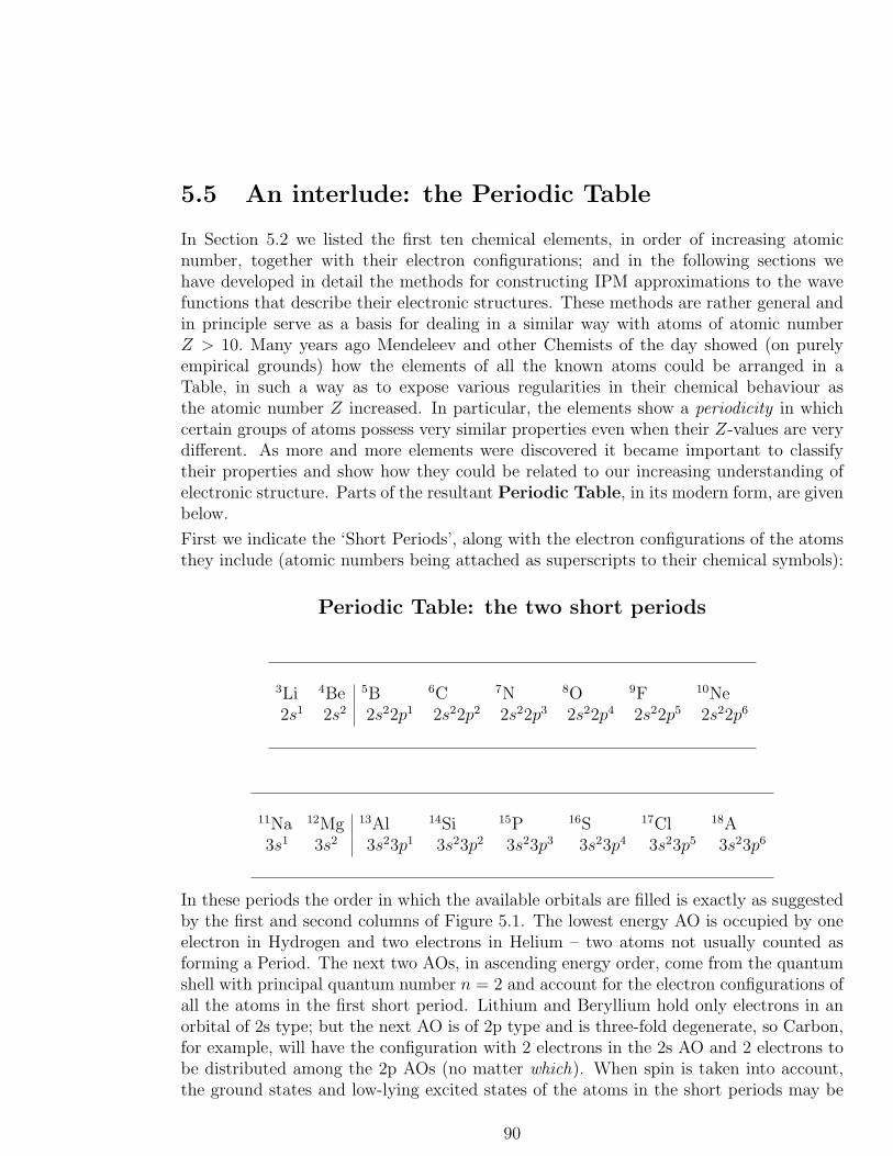
5.5 An interlude: the Periodic Table

In Section 5.2 we listed the first ten chemical elements, in order of increasing atomicnumber, together with their electron configurations; and in the following sections wehave developed in detail the methods for constructing IPM approximations to the wavefunctions that describe their electronic structures. These methods are rather general andin principle serve as a basis for dealing in a similar way with atoms of atomic numberZ > 10. Many years ago Mendeleev and other Chemists of the day showed (on purelyempirical grounds) how the elements of all the known atoms could be arranged in aTable, in such a way as to expose various regularities in their chemical behaviour asthe atomic number Z increased. In particular, the elements show a periodicity in whichcertain groups of atoms possess very similar properties even when their Z-values are verydifferent. As more and more elements were discovered it became important to classifytheir properties and show how they could be related to our increasing understanding ofelectronic structure. Parts of the resultant Periodic Table, in its modern form, are givenbelow.

First we indicate the ‘Short Periods’, along with the electron configurations of the atomsthey include (atomic numbers being attached as superscripts to their chemical symbols):

Periodic Table: the two short periods

3Li 4Be 5B 6C 7N 8O 9F 10Ne2s1 2s2 2s22p1 2s22p2 2s22p3 2s22p4 2s22p5 2s22p6

11Na 12Mg 13Al 14Si 15P 16S 17Cl 18A3s1 3s2 3s23p1 3s23p2 3s23p3 3s23p4 3s23p5 3s23p6

In these periods the order in which the available orbitals are filled is exactly as suggestedby the first and second columns of Figure 5.1. The lowest energy AO is occupied by oneelectron in Hydrogen and two electrons in Helium – two atoms not usually counted asforming a Period. The next two AOs, in ascending energy order, come from the quantumshell with principal quantum number n = 2 and account for the electron configurations ofall the atoms in the first short period. Lithium and Beryllium hold only electrons in anorbital of 2s type; but the next AO is of 2p type and is three-fold degenerate, so Carbon,for example, will have the configuration with 2 electrons in the 2s AO and 2 electrons tobe distributed among the 2p AOs (no matter which). When spin is taken into account,the ground states and low-lying excited states of the atoms in the short periods may be

90

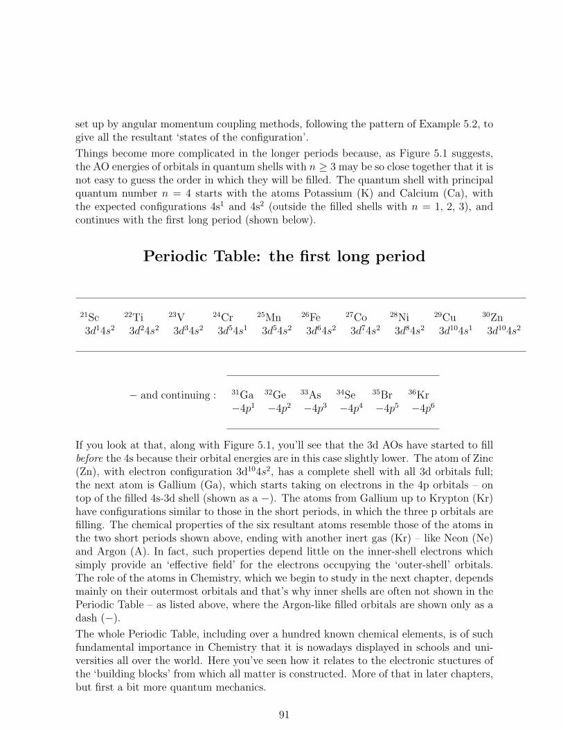
set up by angular momentum coupling methods, following the pattern of Example 5.2, togive all the resultant ‘states of the configuration’.

Things become more complicated in the longer periods because, as Figure 5.1 suggests,the AO energies of orbitals in quantum shells with n ≥ 3 may be so close together that it isnot easy to guess the order in which they will be filled. The quantum shell with principalquantum number n = 4 starts with the atoms Potassium (K) and Calcium (Ca), withthe expected configurations 4s1 and 4s2 (outside the filled shells with n = 1, 2, 3), andcontinues with the first long period (shown below).

Periodic Table: the first long period

21Sc 22Ti 23V 24Cr 25Mn 26Fe 27Co 28Ni 29Cu 30Zn3d14s2 3d24s2 3d34s2 3d54s1 3d54s2 3d64s2 3d74s2 3d84s2 3d104s1 3d104s2

− and continuing : 31Ga 32Ge 33As 34Se 35Br 36Kr−4p1 −4p2 −4p3 −4p4 −4p5 −4p6

If you look at that, along with Figure 5.1, you’ll see that the 3d AOs have started to fillbefore the 4s because their orbital energies are in this case slightly lower. The atom of Zinc(Zn), with electron configuration 3d104s2, has a complete shell with all 3d orbitals full;the next atom is Gallium (Ga), which starts taking on electrons in the 4p orbitals – ontop of the filled 4s-3d shell (shown as a −). The atoms from Gallium up to Krypton (Kr)have configurations similar to those in the short periods, in which the three p orbitals arefilling. The chemical properties of the six resultant atoms resemble those of the atoms inthe two short periods shown above, ending with another inert gas (Kr) – like Neon (Ne)and Argon (A). In fact, such properties depend little on the inner-shell electrons whichsimply provide an ‘effective field’ for the electrons occupying the ‘outer-shell’ orbitals.The role of the atoms in Chemistry, which we begin to study in the next chapter, dependsmainly on their outermost orbitals and that’s why inner shells are often not shown in thePeriodic Table – as listed above, where the Argon-like filled orbitals are shown only as adash (−).The whole Periodic Table, including over a hundred known chemical elements, is of suchfundamental importance in Chemistry that it is nowadays displayed in schools and uni-versities all over the world. Here you’ve seen how it relates to the electronic stuctures ofthe ‘building blocks’ from which all matter is constructed. More of that in later chapters,but first a bit more quantum mechanics.

91

5.6 Effect of small terms in the Hamiltonian

Most atoms do not have closed-shell ground states and, as we saw in the last section, thatmakes them much more interesting. In particular, electron configurations with degenerateAOs that are incompletely filled can show a rich variety of electronic states. Even whenthe separation of atomic energy levels is very small it is easy to observe experimentallywith present-day techniques: these usually require the application of strong magneticfields which allow one to ‘see’ the effects of coupling between the applied field and anyfree spins – which carry magnetic dipoles (see Book 10). The spin-field (Zeeman)interaction gives rise to a perturbation of the form

H′Z = gβ

∑

i

B · S(i), (5.34)

where β = e~/2m is called the “Bohr magneton” (don’t confuse it with a spin eigenstate),B is the flux density of the magnetic field, and g is a number very close to 2 (whichindicates that spin is twice as effective as orbital motion of a charge in producing amagnetic dipole).

The ‘normal’ interaction between the field and an electron with orbital angular momentumL(i) gives a perturbation

H′mag = β

∑

i

B · L(i), (5.35)

which represents a classical field-dipole interaction). In both cases the summation is overall electrons.

There are many other interaction terms, which you don’t even need to know about, butfor a free atom there are some simplifications and it’s fairly easy to see how the finestructure of the energy levels can arise and how the states can be classified. So we’ll endthis chapter by using what we already know about spin and orbital angular momenta. Theunperturbed states of a Carbon 2p2 configuration, with energy levels represented in Figure5.4, were constructed as linear combinations of antisymmetrized products of spin-orbitalsso as to be simultaneous eigenstates of the commuting operators H, L2, Lz, S

2, Sz (all inIPM approximation). But the fine structure of the triplet P level, indicated in Column(c), was not accounted for – though it was put down to “spin-orbit coupling”, which couldbe admitted as a perturbation. Classically, the interaction energy between two magneticdipolesm1,m2 is usually taken to be proportional to their scalar productm1 ·m2, so it willbe no surprise to find that in quantum mechanics the spin-orbit perturbation operator,arising from the spin dipole and the orbital dipole, takes the approximate form (mainterm only)

H′SL(i) =

∑

i

f(ri)S(i) · L(i), (5.36)

where the factor f(ri) depends on distance ri of Electron i from the nucleus, but is alsoproportional to nuclear charge Z and therefore important for heavy atoms.

92

To understand the effect of such terms on the levels shown in Fig. 5.4, we remember thateigenstates of the operators L2, Lz and S2, Sz can be coupled to give eigenstates of totalangular momentum, represented by the operators Jx, Jy, Jz, defined as

Jx = Lx + Sx, Jy = Ly + Sy, Jz = Lz + Sz,

and that these operators have exactly the same commutation properties as all angularmomentum operators (reviewed in Section 5.1). Thus, it should be possible to find simul-taneous eigenstates of the operators J2 = J2x + J2y + J2z, and Jz, with quantum numbers(J,MJ), and also the shift operators J+ = Jx + iJy and J− = Jx − iJy. To check thatthis really is possible, let’s start from the orbital and spin eigenstates (already found)with quantum numbers (L,ML) and (S,MS), calling them ΦL,ML

and ΘS,MS, respectively.

The product of the ‘top’ states, with ML = L and MS = S, is clearly an eigenstate ofJz = Lz+Sz because each operator works only on ‘its own’ eigenfunction (orbital or spin),giving Jz(ΦL,ML=LΘS,MS=S) = L+S(ΦL,ML=LΘS,MS=S), and this means the product func-tion is an eigenfunction of Jz with the maximum available quantum number MJ = L+S,which implies that J = L + S is the quantum number for the corresponding eigenstateof J2. This really is the top state because it can’t be stepped up (J+ = L+ + S+ and theproduct will be annihilated by one or other of the two operators). On the other hand,(ΦL,LΘS,S) can be stepped down by using (J− = L− + S−). This will give a functionwith L and S unchanged, which is a combination of ΦL,L−1ΘS,S and ΦL,LΘS,S−1 with Junchanged but MJ reduced by 1.

You’ve done all this before! There will be another combination, orthogonal to the firstand still with the Jz quantum number reduced to MJ − 1, and this must be the top stateof a new series with J = L + S − 1. If you do the same operations all over again youcan reduce the MJ -value to L + S − 2 and then, by finding an orthogonal combination,arrive at the top state of a new series with J = MJ = L + S − 2. As you can see, thisgets terribly tedious. But it can be done and the conclusion is easy enough to visualize:you add vectors by adding their corresponding components. In adding orbital and spinangular momentum vectors you start with the vectors ‘in line’, so J = MJ = ML +MS,only the quantized z-components being significant; and then you step down by using theJ− operator to get all the 2J + 1 states of the series with the same J = M + S. Thenyou move to the series with J =M + S − 1 and MJ going down from J to −J in integersteps, corresponding to the allowed projections of an arrow of length J on the z-axis. Bycarrying on in that way you find all the vector-coupled states with

J = L+ S, L+ S − 1, L+ S − 2, ...., |L− S|.

Since J is a positive number the process must stop when the next step would violate thiscondition; that’s why the last state has a J value which is the magnitude of the differencein lengths of the L- and S-vectors.

We can now come back to Figure 5.4 and the splitting of the energy levels in Column(c). In principle we could estimate the effect of the perturbation terms (5.34), (5.35) and(5.36) by getting their matrix elements relative to the unperturbed functions and then

93

solving a system of secular equations, along the lines of Section 5.4; but it’s much nicer, ifyou don’t want any numerical detail, to use the fact that the 2L+1 orbital eigenstates ofL2 and the 2S + 1 spin eigenstates of S2 may in general be mixed by the perturbation toproduce eigenstates of the operators J2 and Jz, which also commute with the Hamiltonian.We’ve just found how the vector-coupled states that result can be labelled in terms of theeigenvalues J and MJ ; and we know that states with different sets of eigenvalues will ingeneral have different energies.

The levels in Figure 5.4 result from the unperturbed 2-electron states with quantumnumbers L = 1,ML = 1, 0, −1 and S = 1,MS = 1, 0, −1 and for each choice of L andS we can obtain all the allowed spin-coupled states of given J and MJ . Moreover, theunperturbed states have been constructed from antisymmetrized spin-orbital productsand the Pauli Principle is thus taken care of from the start. Let’s take the possible statesone at a time:

L = 2, S = 1

In Example 5.3 this case was ruled out, being completely symmetric under electron ex-change, so J = L+ S = 3 is excluded. But with S = 0 we pass to the next

L = 2 S = 0 J = 2

L = 2 means this is a D state (2 units of orbital angular momentum) and S = 0 meansthis is a spin singlet, so the full state label is 1D as shown in Fig.5.4

L = 1 S = 1 J = 2

L = 1 means this is a P state (1 unit of orbital angular momentum) and S = 1 meansthis is a spin tripet, so the full state label is 3P as shown in Fig. 5.4 with some finestructure resulting from spin-orbit coupling. When J = 2 there are 2J + 1 = 5 statesof different MJ : these are the Zeeman states, which are degenerate in the absence of anexternal magnetic field. But the top state (J = MJ = 2) can be stepped down to give aseries with J = 1, still 3P states, J being J = L+ S − 1 with L = 1 and S = 1. Anotherstep down gives J = L+ S − 2 = 0, a single state with the L- and S-vectors anti-parallelcoupled. To label these component states, of which there are 9 (=5+3+1), it is usual toadd a subscript to the ‘term symbols’ shown in Fig. 5.4, giving the value of J. The statesof the 3P multiplet are then labelled 3P2,

3P1,3P0, in descending order of energy. The

highest-energy state of the multiplet is the one in which the magnetic dipoles point in thesame direction; the lowest is that in which their arrows are opposed – just as in ClassicalPhysics.

Of course, we’re still using an IPM picture, which is only a poor approximation, butit’s amazing how much understanding we can get from it – even without any numericalcalculations. The tiny shifts of the energy levels, brought about by the small terms in theHamiltonian, are described as “fine structure”. When observed spectroscopically theygive important information about the electronic structure of the atoms: first of all theytell us what atom we are looking at (no two atoms give exactly the same ‘finger prints’)and secondly they tell us whether or not there are singly occupied orbitals, containingun-paired spins that are free to couple with the spins of other atoms. So they are useful

94

for both chemical analysis and for understanding chemical reactivity – so much sothat most of our big hospitals have expensive equipment for detecting the presence ofunpaired spins in the atoms of the cells in our bodies!

95

Chapter 6

Molecules: first steps –

6.1 When did molecules first start to form?

You first started learning about how atoms could combine, to form molecules, in Chapter1 of Book 5. Since then, in Book 6, you’ve learnt more about matter in general and thehistory of our planet Earth as a member of the Solar System. You must have been struckby the time-scale on which things happen and the traces they leave behind in the rocks,like the fossil remains of creatures that lived here many millions of years ago. And inBooks 7-9 you learnt about the evolution of all those creatures (including ourselves!),starting from the earliest and simplest forms of life. Before studying molecules in moredetail you may be wondering where the atoms themselves came from; and that takes usback to the beginning of the Universe. We’ll have to tell the story in the light of what weknow now (or at least think we know, on the basis of all the evidence we have).

About 14 billion years ago, all the particles in the present Universe were very close togetherin a ‘ball’ of unbelievably dense matter. This ball exploded as a result of the interactionsthat drove the particles apart: we now call that event the Big Bang. The particlesspread out in empty space, at great speed, to form an Expanding Universe which isstill getting bigger and bigger. As they interacted, the particles eventually began to formatoms – first of all those of Hydrogen, the lightest known atom, consisting of one protonand one electron. So at one stage the Universe could be pictured as a dense cloud ofHydrogen. But it didn’t stay that way.

What happened in the early Universe?

The atomic nuclei (protons) could also come together in pairs to form new nuclei, thoseof the Helium ion He2+ (the 2+ indicating that the neutral Helium atom has lost twoelectrons to give a bare nucleus with two units of positive charge). This process is callednuclear fusion and was first mentioned in Book 4 Section 8.3 (which you should readagain before going on). When two protons fuse in this way the total mass of the systemis reduced by a factor of about 0.7×10−2 and since a proton has a mass ≈ 1.66×10−27 kgthe mass lost will be ≈ (0.7× 10−2)(1.66× 10−27 kg) = 2.324× 10−29 kg

96

Now in Section 8.3 of Book 4, you learnt that mass is a form of energy and that the twothings are related by Einstein’s famous formula E = mc2, where c is the speed with whichlight travels (≈ 3× 108ms−1). The mass lost when two protons fuse is thus equivalent toan energy

E = mc2 = (2.324× 10−29 kg)× (9× 1016 m2s−2) = (20.916× 10−13) kgm2 s−2.

But the energy unit here is the Joule: 1 J = 1 kgm2 s−2. That may not seem much, butif you remember that the ‘chemical’ unit of quantity is the ‘mole’ this must be multipliedby the Avogadro number L, the number of systems it contains. The fusion energy of 1mole of proton pairs thus comes out as

(0.602× 1024)× (20.916× 10−13) J = 12.59× 1011 J = 12.59× 108 kJ.

Let’s compare that with the energy released in burning 1 mole of hydrogen gas (oftenused as a rocket fuel). In that case (read section 3.2 of Book 5) the reactants are 1 moleof hydrogen molecules (H2) plus 1 mole of Oxygen molecules (O2); and the products

are 1 mole of water molecules (H2O). The energy change when the reactants go to theproducts is ∆H = HP−HR, where H stands for “Heat content per mole”. On putting inthe experimental values of these quantities for Hydrogen, Oxygen and Water, the result is−571.6 kJ, the minus sign meaning that the total heat content goes down and the energyreleased by burning 1 mole of Hydrogen is 571.6 kJ.

That should be compared with the energy released in the fusion of 1 mole of proton pairs,which we found to be 1.259×109 kJ – over a thousand million kJ. So in the early Universethere was no shortage of energy; its gaseous contents must have existed at an unbelievablyhigh temperature!

What happened in the very early stages?

At the beginning of the first 10 billion years after the Big Bang, as it began to cool,the Universe contained a ‘mish-mash’ of particles with strange names like ‘quarks’ and‘gluons’ (given to them by the people who discovered them), forming a continuous ‘sea’called a plasma. That phase lasted only up to about one second after the BB and wasfollowed by the appearance of heavier particles, mainly protons, electrons and neutrons –collectively known as ‘baryons’ – composed of quarks ‘glued together’ by the gluons.(It’s almost impossible to observe the quarks and gluons because if ever they get out of a baryon theyhave a vanishingly short lifetime and seem to just disappear – until recently nobody knew that a protonwas composed of three quarks, held together by gluons! To find what was inside a proton or a neutronyou had to smash it open by firing other particles at it and observing what came out; and to give these‘projectiles’ enough energy to do that they had to be accelerated to speeds close to that of light. Particle

accelerators are nowadays being built, at great expense, to do that job.)

Then, between about 3 and 20 mins after the BB, when the temperature and density ofthe plasma had fallen to a low enough level, the baryons started coming together to formother nuclei, such as He2+, by the fusion reaction described above.

Much later, between about 200 and 400 thousand years after BB, the positively chargednuclei began to capture electrons from the plasma to form stable neutral particles, mainly

97

neutrons, H-atoms and He-atoms together with a few of the other light atoms, like Carbon,that you’ve already met. These are the atoms needed in building simple molecules, whichwe’ll study in detail in the rest of this chapter. (You might like to read a preview of themin Book 5.)

From that point on there followed a long period, still going on, of ‘structure formation’.First the atoms came together in small groups, which attracted other groups and becamemuch bigger (think of a snowball rolling down a hill and picking up more snow on theway until it becomes a giant snowball): after billions of years these gigantic structuresbecame the first stars; and started coming together in ‘star-clusters’ or ‘galaxies’. Thegalaxy we see in the night sky and call the “Milky Way” was formed in this way between7 and 10 billion years ago and one of the stars in this galaxy is our Sun. The whole SolarSystem, the Sun and the Planets that move in orbits around it, came into existence about8 or 9 billion years after the Big Bang; so planet Earth, the part of the Universe we feelwe know best, is about 41

2billion years old!

But how do we know all that?

We see the stars in the night sky because they shine: they emit radiation in the formof photons, which travel through space at the enormous speed of ≈ 3× 108ms−1 (threehundred million metres per second!) and the light we observe using ordinary (‘optical’)telescopes consists only of photons in a very narrow range of frequencies (as you’ll remem-ber from Book 10, Section 6.5). Most of the light that reaches us is ‘invisible’ but it canall be ‘seen’ by the instruments available to us nowadays – and it all carries informationabout where it came from. We also have radio telescopes, for example, that pick upthe radiation from distant stars. All this radiation can be analised by spectrometers,which give detailed information about the electronic origins of the light they take in (asyou learnt in Section 5.3 of the present Book 12).

If you really think about all this you’ll come to some amazing conclusions. First of allthe distances between stars are so large that it’s most convenient to measure them in‘light years’; 1 light year is the distance travelled by a photon in 1 year and is about9.5×1012km. The nearest stars to our own Sun are about 4 light years away; so the lightthat we see coming from them started in processes that happened 4 years ago. But moredistant stars in the Milky Way galaxy were formed as long as 13 billion years ago andany radiation that comes from them must therefore have been on the way for no less thanabout 13 billion years.

The light that reaches us here on the Earth, from the Milky Way, is very dim and itsspectrum is ‘foggy’ showing little sign of the sharp lines found in atomic spectra observedin the laboratory. But against this background there is always one extremely faint lineat a wavelength of 21.106 cm in the microwave region of the spectrum. Where could itcome from?

When the first atoms began to form, so long ago, they were almost exclusively Hydrogen(one proton plus one electron). And, as you know from Section 5.3, when one of themmakes a transition from one electronic state to another, of lower energy, a photon offrequency ν is emitted with hν = Einitial − Efinal. The lowest electronic state is a 2S

98

doublet, the two 1s levels differing in spin (±12), but now we must remember that the

proton is also a spin-12particle and that the two spins (S = 1

2for the electron and I = 1

2

for the proton) can couple to give a total spin angular momentum with quantum numberF , say, with possible values F = 1

2+ 1

2= 1 and F = 1

2− 1

2= 0. As a result of this nuclear

hyperfine coupling the lowest energy level of the H-atom becomes a doublet with aminute energy separation, confirmed here and now in the laboratory, of 5.874 ×10−6 eV.This is the energy of a quantum of radiation of wavelength 21.106 cm.

What does all this mean? When we say “here and now” we mean “here on Earth” and“now at the time of making the experimental measurement”. But the event we were talk-ing about – the emission of a photon from an atom in a distant part of the Universe – tookplace about 13 billion light years away, which means 13 billion years before our laboratoryexperiments! The predicted energy separation comes from calculations that depend on allthe laws of ‘everyday’ Physics (from Classical Mechanics (Book 4) to Electromagnetism(Book 10) and Quantum Mechanics (Book 11) – as long as extremely high energies orrelativistic velocities are not involved. We can hardly escape the remarkable conclusionthat

The Laws of Physics are invariant against changes of position or

time of the system to which they are applied; and that must have

been true for at least 13 billion years.

Many details remain to be filled in: for example, theory shows that the 21 cm transition isin fact ‘forbidden’ and would probably take place not more than once in 10 million years!But the number of H atoms in the Milky Way is so enormous that the total probabilityof a transition is enough to account for the observed spectral line.

In summary: the fundamental laws of physics are OK and any variations in the behaviourof matter are normally due to changes in external conditions such as temperature anddensity (which may both reach unimaginable values). Now we’re all set to start thinkingabout the next step in the evolution of the Universe: what makes the atoms stick togetherto form molecules?

6.2 The first diatomic systems

As you’ve learnt from Section 6.1, the early Universe once consisted of a hot plasma ofelectrons, neutrons, and protons (H+) that had not yet picked up electrons to becomeneutral Hydrogen atoms (H) – together with a trace of Helium nuclei (He2+) alreadyformed by proton fusion.

Let’s imagine what can happen when a proton meets a Hydrogen atom. There willthen be a composite system, with two protons sharing one electron, namely a hydrogen

molecule ion.

As usual we apply quantum mechanics to this system by first of all setting up the Hamil-tonian operator. We should really suppose all three particles are moving, but we’ll use

99

an approximation that allows for the fact that a proton has a mass almost 2000 timesthat of an electron. The rapidly moving electron then ‘sees’ the nuclei at any instant asif they were at rest in fixed positions. The three-body problem then becomes in effect aone-electron problem with Hamiltonian

h = −12∇2 −

(

1ra

+ 1rb

)

, (6.1)

where ra and rb denote distances of the electron from nuclei ‘a’ and ‘b’ and atomic unitsare used throughout. The ∇2-operator works on the electronic coordinates, to be denotedby r, and will have a form depending on the coordinate system chosen. The energy levelsof the electron are then found by solving the eigenvalue equation

hφ = ǫφ. (6.2)

The energy of the whole system in this ‘fixed nucleus’ approximation will then be

E = 1/Rab + ǫ, (6.3)

where ǫ denotes the electronic energy eigenvalue and Rab is the internuclear distance.(Note that in atomic units the proton charges are Za = Zb = 1 and that the first termin E is their classical Coulomb repulsion energy.) This procedure is called the Born-

Oppenheimer separation of electronic and nuclear motion. Heavy particles (like nuclei)move in good approximation according to classical physics with E, calculated in this way,serving as a potential energy function.

But then we meet the next big problem. For an atom we had ‘ready-made’ atomic orbitals,with the well-known forms (1s, 2s, 2p, 3s, 3p, 3d, etc.) first discussed in Book 11, buthere we know nothing about the forms of the molecular orbitals that will be neededin building corresponding approximations to the molecular wave functions. First of all,then, we need to find how to describe the one-electron system that remains when theelectron is taken away. This system is experimentally well-known: it is the Hydrogenmolecule ion, H+

2 .

How can we get a reasonable first approximation to the lowest-energy molecular orbital(MO)? When the electron is close to Nucleus a, the term 1/ra will be so big that 1/rbmay be neglected in (6.1). The MO will then ‘shrink’ into an atomic orbital (AO) for asingle hydrogen atom. We’ll denote this AO by χa(r), as we’re going to use AOs as basisfunctions out of which more general wave functions, such as MOs, can be constructed.In this process a general MO, call it φ, must change according to φ(r) → caχa(r), sincethis will satisfy the same single-atom eigenvalue equation for any value of a numericalfactor c. Similarly, when r is close to the second nucleus φ(r) will approach a numericalmultiple of the AO χb(r). It follows that an electron in the field of both nuclei may befairly well represented by an MO of the form

φ(r) = caχa(r) + cbχb(r) (6.4)

100

where the constants ca, cb are still to be chosen (e.g. by taking them as variable parametersand using the variation method of Section 1.3) to find the MO of minimum energy. Thisshould give at least a rough description of the ground state.

In fact, however, no calculation is needed because the molecule ion is symmetrical acrossa plane perpendicular to the molecular axis, cutting the system into two equal halves.There is no reason to expect the electron to be found with different probability on thetwo sides of the symmetry plane and this implies that the values of the coefficients ca, cbcan differ, at most, in sign: cb = ±ca. Two acceptable approximate MOs are thus, puttingcb = ca = NB in one MO and cb = −ca = NA in the other

φB(r) = NB[χa(r) + χb(r)], φA(r) = NA[χa(r)− χb(r)]. (6.5)

This case arises only for homonuclear diatomic molecules – in which the two nuclei areidentical. It is important because very many common diatomic molecules, such as H2,N2, O2, are of this type.

The solutions just found are typical Bonding and Antibonding MOs; so called forreasons that will soon become clear. The constantsNA, NB are normalizing factors, chosento give unit probability of finding the electron somewhere in space. For normalization werequire

N 2B〈φB|φB〉 = N 2

B(2 + 2Sab) = 1,

where Sab = 〈χa|χb〉 is the overlap integral between the two AOs. In this way we findMOs

φB(r) =χa(r) + χb(r)√

2 + 2Sab

(6.6)

for the Bonding MO, and

φA(r) =χa(r)− χb(r)√

2− 2Sab

(6.7)

for the Antibonding MO. The following Figure 6.1 gives a very schematic picture of thetwo MOs.

Rab

nodal

plane

Rab+ + + −

Bonding MO Antibonding MO

Figure 6.1 Schematic representation of the two lowest-energy MOs for H+2 .

101

Here, for the ion, H = h, the 1-electron Hamiltonian, and the distinct quantities to becalculated are (using a common notation and supposing the AOs are normalized)

αa = 〈χa|h|χa〉, βab = 〈χa|h|χb〉, αb = 〈χb|h|χb〉, Sab = 〈χa|χb〉. (6.8)

As in Section 1.3 of Chapter 1, the conditions for a stationary value then reduce to

(αa − E)ca = −(βab − ESab)cb

(βab − ESab)ca = −(αb − E)cb.

But when the system is symmetrical, as already noted, we know that cb = ±ca and in thatcase just one equation is enough to give us both eigenvalues. Thus, putting αa = αb = αand choosing cb = ca, the first equation reduces to (α + β) − E(1 + S) = 0; while onchoosing cb = −ca it reduces to (α− β)− E(1−S) = 0. The approximate energies of thetwo states φB(r), φA(r), may then be written

EB =α + β

1 + S=α(1 + S) + β − αS

1 + S, EA =

α− β1− S =

α(1− S)− β + αS

1− S ,

where the numerators have been re-arranged so as to ‘separate out’ the leading terms. Inthis way we find

EB = α +β − αS1 + S

, EA = α− β − αS1− S . (6.9)

Since α is the energy expectation value of an electron very close to one nucleus aloneand (like β) has a negative value, it follows that the Bonding MO φB has a lower energy(EB) than the free- atom AO, while the Antibonding MO φA has a higher energy (EA).Note, however, that the upward displacement of the free-atom energy level in going tothe antibonding level is greater than the downward dispacement in going to the bondinglevel, owing to the overlap term. All this is shown very nicely in a correlation diagram

which shows how the energies of the AOs on two identical atoms are related to those ofthe MOs which result when the atoms are combined to form a homonuclear diatomic

molecule – a ‘homonuclear diatomic’, for short.

Such a diagram, describing the formation of H2, is shown in Figure 6.2, energy levels forthe separate atoms being indicated on the left and right with the MO energies in thecentre.

Figure 6.2 Energies of orbitalsin a homonuclear diatomic.

AO levels shown left and rightMO levels shown in the centre.

102

Remember that we’re still talking about a one-electron system, the hydrogen moleculepositive ion, and that this is homonuclear. But before going to the neutral molecule, withtwo electrons, we may want to think also about other 2-electron systems such as HeH+,with one of the Hydrogens (H) replaced by a Helium atom (He) and one of the threeelectrons taken away – giving you the Helium Hydride positive ion. In that case we’llhave a heteronuclear system in which the two nuclei are different and the forms of theacceptable MOs must also be changed. Helium hydride is a very rare species, though itwas important in the very early stages of the developing Universe, when there weren’tmany atoms around – only the very lightest ones like hydrogen and helium had alreadyformed. But it gives us a general ‘pattern’ or prototype for the study of heteronucleardiatomic systems, which are present in great abundance in today’s world. So it’s worthlooking at the system briefly, in the example that follows:

Example 6.1 A heteronuclear system: HeH+.

HeH+ is a system with two electrons moving in the field of two nuclei, but it differs from the hydrogenmolecule in having a Helium nucleus (with charge Z = 2) in place of one of the protons. Let’s take itas ‘Nucleus a’ in our study of H2 and ask what MOs can be formed from the AOs χa and χb when thedifferent atoms come together. We first take one electron away, leaving the doubly-positive ion HeH2+

for which the MOs may be determined. The 1-electron Hamiltonian then looks much the same as in thecase of H+

2 , given in (6.1), except that the (1/ra)-term will have Z = 2 in the numerator instead of Z = 1.But this is enough to destroy the symmetry and the acceptable MOs will no longer have the simple forms(6.4). Instead we must go back to the stationary value conditions to determine the mixing coefficientsca, cb.

Again, using β and S for short (in place of βab, Sab), the coefficients may be eliminated by division togive the single equation

(αa − E)(αb − E)− (β − SE)2 = 0.

This can be solved by the method you first used in Book 1 (Section 5.3), to give two approximate eigen-values EB (lower energy) and EA (upper energy). These correspond to the ‘Bonding’ and ‘Antibonding’levels for a homonuclear system (see Figure 6.2), but solving the quadratic equation by the standardmethod doesn’t give a simple result comparable with (6.4).

Instead, we use a simple approximation which shows directly how much the AO energies for the freeatoms (roughly αa and αb) are respectively ‘pushed down’, to give EB , and ‘pushed up’, to give EA. Theinteraction, which does this, is caused by the term (β − SE)2. If we neglect this term, E ≈ αa – thelower of the two AO energies (corresponding to Z = 2) – so let’s use this approximation to estimate theeffect of the other terms : the last equation is then replaced by

(αa − E)(αb − αa)− (β − αaS)2 = 0,

which gives (check it!)

E − αa = − (β − αaS)2

αb − αa.

This is the approximation to the lowest root of the quadratic equation, which we called EB , the energyof the Bonding MO.

A similar argument (you should try it) shows that the higher AO energy αb is pushed up as a result ofthe mixing, giving an approximation to the energy of the Antibonding MO.

103

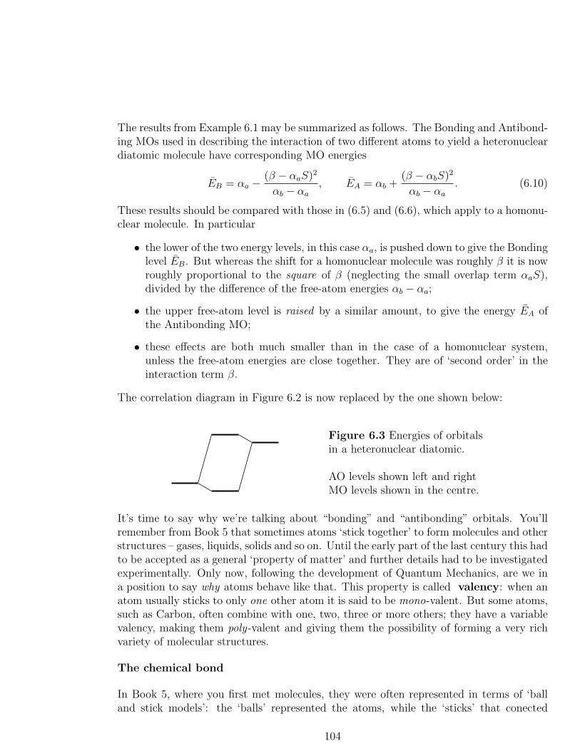
The results from Example 6.1 may be summarized as follows. The Bonding and Antibond-ing MOs used in describing the interaction of two different atoms to yield a heteronucleardiatomic molecule have corresponding MO energies

EB = αa −(β − αaS)

2

αb − αa

, EA = αb +(β − αbS)

2

αb − αa

. (6.10)

These results should be compared with those in (6.5) and (6.6), which apply to a homonu-clear molecule. In particular

• the lower of the two energy levels, in this case αa, is pushed down to give the Bondinglevel EB. But whereas the shift for a homonuclear molecule was roughly β it is nowroughly proportional to the square of β (neglecting the small overlap term αaS),divided by the difference of the free-atom energies αb − αa;

• the upper free-atom level is raised by a similar amount, to give the energy EA ofthe Antibonding MO;

• these effects are both much smaller than in the case of a homonuclear system,unless the free-atom energies are close together. They are of ‘second order’ in theinteraction term β.

The correlation diagram in Figure 6.2 is now replaced by the one shown below:

Figure 6.3 Energies of orbitalsin a heteronuclear diatomic.

AO levels shown left and rightMO levels shown in the centre.

It’s time to say why we’re talking about “bonding” and “antibonding” orbitals. You’llremember from Book 5 that sometimes atoms ‘stick together’ to form molecules and otherstructures – gases, liquids, solids and so on. Until the early part of the last century this hadto be accepted as a general ‘property of matter’ and further details had to be investigatedexperimentally. Only now, following the development of Quantum Mechanics, are we ina position to say why atoms behave like that. This property is called valency: when anatom usually sticks to only one other atom it is said to be mono-valent. But some atoms,such as Carbon, often combine with one, two, three or more others; they have a variablevalency, making them poly-valent and giving them the possibility of forming a very richvariety of molecular structures.

The chemical bond

In Book 5, where you first met molecules, they were often represented in terms of ‘balland stick models’: the ‘balls’ represented the atoms, while the ‘sticks’ that conected

104

them, stood for the chemical bonds that held them together. This is still a widely usedway of picturing molecules of all kinds, ranging from simple diatomics to the giganticstructures studied in the Life Sciences (see Book 9), where the molecules may containmany thousands of atoms arranged in long chains and carrying the genetic code.

Here, however, we are concerned with the ‘sticks’ that join the different atoms: what arethey and how do they work? At bottom, they must be associated with the electrons andnuclei that carry negative and positive electric charge and with their interaction energy.And we have just seen how it is possible for even the single electron of a Hydrogen atomto enter a state of lower energy by bringing up a second proton, so that the electron isattracted to two positive nuclei instead of one. In that case we are imagining the formationof a molecular ion H+

2 , in which the electron occupies a Bonding MO.

Let’s examine this case in more detail. In equation (6.9) we have an expression for theenergy of an electron in the Bonding MO φB, as a function of the parameters α, β, andS (the ‘Coulomb’, ‘resonance’, and ‘overlap’ integrals). These parameters depend on thegeometry of the system (i.e. the positions of the two nuclei) and are not too difficultto calculate in terms of the internuclear separation R. When this is done, the electronicenergy of the system can be plotted against R and is found to increase steadily, goingtowards the energy of a free hydrogen atom, namely −1

2eH, in the long-range limit R→∞.

This is shown in the curve labelled “Electronic energy” in Figure 6.4 (below); but thishas no minimum – which would indicate a stable diatomic system. So what’s wrong?

E = 0

E = −12eH

Internuclear distance R→

Energy

E→

Nuclear repulsion energy

Electronic

energy

Resultantenergy

Figure 6.4 Energy curves for the Hydrogen molecule ion

Resultant energy E has its minimum at R ≈ 2 a0

105

The fact is simply that we haven’t yet included the energy of repulsion between the twonuclei: this is Enuc ∝ (1/R) and goes from a large positive value, when the nuclei are closetogether, to zero when R→∞.We didn’t even include this term in the Hamiltonian (6.1)as it didn’t depend on the electronic variables. Strictly it should be included (the protonsare part of the system!); but then the expectation value E = 〈φ|H|φ〉, for any normalizedstate with wave function φ(r) would contain an additive constant Enuc, which can be putin at the end of the calculation. When this is done, the total energy of the system becomesthe sum of two terms; the repulsion energy Enuc and EB, the energy of the electron in theBonding MO. The two terms are ‘in competition’, one falling as R increases, the otherrising; and together they give a total energy E(R) which shows a shallow minimum at acertain value R = R0. This means there is a chemical bond between the two atoms, with‘bond length’ R0, say. The variation of all three energy terms, as functions of internucleardistance, is shown in Figure 6.4; and the total energy that results behaves as in the curvelabelled “Resultant energy”.

Of course, this is not for the normal hydrogen molecule but rather the molecule ion

that remains when one electron is taken away. However, the energy of H2 behaves ina very similar way: the electronic energy expression has just the same form as for any2-electron system, as given in (2.8). The big difference is that the 1-electron terms,〈Ψ|h(1)|Ψ〉 and 〈Ψ|h(2)|Ψ〉, and the 2-electon term 〈Ψ|g(1, 2)|Ψ〉, are much more difficultto evaluate. Remember that the wave function we’re going to use is a product Ψ(r1, r2) =φB(r1)φB(r2), where both electrons are shown in the Bonding M0 φB, which decribes thestate of lowest energy 2EB when the interelectronic repulsion energy, J = 〈Ψ|g(1, 2)|Ψ〉,is neglected. Since J is positive the total electronic energy will now have a lowest possibleexpectation value

E = 2EB + J,

corresponding to the molecular ground state. This has the same form as that for the2-electron atom; but the 1-electron part, 2EB, will now depend on the attraction of theelectron to both nuclei – and therefore on their separation R, which determines theirpositions in space. Apart from this weak dependence on R, the total electronic energy ofthe system will behave in much the same way as for the ion H+

2 , while the internuclearrepulsion energy remains unchanged as Enuc.

The relevant energy curves for both the normal molecule and its positive ion are thereforerather similar in form. Those for the ion are shown above. The value of R at which theenergy has its minimum is usually called the equilibrium bond length and is denotedby Re while the energy difference between that at the minimum and that for R → ∞is called the dissociation energy, denoted by De. The term “equilibrium” is of coursenot quite correct – the nuclei are in fact moving and it is an approximation to do thecalculation as if they were at rest, for a series of fixed values of R. But it is usually a decentfirst approximation which can later be refined to take account of vibration and rotationof the system around its equilibrium configuration; and anyway we’ve made more seriousapproximations already in using such a simple form of the electronic wave function.

106

6.3 Interpretation of the chemical bond

Figure 6.4 showed the existence of a minimum energy when the two nuclei of a diatomicmolecule were at a certain distance Re, which we called the equilibrium bond length, butoffers no explanation of how the bond originates – where does it come from? But anotherway of saying that the system is in equilibrium is to say that the distribution of electronsmust produce forces, acting on the nuclei, that balance the force of repulsion betweentheir positive charges. And we know already that the electron density function P (r),defined in Chapter 5 for a general many-electron system, will give us a way of calculatingthe energy of interaction between the nuclei and the electron distribution.

The charges on the two nuclei produce an electric field and the potential energy functionfor unit charge at point r in that field will be V (r); so the electron/nuclear interactionenergy for one electron will be −eV (r). When the electronic charge is, in effect, ‘smearedout’ with a density P (r) electrons/unit volume, the total interaction energy will be

Ven =

∫

−eV (r)dr. (6.11)

We now want to know how the contributions to Ven can arise from different parts of theelectron distribution. We start with a very simple example: one electron in an MO, whichmay be of ‘bonding’ or ‘anti-bonding’ type.

Example 6.2 Analysis of the electron density.

Let’s think of an electron in a molecular orbital built up from two atomic orbitals, χ1, χ2, as the linearcombination φ = c1χ1 + c2χ2. The electron density function will then be (using for simplicity normalizedand real MO functions)

P (r) = c 21χ1(r)2 + 2c1c2χ1(r)χ2(r) + c 22χ2(r)

2.

There are three parts to the density, two ‘orbital densities’ and one ‘overlap density’;

d1(r) = χ1(r)2, d2(r) = χ2(r)

2, d12(r) = χ1(bfr)χ2(r)/S12,

where S12 = 〈χ1|χ2〉 and all three terms are therefore normalized to unity. On writing c 21 = P11, c22 =

P22, c1c2 = P12, the electron density takes the form

P (r) = q1d1(r) + q2d2(r) + q12d12(r).

Here q1 = P11, q2 = P22, q12 = 2S12P12 are the quantities of charge, in electron units, associated with the‘orbital’ and ‘overlap’ densities. Provided the MO is correctly normalized, the sum of the qs must be 1electron: q1 + q2 + q12 = 1. The individual qs indicate in a formal way the electron ‘populations’ of thevarious regions in space.

The following Figure 6.5 gives a very schematic picture of the electron distribution in theH+

2 ion, according to the LCAO approximation, for the two states in which the electronoccupies the Bonding MO (left) or the Anti-bonding MO (right).

107

Figure 6.5 Electron density pictures (schematic) see text

The positive nuclei are shown as red dots while the distribution of electronic charge(negative) is shown in lightblue. In the bonding state the nuclei are attracted towardsthe accumulation of negative charge in the bond region (marked by the broken line), theforces acting on them being indicated by the short black arrows. The ‘overlap density’in Example 6.5 contains a quantity of negative charge q12 and this provides most of theattractive force (the separate AO densities being centrosymmetric and giving no net forceon their nuclei). But in the anti-bonding state the overlap density appears with a negativesign and is therefore ‘scooped out’ of the total electron density, the density removed beingindicated in white i.e. as a ‘hole’ in the total density. Note that normalization of the Anti-bonding MO requires that the charge removed from the bond region must go into the twocentrosymmetric AO regions. Each nucleus is therefore pulled towards the enlarged outerparts of the total density, as well as feeling the full Coulomb repulsion of the other nucleus.In this way the origin of the various energy curves in Figure 6.4 receives a nice physicalexplanation.

It is a simple matter to generalize the conclusions from Example 6.5 to a basis containingany number of AOs χi(r) and to any kind of many-electron wave function. We definenormalized AO and overlap densities

di(r) = χi(r)2, dij(r) = χi(r)χj(r)/Sij (6.12)

and write the electron density function in the usual form (cf.(5.29)), taking for simplicityreal functions, P (r) =

∑

ij Pijχi(r)χj(r). In terms of the densities defined in (6.12) itfollows that

P (r) =∑

i

qidi(r) +∑

i<j

qijdij(r), (6.13)

where the orbital and overlap charges are

qi = Pii, qij = 2SijPij (6.14)

and the restriction of the double summation to terms with i < j makes sure that eachoverlap is counted only once.

This conclusion is valid for any N -electron wave function expressed in finite basis formwith any number of basis functions χi, which need not even be AOs (though we oftencontinue to use the term in, for example, the “LCAO approximation”). Nowadays the

108

‘charges’ ‘qi’ and ‘qij ’ are usually called orbital and overlap “populations” of the regionsdefined by the functions χi and their products χiχj; and this way of describing the resultsof electronic structure calculations is called “electron population analysis”. It will be usedoften when we study particular molecules.

6.4 The total electronic energy in terms of density

functions. The force concept in Chemistry

In Chapter 5 we obtained a general expression for the electron density function ρ(x1) foran N -electron system of particles with spin, using xi to denote the space-spin variablesof Particle i. The probability of finding Particle ‘1’ in volume element dx1 = dr1ds1 was

dx1

∫

Ψ(x1,x2, ...xN )Ψ∗(x1,x2, ...xN)dx2 ... dxN ,

obtained by integrating over all ‘positions’ of the other particles. And, since the sameresult will be obtained for whichever electron is found in volume element dx1 at pointx1, multiplication by N will give equation (5.24). Thus, the probability/unit volume offinding a particle, no matter which, at point x1 will be

ρ(x1) = N

∫

Ψ(x1,x2, ...xN )Ψ∗(x1,x2, ...xN)dx2 ... dxN . (6.15)

Remember that this is the probability density with spin variable included. If we’re notinterested in spin it’s enough to sum over both spin possibilities by integrating over thespin variable s1 to obtain a spinless density function P (r1) =

∫

ρ(x1)ds1. The resultis the probability density for finding a particle, of either spin in a volume element r1(e.g. dx1dy1dz1) at point r1 in ordinary 3-space. If you look back at Examples 5.6 and5.7 in the last chapter you’ll find that you’ve done all this before for atoms, thinkingmainly of IPM-type wave functions. But the results apply to any kind of wave function(approximate or exact and for any kind of system). So now we’re ready to deal withmolecules.

The 1- and 2-electron density matrices, including dependence on spin variables, are

ρ(x1;x′1) and π(x1,x2;x

′1,x

′2).

They determine the expectation values of operator sums, such as∑

i h(i) and∑

i,j g(i, j),in any state Ψ. For example

〈Ψ|∑i h(i)|Ψ〉 =∫

x′

1→x1

h(1)ρ(x1;x′1)dx.

From now on, to simplify the text, let’s remember that the primes are only needed whenan operator works on a density matrix, being removed immediately after the operation –so we’ll stop showing them, writing the expectation values as

109

〈Ψ|∑i h(i)|Ψ〉 =∫

h(1)ρ(x1)dx1,

〈Ψ|∑i,j g(i, j)|Ψ〉 =∫

g(1, 2)π(x1,x2)dx1dx2.

(6.16)

and remembering what the short forms mean.

When tiny spin-dependent terms are neglected these results may be reduced in terms ofthe ‘spinless’ density matrices P (r1; r

′1) and Π(r1, r2; r

′1, r

′2). The counterparts of (6.16)

apply when the operators do not touch the spin variables; they become instead

〈Ψ|∑i h(i)|Ψ〉 =∫

h(1)P (r1)dr1,

〈Ψ|∑i,j g(i, j)|Ψ〉 =∫

g(1, 2)Π(r1r2)dr1dr2

(6.17)

and involve only the position variables of typical particles

In what follows we’ll use the reduced forms in (6.17), which apply when relativistic correc-tions are ignored. The total electronic energy of any system of N electrons, moving arounda set of fixed nuclei, can then be expressed in a very simple and transparent form. The 1-electron operator for an electron at point r1 in ordinary 3-space is h(1) = −1

2∇2(1)+V (r1)

(kinetic energy plus potential energy in field of the nuclei), while the 2-electron operatorfor electrons at points r1 and r2 is simply the Coulomb repulsion energy, g(1, 2) = 1/r12 (inatomic units), r12 being the interelectronic distance (the length of the vector separationr2 − r1). On putting these terms in the energy expectation value formula E = 〈Ψ|H|Ψ〉,we find (do it!)

E= -12

∫

∇2(1)P (r1)dr1 +

∫

V (1)P (r1) +12

∫

g(1, 2)Π(r1, r2)dr1dr2

(6.18)

Here the three terms are, respectively, T the total kinetic energy; Ven, the potential energyof a smeared out electronic charge in the field of the nuclei; and the average potentialenergy Vee due to pairwise repulsions described by the 2-electron density Π(r1, r2).

110

The Hellmann-Feynman theorem

In Section 6.3 we gave a pictorial interpretation of the chemical bond in terms of theelectron density function P (r). According to classical physics, the positively chargednuclei in a molecule would ‘feel’ the forces due to the distribution of negative charge inwhich they were embedded. But in quantum mechanics the function P (r) gives only theprobability of finding an electron at point r in 3-space; we must show that the systembehaves as if this function were a density of negative charge. We must define the forceacting on any nucleus in terms of things like the energy – which we know how to calculate.

To do that we first imagine the molecule to be in equilibrium, the total energy beingstationary against small changes of any kind – in the wave function and in the potentialenergy function V (r) (e.g. due to a field applied from outside the molecule, or change ofnuclear positions). Since

E =

∫

h(1)P (r1)dr1 +12

∫

g(1, 2)Π(r1, r2)dr1dr2,

the first-order changes to be considered result from δh and the density functions δP (1) andδΠ(1, 2). The total first-order energy change will therefore be (noting that the operators∇2(1) and g(1, 2) remain unchanged)

δE =

∫

δh(1)P (r1)dr1 +

∫

h(1)δP (r1)dr1 +12

∫

g(1, 2)δΠ(r1, r2)dr1dr2 (6.19)

and the stationary value condition will follow on equating this quantity to zero.

Now suppose that the density functions have been fully optimized by varying the energyin the absence of any perturbation term δh(1). In that case only the last two terms remainin (6.19) and their sum must be equated to zero. Thus

The first-order energy change arising fromthe perturbation h(1)→ h(1) + δh(1)

is given by δE =

∫

δh(1)P (r1)dr1,

provided the wave function Ψ is fully optimizedin the absence of the perturbation.

(6.20)

This is usually called the “Hellmann-Feynman theorem in its general form”. It wasdiscovered by Hellmann (1937) for the special case where the perturbation was due to achange of nuclear position and independently, two years later, by Feynman. In thinkingabout the forces that hold the nuclei together in a molecule we first have to define them: ifwe move one nucleus, nucleus n say, through a distance δXn in the direction of the x-axis,we’ll change the total energy of the molecule by an amount δE given in (6.20). And in

111

this case δh(1) = δVn(r1), the corresponding change in potential energy of an electron atpoint r1 in the field of the nucleus.

Now the rate of decrease of this potential energy is the limiting value of −δVn(r1)/δXn

as Xn → 0 and measures the x-component of the force acting between Nucleus n and anelectron at point r1. Thus we may write

−∂Vn(r1)∂Xn

= Fnx(r1)

and this defines the force component on Nucleus n due to an electron at r1.

A similar argument applies to the total electronic energy E due to interaction with allthe electrons: its rate of decrease on moving Nucleus n through a distance Xn will be−∂E/∂Xn and will give the x-component Fnx of the total force exerted on Nucleus n byall the electrons. Thus

− ∂E

∂Xn

= Fnx

defines the x-component of total force on Nucleus n due to interaction with the wholeelectron distribution.

Having defined the forces, in terms of energy derivatives, we return to (6.20). Here,putting δh(1) = δVn(r1), dividing by δXn and going to the limit δXn → 0, we find

Fnx =

∫

Fnx(r1)P (r1)dr1. (6.21)

In words, the x-component of the total force on any nucleus (n) may be computed byadding (integrating) the contributions arising from all elements of the charge cloud. Thisis true for any component and therefore the force vector acting on any nucleus in themolecule can be calculated in exactly the same way: once the electron density has beencomputed by quantum mechanics the forces holding the nuclei together may be givenan entirely classical interpretation. When the molecule is in equilibrium it is becausethe forces exerted on the nuclei by the electron distribution are exactly balanced by therepulsions between the nuclei – as they were in Figure 6.4.

This beautiful result seems too good to be true! Apparently only the electron densityfunction P (r1) is needed and the 2-electron function Π(r1, r2), which is vastly more difficultto calculate, doesn’t come into the picture. So what have we overlooked?

In deriving (6.21) we simply took for granted that the variational wave function Ψ wasfully optimized, against all the parameters it may contain. But in practice that is hardlyever possible. Think, for example, of an LCAO approximation, in which the atomicorbitals contain size parameters (orbital exponents) and the coordinates of the pointsaround which they are centred: in principle such parameters should be varied in theoptimization, allowing the orbitals to expand or contract or to ‘float away’ from thenuclei on which they are located. In practice, however, that is seldom feasible and theHellmann-Feynman theorem remains an idealization – though one which is immenselyuseful as a qualitative tool for understanding molecular structure even at a simple level.

112

Chapter 7

Molecules: Basic Molecular Orbital

Theory

7.1 Some simple diatomic molecules

We start this chapter by going back to the simple theory used in Chapter 6, to see howwell it works in accounting for the main features of molecules formed from the elementsin the first row of the Periodic Table.

In Section 6.2 we studied the simplest possible diatomic system, the Hydrogen moleculepositive ion H+

2 , formed when a proton approaches a neutral Hydrogen atom. And evenin Chapter 5 we had a glimpse of the Periodic Table of all the elements: the first tenatoms, with their electron configurations, are

Hydrogen[1s1] Helium[1s2] Lithium[1s22s1] Beryllium[1s22s2]

in which the first two s-type AOs are filling (each with up to two electronsof opposite spin component, ±1

2), followed by six more, in which the p-type

AOs (px, py, pz) are filling with up to two electrons in each.

Boron[1s22s22p1] Carbon[1s22s22p2] Nitrogen[1s22s22p3]

Oxygen[1s22s22p4] Fluorine[1s22s22p5] Neon[1s22s22p6]

Helium, with two electrons in the 1s shell, doesn’t easily react with anything; it is thefirst Inert Gas atom. So let’s turn to Lithium, with one 2s electron outside its (1s)2 innershell, and ask if this would react with an approaching atom of Hydrogen. We could, forexample, try to calculate the total electronic energy E using the Self-Consistent Fieldmethod (see Chapter 4) and then adding the nuclear repulsion energy, as we did for themolecule H2 in Section 6.2. Again, as we don’t have any ‘ready-made’ molecular orbitals

113

we have to build them out of a set of basis functions, χ1, χ2, ... χi ... and it seems mostreasonable to choose these as the atomic obitals of the atoms we are dealing with, writingthe MO φ as

φ = c1χ1 + c2χ2 + ... ... cmχm (7.1)

for a basis of m functions. This is the famous LCAO (linear combination of atomicorbitals) approximation, which is the one most widely used in molecular structure cal-culations. In principle, if the basis set is large enough, this could be a fairly accurateapproximation.

As you learnt in Chapter 4 (you should go back there for the details) the MOs shouldreally be determined by solving the operator equation

Fφ = ǫφ [the Hartree− Fock equation] (7.2)

but the best we can do, in LCAO approximation, is to choose the expansion coefficientsso as to minimize the calculated value of the total electronic energy E. The best approx-imate MOs of the form (7.1), along with their corresponding orbital energies (ǫ) are thendetermined by solving the secular equations

Fc = ǫc, (7.3)

where c is the column of expansion coefficients in (7.1) and F is the square matrix repre-senting the effective Hamiltonian F – which has elements Fij = 〈χi|F|χj〉.(Note that this simple form of the secular equations, depends on using orthogonal basis functions; butif overlap is not small enough to be neglected it may be removed by choosing new combinations – workwhich is easily done by modern computers.)

In a first example, we summarize an early SCF calculation on the LiH system.

Example 7.1 The Lithium Hydride molecule: LiH.

In the SCF calculation by Ransil (1960) the AO basis used consisted of the 1s, 2s and 2p orbitals ofthe Lithium atom, together with a single 1s orbital for the Hydrogen. The basis functions were thusχ1s, χ2s, χ2p, χH , where the first three are centred around the Li nucleus (only one p function is needed,that with symmetry around the bond axis) and the last is a 1s-type function, centred on the proton. TheLithium 1s AO is tightly localized around the nucleus (Z = 3) and in good approximation does not mixwith the other functions. The MOs that come from the 4-electron SCF calculation are then found to be

φ1σ ≈ χ1s; φ2σ ≈ 0.323χ2s + 0.231χ2p + 0.685χH .

The electron configuration of the molecule will then be, with four electrons, LiH[1σ22σ2].

This indicates a Lithium inner shell, similar to that in the free atom, and a bonding MO 2σ containing2 electrons. But the bonding MO is not formed from one 2s AO on the Lithium atom, overlapping withthe Hydrogen 1s AO; instead, it contains two AOs on the Lithium atom. If we want to keep the simplepicture of the bond, as resulting from the overlap of two AOs, one on each atom, we must accept thatthe ‘AO’s need not be ‘pure’ but may be mixtures of AOs on a single centre. Ransil’s calculation showsthat a much clearer description of LiH is obtained by rewriting his MO in the form

φ2σ ≈ 0.397χhyb + 0.685χH ,

114

where χhyb = 0.813χ2s+0.582χ2p is called a hybrid orbital and this kind of mixing is called hybridization.

The general form of this Lithium hybrid AO is indicated below in Figure 7.1, in which the contour lines

correspond to given values of the function χhyb. The broken line marks the ‘nodal surface’ separating

negative and positive values of χhyb. The energy is lowered by hybridization, which increases the strength

of the bonding by putting more electron density (i.e. negative charge) between the positive nuclei; but

this is offset by the energy ǫ2p − ǫ2s needed to ‘promote’ an electron from a 2s state to a 2p state. So

hybridization is favoured for AOs of similar energy and resisted when their energy difference is large.

Figure 7.1 Contour map for the s-p hybrid orbital χhyb

The capacity of an atom to form chemical bonds with other atoms is known as valencyand is often measured by the number of bonds it can form. Lithium in LiH is mono-

valent, but Oxygen in H2O is di-valent and Carbon in CH4 is quadri-valent. But manyatoms show variable valency, depending on the nature of the atoms they combine withand on the degree of hybridization involved. In Example 7.1 the Lithium atom is said tobe in a “valence state”, depending on the degree of 2s-2p mixing, and this may usefullybe decribed in terms of the electron populations introduced in Section 6.3. If the hybridorbital is written as the mixture χhyb = aχ2s+bχ2p, an electron in χhyb gives a probabilitydensity Phyb = a2χ 2

2s+b2χ 2

2p+2abχ2sχ2p. Integration over all space gives unity (1 electron),with a2 coming from the 2s density, b2 from the 2p and nothing from the last term (theAOs being orthogonal). We can then say that the 2s and 2p AOs have electron populationsa2 and b2, respectively, in the molecule. The electron configuration of the Lithium atom,in the molecule, could thus be written Li[1s22s0.6612p0.339] (according to Example 7.1)the numbers being the values of a2 and b2 for an electron in the ‘valence orbital’ χhyb.The atom never actually passes through a ‘valence state’; but the concept is none theless valuable. For example, the idea that a fraction of an electron has been ‘promoted’from a 2s orbital to an empty 2p shows why hybridization, to produce strong bonds, ismost common for elements on the left side of the Periodic Table, where the 2s-2p energyseparation is small.

Now let’s try something a bit more complicated. If we replace Lithium by Carbon weshall have four electrons outside the tightly-bound 1s shell, two of them in the next-higherenergy 2s orbital and two more in the slightly-higher energy 2p orbitals (2px,2py,2pz).These four are not too strongly bound to prevent them taking part in bonding with otheratoms, so they are are all available as valence electrons. And if we go two places further

115

along the First Row we come to Oxygen, which has six electrons outside its 1s2 inner shell– all available, to some degree, for bonding to other atoms. The energy difference betweenthe 2s and 2p orbitals increases, however, with increasing nuclear charge; and as a resultthe elements C and O have rather different valence properties. In the next example we’lltry to understand what can happen when these two atoms come together and begin toshare their valence electrons.

Example 7.2 The Carbon monoxide molecule: CO.

The 1s2 inner shells, or ‘cores’, of both atoms are so strongly bound to their nuclei that the main effectthey have is to ‘screen’ the positive charges (Ze, with Z=6 for the carbon atom and Z=8 for oxygen); the‘effective’ nuclear charges are then closer to Zeff = 4, for C, and 6 for O. We’ll therefore think aboutonly the valence electrons, asking first what MOs can be formed to hold them.

We already know that the AOs on two different atoms tend to combine in pairs, giving one bondingMO along with an anti-bonding partner; and that this effect is more marked the more strongly the AOsoverlap. Think of the 2s AOs as spheres and the 2p AOs as ‘dumbells’,

+−

Here the + and − parts indicate regions in which the wave function χ is positive or negative. Unlikean s-type AO, one of p-type is associated with a definite direction in space, indicated by the arrow. Forthe CO molecule, the 2s AOs on the two centres will not overlap strongly as they come together, owingto their size difference (the oxygen 2s being smaller – can you say why?). They might give a weaklybonding MO, consisting mainly of the oxygen 2s AO, which we’ll call 1σ∗

s ) as it would be the first MOwith rotational symmetry around the 2-centre axis. On the other hand, the oxygen 2pz AO pointingalong the axis towards the carbon would have a fairly good overlap with the carbon 2s AO. In that casewe might expect, as usual, two MOs; one bonding (call it 2σs) and the other anti-bonding (2σ∗

s .)

However, there are three 2p AOs on each centre, the 2px and 2py, both transverse to the bond axis (alongwhich we’ve directed the 2pz AO). They are of π-type symmetry and, when pairs of the same type comeclose together, they will have a good side-to-side or ‘lateral’ overlap:

+

−

+

−

In summary, the orbitals available for holding the 10 valence electrons would seem to be

•1σ – the first MO of σ type, mainly Oxygen 2s

•2σ – a bonding MO, formed from Carbon 2s and Oxygen 2pz

•3σ – an anti-bonding MO, the partner of 2σ

•1πx – a π-bonding MO, formed from 2px AOs on C and O

•1πy – a π-bonding MO, formed from 2py AOs on C and O

To assign the electrons to these MOs we look at the probable correlation diagram.

116

The correlation diagram for the CO molecule, with neglect of hybridization on one orboth atoms, would seem to be that shown below in Figure 7.2:

2p

2s

Carbon

2π

4σ3σ

1π

2σ

1σ

CO

2p

2sOxygen

Figure 7.2 Correlation diagram for CO, no hybrids

Notice that the 2p AOs take part in both σ− and π-type MOs: the 2σ and 3σ MOs willeach have a 2pz component (also symmetrical around the CO axis) while the 1π MO isdegenerate, with 1πx and 1πy MOs containing only 2px and 2py AOs, respectively. The1πx and 1πy MOs are formed from the ‘side-by-side’ overlap of 2p AOs perpendicular tothe CO axis (shown pictorially in Example 7.2). The highest occupied MO (often calledthe ”HOMO”) is 3σ and is apparently anti -bonding.

This all looks a bit strange, because we know from Example 1 that the mixing of AOs islikely to be much more widespread, mixtures of AOs on each centre giving 1-centre hybridswhich can better describe the results of a good SCF calculation. Moreover, experimentshows the picture to be quite wrong! In particular the main CO σ bond is very strong,while here it would be largely ‘cancelled’ by the anti-bonding effect of the electrons inthe 3σ MO. There is also evidence for a lone pair of electrons smeared out behind theCarbon, but here there seems to be no MO to hold them. We must ask how this pictureis changed on admitting hybridization: the conclusion is shown in Figure 7.3 below.

2p

2s

Carbon

h2

h1

4σ

3σ

2σ

1σ

CO

2p

2sOxygen

h2

h1

Figure 7.3 Correlation diagram for CO, with hybrid AOs

Even without doing a full SCF calculation, a qualitative argument leads easily to the sameconclusion. By allowing for the mixing of 2s and 2p AOs on Carbon and on Oxygen (s and

117

p orbital energies being fairly close together), the correlation diagram in Figure 7.2 mustbe re-drawn. The result is that shown in Figure 7.3, where the 2s and 2p orbital energiesare again indicated on the extreme left (for Carbon) and extreme right (for Oxygen). Butnow, when these AOs are allowed to mix – forming hybrids, the (2s) AO of lower energymust be raised in energy – owing to the inclusion of a bit of 2p character; while the energyof an electron in the upper AO must be lowered, by inclusion of 2s character. The effectsof s-p hybridization are indicated by the broken lines connecting the hybrid energies withthe energies of their ‘parent’ AOs.

The probable orbital energies of the MOs in the CO molecule are shown in the centre ofthe diagram. The broken lines now show how the MO energy levels arise from the hybridlevels to which they are connected. The energies of the π-type MOs are not affected bythe hybridization (containing only 2px and 2py AOs) and remain as in Figure 7.2 – withthe 1π level (not shown)lying between the 2σ and 3σ MO energies.

When we assign the 10 valence electrons to these MOs we find

• a pair of electrons in the 1σ MO, which is mainly Oxygen 2s;

• a pair in the 2σ MO, the bonding combination of strongly overlapping hybrids, pointingtowards each other along the bond axis;

• two pairs in the bonding 1π-type MOs, transverse to the bond axis; and

• a pair in the 3σ MO, which is mainly a Carbon hybrid and is too high in energy to mixwith σ-type AOs on the other atom.

Now let’s look at the electron density (density of negative charge), which is given, as afunction of position in space, by |φ|2 for an electron in the MO φ. (If you’re not yet readyto follow all the details you can skip the following part, in small type, and come back toit later.)

The first MO (above) gives a density |φ|2 roughly spherical and strongly bound to the Oxygen 1s2 ‘core’,but leaning slightly away from the Carbon (can you say why?)

The second MO gives a density concentrated on and around the CO axis, between the two atoms,providing a strong σ bond

The third MO is degenerate, with density contributions |φx|2 and |φy|2 where, for example, φx = caφa2px

+

cbφb2px

– a linear combination of 2px AOs on the two atomic centres. At a general point P(x, y, z), a2px AO has the form xf(r), where distances are measured from the nucleus and the function f(r) isspherically symmetrical. If you rotate a 2px AO around the z axis it will change only through the factorx; and the same will be true of the combination φx.

The whole electron density function will thus change only through a factor x2 + y2 = r 2z , where rz is the

distance of Point P from the CO bond axis. A ‘slice’ of density, of thickness dz, will be a circular disk ofcharge – with a hole in the middle because rz falls to zero on the bond axis. The two π bonds togethertherefore form a hollow ‘sleeve’ of electron density, with the σ distribution inside – along the axis.

The 3σ HOMO now comes below the 4σ anti-bonding MO and does not diminish the strong σ bond inany way. It provides essentially a lone-pair electron density, localized mainly on the Carbon. Moreover,this density will point away from the CO σ-bond because h2 and h1 stand for orthogonal orbitals – andh1 points into the bond.

In summary, it seems that when hybridization is admitted everything can be understood!

118

The CO molecule should have a triple bond, a strong σ bond supported by two weakerπ bonds; and the Carbon should have a region of lone-pair electron density on the sideaway from the C≡O triple bond – all in complete agreement with its observed chemicalproperties.

7.2 Other First Row homonuclear diatomics

The CO molecule has 10 (=4+6) valence electrons outside the 1s2 cores and is therefore‘isoelectronic’ with the Nitrogen molecule, N2, which is homonuclear and therefore hasa symmetrical correlation diagram. The molecules, Nitrogen (N2,) Oxygen (O2) andFluorine (F2), with 10, 12 and 14 valence electrons, respectively, all have similar energy-level diagrams; but differ in the way the levels are filled as electrons are added. This is allpart of the so-called “aufbau approach” (“aufbau” being the German word for “buildingup”) in which electrons are added one at a time to the available orbitals, in ascendingorder of orbital energy. The First Row atoms use only 1s,2s and 2p AOs, in which onlythe 2s and 2p AOs take part in molecule building (see for example Figure 7.2). But inhomonuclear diatomics the two atoms are identical and the correlation diagram is simplerbecause orbitals of identical energy interact very strongly and hybridization may often beneglected. For First Row atoms a typical diagram is shown in Figure 7.4, below.

2p

2s

Nitrogen

1π∗

1π

2σ∗

2σ

1σ∗

1σ

N2

2p

2s

Nitrogen

Figure 7.4 Correlation diagram for N2, no hybrids

Note that the 2s AOs give rise to the bonding and anti-bonding MOs denoted by 1σ and2σ (first and second valence MOs of σ symmetry, but the 2p AOs, three on each centre,give MOs of both σ and π type. For clarity it is sometimes useful to use an alternativenotation in which, for example, the first valence MO and its anti-bonding partner arecalled 1σ and 1σ∗. The MOs can then be put in order of increasing energy and displayedas

1σ ⇒ 1σ∗ ⇒ 2σz ⇒ (1πx, 1πy) ⇒ (1π∗x, 1π

∗y) ⇒ 2σ∗

z

119

where the arrows indicate increasing order of orbital energies and the subscript z refers tothe bond axis, while x and y label the transverse axes. The π-type MOs are degenerate,x and y components having identical energies.

The electron configurations of most of the homonuclear diatomics in the First Row con-form to the above order of their MO energy levels. Let’s take them one at a time, startingagain with Nitrogen.

Nitrogen

Following the aufbau procedure, the first two of the ten valence electrons should go intothe 1σ MO with opposite spins; the next two will go into its antibonding partner 1σ∗ –more or less undoing the bonding effect of the first pair; two more go into the 2σz MOwhich is strongly bonding, being formed from 2pz AOs pointing towards each other. Butthen there are four MOs, all of π type, formed from the 2px and 2py AOs on the twoatoms, which are perpendicular to the σ bond: they are 1πx, 1πy and their anti-bondingpartners (1π∗

x, 1π∗y) – all before we come to 2σ∗

z , which is well separated from 2σz owingto the strong overlap of the component 2pz AOs. The remaining four of the 10 valenceelectrons nicely fill the two bonding MOs and give two bonds of π type.

The end result will be that N2 has a triple bond and the electron configuration

1σ2 1σ∗ 22σ2z 1π

2x 1π

2y .

The next First Row diatomic will be

Oxygen

Here there are 12 valence electrons, two more than in N2, and they must start fillingthe anti -bonding π-type MOs. But we know that when two orbitals are degenerateelectrons tend to occupy them singly: so 1π∗

x1 1π∗

y1 is more likely than, say, 1π∗

x2. And

each antibonding π electron will ‘cancel’ half the effect of a bond pair.

The probable result is that O2 will have a double bond and an electron configuration suchas

1σ2 1σ∗2 2σ2z 1π

2x 1π

2y 1π

∗x1 1π∗

y1.

Moreover, the electrons in the singly-occupied MOs may have their spins parallel-coupled– giving a triplet ground state (S = 1). This means that Oxygen may be a paramagnetic

molecule, attracted towards a magnetic field. All this is in accord with experiments in thelaboratory. Of course, the ‘theory’ we are using here is much too simple to predict thingslike spin coupling effects (we haven’t even included electron interaction!) but experimentconfirms that the last two electrons do indeed have their spins parallel-coupled to give atriplet state.

Fluorine

The electron configuration for the molecule F2 is obtained by adding two more valenceelectrons. This will complete the filling of the π-type anti-bonding MOs, to give theconfiguration

1σ2 1σ∗2 2σ2z 1π

2x 1π

2y1π

∗x21π∗

y2.

120

The pairs of electrons in the 1π∗x and 1π∗

y MOs then take away the effect of those in thecorresponding bonding MOs, removing altogether the π bonding to leave a single σ bond.Neon

The molecule Ne2 does not exist! Neon is an inert gas, like Helium, its atoms not formingcovalent bonds with anything. The reason is simply that, on adding two more electrons,every bonding MO has an anti-bonding partner that is also doubly occupied. Every Rowof the Periodic Table that ends with the filling of a ‘shell’ of s- and p-type AOs has alast atom of inert-gas type: the inert-gas atoms are Helium (He), Neon (Ne), Argon (A),Krypton (Kr), Xenon (Xe), Radon (Rn), with values of the principal quantum number ngoing from n = 1 up to n = 6.

Here we are dealing only with the First Row, that ends with Neon and contains only thefirst 10 elements, but we started from Nitrogen (atomic number Z = 7) and continued inorder of increasing Z. The atom before that is Carbon, the most important of the oneswe left out. So let’s do it now.

Carbon

Carbon has only 4 valence electrons outside its 1s2 core, so if a C2 molecule exists weshould have to assign 8 electrons to energy levels like the ones shown in Figure 7.4 –corresponding to the MOs

1σ, 1σ∗, 2σz, (1πx, 1πy), (1π∗x, 1π

∗y), 2σ∗

z .

Before we start, however, remember that the s- and p-type energy levels get closer togetheras the effective nuclear charge (Zeff ≈ Z− 2) gets smaller; and this means that the 2s and2pz AOs must be allowed to mix, or ‘hybridize’, as in Figure 7.3, where the mixing givesrise to hybrids h1 and h2. h1 is largely 2s, but with some 2pz which makes it ‘lean’ intothe σ bond; h2, being orthogonal to h1, will be largely 2pz, but pointing away from thebond. This will be so for both Carbons. The correlation diagram should then have theform

h2

h1

Carbon

1π∗

1π

2σ∗

2σ1σ∗

1σ

C2

h2

h1

Carbon

Figure 7.5 Correlation diagram for C2, with hybrids

– where the h1 and h2 levels are now relatively close together and the order of the MOlevels they lead to is no longer ‘standard’. The order in which they are filled up, in the

121

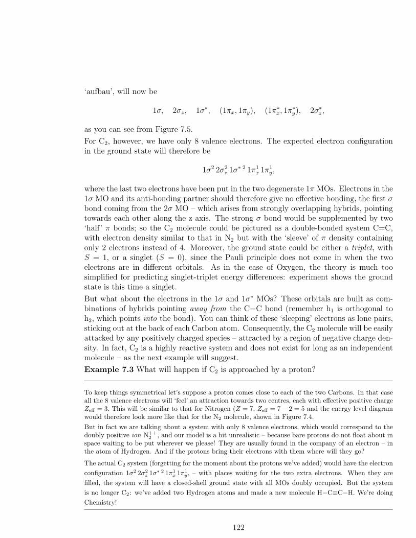
‘aufbau’, will now be

1σ, 2σz, 1σ∗, (1πx, 1πy), (1π∗x, 1π

∗y), 2σ∗

z ,

as you can see from Figure 7.5.

For C2, however, we have only 8 valence electrons. The expected electron configurationin the ground state will therefore be

1σ2 2σ2z 1σ

∗ 2 1π1x 1π

1y ,

where the last two electrons have been put in the two degenerate 1π MOs. Electrons in the1σ MO and its anti-bonding partner should therefore give no effective bonding, the first σbond coming from the 2σ MO – which arises from strongly overlapping hybrids, pointingtowards each other along the z axis. The strong σ bond would be supplemented by two‘half’ π bonds; so the C2 molecule could be pictured as a double-bonded system C=C,with electron density similar to that in N2 but with the ‘sleeve’ of π density containingonly 2 electrons instead of 4. Moreover, the ground state could be either a triplet, withS = 1, or a singlet (S = 0), since the Pauli principle does not come in when the twoelectrons are in different orbitals. As in the case of Oxygen, the theory is much toosimplified for predicting singlet-triplet energy differences: experiment shows the groundstate is this time a singlet.

But what about the electrons in the 1σ and 1σ∗ MOs? These orbitals are built as com-binations of hybrids pointing away from the C−C bond (remember h1 is orthogonal toh2, which points into the bond). You can think of these ‘sleeping’ electrons as lone pairs,sticking out at the back of each Carbon atom. Consequently, the C2 molecule will be easilyattacked by any positively charged species – attracted by a region of negative charge den-sity. In fact, C2 is a highly reactive system and does not exist for long as an independentmolecule – as the next example will suggest.

Example 7.3 What will happen if C2 is approached by a proton?

To keep things symmetrical let’s suppose a proton comes close to each of the two Carbons. In that caseall the 8 valence electrons will ‘feel’ an attraction towards two centres, each with effective positive chargeZeff = 3. This will be similar to that for Nitrogen (Z = 7, Zeff = 7− 2 = 5 and the energy level diagramwould therefore look more like that for the N2 molecule, shown in Figure 7.4.

But in fact we are talking about a system with only 8 valence electrons, which would correspond to thedoubly positive ion N++

2 , and our model is a bit unrealistic – because bare protons do not float about inspace waiting to be put wherever we please! They are usually found in the company of an electron – inthe atom of Hydrogen. And if the protons bring their electrons with them where will they go?

The actual C2 system (forgetting for the moment about the protons we’ve added) would have the electron

configuration 1σ2 2σ2z 1σ

∗ 2 1π1x 1π

1y, – with places waiting for the two extra electrons. When they are

filled, the system will have a closed-shell ground state with all MOs doubly occupied. But the system

is no longer C2: we’ve added two Hydrogen atoms and made a new molecule H−C≡C−H. We’re doing

Chemistry!

122

Of course, the orbitals in the new molecule H−C≡C−H, which is called Acetylene, arenot quite the same as in C2: the lone-pair orbitals (h2), which we imagined as “stickingout at the back of each Carbon atom” now have protons embedded in them and describetwo C−H bonds. Here, in dealing with our first polyatomic molecule, we meet a newproblem: acetylene apparently has two CH single bonds and one CC triple bond. Weare thinking about them as if they were independently localized in different regions ofspace; but in MO theory the bonding is described by non-localized orbitals, built up aslinear combinations of much more localized AOs. All the experimental evidence pointstowards the existence of localized bonds with characteristic properties. For example,the bond energies associated with CC and CH links are roughly additive and lead tomolecular heats of formation within a few per cent of those measured experimentally.Thus, for acetylene, taking the bond energies of C−H and C≡C as 411 and 835 kJ mol−1,respectively, gives an estimated heat of formation of 1657 kJ mol−1 – roughly the observedvalue. (If you’ve forgotten your Chemistry you’d better go back to Book 5; Science is allone!)

Next we’ll ask if similar ideas can be applied in dealing with other polyatomic molecules.

7.3 Some simple polyatomic molecules;

localized bonds

The discussion of H−C≡C−H can easily be put in pictorial form as follows. Each Carbonatom can be imagined as if it were in a valence state, with two of its four valenceelectrons in hybrid orbitals sticking out in opposite directions along the z axis and theother two in its 2px and 2py AOs. This state can be depicted as

•z-axis

x

y

where the Carbon is shown as the bold dot in the centre, while the bold arrows stand forthe hybrids h1 and h2, pointing left and right. The empty circles with a dot in the middleindicate they are singly occupied. The arrows labelled ‘x’ and ‘y’ stand for the 2px and2py AOs, pointing in the positive directions (− to +), and the circles each contain a dotto stand for single occupation.

The electronic stucture of the whole molecule H−C≡C−H can now be visualized as

123

•C •C

• •H C C H

where the upper diagram represents the two Carbon atoms in their valence states (π-typeMOs not indicated); while the lower diagram shows, in very schematic form, the electronicstructure of the molecule H−C≡C−H that results when they are brought together andtwo Hydrogens are added at the ends. The C≡C triple bond arises from the σ-type singlebond, together with the πx- and πy-type bonds (not shown) formed from side-by-sideoverlap of the 2px and 2py AOs. The two dots indicate the pair of electrons occupyingeach localized MO.

Acetylene is a linear molecule, with all four atoms lying on the same straight line. Butexactly the same principles apply to two- and three-dimensional systems. The Methyl

radical contains four atoms, lying in a plane, Carbon with three Hydrogens attached.Methane contains five atoms, Carbon with four attached Hydrogens. The geometricalforms of these systems are experimentally well known. The radical (so-called because itis not a stable molecule and usually has a very short lifetime) has its Hydrogens at thecorners of an equilateral triangle, with Carbon at the centre; it has been found recentlyin distant parts of the Universe, by astronomical observation, and suggests that Life mayexist elswhere. Methane, on the other hand, is a stable gas that can be stored in cylindersand is much used in stoves for cooking; its molecules have four Hydrogens at the cornersof a regular tetrahedron, attached to a Carbon at the middle. These shapes are indicatedin Figure 7.6 below.

2

3

1

4

3

1 2

Figure 7.6 Shapes of the Methyl radical and the Methane molecule

In the Figure the large black dots indicate Carbon atoms, while the smaller ones showthe attached Hydrogens. In the Methyl radical (left) the Hydrogens are at the cornersof a flat equilateral triangle. In Methane (right) they are at the corners of a regular

tetrahedron, whose edges are shown by the solid lines. The tetrahedron fits nicelyinside a cube, which conveniently tells you the coordinates of the four Hydrogens: usingex ey, ez to denote unit vectors parallel to the cube edges, with Carbon as the origin, unitsteps along each in turn will take you to H4 (top corner facing you) so its coordinates will

124

be (1,1,1). Similarly, if you reverse the directions of two of the steps (along ex and ey,say) you’ll arrive at H3, the ‘back’ corner on the top face, with coordinates (−1,−1, 1).And if you reverse the steps along ey and ez you’ll get to H1 (left corner of bottom face),while reversing those along e1 and e3 will get you to H2 (right corner of bottom face).

That’s all a bit hard to imagine, but it helps if you make a better drawing, with ez asthe positive z axis coming out at the centre of the top face, ex as the x axis coming outat the centre of the left-hand face, and ey as the y axis coming out at the centre of theright-hand face. Keep in mind the definition of a right-handed system; rotating the x axistowards the y axis would move a corkscrew along the z axis.

In fact, however, it’s easiest to remember the coordinates of the atoms themselves: theywill be H4(+1,+1,+1) – top corner facing you; H3(-1,-1,+1) – top corner behind it;

H2(+1,-1,-1) – bottom corner right; H1(-1,+1,-1) – bottom corner left and that meanstheir position vectors are, respectively,

h4 = ex + ey + ez, h3 = −ex − ey + ez, h2 = ex − ey − ez, h1 = −ex + ey − ez,

relative to Carbon at the origin.

The Methyl radical is easier to deal with, being only 2-dimensional. A bit of simplegeometry shows that (taking the Carbon atom as origin (0,0), with Hydrogens on aunit circle, x axis horizontal and y axis vertical) the Hydrogens have coordinates H1(1, 0),H2(−1

2, 12

√3), H3(−1

2,−1

2

√3). Their position vectors are thus (given that

√3 = 1.73205)

h1 = ex, h2 = −0.5ex + 0.8660ey, h3 = −0.5ex − 0.8660ey.

Example 7.4 An sp hybrid pointing in any direction

How can we get sp hybrids that point from the Carbon atoms in Figure 7.6 to all the attached Hydrogens?Let’s suppose the hybrid pointing towards H1 in the Methyl radical is

h1 = N(s + λp1),

where s and p1 (= px) are normalized s and p AOs. The constant λ determines how much p-characteris mixed in and N is a normalizing factor. An exactly similar hybrid pointing towards H2 will beh2 = s + λp2, where p2 is obtained by rotating p1 (=px) through +120◦ around a z axis normal to theplane, while s remains unchanged.

Instead of dealing with things one at a time let’s think of the general case: we want to set up a similarhybrid pointing in any direction. You’ll remember that a unit vector v of that kind can always be writtenv = lex +mey + nez, where l, m, n are called the direction cosines of the vector, relative to the unitvectors ex, ey, ez along the x-,y-,z-axes. We’ve already found such vectors (h1, h2, ...) for the Hydrogens,relative to Carbon as the origin, so we don’t need to do the work again.

Whichever vector we choose as v, the hybrid pointing along v will be hv = s+λpv, where pv is constructedjust like p1=r · ex, but with ex replaced by v. Thus pv = (xex + yey + zez) · v – and this will work just aswell in 3 dimensions (e.g. for Methane).

Now px = xF (r), where F (r) is a spherically symmetric function of position with r = xex + yey + zez; sofor the Methyl radical, taking v = h1 = ex gives p1 = xF (r) (as it must!), since ex, ey, ez are orthogonal

125

unit vectors. But putting v = h2 gives

p2 = (xex + yey + zez) · (−0.5ex + 0.8660ey)F (r)

= −0.5xF (r) + 0.8660yF (r)

= −0.5px + 0.8660py

and putting v = h3 gives p3 = −0.5px − 0.8660py.

For a 3-dimensional array (e.g. Methane) the same procedure will give

pv = (xex + yey + zez) · (lex +mey + nez)F (r)

= lxF (r) +myF (r) + nzF (r)

= lpx +mpy + npz,

where l, m, n are the direction cosines of the vector pointing to any attached atom.

Now that we know how to make hybrid orbitals that point in any direction we only needto normalize them. That’s easy because the ‘squared length’ of h1 (in function space!) is〈h1|h1〉 = N2(1 + λ2), and the s- and p-type orbitals are supposed to be normalized andorthogonal (〈s|s〉 = 〈px|px〉 = 1, 〈s|px〉 = 0). And it follows that N2 = 1/(1 + λ2).

The amount of s character in a hybrid will be the square of its coefficient, namely 1/(1+λ2),while the amount of p character will be λ2/(1 + λ2); and these fractions will be the samefor every hybrid of an equivalent set. The total s content will be related to the numberof hybrids in the set: if there are only two, as in Acetylene, the single s orbital must beequally shared by the two hybrids, giving 2/(1 + λ2) = 1 and so λ2 = 1. With p1 directedalong the positive z axis and p2 along the negative, the two normalized hybrids are thus

h1 =1√2(s + p1), h2 =

1√2(s + p2), (7.4)

just as we found earlier.

With three equivalent hybrids, the case of trigonal hybridization, each must have ans content of 1

3and a similar calculation shows 3/(1 + λ2) = 1 and so λ2 = 2 On choosing

the axes as in Example 4, we get

h1 =1√3(s +√2p1), h2 =

1√3(s +√2p2), h3 =

1√3(s +√2p3). (7.5)

Finally, with four equivalent hybrids (the case of tetrahedral hybridization), we getin the same way (check it!)

h1 =12(s +√3p1), h2 =

12(s +√3p2), h3 =

12(s +√3p3), h4 =

12(s +√3p4), (7.6)

which point towards the corners of a regular tetrahedron, numbered as in Figure 7.6, andinclined at 109◦28′ to each other.

These definitions apply, in fair approximation, to a wide range of systems in which thehybrids are not exactly equivalent (e.g. where the attached atoms are not all the same,

126

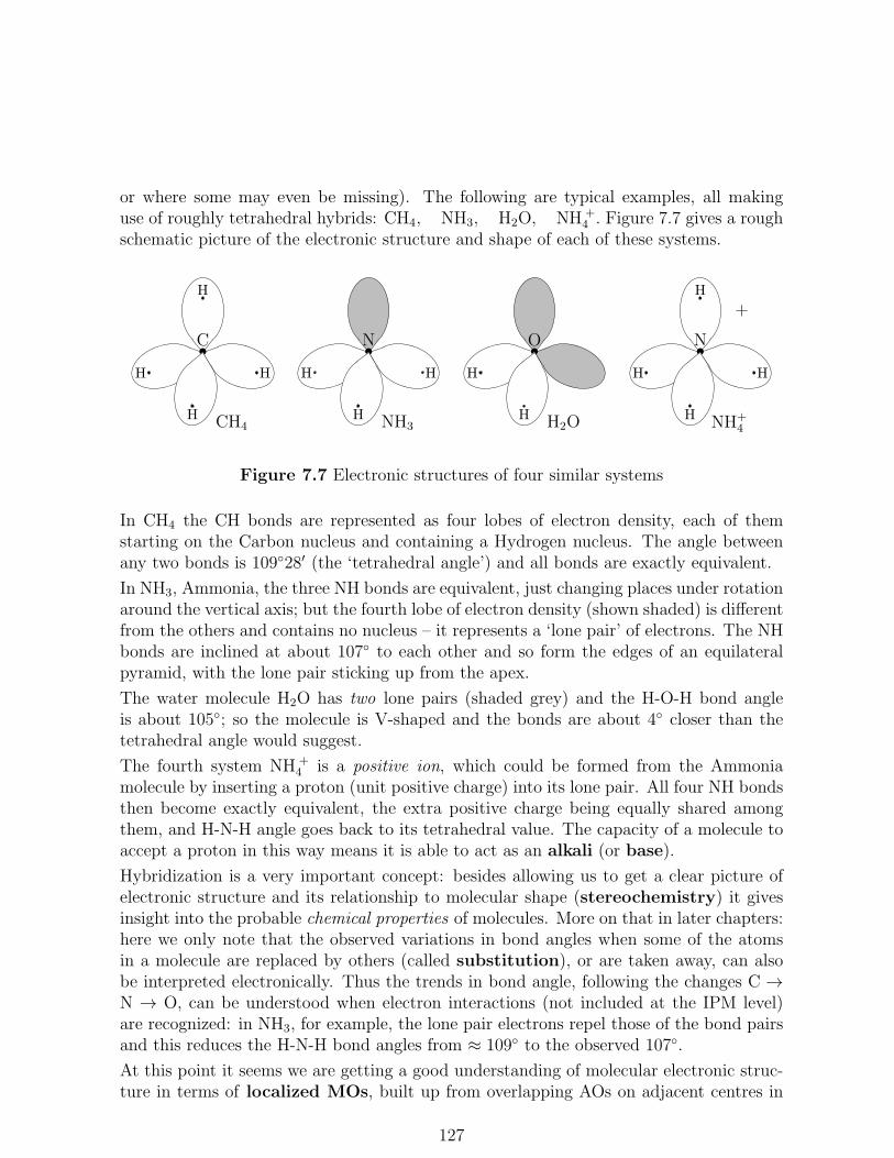
or where some may even be missing). The following are typical examples, all makinguse of roughly tetrahedral hybrids: CH4, NH3, H2O, NH +

4 . Figure 7.7 gives a roughschematic picture of the electronic structure and shape of each of these systems.

H

HH

•

H

C

CH4

HH

•N

H NH3

H

•O

H H2O

H

HH

•

H

N

NH+4

+

Figure 7.7 Electronic structures of four similar systems

In CH4 the CH bonds are represented as four lobes of electron density, each of themstarting on the Carbon nucleus and containing a Hydrogen nucleus. The angle betweenany two bonds is 109◦28′ (the ‘tetrahedral angle’) and all bonds are exactly equivalent.

In NH3, Ammonia, the three NH bonds are equivalent, just changing places under rotationaround the vertical axis; but the fourth lobe of electron density (shown shaded) is differentfrom the others and contains no nucleus – it represents a ‘lone pair’ of electrons. The NHbonds are inclined at about 107◦ to each other and so form the edges of an equilateralpyramid, with the lone pair sticking up from the apex.

The water molecule H2O has two lone pairs (shaded grey) and the H-O-H bond angleis about 105◦; so the molecule is V-shaped and the bonds are about 4◦ closer than thetetrahedral angle would suggest.

The fourth system NH +4 is a positive ion, which could be formed from the Ammonia

molecule by inserting a proton (unit positive charge) into its lone pair. All four NH bondsthen become exactly equivalent, the extra positive charge being equally shared amongthem, and H-N-H angle goes back to its tetrahedral value. The capacity of a molecule toaccept a proton in this way means it is able to act as an alkali (or base).

Hybridization is a very important concept: besides allowing us to get a clear picture ofelectronic structure and its relationship to molecular shape (stereochemistry) it givesinsight into the probable chemical properties of molecules. More on that in later chapters:here we only note that the observed variations in bond angles when some of the atomsin a molecule are replaced by others (called substitution), or are taken away, can alsobe interpreted electronically. Thus the trends in bond angle, following the changes C →N → O, can be understood when electron interactions (not included at the IPM level)are recognized: in NH3, for example, the lone pair electrons repel those of the bond pairsand this reduces the H-N-H bond angles from ≈ 109◦ to the observed 107◦.

At this point it seems we are getting a good understanding of molecular electronic struc-ture in terms of localized MOs, built up from overlapping AOs on adjacent centres in

127

the molecule. But we started from a much more complete picture in the general theory ofChapter 4, where every orbital was constructed, in principle, from a set of AOs centred onall the nuclei in the molecule. In that case the MOs of an IPM approximation of LCAOform would extend over the whole system: they would come out of the SCF calculationas completely nonlocalized MOs. We must try to resolve this conflict.

7.4 Why can we do so well with localized MOs?

That’s a good question, because Chapter 4 (on the Hartree-Fock method) made it seemthat a full quantum mechanical calculation of molecular electronic structure would bealmost impossible to do – even with the help of big modern computers. And yet, startingfrom a 2-electron system and using very primitive ideas and approximations, we’ve beenable to get a general picture of the charge distribution in a many-electron molecule andof how it holds the component atoms together.

So let’s end this section by showing how “simple MO theory”, based on localized orbitals,can come out from the quantum mechanics of many-electron systems. We‘ll start fromthe Hartree-Fock equation (4.12) which determines the ‘best possible’ MOs of LCAOform, remembering that this arises in IPM approximation from a single antisymmetrizedproduct of spin-orbitals:

ΨSCF =√N !A[ψ1(x1)ψ2(x2) ...ψN(xN). (7.7)

With the usual notation the spin-orbitals for a 10-electron system, such as the watermolecule, are

ψ1(x1) = φ1(r1)α(s1), ψ2(x2) = φ1(r2)β(s2), .... ψ5(x10) = φ5(r10)β(s10),

and the spatial functions are normally taken to be mutually orthogonal.

We know that this many-electron wave function leads to the 1-electron density function(spin included)

ρ(x1) = ψ1(x1)ψ∗1(x1) + ψ2(x1)ψ

∗2(x1) + ....+ ψN(x1)ψ

∗N(x1) (7.8)

and that for a closed-shell ground state the spin dependence can be removed by integrationto give the ordinary electron density

P (r1) = 2[φ1(r1)φ∗1(r1) + φ2(r1)φ

∗2(r1) + .... + φ5(r1)φ

∗5(r1)]

– a sum of orbital densities, times 2 as up-spin and down-spin functions give the samecontributions.

The spinless density matrix (see Chapter 5; and (5.33) for a summary) is very similar:

P (r1; r′1) = 2[φ1(r1)φ

∗1(r

′1) + φ2(r1)φ

∗2(r

′1) + .... + φN(r1)φ

∗N(r

′1)] (7.9)

128

and gives the ordinary electron density on identifying the two variables, P (r1) = P (r1; r1).These density functions allow us to define the effective Hamiltonian F used in Hartree-Fock theory and also give us, in principle, all we need to know about chemical bondingand a wide range of molecular properties.

The question is now whether, by setting up new mixtures of the spatial orbitals, we canobtain alternative forms of the same densities, without disturbing their basic property ofdetermining the ‘best possible’ one-determinant wave function. To answer the question,we collect the equations in (4.12), for all the orbitals of a closed-shell system, into a singlematrix equation

Fφ = φǫ, (7.10)

where the orbitals are contained in the row matrix

φ = (φ1 φ2 .... φN/2)

and ǫ is a square matrix with the orbital energies ǫ1, ǫ2, ...., ǫN/2 as its diagonal elements,all others being zeros. (Check this out for a simple example with 3 orbitals!)

Now let’s set up new linear combinations of the orbitals φ1, φ2, ... φN/2, and collect themin the row matrix

φ = (φ1, φ2, ... φN/2).

The set of complex conjugate functions, φ∗i , is then written as a column, obtained by

transposing the row and putting the star on each of its elements – an operation indicatedby a ‘dagger’ (†). With these conventions, which you may remember from Chapter 4, thenew mixtures can be related to the old by the matrix equation

φ = φU (7.11)

where the square matrix U has elements Urs which are the ‘mixing coefficients’ givingφs =

∑

r φrUrs. The new density matrix can be expressed as the row-column matrixproduct

P (r1; r′1) = φ φ

†

and is then related to that before the transformation, using (7.11), by

P (r1; r′1) = φU(φU)†

= φU(U†φ†)

= P (r1; r′1) (provided UU† = 1. (7.12)

Here we’ve noted that (AB)† = (B†A†) and the condition on the last line means that Uis a unitary matrix.

That was quite a lot of heavy mathematics, but if you found it tough go to a real appli-cation in the next Example, where we relate the descriptions of the water molecule basedon localized and non-localized MOs. You should find it much easier.

129

Example 7.5 Transformation from localized to non-localized orbitals: H2O

To show what the matrix U looks like let’s use (7.11) to pass from the basis of localized orbitals φ, whichwe set up by intuition (‘guess work’), to non-localized orbitals similar to those that come from an SCFcalculation – putting them in the row matrix φ.

To do that we need to express (7.11) the other way round, but that’s easy because when both orbitalsets are orthonormal (as we suppose) U will be unitary, UU† = 1. So multiplying from the right by U†

gives φU† = φ.

We want to choose U†, then, so that the orbitals in φ are completely de-localized over the whole molecule;and we know that these orbitals will be of various types as a result of molecular symmetry. Some will besymmetric under a reflection that interchanges left and right, others will be anti-symmetric – changingonly in sign – and so on.

In Figure 7.4 the H2O molecule is inscribed in a cube, for comparison with the other systems, and hereit’s convenient to use the same figure. The atoms of H1–O–H2 then lie in the xz-plane, with O as originand z-axis pointing upwards (above the H atoms). This plane is a symmetry plane, the molecule beingsymmetric under reflection across it; but the xy-plane is a second plane of symmetry, across which theH atoms simply change places under reflection. The two reflections are both symmetry operations,which leave the system apparently unchanged. Another kind of symmetry operation may be a rotation,like that of half a turn (through 180◦) about the z-axis – which also interchanges the H atoms. Thesethree operations are usually denoted by σ1, σ2 for the reflections and C2 for the rotation; together withthe “identity operation” E (do nothing!) they form the symmetry group of the system. (If you’veforgotten about such things,turn back to Chapter 7 of Book 11 – or even to Chapter 6 of Book 1 !)

The localized orbitals we have in mind for the water molecule were constructed from the valence hybridsh1, h2 overlapping with the Hydrogen 1s AOs (let’s call them H1 and H2) to give two bond orbitals

φ1 = ah1 + bH1, φ2 = ah2 + bH2.

Here the bonds are equivalent, so the mixing coefficients a, b must be the same for both of them. Theremaining 4 of the 8 valence electrons represent two lone pairs and were assigned to the next two hybridsh3 and h4, which we may now denote by

φ3 = h3 and φ4 = h4.

What about the non-localized MOs? These will be put in the row matrix φ = (φ1 φ2 φ3 φ4) and shouldserve as approximations to the MOs that come from a full valence-electron SCF calculation. There areonly four occupied SCF orbitals, holding the 8 valence electrons, and for a symmetrical system like H2Othey have simple symmetry properties. The simplest would be symmetric under rotation C2, through180◦ around the z-axis, and also under reflections σ1, σ2 across the xz- and yz-planes. How can we expresssuch orbitals in terms of the localized set φ ? Clearly φ1 and φ2 are both symmetric under reflection σ1across the plane of the molecule, but they change places under the rotation C2 and also under σ2 – whichinterchanges the H atoms. For such operations they are neither symmetric nor anti-symmetric; and thesame is true of φ3 and φ4. However, the combination φ1 + φ2 clearly will be fully symmetric. Reflectionsends the positive combination into itself, so φ1 + φ2 is symmetric, but φ1 − φ2 becomes φ2 − φ1 and istherefore anti-symmetric under C2 and σ2. Moreover, the symmetric and anti-symmetric combinationsare both delocalized over both bonds and can be used as

φ1 = (1/√2)(φ1 + φ2), φ2 = (1/

√2)(φ1 − φ2),

where we remembered that all orbitals are supposed to be orthonormal. Similarly, the localized andnon-localized lone-pair orbitals are related by

φ3 = (1/√2)(φ3 + φ4), φ4 = (1/

√2)(φ3 − φ4).

130

Finally, these results may be put in matrix form, φ = φU†, where the matrix U† is

U† =

x x 0 0x x 0 00 0 x x0 0 x x

(x and x standing for 12

√2 and − 1

2

√2.) It is easy to confirm that this matrix is unitary. Each column

contains the coefficients of a nonlocalized MO in terms of the four localized MOs; so the first expresses φ1

as the combination found above, namely (1/√2)(φ1 + φ2), while the fourth gives φ4 = (1/

√2)(φ3 − φ4).

In each case the sum of the coefficients squared is unity (normalization); and for two columns the sum of

corresponding products is zero (orthogonality).

In summary, Example 7.5 has shown that

φ1 = (1/√2)(φ1 + φ2) and φ2 = (1/

√2)(φ1 − φ2) (7.13)

are delocalized combinations of localized bond orbitals, behaving correctly under symme-try operations on the molecule and giving exactly the same description of the electrondistribution. The same is true of the lone pair orbitals: they may be taken in localizedform as, φ3 and φ4, which are clearly localized on different sides of a symmetry plane, orthey may be combined into the delocalized mixtures

φ3 = (1/√2)(φ3 + φ4) and φ4 = (1/

√2)(φ3 − φ4) (7.14)

The localized and non-localized orbital sets give entirely equivalent descriptions of theelectron distribution, provided they are related by a unitary transformation φ = φU†. Inthe case of the water molecule

U† =

x x 0 0x x 0 00 0 x x0 0 x x

, (7.15)

where x and x stand for the numerical coefficients 12

√2 and −1

2

√2. Thus, for example, the

localized lone pairs are φ3 = h3 and φ4 = h4, and their contribution to the total electrondensity P is 2|h3|2 + 2|h4|2 (two electrons in each orbital).

After transformation to the delocalized combinations, given in (7.14), the density contri-bution of the lone pairs is expressed as (Note that the ‘square modulus’ |...| is used as theelectron density P is a real quantity, while the functions may be complex.)

2|φ3|2 + 2|φ4|2 = |(h3 + h4)|2 + |(h3 − h4)|2= (|h3|2 + |h4|2 + 2|h3h4|) + (|h3|2 + |h4|2 − 2|h3h4|)= 2|h3|2 + 2|h4|2

– exactly as it was before the change to non-localized MOs.

131

You can write these results in terms of the usual s, px, py, pz AOs (you should try it!),getting

φ3 =√2(s + pz), φ4 =

√2(px + py).

Evidently, |φ3|2 describes a lone-pair density lying along the symmetry axis of the molecule(sticking out above the Oxygen) while |φ4|2 lies in the plane of the molecule and describesa ‘halo’ of negative charge around the O atom.

The water molecule provided a very simple example, but (7.14) and all that followsfrom it are quite general. Usually the transformation is used to pass from SCF MOs,obtained by solving the Hartree-Fock equations, to localized MOs, which give a muchclearer picture of molecular electronic structure. In that case (7.11) must be used, withsome suitable prescription to define the matrix U that will give maximum localization

of the transformed orbitals. Many such prescriptions exist and may be applied even whenthere is no symmetry to guide us, as was the case in Example 7.5: they provide a usefullink between Quantum Mechanics and Chemistry.

7.5 More Quantum Chemistry

– the semi-empirical treatment of bigger molecules

At IPM level, we’ve already explored the use of Molecular Orbital (MO) theory intrying to understand the electronic structures of some simple molecules formed fromatoms of the First Row of the Periodic Table, which starts with Lithium (3 electrons) andends with Neon (10 electrons).

Going along the Row, from left to right, and filling the available AOs (with up to twoelectrons in each) we obtain a complete ‘shell’. We made a lot of progress for diatomic

molecules (homonuclear when both atoms are the same, heteronuclear when they aredifferent) and even for a few bigger molecules, containing 3,4, or more atoms. After findingthe forms of rough approximations to the first few MOs we were able to make pictures

of the molecular electronic structures formed by adding electrons, up to two at a time,to the ‘empty’ MOs. And, remember, these should really be solutions of the Schrodingerequation for one electron in the field provided by the nuclei and all other electrons: theyare not ‘buckets’ for holding electrons! – they are mathematical functions with sizes andshapes, like the AOs used in Section ... to describe the regions of space in which theelectron is most likely to be found.

In the approach used so far, the MOs that describe the possible stationary states of anelectron were approximated as Linear Combinations of Atomic Orbitals on theseparate atoms of the molecule (the LCAO approximation). On writing

φ = c1χ1 + c2χ2 + ... cnχn =∑

i

ciχi, (7.16)

the best approximations we can get are determined by solving a set of secular equations.

132

In the simple case n = 3 these have the form (see equation (4.15) of Section 4)

h11 h12 h13h21 h22 h23h31 h32 h13

c1c2c3

= ǫ

c1c2c3

. (7.17)

In Section 4 we were thinking about a much more refined many-electron approach, withas many basis functions as we wished, and an effective Hamiltonian F in place of the‘bare nuclear’ operator h. The Fock operator F includes terms which represent interactionwith all the other electrons, but here we use a strictly 1-electron model which containsonly interaction with the nuclei. The matrix elements hij are then usually treated asdisposable parameters, whose values are chosen by fitting the results to get agreementwith any available experimetal data. And the overlap integrals Sij = 〈χi|χj〉 are oftenneglected for i 6= j. This is the basis of semi-empirical MO theory, which we explorefurther in this section.

Let’s start by looking at some simple hydrocarbons, molecules that contain only Carbonand Hydrogen atoms, beginning with Acetylene (C2H2) – the linear molecule H − C ≡C−H, studied in Example 7.3, where the simplest picture of the electronic structure wasfound to be

φ 2CHφ

2CCσzφ

2CCπxφ

2CCπyφ

2CH.

That means, you’ll remember, that two electrons occupy the MO φCH localized aroundthe left-hand CH bond; another two occupy φCCσz, a σ-type MO localized around the C–C(z) axis; two more occupy a π-type MO φCCπx formed from 2px AOs; two more occupya similar MO φCCπy formed from 2py AOs; and finally there are two electrons in theright-hand CH bond. That accounts for all 10 valence electrons! (2 from the Hydrogensand 2×4 from the Carbons) And in this case the localized MOs are constructed from thesame number of AOs.

Now suppose the MOs came out from an approximate SCF calculation as general linearcombinations of the 10 AOs, obtained by solving secular equations like () but with 10 rowsand columns. What form would the equations have? The matrix elements hij for pairsof AOs χi, χj would take values hii = αi, say, along the diagonal (j = i); and this wouldrepresent the expectation value of the effective Hamiltonian h for an electron sitting in χi.(This used to be called a “Coulomb” integral, arising from the electrostatic interactionwith all the nuclei.) The off-diagonal elements hij, (j 6= i) would arise jointly from theway χi and χj ‘overlap’ (not the overlap integral, which we have supposed ‘negligible’).It is usually denoted by βij and is often referred to as a ‘resonance’ integral because itdetermines how easily the electron can ‘resonate’ between one AO and the other. Insemi-empirical work the αs and βs are looked at as the ‘disposable parameters’ referredto above.

In dealing with hydrocarbons the αs may be given a common value αC for a Carbonvalence AO αH for a Hydrogen AO. The βs are given values which are large for AOs witha heavy overlap (e.g. hybrids pointing directly towards each other), but are otherwise

133

neglected (i.e. given the value zero). This is the nearest-neighbour approximation.To see how it works out let’s take again the case of Acetylene.

Example 7.6 Acetylene – with 10 AOs

Choose the AOs as the hybrids used in Example 7.3. Those with σ symmetry around the (z) axis of themolecule are:

•χ1 = left-hand Hydrogen 1s AO

•χ2 = Carbon σ hybrid pointing towards Hydrogen (χ1)

•χ3 = Carbon σ hybrid pointing towards second Carbon (χ4)

•χ4 = Carbon σ hybrid pointing towards first Carbon (χ3)

•χ5 = Carbon σ hybrid pointing towards right-hand Hydrogen

•χ6 = right-hand Hydrogen 1s AO

The other Carbon hybrids are of x-type, formed by including a 2px component, and y-type, formed byincluding a 2py component. They are

•χ7 = x-type hybrid on first Carbon, pointing towards second

•χ8 = x-type hybrid on second Carbon, pointing towards first

•χ9 = y-type hybrid on first Carbon, pointing towards second

•χ10 =y-type hybrid on second Carbon, pointing towards first

You should draw pictures of all these hybrid combinations and decide which pairs will overlap to give

non-zero βs.

To determine the form of the secular equations we have to decide which AOs are ‘nearestneighbours’, so let’s make a very simple diagram in which the AOs χ1, ... χ10 are indicatedby short arrows showing the way they ‘point’ (usually being hybrids). As the molecule islinear, the arrows will be arranged on a straight line as in Figure 7.8 below:

•H

•C

•C

•H

χ1 χ2 χ3 χ4 χ5 χ6

χ7 χ8

χ9 χ10

Figure 7.8 Overlapping orbital pairs in C2H2

From the Figure, the diagonal elements in the matrix of the 1-electron Hamiltonian, h,will be hii = 〈χi|h|χi〉; so

h11 = αH, h22 = h33 = h44 = h55 = αC, h66 = αH,

(all with σ symmetry around the z-axis) and, if we take all the Carbon hybrids as ap-proximately equivalent,

h77 = h88 = h99 = h10,10 = αC.

h77 = h88 = h99 = h10,10 = αC.

134

The off-diagonal elements hij = 〈χi|h|χj〉 will be neglected, in nearest-neighbour approx-imation, except for χiχj pairs that point towards each other. The pairs (1,2) and (5,6)may be given a common value denoted by βCH, while (3,4),(7,8),(9,10) may be given acommon value βCC. For short, we’ll use just β for the C-C resonance integral and β′ forthe one that links C to H.

Since i and j are row- and column- labels of elements in the matrix h, it follows that theapproximate form of h for the Acetylene molecule is

α′ β′ 0 0 0 0 0 0 0 0β′ α 0 0 0 0 0 0 0 00 0 α β 0 0 0 0 0 00 0 β α 0 0 0 0 0 00 0 0 0 α β′ 0 0 0 00 0 0 0 β′ α′ 0 0 0 00 0 0 0 0 0 α β 0 00 0 0 0 0 0 β α 0 00 0 0 0 0 0 0 0 α β0 0 0 0 0 0 0 0 β α

(7.18)

The secular equations contained in the matrix hc = ǫc then break up into pairs, corre-sponding to the 2×2 ‘blocks’ along the diagonal of (7.18). The first pair, for example,could be written

(α′ − ǫ)c1 + β′c2 = 0, β′c1 + (α− ǫ)c2 = 0

and the solution is easy (you’ve done it many times before!): by ‘cross-multiplying’ youeliminate the coefficients and get

(α′ − ǫ)(α− ǫ)− (β′)2 = 0,

which is a simple quadratic equation to determine the two values of ǫ for which the twoequations can be solved (are ‘compatible’). These values, the ‘roots’, are (look back atSection 5.3 of Book 1 if you need to!)

ǫ = 12(α + α′)± 1

2

√

(α− α′)2 + 4(β′)2). (7.19)

Since the αs and βs are all negative quantities (do you remember why?) the lowest rootwill be ǫ1 = 1

2− 1

2

√

(α + α′)2 + 4(β′)2 and this will be the orbital energy of an electronin the localized MO describing the CH bond. To get the form of this bonding MO allyou have to do is substitute ǫ = ǫ1 in either of the two equations leading to (8.4): thiswill determine the ratio of the coefficients and their absolute values then follow from thenormalization condition c 21 +c

22 = 1. This has been done in detail for some simple diatomic

molecules in Section 6.2, which you may want to read again.

All the localized MOs follow in exactly the same way from the other diagonal blocks in(7.18). For the bonds involving similar AOs the equations contain no ‘primed’ quantities

135

and (7.19) gives ǫ1 = α + β, ǫ2 = α − β for the bonding and antibonding combinations.In that case the corresponding normalized MOs are

Bonding : φ1 = (χ1 + χ2)/√2, Antibonding : φ2 = (χ1 − χ2)/

√2, (7.20)

just as for a homonuclear diatomic molecule (Section 7.2). In other words the IPMpicture, with nearest-neighbour approximations, views the molecule as a superpositionof independent 2-electron bonds, each one consisting of two electrons in a localized MOextending over only two centres. In this extreme form of the IPM approximation, thetotal electronic energy is represented as a sum

Etotal ≈∑

rs(pairs)

E(rs), (7.21)

where E(rs) = 2ǫ(rs) and is the energy of two electrons in the bonding MO formed froman overlapping pair of AOs χr, χs.

The total electronic energy of the Acetylene molecule would thus be

Etotal ≈ 2ECH + 3ECC

– corresponding to 2 CH bonds and 3 CC bonds (taken as being equivalent).

From Acetylene to Ethane and Ethylene

In Acetylene the Carbons, which are each able to form bonds with up to four other atoms(as in Methane, CH4, shown in Figure 7.7), are each bonded with only one other atom.The CC triple bond seems a bit strange, with each Carbon using 3 of its 4 valencies toconnect it only with another Carbon! – and the triple bond is apparently quite differentfrom that in the diatomic Nitrogen molecule N ≡ N, described in Section 7.2 as onebond of σ type with two somewhat weaker π-type bonds. Instead we’ve described it interms of hybrid AOs, one pair (χ3, χ4), pointing directly towards each other, and twopairs pointing away from the molecular axis and able to form only ‘bent’ bonds. In fact,however, both descriptions are acceptable when we remember that the hybrid AOs aresimply linear combinations of 2s and 2p AOs and the three pairs of localized MOs formedby overlapping the hybrids are just alternative combinations. In Section 7.4 we foundhow two alternative sets of orbitals could lead to exactly the same total electron density,provided the mixing coefficients were chosen correctly so as to preserve normalization andorthogonality conditions. So don’t worry! – you can use either type of MOs and get moreor less the same overall description of the electronic structure. Any small differences willarise from using one set of ‘standard’ s-p hybrids in a whole series of slightly differentmolecular situations (as in Figure 7.7).

Ethane and Ethylene illustrate two main categories of carbon compounds: in Ethanethe Carbon forms four σ-type bonds with other atoms (we say all carbon valencies aresaturated), leading to “saturated molecules”; but in Ethylene only three carbon valenciesare used in that way, the fourth being involved in somewhat weaker π-type bonding, and

136

Ethylene is described as an “unsaturated molecule”. Let’s deal first with Ethane andsimilar molecules.

The Ethane molecule

Ethane has the formula C2H6, and looks like two CH3 groups with a σ bond between thetwo Carbons. Its geometry is indicated in Figure 7.9 below:

•C •C

H

H

H

H

H

H

Figure 7.9 Geometry of the Ethane molecule

Here the molecule is shown sitting inside a rectangular box (indicated by the light bluebroken lines) so you can see its 3-dimensional form. Each Carbon uses one of its fourhybrids to make a sigma bond with the other Carbon, while its three remaining hybridsconnect it with Hydrogens. The right-hand CH3 group is rotated around the C−C axis,relative to the CH3 on the left; this is called the “staggered conformation” of the molecule.The energy variation in such a rotation is a tiny fraction of the total electronic energy;in the “eclipsed conformation”, where each group is the mirror image of the other acrossa plane perpendicular to the C−C axis, cutting the molecule in two, the total energy isabout 12 kJ/mol higher – but this is less than (1/20,000)th of the total energy itself!The energy difference between the two conformations is a rotational ‘barrier height’ butis clearly much too small to be predicted with the crude approximations we are using.In IPM approximation with inclusion of only nearest neighbour interactions the totalelectronic energy for either conformation would be simply

Etotal ≈ 6ECH + ECC

and this does not depend on rotation of one group relative to the other. (To be remindedof energy units go back to Book 5, Section 3.1)

Ethane is the second member of the series starting with methane, often called theParaffin

series. The next one is Propane C3H8, formed by adding another CH2 group between thetwo Carbons in Ethane. Because there is so little resistence to twisting around a C−Csingle bond, such chains are very flexible. They are also chemically stable, not reactingeasily with other molecules as all valencies are saturated. Members of the series with theshortest chains form gases, becoming liquids as the chain length increases (e.g. gasolene

137

with 7-9 Carbons and kerosene with 10-16 Carbons) and finally solid paraffin. Obviouslythey are very important commercially.

The Ethylene molecule

In this molecule, with the formula C2H4, each Carbon is connected to only two Hydrogensand the geometry of the molecule is indicated in Figure 7.10 here two CH2 groups lie in thesame plane (that of the paper) and are connected by a C−C sigma bond. Each Carbonhas three valencies engaged in sigma-bonding; the fourth involving the remaining 2p AO,sticking up normal to the plane of the molecule and able to take part in π bonding.

. .• •C C

H H

H H

Figure 7.10 Geometry of Ethylene

Molecules with Carbons of this kind are said to be “conjugated” and conjugated molecules

form an important part of carbon chemistry. The Ethylene molecule is flat, with Carbon2p orbitals normal to the plane and overlapping to give a π bond; there is thus a CC dou-ble bond, which keeps the molecule flat, because twisting it around the CC bond reducesthe lateral overlap of the 2p orbitals and hence the degree of π bonding. Unsaturatedhydrocarbons like Ethylene are generally planar for the same reason. They can all be

built up by replacing one of the Hydrogens by a trivalent Carbon .• and saturatingtwo of the extra valencies by adding two more Hydrogens. From Ethylene we obtain inthis way C3H6 (The Allyl radical), which has 3 π electrons and is a highly reactive “freeradical”.

The Butadiene molecule

On replacing the right-most Hydrogen of Allyl by another CH2 group, we obtain themolecule pictured in Figure 7.11 which is called “Butadiene”:

. .

. .

•C •C

•C •CH

H H

H H

H

Figure 7.11 The Butadiene molecule

As you can see, the chain of Carbons is not straight but ‘zig-zag’ – as a result of thetrigonal symmetry of the electron distribution around each Carbon. But, if we thinkabout the π electrons alone – as if they moved in the field of a ‘rigid framework’ providedby the σ-bonded atoms – that’s not important: in a nearest-neighbour approximation all

138

that matters is the pattern of connections due to lateral overlap of 2p AOs on adjacentCarbons. In the early applications of quantum mechanics to molecules this approximationturned up an amazing number of chemically important results. So let’s use Butadiene totest our theoretical approach:

Example 7.7 Butadiene: electronic structure of the π-electron system

In the present approximation we think only of the C−C−C−C chain and set up the secular equationsfor a π electron in the field of the σ-bonded framework. The effective Hamiltonian has diagonal matrixelements α for every Carbon and off-diagonal elements β for every pair of nearest neighbours, the restbeing neglected. The equations we need are therefore (check it out!)

α− ǫ β 0 0β α− ǫ β 00 β α− ǫ β0 0 β α− ǫ

c1c2c3c4

=

0000

There are solutions only for values of ǫ which make the determinant of the square matrix zero. How canwe find them?

The first line of the matrix equation above reads as

(α− ǫ)c1 + βc2 = 0

and it would look better if you could get rid of the α and β, which are just parameters that can takeany values you choose. So why not divide all terms by β, which doesn’t change anything, and denote(α− ǫ)/β by −x? The first equation then becomes −xc1+c2 = 0 and the whole matrix equation becomes

−x 1 0 01 −x 1 00 1 −x 10 0 1 −x

c1c2c3c4

=

0000

There are solutions only for values of x which make the determinant of the square matrix zero; and ifyou know how to solve for x you can get all the energy levels for any values of the adjustable parametersα, β.

The equation to determine the acceptable values of x is thus∣

∣

∣

∣

∣

∣

∣

∣

−x 1 0 01 −x 1 00 1 −x 10 0 1 −x

∣

∣

∣

∣

∣

∣

∣

∣

= 0 (7.22)

You may remember the rule for evaluating a determinant (it was given first just afterequation (6.10) in Book 2). Here we’ll use it to evaluate the 4×4 determinant of thesquare matrix on the left in (7.22). Working along the first row and denoting the valueof the 4×4 determinant by ∆4(x) (it’s a function of x) we get in the first step

∆4(x) =

∣

∣

∣

∣

∣

∣

∣

∣

−x 1 0 01 −x 1 00 1 −x 10 0 1 −x

∣

∣

∣

∣

∣

∣

∣

∣

= (−x)

∣

∣

∣

∣

∣

∣

−x 1 01 −x 10 1 −x

∣

∣

∣

∣

∣

∣

− (1)

∣

∣

∣

∣

∣

∣

1 1 00 −x 10 1 −x

∣

∣

∣

∣

∣

∣

+ etc.

139

The next step is to use the same rule to evaluate each of the 3×3 determinants. You’llneed only the first two as the others are multiplied by zero. The first one is

∣

∣

∣

∣

∣

∣

−x 1 01 −x 10 1 −x

∣

∣

∣

∣

∣

∣

= (−x)∣

∣

∣

∣

−x 11 −x

∣

∣

∣

∣

− (1)

∣

∣

∣

∣

1 10 −x

∣

∣

∣

∣

+ (0)

∣

∣

∣

∣

1 −x0 1

∣

∣

∣

∣

The second one is∣

∣

∣

∣

∣

∣

1 1 00 −x 10 1 −x

∣

∣

∣

∣

∣

∣

= (1)

∣

∣

∣

∣

−x 11 −x

∣

∣

∣

∣

– the other 2×2 determinants being multiplied by zeros.

Any 2×2 determinant∣

∣

∣

∣

a bc d

∣

∣

∣

∣

= ad− cb

– as follows from the rule you’re using (check it) and it’s therefore easy to work backfrom this point and so evaluate the original 4×4 determinant ∆4(x). The final result is(check it!) ∆4(x) = x4 − 3x2 + 1 and depends only on the square of x. That shows atonce that the set of energy levels will be symmetrical around x = 0; and if we put x2 = ythe consistency condition ∆4(x) = 0 becomes y2 − 3y + 1 = 0. This simple quadraticequation has roots y = (3 ±

√5)/2, which lead to x = ±

√

(1.618), or x = ±√

(0.618);and therefore to energy levels

ǫ = α± xβ = α± 1.272β, or α± 0.786β.

Since α and β are both negative quantities the level for the plus sign is below the ‘datum’ αand corresponds to a ‘bonding’ state, while that with the negative sign lies symmetricallyabove the datum and corresponds to an ‘antibonding’ state.

The calculation above, for a chain of four Carbons, could be repeated for a chain of sixCarbons (called “Hexatriene”) but would involve dealing with a 6×6 determinant; andwith N Carbons we would have to deal with an N × N determinant – quite a lot ofwork! Sometimes, however, it is simpler to solve the simultaneous equations directly: themethod is shown in Example 7.8 that follows.

Example 7.8 Butadiene: a simpler and more general method

Again we calculate the electronic structure of the π-electron system of Butadiene, but this time we workdirectly from the secular equations, which follow from (7.22) as

(α− ǫ)c1 + βc2 + 0c3 + 0c4 = 0c1

βc1 + (α− ǫ)c2 + βc3 + 0c4 = 0c2

0c1 + βc2 + (α− ǫ)c3 + βc4 = 0c3

0c1 + 0c2 + βc3 + (α− ǫ)c4 = 0c4,

140

where the sum of terms on the left of the equality must vanish for every line. In short,

(α− ǫ)c1 + βc2 = 0, βc1 + (α− ǫ)c2 + βc3 = 0, βc2 + (α− ǫ)c3 + βc4 = 0, βc3 + (α− ǫ)c4 = 0.

Let’s now write cm for the mth coefficient (in the order 1,2,3,4), divide each equation by β, and againput (α− ǫ)/β = −x. The whole set of equations can then be written as a single one:

cm−1 − xcm + cm+1 = 0,

where m takes the values 1,2,3 and 4 in turn and we exclude any values such as 0 or 5 that lie outsidethat range. These are ‘boundary conditions’ which tell us there are no coefficients below m=1 or abovem=4. The number of atoms in the chain (call it N) is not important as long as we insist that c0 andcN+1 should be zero. So now we can deal with polyene chains of any length!

To complete the calculation we can guess that the coefficients will follow the up-and-down pattern ofwaves on a string, like the wave functions of an electron in a 1-dimensional box – behaving like sinmθ orcosmθ or a combination of the two. It’s convenient to use the complex forms exp(±)imθ and on puttingcm = exp(imθ) in the key equation above we get the condition

exp i(m− 1)θ − x exp mθ + exp i(m+ 1)θ = 0.

Taking out a common factor of exp imθ, this gives eiθ + e−iθ − x = 0, so the ‘wavelength’ θ must berelated to the energy x by x = 2 cos θ.

Since changing the sign of m gives a solution of the same energy, a more general solution will be

cm = A exp(imθ) +B exp(−imθ)

where A and B are arbitrary constants, which must be chosen to satisfy the boundary conditions: thefirst of these, c0 = A+B = 0, gives

cm = A[exp(imθ)− exp(−imθ)] = C sin(mθ), (C = 2A)

while the second, taking m = N + 1, becomes

cN+1 = C sin (N + 1)θ = 0.

This is satisfied only when (N + 1)θ = kπ where k is any positive integer and is essentially a quantum

number for the kth state of the system. The wavelength in the kth state is thus θ = kπ/(N + 1); so theMO φk will be φk =

∑

cmχm with AO coefficient cm = C sin mkπ/(N + 1) and will have correspondingorbital energy xk = C cos(kπ/(N + 1).

From Example 7.8, the MOs φk for a polyene chain of N Carbons are φk =∑

c(k)m χm,

where the mth AO coefficient is (after normalizing – check it!)

c(k)m = Ck sin

(

mkπ

N + 1

)

(Ck =√

2/(N + 1)). (7.23)

The corresponding orbital energies are ǫk = α + βxk, with

xk = 2 cos

(

kπ

N + 1

)

. (7.24)

The energy levels are thus symmetrically disposed around ǫ = α, which may be taken asa reference level. As N → ∞ the levels become closer and closer, eventually forming a

141

continuous energy band extending from ǫ = α+ 2β up to α− 2β. (Remember α and βare both negative.) All this is shown below in Figure 7.12.

It should be noted that when the number of Carbons is odd there is always a Non-bonding MO: it is very important, giving the molecule its ‘free-radical’ character – thehighest occupied orbital leading to a highly reactive system with a very short lifetime.

N = 1 N = 2 N = 3 N = 4 N →∞

← Non-bonding

l Anti-bonding

l Bonding

Figure 7.12 MO energy levels in a chain of N Carbon atoms

The reference level (N = 1) in Figure 7.12 has ǫ = α. As N →∞ the levels become veryclose, forming an energy band extending from ǫ = α + 2β up to α− 2β. (Remember αand β are both negative.) It should be noted that when the number of Carbons is oddthere is always a Non-bonding MO: it is very important, giving the molecule its ‘free-radical’ character – the highest occupied orbital leading to a highly reactive system witha very short lifetime.

It is also interesting to ask what happens if you join the ends of a chain molecule to forma ring – a ‘cyclic’ molecule. In Example 7.9 we find the question is easily answered bymaking a simple change of the boundary conditions used in Example 7.8.

Example 7.9 Making rings – cyclic polyenes

If we join the ends of a chain of N Carbons, keeping the system flat with adjacent atoms connected bystrong σ bonds, we obtain a ring molecule in which every Carbon provides one π electron in a 2p AOnormal to the plane. In nearest neighbour approximation, the equations to determine the MO coefficientsare unchanged – except that the AOs χ1 and χN will become neighbours, so there will be a new non-zeroelement in the first and last rows of the matrix h. For a 6-Carbon ring, called Benzene, h16 and h61 willboth have the value β instead of zero. The secular equations will then become

(α− ǫ)c1 + βc2 + βc6 = 0,

βc1 + (α− ǫ)c2 + βc3 = 0,

βc2 + (α− ǫ)c3 + βc4 = 0,

βc3 + (α− ǫ)c4 + βc5 = 0,

βc4 + (α− ǫ)c5 + βc6 = 0,

βc1 + βc5 + (α− ǫ)c6 = 0,

where the terms at the end of the first line and the beginning of the last line are ‘new’: they arise becausenow the Carbon with AO cofficient c1 is connected to that with AO coefficient c6.

142

On putting (α − ǫ)/β = −x, as before, and dividing throughout by β, the first and last of the secularequations become, respectively,

−xc1 + c2 + c6 = 0 and c1 + c5 − xc6 = 0,

but all the other equations have the ‘standard’ form

cm−1 − xcm + cm+1 = 0

with m taking values 2, 3, 4, 5. The first equation does not fit this pattern because, putting m = 1, itwould need a term c0 – which is missing. The last equation also does not fit – because with m = 6 itwould need a term c7, which is also missing.

To get round this problem we use a simple trick. We allow them to exist but make a change of inter-pretation: on counting round the ring in the direction of increasing m we note that m = 6 + 1 brings usback to the seventh atom, which coincides with the first – so c7 = c1 and c8 = c2 etc. – and in generalcm+N = cm for a ring of N atoms. This is called a periodic boundary condition and on puttingcm = exp(imθ), as before, we must now require that exp(imθ) = exp i(m+N)θ.

The acceptable values of θ are thus limited to the solutions of exp(iNθ) = 1, which are θ = 2πk/N, wherek is an integer (positive, negative, or zero). The MOs and their energies are thus determined in generalby

c(k)m = Ak exp(2πimk/N), xk = 2 cos(2πk/N) (k = 0,±1,±2,±3).

To summarize what came out from Example 7.9, joining the ends of a long polyene chain toform a ring leaves the formula for the energy levels, namely (7.24), more or less unchanged–

ǫk = α + 2β cos

(

2πk

N

)

(7.25)

– with N instead of N + 1, but gives a complex MO with AO coefficients

c(k)m = Ak exp

(

2πimk

N

)

(Ak = 1/√N). (7.26)

However, changing the sign of k in (7.24) makes no difference to the energy, so the solutionsin (7.26) can be combined in pairs to give real MOs with AO coefficients

a(k)m = Ck sin

(

2πmk

N

)

, b(k)m = Ck cos

(

2πmk

N

)

,

where Ck is again chosen to normalize the function. On putting N = 6, for example, thethree bonding π-type MOs for the Benzene molecule can be written as

φ1 = (1/√6)(χ1 + χ2 + χ3 + χ4 + χ5 + χ6)

φ2 = −(1/2√3)(χ1 + 2χ2 + χ3 − χ4 − 2χ5 − χ6)

φ3 = (1/2)(χ1 − χ3 − χ4 − 2χ5 + χ6). (7.27)

The molecule forms a sweet-smelling liquid of great importance in the chemical industry.It is used in the manufacture of drugs, dyes, plastics and even explosives and is the first in

143

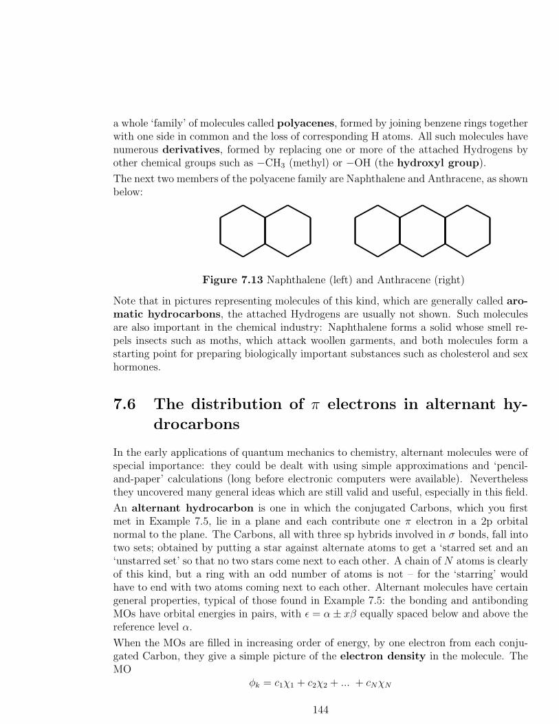
a whole ‘family’ of molecules called polyacenes, formed by joining benzene rings togetherwith one side in common and the loss of corresponding H atoms. All such molecules havenumerous derivatives, formed by replacing one or more of the attached Hydrogens byother chemical groups such as −CH3 (methyl) or −OH (the hydroxyl group).

The next two members of the polyacene family are Naphthalene and Anthracene, as shownbelow:

Figure 7.13 Naphthalene (left) and Anthracene (right)

Note that in pictures representing molecules of this kind, which are generally called aro-

matic hydrocarbons, the attached Hydrogens are usually not shown. Such moleculesare also important in the chemical industry: Naphthalene forms a solid whose smell re-pels insects such as moths, which attack woollen garments, and both molecules form astarting point for preparing biologically important substances such as cholesterol and sexhormones.

7.6 The distribution of π electrons in alternant hy-

drocarbons

In the early applications of quantum mechanics to chemistry, alternant molecules were ofspecial importance: they could be dealt with using simple approximations and ‘pencil-and-paper’ calculations (long before electronic computers were available). Neverthelessthey uncovered many general ideas which are still valid and useful, especially in this field.

An alternant hydrocarbon is one in which the conjugated Carbons, which you firstmet in Example 7.5, lie in a plane and each contribute one π electron in a 2p orbitalnormal to the plane. The Carbons, all with three sp hybrids involved in σ bonds, fall intotwo sets; obtained by putting a star against alternate atoms to get a ‘starred set and an‘unstarred set’ so that no two stars come next to each other. A chain of N atoms is clearlyof this kind, but a ring with an odd number of atoms is not – for the ‘starring’ wouldhave to end with two atoms coming next to each other. Alternant molecules have certaingeneral properties, typical of those found in Example 7.5: the bonding and antibondingMOs have orbital energies in pairs, with ǫ = α± xβ equally spaced below and above thereference level α.

When the MOs are filled in increasing order of energy, by one electron from each conju-gated Carbon, they give a simple picture of the electron density in the molecule. TheMO

φk = c1χ1 + c2χ2 + ... + cNχN

144

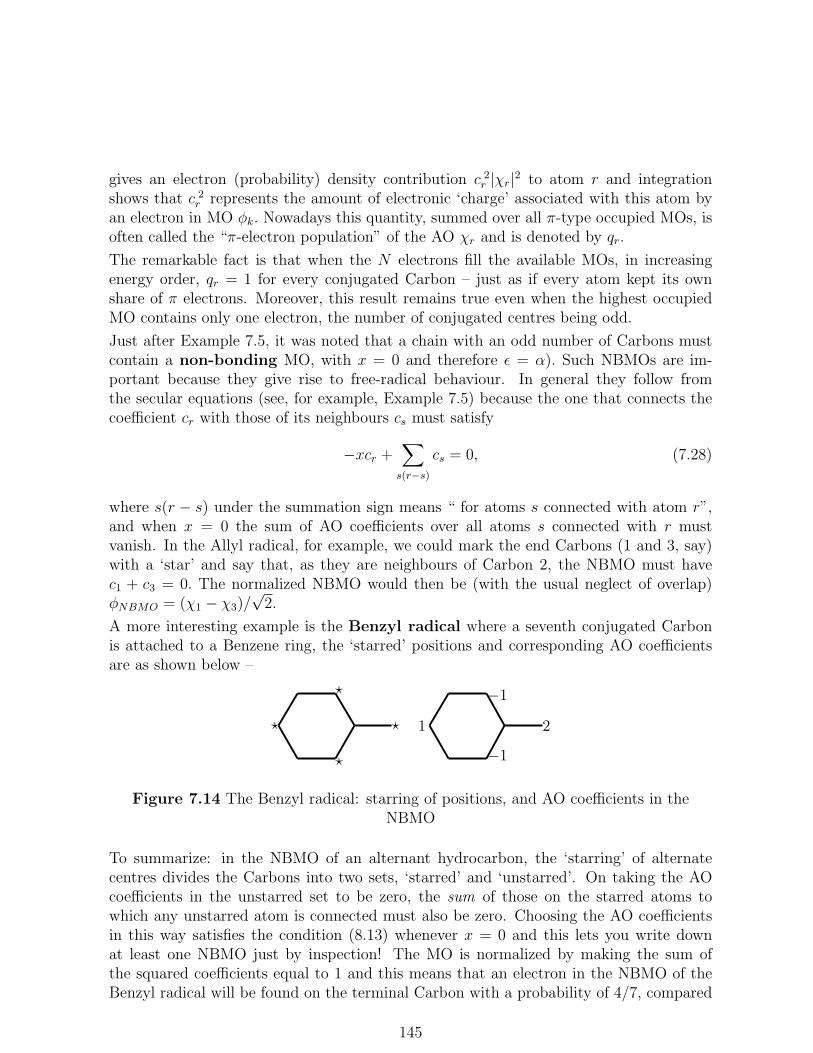
gives an electron (probability) density contribution c 2r |χr|2 to atom r and integration

shows that c 2r represents the amount of electronic ‘charge’ associated with this atom by

an electron in MO φk. Nowadays this quantity, summed over all π-type occupied MOs, isoften called the “π-electron population” of the AO χr and is denoted by qr.

The remarkable fact is that when the N electrons fill the available MOs, in increasingenergy order, qr = 1 for every conjugated Carbon – just as if every atom kept its ownshare of π electrons. Moreover, this result remains true even when the highest occupiedMO contains only one electron, the number of conjugated centres being odd.

Just after Example 7.5, it was noted that a chain with an odd number of Carbons mustcontain a non-bonding MO, with x = 0 and therefore ǫ = α). Such NBMOs are im-portant because they give rise to free-radical behaviour. In general they follow fromthe secular equations (see, for example, Example 7.5) because the one that connects thecoefficient cr with those of its neighbours cs must satisfy

−xcr +∑

s(r−s)

cs = 0, (7.28)

where s(r − s) under the summation sign means “ for atoms s connected with atom r”,and when x = 0 the sum of AO coefficients over all atoms s connected with r mustvanish. In the Allyl radical, for example, we could mark the end Carbons (1 and 3, say)with a ‘star’ and say that, as they are neighbours of Carbon 2, the NBMO must havec1 + c3 = 0. The normalized NBMO would then be (with the usual neglect of overlap)φNBMO = (χ1 − χ3)/

√2.

A more interesting example is the Benzyl radical where a seventh conjugated Carbonis attached to a Benzene ring, the ‘starred’ positions and corresponding AO coefficientsare as shown below –

⋆

⋆

⋆

⋆ 1

−1

−12

Figure 7.14 The Benzyl radical: starring of positions, and AO coefficients in theNBMO

To summarize: in the NBMO of an alternant hydrocarbon, the ‘starring’ of alternatecentres divides the Carbons into two sets, ‘starred’ and ‘unstarred’. On taking the AOcoefficients in the unstarred set to be zero, the sum of those on the starred atoms towhich any unstarred atom is connected must also be zero. Choosing the AO coefficientsin this way satisfies the condition (8.13) whenever x = 0 and this lets you write downat least one NBMO just by inspection! The MO is normalized by making the sum ofthe squared coefficients equal to 1 and this means that an electron in the NBMO of theBenzyl radical will be found on the terminal Carbon with a probability of 4/7, compared

145

with only 1/7 on the other starred centres. The presence of this odd ‘unpaired’ electronaccounts for many of the chemical and physical properties of alternant hydrocarbons withone or more NBMOs. Such electrons easily take part in bonding with other atoms orchemical groups with singly occupied orbitals; and they are also easily ‘seen’ in electronspin resonance (ESR) experiments, where the magnetic moment of the spin couples withan applied magnetic field. The Benzyl radical, with its single loosely bound electron, isalso easily converted into a Benzyl radical anion by accepting another electron, or into acation by loss of the electron in the NBMO. The corresponding ‘starred’ centres then geta net negative or positive charge, which determines the course of further reactions.

To show how easy it is to play with such simple methods you could try to find the NBMOfor the ‘residual molecule’ which results when you take away one CH ‘fragment’ from theNaphthalene molecule shown in Figure 7.14 The system that remains when you choosethe ‘top’ Carbon on the right is

⋆

⋆

⋆⋆

⋆

where the starred positions have been chosen as shown. You should try to attach thenon-zero AO coefficients in the NBMO.

The NBMO is important in the discussion of chemical reactions. The ‘taking away’of the CH group in this example actually happens (we think!) when an NO +

2 groupcomes close to the Carbon: it is ‘thirsty’ for electrons and localizes two π electrons in theCarbon 2p AO, changing the hybridization so that they go into a tetrahedral hybrid andleave only 8 electrons in the 9-centre conjugated system of the residual molecule. TheNO2 group then bonds to the Carbon in this ‘activated complex’, which carries a positivecharge (still lacking 1 electron of the original 10): an electron is then removed from theattached Hydrogen, which finally departs as a bare proton! Just before that final step, theenergy (E ′) of the residual molecule is higher than the energy (E) of the original moleculeand the difference A = E ′−E is called the Activation Energy of the nitration reaction.

Any change you can make in the original molecule (e.g. replacing another Carbon by aNitrogen) that lowers the Activation Energy will make the reaction go more easily; andthat’s the kind of challenge you meet in Chemistry.

(Notice that we’ve been talking always about total π-electron energies, estimated as sumsof orbital energies, and we’re supposing that there are no big changes in the energies ofthe σ bonds. These are approximations that seem to work! – but without them therewould be little hope of applying quantum mechanics in such a difficult field.)

It’s time to move on – this is not a Chemistry book! But before doing so let’s rememberthat nearly all the molecules we’ve been dealing with in this section have been built upfrom only two kinds of atom – Hydrogen, with just one electron, and Carbon, with six.And yet ‘Carbon chemistry’ is so important in our daily life that we can’t do without it:hydrocarbons give us the fuels we need for driving all kinds of machines (in our factories)and vehicles (from scooters to heavy transport); also for heating and cooking; and forpreparing countless other materials (from drugs to plastics and fabrics such as nylon).

146

Remember also that our own bodies are built up almost entirely from elements near thebeginning of the Periodic Table, Carbon and Hydrogen in long chain molecules, along withsmall attached groups containing Nitrogen and Oxygen, and of course the Hydrogen andOxygen in the water molecules (which make up over 50% of body mass). When Calciumand Phosphorus are added to the list (in much smaller quantities) these six elementsaccount for about 99% of body mass!

7.7 Connecting Theory with Experiment

The main ‘bridge’ between so much abstract theory and the things we can measure in thelaboratory, the observables, is provided by a number of electron density functions. InChapter 4 we introduced a ‘density matrix’, in the usual finite-basis representation, whereit was used to define the Coulomb and exchange operators of self-consistent field (SCF)theory. But because we were dealing with closed-shell systems, where the occupiedorbitals occurred in pairs (one with spin factor α and a ‘partner’ with spin factor β) wewere able to ‘get rid of spin’ by integrating over spin variables. Then, in studying theelectronic structure and some of the properties of atoms (in Chapter 5), we took the ideaof density functions a bit further and began to see how useful they could be in dealingwith electronic properties. You should look again at the ideas developed in Examples 5.6and 5.7 and summarized in the ‘box’ (5.33). Finally, in Chapter 6, we were able to extendthe same ideas to molecules; so here you’ll find nothing very new.

It will be enough to remind ourselves of the definitions and fill in some details. The spinlesselectron density function, for a system with an N -electron wave function Ψ(x1,x2, ...xN )is

P (r1) =

∫

ρ(x1)ds1, (7.29)

where ρ(x1) is the density with spin included, as defined in (5.24), and arises from theproduct |ΨΨ∗| on integrating over all variables except x1. Although the variable has beencalled x1 that’s only because we chose the first of the N variables to keep ‘fixed’ inintegrating over all the others: the electrons are indistinguishable and we get the samedensity function whatever choice we make – so from now on we’ll often drop the subscriptin one-electron functions, using just P (r) or ρ(x). The function P (r) is often called, forshort, the “charge density” since it gives us a clear picture of how the total electroniccharge is ‘spread out’ in space.

We’ll continue to use the N -electron Hamiltonian

H =∑

i

h(i) + 12

∑

i 6=j g(i, j), (7.30)

where h(i) and g(i, j) are defined in Chapter 2, through equations (2.2) and (2.3), andthe 1-electron operator h(i) contains a term V (i) for the potential energy of electron i inthe field of the nuclei. The potential energy of the whole system follows in terms of the

147

state function Ψ as

〈Ψ|∑

i

V (i))|Ψ〉 = N

∫

Ψ∗(x1,x2, ...xN )V (1)Ψ(x1,x2, ...xN)dx1dx2 ... dxN

=

∫

V (1)ρ(x1)dx1

=

∫

V (1)P (r1)dr1,

where the first step expresses the expectation value as N times the result for Electron 1;the next step puts it in terms of the density ρ(x1) with spin included; and finally, sinceV (1) is spin-independent, the spin integrations can be done immediately and introducethe ‘spinless’ density P (r1) defined in (7.14)

The spinless density ‘matrix’ is defined similarly:

P (r1; r′1) =

∫

s′1=s1

ρ(x1;x′1)ds1 (7.31)

where ρ(x1;x′1) = N

∫

Ψ(x1,x2, ...xN )Ψ∗(x′

1,x2, ...xN )dx2, ...xN) is the density matrixwith spin included, as defined in (5.26), the prime being used to protect the variable inΨ∗ from the action of any operator. To express the expectation value of an operator sumyou can make similar steps (you should do it!) Thus, for the kinetic energy with operatorT(i) for electron i,

〈Ψ|∑

i

T(i))|Ψ〉 = N

∫

Ψ∗(x1,x2, ...xN )T(1)Ψ(x1,x2, ...xN)dx1dx2 ... dxN

=

∫

x′

1=x1

T(1)ρ(x1;x′1)dx1

=

∫

r′1=r1

T(1)P (r1; r′1)dr1.

Those are one-electron density functions, but in Example 5.7 we found it was possibleto generalize to two- and many-electron densities in a closely similar way. Thus a ‘pair’density (spin included) is defined as

π(x1,x2) = N(N − 1)

∫

Ψ(x1,x2 ...xN)Ψ∗(x1,x2 ...xN )dx3, ...xN

and the density matrix follows on putting primes on the variables x1,x2 in the Ψ∗ fac-tor. With this definition, the expectation value of the electron interaction term in theHamiltonian becomes (remember, the prime on the Σ means “no term with j = i”)

〈Ψ|∑′

(i,j)g(i, j)|Ψ〉 =

∫

[g(1, 2)π(x1,x2;x′1,x

′2)](x′

1=x1,x′

2=x2)dx1dx2.

148

As g(1, 2) is just an inverse-distance electron repulsion, without spin dependence, the spinintegrations can be performed immediately and the primes can be removed. The result isthus

〈Ψ|∑′

(i,j)g(i, j)|Ψ〉 =

∫

[g(1, 2)Π(r1, r2)]dr1dr2.

(The notation is consistent: Greek letters ρ and π are used for the density functions withspin included; corresponding capitals, P and Π for their spin-free counterparts.)

In summary, π(x1,x2) = N(N − 1)∫

Ψ(x1,x2 ...xN )Ψ∗(x1,x2 ...xN)dx3, ...xN and

Π(r1, r2) =

∫

π(x1,x2)ds1ds2 (7.32)

is a 2-electron probability density: it gives the probability of two electrons (any two)being found simultaneously ‘at’ points r1 and r2 in ordinary 3-space, with all the othersanywhere. (Remember this function is a density, so to get the actual probability of findingtwo electrons in tiny volume elements at points r1 and r2 you must multiply it by thevolume factor dr1dr2.)

The function Π(r1, r2) describes the correlation between the motions of two electronsand in IPM approximation turns out to be non-zero only when they have the same spin.This is one of the main challenges to the calculation of accurate many-electron wavefunctions. Fortunately we can go a long way without meeting it!

Some applications

So far we’ve been thinking mainly of an isolated system, which can stay in adefinite energy eigenstate ‘forever’ – such states being stationary. To makethe system change you must do something to it; you must disturb it and asmall disturbance of this kind is called a perturbation. The properties

of the system are measured by the way it reacts to such changes.

Response to an applied electric field

The simplest properties of molecules are the ones that depend directly onthe charge density, described by the function P (r) defined in (7.29). Andthe simplest perturbation you can make is the one due to an electric fieldapplied from outside the molecule. This will change the potential energy ofElectron i in the Hamiltonian H, so that (using x, y, z for the componentsof an electron’s position vector r,

V (i)→ V (i) + δV (i).

When the ‘external’ field is uniform and is in the z-direction, it arisesfrom the electric potential φ as Fz = −∂φ/∂z; and we may thus choose

149

φ = −Fzz, which takes the value zero at the origin of coordinates. Thepotential energy of electron i (of charge −e) due to the applied field is then−eφ = Fzez and represents the change δV (i) in the electron’s potentialenergy. Thus a uniform field in the z-direction will produce a perturbationδV (i) = Fzezi, for every electron i. (Remember, Fz is used for the fieldstrength so as not to mix it up with the energy E).

Supposing Fz to be constant, its effect will be to produce a small polar-ization of the system by urging the electron in the (negative) direction ofthe field (since the electron carries a negative charge −e) and this meansthe probability function will ‘lean’ slightly in the the field direction. Thiseffect will be small: if the change in the wavefunction is neglected in a firstapproximation the change in expectation value of H will be, summing overall electrons,

δE = 〈δH〉 = 〈δV 〉 = Fze

∫

zP (r)dr.

This may be written δE = Fzµz where µzis the z-component of the electricmoment of the electron charge density, which is an experimentally mea-surable quantity. Of course this is a ‘first-order’ result and doesn’t dependon the perturbation of the density function P (r), which is also proportionalto the applied field but is more difficult to calculate. When that is done theresult becomes δE = FzMz+

12F

2z αzz, where αzz is another experimentally

measurable quantity; it is a component of the electric polarizability

tensor but its calculation requires perturbation theory to second order.

Response to displacement of a nucleus

As a second example let’s think of internal changes in the molecule, wherethe change δV in the electronic potential energy function is caused by thedisplacement of a single nucleus. Use X, Y, Z for the coordinates of anucleus (n, say) and think of the displacement in which X → X + δX.The change of interaction energy between electron i and nucleus n will beδV (ri) from electron i. Summing over all electrons gives the total potentialenergy change δV (r) at any point r due to the whole electron distribution;and we again use the result

δE = 〈δH〉 = 〈δV 〉 =∫

δV (r)dr.

150

Now divide both sides by δX and go to the limit where δX → 0, to obtain

Fnx =

∫

Fnx(r)P (r)dr, (7.33)

where you will remember that (by definition)

−(∂E/∂X) = Fnx,

is the total force on nucleus n, and

−(∂Fnx(r)/∂X) = Fnx(r),

is the force due to one electron at point r.

This is the famous Hellmann-Feynman theorem, first derived in Chap-ter 6: in words it says that the forces acting on the nuclei (which opposetheir mutual electrostatic repulsions –and keep the molecule together) canbe calculated by ‘summing’ the attractions due to the amount of chargeP (r)dr in volume element dr over the whole ‘charge cloud’. The interpre-tation is purely ‘classical’: the electron probability density may be treatedas a static distribution of negative charge in which the positive nuclei areembedded. In Chapter 6 we said “This beautiful result seems too good tobe true!” and you should go through the derivation again to understandwhat conditions apply and why you must be cautious in using it. At leastit gives a solid foundation for the ideas contained in Section 6.3, where weintroduced electron populations of orbital and overlap regions in LCAOapproximations to the density function P (r).

There are very many other experimentally observable effects that dependdirectly on the electron density in a molecule (some already studied, like theenergy shifts of inner shell electrons, perturbed from their free-atom valuesby the molecular environment; the response to the approach of chargedchemical groups, such as radical ions and cations; and the whole field ofelectronic spectroscopy, which depends on the time-dependent perturba-tions due to oscillating fields; and so on. But to close this chapter it’sworth trying to fill one gap in the theoretical methodology built up so far:we haven’t said very much about magnetic properties – and yet some ofthe most powerful experimental techniques for getting information about

151

atomic and molecular structure involve the application of strong :mag-netic fields. One thinks in particular of Nuclear Magnetic Resonance

(NMR) and Electron Spin Resonance (ESR), which bring in the spins

of both electrons and nuclei. So we must start by thinking of how a systemresponds to the application of a magnetic field.

Response to an applied magnetic field

Again let’s take the simplest case of a uniform field. Whereas an electricfield – a vector quantity – F with scalar components Fx, Fy, Fz in a Carte-sian system, can be defined as the gradient of a scalar potential functionφ, that is not possible for a magnetic field. If you look at Chapter 4 ofBook 10 you’ll see why: briefly, divB = 0 at every point in free space;but if B were the gradient of some scalar potential φmag that wouldn’t bepossible in general. On the other hand, B could be the curl of some vectorquantity, A, say. (If you’ve forgotten about operators such as grad, divand curl, you’ll need Book 10.)

Now we’re ready to show how the motion of a particle of charge q is modi-fied by the application of a magnetic field. First of all, remember how thekinetic energy T is defined: T = (1/2m)

∑

p 2i , where the index i runs over

components x, y, z and px, for example, is the x-component of momentumpx = mvx = mx – x being short for the time-derivative dx/dt. Also, whenthere is a potential energy V = V (x, y, z) = qφ(x, y, z) the total energy ofthe particle is the Hamiltonian function

E = H(x, y, z, px, py, pz) = T + V,

but the Lagrangian function

L(x, y, z, px, py, pz) = T − V ;

named after the French mathematician Lagrange, is equally important.Either can be used in setting up the same equations of motion, but herewe’ll use Lagrange’s approach.

The Lagrangian for a single particle in a static electric field is thus

L = 12mv

2 − qφ,in terms of the speed v of the particle. In terms of L, the momentumcomponents can be expressed as px = (∂L/∂x) = (∂T/∂x), since φ is

152

velocity-independent. In the presence of a magnetic field, however, weknow there is a transverse force depending on the particle velocity vectorv and the magnetic flux vector B. We want to add a term to L (which is ascalar), depending on charge, velocity and B (or A), which can lead to thecorrect form of this so-called Lorentz force.

The simplest possibility would seem to be the scalar product q(v ·A), whichleads to

L = 12mv

2 + q(v · A)− qφ, (7.34)

and a ‘generalized’ momentum component

px = (∂L/∂x) = mx+ qAx − qφ. (7.35)

This leads to the correct Lorentz force

Fmag = qv × B = qv × curlA

when we calculate the rate of change of particle momentum arising fromthe term q(v · A) in (7.34), as we show in Example 7.10

Example 7.10 Showing that the new equations lead to the correct Lorentzforce.

We want to show that the field-modified equations, (??) and (??) lead tothe Lorentz force Fmag = qv × B. First we write the Newtonian equationsof motion Fx = mx etc. (i.e. Force = mass x acceleration) in Lagrangianform, taking one component at a time. The left-hand side can be written

Fx = −(∂U/∂x) = (∂L/∂x)

(rate of decrease of potential energy U in the x-direction). The right-handside depends only on velocity, through the kinetic energy T = 1

2mx2: thus

∂T/∂x = mx and therefore

Fx = mx =d

dt

(

∂T

∂x

)

=d

dt

(

∂L

∂x

)

,

since the potential energy U does not depend on velocity.

153

The Newtonian equations can thus be replaced by

d

dt

(

∂L

∂x

)

=∂L

∂x

– with similar equations for the y- and z-components.

Example 7.10 Showing that the new equations lead to the correct Lorentzforce.

We want to show that the field-modified equations, (7.34) and (7.35) leadto the Lorentz force Fmag = qv×B. First we write the Newtonian equationsof motion Fx = mx etc. (i.e. Force = mass x acceleration) in Lagrangianform, taking one component at a time. The left-hand side can be written

Fx = −(∂U/∂x) = (∂L/∂x)

(rate of decrease of potential energy U in the x-direction). The right-handside depends only on velocity, through the kinetic energy T = 1

2mx2: thus

∂T/∂x = mx and therefore

Fx = mx =d

dt

(

∂T

∂x

)

=d

dt

(

∂L

∂x

)

,

since the potential energy U does not depend on velocity.

The Newtonian equations can thus be replaced by

d

dt

(

∂L

∂x

)

=∂L

∂x

– with similar equations for the y- and z-components.

Turning now to the generalized momentum vector p, whose x-componentis given in (??), when the applied fields are time-independent its rate ofchange will be

(d/dt)p = (d/dt)mv + q(d/dt)A.

The first term on the right is the usual mass × acceleration of Newton’slaw (the second term being the change resulting from the magnetic field)

154

and refers to the ordinary ‘mechanical’ momentum change. So we writethe equation the other way round, as

mv = p− qA.

The time derivative of p follows from the Lagrangian equations of motion(at the beginning of this Example), namely (for the x-component),

d

dt

(

∂L

∂x

)

=∂L

∂x.

Thus, (∂L/∂x) – which is the generalized momentum x-component – hasa time derivative px and this is equated to (∂L/∂x). When the magneticfield is included it follows that

px = (∂L/∂x) = −q(∂φ/∂x) + qvx∂(Ax/∂x).

The second term in the expression for F = mv is −qA and as we have takenA = 1

2B× r, we can easily calculate its time rate of change. On taking thecomponents one at a time and remembering that the position vector r hascomponents x, y, z. we obtain(

dAx

dt

)

=

(

∂Ax

∂t

)

+

(

∂Ax

∂x

)(

dx

dt

)

+

(

∂Ax

∂y

)(

dy

dt

)

+

(

∂Ax

∂z

)(

dz

dt

)

,

with similar expressions for the y- and z-components. Note that the firstterm on the right will be zero because A has no explicit dependence ontime. The second term in the expression for F = mv is −qA and as wehave taken A = 1

2B× r, we can easily calculate its time rate of change. Ontaking the components one at a time and remembering that the positionvector r has components x, y, z. we obtain(

dAx

dt

)

=

(

∂Ax

∂t

)

+

(

∂Ax

∂x

)(

dx

dt

)

+

(

∂Ax

∂y

)(

dy

dt

)

+

(

∂Ax

∂z

)(

dz

dt

)

,

with similar expressions for the y- and z-components. Note that the firstterm on the right will be zero because A has no explicit dependence ontime. The second term in the expression for F = mv is −qA and as wehave taken A = 1

2B× r, we can easily calculate its time rate of change. On

155

taking the components one at a time and remembering that the positionvector r has components x, y, z. we obtain(

dAx

dt

)

=

(

∂Ax

∂t

)

+

(

∂Ax

∂x

)(

dx

dt

)

+

(

∂Ax

∂y

)(

dy

dt

)

+

(

∂Ax

∂z

)(

dz

dt

)

,

with similar expressions for the y- and z-components. Note that the firstterm on the right will be zero because A has no explicit dependence ontime.

On substituting both terms into the force equation F = mv = p − qA thex-component follows as

Fx = −q∂φ

∂x+ q

[(

∂Ay

∂x− ∂Ax

∂y

)

y −(

∂Ax

∂z− ∂Az

∂x

)

z

]

.

The two terms in round brackets can be recognised as, respectively, the z-and y-components of the vector curlA; and when the coefficients y and zare attached the result in square brackets is seen to be the x-component ofthe vector product v × curlA.

Finally, then, in vector notation F = qE+ q(v× B) where the electric fieldvector is here denoted by E, while the other term Fmag = q(v × curlA) isthe Lorentz force.

Molecules in magnetic fields

In Section 6 of Chapter 5 we noted that whenever a system containedunpaired electrons there would be a tiny interaction between the electron

spin, with its resultant magnetic dipole, and any external magnetic field.A free spin interacts with a magnetic field B through a ‘coupling term’gβB · S, where the ‘g-value’ is very close to 2 and β = e~/2m (the “Bohrmagneton”). So there will be a small perturbation of the many-electronHamiltonian of the form

H′Z = gβ∑

i

B · S(i), (7.36)

the summation being over all electrons. This is the spin-field “Zeemaninteraction”.

There will also be an interaction between the spin dipole and the magneticfield produced by motion of the electrons, which will depend on the veloc-ity with which they are moving. In the case of an atom, the spatial motion

156

around the nucleus was represented by an angular momentum operator,giving rise to spin-orbit coupling through a perturbation

H′mag = β∑

i

B · L(i). (7.37)

By taking account of these two perturbations we were able to predict thefine structure of atomic energy levels, which could be ‘seen’ experimen-tally in electronic spectroscopy.

In the case of a molecule things are a bit more difficult: there will be severalnuclei instead of one, so an electron is not in a spherically symmetrical fieldand will not be in a state of definite angular momentum – which is said to be‘quenched’ by the presence of other nuclei. That means the velocity of theelectron will be variable and spread out through space, corresponding to a‘current’ of probability density; and in defining this we must take accountof the magnetic field. We also need to generalize the spin density, definedas the excess of up-spin electron density, Pα(r), over down-spin, Pα(r) (see(5.32). We can, however, do both things at the same time by going backto first principles.

Property Densities

Suppose we are interested in some observable quantity, call it X, withassociated operator X(i) for electron i. The expectation value of X, for thewhole N -electron system will be

〈Ψ|X|Ψ〉 =

∫

Ψ∗(x1,x2, ...xN)XΨ(x1,x2, ...xN)dx1dx2 ... dxN

= N

∫

Ψ∗(x1,x2, ...xN)X(1)Ψ(x1,x2, ...xN)dx1dx2 ... dxN .

– since every electron gives the same contribution as ‘Electron 1’. Bymoving the Ψ∗ factor to the right and changing variable x1 to x′1 (so theoperator will not touch it), we can rewrite this result as

〈Ψ|X|Ψ〉 =∫

[X(1)ρ(x1;x′1)]x′

1=x1dx1,

where ρ(x1;x′1) is the 1-electron density matrix and the two variables

are identified after the operation with X(1).

157

The whole integrand in the last equation is an ordinary density functionand, when integrated over all space, gives the expectation value of X forthe whole system. We’ll call it a property density for X and denote itby

ρX(x) = [Xρ(x;x′)]x′=x, (7.38)

where the subscripts on the variables in the one-electron density matrix,no longer necessary, are dropped from now on.

Spinless Properties

You’ve already dealt with similar density functions, usually for propertiesthat are spin-independent. In that case you can integrate over spin vari-ables immediately in getting the expectation value and obtain, instead of(7.38), a spinless density function

PX(r) = [XP (r; r′)]r′=r. (7.39)

If you write V instead of X, for potential energy of the electrons in thefield of the nuclei, and identify the variables straight away (V ) being just afunction of position in ordinary space), then all should be clear: the densityof potential energy becomes

PV (r) = V (r)P (r),

since V is just the multiplier V (r). The density is thus the amount ofpotential energy per unit volume for an electron at point r and integrationover all space gives the expectation value of the potential energy of thewhole electron distribution.

Spin Density

Now let’s think of the density of a component of spin angular momen-

tum (if the electron is ‘smeared out’ in space, with probability densityP (r) per unit volume, then so is the spin it carries!). On taking X = Sz,and using (7.38) we get

ρSz(x) = [Sz ρ(x;x′)]x′=x.

For any kind of wave function ρ(x;x′) will have the form (Read Example5.6 again, and what follows it, then think about it!)

ρ(x;x′) = Pα(r; r′)α(s)α(s′) + Pβ(r; r

′)β(s)β(s′).

158

The spin operator in (7.40) will multiply α(s) by 12 , but β(s) by −1

2 andthen, removing any remaining primes, (7.40) will become (check it out!)

ρSz(r) =12 [Pα(r)− Pβ(r)]. (7.40)

This result, as you would expect, is simply (in words)

“Density of up-spin electrons minus density of down-spin, times magnitudeof spin angular momentum”.

Since ρ has usually been reserved for functions of the space-spin variablex, the result is often written instead as

Qz(r) =12 [Pα(r)− Pβ(r)]. (7.41)

Similar densities, Qx, Qy, may also be defined, but in practice the applied magnetic field (e.g. in NMR

and ESR experiments) is usually chosen to fix the ‘z-direction’.

Densities that depend on motion of the electrons

The other density functions needed refer to electronicmotion, for generalityin the presence of a magnetic field: they are a density of kinetic energy(which is a scalar quantity) and a current density (a vector density arisingfrom the linear momentum).

Kinetic Energy Density

In (7.34) we proposed the kinetic energy operator T = 12mv2−e(v·A) for an

electron moving in a magnetic field B, arising from a vector potential A;and in this case we also derived a ‘generalized’ momentum operator(7.35),namely p = mr − eA, whose first term is just the Newtonian quantity mv

– usually denoted by p when there is no magnetic field. To avoid confusionit’s convenient to give the generalized momentum vector a new symbol,writing it as

π = mr − eA (7.42)

and calling it, by its usual name, the “gauge invariant momentum”.

When there is no magnetic field, the 1-electron KE term in the Hamiltoniancan be written T = (1/2m)p2 and it would seem that a kinetic energydensity could be defined (cf. (7.39)) as

PT0(r) = (1/2m)[p2 P (r; r′)]r′=r,

where subscript zero indicates zero magnetic field.

159

Unfortunately this definition is not completely satisfactory because it leadsto a quantity with both real and imaginary parts, whereas the kinetic en-ergy contributions must be both real and positive at all points in space.One way out of this difficulty is simply to take the real part of the lastexpression as a more satisfactory definition; another is to replace the oper-ator p2 by p · p†, where the adjoint operator p† (obtained by changing thesign of i) works on the variables in the wave function Ψ∗. In the secondcase the KE density becomes

PT0(r) = (1/2m)[p · p† P (r; r′)]r′=r. (7.43)

(This is still not absolutely satisfactory if one wants to know how muchKE comes from a finite part of space, when integrating to get the totalexpectation value, for it contains terms depending on the surface boundingthe chosen region. But for all normal purposes, which involve integrationover all space, it may be used.)

In the presence of a magnetic field the operator p is replaced by the ‘gen-eralized’ momentum operator π, defined in (7.42), and the natural gener-alization of the KE density is

PT(r) = (1/2m)[π · π† P (r; r′)]r′=r. (7.44)

Like the field-free result, this definition is normally satisfactory.

Probability current density

Whenever the probability distribution, described by the 1-electron densityP (r), is changing in time we need to know how it is changing. There willbe a flow of density out of (or into) any volume element dr and it mustbe described in terms of a velocity component vα (α = x, y, z) in ordinaryspace. (Think of the wave packet discussed in Section ? of Book 11.)

Here we’ll look for a current density function with components Jα(r) suchthat

Pvα(r) = (1/m)[pα P (r; r′)]r′=r,

which we know will lead, on integrating over all space, to the expectationvalue 〈vα〉 of electronic velocity along the α direction. Again this gives ingeneral an unwanted imaginary component, which may be dropped; and

160

when the magnetic field is admitted the most satisfactory definition is

Pvα(r) = m−1Re[πα P (r, r′)]r′=r. (7.45)

This gives a current density which is everywhere real and positive and givesthe correct expectation value on integrating over all space.

Finite basis approximations

Of course, if we want to actually calculate a molecular electronic propertywe have to use an approximation in which the orbitals used (e.g. the MOs)are expressed as linear combinations of basis functions (e.g. AOs centredon the various nuclei). This finite basis approximation was first introducedin Chapter 4 (Section 4.4) and allows us to convert all equations intomatrix

equations. For example any MO

φK = cK1χ1 + cK2χ2 + ... + cKrχr + ... + cKmχm

can be expressed in matrix form, as the row-column product

φK = (χ1 χ2 ... χm)

cK1

cK2

..

..

cKm

= χcK , (7.46)

where cK stands for the whole column of expansion coefficients and χ forthe row of basis functions. So the X operator will be represented in the χ-basis by the matrix X, with elements Xrs = 〈χr|X|χs〉, and its expectationvalue for an electron in φK will be

〈φK |X|φK〉 =∑

r,s

c∗Kr〈χr|X|χs〉cKs

=∑

r,s

c∗KrXrscKs

= cK†XcK (7.47)

– so, you see, an operator (set in the special typeface as X) is representedby a corresponding matrix X (set in boldface), while a function, such asφK , is represented by a single-column matrix cK containing its expansion

161

coefficients; and the complex conjugate of a function is indicated by addinga ‘dagger’ to the symbol for its column of coefficients. Once you get usedto the notation you can see at a glance what every equation means. Asa simple illustration of how things work out in a finite basis we can usea very rough approximation to estimate the velocity expectation value foran electron moving along a 1-dimensional chain of Carbon atoms.

Example 7.11 Calculation of a ring currentIn Example 7.9 we joined the ends of a chain of N Carbon atoms to make a ring, considering onlythe π electrons (one from each atom) and using Huckel approximations to calculate the MOs φk andcorresponding energy levels ǫk. In the absence of an applied magnetic field, the electron velocity operatoris v = (1/m)p and we’ll choose the momentum operator for a component p in the ‘positive’ direction (i.e.from Atom n to Atom n+ 1 as you go along the chain.)

Suppose we want the expectation value 〈v〉 for motion in this direction and for any allowed value of k.Since any velocity operator v = (1/m)p contains a factor (~/i), and is thus pure imaginary, its expectationvalue in any state with a real wave function must be zero. But Example 7.9 showed that, for a ring of Natoms, complex eigenfunctions of the form

φk = Ak

∑

n

χn exp(2πink/N) (Ak = 1/√N)

could be found. The MO of lowest energy is φ0 = A0(χ1+χ2+ ...+χ6) and, being real, will have zero valueof the velocity expectation value. But the MOs with k = ±1 form a degenerate pair, whose wave functions

are complex conjugate. The expectation value in state φk will be 〈φk|v|φk〉 =∑

n,n′ c(k)∗n 〈χn|v|χn′〉c(k)n′

and tdo evaluate this quantity, which measures the expected electron probability current, we need only

the matrix elements 〈χn|v|χn′〉 and the AO coefficients c(k)n (given above for any chosen k). If we were

doing an energy calculation, with Huckel approximations, we’d have the 1-electron Hamiltonian h in placeof v; and the n-n′ matrix element would be given an empirically chosen value βnn′ for nearest neighbouratoms, zero otherwise. But here the nearest neighbours of Atom n would have n′ = n + 1 (for positivedirection along the chain) and n′ = n− 1 (for negative direction); and, as the operator v ‘points’ in thedirection of increasing n, the n→ n+ 1 matrix element would have a substantial (but imaginary) value(iγ, say). With this choice, the most suitable approximations would seem to be 〈χn|v|χn+1〉 = iγ and〈χn|v|χn−1〉 = −iγ, other matrix elements being considered negligible.

On using this very crude model, the expectation value of the velocity component for an electron in MOφk, for an N -atom chain, would be

〈φk|v|φk〉 = |Ak|2n=N∑

n=1

[exp(−2πink/N)(iγ) exp(2πi(n+ 1)k/N)

+ exp(−2πink/N)(−iγ) exp(2πi(n− 1)k/N)].

This reduces to (Check it out!– noting that the summation contains N terms)

〈φk|v|φk〉 = −2γ sin(2πk/N).

The example confirms that, even without using a computer (or even a simple calculator!),it’s often possible to obtain a good understanding of what goes on in a complicated many-electron system. Here we’ve found how an IPM approach with the simplest possible

162

approximations can reveal factors that govern the flow of charge density along a carbonchain: a parameter γ (which depends on overlap of adjacent AOs) should be large and theflow will be faster in quantum states with higher values of a quantum number k. Pairs ofstates with equal but opposite values of k correspond to opposite directions of circulationround the ring; and the circulating current produces a magnetic dipole, normal to theplane of the ring. In cyclic hydrocarbons such effects are experimentally observable; andwhen the angular momentum operator p is replaced by the ‘gauge invariant’ operatorπ (which contains the vector potential of an applied magnetic field) it is possible tocalculate a resultant induced magnetic dipole – again experimentally observable. Infact, the quantum number k in a ring current calculation is the analogue of an angular

momentum quantum number in an atomic calculation. Chapter 7 has set out most ofthe mathematical tools necessary for an ‘in depth’ study of molecular electronic structureand properties – even if only at IPM level. But, for now, that’s enough!

In Chapter 8, we’ll start looking at more extended systems where there may be manythousands of atoms. Incredibly, we’ll find it is still possible to make enormous progress.

163

Chapter 8

Some extended structures in 1-,2-

and 3-dimensions

8.1 Symmetry properties of extended structures

In earlier chapters of this book we’ve often talked about “symmetry properties” of asystem; these have been, for example, the exchange of two or more identical particles, ora geometrical operation such as a rotation which sends every particle into a new position.Such operations may form a symmetry group when they satisfy certain conditions.We have met Permutation Groups in introducing the Pauli Principle (Section 2.4 ofChapter 2); and Point Groups, which contain geometrical operations that leave onepoint in the system unmoved, in studying molecules (e.g. in Example 7.5 of this book).But when we move on to the study of extended structures such as crystals, in whichcertain structural ‘units’ may be repeated indefinitely (over and over again) as we gothrough the crystal, we must admit new symmetry operations – called translations. Sothis is a good point at which to review the old and start on the new.

The Point Groups

Here we’ll use one or two simple examples to introduce general ideas andmethods, without giving long derivations and proofs. As a first examplelet’s look at the set of operations which, when applied to a square plate(or ‘lamina’), leave it looking exactly as it did before the operation: theseare the operations which “bring it into self-coincidence”. They are namedas shown in the following Figure 8.1, where those labelled with a C are allrotations around a vertical axis through the centre of the square, whilethose with a σ refer to reflections across a plane perpendicular to it(the arrow heads indicate a direction of rotation, while the double-headedarrows show what happens in a reflection). Thus, rotation C4 sends the

164

square corners labelled 1, 2, 3, 4 into 2, 3, 4, 1 and similarly σ1 interchangescorners 2 and 4, leaving 1 and 3 where they were.

1

2

3

4

C2C4

C4

σ2σ′2

σ1

σ′1

Figure 8.1 Symmetry operations: square lamina (see text)

Note that subscripts 1 and 2 on the reflection operations label differentreflection planes and, when that is not enough, a prime has been addedto the σ to show a different type of reflection (e.g. one which interchangesopposite sides of the square instead of opposite corners). The rotations Cnstand for those in the positive sense (anti- clockwise), through an angle2π/n, while Cn stands for a similar operation, but in the negative sense(i.e. clockwise). In this example the operations do not include “turningthe plate over”, because the top and bottom faces may look different; if theylooked exactly the same we’d have to include another symmetry operationfor the interchange.

Note also that symmetry operations aren’t always ones you can actuallydo! A reflection, for example, is easy to imagine – sending every pointon the lamina into its ‘mirror image’ on the other side of the reflectionplane – but could only be done by breaking the lamina into tiny pieces andre-assembling them!

The various operations, defined and named in Figure 8.1, can be collectedand set out in a Table –as below:

165

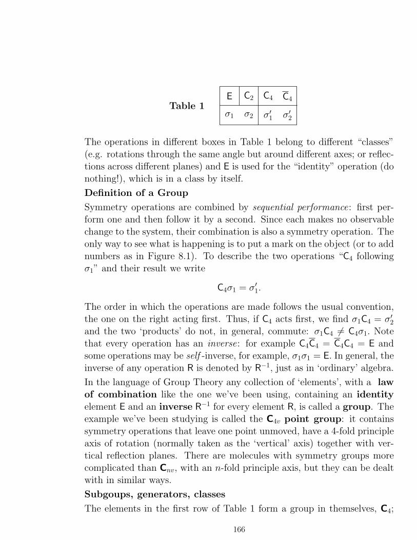
Table 1E C2 C4 C4

σ1 σ2 σ′1 σ′2

The operations in different boxes in Table 1 belong to different “classes”(e.g. rotations through the same angle but around different axes; or reflec-tions across different planes) and E is used for the “identity” operation (donothing!), which is in a class by itself.

Definition of a Group

Symmetry operations are combined by sequential performance: first per-form one and then follow it by a second. Since each makes no observablechange to the system, their combination is also a symmetry operation. Theonly way to see what is happening is to put a mark on the object (or to addnumbers as in Figure 8.1). To describe the two operations “C4 followingσ1” and their result we write

C4σ1 = σ′1.

The order in which the operations are made follows the usual convention,the one on the right acting first. Thus, if C4 acts first, we find σ1C4 = σ′2and the two ‘products’ do not, in general, commute: σ1C4 6= C4σ1. Notethat every operation has an inverse: for example C4C4 = C4C4 = E andsome operations may be self -inverse, for example, σ1σ1 = E. In general, theinverse of any operation R is denoted by R−1, just as in ‘ordinary’ algebra.

In the language of Group Theory any collection of ‘elements’, with a law

of combination like the one we’ve been using, containing an identity

element E and an inverse R−1 for every element R, is called a group. Theexample we’ve been studying is called the C4v point group: it containssymmetry operations that leave one point unmoved, have a 4-fold principleaxis of rotation (normally taken as the ‘vertical’ axis) together with ver-tical reflection planes. There are molecules with symmetry groups morecomplicated than Cnv, with an n-fold principle axis, but they can be dealtwith in similar ways.

Subgoups, generators, classes

The elements in the first row of Table 1 form a group in themselves, C4;

166

we say C4 is a subgroup of C4v.

All the elements in C4 can be expressed in terms of one element C4: thusC2 = C4C4(= C 2

4 ), C4 = C 34 , E = C 4

4 . We say C4 is a generator of C4.

If we take the elements in the first row of Table 1 and follow them (i.e.multiply from the left), in turn, with σ1 we generate the elements in thesecond row. Thus, the whole group C4v can be generated from only twoelements, C4 and σ1. Often we need to work with only the generators of agroup, since their properties determine the group completely.

The classes within a group each contain symmetry operations which aresimilar except that the axis, or reflection plane, to which they refer hasitself been acted on by a symmetry operation. Thus, the reflection planefor σ2 differs from that for σ1 by a C4 rotation; so σ1 and σ2 are in thesame class – but this class does not include σ′1 or σ

′2.

Space Groups and Crystal Lattices

So far we’ve been looking only at Point Groups, where one point staysfixed in all symmetry operations. But in extended structures like crystalswe must admit also the translation operations in which all points areshifted in the same direction and by the same amount. In symbols, atranslation t sends the point with position vector r into an ‘image’ withr′ = r + t. Moreover, translations and point group operations (which we’lldenote generally by R) can be combined. Thus, a rotation followed by atranslation will send a point at r into an image at r′ = Rr+ t. It is usual todenote this composite operation by (R|t) (not to be confused with a scalarproduct in quantum mechanics!), writing in symbols

r′ = (R|t)r = Rr + t. (8.1)

It is then easily shown (do it!) that the law of combination for such oper-ations is

(R|t)(S|t′) = (RS|t+ Rt′) (8.2)

and that the set of all such operations then forms a Space Group.

In the following example we show how just two primitive translations,call them a1 and a2, can be used to generate a Crystal Lattice in twodimensions. On adding a third primitive translation a3 it is just as easy togenerate a lattice for a real three-dimensional crystal.

167

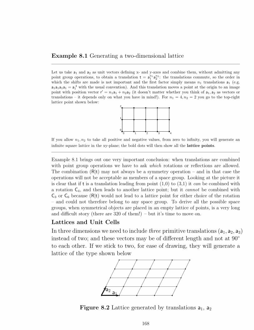
Example 8.1 Generating a two-dimensional lattice

Let us take a1 and a2 as unit vectors defining x- and y-axes and combine them, without admitting anypoint group operations, to obtain a translation t = an1

1 an2

2 : the translations commute, so the order inwhich the shifts are made is not important and the first factor simply means n1 translations a1 (e.g.a1a1a1a1 = a 4

1 with the usual convention). And this translation moves a point at the origin to an imagepoint with position vector r′ = n1a1 + n2a2 (it doesn’t matter whether you think of a1, a2 as vectors ortranslations – it depends only on what you have in mind!). For n1 = 4, n2 = 2 you go to the top-rightlattice point shown below:

0 1 2 3 40

1

2

If you allow n1, n2 to take all positive and negative values, from zero to infinity, you will generate an

infinite square lattice in the xy-plane; the bold dots will then show all the lattice points.

Example 8.1 brings out one very important conclusion: when translations are combinedwith point group operations we have to ask which rotations or reflections are allowed.The combination (R|t) may not always be a symmetry operation – and in that case theoperations will not be acceptable as members of a space group. Looking at the picture itis clear that if t is a translation leading from point (1,0) to (3,1) it can be combined witha rotation C4, and then leads to another lattice point; but it cannot be combined withC3 or C6 because (R|t) would not lead to a lattice point for either choice of the rotation– and could not therefore belong to any space group. To derive all the possible spacegroups, when symmetrical objects are placed in an empty lattice of points, is a very longand difficult story (there are 320 of them!) – but it’s time to move on.

Lattices and Unit Cells

In three dimensions we need to include three primitive translations (a1, a2, a3)instead of two; and these vectors may be of different length and not at 90◦

to each other. If we stick to two, for ease of drawing, they will generate alattice of the type shown below

a1a2

Figure 8.2 Lattice generated by translations a1, a2

168

A general lattice point will then have the position vector (in 3 dimensions)

r = n1a1 + n2a2 + n3a3, (8.3)

where n1, n2, n3 are integers (positive, negative, or zero). The scalar prod-uct that gives the square of the length of the vector (i.e. of the distancefrom the origin to the lattice point) is then

r · r = n 21 (a1 · a1) + n 2

2 (a2 · a2) + n 23 (a3 · a3)

+n1n2(a1 · a2) + n1n3(a1 · a3) + n2n3(a2 · a3)=∑

i

n 2i Sii +

∑

i<j

ninjSij (Sij = ai · aj), (8.4)

where the Sij are elements of the usual metric matrix S and i, j go from1 to 3. When the vectors for the primitive translations are orthogonal andof equal length S is a multiple of the 3 × 3 unit matrix and the transla-tions generate a simple cubic lattice, in which (distance)2 has the usual(Cartesian) form as a sum of squares of the vector components.

Using (8.3), with the oblique axes shown in Figure 8.2, the scalar productdoes not have that simple form; but we can get it back by setting up anew basis of ‘reciprocal vectors’ (not a good name), denoted by b1, b2,

in which a general vector v is expressed as v = v1b1 + v2b2 – and choosingb1 orthogonal to a2, but with length reciprocal to that of a1, and similarlyfor b2. This makes a1 · b1 = a2 · b2 = 1, but a1 · b2 = 0 and a scalar product(r1a1 + r2a2) · (v1b1 + v2b2) will then take the usual form

r · v = r1v1(a1 · b1) + r2v2(a2 · b2) + r1v2(a1 · b2) + r2v1(a2 · b1) = r1v1 + r2v2,

just as it would be for two general vectors in a (Cartesian) 2-dimensionalspace.

The same construction can be made in 3-space, with the primitive trans-lations described by the vectors a1, a2, a3; and with basis vectors b1, b2, b3defining the reciprocal space. But in this case the relationship betweenthe two bases is not so direct: the b vectors must be defined as

b1 =a2 × a3

[a1 a2 a3],

169

with permutations 123→ 231→ 312 giving b2, b3. Here [a1 a2 a3] = a1 ·a2×a3 is the vector triple product which gives the volume of a single unit cell

of the lattice (If you turn back to Section 6.4 of Book 2, you’ll see you didthis long ago!)

Many metals have a crystal structure with a single atom at every latticepoint and in a “free-electron model” we can think of the most loosely boundelectrons as moving freely around the positively charged atomic ‘cores’ fromwhich they came.

Example 8.2 Simple model of a crystal

Let us consider a ‘fundamental volume’ containing a large number G3 of unit cells, G in each of thethree directions a1, a2 and a3. You can think of this as defining a small crystal of the same shape as theunit cell.

First we’ll forget about the atom cores and think of completely free electrons moving in a box providedby the ‘empty lattice’. We know that the energy eigenstates of a free electron are given by φ(r) =M exp(ir · p/~) where r and p represent its position and momentum vectors (as sets of components),while ~ = h/2π is Planck’s constant and M is just a normalizing factor.

When we write position and momentum in the form r1a1+ r2a2+ r3a3 and p1b1+ p2b2+ p3b3, the scalarproduct r · p keeps its Cartesian form and the free-electron wave function becomes

φ(r) = N exp(ir1p1/~) exp(ir2p2/~) exp(ir3p3/~).

Now on changing r1a1 to (r1 +G)a1 we move from the origin to a point G lattice cells further on in thea1 direction; and we want to impose the periodic boundary condition that the corresponding factorin the wave function is unchanged. This means that exp(iGp1/~) must be unity and this requires thatthe argument Gp1/~ must be a multiple of 2π. The same argument applies in the other directions, so wemust insist that

Gp1/~ = κ1(2π), Gp2/~ = κ2(2π), Gp3/~ = κ3(2π),

where κ1, κ2, κ3 are arbitrary (but very large) integers. In other words the only allowed momentumvectors are p = ~k, with components p1 = (2π/G)κ1 etc. – and the vectors are thus

p = (~κ1/G)2πb1 + (~κ2/G)2πb1 + (~κ3/G)2πb3.

It is usual to write the results of Example 8.2 in the form p = ~k where

k = k1(2πb1) + k2(2πb2) + k3(2πb3), (8.5)

Here k is called a vector of k-space and the basis vectors are now taken as 2πb1, 2πb2, 2πb3.

The corresponding 1-electron wave function will then be (adding a normalising factor M)

φ(r) =M exp(ir · p/~) =M exp(ik · r), (8.6)

170

with quantized values of the k-vector components. (Remember that vector components,being sets of numbers, have usually been denoted by bold letters r, while the abstractvectors they represent are shown in ‘sans serif’ type as r) The energy of the 1-electronstate (8.6) can still be written in the free-electron form ǫk = (~2/2m)|k|2, but when theaxes are oblique this does not become a simple sum-of-squares (you have to do sometrigonometry to find the squared length of the k-vector!) .

Of course an empty box, even with suitable boundary conditions, is not a good modelfor any real crystal; but it gives a good start by showing that the ‘fundamental volume’containing G3 lattice cells allows us to set up that number of quantized 1-electron states,represented by points in a certain central zone of k-space. Each state can hold twoelectrons, of opposite spin, and on adding the electrons we can set up an IPM descriptionof the whole electronic structure of the crystal.

8.2 Crystal orbitals

In the ‘empty-lattice’ approximation, we have used free-electron wave functions of the form(8.6) to describe an electron moving with definite momentum vector p = ~k, quantizedaccording to the size and shape of the fundamental volume.

Now we want to recognize the fact that in reality there is an internal structure due to thepresence of atomic nuclei, repeated within every unit cell of the crystal. We’re going tofind that the 1-electron functions are now replaced by crystal orbitals of very similarform

φ(r) =M exp(ik · r)fk(r), (8.7)

where fk(r) is a function with the periodicity of the lattice – having the same value atequivalent points in all the unit cells. This result was first established by the Germanphysicist Bloch and the functions are also known as Bloch functions.

To obtain (8.7) most easily we start from the periodicity of the potential function V (r):if we look at the point with position vector r + R, where R is the displacement

R = m1a1 +m2a2 +m3a3

and m1,m2,m3 are integers, the potential must have the same value as at point r. Andlet’s define an operator TR such that TRφ(r) = φ(r+R). Applied to the potential functionV (r) it produces TRV (r) = V (r+R), but this must have exactly the same value V (r) asbefore the shift: the potential function is invariant against any displacement with integralm’s. The same is true for the kinetic energy operator T and for the sum h = T+V, whichis the 1-electron Hamiltonian in IPM approximation. Thus

TR(hφ) = hTRφ,

h being unchanged in the shift; and in other words the operators h and TR must commute.

171

If we use T1,T2,T3 to denote the operators that give shifts r→ r+a1, r→ r+a2, r→ r+a3(for the primitive translations) then we have four commuting operators (h,T1,T2,T3) andshould be able to find simultaneous eigenfunctions φ, such that

hφ = ǫφ, T1φ = λ1φ, T2φ = λ2φ, T3φ = λ3φ. (8.8)

Now let’s apply T1 G times to φ(r), this being the number of unit cells in each directionin the fundamental volume, obtaining (T1)

Gφ = λ G1 φ. If we put λ1 = eiθ1 this means that

Gθ1 must be an integral multiple of 2π, so we can write θ1 = (κ1/G)× (2π), where κ1 isa positive or negative integer or zero. This is true also for λ2 and λ3; and it follows thatin a general lattice displacement, R = m1a1 +m2a2 +m3a3,

φ(r+R) = TRφ(r) = Tm1

1 Tm2

2 Tm3

3 φ(r).

On introducing the k-vector defined in (8.6), this result becomes

φ(r+R) = TRφ(r) = exp(ik ·R)φ(r). (8.9)

To show that a function φ(r) with this property can be written in the form (8.2) it isenough to apply the last result to the function eik·rf(r), where f(r) is arbitrary: thus

eik·Reik·rf(r+R) = eik·Reik·rf(r).

In other words we must have f(r +R) = f(r) and in that case the most general crystalorbital will have the form

φk(r) = eik·rfk(r) (fk(r) a periodic function) (8.10)

Here the subscript k has been added because the components of the k-vector are essentiallyquantum numbers labelling the states. There is thus a one-to-one correspondence betweenBloch functions and free-electron wave functions, though the energy no longer depends ina simple way on the components k of the k-vector The simplest approximation to a crystalorbital is a linear combination of AOs on the atomic centres: thus, for a 1-dimensionalarray of lattice cells, with one AO in each, this has the general form

φ =∑

n

cnχn, (8.11)

where the χs are AOs on the numbered centres. We imagine the whole 1-dimensionalcrystal is built up by repeating the fundamental volume of G unit cells in both directions,periodicity requiring that cn+G = cn.

In the following example we assume zero overlap of AOs on different centres and use anearest-neighbour approximation for matrix elements of the 1-electron Hamiltonian h.Thus, introducing the so-called coulomb and resonance integrals

〈χn|h|χn〉 = α, 〈χn|h|χn+1〉 = β (8.12)

172

Example 8.3 Crystal orbital for a 1-dimensional chain

With the approximations (8.12), the usual secular equations to determine the expansion coefficients in(8.11) then become (check it out!)

cn−1β + (cn − ǫ)α+ cn+1β = 0 (all n)

and are easily solved by supposing cn = einθ and substituting. On taking out a common factor thecondition becomes, remembering that eiθ + e−iθ = 2 cos θ, (α − ǫ) + 2β cos θ = 0, which fixes ǫ in termsof θ.

To determine θ itself we use the periodicity condition cn+G = cn, which gives eiGθ = 1. Thus Gθ must bean integral multiple of 2π and we can put θ = 2πκ/G, where κ is a positive or negative integer or zero.Finally, the allowed energy levels and AO coefficients in (8.11) can be labelled by κ:

ǫκ = α+ 2β cos(2πκ/G), c κn = exp(2πiκn/G).

The energy levels for a 1-dimensional chain of atoms, in LCAO approximation, shouldtherefore form an energy band of width 4β, where β is the interaction integral 〈χn|h|χn+1〉between neighbouring atoms. Figure 8.4, below, indicates these results for a chain of Hy-drogen atoms, where every χ is taken to be a 1s orbital.

ǫ 4β

(a) (b)

Figure 8.4 Energy Band and part of Crystal Orbital(schematic, see text)

The energy levels are equally spaced around ǫ for a free atom, G ‘bonding’ levels below andG ‘anti-bonding’ levels above. When the number of atoms in the fundamental volume isvery large the levels become so close that they form an almost continuous band, indicatedby the shaded area in (a). The crystal orbitals, being linear combinations of the AOs,have a wave-like form with a wavelength depending on the energy, as indicated in (b).If the nuclear charges were reduced to zero, the AOs would become broader and broaderand the ‘spiky’ crystal orbital would go over into the plane wave for an empty lattice.

8.3 Polymers and plastics

It’s time to look at some real systems and there’s no shortage of them: even plasticbags are made up from long chains of atoms, mainly of Carbon and Hydrogen atoms, all

173

tangled together; and so are the DNA molecules that carry the ‘instructions’ for buildinga human being from one generation to the next! All are examples of polymers.

In Example 8.3 we found crystal orbitals for the π-electrons of a carbon chain, using anearest-neighbour approximation and taking the chain to be straight. In reality, however,carbon chains are never straight, and the C–C sigma bonds are best described in terms ofhybrid AOs, inclined at 120◦ to each other. Polyene chains are therefore usually ‘zig-zag’in form, even when the Carbon atoms lie in the same plane – as in the case shown below:

H

H

H

H

H

H

H

H

H

H

H

Figure 8.5 Picture showing part of a long polyene chain

In the figure, the black dots in the chain indicate the Carbon atoms of the ‘backbone’, towhich the Hydrogens are attached. The molecule is (ideally) flat and each Carbon providesone electron in a π-type AO, which can be visualized as sticking up perpendicular to theplane of the paper. The system is a ‘one-dimensional crystal’ in which each unit cellcontains four atoms, two Carbons and two Hydrogens. As C2H2 is the chemical formulafor Acetylene (which you met in Example 7.3), a polyene of this kind is commonly called‘polyacetylene’ (“many-acetylenes”.)

In Example 8.3, we used a simplified model in which (i) the zig-zag chain was replaced bya straight chain; (ii) the unit cell contained only one Carbon atom, the Hydrogens stillbeing left out; and (iii) each Carbon contributed only one electron to the π-type crystalorbitals, the more tightly-bound electrons simply providing an ‘effective field’ in the usualway. With four atoms in every unit cell, we should try to do better.

How to improve the model

If we continue to admit only the valence electrons, we shall need to consider at least4+4+2 AOs in every unit cell (4 on each Carbon and 1 on each Hydrogen). So with Rn asthe origin of the nth unit cell we shall have to deal with 10 AOs on each atom, indicatingtheir type and position in the cell. However, to keep things simple, let’s deal with onlythe two Carbons, calling them A and B, and taking only one AO on each. Thus χA willbe centred on point rA in the unit cell – i.e. at the position of the ‘first’ Carbon – and χB

on point rB, at the position of the ‘second’. So their positions in the whole crystal latticewill be Rn,A = Rn + rA and Rn,B = Rn + rB. We can then set up Bloch functions for eachtype of AO, such that

φA,k(r) =1√G

3

∑

m

exp(ik ·Rm,A)χA,Rm,A(r), φB,k(r) =

1√G

3

∑

n

exp(ik ·Rn,B)χB,Rn,B(r).

(8.13)

174

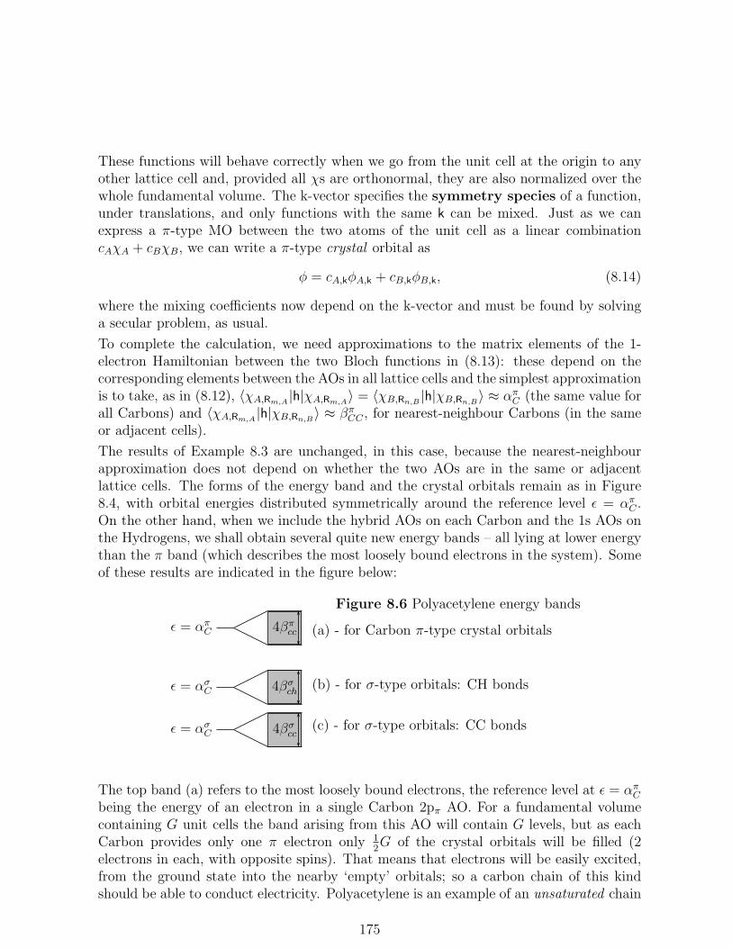
These functions will behave correctly when we go from the unit cell at the origin to anyother lattice cell and, provided all χs are orthonormal, they are also normalized over thewhole fundamental volume. The k-vector specifies the symmetry species of a function,under translations, and only functions with the same k can be mixed. Just as we canexpress a π-type MO between the two atoms of the unit cell as a linear combinationcAχA + cBχB, we can write a π-type crystal orbital as

φ = cA,kφA,k + cB,kφB,k, (8.14)

where the mixing coefficients now depend on the k-vector and must be found by solvinga secular problem, as usual.

To complete the calculation, we need approximations to the matrix elements of the 1-electron Hamiltonian between the two Bloch functions in (8.13): these depend on thecorresponding elements between the AOs in all lattice cells and the simplest approximationis to take, as in (8.12), 〈χA,Rm,A

|h|χA,Rm,A〉 = 〈χB,Rn,B

|h|χB,Rn,B〉 ≈ απ

C (the same value forall Carbons) and 〈χA,Rm,A

|h|χB,Rn,B〉 ≈ βπ

CC , for nearest-neighbour Carbons (in the sameor adjacent cells).

The results of Example 8.3 are unchanged, in this case, because the nearest-neighbourapproximation does not depend on whether the two AOs are in the same or adjacentlattice cells. The forms of the energy band and the crystal orbitals remain as in Figure8.4, with orbital energies distributed symmetrically around the reference level ǫ = απ

C .On the other hand, when we include the hybrid AOs on each Carbon and the 1s AOs onthe Hydrogens, we shall obtain several quite new energy bands – all lying at lower energythan the π band (which describes the most loosely bound electrons in the system). Someof these results are indicated in the figure below:

ǫ = απC 4βπ

cc

ǫ = ασC 4βσ

ch

ǫ = ασC 4βσ

cc

Figure 8.6 Polyacetylene energy bands

(a) - for Carbon π-type crystal orbitals

(b) - for σ-type orbitals: CH bonds

(c) - for σ-type orbitals: CC bonds

The top band (a) refers to the most loosely bound electrons, the reference level at ǫ = απC

being the energy of an electron in a single Carbon 2pπ AO. For a fundamental volumecontaining G unit cells the band arising from this AO will contain G levels, but as eachCarbon provides only one π electron only 1

2G of the crystal orbitals will be filled (2

electrons in each, with opposite spins). That means that electrons will be easily excited,from the ground state into the nearby ‘empty’ orbitals; so a carbon chain of this kindshould be able to conduct electricity. Polyacetylene is an example of an unsaturated chain

175

molecule: such molecules are of industrial importance owing to the electrical propertiesof materials derived from them.

Electrons in the lower bands, such as (b) and (c), are more strongly bound – with crystalorbitals consisting mainly of σ-type AOs, which lie at much lower energy. Figure 8.6 isvery schematic; the same reference level ασ

C is shown for the hybrid AOs involved in theCH bonds and the CC bonds (which should lie much lower); and the band widths areshown equal in all three cases, whereas the resonance integrals (β) are much greater inmagnitude for the AOs that overlap more heavily. So in fact such bands are much widerand may even overlap. On carefully counting the number of energy levels they containand the number of atomic valence electron available it appears that the crystal orbitalsin these lower energy bands are all likely to be doubly-occupied. In that case, as we knowfrom Section 7.4, it is always possible to replace the completely delocalized crystal orbitalsby unitary mixtures, without changing in any way the total electron density they give riseto, the mixtures being strongly localized in the regions corresponding to the traditionalchemical bonds.

There will also be empty bands at much higher energy than those shown in Figure 8.6,but these will arise from anti-bonding combinations of the AOs and are usually of littleinterest.

Other types of polymer chains

The polyacetylene chain (Figure 8.5) is the simplest example of an unsaturated polymer:the Carbons in the ‘backbone’ all have only three saturated valences, the fourth valenceelectron occupying a 2pπ orbital and providing the partial π bonds which tend to keepthe molecule flat. This valence electron may, however, take part in a 2-electron bond withanother atom, in which case all four Carbon valences are saturated and the nature of thebonding with its neighbours is completely changed. The simplest saturated polymers arefound in the paraffin series, which starts with methane (CH4), ethane (C2H6), propane(C3H8), and continues with the addition of any number of CH2 groups. Nowadays, theparaffins are usually called alkanes.

Instead of the ‘flat’ polyacetylene chains, which are extended by adding CH groups, thealkanes are extended by adding CH2 groups. The backbone is still a zig-zag chain ofCarbons, but the CC links are now single bonds (with no partial ‘double-bond’ character)around which rotation easily takes place: as a result the long chains become ‘tangled’,leading to more rigid materials. If the chain is kept straight, as a 1-dimensional lattice,the unit cell contains the repeating group indicated below in Figure 8.7 (where the unitcell contents are shown within the broken-line circle).

Figure 8.7 Repeating group (C2H4)Individual CH2 groups are perpendicular tothe plane of the Carbon chain (above it andbelow it)

(Carbons shown in black, Hydrogens in grey)

The first few alkanes, with few C2H4 groups and thus low molecular weight, occur as

176

gases; these are followed by liquid paraffins and then by solid waxes. But the chainlengths can become enormous, including millions of groups. The resultant high-densitymaterials are used in making everything from buckets to machine parts, while the lowerdensity products are ideal for packaging and conserving food. World production of thislow-cost material runs to billions of tons every year!

8.4 Some common 3-dimensional crystals

In Section 8.1 we introduced the idea of a crystal lattice, in one, two and three dimen-sions, along with the simplest model – in which an ‘empty lattice’ was just thought of asa ‘box’ containing free electrons. Then, in Section 8.2, we improved the model by definingthe crystal orbitals, as a generalization of the MOs used in Chapter 7 for discussingsimple molecules. Finally, in Section 8.3, we began the study of some ‘real’ systems bylooking at some types of ‘1-dimensional crystal’, namely polymer chains built mainly fromatoms of Hydrogen and Carbon. These simple chain molecules form the basis for mostkinds of plastics – that within the last century have changed the lives of most of us.

Most common crystals, however, are 3-dimensional and bring in new ideas which we arenow ready to deal with. The simplest of all (after solid Hydrogen) is metallic Lithium,a metal consisting of Lithium atoms, each with one valence electron outside a Helium-likeclosed shell. The atoms form a body-centred cubic lattice, with the unit cell indicatedbelow:

Figure 8.8 Indicating the unit cell of a body-centred cubic lattice

In the figure, atoms are shown as the shaded circles at the corners and centre of a cube.All lattice cells are identical, differing only by translations along the crystal axes; but theunit cell, containing only the two atoms shown with dark shading, ‘generates’ the wholecrystal by repetition in that way. Note that the atom at the middle of the cube has eightnearest neighbours, four on the top face of the cube and four on the bottom face: theatoms shown with light-gray shading ‘belong’ to the surrounding lattice cells.

Again we’ll use names A and B for the two atoms in the unit cell and suppose they areat positions rA and rB, relative to the origin of any cell. The ‘global’ position of A in a

177

lattice cell with origin at Rm will then be Rm + rA and similarly for B. Bloch functionscan be formed for each atom, just as in (8.13), which we repeat here;

φA,k(r) =1√G

3

∑

m

exp[ik·(Rm+rA)]χA,Rm(r), φB,k(r) =

1√G

3

∑

n

exp[ik·(Rn+rB)]χB,Rn(r).

(8.15)These functions are normalized, over the fundamental volume containing G3 cells, pro-vided all AOs (namely the χs) are normalized and orthogonal.

(Remember that χA,Rm(r) is an A-type AO centred on point rA in the lattice cell with

origin at Rm and similarly for χB,Rn(r). Remember also that the wave vector k is defined

in terms of the reciprocal lattice as

k = k1(2πb1) + k2(2πb2) + k3(2πb3)

and that with this definition the scalar products take the usual form with k·rA = k1(rA)1+k2(rA)2 + k3(rA)3, etc.)

The most general crystal orbital we can construct, using only the two Bloch functions(8.15), is

φ = cA,kφA,k + cB,kφB,k,

where the mixing coefficients follow from the usual secular equations. But matrix elementsbetween the Bloch functions may now depend on the wave vector k. Thus,

hAA = hBB = 〈φA,k|h|φA,k〉, hAB = 〈φA,k|h|φB,k〉.

Example 8.4 Reducing the matrix elements

The matrix elements of h between the Bloch functions may be reduced as follows. The diagonal elementbecomes, using (8.15),

hAA =1

G3

∑

m,n

exp[−ik · (Rm + rA)] exp[+ik · (Rn + rA)]

∫

χ∗A,Rm

hχA,Rndr,

where the minus sign in the first exponential arises from the complex conjugate of the function on theleft of the operator h, i.e. the function in the ‘bra’ part of the matrix element. The integral itself is α ifthe two functions are identical or β if they are nearest neighbours. Let’s do the summation over n first,holding m fixed. When the two AOs are identical, the exponential factor is unity and the integral factoris α. On doing the remaining summation, this result will be repeated G3 times – being the same for everylattice cell – and the normalizing factor will be cancelled. Thus hAA = αA, hBB = αB . This result doesnot depend at all on the wave vector k.

For the off-diagonal element we obtain, in a similar way,

hAB =1

G3

∑

m,n

exp[−ik · (Rm + rA)] exp[+ik · (Rn + rB)]

∫

χ∗A,Rm

hχB,Rndr,

but this contains the exponential factor

exp[ik · (Rn − Rm + rB − rA)] = exp ik · ρnm,

178

where ρnm = (Rn − Rm + rB − rA) is the vector distance from an atom of A-type, in lattice cell at

Rm, to one of B-type in a cell at Rn. The double summation is over all B-neighbours of any A atom,

so taking A in the unit cell at the origin and summing over nearest neighbours will give a contribution

(∑

n exp(ik·ρnm)×〈χA|h|χB〉. This result will be the same for any choice of the cell at Rm, again cancelling

the normalizing factor on summation. On denoting the structure sum by σAB(k), the final result will

thus be hAB = βABσAB(k), where βAB is the usual ‘resonance’ integral for the nearest-neighbour pairs.

Example 8.4 has given for the matrix elements of the 1-electron Hamiltonian, betweenBloch functions φA,k and φB,k,

hAA = αA, hBB = αB, hAB = βABσAB(k). (8.16)

Here, for generality, we allow the atoms or orbitals at rA and rB to be different; so laterwe can deal with ‘mixed crystals’ as well as the Lithium metal used in the present section.

The secular determinant is thus∣

∣

∣

∣

αA − ǫ βABσAB(k)βABσ

∗AB(k) αB − ǫ

∣

∣

∣

∣

= 0, (8.17)

where the ‘star’ on the second sigma arises because hBA is the complex conjugate of hAB

while the AOs are taken as real functions. This quadratic equation for ǫ has roots, foratoms of the same kind (αA = αB = α),

ǫk = α± βAB|σAB(k)|.

Since α and βAB are negative quantities, the states of lowest energy are obtained bytaking the upper sign. There will be G3 states of this kind, resulting from the solutionof (8.17) at all points in k-space i.e. for all values of k1, k2, k3 in the wave vector k =k1(2πb1) + k2(2πb2) + k3(2πb3). And there will be another G3 states, of higher energy,which arise on taking the lower sign. The present approximation thus predicts two energybands, of the kind displayed in Figure 8.6 for a 1-dimensional crystal (polyacetylene). Wenow look for a pictorial way of relating the energy levels ǫk within a band to the k-vectorof the corresponding crystal orbitals.

Brillouin Zones and Energy Contours

The results in Example 8.3, for a 1-dimensional crystal, are echoed in 2 and3 dimensions: a 3-dimensional crystal is considered in the next example.

Example 8.5 Bloch functions in three dimensions

A Bloch function constructed from AOs χn1n2n3at each lattice point Rn will be φ =

∑

n1,n2,n3cn1n2n3

χn1n2n3

and we try cn1n2n3= exp i(n1θ1 + n2θ2 + n3θ3).

Each factor cn = einθ will be periodic within the fundamental volume of G lattice cells in each directionwhen θ = 2πκ/G, κ being an integer. So the general AO coefficient will be

cκ1κ2κ3

n1n2n3= exp[2πi(n1κ1 + n2κ2 + n3κ3)/G],

179

where the three quantum numbers κ1, κ2, κ3 determine the state; and the energy follows, as in Example8.3, from the difference equation (in nearest neighbour approximation). Thus, the Bloch orbital energybecomes a sum of three terms, one for each dimension:

ǫκ1κ2κ3= α+ 2β1 cos(2πκ1/G) + 2β2 cos(2πκ2/G) + 2β3 cos(2πκ3/G).

In terms of the wave vector k and its components in reciprocal space, the 3-dimensionalBloch function and its corresponding ǫk can now be written, assuming all atoms have thesame α and all nearest-neighbour pairs have the same β,

φk =∑

n

exp(ik · Rn)χn, ǫk = α + 2β cos 2πk1 + 2β cos 2πk2 + 2β cos 2πk3, (8.18)

where χn is short for the AO (χn1n2n3) in the lattice cell at Rn = n1a1 + n2a2 + n3a3.

To get a simple picture of how ǫk depends on the k-vector components let’s take a squarelattice with only one AO per unit cell. In this 2-dimensional case the energy formula in(8.18) contains only the first two terms and can be written alternatively (simple trigonom-etry – do it!) as ǫk = α + 4β cos π(k1 + k2) cos π(k1 − k2). On taking the ‘fundamentalvolume’ to contain numbered lattice cells going from −1

2G to + 1

2G in each direction, the

G2 states will correspond to k1 and k2 each in the range (−12,+1

2). We can then define a

central zone in k-space by taking 2πb1 and 2πb2 as coordinate axes, along which to plotvalues of k1 and k2. This is the Brillouin zone in the following Figure 8.9:

k112−1

2

k2

12

−12

Figure 8.9 Zones in k-space

Brillouin zone bounded by the

broken line contains G2 states

(k1, k2 each in range (−12 ,+

12))

The formula ǫk = α + 4β cos π(k1 + k2) cos π(k1 − k2), obtained from (8.18) in the 2-dimensional case, then shows that the energy rises from a minimum α + 4β at the zonecentre (where k1 = k2 = 0) to a maximum α − 4β at the zone corners. The ‘top’ and‘bottom’ states thus define an energy band of width 8β.

Near the bottom of the band (β being negative), k1 and k2 are small and expanding thecosines in (8.18) gives the approximation (get it!)

ǫk = α + 4β − 4π2β(k 21 + k 2

2 ) + ... (8.19)

180

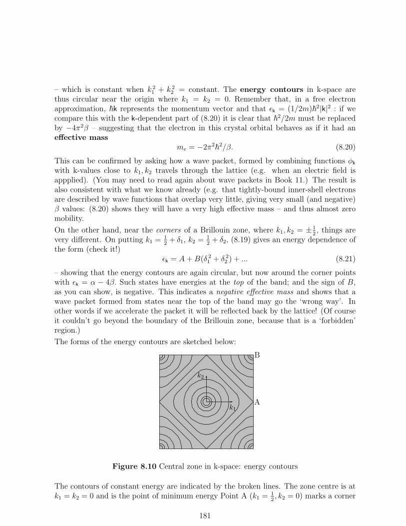
– which is constant when k 21 + k 2

2 = constant. The energy contours in k-space arethus circular near the origin where k1 = k2 = 0. Remember that, in a free electronapproximation, ~k represents the momentum vector and that ǫk = (1/2m)~2|k|2 : if wecompare this with the k-dependent part of (8.20) it is clear that ~2/2m must be replacedby −4π2β – suggesting that the electron in this crystal orbital behaves as if it had aneffective mass

me = −2π2~2/β. (8.20)

This can be confirmed by asking how a wave packet, formed by combining functions φk

with k-values close to k1, k2 travels through the lattice (e.g. when an electric field isappplied). (You may need to read again about wave packets in Book 11.) The result isalso consistent with what we know already (e.g. that tightly-bound inner-shell electronsare described by wave functions that overlap very little, giving very small (and negative)β values: (8.20) shows they will have a very high effective mass – and thus almost zeromobility.

On the other hand, near the corners of a Brillouin zone, where k1, k2 = ±12, things are

very different. On putting k1 =12+ δ1, k2 =

12+ δ2, (8.19) gives an energy dependence of

the form (check it!)ǫk = A+B(δ 2

1 + δ 22 ) + ... (8.21)

– showing that the energy contours are again circular, but now around the corner pointswith ǫk = α − 4β. Such states have energies at the top of the band; and the sign of B,as you can show, is negative. This indicates a negative effective mass and shows that awave packet formed from states near the top of the band may go the ‘wrong way’. Inother words if we accelerate the packet it will be reflected back by the lattice! (Of courseit couldn’t go beyond the boundary of the Brillouin zone, because that is a ‘forbidden’region.)

The forms of the energy contours are sketched below:

A

B

k1

k2

Figure 8.10 Central zone in k-space: energy contours

The contours of constant energy are indicated by the broken lines. The zone centre is atk1 = k2 = 0 and is the point of minimum energy Point A (k1 =

12, k2 = 0) marks a corner

181

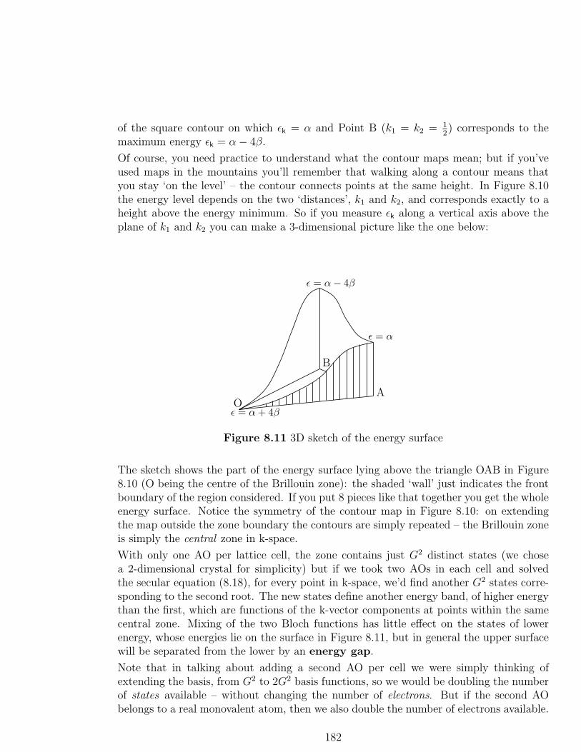
of the square contour on which ǫk = α and Point B (k1 = k2 = 12) corresponds to the

maximum energy ǫk = α− 4β.

Of course, you need practice to understand what the contour maps mean; but if you’veused maps in the mountains you’ll remember that walking along a contour means thatyou stay ‘on the level’ – the contour connects points at the same height. In Figure 8.10the energy level depends on the two ‘distances’, k1 and k2, and corresponds exactly to aheight above the energy minimum. So if you measure ǫk along a vertical axis above theplane of k1 and k2 you can make a 3-dimensional picture like the one below:

O

ǫ = α− 4β

B

ǫ = α

A

ǫ = α+ 4β

Figure 8.11 3D sketch of the energy surface

The sketch shows the part of the energy surface lying above the triangle OAB in Figure8.10 (O being the centre of the Brillouin zone): the shaded ‘wall’ just indicates the frontboundary of the region considered. If you put 8 pieces like that together you get the wholeenergy surface. Notice the symmetry of the contour map in Figure 8.10: on extendingthe map outside the zone boundary the contours are simply repeated – the Brillouin zoneis simply the central zone in k-space.

With only one AO per lattice cell, the zone contains just G2 distinct states (we chosea 2-dimensional crystal for simplicity) but if we took two AOs in each cell and solvedthe secular equation (8.18), for every point in k-space, we’d find another G2 states corre-sponding to the second root. The new states define another energy band, of higher energythan the first, which are functions of the k-vector components at points within the samecentral zone. Mixing of the two Bloch functions has little effect on the states of lowerenergy, whose energies lie on the surface in Figure 8.11, but in general the upper surfacewill be separated from the lower by an energy gap.

Note that in talking about adding a second AO per cell we were simply thinking ofextending the basis, from G2 to 2G2 basis functions, so we would be doubling the numberof states available – without changing the number of electrons. But if the second AObelongs to a real monovalent atom, then we also double the number of electrons available.

182

Many of the physical properties of real 3-dimensional crystals, such as the way theyconduct heat and electricity, depend strongly on the highest occupied electronic states;so it is important to know how the available states are filled. Every crystal orbital canhold only two electrons, of different spin (Pauli Principle), so with only one monovalentatom per lattice cell there would be 2G3 states available for the G3 valence electrons: thelowest energy band would be only half full and the next band would be completely empty.The crystal should be a good conductor of electricity, with electrons easily excited intoupper orbitals of the lower band; and the same would be true with two monovalent atomsper cell (4G3 states and 2G3 electrons). On the other hand, with two divalent atoms percell there would be 4G3 valence electrons available and these would fill the lower energyband: in that case conduction would depend on electrons being given enough energy tojump the band gap.

Some mixed crystals

Even simpler than metallic Lithium, is Lithium Hydride LiH, but the molecule doesnot crystallize easily, forming a white powder which reacts violently with water – all verydifferent from the soft silvery metal! On the other hand, Lithium Fluoride forms niceregular crystals with the same structure as common salt (Sodium Chloride, NaCl); theyhave the face-centred cubic structure, similar to that of the metal itself except that theFluorine atoms lie at the centres of the cube faces instead of at the cube centre.

Salts of this kind are formed when the two atoms involved (e.g. Li and F; or Na and Cl)are found on opposite sides of the Periodic Table, which means their electrons are weaklybound (left side) or strongly bound (right side). You will remember from Section 6.2 thatwhen the α-values of the corresponding AOs differ greatly the energy-level diagram for adiatomic molecule looks very different from that in the homonuclear case where the twoatoms are the same: in LiF for example, using A and B to denote Fluorine and Lithium,the lowest-energy MO (Figure 6.3) has ǫ1 ≈ αA while its antibonding partner has the muchhigher energy ǫ2 ≈ αB. The corresponding diatomic MOs, in the same approximation, areφ1 ≈ χA and φ2 ≈ χB, as you can confirm (do it!) by estimating the mixing coefficientsin φ ≈ cAχA + cBχB. In other words, the lowest-energy MO is roughly the same as theAO on the atom of greater electron affinity – meaning with the greater need to attractelectrons. When the MOs are filled with electrons (2 in each MO) the Fluorine will grabtwo of the valence electrons, leaving the Lithium with none. The bonding between thetwo atoms is then said to be ionic, the Fluorine being pictured as the negative ion F−

and the Lithium as the positive ion Li+. In that way both atoms achieve a closed-shell

electronic structure in which their valence orbitals are all doubly occupied. The Fluorine,in particular, looks more like the inert gas Neon, at the end of this row in the PeriodicTable.

When the salts form crystals similar considerations apply: the electronic structure ofthe crystal may be described by filling the available crystal orbitals, written as linearcombinations of Bloch functions, and the mixing coefficients could be calculated by solvinga set of secular equations at every point in k-space. But in the case of ionic crystals suchdifficult calculations can be avoided: looking ahead, we can guess that the Fluorine AO

183

coefficients in the crystal orbitals will come out big enough to justify a picture in whichthe Fluorine has gained an electron, becoming F−, while the Lithium has in effect lostits valence electron to become Li+. In this way we come back to the ‘classical’ picture ofionic crystals, put forward long before the development of quantum mechanics!

The unit cell in the LiF crystal, well established experimentally by X-ray crystallography,has the form shown below.

Figure 8.12 Fluorine ions (F−) in the LiF unit cell

Only the positions of the Fluorine ions, which are much bigger than the Li+ ions, areindicated in Figure 8.12, one being at a cube corner and three others being at the centersof three faces. This forms part of the unit cell ‘building block’, from which the wholecrystal can be constructed by adding similar blocks ‘face-to-face’ along the three axes. Asyou can see, the next block on the right will supply the missing F− ion on the right-handcube face, along with one at the bottom-right cube corner; and so it goes on if you addblocks in the other two directions (up/down and back/front). In that way every fluorineion finds its own position in the lattice, no two ‘wanting’ to occupy the same place. TheLithium positive ions are added to this face-centred lattice to give the electrically neutralLiF crystal, with 4 ions of each kind per unit cell. (Three of the Li+ ions are found at themid-points of the three cube edges that meet at the bottom-back corner, while the fourthis at the body-center of the cube; you might like to draw them in on Figure 8.12, alongwith all the other ions associated with that cubic cell in the crystal.)

So to do a quantum mechanical calculation, even at IPM level, it would be necessary totake account of 8 Bloch functions, solving an 8 × 8 secular problem at every point in k-space! and we’re lucky to be able to understand the structure of the crystal without havingto do such an enormous calculation. In the classical theory of ionic crystals we simplypicture the crystal as an array of negatively and positively charged spheres attracting eachother according to Coulomb’s inverse-distance law. But what stops the ions all collapsinginto each other to make all distances zero and the total energy minus infinity? That’s theonly point at which quantum mechanics must be used – and then it’s enough to show howtwo closed-shell ions build up a strong repulsion as soon as their electron distributionsbegin to overlap. The classical picture works well if it is supposed that the energy of

184

repulsion between two neighbouring ions has the form Erep = B exp(r/ρ) where B andρ are constants and r is the distance between the ion centres. Usually the constants aregiven empirical values so as to reproduce experimental data such as the unit cell distancesand the total energy of the crystal. Even then the calculations are not simple, becausethe crystal contains millions of ions and care must be taken with convergence as moreand more ions are included; but they are by now standard and give a good account ofcrystal properties. So let’s now look ar something really new!

8.5 New materials

A few years ago the Nobel Prize in Physics 2010 was awarded jointly to two Russians,Andre Geim and Konstantin Novoselov, for their groundbreaking experimental work onthe two-dimensional material graphene. Since then, thousands of scientific papers onthis material and its remarkable properties have been published in all the world’s leadingjournals. Graphene seems likely to cause a far bigger revolution in Science and Technologythan that made by the discovery of plastics – and yet all the underlying theory was knownmore than 50 years ago and can be understood on the basis of what you’ve done so far.

A crystal of solid graphite, which contains only Carbon atoms lying on a 3-dimensionallattice, consists of 2-dimensional ‘sheets’ or ‘layers’, lying one on top of another. Eachlayer contains Carbons that are strongly bonded together, lying at the corners of a hexagonas in the benzene molecule, while the bonding between different layers is comparitivelyweak. Such a single layer forms the 2-dimensional crystal graphene, whose unit cell isshown in the figure 8.13 (left) along with that for the corresponding k-space lattice (right).Because graphene is so important it’s worth showing how easy it is to construct all weneed from very first principles.

Example 8.6 A bit of geometry – the hexagonal lattice

Of course you’ve been using simple vector algebra ever since Book 2, usually with a Cartesian basis inwhich a vector v = vxi + vyj + vzk is expressed in terms of its components relative to orthogonal unitvectors i, j, k. So this is the first time you meet something new: the basis vectors we need in dealing withthe graphene lattice are oblique though they can be expressed in terms of Cartesian unit vectors. Thus,in crystal space, Figure 8.13 (left), we can choose i, j as unit vectors pointing along AB and perpendicularto it (upwards). We then have

a1 = 12

√3 i− 1

2 j, a2 = 12

√3 i+ 1

2 j.

In reciprocal space (i.e. without the 2π factors), Figure 8.13 (right), we can define

b2 = 12 i+

12

√3 j, b1 = 1

2 i− 12

√3 j

where b2 and b1 are respectively (note the order) perpendicular to a1 and a2). Thus, a1 · b2 = a2 · b1 = 0.

On the other hand a1 · b1 = 14

√3 + 1

4

√3 = 1

2

√3 and a2 · b2 has the same value. As a result, any pair of

vectors u = u1a1 + u2a2 (in ‘a-space’) and v = v1b1 + v2b2 (in ‘b-space’) will have a scalar product

u · v = u1v1(a1 · b1) + u2v2(a2 · b2) = 12

√3(u1v1 + u2v2),

185

since the other terms are zero. We’d like to have a simpler result, like that for two vectors in an‘ordinary’ (rectangular Cartesian) vector space. And we can get it if we replace the basis vectors b1, b2by b∗1 = ( 12

√3)−1b1 and b∗2 = ( 12

√3)−1b2, for then the factors ( 12

√3) cancel out. When the vectors u and

v are written as u = u1a1 + u2a2 and v = v1b∗1 + v2a2, we find (check it!)

u · v = u1v1 + u2v2

– exactly as for any pair of vectors in a single rectangular Cartesian space.

Let’s collect the two sets of basis vectors obtained in Example 8.6: the a-set define the‘real’ (‘crystal’) space, while the b∗-vectors define the reciprocal space, which is set uponly for mathematical convenience!

a1 =12

√3 i− 1

2j, a2 =

12

√3 i+ 1

2j

b∗1 = (√3)−1i− j, b∗2 = (

√3)−1i+ j. (8.22)

Thus,

a1 · b∗1 = (a2 · b∗2) = 1

but we still have a1 · b∗2 = a2 · b∗1 = 0. So for any two vectors, u, v, the first expressed incrystal space and the second in reciprocal space, we have

(u1a1 + u2a2) · (v1b∗1 + v2b∗2) = (u1v1 + u2v2)

– just as if the two vectors belonged to an ‘ordinary’ Cartesian space.

Now we know that the vectors set up in (8.22) have the properties we need, we can lookagain at Figure 8.13, which shows how they appear in the graphene crystal space andcorresponding k-space lattices:

a2

a1

A B

2πb∗2

2πb∗1

Figure 8.13 Crystal lattices and some unit cells (see text)

186

The left-hand side of Figure 8.13 shows part of the lattice in crystal space; one cell, theunit cell, contains Carbon atoms at A and B and is lightly shaded. The basis vectors a1and a2 are shown as bold arrows. The right-hand side shows part of the correspondinglattice in k-space: the basis vectors 2πb1 and 2πb2 are each perpendicular (respectively)to a2, a1 and define a unit cell (lightly shaded) in k-space. The central zone in k-spaceis hexagonal (shown in darker shading) and is made up from 12 triangular pieces, one ofwhich is shown, all equivalent under symmetry operations. You can imagine the 12 piecescome from the unit cell by ‘cutting it into parts’ and sliding them into new positions tofill the hexagon.

What we want to do next is to calculate the energy ǫ as a function of the coordinates(k1, k2) in k-space; then we’ll be able to sketch the energy contours within the unit cellor the equivalent central zone.

Calculation of the energy surfaces

As in dealing with aromatic hydrocarbons, where the highest energy MOsare built up from π-type AOs and serve to describe electrons moving inan effective field, provided by a flat σ-bonded ‘framework’, the first ap-proximation to calculations on a single graphite layer will start from thismodel. Again, with only two atoms in the unit cell, we shall need to solve asecular problem at every point in k-space to determine approximations tothe crystal orbitals. And when we express these 1-electron crystal orbitalsas linear combinations of Bloch functions in the form

φ(k) = cA,kφA,k + cB,kφB,k, (8.23)

the optimum approximation will follow from the secular equation∣

∣

∣

∣

hAA(k)− ǫ hAB(k)hBA(k) hBB(k)− ǫ

∣

∣

∣

∣

= 0, (8.24)

The matrix elements are between Bloch functions, namely φA,k, φB,k, wherefor example

φA,k =1

G

∑

m

exp[ik · (rA + Rm)]χA,Rm

and χA,Rmis the AO at point rA = (1/3)a1 + (1/3)a2 in the lattice cell at

Rm.

They can be reduced to those between the AOs as follows:

hAA =1

G2

∑

Rm

∫

χ∗A,Rm(r)hχA,Rm

(r)dr = 〈χA|h|χA〉,

187

with an identical result for hBB. (Note that 〈χA|h|χA〉 is for the A-atom inthe unit cell at the origin and that the summation is over G2 equal latticecells.) These diagonal matrix elements are independent of k :

hAA = 〈χA|h|χA〉, hBB = 〈χB|h|χB〉. (8.25)

The off-diagonal element, however, does depend on k :

hAB(k) =1

G2

∑

Rm,Rn

exp[ik · (rB + Rn − rA − Rm)]

∫

χ∗A,Rm(r)hχB,Rn

(r)dr.

We can make this look simpler by putting Rn + rB − rA = ρn, which is thevector that goes from atom at A in the unit cell at Rm = 0 to the atom atB in the lattice cell at Rn. Again there are G2 identical terms in the doublesum and the final result is thus

hAB(k) =∑

n

exp(ik · ρn)〈χA,0|h|χB,Rn〉. (8.26)

The summation in the last equation can be broken into terms for A-atomsand B-atoms in the same or adjacent cells (nearest neighbours) and then inmore distant cells (second and higher order neighbours). Equation (8.26)may thus be written

hAB(k) = h1σ1(k) + h2σ2(k) + ...,

where the terms rapidly get smaller as the A- and B-atoms become moredistant. Here we’ll deal only with the first approximation, evaluatingh1σ1(k) for nearest-neighbour contributions to σ1(k). We imagine atom Afixed and sum over the nearest B-type atoms; these will be B, in the samecell as A, and atoms at points B′ and B′′ in adjacent cells to the left, onelower for B′ and one higher for B′′. (Study carefully Figure 8.13, where youwill see B′ is at the lower right corner of the next hexagon, while B′′ isat its upper right corner.) The vector positions of the three B-atoms aregiven in terms of the Cartesian unit vectors i, j, by

rB = (2l)i+ 0j, rB′ = 12l i− 1

2

√3l j rB′′ = 1

2l i+12

√3l j,

where l = 1/√3 is the side-length of the hexagon. Their positions relative

to atom A are thus

rB = l i+ 0j, rB′ = −12l i− 1

2 j, rB′′ = −12 li+

12 j,

188

or, in terms of the a-vectors given in (8.22).

These are the corresponding ρ-vectors in (8.26); namely

ρB = (a1 + a2)/3, ρB′ = (1/3)a1 − (2/3)a2, ρB′′ = −(2/3)a1 + (1/3)a2.(8.27)

The contributions to the nearest-neighbour structure sum σ(k) arise fromatoms at the lattice points B, B′, B′′ (from now on we drop the ‘1’ subscript,standing for first neighbours) and thus give

σ(k) = exp(ik · ρB) + exp(ik · ρB′) + exp(ik · ρB′′).

To evaluate these contributions, which all involve scalar products betweenvectors in ‘real’ space and those in k-space, we must remember that thelatter contain a factor of 2π along with the reciprocal space basis vectorsb∗1, b

∗2. In fact, any v · k will take the usual form

v · k = 2π(v1k1 + v2k2).

On substituting the ρ-vectors given in (8.27) and using this last result, weobtain finally

σ(k) = [exp(2πi/3)(k1+k2)+exp(2πi/3)(k1−2k2)+exp(2πi/3)(−2k1+k2).(8.28)

The energy of the crystal orbitals ǫ, as a function of k, follows from thesecular equation (8.24). The diagonal matrix elements of the Hamiltonianh, given in (8.25), become (with the usual notation) hAA = hBB = α, whilethe off-diagonal element (8.26) becomes hAB(k) = βσ(k), β being the usual‘resonance integral’. The energy eigenvalues ǫ(k) are finally

ǫ(k) = α± β√

σ(k)σ∗(k), (8.29)

where the upper sign gives the lower -energy solution (that of a bondingorbital), since β is a negative quantity.

The squared modulus of the structure sum σ(k) in the energy expression(8.29) has the form

σ(k)σ∗(k) = (exp iθ1+exp iθ2+exp iθ3)× (exp−iθ1+exp−iθ2+exp−iθ3),

189

where

θ1 = (2π/3)(k1 + k2), θ2 = (2π/3)(k1 − 2k2), θ3 = (2π/3)(−2k1 + k2).

If you do the multiplication and note the properties of the exponentialsyou should find

σ(k)σ∗(k) = 3 + 2 cos 2π(k1) + 2 cos 2π(k2) + 2 cos 2π(k1 + k2)

and hence

ǫ(k) = α± β√

3 + 2 cos 2π(k1) + 2 cos 2π(k2) + 2 cos 2π(k1 + k2). (8.30)

To get the coordinates (k1, k2) of points in k-space we first draw the hexag-onal Brillouin zone, indicating the basis vectors b∗1, b

∗2. Note that k1, k2 are

the coefficients of b∗1, b∗2 in the k-vector. The result is shown in Figure 8.14

below (next page), where the end points of some particular k-vectors aremarked with bold dots. The other diamond-shaped areas are the adjacentcells in k-space.

The higher of the two bold dots is a K-point (corner point of the hexag-onal filled zone), while the lower is an M-point (mid-point of a side). Tocalculate the corresponding energies we must change to reciprocal-spacecoordinates, k1, k2, which go with the basis vectors b∗1, b

∗2.

In fact, the coefficients of b∗1 and b∗2 are, apart from the missing 2π factor,the components of the properly scaled k-vector, denoted by k1 and k2.

The following picture shows the central zone in k-space and indicates, withbold dots, two of the most important points (a K-point and an M-point).

190

2πb∗2

2πb∗1

Figure 8.14 Filled zone in k-space (see text)

You can find the energy value at any point in k-space, using the energyexpression (8.30) For example, at the centre of the hexagonal Brillouinzone k1 = k2 = 0 and (8.30) gives for ǫ(k) the value

α± β√

3 + 2 cos 2π(k1) + 2 cos 2π(k2) + 2 cos 2π(k1 + k2),

In other words, ǫ = α± β√9 = α± 3β. The upper sign gives the absolute

minimum ǫ = α+ 3β on the energy surface, while the lower sign gives thepositive maximum energy for orbitals in a second energy band.

At the M-point on the right-hand side you should find k1 = k2 = (3/4) andthis leads to, on using (8.30),

ǫ(k) = α± β√

3 + 2 cos 2π(3/4) + 2 cos 2π(3/4) + 2 cos 2π(3/2).

The result is thus ǫ = α + β√3 + 0 + 0− 2 = α + β at an M-point in

the central Brillouin zone. Now let’s turn to the general form of ǫ(k1, k2)throughout the zone:

Energy contours in the lowest-energy Brillouin zone

By evaluating (8.30) at a large number of points in k-space we can draw

191

in the contour lines on which ǫ(k) is constant. This is of course a tediousjob, but the results look nice and are sketched in the figure that follows.

2πb∗2

2πb∗1

Figure 8.15 Some energy contours in the filled zone (schematic)

The outer hexagon in Figure 8.15 shows the boundary (in k-space) of thelowest-energy Brillouin zone, which contains G2 1-electron states (see text).With two Carbons per unit cell, these are filled with the 2G2 π-electronsthey provide. Beyond the boundary, there begins the next zone – contain-ing orbitals that are normally empty. The energy contours are indicated bybroken lines and the corner-points (K-points) are marked with bold dots.

Notice that around the centre of the filled zone, where the energy has theabsolute minimum value ǫ = α+3β, the contours are almost perfect circles;but when the energy approaches ǫ = α + β the contour becomes a perfecthexagon, whose sides join the mid-points (the M-points) of the hexagonalboundary of the filled zone, and here the surface becomes ‘flat’, all points

192

on the hexagon having the same energy as at the M-point. After that, theenergy approaches the value ǫ = α, the highest energy level in the filledzone, but this is found only at the K-points and close to them – where thecontours again become roughly circular. At these points, something veryunusual happens: the energy surface is just touched by the lowest-energypoints of the next energy surface, whose orbitals have energies going fromǫ = α up to the maximum ǫ = α − β. At all other points there is a gapbetween the lower and upper surfaces.

It is this strange fact that gives graphene its unique properties.

The π electrons serve mainly to ‘stiffen’ the sigma-bonded framework ofCarbon atoms and to give the material the unique properties that arisefrom the touching of the two energy surfaces. The Carbon-Carbon bonds ingeneral can be difficult to break, especially when they form a 3-dimensionalnetwork that can’t be pulled apart in any direction without breaking verymany bonds. This is the case in crystals of diamond, where every Carbonforms tetrahedral bonds with its four nearest neighbours, as in Figure 7.7.(Remember that diamonds – which contain only Carbon atoms – are usedin cutting steel!) But in graphite the Carbons have the rare property offorming separate layers, held together only by very weak bonds – whichallow them to slide over one another, or to be ‘peeled off’ as sheets ofgraphene.

The great strength of graphene sheets is often called the “Cat’s Cradle”property, because a single sheet – one atom thick and weighing almostnothing! – would support the weight of a sleeping cat!

More useful properties arise from the limited contact (in k-space) betweenthe filled and empty electronic bands. When the lowest-energy band isfilled and separated from the next band above it by an energy gap greaterthan (3/2)kT (which is the average energy of a particle in equilibrium withits surroundings at temperature T ◦ K – as you may remember from Book5) an electron with energy at the top of the filled band is unable to jumpacross the gap into an orbital of the empty band, where it will be ableto move freely. But at the K-points in graphene the energy gap is zeroand some electrons will be found in the conduction band where they arefree to conduct electricity. In fact, graphene is a perfect semiconductor,

193

whose conductivity starts at zero, when it is cold, but rises rapidly asthe temperature increases. You know how valuable semiconductors havebecome nowadays, when they form the vital parts of so many electronicdevices such as radios and computers.

Such properties are revolutionizing not only whole fields of experimentalPhysics and Technology, but also large parts of Chemistry and Biology.Tiny sheets of graphene can be wound into ‘tubes’ so small that they cancarry single atoms from one place to another, opening up new fields of‘molecular engineering’.

“Looking back – ” and “Index” to follow (10 May 2014)

194