Quantitative Trait Loci for the Circadian Clock in Neurospora crassa

1

Quantitative Trait Loci for the Circadian Clock in Neurospora crassa

Tae-Sung Kim*, Benjamin A. Logsdon†, Sohyun Park*, Jason G. Mezey†, Kwangwon Lee*1

*Department of Plant Pathology, Cornell University, Ithaca, NY 14853. †Department of

Biological Statistics and Computational Biology, Cornell University, Ithaca, NY 14853

Genetics: Published Articles Ahead of Print, published on October 18, 2007 as 10.1534/genetics.107.077958

2

Running head: Neurospora clock QTL

Key words: circadian rhythms, period, phase, composite interval mapping, Bayesian QTL

mapping

1 corresponding author

Kwangwon Lee.

Department of Plant Pathology

201 Bradfield Hall

Cornell University

Ithaca NY 14853

Phone: 607-255-5924

Fax: 607-255-8835

E-mail: [email protected]

3

ABSTRACT

Neurospora crassa has been a model organism for the study of circadian clocks for the past

four decades. Among natural accessions of N. crassa, there is significant variation in clock

phenotypes. In an attempt to investigate natural allelic variants contributing to quantitative

variation, we used a Quantitative Trait Loci (QTL) mapping approach to analyze three

independent mapping populations whose progenitors were collected from geographically isolated

locations. Two circadian clock phenotypes, free running period and entrained phase, were

evaluated in the 188 F1 progeny of each mapping population. To identify the clock QTL, we

applied two QTL mapping analyses: composite interval mapping (CIM) and Bayesian multiple

QTL analysis (BMQ). When controlling false positive rates 05.0≤ , BMQ appears to be the more

sensitive of the two approaches. BMQ confirmed most of the QTL from CIM (18 QTL) and

identified 23 additional QTL. While 13 QTL co-localize with previously identified clock genes,

we identified 30 QTL that were not linked with any previously characterized clock genes. These

are candidate regions where clock genes may be located and are expected to lead to new insights

in clock regulation.

INTRODUCTION

Biological rhythms with about a 24 hour period have been found in all forms of life from

bacteria to humans (BELL-PEDERSEN et al. 2005; FELDMAN and HOYLE 1973; LAKIN-THOMAS

2006; SCHIBLER 2006; STANEWSKY 2003; YOUNG and KAY 2001). The availability of powerful

genetic analysis tools and the easily assayable clock phenotype in Neurospora crassa has made

4

the system one of the most successful model organisms for dissecting the circadian clock using a

forward genetics approach (DUNLAP and LOROS 2004; FELDMAN and HOYLE 1973; LOROS and

DUNLAP 2001). Mutant screens for clock genes have focused on mutants with altered period or

arrhythmic phenotypes caused by a single mutation inherited through Mendelian segregation

(FELDMAN and HOYLE 1973). The most interesting gene discovered in these mutant screenings

is frequency (frq). Different mutant alleles of frq could cause a long period, short period or

arrhythmic phenotype (DUNLAP and LOROS 2004; FELDMAN and HOYLE 1973; LOROS and

DUNLAP 2001). This finding led to the proposal that a single gene could function as a “state

variable” for the circadian oscillator (ARONSON et al. 1994).

Cloning and characterizing the frq gene significantly advanced our molecular understanding of

eukaryotic circadian oscillators (DUNLAP and LOROS 2006; LIU and BELL-PEDERSEN 2006).

Despite extensive molecular characterization of frq and other known clock genes in N. crassa,

there is still no comprehensive understanding of the Neurospora circadian clock. Furthermore,

with advances in our understanding of the molecular structure of Neurospora clocks, it is

apparent that the circadian clock is more tightly linked to other cellular machinery than

speculated previously (BELL-PEDERSEN et al. 2001). For example frq-less oscillators (FLO)

coupled to other oscillators in the cell have been proposed (LAKIN-THOMAS 2006). Currently, we

know very little about the genetic basis of these loosely defined oscillators (DUNLAP and LOROS

2006).

The conventional forward genetics approach is limited in two ways; it cannot uncover genetic

loci with subtle clock phenotypes or those associated with essential cellular functions (HE et al.

2005; MACKAY 2001a). Furthermore, most of the genetic screening done previously was focused

on identifying period determinants. Thus, just a handful of genetic loci have been characterized

5

that are responsible for other clock properties such as entrained phase or temperature

compensation. Here, we explore an alternative strategy for detecting novel genetic loci affecting

the N. crassa circadian clock.

Within natural populations there reside important clues to genetic variation, which are vital in

unraveling the mysteries of gene function (ALONSO-BLANCO and KOORNNEEF 2000). Identifying

the molecular components and characterizing the molecular mechanisms of the natural variations

will provide us novel insights into molecular mechanisms of complex circadian traits.

Quantitative genetics techniques have been utilized successfully over the past decade to describe

how alleles genetically interact with each other to modulate the circadian traits as well as to

isolate new loci in the same pathway (SHIMOMURA et al. 2001). Quantitative genetics is an

extension of fundamental Mendelian principles to polygenic traits (phenotypes encoded by

multiple loci). Much of the phenotypic variation seen in natural populations is due to multiple

loci contribute to phenotypic variation (ALONSO-BLANCO and KOORNNEEF 2000). Each

quantitative trait locus has a relatively small effect on the phenotype. The combination of

genomic sequence, new molecular marker technologies and sophisticated mapping algorithms

has made it possible to utilize natural variation in combination with QTL analysis to dissect

complex traits down to a single sequence polymorphism (DOERGE 2002; LANDER and SCHORK

1994). For circadian clock phenotypes, clock QTL have been identified in multiple organisms

including Arabidopsis and in mice (DARRAH et al. 2006; EDWARDS et al. 2006; EDWARDS et al.

2005; MICHAEL et al. 2003; SUZUKI et al. 2001; SWARUP et al. 1999).

There have been no reports on QTL analysis for Neurospora circadian clock phenotypes. This

may have been due to technical barriers. The most common assay to measure the Neurospora

clock has been the race tube assay. As a result of circadian clock-controlled asexual

6

development, Neurospora produces orange spores. These dense orange colored spores create a

“banding” phenotype in a long glass tube or “race tube” (LOROS and DUNLAP 2001). This easily

detected clock phenotype made the Neurospora circadian rhythm an attractive system for genetic

studies. All laboratory Neurospora strains used in clock studies contain a useful mutation band,

bd (BELDEN et al. 2007; SARGENT and WOODWARD 1969). This mutation allows a robust

conidial banding pattern even in the high CO2 environment of the race tube culture. In the wild

type strains without the bd mutation, the rhythmic asexual development of Neurospora in a race

tube is suppressed, which has been a major obstacle in clock study (SARGENT and KALTENBORN

1972). However, modified race assay have recently been developed that allows study of

Neurospora circadian clocks in natural accessions without the bd mutation in their genetic

background (BELDEN et al. 2007; PARK and LEE 2004).

The Neurospora system provides a unique opportunity to extend quantitative genetics to

molecular genomics due to its sequenced haploid genome (GALAGAN et al. 2003). Haploid

organisms provide multiple advantages in quantitative studies: 1) they can be maintained

clonally to allow large numbers of individuals to be assayed (thereby reducing error from

environmental effects); 2) genetic dominance does not contribute to the genetic variation; 3) a

permanent segregating population is available after the first generation; and, as in the case of

Neurospora, 4) the sexual cycle is short (DAVIS and PERKINS 2002). For these reasons,

Neurospora can serve as a valuable model organism for elucidating fundamental questions of

quantitative genetics for complex behaviors such as the circadian clock. In previous studies, we

found significant natural variation in clock phenotypes and known clock genes among 143

natural accessions of N. crassa (MICHAEL et al. 2007). By crossing these natural accessions, we

successfully produced linkage maps for three line-cross populations (KIM et al. 2007).

7

In this report, we describe the QTL analysis of the two clock phenotypes, period and entrained

phase using natural populations. In an effort to find natural genetic variations affecting the clock

phenotype efficiently, we employed two QTL analyses, composite interval mapping (CIM) and

Bayesian multiple QTL (BMQ) analysis in three independent mapping populations derived from

the natural accessions that were collected from geographically isolated areas. We expected that

QTL analyses using multiple populations would provide us additional insight on natural variation

of clock phenotypes. We predicted that we will find certain clock QTL in more than one

population. We hypothesized that these common QTL might play important role for ecological

adaptation. We also expected that analyzing multiple populations would give us meaningful

insight on how many QTL is involved in period, phase, and both phenotypes. Our results include

identification of 1) common QTL that are detected in more than one population, 2) population-

specific QTL, and 3) QTL that contribute to both period and phase phenotypes.

MATERIALS AND METHODS

Strains and growth conditions: Natural accessions, FGSC#3223, FGSC#4724, FGSC#4720,

FGSC#4715, FGSC#4825 and FGSC#2223, were obtained from Fungal Genetics Stock Center,

www.fgsc.net. F1 progenies from three crosses were obtained as previously described (DAVIS

2000). Detailed information on the parental strains in their estimated geographical origin and

circadian properties is summarized in Table 1. The germination rate of the cross varied

significantly between batches of spores. For example, we compared the 16 small batches of

ascospores of the same cross (N2 progeny) for their germination rate over a month period. The

germination rates ranged from 15 to 66%. Strains used in this study were cultured as previously

8

described (LEE et al. 2003). The overt clock phenotypes including period and phase were

measured utilizing the Inverted Race Tube Assay (PARK and LEE 2004).

Assessing phenotype: Race tubes were incubated in constant light (LL) for 12 hrs at room

temperature. After confirming normal mycelial growth in the race tube, tubes were transferred to

an I-36L Percival Scientific (Perry, IA) growth chamber and incubated an additional 12 hr under

LL. For all experiments, temperature was set at 25º. After the 24hr LL treatment, the light was

off for the rest of the experiment for the period measurement. The growing front was marked at

the light to dark transition and on the last day of experiment. In the race tube experiment for the

phase phenotype, the light condition was light12 hr: dark12 hr (LD) cycle. The growing front of

the culture in the race tube was marked every 24 hr at the time when the light to dark transition

occurred. The fluence rate was 250 µE/m2/s in LL. Light sources were white fluorescent bulbs

and incandescent bulbs (Osram Sylvania Inc.). In both period and phase experiments, tubes were

randomly positioned within the chamber to reduce the possibility of positional effects. In each

experiment, three replicates of each progeny were assayed. We repeated the experiment to

generate data from at least three biological replicates for each strain; sometimes, we were not

able to attain data from all three replicates in one experiment.

Period analysis: For the analysis of period phenotype, individual period estimates of F1

progenies of each population were produced after 4-5 days of consecutive conidial banding,

using the Fast Fourier Transform Nonlinear Least-Squares (FFTNLS) program (EDWARDS et al.

2005; PLAUTZ et al. 1997).

Phase analysis: The reference time for phase of each individual genotype/progeny was the

band center. Thus, the phase of each individual progeny was determined based on the time

elapsed to reach the band center within a day. Band center was visually determined by the spore

9

density. The time when cultures were transferred to the dark cycle is, by definition, CT12 (dusk).

Thus, in these experiments, the time in band center of each individual was calculated by the

following formula: zeitgeber (ZT) phase= (growth to band center/ overall growth) x 24+ 12. For

example, if conidial band occurs at 180 mm and total growth after light dark transition is 280

mm, ZT phase= 24 × (180/280) + 12 = 27.43. By convention, ZT is always expressed as less

than 24 ZT hr. For example, ZT phase 27.43 is expressed as ZT 3.43 (27.43 – 24) instead of ZT

27.43.

Genotyping and genetic map construction: The genotyping method and linkage group

analysis was done as described previously (CHO et al. 2000; SCHUELKE 2000; YU et al. 2006).

We also utilized the physical map information at the Broad Institute database,

http://www.broad.mit.edu/annotation/genome/neurospora/maps/Index.html.

Statistical analysis: QTL analysis was carried out on the mean value of free running period

and entrained phase in N2, N4 and N6 populations (Table 2). Markers with significant

segregation distortion (χ2 test, p=0.05) were disregarded. Composite Interval mapping (CIM) and

Bayesian QTL mapping (BMQ) were used to identify putative clock QTL.

CIM analysis: CIM analysis using the QTLCartographer v.2.5 (BASTEN et al. 2006) was

conducted with a walking speed of 0.5 and a window size of 3 cM under a forward and backward

regression model (probability into 0.01, probability out 0.1). To determine experimental type 1

error, 1,000 permutations were performed for period and phase phenotypes in three (N2, N4 and

N6) populations (CHURCHILL and DOERGE 1994). We defined the confidence interval as the

physical genome region above the threshold defined by these 1,000 permutations. This functional

confidence interval region was on average 10 cM or about 200-300 kilobase pair (kb) around the

genetic positions with the maximum Likelihood Ratio (LR) score. We searched for candidate

10

clock QTL genes in the genome region within confidence interval regions. LR critical values

ranged from 11 to 12 (P = 0.05) in all analyses. Additive effect estimates and percentages of

variance explained by the QTL were generated with Eqtl, testing hypothesis 10 and using model

6 from Zmapqtl. LR profiles for two circadian properties including free running period and

entrained phase in the three populations of our study are displayed in Figure 3, Figure 4 and

Table 3.

BMQ analysis: The BMQ approach uses a hierarchical modeling scheme in which at the “top”

level, each marker has a probability of being categorized into one of three classes: linked to a

QTL with a positive effect on (i.e. increases) the value of the phenotype ( +p ), linked to a QTL

with a negative effect on the phenotype ( −p ), and not linked to a QTL ( −−− pp+1 ) (ZHANG et

al. 2005). At the “bottom” level, the actual effects of QTL are defined in the usual way using a

linear model. The advantage of this hierarchical classification approach is that, with an

appropriate choice of prior for marker class hyper-parameters (ZHANG et al. 2005), we can

implement an efficient stochastic search in low-dimensional model subspaces. This avoids the

tendency to over-shrink estimates of QTL effects observed with other multi-QTL Bayesian

approaches (TER BRAAK et al. 2005; YI et al. 2003).

Following a previous report (ZHANG et al. 2005), we used a “spike and slab” prior (GEORGE

and MCCULLOCH 1993) which incorporates the assumption that most markers will not be linked

to a QTL. Thus, in our Bayesian classification framework, the probability that a marker is linked

to a QTL is reflected by the posterior probability distribution associated with the marker classes

+p and −p . We implemented the Gibbs sampler described in Zhang et al. (2005) to generate

samples from these posterior distributions. Marginal posteriors for both the additive effect (β)

11

and probabilities of categorization ( +p , −p ) were estimated by sampling 5000 iterations after an

initial burn in of 5000.

We considered the cumulative probability greater than 0.5 that the marker is in the +p ( −p )

class to determine whether a marker is linked to a QTL (hereafter we refer to this as the Posterior

Probability Threshold or PPT). This is a univariate version of the heat map summary provided in

Zhang et al. (2005) and reflects the probability that a marker has a greater than 50% chance of

being linked to a QTL.

QTL names were formulated in order of the name of the mapping population, the QTL method

used ("C" for CIM specific QTL and “B" for BMQ specific QTL, BC for the QTL detected both

by CIM and BMQ), the trait targeted (for example, “per” for period and “pha” for phase),

chromosome (chr.) number, and numeric numbers to differentiate QTL within a chr. For example,

N6CBper7-1 refers to 1st QTL located on chromosome VII, period phenotype in N6 that was

detected both by CIM and BMQ methods.

RESULTS

Period and phase analyses: We generated three F1 progeny derived from mapping parents

described in Table 1 to map QTL for two circadian phenotypes, free running period and light

entrained phase. Each mapping population was composed of 188 progeny derived from a cross

between two N. crassa natural accessions (Table 2). Continuous patterns of the distribution of

both circadian phenotypes in F1 progenies were observed in all three crosses, indicating that

inheritance of the circadian properties in N. crassa is polygenic (Figure 1 and Figure 2), which is

consistent with results with previous studies in other systems (DARRAH et al. 2006; EDWARDS et

12

al. 2006; EDWARDS et al. 2005; HOFSTETTER et al. 1995; HOFSTETTER et al. 1999; KERNEK et al.

2004; KOPP 2001; MAYEDA and HOFSTETTER 1999; SALATHIA et al. 2002; SUZUKI et al. 2001;

SWARUP et al. 1999; TOTH and WILLIAMS 1999; WELCH et al. 2005). The mean period lengths of

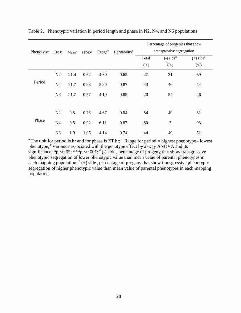
our mapping populations were 21.4 hrs, 21.7 hrs, and 21.7 in N2, N4, and N6 populations,

respectively (Table 2). The period of the parental lines of each population were approximately

similar to the mean values of the periods in the F1 progeny (Figure 1 and Table 2). The ranges of

the period length in N2, N4, and N6 were 4.55, 5.79, and 4.12 hr, respectively. The broad sense

of heritability (H2) of N. crassa clock phenotype was high in all populations, 0.62, 0.87 and 0.85,

which suggests phenotypic variation in the segregating populations was due to mostly genetic

effects.

Traditionally, the phase phenotype has been expressed in subjective hours, or zeitgeber (ZT)

hours (see Materials and Methods). In contrast to period, the means of the phase values among

progenies in different populations were different; the mean phase value in N2 and N4 was 0.5 ZT

hr, whereas, in N6 it was 1.6 ZT hr (Figure 2 and Table 2). The phase of the parental lines of N2

and N6 populations was close to the mean of the phase of the progenies. However, in the N4

population, 93% of N4 progeny were distributed toward the right side (+ side) of the mean value

of parental strains in the phase phenotype (Figure 2 and Table 2). The ranges of phase

distribution in N2, N4, and N6 were 4.7, 6.1, and 4.1 ZT hr, respectively. As observed in period

value, relatively high heritability in phase was also observed in each population; the heritabilities

of N2, N4 and N6 were 0.84, 0.87 and 0.74, respectively. There was no correlation between

period and phase under entrained environment within a population in all three populations

(supplemental data Figure 1 at http://www.genetics.org/supplemental).

13

Comparison of CIM and BMQ methods for clock QTL analyses: In an effort to pinpoint

the clock QTL and identify genetic elements responsible for subtle phenotypic variation in the N.

crassa clock efficiently, two independent QTL analysis methods (CIM and BMQ, see Materials

and Methods) were used.

In the BMQ approach, we considered a cumulative probability greater than 0.5 (Posterior

Probability Threshold or PPT) to determine whether a marker was linked to a QTL (Materials

and Methods). To assess the appropriate PPT cutoff when determining whether a marker was

linked to a QTL, we simulated QTL data using marker data from population N6. We defined

“neutral markers” as markers that are not linked to QTL (ZHANG et al. 2005). In our simulation

study we estimated the PPT level expected to minimize the number of false positives.

The results of the simulations are summarized in supplemental data Figure 2 at

http://www.genetics.org/supplemental. When there is no QTL, i.e. additive effects = 0, no

neutral marker had a PPT>0.01 (or < -0.01). When three QTL of equal effect spaced throughout

the genome are simulated, the PPT for neutral markers can be larger but the bulk of the truly

neutral markers still have a PPT<0.05. In fact, even as the effects of the simulated true QTL are

decreased to an additive effect of 0.25 (heritability of 0.13), only 1 neutral marker had a PPT >

0.05, showing PPT= 0.16 (supplemental data Figure 2 at http://www.genetics.org/supplemental).

Missing genotype data can increase the type I error rates for neutral loci when there are QTL

present as seen in supplemental data Figure 2 at http://www.genetics.org/supplemental, where

the distribution of PPT across neutral markers has greater outliers with smaller additive effects.

We therefore used PPT=0.17 as a cutoff for deciding whether markers were linked to QTL to

minimize false positive rates.

14

We also performed a simulation experiment with three pre-defined QTL (supplemental data

Figure 3 at http://www.genetics.org/supplemental). Note that neutral markers surrounding the

marker in strongest linkage disequilibrium with a QTL also have reasonably high PPT but that

the highest PPT occurs at the marker where the true QTL is positioned (supplemental data Figure

3 at http://www.genetics.org/supplemental). For a set of consecutive markers with PPT ≥ 0.17,

we therefore determined the marker with the greatest PPT to be linked to a QTL.

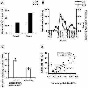
We detected twice the number of QTL from BMQ compared to that from CIM (Figure 5A).

BMQ identified all QTL that were found in CIM in both phenotypes of our study (Table 3,

Figure 5B) except two QTL (N6CPer7-2 and N6Cper7-3, Table 3). The peak positions on the

marker loci linked to significant QTL were highly consistent in the two methods (Figure 5B).

The ranges of the PPT were variable, spanning from 0.17 to 0.96 (supplemental data Figure 4 at

http://www.genetics.org/supplemental), in which the median value is 0.43 Average PPT for

QTL detected by both methods is significantly higher than the average PPT for QTL that were

detected only by BMQ (0.58 versus 0.30, Figure 5C). The LR score in CIM showed a highly

significant positive correlation with PPT in BMQ (Pearson’s correlation coefficient = 0.69

p<0.0001, Figure 5D). Hereafter, we ascribe all QTL with PPT values except for those two QTL

(N6CPer7-2 and N6Cper7-3) undetectable by BMQ.

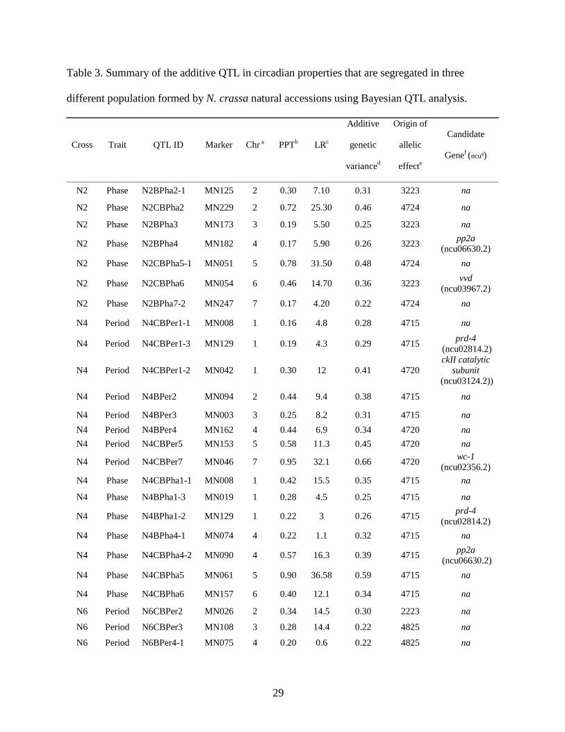
Clock QTL: From two statistical methods, we detected 43 QTL from three populations that

affect the two circadian clock properties, period and phase (Table 3). We detected a similar

number of QTL in two clock phenotypes per population; eight QTL in period and nine QTL in

phase per population (Table 3 and supplemental data Figure 5 at

http://www.genetics.org/supplemental) except the period phenotype in N2 where we did not

detect any significant QTL with either CIM or BMQ analyses.

15

We searched for candidate QTL genes around the detected clock QTL regions to see whether

previously characterized clock genes were localized with the clock QTL. We defined the

confidence interval region for the clock QTL by performing a permutation test (see Materials and

Method). We also developed wc-1 and vvd specific SSR markers as positive controls. This

strategy was based on the idea that one of the QTL may co-localize with these two key genes

(wc-1 in period, vvd in phase) in N. crassa clock regulation. Two QTL in period (N6Cper7-3 and

N4CBper7, Table 3 and Figure 3) and two QTL in phase (N2CBpha6 and N6CBpha6, Table 3

and Figure 4) co-localized with those clock gene-specific markers. In period QTL, in addition to

wc-1, we found several QTL that were linked to previously characterized genes involved in

period determination; the key clock gene frq and the genes involved in frq phosphorylation and

degradation. Candidate period QTL genes and phase QTL genes are listed in Table 3. Although,

these genes were known to influence phase of the N. crassa clock, the specific roles of theses

candidate genes for phase-determination have not been clearly studied except for vvd (ELVIN et

al. 2005; HEINTZEN et al. 2001). These results suggest that our QTL studies were concordant

with previous clock studies and give insight into the mechanism of N. crassa regulation,

especially in phase regulation. Nine (out of 16 QTL in period) and 16 QTL (out of 26 QTL in

phase) were characterized as unknown clock loci, which suggest there is a lot more to understand

about N. crassa circadian clock. Several QTL, especially in phase phenotype, with high

significance level are still uncharacterized, including N2Bpha5-1 (PPT=0.78, LR=35.5),

N2Bpha2 (PPT=0.72, LR=25.3) and N4Bpha5 (PPT=0.90, LR=35.8). The co-localized candidate

genes with QTL are also summarized in Table 3.

We wanted to estimate how many clock QTL were identified more than once in different

populations. Obviously, we could increase the chance of identifying all potential clock QTL by

16

increasing the number of mapping populations. However, for practical reasons, we chose to

characterize three independent line-cross populations. To avoid the over-estimation of the

number of clock QTL, we excluded the common QTL identified in different populations. We

found that there were no significant chromosome re-arrangements among N. crassa natural

isolates that we studied (KIM et al. 2007). Thus, we defined the common QTL as a QTL linked to

the same SSR marker in more than one population for the same phenotype regardless of their

relative genetic positions. Three QTL out of 16 QTL for the period phenotype and eight QTL out

of 27 QTL for the phase phenotype are common QTL (supplemental data Figure 6 at

http://www.genetics.org/supplemental). Thus, our data suggest that at least 13 different QTL

contribute to the period phenotype, and 19 different QTL contribute to the phase phenotype

respectively.

Lastly, we wanted to know how closely the period and entrained phase phenotypes were

genetically interrelated. To answer that question, we investigated how many QTL were

contributing both to period and phase phenotypes. Since we could not detect any period QTL in

N2, we excluded the comparison between the phase and period QTL in N2 population. Three

QTL in N4 and two QTL in N6 contribute to both in period and phase variations respectively

(Table 3 and supplemental data Figure 6 at http://www.genetics.org/supplemental). We also

found seven QTL that contribute to both period and phase variations when we consider all three

populations (Table 3 and supplemental data Figure 7 at http://www.genetics.org/supplemental).

This suggests that there are common genetic elements contributing for both period and phase

phenotypes.

DISCUSSION

17

Our study showed that fungal F1 populations can be employed as mapping populations for a

QTL study of circadian clock phenotypes. From the three independent F1 populations in our

study (N2, N4 and N6), a wide range of phenotypic transgressive segregation was observed in

both free running period and light entrained phase clock phenotypes. Since those phenotypes

shows high heritability consistently in the line-cross populations (average H2 = 0.79, standard

deviation=0.12) and the genome structure of two parental strains are so divergent (minimum

pair-wise dissimilarity= 0.91, supplemental data Figure 8 at

http://www.genetics.org/supplemental), the phenotypic transgressive segregations of the

phenotypes that are observed in those populations are presumably attributable to segregation of

the accumulated genetic variations between the parental strains.

Haploid organisms have an important advantage in constructing a mapping population; due to

the haploid nature of genome, one generation (F1) is enough to make a breeding population

similar to that of recombinant inbred line (RIL), where it takes at least 8-9 generations of selfing

in plant species or about 20 generations of full-sib mating for out- breeding animals. Size of

mapping population is the critical consideration when using a F1 population for QTL analysis.

Because there are so few meiotic events in a F1 population compared to RIL lines, a small

number of progeny can cause errors in estimating genetic distance and order. Hackett and

Broadfoot performed simulation studies to give a reasonable guess for the mapping population

size (HACKETT and BROADFOOT 2003). They investigated locus ordering performance in genetic

linkage map construction of double haploid (DH) population under the conditions where effects

of missing values, typing errors and distorted segregation are allowed (HACKETT and

BROADFOOT 2003). With 150 DH progeny, they concluded that a locus order spacing of 10 cM is

relatively insensitive to missing values as high as 20% and typing errors around 3%. In

18

agreement with their result, the order of mapped loci in our study is quite consistent with the

physical map (KIM et al. 2007). Furthermore, significant QTL associated with period and phase

variation were detected in a 10 cM resolution (Table 3).

The statistical power to detect meaningful QTL can be determined by many factors including

the size of the mapping population, the genome organization of the target organism, the

experimental designs for the mapping population, the types of molecular marker, the qualities of

phenotyping and genotyping analysis and method of statistical analysis (ZENG 1994; ZENG et al.

1999; ZHANG et al. 2005). Thus, it is important to find a sensitive statistical method to detect

meaningful QTL from the available experimental data. To do this, we compared the result of the

QTL analysis with the two different statistical methods, CIM (ZENG 1994) and BMQ (ZHANG et

al. 2005). We detected twice the number of QTL using BMQ analysis compared to CIM (20

QTL from CIM vs. 41 QTL from BMQ) (Table 3, Figure 5A). The QTLs identified by both

methods showed a highly significant positive correlation in their significance levels estimated by

both methods (Figure 5D).

CIM has been used extensively in QTL studies (JORDAN et al. 2006; LEIPS et al. 2006; ZENG

1994). While CIM incorporates additional markers into the regression analysis that can, in

theory, account for the effects of other QTL, the method is potentially sensitive to model

selection criteria (i.e. which markers are included as covariates) and can have reduced power

when conditioning on linked markers (ZENG 1993; ZENG 1994). The Bayesian approach utilized

in this study directly fits a multi-QTL model using a hierarchical variable selection approach that

avoids many of the difficulties associated with model selection in likelihood based approaches

(KAO et al. 1999; LIAO 1999; ZHANG et al. 2005). By directly modeling how multiple QTL

19

contribute to phenotype variation, BMQ is expected to identify true QTL, particularly those with

more subtle effects. In our analysis, 22 additional clock QTL were detected by BMQ.

Numerous studies have demonstrated that QTL analysis is a powerful way to identify loci

where segregating alleles are contributing to natural variation (ABIOLA et al. 2003). However,

the method does have a major limitation: QTL detected in one cross are limited to the different

alleles fixed in parental strain (MACKAY 2001b). Regardless of the amount of divergence

between parents, those QTL detected in the cross may therefore be only one snapshot of the total

variation possible (MACKAY 2001a). To overcome this problem, we increased the number of

populations and derived each population by crossing different accessions adapted to different

geographical regions to widen our search for genetic loci that can potentially contribute to

circadian clock traits (MACKAY 2001b; XIE et al. 1998).

Our study found 43 QTL affecting the two N. crassa circadian clock phenotypes (period

length and the entrain phase). As expected, QTL of both phenotypes in our study showed

population specific patterns, suggesting that those divergent mapping parents have accumulated

genetic variation at independent loci. Thus, similar trait values in circadian properties among

mapping parents observed in Table 1 originate from different genetic variation at different loci

accumulated as a result of distinct evolutionary histories. Besides the population specific QTL,

common QTL affecting period (three QTL) or phase (eight QTL) variation were detected from

our mapping populations. Cloning and characterizing those common QTL may reveal the

molecular nature of clock variation in nature.

From QTL affecting period length, some QTL co-localized with previously characterized

clock genes, which includes the catalytic subunit (cka) (N4CBper1-2) of casein kinase II (ckII),

frq (N6Cper7-2) and fwd-1 (N6CBper7-1) (Table 3). This result suggests that our QTL study

20

agrees with a previous clock study in period, where progressive phosphorylation of FRQ (by

cka), FRQ degradation (by fwd-1) are suggested as major determinants of period length of N.

crassa circadian clock (LIU and BELL-PEDERSEN 2006).

A total of 27 QTL affecting phase variation were detected from all three populations (N2, N4

and N6). As observed in period QTL, QTL affecting phase determinant underlie numerous

known clock genes including ckba (N6CBpha1-3), prd-4 (N4Bpha1-2, N6Bpha1-2), pp2a

(N2Bpha4, N4Bpha4-2) and vvd (N2Bpha6 and N6Bpha6) (Table 3). Currently, the roles of

these candidates gene are undefined except for vvd which influences light-dependent entrainment

of the N. crassa circadian clock (HEINTZEN et al. 2001). Thus, characterizations of the role of

these candidate genes in phase determination will provide valuable insight into the regulation of

this phenotype. The resolution of our current QTL map is still too big to pin-point candidate

genes. Additional studies are required to narrow down the identified clock QTLs to gene level.

One of the interesting findings in our study was the phase QTL linked to the marker MN129,

which was detected both in N4 and N6 populations. Those QTL were closely linked to prd-4 as a

candidate gene. One of the known roles in prd-4 in circadian clock oscillation is enhancing FRQ

phosphorylation in response to DNA-damaging agents, resulting in resetting the N. crassa clock

(PREGUEIRO et al. 2006). Interestingly, prd-4 mutant failed to show an appropriate circadian

phase shift in response to a light pulse (OKAMURA 2004; PREGUEIRO et al. 2006). It is tempting

to propose that prd-4 plays a role in phase determination in a light/dark cycling environment. In

general, light information is one of the important environmental signals for fungi. However, light

also could be a DNA-damaging agent. The prd-4 might play a role in determining the phase in

such a way to avoid adversary photo-oxidative damage/stress in light phase, which may function

as a DNA-damaging agent (OKAMURA 2004).

21

From the correlation analysis between period and phase, we found no evidence that there is

significant correlation between period and phase in the three populations of our study (Pearson’s

correlation, p-value for N2 =0.61, p-value for N4=0.64, p-value for N6=0.68, supplemental data

Figure 1 at http://www.genetics.org/supplemental). Consistent with this result, we found few

common QTL between the two phenotypes within a population (supplemental data Figure 7 at

http://www.genetics.org/supplemental). However, when we consider the three populations, 7

QTL overlapped between period and phase phenotype (supplemental data Figure 7 at

http://www.genetics.org/supplemental). This suggests at least some pleiotropic effects for the

regulation of phase and period. More in-depth study of those common QTL may provide an

important clue to how phase and period are functionally associated. The fact that 30 QTL out of

43 (70%) are not linked to any previous characterized clock genes strongly suggests that our

current understanding of N. crassa circadian clock regulation is not complete. Further

characterization of these 30 genomic regions will aid our understanding of N. crassa circadian

clock regulation.

The authors thank Gillian Turgeon and Charot Rodeget for helpful discussion and critical

reading of the manuscript. We also appreciate Susan McCouch for kindly sharing laboratory resources.

K.L. and J.M. are supported by the College of Agriculture and Life Science, Cornell University.

22

Figure Legends

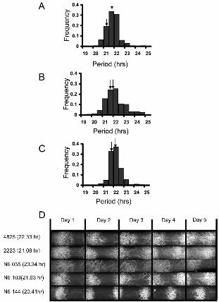
Figure 1. The circadian period variation in F1 populations. Phenotypic distributions of F1

progenies of N2 (A), N4 (B), and N6 (C) populations. X-axis represents circadian period and y-

axis represents frequency of period in the corresponding F1 progenies. Arrows indicate the

periods of the parents for each cross. (D) Race tube images of conidial banding patterns under

constant darkness (free running condition). The panel shows two N6 parents (FGSC 4825 and

FGSC 2223) and three representative progeny (N6 055, N6 103 and N6 144) with different free

running periods. The vertical black lines represent the growing front in 24 hr period. The number

in the parenthesis is the average period of the strain.

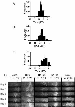
Figure 2. The entrained phase variation under 12:12 light/dark condition in F1 populations. The

phenotypic distribution of F1 progeny of N2 (A), N4 (B) and N6 (C) populations. X-axis

represents the entrained phase in ZT (see Materials and Methods) and y-axis represents

frequency of the periods of the corresponding F1 progeny. ZT 24 is the same as ZT 0. ZT 0 is

when light is on (dawn) and ZT 12 is when light is off (dusk). Arrows indicate the phases of the

parents for each cross. (D). Race tube images of conidial banding pattern under 12:12 LD cycles

for 5 days. The panel shows N6 parents (FGSC 4825 and FGSC 2223) and three representative

progeny (N6 163, N6 113 and N6 041) with different phases. The number in the parenthesis is

the average phase of the strain for 5 days. The arrow indicates the average phase value of each

strain.

23

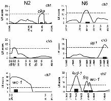
Figure 3. The graphical description of composite interval mapping (CIM) analysis in period

length under free running condition in N4 (A) and N6 (B) populations. X-axis of each panel

represents marker position within the linkage map. Y-axis of each panel represents likelihood

ratio (LR) score of each genetic position denoted by cM. Dotted line in each panel stands for

threshold level determined by 1000 permutation test. QTL names (indicated by arrows with

dotted line) and candidate genes in the corresponding QTL are shown around the peak position

of the QTL (refer to Table 3).

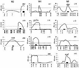
Figure 4. Graphical description of composite interval mapping (CIM) analysis in the phase under

the 12:12 LD cycle in N2(A), N4 (B) and N6 (C) population. X-axis of each panel represents

marker position within the linkage map. Y-axis of each panel represents likelihood ratio (LR)

score of each genetic position. Dotted line in each panel stands for threshold level determined by

1000 permutations. QTL names (indicated by arrows with dotted line) and candidate genes in the

corresponding QTL are shown around the peak position of the QTL (refer to Table 3).

Figure 5. Summary of Bayesian QTL analysis (BMQ). The distribution of PPT from BMQ

analysis for period and phase (A). Comparison of number of QTL using CIM (open bar) and

BMQ methods (filled bar). (B). Graphical description of CIM (square line) and BMQ (tri-angle

line) analysis. The x-axis represents the marker position in the linkage map. The primary y-axis

on the left is LR score for CIM analysis and secondary y-axis is PPT score for the BMQ

approach. (C). The average PPT (y-axis) in between QTL mapped by BMQ and CIM

simultaneously and QTL mapped by BMQ specifically (x-axis). Error bars represent standard

error around the mean. (D) Scatter plot analysis between LR score by CIM and by BMQ for each

24

QTL locus. In the panel (D), the variable plotted on the x-axis represents PPT of a QTL detected

by BMQ analysis and the y-axis is the LR score of the corresponding locus measured by CIM.

The diamond shaped dots with pink color are scatter plots representing QTL loci that are

commonly detected by BMQ and CIM. The QTL that are detected by BMQ specifically are

denoted by the rectangular shaped dots with blue color.

25

Legends for supplemental data.

Supplemental data Figure 1. Scatter plot analysis between period and phase in the N2, N4 and

N6 populations.

Supplemental data Figure 2. Distributions of PPT for neutral markers. A simulation with no

QTL (additive effects of 0) and four simulations with three QTL distributed uniformly

throughout the genome with additive effects 0.25, 0.5, 0.75, and 1 (heritabilities 0.13, 0.38, 0.58,

and 0.72 respectively) are shown. The distributions of PPT values for markers unlinked to QTL

across the genome (neutral markers) are represented as box plots. The middle line in each box

plot is the median, the boxes span the interquartile range, and the whiskers span the maximum

and minimum observations, unless there are outliers, which are defined as observations greater

than 1.5 times the interquartile range above or below the box. Outliers are represented as

pluses. The PPT value 0.17 (dotted line) was used as the threshold to eliminate false positives.

Supplemental data Figure 3. PPT for three simulated QTL. Three QTL were simulated with

additive effect 0.5 (heritability 0.38). The markers, 12, 36 and 60, were the true QTL (black

arrows). The simulation showed that the same markers have the highest PPT values. Although

the peak PPT occurs at the marker linked to the QTL, there was one neutral marker with a PPT

value higher than 0.17 (arrow head). The dotted line represents the threshold PPT, 0.17.

26

Supplemental data Figure 4. Distribution of PPTs of QTL in BMQ analysis. x-axis is range of

PPT and y-axis is frequency of a given PPT.

Supplemental data Figure 5. Comparison of average number of QTL detected for period and

phase phenotypes.

Supplemental data Figure 6. Venn diagram analysis of period (A) and phase QTL (B) among

populations.

Supplemental data Figure 7. Venn diagram analysis of between period and phase in population

specific (A and B) and all three populations (C).

Supplemental data Figure 8. Description of genetic relationship of mapping parents used in our

study. (A) Unrooted tree dendrogram based on dissimilarity clustering showing genetic

relationship of mapping parents of our study. (B) Randomly chosen SSR marker across N. crassa

genome that are used in (A). The primary axis (left) represents the frequency of the marker on a

chromosome. The secondary axis (right) represents length of chromosome.

27

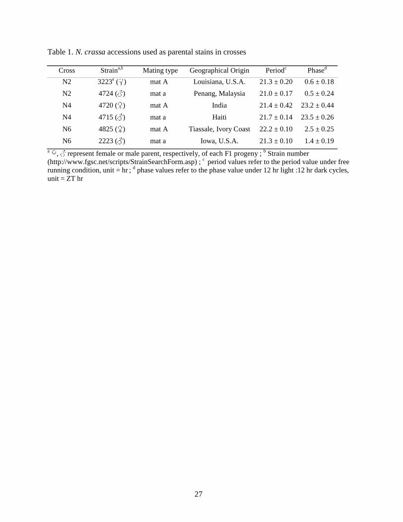
Table 1. N. crassa accessions used as parental stains in crosses

Cross Straina,b Mating type Geographical Origin Periodc Phased

N2 3223e (♀) mat A Louisiana, U.S.A. 21.3 ± 0.20 0.6 ± 0.18

N2 4724 (♂) mat a Penang, Malaysia 21.0 ± 0.17 0.5 ± 0.24

N4 4720 (♀) mat A India 21.4 ± 0.42 23.2 ± 0.44

N4 4715 (♂) mat a Haiti 21.7 ± 0.14 23.5 ± 0.26

N6 4825 (♀) mat A Tiassale, Ivory Coast 22.2 ± 0.10 2.5 ± 0.25

N6 2223 (♂) mat a Iowa, U.S.A. 21.3 ± 0.10 1.4 ± 0.19 a ♀, ♂ represent female or male parent, respectively, of each F1 progeny ; b Strain number (http://www.fgsc.net/scripts/StrainSearchForm.asp) ; c period values refer to the period value under free running condition, unit = hr ; d phase values refer to the phase value under 12 hr light :12 hr dark cycles, unit = ZT hr

28

Table 2. Phenotypic variation in period length and phase in N2, N4, and N6 populations

Percentage of progenies that show

transgressive segregation Phenotype Cross Meana STDEV Rangeb Heritabilityc

Total

(%)

(-) sided

(%)

(+) sidee

(%)

N2 21.4 0.62 4.60 0.62 47 31 69

Period N4 21.7 0.98 5.80 0.87 43 46 54

N6 21.7 0.57 4.10 0.85 20 54 46

N2 0.5 0.75 4.67 0.84 54 49 51

Phase N4 0.5 0.92 6.11 0.87 80 7 93

N6 1.9 1.05 4.14 0.74 44 49 51

a The unit for period is hr and for phase is ZT hr; b Range for period = highest phenotype - lowest phenotype; c Variance associated with the genotype effect by 2-way ANOVA and its significance, *p <0.05; ***p <0.001; d (-) side , percentage of progeny that show transgressive phenotypic segregation of lower phenotypic value than mean value of parental phenotypes in each mapping population; e (+) side , percentage of progeny that show transgressive phenotypic segregation of higher phenotypic value than mean value of parental phenotypes in each mapping population.

29

Table 3. Summary of the additive QTL in circadian properties that are segregated in three

different population formed by N. crassa natural accessions using Bayesian QTL analysis.

Cross Trait QTL ID Marker Chr a PPTb LRc

Additive

genetic

varianced

Origin of

allelic

effecte

Candidate

Genef (ncug)

N2 Phase N2BPha2-1 MN125 2 0.30 7.10 0.31 3223 na

N2 Phase N2CBPha2 MN229 2 0.72 25.30 0.46 4724 na

N2 Phase N2BPha3 MN173 3 0.19 5.50 0.25 3223 na

N2 Phase N2BPha4 MN182 4 0.17 5.90 0.26 3223 pp2a

(ncu06630.2)

N2 Phase N2CBPha5-1 MN051 5 0.78 31.50 0.48 4724 na

N2 Phase N2CBPha6 MN054 6 0.46 14.70 0.36 3223 vvd

(ncu03967.2)


N4 Period N4CBPer1-1 MN008 1 0.16 4.8 0.28 4715 na

N4 Period N4CBPer1-3 MN129 1 0.19 4.3 0.29 4715 prd-4

(ncu02814.2)

N4 Period N4CBPer1-2 MN042 1 0.30 12 0.41 4720 ckII catalytic

subunit (ncu03124.2))

N4 Period N4BPer2 MN094 2 0.44 9.4 0.38 4715 na



N4 Period N4CBPer5 MN153 5 0.58 11.3 0.45 4720 na

N4 Period N4CBPer7 MN046 7 0.95 32.1 0.66 4720 wc-1

(ncu02356.2)

N4 Phase N4CBPha1-1 MN008 1 0.42 15.5 0.35 4715 na


N4 Phase N4BPha1-2 MN129 1 0.22 3 0.26 4715 prd-4

(ncu02814.2)


N4 Phase N4CBPha4-2 MN090 4 0.57 16.3 0.39 4715 pp2a

(ncu06630.2)





N6 Period N6BPer4-1 MN075 4 0.20 0.6 0.22 4825 na

30



N6 Period N6CPer-7-3 MN046 7 0.00 15.2 na 2223 wc-1

(ncu02356.2)

N6 Period N6CPer-7-2 MN046 7 0.10 17.75 na 2223 frq

(ncu02265.2)

N6 Period N6CBPer-7-1 MN168 7 0.95 29.6 0.35 4825 fwd-1

(ncu045450.2) N6 Phase N6BPha1-1 MN018 1 0.56 5.4 0.39 2223 na

N6 Phase N6CBPha1-2 MN131 1 0.79 10.2 0.37 4825 prd-4

(ncu02814.2)

N6 Phase N6CBPha1-3 MN041 1 0.55 21.5 0.38 2223 ckII catalytic

subunit (ncu03124.2)







N6 Phase N6BPha5 MN155 5 0.36 4.4 0.49 4825 na


N6 Phase N6CBPha6 MN054 6 0.96 21.9 0.79 4825 vvd

(ncu03967.2)

N6 Phase N6CBPha6-1 MN067 6 0.69 10.4 0.41 2223 na a chr., chromosome number; b PPT, Posterior Probability; c LR, Likelihood ratio; d, In this column, the estimation of additive genetic variance value originates from Bayesian multiple QTL analysis. e, Each number in this column represents the accession number used in Fungal Genetics Stock Center (www.fgsc.net); f The range of each candidate gene is plus and minus 200-300 kilobase pair (kbp) at the genetic locus where LR score or PPT is maximized. In this column, na = not available, which means no previously characterized clock gene is available; g For cases in which a candidate gene is available, the corresponding NCU number is recorded in parentheses (Broad Institute, http://www.broad.mit.edu/annotation/genome/neurospora/Home.html).

31

LITERATURE CITED

ABIOLA, O., J. M. ANGEL, P. AVNER, A. A. BACHMANOV, J. K. BELKNAP et al., 2003 The nature

and identification of quantitative trait loci: a community's view. Nat Rev Genet 4: 911-

916.

ALONSO-BLANCO, C., and M. KOORNNEEF, 2000 Naturally occurring variation in Arabidopsis:

an underexploited resource for plant genetics. Trends Plant Sci 5: 22-29.

ARONSON, B. D., K. A. JOHNSON and J. C. DUNLAP, 1994 Circadian clock locus frequency:

protein encoded by a single open reading frame defines period length and temperature

compensation. Proc Natl Acad Sci U S A 91: 7683-7687.

BASTEN, C. J., B. S. WEIR and Z.-B. ZENG, 2006 Windows QTL Cartographer 2.5. Department

of Statistics, North Carolina State University, Raleigh, NC.

(http://statgen.ncsu.edu/qtlcart/WQTLCart.htm).

BELDEN, W. J., L. F. LARRONDO, A. C. FROEHLICH, M. SHI, C. H. CHEN et al., 2007 The band

mutation in Neurospora crassa is a dominant allele of ras-1 implicating RAS signaling in

circadian output. Genes Dev 21: 1494-1505.

BELL-PEDERSEN, D., V. M. CASSONE, D. J. EARNEST, S. S. GOLDEN, P. E. HARDIN et al., 2005

Circadian rhythms from multiple oscillators: lessons from diverse organisms. Nat Rev

Genet 6: 544-556.

BELL-PEDERSEN, D., S. K. CROSTHWAITE, P. L. LAKIN-THOMAS, M. MERROW and M. OKLAND,

2001 The Neurospora circadian clock: simple or complex? Philos Trans R Soc Lond B

Biol Sci 356: 1697-1709.

32

CHO, Y. G., T. ISHII, S. TEMNYKH, X. CHEN, L. LIPOVICH et al., 2000 Diversity of microsatellites

derived from genomic libraries and GenBank sequences in rice (Oryza sativa L.). Theor

Appl Genet 100: 713-722.

CHURCHILL, G. A., and R. W. DOERGE, 1994 Empirical threshold values for quantitative trait

mapping. Genetics 138: 963-971.

DARRAH, C., B. L. TAYLOR, K. D. EDWARDS, P. E. BROWN, A. HALL et al., 2006 Analysis of

phase of LUCIFERASE expression reveals novel circadian quantitative trait loci in

Arabidopsis. Plant Physiol 140: 1464-1474.

DAVIS, R. H., 2000 Neurospora, contributions of a model organism. Oxford University Press,

Inc., New York.

DAVIS, R. H., and D. D. PERKINS, 2002 Timeline: Neurospora: a model of model microbes. Nat

Rev Genet 3: 397-403.

DOERGE, R. W., 2002 Mapping and analysis of quantitative trait loci in experimental populations.

Nat Rev Genet 3: 43-52.

DUNLAP, J. C., and J. J. LOROS, 2004 The Neurospora circadian system. J Biol Rhythms 19: 414-

424.

DUNLAP, J. C., and J. J. LOROS, 2006 How fungi keep time: circadian system in Neurospora and

other fungi. Curr Opin Microbiol 9: 579-587.

EDWARDS, K. D., P. E. ANDERSON, A. HALL, N. S. SALATHIA, J. C. LOCKE et al., 2006

FLOWERING LOCUS C mediates natural variation in the high-temperature response of

the Arabidopsis circadian clock. Plant Cell 18: 639-650.

33

EDWARDS, K. D., J. R. LYNN, P. GYULA, F. NAGY and A. J. MILLAR, 2005 Natural allelic

variation in the temperature-compensation mechanisms of the Arabidopsis thaliana

circadian clock. Genetics 170: 387-400.

ELVIN, M., J. J. LOROS, J. C. DUNLAP and C. HEINTZEN, 2005 The PAS/LOV protein VIVID

supports a rapidly dampened daytime oscillator that facilitates entrainment of the

Neurospora circadian clock. Genes Dev 19: 2593-2605.

FELDMAN, J. F., and M. N. HOYLE, 1973 Isolation of circadian clock mutants of Neurospora

crassa. Genetics 75: 605-613.

GALAGAN, J. E., S. E. CALVO, K. A. BORKOVICH, E. U. SELKER, N. D. READ et al., 2003 The

genome sequence of the filamentous fungus Neurospora crassa. Nature 422: 859-868.

GEORGE, E. I., and R. E. MCCULLOCH, 1993 Variable selection via Gibbs sampling. Amer.

Statist. Assoc. 88: 881-889.

HACKETT, C. A., and L. B. BROADFOOT, 2003 Effects of genotyping errors, missing values and

segregation distortion in molecular marker data on the construction of linkage maps.

Heredity 90: 33-38.

HE, Q., H. SHU, P. CHENG, S. CHEN, L. WANG et al., 2005 Light-independent phosphorylation of

WHITE COLLAR-1 regulates its function in the Neurospora circadian negative feedback

loop. J Biol Chem 280: 17526-17532.

HEINTZEN, C., J. J. LOROS and J. C. DUNLAP, 2001 The PAS protein VIVID defines a clock-

associated feedback loop that represses light input, modulates gating, and regulates clock

resetting. Cell 104: 453-464.

34

HOFSTETTER, J. R., A. R. MAYEDA, B. POSSIDENTE and J. I. NURNBERGER, JR., 1995

Quantitative trait loci (QTL) for circadian rhythms of locomotor activity in mice. Behav

Genet 25: 545-556.

HOFSTETTER, J. R., B. POSSIDENTE and A. R. MAYEDA, 1999 Provisional QTL for circadian

period of wheel running in laboratory mice: quantitative genetics of period in RI mice.

Chronobiol Int 16: 269-279.

JORDAN, K. W., T. J. MORGAN and T. F. MACKAY, 2006 Quantitative trait loci for locomotor

behavior in Drosophila melanogaster. Genetics 174: 271-284.

KAO, C. H., Z. B. ZENG and R. D. TEASDALE, 1999 Multiple interval mapping for quantitative

trait loci. Genetics 152: 1203-1216.

KERNEK, K. L., J. A. TROFATTER, A. R. MAYEDA and J. R. HOFSTETTER, 2004 A locus for

circadian period of locomotor activity on mouse proximal chromosome 3. Chronobiol Int

21: 343-352.

KIM, T., J. BOOTH, H. G. GAUCH, Q. SUN, J. PARK et al., 2007 Simple Sequence Repeats in

Neurospora crassa: distribution, polymorphism and evolutionary inference. BMC

genomics in press.

KOPP, C., 2001 Locomotor activity rhythm in inbred strains of mice: implications for behavioral

studies. Behav Brain Res 125: 93-96.

LAKIN-THOMAS, P. L., 2006 Transcriptional feedback oscillators: maybe, maybe not. J Biol

Rhythms 21: 83-92.

LANDER, E. S., and N. J. SCHORK, 1994 Genetic dissection of complex traits. Science 265: 2037-

2048.

35

LEE, K., J. C. DUNLAP and J. J. LOROS, 2003 Roles for WHITE COLLAR-1 in circadian and

general photoperception in Neurospora crassa. Genetics 163: 103-114.

LEIPS, J., P. GILLIGAN and T. F. MACKAY, 2006 Quantitative trait loci with age-specific effects

on fecundity in Drosophila melanogaster. Genetics 172: 1595-1605.

LIAO, J. G., 1999 A hierarchical Bayesian model for combining multiple 2 x 2 tables using

conditional likelihoods. Biometrics 55: 268-272.

LIU, Y., and D. BELL-PEDERSEN, 2006 Circadian rhythms in Neurospora crassa and other

filamentous fungi. Eukaryot Cell 5: 1184-1193.

LOROS, J. J., and J. C. DUNLAP, 2001 Genetic and molecular analysis of circadian rhythms in

Neurospora. Annu Rev Physiol 63: 757-794.

MACKAY, T. F., 2001a The genetic architecture of quantitative traits. Annu Rev Genet 35: 303-

339.

MACKAY, T. F., 2001b Quantitative trait loci in Drosophila. Nat Rev Genet 2: 11-20.

MAYEDA, A. R., and J. R. HOFSTETTER, 1999 A QTL for the genetic variance in free-running

period and level of locomotor activity between inbred strains of mice. Behav Genet 29:

171-176.

MICHAEL, T. P., S. PARK, T. S. KIM, J. BOOTH, A. BYER et al., 2007 Simple Sequence Repeats

Provide a Substrate for Phenotypic Variation in the Neurospora crassa Circadian Clock.

PLoS ONE 2: e795.

MICHAEL, T. P., P. A. SALOME, H. J. YU, T. R. SPENCER, E. L. SHARP et al., 2003 Enhanced

fitness conferred by naturally occurring variation in the circadian clock. Science 302:

1049-1053.

36

OKAMURA, H., 2004 Clock genes in cell clocks: roles, actions, and mysteries. J Biol Rhythms

19: 388-399.

PARK, S., and K. LEE, 2004 Inverted race tube assay for circadian clock studies of the

Neurospora accessions. Fungal Genet. Newsl. 51: 12-14.

PLAUTZ, J. D., M. STRAUME, R. STANEWSKY, C. F. JAMISON, C. BRANDES et al., 1997

Quantitative analysis of Drosophila period gene transcription in living animals. J Biol

Rhythms 12: 204-217.

PREGUEIRO, A. M., Q. LIU, C. L. BAKER, J. C. DUNLAP and J. J. LOROS, 2006 The Neurospora

checkpoint kinase 2: a regulatory link between the circadian and cell cycles. Science 313:

644-649.

SALATHIA, N., K. EDWARDS and A. J. MILLAR, 2002 QTL for timing: a natural diversity of clock

genes. Trends Genet 18: 115-118.

SARGENT, M. L., and S. H. KALTENBORN, 1972 Effects of Medium Composition and Carbon

Dioxide on Circadian Conidiation in Neurospora. Plant Physiol 50: 171-175.

SARGENT, M. L., and D. O. WOODWARD, 1969 Genetic determinants of circadian rhythmicity in

Neurospora. J Bacteriol 97: 861-866.

SCHIBLER, U., 2006 Circadian time keeping: the daily ups and downs of genes, cells, and

organisms. Prog Brain Res 153: 271-282.

SCHUELKE, M., 2000 An economic method for the fluorescent labeling of PCR fragments. Nat

Biotechnol 18: 233-234.

SHIMOMURA, K., S. S. LOW-ZEDDIES, D. P. KING, T. D. STEEVES, A. WHITELEY et al., 2001

Genome-wide epistatic interaction analysis reveals complex genetic determinants of

circadian behavior in mice. Genome Res 11: 959-980.

37

STANEWSKY, R., 2003 Genetic analysis of the circadian system in Drosophila melanogaster and

mammals. J Neurobiol 54: 111-147.

SUZUKI, T., A. ISHIKAWA, T. YOSHIMURA, T. NAMIKAWA, H. ABE et al., 2001 Quantitative trait

locus analysis of abnormal circadian period in CS mice. Mamm Genome 12: 272-277.

SWARUP, K., C. ALONSO-BLANCO, J. R. LYNN, S. D. MICHAELS, R. M. AMASINO et al., 1999

Natural allelic variation identifies new genes in the Arabidopsis circadian system. Plant J

20: 67-77.

TER BRAAK, C. J., M. P. BOER and M. C. BINK, 2005 Extending Xu's Bayesian model for

estimating polygenic effects using markers of the entire genome. Genetics 170: 1435-

1438.

TOTH, L. A., and R. W. WILLIAMS, 1999 A quantitative genetic analysis of locomotor activity in

CXB recombinant inbred mice. Behav Genet 29: 319-328.

WELCH, S. M., Z. S. DONG, J. L. ROE and S. DAS, 2005 Flowering time control: gene network

modelling and the link to quantitative genetics. Australian Journal of Agricultural

Research 56: 919-936.

XIE, C. Q., D. D. G. GESSLER and S. Z. XU, 1998 Combining different line crosses for mapping

quantitative trait loci using the identical by descent-based variance component method.

Genetics 149: 1139-1146.

YI, N., S. XU and D. B. ALLISON, 2003 Bayesian model choice and search strategies for mapping

interacting quantitative trait Loci. Genetics 165: 867-883.

YOUNG, M. W., and S. A. KAY, 2001 Time zones: a comparative genetics of circadian clocks.

Nat Rev Genet 2: 702-715.

38

YU, J.-K., R. V. KANTETY, E. GRAZNAK, D. BENSCHER, H. TEFERA et al., 2006 A genetic

linkage map for tef [Eragrostis tef (Zucc.) Trotter]. Theor Appl Genet 113: 1093-1102.

ZENG, Z. B., 1993 Theoretical basis for separation of multiple linked gene effects in mapping

quantitative trait loci. Proc Natl Acad Sci U S A 90: 10972-10976.

ZENG, Z. B., 1994 Precision mapping of quantitative trait loci. Genetics 136: 1457-1468.

ZENG, Z. B., C. H. KAO and C. J. BASTEN, 1999 Estimating the genetic architecture of

quantitative traits. Genet Res 74: 279-289.

ZHANG, M., K. L. MONTOOTH, M. T. WELLS, A. G. CLARK and D. ZHANG, 2005 Mapping

multiple Quantitative Trait Loci by Bayesian classification. Genetics 169: 2305-2318.

Quantitative Trait Loci for the Circadian Clock in Neurospora crassa

Documents