Quantitative Methods – I - AY 2020-21 ____ Practice 1

Quantitative Methods – IA.Y. 2020-21

____Practice 1

Lorenzo Cavallo [email protected]

1

2

THEME #1

___

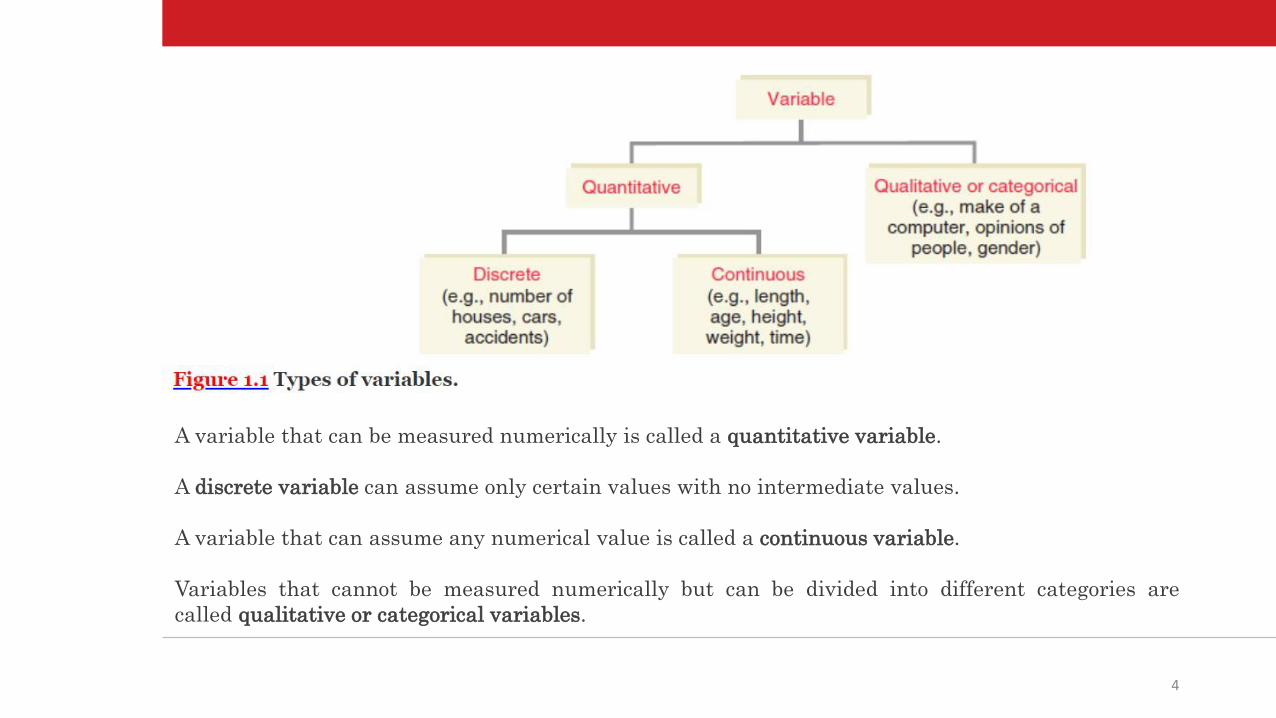
Types of Variables

3

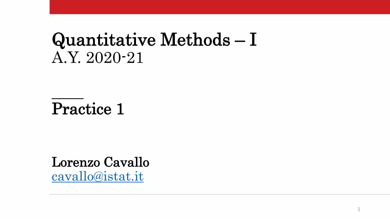
Element or member

Variable

Observation or measurement

Data set

a. Number of Billionaires by Country

b. n=413+115+101+55+52+32+30+26=824

c. 8 (United States, China, etc.)

4

A variable that can be measured numerically is called a quantitative variable.

A discrete variable can assume only certain values with no intermediate values.

A variable that can assume any numerical value is called a continuous variable.

Variables that cannot be measured numerically but can be divided into different categories are

called qualitative or categorical variables.

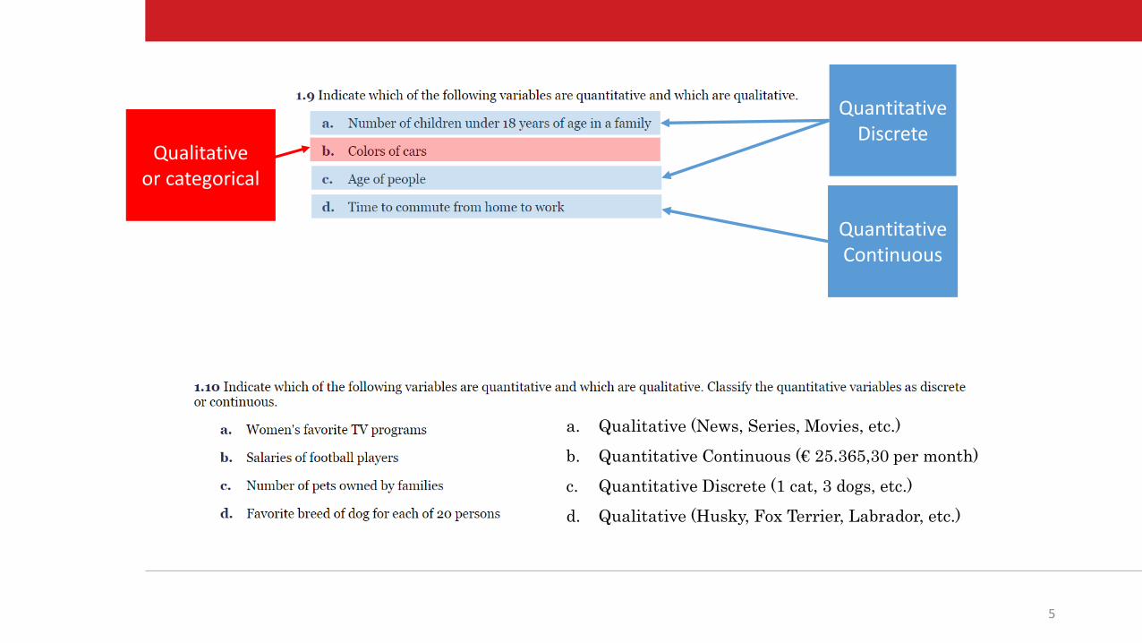
5

QuantitativeDiscrete

QuantitativeContinuous

Qualitativeor categorical

a. Qualitative (News, Series, Movies, etc.)

b. Quantitative Continuous (€ 25.365,30 per month)

c. Quantitative Discrete (1 cat, 3 dogs, etc.)

d. Qualitative (Husky, Fox Terrier, Labrador, etc.)

6

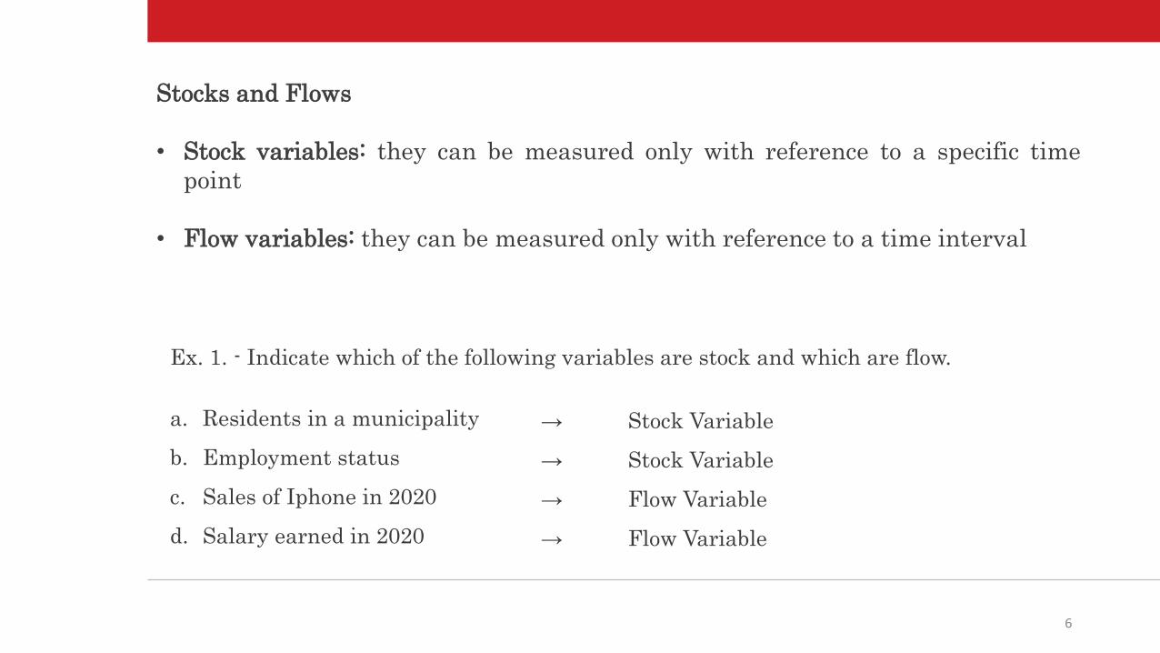
Stocks and Flows

• Stock variables: they can be measured only with reference to a specific time

point

• Flow variables: they can be measured only with reference to a time interval

Ex. 1. - Indicate which of the following variables are stock and which are flow.

a. Residents in a municipality

b. Employment status

c. Sales of Iphone in 2020

d. Salary earned in 2020

→ Stock Variable

→ Stock Variable

→ Flow Variable

→ Flow Variable

7

THEME #2

___

Organizing and Graphing Data

8

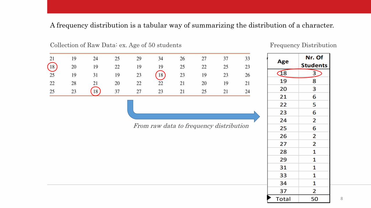
Collection of Raw Data: ex. Age of 50 students

From raw data to frequency distribution

Frequency Distribution

A frequency distribution is a tabular way of summarizing the distribution of a character.

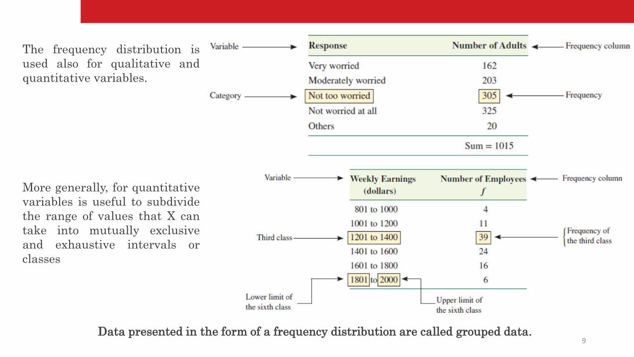
9Data presented in the form of a frequency distribution are called grouped data.

The frequency distribution is

used also for qualitative and

quantitative variables.

More generally, for quantitative

variables is useful to subdivide

the range of values that X can

take into mutually exclusive

and exhaustive intervals or

classes

10

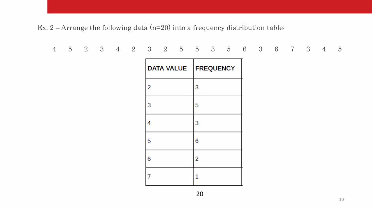
Ex. 2 – Arrange the following data (n=20) into a frequency distribution table:

4 5 2 3 4 2 3 2 5 5 3 5 6 3 6 7 3 4 5

20

11

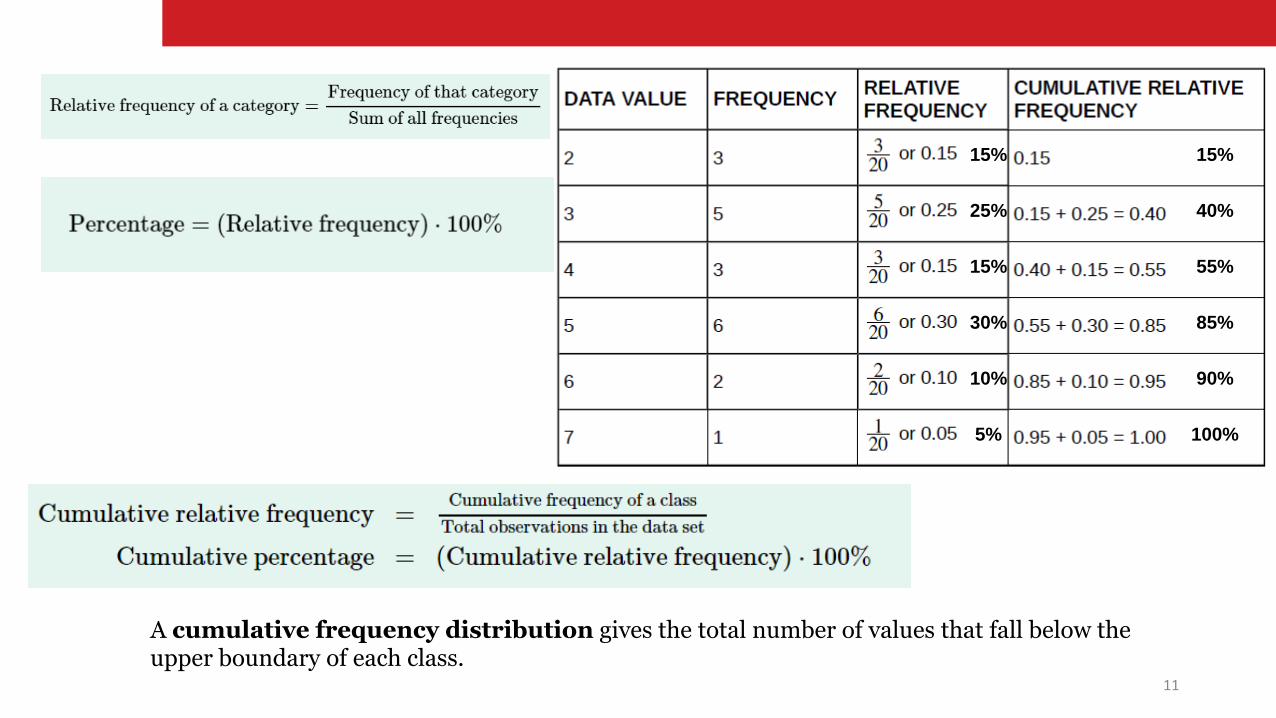
A cumulative frequency distribution gives the total number of values that fall below the upper boundary of each class.

15%

25%

15%

30%

10%

5%

15%

40%

55%

85%

90%

100%

12

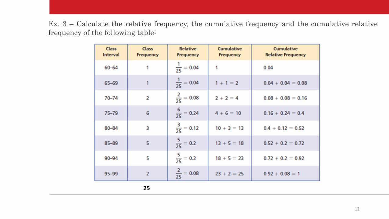
Ex. 3 – Calculate the relative frequency, the cumulative frequency and the cumulative relative

frequency of the following table:

25

13

14

THEME #4

___

Graphical representations of

frequency distributions

15

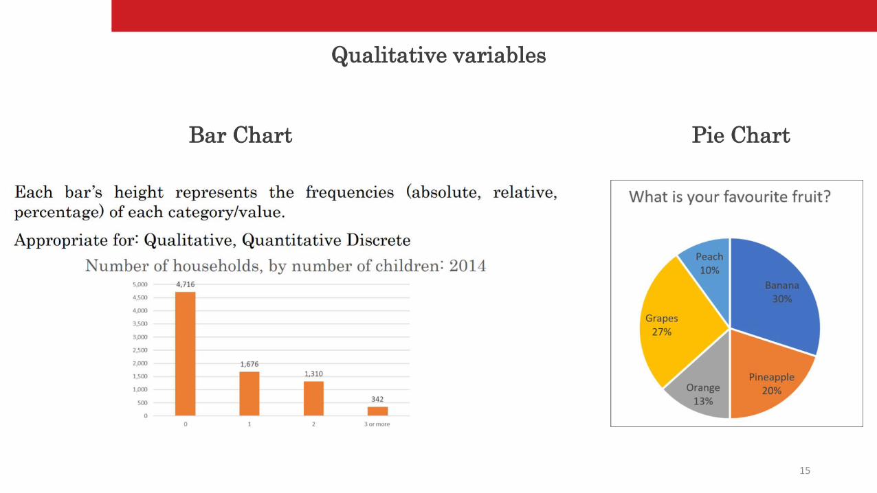
Bar Chart

Qualitative variables

Pie Chart

16

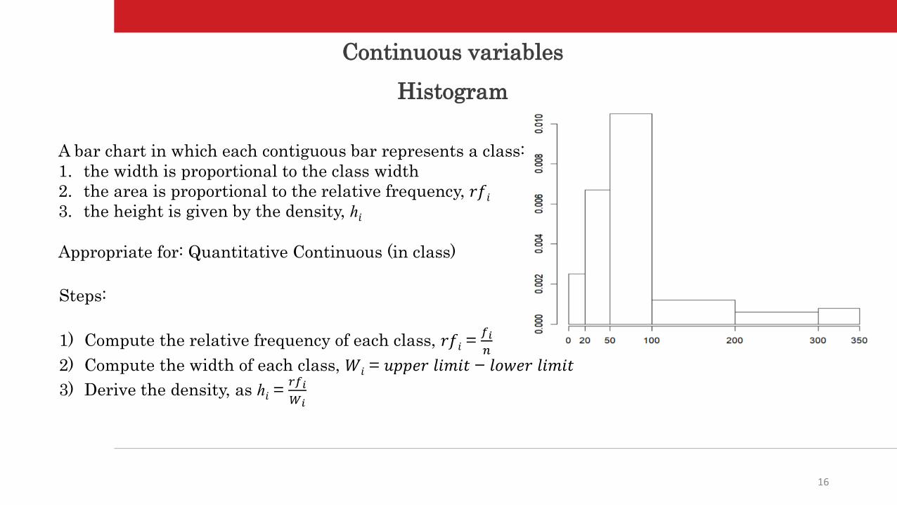
Continuous variables

Histogram

A bar chart in which each contiguous bar represents a class:

1. the width is proportional to the class width

2. the area is proportional to the relative frequency, 𝑟𝑓𝑖3. the height is given by the density, ℎ𝑖

Appropriate for: Quantitative Continuous (in class)

Steps:

1) Compute the relative frequency of each class, 𝑟𝑓𝑖 = 𝑓𝑖

𝑛

2) Compute the width of each class, 𝑊𝑖 = 𝑢𝑝𝑝𝑒𝑟 𝑙𝑖𝑚𝑖𝑡 − 𝑙𝑜𝑤𝑒𝑟 𝑙𝑖𝑚𝑖𝑡

3) Derive the density, as ℎ𝑖 = 𝑟𝑓𝑖

𝑊𝑖

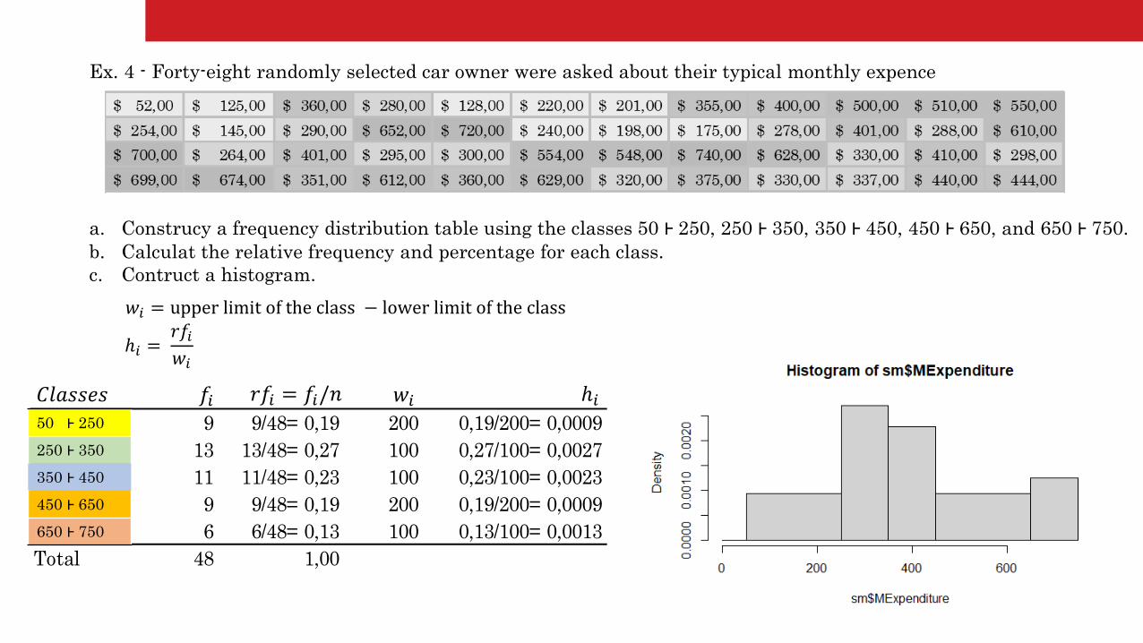
$ 52,00 $ 125,00 $ 360,00 $ 280,00 $ 128,00 $ 220,00 $ 201,00 $ 355,00 $ 400,00 $ 500,00 $ 510,00 $ 550,00

$ 254,00 $ 145,00 $ 290,00 $ 652,00 $ 720,00 $ 240,00 $ 198,00 $ 175,00 $ 278,00 $ 401,00 $ 288,00 $ 610,00

$ 700,00 $ 264,00 $ 401,00 $ 295,00 $ 300,00 $ 554,00 $ 548,00 $ 740,00 $ 628,00 $ 330,00 $ 410,00 $ 298,00

$ 699,00 $ 674,00 $ 351,00 $ 612,00 $ 360,00 $ 629,00 $ 320,00 $ 375,00 $ 330,00 $ 337,00 $ 440,00 $ 444,00

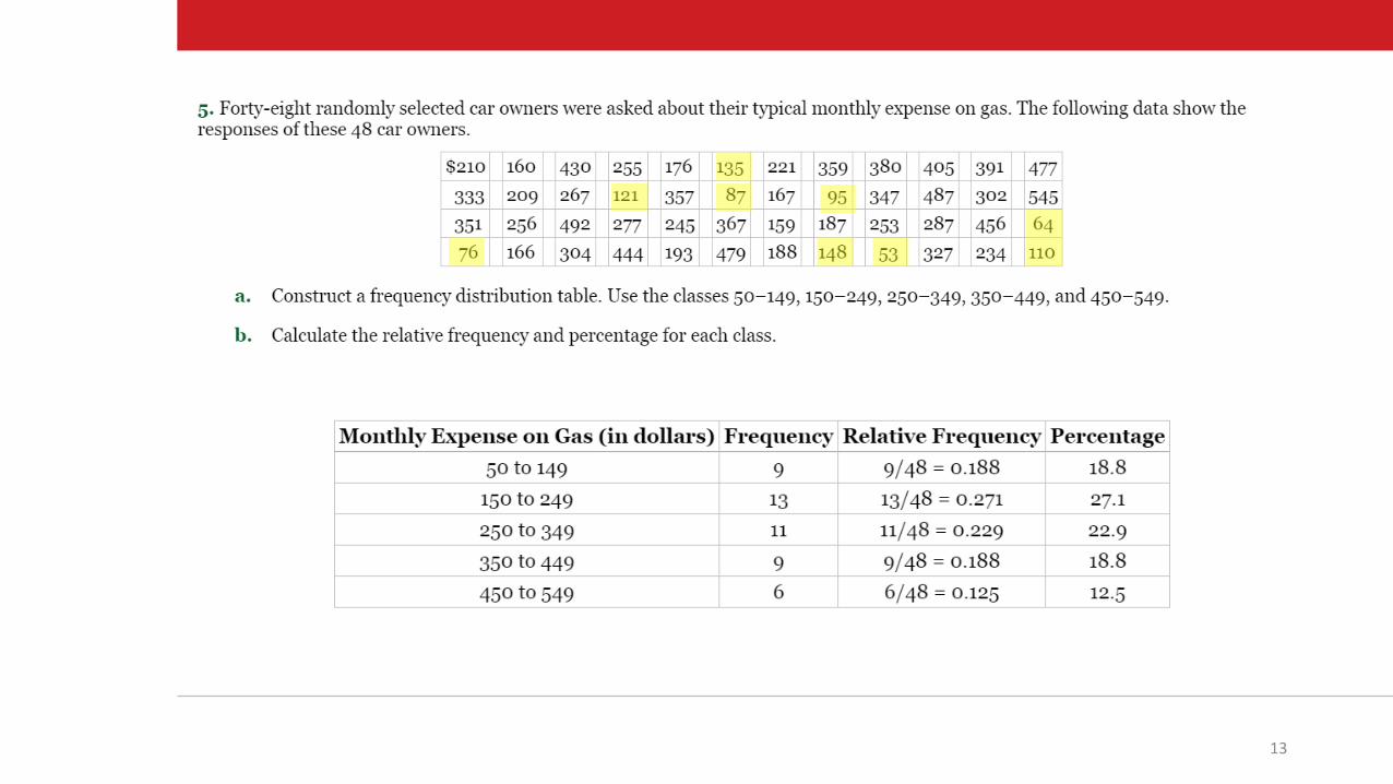
a. Construct a frequency distribution table. Use the classes 50–249, 250–349, 350–449, 450–649, and 650–749.

b. Calculate the relative frequency and percentage for each class.

c. Construct a histogram.

Classes fi rfi wi hi

50 to 249 9 0,19 200 0,0009

250 to 349 13 0,27 100 0,0027

350 to 449 11 0,23 100 0,0023

450 to 649 9 0,19 200 0,0009

650 to 749 6 0,13 100 0,0013

Total 48 1

Forty-eight randomly selected car owners were asked about their typical monthly expense

17

ℎ𝑖 =𝑟𝑓𝑖𝑤𝑖

𝑤𝑖 = upper limit of the class − lower limit of the class

Classes fi rfi wi hi

50 to 249 9 9/48= 0,19 200 0,19/200= 0,0009

250 to 349 13 13/48= 0,27 100 0,27/100= 0,0027

350 to 449 11 11/48= 0,23 100 0,23/100= 0,0023

450 to 649 9 9/48= 0,19 200 0,19/200= 0,0009

650 to 749 6 6/48= 0,13 100 0,13/100= 0,0013

Total 48 1,00

𝑤𝑖 ℎ𝑖𝑟𝑓𝑖 = 𝑓𝑖/𝑛𝐶𝑙𝑎𝑠𝑠𝑒𝑠 𝑓𝑖

Ex. 4 - Forty-eight randomly selected car owner were asked about their typical monthly expence

a. Construcy a frequency distribution table using the classes 50 Ⱶ 250, 250 Ⱶ 350, 350 Ⱶ 450, 450 Ⱶ 650, and 650 Ⱶ 750.

b. Calculat the relative frequency and percentage for each class.

c. Contruct a histogram.

50 Ⱶ 250

250 Ⱶ 350

350 Ⱶ 450

450 Ⱶ 650

650 Ⱶ 750

18

THEME #4

___

Measures of position

19

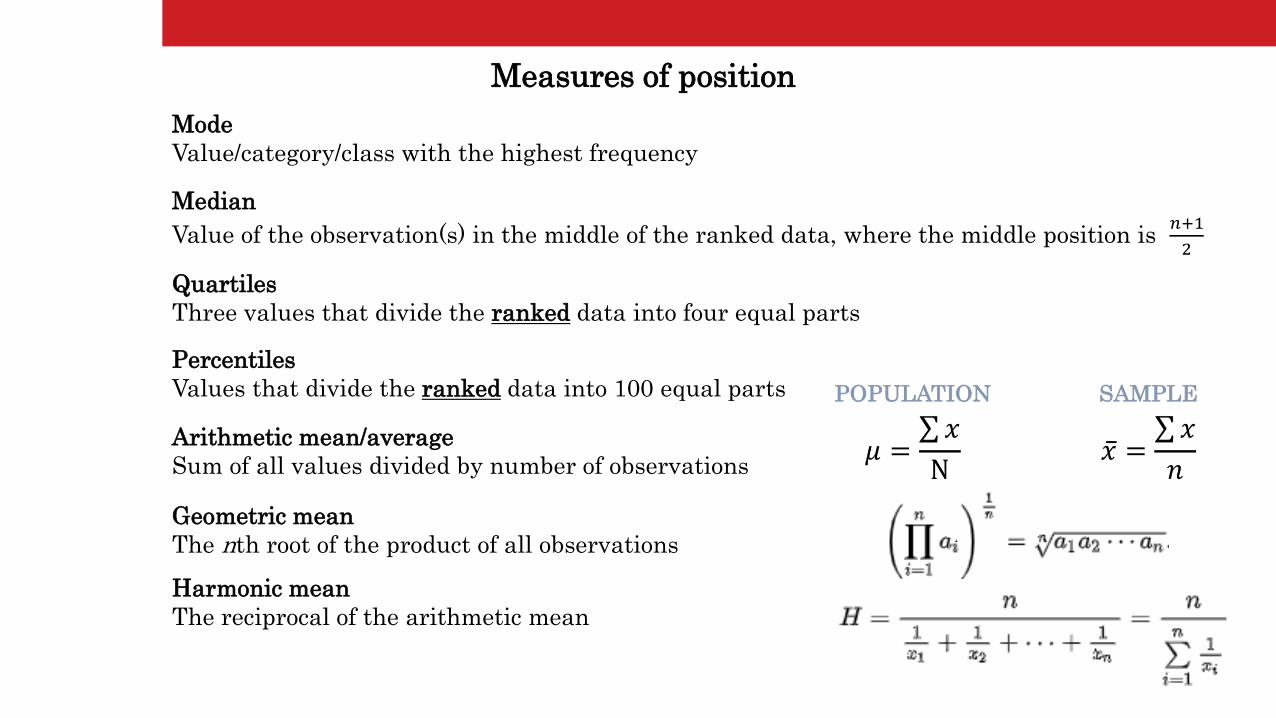
Mode

Value/category/class with the highest frequency

Median

Value of the observation(s) in the middle of the ranked data, where the middle position is 𝑛+1

2

Quartiles

Three values that divide the ranked data into four equal parts

Percentiles

Values that divide the ranked data into 100 equal parts

Arithmetic mean/average

Sum of all values divided by number of observations

Geometric mean

The nth root of the product of all observations

Harmonic mean

The reciprocal of the arithmetic mean

Measures of position

20

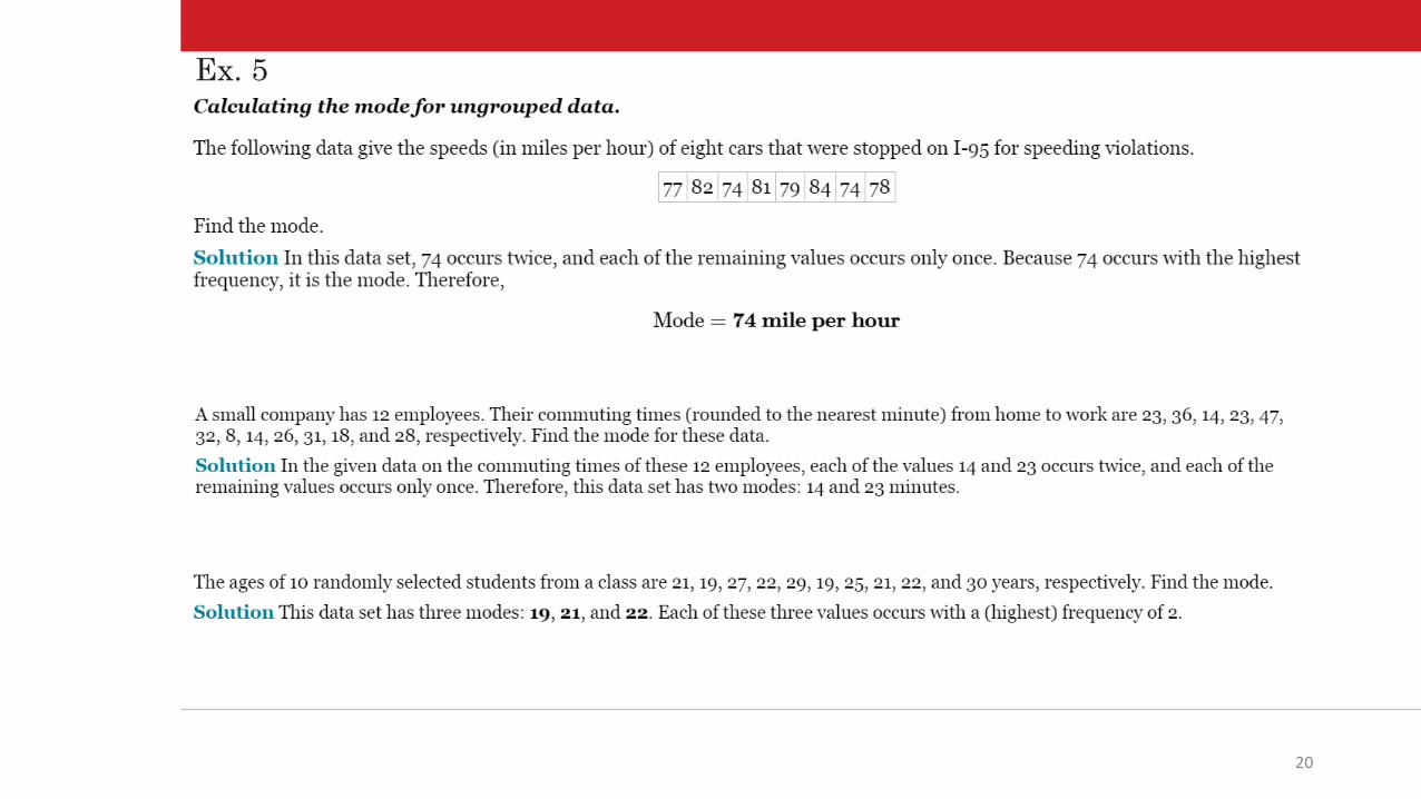
Ex. 5

21

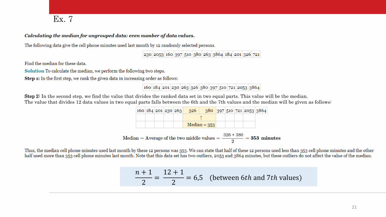
326 + 380

𝑛 + 1

2=

12 + 1

2= 6,5 (between 6𝑡ℎ and 7𝑡ℎ values)

Step 2: In the second step, we find the value that divides the ranked data set in two equal parts. This value will be the median.

The value that divides 12 data values in two equal parts falls between the 6th and the 7th values and the median will be given as follows:

Ex. 7

22

Ex. 8

23

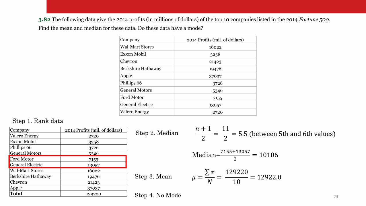
Company 2014 Profits (mil. of dollars)

Wal-Mart Stores 16022

Exxon Mobil 3258

Chevron 21423

Berkshire Hathaway 19476

Apple 37037

Phillips 66 3726

General Motors 5346

Ford Motor 7155

General Electric 13057

Valero Energy 2720

3.82 The following data give the 2014 profits (in millions of dollars) of the top 10 companies listed in the 2014 Fortune 500.

Find the mean and median for these data. Do these data have a mode?

Company 2014 Profits (mil. of dollars)

Valero Energy 2720

Exxon Mobil 3258

Phillips 66 3726

General Motors 5346

Ford Motor 7155

General Electric 13057

Wal-Mart Stores 16022

Berkshire Hathaway 19476

Chevron 21423

Apple 37037

Total 129220

𝜇 =σ𝑥

𝑁=

129220

10= 12922.0

Step 1. Rank data

Step 2. Median

Step 3. Mean

𝑛 + 1

2=

11

2= 5.5 (between 5th and 6th values)

Median=7155+13057

2= 10106

Step 4. No Mode

24

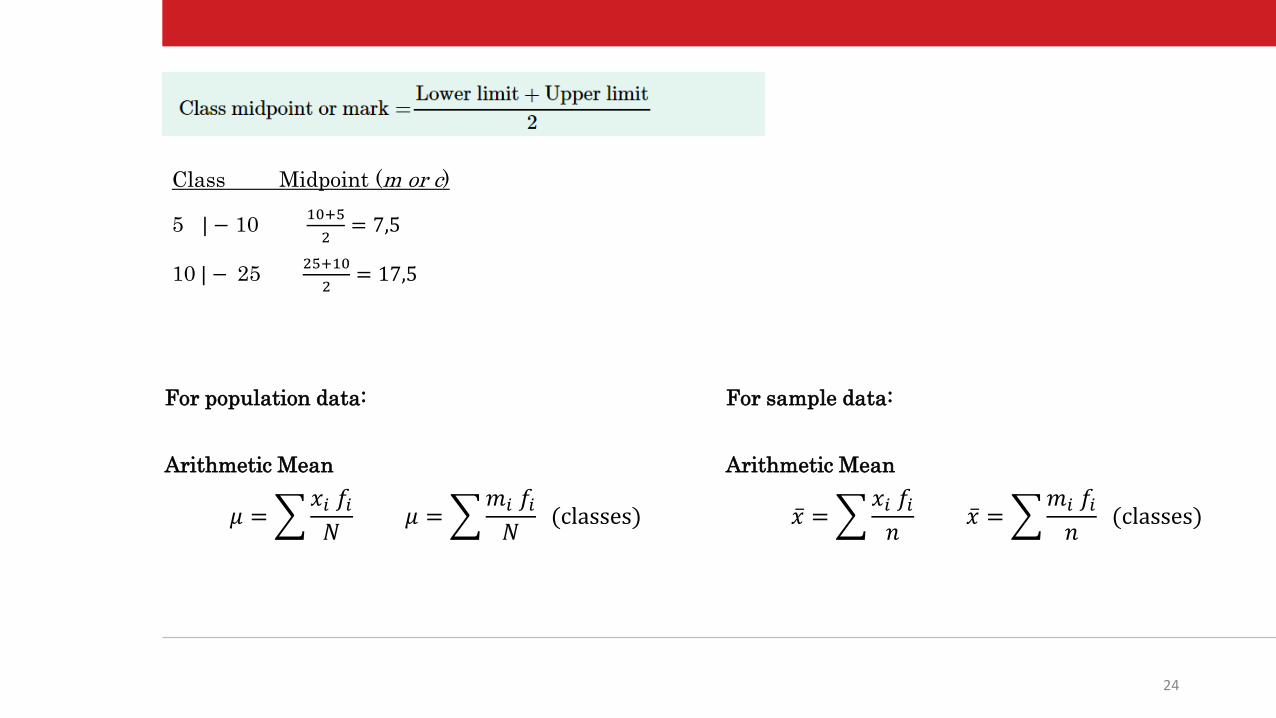
Class Midpoint (m or c)

5 | − 10 10+5

2= 7,5

10 | − 25 25+10

2= 17,5

For population data:

Arithmetic Mean

𝜇 =𝑥𝑖 𝑓𝑖𝑁

𝜇 =𝑚𝑖 𝑓𝑖𝑁

(classes)

For sample data:

Arithmetic Mean

ҧ𝑥 = 𝑥𝑖 𝑓𝑖𝑛

ҧ𝑥 = 𝑚𝑖 𝑓𝑖𝑛

(classes)

25

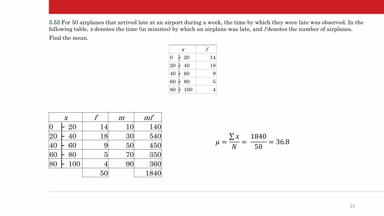
x f

0 ├ 20 14

20 ├ 40 18

40 ├ 60 9

60 ├ 80 5

80 ├ 100 4

3.53 For 50 airplanes that arrived late at an airport during a week, the time by which they were late was observed. In the

following table, x denotes the time (in minutes) by which an airplane was late, and f denotes the number of airplanes.

Find the mean.

x f m mf

0 ├ 20 14 10 140

20 ├ 40 18 30 540

40 ├ 60 9 50 450

60 ├ 80 5 70 350

80 ├ 100 4 90 360

50 1840

𝜇 =σ𝑥

𝑁=

1840

50= 36.8

26

THEME #5

___

Measures of dispersion

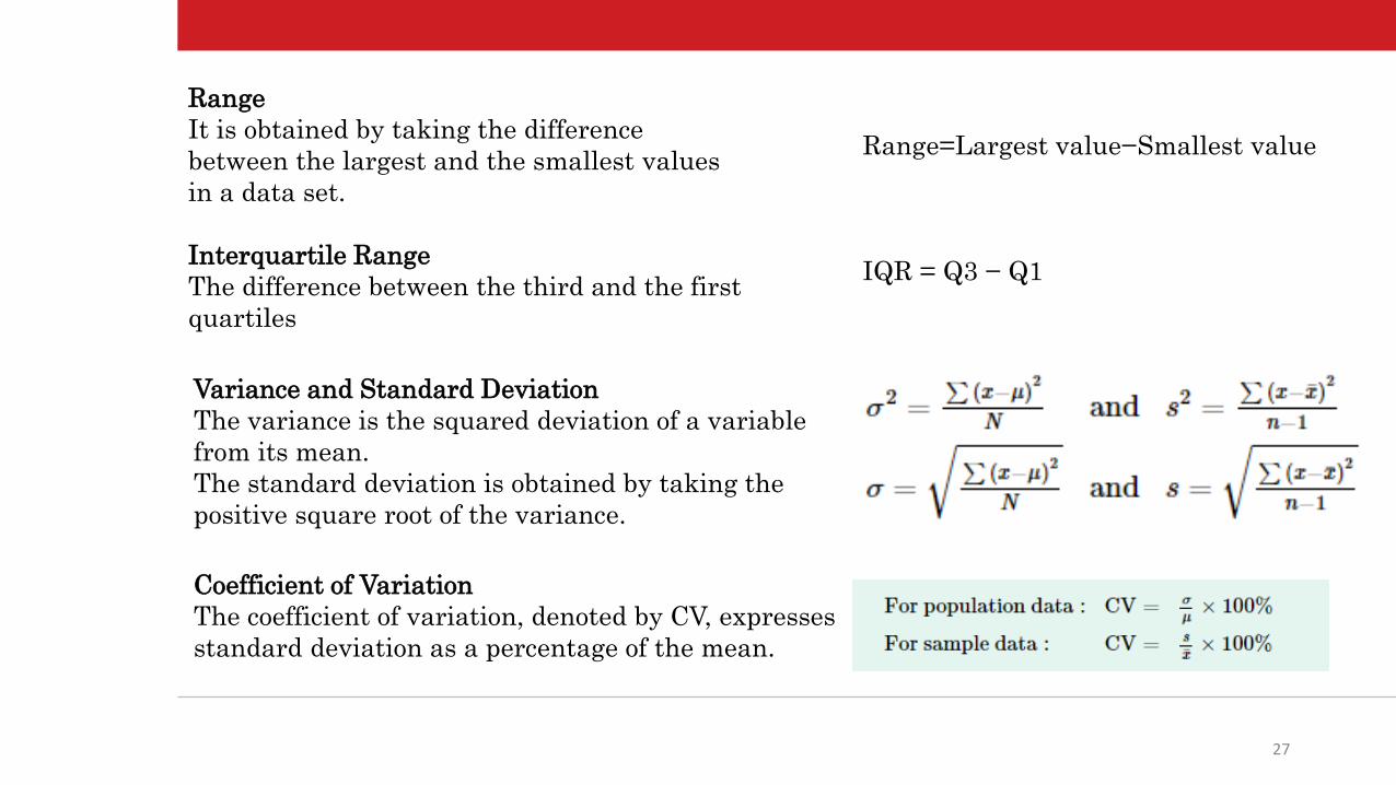
27

Range

It is obtained by taking the difference

between the largest and the smallest values

in a data set.

Interquartile Range

The difference between the third and the first

quartiles

Range=Largest value−Smallest value

IQR = Q3 − Q1

Variance and Standard Deviation

The variance is the squared deviation of a variable

from its mean.

The standard deviation is obtained by taking the

positive square root of the variance.

Coefficient of Variation

The coefficient of variation, denoted by CV, expresses

standard deviation as a percentage of the mean.

28

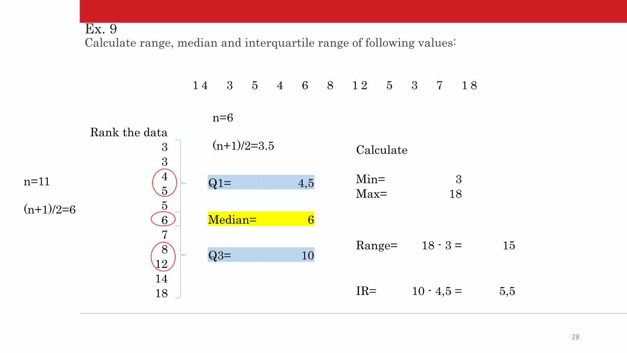
1 4 3 5 4 6 8 1 2 5 3 7 1 8

Calculate range, median and interquartile range of following values:

Rank the data

3

3

4

5

5

6

7

8

12

14

18

Q1= 4,5

Q3= 10

Median= 6

Range= 18 - 3 = 15

IR= 10 - 4,5 = 5,5

Calculate

Min= 3

Max= 18n=11

(n+1)/2=6

n=6

(n+1)/2=3.5

Ex. 9

29

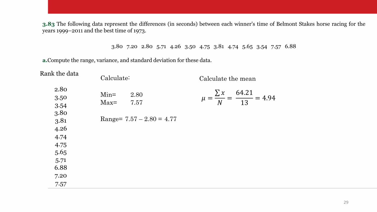
3.83 The following data represent the differences (in seconds) between each winner's time of Belmont Stakes horse racing for theyears 1999–2011 and the best time of 1973.

3.80 7.20 2.80 5.71 4.26 3.50 4.75 3.81 4.74 5.65 3.54 7.57 6.88

a.Compute the range, variance, and standard deviation for these data.

Rank the data

2.80

3.50

3.54

3.80

3.81

4.26

4.74

4.75

5.65

5.71

6.88

7.20

7.57

Range= 7.57 – 2.80 = 4.77

Calculate:

Min= 2.80

Max= 7.57𝜇 =

σ𝑥

𝑁=

64.21

13= 4.94

Calculate the mean

30

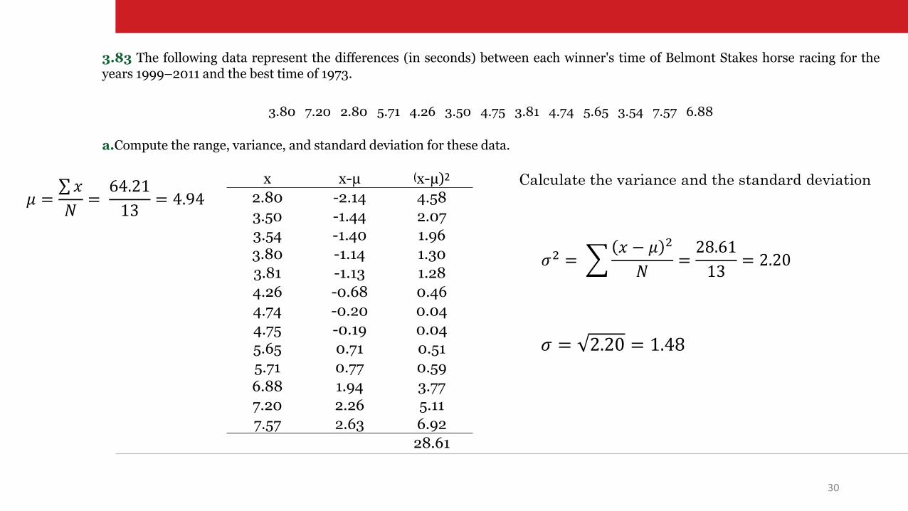
3.83 The following data represent the differences (in seconds) between each winner's time of Belmont Stakes horse racing for theyears 1999–2011 and the best time of 1973.

3.80 7.20 2.80 5.71 4.26 3.50 4.75 3.81 4.74 5.65 3.54 7.57 6.88

a.Compute the range, variance, and standard deviation for these data.

𝜇 =σ𝑥

𝑁=

64.21

13= 4.94

Calculate the variance and the standard deviationx x-µ (x-µ)2

2.80 -2.14 4.58

3.50 -1.44 2.07

3.54 -1.40 1.96

3.80 -1.14 1.30

3.81 -1.13 1.28

4.26 -0.68 0.46

4.74 -0.20 0.04

4.75 -0.19 0.04

5.65 0.71 0.51

5.71 0.77 0.59

6.88 1.94 3.77

7.20 2.26 5.11

7.57 2.63 6.92

28.61

𝜎2 = 𝑥 − 𝜇 2

𝑁=28.61

13= 2.20

𝜎 = 2.20 = 1.48

31

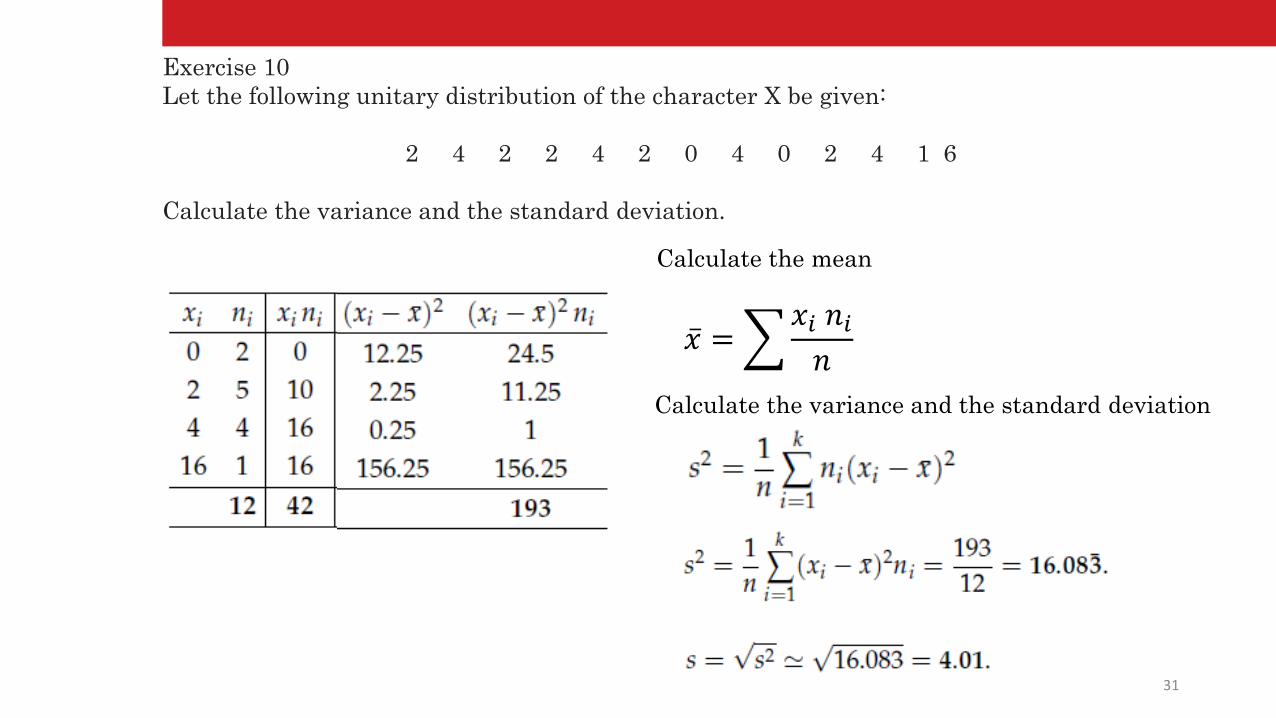
Exercise 10

Let the following unitary distribution of the character X be given:

2 4 2 2 4 2 0 4 0 2 4 1 6

Calculate the variance and the standard deviation.

ҧ𝑥 = 𝑥𝑖 𝑛𝑖𝑛

Calculate the mean

Calculate the variance and the standard deviation

32

33

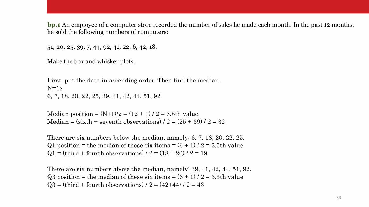
bp.1 An employee of a computer store recorded the number of sales he made each month. In the past 12 months, he sold the following numbers of computers:

51, 20, 25, 39, 7, 44, 92, 41, 22, 6, 42, 18.

Make the box and whisker plots.

First, put the data in ascending order. Then find the median.

N=12

6, 7, 18, 20, 22, 25, 39, 41, 42, 44, 51, 92

Median position = (N+1)/2 = (12 + 1) / 2 = 6.5th value

Median = (sixth + seventh observations) / 2 = (25 + 39) / 2 = 32

There are six numbers below the median, namely: 6, 7, 18, 20, 22, 25.

Q1 position = the median of these six items = (6 + 1) / 2 = 3.5th value

Q1 = (third + fourth observations) / 2 = (18 + 20) / 2 = 19

There are six numbers above the median, namely: 39, 41, 42, 44, 51, 92.

Q3 position = the median of these six items = (6 + 1) / 2 = 3.5th value

Q3 = (third + fourth observations) / 2 = (42+44) / 2 = 43

34

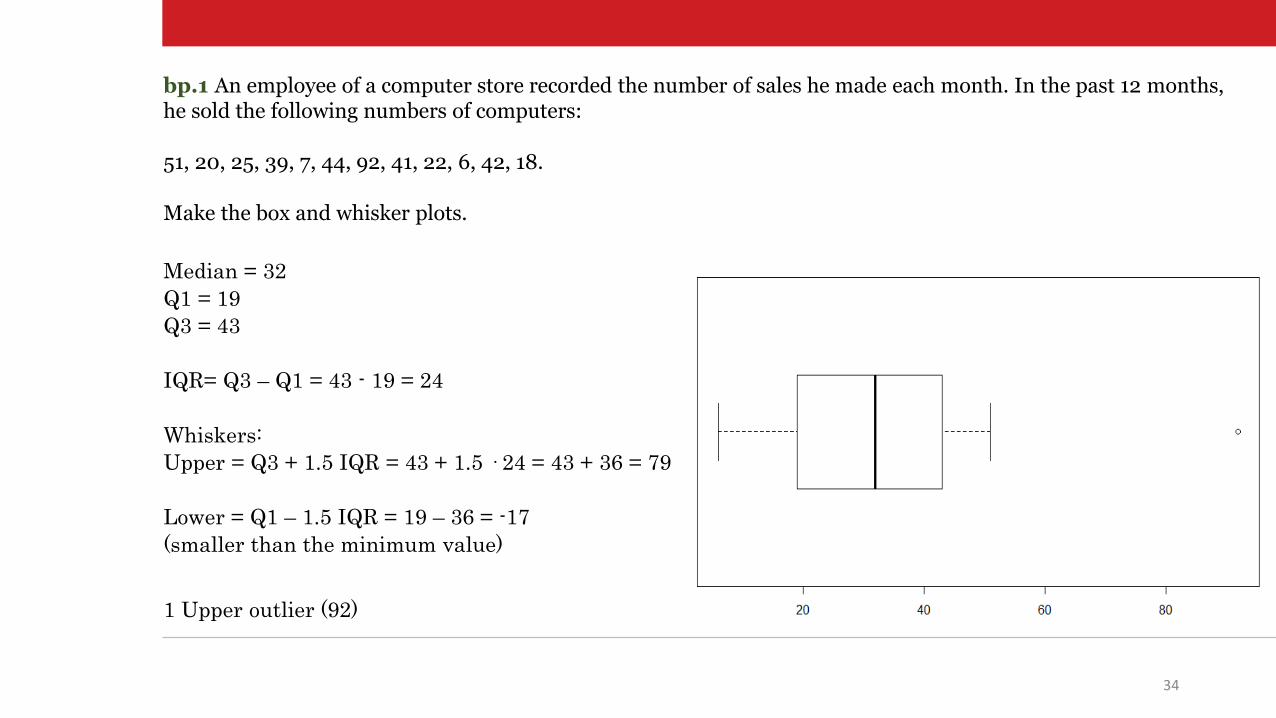
bp.1 An employee of a computer store recorded the number of sales he made each month. In the past 12 months, he sold the following numbers of computers:

51, 20, 25, 39, 7, 44, 92, 41, 22, 6, 42, 18.

Make the box and whisker plots.

Median = 32

Q1 = 19

Q3 = 43

IQR= Q3 – Q1 = 43 - 19 = 24

Whiskers:

Upper = Q3 + 1.5 IQR = 43 + 1.5 · 24 = 43 + 36 = 79

Lower = Q1 – 1.5 IQR = 19 – 36 = -17

(smaller than the minimum value)

1 Upper outlier (92)

35

(𝑛 + 1)

2=

12

2= 6

Ex. 6

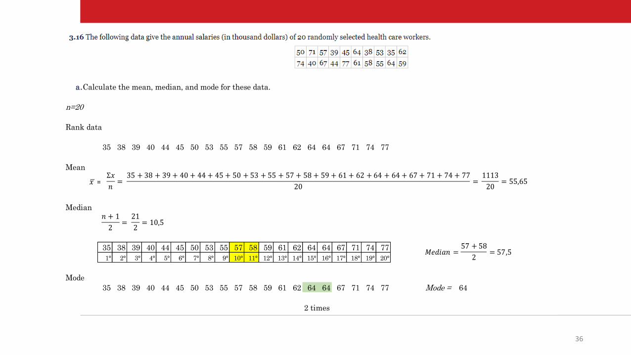
36

a.Calculate the mean, median, and mode for these data.

n=20

Rank data

35 38 39 40 44 45 50 53 55 57 58 59 61 62 64 64 67 71 74 77

Mean

Median

35 38 39 40 44 45 50 53 55 57 58 59 61 62 64 64 67 71 74 77

1° 2° 3° 4° 5° 6° 7° 8° 9° 10° 11° 12° 13° 14° 15° 16° 17° 18° 19° 20°

Mode

35 38 39 40 44 45 50 53 55 57 58 59 61 62 64 64 67 71 74 77 Mode = 64

2 times

b.Calculate the 15% trimmed mean for these data.

n=20*15%=20*0,15= 3

Drop 3 values from each end

35 38 39 40 44 45 50 53 55 57 58 59 61 62 64 64 67 71 74 77

1° 2° 3° 4° 5° 6° 7° 8° 9° 10° 11° 12° 13° 14° 15° 16° 17° 18° 19° 20°

Trimmed mean=

𝑥 = 𝑥

𝑛=

35 + 38 + 39 + 40 + 44 + 45 + 50 + 53 + 55 + 57 + 58 + 59 + 61 + 62 + 64 + 64 + 67 + 71 + 74 + 77

20=

1113

20= 55,65

𝑛 + 1

2=

21

2= 10,5

𝑒 𝑎𝑛 =57 + 58

2= 57,5

𝑥

𝑛=

40 + 44 + 45 + 50 + 53 + 55 + 57 + 58 + 59 + 61 + 62 + 64 + 64 + 67

14=

779

14= 55,64