QUANTITATIVE METHODS - NOUN

1

NATIONAL OPEN UNIVERSITY OF NIGERIA

QUANTITATIVE METHODS

ENT704

Department of Entreprenuerial Studies

FACULTY OF MANAGEMENT SCIENCES

COURSE GUIDE

Course Developers:

DR. AKINGBADE WAHEED

Lagos State University, Ojo

&

SUFIAN JELILI BABATUNDE

National Open University of Nigeria

2

NATIONAL OPEN UNIVERSITY OF NIGERIA National Open University of Nigeria

Headquarters

91, Cadastral Zone University Village Jabi-Abuja

Nigeria

e-mail: [email protected]

URL: www.nou.edu.ng

National Open University of Nigeria 2014

First Printed

ISBN:

All Rights Reserved

Printed by …………….. For

National Open University of Nigeria Multimedia Technology in Teaching and Learning

3

CONTENT

Introduction- - - - - - - - - - - 4

What you will learn in this course- - - - - - - 4

Course Content- - - - - - - - - - 4

Course Aims- - - - - - - - - - 5

Course Objectives- - - - - - - - - - 5

Working Through This Course- - - - - - - - 6

Course Materials- - - - - - - - - - 6

Study Units - - - - - - - - - - 6

References and Other Resources- - - - - - - - 7

Assignment File- - - - - - - - - - 7

Presentation Schedule- - - - - - - - - 7

Assessment- - - - - - - - - - - 7

Tutor-Marked Assignments (TMAs)- - - - - - - 8

Final Examination and Grading- - - - - - - - 8

Course Marking Scheme- - - - - - - - - 8

Course Overview- - - - - - - - - - 8

How to Get the Most From This Course- - - - - - - 9

Tutors and Tutorials- - - - - - - - - 11

Conclusion- - - - - - - - - - - 12

4

Introduction

ENT704: Quantitative Methods is a two credit course for students offering Postgraduate

Diploma in Entrepreneurial Studies in the Faculty of Management Science.

The course will consist of Sixteen (16) units, that is, four (4) modules. The material has

been developed to suit postgraduate students in Entrepreneurial Studies at the National

Open University of Nigeria (NOUN) by using an approach that treats Quantitative

Methods.

A student who successfully completes the course will surely be in a better position to

manage operations of organizations in both private and public organizations.

The course guide tells you briefly what the course is about, what course materials you will

be using and how you can work your way through these materials. It suggests some general

guidelines for the amount of time you are likely to spend on each unit of the course in order

to complete it successfully. It also gives you some guidance on your tutor-marked

assignments. Detailed information on tutor-marked assignment is found in the separate

assignment file which will be available in due course.

What you will learn in this Course

The course is made up of sixteen units, covering areas such as:

This course will introduce you to some fundamental aspects of Elements of Decision

Analysis, Types of Decision Situations, Decision Trees, Operational Research Approach

to Decision Analysis, Systems and system Analysis, Modelling in OR, Simulation, Cases

for OR Analysis, Mathematical Programming, Transportation Model, Assignment Model,

Conflict Analysis and Game Theory, Project Management, Inventory Control, Sequencing.

Course Content

The course aims, among others, are to give you an understanding of the intricacies of

Quantitative Methods and how to apply such knowledge in making real life decisions, and

managing production and operations units in both private and public enterprises.

Course Aim

The aims of the course will be achieved by your ability to:

Identify and explain Elements of Decision Analysis;

Identify and use various criteria for solving problems in different decision

situations;

5

discuss the decision tree and solve problems involving the general decision tree and

the secretary problem;

Trace the history and evolution of operation research OR;

Explain the different approaches to decision analysis;

discuss the concept of system analysis and identify the various categories of

systems;

Describe model and analyse the different types of models;

Defined simulation and highlight the various types of simulation models;

Solve different types of problems involving Linear Programming;

Explain what transportation problem is all about and solve transportation problems;

Discuss the elements of assignment problem solve decision problems using various

assignment methods;

Apply various techniques in solving gaming problems.

Solving inventory problem using the Critical Path Methods (CPM) and the

Programme evaluation and Review Techniques (PERT);

Identify and solve problems using the sequencing techniques.

Identify and solve Integer programming

COURSE OBJECTIVES

At the end of this course, you should be able to:

Identify and explain Elements of Decision Analysis;

Identify and use various criteria for solving problems in different decision

situations;

discuss the decision tree and solve problems involving the general decision tree and

the secretary problem;

Trace the history and evolution of operation research OR;

Explain the different approaches to decision analysis;

discuss the concept of system analysis and identify the various categories of

systems;

Describe model and analyse the different types of models;

Defined simulation and highlight the various types of simulation models;

Solve different types of problems involving Linear Programming;

Explain what transportation problem is all about and solve transportation problems;

Discuss the elements of assignment problem solve decision problems using various

assignment methods;

Apply various techniques in solving gaming problems.

Solving inventory problem using the Critical Path Methods (CPM) and the

Programme evaluation and Review Techniques (PERT);

Identify and solve problems using the sequencing techniques.

Working through the Course

6

To successfully complete this course, you are required to read the study units, referenced

books and other materials on the course.

Each unit contains self-assessment exercises in addition to Tutor Marked Assessments

(TMAs). At some points in the course, you will be required to submit assignments for

assessment purposes. At the end of the course there is a final examination. This course

should take about 20 weeks to complete and some components of the course are outlined

under the course material subsection.

Course Materials

The major component of the course, what you have to do and how you should allocate your

time to each unit in order to complete the course successfully on time are listed follows:

1. Course Guide

2. Study Units

3. Textbooks

4. Assignment File

5. Presentation schedule

Study Units

There are four modules of 16 units in this course, which should be studied carefully. These

are:

MODULE ONE

Unit 1: Elements of Decision Analysis

Unit 2: Types of Decision Situations

Unit 3: Decision Trees

Unit 4: Operational Research Approach to Decision Analysis

MODULE TWO

Unit 5: Systems and System Analysis

Unit 6: Modelling in Operations Research

Unit 7: Simulation

Unit 8: Cases for Operations Research Analysis

MODULE THREE

Unit 9: Mathematical Programming (Linear Programming)

7

Unit 10: Transportation Model

Unit 11: Assignment Model

Unit 12: Games Theory

MODULE FOUR

Unit 13: Project Management

Unit 14: Inventory Control

Unit 15: Sequencing

Unit 16: Case Analysis

References and Other Resources

Every unit contains a list of references and further reading. Try to get as many as possible

of those textbooks and materials listed. The textbooks and materials are meant to deepen

your knowledge of the course.

Assignment File

There are many assignments in this course and you are expected to do all of them by

following the schedule prescribed for them in terms of when to attempt the homework and

submit same for grading by your Tutor.

Presentation Schedule

The Presentation Schedule included in your course materials gives you the important dates

for the completion of tutor-marked assignments and attending tutorials. Remember, you

are required to submit all your assignments by the due date. You should guard against

falling behind in your work.

Assessment

Your assessment will be based on tutor-marked assignments (TMAs) and a final

examination which you will write at the end of the course.

Tutor-Marked Assignments (TMAs)

Assignment questions for the 16 units in this course are contained in the Assignment File.

You will be able to complete your assignments from the information and materials

contained in your set books, reading and study units. However, it is desirable that you

demonstrate that you have read and researched more widely than the required minimum.

You should use other references to have a broad viewpoint of the subject and also to give

you a deeper understanding of the subject.

When you have completed each assignment, send it, together with a TMA form, to your

tutor. Make sure that each assignment reaches your tutor on or before the deadline given

8

in the Presentation File. If for any reason, you cannot complete your work on time, contact

your tutor before the assignment is due to discuss the possibility of an extension.

Extensions will not be granted after the due date unless there are exceptional

circumstances. The TMAs usually constitute 30% of the total score for the course.

Final Examination and Grading

The final examination will be of two hours' duration and have a value of 70% of the total

course grade. The examination will consist of questions which reflect the types of self-

assessment practice exercises and tutor-marked problems you have previously

encountered. All areas of the course will be assessed

You should use the time between finishing the last unit and sitting for the examination to

revise the entire course material. You might find it useful to review your self-assessment

exercises, tutor-marked assignments and comments on them before the examination. The

final examination covers information from all parts of the course.

Course Marking Scheme

The Table presented below indicates the total marks (100%) allocation.

Assessment Marks

Assignment (Three assignment marked) 30%

Final Examination 70%

Total 100%

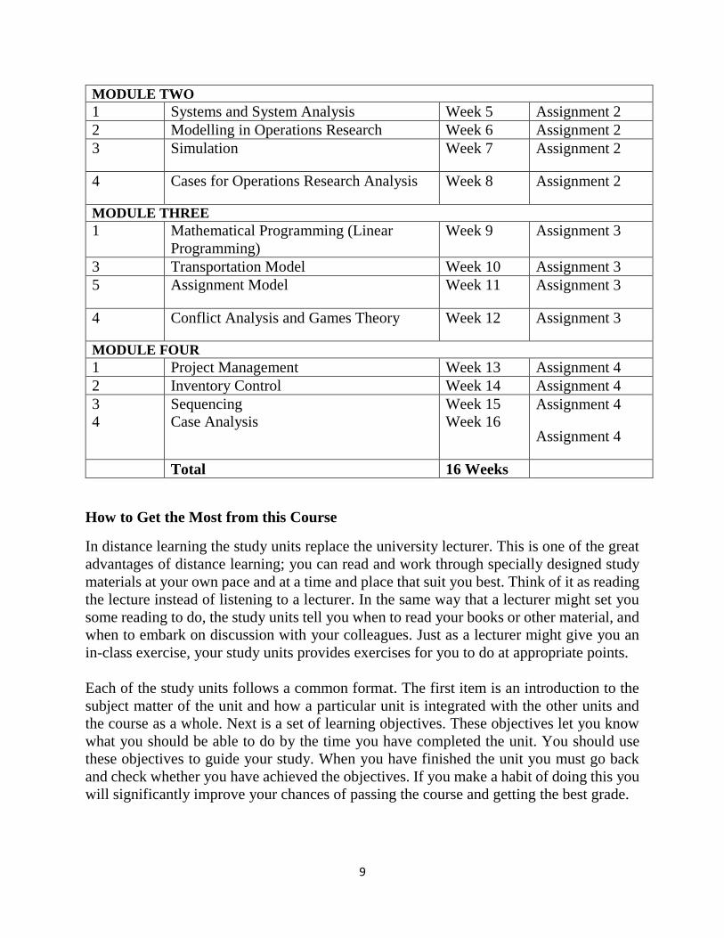
Course Overview

The Table presented below indicates the units, number of weeks and assignments to be

taken by you to successfully complete the course, Operations Research (ENT704).

Units Title of Work Week’s

Activities

Assessment

(end of unit)

Course Guide MODULE ONE

1 Elements of Decision Analysis Week 1 Assignment 1

2 Types of Decision Situations Week 2 Assignment 1

3 Decision Trees Week 3 Assignment 1

4 Operatonal Research Approach to

Decision Analysis

Week 4 Assignment 1

9

MODULE TWO

1 Systems and System Analysis Week 5 Assignment 2

2 Modelling in Operations Research Week 6 Assignment 2

3 Simulation Week 7 Assignment 2

4 Cases for Operations Research Analysis Week 8 Assignment 2

MODULE THREE

1 Mathematical Programming (Linear

Programming)

Week 9 Assignment 3

3 Transportation Model Week 10 Assignment 3

5 Assignment Model Week 11 Assignment 3

4 Conflict Analysis and Games Theory Week 12 Assignment 3

MODULE FOUR

1 Project Management Week 13 Assignment 4

2 Inventory Control Week 14 Assignment 4

3

4

Sequencing

Case Analysis

Week 15

Week 16

Assignment 4

Assignment 4

Total 16 Weeks

How to Get the Most from this Course

In distance learning the study units replace the university lecturer. This is one of the great

advantages of distance learning; you can read and work through specially designed study

materials at your own pace and at a time and place that suit you best. Think of it as reading

the lecture instead of listening to a lecturer. In the same way that a lecturer might set you

some reading to do, the study units tell you when to read your books or other material, and

when to embark on discussion with your colleagues. Just as a lecturer might give you an

in-class exercise, your study units provides exercises for you to do at appropriate points.

Each of the study units follows a common format. The first item is an introduction to the

subject matter of the unit and how a particular unit is integrated with the other units and

the course as a whole. Next is a set of learning objectives. These objectives let you know

what you should be able to do by the time you have completed the unit. You should use

these objectives to guide your study. When you have finished the unit you must go back

and check whether you have achieved the objectives. If you make a habit of doing this you

will significantly improve your chances of passing the course and getting the best grade.

10

The main body of the unit guides you through the required reading from other sources.

This will usually be either from your set books or from a readings section. Self-assessments

are interspersed throughout the units, and answers are given at the ends of the units.

Working through these tests will help you to achieve the objectives of the unit and prepare

you for the assignments and the examination. You should do each self-assessment exercises

as you come to it in the study unit. Also, ensure to master some major historical dates and

events during the course of studying the material.

The following is a practical strategy for working through the course. If you run into any

trouble, consult your Tutor. Remember that your Tutor's job is to help you. When you need

help, don't hesitate to call and ask your Tutor to provide the help.

1. Read this Course Guide thoroughly.

2. Organize a study schedule. Refer to the `Course overview' for more details. Note

the time you are expected to spend on each unit and how the assignments relate to

the units. Important information, e.g. details of your tutorials, and the date of the

first day of the semester is available from study centre. You need to gather together

all this information in one place, such as your dairy, a wall calendar, an iPad or a

handset. Whatever method you choose to use, you should decide on and write in

your own dates for working each unit.

3. Once you have created your own study schedule, do everything you can to stick to

it. The major reason that students fail is that they get behind with their course work.

If you get into difficulties with your schedule, please let your Tutor know before it

is too late for help.

4. Turn to Unit 1 and read the introduction and the objectives for the unit.

5. Assemble the study materials. Information about what you need for a unit is given

in the `Overview' at the beginning of each unit. You will also need both the study

unit you are working on and one of your set books on your desk at the same time.

6. Work through the unit. The content of the unit itself has been arranged to provide a

sequence for you to follow. As you work through the unit you will be instructed to

read sections from your set books or other articles. Use the unit to guide your

reading.

7. Up-to-date course information will be continuously delivered to you at the study

centre.

8. Work before the relevant due date (about 4 weeks before due dates), get the

Assignment File for the next required assignment. Keep in mind that you will learn

a lot by doing the assignments carefully. They have been designed to help you meet

the objectives of the course and, therefore, will help you pass the exam. Submit all

assignments no later than the due date.

9. Review the objectives for each study unit to confirm that you have achieved them.

If you feel unsure about any of the objectives, review the study material or consult

your Tutor.

11

10. When you are confident that you have achieved a unit's objectives, you can then

start on the next unit. Proceed unit by unit through the course and try to space your

study so that you keep yourself on schedule.

11. When you have submitted an assignment to your Tutor for marking, do not wait for

its return `before starting on the next units. Keep to your schedule. When the

assignment is returned, pay particular attention to your Tutor's comments, both on

the tutor-marked assignment form and also written on the assignment. Consult your

Tutor as soon as possible if you have any questions or problems.

12. After completing the last unit, review the course and prepare yourself for the final

examination. Check that you have achieved the unit objectives (listed at the

beginning of each unit) and the course objectives (listed in this Course Guide).

Tutors and Tutorials

There are some hours of tutorials (2-hours sessions) provided in support of this course. You

will be notified of the dates, times and location of these tutorials, together with the name

and phone number of your Tutor, as soon as you are allocated a Tutorial group.

Your tutor will mark and comment on your assignments, keep a close watch on your

progress and on any difficulties you might encounter, and provide assistance to you during

the course. You must mail your tutor-marked assignments to your tutor well before the due

date (at least two working days are required). They will be marked by your Tutor and

returned to you as soon as possible.

Do not hesitate to contact your Tutor by telephone, e-mail, or discussion board if you need

help. The following might be circumstances in which you would find help necessary.

Contact your Tutor if.

• You do not understand any part of the study units or the assigned readings

• You have difficulty with the self-assessment exercises

• You have a question or problem with an assignment, with your Tutor's comments on an

assignment or with the grading of an assignment.

You should try your best to attend the tutorials. This is the only chance to have face to face

contact with your Tutor and to ask questions which are answered instantly. You can raise

any problem encountered in the course of your study. To gain the maximum benefit from

course tutorials, prepare a question list before attending them. You will learn a lot from

participating in discussions actively.

Conclusion

12

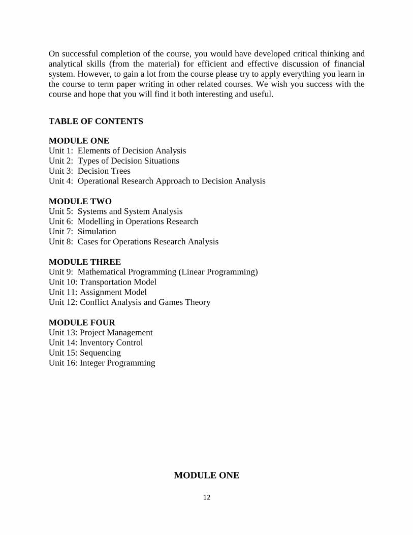
On successful completion of the course, you would have developed critical thinking and

analytical skills (from the material) for efficient and effective discussion of financial

system. However, to gain a lot from the course please try to apply everything you learn in

the course to term paper writing in other related courses. We wish you success with the

course and hope that you will find it both interesting and useful.

TABLE OF CONTENTS

MODULE ONE

Unit 1: Elements of Decision Analysis

Unit 2: Types of Decision Situations

Unit 3: Decision Trees

Unit 4: Operational Research Approach to Decision Analysis

MODULE TWO

Unit 5: Systems and System Analysis

Unit 6: Modelling in Operations Research

Unit 7: Simulation

Unit 8: Cases for Operations Research Analysis

MODULE THREE

Unit 9: Mathematical Programming (Linear Programming)

Unit 10: Transportation Model

Unit 11: Assignment Model

Unit 12: Conflict Analysis and Games Theory

MODULE FOUR

Unit 13: Project Management

Unit 14: Inventory Control

Unit 15: Sequencing

Unit 16: Integer Programming

MODULE ONE

13

UNIT 1: ELEMENTS OF DECISION ANALYSIS

1.0 Introduction

2.0 Objectives

3.0 Main Content

3.1 What is a Decision?

3.2 Who is a Decision Maker?

3.3 Decision Analysis

3.4 Components of Decision Making

3.4.1 Decision Alternatives

3.4.2 States of Nature

3.4.3 The Decision

3.4.4 Decision Screening Criteria

3.5 Phases of Decision Analysis

3.6 Errors that can occur in Decision Making

4.0 Conclusion

5.0 Summary

6.0 Tutor Marked Assignment

7.0 References

1.0 INTRODUCTION

Business Decision Analysis takes its roots from Operations Research (OR). Operation

Research as we will learn later is the application of scientific method by interdisciplinary

teams to problems solving and the control of organized (Man-Machine) systems so as to

provide solution which best serve the purpose of the organization as a whole (Ackoff and

Sisieni 1991). In other words, Operations Research makes use of scientific methods and

tools to provide optimum or best solutions to problems in the organization. Organisations

are usually faced with the problem of deciding what to do; how to do it, where to do it, for

whom to do it etc. But before any action can be taken, it is important to properly analyse a

situation with a view to finding out the various alternative courses of action that are

available to an organization.

2.0 OBJECTIVES

By the end of this study unit, you should be able to:

1. Define a decision

2. Define a decision maker

3. Describe the components of Decision making

4. Outline the structure of a decision problem

3.0 MAIN CONTENT

14

3.1 WHAT IS A DECISION?

A decision can be defined as an action to be selected according to some pre-specified rule

or strategy, out of several available alternatives, to facilitate a future course of action. This

definition suggests that there are several alternative courses of action available, which

cannot be pursued at the same time. Therefore, it is imperative to choose the best alternative

base on some specified rule or strategy.

3.2 WHO IS A DECISION MAKER?

A decision maker is one who takes decision. It could be an individual or a group of

individuals. It is expected that a good decision maker should be skilled in art of making

decisions.

3.3 DECISION ANALYSIS

Decision making is a very important and necessary aspect of every human endeavour. In

life, we are faced with decision problems in everything we do. Individuals make decisions

daily on what to do, what to wear, what to eat etc. Every human being is assumed to be a

rational decision maker who takes decisions to improve his/her wellbeing. In business,

management have to make decision on daily bases on ways to improve business

performance. But unlike individual decision making, organizational or business decision

making is a very complex process considering the various factors involved. It is easy to

take decision for simple situation but when it gets complex, it is better not to rely on

intuition. Decision theory proves useful when it comes to issues of risk and uncertainty

(Adebayo et al 2010).

3.4 COMPONENTS OF DECISION MAKING

Earlier, we stated that complex decision problem involve risk and an uncertainty and as

such, certain logic, rules, procedures should be applied when analysing such situation. The

major components that constitute risk and uncertainty in decision making are:

Decision alternatives

States of Nature

The decision itself

Decision screening criteria

We now briefly discourse each of these components.

3.4.1 DECISION ALTERNATIVES

These are alternative courses of action available to the decision maker. The alternatives

should be feasible, and evaluating them will depend on the availability of a well-defined

objective. Alternative courses of action may also be seen as strategies or options from

which the decision maker must choose from. It is due to the existence of several alternatives

that the decision problem arises. If there were only one course of action, then there will be

no decision problem.

Alternatives present themselves as:

15

(a) Choices of products to manufacture,

(b) Transportation roots to be taken,

(c) Choice of customer to serve,

(d) Financing option for a new project,

(e) How to order job into machines, etc.

3.4.2. STATES OF NATURE A state of nature is a future occurrence for which the decision maker has no control over.

All the time a decision is made, the decision maker is not certain which states of nature

will occur in future, and he has no influence over them (Taylor III, 2007). For instance, if

a company has a contract to construct a 30km road, it may complete the construction of the

full stretch of road in six months in line with a laid down plan. But this plan will be hinged

on the possibility that it does not rain in the next six months. However, if there is consistent

heavy rain for the first three months, it may delay the progress of work significantly and as

a result, prolong the completion date of the project. But if actually there is no occurrence

of heavy rainfall, the company is likely to complete the road as scheduled.

3.4.3. THE DECISION

The decision itself is a choice which is arrived at after considering all alternatives available

given an assumed future state of nature. In the view of Dixon-Ogbechi (2001), “A good

decision is one that is based on logic, considers all available data, and possible alternative

and employs quantitative technique” she further noted that, occasionally, a good decision

may yield a bad result, but if made properly, may result in successful outcome in the long

run.

3.4.4 DECISION SCREENING CRITERIA

In the section above, we mentioned that the decision itself is a choice which is arrived at

after considering all other alternatives. Consideration of alternative courses of action is not

done arbitrarily, it is done using some standardize logic or methodology, or criterion. These

criteria form the basis upon which alternatives are compared. The strategy or alternative

which is finally selected is the one associated with the most attractive outcome. The degree

of attractiveness will depend on the objective of the decision maker and the criterion used

for analysis (Ihemeje 2002).

IN TEXT QUESTION

Define a decision.

Who is a decision maker?\

What do you understand by states of nature?

What is decision analysis?

List the two most prominent business objectives.

3.5 PHASES OF DECISION ANALYSIS

16

The process of analysing decision can be grouped into four phases. These four phases from

what is known as the decision analysis cycle. They are presented as follows:

Deterministic Analysis Phase: This phase accounts for certainties rather than

uncertainties. Here, graphical and diagrammatic models like influence diagrams and

flow charts can be translated into mathematical models.

Necessary tools are used for predicting consequences of alternatives and for

evaluating decision alternatives.

Probabilistic Analysis: Probabilistic analyses cater for uncertainties in the decision

making process. We can use the decision tree as a tool for probabilistic analysis.

Evaluation Phase: At the phase, the alternative strategies are evaluated to enable

one identify the decision outcomes that correspond to sequence of decisions and

events.

3.6 ERRORS THAT CAN OCCUR IN DECISION MAKING

The following are possible errors to guide against when making decisions.

Inability to identify and specify key objectives: Identifying specific objectives gives

the decision maker a clear sense of direction.

Focusing on the wrong problem: This could create distraction and will lead the

decision maker to an inappropriate solution.

Not giving adequate thoughts to trade-offs which may be highly essential to the

decision making process.

4.0 CONCLUSION

In life, decisions are made every moment a human being acts or refuses to act. Decision

can be made either as single individuals or as group of individuals or as organizations.

Those decisions are made in order to meet laid down goals and objectives which in most

cases are aim to bring about improvement in fortunes. However, most organizational

decisions are complex and cannot be made using common sense. In that case, scientific

methods, tools, procedures, techniques and processes are employed to analyse the problems

with a view to arriving at optimum solution that will meet the objectives of the

organization.

5.0 SUMMARY

In this unit, the elements of decision analysis were discussed. It began with defining a

decision, and who a decision maker is. Further, it considers the components of Decision

making, structure of a decision problem and finally errors that can occur in decision

making. This unit provides us with concepts that will help us in understanding the

subsequent units and modules.

6.0 TUTOR MARKED ASSIGNMENT

Who is a Decision Maker?

Define Decision Analysis.

List and explain the components of decision.

17

7.0 REFERENCES

Ackoff, R., and Sisieni, M. (1991). Fundamentals of Operations Research, New York: John

Wiley and Sons Inc.

Adebayo, O.A., Ojo, O., and Obamire, J.K. (2006). Operations Research in Decision

Analysis, Lagos: Pumark Nigeria Limited.

Churchman, C.W. et al (1957). Introduction to Operations Research, New York: John

Wiley and Sons Inc.

Howard, A. (2004). Speaking of Decisions: Precise Decision Language. Decision Analysis,

Vol. 1 No. 2, June).

Ihemeje, J.C. (2002). Fundamentals of Business Decision Analysis, Ibadan: Sibon Books

Limited.

Shamrma, J.K. (2009). Operations Research Theory & Application

Kingsley, U.U (2014). Analysis for Business Decision, National Open Univeristy of

Nigeria.

18

UNIT 2: TYPES OF DECISION SITUATIONS

1.0 Introduction

2.0 Objectives

3.0 Main Content

3.1 Elements of Decision Situation

3.2 Types of Decision Situations

3.2.1 Decision Making Under Condition of Certainty

3.2.2 Decision Making Under Conditions of Uncertainty

3.2.3 Decision Making Under Conditions of Risk

3.2.4 Decision Under Conflict

4.0 Conclusion

5.0 Summary


7.0 References

1.0 INTRODUCTION

Recall that in the previous unit we presented five decision criteria – Maximax, Maximin,

Laplace’s, Minimax Regret, and Hurwicz criterion. We also stated that the criteria are used

foranalysing decision situations under uncertainty. In this unit, we shall delve fully into

considering these situations and learn how we can use different techniques in analysing

problems in certian decision situations i.e Certainty, Uncertainty, Risk, and Conflict

situations.

2.0 OBJECTIVES After studying this unit, you should be able to

Identify the four conditions under which decisions can be made

Describe each decision situation

Identify the techniques for making decision under each decision situation

Solve problems under each of the decision situation

3.0 MAIN CONTENT

3.1 ELEMENTS OF DECISION SITUATION

Dixon – Ogbechi (2001) presents the following elements of Decision Situation:

1 The Decision Maker: The person or group of persons making the decision.

2 Value System: This is the particular preference structure of the decision maker.

3 Environmental Factors: These are also called states of nature. They can be

i. Political v Cultural factors

ii. Legal vi. Technological factors

iii. Economic factors vii Natural Disasters

iv. Social factors

19

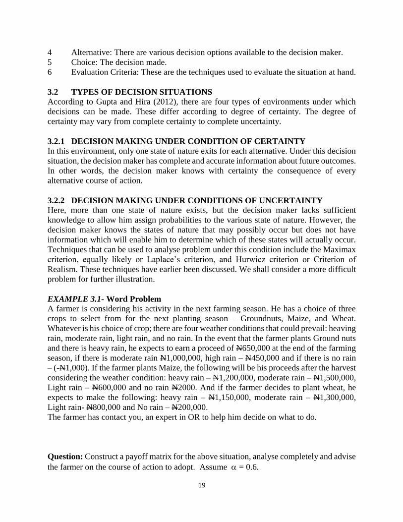
4 Alternative: There are various decision options available to the decision maker.

5 Choice: The decision made.

6 Evaluation Criteria: These are the techniques used to evaluate the situation at hand.

3.2 TYPES OF DECISION SITUATIONS According to Gupta and Hira (2012), there are four types of environments under which

decisions can be made. These differ according to degree of certainty. The degree of

certainty may vary from complete certainty to complete uncertainty.

3.2.1 DECISION MAKING UNDER CONDITION OF CERTAINTY In this environment, only one state of nature exits for each alternative. Under this decision

situation, the decision maker has complete and accurate information about future outcomes.

In other words, the decision maker knows with certainty the consequence of every

alternative course of action.

3.2.2 DECISION MAKING UNDER CONDITIONS OF UNCERTAINTY

Here, more than one state of nature exists, but the decision maker lacks sufficient

knowledge to allow him assign probabilities to the various state of nature. However, the

decision maker knows the states of nature that may possibly occur but does not have

information which will enable him to determine which of these states will actually occur.

Techniques that can be used to analyse problem under this condition include the Maximax

criterion, equally likely or Laplace’s criterion, and Hurwicz criterion or Criterion of

Realism. These techniques have earlier been discussed. We shall consider a more difficult

problem for further illustration.

EXAMPLE 3.1- Word Problem

A farmer is considering his activity in the next farming season. He has a choice of three

crops to select from for the next planting season – Groundnuts, Maize, and Wheat.

Whatever is his choice of crop; there are four weather conditions that could prevail: heaving

rain, moderate rain, light rain, and no rain. In the event that the farmer plants Ground nuts

and there is heavy rain, he expects to earn a proceed of N650,000 at the end of the farming

season, if there is moderate rain N1,000,000, high rain – N450,000 and if there is no rain

– (-N1,000). If the farmer plants Maize, the following will be his proceeds after the harvest

considering the weather condition: heavy rain – N1,200,000, moderate rain – N1,500,000,

Light rain – N600,000 and no rain N2000. And if the farmer decides to plant wheat, he

expects to make the following: heavy rain – N1,150,000, moderate rain – N1,300,000,

Light rain- N800,000 and No rain – N200,000.

The farmer has contact you, an expert in OR to help him decide on what to do.

Question: Construct a payoff matrix for the above situation, analyse completely and advise

the farmer on the course of action to adopt. Assume = 0.6.

20

Solution

First, construct a contingency matrix from the above problem.

Contingency Matrix 1a

Weather

Condition

Alternative

Crops

Heavy Rain (S1)

N

Moderate Rain (S2)

N

Light Rain Rain (S3)

N

No Rain Rain (S4)

N

Groundnut (d1) 750,000 1,000,000 450,000 -1,000

Maize (d2) 1,200,000 1,500,000 600,000 2,000

Wheat (d3) 1,150,000 1,300,000 800,000 -200,000

Fig. 3.1a: Pay- off Table

Contingency Matrix 1b

Weather

Condition

Alternative

Crops

(S1)

(N’ 000)

(S2)

(N ‘000)

(S3)

(N ‘000)

(S4)

(N ‘000)

Max Col Max Min

d1 750 1,000 450 -1 1,000 -1

d2 1,200 1,500 600 2 1,500 2

d3 1,150 1,300 800 -200 1,300 -200

Fig. 3.1b: Pay- off Table

Regret Matrix

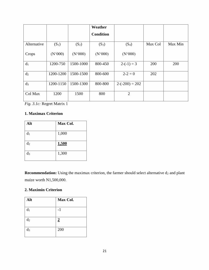
21

Weather

Condition

Alternative

Crops

(S1)

(N‘000)

(S2)

(N‘000)

(S3)

(N‘000)

(S4)

(N‘000)

Max Col Max Min

d1 1200-750 1500-1000 800-450 2-(-1) = 3 200 200

d2 1200-1200 1500-1500 800-600 2-2 = 0 202

d3 1200-1150 1500-1300 800-800 2-(-200) = 202

Col Max 1200 1500 800 2

Fig. 3.1c: Regret Matrix 1

1. Maximax Criterion

Alt Max Col.

d1 1,000

d2 1,500

d3 1,300

Recommendation: Using the maximax criterion, the farmer should select alternative d2 and plant

maize worth N1,500,000.

2. Maximin Criterion

Alt Max Col.

d1 -1

d2 2

d3 200

22

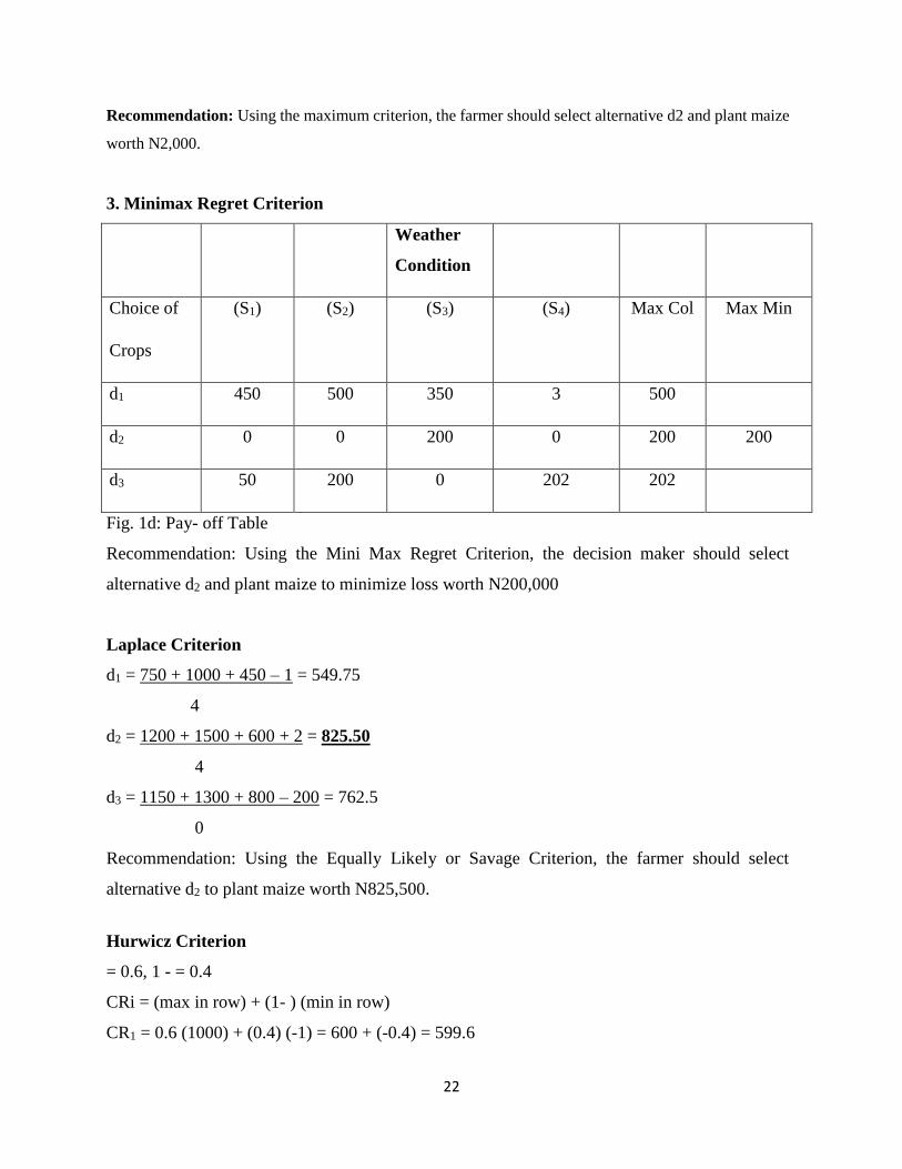
Recommendation: Using the maximum criterion, the farmer should select alternative d2 and plant maize

worth N2,000.

3. Minimax Regret Criterion

Weather

Condition

Choice of

Crops

(S1)

(S2)

(S3)

(S4)

Max Col Max Min

d1 450 500 350 3 500

d2 0 0 200 0 200 200

d3 50 200 0 202 202

Fig. 1d: Pay- off Table

Recommendation: Using the Mini Max Regret Criterion, the decision maker should select

alternative d2 and plant maize to minimize loss worth N200,000

Laplace Criterion

d1 = 750 + 1000 + 450 – 1 = 549.75

4

d2 = 1200 + 1500 + 600 + 2 = 825.50

4

d3 = 1150 + 1300 + 800 – 200 = 762.5

0

Recommendation: Using the Equally Likely or Savage Criterion, the farmer should select

alternative d2 to plant maize worth N825,500.

Hurwicz Criterion

= 0.6, 1 - = 0.4

CRi = (max in row) + (1- ) (min in row)

CR1 = 0.6 (1000) + (0.4) (-1) = 600 + (-0.4) = 599.6

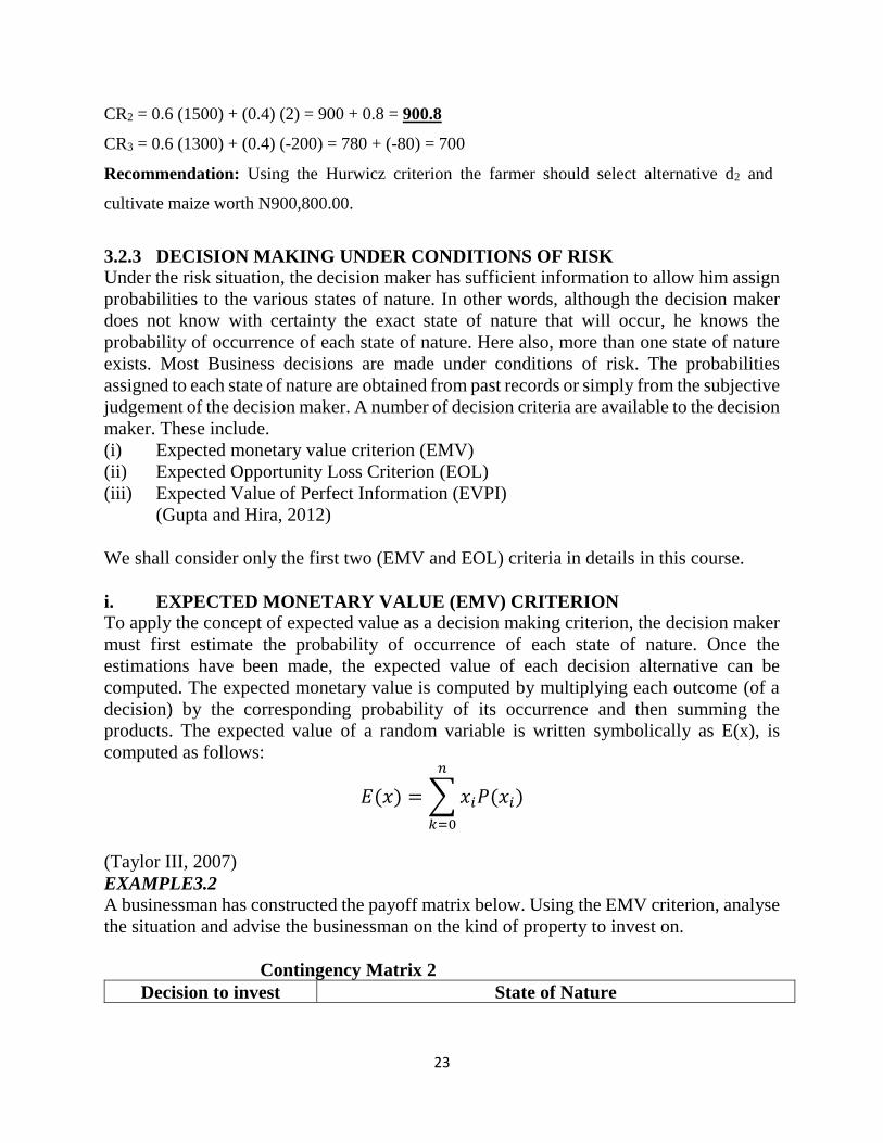
23

CR2 = 0.6 (1500) + (0.4) (2) = 900 + 0.8 = 900.8

CR3 = 0.6 (1300) + (0.4) (-200) = 780 + (-80) = 700

Recommendation: Using the Hurwicz criterion the farmer should select alternative d2 and

cultivate maize worth N900,800.00.

3.2.3 DECISION MAKING UNDER CONDITIONS OF RISK

Under the risk situation, the decision maker has sufficient information to allow him assign

probabilities to the various states of nature. In other words, although the decision maker

does not know with certainty the exact state of nature that will occur, he knows the

probability of occurrence of each state of nature. Here also, more than one state of nature

exists. Most Business decisions are made under conditions of risk. The probabilities

assigned to each state of nature are obtained from past records or simply from the subjective

judgement of the decision maker. A number of decision criteria are available to the decision

maker. These include.

(i) Expected monetary value criterion (EMV)

(ii) Expected Opportunity Loss Criterion (EOL)

(iii) Expected Value of Perfect Information (EVPI)

(Gupta and Hira, 2012)

We shall consider only the first two (EMV and EOL) criteria in details in this course.

i. EXPECTED MONETARY VALUE (EMV) CRITERION

To apply the concept of expected value as a decision making criterion, the decision maker

must first estimate the probability of occurrence of each state of nature. Once the

estimations have been made, the expected value of each decision alternative can be

computed. The expected monetary value is computed by multiplying each outcome (of a

decision) by the corresponding probability of its occurrence and then summing the

products. The expected value of a random variable is written symbolically as E(x), is

computed as follows:

𝐸(𝑥) = ∑ 𝑥𝑖𝑃(𝑥𝑖)

𝑛

𝑘=0

(Taylor III, 2007)

EXAMPLE3.2

A businessman has constructed the payoff matrix below. Using the EMV criterion, analyse

the situation and advise the businessman on the kind of property to invest on.

Contingency Matrix 2

Decision to invest State of Nature

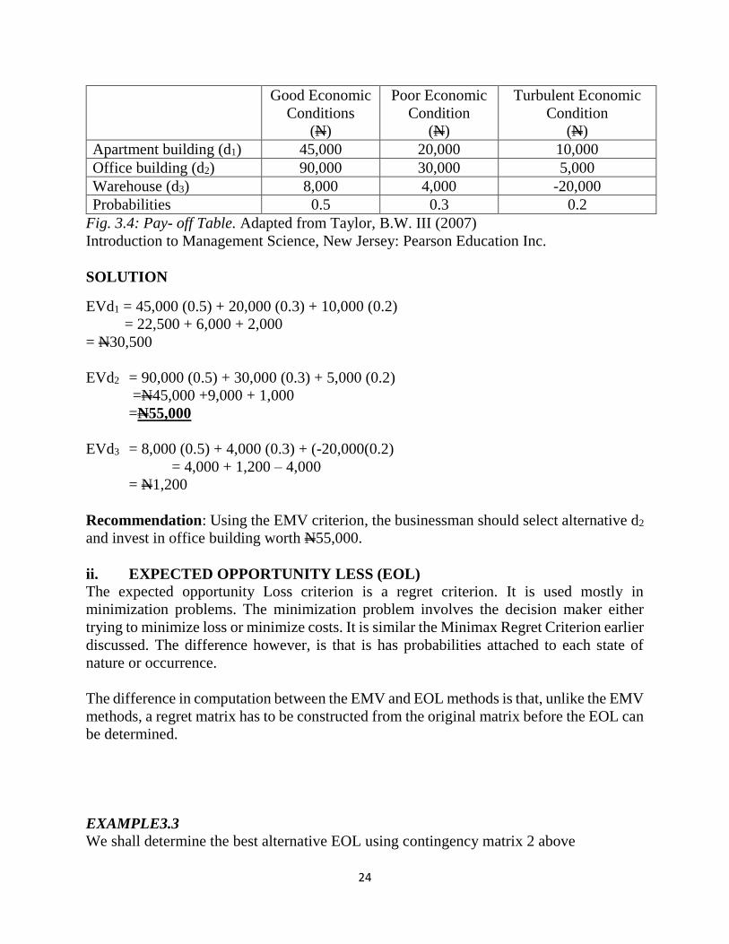
24

Good Economic

Conditions

(N)

Poor Economic

Condition

(N)

Turbulent Economic

Condition

(N)

Apartment building (d1) 45,000 20,000 10,000

Office building (d2) 90,000 30,000 5,000

Warehouse (d3) 8,000 4,000 -20,000

Probabilities 0.5 0.3 0.2

Fig. 3.4: Pay- off Table. Adapted from Taylor, B.W. III (2007)

Introduction to Management Science, New Jersey: Pearson Education Inc.

SOLUTION

EVd1 = 45,000 (0.5) + 20,000 (0.3) + 10,000 (0.2)

= 22,500 + 6,000 + 2,000

= N30,500

EVd2 = 90,000 (0.5) + 30,000 (0.3) + 5,000 (0.2)

=N45,000 +9,000 + 1,000

=N55,000

EVd3 = 8,000 (0.5) + 4,000 (0.3) + (-20,000(0.2)

= 4,000 + 1,200 – 4,000

= N1,200

Recommendation: Using the EMV criterion, the businessman should select alternative d2

and invest in office building worth N55,000.

ii. EXPECTED OPPORTUNITY LESS (EOL)

The expected opportunity Loss criterion is a regret criterion. It is used mostly in

minimization problems. The minimization problem involves the decision maker either

trying to minimize loss or minimize costs. It is similar the Minimax Regret Criterion earlier

discussed. The difference however, is that is has probabilities attached to each state of

nature or occurrence.

The difference in computation between the EMV and EOL methods is that, unlike the EMV

methods, a regret matrix has to be constructed from the original matrix before the EOL can

be determined.

EXAMPLE3.3

We shall determine the best alternative EOL using contingency matrix 2 above

25

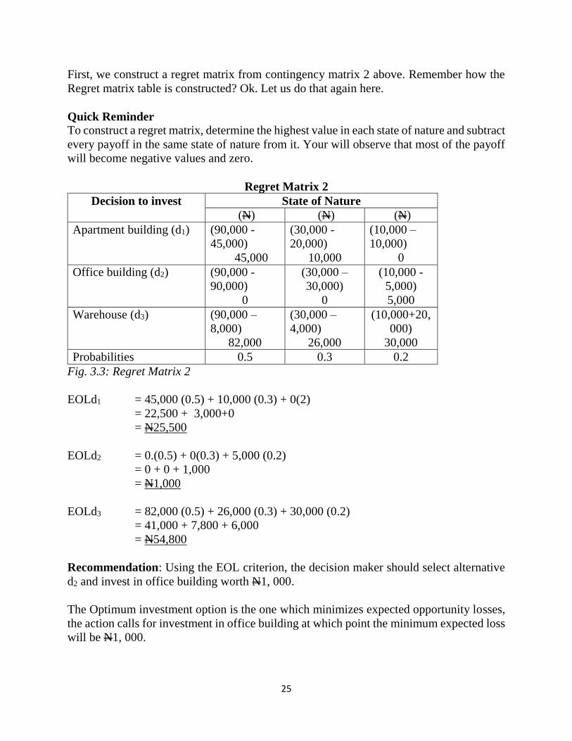
First, we construct a regret matrix from contingency matrix 2 above. Remember how the

Regret matrix table is constructed? Ok. Let us do that again here.

Quick Reminder

To construct a regret matrix, determine the highest value in each state of nature and subtract

every payoff in the same state of nature from it. Your will observe that most of the payoff

will become negative values and zero.

Regret Matrix 2


(N) (N) (N)

Apartment building (d1) (90,000 -

45,000)

45,000

(30,000 -

20,000)

10,000

(10,000 –

10,000)

0

Office building (d2) (90,000 -

90,000)

0

(30,000 –

30,000)

0

(10,000 -

5,000)

5,000

Warehouse (d3) (90,000 –

8,000)

82,000

(30,000 –

4,000)

26,000

(10,000+20,

000)

30,000


Fig. 3.3: Regret Matrix 2

EOLd1 = 45,000 (0.5) + 10,000 (0.3) + 0(2)

= 22,500 + 3,000+0

= N25,500

EOLd2 = 0.(0.5) + 0(0.3) + 5,000 (0.2)

= 0 + 0 + 1,000

= N1,000

EOLd3 = 82,000 (0.5) + 26,000 (0.3) + 30,000 (0.2)

= 41,000 + 7,800 + 6,000

= N54,800

Recommendation: Using the EOL criterion, the decision maker should select alternative

d2 and invest in office building worth N1, 000.

The Optimum investment option is the one which minimizes expected opportunity losses,

the action calls for investment in office building at which point the minimum expected loss

will be N1, 000.

26

You will notice that the decision rule under this criterion is the same with that of the

Minimax Regret criterion. This is because both methods have the same objectives that is,

the minimization of loss. They are both pessimistic in nature. However, loss minimization

is not the only form minimization problem. Minimisation problems could also be in the

form of minimisation of cost of production or investment. In analysing a problem involving

the cost of production you do not have to construct a regret matrix because the pay-off in

the table already represents cost.

NOTE: It should be pointed out that EMV and EOL decision criteria are completely

consistent and yield the same optimal decision alternative.

iii EXPECTED VALUE OF PERFECT INFORMATION

Taylor III (2007) is of the view that it is often possible to purchase additional information

regarding future events and thus make better decisions. For instance, a farmer could hire a

weather forecaster to analyse the weather conditions more accurately to determine which

weather condition will prevail during the next farming season. However, it would not be

wise for the farmer to pay more for this information than he stands to gain in extra yield

from having this information. That is, the information has some maximum yield value that

represents the limit of what the decision maker would be willing to spend. This value of

information can be computed as an expected value – hence its name, expected value of

perfect information (EVPI).

The expected value of perfect information therefore is the maximum amount a decision

maker would pay for additional information. In the view of Adebayo et al (2007), the value

of perfect information is the amount by which the profit will be increased with additional

information. It is the difference between expected value of optimum quantity under risk

and the expected value under certainty. Using the EOL criterion, the value of expected loss

will be the value of the perfect information.

Expected value of perfect information can be computed as follows

EVPI = EVwPI – EMVmax

Where

EVPI = Expected value of perfect information

EVwPI = Expected value with perfect information

EMVmax = Maximum expected monetary value or Expected value without perfect

information

(Or minimum EOL for a minimization problem)

EXAMPLE3.4

27

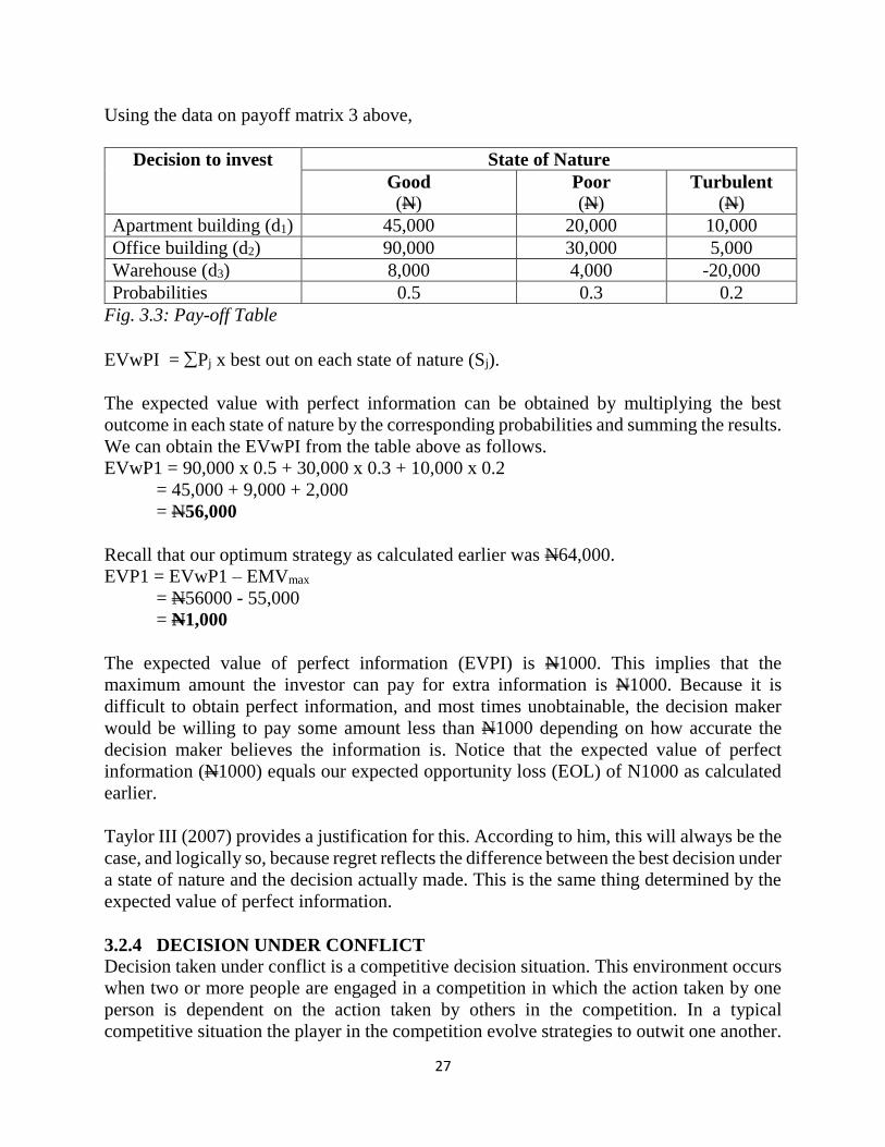
Using the data on payoff matrix 3 above,


Good

(N) Poor

(N) Turbulent

(N)

Apartment building (d1) 45,000 20,000 10,000

Office building (d2) 90,000 30,000 5,000

Warehouse (d3) 8,000 4,000 -20,000


Fig. 3.3: Pay-off Table

EVwPI = Pj x best out on each state of nature (Sj).

The expected value with perfect information can be obtained by multiplying the best

outcome in each state of nature by the corresponding probabilities and summing the results.

We can obtain the EVwPI from the table above as follows.

EVwP1 = 90,000 x 0.5 + 30,000 x 0.3 + 10,000 x 0.2

= 45,000 + 9,000 + 2,000

= N56,000

Recall that our optimum strategy as calculated earlier was N64,000.

EVP1 = EVwP1 – EMVmax

= N56000 - 55,000

= N1,000

The expected value of perfect information (EVPI) is N1000. This implies that the

maximum amount the investor can pay for extra information is N1000. Because it is

difficult to obtain perfect information, and most times unobtainable, the decision maker

would be willing to pay some amount less than N1000 depending on how accurate the

decision maker believes the information is. Notice that the expected value of perfect

information (N1000) equals our expected opportunity loss (EOL) of N1000 as calculated

earlier.

Taylor III (2007) provides a justification for this. According to him, this will always be the

case, and logically so, because regret reflects the difference between the best decision under

a state of nature and the decision actually made. This is the same thing determined by the

expected value of perfect information.

3.2.4 DECISION UNDER CONFLICT

Decision taken under conflict is a competitive decision situation. This environment occurs

when two or more people are engaged in a competition in which the action taken by one

person is dependent on the action taken by others in the competition. In a typical

competitive situation the player in the competition evolve strategies to outwit one another.

28

This could by way intense advertising and other promotional efforts, location of business,

new product development, market research, recruitment of experienced executives and so

on. An appropriate techniques to use in solving problems involving conflicts is the Game

Theory (Adebayo et al 2007).

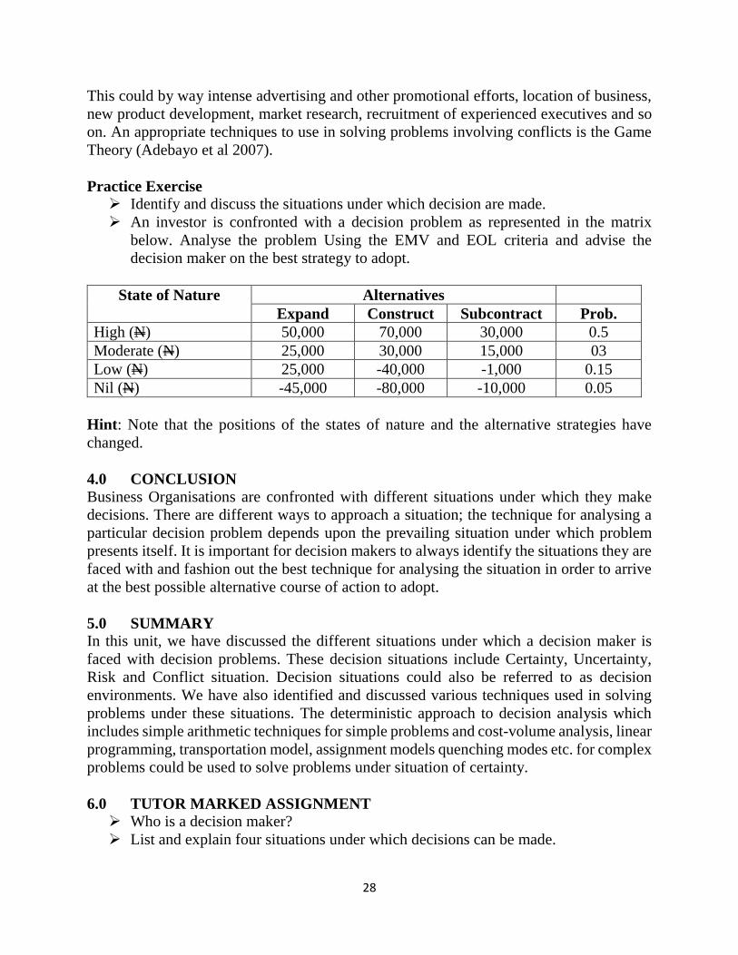
Practice Exercise

Identify and discuss the situations under which decision are made.

An investor is confronted with a decision problem as represented in the matrix

below. Analyse the problem Using the EMV and EOL criteria and advise the

decision maker on the best strategy to adopt.

State of Nature Alternatives

Expand Construct Subcontract Prob.

High (N) 50,000 70,000 30,000 0.5

Moderate (N) 25,000 30,000 15,000 03

Low (N) 25,000 -40,000 -1,000 0.15

Nil (N) -45,000 -80,000 -10,000 0.05

Hint: Note that the positions of the states of nature and the alternative strategies have

changed.

4.0 CONCLUSION

Business Organisations are confronted with different situations under which they make

decisions. There are different ways to approach a situation; the technique for analysing a

particular decision problem depends upon the prevailing situation under which problem

presents itself. It is important for decision makers to always identify the situations they are

faced with and fashion out the best technique for analysing the situation in order to arrive

at the best possible alternative course of action to adopt.

5.0 SUMMARY In this unit, we have discussed the different situations under which a decision maker is

faced with decision problems. These decision situations include Certainty, Uncertainty,

Risk and Conflict situation. Decision situations could also be referred to as decision

environments. We have also identified and discussed various techniques used in solving

problems under these situations. The deterministic approach to decision analysis which

includes simple arithmetic techniques for simple problems and cost-volume analysis, linear

programming, transportation model, assignment models quenching modes etc. for complex

problems could be used to solve problems under situation of certainty.


Who is a decision maker?

List and explain four situations under which decisions can be made.

29

Identify the techniques that can be used to analyse decision problems under the

following situations

(i) Certainty

(ii) Uncertainty

(iii) Risk

(iv) Conflict

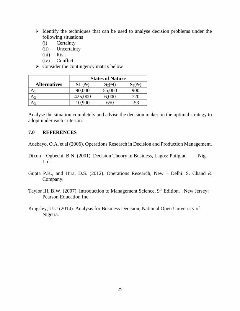
Consider the contingency matrix below

Alternatives

States of Nature

S1 (N) S2(N) S3(N)

A1 90,000 55,000 900

A2 425,000 6,000 720

A3 10,900 650 -53

Analyse the situation completely and advise the decision maker on the optimal strategy to

adopt under each criterion.

7.0 REFERENCES

Adebayo, O.A. et al (2006). Operations Research in Decision and Production Management.

Dixon – Ogbechi, B.N. (2001). Decision Theory in Business, Lagos: Philglad Nig.

Ltd.

Gupta P.K., and Hira, D.S. (2012). Operations Research, New – Delhi: S. Chand &

Company.

Taylor III, B.W. (2007). Introduction to Management Science, 9th Edition. New Jersey:

Pearson Education Inc.


Nigeria.

30

UNIT 3: DECISION TREES

1.0 Introduction

2.0 Objectives

3.0 Main Content

3.1 Definition

3.2 Benefits of using decision tree

3.3 Disadvantage of the decision tree

3.4 Components of the decision tree

3.5 Structure of a decision tree

3.6 How to analyse a decision tree

3.7 The Secretary Problem

3.7.1 Advantages of the Secretary Problem over the General Decision

tree

3.7.2 Analysis of the Secretary Problem

4.0 Conclusion

5.0 Summary


7.0 References

1.0 INTRODUCTION

So far, we have been discussing the techniques used for decision analysis. We have

demonstrated how to solve decision problems by presenting them in a tabular form.

However, if decision problems can be presented on a table, we can also represent the

problem graphically in what is known as a decision tree. Also the decision problems

discussed so far dealt with only single stage decision problem.

2.0 OBJECTIVES

After studying this unit, you should be able to;

Describe a decision tree

Describe what Decision nodes and outcome nodes are \

Represent problems in a decision trees and perform the fold back and tracing

forward analysis

Calculate the outcome values using the backward pass

Identify the optimal decision strategy

3.0 MAIN CONTENT

3.1 DEFINITION

A decision tree is a graphical representation of the decision process indicating decision

alternatives, states of nature, probabilities attached to the states of nature and conditional

benefits and losses (Gupta & Hira 2012). A decision tree is a pictorial method of showing

a sequence of inter-related decisions and outcomes. All the possible choices are shown on

the tree as branches and the possible outcomes as subsidiary branches. In summary, a

31

decision tree shows: the decision points, the outcomes (usually dependent on probabilities

and the outcomes values) (Lucey, 2001).

3.2 BENEFITS OF USING DECISION TREE

Dixon-Ogbechi (2001) presents the following advantages of using the decision tree

They assist in the clarification of complex decisions making situations that involve

risk.

Decision trees help in the quantification of situations.

Better basis for rational decision making are provided by decision trees.

They simplify the decision making process.

3.3 DISADVANTAGE OF THE DECISION TREE

The disadvantage of the decision tree is that it becomes time consuming, cumbersome and

difficult to use/draw when decision options/states of nature are many.

3.4 COMPONENTS OF THE DECISION TREE

It is important to note the following components of the structure of a decision problem

The choice or Decision Node: Basically, decision trees begin with choice or

decision nodes. The decision nodes are depicted by square . It is a point in the

decision tree were decisions would have to be made. Decision nodes are immediately

by alternative courses of action in what can be referred to as the decision fork. The

decision fork is depicted by a square with arrows or lines emanating from the

right side of the square .The number of lines emanating from the box depend

on the number of alternatives available.

Change Node: The chance node can also be referred to as state of nature node or event

node. Each node describes a situation in which an element of uncertainty is resolved. Each

way in this uncertainty can be resolved is represented by an arc that leads rightward from

its chance node, either to another node or to an end-point. The probability on each such arc

is a conditional probability, the condition being that one is at the chance node to its left.

These conditional probabilities sum to 1 (0ne), as they do in probability tree (Denardo,

2002).

The state of nature or chance nodes are depicted by circles it implies that at this

point, the decision maker will have to compute the expected monetary value (EMV)

of each state of nature. Again the chance event node is depicted this ( )

3.5 STRUCTURE OF A DECISION TREE

The structure and the typical components of a decision tree are shown in the diagram

below.

32

D

Action BOutcome X

1

Action B1

2Outcome X 2

Outcome X 3

D1

2

Outcome Y

Action

Action A 2

3Outcome Y 2

Action c1

Actionc2

Actionc3

D1

A1

Adapted from Lucey, T (2001), Quantitative Techniques, 5th London: Continuum.

The above is a typical construction of a decision tree. The decision tree begins with a

decision node D1 signifying that the decision maker is first of all presented with a decision

to make. Immediately after the decision node, there are two courses of Action A1 and A2.If

the decision maker chooses A1, there are three possible outcomes – X1 X2, X3. And if

chooses A2, there will be two possible outcomes Y1 and Y2 and so on.

3.6 HOW TO ANALYSE A DECISION TREE

The decision tree is a graphical representation of a decision problem. It is multi-state in

nature. As a result, a sequence of decisions are made repeatedly over a period of time and

such decisions depend on previous decisions and may lead to a set of probabilistic

outcomes. The decision tree analysis process is a form of probabilistic dynamic

programming (Dixon-Ogbechi, 2001).

Analysing a decision tree involves two states

i. Backward Pass: This involves the following steps

Starting from the right hand side of the decision tree, identify the nearest terminal.

If it is a chance event, calculate the EMV (Expected Monetary Value). And it is a

decision node, select the alternative that satisfies your objective.

33

Repeat the same operation in each of the terminals until you get to the end of the

left hand side of the decision tree.

ii. Forward Pass: The forward pass analysis involves the following operation.

Start from the beginning of the tree at the right hand side, at each point, select the

alternative with the largest value in the case of a minimization problem or profit

payoff, and the least payoff in the case of a minimization problem or cost payoff.

Trace forward the optimal contingency strategy by drawing another tree only with

the desired strategy.

These steps are illustrate below

EXAMPLE 4.1

Contingency Matrix 1

States of Nature

Alternatives

Probability

Stock Rice

(A1)

Stock Maize

(A2)

High demand

(S1) (N)

8,000 12,000 0.6

Low demand

(S2) (N)

4,000 -3,000 0.4

Fig. 4.1: Pay-off Matrix

Question: Represent the above payoff matrix on a decision tree and find the optimum

contingency strategy.

We can represent the above problem on a decision tree thus: S1(high demand) 8,000 0.6

A1(stock rice)S2(low demand)

0.4 4,000

S1(high demand) 12,000 A2(stock maize) 0.6 S2(high demand)

0.4-3,000

6400

6400

6000

34

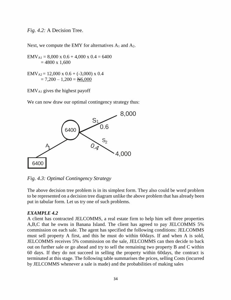
Fig. 4.2: A Decision Tree.

Next, we compute the EMY for alternatives A1 and A2.

EMVA1 = 8,000 x 0.6 + 4,000 x 0.4 = 6400

= 4800 x 1,600

EMVA2 = 12,000 x 0.6 + (-3,000) x 0.4

= 7,200 – 1,200 = N6,000

EMVA1 gives the highest payoff

We can now draw our optimal contingency strategy thus:

6400

S2

8,000

0.6

0.44,000

S1

A1

6400

Fig. 4.3: Optimal Contingency Strategy

The above decision tree problem is in its simplest form. They also could be word problem

to be represented on a decision tree diagram unlike the above problem that has already been

put in tabular form. Let us try one of such problems.

EXAMPLE 4.2

A client has contracted JELCOMMS, a real estate firm to help him sell three properties

A,B,C that he owns in Banana Island. The client has agreed to pay JELCOMMS 5%

commission on each sale. The agent has specified the following conditions: JELCOMMS

must sell property A first, and this he must do within 60days. If and when A is sold,

JELCOMMS receives 5% commission on the sale, JELCOMMS can then decide to back

out on further sale or go ahead and try to sell the remaining two property B and C within

60 days. If they do not succeed in selling the property within 60days, the contract is

terminated at this stage. The following table summarises the prices, selling Costs (incurred

by JELCOMMS whenever a sale is made) and the probabilities of making sales

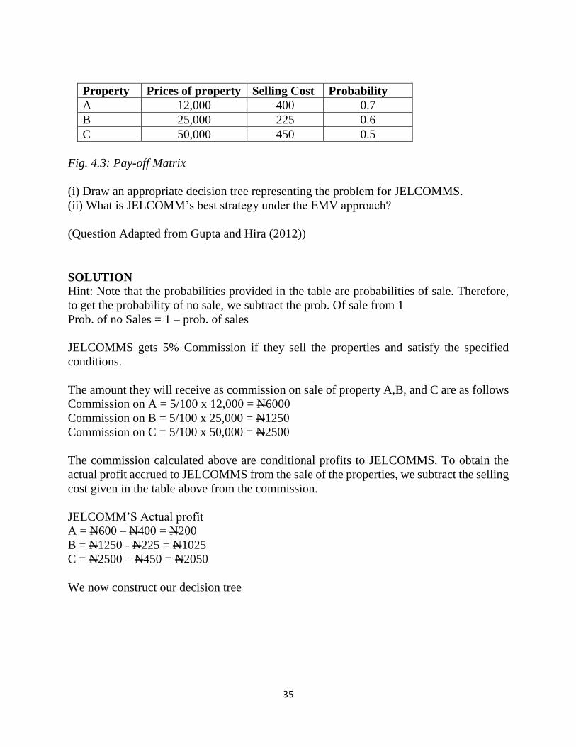
35

Property Prices of property Selling Cost Probability

A 12,000 400 0.7

B 25,000 225 0.6

C 50,000 450 0.5

Fig. 4.3: Pay-off Matrix

(i) Draw an appropriate decision tree representing the problem for JELCOMMS.

(ii) What is JELCOMM’s best strategy under the EMV approach?

(Question Adapted from Gupta and Hira (2012))

SOLUTION

Hint: Note that the probabilities provided in the table are probabilities of sale. Therefore,

to get the probability of no sale, we subtract the prob. Of sale from 1

Prob. of no Sales = 1 – prob. of sales

JELCOMMS gets 5% Commission if they sell the properties and satisfy the specified

conditions.

The amount they will receive as commission on sale of property A,B, and C are as follows

Commission on A = 5/100 x 12,000 = N6000

Commission on B = 5/100 x 25,000 = N1250

Commission on C = 5/100 x 50,000 = N2500

The commission calculated above are conditional profits to JELCOMMS. To obtain the

actual profit accrued to JELCOMMS from the sale of the properties, we subtract the selling

cost given in the table above from the commission.

JELCOMM’S Actual profit

A = N600 – N400 = N200

B = N1250 - N225 = N1025

C = N2500 – N450 = N2050

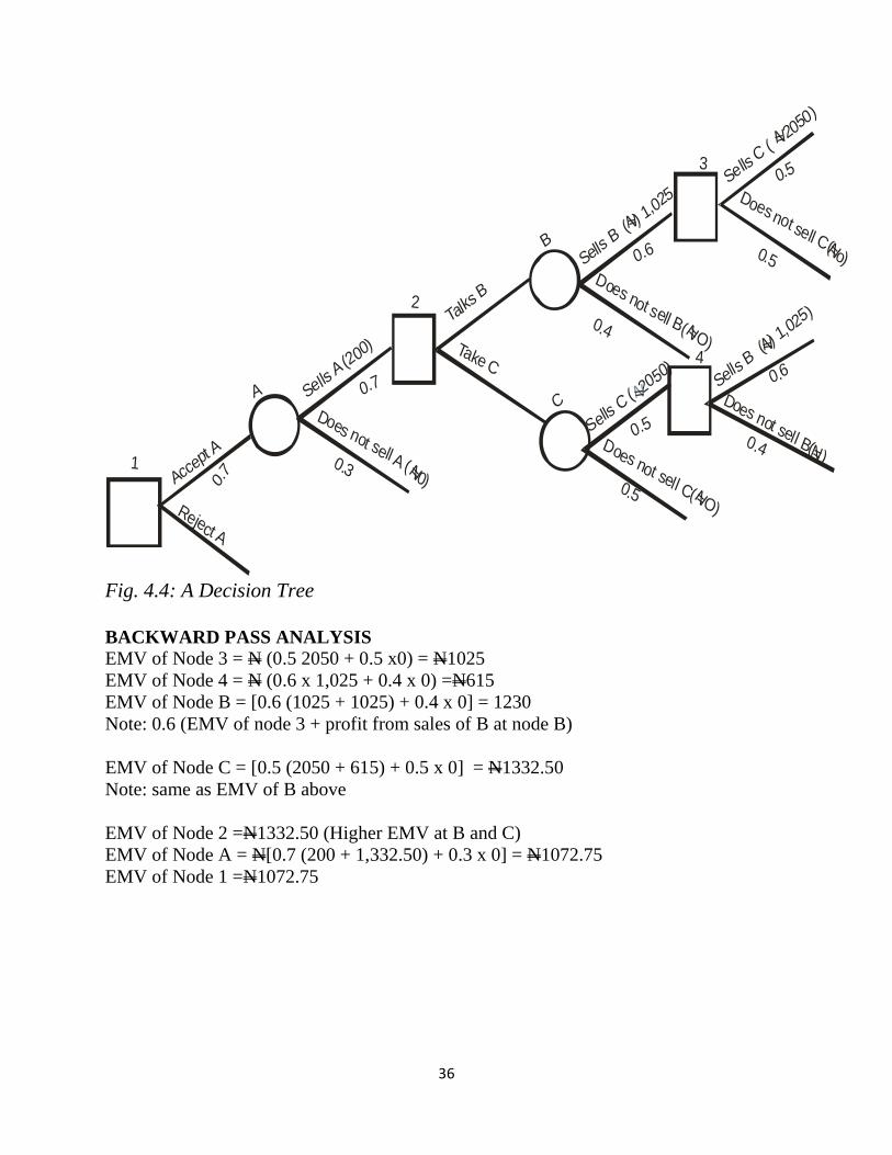
We now construct our decision tree

36

Accep

t A

Reject A

1

Sells A (2

00)

Does not sell A ( 0)

N

0.3

A

2Ta

lks B

Take C

BSell

s B (

) 1,02

5Sells

C ( 2

050)

N

Does not sell C(N o)

0.4

0.7 N

0.7

0.5 Does not sell B(N O)

Sells C

( 20

50)

N

0.5 Does not sell C(N O)

3

Sells B

( )

1,025

)

N

Does not sell B(N)

0.5

0.4

4

C

0.5

0.6

0.6

Fig. 4.4: A Decision Tree

BACKWARD PASS ANALYSIS

EMV of Node 3 = N (0.5 2050 + 0.5 x0) = N1025

EMV of Node 4 = N (0.6 x 1,025 + 0.4 x 0) =N615

EMV of Node B = [0.6 (1025 + 1025) + 0.4 x 0] = 1230

Note: 0.6 (EMV of node 3 + profit from sales of B at node B)

EMV of Node C = [0.5 (2050 + 615) + 0.5 x 0] = N1332.50

Note: same as EMV of B above

EMV of Node 2 =N1332.50 (Higher EMV at B and C)

EMV of Node A = N[0.7 (200 + 1,332.50) + 0.3 x 0] = N1072.75

EMV of Node 1 =N1072.75

37

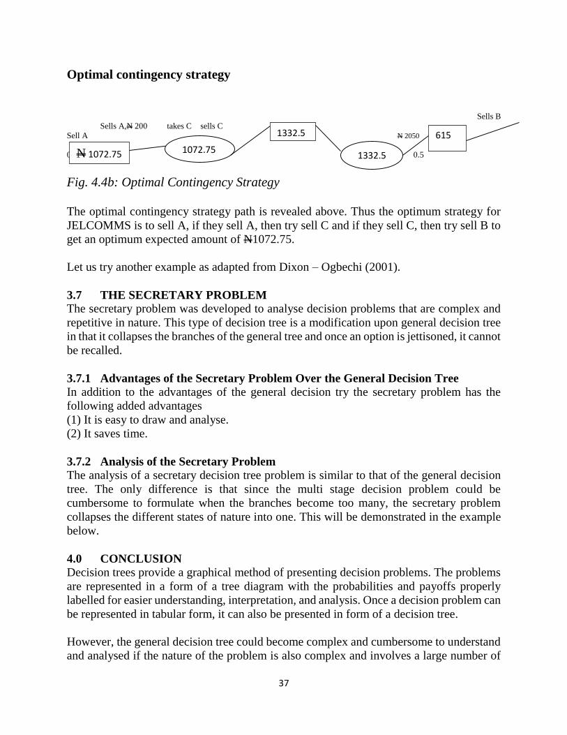
Optimal contingency strategy

Sells B

Sells A,N 200 takes C sells C N1025

Sell A N 2050

0.7 0.5

Fig. 4.4b: Optimal Contingency Strategy

The optimal contingency strategy path is revealed above. Thus the optimum strategy for

JELCOMMS is to sell A, if they sell A, then try sell C and if they sell C, then try sell B to

get an optimum expected amount of N1072.75.

Let us try another example as adapted from Dixon – Ogbechi (2001).

3.7 THE SECRETARY PROBLEM

The secretary problem was developed to analyse decision problems that are complex and

repetitive in nature. This type of decision tree is a modification upon general decision tree

in that it collapses the branches of the general tree and once an option is jettisoned, it cannot

be recalled.

3.7.1 Advantages of the Secretary Problem Over the General Decision Tree

In addition to the advantages of the general decision try the secretary problem has the

following added advantages

(1) It is easy to draw and analyse.

(2) It saves time.

3.7.2 Analysis of the Secretary Problem

The analysis of a secretary decision tree problem is similar to that of the general decision

tree. The only difference is that since the multi stage decision problem could be

cumbersome to formulate when the branches become too many, the secretary problem

collapses the different states of nature into one. This will be demonstrated in the example

below.

4.0 CONCLUSION

Decision trees provide a graphical method of presenting decision problems. The problems

are represented in a form of a tree diagram with the probabilities and payoffs properly

labelled for easier understanding, interpretation, and analysis. Once a decision problem can

be represented in tabular form, it can also be presented in form of a decision tree.

However, the general decision tree could become complex and cumbersome to understand

and analysed if the nature of the problem is also complex and involves a large number of

1332.5 N 1072.75 1072.75

1332.5 615

38

options. The secretary formulation method of the general decision tree was developed as

an improvement upon the general formulation to be used for analysing complex and

cumbersome decision problems. Generally, the decision tree provides a simple and straight

forward way of analysing decision problems.

5.0 SUMMARY

Now let us cast our minds back to what we have learnt so far in this unit. We learnt that

the decision tree is mostly used for analysing a multi-stage decision problem. That is, when

there is a sequence of decisions to be made with each decision having influence on the

next. A decision tree is a pictorial method of showing a sequence of inter-related decisions

and outcomes. It is a graphical representation that outlines the different states of nature,

alternatives courses of actions with their corresponding probabilities. The branches of a

decision tree are made up of the decision nodes at which point a decision is to be made,

and the chance node at which point the EMV is to be computed.


What do you understand by the term decision tree?

Identify the two formulations of the decision tree and give the difference between

them.

Outline the advantages and disadvantage of a decision tree.

Write short notes on the following:

i Decision Node

ii Chance Even Node

Identify and discuss the two method of analysis of a decision tree

7.0 REFERENCES


Ltd.

Denardo, E.V. (2002). The Schience of Decision making: A Problem-Based Approach

Using Excel. New York: John Wiley.

Gupta, P.K., and Hira, D.S. (2012). Operations Research, New – Delhi: S. Chand &

Company.


Nigeria.

39

UNIT 4: OPERATIONAL RESEARCH APPROACHES TO DECISION

ANALYSIS

1.0 Introduction

2.0 Objectives

3.0 Main Content

3.1 Main Approaches to Decision Analysis

3.1.1 Qualitative Approach to Decision Making

3.1.2 Quantitative Approach

3.2 Objective of Decision Making

3.3 Steps in Decision Theory Approach

3.4 Decision Making Criteria

3.4.1 Maximax Criterion (Criterion of Optimism)

3.4.2 Maximin Criterion (Criterion of Pessimism)

3.4.3 Minimax Regret Criterion (Savage Criterion)

3.4.4 Equally Likely of Laplace Criterion (Bayes’ or Criterion of

Rationality

3.4.5 Hurwicz Criterion (Criterion of Realism)

4.0 Conclusion

5.0 Summary


7.0 References

1.0 INTRODUCTION

We discussed what the subject Decision Analysis is all about we defined a decision,

decision maker, business decision analysis and threw light on various components involved

in Business Decision Analysis. In this unit, we shall proceed to explaining the different

approaches used in analysing a decision problem. Two key approaches present themselves

– Qualitative Approach, and the Quantitative Approach. These two broad approaches from

the core of business decision analysis. They will be broken down into several specific

methods that will be discussed throughout in this course of study.

2.0 OBJECTIVES

After studying this unit, you should be able to:

Identify the qualitative and quantitative approaches to decision analysis.

Identify the qualitative and quantitative tools of analysis.

Use the Expected monetary value (EMV) and Expected opportunity (EOL)

techniques in solving decision problems.

Solve decision problems using the different criteria available.

40

2.0 MAIN CONTENT

3.1 MAIN APPROACHES TO DECISION ANALYSIS As identified earlier, the two main approaches to decision analysis are the qualitative and

quantitative approaches.

3.1.1 QUALITATIVE APPROACH TO DECISION MAKING

Qualitative approaches to decision analysis are techniques that use human judgement and

experience to turn qualitative information into quantitative estimates (Lucey 1988) as

quoted by Dixon – Ogbechi (2001). He identified the following qualitative decision

techniques

Delphi Method

Market Research

Historical Analogy

According to Akingbade (1995), qualitative models are often all that are feasible to use in

circumstances, and such models can provide a great deal of insight and enhance the quality

of decisions that can be made. Quantitative models inform the decision maker about

relationships among kinds of things.Knowledge of such relationships can inform the

decision maker about areas to concentrate upon so as to yield desired results.

Akingbade (1995) presented the following examples of qualitative models:

Influence diagrams.

Cognitive maps.

Black box models.

Venn Diagrams.

Decision trees.

Flow charts etc.

(Dixon – Ogbechi 2001)

Let us now consider the different qualitative approaches to decision making.

Delphi Method: The Delphi method is technique that is designed to obtain expert

consensus for a particular forecast without the problem of submitting to pressure to

conform to a majority view. It is used for long term forecasting. Under this method, a panel

is made to independently answer a sequence of questionnaire which is used to produce the

next questionnaire. As a result, any information available to a group of experts is passed

on to all, so that subsequent judgements are refined as more information and experience

become available (Lucey 1988).

Market Research: These are widely used procedures involving opinion surveys; analysis

of market data, questionnaires designed to gage the reaction of the market to a particular

product, design, price, etc. It is often very accurate for a relatively short term.

41

Historical Analogy: Historical Analogy is used where past data on a particular item are

not available. In such cases, data on similar subjects are analysed to establish the life cycle

and expected sales of the new product. This technique is useful in forming a board

impression in the medium to long term. (Lucey (1988) as quoted by Dixon-Ogbechi

(2001)).

3.1.2 QUANTITATIVE APPROACH

This technique or approach lends itself to the careful measurement of operational

requirements and returns. This makes the task of comparing one alternative with another

very much more objective. Quantitative technique as argued by Dixon-Ogbechi (2001),

embraces all the operational techniques that lend themselves to quantitative measurement.

Harper (1975) presents the following quantitative techniques.

(a) Mathematics: Skemp (1971) defined Mathematics as “a system of abstraction,

classification and logical reasoning. Generally, Mathematics can be subdivided into

two

i. Pure Mathematics

ii. Applied Mathematics

i. Pure Mathematics is absolutely abstract in not concerning itself with anything concrete

but purely with structures and logical applications, implications and consequences of such

structures.

ii. Applied Mathematics is the application of proved abstract generalization (from pure

Mathematics) to the physical world (Akingbade, 1996) both pure and applied Mathematics

can be broken into the following subdivisions.

(1) Arithmetic

(2) Geometry

(3) Calculus

(4) Algebra

(5) Trigonometry

(6) Statistics

(b) Probability: Probability is widely used in analysing business decisions, Akingbade

(1996) defined probability as a theory concerned with the study of processes

involving uncertainty. Lucey (1988) defined probability as “the quantification of

uncertainty”. Uncertainty may be expressed as likelihood, chance or risk.

(c) Mathematical Models: According to Dixon-Ogbechi (2001), A Mathematical

model is a simplified representation of a real life situation in Mathematical terms.

A Mathematical model is Mathematical idealization in the form of a system

proposition, formula or equation of a physical, biological or social phenomenon

(Encarta Premium, 2009).

42

(d) Statistics: Statistics has been described as a branch of Mathematics that deals with

the collection, organization, and analysis of numerical data and with such problems

as experiment design and decision making (Microsoft Encarta Premium, 2009).

3.2 OBJECTIVE OF DECISION MAKING Before a decision maker embarks on the process of decision making he/she must set clear

objectives as to what is expected to be achieved at the end of the process. In Business

decision analysis; there are two broad objectives that decision makers can possible set to

achieve. These are:

Maximization of profit, and

Minimization of Loss

Most decisions in business fall under these two broad categories of objectives. The decision

criterion to adopt will depend on the objective one is trying to achieve.

In order to achieve profit maximization, the Expected Monetary Value (EMV) approach is

most appropriate. As will be seen later, the Expected Value of the decision alternative is

the sum of highlighted pay offs for the decision alternative, with the weight representing

the probability of occurrence of the states of nature. This approach is possible when there

are probabilities attached to each state of nature or event. The EMV approach to decision

making is assumed to be used by the optimistic decision maker who expects to maximize

profit from his investment. The technique most suitable for minimization of loss is the

Expected opportunity loss (EOL) approach. It is used in the situation where the decision

maker expects to make a loss from an investment and tries to keep the loss as minimum as

possible. This type of problem is known as minimization problem and the decision maker

here is known to be pessimistic. The problem under the EMV approach is known as a

maximization problem as the decision maker seeks to make the most profit from the

investment. These two approaches will be illustrated in details in the next section.

3.3 STEPS IN DECISION THEORY APPROACH

Decision theory approach generally involves four steps. Gupta and Hira (2012) present the

following four steps.

Step 1: List all the viable alternatives

The first action the decision maker must take is to list all viable alternatives that can be

considered in the decision. Let us assume that the decision maker has three alternative

courses of action available to him a, b, c.

Step 2: Identify the expected future event

The second step is for the decision maker to identify and list all future occurrences. Often,

it is possible for the decision maker to identify the future states of nature; the difficulty is

43

to identify which one will occur. Recall, that these future states of nature or occurrences

are not under the control of the decision maker. Let us assume that the decision maker has

identified four of these states of nature: i, ii, iii, iv.

Step 3: Construct a payoff table

After the alternatives and the states of nature have been identified, the next task is for the

decision maker to construct a payoff table for each possible combination of alternative

courses of action and states of nature. The payoff table can also be called contingency table.

Step 4: Select optimum decision criterion

Finally, the decision maker will choose a criterion which will result in the largest payoff

or which will maximize his wellbeing or meet his objective. An example of pay off table

is presented below.

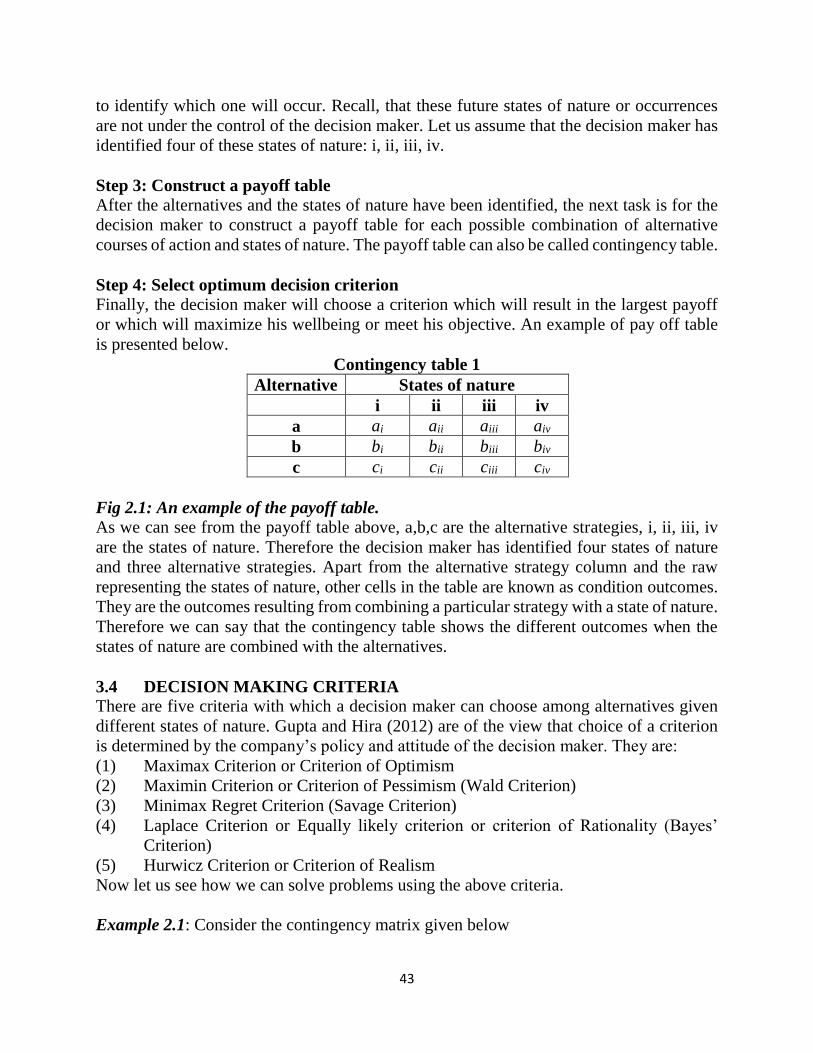
Contingency table 1

Alternative States of nature

i ii iii iv

a ai aii aiii aiv

b bi bii biii biv

c ci cii ciii civ

Fig 2.1: An example of the payoff table.

As we can see from the payoff table above, a,b,c are the alternative strategies, i, ii, iii, iv

are the states of nature. Therefore the decision maker has identified four states of nature

and three alternative strategies. Apart from the alternative strategy column and the raw

representing the states of nature, other cells in the table are known as condition outcomes.

They are the outcomes resulting from combining a particular strategy with a state of nature.

Therefore we can say that the contingency table shows the different outcomes when the

states of nature are combined with the alternatives.

3.4 DECISION MAKING CRITERIA

There are five criteria with which a decision maker can choose among alternatives given

different states of nature. Gupta and Hira (2012) are of the view that choice of a criterion

is determined by the company’s policy and attitude of the decision maker. They are:

(1) Maximax Criterion or Criterion of Optimism

(2) Maximin Criterion or Criterion of Pessimism (Wald Criterion)

(3) Minimax Regret Criterion (Savage Criterion)

(4) Laplace Criterion or Equally likely criterion or criterion of Rationality (Bayes’

Criterion)

(5) Hurwicz Criterion or Criterion of Realism

Now let us see how we can solve problems using the above criteria.

Example 2.1: Consider the contingency matrix given below

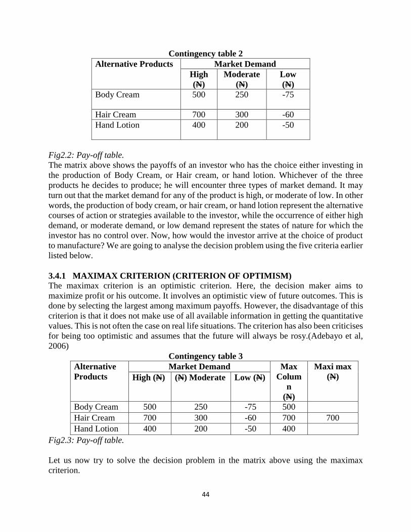
44

Contingency table 2

Alternative Products Market Demand

High

(N)

Moderate

(N)

Low

(N)

Body Cream 500 250 -75

Hair Cream 700 300 -60

Hand Lotion 400 200 -50

Fig2.2: Pay-off table.

The matrix above shows the payoffs of an investor who has the choice either investing in

the production of Body Cream, or Hair cream, or hand lotion. Whichever of the three

products he decides to produce; he will encounter three types of market demand. It may

turn out that the market demand for any of the product is high, or moderate of low. In other

words, the production of body cream, or hair cream, or hand lotion represent the alternative

courses of action or strategies available to the investor, while the occurrence of either high

demand, or moderate demand, or low demand represent the states of nature for which the

investor has no control over. Now, how would the investor arrive at the choice of product

to manufacture? We are going to analyse the decision problem using the five criteria earlier

listed below.

3.4.1 MAXIMAX CRITERION (CRITERION OF OPTIMISM)

The maximax criterion is an optimistic criterion. Here, the decision maker aims to

maximize profit or his outcome. It involves an optimistic view of future outcomes. This is

done by selecting the largest among maximum payoffs. However, the disadvantage of this

criterion is that it does not make use of all available information in getting the quantitative

values. This is not often the case on real life situations. The criterion has also been criticises

for being too optimistic and assumes that the future will always be rosy.(Adebayo et al,

2006)

Contingency table 3

Alternative

Products

Market Demand Max

Colum

n

(N)

Maxi max

(N) High (N) (N) Moderate Low (N)

Body Cream 500 250 -75 500

Hair Cream 700 300 -60 700 700

Hand Lotion 400 200 -50 400

Fig2.3: Pay-off table.

Let us now try to solve the decision problem in the matrix above using the maximax

criterion.

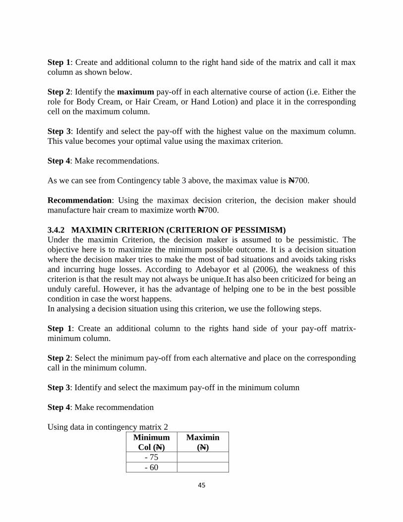
45

Step 1: Create and additional column to the right hand side of the matrix and call it max

column as shown below.

Step 2: Identify the maximum pay-off in each alternative course of action (i.e. Either the

role for Body Cream, or Hair Cream, or Hand Lotion) and place it in the corresponding

cell on the maximum column.

Step 3: Identify and select the pay-off with the highest value on the maximum column.

This value becomes your optimal value using the maximax criterion.

Step 4: Make recommendations.

As we can see from Contingency table 3 above, the maximax value is N700.

Recommendation: Using the maximax decision criterion, the decision maker should

manufacture hair cream to maximize worth N700.

3.4.2 MAXIMIN CRITERION (CRITERION OF PESSIMISM)

Under the maximin Criterion, the decision maker is assumed to be pessimistic. The

objective here is to maximize the minimum possible outcome. It is a decision situation

where the decision maker tries to make the most of bad situations and avoids taking risks

and incurring huge losses. According to Adebayor et al (2006), the weakness of this

criterion is that the result may not always be unique.It has also been criticized for being an

unduly careful. However, it has the advantage of helping one to be in the best possible

condition in case the worst happens.

In analysing a decision situation using this criterion, we use the following steps.

Step 1: Create an additional column to the rights hand side of your pay-off matrix-

minimum column.

Step 2: Select the minimum pay-off from each alternative and place on the corresponding

call in the minimum column.

Step 3: Identify and select the maximum pay-off in the minimum column

Step 4: Make recommendation

Using data in contingency matrix 2

Minimum

Col (N)

Maximin

(N)

- 75

- 60

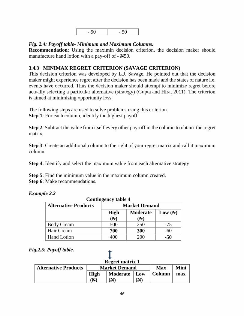
46

- 50 - 50

Fig. 2.4: Payoff table- Minimum and Maximum Columns.

Recommendation: Using the maximin decision criterion, the decision maker should

manufacture hand lotion with a pay-off of - N50.

3.4.3 MINIMAX REGRET CRITERION (SAVAGE CRITERION)

This decision criterion was developed by L.J. Savage. He pointed out that the decision

maker might experience regret after the decision has been made and the states of nature i.e.

events have occurred. Thus the decision maker should attempt to minimize regret before

actually selecting a particular alternative (strategy) (Gupta and Hira, 2011). The criterion

is aimed at minimizing opportunity loss.

The following steps are used to solve problems using this criterion.

Step 1: For each column, identify the highest payoff

Step 2: Subtract the value from itself every other pay-off in the column to obtain the regret

matrix.

Step 3: Create an additional column to the right of your regret matrix and call it maximum

column.

Step 4: Identify and select the maximum value from each alternative strategy

Step 5: Find the minimum value in the maximum column created.

Step 6: Make recommendations.

Example 2.2

Contingency table 4

Alternative Products Market Demand

High

(N)

Moderate

(N)

Low (N)

Body Cream 500 250 -75

Hair Cream 700 300 -60

Hand Lotion 400 200 -50

Fig.2.5: Payoff table.

Regret matrix 1

Alternative Products Market Demand Max

Column

Mini

max High

(N)

Moderate

(N)

Low

(N)

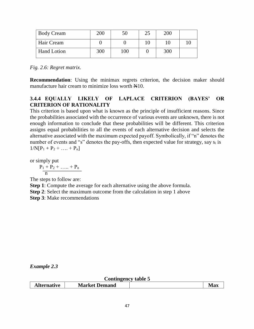
47

Body Cream 200 50 25 200

Hair Cream 0 0 10 10 10

Hand Lotion 300 100 0 300

Fig. 2.6: Regret matrix.

Recommendation: Using the minimax regrets criterion, the decision maker should

manufacture hair cream to minimize loss worth N10.

3.4.4 EQUALLY LIKELY OF LAPLACE CRITERION (BAYES’ OR

CRITERION OF RATIONALITY

This criterion is based upon what is known as the principle of insufficient reasons. Since

the probabilities associated with the occurrence of various events are unknown, there is not

enough information to conclude that these probabilities will be different. This criterion

assigns equal probabilities to all the events of each alternative decision and selects the

alternative associated with the maximum expected payoff. Symbolically, if “n” denotes the

number of events and “s” denotes the pay-offs, then expected value for strategy, say si is

1/N[P1 + P2 + …. + Pn]

or simply put

P1 + P2 + ….. + Pn

n

The steps to follow are:

Step 1: Compute the average for each alternative using the above formula.

Step 2: Select the maximum outcome from the calculation in step 1 above

Step 3: Make recommendations

Example 2.3

Contingency table 5

Alternative Market Demand Max

48

Products High

(N)

Moderate

(N)

Low

(N)

Average Column Col.

Body Cream 500 250 -75 500 +250 + 75 = 675

3 3 = 225

Hair Cream 700 300 -60 700 + 300 – 60 = 940

3 3 =313.3

313.3

Hand Lotion 400 200 -50 400 + 200 – 5 = 550

30 3 =183.3

Fig. 2.7: Payoff table.

Recommendation: Using the equally likely criterion, the decision should manufacture

Hair Cream worth N313.3

3.4.5 HURWICZ CRITERION (CRITERION OF REALISM)

This criterion is also called weighted average criterion. It is a compromise between the

maximax (optimistic) and maximin (Pessimistic) decision criteria. This concept allows the

decision maker to take into account both maximum and minimum for each alternative and

assign them weights according to his degree of optimism or pessimism. The alternative

which maximises the sum of these weighted pay-offs is then selected. (Gupta and Hira,

2012)

The Hurwicz Criterion Comsprises the following steps:

Step 1: Choose an appropriate degree of optimism ( lies between zero and one (0

<<1)), so that (1-) represents the degree of pessimism. is called coefficient or index

of optimism.

Step 2: Determine the maximum as well as minimum value of each alternative course of

action.

Step 3: Determine the criterion of realism using the following formula

CRi = (Max in Rowi) + (1 - ) (Min in Rowi)

Step 4: Select the maximum outcome in step 3 above

Step 5: Make Recommendation

Example 2.4

EXAMPLE: Using the contingency table 3 above,

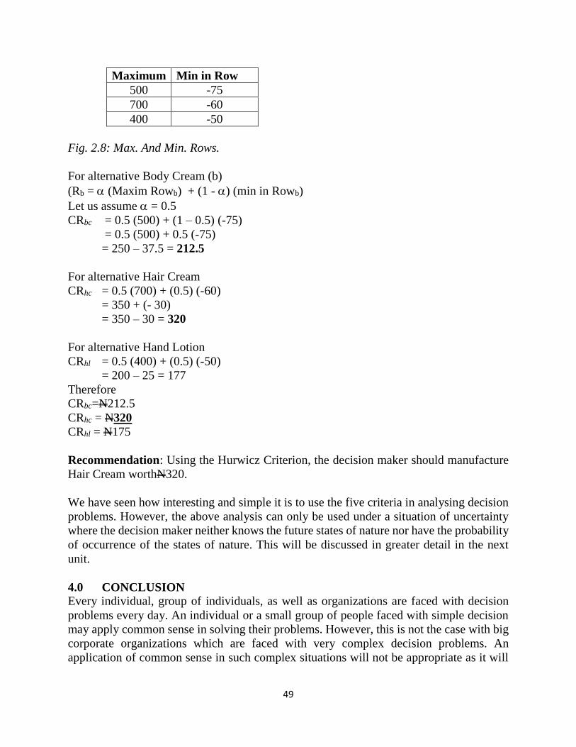
49

Maximum Min in Row

500 -75

700 -60

400 -50

Fig. 2.8: Max. And Min. Rows.

For alternative Body Cream (b)

(Rb = (Maxim Rowb) + (1 - ) (min in Rowb)

Let us assume = 0.5

CRbc = 0.5 (500) + (1 – 0.5) (-75)

= 0.5 (500) + 0.5 (-75)

= 250 – 37.5 = 212.5

For alternative Hair Cream

CRhc = 0.5 (700) + (0.5) (-60)

= 350 + (- 30)

= 350 – 30 = 320

For alternative Hand Lotion

CRhl = 0.5 (400) + (0.5) (-50)

= 200 – 25 = 177

Therefore

CRbc=N212.5

CRhc = N320

CRhl = N175

Recommendation: Using the Hurwicz Criterion, the decision maker should manufacture

Hair Cream worthN320.

We have seen how interesting and simple it is to use the five criteria in analysing decision

problems. However, the above analysis can only be used under a situation of uncertainty

where the decision maker neither knows the future states of nature nor have the probability

of occurrence of the states of nature. This will be discussed in greater detail in the next

unit.

4.0 CONCLUSION

Every individual, group of individuals, as well as organizations are faced with decision

problems every day. An individual or a small group of people faced with simple decision

may apply common sense in solving their problems. However, this is not the case with big

corporate organizations which are faced with very complex decision problems. An

application of common sense in such complex situations will not be appropriate as it will

50

lead mostly to wrong decisions. Complex decision problems demand the use of specialized

tools and techniques for analysis of problem and eventual arrival at the best alternative.

5.0 SUMMARY This unit outlines briefly some approaches to decision analysis. It identifies two basic

approaches to decision analysis: Qualitative and Quantitative approaches. The Qualitative

approach includes: Delphi Method, Market Research and Historical Analogy. The

Quantitative technique includes the use of Mathematics, Probability, Mathematical models

and statistics to analyse decision problems. Finally, we discuss the five criteria for solving

problems under the condition of uncertainty: maximax, maximin, laplace’s, minimax

regret, and Hurwicz criterion.

6.0 TUTOR MARKET ASSIGNMENT

Differential between qualitative and quantitative techniques.

List and explain four qualitative techniques of decision analysis.

What do your understanding by a state of Nature?

Differentials between the Expected monetary value (EMV) and the Expected

opportunity Loss (EOL) techniques.

Consider the payoff matrix below and analyse the decision problem completely.

Contingency table 6

Alternatives

State of nature

S1 S2 S3

d1 15,000 35,000 200

d2 75,000 15,000 -100

d3 20,000 45,000 -1,000

Hint: Whenever you are asked to analyse a problem completely, it means you should use

the five criteria early discussed for analyse the decision problem.

7.0 REFERENCE Adebayo, O.A. et al (2006). Operations Research in Decision and Production Management.

Akingbade, F. (1995). Practical Operational Research for Developing Countries: A

Process Framework approach, Lagos: Panaf Publishing Inc.


Ltd.

Gupta, P.K and Hira, D.S. (2012). Operations Research, New – Delhi: S. Chand &

Company.

51

Harper, W.M. (1975). Operational Research, London: Macdonald & Evans Ltd.

Lucey, T. (1988). Quantitative Techniques: An Instructional Manual, London: DP

Publications.


Nigeria.

MODULE TWO

UNIT 5: SYSTEMS AND SYSTEM ANALYSIS

1.0 Introduction

2.0 Objectives

52

3.0 Main content

3.1 Definition

3.2 The Systems Theory

3.3 Elements of a System

3.4 Types of Systems

3.5 Forms of Systems

3.5.1 Conceptual System

3.5.2 Mechanical System

3.5.3 Social System

3.5.4 Deterministic System

3.5.5 Probabilistic System

3.6 The Concept of Entropy in a System

4.0 Conclusion

5.0 Summary


7.0 References

1.0 INTRODUCTION

The word system has a long history which can be traced back to Plato (Philebus), Aristotle

(Politics) and Euclid (Elements). It had meant "total", "crowd" or "union" in even more

ancient times, as it derives from the verb sunìstemi, uniting, putting together.

"System" means "something to look at". You must have a very high visual gradient to have

systematization. In philosophy, before Descartes, there was no "system". Plato had no

"system". Aristotle had no "system"(McLuhan. 1967)

In the 19th century the first to develop the concept of a "system" in the natural sciences

was the French physicist Nicolas Léonard Sadi Carnot who studied thermodynamics. In

1824 he studied the system which he called the working substance, i.e. typically a body of

water vapour, in steam engines, in regards to the system's ability to do work when heat is

applied to it. The working substance could be put in contact with either a boiler, a cold

reservoir (a stream of cold water), or a piston (to which the working body could do work

by pushing on it). In 1850, the German physicist Rudolf Clausius generalized this picture

to include the concept of the surroundings and began to use the term "working body" when

referring to the system.

2.0 OBJECTIVES

After studying this unit, you should be able to

Define a system

Identify and describe the types of systems

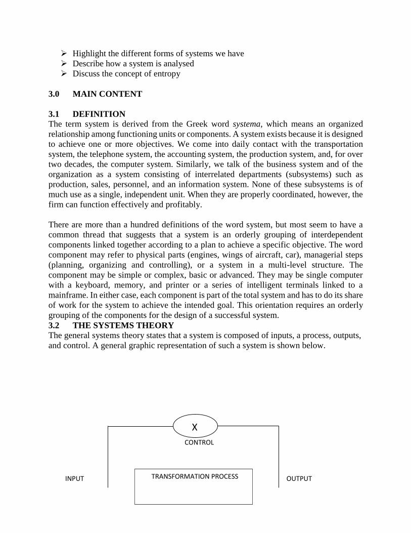
53

Highlight the different forms of systems we have

Describe how a system is analysed

Discuss the concept of entropy

3.0 MAIN CONTENT

3.1 DEFINITION

The term system is derived from the Greek word systema, which means an organized

relationship among functioning units or components. A system exists because it is designed

to achieve one or more objectives. We come into daily contact with the transportation

system, the telephone system, the accounting system, the production system, and, for over

two decades, the computer system. Similarly, we talk of the business system and of the

organization as a system consisting of interrelated departments (subsystems) such as

production, sales, personnel, and an information system. None of these subsystems is of

much use as a single, independent unit. When they are properly coordinated, however, the

firm can function effectively and profitably.

There are more than a hundred definitions of the word system, but most seem to have a

common thread that suggests that a system is an orderly grouping of interdependent

components linked together according to a plan to achieve a specific objective. The word

component may refer to physical parts (engines, wings of aircraft, car), managerial steps

(planning, organizing and controlling), or a system in a multi-level structure. The

component may be simple or complex, basic or advanced. They may be single computer

with a keyboard, memory, and printer or a series of intelligent terminals linked to a

mainframe. In either case, each component is part of the total system and has to do its share

of work for the system to achieve the intended goal. This orientation requires an orderly

grouping of the components for the design of a successful system.

3.2 THE SYSTEMS THEORY The general systems theory states that a system is composed of inputs, a process, outputs,

and control. A general graphic representation of such a system is shown below.

CONTROL INPUT OUTPUT TRANSFORMATION PROCESS

X

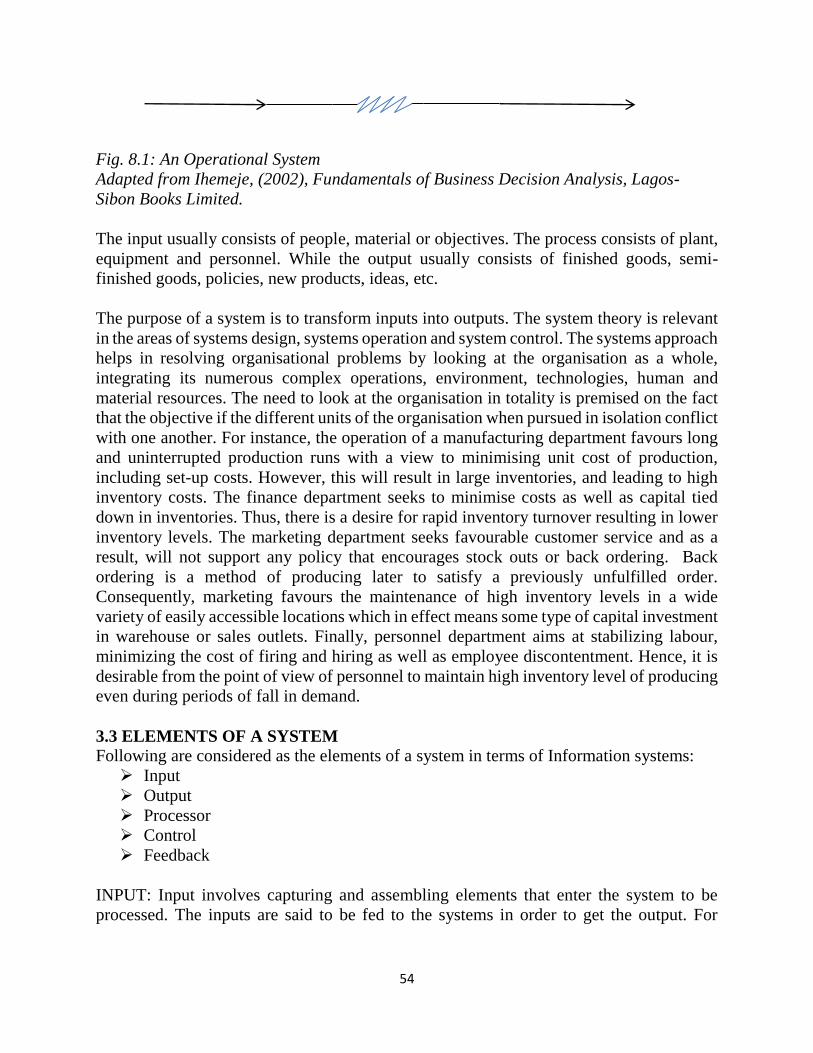
54

Fig. 8.1: An Operational System

Adapted from Ihemeje, (2002), Fundamentals of Business Decision Analysis, Lagos-

Sibon Books Limited.

The input usually consists of people, material or objectives. The process consists of plant,

equipment and personnel. While the output usually consists of finished goods, semi-

finished goods, policies, new products, ideas, etc.

The purpose of a system is to transform inputs into outputs. The system theory is relevant

in the areas of systems design, systems operation and system control. The systems approach

helps in resolving organisational problems by looking at the organisation as a whole,

integrating its numerous complex operations, environment, technologies, human and

material resources. The need to look at the organisation in totality is premised on the fact

that the objective if the different units of the organisation when pursued in isolation conflict

with one another. For instance, the operation of a manufacturing department favours long

and uninterrupted production runs with a view to minimising unit cost of production,

including set-up costs. However, this will result in large inventories, and leading to high

inventory costs. The finance department seeks to minimise costs as well as capital tied

down in inventories. Thus, there is a desire for rapid inventory turnover resulting in lower

inventory levels. The marketing department seeks favourable customer service and as a

result, will not support any policy that encourages stock outs or back ordering. Back

ordering is a method of producing later to satisfy a previously unfulfilled order.

Consequently, marketing favours the maintenance of high inventory levels in a wide

variety of easily accessible locations which in effect means some type of capital investment

in warehouse or sales outlets. Finally, personnel department aims at stabilizing labour,

minimizing the cost of firing and hiring as well as employee discontentment. Hence, it is

desirable from the point of view of personnel to maintain high inventory level of producing

even during periods of fall in demand.

3.3 ELEMENTS OF A SYSTEM

Following are considered as the elements of a system in terms of Information systems:

Input

Output

Processor

Control

Feedback

INPUT: Input involves capturing and assembling elements that enter the system to be

processed. The inputs are said to be fed to the systems in order to get the output. For

55

example, input of a 'computer system' is input unit consisting of various input devices like

keyboard, mouse, joystick etc.

OUTPUT: The element that exists in the system due to the processing of the inputs is

known as output. A major objective of a system is to produce output that has value to its

user. The output of the system maybe in the form of cash, information, knowledge, reports,

documents etc. The system is defined as output is required from it. It is the anticipatory

recognition of output that helps in defining the input of the system. For example, output of

a 'computer system' is output unit consisting of various output devices like screen and

printer etc.

PROCESSOR(S): The processor is the element of a system that involves the actual

transformation of input into output. It is the operational component of a system. For

example, processor of a 'computer system' is central processing unit that further consists of

arithmetic and logic unit (ALU), control unit and memory unit etc.

CONTROL: The control element guides the system. It is the decision-making sub-system

that controls the pattern of activities governing input, processing and output. It also keeps

the system within the boundary set. For example, control in a 'computer system' is

maintained by the control unit that controls and coordinates various units by means of

passing different signals through wires.

FEEDBACK: Control in a dynamic system is achieved by feedback. Feedback measures

output against a standard in some form of cybernetic procedure that includes

communication and control. The feedback may generally be of three types viz., positive,

negative and informational. The positive feedback motivates the persons in the system. The

negative indicates need of an action, while the information. The feedback is a reactive form

of control. Outputs from the process of the system are fed back to the control mechanism.

The control mechanism then adjusts the control signals to the process on the basis of the

data it receives. Feed forward is a protective form of control. For example, in a 'computer

system' when logical decisions are taken, the logic unit concludes by comparing the

calculated results and the required results.

3.4 TYPES OF SYSTEMS

Systems are classified in different ways:

1. Physical or abstract systems.

2. Open or closed systems.

3. 'Man-made' information systems.

4. Formal information systems.

5. Informal information systems.

6. Computer-based information systems.

7. Real-time system.

Physical systems are tangible entities that may be static or dynamic in operation.

56

An open system has many interfaces with its environment. i.e. system that interacts freely

with its environment, taking input and returning output. It permits interaction across its

boundary; it receives inputs from and delivers outputs to the outside. A closed system does

not interact with the environment; changes in the environment and adaptability are not

issues for closed system.

3.5 FORMS OF SYSTEMS

A system can be conceptual, mechanical or social. A system can also be deterministic or

probabilistic. A system can be closed or open.

Conceptual system

A system is conceptual when it contains abstracts that are linked to communicate ideas. An

example of a conceptual system is a language system as in English language, which

contains words, and how they are linked to communicate ideas. The elements of a

conceptual system are words.

Mechanical system

A system is mechanical when it consists of many parts working together to do a work. An

example of a social system is a typewriter or a computer, which consists of many parts

working together to type words and symbols. The elements of the mechanical system are

objects.

Social system

A system is social when it comprises policies, institutions and people. An example of a

social system is a football team comprising 11 players, or an educational system consisting

of policies, schools and teachers. The elements of a social system are subjects or people.

Deterministic system

A system is deterministic when it operates according to a predetermined set of rules. Its

future behaviour can therefore be predicted exactly if it’s present state and operating

characteristics are accurately known. Example s of deterministic systems are computer

programmes and a planet in orbit. Business systems are not deterministic owing to the fact

that they interfere with a number of in determinant factors, such as customer and supplier

behaviour, national and international situations, and climatic and political conditions.

Probabilistic system

A system is probabilistic when the system is controlled by chance events and so its future

behaviour is a matter of probability rather than certainty. This is true of all social systems,

particularly business enterprises. Information systems are deterministic enterprises in the

sense that a pre----known type and content of information emerges as a result of the input

of a given set of data.

Closed system

A system is closed when it does not interface with its environment i.e. it has no input or

output. This concept is more relevant to scientific systems that to social systems. The

nearest we can get to a closed social system would be a completely self--contained

community that provides all its own food, materials and power, and does not trade,

communicate or come into contact with other communities.

Open system

57

A system is open when it has many interfaces with its environment, and so needs to be

capable of adopting their behaviour in order to continue to exist in changing environments.

An information system falls into this category since it needs to adapt to the changing

demands for information. Similarly, a business system must be capable of reorganizing

itself to meet the conditions of its environment, as detected from its input; it will more

rapidly tend towards a state of disorganization. (Ihemeje, 2002)

3.6 THE CONCEPT OF ENTROPY IN A SYSTEM

The term entropy is used as a measure of disorganisation. Thus, we can regard open

systems as tending to increase their entropy unless they receive negative entropy in the

form of information from their environment. In the above example, if increased cost of cost

of materials were ignored, the product will become unprofitable and as a result, the

organisation may become insolvent, that is, a state of disorganisation.

4.0 CONCLUSION

In our everyday life, the word system is widely used. It has become fashionable to attach

the word system to add a contemporary flair when referring to things or processes. People

speak of exercise system, investment system, delivery system, information system,

education system, computer system etc. System may be referred to any set of components,

which function in interrelated manner for a common cause or objective.

A system exists because it is designed to achieve one or more objectives. We come into

daily contact with the transportation system, the telephone system, the accounting system,

the production system, and, for over two decades, the computer system. Similarly, we talk

of the business system and of the organization as a system consisting of interrelated

departments (subsystems) such as production, sales, personnel, and an information system.

5.0 SUMMARY

This unit discusses the concept of systems analysis. The origin of system analysis has been

traced to the Greek word systema, which means an organized relationship among

functioning units or components. A system exists because it is designed to achieve one or

more objectives. It can be defined is a collection of elements or components or units that

are organized for a common purpose. The general systems theory states that a system is

composed of inputs, a process, outputs, and control. The input usually consists of people,

material or objectives. The process consists of plant, equipment and personnel. While the

output usually consists of finished goods, semi-finished goods, policies, new products,

ideas, etc. A system consists of the following element: input, output, processor, control,

feedback, boundary and interface, and environment. Depending on the usage, a system has

the following are types of systems: Physical or abstract systems, Open or closed systems,

Man-made information systems, Formal information systems, Informal information

systems, Computer-based information systems and Real-time system. A system can be

conceptual, mechanical or social. A system can also exist in the following forms- it can be

deterministic or probabilistic, closed or open, mechanical, social, and conceptual.

It has been quite an exciting journey through the world of systems analysis.

58


1 What do you understand term system?

2 With the aid of a well labelled diagram, describe how a system works.

3 What understand by the concept of entropy of a system?

4 List and explain the elements of a system.

7.0 REFERENCES

Ihemeje, J.C. (2002). Fundamentals of Business Decision Analysis, Lagos- Sibon

Books.

Jawahar, S. (2006). Overview of System Analysis & Design- Lesson Note no. 1, Ashok

Educational Foundation.


Nigeria.

UNIT 6: MODELLING IN OPERATIONS RESEARCH

1.0 Introduction

2.0 Objectives

3.0 Main Content

3.1 Definition

3.2 Classification of Models

3.3 Characteristics of Good models

3.4 Advantages of Models

59

3.5 Limitations of Models

3.6 model Construction

3.7 Approximation (Simplification) of Models

3.8 Types of mathematical Models

4.0 Conclusion

5.0 Summary

6.0 References


1.0 Introduction

The construction and use of models is at the core of operations research. Operations

research is concerned with scientifically deciding how to best design and operate man-

machine systems, usually under conditions requiring the allocation of scarce resources.

Modelling is a scientific activity that aims to make a particular part or feature of the world

easier to understand, define, quantify, visualize, or simulate. Models are typically used

when it is either impossible or impractical to create experimental conditions in which

scientists can directly measure outcomes. Direct measurement of outcomes under

controlled conditions will always be more reliable than modelled estimates of outcomes.

2.0 OBJECTIVES

At the end of this unit, you should be able to

Define a Model

Describe modelling

Give a classification of models

Outline the advantages and disadvantages of models

3.0 MAIN CONTENT

3.1 DEFINITION

Scientific modelling is an activity the aim of which is to make a particular part or feature

of the world easier to understand, define, quantify, visualize, or simulate. It requires

selecting and identifying relevant aspects of a situation in the real world and then using

different types of models for different aims, such as conceptual models to better

understand, operational models to operationalize, mathematical models to quantify, and

graphical models to visualize the subject (http://en.wikipedia.org/wiki/Scientific

modelling)

Adebayo et al (2010) define Modelling as a process whereby a complex life problem

situation is converted into simple representation of the problem situation. They further

described a model as a simplified representation of complex reality. Thus, the basic

objective of any model is to use simple inexpensive objects to represent complex and

uncertain situations. Models are developed in such a way that they concentrate on exploring

the key aspects or properties of the real object and ignore the other objects considered as

being insignificant. Models are useful not only in science and technology but also in

http://en.wikipedia.org/wiki/Scientific

60

business decision making by focusing on the key aspects of the business decisions

(Adebayo et al, 2010).

3.2 CLASSIFICATION OF MODELS

The following are the various schemes by which models can be classified:

i. By degree of abstraction

ii. By function

iii. By structure

iv. By nature of the environment

Let us now briefly discuss the above classifications of models as presented by Gupta and

Hira (2012)

i. By Degree of Abstraction.

Mathematical models such as Linear Programming formulation of the blending problem,

or transportation problem are among the most abstract types of models since they require

not only mathematical knowledge, but also great concentration to the real idea of the real-

life situation they represent.

Language models such as languages used in cricket or hockey match commentaries are

also abstract models.

Concrete models such as models of the earth, dam, building, or plane are the least abstract

models since they instantaneously suggest the shape or characteristics of the modelled

entity.

ii. By Function

The types of models involved here include

Descriptive models which explain the various operations in non-mathematical language

and try to define the functional relationships and interactions between various operations.

They simply describe some aspects of the system on the basis of observation, survey,

questionnaire, etc. but do not predict its behaviour. Organisational charts, pie charts, and

layout plan describe the features of their respective systems.

Predictive models explain or predict the behaviour of the system. Exponential smoothing

forecast model, for instance, predict the future demand

Normative or prescriptive models develop decision rules or criteria for optimal solutions.

They are applicable to repetitive problems, the solution process of which can be

programmed without managerial involvement. Liner programming is also a prescriptive or

normative model as it prescribes what the managers must follow.

iii. By Structure

61

Iconic or physical models

In iconic or physical models, properties of real systems are represented by the properties

themselves. Iconic models look like the real objects but could be scaled downward or

upward, or could employ change in materials of real object. Thus, iconic models resemble

the system they represent but differ in size, they are images. They thus could be full replicas

or scaled models like architectural building, model plane, model train, car, etc.

Analogue or Schematic Models

Analogue models can represent dynamic situations and are used more often than iconic

models since they are analogous to the characteristics of the system being studied. They

use a set of properties which the system under study possesses. They are physical models

but unlike iconic models, they may or may not look like the reality of interest. They explain

specific few characteristics of an idea and ignore other details of the object. Examples of

analogue models are flow diagrams , maps, circuit diagrams, organisational chart etc.

Symbolic or mathematical models

Symbolic models employ a set of mathematical symbols (letters, numbers etc.) to represent

the decision variables of the system under study. These variables are related together by

mathematical equations/in-equations which describe the properties of the system. A

solution from the model is, then, obtained by applying well developed mathematical

techniques. The relationship between velocity, acceleration, and distance is an example of

a mathematical model. Similarly, cost-volume-profit relationship is a mathematical model

used in investment analysis.

iv. By Nature of Environment

Deterministic models

In deterministic models, variables are completely defined and the outcomes are certain.

Certainty is the state of nature assumed in these models. They represent completely closed

systems and the parameters of the systems have a single value that does not change with

time. For any given set of input variables, the same output variables always result. E.O.Q

model is deterministic because the effect of changes in batch size on total cost is known.

Similarly, linear programming, transportation, and assignment models are deterministic

models.

Probabilistic Models

These are the products of the environment of risk and uncertainty. The input and/or output

variables take the form of probability distributions. They are semi-closed models and

represent the likelihood of occurrence of an event. Thus, they represent to an extent the

complexity of the real world and uncertainty prevailing in it. As a example, the exponential

smoothing method for forecasting demand a probabilistic model.

3.3 CHARACTERISTICS OF GOOD MODELS

The following are characteristics of good models as presented by Gupta and Hira (2012)

62

1. The number of simplifying assumptions should be as few as possible.

2. The number of relevant variables should be as few as possible. This means the

model should be simple yet close to reality.

3. It should assimilate the system environmental changes without change in its

framework.

3.4 ADVANTAGES OF A MODEL

1 It provides a logical and systematic approach to the problem.

2. It indicates the scope as well as limitation of the problem.

3. It helps in finding avenues for new research and improvement in a system.

4. It makes the overall structure of the problem more comprehensible and helps in

dealing with the problem in its entirety.

3.5 LIMITATIONS OF A MODEL

1. Models are more idealised representations of reality and should not be regarded as

absolute in any case.

2. The reality of a model for a particular situation can be ascertained only by

conducting experiments on it.

3.6 CONSTRUCTING A MODEL

Formulating a problem requires an analysis of the system under study. This analysis shows

the various phases of the system and the way it can be controlled. Problem formulation is

the first stage in constructing a model. The next step involves the definition of the measure

of effectiveness that is, constructing a model in which the effectiveness of the system is

expressed as a function of the variables defining the system. The general Operations

Research form is

E = f(xi, yi),

Where E = effectiveness of the system,

xi = controllable variables,

yi = uncontrollable variables but do affect E.

Deriving a solution from such a model consists of determining those values of control

variables xi, for which the measure of effectiveness is measure of effectiveness is

optimised. Optimised includes both maximisation (in case of profit, production capacity,

etc.) and minimisation (in case of losses, cost of production, etc.).

The following steps are involved in the construction of a model

1. Selecting components of the system

2. Pertinence of components

3. Combining the components

4. Substituting symbols

3.7 TYPES OF MATHEMATICAL MODELS

63

The following are the types of mathematical models available:

1. Mathematical techniques

2. Statistical techniques

3. Inventory models

4. Allocation models

5. Sequencing models

4.0 CONCLUSION

We have seen that models and model construction are very critical in the practice of

operations research because they provide the process whereby a complex life problem

situation is converted into simple representation of the problem situation. They further

described a model as a simplified representation of complex reality. The basic objective of

any model is to use simple inexpensive objects to represent complex and uncertain

situations. Models are developed in such a way that they concentrate on exploring the key

aspects or properties of the real object and ignore the other objects considered as being

insignificant. Models

5.0 SUMMARY

This unit introduced us to the concept of models. We have learnt about the importance of

models to operations research. The unit opened with a consideration of various definitions

of models. Among the definitions is that by Adebayo et al (2010) who defined modelling

as a process whereby a complex life problem situation is converted into simple

representation of the problem situation. A model as used in Operations Research is defined

as an idealised representation of real life situation. It represents one of the few aspects of

reality.


1. Differentiate between model and modelling.

2. List the different classifications of models we have.

3. List and explain the classification of models by structure.

4. Outline five characteristics of a good model.

7.0 REFERENCES



Company.

Reeb, J., and Leavengood , S. (1998). “Operations Research, Performance Excellence in

the Wood Products Industry”, October EM 8718

64


Nigeria.

UNIT 7: SIMULATION

1.0 Introduction

2.0 Objectives

3.0 Main Content

3.1 Definition

3.2 Advantages of Simulation Technique

3.3 Application of Simulation

3.4 Limitations of Simulation Technique

3.5 Monte Carlo Simulation

4.0 Conclusion

65

5.0 Summary

6.0 References


1.0 INTRODUCTION

Simulation is primarily concerned with experimentally predicting the behaviour of a real

system for the purpose of designing the system or modifying behaviour (Budnick et al.,

1988). The main reason for a researcher to resort to simulation is twofold. First of all,

simulation is probably the most flexible tool imaginable. Take queuing as an example.

While it is very difficult to incorporate reneging, jumping queues and other types of

customer behaviour in the usual analytical models this presents no problem for simulation.

A systemmay have to run for a very long time to reach a steady state. As a result, a modeller

may be more interested in transient states, which are easily available in a simulation.

2.0 OBJECTIVES


Define Simulation

Identify when to use simulation

Outline the advantages of simulation technique

Identify the areas of application of simulation

3.0 MAIN CONTENT

3.1 DEFINITION

According Budnick et al (1988), Simulation is primarily concerned with experimentally

predicting the behaviour of a real system for the purpose of designing the system or

modifying behaviour. In other words, simulation is a tool that builds a model of a real

operation that is to be investigated, and then feeds the system with externally generated

data. We generally distinguish between deterministic and stochastic simulation. The

difference is that the data that are fed into the system are either deterministic or stochastic.

This chapter will deal only with stochastic simulation, which is sometimes also referred to

as Monte Carlo simulation in reference to the Monte Carlo Casinos and the (hopefully)

random outcome of their games of chance.

According to Gupta and Hira (2012), simulation is an imitation of reality. “They further

stated that simulation is the representation of reality through the use of models or other

device which will react in the same manner as reality under given set of conditions.

Simulation has also been defined the use of a system model that has the designed

characteristics of reality in order to produce the essence of actual operation. According to

Donald G. Malcom, a simulated model may be defined as one which depicts the working

of a large scale system of men, machine, materials, and information operating over a period

of time in a simulated environment of the actual real world condition.

66

3.2 ADVANTAGES OF SIMULATION TECHNIQUE

When the simulation technique is compared with the mathematical programming and

slandered probability analysis, offers a number of advantages over these techniques. Some

of the advantages are:

1. Simulation offers solution by allowing experimentation with models of a system

without interfering with the real system. Simulation is therefore a bypass for

complex mathematical analysis.

2. Through simulation, management can foresee the difficulties and bottlenecks which

may come up due to the introduction of new machines, equipment or process. It

therefore eliminates the need for costly trial and error method of trying out the new

concept on real methods and equipment.

3. Simulation is relatively free from mathematics, and thus, can be easily understood

by the operating personnel and non-technical managers. This helps in getting the

proposed plan accepted and implemented.

3.3 APPLICATION OF SIMULATION

Simulation is quite versatile and commonly applied technique for solving decision

problems. It has been applied successfully to a wide range of problems of science and

technology as given below:

1. In the field of basic sciences, it has been used to evaluate the area under a curve, to

estimate the value of 𝜋, in matrix inversion and study of particle diffusion.

2. In industrial problems including shop floor management, design of computer systems,

design of queuing systems, inventory control, communication networks, chemical

processes, nuclear reactors, and scheduling of production processes.

3. In business and economic problems, including customer behaviour, price determination,

economic forecasting, portfolio selection, and capital budgeting.

4. In social problems, including population growth, effect of environment on health and

group behaviour.

.

3.4 LIMITATIONS OF SIMULATION TECHNIQUE Despite the many advantages of simulation, it might suffer from some deficiencies in large

and complex problems. Some of these limitations are given as follows:

i. Simulation does not produce optimum results when the model deals with uncertainties,

the results of simulation only reliable approximations subject to statistical errors.

ii. Quantification of variables is difficult in a number of situations; it is not possible to

quantify all the variables that affect the behaviour of the system.

iii. In very large and complex problems, the large number of variables and the

interrelationship between them make the problem very unwieldy and hard to program.

iv. Simulation is by no means, a cheap method of analysis.

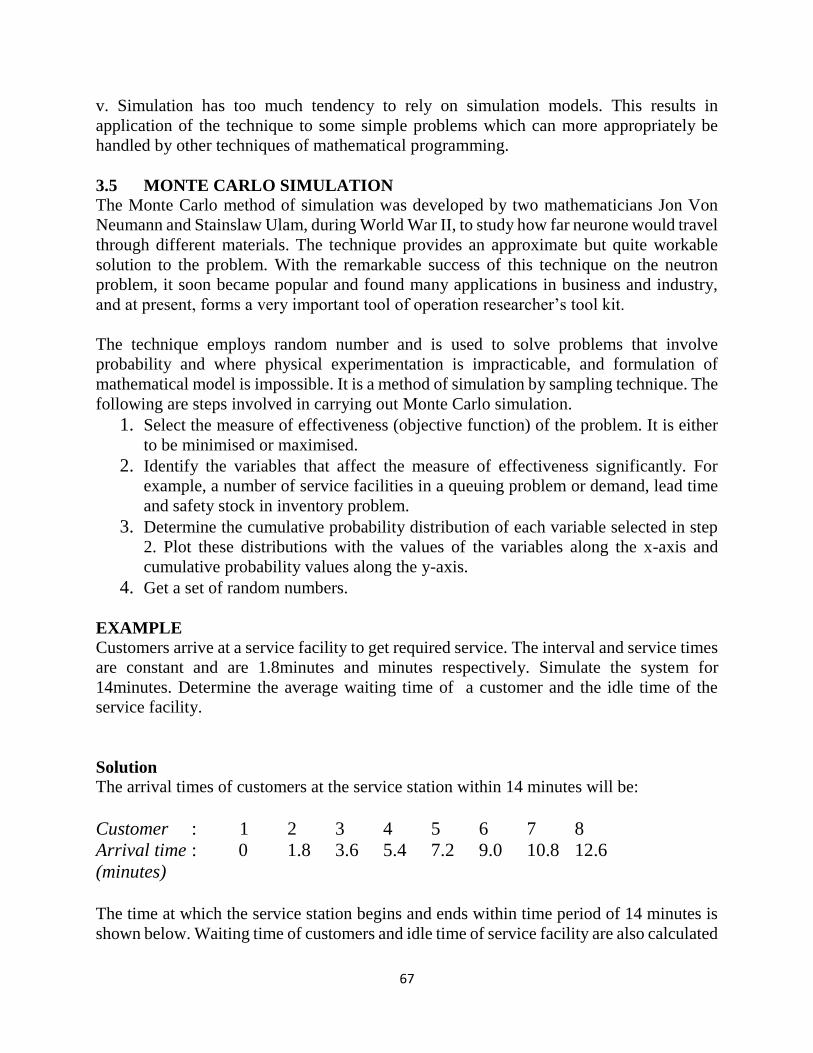
67

v. Simulation has too much tendency to rely on simulation models. This results in

application of the technique to some simple problems which can more appropriately be

handled by other techniques of mathematical programming.

3.5 MONTE CARLO SIMULATION

The Monte Carlo method of simulation was developed by two mathematicians Jon Von

Neumann and Stainslaw Ulam, during World War II, to study how far neurone would travel

through different materials. The technique provides an approximate but quite workable

solution to the problem. With the remarkable success of this technique on the neutron

problem, it soon became popular and found many applications in business and industry,

and at present, forms a very important tool of operation researcher’s tool kit.

The technique employs random number and is used to solve problems that involve

probability and where physical experimentation is impracticable, and formulation of

mathematical model is impossible. It is a method of simulation by sampling technique. The

following are steps involved in carrying out Monte Carlo simulation.

1. Select the measure of effectiveness (objective function) of the problem. It is either

to be minimised or maximised.

2. Identify the variables that affect the measure of effectiveness significantly. For

example, a number of service facilities in a queuing problem or demand, lead time

and safety stock in inventory problem.

3. Determine the cumulative probability distribution of each variable selected in step

2. Plot these distributions with the values of the variables along the x-axis and

cumulative probability values along the y-axis.

4. Get a set of random numbers.

EXAMPLE

Customers arrive at a service facility to get required service. The interval and service times

are constant and are 1.8minutes and minutes respectively. Simulate the system for

14minutes. Determine the average waiting time of a customer and the idle time of the

service facility.

Solution

The arrival times of customers at the service station within 14 minutes will be:

Customer : 1 2 3 4 5 6 7 8

Arrival time : 0 1.8 3.6 5.4 7.2 9.0 10.8 12.6

(minutes)

The time at which the service station begins and ends within time period of 14 minutes is

shown below. Waiting time of customers and idle time of service facility are also calculated

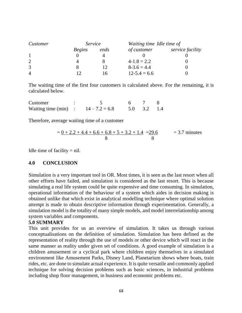
68

Customer Service Waiting time Idle time of

Begins ends of customer service facility

1 0 4 0 0

2 4 8 4-1.8 = 2.2 0

3 8 12 8-3.6 = 4.4 0

4 12 16 12-5.4 = 6.6 0

The waiting time of the first four customers is calculated above. For the remaining, it is

calculated below.

Customer : 5 6 7 8

Waiting time (min) : 14 – 7.2 = 6.8 5.0 3.2 1.4

Therefore, average waiting time of a customer

= 0 + 2.2 + 4.4 + 6.6 + 6.8 + 5 + 3.2 + 1.4 =29.6 = 3.7 minutes

8 8

Idle time of facility = nil.

4.0 CONCLUSION

Simulation is a very important tool in OR. Most times, it is seen as the last resort when all

other efforts have failed, and simulation is considered as the last resort. This is because

simulating a real life system could be quite expensive and time consuming. In simulation,

operational information of the behaviour of a system which aides in decision making is

obtained unlike that which exist in analytical modelling technique where optimal solution

attempt is made to obtain descriptive information through experimentation. Generally, a

simulation model is the totality of many simple models, and model interrelationship among

system variables and components.

5.0 SUMMARY

This unit provides for us an overview of simulation. It takes us through various

conceptualisations on the definition of simulation. Simulation has been defined as the

representation of reality through the use of models or other device which will react in the

same manner as reality under given set of conditions. A good example of simulation is a

children amusement or a cyclical park where children enjoy themselves in a simulated

environment like Amusement Parks, Disney Land, Planetarium shows where boats, train

rides, etc. are done to simulate actual experience. It is quite versatile and commonly applied

technique for solving decision problems such as basic sciences, in industrial problems

including shop floor management, in business and economic problems etc.

69


1. What do you understand by the term Simulation?

2. Explain six (6) advantages if Simulation.

3. Identify and explain five (5) areas of application of Simulation.

4. Give five limitations of Simulation.

7.0 REFERENCES



Company.

Jawahar, S. (2006). Overview of System Analysis & Design- Lesson Note no. 1, Ashok

Educational Foundation

Eiselt, H.A., and Sandblom, C. ( 2012). Operations Research: A Model Based

Approach, 2nd ed.,New York: Springer Heidelberg


Nigeria.

UNIT 8: CASES FOR OPERATIONS RESEARCH ANALYSIS

1.0 Introduction

2.0 Objectives

3.0 Main Content

3.1 Development of Operations Research

3.2 Definition of Operations Research

3.3 Characteristics of OR

3.4 Scientific Method In Operations Research

3.4.1 The Judgement Phase

3.4.2 The Research Phase

3.4.3 The Action Phase

70

3.5 Necessity of Operations Research in Industry

3.6 Scope of Operations Research

3.7 Scope of Operations Research in Financial Management

4.0 Conclusion

5.0 Summary


7.0 References

1.0 INTRODUCTION

We mentioned in Unit 1, module 1, that the subject Business Decision Analysis takes its

root from the discipline Operations Research or Operational Research (OR). This unit is

devoted to giving us background knowledge of OR. It is however, not going to be by any

way exhaustive as substantial literature been developed about quantitative approaches to

decision making. The root of this literature are centuries old, but much of it emerged only

during the past half century in tandem with the digital computer (Denardo, 2002). The

above assertion relates only to the development of the digital computer for use in solving

OR problems.

2.0 OBJECTIVES At the end of this study unit, you should be able to:

1 Briefly trace the development of OR.

2 Define OR.

3 Outline the characteristics of OR.

4 Give reasons why operations research is necessary in industries.

3.0 MAIN CONTENT

3.1 DEVELOPMENT OF OPERATIONS RESEARCH

Gupta and Hira (2012) traced the development of Operations Research (OR) thus:

i THE PERIOD BEFORE WORLD WAR II

The roots of OR are as old as science and society. Though the roots of OR extend to even

early 1800s, it was in 1885 when Ferderick, W. Taylor emphasized the application of

scientific analysis to methods of production, that the real start took place. Taylor conducted

experiments in connection with a simple shovel. His aim was to find that weight load of

Ore moved by shovel would result in the maximum amount of ore move with minimum

fatigue. After many experiments with varying weights, he obtained the optimum weight

load, which though much lighter than that commonly used, provided maximum movement

of ore during a day. For a “first-class man” the proper load turned out to be 20 pounds.

Since the density of Ore differs greatly, a shovel was designed for each density of Ore so

as to assume the proper weight when the shovel was correctly filled. Productivity rose

substantially after this change.

71

Henry L. Gantt, also of the scientific management era, developed job sequencing and

scheduling methods by mapping out each job from machine to machine, in order to

minimize delay. Now, with the Gantt procedure, it is possible to plan machine loading

months in advance and still quote delivery dates accurately.

However, the first industrial Revolution was the main contributing factor towards the

development of OR. Before this period, most of the industries were small scale, employing

only a handful of men. The advent of machine tools – the replacement of man by machine

as a source of power and improved means of transportation and communication resulted in

fast flourishing industries. If became increasingly difficult for a single man to perform all

the managerial functions (Planning, sales, purchasing production, etc). Consequently, a

division of management functions took place. Managers of production marketing, finance,

personal, research and development etc. began to appear. For example, production

department was sub-divided into sections like maintenance, quality control, procurement,

production planning etc.

ii WORLD WAR II During War II, the military management in England called on a team of scientists to study

the strategic and tactical problems of air and land defence. This team was under the

leadership of Professor P. M. S. Blackett of University of Manchester and a former Naval

Officer. “Blackett’s circus”, as the group was called, included three Physiologists, two

Mathematical Physicists, one Astrophysicist, one Army officer, one Surveyor, one general

physicist and two Mathematicians. The objective of this team was to find out the most

effective allocation of limited military resources to the various military operations and to

activities within each operation. The application included effective use of newly invented

radar, allocation of British Air Force Planes to missions and the determination best patters

for searching submarines. This group of scientist formed the first OR team..

iii POST WORLD WAR II

Immediately after the war, the success of military teams attracted the attention of industrial

mangers who were seeking solutions to their problems. Industrial operations research in

U.K and USA developed along different lines, and in UK the critical economic efficiency

and creation of new markets. Nationalisation of new key industries further increased the

potential field for OR. Consequently OR soon spread from military to government,

industrial, social and economic planning.

In the USA, the situation was different impressed by is dramatic success in UK, defence

operations research in USA was increased. Most of the war-experienced OR workers

remained in the military services. Industrial executives did not call for much help because

they were returning to peace and many of them believed that it was merely a new

72

applicati0on of an old technique. Operations research has been known by a variety of

names in that country such as Operational Analysis, Operations Evaluation, Systems

Analysis, Systems Evaluation, Systems Research, Decision Analysis, Quantitative

Analysis, Decision Science, and Management Science.

3.2 DEFINITION OF OPERATIONS RESEARCH Many definitions of OR have been suggested by writers and experts in the field of

operations Research. We shall consider a few of them.

1. Operations Research is the applications of scientific methods by inter disciplinary teams

to problems involving the control of organized (Man-Machine) Systems so as to provide

solutions which best serve the purpose of the organization as a whole (Ackoff & Sasieni,

1991).

2. Operations Research is applied decision theory. It uses any scientific, Mathematical or

Logical means to attempt to cope with the problems that confront the executive when he

tries to achieve a thorough going rationality in dealing with his decision problems (Miller

and Starr, 1973).

3. Operations research is a scientific approach to problem solving for executive

management (Wagner, 1973).

4. Operations Research is the art of giving bad answers to problems, to which, otherwise,

worse answers are given (Saaty, 1959).

3.3 CHARACTERISTICS OF OR

Ihemeje (2002) presents four vital characteristics of OR.

1. The OR approach is to develop a scientific model of the system under investigation with

which to compare the probable outcomes of alternative management decision or strategies.

2. OR is essentially an aid to decision making. The result of an operation study should have

a direct effect on managerial action, management decision based on the finding of an OR

model are likely to be more scientific and better informed.

3. It is based on the scientific method. It involves the use of carefully constructed models

based on some measurable variables. It is, in essence, a quantitative and logical approach

rather than a qualitative one. The dominant techniques of OR are mathematical and

statistical.

Other characteristics of OR are:

4. It is system (Executive) Oriented

5. It makes use of interdisciplinary teams

6. Application of scientific method

7. Uncovering of new problems

73

8. Improvement in quality of decision

3.4 SCIENTIFIC METHOD IN OPERATIONS RESEARCH Of these three phases, the research phase is the longest. The other two phases are equally

important as they provide the basis of the research phase. We now consider each phase

briefly as presented by Gupta & Hira (2012).

3.4.1 THE JUDGEMENT PHASE The judgement phases of the scientific method of OR consists of the following:

A. Determination of the Operation: An operation is the combination of different actions

dealing with resources (e.g men and machines) which form a structure from which an

action with regards to broader objectives is maintained. For example an act of assembling

an engine is an operation.

B. Determination of Objectives and Values Associated with the operation: In the

judgement phase, due care must be given to define correctly the frame of references of

operations. Efforts should be made to find the type of situation, e.g manufacturing,

engineering, tactical, strategic etc.

C. Determination of Effectiveness Measures: The measure of effectiveness implies the

measure of success of a model in representing a problem and providing a solution. It is the

connecting link between the objectives and the analysis required for corrective action.

3.4.2 THE RESEARCH PHASE

The research phase of OR includes the following:

a. Observation and Data Collection: This enhances better understanding of the problem.

b. Formulation of Relevant Hypothesis: Tentative explanations, when formulated as

propositions are called hypothesis. The formulation of a good hypothesis depends upon

the sound knowledge of the subject–matter. A hypothesis must provide an answer to the

problem in question.

c. Analysis of Available Information and Verification of Hypothesis: Quantitative as well

as qualitative methods may be used to analyse available data.

d. Prediction and Generalisation of Results and Consideration of Alternative Methods:

Once a model has been verified, a theory is developed from the model to obtain a complete

description of the problem. This is done by studying the effect of changes in the parameters

of the model. The theory so developed may be used to extrapolate into the future.

3.4.3 THE ACTION PHASE

The action phase consists of making recommendations for remedial action to those who

first posed the problem and who control the operations directly. These recommendations

74

consists of a clear statement of the assumptions made, scope and limitations of the

information presented about the situation, alternative courses of action, effects of each

alternative as well as the preferred course of action.

A primary function of OR group is to provide an administrator with better understanding

of the implications of the decisions he makes. The scientific method supplements his ideas

and experiences and helps him to attain his goals fully.

3.5 NECESSITY OF OPERATIONS RESEARCH IN INDUSTRY Having studied the scientific methods of operations research, we now focus on why OR is

important or necessary in industries. OR came into existence in connection with war

operations, to decide the strategy by which enemies could be harmed to the maximum

possible extent with the help of the available equipment. War situations required reliable

decision making. But the need for reliable decision techniques is also needed by industries

for the following reasons.

Complexity: Today, industrial undertakings have become large and complex. This

is because the scope of operations has increased. Many factors interact with each

other in a complex way. There is therefore a great uncertainty about the outcome of

interaction of factors like technological, environmental, competitive etc. For

instance, a factory production schedule will take the following factors into account:

i. Customer demand.

ii. Raw material requirement.

iii. Equipment Capacity and possibility of equipment failure.

iv. Restrictions on manufacturing processes.

It could be seen that, it is not easy to prepare a schedule which is both economical and

realistic. This needs mathematical models, which in addition to optimization, help to

analyse the complex situation. With such models, complex problems can be split into

simpler parts, each part can be analysed separately and then the results can be synthesized

to give insights into the problem.

Scattered Responsibility and Authority: In a big industry, responsibility and

authority of decision-making is scattered throughout the organization and thus the

organization, if it is not conscious, may be following inconsistent goals.

Mathematical quantification of OR overcomes this difficulty to a great extent.

Uncertainty: There is a lot of uncertainty about economic growth. This makes each

decision costlier and time consuming. OR is essential from the point of view of

reliability.

3.6 SCOPE OF OPERATIONS RESEARCH

75

We now turn our attention towards learning about the areas that OR covers. OR as a

discipline is very broad and is relevant in the following areas.

In Industry: OR is relevant in the field or industrial management where there is a

chain of problems or decisions starting from the purchase of raw materials to the

dispatch of finished goods. The management is interested in having an overall view

of the method of optimizing profits. In order to take scientific decisions, an OR team

will have to consider various alternative methods of producing the goods and the

returns in each case. OR should point out the possible changes in overall structure

like installation of a new machine, introduction of more automation etc.

Also, OR has been successfully applied in production, blending, product mix,

inventory control, demand forecast, sales and purchases, transportation, repair and

maintenance, scheduling and sequencing, planning, product control, etc.

In Defence: OR has wide application in defence operations. In modern warfare, the

defence operations are carried out by a number of different agencies, namely – Air

force, Army, and Navy. The activities perfumed by each of these agencies can

further be divided into sub-activities viz: operations, intelligence, administration,

training, etc. There is thus a need to coordinate the various activities involved in

order to arrive at an optimum strategy and to achieve consistent goals.

In Management: Operations Research is a problem-solving and decision-

making science. It is a tool kit for scientific and programmable rules providing the

management a qualitative basis for decision making regarding the operations under

its control. Some of the area of management where OR techniques have been

successfully applied are as follows:

A. Allocation and Distribution

i. Optimal allocation of limited resources such as men, machines, materials, time, and

money.

ii. Location and size of warehouses, distribution centres retail depots etc

iii. Distribution policy

B. Production and Facility Planning

i. Selection, location and design of production plants, distribution centre and retail outlets.

ii. Project scheduling and allocation of resources.

iii. Preparation of forecast for the various inventory items and computing economic order

quantities and reorder levels.

iv. Determination of number and size of the items to be produced.

C. Procurement

i. What, how, and when to purchase at minimum purchase cost.

76

ii. Bidding and replacement policies.

iii. Transportation planning and vendor analysis.

D. Marketing

i. Product selection, timing, and competitive actions.

ii. Selection of advertisement media.

iii. Demand forecast and stock levels.

E. Finance

i. Capital requirement, cash-flow analysis.

ii. Credit policy, credit risks etc.

iii. Profit plan for the organisation.

F. Personnel

i. Selection of personnel, determination of retirement age and skills.

ii. Recruitment policies and assignment of jobs.

iii. Wages/salaries administration.

G. Research and Development

i. Determination of areas for research and development.

ii. Reliability and control of development projects.

iii. Selection of projects and preparation of budgets.

3.7 SCOPE OF OPERATIONS RESEARCH IN FINANCIAL MANAGEMENT

The scope of OR in financial management covers the following areas

i. Cash Management: Linear programming techniques are helpful in determining the

allocation of funds to each section.

ii. Inventory Control: Inventory control techniques of OR can help management to

develop better inventory policies and bring down the investment in inventories. These

techniques help to achieve optimum balance between inventory carrying costs and shortage

cost.

iii. Simulation Technique: Simulation considers various factors that affect and present

and projected cost of borrowing money from commercial banks, and tax rates etc. and

provides an optimum combination of finance (debt, equity, retained earnings) for the

desired amount of capital.

iv. Capital Budgeting

It involves evaluation of various investment proposals (viz, market introduction of new

products and replacement of equipment with a new one).

4.0 CONCLUSION

Operations Research as we know it today, as developed during War II, when the military

management in England called on a team of scientists to study the strategic and tactical

problems of air and land defence. Ever since that period, the impact of Operations Research

77

can be felt in many areas. This is shown by the ever increasing member of educational

institutions offering it at degree level.

5.0 SUMMARY

This has provided us with background information on the area of Operations Research. As

stated in the opening unit of this study material, the discipline Business Decision Analysis

or Analysis for Business Decisions takes its root from operations research. The History and

Development of operations research which is as old as science and society. Though the

roots of or extend to even early 1800s, it was in 1885 when Ferderick, w. Taylor

emphasized the application of scientific analysis to methods of production, that the real

start took place. Taylor conducted experiments in connection with a simple shovel.

However, Operations Research as we know it today can be traced to the period during War

II, when the military management in England called on a team of scientists to study the

strategic and tactical problems of air and land defence.


Trace the history and development of operations to the founding fathers of the field

of management.

Give two definitions of operations research with identified authors.

Identify the four main characteristics of operations research.

Identify and briefly discuss the phases involved in the Scientific Method in

Operations research.

7.0 REFERENCES

Ackoff, R., and Sisieni, M. (1991). Fundamentals of Operations Research, New York: John

Wiley and Sons Inc.

Churchman, C.W., Ackoff, R.L., and Arnoff, E.L.(1957). Introduction to Operations

Research, New York: John Wiley and Sons Inc.




Company.

Ihemeje, J.C. (2002). Fundamentals of Business Decision Analysis, Lagos- Sibon Books


Nigeria.

78

MODULE THREE

UNIT 9: MATHEMATICAL PROGRAMMING (LINEAR PROGRAMMING)

1.0 Introduction

2.0 Objectives

3.0 Main Content

3.1 Requirements for Linear Programming Problems

3.2 Assumptions in Linear Programming

3.3 Application of Linear Programming

3.4 Areas of Application of Linear Programming

3.5 Formulation of Linear Programming Problems

3.6 Advantages Linear Programming Methods

3.7 Limitation of Linear programming Models

3.8 Graphical Methods of Linear Programming Solution

4.0 Conclusion

5.0 Summary


79

7.0 References

1.0 INTRODUCTION

Linear programming deals with the optimization (maximization or minimization) of a

function of variables known as objective function, subject to a set of linear equations and/or

inequalities known as constraints. The objective function may be profit, cost, production

capacity or any other measure of effectiveness, which is to be obtained in the best possible

or optimal manner. The constraints may be imposed by different resources such as market

demand, production process and equipment, storage capacity, raw material availability, etc.

By linearity is meant a mathematical expression in which the expressions among the

variables are linear e.g., the expression a1x1 + a2x2 + a3x3 + ... + aⁿxⁿ is linear. Higher powers

of the variables or their products do not appear in the expressions for the objective function

as well as the constraints (they donot have expressions like x13, x2

3/2, x1x2, a1x1 + a2 log x2,

etc.). The variables obey the properties of proportionality (e.g., if a product requires 3 hours

of machining time, 5 units of it will require 15 hours) and additivity (e.g., amount of a

resource required for a certain number of products is equal to the sum of the resource

required for each).

It was in 1947 that George Dantzig and his associates found out a technique for solving

military planning problems while they were working on a project for U.S. Air Force. This

technique consisted of representing the various activities of an organization as a linear

programming (L.P.) model and arriving at the optimal programme by minimizing a linear

objective function. Afterwards, Dantzig suggested this approach for solving business and

industrial problems. He also developed the most powerful mathematical tool known as

“simplex method” to solve linear programming problems.

2.0 OBJECTIVES

At the end of this study unit, you should be able to

1. Explain the requirements for Linear Programming

2. Highlight the assumptions of Linear Programming

3. Identify the Areas of application of Linear Programming

4. Formulate a Linear Programming problem

5. Solve various problems using Linear Programming

3.0 MAIN CONTENT

3.1 REQUIREMENTS FOR A LINEAR PROGRAMMING PROBLEM

All organizations, big or small, have at their disposal, men, machines, money and materials,

the supply of which may be limited. If the supply of these resources were unlimited, the

need for management tools like linear programming would not arise at all. Supply of

resources being limited, the management must find the best allocation of its resources in

80

order to maximize the profit or minimize the loss or utilize the production capacity to the

maximum extent. However this involves a number of problems which can be overcome by

quantitative methods, particularly the linear programming.

Generally speaking, linear programming can be used for optimization problems if the

following conditions are satisfied:

1. There must be a well-defined objective function (profit, cost or quantities produced)

which is to be either maximized or minimized and which can be expressed as a linear

function of decision variables.

2. There must be constraints on the amount or extent of attainment of the objective and

these constraints must be capable of being expressed as linear equations or inequalities in

terms of variables.

3. There must be alternative courses of action. For example, a given product may be

processed by two different machines and problem may be as to how much of the product

to allocate to which machine.

4. Another necessary requirement is that decision variables should be interrelated and

nonnegative. The non-negativity condition shows that linear programming deals with real

life situations for which negative quantities are generally illogical.

3.2 ASSUMPTIONS IN LINEAR PROGRAMMING MODELS

A linear programming model is based on the following assumptions:

1. Proportionality: A basic assumption of linear programming is that proportionality exists

in the objective function and the constraints. This assumption implies that if a product

yields a profit of #10, the profit earned from the sale of 12 such products will be # (10 x

12) = #120. This may not always be true because of quantity discounts. Further, even if the

sale price is constant, the manufacturing cost may vary with the number of units produced

and so may vary the profit per unit. Likewise, it is assumed that if one product requires

processing time of 5 hours, then ten such products will require processing time of 5 x 10 =

50 hours. This may also not be true as the processing time per unit often decreases with

increase in number of units produced. The real world situations may not be strictly linear.

However, assumed linearity represents their close approximations and provides very useful

answers.

2. Additivity: It means that if we use t1 hours on machine A to make product 1 and t2 hours

to make product 2, the total time required to make products 1 and 2 on machine A is t1 + t2

hours. This, however, is true only if the change-over time from product 1 to product 2 is

negligible. Some processes may not behave in this way. For example, when several liquids

of different chemical compositions are mixed, the resulting volume may not be equal to

the sum of the volumes of the individual liquids.

81

3. Continuity: Another assumption underlying the linear programming model is that the

decision variables are continuous i.e., they are permitted to take any non-negative values

that satisfy the constraints. However, there are problems wherein variables are restricted to

have integral values only. Though such problems, strictly speaking, are not linear

programming problems, they are frequently solved by linear programming techniques and

the values are then rounded off to nearest integers to satisfy the constraints. This

approximation, however, is valid only if the variables have large optimal values. Further,

it must be ascertained whether the solution represented by the rounded values is a feasible

solution and also whether the solution is the best integer solution.

4. Certainty: Another assumption underlying a linear programming model is that the

various parameters, namely, the objective function coefficients, R.H.S. coefficients of the

constraints and resource values in the constraints are certainly and precisely known and

that their values do not change with time. Thus the profit or cost per unit of the product,

labour and materials required per unit, availability of labour and materials, market demand

of the product produced, etc. are assumed to be known with- certainty. The linear

programming problem is, therefore, assumed to be deterministic in nature.

5. Finite Choices: A linear programming model also assumes that a finite (limited) number

of choices (alternatives) are available to the decision-maker and that the decision variables

are interrelated and non-negative. The non-negativity condition shows that linear

programming deals with real-life situations as it is not possible to produce/use negative

quantities.

Mathematically these non-negativity conditions do not differ from other constraints.

However, since while solving the problems they are handled differently from the other

constraints, they are termed as non-negativity restrictions and the term constraints is used

to represent constraints other than non-negativity restrictions and this terminology has been

followed throughout the book.

3.3 APPLICATIONS OF LINEAR PROGRAMMING METHOD

Though, in the world we live, most of the events are non-linear, yet there are many

instances of linear events that occur in day-to-day life. Therefore, an understanding of

linear programming and its application in solving problems is utmost essential for today’s

managers.

Linear programming techniques are widely used to solve a number of business, industrial,

military, economic, marketing, distribution and advertising problems. Three primary

reasons for its wide use are:

1. A large number of problems from different fields can be represented or at least

approximated to linear programming problems.

2. Powerful and efficient techniques for solving L.P. problems are available.

82

3. L.P. models can handle data variation (sensitivity analysis) easily.

However, solution procedures are generally iterative and even medium size problems

require manipulation of large amount of data. But with the development of digital

computers, this disadvantage has been completely overcome as these computers can handle

even large L.P. problems in comparatively very little time at a low cost.

3.4 AREAS OF APPLICATION OF LINEAR PROGRAMMING

Linear programming is one of the most widely applied techniques of operations research

in business, industry and numerous other fields. A few areas of its application are given

below.

1. INDUSTRIAL APPLICATIONS

(a) Product mix problems: An industrial concern has available a certain production

capacity (men, machines, money, materials, market, etc.) on various manufacturing

processes to manufacture various products. Typically, different products will have different

selling prices, will require different amounts of production capacity at the several processes

and will, therefore, have different unit profits; there may also be stipulations (conditions)

on maximum and/or minimum product levels. The problem is to determine the product mix

that will maximize the total profit.

(b) Blending problems: These problems are likely to arise when a product can be made

from a variety of available raw materials of various compositions and prices. The

manufacturing process involves blending (mixing) some of these materials in varying

quantities to make a product of the desired specifications.

(c) Production scheduling problems: They involve the determination of optimum

production schedule to meet fluctuating demand. The objective is to meet demand, keep

inventory and employment at reasonable minimum levels, while minimizing the total cost

Production and inventory.

(d) Trim loss problems: They are applicable to paper, sheet metal and glass manufacturing

industries where items of standard sizes have to be cut to smaller sizes as per customer

requirements with the objective of minimizing the waste produced.

(e) Assembly-line balancing: It relates to a category of problems wherein the final product

has a number of different components assembled together. These components are to be

assembled in a specific sequence or set of sequences. Each assembly operator is to be

assigned the task / combination of tasks so that his task time is less than or equal to the

cycle time.

2. MANAGEMENT APPLICATIONS

83

(a) Media selection problems: They involve the selection of advertising mix among

different advertising media such as T.V., radio, magazines and newspapers that will

maximize public exposure to company’s product. The constraints may be on the total

advertising budget, maximum expenditure in each media, maximum number of insertions

in each media and the like.

(b) Portfolio selection problems: They are frequently encountered by banks, financial

companies, insurance companies, investment services, etc. A given amount is to be

allocated among several investment alternatives such as bonds, saving certificates,

common stock, mutual fund, real estate, etc. to maximize the expected return or minimize

the expected risk.

(c) Profit planning problems: They involve planning profits on fiscal year basis to

maximize profit margin from investment in plant facilities, machinery, inventory and cash

on hand.

(d) Transportation problems: They involve transportation of products from, say, n

sources situated at different locations to, say, m different destinations. Supply position at

the sources, demand at destinations, freight charges and storage costs, etc. are known and

the problem is to design the optimum transportation plan that minimizes the total

transportation cost (or distance or time).

(e) Assignment problems: They are concerned with allocation of facilities (men or

machines) to jobs. Time required by each facility to perform each job is given and the

problem is to find the optimum allocation (one job to one facility) so that the total time to

perform the jobs is minimized.

3.5 FORMULATION OF LINEAR PROGRAMMING PROBLEMS

First, the given problem must be presented in linear programming form. This requires

defining the variables of the problem, establishing inter-relationships between them and

formulating the objective function and constraints. A model, which approximates as closely

as possible to the given problem, is then to be developed. If some constraints happen to be

nonlinear, they are approximated to appropriate linear functions to fit the linear

programming format. In case it is not possible, other techniques may be used to formulate

and then solve the model.

EXAMPLE 1 (Production Allocation Problem)

A firm produces three products. These products are processed on three different machines.

The time required to manufacture one unit of each of the three products and the daily

capacity of the three machines are given in the table below.

TABLE 1

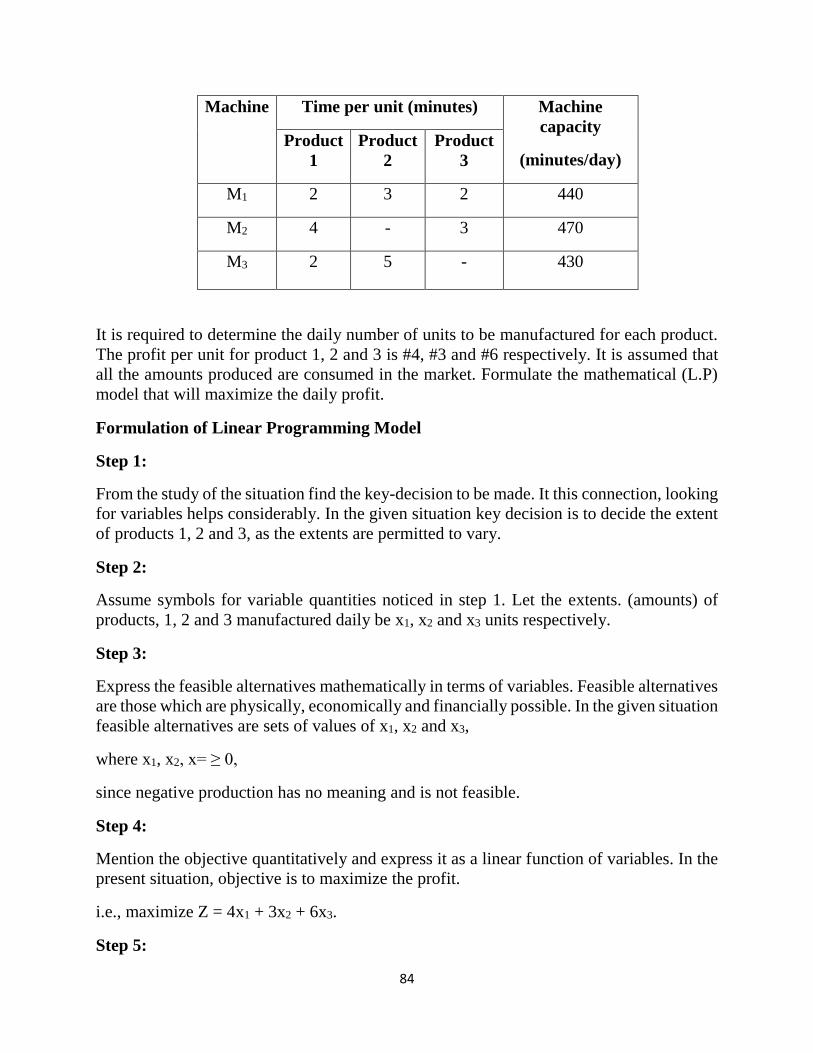
84

Machine Time per unit (minutes) Machine

capacity

(minutes/day)

Product

1

Product

2

Product

3

M1 2 3 2 440

M2 4 - 3 470

M3 2 5 - 430

It is required to determine the daily number of units to be manufactured for each product.

The profit per unit for product 1, 2 and 3 is #4, #3 and #6 respectively. It is assumed that

all the amounts produced are consumed in the market. Formulate the mathematical (L.P)

model that will maximize the daily profit.

Formulation of Linear Programming Model

Step 1:

From the study of the situation find the key-decision to be made. It this connection, looking

for variables helps considerably. In the given situation key decision is to decide the extent

of products 1, 2 and 3, as the extents are permitted to vary.

Step 2:

Assume symbols for variable quantities noticed in step 1. Let the extents. (amounts) of

products, 1, 2 and 3 manufactured daily be x1, x2 and x3 units respectively.

Step 3:

Express the feasible alternatives mathematically in terms of variables. Feasible alternatives

are those which are physically, economically and financially possible. In the given situation

feasible alternatives are sets of values of x1, x2 and x3,

where x1, x2, x= ≥ 0,

since negative production has no meaning and is not feasible.

Step 4:

Mention the objective quantitatively and express it as a linear function of variables. In the

present situation, objective is to maximize the profit.

i.e., maximize Z = 4x1 + 3x2 + 6x3.

Step 5:

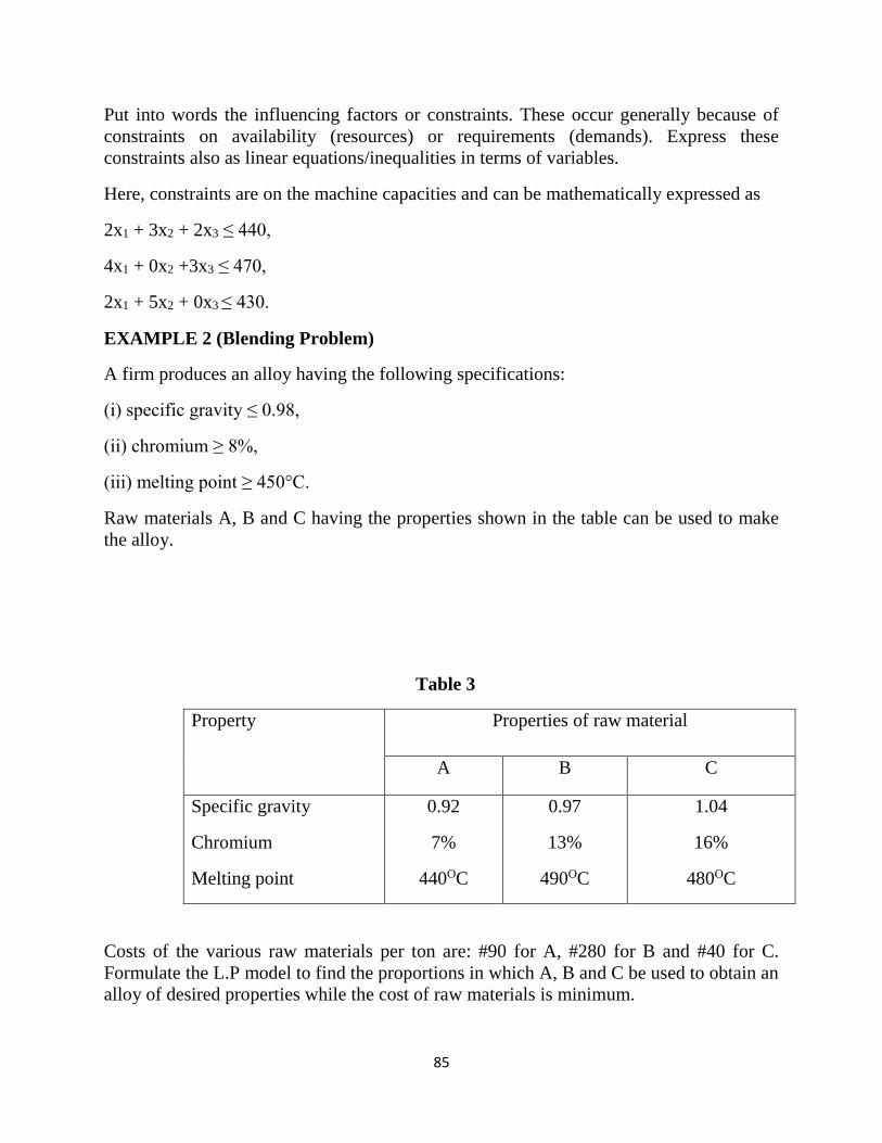
85

Put into words the influencing factors or constraints. These occur generally because of

constraints on availability (resources) or requirements (demands). Express these

constraints also as linear equations/inequalities in terms of variables.

Here, constraints are on the machine capacities and can be mathematically expressed as

2x1 + 3x2 + 2x3 ≤ 440,

4x1 + 0x2 +3x3 ≤ 470,

2x1 + 5x2 + 0x3 ≤ 430.

EXAMPLE 2 (Blending Problem)

A firm produces an alloy having the following specifications:

(i) specific gravity ≤ 0.98,

(ii) chromium ≥ 8%,

(iii) melting point ≥ 450°C.

Raw materials A, B and C having the properties shown in the table can be used to make

the alloy.

Table 3

Property Properties of raw material

A B C

Specific gravity

Chromium

Melting point

0.92

7%

440OC

0.97

13%

490OC

1.04

16%

480OC

Costs of the various raw materials per ton are: #90 for A, #280 for B and #40 for C.

Formulate the L.P model to find the proportions in which A, B and C be used to obtain an

alloy of desired properties while the cost of raw materials is minimum.

86


Let the percentage contents of raw materials A, B and C to be used for making the alloy be

x1, x2 and x3 respectively.

Objective is to minimize the cost

i.e., minimize Z = 90x1 + 280x2 + 40x3.

Constraints are imposed by the specifications required for the alloy.

They are

0.92x1 + 0.97x2 + 1.04x3 ≤ 0.98,

7x1 + 13x2+ 16x3 ≥ 8,

440x1 + 490x2 + 480x3 ≥ 450,

and x1 + x2 + x3 = 100,

as x1, x2 and x3 are the percentage contents of materials A, B and C in making the alloy.

Also x1, x2, x3, each ≥ 0.


Let x1, x2, x3 and x4 denote the number of advertising units to be bought on television,

radio, magazine I and magazine II respectively.

The objective is to maximize the total number of potential customers reached.

i.e., maximize Z = 10 (2x1 + 6x2 + 1.5x3 + x4).

Constraints are on the advertising budget: 30,000x1+20,000x2+15,000x3+10,000x4 ≤

450,000

or 30x1+20x2+15x3+10x4 ≤ 450,

on number of female customers reached by the advertising campaign:

150,000x1+400,000x2+70,000x3+50,000x4= ≥ 100,000

or 15x1+40x2+7x3+5x4 ≥ 100

on expenses on magazine advertising: 15,000x3+10,000x4 ≤ 150,000 or 15x3+10x4 ≤

150

on no. of units on magazines: x3 ≥ 3,

87

x4 ≥ 2,

on no. of units on television: : 5 ≤ x1 ≤ 10 or x1 ≥ 5, x1 ≤ 10

on no. of units on radio: 5 ≤ x2 ≤ 10 or x2 ≥ 5, x2 ≤ 10

where x1, x2, x3, x4, each ≥ 0.

EXAMPLE 3 (Inspection Problem)

A company has two grades of inspectors, I and II to undertake quality control inspection.

At least 1,500 pieces must be inspected in an 8-hour day. Grade I inspector can check 20

pieces in an hour with an accuracy of 96%. Grade II inspector checks 14 pieces an hour

with an accuracy of 92%.

Wages of grade I inspector are #5 per hour while those of grade II inspector are #4 per

hour. Any error made by inspector costs #3 to the company. If there are, in all, 10 grade I

inspectors and 15 grade II inspectors in the company find the optimal assignment of

inspectors that minimizes the daily inspection cost.

Formulation of L.P Model

Let x1 and x2 denote the number of grade I and grade II inspectors that may be assigned the

job of quality control inspection.

The objective is to minimize the daily cost of inspection. Now the company has to incur

two types of costs: wages paid to the inspectors and the cost of their inspection errors. The

cost of grade I inspector/hour is;

# (5 + 3 x 0.04 x 20) = #7.40.

Similarly, cost of grade II inspector/hour is

# (4 + 3 x 0.08 x 14) = #7.36.

: The objective function is

minimize Z = 8(7.40x1 + 7.36x2) = 59.20x1 + 58.88x2.

Constraints are on the number of grade I inspectors: x1 ≤ 10,

on the number of grade II inspectors : x2 ≤ 15,

on the number of pieces to be inspected daily:

20 X 8x1 + 14 X 8x2 ≥ 1,500

or 160x1 + 112x2 ≥ 1,500,

88

where x1,x2 ≥ 0.

EXAMPLE 4 (Product Mix Problem)

Consider the following problem faced by a production planner in a soft drink plant. He has

two bottling machines A and B. A is designed for 8-ounce bottles and B for 16-ounce

bottles. However; each can be used on both types of Bottles with some lass of efficiency.

The following data are available:

Machine 8-ounce bottles 16-ounce bottles

A 100/minute 40/minute

B 60/minute 75/minute

The machines can be run 8-hour per day, 5 days a week. Profit on 8-ounce bottle is 15 paise

and on 16-ounce bottle is 25 paise. Weekly production of the drink cannot exceed 300,000

ounces and the market can absorb 25,000 eight-ounce bottles and 7,000 sixteen-ounce

bottles per week. The planner wishes to maximize his profit subject, of course, to all the

production and marketing constraints. Formulate this as L.P problem.


Key decision is to determine the number of 8-ounce bottles and 16-ounce bottles to be

produced on either of machines A and B per week. Let xA1, xB1 be the number of 8-ounce

bottles and xA2, xB2 be the number of 16-ounce bottles to be produced per week on

machines A and B respectively.

Objective is to maximize .the weekly profit.

i.e., maximize Z = #[0.15 (xA1 +xB1) + 0.25(xA2 +xB2)].

Constraints can be formulated as follows:

Since an 8-ounce bottle takes 1/100minute and a 16-ounce bottle takes 1/40 minute on

machine A and the machine can be run for 8 hours a day and 5 days a week, the time

constraint on machine A can be written as

xA1+ xA2≤ 5 X 8 X 60

100 40

≤ 2,400

Similarly, time constraint on machine B can be written as

89

xB1+ xB2≤ 2,400.

60 75

Since the total weekly production cannot exceed 300,000 ounces,

8(xA1+XB1) + 16(xA2 + xB2) ≤ 300,000.

The constraints on market demand yield

xA1 + xB1 ≥ 25,000,

xA2 + xB2 ≥ 7,000,

where xA1, xB1, xA2, xB2, each ≥ 0.

3.6 ADVANTAGES OF LINEAR PROGRAMMING METHODS

Following are the main advantages of linear programming methods:

1. It helps in attaining the optimum use of productive factors. Linear programming

indicates how a manager can utilize his productive factors most effectively by a better

selection and distribution of these elements. For example, more efficient use of manpower

and machines can be obtained by the use of linear programming.

2. It improves the quality of decisions. The individual who makes use of linear

programming methods becomes more objective than subjective. The individual having a

clear picture of the relationships within the basic equations, inequalities or constraints can

have a better idea about the problem and its solution.

3. It also helps in providing better tools for adjustments to meet changing conditions. It can

go a long way in improving the knowledge and skill of future executives.

4. Most business problems involve constraints like raw materials availability, market

demand, etc. which must be taken into consideration. Just because we can produce so many

units of products does not mean that they can be sold. Linear programming can handle such

situations also since it allows modification of its mathematical solutions.

3.7 LIMITATIONS OF LINEAR PROGRAMMING MODEL

This model, though having a wide field, has the following limitations:

1. For large problems having many limitations and constraints, the computational

difficulties are enormous, even when assistance of large digital computers is available. The

approximations required to reduce such problems to meaningful sizes may yield the final

results far different from the exact ones.

2. Another limitation of linear programming is that it may yield fractional valued answers

for the decision variables, whereas it may happen that only integer values of the variables

are logical.

90

For instance, in finding how many lathes and milling machines to be produced, only integer

values of the decision variables, say x1 and x2 are meaningful. Except when the variables

have large values, rounding the solution values to the nearest integers will not yield an

optimal solution. Such situations justify the use of special techniques like integer

programming.

3. It is applicable to only static situations since it does not take into account the effect of

time. The O.R. team must define the objective function and constraints which can change

due to internal as well as external factors.

3.8 GRAPHICAL METHOD OF SOLUTION

Once a problem is formulated as mathematical model, the next step is to solve the problem

to get the optimal solution. A linear programming problem with only two variables presents

a simple case, for which the solution can be derived using a graphical or geometrical

method. Though, in actual practice such small problems are rarely encountered, the

graphical method provides a pictorial representation of the solution process and a great

deal of insight into the basic concepts used in solving large L.P. problems. This method

consists of the following steps:

1. Represent the given problem in mathematical form i.e., formulate the mathematical

model for the given problem.

2. Draw the x1 and x2-axes. The non-negativity restrictions x1 ≥ 0 and x2 ≥ 0 imply that the

values of the variables x1 and x2 can lie only in the first quadrant. This eliminates a number

of infeasible alternatives that lie in 2nd, 3rd and 4th quadrants.

3. Plot each of the constraint on the graph. The constraints, whether equations or

inequalities are plotted as equations. For each constraint, assign any arbitrary value to one

variable and get the value of the other variable. Similarly, assign another arbitrary value to

the other variable and find the value of the first variable. Plot these two points and connect

them by a straight line. Thus each constraint is plotted as line in the first quadrant.

4. 1dentify the feasible region (or solution space) that satisfies all the constraints

simultaneously. For type constraint, the area on or above the constraint line i.e., away from

the origin and for type constraint, the area on or below the constraint line i.e., towards

origin will be considered. The area common to all the constraints is called feasible region

and is shown shaded. Any point on or within the shaded region represents a feasible

solution to the given problem. Though a number of infeasible points are eliminated, the

feasible region still contains a large number of feasible points

4.0 CONCLUSION

Linear programming involves with the optimization (maximization or minimization) of a

function of variables known as objective function, subject to a set of linear equations and/or

91

inequalities known as constraints. The objective function may be profit, cost, production

capacity or any other measure of effectiveness, which is to be obtained in the best possible

or optimal manner. The constraints may be imposed by different resources such as market

demand, production process and equipment, storage capacity, raw material availability and

so on.

5.0 SUMMARY

All organizations, big or small, have at their disposal, men, machines, money and materials,

the supply of which may be limited. If the supply of these resources were unlimited, the

need for management tools like linear programming would not arise at all. Supply of

resources being limited, the management must find the best allocation of its resources in

order to maximize the profit or minimize the loss or utilize the production capacity to the

maximum extent. However this involves a number of problems which can be overcome by

quantitative methods, particularly the linear programming. Generally speaking, linear

programming can be used for optimization problems if the following conditions are

satisfied- there must be a well-defined objective function; there must be constraints on the

amount or extent of attainment of the objective and these constraints must be capable of

being expressed as linear equations or inequalities in terms of variables; there must be

alternative courses of action; decision variables should be interrelated and nonnegative;

and the resources must be in limited supply. Linear Programming has the following

assumptions- Proportionality, Additivity, Continuity, Certainty, and Finite Choices. LP

solution methods can be applied in solving industrial problems, management related

problems, and a host of other problem areas.


Briefly discuss what linear programming involves.

Identify and discuss five assumptions of linear programming.

List and explain three areas where linear programming can be applied.

7.0 REFERENCES

Dixon – Ogbechi, B.N (2001). Decision Theory in Business, Lagos: Philglad Nig. Ltd.

Denardo, Eric V. (2002). The Schience of Decision making: A Problem-Based Approach



Company.


Publications.

92


Nigeria.

UNIT 10: TRANSPORTATION MODEL 1.0 Introduction

2.0 Objectives

3.0 Main Content

3.1 Assumptions Made in the Use of the Transportation Model

3.2 Theoretical Consideration

3.3 General Procedure for Setting Up a Transportation Model

3.4 Developing an Initial Solution

3.4.1 The North West Corner Method

93

3.4.2 The Least Cost Method

3.4.3 Vogel’s Approximation Method (VAM)

3.5 The Unbalanced Case

3.6 Formulating Linear Programming Model for the Transportation Problem

3.7 Improving the Initial Feasible Solution Through Optimization

3.8 Determination of the Optimal Transportation Cost Using the Stepping

Stone Method

3.9 The Modified Distribution Method

3.10 Degeneracy

4.0 Conclusion

5.0 Summary


7.0 References

1.0 INTRODUCTION

The transportation problem is a special type of linear programming problem. It deals

withthe distribution of goods from the various points of supply, such as factories, often

knownas sources, to a number of points of demand, such as warehouses, often known

asdestinations. Each source is able to supply a fixed number of units of the product,

usuallycalled capacity or availability and each destination has a fixed demand, usually

called therequirements. The objective is to schedule shipments from sources to destinations

so thattransportation cost is a minimum. The transportation problem has been used in

variedtypes of practical applications such as product allocation, machine assignment and

product distribution, in an effort to minimize costs of distribution and!or allocation and

optimize distribution efficiency.

2.0 OBJECTIVES

After completing this chapter, you should be able to:

Describe the nature of a transportation problem.

Compute the initial feasible solution using the North West Corner method.

Find the initial feasible solution using the Least Cost Method.

Compute the initial feasible solution using the Vogel’s Approximation Method.

Use the Stepping Stones and Modified Distribution Methods to find the optimum

solution.

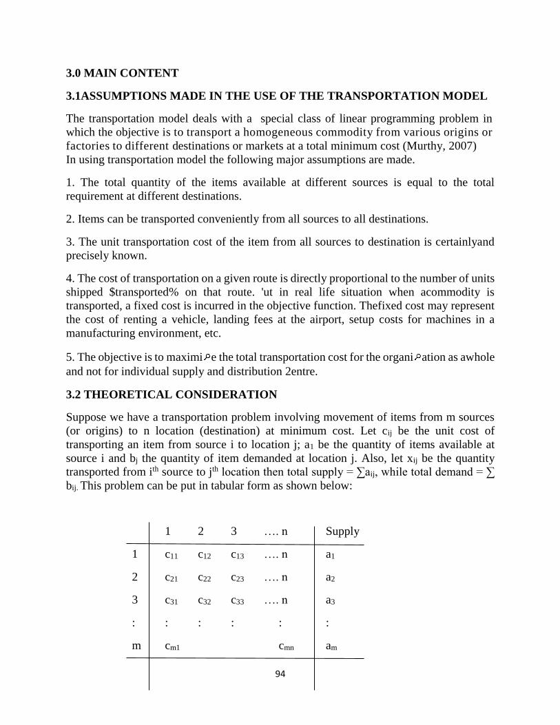
94

3.0 MAIN CONTENT

3.1ASSUMPTIONS MADE IN THE USE OF THE TRANSPORTATION MODEL

The transportation model deals with a special class of linear programming problem in

which the objective is to transport a homogeneous commodity from various origins or

factories to different destinations or markets at a total minimum cost (Murthy, 2007)

In using transportation model the following major assumptions are made.

1. The total quantity of the items available at different sources is equal to the total

requirement at different destinations.

2. Items can be transported conveniently from all sources to all destinations.

3. The unit transportation cost of the item from all sources to destination is certainlyand

precisely known.

4. The cost of transportation on a given route is directly proportional to the number of units

shipped $transported% on that route. 'ut in real life situation when acommodity is

transported, a fixed cost is incurred in the objective function. Thefixed cost may represent

the cost of renting a vehicle, landing fees at the airport, setup costs for machines in a

manufacturing environment, etc.

5. The objective is to maximi e the total transportation cost for the organi ation as awhole

and not for individual supply and distribution 2entre.

3.2 THEORETICAL CONSIDERATION

Suppose we have a transportation problem involving movement of items from m sources

(or origins) to n location (destination) at minimum cost. Let cij be the unit cost of

transporting an item from source i to location j; a1 be the quantity of items available at

source i and bj the quantity of item demanded at location j. Also, let xij be the quantity

transported from ith source to jth location then total supply = ∑aij, while total demand = ∑

bij. This problem can be put in tabular form as shown below:

1 2 3 …. n Supply

1 c11 c12 c13 …. n a1

2 c21 c22 c23 …. n a2

3 c31 c32 c33 …. n a3

: : : : : :

m cm1 cmn am

95

Demand b1 b2 b3 …. bm

The linear Programming model can be formulated as follows:

Subject to the constraints-

3.3 GENERAL PROCEDURE FOR SETTING UP A TRANSPORTATION

MODEL

The Methods of solving transportation problem are

Step 1: Formulate the problem.

Formulate the given problem and set up in a matrix form. Check whether the problem is a

balanced or unbalanced transportation problem. If unbalanced, add dummy source (row)

or dummy destination (column) as required.

Step 2: Obtain the initial feasible solution.

The initial feasible solution can be obtained by any of the following three methods:

i. Northwest Corner Method (NWC)

ii. Least Cost Method (LCM)

iii. Vogel’s Approximation Method (VAM)

The transportation cost of the initial basic feasible solution through Vogel’s approximation

method, VAM will be the least when compared to the other two methods which gives the

value nearer to the optimal solution or optimal solution itself. Algorithms for all the three

methods to find the initial basic feasible solution are given.

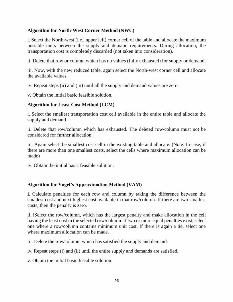
96

Algorithm for North-West Corner Method (NWC)

i. Select the North-west (i.e., upper left) corner cell of the table and allocate the maximum

possible units between the supply and demand requirements. During allocation, the

transportation cost is completely discarded (not taken into consideration).

ii. Delete that row or column which has no values (fully exhausted) for supply or demand.

iii. Now, with the new reduced table, again select the North-west corner cell and allocate

the available values.

iv. Repeat steps (ii) and (iii) until all the supply and demand values are zero.

v. Obtain the initial basic feasible solution.

Algorithm for Least Cost Method (LCM)

i. Select the smallest transportation cost cell available in the entire table and allocate the

supply and demand.

ii. Delete that row/column which has exhausted. The deleted row/column must not be

considered for further allocation.

iii. Again select the smallest cost cell in the existing table and allocate. (Note: In case, if

there are more than one smallest costs, select the cells where maximum allocation can be

made)

iv. Obtain the initial basic feasible solution.

Algorithm for Vogel’s Approximation Method (VAM)

i. Calculate penalties for each row and column by taking the difference between the

smallest cost and next highest cost available in that row/column. If there are two smallest

costs, then the penalty is zero.

ii. iSelect the row/column, which has the largest penalty and make allocation in the cell

having the least cost in the selected row/column. If two or more equal penalties exist, select

one where a row/column contains minimum unit cost. If there is again a tie, select one

where maximum allocation can be made.

iii. Delete the row/column, which has satisfied the supply and demand.

iv. Repeat steps (i) and (ii) until the entire supply and demands are satisfied.

v. Obtain the initial basic feasible solution.

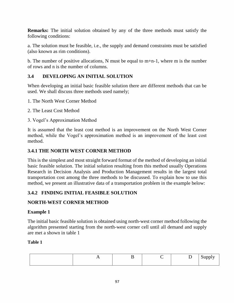
97

Remarks: The initial solution obtained by any of the three methods must satisfy the

following conditions:

a. The solution must be feasible, i.e., the supply and demand constraints must be satisfied

(also known as rim conditions).

b. The number of positive allocations, N must be equal to m+n-1, where m is the number

of rows and n is the number of columns.

3.4 DEVELOPING AN INITIAL SOLUTION

When developing an initial basic feasible solution there are different methods that can be

used. We shall discuss three methods used namely;

1. The North West Corner Method

2. The Least Cost Method

3. Vogel’s Approximation Method

It is assumed that the least cost method is an improvement on the North West Corner

method, while the Vogel’s approximation method is an improvement of the least cost

method.

3.4.1 THE NORTH WEST CORNER METHOD

This is the simplest and most straight forward format of the method of developing an initial

basic feasible solution. The initial solution resulting from this method usually Operations

Research in Decision Analysis and Production Management results in the largest total

transportation cost among the three methods to be discussed. To explain how to use this

method, we present an illustrative data of a transportation problem in the example below:

3.4.2 FINDING INITIAL FEASIBLE SOLUTION

NORTH-WEST CORNER METHOD

Example 1

The initial basic feasible solution is obtained using north-west corner method following the

algorithm presented starting from the north-west corner cell until all demand and supply

are met a shown in table 1

Table 1

A B C D Supply

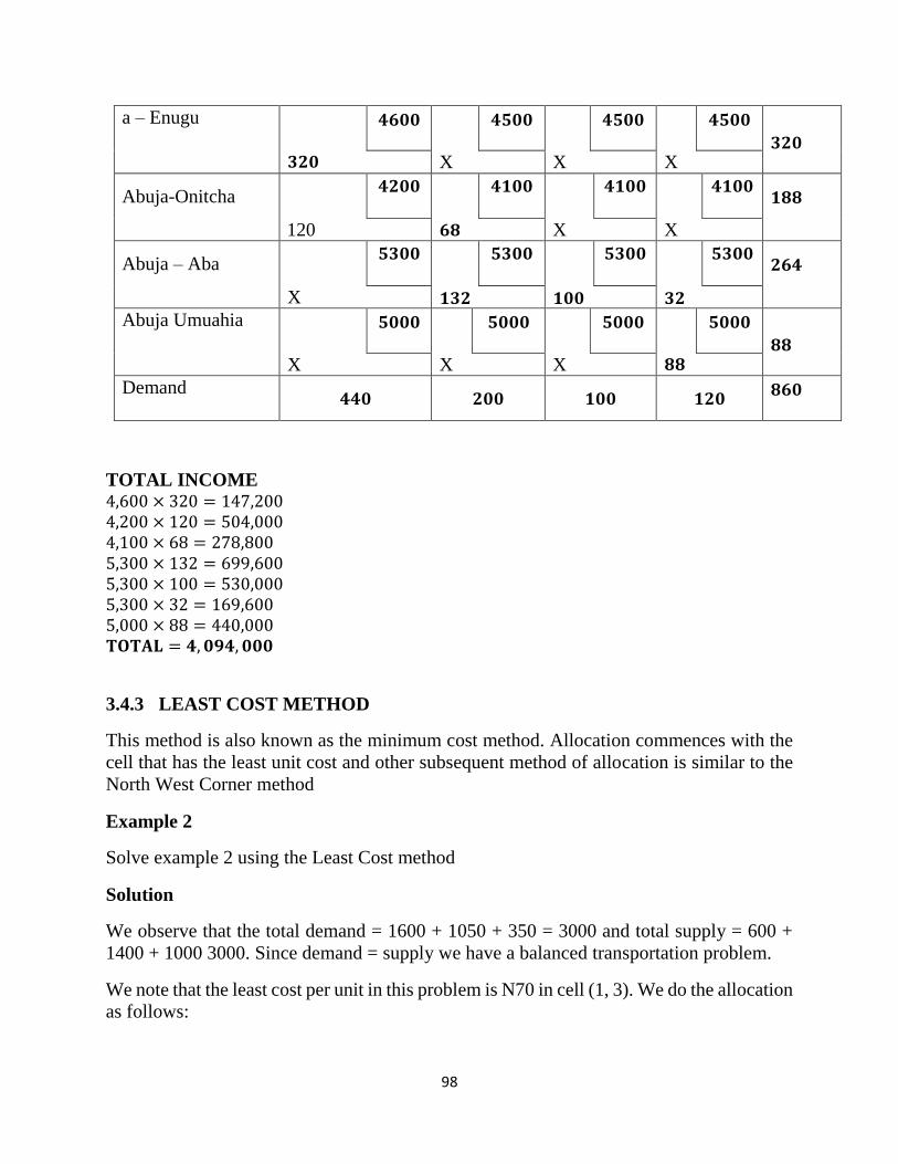
98

a – Enugu 𝟒𝟔𝟎𝟎 𝟒𝟓𝟎𝟎 𝟒𝟓𝟎𝟎 𝟒𝟓𝟎𝟎

𝟑𝟐𝟎 𝟑𝟐𝟎 X X X

Abuja-Onitcha 𝟒𝟐𝟎𝟎 𝟒𝟏𝟎𝟎 𝟒𝟏𝟎𝟎 𝟒𝟏𝟎𝟎

𝟏𝟖𝟖

120 𝟔𝟖 X X

Abuja – Aba 𝟓𝟑𝟎𝟎 𝟓𝟑𝟎𝟎 𝟓𝟑𝟎𝟎 𝟓𝟑𝟎𝟎

𝟐𝟔𝟒

X 𝟏𝟑𝟐 𝟏𝟎𝟎 𝟑𝟐

Abuja Umuahia 𝟓𝟎𝟎𝟎 𝟓𝟎𝟎𝟎 𝟓𝟎𝟎𝟎 𝟓𝟎𝟎𝟎

𝟖𝟖 X X X 𝟖𝟖

Demand 𝟒𝟒𝟎 𝟐𝟎𝟎 𝟏𝟎𝟎 𝟏𝟐𝟎

𝟖𝟔𝟎

TOTAL INCOME 4,600 × 320 = 147,200 4,200 × 120 = 504,000 4,100 × 68 = 278,800 5,300 × 132 = 699,600 5,300 × 100 = 530,000 5,300 × 32 = 169,600 5,000 × 88 = 440,000 𝐓𝐎𝐓𝐀𝐋 = 𝟒, 𝟎𝟗𝟒, 𝟎𝟎𝟎

3.4.3 LEAST COST METHOD

This method is also known as the minimum cost method. Allocation commences with the

cell that has the least unit cost and other subsequent method of allocation is similar to the

North West Corner method

Example 2

Solve example 2 using the Least Cost method

Solution

We observe that the total demand = 1600 + 1050 + 350 = 3000 and total supply = 600 +

1400 + 1000 3000. Since demand = supply we have a balanced transportation problem.

We note that the least cost per unit in this problem is N70 in cell (1, 3). We do the allocation

as follows:

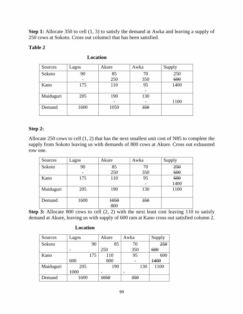
99

Step 1: Allocate 350 to cell (1, 3) to satisfy the demand at Awka and leaving a supply of

250 cows at Sokoto. Cross out column3 that has been satisfied.

Table 2

Location

Sources Lagos Akure Awka Supply

Sokoto 90

-

85

250

70

350

250

600

Kano 175

110

95

-

1400

Maiduguri 205

190

-

130

-

1100

Demand 1600

1050

350

Step 2:

Allocate 250 cows to cell (1, 2) that has the next smallest unit cost of N85 to complete the

supply from Sokoto leaving us with demands of 800 cows at Akure. Cross out exhausted

row one.


Sokoto 90

-

85

250

70

350

250

600

Kano 175

110

95

-

600

1400

Maiduguri 205

190

130

1100

Demand 1600

1050

800

350

Step 3: Allocate 800 cows to cell (2, 2) with the next least cost leaving 110 to satisfy

demand at Akure, leaving us with supply of 600 ram at Kano cross out satisfied column 2.

Location


Sokoto 90

-

85

250

70

350

250

600

Kano 175

600

110

800

95

-

600

1400

Maiduguri 205

1000

190

-

130

-

1100

Demand 1600 1050 350

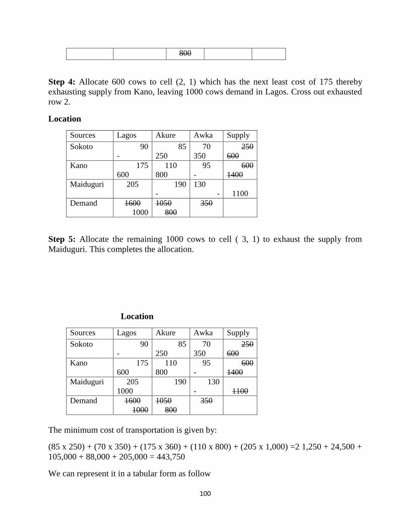
100

800

Step 4: Allocate 600 cows to cell (2, 1) which has the next least cost of 175 thereby

exhausting supply from Kano, leaving 1000 cows demand in Lagos. Cross out exhausted

row 2.

Location


Sokoto 90

-

85

250

70

350

250

600

Kano 175

600

110

800

95

-

600

1400

Maiduguri 205

190

-

130

-

1100

Demand 1600

1000

1050

800

350

Step 5: Allocate the remaining 1000 cows to cell ( 3, 1) to exhaust the supply from

Maiduguri. This completes the allocation.

Location


Sokoto 90

-

85

250

70

350

250

600

Kano 175

600

110

800

95

-

600

1400

Maiduguri 205

1000

190

130

-

1100

Demand 1600

1000

1050

800

350

The minimum cost of transportation is given by:

(85 x 250) + (70 x 350) + (175 x 360) + (110 x 800) + (205 x 1,000) =2 1,250 + 24,500 +

105,000 + 88,000 + 205,000 = 443,750

We can represent it in a tabular form as follow

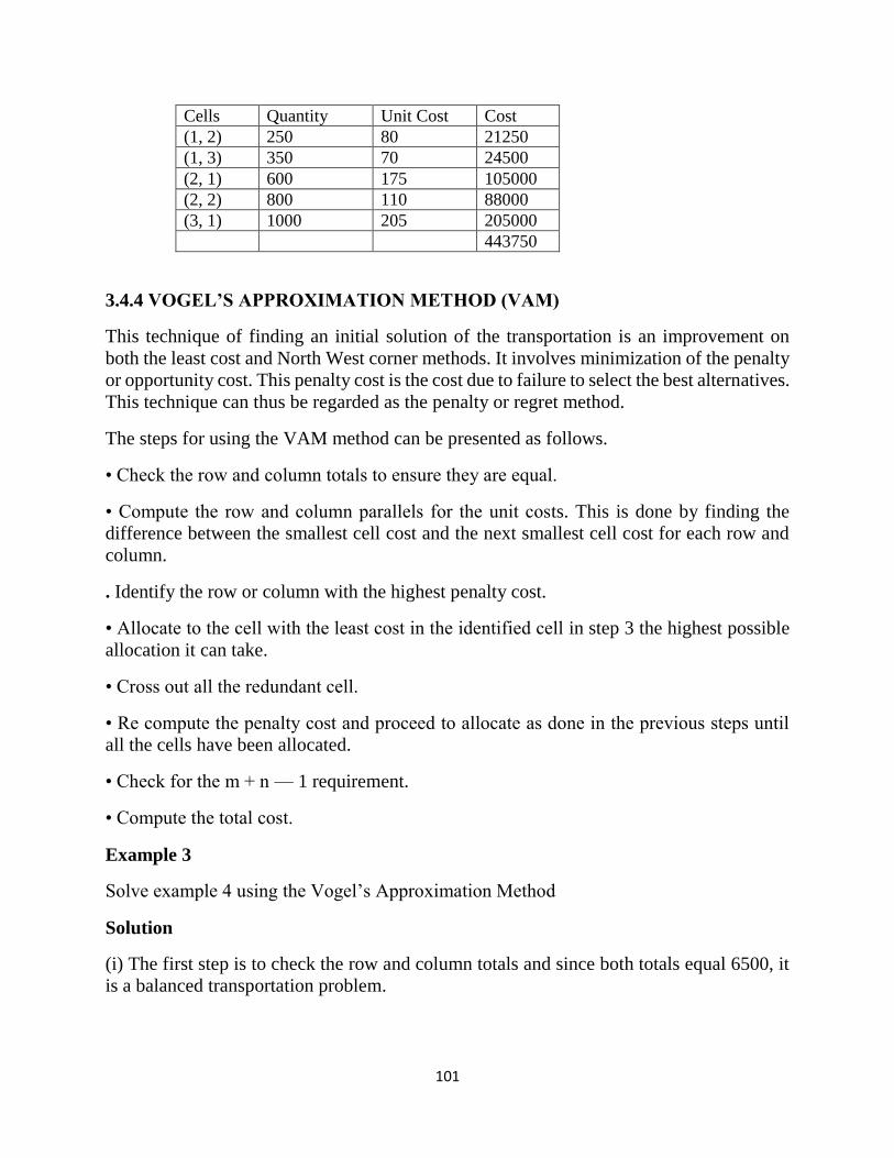
101

Cells Quantity Unit Cost Cost

(1, 2) 250 80 21250

(1, 3) 350 70 24500

(2, 1) 600 175 105000

(2, 2) 800 110 88000

(3, 1) 1000 205 205000

443750

3.4.4 VOGEL’S APPROXIMATION METHOD (VAM)

This technique of finding an initial solution of the transportation is an improvement on

both the least cost and North West corner methods. It involves minimization of the penalty

or opportunity cost. This penalty cost is the cost due to failure to select the best alternatives.

This technique can thus be regarded as the penalty or regret method.

The steps for using the VAM method can be presented as follows.

• Check the row and column totals to ensure they are equal.

• Compute the row and column parallels for the unit costs. This is done by finding the

difference between the smallest cell cost and the next smallest cell cost for each row and

column.

. Identify the row or column with the highest penalty cost.

• Allocate to the cell with the least cost in the identified cell in step 3 the highest possible

allocation it can take.

• Cross out all the redundant cell.

• Re compute the penalty cost and proceed to allocate as done in the previous steps until

all the cells have been allocated.

• Check for the m + n — 1 requirement.

• Compute the total cost.

Example 3

Solve example 4 using the Vogel’s Approximation Method

Solution

(i) The first step is to check the row and column totals and since both totals equal 6500, it

is a balanced transportation problem.

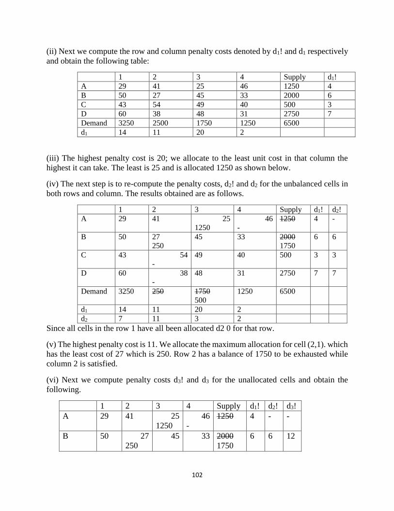
102

(ii) Next we compute the row and column penalty costs denoted by d1! and d1 respectively

and obtain the following table:

1 2 3 4 Supply d1!

A 29 41 25 46 1250 4

B 50 27 45 33 2000 6

C 43 54 49 40 500 3

D 60 38 48 31 2750 7

Demand 3250 2500 1750 1250 6500

d1 14 11 20 2

(iii) The highest penalty cost is 20; we allocate to the least unit cost in that column the

highest it can take. The least is 25 and is allocated 1250 as shown below.

(iv) The next step is to re-compute the penalty costs, d2! and d2 for the unbalanced cells in

both rows and column. The results obtained are as follows.

1 2 3 4 Supply d1! d2!

A 29 41 25

1250

46

-

1250 4 -

B 50 27

250

45 33 2000

1750

6 6

C 43 54

-

49 40 500 3 3

D 60 38

-

48 31 2750 7 7

Demand 3250 250 1750

500

1250 6500

d1 14 11 20 2

d2 7 11 3 2

Since all cells in the row 1 have all been allocated d2 0 for that row.

(v) The highest penalty cost is 11. We allocate the maximum allocation for cell (2,1). which

has the least cost of 27 which is 250. Row 2 has a balance of 1750 to be exhausted while

column 2 is satisfied.

(vi) Next we compute penalty costs d3! and d3 for the unallocated cells and obtain the

following.

1 2 3 4 Supply d1! d2! d3!

A 29 41 25

1250

46

-

1250 4 - -

B 50 27

250

45 33 2000

1750

6 6 12

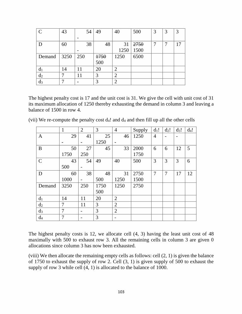
103

C 43 54

-

49 40 500 3 3 3

D 60 38

-

48 31

1250

2750

1500

7 7 17

Demand 3250 250 1750

500

1250 6500

d1 14 11 20 2

d2 7 11 3 2

d3 7 - 3 2

The highest penalty cost is 17 and the unit cost is 31. We give the cell with unit cost of 31

its maximum allocation of 1250 thereby exhausting the demand in column 3 and leaving a

balance of 1500 in row 4.

(vii) We re-compute the penalty cost d4! and d4 and then fill up all the other cells

1 2 3 4 Supply d1! d2! d3! d4!

A 29

-

41

-

25

1250

46

-

1250 4 - -

B 50

1750

27

250

45 33 2000

1750

6 6 12 5

C 43

500

54

-

49 40 500 3 3 3 6

D 60

1000

38

-

48

500

31

1250

2750

1500

7 7 17 12

Demand 3250 250 1750

500

1250 2750

d1 14 11 20 2

d2 7 11 3 2

d3 7 - 3 2

d4 7 - 3 -

The highest penalty costs is 12, we allocate cell (4, 3) having the least unit cost of 48

maximally with 500 to exhaust row 3. All the remaining cells in column 3 are given 0

allocations since column 3 has now been exhausted.

(viii) We then allocate the remaining empty cells as follows: cell (2, 1) is given the balance

of 1750 to exhaust the supply of row 2. Cell (3, 1) is given supply of 500 to exhaust the

supply of row 3 while cell (4, 1) is allocated to the balance of 1000.

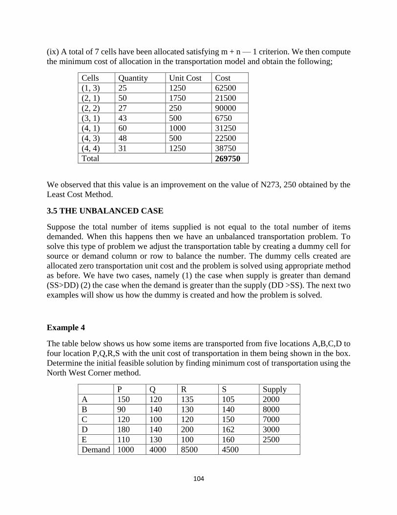
104

(ix) A total of 7 cells have been allocated satisfying m + n — 1 criterion. We then compute

the minimum cost of allocation in the transportation model and obtain the following;


(1, 3) 25 1250 62500

(2, 1) 50 1750 21500

(2, 2) 27 250 90000

(3, 1) 43 500 6750

(4, 1) 60 1000 31250

(4, 3) 48 500 22500

(4, 4) 31 1250 38750

Total 269750

We observed that this value is an improvement on the value of N273, 250 obtained by the

Least Cost Method.

3.5 THE UNBALANCED CASE

Suppose the total number of items supplied is not equal to the total number of items

demanded. When this happens then we have an unbalanced transportation problem. To

solve this type of problem we adjust the transportation table by creating a dummy cell for

source or demand column or row to balance the number. The dummy cells created are

allocated zero transportation unit cost and the problem is solved using appropriate method

as before. We have two cases, namely (1) the case when supply is greater than demand

(SS>DD) (2) the case when the demand is greater than the supply (DD >SS). The next two

examples will show us how the dummy is created and how the problem is solved.

Example 4

The table below shows us how some items are transported from five locations A,B,C,D to

four location P,Q,R,S with the unit cost of transportation in them being shown in the box.

Determine the initial feasible solution by finding minimum cost of transportation using the

North West Corner method.

P Q R S Supply

A 150 120 135 105 2000

B 90 140 130 140 8000

C 120 100 120 150 7000

D 180 140 200 162 3000

E 110 130 100 160 2500

Demand 1000 4000 8500 4500

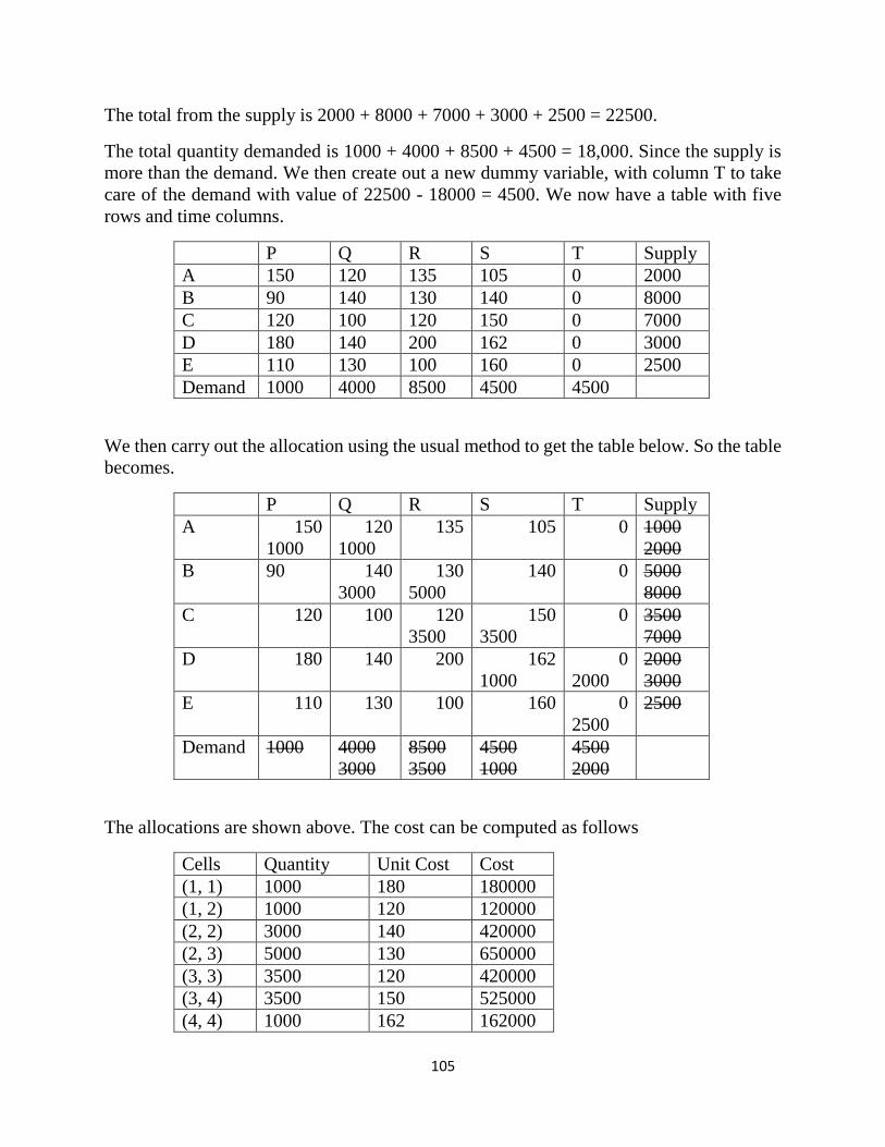
105

The total from the supply is 2000 + 8000 + 7000 + 3000 + 2500 = 22500.

The total quantity demanded is 1000 + 4000 + 8500 + 4500 = 18,000. Since the supply is

more than the demand. We then create out a new dummy variable, with column T to take

care of the demand with value of 22500 - 18000 = 4500. We now have a table with five

rows and time columns.

P Q R S T Supply

A 150 120 135 105 0 2000

B 90 140 130 140 0 8000

C 120 100 120 150 0 7000

D 180 140 200 162 0 3000

E 110 130 100 160 0 2500

Demand 1000 4000 8500 4500 4500

We then carry out the allocation using the usual method to get the table below. So the table

becomes.

P Q R S T Supply

A 150

1000

120

1000

135 105 0 1000

2000

B 90

140

3000

130

5000

140 0 5000

8000

C 120

100 120

3500

150

3500

0 3500

7000

D 180

140 200 162

1000

0

2000

2000

3000

E 110 130 100 160 0

2500

2500

Demand 1000 4000

3000

8500

3500

4500

1000

4500

2000

The allocations are shown above. The cost can be computed as follows


(1, 1) 1000 180 180000

(1, 2) 1000 120 120000

(2, 2) 3000 140 420000

(2, 3) 5000 130 650000

(3, 3) 3500 120 420000

(3, 4) 3500 150 525000

(4, 4) 1000 162 162000

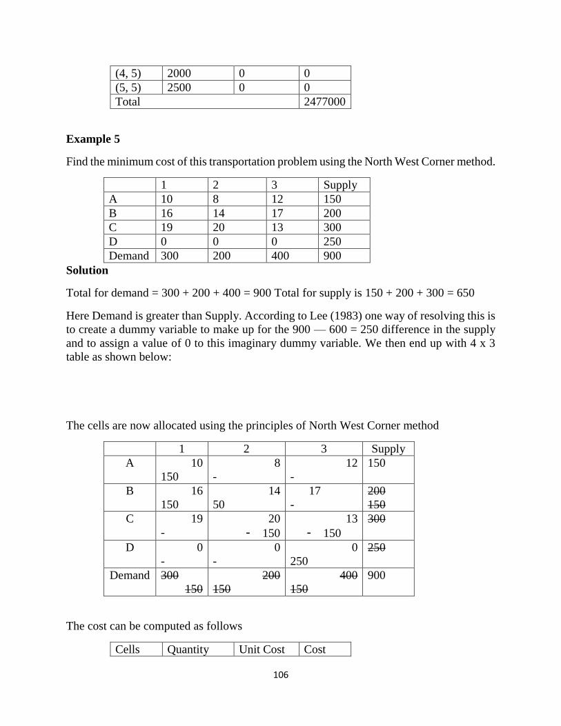
106

(4, 5) 2000 0 0

(5, 5) 2500 0 0

Total 2477000

Example 5

Find the minimum cost of this transportation problem using the North West Corner method.

1 2 3 Supply

A 10 8 12 150

B 16 14 17 200

C 19 20 13 300

D 0 0 0 250

Demand 300 200 400 900

Solution

Total for demand = 300 + 200 + 400 = 900 Total for supply is 150 + 200 + 300 = 650

Here Demand is greater than Supply. According to Lee (1983) one way of resolving this is

to create a dummy variable to make up for the 900 — 600 = 250 difference in the supply

and to assign a value of 0 to this imaginary dummy variable. We then end up with 4 x 3

table as shown below:

The cells are now allocated using the principles of North West Corner method

1 2 3 Supply

A 10

150

8

-

12

-

150

B 16

150

14

50

17

-

200

150

C 19

-

20

- 150

13

- 150

300

D 0

-

0

-

0

250

250

Demand 300

150

200

150

400

150

900

The cost can be computed as follows


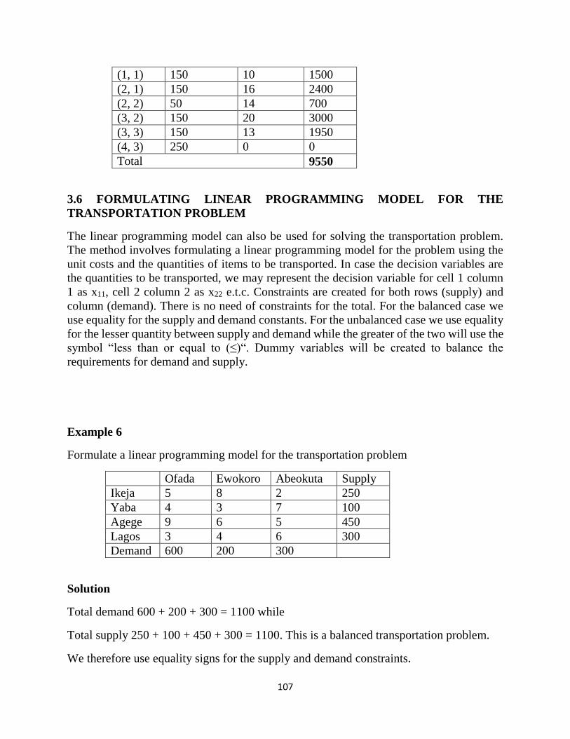
107

(1, 1) 150 10 1500

(2, 1) 150 16 2400

(2, 2) 50 14 700

(3, 2) 150 20 3000

(3, 3) 150 13 1950

(4, 3) 250 0 0

Total 9550

3.6 FORMULATING LINEAR PROGRAMMING MODEL FOR THE

TRANSPORTATION PROBLEM

The linear programming model can also be used for solving the transportation problem.

The method involves formulating a linear programming model for the problem using the

unit costs and the quantities of items to be transported. In case the decision variables are

the quantities to be transported, we may represent the decision variable for cell 1 column

1 as x11, cell 2 column 2 as x22 e.t.c. Constraints are created for both rows (supply) and

column (demand). There is no need of constraints for the total. For the balanced case we

use equality for the supply and demand constants. For the unbalanced case we use equality

for the lesser quantity between supply and demand while the greater of the two will use the

symbol “less than or equal to (≤)“. Dummy variables will be created to balance the

requirements for demand and supply.

Example 6

Formulate a linear programming model for the transportation problem

Ofada Ewokoro Abeokuta Supply

Ikeja 5 8 2 250

Yaba 4 3 7 100

Agege 9 6 5 450

Lagos 3 4 6 300

Demand 600 200 300

Solution

Total demand 600 + 200 + 300 = 1100 while

Total supply 250 + 100 + 450 + 300 = 1100. This is a balanced transportation problem.

We therefore use equality signs for the supply and demand constraints.

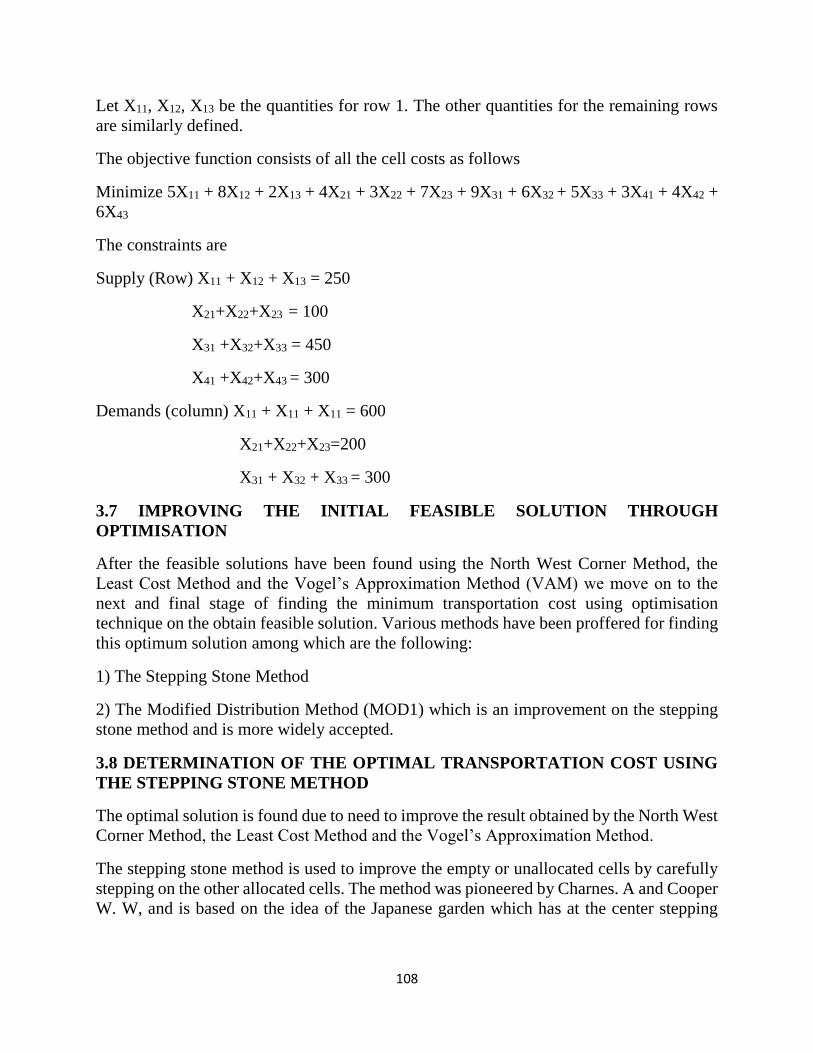
108

Let X11, X12, X13 be the quantities for row 1. The other quantities for the remaining rows

are similarly defined.

The objective function consists of all the cell costs as follows

Minimize 5X11 + 8X12 + 2X13 + 4X21 + 3X22 + 7X23 + 9X31 + 6X32 + 5X33 + 3X41 + 4X42 +

6X43

The constraints are

Supply (Row) X11 + X12 + X13 = 250

X21+X22+X23 = 100

X31 +X32+X33 = 450

X41 +X42+X43 = 300

Demands (column) X11 + X11 + X11 = 600

X21+X22+X23=200

X31 + X32 + X33 = 300

3.7 IMPROVING THE INITIAL FEASIBLE SOLUTION THROUGH

OPTIMISATION

After the feasible solutions have been found using the North West Corner Method, the

Least Cost Method and the Vogel’s Approximation Method (VAM) we move on to the

next and final stage of finding the minimum transportation cost using optimisation

technique on the obtain feasible solution. Various methods have been proffered for finding

this optimum solution among which are the following:

1) The Stepping Stone Method

2) The Modified Distribution Method (MOD1) which is an improvement on the stepping

stone method and is more widely accepted.

3.8 DETERMINATION OF THE OPTIMAL TRANSPORTATION COST USING

THE STEPPING STONE METHOD

The optimal solution is found due to need to improve the result obtained by the North West

Corner Method, the Least Cost Method and the Vogel’s Approximation Method.

The stepping stone method is used to improve the empty or unallocated cells by carefully

stepping on the other allocated cells. The method was pioneered by Charnes. A and Cooper

W. W, and is based on the idea of the Japanese garden which has at the center stepping

109

stones carefully laid across the path which enables one to cross the path by stepping

carefully on the stones.

The criterion of m + n - 1 number of occupied cells must be satisfied to avoid degeneracy.

The stepping stone method is similar to the simplex method in the sense that occupied cells

are the basic variables of the simplex method while the empty cells are the non-basic

variables. To find the optimum solution we assess a stepping stone path by stepping on

allocated cells in order to evaluate an empty cell. The set of allocated cells that must be

stepped on in order to evaluate an unallocated cell is known as the stepping stone path. It

is identical to the positive or negative variables on a non-basic column of the simplex

tableau. The critical thing to do is to find the stepping stone path in order to find out the

net change in transportation by re-allocation of cells. In re-allocating cells it is very

important that the total supply and total demand is kept constant.

The following steps are essential in using the stepping stone method:

• Identify the stepping stone path for all the unallocated cells.

• Trace the stepping stone paths to identify if transportation of one unit will incur a

difference in total transportation cost. One may need to skip an empty cell or even an

occupied cell when tracing the path. We usually represent increase with a positive sign and

a decrease with negative sign.

• Using the traced stepping stone paths analyze the unit transportation cost in each cell.

Compute the Cost Improvement Index (CII) for each empty cell.

• Select the cell with the largest negative CII for allocation, bearing in mind the need to

ensure that the demand and supply are both kept constant and calculate the cost of

transportation. Re-compute the CII for the new table. if all the CIls are positive then we

have reached the optimum allocation otherwise the procedure is iterated until we get

positive values for all the CIIs in the transportation table.

The following points should be noted when using the stepping stone method:

• It will be observed that if iteration is necessary the transportation cost in cacti of the

subsequent table will reduce until we obtain the optimum solution.

• Only sources transport goods to destinations. Re-allocation is done using horizontal

movements for rows and vertical movement columns.

• Every empty cell has a unique stepping stone path.

• The stepping stone path consists of allocated cells.

Example 7

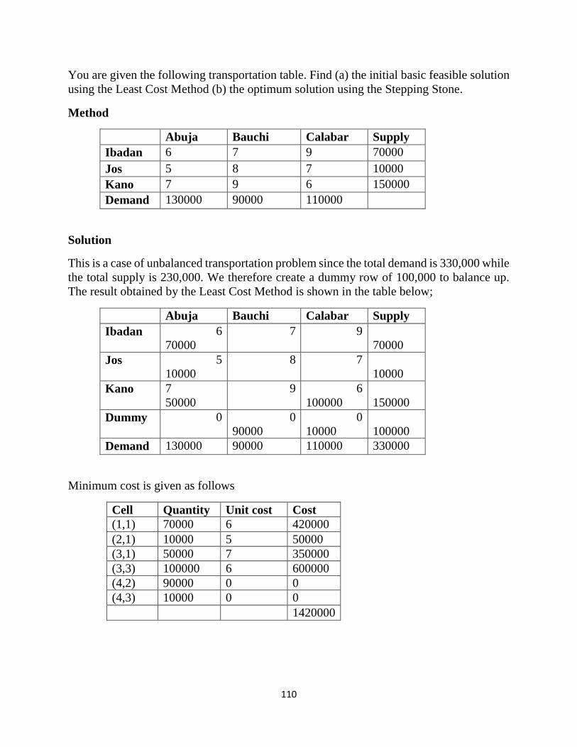
110

You are given the following transportation table. Find (a) the initial basic feasible solution

using the Least Cost Method (b) the optimum solution using the Stepping Stone.

Method

Abuja Bauchi Calabar Supply

Ibadan 6 7 9 70000

Jos 5 8 7 10000

Kano 7 9 6 150000

Demand 130000 90000 110000

Solution

This is a case of unbalanced transportation problem since the total demand is 330,000 while

the total supply is 230,000. We therefore create a dummy row of 100,000 to balance up.

The result obtained by the Least Cost Method is shown in the table below;


Ibadan 6

70000

7 9

70000

Jos 5

10000

8 7

10000

Kano 7

50000

9 6

100000

150000

Dummy 0 0

90000

0

10000

100000

Demand 130000 90000 110000 330000

Minimum cost is given as follows

Cell Quantity Unit cost Cost

(1,1) 70000 6 420000

(2,1) 10000 5 50000

(3,1) 50000 7 350000

(3,3) 100000 6 600000

(4,2) 90000 0 0

(4,3) 10000 0 0

1420000

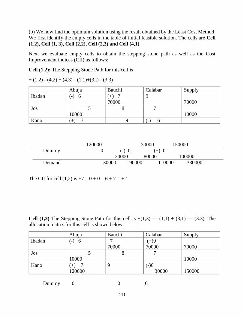
111

(b) We now find the optimum solution using the result obtained by the Least Cost Method.

We first identify the empty cells in the table of initial feasible solution. The cells are Cell

(1,2), Cell (1, 3), Cell (2,2), Cell (2,3) and Cell (4,1)

Next we evaluate empty cells to obtain the stepping stone path as well as the Cost

Improvement indices (CII) as follows:

Cell (1,2): The Stepping Stone Path for this cell is

+ (1,2) - (4,2) + (4,3) - (1,1)+(3,l) - (3,3)


Ibadan (-) 6 (+) 7

70000

9

70000

Jos 5

10000

8 7

10000

Kano (+) 7 9 (-) 6

120000 30000 150000

Dummy 0 (-) 0 (+) 0

20000 80000 100000

Demand 130000 90000 110000 330000

The CII for cell (1,2) is +7 – 0 + 0 – 6 + 7 = +2

Cell (1,3) The Stepping Stone Path for this cell is +(1,3) — (1,1) + (3,1) — (3.3). The

allocation matrix for this cell is shown below:


Ibadan (-) 6 7

70000

(+)9

70000

70000

Jos 5

10000

8 7

10000

Kano (+) 7

120000

9 (-)6

30000

150000

Dummy 0 0 0

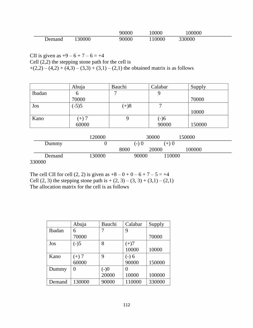
112

90000 10000 100000

Demand 130000 90000 110000 330000

CII is given as +9 – 6 + 7 – 6 = +4

Cell (2,2) the stepping stone path for the cell is

+(2,2) – (4,2) + (4,3) – (3,3) + (3,1) – (2,1) the obtained matrix is as follows


Ibadan 6

70000

7

9

70000

Jos (-5)5

(+)8 7

10000

Kano (+) 7

60000

9 (-)6

90000

150000

120000 30000 150000

Dummy 0 (-) 0 (+) 0

8000 20000 100000

Demand 130000 90000 110000

330000

The cell CII for cell (2, 2) is given as +8 – 0 + 0 – 6 + 7 – 5 = +4

Cell (2, 3) the stepping stone path is + (2, 3) – (3, 3) + (3,1) – (2,1)

The allocation matrix for the cell is as follows


Ibadan 6

70000

7 9

70000

Jos (-)5 8 (+)7

10000

10000

Kano (+) 7

60000

9 (-) 6

90000

150000

Dummy 0 (-)0

20000

0

10000

100000

Demand 130000 90000 110000 330000

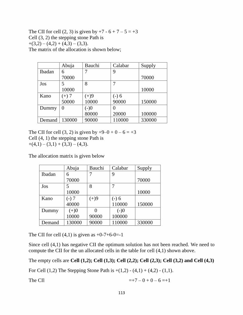
113

The CII for cell (2, 3) is given by +7 - 6 + 7 – 5 = +3

Cell (3, 2) the stepping stone Path is

+(3,2) – (4,2) + (4,3) – (3,3).

The matrix of the allocation is shown below;


Ibadan 6

70000

7 9

70000

Jos 5

10000

8 7

10000

Kano (+) 7

50000

(+)9

10000

(-) 6

90000

150000

Dummy 0 (-)0

80000

0

20000

100000

Demand 130000 90000 110000 330000

The CII for cell (3, 2) is given by +9–0 + 0 – 6 = +3

Cell (4, 1) the stepping stone Path is

+(4,1) – (3,1) + (3,3) – (4,3).

The allocation matrix is given below


Ibadan 6

70000

7 9

70000

Jos 5

10000

8 7

10000

Kano (-) 7

40000

(+)9

(-) 6

110000

150000

Dummy (+)0

10000

0

90000

(-)0

100000

Demand 130000 90000 110000 330000

The CII for cell (4,1) is given as +0-7+6-0=-1

Since cell (4,1) has negative CII the optimum solution has not been reached. We need to

compute the CII for the un allocated cells in the table for cell (4,1) shown above.

The empty cells are Cell (1,2); Cell (1,3); Cell (2,2); Cell (2,3); Cell (3,2) and Cell (4,3)

For Cell (1,2) The Stepping Stone Path is +(1,2) - (4,1) + (4,2) - (1,1).

The CIl =+7 – 0 + 0 – 6 =+1

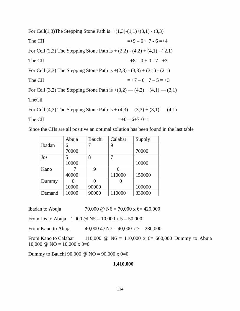
114

For Cell(1,3)The Stepping Stone Path is +(1,3)-(1,1)+(3,1) - (3,3)

The CII =+9 – 6 + 7 - 6 =+4

For Cell (2,2) The Stepping Stone Path is + (2,2) - (4,2) + (4,1) - ( 2,1)

The CIl =+8 – 0 + 0 - 7= +3

For Cell (2,3) The Stepping Stone Path is +(2,3) - (3,3) + (3,1) - (2,1)

The CIl = +7 – 6 +7 – 5 = +3

For Cell (3,2) The Stepping Stone Path is +(3,2) — (4,2) + (4,1) — (3,1)

TheCil

For Cell (4,3) The Stepping Stone Path is + (4,3)— (3,3) + (3,1) — (4,1)

The CIl =+0—6+7-0=1

Since the CIIs are all positive an optimal solution has been found in the last table


Ibadan 6

70000

7 9

70000

Jos 5

10000

8 7

10000

Kano 7

40000

9

6

110000

150000

Dummy 0

10000

0

90000

0

100000

Demand 10000 90000 110000 330000

Ibadan to Abuja 70,000 @ N6 = 70,000 x 6= 420,000

From Jos to Abuja 1,000 @ N5 = 10,000 x 5 = 50,000

From Kano to Abuja 40,000 @ N7 = 40,000 x 7 = 280,000

From Kano to Calabar 110,000 @ N6 = 110,000 x 6= 660,000 Dummy to Abuja

10,000 @ NO = 10,000 x 0=0

Dummy to Bauchi 90,000 @ NO = 90,000 x 0=0

1,410,000

115

We observe that the minimum cost of 1, 420, 000 obtained by the Least Cost Method has

been reduced by the stepping stone method to give s the optimum transportation cost of

1,410, 000.

3.9 THE MODIFIED DISTRIBUTION METHOD

This method is usually applied to the initial feasible solution obtained by the North West

Corner method and the Least Cost method since the initial feasible solution obtained by

the Vogel’s Approximation Method, is deemed to be more accurate than these two. To use

this method we take the following steps:

Step 1: Using the obtained feasible solution, compute the row dispatch unit cost r1 and the

column reception unit cost cij at location j for every cell with allocation using

Cij = ri+cj

Conventionally, ri = 0

Note that ri is the shadow cost of dispatching a unit item from source to cell kij while cj is

the shadow cost of receiving a unit of the item from location j to cell kij and cij is the cost

of transporting a unit of the item from source i to location j in the corresponding cell kij.

If we have a 3 x 3 cell we obtain r1, r2, r3, c1,c2, and c3 respectively.

Step 2

Compute the unit shadow costs for each of the empty unallocated cells using the various

obtained ci and ri

Step 3

Obtain the differences in unit costs for the unallocated cells using

C1ij =cij- (ri+cj)

If these differences are all positive for the empty cells the minimum optimum solution has

been obtained. If we have one or more records of any negative difference then it implies

that an improved solution can still be obtained and so we proceed to step 4.

Step 4

We select the cell with the highest negative value of Cij. If more than one of them have the

same negative Cij (i.e. the unit shadow cost is greater than the actual cost), that is a tie

occurs we select any one of them arbitrarily for transfer of units.

Step 5 Transfer to the empty cells the minimum value possible from an allocated cell, taking care

that the values of the demand and supply are unaffected by the transfer and that no other

empty cell is given allocation.

116

Step 6

Develop a new solution and test if it is the optimum solution

Step 7

If it is not, repeat the procedures by starting from step 1 until the optimum solution is

obtained.

Example 8

In the transportation table given below:

(a) Find the initial feasible solution using (i) the least cost method (ii) the Vogel’s

approximation method.

Use the modified Distribution method to find the optimum solution using the initial feasible

solution obtained by the Least Cost Method.

1 2 3 Supply

X 9 11 15 400

Y 15 7 17 500

Z 11 5 7 600

Demand 500 450 550

Solution

We use the least cost method to obtain this table

1 2 3 Supply

X 9 11 15

400 - - 400

Y 15 7 17

100 - 400 500

Z 11 5 7

- 450 150 600

Demand 500 450 550

The Least Cost value is (400 x 9) + (100 x 15) + (450 x 5) + (400 x 17) + (550 x 7)

= 3600+1500+2250+6800+1050= 15200

Minimum cost by least cost = 15200

ii. Using the Vogel approximation method,

X Y Z Supply d1 d2 d3

A 9

400

11

-

15

-

400

2

6

6*

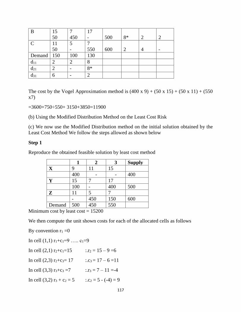
117

B 15

50

7

450

17

-

500

8*

2

2

C 11

50

5

-

7

550

600

2

4

-

Demand 150 100 130

d11 2 2 8

d21 2 - 8*

d31 6 - 2

The cost by the Vogel Approximation method is (400 x 9) + (50 x 15) + (50 x 11) + (550

x7)

=3600+750÷550+ 3150+3850=11900

(b) Using the Modified Distribution Method on the Least Cost Risk

(c) We now use the Modified Distribution method on the initial solution obtained by the

Least Cost Method We follow the steps allowed as shown below

Step 1

Reproduce the obtained feasible solution by least cost method

1 2 3 Supply

X 9 11 15

400 - - 400

Y 15 7 17

100 - 400 500

Z 11 5 7

- 450 150 600

Demand 500 450 550

Minimum cost by least cost = 15200

We then compute the unit shown costs for each of the allocated cells as follows

By convention r1 =0

In cell (1,1) r1+c1=9 ….. c1=9

In cell (2,1) r2+c1=15 :.r2 = 15 – 9 =6

In cell (2,3) r2+c3= 17 :.c3 = 17 – 6 =11

In cell (3,3) r3+c3 =7 :.r3 = 7 – 11 =-4

In cell (3,2) r3 + c2 = 5 :.c2 = 5 - (-4) = 9

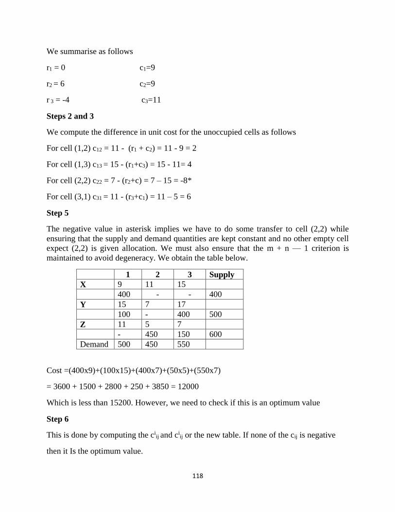
118

We summarise as follows

r1 = 0 c1=9

r2 = 6 c2=9

r 3 = -4 c3=11

Steps 2 and 3

We compute the difference in unit cost for the unoccupied cells as follows

For cell (1,2) c12 = 11 - (r1 + c2) = 11 - 9 = 2

For cell (1,3) c13 = 15 - (r1+c3) = 15 - 11= 4

For cell (2,2) c22 = 7 - (r2+c) = 7 – 15 = -8*

For cell (3,1) c31 = 11 - (r3+c1) = 11 – 5 = 6

Step 5

The negative value in asterisk implies we have to do some transfer to cell (2,2) while

ensuring that the supply and demand quantities are kept constant and no other empty cell

expect (2,2) is given allocation. We must also ensure that the m + n — 1 criterion is

maintained to avoid degeneracy. We obtain the table below.

1 2 3 Supply

X 9 11 15

400 - - 400

Y 15 7 17

100 - 400 500

Z 11 5 7

- 450 150 600

Demand 500 450 550

Cost =(400x9)+(100x15)+(400x7)+(50x5)+(550x7)

= 3600 + 1500 + 2800 + 250 + 3850 = 12000

Which is less than 15200. However, we need to check if this is an optimum value

Step 6

This is done by computing the ciij and ci

ij or the new table. If none of the cij is negative

then it Is the optimum value.

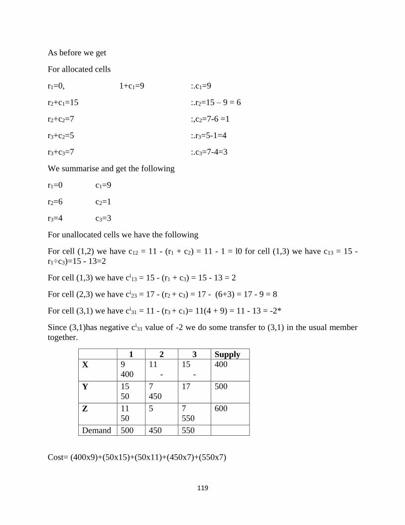
119

As before we get

For allocated cells

r1=0, 1+c1=9 :.c1=9

r2+c1=15 :.r2=15 – 9 = 6

r2+c2=7 :,c2=7-6 =1

r3+c2=5 :.r3=5-1=4

r3+c3=7 :.c3=7-4=3

We summarise and get the following

r1=0 c1=9

r2=6 c2=1

r3=4 c3=3

For unallocated cells we have the following

For cell (1,2) we have c12 = 11 - (r1 + c2) = 11 - 1 = l0 for cell (1,3) we have c13 = 15 -

r1÷c3)=15 - 13=2

For cell (1,3) we have ci13 = 15 - (r1 + c3) = 15 - 13 = 2

For cell (2,3) we have ci23 = 17 - (r2 + c3) = 17 - (6+3) = 17 - 9 = 8

For cell (3,1) we have ci31 = 11 - (r3 + c1)= 11(4 + 9) = 11 - 13 = -2*

Since (3,1)has negative ci31 value of -2 we do some transfer to (3,1) in the usual member

together.

1 2 3 Supply

X 9

400

11

-

15

-

400

Y 15

50

7

450

17

500

Z 11

50

5

7

550

600

Demand 500 450 550

Cost= (400x9)+(50x15)+(50x11)+(450x7)+(550x7)

120

=3600+70+550+3150+3850= 11,900

We check if this is the optimum solution by computing the differences in the unit costs an

unit shadow costs cij in the usual way.

For allocated cells

r1=0, 1+c1 = 9 .: c1 = 9

r2 + c1 = 15 .: r2 = 15 – 9 = 6

r2 + c2 = 7 .: c2 = 7 – 6 = 1

r3+c1= l1 .: r3 = 11 – 9 = 2

r3+c3 = 7 .: c3 = 7 – r3 = 7 – 2 = 5

We summarize and get

r1= 0 c1=9

r2=6 c2=1

r3=2 c3=5

For unallocated cells

(1,2) we have c12 = 11 - (0+1) = 10

for(1,3)we have c13 =15 - (0+5)=10

for (2,3) we have c23=17 - (6+5)=6

for cell (3,2) we have c32 = 5 - (2 + 1) = 2

Since all these values are positive then the last table is the optimum assignment.

The optimum assignment is thus

1 2 3 Supply

X 400 -

-

400

Y 50 450 -

500

Z 50 -

550

600

Demand 500 450 550

The optimum cost is N11,900

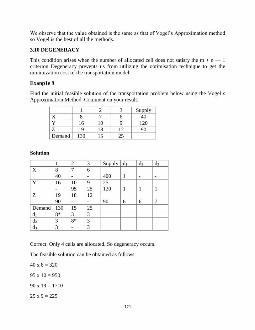
121

We observe that the value obtained is the same as that of Vogel’s Approximation method

so Vogel is the best of all the methods.

3.10 DEGENERACY

This condition arises when the number of allocated cell does not satisfy the m + n — 1

criterion Degeneracy prevents us from utilizing the optimisation technique to get the

minimization cost of the transportation model.

Exanp1e 9

Find the initial feasible solution of the transportation problem below using the Vogel s

Approximation Method. Comment on your result.

1 2 3 Supply

X 8 7 6 40

Y 16 10 9 120

Z 19 18 12 90

Demand 130 15 25

Solution

1 2 3 Supply d1 d2 d3

X 8

40

7

-

6

-

400

1

-

-

Y 16

-

10

95

9

25

25

120

1

1

1

Z 19

90

18

-

12

-

90

6

6

7

Demand 130 15 25

d1 8* 3 3

d2 3 8* 3

d3 3 - 3

Correct: Only 4 cells are allocated. So degeneracy occurs.

The feasible solution can be obtained as follows

40 x 8 = 320

95 x 10 = 950

90 x 19 = 1710

25 x 9 = 225

122

N3,205

Let us compute the shadow costs

By convention r1 = 0

r1+c1 = 8 .: r1 = 8

r2+c2 = l0

r2+c3 = 9

r3+c1=19 :r3=19 – 8 =11

Due to degeneracy we cannot get enough information to enable us calculate r+, c+ and c3.

This implies that we cannot determine the needed row and column values for the

unallocated cells.

The way out is to create a dummy allocated cell which is assigned a value of 0. Others

advocate adding a small value to an empty cell and then proceeding with using MODI to

obtain the optimum solution in the usual way.

4.0 CONCLUSION

The transportation technique was first started in 1941 when Hitchcock published his study

entitled “The distribution of a product from several sources to numerous locations”. Since

then other researchers have developed various techniques of solving the transportation

model. There have been many variants of the transportation model among which is the

assignment method, location — allocation problem and distribution problem. The

transportation method has diverse application in various facets of life. It is applicable in

transporting petroleum products from refinery (sources) to various fuel deports (locations).

5.0 SUMMARY

The transportation model deals with a special class of linear programming problem in

which the objective is to transport a homogeneous commodity from various origins or

factories to different destinations or markets at a total minimum cost. In this unit, we

discussed the following issues- assumptions of the transportation model which include

the Homogeneity of materials to be transported, equality of transportation cost per unit,

uniqueness of route or mode of transportation between each source and destination. It also

discussed extensively, various methods of solving the transportation problem viz: the

North West corner method, the least cost method, Vogel’s approximation method (VAM),

the unbalanced case, formulating linear programming model for the transportation

problem, and determination of the optimal transportation cost using the stepping stone

method.

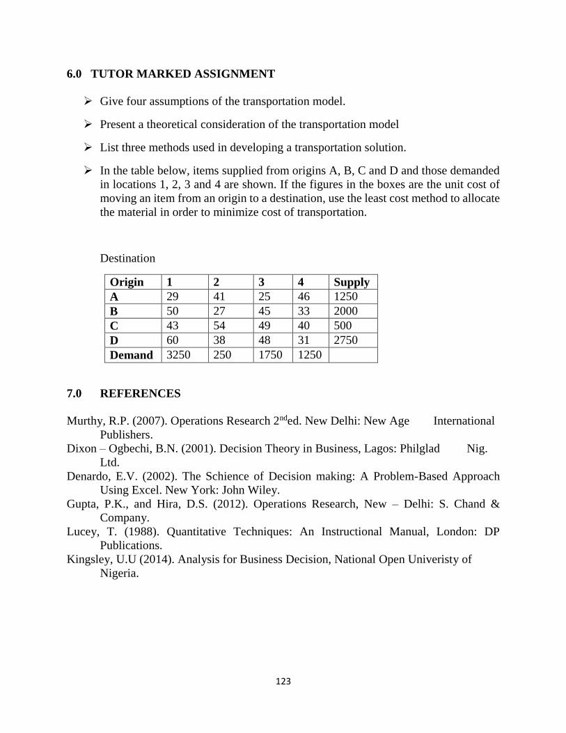
123


Give four assumptions of the transportation model.

Present a theoretical consideration of the transportation model

List three methods used in developing a transportation solution.

In the table below, items supplied from origins A, B, C and D and those demanded

in locations 1, 2, 3 and 4 are shown. If the figures in the boxes are the unit cost of

moving an item from an origin to a destination, use the least cost method to allocate

the material in order to minimize cost of transportation.

Destination

Origin 1 2 3 4 Supply

A 29 41 25 46 1250

B 50 27 45 33 2000

C 43 54 49 40 500

D 60 38 48 31 2750

Demand 3250 250 1750 1250

7.0 REFERENCES

Murthy, R.P. (2007). Operations Research 2nded. New Delhi: New Age International

Publishers.


Ltd.




Company.


Publications.


Nigeria.

124

UNIT 11: ASSIGNMENT MODEL

1.0 Introduction

2.0 Objectives

3.0 Main Content

3.1 The Problem

3.2 Comparison between Transportation Problem and Assignment Problem

3.3 Approach to Solution

4.0 Conclusion

5.0 Summary


7.0 References

125

1.0 INTRODUCTION

Basically assignment model is a minimization model. If we want to maximize the objective

function, then there are two methods. One is to subtract all the elements of the matrix from

the highest element in the matrix or to multiply the entire matrix by –1 and continue with

the procedure. For solving the assignment problem we use Assignment technique or

Hungarian method or Flood's technique. All are one and the same. Above, it is mentioned

that one origin is to be assigned to one destination. This feature implies the existence of

two specific characteristics in linear programming problems, which when present, give rise

to an assignment problem. The first one being the pay of matrix for a given problem is a

square matrix and the second is the optimum solution (or any solution with given

constraints) for the problem is such that there can be one and only one assignment in a

given row or column of the given payoff matrix.

2.0 OBJECTIVE

After reading this unit, you should be able to

Identify types of assignment problems,

Draw a comparison between an assignment and a transportation problem.

Use the different solution techniques to solve assignment problems.

3.0 MAIN CONTENT

3.1 THE PROBLEM

There are various types in assignment problem. They are:

(i) Assigning the jobs to machines when the problem has square matrix to minimize the

time required to complete the jobs. Here the number of rows i.e. jobs are equals to the

number of machines i.e. columns. The procedure of solving will be discussed in detail in

this section.

(ii) The second type is maximization type of assignment problem. Here we have to assign

certain jobs to certain facilities to maximize the returns or maximise the effectiveness.

(iii) Assignment problem having non-square matrix. Here by adding a dummy row or

dummy columns as the case may be, we can convert a non-square matrix into a square

matrix and proceed further to solve the problem. This is done in problem number.5.9.

(iv) Assignment problem with restrictions. Here restrictions such as a job cannot be done

on a certain machine or a job cannot be allocated to a certain facility may be specified. In

such cases, we should neglect such cell or give a high penalty to that cell to avoid that cell

to enter into the programme.

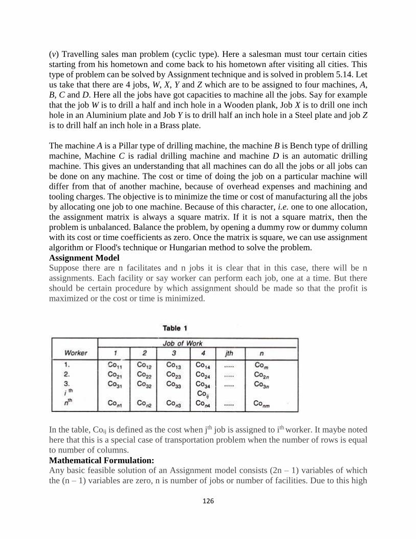
126

(v) Travelling sales man problem (cyclic type). Here a salesman must tour certain cities

starting from his hometown and come back to his hometown after visiting all cities. This

type of problem can be solved by Assignment technique and is solved in problem 5.14. Let

us take that there are 4 jobs, W, X, Y and Z which are to be assigned to four machines, A,

B, C and D. Here all the jobs have got capacities to machine all the jobs. Say for example

that the job W is to drill a half and inch hole in a Wooden plank, Job X is to drill one inch

hole in an Aluminium plate and Job Y is to drill half an inch hole in a Steel plate and job Z

is to drill half an inch hole in a Brass plate.

The machine A is a Pillar type of drilling machine, the machine B is Bench type of drilling

machine, Machine C is radial drilling machine and machine D is an automatic drilling

machine. This gives an understanding that all machines can do all the jobs or all jobs can

be done on any machine. The cost or time of doing the job on a particular machine will

differ from that of another machine, because of overhead expenses and machining and

tooling charges. The objective is to minimize the time or cost of manufacturing all the jobs

by allocating one job to one machine. Because of this character, i.e. one to one allocation,

the assignment matrix is always a square matrix. If it is not a square matrix, then the

problem is unbalanced. Balance the problem, by opening a dummy row or dummy column

with its cost or time coefficients as zero. Once the matrix is square, we can use assignment

algorithm or Flood's technique or Hungarian method to solve the problem.

Assignment Model

Suppose there are n facilitates and n jobs it is clear that in this case, there will be n

assignments. Each facility or say worker can perform each job, one at a time. But there

should be certain procedure by which assignment should be made so that the profit is

maximized or the cost or time is minimized.

In the table, Coij is defined as the cost when jth job is assigned to ith worker. It maybe noted

here that this is a special case of transportation problem when the number of rows is equal

to number of columns.

Mathematical Formulation:

Any basic feasible solution of an Assignment model consists (2n – 1) variables of which

the (n – 1) variables are zero, n is number of jobs or number of facilities. Due to this high

127

degeneracy, if we solve the problem by usual transportation method, it will be a complex

and time-consuming work. Thus, a separate technique is derived for it. Before going to the

absolute method, it is very important to formulate the problem.

Suppose xjj is a variable which is defined as

if the ith job is assigned to jth machine or facility

if the ith job is not assigned to jth machine or facility.

Now as the problem forms one to one basis or one job is to be assigned to one facility or

machine.

The total assignment cost will be given by

The above definition can be developed into mathematical model as follows:

Determine xij > 0 (i, j = 1,2, 3…n) in order to

Subjected to constraints

and xij is either zero or one.

Method to solve Problem (Hungarian Technique)

Consider the objective function of minimization type. Following steps are involved in

solving this Assignment problem,

https://cdn.yourarticlelibrary.com/wp-content/uploads/2014/04/clip_image004138.jpg

https://cdn.yourarticlelibrary.com/wp-content/uploads/2014/04/clip_image004138.jpg

128

1. Locate the smallest cost element in each row of the given cost table starting with the first

row. Now, this smallest element is subtracted from each element of that row. So, we will

be getting at least one zero in each row of this new table.

2. Having constructed the table (as by step-1) take the columns of the table. Starting from

first column locate the smallest cost element in each column. Now subtract this smallest

element from each element of that column. Having performed the step 1 and step 2, we

will be getting at least one zero in each column in the reduced cost table.

3. Now, the assignments are made for the reduced table in following manner.

(i) Rows are examined successively, until the row with exactly single (one) zero is found.

Assignment is made to this single zero by putting square □ around it and in the

corresponding column, all other zeros are crossed out (x) because these will not be used to

make any other assignment in this column. Step is conducted for each row.

(ii) Step 3 (i) in now performed on the columns as follow:- columns are examined

successively till a column with exactly one zero is found. Now, assignment is made to this

single zero by putting the square around it and at the same time, all other zeros in the

corresponding rows are crossed out (x) step is conducted for each column.

(iii) Step 3, (i) and 3 (ii) are repeated till all the zeros are either marked or crossed out.

Now, if the number of marked zeros or the assignments made are equal to number of rows

or columns, optimum solution has been achieved. There will be exactly single assignment

in each or columns without any assignment. In this case, we will go to step 4.

4. At this stage, draw the minimum number of lines (horizontal and vertical) necessary to

cover all zeros in the matrix obtained in step 3, Following procedure is adopted:

129

(i) Tick mark ( ) all rows that do not have any assignment.

(ii) Now tick mark( ) all these columns that have zero in the tick marked rows.

(iii) Now tick mark all the rows that are not already marked and that have assignment in

the marked columns.

(iv) All the steps i.e. (4(i), 4(ii), 4(iii) are repeated until no more rows or columns can be

marked.

(v) Now draw straight lines which pass through all the un marked rows and marked

columns. It can also be noticed that in an n x n matrix, always less than ‘n’ lines will cover

all the zeros if there is no solution among them.

5. In step 4, if the number of lines drawn are equal to n or the number of rows, then it is

the optimum solution if not, then go to step 6.

6. Select the smallest element among all the uncovered elements. Now, this element is

subtracted from all the uncovered elements and added to the element which lies at the

intersection of two lines. This is the matrix for fresh assignments.

7. Repeat the procedure from step (3) until the number of assignments becomes equal to

the number of rows or number of columns.

3.2 COMPARISION BETWEEN ASSIGNMENT MODEL AND

TRANSPORTATION MODEL

Now let us see what are the similarities and differences between Assignment Model

Transportation Model

Similarities

1. Both are special types of linear programming problems.

2. Both have objective function, structural constraints, and non-negativity constraints. And

the relationship between variables and constraints are linear.

3. The coefficients of variables in the solution will be either 1 or zero in both cases.

4. Both are basically minimization problems. For converting them into maximization

problem same procedure is used.

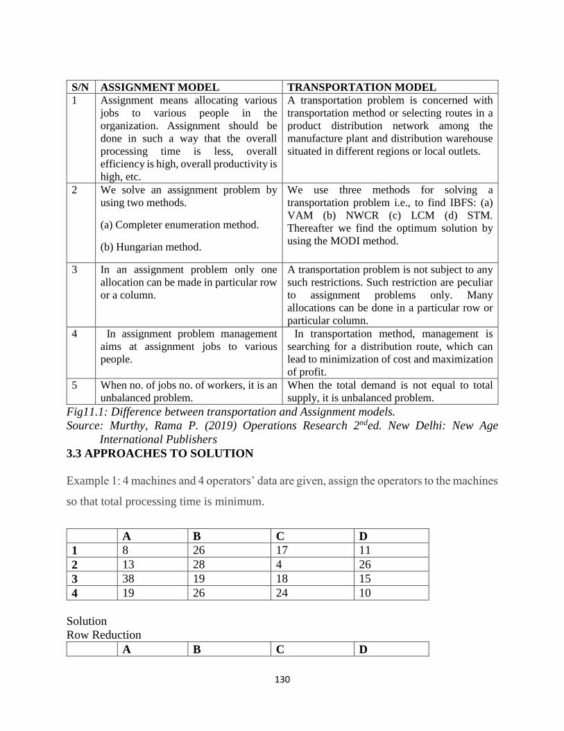
https://cdn.yourarticlelibrary.com/wp-content/uploads/2014/04/clip_image010.gif

https://cdn.yourarticlelibrary.com/wp-content/uploads/2014/04/clip_image0101.gif

130

S/N ASSIGNMENT MODEL TRANSPORTATION MODEL

1 Assignment means allocating various

jobs to various people in the

organization. Assignment should be

done in such a way that the overall

processing time is less, overall

efficiency is high, overall productivity is

high, etc.

A transportation problem is concerned with

transportation method or selecting routes in a

product distribution network among the

manufacture plant and distribution warehouse

situated in different regions or local outlets.

2 We solve an assignment problem by

using two methods.

(a) Completer enumeration method.

(b) Hungarian method.

We use three methods for solving a

transportation problem i.e., to find IBFS: (a)

VAM (b) NWCR (c) LCM (d) STM.

Thereafter we find the optimum solution by

using the MODI method.

3 In an assignment problem only one

allocation can be made in particular row

or a column.

A transportation problem is not subject to any

such restrictions. Such restriction are peculiar

to assignment problems only. Many

allocations can be done in a particular row or

particular column.

4 In assignment problem management

aims at assignment jobs to various

people.

In transportation method, management is

searching for a distribution route, which can

lead to minimization of cost and maximization

of profit.

5 When no. of jobs no. of workers, it is an

unbalanced problem.

When the total demand is not equal to total

supply, it is unbalanced problem.

Fig11.1: Difference between transportation and Assignment models.

Source: Murthy, Rama P. (2019) Operations Research 2nded. New Delhi: New Age

International Publishers

3.3 APPROACHES TO SOLUTION

Example 1: 4 machines and 4 operators’ data are given, assign the operators to the machines

so that total processing time is minimum.

A B C D

1 8 26 17 11

2 13 28 4 26

3 38 19 18 15

4 19 26 24 10

Solution

Row Reduction

A B C D

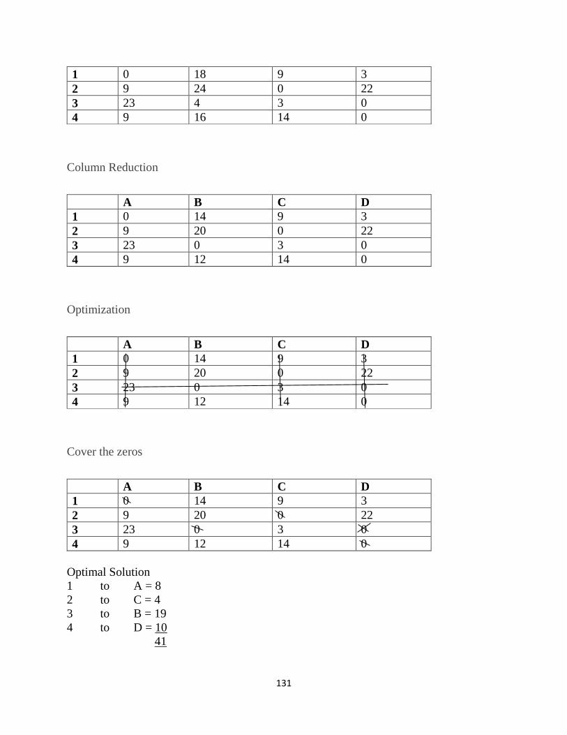
131

1 0 18 9 3

2 9 24 0 22

3 23 4 3 0

4 9 16 14 0

Column Reduction

A B C D

1 0 14 9 3

2 9 20 0 22

3 23 0 3 0

4 9 12 14 0

Optimization

A B C D

1 0 14 9 3

2 9 20 0 22

3 23 0 3 0

4 9 12 14 0

Cover the zeros

A B C D

1 0 14 9 3

2 9 20 0 22

3 23 0 3 0

4 9 12 14 0

Optimal Solution

1 to A = 8

2 to C = 4

3 to B = 19

4 to D = 10

41

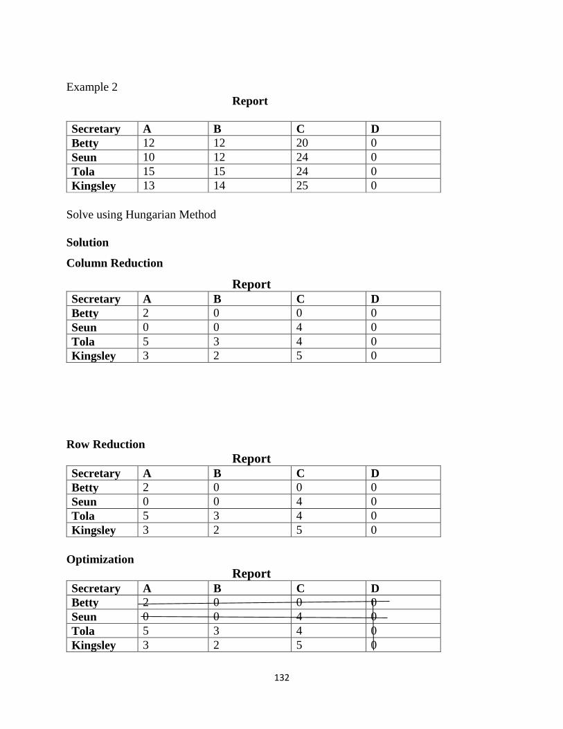
132

Example 2

Report

Secretary A B C D

Betty 12 12 20 0

Seun 10 12 24 0

Tola 15 15 24 0

Kingsley 13 14 25 0

Solve using Hungarian Method

Solution

Column Reduction

Report

Secretary A B C D

Betty 2 0 0 0

Seun 0 0 4 0

Tola 5 3 4 0

Kingsley 3 2 5 0

Row Reduction

Report

Secretary A B C D

Betty 2 0 0 0

Seun 0 0 4 0

Tola 5 3 4 0

Kingsley 3 2 5 0

Optimization

Report

Secretary A B C D

Betty 2 0 0 0

Seun 0 0 4 0

Tola 5 3 4 0

Kingsley 3 2 5 0

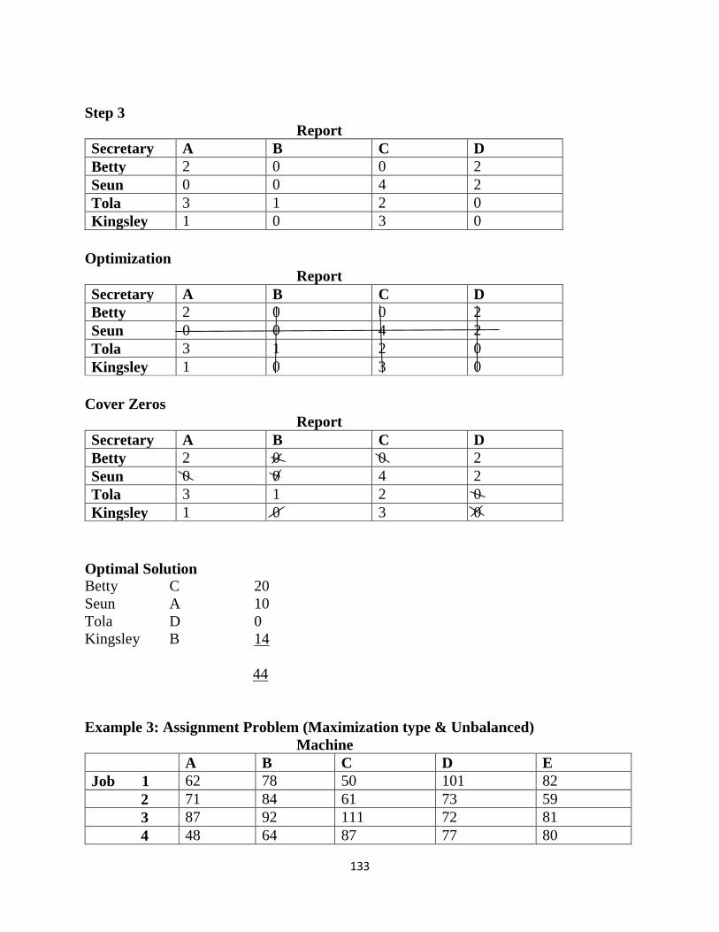
133

Step 3

Report

Secretary A B C D

Betty 2 0 0 2

Seun 0 0 4 2

Tola 3 1 2 0

Kingsley 1 0 3 0

Optimization

Report

Secretary A B C D

Betty 2 0 0 2

Seun 0 0 4 2

Tola 3 1 2 0

Kingsley 1 0 3 0

Cover Zeros

Report

Secretary A B C D

Betty 2 0 0 2

Seun 0 0 4 2

Tola 3 1 2 0

Kingsley 1 0 3 0

Optimal Solution

Betty C 20

Seun A 10

Tola D 0

Kingsley B 14

44

Example 3: Assignment Problem (Maximization type & Unbalanced)

Machine

A B C D E

Job 1 62 78 50 101 82

2 71 84 61 73 59

3 87 92 111 72 81

4 48 64 87 77 80

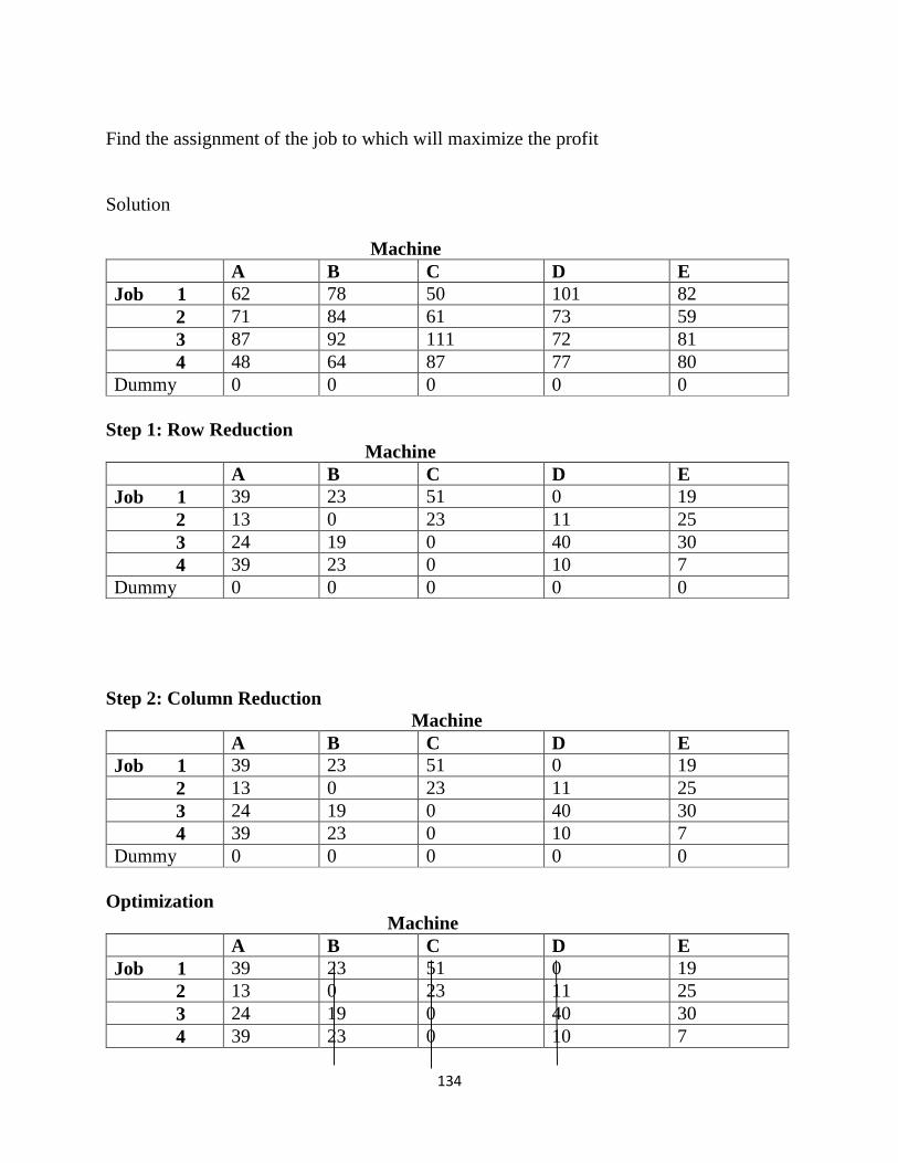
134

Find the assignment of the job to which will maximize the profit

Solution

Machine

A B C D E

Job 1 62 78 50 101 82

2 71 84 61 73 59

3 87 92 111 72 81

4 48 64 87 77 80

Dummy 0 0 0 0 0

Step 1: Row Reduction

Machine

A B C D E

Job 1 39 23 51 0 19

2 13 0 23 11 25

3 24 19 0 40 30

4 39 23 0 10 7

Dummy 0 0 0 0 0

Step 2: Column Reduction

Machine

A B C D E

Job 1 39 23 51 0 19

2 13 0 23 11 25

3 24 19 0 40 30

4 39 23 0 10 7

Dummy 0 0 0 0 0

Optimization

Machine

A B C D E

Job 1 39 23 51 0 19

2 13 0 23 11 25

3 24 19 0 40 30

4 39 23 0 10 7

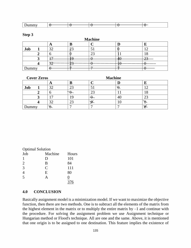
135

Dummy 0 0 0 0 0

Step 3

Machine

A B C D E

Job 1 32 23 51 0 12

2 6 0 23 11 18

3 17 19 0 40 23

4 32 23 0 10 0

Dummy 0 7 7 7 0

Cover Zeros Machine

A B C D E

Job 1 32 23 51 0 12

2 6 0 23 11 18

3 17 19 0 40 23

4 32 23 0 10 0

Dummy 0 7 7 7 0

Optimal Solution

Job Machine Hours

1 D 101

2 B 84

3 C 111

4 E 80

5 A 0

376

4.0 CONCLUSION

Basically assignment model is a minimization model. If we want to maximize the objective

function, then there are two methods. One is to subtract all the elements of the matrix from

the highest element in the matrix or to multiply the entire matrix by –1 and continue with

the procedure. For solving the assignment problem we use Assignment technique or

Hungarian method or Flood's technique. All are one and the same. Above, it is mentioned

that one origin is to be assigned to one destination. This feature implies the existence of

136

two specific characteristics in linear programming problems, which when present, give rise

to an assignment problem. The first one being the pay of matrix for a given problem is a

square matrix and the second is the optimum solution (or any solution with given

constraints) for the problem is such that there can be one and only one assignment in a

given row or column of the given payoff matrix.

5.0 SUMMARY

There various types of assignment problems these include: assigning the jobs to machines

when the problem has square matrix to minimize the time required to complete the jobs,

the second type is maximization type of assignment problem. Here we have to assign

certain jobs to certain facilities to maximize the returns or maximise the effectiveness,

Assignment problem having non-square matrix, Assignment problem with restrictions,

Travelling sales man problem, etc. there exist some similarities between assignment

problems and transportation problems. Some of the similarities include the fact that both

are special types of linear programming problems, both have objective function, structural

constraints, and non-negativity constraints.


List and explain five types of assignment problems.

Give three similarities between an assignment problem and a transportation

problem.

Highlight the differences between an assignment problem and a transportation

problem.

7.0 REFERENCES

Murthy, R.P. (2007). Operations Research 2nded. New Delhi: New Age International

Publishers.




Company.


Publications.


Nigeria.

137

UNIT 12: GAMES THEORY

1.0 Introduction

2.0 Objection

3.0 Main Content

3.1 Decision making

3.2 Description of a Game

3.3 Some Important Definitions in Games Theory

3.4 Assumptions Made in Games Theory

3.5 Description and Types of Games

3.5.1 Two-Person Zero-Sum Game

3.5.2 Pure Strategies

3.5.3 Dominating Strategies

3.5.4 Mixed Strategies

3.5.5 Optimal Strategies in 2 X 2 Matrix Game

3.5.6 Equilibrium Pairs

3.5.7 Optimal Strategies in 2 X N Matrix Game

138

3.5.8 Optimal Strategies for M X 2 Zero - Sum Games

4.0 Conclusion

5.0 Summary


7.0 References

1.0 INTRODUCTION

Game theory is the science of strategy. It attempts to determine mathematically and

logically the actions that “players” should take to secure the best outcomes for themselves

in a wide array of “games.” The games it studies range from chess to child rearing and

from tennis to takeovers. But the games all share the common feature of interdependence.

That is, the outcome for each participant depends on the choices (strategies) of all. In so-

called zero-sum games the interests of the players conflict totally, so that one person’s gain

always is another’s loss. More typical are games with the potential for either mutual gain

(positive sum) or mutual harm (negative sum), as well as some conflict.

Game theory was pioneered by Princeton mathematician JOHN VON NEUMANN. In the early

years the emphasis was on games of pure conflict (zero-sum games). Other games were

considered in a cooperative form. That is, the participants were supposed to choose and

implement their actions jointly. Recent research has focused on games that are neither zero

sum nor purely cooperative. In these games the players choose their actions separately, but

their links to others involve elements of both COMPETITION and cooperation.

Games are fundamentally different from decisions made in a neutral environment. To

illustrate the point, think of the difference between the decisions of a lumberjack and those

of a general. When the lumberjack decides how to chop wood, he does not expect the wood

to fight back; his environment is neutral. But when the general tries to cut down the

enemy’s army, he must anticipate and overcome resistance to his plans. Like the general,

a game player must recognize his interaction with other intelligent and purposive people.

His own choice must allow both for conflict and for possibilities for cooperation.

The essence of a game is the interdependence of player strategies. There are two distinct

types of strategic interdependence: sequential and simultaneous. In the former the players

move in sequence, each aware of the others’ previous actions. In the latter the players act

at the same time, each ignorant of the others’ actions.

A general principle for a player in a sequential-move game is to look ahead and reason

back. Each player should figure out how the other players will respond to his current move,

how he will respond in turn, and so on. The player anticipates where his initial decisions

will ultimately lead and uses this INFORMATION to calculate his current best choice. When

thinking about how others will respond, he must put himself in their shoes and think as

they would; he should not impose his own reasoning on them.

https://www.econlib.org/library/Enc/bios/Neumann.html

https://www.econlib.org/library/Enc/Competition.html

https://www.econlib.org/library/Enc/Information.html

139

In principle, any sequential game that ends after a finite sequence of moves can be “solved”

completely. We determine each player’s best strategy by looking ahead to every possible

outcome. Simple games, such as tic-tac-toe, can be solved in this way and are therefore not

challenging. For many other games, such as chess, the calculations are too complex to

perform in practice even with computers. Therefore, the players look a few moves ahead

and try to evaluate the resulting positions on the basis of experience.

In contrast to the linear chain of reasoning for sequential games, a game with simultaneous

moves involves a logical circle. Although the players act at the same time, in ignorance of

the others’ current actions, each must be aware that there are other players who are similarly

aware, and so on. The thinking goes: “I think that he thinks that I think”. Therefore, each

must figuratively put himself in the shoes of all and try to calculate the outcome. His own

best action is an integral part of this overall calculation.

This logical circle is squared (the circular reasoning is brought to a conclusion) using a

concept of equilibrium developed by the Princeton mathematician JOHN NASH. We look

for a set of choices, one for each player, such that each person’s strategy is best for him

when all others are playing their stipulated best strategies. In other words, each picks his

best response to what the others do.

Sometimes one person’s best choice is the same no matter what the others do. This is called

a “dominant strategy” for that player. At other times, one player has a uniformly bad choice

a “dominated strategy” in the sense that some other choice is better for him no matter what

the others do. The search for an equilibrium should begin by looking for dominant

strategies and eliminating dominated ones.

When we say that an outcome is an equilibrium, there is no presumption that each person’s

privately best choice will lead to a collectively optimal result. Indeed, there are notorious

examples, such as the PRISONERS’ DILEMMA, where the players are drawn into a bad

outcome by each following his best private interests.

Nash’s notion of equilibrium remains an incomplete solution to the problem of circular

reasoning in simultaneous-move games. Some games have many such equilibria while

others have none. And the dynamic process that can lead to an equilibrium is left

unspecified. But in spite of these flaws, the concept has proved extremely useful in

analyzing many strategic interactions.

It is often thought that the application of game theory requires all players to be

hyperrational. The theory makes no such claims. Players may be spiteful or envious as well

as charitable and empathetic. Recall George Bernard Shaw’s amendment to the Golden

Rule: “Do not do unto others as you would have them do unto you. Their tastes may be

different.” In addition to different motivations, other players may have different

https://www.econlib.org/library/Enc/bios/Nash.html

https://www.econlib.org/library/Enc/PrisonersDilemma.html

140

information. When calculating an equilibrium or anticipating the response to your move,

you always have to take the other players as they are, not as you are.

2.0 OBJECTIVES

By the end of this chapter, you will be able to:

Define the concept of a game

State the assumptions of games theory

Describe the two-person zero-sum games

Explain the concept of saddle point solution in a game

3.0 MAIN CONTENT

3.1 DECISION MAKING

Making decision is an integral and continuous aspect of human life. For child or adult,

man or woman, government official or business executive, worker or supervisor,

participation in the process of decision- making is a common feature of everyday life.

What does this process of decision making involve? What is a decision? How can we

analyze and systematize the solving of certain types of decision problems? Answers of all

such question are the subject matter of decision theory. Decision-making involves listing

the various alternatives and evaluating them economically and select best among them.

Two important stages in decision-making is: (i) making the decision and (ii)

Implementation of the decision.

3.2 DESCRIPTION OF A GAME

In our day-to-day life we see many games like Chess, Poker, Football, Base ball etc. All

the games are pleasure-giving games, which have the character of a competition and are

played according to well- structured rules and regulations and end in a victory of one or

the other team or group or a player. But we refer to the word game in this unit the

competition between two business organizations, which has more earning competitive

situations. In this chapter game is described as:

A competitive situation is called a game if it has the following characteristics (Assumption

made to define a game):

1. There is finite number of competitors called Players. This is to say that the game is

played by two or more number of business houses. The game may be for creating new

market, or to increase the market share or to increase the competitiveness of the product. 2. A play is played when each player chooses one of his courses of actions. The choices

are made simultaneously, so that no player knows his opponent's choice until he has

decided his own course of action. But in real world, a player makes the choices after the

opponent has announced his course of action.

Algebraic Sum of Gains and Losses: A game in which the gains of one player are the

141

losses of other player or the algebraic sum of gains of both players is equal to zero, the

game is known as Zero sum game (ZSG). In a zero sum game the algebraic sum of the

gains of all players after play is bound to be zero. i.e. If gi as the pay of to a player in an-

person game, then the game will be a zero sum game if sum of all gi is equal to zero.

In game theory, the resulting gains can easily be represented in the form of a matrix called

pay–off matrix or gain matrix as discussed in 3 above. A payoff matrix is a table, which

shows how payments should be made at end of a play or the game. Zero sum game is also

known as constant sum game. Conversely, if the sum of gains and losses does not equal

to zero, the game is a non zero-sum game. A game where two persons are playing the

game and the sum of gains and losses is equal to zero, the game is known as Two-Person

Zero-Sum Game (TPZSG). A good example of two- person game is the game of chess. A

good example of n- person game is the situation when several companies are engaged in

an intensive advertising campaign to capture a larger share of the market (Murthy, 2007)

3.3 SOME IMPORTANT DEFINITIONS IN GAMES THEORY

Adebayo et al (2010) provide the following important definitions in game theory.

Player: A player is an active participant in a game. The games can have two

persons(Two-person game) or more than two persons (Multi person or n-person

game)

Moves: A move could be a decision by player or the result of a chance event.

Game: A game is a sequence of moves that are defined by a set of rules that governs

the players’ moves. The sequence of moves may be simultaneous.

Decision maker: A decision-maker is a person or group of people in a committee

who makes the final choice among the alternatives. A decision-maker is then a

player in the game.

Objective: An objective is what a decision-maker aims at accomplishing by means

of his decision. The decision-maker may end up with more than one objective.

Behaviour: This could be any sequence of states in a system. The behaviours of a

system are overt while state trajectories are covert.

Decision: The forceful imposition of a constraint on a set of initially possible

alternatives.

Conflict: A condition in which two or more parties claim possession of something

they cannot all have simultaneously. It could also be described as a state in which

two or more decision-makers who have different objectives, act in the same system

or share the same resources. Examples are value conflicts, territorial conflict,

conflicts of interests etc.

Strategy: it is the predetermined rule by which a player decides his course of action

from a list of courses of action during the game. To decide a particular strategy, the

player needs to know the other’s strategy.

Perfect information. A game is said to have perfect information if at every move

in the game all players know the move that have already been made. This includes

any random outcomes.

142

Payoffs. This is the numerical return received by a player at the end of a game and

this return is associated with each combination of action taken by the player. We

talk of “expected payoff’ if its move has a random outcome.

• Zero-sum Game. A game is said to be zero sum if the sum of player’s payoff is

zero. The zero value is obtained by treating losses as negatives and adding up the

wins and the losses in the game. Common examples are baseball and poker games.

3.4 ASSUMPTIONS MADE IN GAMES THEORY

The following are assumptions made in games theory.

Each player (Decision-maker) has available to him two or more clearly specified

choices or sequence of choices (plays).

A game usually leads to a well-defined end-state that terminates the game. The end

state could be a win, a loss or a draw.

Simultaneous decisions by players are assumed in all games.

A specified payoff for each player is associated with an end state (eg sum of payoffs

for zero sum-games is zero in every end-state).

Repetition is assumed. A series of repetitive decisions or plays results in a game

Each decision-maker (player) has perfect knowledge of the game and of his

opposition i.e. he knows the rules of the game in details and also the payoffs of all

other players. The cost of collecting or knowing this information is not considered

in game theory.

All decision-makers are rational and will therefore always select among alternatives,

the alternative that gives him the greater payoff.

The last two assumptions are obviously not always practicable in real life situation. These

assumptions have revealed that game theory is a general theory of rational behaviour

involving two or more decision makers who have a limit number of courses of action of

plays, each leading to a well-defined outcome or ending with games and losses that can be

expressed as payoffs associated with each courses of action and for each decision maker.

The players have perfect knowledge of the opponent’s moves and are rational in taking

decision that optimises their individual gain.

The various conflicts can be represented by a matrix of payoffs. Game theory also proposes

several solutions to the game. Two of the proposed solutions are:

1. Minimax or pure Strategy: In a minimax strategy each player selects a strategy

that minimises the maximum loss his opponent can impose upon him.

2. Mixed Strategy: A mixed strategy which involves probability choices.

Lot of experiments have been performed on games with results showing conditions for (i)

Cooperation (ii) Defection and (iii) Persistence of conflict,

3.5 DESCRIPTION AND TYPES OF GAMES

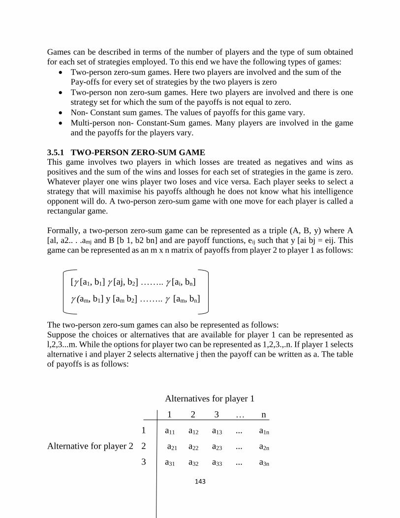
143

Games can be described in terms of the number of players and the type of sum obtained

for each set of strategies employed. To this end we have the following types of games:

Two-person zero-sum games. Here two players are involved and the sum of the

Pay-offs for every set of strategies by the two players is zero

Two-person non zero-sum games. Here two players are involved and there is one

strategy set for which the sum of the payoffs is not equal to zero.

Non- Constant sum games. The values of payoffs for this game vary.

Multi-person non- Constant-Sum games. Many players are involved in the game

and the payoffs for the players vary.

3.5.1 TWO-PERSON ZERO-SUM GAME This game involves two players in which losses are treated as negatives and wins as

positives and the sum of the wins and losses for each set of strategies in the game is zero.

Whatever player one wins player two loses and vice versa. Each player seeks to select a

strategy that will maximise his payoffs although he does not know what his intelligence

opponent will do. A two-person zero-sum game with one move for each player is called a

rectangular game.

Formally, a two-person zero-sum game can be represented as a triple (A, B, y) where A

[al, a2.. . .amj and B [b 1, b2 bn] and are payoff functions, eij such that y [ai bj = eij. This

game can be represented as an m x n matrix of payoffs from player 2 to player 1 as follows:

[ [a1, b1] [aj, b2] …….. [ai, bn]

(am, b1] y [am b2] …….. [am, bn]

The two-person zero-sum games can also be represented as follows:

Suppose the choices or alternatives that are available for player 1 can be represented as

l,2,3...m. While the options for player two can be represented as 1,2,3.,.n. If player 1 selects

alternative i and player 2 selects alternative j then the payoff can be written as a. The table

of payoffs is as follows:

Alternatives for player 1

1 2 3 … n

1 a11 a12 a13 ... a1n

Alternative for player 2 2 a21 a22 a23 ... a2n

3 a31 a32 a33 ... a3n

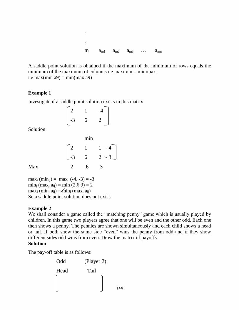
144

.

.

m am1 am2 am3 … amn

A saddle point solution is obtained if the maximum of the minimum of rows equals the

minimum of the maximum of columns i.e maximin = minimax

i.e max(min a9) = min(max a9)

Example 1

Investigate if a saddle point solution exists in this matrix

2 1 -4

-3 6 2

Solution

min

2 1 1 - 4

-3 6 2 - 3

Max 2 6 3

maxi (minij) = max (-4, -3) = -3

minj (maxj aij) = min (2,6,3) = 2

maxi (minj aij) = minj (maxi aij)

So a saddle point solution does not exist.

Example 2

We shall consider a game called the “matching penny” game which is usually played by

children. In this game two players agree that one will be even and the other odd. Each one

then shows a penny. The pennies are shown simultaneously and each child shows a head

or tail. If both show the same side “even” wins the penny from odd and if they show

different sides odd wins from even. Draw the matrix of payoffs

Solution

The pay-off table is as follows:

Odd (Player 2)

Head Tail

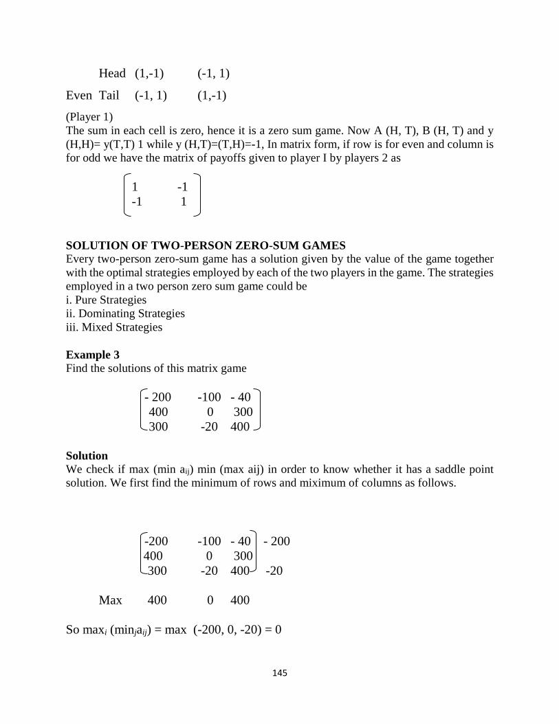
145

Head (1,-1) (-1, 1)

Even Tail (-1, 1) (1,-1)

(Player 1)

The sum in each cell is zero, hence it is a zero sum game. Now A (H, T), B (H, T) and y

(H,H)= y(T,T) 1 while y (H,T)=(T,H)=-1, In matrix form, if row is for even and column is

for odd we have the matrix of payoffs given to player I by players 2 as

1 -1

-1 1

SOLUTION OF TWO-PERSON ZERO-SUM GAMES

Every two-person zero-sum game has a solution given by the value of the game together

with the optimal strategies employed by each of the two players in the game. The strategies

employed in a two person zero sum game could be

i. Pure Strategies

ii. Dominating Strategies

iii. Mixed Strategies

Example 3

Find the solutions of this matrix game

- 200 -100 - 40

400 0 300

300 -20 400

Solution

We check if max (min aij) min (max aij) in order to know whether it has a saddle point

solution. We first find the minimum of rows and miximum of columns as follows.

-200 -100 - 40 - 200

400 0 300

300 -20 400 -20

Max 400 0 400

So maxi (minjaij) = max (-200, 0, -20) = 0

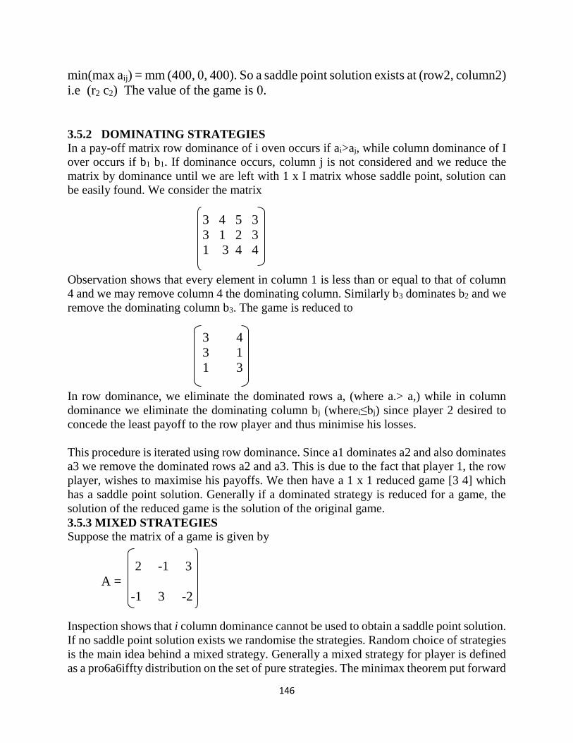
146

min(max aij) = mm (400, 0, 400). So a saddle point solution exists at (row2, column2)

i.e (r2 c2) The value of the game is 0.

3.5.2 DOMINATING STRATEGIES

In a pay-off matrix row dominance of i oven occurs if ai>aj, while column dominance of I

over occurs if b1 b1. If dominance occurs, column j is not considered and we reduce the

matrix by dominance until we are left with 1 x I matrix whose saddle point, solution can

be easily found. We consider the matrix

3 4 5 3

3 1 2 3

1 3 4 4

Observation shows that every element in column 1 is less than or equal to that of column

4 and we may remove column 4 the dominating column. Similarly b3 dominates b2 and we

remove the dominating column b3. The game is reduced to

3 4

3 1

1 3

In row dominance, we eliminate the dominated rows a, (where a.> a,) while in column

dominance we eliminate the dominating column bj (wherei≤bj) since player 2 desired to

concede the least payoff to the row player and thus minimise his losses.

This procedure is iterated using row dominance. Since a1 dominates a2 and also dominates

a3 we remove the dominated rows a2 and a3. This is due to the fact that player 1, the row

player, wishes to maximise his payoffs. We then have a 1 x 1 reduced game [3 4] which

has a saddle point solution. Generally if a dominated strategy is reduced for a game, the

solution of the reduced game is the solution of the original game.

3.5.3 MIXED STRATEGIES

Suppose the matrix of a game is given by

2 -1 3

A =

-1 3 -2

Inspection shows that i column dominance cannot be used to obtain a saddle point solution.

If no saddle point solution exists we randomise the strategies. Random choice of strategies

is the main idea behind a mixed strategy. Generally a mixed strategy for player is defined

as a pro6a6iffty distribution on the set of pure strategies. The minimax theorem put forward

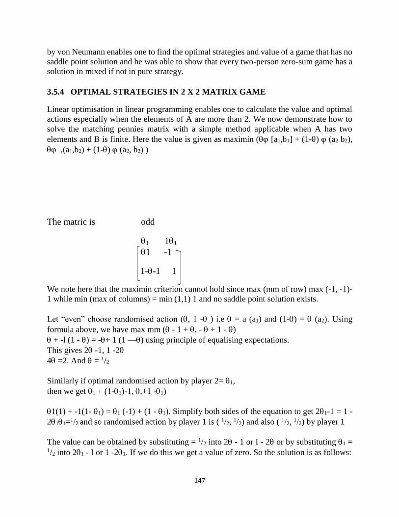
147

by von Neumann enables one to find the optimal strategies and value of a game that has no

saddle point solution and he was able to show that every two-person zero-sum game has a

solution in mixed if not in pure strategy.

3.5.4 OPTIMAL STRATEGIES IN 2 X 2 MATRIX GAME

Linear optimisation in linear programming enables one to calculate the value and optimal

actions especially when the elements of A are more than 2. We now demonstrate how to

solve the matching pennies matrix with a simple method applicable when A has two

elements and B is finite. Here the value is given as maximin ( [a1,b1] + (1-) (a2 b2),

,(a1,b2) + (1-) (a2, b2) )

The matric is odd

1 11

1 -1

1--1 1

We note here that the maximin criterion cannot hold since max (mm of row) max (-1, -1)-

1 while min (max of columns) = min (1,1) 1 and no saddle point solution exists.

Let “even” choose randomised action (, 1 - ) i.e = a (a1) and (1-) = (a2). Using

formula above, we have max mm ( - 1 + , - + 1 - )

+ -l (1 - ) = -+ 1 (1 —) using principle of equalising expectations.

This gives 2 -1, 1 -2

4 =2. And = 1/2

Similarly if optimal randomised action by player 2= 1,

then we get 1 + (1-1)-1, ,+1 -1)

1(1) + -1(1- 1) = 1 (-1) + (1 - 1). Simplify both sides of the equation to get 21-1 = 1 -

211=1/2 and so randomised action by player 1 is ( 1/2, 1/2) and also ( 1/2, 1/2) by player 1

The value can be obtained by substituting = 1/2 into 2 - 1 or I - 2 or by substituting 1 = 1/2 into 21 - I or 1 -21. If we do this we get a value of zero. So the solution is as follows:

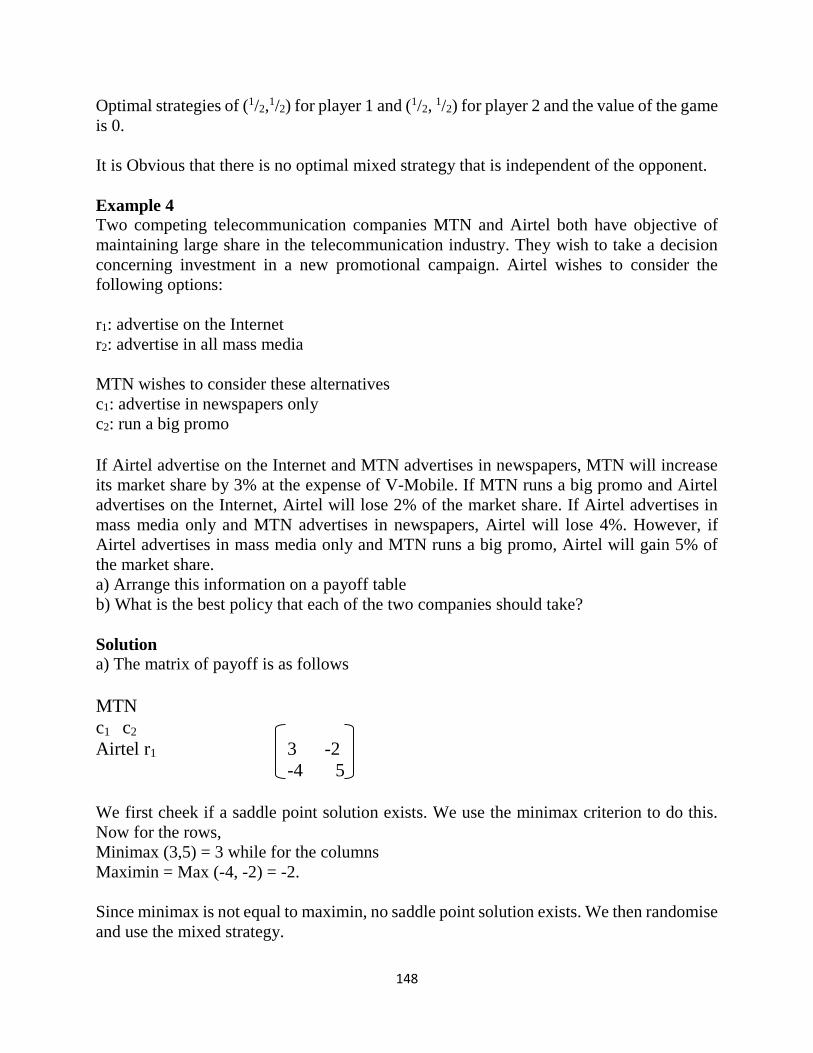
148

Optimal strategies of (1/2,1/2) for player 1 and (1/2, 1/2) for player 2 and the value of the game

is 0.

It is Obvious that there is no optimal mixed strategy that is independent of the opponent.

Example 4

Two competing telecommunication companies MTN and Airtel both have objective of

maintaining large share in the telecommunication industry. They wish to take a decision

concerning investment in a new promotional campaign. Airtel wishes to consider the

following options:

r1: advertise on the Internet

r2: advertise in all mass media

MTN wishes to consider these alternatives

c1: advertise in newspapers only

c2: run a big promo

If Airtel advertise on the Internet and MTN advertises in newspapers, MTN will increase

its market share by 3% at the expense of V-Mobile. If MTN runs a big promo and Airtel

advertises on the Internet, Airtel will lose 2% of the market share. If Airtel advertises in

mass media only and MTN advertises in newspapers, Airtel will lose 4%. However, if

Airtel advertises in mass media only and MTN runs a big promo, Airtel will gain 5% of

the market share.

a) Arrange this information on a payoff table

b) What is the best policy that each of the two companies should take?

Solution

a) The matrix of payoff is as follows

MTN

c1 c2

Airtel r1 3 -2

-4 5

We first cheek if a saddle point solution exists. We use the minimax criterion to do this.

Now for the rows,

Minimax (3,5) = 3 while for the columns

Maximin = Max (-4, -2) = -2.

Since minimax is not equal to maximin, no saddle point solution exists. We then randomise

and use the mixed strategy.

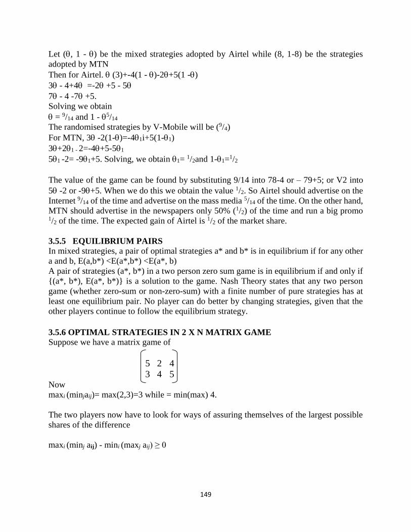
149

Let (, 1 - ) be the mixed strategies adopted by Airtel while (8, 1-8) be the strategies

adopted by MTN

Then for Airtel. (3)+-4(1 - )-2+5(1 -)

3 - 4+4 =-2 +5 - 5

7 - 4 -7 +5.

Solving we obtain

= 9/14 and 1 - 5/14

The randomised strategies by V-Mobile will be (9/4)

For MTN, 3 -2(1-)=-41i+5(1-1)

3+21 - 2=-4+5-51

51 -2= -91+5. Solving, we obtain 1= 1/2and 1-1=1/2

The value of the game can be found by substituting 9/14 into 78-4 or – 79+5; or V2 into

5 -2 or -9+5. When we do this we obtain the value 1/2. So Airtel should advertise on the

Internet 9/14 of the time and advertise on the mass media 5/14 of the time. On the other hand,

MTN should advertise in the newspapers only 50% (1/2) of the time and run a big promo 1/2 of the time. The expected gain of Airtel is 1/2 of the market share.

3.5.5 EQUILIBRIUM PAIRS

In mixed strategies, a pair of optimal strategies a* and b* is in equilibrium if for any other

a and b, E(a,b*) <E(a*,b*) <E(a*, b)

A pair of strategies (a*, b*) in a two person zero sum game is in equilibrium if and only if

{(a*, b*), E(a*, b*)} is a solution to the game. Nash Theory states that any two person

game (whether zero-sum or non-zero-sum) with a finite number of pure strategies has at

least one equilibrium pair. No player can do better by changing strategies, given that the

other players continue to follow the equilibrium strategy.

3.5.6 OPTIMAL STRATEGIES IN 2 X N MATRIX GAME

Suppose we have a matrix game of

5 2 4

3 4 5 Now

maxi (minjaij)= max(2,3)=3 while = min(max) 4.

The two players now have to look for ways of assuring themselves of the largest possible

shares of the difference

maxi (minj aij) - mini (maxj aij) ≥ 0

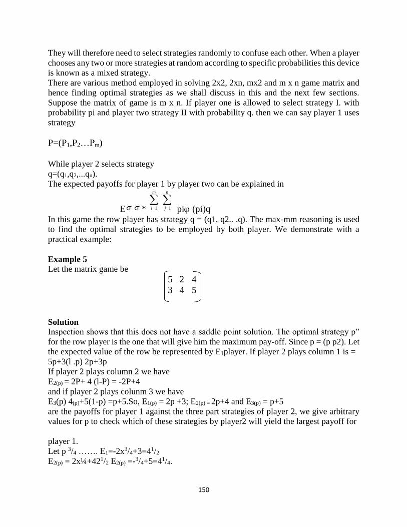
150

They will therefore need to select strategies randomly to confuse each other. When a player

chooses any two or more strategies at random according to specific probabilities this device

is known as a mixed strategy.

There are various method employed in solving 2x2, 2xn, mx2 and m x n game matrix and

hence finding optimal strategies as we shall discuss in this and the next few sections.

Suppose the matrix of game is m x n. If player one is allowed to select strategy I. with

probability pi and player two strategy II with probability q. then we can say player 1 uses

strategy

P=(P1,P2…Pm)

While player 2 selects strategy

q=(q1,q2,...qn).

The expected payoffs for player 1 by player two can be explained in

E *

n

j

m

i 11 pi (pi)q In this game the row player has strategy q = (q1, q2.. .q). The max-mm reasoning is used

to find the optimal strategies to be employed by both player. We demonstrate with a

practical example:

Example 5

Let the matrix game be

5 2 4

3 4 5

Solution

Inspection shows that this does not have a saddle point solution. The optimal strategy p”

for the row player is the one that will give him the maximum pay-off. Since p = (p p2). Let

the expected value of the row be represented by E1player. If player 2 plays column 1 is =

5p+3(l .p) 2p+3p

If player 2 plays column 2 we have

E2(p) = 2P+ 4 (l-P) = -2P+4

and if player 2 plays colunm 3 we have

E3(p) 4(p)+5(1-p) =p+5.So, E1(p) = 2p +3; E2(p) = 2p+4 and E3(p) = p+5

are the payoffs for player 1 against the three part strategies of player 2, we give arbitrary

values for p to check which of these strategies by player2 will yield the largest payoff for

player 1.

Let p 3/4 ……. E1=-2x3/4+3=41/2

E2(p) = 2x¼+421/2 E2(p) =-3/4+5=41/4.

151

So the two largest are E1(p), E3(p) and we equate them to get

2p = 3 = p+5

so 3p= 2, p=2/3

Ej(p) = (2 x 2/3) + 3 41/3

E = -2(p) -2 x 22/3 + 4 = 22/3 and E3(p) = 2/3 + 5 = 741/3

So(2/3, 1/3) is optimal for player 1. To get the optimal strategy for player 2, we observe that

it is advisable for player 2 to play column 2 in other to ensure that the payoff to row player

is minimal. So the game is reduced to

5 4

3 5

Let (q, l-q) be the strategy for player 2 in a required game.

So 5q + 4 (1-q) 3q +5(l-q)

5q+4-4q=3q+5-5q

q +45-2q

3q=l q=1/3

So it is optimal for player 2 to play mixed strategy with probability q(1/3,O,2/3).If we

substitute q = 1/3 into q+4 or 5-2q, we obtain 41/3 as before. This is the value of the game.

4.0 CONCLUSION

The theory of games (or game theory or competitive strategies) is a mathematical theory

that deals with the general features of competitive situations. This theory is helpful when

two or more individuals or organisations with conflicting objectives try to make decisions.

In such a situation, a decision made by on person affects the decision made by one or more

of the remaining decision makers, and the final outcome depend depends upon the decision

of all the parties.

5.0 SUMMARY

Making decision is an integral and continuous aspect of human life. For child or adult, man

or woman, government official or business executive, worker or supervisor, participation

in the process of decision- making is a common feature of everyday life. A competitive

situation is called a game if it has the following characteristics- there is finite number of

competitors called Players. A list of finite or infinite number of possible courses of action

is available to each player; a list of finite or infinite number of possible courses of action

is available to each player; a play is played when each player chooses one of his courses of

actions; all players act rationally and intelligently. Each player is interested in maximizing

his gains or minimizing his losses; each player makes individual decisions without direct

communication between the players; it is assumed that each player knows complete

relevant information.

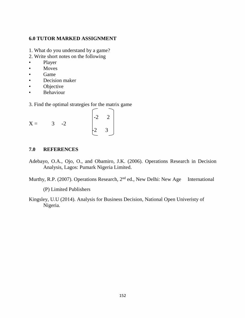
152


1. What do you understand by a game?

2. Write short notes on the following

• Player

• Moves

• Game

• Decision maker

• Objective

• Behaviour

3. Find the optimal strategies for the matrix game

-2 2

X = 3 -2

-2 3

7.0 REFERENCES

Adebayo, O.A., Ojo, O., and Obamiro, J.K. (2006). Operations Research in Decision


Murthy, R.P. (2007). Operations Research, 2nd ed., New Delhi: New Age International

(P) Limited Publishers


Nigeria.

153

MODULE FOUR

UNIT 13: PROJECT MANAGEMENT

1.0 Introduction

2.0 Objectives

3.0 Main Content

3.1 What is Project Management?

3.2 International Standards and Guidelines

3.3 Project Management Processes

3.4 Project vs. Product Life Cycles

3.5 What is the Value of Project Management?

3.6 How Project Management Relates to Other Disciplines

3.7 The Project Management Profession

3.8 Project Planning

3.9 Programme Evaluation and Review Technique and Critical Path Method

(PERT and CPM)

4.0 Conclusion

5.0 Summary


7.0 References

1.0 INTRODUCTION

154

This unit is designed to introduce you to the basic concepts and definitions associated with

project management. You will learn about the triple constraints of scope, time and cost; the

nine functional knowledge areas associated with project management and the four major

phases of a project. You will also learn about the skills and tools used to integrate all of the

knowledge areas throughout a project’s lifecycle. You will also learn how to use the CPM

and PERT techniques in solving project related problems.

2.0 OBJECTIVES


Define project management

Identify the “body of knowledge areas” in project management.

List and explain the processes involved in project management.

Describe the project vs product cycle.

3.0 MAIN CONTENT

3.1 WHAT IS PROJECT MANAGEMENT?

Project Management has been called an accidental profession. In many organisations in the

past, project managers typically stumbled or fell into project management responsibilities.

The world has since changed and project management is now recognised globally as a

formal discipline, with international standards and guidelines and a growing knowledge

base of best practices. Project management is the application of skills and knowledge and

the use of tools and techniques applied to activities in a project to complete the project as

defined in the scope. Project management is not only the use of a scheduling tool such as

Microsoft Project, Scheduler Plus, etc. Many organisations still do not understand that the

ability to use a scheduling tool is not enough to successfully manage a project. The use of

a tool is only one part of the equation. Project management requires a high level of skill in

both the people and technical side of the discipline for successful projects to result.

3.2 INTERNATIONAL STANDARDS AND GUIDELINES

Project Management is a formal discipline with international standards and guidelines

developed by the Project Management Institute (PMI). A significant body of knowledge

has been accumulated specifically over the past 5 years relating to effective project

management practices, tools, techniques and processes across industries. PMI is recognised

as the international body providing guidance and direction for the discipline. PMI has

developed the “Project Management Body of Knowledge” or “PMBOK” the essential

knowledge areas and processes required to effectively manage projects. There are nine

“body” of knowledge areas within the standards and guidelines.

• Integration Management: Processes to ensure that the elements of the project are

effectively coordinated. Integration management involves making decisions throughout the

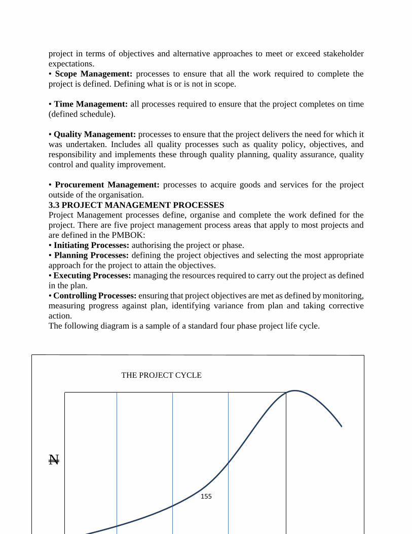
155

project in terms of objectives and alternative approaches to meet or exceed stakeholder

expectations.

• Scope Management: processes to ensure that all the work required to complete the

project is defined. Defining what is or is not in scope.

• Time Management: all processes required to ensure that the project completes on time

(defined schedule).

• Quality Management: processes to ensure that the project delivers the need for which it

was undertaken. Includes all quality processes such as quality policy, objectives, and

responsibility and implements these through quality planning, quality assurance, quality

control and quality improvement.

• Procurement Management: processes to acquire goods and services for the project

outside of the organisation.

3.3 PROJECT MANAGEMENT PROCESSES

Project Management processes define, organise and complete the work defined for the

project. There are five project management process areas that apply to most projects and

are defined in the PMBOK:

• Initiating Processes: authorising the project or phase.

• Planning Processes: defining the project objectives and selecting the most appropriate

approach for the project to attain the objectives.

• Executing Processes: managing the resources required to carry out the project as defined

in the plan.

• Controlling Processes: ensuring that project objectives are met as defined by monitoring,

measuring progress against plan, identifying variance from plan and taking corrective

action.

The following diagram is a sample of a standard four phase project life cycle.

THE PROJECT CYCLE

N

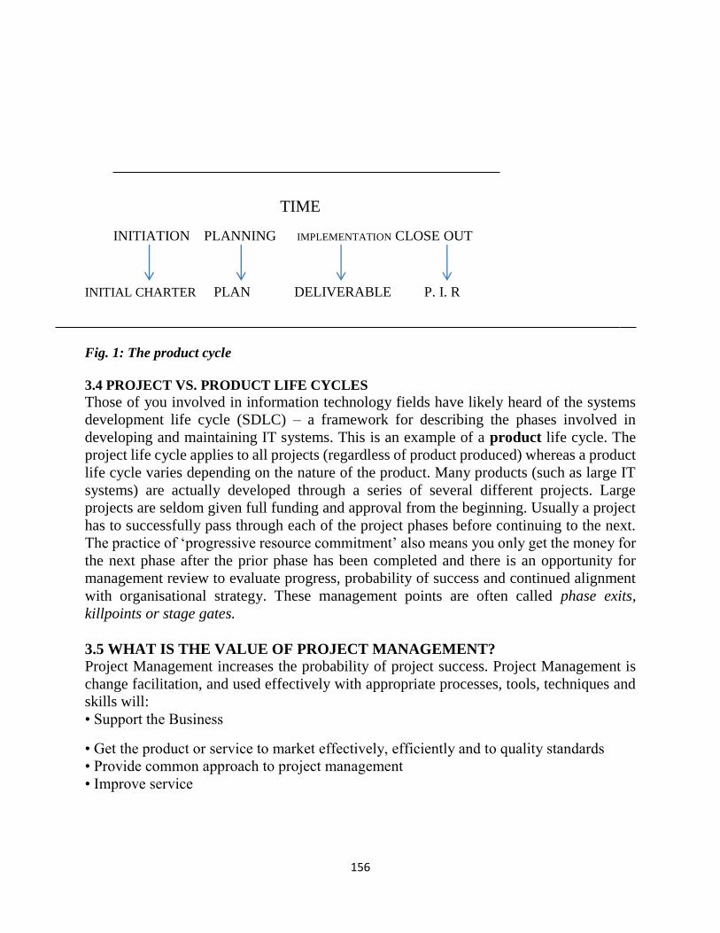
156

TIME

INITIATION PLANNING IMPLEMENTATION CLOSE OUT

INITIAL CHARTER PLAN DELIVERABLE P. I. R

Fig. 1: The product cycle

3.4 PROJECT VS. PRODUCT LIFE CYCLES

Those of you involved in information technology fields have likely heard of the systems

development life cycle (SDLC) – a framework for describing the phases involved in

developing and maintaining IT systems. This is an example of a product life cycle. The

project life cycle applies to all projects (regardless of product produced) whereas a product

life cycle varies depending on the nature of the product. Many products (such as large IT

systems) are actually developed through a series of several different projects. Large

projects are seldom given full funding and approval from the beginning. Usually a project

has to successfully pass through each of the project phases before continuing to the next.

The practice of ‘progressive resource commitment’ also means you only get the money for

the next phase after the prior phase has been completed and there is an opportunity for

management review to evaluate progress, probability of success and continued alignment

with organisational strategy. These management points are often called phase exits,

killpoints or stage gates.

3.5 WHAT IS THE VALUE OF PROJECT MANAGEMENT?

Project Management increases the probability of project success. Project Management is

change facilitation, and used effectively with appropriate processes, tools, techniques and

skills will:

• Support the Business

• Get the product or service to market effectively, efficiently and to quality standards

• Provide common approach to project management

• Improve service

157

Project management is the application of knowledge, skills, tools, and techniques to

project activities in order to meet or exceed stakeholder needs and expectations from a

project.

3.6 HOW PROJECT MANAGEMENT RELATES TO OTHER DISCIPLINES

Project management overlaps with general management knowledge and practice, as well

as with the project's application areas, knowledge, and practice. Project managers focus on

integrating all the pieces required for project completion. General Managers or operational

managers tend to focus on a particular discipline or functional area. In this respect, project

management tends to be a cross-functional role, often involving people from various

business areas and divisions. While project management requires some fundamental

understanding of the knowledge area of the project itself, the project manager does not

have to be an expert in that field.

3.7 THE PROJECT MANAGEMENT PROFESSION

The Project Management Institute (PMI) provides certification as a project management

professional (PMP). The requirements include verification of from 4500 to 7500 hours of

project management experience (depending on education level), adherence to a Code of

Ethics, and obtaining a score of 70% or higher on a 200-question multiple choice

certification exam. For further information see the PMI Internet website at

http://www.PMI.org.

3.8 PROJECT PLANNING We are going to take a quick look at the elements of project planning, starting with the

project life cycle and then examine the importance of detailed planning to the overall

success of the project. Without a clear definition of the project, it's impossible to discern

what should be delivered as a result. If requirements are not clear, your project will be

impossible to control, and it will become unmanageable. We will review the fundamentals

of planning and then move on to the importance of developing a comprehensive work

breakdown structure.

Today’s organisations are running at a fast pace. More so than ever, organisations are faced

with increasing global competition and as such, want products and services delivered

yesterday! Organisations are struggling with multiple projects, tight deadlines and fewer

skilled resources available to manage these projects. Project managers are struggling with

the concepts of best practices and the reality of life in a corporation.

Often, insufficient time is provided for planning the project appropriately and as a result

projects consistently fail to produce the expected results, have cost or time overruns, or just

plain fail. In such cases, the project manager can usually look back on his or her experiences

and see what went wrong, vowing never to make the same mistake again. Sometimes,

however, the cycle continues. Whether you manage a small, medium or large size project,

effective planning of the project is the single most critical step to success. Too many project

managers either neglect or spend too little time and effort planning. The tendency is to rush

to implementation before a clear picture is developed.

http://www.pmi.org/

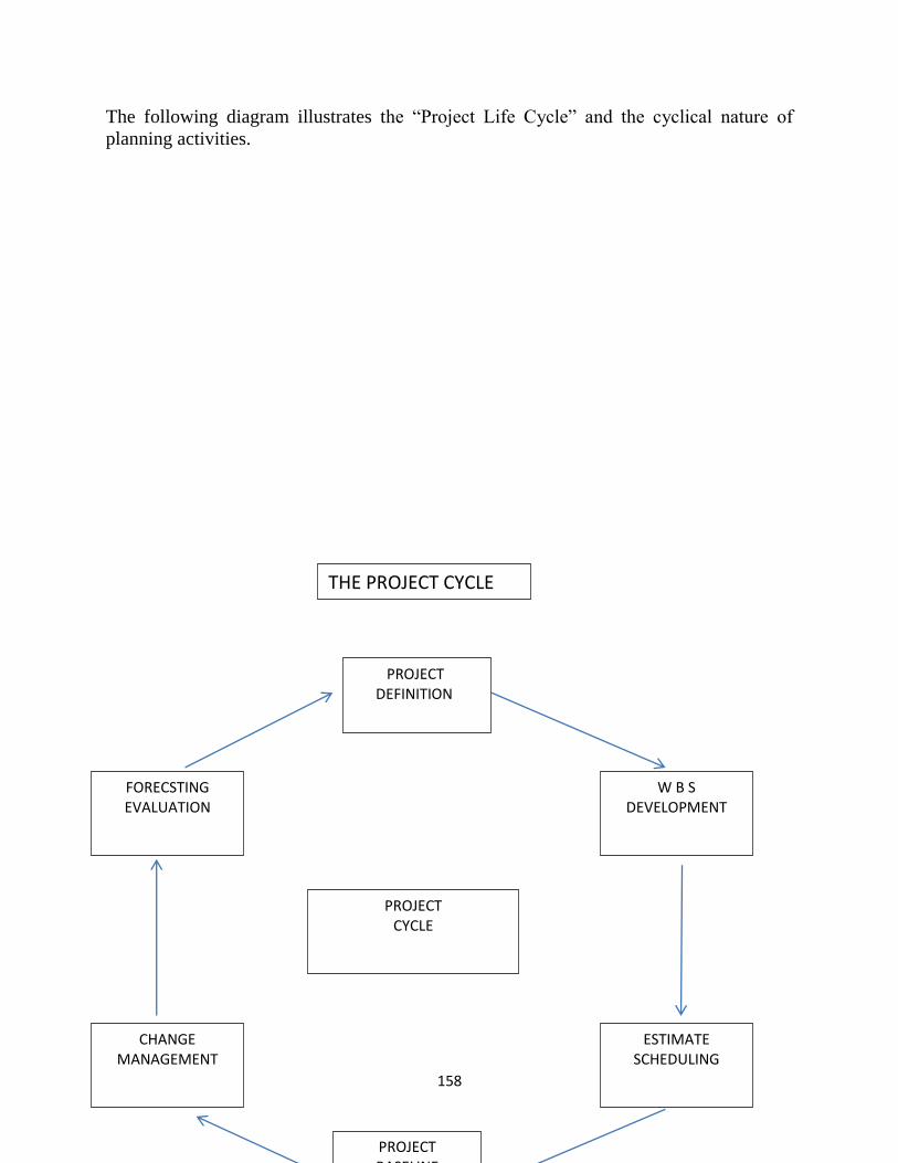
158

The following diagram illustrates the “Project Life Cycle” and the cyclical nature of

planning activities.

PROJECT CYCLE

PROJECT DEFINITION

PROJECT BASELINE

FORECSTING EVALUATION

CHANGE MANAGEMENT

ESTIMATE SCHEDULING

W B S DEVELOPMENT

THE PROJECT CYCLE

159

Fig. 2: The project cycle

3.9 PROGRAMME EVALUATION AND REVIEW TECHNIQUE AND

CRITICAL PATH METHOD (PERT AND CPM)

Programme Evaluation and Review Technique (PERT) and Critical Path Method (CPM)

are two techniques that are widely used in planning and scheduling the large projects. A

project is a combination of various activities. For example, Construction of a house can be

considered as a project. Similarly, conducting a public meeting may also be considered as

a project. In the above examples, construction of a house includes various activities such

as searching for a suitable site, arranging the finance, purchase of materials, digging the

foundation, construction of superstructure etc. Conducting a meeting includes, printing of

invitation cards, distribution of cards, arrangement of platform, chairs for audience etc. In

planning and scheduling the activities of large sized projects, the two network techniques

— PERT and CPM — are used conveniently to estimate and evaluate the project

completion time and control there sources to see that the project is completed within the

stipulated time and at minimum possible cost. Many managers, who use the PERT and

CPM techniques, have claimed that these techniques drastically reduce the project

completion time. But it is wrong to think that network analysis is a solution to all bad

management problems. In the present chapter, let us discuss how PERT and CPM are used

to schedule the projects. Initially, projects were represented by milestone chart and bar

chart. But they had little use in controlling the project activities. Bar chart simply

represents each activity by bars of length equal to the time taken on a common time scale

as shown in figure 15. l. This chart does not show interrelationship between activities. It is

very difficult to show the progress of work in these charts. An improvement in bar charts

is milestone chart. In milestone chart, key events of activities are identified and each

activity is connected to its preceding and succeeding activities to show the logical

relationship between activities. Here each key event is represented by a node (a circle) and

arrows instead of bars represent activities, as shown in figure the figures below. The

extension of milestone chart is PERT and CPM network methods.

Y

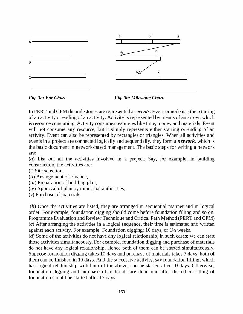
160

1 2 3 A

4 5

B

6 7 C

Fig. 3a: Bar Chart Fig. 3b: Milestone Chart.

In PERT and CPM the milestones are represented as events. Event or node is either starting

of an activity or ending of an activity. Activity is represented by means of an arrow, which

is resource consuming. Activity consumes resources like time, money and materials. Event

will not consume any resource, but it simply represents either starting or ending of an

activity. Event can also be represented by rectangles or triangles. When all activities and

events in a project are connected logically and sequentially, they form a network, which is

the basic document in network-based management. The basic steps for writing a network

are:

(a) List out all the activities involved in a project. Say, for example, in building

construction, the activities are:

(i) Site selection,

(ii) Arrangement of Finance,

(iii) Preparation of building plan,

(iv) Approval of plan by municipal authorities,

(v) Purchase of materials,

(b) Once the activities are listed, they are arranged in sequential manner and in logical

order. For example, foundation digging should come before foundation filling and so on.

Programme Evaluation and Review Technique and Critical Path Method (PERT and CPM)

(c) After arranging the activities in a logical sequence, their time is estimated and written

against each activity. For example: Foundation digging: 10 days, or 1½ weeks.

(d) Some of the activities do not have any logical relationship, in such cases; we can start

those activities simultaneously. For example, foundation digging and purchase of materials

do not have any logical relationship. Hence both of them can be started simultaneously.

Suppose foundation digging takes 10 days and purchase of materials takes 7 days, both of

them can be finished in 10 days. And the successive activity, say foundation filling, which

has logical relationship with both of the above, can be started after 10 days. Otherwise,

foundation digging and purchase of materials are done one after the other; filling of

foundation should be started after 17 days.

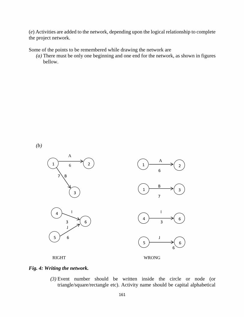
161

(e) Activities are added to the network, depending upon the logical relationship to complete

the project network.

Some of the points to be remembered while drawing the network are

(a) There must be only one beginning and one end for the network, as shown in figures

bellow.

(b)

A

A

6

6 7 B

B

7

I I

3 3 J

6 J

6

RIGHT WRONG

Fig. 4: Writing the network.

(3) Event number should be written inside the circle or node (or

triangle/square/rectangle etc). Activity name should be capital alphabetical

1 2

3

5

2

4

6

1

1 3

4 6

5 6

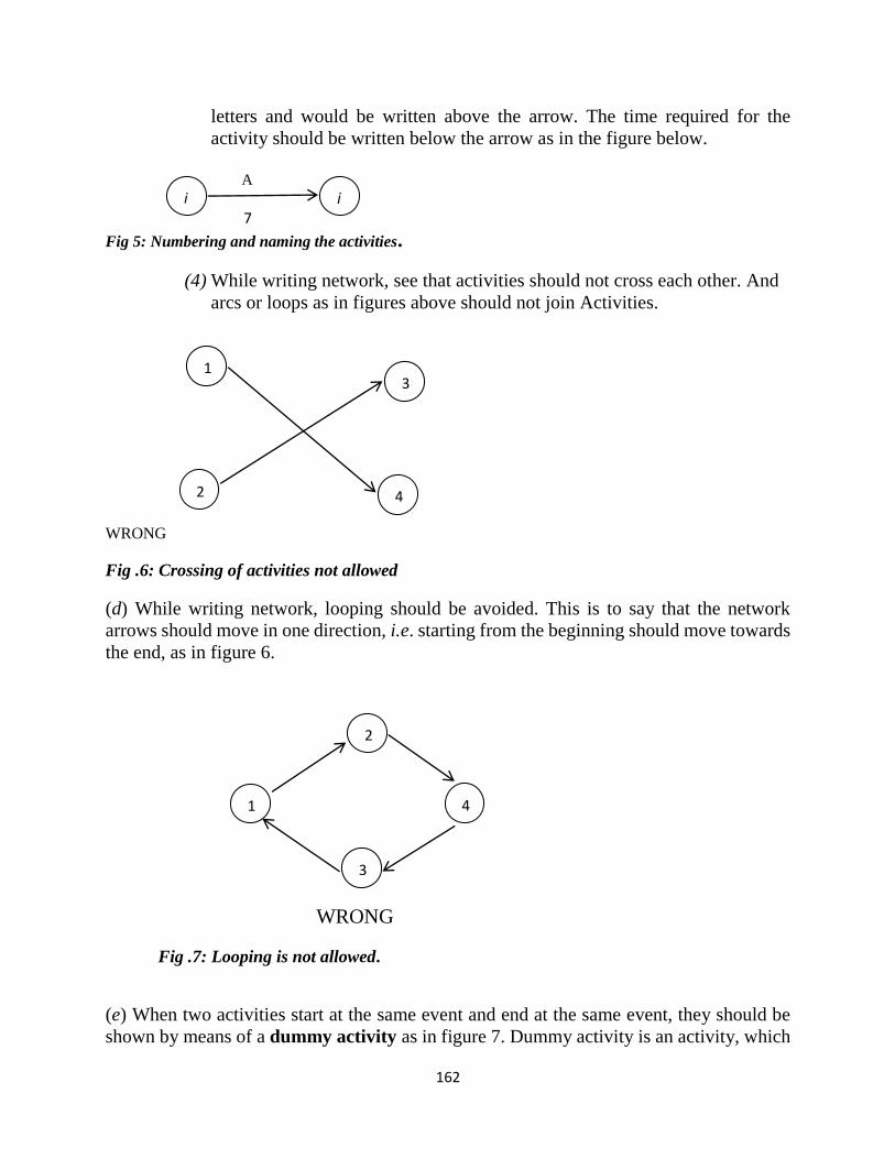
162

letters and would be written above the arrow. The time required for the

activity should be written below the arrow as in the figure below.

A

7

Fig 5: Numbering and naming the activities.

(4) While writing network, see that activities should not cross each other. And

arcs or loops as in figures above should not join Activities.

WRONG

Fig .6: Crossing of activities not allowed

(d) While writing network, looping should be avoided. This is to say that the network

arrows should move in one direction, i.e. starting from the beginning should move towards

the end, as in figure 6.

WRONG

Fig .7: Looping is not allowed.

(e) When two activities start at the same event and end at the same event, they should be

shown by means of a dummy activity as in figure 7. Dummy activity is an activity, which

i j

2

1

4

3

1

2

3

4

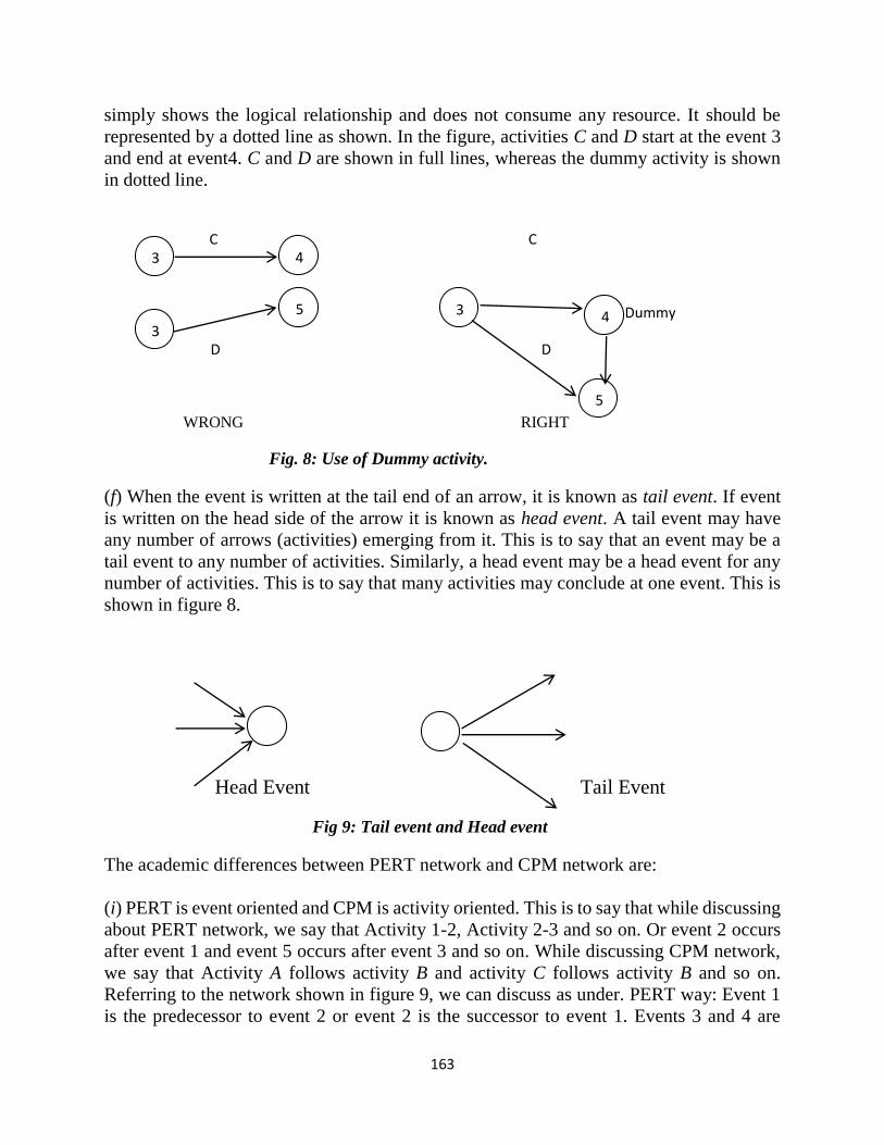
163

simply shows the logical relationship and does not consume any resource. It should be

represented by a dotted line as shown. In the figure, activities C and D start at the event 3

and end at event4. C and D are shown in full lines, whereas the dummy activity is shown

in dotted line. C C

Dummy

D D

WRONG RIGHT

Fig. 8: Use of Dummy activity.

(f) When the event is written at the tail end of an arrow, it is known as tail event. If event

is written on the head side of the arrow it is known as head event. A tail event may have

any number of arrows (activities) emerging from it. This is to say that an event may be a

tail event to any number of activities. Similarly, a head event may be a head event for any

number of activities. This is to say that many activities may conclude at one event. This is

shown in figure 8.

Head Event Tail Event

Fig 9: Tail event and Head event

The academic differences between PERT network and CPM network are:

(i) PERT is event oriented and CPM is activity oriented. This is to say that while discussing

about PERT network, we say that Activity 1-2, Activity 2-3 and so on. Or event 2 occurs

after event 1 and event 5 occurs after event 3 and so on. While discussing CPM network,

we say that Activity A follows activity B and activity C follows activity B and so on.

Referring to the network shown in figure 9, we can discuss as under. PERT way: Event 1

is the predecessor to event 2 or event 2 is the successor to event 1. Events 3 and 4 are

3 4

3 4 5 3

5

W

W

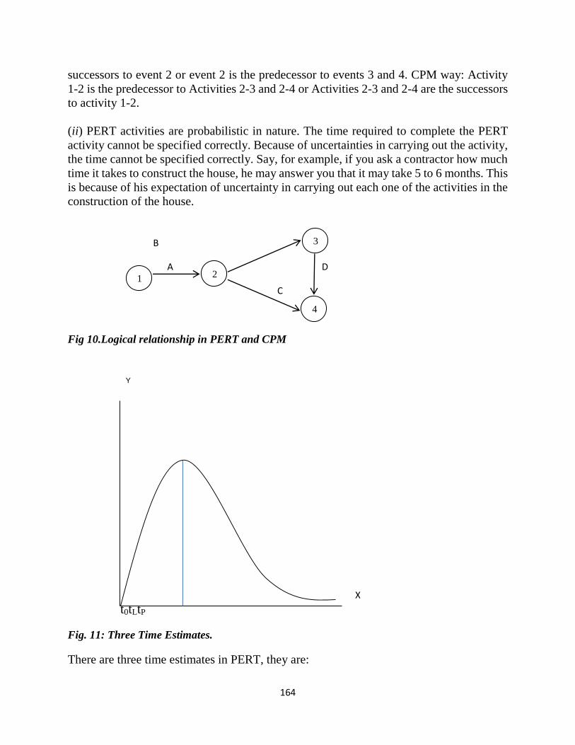
164

successors to event 2 or event 2 is the predecessor to events 3 and 4. CPM way: Activity

1-2 is the predecessor to Activities 2-3 and 2-4 or Activities 2-3 and 2-4 are the successors

to activity 1-2.

(ii) PERT activities are probabilistic in nature. The time required to complete the PERT

activity cannot be specified correctly. Because of uncertainties in carrying out the activity,

the time cannot be specified correctly. Say, for example, if you ask a contractor how much

time it takes to construct the house, he may answer you that it may take 5 to 6 months. This

is because of his expectation of uncertainty in carrying out each one of the activities in the

construction of the house.

B

A D

C

Fig 10.Logical relationship in PERT and CPM

Y

X

t0tLtP

Fig. 11: Three Time Estimates.

There are three time estimates in PERT, they are:

3

3

2

1

4

4

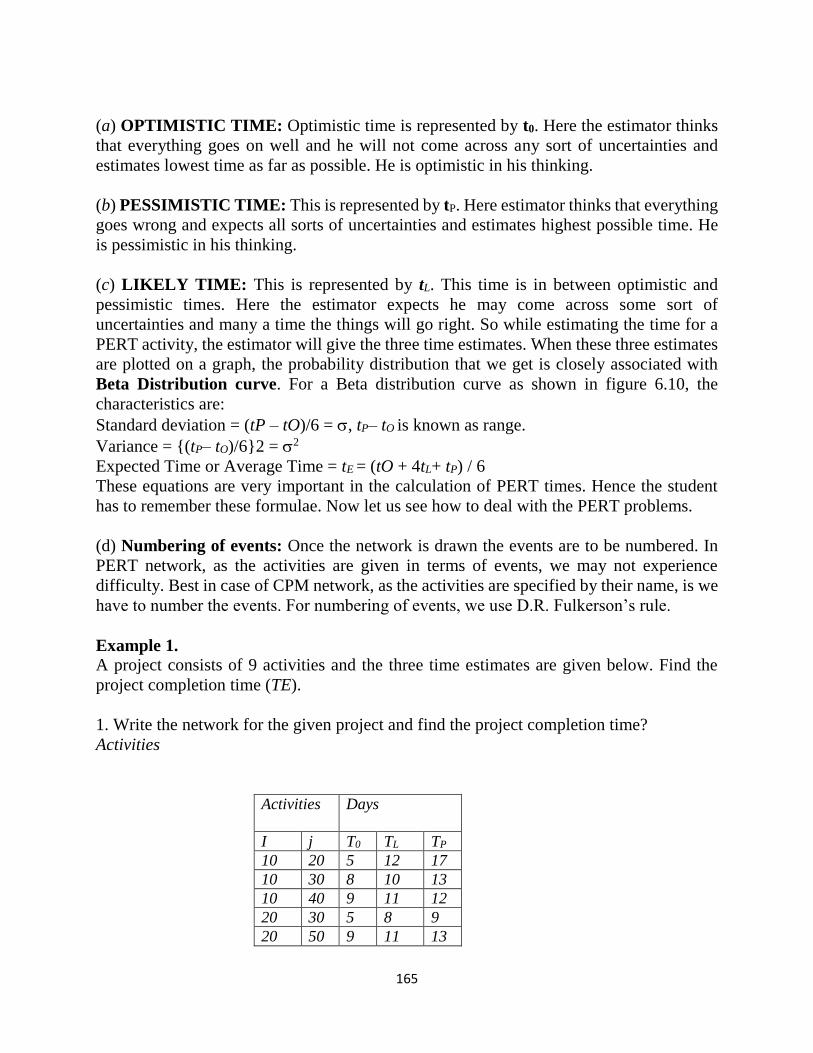
165

(a) OPTIMISTIC TIME: Optimistic time is represented by t0. Here the estimator thinks

that everything goes on well and he will not come across any sort of uncertainties and

estimates lowest time as far as possible. He is optimistic in his thinking.

(b) PESSIMISTIC TIME: This is represented by tP. Here estimator thinks that everything

goes wrong and expects all sorts of uncertainties and estimates highest possible time. He

is pessimistic in his thinking.

(c) LIKELY TIME: This is represented by tL. This time is in between optimistic and

pessimistic times. Here the estimator expects he may come across some sort of

uncertainties and many a time the things will go right. So while estimating the time for a

PERT activity, the estimator will give the three time estimates. When these three estimates

are plotted on a graph, the probability distribution that we get is closely associated with

Beta Distribution curve. For a Beta distribution curve as shown in figure 6.10, the

characteristics are:

Standard deviation = (tP – tO)/6 = , tP– tO is known as range.

Variance = {(tP– tO)/6}2 = 2

Expected Time or Average Time = tE = (tO + 4tL+ tP) / 6

These equations are very important in the calculation of PERT times. Hence the student

has to remember these formulae. Now let us see how to deal with the PERT problems.

(d) Numbering of events: Once the network is drawn the events are to be numbered. In

PERT network, as the activities are given in terms of events, we may not experience

difficulty. Best in case of CPM network, as the activities are specified by their name, is we

have to number the events. For numbering of events, we use D.R. Fulkerson’s rule.

Example 1.

A project consists of 9 activities and the three time estimates are given below. Find the

project completion time (TE).

1. Write the network for the given project and find the project completion time?

Activities

Activities Days

I j T0 TL TP

10 20 5 12 17

10 30 8 10 13

10 40 9 11 12

20 30 5 8 9

20 50 9 11 13

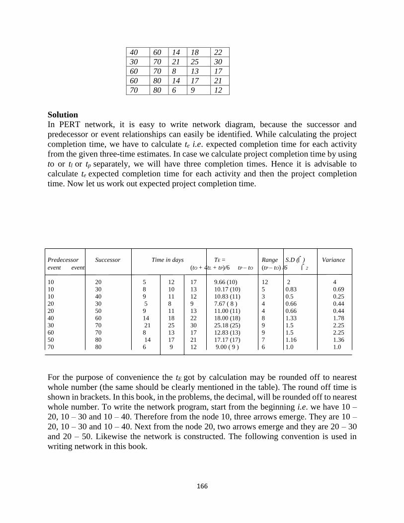
166

40 60 14 18 22

30 70 21 25 30

60 70 8 13 17

60 80 14 17 21

70 80 6 9 12

Solution

In PERT network, it is easy to write network diagram, because the successor and

predecessor or event relationships can easily be identified. While calculating the project

completion time, we have to calculate te i.e. expected completion time for each activity

from the given three-time estimates. In case we calculate project completion time by using

to or tl or tp separately, we will have three completion times. Hence it is advisable to

calculate te expected completion time for each activity and then the project completion

time. Now let us work out expected project completion time.

Predecessor Successor Time in days TE = Range S.D () Variance

event event (tO + 4tL + tP)/6 tP – tO (tP – tO) /6 2

10 20 5 12 17 9.66 (10) 12 2 4

10 30 8 10 13 10.17 (10) 5 0.83 0.69

10 40 9 11 12 10.83 (11) 3 0.5 0.25

20 30 5 8 9 7.67 ( 8 ) 4 0.66 0.44

20 50 9 11 13 11.00 (11) 4 0.66 0.44

40 60 14 18 22 18.00 (18) 8 1.33 1.78

30 70 21 25 30 25.18 (25) 9 1.5 2.25

60 70 8 13 17 12.83 (13) 9 1.5 2.25

50 80 14 17 21 17.17 (17) 7 1.16 1.36

70 80 6 9 12 9.00 ( 9 ) 6 1.0 1.0

For the purpose of convenience the tE got by calculation may be rounded off to nearest

whole number (the same should be clearly mentioned in the table). The round off time is

shown in brackets. In this book, in the problems, the decimal, will be rounded off to nearest

whole number. To write the network program, start from the beginning i.e. we have 10 –

20, 10 – 30 and 10 – 40. Therefore from the node 10, three arrows emerge. They are 10 –

20, 10 – 30 and 10 – 40. Next from the node 20, two arrows emerge and they are 20 – 30

and 20 – 50. Likewise the network is constructed. The following convention is used in

writing network in this book.

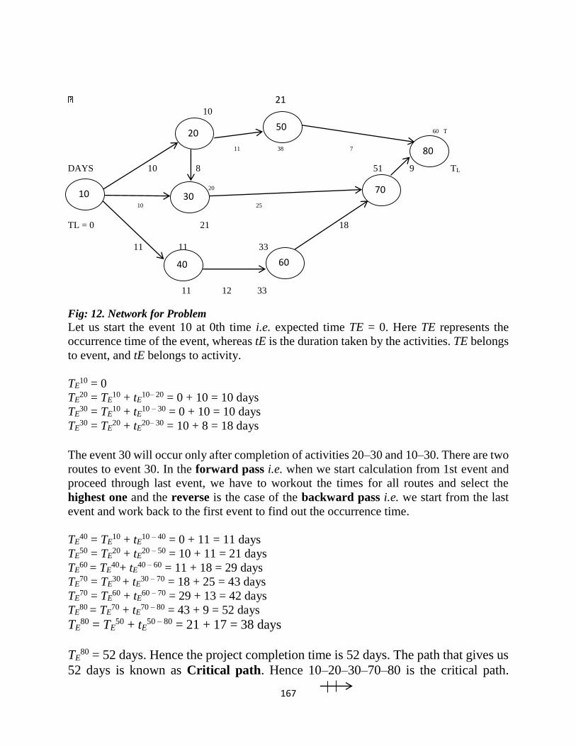
167

21 10

60 T

11 38 7

DAYS 10 8 51 9 TL

20

10 25

TL = 0 21 18

11 11 33

11 12 33

Fig: 12. Network for Problem

Let us start the event 10 at 0th time i.e. expected time TE = 0. Here TE represents the

occurrence time of the event, whereas tE is the duration taken by the activities. TE belongs

to event, and tE belongs to activity.

TE10 = 0

TE20 = TE

10 + tE10– 20 = 0 + 10 = 10 days

TE30 = TE

10 + tE10 – 30 = 0 + 10 = 10 days

TE30 = TE

20 + tE20– 30 = 10 + 8 = 18 days

The event 30 will occur only after completion of activities 20–30 and 10–30. There are two

routes to event 30. In the forward pass i.e. when we start calculation from 1st event and

proceed through last event, we have to workout the times for all routes and select the

highest one and the reverse is the case of the backward pass i.e. we start from the last

event and work back to the first event to find out the occurrence time.

TE40 = TE

10 + tE10 – 40 = 0 + 11 = 11 days

TE50 = TE

20 + tE20 – 50 = 10 + 11 = 21 days

TE60 = TE

40+ tE40 – 60 = 11 + 18 = 29 days

TE70 = TE

30 + tE30 – 70 = 18 + 25 = 43 days

TE70 = TE

60 + tE60 – 70 = 29 + 13 = 42 days

TE80 = TE

70 + tE70 – 80 = 43 + 9 = 52 days

TE80 = TE

50 + tE50 – 80 = 21 + 17 = 38 days

TE80 = 52 days. Hence the project completion time is 52 days. The path that gives us

52 days is known as Critical path. Hence 10–20–30–70–80 is the critical path.

10

50

80

70

60 40

30

20

168

Critical path is represented by a hatched line ( ). All other parts i.e. 10–40–60–

70–80, 10–20–50–80 and 10–30–70–80 are known as non-critical paths. All activities on

critical path are critical activities.

4.0 CONCLUSION

Project management is the application of skills and knowledge and the use of tools and

techniques applied to activities in a project to complete the project as defined in the scope.

Project management is not only the use of a scheduling tool such as Microsoft Project and

Scheduler Plus. Project management overlaps with general management knowledge and

practice, as well as with the project's application areas, knowledge, and practice.

Programme Evaluation and Review Technique (PERT) and Critical Path Method (CPM)

are two techniques that are widely used in planning and scheduling the large projects.

PERT is event oriented and CPM is activity oriented. PERT activities are probabilistic in

nature in the sense that the time required to complete the PERT activity cannot be specified

correctly.

5.0 SUMMARY

This unit treats the concept of project management. We defined Project management as the

application of skills and knowledge and the use of tools and techniques applied to activities

in a project to complete the project as defined in the scope. Project Management is a formal

discipline with international standards and guidelines developed by the Project

Management Institute (PMI). Project Management processes define, organise and

complete the work defined for the project. There are five project management process areas

that apply to most projects. They are: Initiating Processes, Planning Processes, Executing

Processes, Controlling Processes, and Closing Processes. Programme Evaluation and

Review Technique (PERT) and Critical Path Method (CPM) are two techniques that are

widely used in planning and scheduling the large projects. A project is a combination of

various activities.


Define project management.

Discuss the interrelationship between project management and other disciplines.

Identify and explain the five project management process areas that apply to most

projects.

Differentiate between PERT and CPM.

7.0 REFERENCES

Murthy, R.P. (2007). Operations Research 2nd ed. New Delhi: New Age International

Publishers.

169




Company.


Publications.


Nigeria.

UNIT 14: INVENTORY CONTROL

1.0 Introduction

2.0 Objective

3.0 Main Content

3.1 Definition of Inventory and Inventory Control

3.2 Basic Concepts in Inventory Planning

3.3 Necessity for Maintaining Inventory

3.4 Causes of Poor Inventory Control Systems

3.5 Classification of Inventories

3.6 Costs Associated With Inventory

3.7 Purpose of Maintaining Inventory or Objective of Inventory cost Control

3.8 Other Factors to be considered in Inventory Control

3.9 Inventory Control Problem

3.10 The Classical EOQ Model (Demand Rate Uniform, Replenishment Rate

Infinite)

4.0 Conclusion

5.0 Summary


7.0 References

1.0 INTRODUCTION

One of the basic functions of management is to employ capital efficiently so as to yield the

maximum returns. This can be done in either of two ways or by both, i.e. (a) By maximizing

the margin of profit; or (b) By maximizing the production with a given amount of capital,

170

i.e. to increase the productivity of capital. This means that the management should try to

make its capital work hard as possible. However, this is all too often neglected and much

time and ingenuity are devoted to make only labour work harder. In the process, the capital

turnover and hence the productivity of capital is often totally neglected.

Inventory management or Inventory Control is one of the techniques of Materials

Management which helps the management to improve the productivity of capital by

reducing the material costs, preventing the large amounts of capital being locked up for

long periods, and improving the capital - turnover ratio. The techniques of inventory

control were evolved and developed during and after the Second World War and have

helped the more industrially developed countries to make spectacular progress in

improving their productivity.

2.0 OBJECTIVES

At the this study unit, you should be able to

Define inventory control

Explain the basic concepts in inventory control

Identify the issues that necessitate maintaining inventory

Identify causes of poor inventory control systems

Discuss the various classifications of inventories

3.0 MAIN CONTENT

3.1 DEFINITION OF INVENTORY AND INVENTORY CONTROL

The word inventory means a physical stock of material or goods or commodities or other

economic resources that are stored or reserved or kept in stock or in hand for smooth and

efficient running of future affairs of an organization at the minimum cost of funds or capital

blocked in the form of materials or goods (Inventories). The function of directing the

movement of goods through the entire manufacturing cycle from the requisitioning of raw

materials to the inventory of finished goods in an orderly manner to meet the objectives of

maximum customer service with minimum investment and efficient (low cost) plant

operation is termed as inventory control. (Murthy, 2007)

Gupta and Hira (2012) defined an inventory as consisting of usable but idle resources such

as men, machines, materials, or money. When the resources involved are material, the

inventory is called stock. An inventory problem is said to exist if either the resources are

subject to control or if there is at least one such cost that decrease as inventory increases.

The objective is to minimise total (actual or expected) cost. However, in situations where

inventory affects demand, the objective may also be to minimise profit.

3.2 BASIC CONCEPTS IN INVENTORY PLANNING

For many organizations, inventories represent a major capital cost, in some cases the

dominant cost, so that the management of this capital becomes of the utmost importance.

171

When considering the inventories, we need to distinguish different classes of items that are

kept in stock. In practice, it turns out that about 10% of the items that are kept in stock

usually account for something in the order of 60% of the value of all inventories. Such

items are therefore of prime concern to the company, and the stock of these items will need

close attention. These most important items are usually referred to as “A items” in the ABC

classification system developed by the General Electric Company in the 1950s. The items

next in line are the B items, which are of intermediate importance. They typically represent

30% of the items, corresponding to about 30% of the total inventory value. Clearly, B items

do require some attention, but obviously less than A items. Finally, the bottom 60% of the

items are the C items. They usually represent maybe 10% of the monetary value of the total

inventory. The control of C items in inventory planning is less crucial than that of the A

and B items. The models in this chapter are mostly aimed at A items.

3.3 NECESSITY FOR MAINTAINING INVENTORY

Though inventory of materials is an idle resource (since materials lie idle and are not to be

used immediately), almost every organisation. Without it, no business activity can be

performed, whether it is service organisation like a hospital or a bank or it a manufacturing

or trading organisation. Gupta and Hira (2012) present the following reasons for maintain

inventories in organisations.

1. It helps in the smooth and efficient of an enterprise.

2. It helps in providing service to the customer at short notice.

3. In the absence of inventory, the enterprise may have to pay high prices due to

piecemeal purchasing.

4. It reduces product cost since there is an added advantage of batching and long,

uninterrupted production runs.

5. It acts as a buffer stock when raw materials are received late and shop rejection is

too many.

3.4 CAUSES OF POOR INVENTORY CONTROL SYSTEMS

a. Overbuying without regard to the forecast or proper estimate of demand to take

advantages of favourable market.

b. Overproduction or production of goods much before the customer requires them

c. Overstocking may also result from the desire to provide better service to the custom.

d. Cancellation of orders and minimum quantity stipulations by the suppliers may also

give rise to large inventories.


3.5 CLASSIFICATION OF INVENTORIES

Inventories may be classified as those which play direct role during manufacture or which

can be identified on the product and the second one are those which are required for

manufacturing but not as a part of production or cannot be identified on the product. The

first type is labelled as direct inventories and the second are labelled as indirect

inventories. Further classification of direct and indirect inventories is as follows:

A. Direct inventories

172

(i) Raw material inventories or Production Inventories: The inventory of raw materials

is the materials used in the manufacture of product and can be identified on the product. In

inventory control manager can concentrate on the

(a) Bulk purchase of materials to save the investment,

(b) To meet the changes in production rate,

(c) To plan for buffer stock or safety stock to serve against the delay in delivery of

inventory against orders placed and also against seasonal fluctuations. Direct inventories

include the following:

Production Inventories- items such as raw materials, components and

subassemblies used to produce the final products.

Work-in-progress Inventory- items in semi-finished form or products at different

stages of production.

Miscellaneous Inventory- all other items such as scrap, obsolete and unsaleable

products, stationary and other items used in office, factory and sales department,

etc.

(ii) Work-in -process inventories or in process inventories: These inventories are of semi-

finished type, which are accumulated between operations or facilities.As far as possible,

holding of materials between operations to be minimized if not avoided. This is because;

as we process the materials the economic value (added labour cost) and use value are added

to the raw material, which is drawn from stores. Hence if we hold these semi-finished

material for a

long time the inventory carrying cost goes on increasing, which is not advisable in

inventory control. These inventories serve the following purposes:

(a) Provide economical lot production,

(b) Cater to the variety of products,

(c) Replacement of wastages,

(d) To maintain uniform production even if sales varies.

(iii) Finished goods inventories: After finishing the production process and packing, the

finished products are stocked in stock room. These are known as finished goods inventory.

These are maintained to:

(a) To ensure the adequate supply to the customers,

(b) To allow stabilization of the production level and

(c) To help sales promotion programme.

(iv) MRO Inventory or Spare parts inventories: Maintenance, Repair, and Operation items

such as spare parts and consumable stores that do not go into final products but are

consumed during the production process. Any product sold to the customer, will be

subjected to wear and tear due to usage and the customer has to replace the worn-out part.

Hence the manufacturers always calculate the life of the various components of his product

and try to supply the spare components to the market to help after sales service. The use of

such spare parts inventory is:

(a) To provide after sales service to the customer,

173

(b) To utilize the product fully and economically by the customer.

(iv) Scrap or waste inventory or Miscellaneous Inventory: While processing the materials,

we may come across certain wastages and certain bad components (scrap), which are of no

use. These may be used by some other industries as raw material. These are to be collected

and kept in a place away from main stores and are disposed periodically by auctioning.

B. Indirect Inventories

Inventories or materials like oils, grease, lubricants, cotton waste and such other materials

are required during the production process. But we cannot identify them on the product.

These are known as indirect inventories. In our discussion of inventories, in this chapter,

we only discuss about the direct inventories. Inventories may also be classified depending

on their nature of use. They are:

(i) Fluctuation Inventories: These inventories are carried out to safeguard the fluctuation

in demand, non-delivery of material in time due to extended lead-time. These are

sometimes called as Safety stock or reserves. In real world inventory situations, the

material may not be received in time as expected due to trouble in transport system or some

times, the demand for a certain material may increase unexpectedly. To safeguard such

situations, safety stocks are maintained. The level of this stock will fluctuate depending on

the demand and lead-time etc.

(ii) Anticipation inventory: When there is an indication that the demand for company’s

product is going to be increased in the coming season, a large stock of material is stored in

anticipation. Some times in anticipation of raising prices, the material is stocked. Such

inventories, which are stocked in anticipation of raising demand or raising rises, are known

as anticipation inventories.

(iii) Lot size inventory or Cycle inventories: This situation happens in batch production

system. In this system products are produced in economic batch quantities. It sometime

happens that the materials are procured in quantities larger than the economic quantities to

meet the fluctuation in demand. In such cases the excess materials are stocked, which are

known as lot size or cycle inventories.

3.6 COSTS ASSOCIATED WITH INVENTORY

While maintaining the inventories, we will come across certain costs associated with

inventory, which are known as economic parameters. Most important of them are

discussed below:

A. Inventory Carrying Charges, or Inventory Carrying Cost or Holding Cost or

Storage Cost (C1) or (i%)

This cost arises due to holding of stock of material in stock. This cost includes the cost of

maintaining the inventory and is proportional to the quantity of material held in stock and

the time for which the material is maintained in stock. The components of inventory

carrying cost are:

174

i. Rent for the building in which the stock is maintained if it is a rented building. In case it

is own building, depreciation cost of the building is taken into consideration. Sometimes

for own buildings, the nominal rent is calculated depending on the local rate of rent and is

taken into consideration.

ii. It includes the cost of equipment if any and cost of racks and any special facilities used

in the stores.

iii. Interest on the money locked in the form of inventory or on the money invested in

purchasing the inventory.

iv. The cost of stationery used for maintaining the inventory.

v. The wages of personnel working in the stores.

vi. Cost of depreciation, insurance.

B. Shortage cost or Stock - out - cost- (C2)

Sometimes it so happens that the material may not be available when needed or when the

demand arises. In such cases the production has to be stopped until the procurement of the

material, which may lead to miss the delivery dates or delayed production. When the

organization could not meet the delivery promises, it has to pay penalty to the customer. If

the situation of stock out will occur very often, then the customer may not come to the

organization to place orders that is the organization is losing the customers In other words,

the organization is losing the goodwill of the customers The cost of good will cannot be

estimated. In some cases it will be very heavy to such extent that the organization has to

forego its business. Here to avoid the stock out situation, if the organization stocks more

material, inventory carrying cost increases and to take care of inventory cost, if the

organization purchases just sufficient or less quantity, then the stock out position may arise.

Hence the inventory manager must have sound knowledge of various factors that are

related to inventory carrying cost andstock out cost and estimate the quantity of material

to be purchased or else he must have effective strategies to face grave situations. The cost

is generally represented as so many naira and is represented by C2.

C. Set up cost or Ordering cost or Replenishment Cost (C3)

For purchase models, the cost is termed as ordering cost or procurement cost and for

manufacturing cost it is termed as set up cost and is represented by C3.

(i) Set up cost: The term set up cost is used for production or manufacturing models.

Whenever a job is to be produced, the machine is to set to produce the job. That is the tool

is to be set and the material is to be fixed in the jobholder. This consumes some time.

During this time the machine will be idle and the labour is working. The cost of idle

machine and cost of labour charges are to be added to the cost of production. If we produce

only one job in one set up, the entire set up cost is to be charged to one job only. In case

175

we produce ‘n’ number of jobs in one set up, the set up cost is shared by ‘n’ jobs. In case

of certain machines like N.C machines, or Jig boarding machine, the set up time may be

15 to 20 hours. The idle cost of the machine and labour charges may work out to few

thousands of naira. Once the machine set up is over, the entire production can be completed

in few hours if we produce more number of products in one set up the set up cost is allocated

to all the jobs equally. This

reduces the production cost of the product. For example let us assume that the set up cost

is N 1000/-. If we produce 10 jobs in one set up, each job is charged with N 100/- towards

the set up cost. In case, if we produce 100 jobs, the set up cost per job will be N10/-. If we

produce, 1000 jobs in one set up, the set up cost per job will be Re. 1/- only. This can be

shown by means of a graph as shown in figure 15.1.

(ii) Ordering Cost or Replenishment Cost: The term Ordering cost or Replenishment cost

is used in purchase models. Whenever any material is to be procured by an organization, it

has to place an order with the supplier. The cost of stationary used for placing the order,

the cost of salary of officials involved in preparing the order and the postal expenses and

after placing the order enquiry charges all put together, is known as ordering cost. In Small

Scale Units, this may be around N 25/- to N 30/- per order. In Larger Scale Industries, it

will be around N 150 to N 200 /- per order. In Government organizations, it may work out

to N 500/- and above per order. If the organization purchases more items per order, all the

items share the ordering cost. Hence the materials manager must decide how much to

purchase per order so as to keep the ordering cost per item at minimum. One point we have

to remember here, to reduce the ordering cost per item, if we purchase more items, the

inventory carrying cost increases. To keep inventory carrying cost under control, if we

purchase less quantity, the ordering cost increase. Hence one must be careful enough to

decide how much to purchase? The nature of ordering cost can also be shown by a graph

as shown in figure 8.1. If the ordering cost is C3 per order (can be equally applied to set up

cost) and the quantity ordered / produced is ‘q’ then the ordering cost or set up cost per unit

will be C3/q is inversely proportional to the quantity ordered, i.e. decreased with the

increase

in ‘q’ as shown in the graph below.

C0

(q/2)C1

Ordering cost

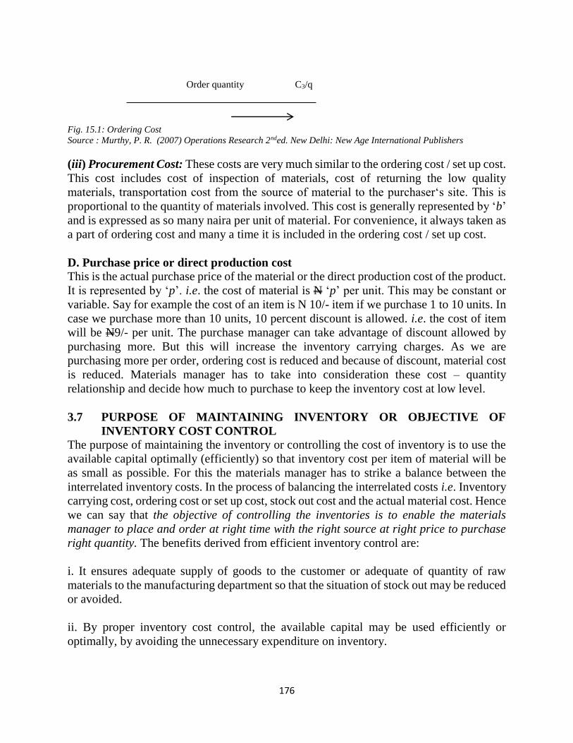
176

Order quantity C3/q

Fig. 15.1: Ordering Cost

Source : Murthy, P. R. (2007) Operations Research 2nded. New Delhi: New Age International Publishers

(iii) Procurement Cost: These costs are very much similar to the ordering cost / set up cost.

This cost includes cost of inspection of materials, cost of returning the low quality

materials, transportation cost from the source of material to the purchaser‘s site. This is

proportional to the quantity of materials involved. This cost is generally represented by ‘b’

and is expressed as so many naira per unit of material. For convenience, it always taken as

a part of ordering cost and many a time it is included in the ordering cost / set up cost.

D. Purchase price or direct production cost

This is the actual purchase price of the material or the direct production cost of the product.

It is represented by ‘p’. i.e. the cost of material is N ‘p’ per unit. This may be constant or

variable. Say for example the cost of an item is N 10/- item if we purchase 1 to 10 units. In

case we purchase more than 10 units, 10 percent discount is allowed. i.e. the cost of item

will be N9/- per unit. The purchase manager can take advantage of discount allowed by

purchasing more. But this will increase the inventory carrying charges. As we are

purchasing more per order, ordering cost is reduced and because of discount, material cost

is reduced. Materials manager has to take into consideration these cost – quantity

relationship and decide how much to purchase to keep the inventory cost at low level.

3.7 PURPOSE OF MAINTAINING INVENTORY OR OBJECTIVE OF

INVENTORY COST CONTROL

The purpose of maintaining the inventory or controlling the cost of inventory is to use the

available capital optimally (efficiently) so that inventory cost per item of material will be

as small as possible. For this the materials manager has to strike a balance between the

interrelated inventory costs. In the process of balancing the interrelated costs i.e. Inventory

carrying cost, ordering cost or set up cost, stock out cost and the actual material cost. Hence

we can say that the objective of controlling the inventories is to enable the materials

manager to place and order at right time with the right source at right price to purchase

right quantity. The benefits derived from efficient inventory control are:

i. It ensures adequate supply of goods to the customer or adequate of quantity of raw

materials to the manufacturing department so that the situation of stock out may be reduced

or avoided.

ii. By proper inventory cost control, the available capital may be used efficiently or

optimally, by avoiding the unnecessary expenditure on inventory.

177

iii. In production models, while estimating the cost of the product the material cost is to be

added. The manager has to decide whether he has to take the actual purchase price of the

material or the current market price of the material. The current market price may be less

than or greater than the purchase price of the material which has been purchased some

period back. Proper inventory control reduces such risks.

iv. It ensures smooth and efficient running of an organization and provides safety against

late delivery times to the customer due to uncontrollable factors

v. A careful materials manager may take advantage of price discounts and make bulk

purchase at the same time he can keep the inventory cost at minimum.

3.8 OTHER FACTORS TO BE CONSIDERED IN INVENTORY CONTROL

There are many factors, which have influence on the inventory, which draws the attention

of an inventory manager, they are:

(i) Demand

The demand for raw material or components for production or demand of goods to satisfy

the needs of the customer, can be assessed from the past consumption/supply pattern of

material or goods. We find that the demand may be deterministic in nature i.e., we can

specify that the demand for the item is so many units for example say ‘q’ units per unit of

time. Also the demand may be static, i.e. it means constant for each time period (uniform

over equal period of times).

The supply of inventory to the stock may deterministic or probabilistic (stochastic) in

nature and many a times it is uncontrollable, because, the rate of production depends on

the production, which is once again depends on so many factors which are uncontrollable

/ controllable factors Similarly supply of inventory depends on the type of supplier, mode

of supply, mode of transformation etc.

(iii) Lead time or Delivery Lags or Procurement time

Lead-time is the time between placing the order and receipt of material to the stock. In

production models, it is the time between the decisions made to take up the order and

starting of production. This time in purchase models depends on many uncontrollable

factors like transport mode, transport route, agitations etc. It may vary from few days to

few months depending on the nature of delay.

(iv) Type of goods

The inventory items may be discrete or continuous. Sometimes the discrete items are to be

considered as continuous items for the sake of convenience.

(v) Time horizon

178

The time period for which the optimal policy is to be formulated or the inventory cost is to

be optimized is generally termed as the Inventory planning period of Time horizon. This

time is represented on X - axis while drawing graphs. This time may be finite or infinite.

In any inventory model, we try to seek answers for the following questions:

(a) When should the inventory be purchased for replenishment? For example, the

inventory should be replenished after a period‘t’ or when the level of the inventory is qo.

(b) How much quantity must be purchased or ordered or produced at the time of

replenishment so as to minimize the inventory costs? For example, the inventory must

be purchased with the supplier who is supplying at a cost of Np/- per unit. In addition to

the above depending on the data available, we can also decide from which source we have

to purchase and what price we have to purchase? But in general time and quantity are the

two variables, we can control separately or in combination.

3.9 INVENTORY CONTROL PROBLEM

The inventory control problem consists of the determination of three basic factors:

1. When to order (produce or purchase)?

2. How much to order?

3. How much safety stock to be kept?

When to order: This is related to lead time (also called delivery lag) of an item. Lead time

may interval between the placement of an order for an item and its receipt in stock. It may

be replenishment order on an outside or within the firm. There should be enough stock for

each item so that customers’ orders can be reasonably met from this stock until

replenishment.

How much to order: Each order has an associated ordering cost or cost of acquisition. To

keep this cost low, the number of orders has to be as reduced as possible. To achieve limited

number of orders, the order size has to be increased. But large order size would imply high

inventory cost.

How much should the safety stock be. This is important to avoid overstocking while

ensuring that no stock out takes place.

The inventory control policy of an organisation depends upon the demand characteristics.

The demand for an item may be dependent or independent. For instance, the demand for

the different models of television sets manufactured by a company does not depend upon

the demand for any other item, while the demand for its components will depend upon the

demand for the television sets.

3.10 THE CLASSICAL EOQ MODEL (Demand Rate Uniform,

Replenishment Rate Infinite)

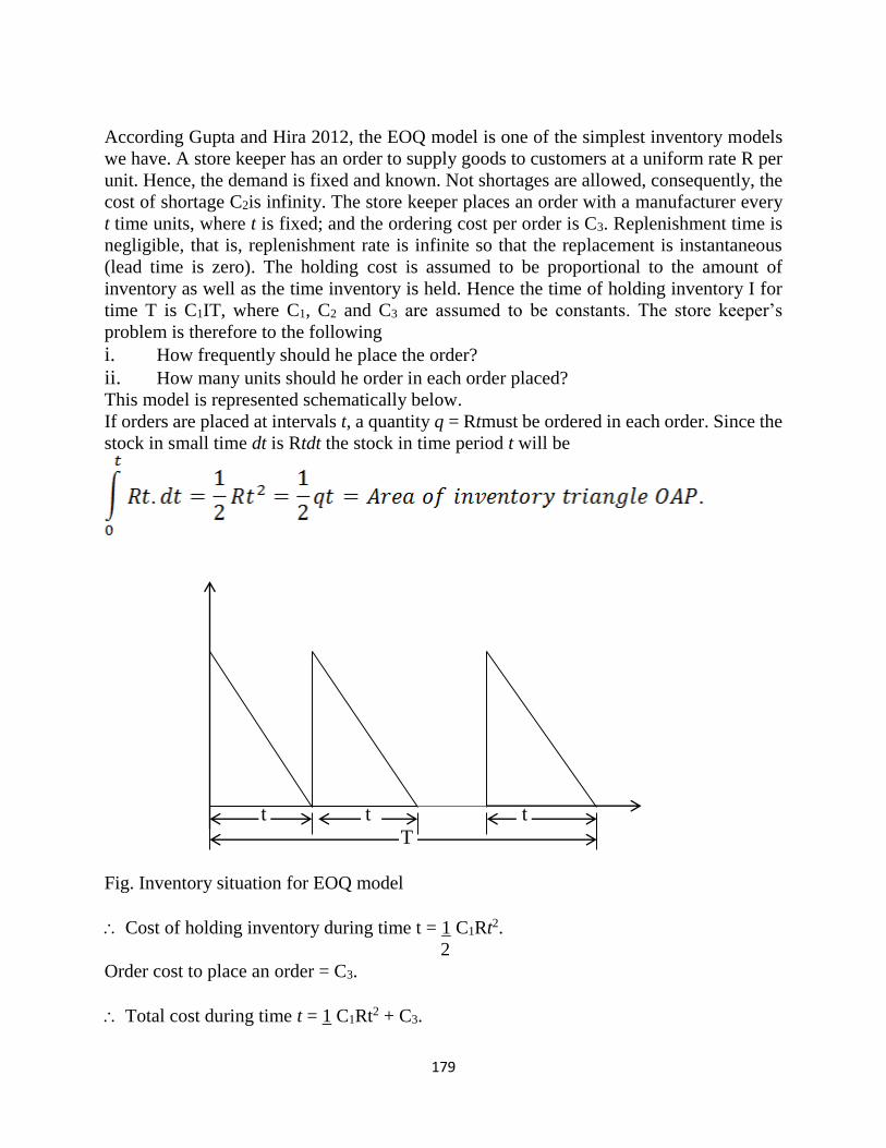
179

According Gupta and Hira 2012, the EOQ model is one of the simplest inventory models

we have. A store keeper has an order to supply goods to customers at a uniform rate R per

unit. Hence, the demand is fixed and known. Not shortages are allowed, consequently, the

cost of shortage C2is infinity. The store keeper places an order with a manufacturer every

t time units, where t is fixed; and the ordering cost per order is C3. Replenishment time is

negligible, that is, replenishment rate is infinite so that the replacement is instantaneous

(lead time is zero). The holding cost is assumed to be proportional to the amount of

inventory as well as the time inventory is held. Hence the time of holding inventory I for

time T is C1IT, where C1, C2 and C3 are assumed to be constants. The store keeper’s

problem is therefore to the following

i. How frequently should he place the order?

ii. How many units should he order in each order placed?

This model is represented schematically below.

If orders are placed at intervals t, a quantity q = Rtmust be ordered in each order. Since the

stock in small time dt is Rtdt the stock in time period t will be

t t t

T

Fig. Inventory situation for EOQ model

Cost of holding inventory during time t = 1 C1Rt2.

2

Order cost to place an order = C3.

Total cost during time t = 1 C1Rt2 + C3.

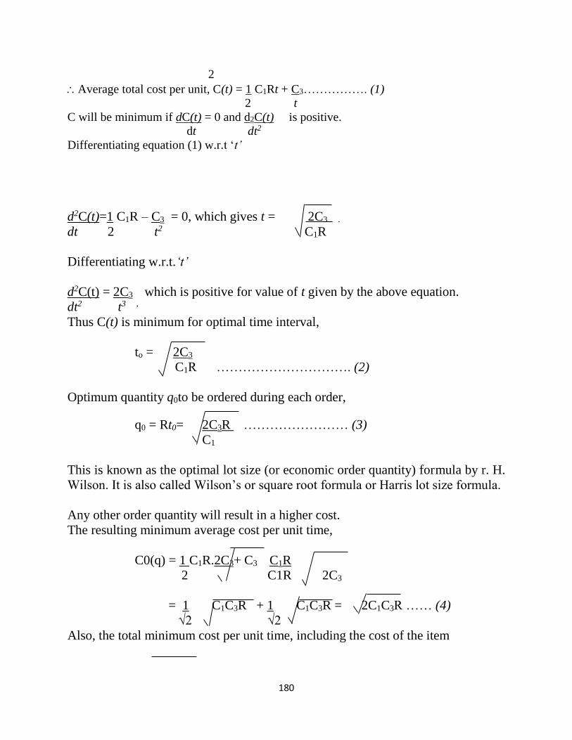
180

2

Average total cost per unit, C(t) = 1 C1Rt + C3……………. (1)

2 t

C will be minimum if dC(t) = 0 and d2C(t) is positive.

dt dt2

Differentiating equation (1) w.r.t ‘t’

d2C(t)=1 C1R – C3 = 0, which gives t = 2C3 .

dt 2 t2 C1R

Differentiating w.r.t.‘t’

d2C(t) = 2C3 which is positive for value of t given by the above equation.

dt2 t3 ,

Thus C(t) is minimum for optimal time interval,

to = 2C3

C1R …………………………. (2)

Optimum quantity q0to be ordered during each order,

q0 = Rt0= 2C3R …………………… (3)

C1

This is known as the optimal lot size (or economic order quantity) formula by r. H.

Wilson. It is also called Wilson’s or square root formula or Harris lot size formula.

Any other order quantity will result in a higher cost.

The resulting minimum average cost per unit time,

C0(q) = 1 C1R.2C3+ C3 C1R

2 C1R 2C3

= 1 C1C3R + 1 C1C3R = 2C1C3R …… (4)

√2 √2

Also, the total minimum cost per unit time, including the cost of the item

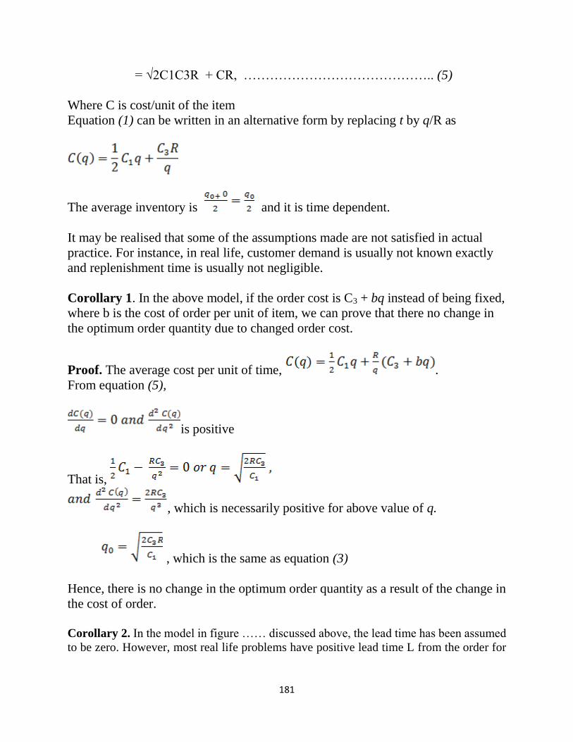
181

= √2C1C3R + CR, …………………………………….. (5)

Where C is cost/unit of the item

Equation (1) can be written in an alternative form by replacing t by q/R as

The average inventory is and it is time dependent.

It may be realised that some of the assumptions made are not satisfied in actual

practice. For instance, in real life, customer demand is usually not known exactly

and replenishment time is usually not negligible.

Corollary 1. In the above model, if the order cost is C3 + bq instead of being fixed,

where b is the cost of order per unit of item, we can prove that there no change in

the optimum order quantity due to changed order cost.

Proof. The average cost per unit of time, .

From equation (5),

is positive

That is,

, which is necessarily positive for above value of q.

, which is the same as equation (3)

Hence, there is no change in the optimum order quantity as a result of the change in

the cost of order.

Corollary 2. In the model in figure …… discussed above, the lead time has been assumed

to be zero. However, most real life problems have positive lead time L from the order for

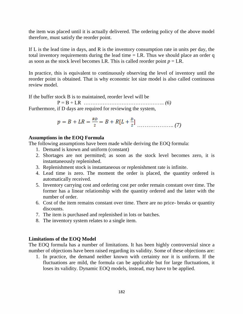
182

the item was placed until it is actually delivered. The ordering policy of the above model

therefore, must satisfy the reorder point.

If L is the lead time in days, and R is the inventory consumption rate in units per day, the

total inventory requirements during the lead time = LR. Thus we should place an order q

as soon as the stock level becomes LR. This is called reorder point p = LR.

In practice, this is equivalent to continuously observing the level of inventory until the

reorder point is obtained. That is why economic lot size model is also called continuous

review model.

If the buffer stock B is to maintained, reorder level will be

P = B + LR ……………………………………….. (6)

Furthermore, if D days are required for reviewing the system,

……………….. (7)

Assumptions in the EOQ Formula

The following assumptions have been made while deriving the EOQ formula:

1. Demand is known and uniform (constant)

2. Shortages are not permitted; as soon as the stock level becomes zero, it is

instantaneously replenished.

3. Replenishment stock is instantaneous or replenishment rate is infinite.

4. Lead time is zero. The moment the order is placed, the quantity ordered is

automatically received.

5. Inventory carrying cost and ordering cost per order remain constant over time. The

former has a linear relationship with the quantity ordered and the latter with the

number of order.

6. Cost of the item remains constant over time. There are no price- breaks or quantity

discounts.

7. The item is purchased and replenished in lots or batches.

8. The inventory system relates to a single item.

Limitations of the EOQ Model

The EOQ formula has a number of limitations. It has been highly controversial since a

number of objections have been raised regarding its validity. Some of these objections are:

1. In practice, the demand neither known with certainty nor it is uniform. If the

fluctuations are mild, the formula can be applicable but for large fluctuations, it

loses its validity. Dynamic EOQ models, instead, may have to be applied.

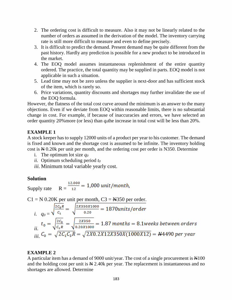
183

2. The ordering cost is difficult to measure. Also it may not be linearly related to the

number of orders as assumed in the derivation of the model. The inventory carrying

rate is still more difficult to measure and even to define precisely.

3. It is difficult to predict the demand. Present demand may be quite different from the

past history. Hardly any prediction is possible for a new product to be introduced in

the market.

4. The EOQ model assumes instantaneous replenishment of the entire quantity

ordered. The practice, the total quantity may be supplied in parts. EOQ model is not

applicable in such a situation.

5. Lead time may not be zero unless the supplier is next-door and has sufficient stock

of the item, which is rarely so.

6. Price variations, quantity discounts and shortages may further invalidate the use of

the EOQ formula.

However, the flatness of the total cost curve around the minimum is an answer to the many

objections. Even if we deviate from EOQ within reasonable limits, there is no substantial

change in cost. For example, if because of inaccuracies and errors, we have selected an

order quantity 20%more (or less) than q0the increase in total cost will be less than 20%.

EXAMPLE 1

A stock keeper has to supply 12000 units of a product per year to his customer. The demand

is fixed and known and the shortage cost is assumed to be infinite. The inventory holding

cost is N 0.20k per unit per month, and the ordering cost per order is N350. Determine

i. The optimum lot size q0

ii. Optimum scheduling period t0

iii. Minimum total variable yearly cost.

Solution

Supply rate R =

C1 = N 0.20K per unit per month, C3 = N350 per order.

i. q0 =

ii.

iii.

EXAMPLE 2

A particular item has a demand of 9000 unit/year. The cost of a single procurement is N100

and the holding cost per unit is N 2.40k per year. The replacement is instantaneous and no

shortages are allowed. Determine

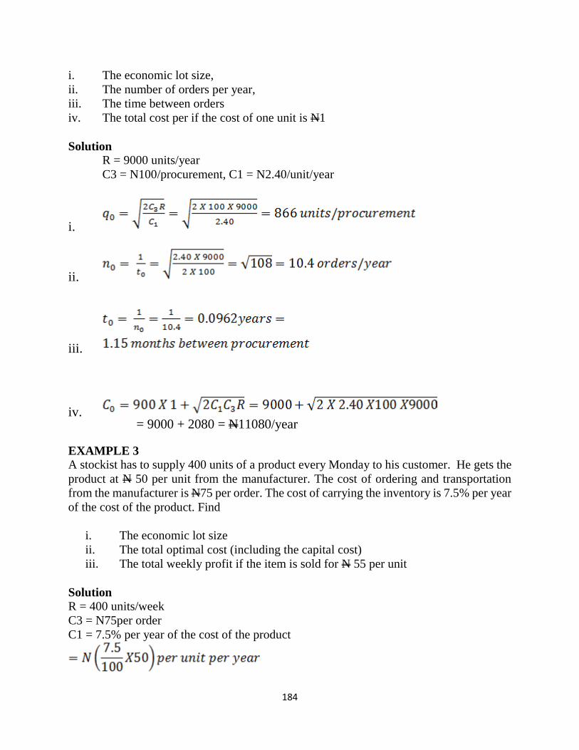
184

i. The economic lot size,

ii. The number of orders per year,

iii. The time between orders

iv. The total cost per if the cost of one unit is N1

Solution

R = 9000 units/year

C3 = N100/procurement, C1 = N2.40/unit/year

i.

ii.

iii.

iv. = 9000 + 2080 = N11080/year

EXAMPLE 3

A stockist has to supply 400 units of a product every Monday to his customer. He gets the

product at N 50 per unit from the manufacturer. The cost of ordering and transportation

from the manufacturer is N75 per order. The cost of carrying the inventory is 7.5% per year

of the cost of the product. Find

i. The economic lot size

ii. The total optimal cost (including the capital cost)

iii. The total weekly profit if the item is sold for N 55 per unit

Solution

R = 400 units/week

C3 = N75per order

C1 = 7.5% per year of the cost of the product

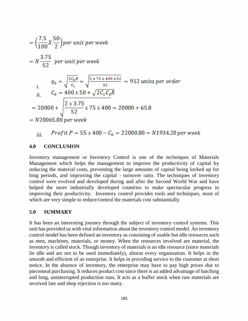
185

i.

ii.

iii.

4.0 CONCLUSION







improving their productivity. Inventory control provides tools and techniques, most of

which are very simple to reduce/control the materials cost substantially.

5.0 SUMMARY

It has been an interesting journey through the subject of inventory control systems. This

unit has provided us with vital information about the inventory control model. An inventory

control model has been defined an inventory as consisting of usable but idle resources such


inventory is called stock. Though inventory of materials is an idle resource (since materials

lie idle and are not to be used immediately), almost every organisation. It helps in the

smooth and efficient of an enterprise. It helps in providing service to the customer at short

notice. In the absence of inventory, the enterprise may have to pay high prices due to

piecemeal purchasing. It reduces product cost since there is an added advantage of batching

and long, uninterrupted production runs. It acts as a buffer stock when raw materials are

received late and shop rejection is too many.

186


What do you understand by the term inventory control?

Identify and discuss the different classifications of inventories.

Give six limitations of the EOQ model.

Outline the assumptions of the EOQ formula

8.0 REFERENCES

Eiselt, H.A., and Sandblom, C.L. (2012). Operations Research: A Model Based

Approach, 2nd ed., NewYork:Springer Heidelberg


Company.


Nigeria.

187

UNIT 14: SEQUENCING

1.0 Introduction

2.0 Objectives

3.0 Main Content

3.1 The Problem:(Definition)

3.2 Assumptions Made in Sequencing Problems

3.3 Nature of Scheduling

3.4 Loading Jobs in Work Centres

3.4.1 Gantt Charts

3.4.2 Assignment Method

3.5 Priority Rules for Job Sequencing

3.6 Applicability

3.7 Types of Sequencing Problems

3.7.1 Sequencing Jobs in two Machines

4.0 Conclusion

5.0 Summary


7.0 References

1.0 INTRODUCTION

Sequencing problems involves the determination of an optimal order or sequence of

performing a series jobs by number of facilities (that are arranged in specific order) so as

to optimize the total time or cost. Sequencing problems can be classified into two groups:

The group involves n different jobs to be performed, and these jobs require processing on

some or all of m different types of machines. The order in which these machines are to be

used for processing each job (for example, each job is to be processed first on machine A,

then B, and thereafter on C i.e., in the order ABC) is given. Also, the expected actual

processing time of each job on each machine is known. We can also determine the

effectiveness for any given sequence of jobs on each of the machines and we wish to select

from the (n!)m theoretically feasible alternatives, the one which is both technologically

feasible and optimises the effectiveness measure.

188

2.0 OBJECTIVES

After completing this chapter, you should be able to:

1. Explain what scheduling involves and the nature of scheduling.

2. Understand the use of Gantt charts and assignment method for loading jobs in work

centres.

3. Discuss what sequencing involves and the use of priority rules.

4. Solve simple problems on scheduling and sequencing.

3.0 MAIN CONTENT

3.1 DEFINITION

Scheduling refers to establishing the timing of the use of equipment, facilities and human

activities in an organization, that is, it deals with the timing of operations. Scheduling

occurs in every organization, regardless of the nature of its operation. For example,

manufacturing organizations, hospitals, colleges, airlines e.t.c. schedule their activities to

achieve greater efficiency. Effective Scheduling helps companies to use assets more

efficiently, which leads to cost savings and increase in productivity. The flexibility in

operation provides faster delivery and therefore, better customer service. In general, the

objectives of scheduling are to achieve trade-offs among conflicting goals, which include

efficient utilization of staff, equipment and facilities and minimization of customer waiting

tune, inventories and process times (Adebayo et al, 2006).

3.2 ASSUMPTIONS MADE IN SEQUENCING PROBLEMS

Principal assumptions made for convenience in solving the sequencing problems are as

follows:

1. The processing times Ai and Bi etc. are exactly known to us and they are independent of

order of processing the job on the machine. That is whether job is done first on the machine,

last on the machine, the time taken to process the job will not vary it remains constant.

2. The time taken by the job from one machine to other after processing on the previous

machine is negligible. (Or we assume that the processing time given also includes the

transfer time and setup time).

3. Only one operation can be carried out on a machine at a particular time.

4. Each job once started on the machine, we should not stop the processing in the middle.

It is to be processed completely before loading the next job.

5. The job starts on the machine as soon as the job and the machine both become idle

(vacant). This is written as job is next to the machine and the machine is next to the job.

(This is exactly the meaning of transfer time is negligible).

3.3 NATURE OF SCHEDULING

Scheduling technique depends on the volume of system output, the nature of operations

and the overall complexity of jobs. Flow shop systems require approaches substantially

189

different from those required by job shops. The complexity of operations varies under these

two situations.

1. Flow Shop

Flow shop is a high-volume system, which is characterized by a continuous flow of jobs to

produce standardized products. Also, flow shop uses standardized equipment (i.e. special

purposed machines) and activities that provide mass production. The goal is to obtain a

smooth rate of flow of goods or customer through the system in order to get high utilization

of labour and equipment. Examples are refineries, production of detergents etc.

2. Job Shop

This is a low volume system, which periodically shift from one job to another. The

production is according to customer’s specifications and orders or jobs usually in small

lots. General-purpose machines characterize Job shop. For example, in designer shop, a

customer can place order for different design.

Job-shop processing gives rise to two basic issues for schedulers: how to distribute the

workload among work centre and what job processing sequence to use.

3.4 LOADING JOBS IN WORK CENTRES

Loading refers to the assignment of jobs to work centres. The operation managers are

confronted with the decision of assigning jobs to work centres to minimize costs, idle time

or completion time.

The two main methods that can be used to assign jobs to work centres or to allocate

resources are:

1. Gantt chart

2. Assignment method of linear programming

3.4.1 Gantt Charts

Gantt charts are bar charts that show the relationship of activities over some time periods.

Gantt charts are named after Henry Gantt, the pioneer who used charts for industrial

scheduling in the early 1900s. A typical Gantt chart presents time scale horizontally, and

resources to be scheduled are listed vertically, the use and idle times of resources are

reflected in the chart.

The two most commonly used Gantt charts are the schedule chart and the load chart.

3.4.2 Assignment Method

Assignment Model (AM) is concerned specifically with the problem of job allocation in a

multiple facility production configuration. That is, it is useful in situations that call for

assigning tasks or jobs to resources. Typical examples include assigning jobs to machines

or workers, territories to sales people e.t.c. One important characteristic of assignment

problems is that only one job (or worker) is assigned to one machine (or project). The idea

is to obtain an optimum matching of tasks and resources. A chapter in this book has treated

the assignment method.

190

3.5 PRIORITY RULES FOR JOB SEQUENCING

Priority rules provide means for selecting the order in which jobs should be done

(processed). In using these rules, it is assumed that job set up cost and time are independent

of processing sequence. The main objective of priority rules is to minimize completion

time, number of jobs in the system, and job lateness, while maximizing facility utilization.

The most popular priority rules are:

I. First Come, First Serve (FCFS): Job is worked or processed in the order of arrivals at the

work centre.

2. Shortest Processing Time (SPT): Here, jobs are processed based on the length of

processing time. The job with the least processing time is done first.

3. Earliest Due Date (EDD): This rule sequences jobs according to their due dates, that is,

the job with the earliest due date is processed first.

4. Longest Processing Time (LPT): The job with the longest processing time is started first.

5. Critical Ratio: Jobs are processed according to smallest ratio of time remaining until due

date to processing time remaining.

The effectiveness of the priority rules is frequently measured in the light of one or more

performance measures namely; average number of jobs, job flow time, job lateness, make

span, facility utilisation etc.

3.6 APPLICABILITY

The sequencing problem is very much common in Job workshops and Batch production

shops. There will be number of jobs which are to be processed on a series of machine in a

specified order depending on the physical changes required on the job. We can find the

same situation in computer centre where

number of problems waiting for a solution. We can also see the same situation when

number of critical patients waiting for treatment in a clinic and in Xerox centres, where

number of jobs is in queue, which are to be processed on the Xerox machines. Like this we

may find number of situations in real world.

3.7 TYPES OF SEQUENCING PROBLEMS

There are various types of sequencing problems arise in real world. All sequencing

problems cannot be solved. Though mathematicians and Operations Research scholars are

working hard on the problem satisfactory method of solving problem is available for few

cases only. The problems, which can be

solved, are:

(a) ‘n’ jobs are to be processed on two machines say machine A and machine B in the

order AB. This means that the job is to be processed first on machine A and then on

machine B.

(b) ‘n’ jobs are to be processed on three machines A,B and C in the order ABC i.e. first

on machine A, second on machine B and third on machine C.

(c) ‘n’ jobs are to be processed on ‘m’ machines in the given order.

d) Two jobs are to be processed on ‘m’ machines in the given order. (Murthy, 2007)

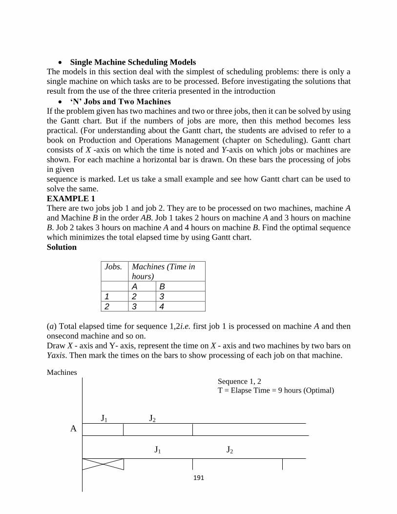
191

Single Machine Scheduling Models

The models in this section deal with the simplest of scheduling problems: there is only a

single machine on which tasks are to be processed. Before investigating the solutions that

result from the use of the three criteria presented in the introduction

‘N’ Jobs and Two Machines

If the problem given has two machines and two or three jobs, then it can be solved by using

the Gantt chart. But if the numbers of jobs are more, then this method becomes less

practical. (For understanding about the Gantt chart, the students are advised to refer to a

book on Production and Operations Management (chapter on Scheduling). Gantt chart

consists of X -axis on which the time is noted and Y-axis on which jobs or machines are

shown. For each machine a horizontal bar is drawn. On these bars the processing of jobs

in given

sequence is marked. Let us take a small example and see how Gantt chart can be used to

solve the same.

EXAMPLE 1

There are two jobs job 1 and job 2. They are to be processed on two machines, machine A

and Machine B in the order AB. Job 1 takes 2 hours on machine A and 3 hours on machine

B. Job 2 takes 3 hours on machine A and 4 hours on machine B. Find the optimal sequence

which minimizes the total elapsed time by using Gantt chart.

Solution

Jobs. Machines (Time in

hours)

A B

1 2 3

2 3 4

(a) Total elapsed time for sequence 1,2i.e. first job 1 is processed on machine A and then

onsecond machine and so on.

Draw X - axis and Y- axis, represent the time on X - axis and two machines by two bars on

Yaxis. Then mark the times on the bars to show processing of each job on that machine.

Machines

Sequence 1, 2

T = Elapse Time = 9 hours (Optimal)

J1 J2

A

J1 J2

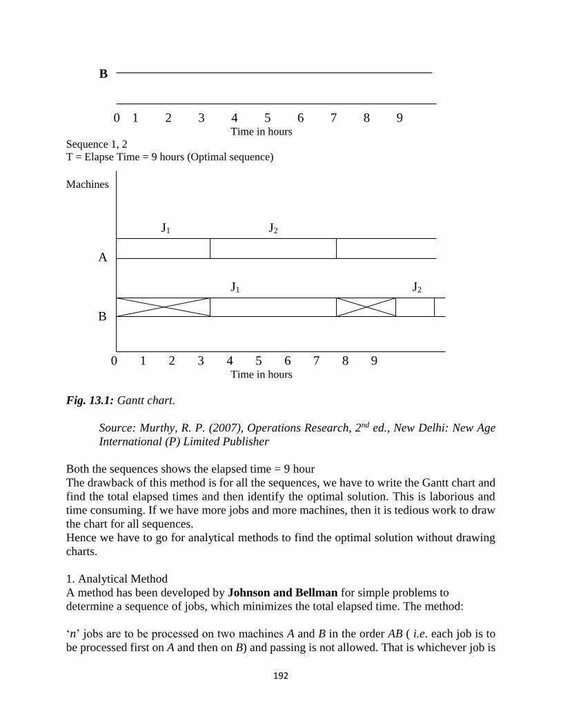
192

B

0 1 2 3 4 5 6 7 8 9 Time in hours

Sequence 1, 2

T = Elapse Time = 9 hours (Optimal sequence) Machines

J1 J2

A

J1 J2

B

0 1 2 3 4 5 6 7 8 9 Time in hours

Fig. 13.1: Gantt chart.

Source: Murthy, R. P. (2007), Operations Research, 2nd ed., New Delhi: New Age

International (P) Limited Publisher

Both the sequences shows the elapsed time = 9 hour

The drawback of this method is for all the sequences, we have to write the Gantt chart and

find the total elapsed times and then identify the optimal solution. This is laborious and

time consuming. If we have more jobs and more machines, then it is tedious work to draw

the chart for all sequences.

Hence we have to go for analytical methods to find the optimal solution without drawing

charts.

1. Analytical Method

A method has been developed by Johnson and Bellman for simple problems to

determine a sequence of jobs, which minimizes the total elapsed time. The method:

‘n’ jobs are to be processed on two machines A and B in the order AB ( i.e. each job is to

be processed first on A and then on B) and passing is not allowed. That is whichever job is

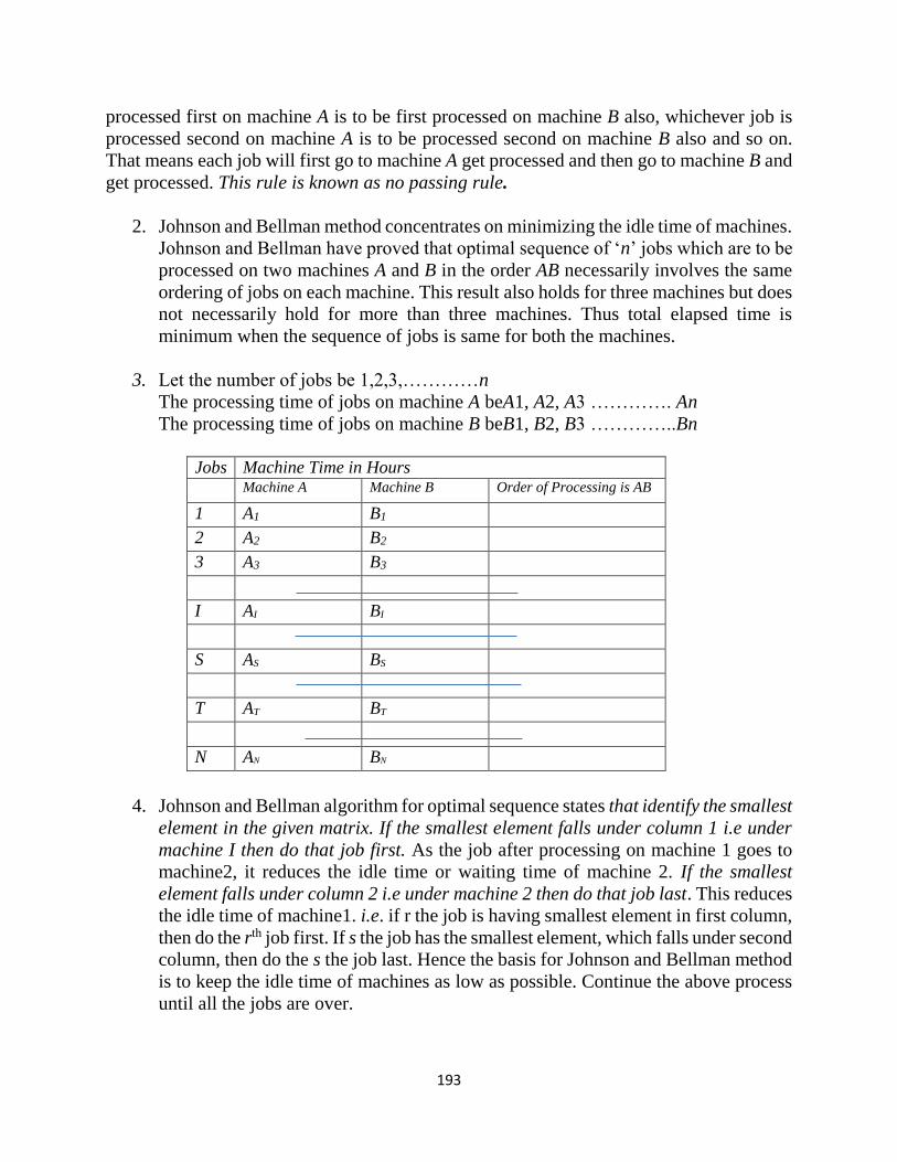
193

processed first on machine A is to be first processed on machine B also, whichever job is

processed second on machine A is to be processed second on machine B also and so on.

That means each job will first go to machine A get processed and then go to machine B and

get processed. This rule is known as no passing rule.

2. Johnson and Bellman method concentrates on minimizing the idle time of machines.

Johnson and Bellman have proved that optimal sequence of ‘n’ jobs which are to be

processed on two machines A and B in the order AB necessarily involves the same

ordering of jobs on each machine. This result also holds for three machines but does

not necessarily hold for more than three machines. Thus total elapsed time is

minimum when the sequence of jobs is same for both the machines.

3. Let the number of jobs be 1,2,3,…………n

The processing time of jobs on machine A beA1, A2, A3 …………. An

The processing time of jobs on machine B beB1, B2, B3 …………..Bn

Jobs Machine Time in Hours

Machine A Machine B Order of Processing is AB

1 A1 B1 2 A2 B2 3 A3 B3

I AI BI S AS BS T AT BT N AN BN

4. Johnson and Bellman algorithm for optimal sequence states that identify the smallest

element in the given matrix. If the smallest element falls under column 1 i.e under

machine I then do that job first. As the job after processing on machine 1 goes to

machine2, it reduces the idle time or waiting time of machine 2. If the smallest

element falls under column 2 i.e under machine 2 then do that job last. This reduces

the idle time of machine1. i.e. if r the job is having smallest element in first column,

then do the rth job first. If s the job has the smallest element, which falls under second

column, then do the s the job last. Hence the basis for Johnson and Bellman method

is to keep the idle time of machines as low as possible. Continue the above process

until all the jobs are over.

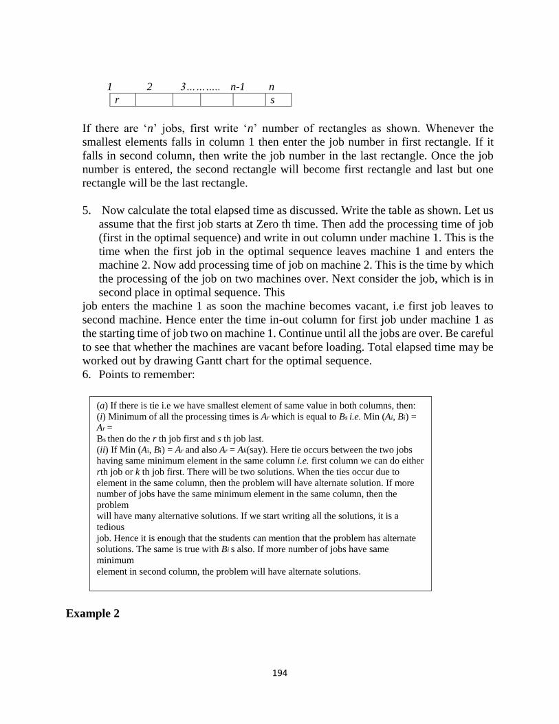
194

1 2 3……….. n-1 n

r s

If there are ‘n’ jobs, first write ‘n’ number of rectangles as shown. Whenever the

smallest elements falls in column 1 then enter the job number in first rectangle. If it

falls in second column, then write the job number in the last rectangle. Once the job

number is entered, the second rectangle will become first rectangle and last but one

rectangle will be the last rectangle.

5. Now calculate the total elapsed time as discussed. Write the table as shown. Let us

assume that the first job starts at Zero th time. Then add the processing time of job

(first in the optimal sequence) and write in out column under machine 1. This is the

time when the first job in the optimal sequence leaves machine 1 and enters the

machine 2. Now add processing time of job on machine 2. This is the time by which

the processing of the job on two machines over. Next consider the job, which is in

second place in optimal sequence. This

job enters the machine 1 as soon the machine becomes vacant, i.e first job leaves to

second machine. Hence enter the time in-out column for first job under machine 1 as

the starting time of job two on machine 1. Continue until all the jobs are over. Be careful

to see that whether the machines are vacant before loading. Total elapsed time may be

worked out by drawing Gantt chart for the optimal sequence.

6. Points to remember:

Example 2

(a) If there is tie i.e we have smallest element of same value in both columns, then:

(i) Minimum of all the processing times is Ar which is equal to Bs i.e. Min (Ai, Bi) =

Ar =

Bs then do the r th job first and s th job last.

(ii) If Min (Ai, Bi) = Ar and also Ar = Ak(say). Here tie occurs between the two jobs

having same minimum element in the same column i.e. first column we can do either

rth job or k th job first. There will be two solutions. When the ties occur due to

element in the same column, then the problem will have alternate solution. If more

number of jobs have the same minimum element in the same column, then the

problem

will have many alternative solutions. If we start writing all the solutions, it is a

tedious

job. Hence it is enough that the students can mention that the problem has alternate

solutions. The same is true with Bi s also. If more number of jobs have same

minimum

element in second column, the problem will have alternate solutions.

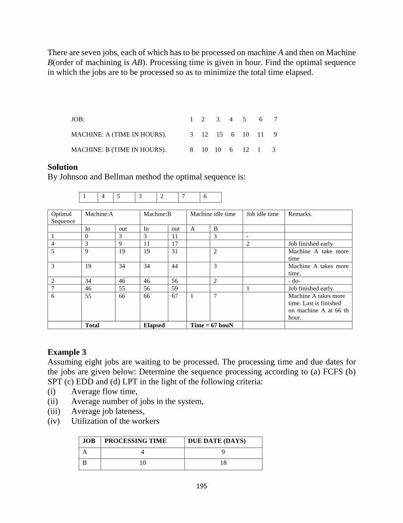
195

There are seven jobs, each of which has to be processed on machine A and then on Machine

B(order of machining is AB). Processing time is given in hour. Find the optimal sequence

in which the jobs are to be processed so as to minimize the total time elapsed.

JOB: 1 2 3 4 5 6 7

MACHINE: A (TIME IN HOURS). 3 12 15 6 10 11 9

MACHINE: B (TIME IN HOURS). 8 10 10 6 12 1 3

Solution

By Johnson and Bellman method the optimal sequence is:

1 4 5 3 2 7 6

Optimal

Sequence

Machine:A Machine:B Machine idle time Job idle time Remarks.

In out In out A B

1 0 3 3 11 3 -

4 3 9 11 17 2 Job finished early

5 9 19 19 31 2 Machine A take more

time

3 19 34 34 44 3 Machine A takes more

time.

2 34 46 46 56 2 - do-

7 46 55 56 59 1 Job finished early.

6 55 66 66 67 1 7 Machine A takes more

time. Last is finished

on machine A at 66 th

hour.

Total Elapsed Time = 67 houN

Example 3

Assuming eight jobs are waiting to be processed. The processing time and due dates for

the jobs are given below: Determine the sequence processing according to (a) FCFS (b)

SPT (c) EDD and (d) LPT in the light of the following criteria:

(i) Average flow time,

(ii) Average number of jobs in the system,

(iii) Average job lateness,

(iv) Utilization of the workers

JOB PROCESSING TIME DUE DATE (DAYS)

A 4 9

B 10 18

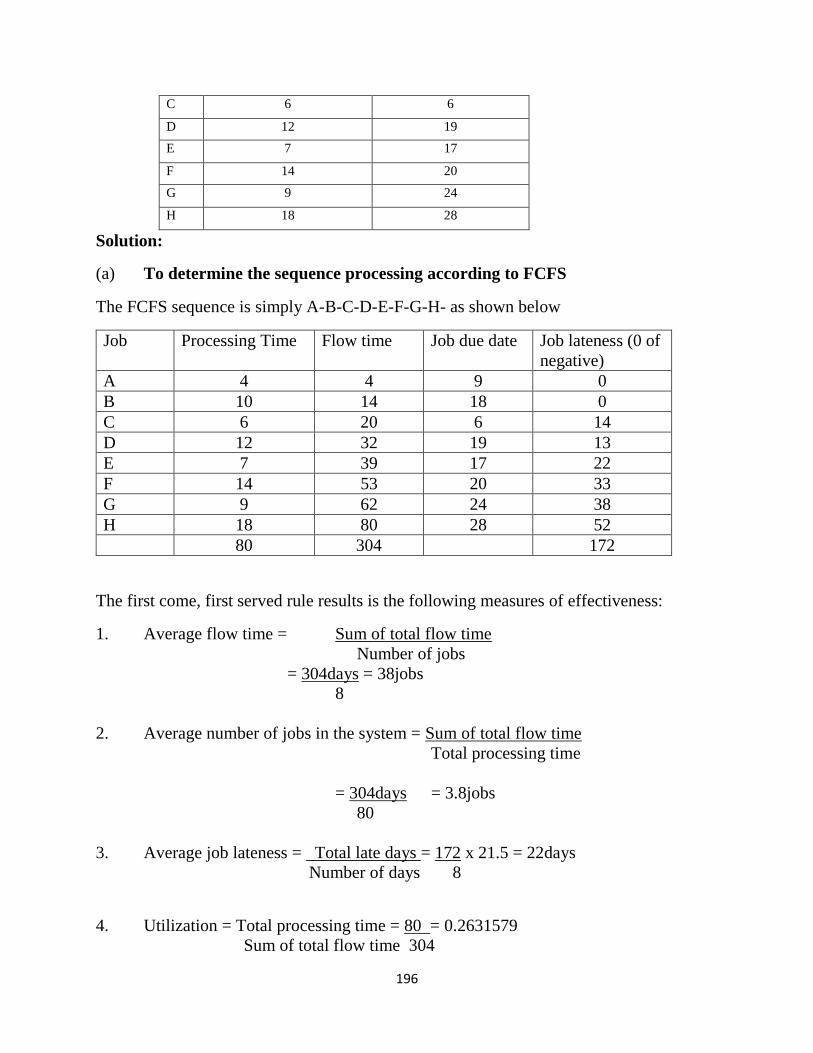
196

C 6 6

D 12 19

E 7 17

F 14 20

G 9 24

H 18 28

Solution:

(a) To determine the sequence processing according to FCFS

The FCFS sequence is simply A-B-C-D-E-F-G-H- as shown below

Job Processing Time Flow time Job due date Job lateness (0 of

negative)

A 4 4 9 0

B 10 14 18 0

C 6 20 6 14

D 12 32 19 13

E 7 39 17 22

F 14 53 20 33

G 9 62 24 38

H 18 80 28 52

80 304 172

The first come, first served rule results is the following measures of effectiveness:

1. Average flow time = Sum of total flow time

Number of jobs

= 304days = 38jobs

8

2. Average number of jobs in the system = Sum of total flow time

Total processing time

= 304days = 3.8jobs

80

3. Average job lateness = Total late days = 172 x 21.5 = 22days

Number of days 8

4. Utilization = Total processing time = 80 = 0.2631579

Sum of total flow time 304

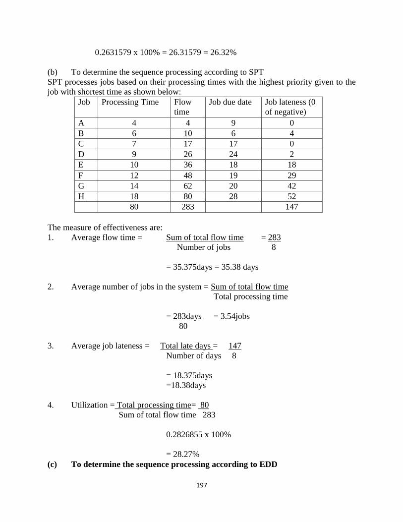
197

0.2631579 x 100% = 26.31579 = 26.32%

(b) To determine the sequence processing according to SPT

SPT processes jobs based on their processing times with the highest priority given to the

job with shortest time as shown below:

Job Processing Time Flow

time

Job due date Job lateness (0

of negative)

A 4 4 9 0

B 6 10 6 4

C 7 17 17 0

D 9 26 24 2

E 10 36 18 18

F 12 48 19 29

G 14 62 20 42

H 18 80 28 52

80 283 147

The measure of effectiveness are:

1. Average flow time = Sum of total flow time = 283

Number of jobs 8

= 35.375days = 35.38 days

2. Average number of jobs in the system = Sum of total flow time

Total processing time

= 283days = 3.54jobs

80

3. Average job lateness = Total late days = 147

Number of days 8

= 18.375days

=18.38days

4. Utilization = Total processing time= 80

Sum of total flow time 283

0.2826855 x 100%

= 28.27%

(c) To determine the sequence processing according to EDD

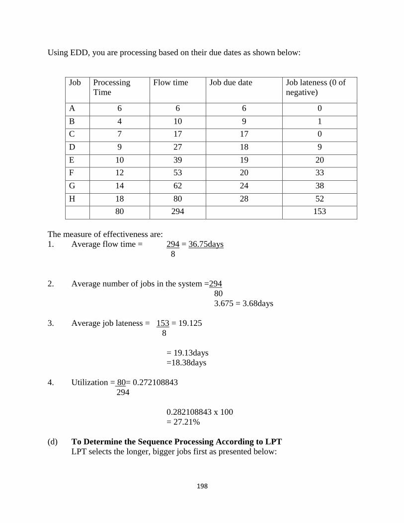
198

Using EDD, you are processing based on their due dates as shown below:

Job Processing

Time

Flow time Job due date Job lateness (0 of

negative)

A 6 6 6 0

B 4 10 9 1

C 7 17 17 0

D 9 27 18 9

E 10 39 19 20

F 12 53 20 33

G 14 62 24 38

H 18 80 28 52

80 294 153


1. Average flow time = 294 = 36.75days

8

2. Average number of jobs in the system =294

80

3.675 = 3.68days

3. Average job lateness = 153 = 19.125

8

= 19.13days

=18.38days

4. Utilization = 80= 0.272108843

294

0.282108843 x 100

= 27.21%

(d) To Determine the Sequence Processing According to LPT

LPT selects the longer, bigger jobs first as presented below:

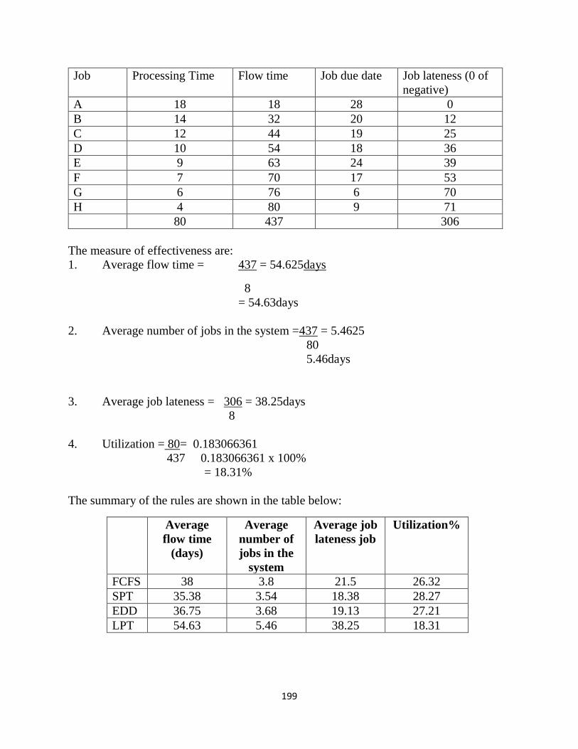
199

Job Processing Time Flow time Job due date Job lateness (0 of

negative)

A 18 18 28 0

B 14 32 20 12

C 12 44 19 25

D 10 54 18 36

E 9 63 24 39

F 7 70 17 53

G 6 76 6 70

H 4 80 9 71

80 437 306


1. Average flow time = 437 = 54.625days

8

= 54.63days

2. Average number of jobs in the system =437 = 5.4625

80

5.46days

3. Average job lateness = 306 = 38.25days

8

4. Utilization = 80= 0.183066361

437 0.183066361 x 100%

= 18.31%

The summary of the rules are shown in the table below:

Average

flow time

(days)

Average

number of

jobs in the

system

Average job

lateness job

Utilization%

FCFS 38 3.8 21.5 26.32

SPT 35.38 3.54 18.38 28.27

EDD 36.75 3.68 19.13 27.21

LPT 54.63 5.46 38.25 18.31

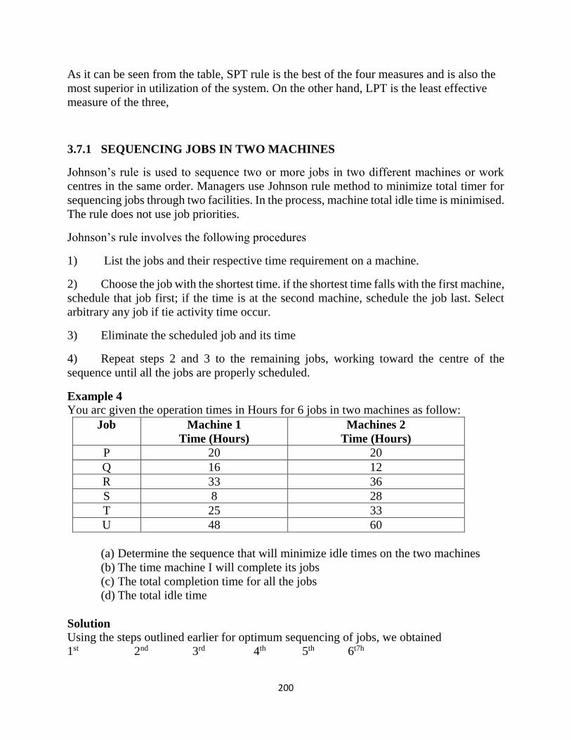
200

As it can be seen from the table, SPT rule is the best of the four measures and is also the

most superior in utilization of the system. On the other hand, LPT is the least effective

measure of the three,

3.7.1 SEQUENCING JOBS IN TWO MACHINES

Johnson’s rule is used to sequence two or more jobs in two different machines or work

centres in the same order. Managers use Johnson rule method to minimize total timer for

sequencing jobs through two facilities. In the process, machine total idle time is minimised.

The rule does not use job priorities.

Johnson’s rule involves the following procedures

1) List the jobs and their respective time requirement on a machine.

2) Choose the job with the shortest time. if the shortest time falls with the first machine,

schedule that job first; if the time is at the second machine, schedule the job last. Select

arbitrary any job if tie activity time occur.

3) Eliminate the scheduled job and its time

4) Repeat steps 2 and 3 to the remaining jobs, working toward the centre of the

sequence until all the jobs are properly scheduled.

Example 4

You arc given the operation times in Hours for 6 jobs in two machines as follow:

Job Machine 1

Time (Hours)

Machines 2

Time (Hours)

P 20 20

Q 16 12

R 33 36

S 8 28

T 25 33

U 48 60

(a) Determine the sequence that will minimize idle times on the two machines

(b) The time machine I will complete its jobs

(c) The total completion time for all the jobs

(d) The total idle time

Solution

Using the steps outlined earlier for optimum sequencing of jobs, we obtained

1st 2nd 3rd 4th 5th 6t7h

201

S T R U E Q

We then use tabular method to solve the remaining questions

Job

sequence

1

Machine

1

Duration

II

Machine

1 in

III

Machine

I Out

IV

Machine

2

Duration

V

Machine

2 In

VI

Machines

2 Out

VII

Idle

Time

S 8 0 8 28 8 36 8

T 25 8 33 33 36 69 0

R 33 33 66 36 69 105 0

U 48 66 114 60 114 174 9

P 20 114 134 20 174 194 0

Q 16 134 150 12 194 206 0

(a) Machine 1 will complete his job in150 hours

(b) Total completion time is 206 hours

(c) Total idle time is 17 hours

Note that machine 2 will wait 8 hours for its first job and also wait 9 hours after completing

job R.

In general, idle time can occur either at the beginning of job or at the end of sequence of

jobs. In manufacturing organizations, idle times can be used to do other jobs like

maintenance, dismantling or setting up of other equipment.

4.0 CONCLUSION

Sequencing problems involves the determination of an optimal order or sequence of

performing a series jobs by number of facilities (that are arranged in specific order) so as

to optimize the total time or cost. Sequencing problems can be classified into two groups.

The first group involves n different jobs to be performed, and these jobs require processing

on some or all of m different types of machines. The order in which these machines are to

be used for processing each job (for example, each job is to be processed first on machine

A, then B, and thereafter on C i.e., in the order ABC) is given.

5.0 SUMMARY

Scheduling, which occurs in every organisation, refers to establishing the timing of the use

of equipment, facilities and human activities in an organization and so it deals with the

timing of operations. Scheduling technique depends on the volume of system output, the

nature of operations and the overall complexity of jobs. The complexity of operation varies

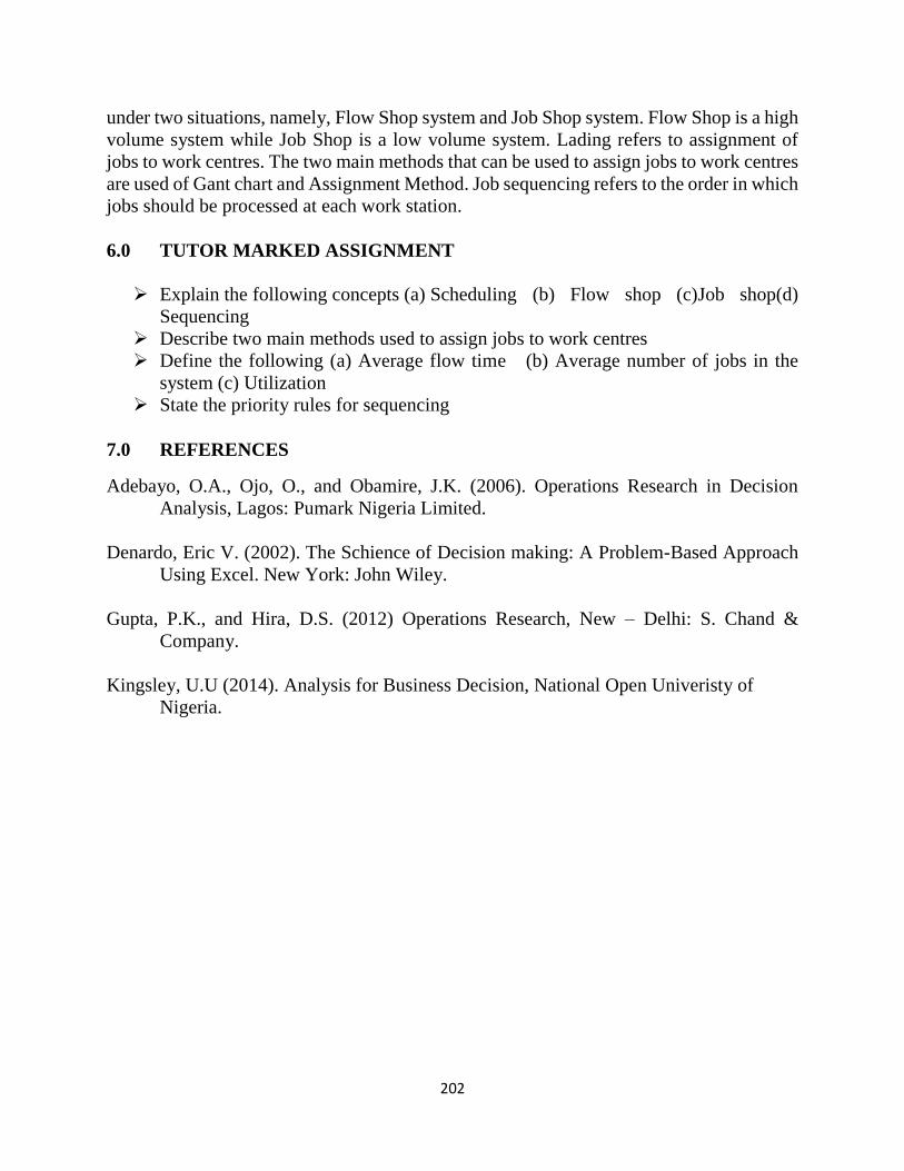
202

under two situations, namely, Flow Shop system and Job Shop system. Flow Shop is a high

volume system while Job Shop is a low volume system. Lading refers to assignment of

jobs to work centres. The two main methods that can be used to assign jobs to work centres

are used of Gant chart and Assignment Method. Job sequencing refers to the order in which

jobs should be processed at each work station.


Explain the following concepts (a) Scheduling (b) Flow shop (c)Job shop(d)

Sequencing

Describe two main methods used to assign jobs to work centres

Define the following (a) Average flow time (b) Average number of jobs in the

system (c) Utilization

State the priority rules for sequencing

7.0 REFERENCES

Adebayo, O.A., Ojo, O., and Obamire, J.K. (2006). Operations Research in Decision


Denardo, Eric V. (2002). The Schience of Decision making: A Problem-Based Approach


Gupta, P.K., and Hira, D.S. (2012) Operations Research, New – Delhi: S. Chand &

Company.


Nigeria.

203

UNIT 14: GAMES THEORY

1.0 Introduction

2.0 Objection

3.0 Main Content

3.1 Decision making

3.2 Description of a Game

3.3 Some Important Definitions in Games Theory

3.4 Assumptions Made in Games Theory

3.5 Description and Types of Games

3.5.1 Two-Person Zero-Sum Game

3.5.2 Pure Strategies

3.5.3 Dominating Strategies

3.5.4 Mixed Strategies

3.5.5 Optimal Strategies in 2 X 2 Matrix Game

3.5.6 Equilibrium Pairs

3.5.7 Optimal Strategies in 2 X N Matrix Game

3.5.8 Optimal Strategies for M X 2 Zero - Sum Games

4.0 Conclusion

5.0 Summary


7.0 References

1.0 INTRODUCTION






of all the parties. (Gupta and Hira, 2012)

According to Adebayo et al (2006), Game theory is a branch of mathematical analysis used

for decision making in conflict situations. it is very useful for selecting an optimal strategy

or sequence of decision in the face of an intelligent opponent who has his own strategy.

Since more than one person is usually involved in playing of games, games theory can be

described as the theory of multiplayer decision problem. The Competitive strategy is a

204

system for describing games and using mathematical techniques to convert practical

problems into games that need to be solved. Game theory can be described as a distinct and

interdisciplinary approach to the study of human behaviour and such disciplines include

mathematics, economics, psychology and other social and behavioural sciences. If properly

understood it is a good law for studying decision- making in conflict situations and it also

provides mathematical techniques for selecting optimum strategy and most rational

solution by a player in the face of an opponent who already has his own strategy.

2.0 OBJECTIVES

By the end of this chapter, you will be able to:

Define the concept of a game

State the assumptions of games theory

Describe the two-person zero-sum games

Explain the concept of saddle point solution in a game

3.0 MAIN CONTENT

3.1 DECISION MAKING

Making decision is an integral and continuous aspect of human life. For child or adult,

man or woman, government official or business executive, worker or supervisor,

participation in the process of decision- making is a common feature of everyday life.

What does this process of decision making involve? What is a decision? How can we

analyze and systematize the solving of certain types of decision problems? Answers of all

such question are the subject matter of decision theory. Decision-making involves listing

the various alternatives and evaluating them economically and select best among them.

Two important stages in decision-making is: (i) making the decision and (ii)

Implementation of the decision.

3.2 DESCRIPTION OF A GAME

In our day-to-day life we see many games like Chess, Poker, Football, Base ball etc. All

the games are pleasure-giving games, which have the character of a competition and are

played according to well- structured rules and regulations and end in a victory of one or

the other team or group or a player. But we refer to the word game in this unit the

competition between two business organizations, which has more earning competitive

situations. In this chapter game is described as:

A competitive situation is called a game if it has the following characteristics (Assumption

made to define a game):

1. There is finite number of competitors called Players. This is to say that the game is

played by two or more number of business houses. The game may be for creating new

market, or to increase the market share or to increase the competitiveness of the product.

205

2. A play is played when each player chooses one of his courses of actions. The choices

are made simultaneously, so that no player knows his opponent's choice until he has

decided his own course of action. But in real world, a player makes the choices after the

opponent has announced his course of action.

Algebraic Sum of Gains and Losses: A game in which the gains of one player are the

losses of other player or the algebraic sum of gains of both players is equal to zero, the

game is known as Zero sum game (ZSG). In a zero sum game the algebraic sum of the

gains of all players after play is bound to be zero. i.e. If gi as the pay of to a player in an-

person game, then the game will be a zero sum game if sum of all gi is equal to zero.

In game theory, the resulting gains can easily be represented in the form of a matrix called

pay–off matrix or gain matrix as discussed in 3 above. A payoff matrix is a table, which

shows how payments should be made at end of a play or the game. Zero sum game is also

known as constant sum game. Conversely, if the sum of gains and losses does not equal

to zero, the game is a non zero-sum game. A game where two persons are playing the

game and the sum of gains and losses is equal to zero, the game is known as Two-Person

Zero-Sum Game (TPZSG). A good example of two- person game is the game of chess. A

good example of n- person game is the situation when several companies are engaged in

an intensive advertising campaign to capture a larger share of the market (Murthy, 2007)

3.3 SOME IMPORTANT DEFINITIONS IN GAMES THEORY

Adebayo et al (2010) provide the following important definitions in game theory.

Player: A player is an active participant in a game. The games can have two

persons(Two-person game) or more than two persons (Multi person or n-person

game)

Moves: A move could be a decision by player or the result of a chance event.

Game: A game is a sequence of moves that are defined by a set of rules that governs

the players’ moves. The sequence of moves may be simultaneous.

Decision maker: A decision-maker is a person or group of people in a committee

who makes the final choice among the alternatives. A decision-maker is then a

player in the game.

Objective: An objective is what a decision-maker aims at accomplishing by means

of his decision. The decision-maker may end up with more than one objective.

Behaviour: This could be any sequence of states in a system. The behaviours of a

system are overt while state trajectories are covert.

Decision: The forceful imposition of a constraint on a set of initially possible

alternatives.

Conflict: A condition in which two or more parties claim possession of something

they cannot all have simultaneously. It could also be described as a state in which

two or more decision-makers who have different objectives, act in the same system

206

or share the same resources. Examples are value conflicts, territorial conflict,

conflicts of interests etc.

Strategy: it is the predetermined rule by which a player decides his course of action

from a list of courses of action during the game. To decide a particular strategy, the

player needs to know the other’s strategy.

Perfect information. A game is said to have perfect information if at every move

in the game all players know the move that have already been made. This includes

any random outcomes.

Payoffs. This is the numerical return received by a player at the end of a game and

this return is associated with each combination of action taken by the player. We

talk of “expected payoff’ if its move has a random outcome.

• Zero-sum Game. A game is said to be zero sum if the sum of player’s payoff is

zero. The zero value is obtained by treating losses as negatives and adding up the

wins and the losses in the game. Common examples are baseball and poker games.

3.4 ASSUMPTIONS MADE IN GAMES THEORY

The following are assumptions made in games theory.

Each player (Decision-maker) has available to him two or more clearly specified

choices or sequence of choices (plays).

A game usually leads to a well-defined end-state that terminates the game. The end

state could be a win, a loss or a draw.

Simultaneous decisions by players are assumed in all games.

A specified payoff for each player is associated with an end state (eg sum of payoffs

for zero sum-games is zero in every end-state).

Repetition is assumed. A series of repetitive decisions or plays results in a game

Each decision-maker (player) has perfect knowledge of the game and of his

opposition i.e. he knows the rules of the game in details and also the payoffs of all

other players. The cost of collecting or knowing this information is not considered

in game theory.

All decision-makers are rational and will therefore always select among alternatives,

the alternative that gives him the greater payoff.

The last two assumptions are obviously not always practicable in real life situation. These

assumptions have revealed that game theory is a general theory of rational behaviour

involving two or more decision makers who have a limit number of courses of action of

plays, each leading to a well-defined outcome or ending with games and losses that can be

expressed as payoffs associated with each courses of action and for each decision maker.

The players have perfect knowledge of the opponent’s moves and are rational in taking

decision that optimises their individual gain.

The various conflicts can be represented by a matrix of payoffs. Game theory also proposes

several solutions to the game. Two of the proposed solutions are:

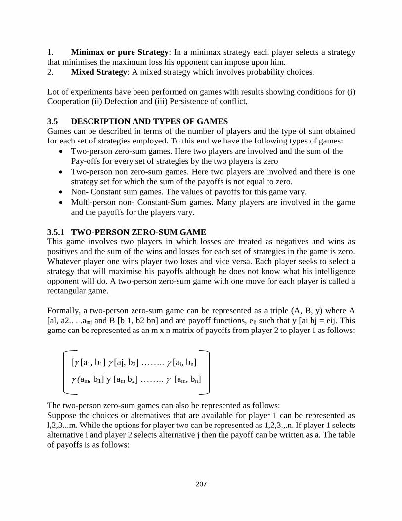
207

1. Minimax or pure Strategy: In a minimax strategy each player selects a strategy

that minimises the maximum loss his opponent can impose upon him.

2. Mixed Strategy: A mixed strategy which involves probability choices.

Lot of experiments have been performed on games with results showing conditions for (i)

Cooperation (ii) Defection and (iii) Persistence of conflict,

3.5 DESCRIPTION AND TYPES OF GAMES Games can be described in terms of the number of players and the type of sum obtained

for each set of strategies employed. To this end we have the following types of games:

Two-person zero-sum games. Here two players are involved and the sum of the

Pay-offs for every set of strategies by the two players is zero

Two-person non zero-sum games. Here two players are involved and there is one

strategy set for which the sum of the payoffs is not equal to zero.

Non- Constant sum games. The values of payoffs for this game vary.

Multi-person non- Constant-Sum games. Many players are involved in the game

and the payoffs for the players vary.

3.5.1 TWO-PERSON ZERO-SUM GAME This game involves two players in which losses are treated as negatives and wins as

positives and the sum of the wins and losses for each set of strategies in the game is zero.

Whatever player one wins player two loses and vice versa. Each player seeks to select a

strategy that will maximise his payoffs although he does not know what his intelligence

opponent will do. A two-person zero-sum game with one move for each player is called a

rectangular game.

Formally, a two-person zero-sum game can be represented as a triple (A, B, y) where A

[al, a2.. . .amj and B [b 1, b2 bn] and are payoff functions, eij such that y [ai bj = eij. This

game can be represented as an m x n matrix of payoffs from player 2 to player 1 as follows:

[ [a1, b1] [aj, b2] …….. [ai, bn]

(am, b1] y [am b2] …….. [am, bn]

The two-person zero-sum games can also be represented as follows:

Suppose the choices or alternatives that are available for player 1 can be represented as

l,2,3...m. While the options for player two can be represented as 1,2,3.,.n. If player 1 selects

alternative i and player 2 selects alternative j then the payoff can be written as a. The table

of payoffs is as follows:

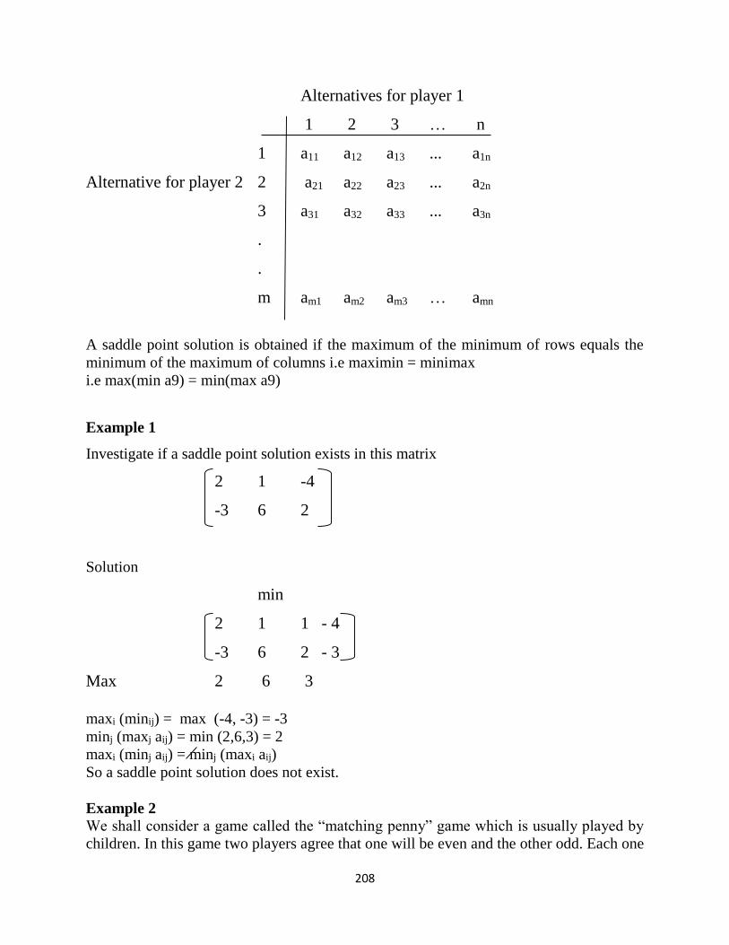
208

Alternatives for player 1

1 2 3 … n

1 a11 a12 a13 ... a1n

Alternative for player 2 2 a21 a22 a23 ... a2n

3 a31 a32 a33 ... a3n

.

.

m am1 am2 am3 … amn

A saddle point solution is obtained if the maximum of the minimum of rows equals the

minimum of the maximum of columns i.e maximin = minimax

i.e max(min a9) = min(max a9)

Example 1

Investigate if a saddle point solution exists in this matrix

2 1 -4

-3 6 2

Solution

min

2 1 1 - 4

-3 6 2 - 3

Max 2 6 3

maxi (minij) = max (-4, -3) = -3

minj (maxj aij) = min (2,6,3) = 2

maxi (minj aij) = minj (maxi aij)

So a saddle point solution does not exist.

Example 2

We shall consider a game called the “matching penny” game which is usually played by

children. In this game two players agree that one will be even and the other odd. Each one

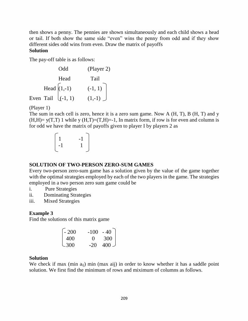
209

then shows a penny. The pennies are shown simultaneously and each child shows a head

or tail. If both show the same side “even” wins the penny from odd and if they show

different sides odd wins from even. Draw the matrix of payoffs

Solution

The pay-off table is as follows:

Odd (Player 2)

Head Tail

Head (1,-1) (-1, 1)

Even Tail (-1, 1) (1,-1)

(Player 1)

The sum in each cell is zero, hence it is a zero sum game. Now A (H, T), B (H, T) and y

(H,H)= y(T,T) 1 while y (H,T)=(T,H)=-1, In matrix form, if row is for even and column is

for odd we have the matrix of payoffs given to player I by players 2 as

1 -1

-1 1

SOLUTION OF TWO-PERSON ZERO-SUM GAMES

Every two-person zero-sum game has a solution given by the value of the game together

with the optimal strategies employed by each of the two players in the game. The strategies

employed in a two person zero sum game could be

i. Pure Strategies

ii. Dominating Strategies

iii. Mixed Strategies

Example 3

Find the solutions of this matrix game

- 200 -100 - 40

400 0 300

300 -20 400

Solution

We check if max (min aij) min (max aij) in order to know whether it has a saddle point

solution. We first find the minimum of rows and miximum of columns as follows.

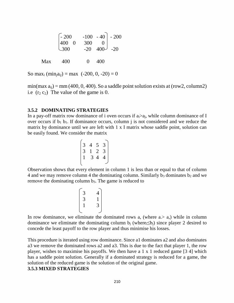
210

- 200 -100 - 40 - 200

400 0 300 0

300 -20 400 -20

Max 400 0 400

So maxi (minjaij) = max (-200, 0, -20) = 0

min(max aij) = mm (400, 0, 400). So a saddle point solution exists at (row2, column2)

i.e (r2 c2) The value of the game is 0.

3.5.2 DOMINATING STRATEGIES

In a pay-off matrix row dominance of i oven occurs if ai>aj, while column dominance of I

over occurs if b1 b1. If dominance occurs, column j is not considered and we reduce the

matrix by dominance until we are left with 1 x I matrix whose saddle point, solution can

be easily found. We consider the matrix

3 4 5 3

3 1 2 3

1 3 4 4

Observation shows that every element in column 1 is less than or equal to that of column

4 and we may remove column 4 the dominating column. Similarly b3 dominates b2 and we

remove the dominating column b3. The game is reduced to

3 4

3 1

1 3

In row dominance, we eliminate the dominated rows a, (where a.> a,) while in column

dominance we eliminate the dominating column bj (wherei≤bj) since player 2 desired to

concede the least payoff to the row player and thus minimise his losses.

This procedure is iterated using row dominance. Since a1 dominates a2 and also dominates

a3 we remove the dominated rows a2 and a3. This is due to the fact that player 1, the row

player, wishes to maximise his payoffs. We then have a 1 x 1 reduced game [3 4] which

has a saddle point solution. Generally if a dominated strategy is reduced for a game, the

solution of the reduced game is the solution of the original game.

3.5.3 MIXED STRATEGIES

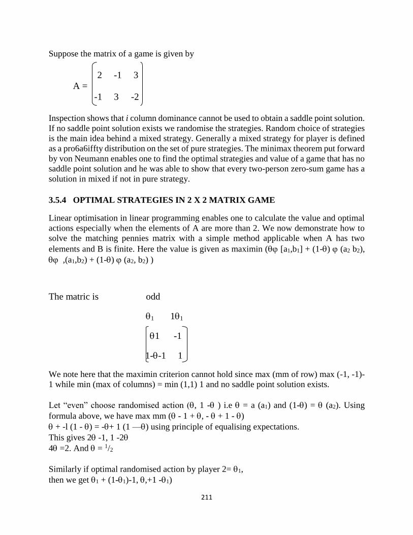
211

Suppose the matrix of a game is given by

2 -1 3

A =

-1 3 -2

Inspection shows that i column dominance cannot be used to obtain a saddle point solution.

If no saddle point solution exists we randomise the strategies. Random choice of strategies

is the main idea behind a mixed strategy. Generally a mixed strategy for player is defined

as a pro6a6iffty distribution on the set of pure strategies. The minimax theorem put forward

by von Neumann enables one to find the optimal strategies and value of a game that has no

saddle point solution and he was able to show that every two-person zero-sum game has a

solution in mixed if not in pure strategy.

3.5.4 OPTIMAL STRATEGIES IN 2 X 2 MATRIX GAME

Linear optimisation in linear programming enables one to calculate the value and optimal

actions especially when the elements of A are more than 2. We now demonstrate how to

solve the matching pennies matrix with a simple method applicable when A has two

elements and B is finite. Here the value is given as maximin ( [a1,b1] + (1-) (a2 b2),

,(a1,b2) + (1-) (a2, b2) )

The matric is odd

1 11

1 -1

1--1 1

We note here that the maximin criterion cannot hold since max (mm of row) max (-1, -1)-

1 while min (max of columns) = min (1,1) 1 and no saddle point solution exists.

Let “even” choose randomised action (, 1 - ) i.e = a (a1) and (1-) = (a2). Using

formula above, we have max mm ( - 1 + , - + 1 - )

+ -l (1 - ) = -+ 1 (1 —) using principle of equalising expectations.

This gives 2 -1, 1 -2

4 =2. And = 1/2

Similarly if optimal randomised action by player 2= 1,

then we get 1 + (1-1)-1, ,+1 -1)

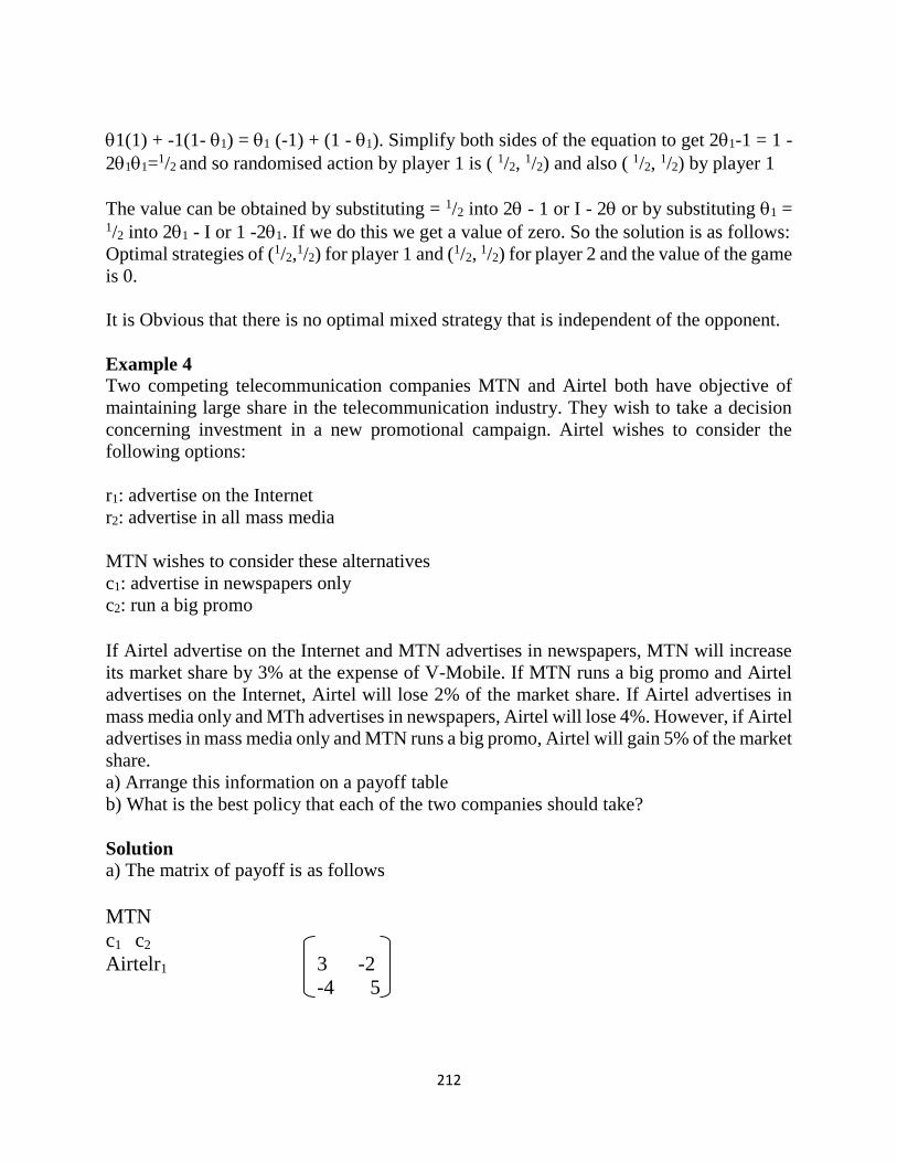
212

1(1) + -1(1- 1) = 1 (-1) + (1 - 1). Simplify both sides of the equation to get 21-1 = 1 -

211=1/2 and so randomised action by player 1 is ( 1/2, 1/2) and also ( 1/2, 1/2) by player 1

The value can be obtained by substituting = 1/2 into 2 - 1 or I - 2 or by substituting 1 = 1/2 into 21 - I or 1 -21. If we do this we get a value of zero. So the solution is as follows:

Optimal strategies of (1/2,1/2) for player 1 and (1/2, 1/2) for player 2 and the value of the game

is 0.

It is Obvious that there is no optimal mixed strategy that is independent of the opponent.

Example 4

Two competing telecommunication companies MTN and Airtel both have objective of

maintaining large share in the telecommunication industry. They wish to take a decision

concerning investment in a new promotional campaign. Airtel wishes to consider the

following options:

r1: advertise on the Internet

r2: advertise in all mass media

MTN wishes to consider these alternatives

c1: advertise in newspapers only

c2: run a big promo

If Airtel advertise on the Internet and MTN advertises in newspapers, MTN will increase

its market share by 3% at the expense of V-Mobile. If MTN runs a big promo and Airtel

advertises on the Internet, Airtel will lose 2% of the market share. If Airtel advertises in

mass media only and MTh advertises in newspapers, Airtel will lose 4%. However, if Airtel

advertises in mass media only and MTN runs a big promo, Airtel will gain 5% of the market

share.

a) Arrange this information on a payoff table

b) What is the best policy that each of the two companies should take?

Solution

a) The matrix of payoff is as follows

MTN

c1 c2

Airtelr1 3 -2

-4 5

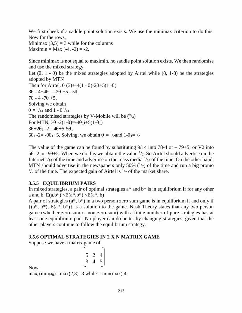
213

We first cheek if a saddle point solution exists. We use the minimax criterion to do this.

Now for the rows,

Minimax (3,5) = 3 while for the columns

Maximin = Max (-4, -2) = -2.

Since minimax is not equal to maximin, no saddle point solution exists. We then randomise

and use the mixed strategy.

Let (, 1 - ) be the mixed strategies adopted by Airtel while (8, 1-8) be the strategies

adopted by MTN

Then for Airtel. (3)+-4(1 - )-2+5(1 -)

3 - 4+4 =-2 +5 - 5

7 - 4 -7 +5.

Solving we obtain

= 9/14 and 1 - 5/14

The randomised strategies by V-Mobile will be (9/4)

For MTN, 3 -2(1-)=-41i+5(1-1)

3+21 - 2=-4+5-51

51 -2= -91+5. Solving, we obtain 1= 1/2and 1-1=1/2

The value of the game can be found by substituting 9/14 into 78-4 or – 79+5; or V2 into

5 -2 or -9+5. When we do this we obtain the value 1/2. So Airtel should advertise on the

Internet 9/14 of the time and advertise on the mass media 5/14 of the time. On the other hand,

MTN should advertise in the newspapers only 50% (1/2) of the time and run a big promo 1/2 of the time. The expected gain of Airtel is 1/2 of the market share.

3.5.5 EQUILIBRIUM PAIRS

In mixed strategies, a pair of optimal strategies a* and b* is in equilibrium if for any other

a and b, E(a,b*) <E(a*,b*) <E(a*, b)

A pair of strategies (a*, b*) in a two person zero sum game is in equilibrium if and only if

{(a*, b*), E(a*, b*)} is a solution to the game. Nash Theory states that any two person

game (whether zero-sum or non-zero-sum) with a finite number of pure strategies has at

least one equilibrium pair. No player can do better by changing strategies, given that the

other players continue to follow the equilibrium strategy.

3.5.6 OPTIMAL STRATEGIES IN 2 X N MATRIX GAME

Suppose we have a matrix game of

5 2 4

3 4 5 Now

maxi (minjaij)= max(2,3)=3 while = min(max) 4.

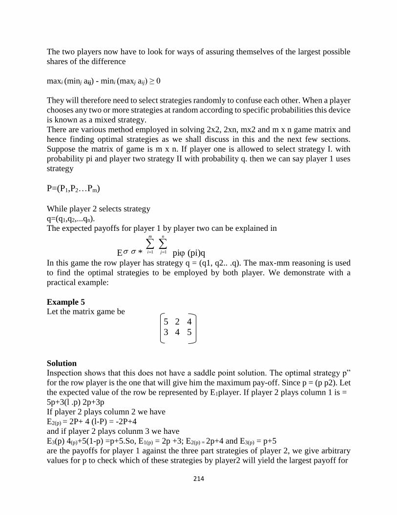
214

The two players now have to look for ways of assuring themselves of the largest possible

shares of the difference

maxi (minj aij) - mini (maxj aij) ≥ 0

They will therefore need to select strategies randomly to confuse each other. When a player

chooses any two or more strategies at random according to specific probabilities this device

is known as a mixed strategy.

There are various method employed in solving 2x2, 2xn, mx2 and m x n game matrix and

hence finding optimal strategies as we shall discuss in this and the next few sections.

Suppose the matrix of game is m x n. If player one is allowed to select strategy I. with

probability pi and player two strategy II with probability q. then we can say player 1 uses

strategy

P=(P1,P2…Pm)

While player 2 selects strategy

q=(q1,q2,...qn).

The expected payoffs for player 1 by player two can be explained in

E *

n

j

m

i 11 pi (pi)q In this game the row player has strategy q = (q1, q2.. .q). The max-mm reasoning is used

to find the optimal strategies to be employed by both player. We demonstrate with a

practical example:

Example 5

Let the matrix game be

5 2 4

3 4 5

Solution

Inspection shows that this does not have a saddle point solution. The optimal strategy p”

for the row player is the one that will give him the maximum pay-off. Since p = (p p2). Let

the expected value of the row be represented by E1player. If player 2 plays column 1 is =

5p+3(l .p) 2p+3p

If player 2 plays column 2 we have

E2(p) = 2P+ 4 (l-P) = -2P+4

and if player 2 plays colunm 3 we have

E3(p) 4(p)+5(1-p) =p+5.So, E1(p) = 2p +3; E2(p) = 2p+4 and E3(p) = p+5

are the payoffs for player 1 against the three part strategies of player 2, we give arbitrary

values for p to check which of these strategies by player2 will yield the largest payoff for

215

player 1.

Let p 3/4 ……. E1=-2x3/4+3=41/2

E2(p) = 2x¼+421/2 E2(p) =-3/4+5=41/4.

So the two largest are E1(p), E3(p) and we equate them to get

2p = 3 = p+5

so 3p= 2, p=2/3

Ej(p) = (2 x 2/3) + 3 41/3

E = -2(p) -2 x 22/3 + 4 = 22/3 and E3(p) = 2/3 + 5 = 741/3

So(2/3, 1/3) is optimal for player 1. To get the optimal strategy for player 2, we observe that

it is advisable for player 2 to play column 2 in other to ensure that the payoff to row player

is minimal. So the game is reduced to

5 4

3 5

Let (q, l-q) be the strategy for player 2 in a required game.

So 5q + 4 (1-q) 3q +5(l-q)

5q+4-4q=3q+5-5q

q +45-2q

3q=l q=1/3

So it is optimal for player 2 to play mixed strategy with probability q(1/3,O,2/3).If we

substitute q = 1/3 into q+4 or 5-2q, we obtain 41/3 as before. This is the value of the game.

4.0 CONCLUSION






of all the parties.

5.0 SUMMARY

Making decision is an integral and continuous aspect of human life. For child or adult, man

or woman, government official or business executive, worker or supervisor, participation

in the process of decision- making is a common feature of everyday life. A competitive

situation is called a game if it has the following characteristics- there is finite number of

competitors called Players. A list of finite or infinite number of possible courses of action

is available to each player; a list of finite or infinite number of possible courses of action

is available to each player; a play is played when each player chooses one of his courses of

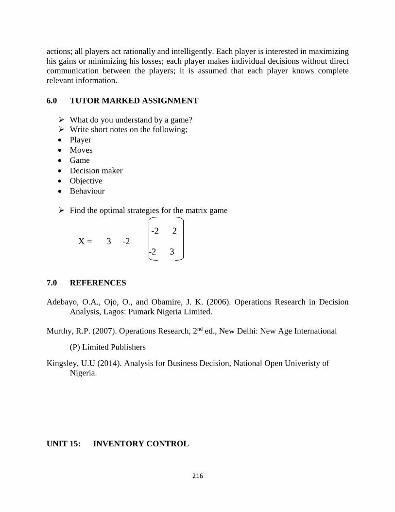
216

actions; all players act rationally and intelligently. Each player is interested in maximizing

his gains or minimizing his losses; each player makes individual decisions without direct

communication between the players; it is assumed that each player knows complete

relevant information.


What do you understand by a game?

Write short notes on the following;

Player

Moves

Game

Decision maker

Objective

Behaviour

Find the optimal strategies for the matrix game

-2 2

X = 3 -2

-2 3

7.0 REFERENCES

Adebayo, O.A., Ojo, O., and Obamire, J. K. (2006). Operations Research in Decision


Murthy, R.P. (2007). Operations Research, 2nd ed., New Delhi: New Age International

(P) Limited Publishers


Nigeria.

UNIT 15: INVENTORY CONTROL

217

1.0 Introduction

2.0 Objective

3.0 Main Content

3.1 Definition of Inventory and Inventory Control

3.2 Basic Concepts in Inventory Planning

3.3 Necessity for Maintaining Inventory

3.4 Causes of Poor Inventory Control Systems

3.5 Classification of Inventories

3.6 Costs Associated With Inventory

3.7 Purpose of Maintaining Inventory or Objective of Inventory cost Control

3.8 Other Factors to be considered in Inventory Control

3.9 Inventory Control Problem

3.10 The Classical EOQ Model (Demand Rate Uniform, Replenishment Rate

Infinite)

4.0 Conclusion

5.0 Summary


7.0 References

1.0 INTRODUCTION

One of the basic functions of management is to employ capital efficiently so as to yield the

maximum returns. This can be done in either of two ways or by both, i.e. (a) By maximizing

the margin of profit; or (b) By maximizing the production with a given amount of capital,

i.e. to increase the productivity of capital. This means that the management should try to

make its capital work hard as possible. However, this is all too often neglected and much

time and ingenuity are devoted to make only labour work harder. In the process, the capital

turnover and hence the productivity of capital is often totally neglected.







improving their productivity.

2.0 OBJECTIVES

At the this study unit, you should be able to

Define inventory control

Explain the basic concepts in inventory control

Identify the issues that necessitate maintaining inventory

Identify causes of poor inventory control systems

Discuss the various classifications of inventories

218

3.0 MAIN CONTENT

3.1 DEFINITION OF INVENTORY AND INVENTORY CONTROL

The word inventory means a physical stock of material or goods or commodities or other

economic resources that are stored or reserved or kept in stock or in hand for smooth and

efficient running of future affairs of an organization at the minimum cost of funds or capital

blocked in the form of materials or goods (Inventories). The function of directing the

movement of goods through the entire manufacturing cycle from the requisitioning of raw

materials to the inventory of finished goods in an orderly manner to meet the objectives of

maximum customer service with minimum investment and efficient (low cost) plant

operation is termed as inventory control. (Murthy, 2007)

Gupta and Hira (2012) defined an inventory as consisting of usable but idle resources such


inventory is called stock. An inventory problem is said to exist if either the resources are

subject to control or if there is at least one such cost that decrease as inventory increases.

The objective is to minimise total (actual or expected) cost. However, in situations where

inventory affects demand, the objective may also be to minimise profit.

3.2 BASIC CONCEPTS IN INVENTORY PLANNING

For many organizations, inventories represent a major capital cost, in some cases the

dominant cost, so that the management of this capital becomes of the utmost importance.

When considering the inventories, we need to distinguish different classes of items that are

kept in stock. In practice, it turns out that about 10% of the items that are kept in stock

usually account for something in the order of 60% of the value of all inventories. Such

items are therefore of prime concern to the company, and the stock of these items will need

close attention. These most important items are usually referred to as “A items” in the ABC

classification system developed by the General Electric Company in the 1950s. The items

next in line are the B items, which are of intermediate importance. They typically represent

30% of the items, corresponding to about 30% of the total inventory value. Clearly, B items

do require some attention, but obviously less than A items. Finally, the bottom 60% of the

items are the C items. They usually represent maybe 10% of the monetary value of the total

inventory. The control of C items in inventory planning is less crucial than that of the A

and B items. The models in this chapter are mostly aimed at A items.

3.3 NECESSITY FOR MAINTAINING INVENTORY

Though inventory of materials is an idle resource (since materials lie idle and are not to be

used immediately), almost every organisation. Without it, no business activity can be

performed, whether it is service organisation like a hospital or a bank or it a manufacturing

or trading organisation. Gupta and Hira (2012) present the following reasons for maintain

inventories in organisations.

6. It helps in the smooth and efficient of an enterprise.

219

7. It helps in providing service to the customer at short notice.

8. In the absence of inventory, the enterprise may have to pay high prices due to

piecemeal purchasing.

9. It reduces product cost since there is an added advantage of batching and long,

uninterrupted production runs.

10. It acts as a buffer stock when raw materials are received late and shop rejection is

too many.

3.4 CAUSES OF POOR INVENTORY CONTROL SYSTEMS

e. Overbuying without regard to the forecast or proper estimate of demand to take

advantages of favourable market.

f. Overproduction or production of goods much before the customer requires them

g. Overstocking may also result from the desire to provide better service to the custom.

h. Cancellation of orders and minimum quantity stipulations by the suppliers may also

give rise to large inventories.


3.5 CLASSIFICATION OF INVENTORIES

Inventories may be classified as those which play direct role during manufacture or which

can be identified on the product and the second one are those which are required for

manufacturing but not as a part of production or cannot be identified on the product. The

first type is labelled as direct inventories and the second are labelled as indirect

inventories. Further classification of direct and indirect inventories is as follows:

A. Direct inventories

(i) Raw material inventories or Production Inventories: The inventory of raw materials

is the materials used in the manufacture of product and can be identified on the product. In

inventory control manager can concentrate on the

(a) Bulk purchase of materials to save the investment,

(b) To meet the changes in production rate,

(c) To plan for buffer stock or safety stock to serve against the delay in delivery of

inventory against orders placed and also against seasonal fluctuations. Direct inventories

include the following:

Production Inventories- items such as raw materials, components and

subassemblies used to produce the final products.

Work-in-progress Inventory- items in semi-finished form or products at different

stages of production.

Miscellaneous Inventory- all other items such as scrap, obsolete and unsaleable

products, stationary and other items used in office, factory and sales department,

etc.

(ii) Work-in -process inventories or in process inventories: These inventories are of semi-

finished type, which are accumulated between operations or facilities.As far as possible,

holding of materials between operations to be minimized if not avoided. This is because;

220

as we process the materials the economic value (added labour cost) and use value are added

to the raw material, which is drawn from stores. Hence if we hold these semi-finished

material for a

long time the inventory carrying cost goes on increasing, which is not advisable in

inventory control. These inventories serve the following purposes:

(a) Provide economical lot production,

(b) Cater to the variety of products,

(c) Replacement of wastages,

(d) To maintain uniform production even if sales varies.

(iii) Finished goods inventories: After finishing the production process and packing, the

finished products are stocked in stock room. These are known as finished goods inventory.

These are maintained to:

(a) To ensure the adequate supply to the customers,

(b) To allow stabilization of the production level and

(c) To help sales promotion programme.

(iv) MRO Inventory or Spare parts inventories: Maintenance, Repair, and Operation items

such as spare parts and consumable stores that do not go into final products but are

consumed during the production process. Any product sold to the customer, will be

subjected to wear and tear due to usage and the customer has to replace the worn-out part.

Hence the manufacturers always calculate the life of the various components of his product

and try to supply the spare components to the market to help after sales service. The use of

such spare parts inventory is:

(a) To provide after sales service to the customer,

(b) To utilize the product fully and economically by the customer.

(iv) Scrap or waste inventory or Miscellaneous Inventory: While processing the materials,

we may come across certain wastages and certain bad components (scrap), which are of no

use. These may be used by some other industries as raw material. These are to be collected

and kept in a place away from main stores and are disposed periodically by auctioning.

B. Indirect Inventories

Inventories or materials like oils, grease, lubricants, cotton waste and such other materials

are required during the production process. But we cannot identify them on the product.

These are known as indirect inventories. In our discussion of inventories, in this chapter,

we only discuss about the direct inventories. Inventories may also be classified depending

on their nature of use. They are:

(i) Fluctuation Inventories: These inventories are carried out to safeguard the fluctuation

in demand, non-delivery of material in time due to extended lead-time. These are

sometimes called as Safety stock or reserves. In real world inventory situations, the

material may not be received in time as expected due to trouble in transport system or some

221

times, the demand for a certain material may increase unexpectedly. To safeguard such

situations, safety stocks are maintained. The level of this stock will fluctuate depending on

the demand and lead-time etc.

(ii) Anticipation inventory: When there is an indication that the demand for company’s

product is going to be increased in the coming season, a large stock of material is stored in

anticipation. Some times in anticipation of raising prices, the material is stocked. Such

inventories, which are stocked in anticipation of raising demand or raising rises, are known

as anticipation inventories.

(iii) Lot size inventory or Cycle inventories: This situation happens in batch production

system. In this system products are produced in economic batch quantities. It sometime

happens that the materials are procured in quantities larger than the economic quantities to

meet the fluctuation in demand. In such cases the excess materials are stocked, which are

known as lot size or cycle inventories.

3.6 COSTS ASSOCIATED WITH INVENTORY

While maintaining the inventories, we will come across certain costs associated with

inventory, which are known as economic parameters. Most important of them are

discussed below:

A. Inventory Carrying Charges, or Inventory Carrying Cost or Holding Cost or

Storage Cost (C1) or (i%)

This cost arises due to holding of stock of material in stock. This cost includes the cost of

maintaining the inventory and is proportional to the quantity of material held in stock and

the time for which the material is maintained in stock. The components of inventory

carrying cost are:

i. Rent for the building in which the stock is maintained if it is a rented building. In case it

is own building, depreciation cost of the building is taken into consideration. Sometimes

for own buildings, the nominal rent is calculated depending on the local rate of rent and is

taken into consideration.

ii. It includes the cost of equipment if any and cost of racks and any special facilities used

in the stores.

iii. Interest on the money locked in the form of inventory or on the money invested in

purchasing the inventory.

iv. The cost of stationery used for maintaining the inventory.

v. The wages of personnel working in the stores.

vi. Cost of depreciation, insurance.

B. Shortage cost or Stock - out - cost- (C2)

222

Sometimes it so happens that the material may not be available when needed or when the

demand arises. In such cases the production has to be stopped until the procurement of the

material, which may lead to miss the delivery dates or delayed production. When the

organization could not meet the delivery promises, it has to pay penalty to the customer. If

the situation of stock out will occur very often, then the customer may not come to the

organization to place orders that is the organization is losing the customers In other words,

the organization is losing the goodwill of the customers The cost of good will cannot be

estimated. In some cases it will be very heavy to such extent that the organization has to

forego its business. Here to avoid the stock out situation, if the organization stocks more

material, inventory carrying cost increases and to take care of inventory cost, if the

organization purchases just sufficient or less quantity, then the stock out position may arise.

Hence the inventory manager must have sound knowledge of various factors that are

related to inventory carrying cost andstock out cost and estimate the quantity of material

to be purchased or else he must have effective strategies to face grave situations. The cost

is generally represented as so many naira and is represented by C2.

C. Set up cost or Ordering cost or Replenishment Cost (C3)

For purchase models, the cost is termed as ordering cost or procurement cost and for

manufacturing cost it is termed as set up cost and is represented by C3.

(i) Set up cost: The term set up cost is used for production or manufacturing models.

Whenever a job is to be produced, the machine is to set to produce the job. That is the tool

is to be set and the material is to be fixed in the jobholder. This consumes some time.

During this time the machine will be idle and the labour is working. The cost of idle

machine and cost of labour charges are to be added to the cost of production. If we produce

only one job in one set up, the entire set up cost is to be charged to one job only. In case

we produce ‘n’ number of jobs in one set up, the set up cost is shared by ‘n’ jobs. In case

of certain machines like N.C machines, or Jig boarding machine, the set up time may be

15 to 20 hours. The idle cost of the machine and labour charges may work out to few

thousands of naira. Once the machine set up is over, the entire production can be completed

in few hours if we produce more number of products in one set up the set up cost is allocated

to all the jobs equally. This

reduces the production cost of the product. For example let us assume that the set up cost

is N 1000/-. If we produce 10 jobs in one set up, each job is charged with N 100/- towards

the set up cost. In case, if we produce 100 jobs, the set up cost per job will be N10/-. If we

produce, 1000 jobs in one set up, the set up cost per job will be Re. 1/- only. This can be

shown by means of a graph as shown in figure 15.1.

(ii) Ordering Cost or Replenishment Cost: The term Ordering cost or Replenishment cost

is used in purchase models. Whenever any material is to be procured by an organization, it

has to place an order with the supplier. The cost of stationary used for placing the order,

the cost of salary of officials involved in preparing the order and the postal expenses and

after placing the order enquiry charges all put together, is known as ordering cost. In Small

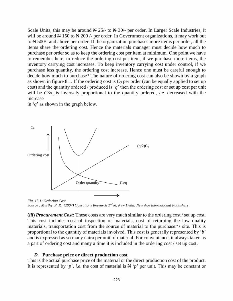
223

Scale Units, this may be around N 25/- to N 30/- per order. In Larger Scale Industries, it

will be around N 150 to N 200 /- per order. In Government organizations, it may work out

to N 500/- and above per order. If the organization purchases more items per order, all the

items share the ordering cost. Hence the materials manager must decide how much to

purchase per order so as to keep the ordering cost per item at minimum. One point we have

to remember here, to reduce the ordering cost per item, if we purchase more items, the

inventory carrying cost increases. To keep inventory carrying cost under control, if we

purchase less quantity, the ordering cost increase. Hence one must be careful enough to

decide how much to purchase? The nature of ordering cost can also be shown by a graph

as shown in figure 8.1. If the ordering cost is C3 per order (can be equally applied to set up

cost) and the quantity ordered / produced is ‘q’ then the ordering cost or set up cost per unit

will be C3/q is inversely proportional to the quantity ordered, i.e. decreased with the

increase

in ‘q’ as shown in the graph below.

C0

(q/2)C1

Ordering cost

Order quantity C3/q

Fig. 15.1: Ordering Cost

Source : Murthy, P. R. (2007) Operations Research 2nded. New Delhi: New Age International Publishers

(iii) Procurement Cost: These costs are very much similar to the ordering cost / set up cost.

This cost includes cost of inspection of materials, cost of returning the low quality

materials, transportation cost from the source of material to the purchaser‘s site. This is

proportional to the quantity of materials involved. This cost is generally represented by ‘b’

and is expressed as so many naira per unit of material. For convenience, it always taken as

a part of ordering cost and many a time it is included in the ordering cost / set up cost.

D. Purchase price or direct production cost

This is the actual purchase price of the material or the direct production cost of the product.

It is represented by ‘p’. i.e. the cost of material is N ‘p’ per unit. This may be constant or

224

variable. Say for example the cost of an item is N 10/- item if we purchase 1 to 10 units. In

case we purchase more than 10 units, 10 percent discount is allowed. i.e. the cost of item

will be N9/- per unit. The purchase manager can take advantage of discount allowed by

purchasing more. But this will increase the inventory carrying charges. As we are

purchasing more per order, ordering cost is reduced and because of discount, material cost

is reduced. Materials manager has to take into consideration these cost – quantity

relationship and decide how much to purchase to keep the inventory cost at low level.

3.7 PURPOSE OF MAINTAINING INVENTORY OR OBJECTIVE OF

INVENTORY COST CONTROL

The purpose of maintaining the inventory or controlling the cost of inventory is to use the

available capital optimally (efficiently) so that inventory cost per item of material will be

as small as possible. For this the materials manager has to strike a balance between the

interrelated inventory costs. In the process of balancing the interrelated costs i.e. Inventory

carrying cost, ordering cost or set up cost, stock out cost and the actual material cost. Hence

we can say that the objective of controlling the inventories is to enable the materials

manager to place and order at right time with the right source at right price to purchase

right quantity. The benefits derived from efficient inventory control are:

i. It ensures adequate supply of goods to the customer or adequate of quantity of raw

materials to the manufacturing department so that the situation of stock out may be reduced

or avoided.

ii. By proper inventory cost control, the available capital may be used efficiently or

optimally, by avoiding the unnecessary expenditure on inventory.

iii. In production models, while estimating the cost of the product the material cost is to be

added. The manager has to decide whether he has to take the actual purchase price of the

material or the current market price of the material. The current market price may be less

than or greater than the purchase price of the material which has been purchased some

period back. Proper inventory control reduces such risks.

iv. It ensures smooth and efficient running of an organization and provides safety against

late delivery times to the customer due to uncontrollable factors

v. A careful materials manager may take advantage of price discounts and make bulk

purchase at the same time he can keep the inventory cost at minimum.

3.8 OTHER FACTORS TO BE CONSIDERED IN INVENTORY CONTROL

There are many factors, which have influence on the inventory, which draws the attention

of an inventory manager, they are:

(i) Demand

225

The demand for raw material or components for production or demand of goods to satisfy

the needs of the customer, can be assessed from the past consumption/supply pattern of

material or goods. We find that the demand may be deterministic in nature i.e., we can

specify that the demand for the item is so many units for example say ‘q’ units per unit of

time. Also the demand may be static, i.e. it means constant for each time period (uniform

over equal period of times).

The supply of inventory to the stock may deterministic or probabilistic (stochastic) in

nature and many a times it is uncontrollable, because, the rate of production depends on

the production, which is once again depends on so many factors which are uncontrollable

/ controllable factors Similarly supply of inventory depends on the type of supplier, mode

of supply, mode of transformation etc.

(iii) Lead time or Delivery Lags or Procurement time

Lead-time is the time between placing the order and receipt of material to the stock. In

production models, it is the time between the decisions made to take up the order and

starting of production. This time in purchase models depends on many uncontrollable

factors like transport mode, transport route, agitations etc. It may vary from few days to

few months depending on the nature of delay.

(iv) Type of goods

The inventory items may be discrete or continuous. Sometimes the discrete items are to be

considered as continuous items for the sake of convenience.

(v) Time horizon

The time period for which the optimal policy is to be formulated or the inventory cost is to

be optimized is generally termed as the Inventory planning period of Time horizon. This

time is represented on X - axis while drawing graphs. This time may be finite or infinite.

In any inventory model, we try to seek answers for the following questions:

(a) When should the inventory be purchased for replenishment? For example, the

inventory should be replenished after a period‘t’ or when the level of the inventory is qo.

(b) How much quantity must be purchased or ordered or produced at the time of

replenishment so as to minimize the inventory costs? For example, the inventory must

be purchased with the supplier who is supplying at a cost of Np/- per unit. In addition to

the above depending on the data available, we can also decide from which source we have

to purchase and what price we have to purchase? But in general time and quantity are the

two variables, we can control separately or in combination.

3.9 INVENTORY CONTROL PROBLEM

The inventory control problem consists of the determination of three basic factors:

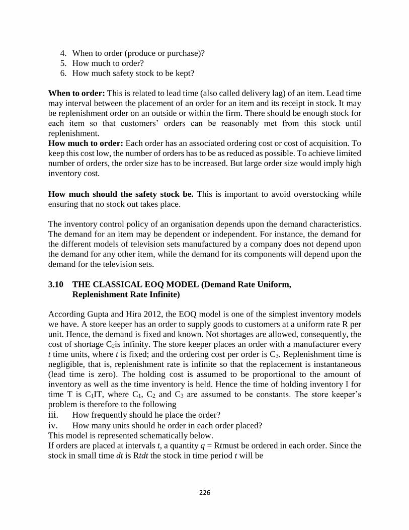
226

4. When to order (produce or purchase)?

5. How much to order?

6. How much safety stock to be kept?

When to order: This is related to lead time (also called delivery lag) of an item. Lead time

may interval between the placement of an order for an item and its receipt in stock. It may

be replenishment order on an outside or within the firm. There should be enough stock for

each item so that customers’ orders can be reasonably met from this stock until

replenishment.

How much to order: Each order has an associated ordering cost or cost of acquisition. To

keep this cost low, the number of orders has to be as reduced as possible. To achieve limited

number of orders, the order size has to be increased. But large order size would imply high

inventory cost.

How much should the safety stock be. This is important to avoid overstocking while

ensuring that no stock out takes place.

The inventory control policy of an organisation depends upon the demand characteristics.

The demand for an item may be dependent or independent. For instance, the demand for

the different models of television sets manufactured by a company does not depend upon

the demand for any other item, while the demand for its components will depend upon the

demand for the television sets.

3.10 THE CLASSICAL EOQ MODEL (Demand Rate Uniform,

Replenishment Rate Infinite)

According Gupta and Hira 2012, the EOQ model is one of the simplest inventory models

we have. A store keeper has an order to supply goods to customers at a uniform rate R per

unit. Hence, the demand is fixed and known. Not shortages are allowed, consequently, the

cost of shortage C2is infinity. The store keeper places an order with a manufacturer every

t time units, where t is fixed; and the ordering cost per order is C3. Replenishment time is

negligible, that is, replenishment rate is infinite so that the replacement is instantaneous

(lead time is zero). The holding cost is assumed to be proportional to the amount of

inventory as well as the time inventory is held. Hence the time of holding inventory I for

time T is C1IT, where C1, C2 and C3 are assumed to be constants. The store keeper’s

problem is therefore to the following

iii. How frequently should he place the order?

iv. How many units should he order in each order placed?

This model is represented schematically below.

If orders are placed at intervals t, a quantity q = Rtmust be ordered in each order. Since the

stock in small time dt is Rtdt the stock in time period t will be

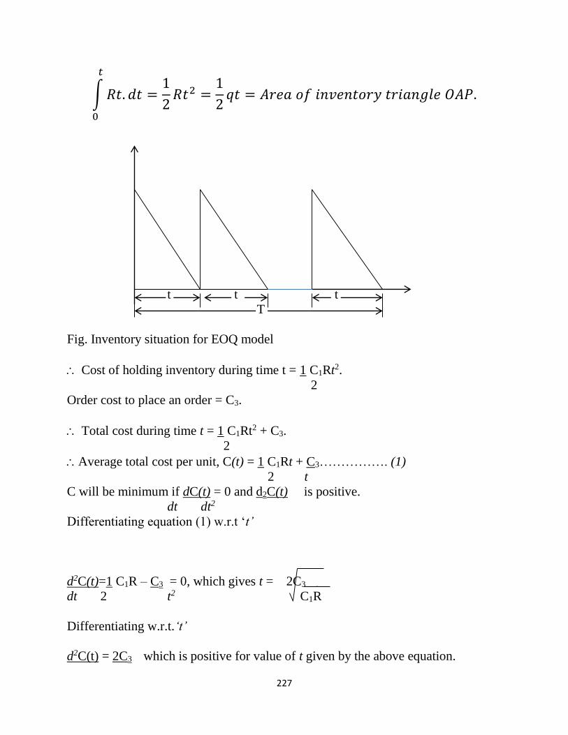
227

∫ 𝑅𝑡. 𝑑𝑡 =1

2𝑅𝑡2

𝑡

0

=1

2𝑞𝑡 = 𝐴𝑟𝑒𝑎 𝑜𝑓 𝑖𝑛𝑣𝑒𝑛𝑡𝑜𝑟𝑦 𝑡𝑟𝑖𝑎𝑛𝑔𝑙𝑒 𝑂𝐴𝑃.

t t t

T

Fig. Inventory situation for EOQ model

Cost of holding inventory during time t = 1 C1Rt2.

2

Order cost to place an order = C3.

Total cost during time t = 1 C1Rt2 + C3.

2

Average total cost per unit, C(t) = 1 C1Rt + C3……………. (1)

2 t

C will be minimum if dC(t) = 0 and d2C(t) is positive.

dt dt2

Differentiating equation (1) w.r.t ‘t’

d2C(t)=1 C1R – C3 = 0, which gives t = 2C3 .

dt 2 t2 C1R

Differentiating w.r.t.‘t’

d2C(t) = 2C3 which is positive for value of t given by the above equation.

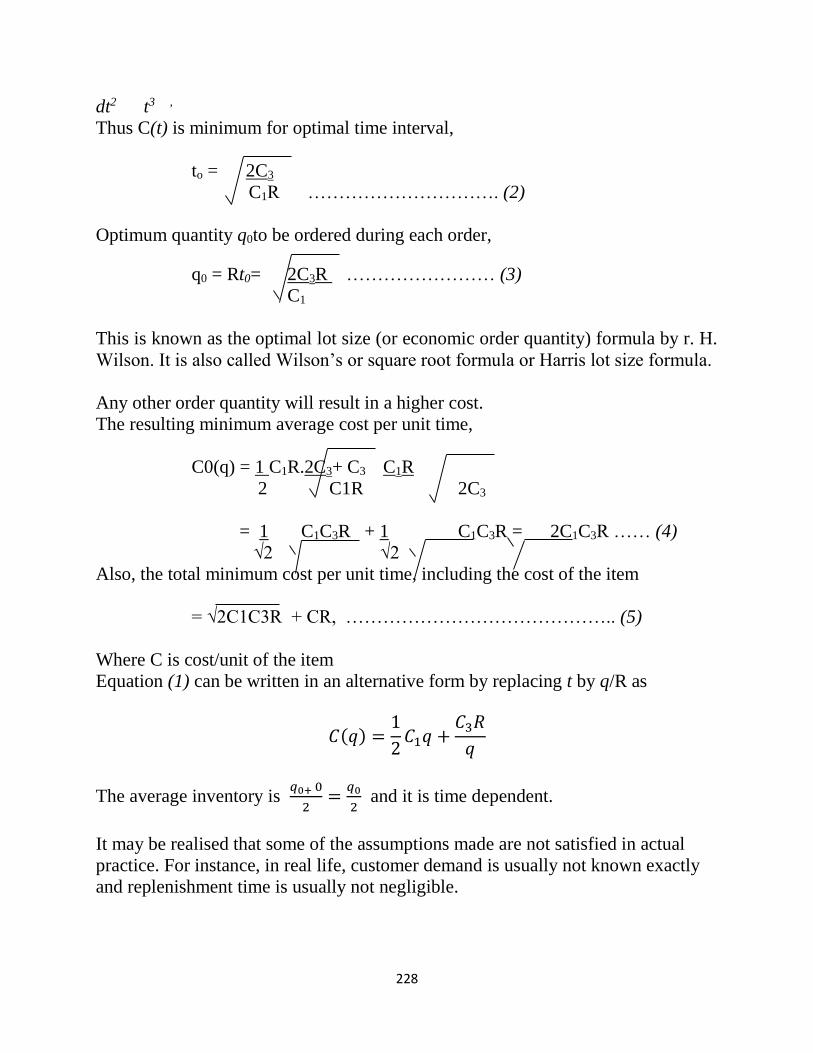
228

dt2 t3 ,

Thus C(t) is minimum for optimal time interval,

to = 2C3

C1R …………………………. (2)

Optimum quantity q0to be ordered during each order,

q0 = Rt0= 2C3R …………………… (3)

C1

This is known as the optimal lot size (or economic order quantity) formula by r. H.

Wilson. It is also called Wilson’s or square root formula or Harris lot size formula.

Any other order quantity will result in a higher cost.

The resulting minimum average cost per unit time,

C0(q) = 1 C1R.2C3+ C3 C1R

2 C1R 2C3

= 1 C1C3R + 1 C1C3R = 2C1C3R …… (4)

√2 √2

Also, the total minimum cost per unit time, including the cost of the item

= √2C1C3R + CR, …………………………………….. (5)

Where C is cost/unit of the item

Equation (1) can be written in an alternative form by replacing t by q/R as

𝐶(𝑞) =1

2𝐶1𝑞 +

𝐶3𝑅

𝑞

The average inventory is 𝑞0+ 0

2=

𝑞0

2 and it is time dependent.

It may be realised that some of the assumptions made are not satisfied in actual

practice. For instance, in real life, customer demand is usually not known exactly

and replenishment time is usually not negligible.

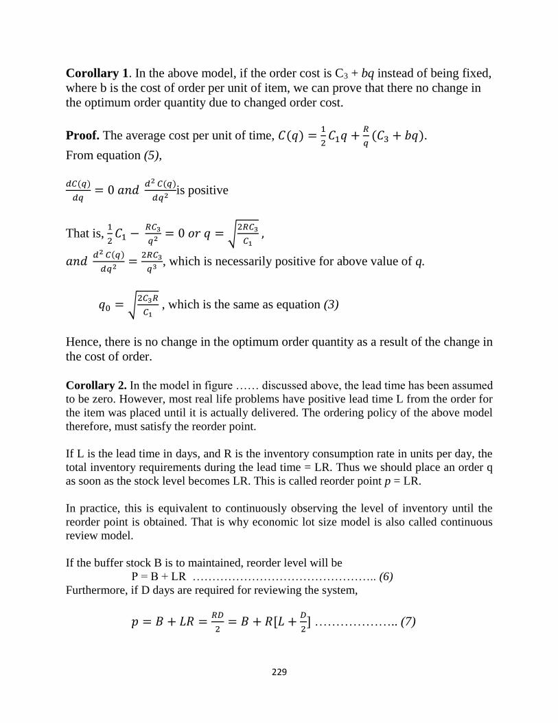
229

Corollary 1. In the above model, if the order cost is C3 + bq instead of being fixed,

where b is the cost of order per unit of item, we can prove that there no change in

the optimum order quantity due to changed order cost.

Proof. The average cost per unit of time, 𝐶(𝑞) =1

2𝐶1𝑞 +

𝑅

𝑞(𝐶3 + 𝑏𝑞).

From equation (5),

𝑑𝐶(𝑞)

𝑑𝑞= 0 𝑎𝑛𝑑

𝑑2 𝐶(𝑞)

𝑑𝑞2is positive

That is, 1

2𝐶1 −

𝑅𝐶3

𝑞2= 0 𝑜𝑟 𝑞 = √

2𝑅𝐶3

𝐶1 ,

𝑎𝑛𝑑 𝑑2 𝐶(𝑞)

𝑑𝑞2=

2𝑅𝐶3

𝑞3, which is necessarily positive for above value of q.

𝑞0 = √2𝐶3𝑅

𝐶1 , which is the same as equation (3)

Hence, there is no change in the optimum order quantity as a result of the change in

the cost of order.

Corollary 2. In the model in figure …… discussed above, the lead time has been assumed

to be zero. However, most real life problems have positive lead time L from the order for

the item was placed until it is actually delivered. The ordering policy of the above model

therefore, must satisfy the reorder point.

If L is the lead time in days, and R is the inventory consumption rate in units per day, the

total inventory requirements during the lead time = LR. Thus we should place an order q

as soon as the stock level becomes LR. This is called reorder point p = LR.

In practice, this is equivalent to continuously observing the level of inventory until the

reorder point is obtained. That is why economic lot size model is also called continuous

review model.

If the buffer stock B is to maintained, reorder level will be

P = B + LR ……………………………………….. (6)

Furthermore, if D days are required for reviewing the system,

𝑝 = 𝐵 + 𝐿𝑅 =𝑅𝐷

2= 𝐵 + 𝑅[𝐿 +

𝐷

2] ……………….. (7)

230

Assumptions in the EOQ Formula

The following assumptions have been made while deriving the EOQ formula:

9. Demand is known and uniform (constant)

10. Shortages are not permitted; as soon as the stock level becomes zero, it is

instantaneously replenished.

11. Replenishment stock is instantaneous or replenishment rate is infinite.

12. Lead time is zero. The moment the order is placed, the quantity ordered is

automatically received.

13. Inventory carrying cost and ordering cost per order remain constant over time. The

former has a linear relationship with the quantity ordered and the latter with the

number of order.

14. Cost of the item remains constant over time. There are no price- breaks or quantity

discounts.

15. The item is purchased and replenished in lots or batches.

16. The inventory system relates to a single item.

Limitations of the EOQ Model

The EOQ formula has a number of limitations. It has been highly controversial since a

number of objections have been raised regarding its validity. Some of these objections are:

7. In practice, the demand neither known with certainty nor it is uniform. If the

fluctuations are mild, the formula can be applicable but for large fluctuations, it

loses its validity. Dynamic EOQ models, instead, may have to be applied.

8. The ordering cost is difficult to measure. Also it may not be linearly related to the

number of orders as assumed in the derivation of the model. The inventory carrying

rate is still more difficult to measure and even to define precisely.

9. It is difficult to predict the demand. Present demand may be quite different from the

past history. Hardly any prediction is possible for a new product to be introduced in

the market.

10. The EOQ model assumes instantaneous replenishment of the entire quantity

ordered. The practice, the total quantity may be supplied in parts. EOQ model is not

applicable in such a situation.

11. Lead time may not be zero unless the supplier is next-door and has sufficient stock

of the item, which is rarely so.

12. Price variations, quantity discounts and shortages may further invalidate the use of

the EOQ formula.

However, the flatness of the total cost curve around the minimum is an answer to the many

objections. Even if we deviate from EOQ within reasonable limits, there is no substantial

change in cost. For example, if because of inaccuracies and errors, we have selected an

order quantity 20%more (or less) than q0the increase in total cost will be less than 20%.

EXAMPLE 1

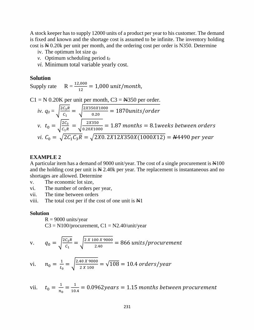
231

A stock keeper has to supply 12000 units of a product per year to his customer. The demand

is fixed and known and the shortage cost is assumed to be infinite. The inventory holding

cost is N 0.20k per unit per month, and the ordering cost per order is N350. Determine

iv. The optimum lot size q0

v. Optimum scheduling period t0

vi. Minimum total variable yearly cost.

Solution

Supply rate R = 12,000

12= 1,000 𝑢𝑛𝑖𝑡/𝑚𝑜𝑛𝑡ℎ,

C1 = N 0.20K per unit per month, C3 = N350 per order.

iv. q0 = √2𝐶3𝑅

𝐶1= √

2𝑋350𝑋1000

0.20= 1870𝑢𝑛𝑖𝑡𝑠/𝑜𝑟𝑑𝑒𝑟

v. 𝑡0 = √2𝐶3

𝐶1𝑅 = √

2𝑋350

0.20𝑋1000= 1.87 𝑚𝑜𝑛𝑡ℎ𝑠 = 8.1𝑤𝑒𝑒𝑘𝑠 𝑏𝑒𝑡𝑤𝑒𝑒𝑛 𝑜𝑟𝑑𝑒𝑟𝑠

vi. 𝐶0 = √2𝐶1𝐶3𝑅 = √2𝑋0. 2𝑋12𝑋350𝑋(1000𝑋12) = 𝑁4490 𝑝𝑒𝑟 𝑦𝑒𝑎𝑟

EXAMPLE 2

A particular item has a demand of 9000 unit/year. The cost of a single procurement is N100

and the holding cost per unit is N 2.40k per year. The replacement is instantaneous and no

shortages are allowed. Determine

v. The economic lot size,

vi. The number of orders per year,

vii. The time between orders

viii. The total cost per if the cost of one unit is N1

Solution

R = 9000 units/year

C3 = N100/procurement, C1 = N2.40/unit/year

v. 𝑞0 = √2𝐶3𝑅

𝐶1= √

2 𝑋 100 𝑋 9000

2.40= 866 𝑢𝑛𝑖𝑡𝑠/𝑝𝑟𝑜𝑐𝑢𝑟𝑒𝑚𝑒𝑛𝑡

vi. 𝑛0 = 1

𝑡0= √

2.40 𝑋 9000

2 𝑋 100= √108 = 10.4 𝑜𝑟𝑑𝑒𝑟𝑠/𝑦𝑒𝑎𝑟

vii. 𝑡0 = 1

𝑛0=

1

10.4= 0.0962𝑦𝑒𝑎𝑟𝑠 = 1.15 𝑚𝑜𝑛𝑡ℎ𝑠 𝑏𝑒𝑡𝑤𝑒𝑒𝑛 𝑝𝑟𝑜𝑐𝑢𝑟𝑒𝑚𝑒𝑛𝑡

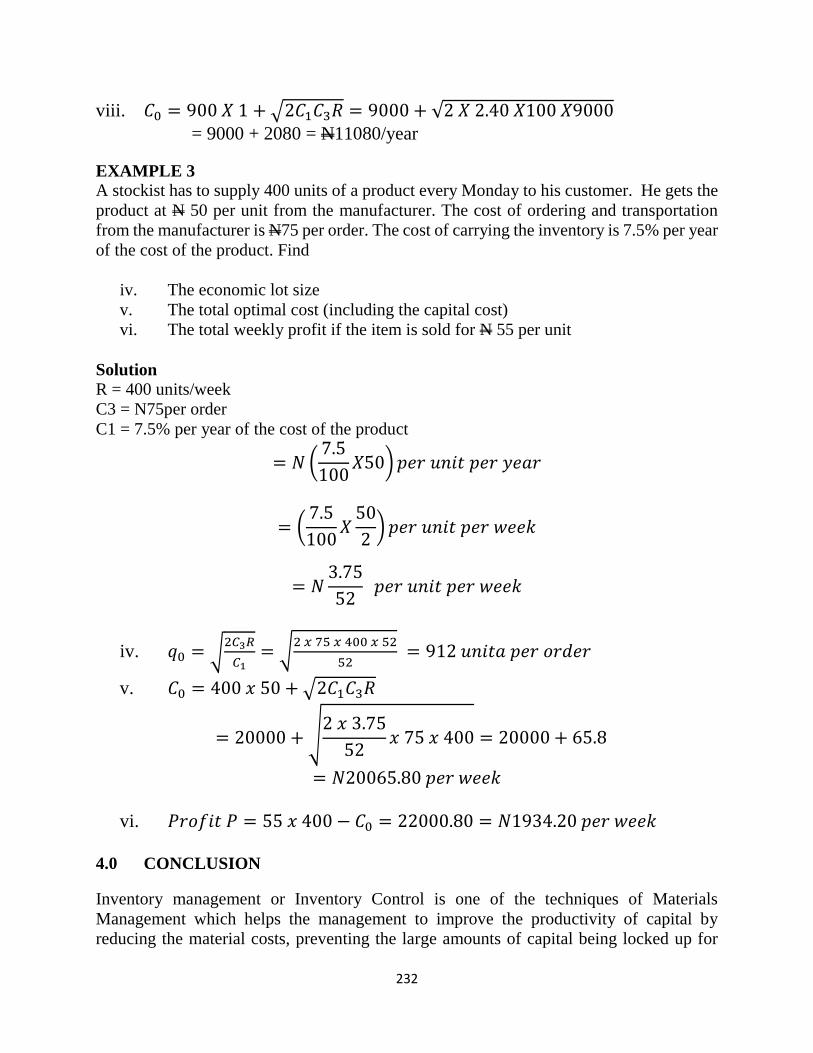
232

viii. 𝐶0 = 900 𝑋 1 + √2𝐶1𝐶3𝑅 = 9000 + √2 𝑋 2.40 𝑋100 𝑋9000

= 9000 + 2080 = N11080/year

EXAMPLE 3

A stockist has to supply 400 units of a product every Monday to his customer. He gets the

product at N 50 per unit from the manufacturer. The cost of ordering and transportation

from the manufacturer is N75 per order. The cost of carrying the inventory is 7.5% per year

of the cost of the product. Find

iv. The economic lot size

v. The total optimal cost (including the capital cost)

vi. The total weekly profit if the item is sold for N 55 per unit

Solution

R = 400 units/week

C3 = N75per order

C1 = 7.5% per year of the cost of the product

= 𝑁 (7.5

100𝑋50) 𝑝𝑒𝑟 𝑢𝑛𝑖𝑡 𝑝𝑒𝑟 𝑦𝑒𝑎𝑟

= (7.5

100𝑋

50

2) 𝑝𝑒𝑟 𝑢𝑛𝑖𝑡 𝑝𝑒𝑟 𝑤𝑒𝑒𝑘

= 𝑁3.75

52 𝑝𝑒𝑟 𝑢𝑛𝑖𝑡 𝑝𝑒𝑟 𝑤𝑒𝑒𝑘

iv. 𝑞0 = √2𝐶3𝑅

𝐶1= √

2 𝑥 75 𝑥 400 𝑥 52

52 = 912 𝑢𝑛𝑖𝑡𝑎 𝑝𝑒𝑟 𝑜𝑟𝑑𝑒𝑟

v. 𝐶0 = 400 𝑥 50 + √2𝐶1𝐶3𝑅

= 20000 + √2 𝑥 3.75

52𝑥 75 𝑥 400 = 20000 + 65.8

= 𝑁20065.80 𝑝𝑒𝑟 𝑤𝑒𝑒𝑘

vi. 𝑃𝑟𝑜𝑓𝑖𝑡 𝑃 = 55 𝑥 400 − 𝐶0 = 22000.80 = 𝑁1934.20 𝑝𝑒𝑟 𝑤𝑒𝑒𝑘

4.0 CONCLUSION




233




improving their productivity. Inventory control provides tools and techniques, most of

which are very simple to reduce/control the materials cost substantially.

5.0 SUMMARY

It has been an interesting journey through the subject of inventory control systems. This

unit has provided us with vital information about the inventory control model. An inventory

control model has been defined an inventory as consisting of usable but idle resources such


inventory is called stock. Though inventory of materials is an idle resource (since materials

lie idle and are not to be used immediately), almost every organisation. It helps in the

smooth and efficient of an enterprise. It helps in providing service to the customer at short

notice. In the absence of inventory, the enterprise may have to pay high prices due to

piecemeal purchasing. It reduces product cost since there is an added advantage of batching

and long, uninterrupted production runs. It acts as a buffer stock when raw materials are

received late and shop rejection is too many.


What do you understand by the term inventory control?

Identify and discuss the different classifications of inventories.

Give six limitations of the EOQ model.

Outline the assumptions of the EOQ formula

7.0 REFERENCES

Eiselt, H.A., and Sandblom, C.L. (2012). Operations Research: A Model Based

Approach, 2nd ed., NewYork:Springer Heidelberg


Company.


Nigeria.

234

UNIT 16: CASE ANALYSIS

1.0 Introduction

2.0 Objectives

3.0 Main Content

3.1 What is a Case Study

3.2 The Case Method as a learning tool

3.3 How to do a case Study

3.4 Preparing a Case Study

3.5 Analysing Case Data

3.6 Generating Alternatives

3.7 Key Decision Criteria

3.8 Evaluation of Alternatives

3.9 Recommendation

4.0 Conclusion

5.0 Summary


7.0 References

235

1.0 INTRODUCTION

This introduces us to case analysis. A case study is a description of an actual administrative

situation involving a decision to be made or a problem to be solved. It can be a real situation

that actually happened just as described, or portions have been disguised for reasons of

privacy. It is a learning tool in which students and Instructors participate in direct

discussion of case studies, as opposed to the lecture method, where the Instructor speaks

and students listen and take notes. In the case method, students teach themselves, with the

Instructor being an active guide, rather than just a talking head delivering content.

2.0 OBJECTIVES

After studying this unit, you should be able to

Discuss what case analysis involves

Analyse a case as a learning tool

Highlight the stages in preparing a case.

Analyse case data.

Outline key decision criteria in a case.

3.1 WHAT IS A CASE STUDY?

A case study is a description of an actual administrative situation involving a decision to

be made or a problem to be solved. It can be a real situation that actually happened just as

described, or portions have been disguised for reasons of privacy. Most case studies are

written in such a way that the reader takes the place of the manager whose responsibility

is to make decisions to help solve the problem. In almost all case studies, a decision must

be made, although that decision might be to leave the situation as it is and do nothing.

3.2 THE CASE METHOD AS A LEARNING TOOL

The case method of analysis is a learning tool in which students and Instructors participate

in direct discussion of case studies, as opposed to the lecture method, where the Instructor

speaks and students listen and take notes. In the case method, students teach themselves,

with the Instructor being an active guide, rather than just a talking head delivering content.

The focus is on students learning through their joint, co-operative effort.

Assigned cases are first prepared by students, and this preparation forms the basis for class

discussion under the direction of the Instructor. Students learn, often unconsciously, how

to evaluate a problem, how to make decisions, and how to orally argue a point of view.

Using this method, they also learn how to think in terms of the problems faced by an

administrator. In courses that use the case method extensively, a significant part of the

student's evaluation may rest with classroom participation in case discussions, with another

substantial portion resting on written case analyses. For these reasons, using the case

method tends to be very intensive for both students and Instructor.

236

3.3 HOW TO DO A CASE STUDY

While there is no one definitive "Case Method" or approach, there are common steps that

most approaches recommend be followed in tackling a case study. It is inevitable that

different Instructors will tell you to do things differently; this is part of life and will also be

part of working for others. This variety is beneficial since it will show you different ways

of approaching decision making. What follows is intended to be a rather general approach,

portions of which have been taken from an excellent book entitled, Learning with Cases,

by Erskine, Leenders, & Mauffette-Leenders, published by the Richard Ivey School of

Business, The University of Western Ontario, 1997.

3.4 PREPARING A CASE STUDY

It helps to have a system when sitting down to prepare a case study as the amount of

information and issues to be resolved can initially seem quite overwhelming. The following

is a good way to start.

Step 1: The Short Cycle Process

Quickly read the case. If it is a long case, at this stage you may want to read only the first

few and last paragraphs. You should then be able to

Answer the following questions:

1. Who is the decision maker in this case, and what is their position and responsibilities?

2. What appears to be the issue (of concern, problem, challenge, or opportunity) and its

significance for the organization?

3. Why has the issue arisen and why is the decision maker involved now?

4. When does the decision maker have to decide, resolve, act or dispose of the issue? What

is the urgency to the situation?

5. Take a look at the Exhibits to see what numbers have been provided.

6. Review the case subtitles to see what areas are covered in more depth.

7. Review the case questions if they have been provided. This may give you some clues

are what the main issues are to be resolved.

Step 2: The Long Cycle Process

At this point, the task consists of two parts:

1. A detailed reading of the case, and then

2. Analysing the case.

When you are doing the detailed reading of the case study, look for the following sections:

1. Opening paragraph: introduces the situation.

2. Background information: industry, organization, products, history, competition,

financial information, and anything else of significance.

3. Specific (functional) area of interest: marketing, finance, operations, human resources,

or integrated.

4. The specific problem or decision(s) to be made.

5. Alternatives open to the decision maker, which may or may not be stated in the case.

237

Defining the issue(s)/Problem Statement

The problem statement should be a clear, concise statement of exactly what needs to be

addressed. This is not easy to write! The work that you did in the short cycle process

answered the basic questions. Now it is time to decide what the main issues to be addressed

are going to be in much more detail. Asking yourself the following questions may help:

1. What appears to be the problem(s) here?

2. How do I know that this is a problem? Note that by asking this question, you will be

helping to differentiate the symptoms of the problem from the problem itself. Example:

while declining sales or unhappy employees are a problem to most companies, they are in

fact, symptoms of underlying problems which need to addressed.

3. What are the immediate issues that need to be addressed? This helps to differentiate

between issues that can be resolved within the context of the case, and those that are bigger

issues that needed to addressed at a another time (preferably by someone else!).

4. Differentiate between importance and urgency for the issues identified. Some issues may

appear to be urgent, but upon closer examination are relatively unimportant, while others

may be far more important (relative to solving our problem) than urgent. You want to deal

with important issues in order of urgency to keep focussed on your objective. Important

issues are those that have a significant effect on:

1. Profitability,

2. Strategic direction of the company,

3. Source of competitive advantage,

4. Morale of the company's employees, and/or

5. Customer satisfaction.

The problem statement may be framed as a question, e.g. what should Joe do? or How can

Mr Smith improve market share? Usually the problem statement has to be re-written

several times during the analysis of a case, as you peel back the layers of symptoms or

causation.

3.5 ANALYSING CASE DATA

In analysing the case data, you are trying to answer the following:

1. Why or how did these issues arise? You are trying to determine cause and effect for the

problems identified. You cannot solve a problem that you cannot determine the cause of!

It may be helpful to think of the organization in question as consisting of the following

components:

2. Resources, such as materials, equipment, or supplies, and

3. People who transform these resources using

4. Processes, which creates something of greater value.

Now, where are the problems being caused within this framework, and why?

5. Who is affected most by this issues? You are trying to identify who are the relevant

stakeholders to the situation, and who will be affected by the decisions to be made.

238

6. What are the constraints and opportunities implicit to this situation? It is very rare that

resources are not a constraint, and allocations must be made on the assumption that not

enough will be available to please everyone.

7. What do the numbers tell you? You need to take a look at the numbers given in the case

study and make a judgement as to their relevance to the problem identified. Not all numbers

will be immediately useful or relevant, but you need to be careful not to overlook anything.

When deciding to analyse numbers, keep in mind why you are doing it, and what you intend

to do with the result. Use common sense and comparisons to industry standards when

making judgements as to the meaning of your answers to avoid jumping to conclusions.

3.6 GENERATING ALTERNATIVES

This section deals with different ways in which the problem can be resolved. Typically,

there are many (the joke is at least three), and being creative at this stage helps. Things to

remember at this stage are:

1. Be realistic! While you might be able to find a dozen alternatives, keep in mind that they

should be realistic and fit within the constraints of the situation.

2. The alternatives should be mutually exclusive, that is, they cannot happen at the same

time.

3. Not making a decision pending further investigation is not an acceptable decision for

any case study that you will analyse. A manager can always delay making a decision to

gather more information, which is not managing at all! The whole point to this exercise is

to learn how to make good decisions, and having imperfect information is normal for most

business decisions, not the exception.

4. Doing nothing as in not changing your strategy can be a viable alternative, provided it

is being recommended for the correct reasons, as will be discussed below.

5. Avoid the meat sandwich method of providing only two other clearly undesirable

alternatives to make one reasonable alternative look better by comparison. This will be

painfully obvious to the reader, and just shows laziness on your part in not being able to

come up with more than one decent alternative.

3.7 KEY DECISION CRITERIA

A very important concept to understand, they answer the question of how you are going to

decide which alternative is the best one to choose. Other than choosing randomly, we will

always employ some criteria in making any decision. Think about the last time that you

make a purchase decision for an article of clothing. Why did you choose the article that

you did? The criteria that you may have used could have been:

1. fit

2. price

3. fashion

4. colour

5. approval of friend/family

6. availability

239

Note that any one of these criteria could appropriately finish the sentence, the brand/style

that I choose to purchase must. These criteria are also how you will define or determine

that a successful purchase decision has been made. For a business situation, the key

decision criteria are those things that are important to the organization making the decision,

and they will be used to evaluate the suitability of each alternative recommended.

Key decision criteria should be:

1. Brief, preferably in point form, such as

a. improve (or at least maintain) profitability,

b. increase sales, market share, or return on investment,

c. maintain customer satisfaction, corporate image,

d. be consistent with the corporate mission or strategy,

e. within our present (or future) resources and capabilities,

f. within acceptable risk parameters,

g. ease or speed of implementation,

2. Measurable, at least to the point of comparison, such as alternative A will improve

profitability more that alternative B.

3. Be related to your problem statement, and alternatives. If you find that you are talking

about something else, that is a sign of a missing alternative or key decision criteria, or a

poorly formed problem statement.

Students tend to find the concept of key decision criteria very confusing, so you will

probably find that you re-write them several times as you analyse the case. They are similar

to constraints or limitations, but are used to evaluate alternatives.

3.8 EVALUATION OF ALTERNATIVES

If you have done the above properly, this should be straightforward. You measure the

alternatives against each key decision criteria. Often you can set up a simple table with key

decision criteria as columns and alternatives as rows, and write this section based on the

table. Each alternative must be compared to each criteria and its suitability ranked in some

way, such as met/not met, or in relation to the other alternatives, such as better than, or

highest. This will be important to selecting an alternative. Another method that can be used

is to list the advantages and disadvantages (pros/cons) of each alternative, and then

discussing the short and long term implications of choosing each. Note that this implies

that you have already predicted the most likely outcome of each of the alternatives. Some

students find it helpful to consider three different levels of outcome, such as best, worst,

and most likely, as another way of evaluating alternatives.

4.0 CONCLUSION

The case method of analysis is a learning tool in which students and Instructors participate

in direct discussion of case studies, as opposed to the lecture method, where the Instructor

speaks and students listen and take notes. In the case method, students teach themselves,

240

with the Instructor being an active guide, rather than just a talking head delivering content.

The focus is on students learning through their joint, co-operative effort.

5.0 SUMMARY

This study unit has exposed us to the subject of case analysis in OR. We opened the unit

with a description of what case analysis is all about. We defined a case asa description of

an actual administrative or operational situation involving a decision to be made or a

problem to be solved. It can be a real situation that actually happened just as described, or

portions have been disguised for reasons of privacy. Most case studies are written in such

a way that the reader takes the place of the manager whose responsibility is to make

decisions to help solve the problem. The stages involved in case analysis include the

following the short cycle process, and the long cycle process. Next, we considered the key

decision criteria when doing a case analysis. These have to be brief, measurable, and be

related to your problem statement. Finally we considered how to analyse alternatives.


What do you understand by case analysis?

Discuss the key decision criteria used in analysing a case.

Identify and briefly discuss the stages involved in case analysis.

Present a brief analogy on how to do a case study.

7.0 REFERENCES

Denardo, Eric V. (2002), The Schience of Decision making: A Problem-Based Approach


Gupta, P.K and Hira, D.S., (2012), Operations Research, New – Delhi: S. Chand &

Company.

Lucey, T. (1988), Quantitative Techniques: An Instructional Manual, London: DP

Publications.


Nigeria.

241

QUANTITATIVE METHODS - NOUN

Documents