Quantitative Analysis of Ecotones Using a Geographic ... · Q antitative Analysis of Ecotones Using a ... scanning the image for areas of maximum NOVI contrast within a 3 by 3 ...

Q antitative Analysis of Ecotones Using aG ographic Information SystemCarol A Johnston' and John BondeCenter or Water and the Environment, Natural Resources Research Institute, University of Minnesota, Duluth, MN 55811

ABSTRACT: GIS techniques were developed and evaluated for analyzing ecotones, zones of transition between adjacentecological systems. Raster-based GIS techniques were used with remotely sensed data to detect, classify, and measureecotones. The ecotones of six general land cover classes were identified using a moving window GIS technique to scana classified 324 km 2 Landsat thematic mapper image of north central Minnesota. Ecotone length was measured byboundary associations at the edges of land cover patches (e.g., water/lowland deciduous shrubs, coniferous trees/deciduous trees). Ecotones between areas of high and low vegetation biomass were analyzed using normalized differ­ence vegetation index (NOVI) values calculated for the same thematic mapper scene. Biomass ecotones were located byscanning the image for areas of maximum NOVI contrast within a 3 by 3 pixel moving window. GIS anslysis of remotelysensed imagery provided ecotone detection and quantification capabilities which would have been more difficult toimpossible without a GIS. This ecotone analysis provided new insights about the association of different cover typesin the landscape.

INTRODUCTION

ECOL GISTS HAVE LONG acknowledged the importance ofecot nes, zones of transition between adjacent ecological

system . Ecotones were historically viewed as areas of exchangeor com etition between adjacent ecological communities (Clem­ents, 1 5). They commonly contain more species of organismsand hi er population densities than either community flank­ing the ecotone (Odum, 1971). Wildlife managers have recog­nized t at some types of ecotones support high diversity andabunda ce of vertebrates (Leopold, 1933; Dasmann, 1964), andhave d veloped habitat management strategies to optimize theamoun of "edge."

Ther has been a recent resurgence of interest in ecotones,howev , with regard to their influence on biodiversity, theireffect 0 the flux of materials and energy in the landscape, andtheir re ponse to global climatic change (di Castri et aI., 1988).Human activities have increasingly altered the extent of eco­tones t roughout the world, and may have altered the mediat­ing rol of ecotones in maintaining ecological flows betweenecosyst ms. Furthermore, ecotones may be useful indicators ofecologi I change due to global warming, because ecotones oc­cur wh re plant species are at the extreme limits of tolerancefor cha ge.

Tradi ional ecotone mapping techniques, in which ecotonesare sub ectively located based on species occurrence records(e.g., C rtis, 1959), have limited applicability to the current con­cept of cotones, for two reasons. First, ecotones are now de­fined re broadly (Holland, 1988) to include physical as wellas bioI 'cal transitions, transitions in ecological processes aswell as ransitions in organism distribution, and transitions atspatial ales ranging from local (e.g., edges of agricultural fields)to glob I (e.g., boundaries of major biomes). Second, the onlyinform ion conveyed by an ecotone drawn as a line on a mapis its 10 ation. New techniques are needed to characterize eco­tones as entities in themselves, rather than merely boundary lines.

Rem e sensing has potential for ecotone detection and hasbeen u d to track the location of the ecotone between desertand ara Ie land in the Sahara (Tucker et aI., 1985) and the south­wester United States (Mohler et aI., 1986). However, remotelysensed ages provide information about the entire landscape,

'Prese tly with the U. S. Environmental Protection Agency, Environ­mental search Laboratory, 6201 Congdon Blvd., Duluth, MN 55804.

AMMETRIC ENGINEERING AND REMOTE SENSING,

o. 11, November 1989, pp. 1643-1647.

not just the ecotones. Therefore, GIS techniques are needed toextract information about the ecotones from the image as a whole.

Textural analysis, which provides a numerical measure of im­age heterogenity based on spectral reflectance, has potentialapplication to ecotones, which are by definition heterogenous.Nellis and Briggs (1989) have used this capability to analyze thedegree of textural contrast within different landscape units ofthe Konza Prairie Research Natural Area, but to our knowledgethis technique has not previously been used to analyze theboundaries between landscape units (i.e., the ecotones). Texturalanalysis can be done with any digital representation of contin­uous variation over space (e.g., a digital elevation model, bandratioed Landsat data) using the moving window scan utility ofraster-based GISs such as MAP (Tomlin, 1983) and EROAS (ER­DAS, 1987).

In addition to their potential for locating ecotones, GISs canbe used to measure ecotone length, density (length of ecotoneper unit area), or fractal dimension (Krummel et aI., 1987). Eco­tone length can be measured directly using a vector-based GIS,or can be estimated using the pixel dimension on a raster-basedGIS Oohnston and Naiman, 1989). Therefore, Geographic Infor­mation Systems (GIS) are expected to become important toolsfor the quantitative study of ecotones Oohnston et aI., 1989).

The purpose of this paper is to report on experiments de­signed to evaluate GIS techniques for detecting, classifying, andmeasuring ecotones. Specific objectives are (1) to use GIS withimage classification techniques to detect, classify, and measureecotones among plant communities, and (2) to use GIS and im­age analysis techniques to detect and quantify local ecotonesrelated to green vegetation biomass.

METHODS

STUDY AREA

The Horsehead Lake area in north central Minnesota (470 40'N, 930 17' W) was used as a study area. It lies in the NorthernLakes and Forests ecoregion of the United States (Omernik,1986) and is part of the George Washington State Forest. Al­though the area is predominantly forested, it contains manynaturally occurring patches (Pickett and White, 1985) of lake,wetland, and upland vegetation. Aspen (Populus spp.) and pa­per birch (Betula papyrijera) are the predominant deciduous spe­cies, while pine (Pinus spp.), spruce (Picea spp.), and balsam fir(Abies balsamea) are the major conifers. Disturbance by beaver

0099-1112/89/5511-1643$02.25/0©1989 American Society for Photogrammetry

and Remote Sensing

1644 PHOTOGRAMMETRIC ENGINEERING & REMOTE SENSING, 1989

(a)

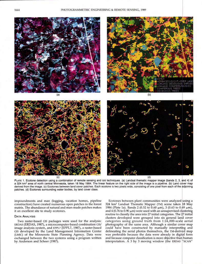
~ ~PLATE 1. Ecotone detection using a combination of remote sensing and GIS techniques. (a) Landsat thematic mapper image (bands 2, 3, fnd 4) ofa 324 km2 area of north central Minnesota, taken 18 May 1984. The linear feature on the right side of the image is a pipeline. (b) Land c9ver mapderived from the image. (c) Ecotones between land cover patches. Each ecotone is two pixels wide, consisting of one pixel from each of the djoiningpatches. (d) Ecotones surrounding water bodies, by land cover class.

impoundments and man (logging, vacation homes, pipelineconstruction) have created numerous open patches in the forestmatrix. The abundance of natural and man-made patches makesit an excellent site to study ecotones.

DATA ANALYSIS

Two raster-based GIS packages were used for the analysis:ERDAS (ERDAS, 1987), a microcomputer-based combination GIS/image analysis system, and EPPL7 (EPPL7, 1987), a raster-basedGIS developed by the Land Management Information Center(LMIC) of the Minnesota State Planning Agency. Data wereexchanged between the two systems using a program writtenby Anderson and Scheer (1987).

Ecotones between plant communities were analyzed using a324 km2 Landsat Thematic Mapper (TM) scene taken 8 May1984 (Plate 1a). Bands 2 (0.52 to 0.60 !-Lm), 3 (0.63 to O. 9 !-Lm),and 4 (0.76 to 0.90 !-Lm) were used with an unsupervised cl steringroutine to classify the area into 27 initial categories. The 27 initialclusters developed were grouped into six general lantl covercategories using ground truth from 1:24,000-scal aerialphotography of the same area. Although a similar co er mapcould have been constructed by manually interpreti g anddelineating the aerial photos themselves, the TM-deriv d mapwas preferable because the data were already in digi al formand because computer classification is more objective tha humaninterpretation. A 3 by 3 moving window (the ERDAS 'SCAN"

QUANTITATIVE ANALYSIS OF ECOTONES USING A GIS 1645

routin ) was used to smooth the classified image by assigningthe m dal value to the central pixel of each window, therebysmoot ing the image by removing patches < 0.5 ha (Plate Ib).

The moving window was also used to locate boundariesbetwe n the land cover classes. The data layer was scannedwith a 3 by 3 pixel moving window using the boundary optionof the EROAS SCAN routine. A value of 0 was assigned to anynon-b undary pixel, and the value of the land cover class topixels t the boundaries of the land cover patches. The resultingbound ries were two pixels wide, showing the land cover classesprese on both sides of each ecotone (Plate Ie).

Whi e the above analysis provided a good graphical depictionof eco one location and type, it could not be used to classifyboun ries according to the types of land cover classes whichthey s parated. This was accomplished by creating a separatedata 1 er for each land cover class. As each cover was selected,all ot er cover types were recoded to O. A one-pixel buffersurrou ding each polygon in the selected cover class was createdwith t e EROAS "SEARCH" command, and used to extract datafrom t e original cover map with the EROAS "MATRIX" command.The r ult was an edge map of all land cover types adjoiningpolyg ns of the selected cover type (Plate Id).

Eco nes between areas of high and low vegetation biomasswere nalyzed using the same Landsat scene. A normalizeddiffer ce vegetation index (NOVI), which is related to greenveget ion biomass (Tucker, 1979), was computed for each pixelin the mage (Figure la) using the following formula:

NOVl = (x4 - x2)/((x4 + x2) + 0.5)

where NOVI = normalized difference vegetation index,x4 = brightness value from infrared band 4, andx2 = brightness value from red band 2.

Ecoto es between areas of high NOVI (i.e., high biomass) andlow N VI (Le., low biomass) were determined using EPPL7 toscan t e resultant image with a 3 by 3 pixel moving windowwhich assigned the difference between the maximum andmini m value in the window to the central pixel, thusidenti ing areas of high NOVI contrast (Figure Ib).

RESULTS

Abo t 5,900 krn of ecotones between major vegetation typeswere etected using the land cover data layer generated bymean of satellite data analysis (Table 1). Patches of coniferoustrees ad the longest cumulative boundary length (1,550 krn),follow d by muskeg (1,173 krn) and herbaceous patches (1,059krn). he four longest individual boundary classes were alsobetwe n conifers and other land cover types: conifer/muskeg,conife /deciduous, conifer/shrub, and coniferlherbaceous (Table1). Th' was expected, based on the predominance of the coniferland ever type (Plate Ib).

Eco nes with water bodies had the shortest cumulative length,270 . It is interesting to note, however, that water bodiesshare ore border with lowland shrub patches than with anyother over type, even though all other boundary classes have

,longe cumulative lengths than that of lowland shrubs. Thelengt of water/shrub ecotone is approximately twice the lengthof wa er/deciduous ecotone, despite the fact that shrub anddecid ous forest patches had equivalent total ecotone lengths.This i dicates a preferential association between water and low­land ciduous shrubs. At a broader scale, the lowland decid­uous hrub patches constitute an ecotone between water anduplan .

Who e the above technique was useful for detecting, classi­fying, and measuring ecotone length, it provided no informa­tion a out relative differences in the ecological properties ofadjace t patches. For example, there is a large difference in thebioma s of a lake as opposed to a forest, so the ecotone between

(b)FIG. 1. (a) Vegetation index computed from bands 2 and 4 of a Landsatthematic mapper image of north central Minnesota (Plate 1a). High in­tensity pixels have high NOVI values. (b) Ecotones between areas of highand low vegetation productivity derived by scanning the above image.High intensity pixels occur where the contrast among NOVI values in the3 by 3 pixel scan window was greatest.

these two classes would be a high contrast ecotone (Holland,1988). Scanning the NOVI image with a maximum-minimumwindow provided a measure of ecotone contrast, with low val­ues signifying homogeneity within the window (i.e., no eco­tone) and high values signifying large differences in NOVI withinthe window (Le., a high contrast ecotone). Therefore, ecotonesbetween lakes and upland forest appear as bright borders onthe scanned NOVI image, while the lakes themselves and areasof homogenous muskeg vegetation are uniformly dark due tothe lack of variation among NOVI values. Other distinct bound­aries detected by this technique include boundaries between

1646 PHOTOGRAMMETRIC ENGINEERING & REMOTE SENSING, 1989

TABLE 1. LENGTH OF BOUNDARIES BE1WEEN DIFFERENT LAND COVER CLASSES SHOWN IN PLATE 1B, BY BOUNDARY TYPE.

Length of boundary (km) with:SHRUB MUSKEG

69 41276 259

152

Water (H20)Herbaceous/cut-over (HERB)Low deciduous shrubs (SHRUB)Low conifers/muskeg (MUSKEG)Coniferous trees (CO IF)Deciduous trees (DECID)Total boundary length (km)Percent of total boundary

H20

2704%

HERB65

105918%

92316%

117320%

CONIF DECI61 35

314 145375 50411 311

389

1550 93126% 16%

areas of upland forest (high biomass) and lowland deciduousshrubs or herbaceous areas (Figure Ib) (low biomass).

DISCUSSION

We found that analysis of remotely sensed 'imagery using araster-based GIS provided ecotone detection and quantificationcapabilities which would have been more difficult to impossiblewithout a GIS. While ecotones between land cover types can bedetected by conventional mapping methods (e.g., field surveys,air photo interpretation, delimiting vegetation range maps), GISanalysis of remotely sensed imagery was more objective thanconventional methods. Both conventional and GIS methods maybe equally effective at detecting ecotones in areas where themagnitude of ecological change is large and abrupt, but the GISalso detected ecological transitions which were more subtle,such as those between different forest types. A GIS is also morelikely to detect ecotones surrounding small patches which wouldbe difficult and time-consuming to delineate manually.

Conventional vegetation maps generally differentiate dissim­ilar ecological patches, rather than characterize the ecotonesthemselves. Although the boundaries drawn on the maps con­stitute ecotones, only the patch contents are classified andquantified. The GIS provided the ability to classify ecotones bythe cover types which they separated, and to measure the lengthof those different ecotone classes. While we used remotely sensedimagery as our source data, the moving window boundaryanalysis could be applied to any rasterized map with nominaldata, such as land cover maps in the USGS LUDA series.

This ecotone analysis provided new insights about the asso­ciation of different land cover types (i.e., water and lowlanddeciduous shrubs). The application of statistical techniques, suchas electivity index, to these data could provide a more quanti­tative analysis of the strength of ecological associations and di­sassociations between cover types (Pastor and Broschart, 1989).

The moving window approach was also applicable to raster­ized interval data, in this case the NDVI data layer. Not onlywas this approach suitable for locating ecotones, it also pro­vided a measure of ecotone contrast. This could be used toidentify areas where fluxes across ecotones may be important.For example, input of allochthonous organic matter fom uplandto stream constitutes a large proportion of the stream's carbonbudget, due to the stream's inherently low productivity relativeto upland ecosystems. Therefore, high contrast ecotones on thescanned NDVI image, such as those between water and upland,may indicate areas of high biomass flux between ecosystems.

We analyzed a single date of imagery, but the moving win­dow technique could be used with a time series of images todetermine boundary stability. For instance, the ecotones be­tween different land cover types (Plate Ie) are relatively stableon an annual basis, changing only with disturbance. Someboundaries may be more ephemeral, however, such as the dif­ference in NDVI between lowland deciduous shrubs and uplandforest. Upland vegetation greens up faster in the spring thandoes wetland vegetation, so biomass ecotones detected using

an 18 May 1984 image would probably diminish later in thegrowing season as wetland biomass approaches that of 'ts up­land counterparts. By integrating NOVI values over an entiregrowing season, ecotones between areas of high and 1 w netprimary productivity (i.e., process-related ecotones) co Id beidentified (Goward et aI., 1986).

Where the locations of ecological boundaries are treadyknown, GIS techniques can be used to characterize eco ystemproperties adjacent to the boundary, such as land cove adja­cent to streams. This buffering technique has been co binedwith field data to investigate the effect of streamside la d useson stream water quality Oohnston et aI., 1988; Osbor e andWiley, 1988).

Ecotone classification and measurement is operationall muchsimpler using a vector-based than a raster-based GIS. ector­based systems such as ARC/INFO automatically determine whichpolygons adjoin an ecotone when topology is created or thecoverage. Ecotone lengths can therefore easily be sum arizedby the land cover classes which they separate. The adv ntageof using raster-based systems, however, is that they c n useimage analysis to detect ecotones, while ecotone locati n in avector-based system is pre-determined by the input dat (i.e.,the digitized linework). Furthermore, raster-based GISs an beused with interval data to analyze ecotone contrast, a ca abilitylacking in vector-based systems.

The resurgence of interest in ecotones has come at tech­nologically opportune time. The evolution of GIS equipm t andmethods over the past decade have greatly increased our abilityto quantitatively study ecotones. This ability will be esse tial tothe development and testing of scientific theories pertai ing toecotones.

ACKNOWLEDGMENTS

The University of Minnesota Remote Sensing Laborato y pro­vided the Landsat Thematic Mapper image used. This s con­tribution number 49 of the Center for Water and the Enviro ent,and 6 of the NRRl Geographic Information Laboratory (NS grantno. DIR-8805437).

REFERENCES

Anderson, K. L., and B. W. Scheer, 1987. A Program to Exchangeand EPPL7 Data Files. Water Resources Research Ctr. Tech.University of Minnesota, St. Paul, Minnesota.

Clements, F. c., 1905. Research Methods in Ecology. University Pu lishingCompany, Lincoln, Nebraska.

Curtis, J. T., 1959. The Vegetation of Wisconsin. University of Wi consinPress, Madison, Wisconsin.

Dasmann, R. F., 1964. Wildlife Biology. Wiley, New York.di Castri, F., A. Hansen, and M. M. Holland, 1988. A New Look at

Ecotones: Emerging International Projects on Landscape Bounda ies. Bi­ology International, Special Issue 17.

EPPL7, 1987. EPPL7 Users Guide, Version 7, Release 1.1 Minneso a StatePlanning Agency, St. Paul, Minnesota.

QUANTITATIVE ANALYSIS OF ECOTONES USING A GIS 1647

ERDAS, 1987. ERDA Users Guide. ERDAS, Inc. Atlanta, Georgia.Goward S. N., C. J. Tucker, and D. G. Dye, 1986. North American

veg tation patterns observed with meteorological satellite data.Cou ling of Ecological Studies with Remote Sensing: Potentials at FourBios here Reserves in the United States. (M.1. Dyer and D.A. Crossley,Jr., ds) U.S. Man and the Biosphere Program, Department of State,Wa ington, D.C., pp. 96-115.

Holland M. M. (compiler), 1988. SCOPE/MAB Technical Consultations onLan cape Boundaries. Biology International Special Issue 17:46-104.

Johnsto C. A., and R. J. Naiman, 1989. The use of a geographic in­for ation system to analyze long-term landscape alteration by bea­ver. Landscape Ecology (in press).

Johnsto C. A., N. E. Detenbeck, J. P. Bonde, and G. J. Niemi, 1988.Geo aphic information systems for cumulative impact assess­

. Photogrammetric Engineering & Remote Sensing 54: 1609-1615.C. A., J. Pastor, and G. Pinay, 1989. Quantitative methods

for tudying landscape boundaries. Landscape boundaries: conse­quen es for biotic diversity and ecological flows. (F. di Castri and A.Ha en, editors). SCOPE Series (in press).

Krumm ,J. R., R. H. Gardner, G. Sugihara, R. V. O'Neill, and P. R.Col an, 1987. Landscape patterns in a disturbed environment.Oik 48: 321-324.

Leopold A., 1933. Game Management. Schriber, New York.Mohler, . R. J., G. L. Wells, C. R. Hallum, and M. H. Trenchard, 1986.

Monitoring vegetation of drought environments. BioScience 36:478­483.

Nellis, M. D., and J. M. Briggs, 1989. The effect of spatial scale on Konzalandscape classification using textural analysis. Landscape Ecology2:93-100.

Odum, E. P., 1971. Fundamentals of Ecology, third edition. W.B. Saun­ders, Philadelphia, Pennsylvania.

Omernik, J. M., 1986. Ecoregions of the Conterminous United States Map(scale 1:7,500,000). U.S. Environmental Protection Agency, Corval­lis Environmental Research Laboratory, Corvallis, Oregon.

Osborne, L. L., and M. J. Wiley, 1988. Empirical relationships betweenland uselcover and stream water quality in an agricultural wa­tershed. ]. Environ. Manage. 26: 9-27.

Pastor, J., and M. Broschart, 1989. The spatial pattern of a northernconifer-hardwood landscape. Landscape Ecology (in press).

Pickett, S. T. A., and P. S. White (editors), 1985. The Ecology of NaturalDisturbance and Patch Dynamics. Academic Press, Orlando, Florida.

Tomlin, C. D., 1983. Digital Cartographic Modeling Techniques in Environ­mental Planning. Doctoral Dissertation, Yale University, School ofForestry and Environmental Planning, New Haven, Conn.

Tucker, C. J., 1979. Red and photographic linear combinations for mon­itoring vegetation. Remote Sensing of Environment 8: 127-150.

Tucker, C. J., J. R. G. Townshend, and T. E. Goff, 1985. African land­cover classification using satellite data. Science 227: 369-375.

CALL OR WRITE FOR QUANTITY PRICES.

Lumin AERO-RC papers designed for use withautom ic printers and processors as well as tray developing. In 10 x 10 to 30 x 40inches n cut sheets, and rolls 9 3/8 to 49 '/2 inches. In Semi-matte, Glossy, Pearland M ral R, at low, low prices. Price list and samples available.

Introdu ing Air Photo's NEW dual-range mirror stereoscope with 1.8 magnification.The M del #F77A dual-range mirror stereoscope is an indispensable tool for surveysin agri ulture, forestry, civil engineering, architecture and other photogrammetricapplic ions. State of the Art optics, sturdy construction and convenience featuresmake ir Photo's F77A a very desirable addition to your photogrammetric instrumentsat a ve y competitive price.

DUO-Range Mirror~ Stereoscope

~

RESIN-COATED PAPERPRODUCES PRINTS OF

INCREDIBLE DETAILinos c§RO-§:>Lu

QUANTITY PRICE LIST FORPOCKET STEREOSCOPES

NEW PS-4 PS-2A Postage &FOUR POWER TWO POWER Handling'

EACH EACH EACHau NTITY

12t 56 t 11

12 a d up

35.5029.5028.5025.75

225018.9517.9513.55

4.751.751.251.00

TWO MODELS PS-2a & PS·4POCKET STEROSCOPES

Strong cast alloy, crackle finish 50mm to 75mm inter­pupillary adjustment. Firmly locking fold away legs.Factory coated genuine glass optics. Lined-vinyl caseincluded immediate delivery. Choose PS-2a or PS-4

TELEX# 13-1575

\\

.\ ~

\ \\/

AI PHOTO SUPPLY CORP. P.O. BOX 158 SOUTH STATION, YONKERS NY. 10705-0158 DEPT,119 FAX# 914-965-0367CALL TOLL FREE 800-759-3957 EXCEPT HAWAII & ALASKA, YONKERS# 914-965-4630.