Remote Sens. 2013, 5, 5209-5264; doi:10.3390/rs5105209 Remote Sensing ISSN 2072-4292 www.mdpi.com/journal/remotesensing Article Quality Assessment of Pre-Classification Maps Generated from Spaceborne/Airborne Multi-Spectral Images by the Satellite Image Automatic Mapper™ and Atmospheric/Topographic Correction™-Spectral Classification Software Products: Part 2 — Experimental Results Andrea Baraldi 1, *, Michael Humber 1 and Luigi Boschetti 2 1 Department of Geographical Sciences, University of Maryland, 4321 Hartwick Rd, Suite 209, College Park, MD 20740, USA; E-Mail: [email protected] 2 College of Natural Resources, University of Idaho, 875 Perimeter Drive, Moscow, ID 83844, USA; E-Mail: [email protected] * Author to whom correspondence should be addressed; E-Mail: [email protected]; Tel.: +1-301-314-1467; Fax: +1-301-405-6806. Received: 1 July 2013; in revised form: 17 September 2013 / Accepted: 9 October 2013 / Published: 18 October 2013 Abstract: This paper complies with the Quality Assurance Framework for Earth Observation (QA4EO) international guidelines to provide a metrological/statistically-based quality assessment of the Spectral Classification of surface reflectance signatures (SPECL) secondary product, implemented within the popular Atmospheric/Topographic Correction (ATCOR™) commercial software suite, and of the Satellite Image Automatic Mapper™ (SIAM™) software product, proposed to the remote sensing (RS) community in recent years. The ATCOR™-SPECL and SIAM™ physical model-based expert systems are considered of potential interest to a wide RS audience: in operating mode, they require neither user-defined parameters nor training data samples to map, in near real-time, a spaceborne/airborne multi-spectral (MS) image into a discrete and finite set of (pre-attentional first-stage) spectral-based semi-concepts (e.g., “vegetation”), whose informative content is always equal or inferior to that of target (attentional second-stage) land cover (LC) concepts (e.g., “deciduous forest”). For the sake of simplicity, this paper is split into two: Part 1—Theory and Part 2—Experimental results. The Part 1 provides the present Part 2 with an interdisciplinary terminology and a theoretical background. To comply with the principle of statistics and the QA4EO guidelines discussed in the Part 1, OPEN ACCESS

Welcome message from author
This document is posted to help you gain knowledge. Please leave a comment to let me know what you think about it! Share it to your friends and learn new things together.
Transcript
Remote Sens. 2013, 5, 5209-5264; doi:10.3390/rs5105209
Remote Sensing ISSN 2072-4292
www.mdpi.com/journal/remotesensing
Article
Quality Assessment of Pre-Classification Maps Generated from Spaceborne/Airborne Multi-Spectral Images by the Satellite Image Automatic Mapper™ and Atmospheric/Topographic Correction™-Spectral Classification Software Products: Part 2 — Experimental Results
Andrea Baraldi 1,*, Michael Humber 1 and Luigi Boschetti 2
1 Department of Geographical Sciences, University of Maryland, 4321 Hartwick Rd, Suite 209,
College Park, MD 20740, USA; E-Mail: [email protected] 2 College of Natural Resources, University of Idaho, 875 Perimeter Drive, Moscow, ID 83844, USA;
E-Mail: [email protected]
* Author to whom correspondence should be addressed; E-Mail: [email protected];
Tel.: +1-301-314-1467; Fax: +1-301-405-6806.
Received: 1 July 2013; in revised form: 17 September 2013 / Accepted: 9 October 2013 /
Published: 18 October 2013
Abstract: This paper complies with the Quality Assurance Framework for Earth Observation
(QA4EO) international guidelines to provide a metrological/statistically-based quality
assessment of the Spectral Classification of surface reflectance signatures (SPECL)
secondary product, implemented within the popular Atmospheric/Topographic Correction
(ATCOR™) commercial software suite, and of the Satellite Image Automatic Mapper™
(SIAM™) software product, proposed to the remote sensing (RS) community in recent
years. The ATCOR™-SPECL and SIAM™ physical model-based expert systems are
considered of potential interest to a wide RS audience: in operating mode, they require
neither user-defined parameters nor training data samples to map, in near real-time, a
spaceborne/airborne multi-spectral (MS) image into a discrete and finite set of
(pre-attentional first-stage) spectral-based semi-concepts (e.g., “vegetation”), whose
informative content is always equal or inferior to that of target (attentional second-stage)
land cover (LC) concepts (e.g., “deciduous forest”). For the sake of simplicity, this paper is
split into two: Part 1—Theory and Part 2—Experimental results. The Part 1 provides the
present Part 2 with an interdisciplinary terminology and a theoretical background. To
comply with the principle of statistics and the QA4EO guidelines discussed in the Part 1,
OPEN ACCESS
Remote Sens. 2013, 5 5210
the present Part 2 applies an original adaptation of a novel probability sampling protocol
for thematic map quality assessment to the ATCOR™-SPECL and SIAM™ pre-classification
maps, generated from three spaceborne/airborne MS test images. Collected metrological/
statistically-based quality indicators (QIs) comprise: (i) an original Categorical Variable
Pair Similarity Index (CVPSI), capable of estimating the degree of match between a test
pre-classification map’s legend and a reference LC map’s legend that do not coincide and
must be harmonized (reconciled); (ii) pixel-based Thematic (symbolic, semantic) QIs
(TQIs) and (iii) polygon-based sub-symbolic (non-semantic) Spatial QIs (SQIs), where all
TQIs and SQIs are provided with a degree of uncertainty in measurement. Main
experimental conclusions of the present Part 2 are the following. (I) Across the three test
images, the CVPSI values of the SIAM™ pre-classification maps at the intermediate and
fine semantic granularities are superior to those of the ATCOR™-SPECL single-granule
maps. (II) TQIs of both the ATCOR™-SPECL and the SIAM™ tend to exceed
community-agreed reference standards of accuracy. (III) Across the three test images and
the SIAM™’s three semantic granularities, TQIs of the SIAM™ tend to be significantly
higher (in statistical terms) than the ATCOR™-SPECL’s. Stemming from the proposed
experimental evidence in support to theoretical considerations, the final conclusion of this
paper is that, in compliance with the QA4EO objectives, the SIAM™ software product can be
considered eligible for injecting prior spectral knowledge into the pre-attentive vision first
stage of a novel generation of hybrid (combined deductive and inductive) RS image
understanding systems, capable of transforming large-scale multi-source multi-resolution EO
image databases into operational, comprehensive and timely knowledge/information products.
Keywords: attentive vision; confusion matrix; degree of uncertainty in measurement;
harmonization (reconciliation) of ontologies; land cover classification; multi-spectral image;
overlapping area matrix; pre-attentive vision; preliminary classification; probability sampling;
quality indicators of operativeness; categorical and spatial accuracy of thematic maps
Acronyms and Abbreviations
ADS: Airborne Digital Scanner
ATCOR™: Atmospheric/Topographic Correction™
ASQI: Average Spatial Quality Indicator
B: (Visible) Blue
CEOS: Committee on Earth Observation Satellites
CMTRX: (Square and sorted) Confusion Matrix
CVPSI: Categorical Variable Pair Similarity Index
EO: Earth Observation
FEOQI: Fuzzy Edge Overlap Spatial Quality Indicator
G: (Visible) Green
GEOBIA: Geographic Object-Based Image Analysis
Remote Sens. 2013, 5 5211
GEOOIA: Geographic Object-Observation Image Analysis
GEOROI: Geographic Region Of Interest
GIS: Geographic Information System
HR: High Resolution
HRVIR: High Resolution Visible & Infrared
IR: Infra-Red
IRS: Indian Remote sensing Satellite
LAI: Leaf Area Index
LC: Land Cover
LCC: Land Cover Change
LISS: medium resolution Linear Imaging Self-Scanner
MIR: Medium infra-red
MODIS : Moderate Resolution Imaging Spectroradiometer
MS: Multi-Spectral
OAMTRX: Overlapping Area Matrix
OSQI: Oversegmentation Spatial Quality Indicator
QA4EO: Quality Accuracy Framework for Earth Observation
QI: Quality Indicator
QIO: Quality Indicator of Operativeness
Q-SIAM™: QuickBird-like Satellite Image Automatic Mapper™
R: (visible) Red
RS: Remote Sensing
RS-IUS: Remote Sensing Image Understanding System
SIAM™: Satellite Image Automatic Mapper™
SIRS: Simple random sampling
SPECL: Spectral Classification of surface reflectance signatures
SPOT: Satellite Pour l'Observation de la Terre
SQI: Spatial Quality Indicator
S-SIAM™: SPOT-like Satellite Image Automatic Mapper™
SURF: Surface Reflectance
TIR: Thermal Infra-Red
TM: Trademark
TO: Target image-Object
TOA: Top-Of-Atmosphere
TOARF: Top-Of-Atmosphere Reflectance
TQI: Thematic Quality Indicator
USGS: US Geological Survey
USQI: Undersegmentation Spatial Quality Indicator
VHR: Very High Resolution
Remote Sens. 2013, 5 5212
1. Introduction
One visionary goal of the Quality Assurance Framework for Earth Observation (QA4EO)
guidelines, delivered by the international Group on Earth Observations (GEO)-Committee on Earth
Observation Satellites (CEOS) [1,2], is to develop information processing systems capable of transforming
automatically, i.e., without user interactions, large-scale multi-source multi-resolution Earth observation
(EO) image databases into “operational, comprehensive and timely knowledge/information
products” [1–3], at spatial extents ranging from local to global scale [4].
In compliance with the QA4EO guidelines [2], this paper pursues a quality assessment of two
operational (turnkey) software products, suitable for automatic preliminary classification
(pre-classification [5]) of spaceborne/airborne Earth Observation (EO) multi-spectral (MS) images: the
Spectral Classification of surface reflectance signatures (SPECL) and the Satellite Image Automatic
Mapper™ (SIAM™). The former is implemented as a non-validated secondary product within the
popular Atmospheric/Topographic Correction™ (ATCOR™)-2/3/4 commercial software toolbox [6–9].
The latter has been presented in recent years in the remote sensing (RS) literature [10–19], where
enough information is provided for the SIAM™ implementation to be reproduced [11,17].
To the best of these authors' knowledge, the ATCOR™-SPECL and SIAM™ software products are,
to date, the only two pre-attentive vision expert systems (deductive inference systems for pre-attentional
vision) in operating mode made available to the RS community for “fully automatic” near real-time
pre-classification of radiometrically calibrated spaceborne/airborne MS images, irrespective of their
spatial resolution. The term “pre-attentive vision” is used herein as a synonym of “low-level vision”,
according to the terminology of neural science [5,10–19] (refer to the Part 1, Section 2.3 [20]). “Fully
automatic” means that the information processing system requires neither user-defined parameters nor
training data samples to run [21] (refer to the Part 1, Section 4.1 [20]).
For the sake of simplicity this paper is split into two: Part 1—Theory [20] and
Part 2—Experimental results.
The Part 1 of this paper provides the present Part 2 with an interdisciplinary terminology
and a theoretical background [20]. To cope with cognitive problems [22,23], like RS image
understanding [24,25], the proposed terminology encompasses multiple disciplines, like philosophical
hermeneutics [26,27], machine learning [22,23], artificial intelligence [28,29], computer vision [30]
and human vision [5], in addition to the traditional RS jargon [31] (refer to the Part 1, Section 2 [20]).
Based on theoretical considerations exclusively, the Part 1 concludes that the proposed assessment and
comparison of the ATCOR™-SPECL and SIAM™ deductive pre-classifiers is appropriate, well-timed
and of potential interest to a large portion of the RS readership.
To comply with the principles of statistics and the QA4EO guidelines [1,2], recalled in the
Part 1 [20], and with the GEO-CEOS land product accuracy validation criteria [3], the present Part 2 of
this paper applies a novel probability sampling protocol for thematic map quality assessment, selected
from the existing literature [32], to the ATCOR™-SPECL and SIAM™ pre-classification maps
generated from three spaceborne/airborne MS test images. Main characteristics of the proposed
probability sampling protocol are that [32]: (i) it introduces a novel Categorical Variable Pair
Similarity Index (CVPSI) ∈ [0, 1], able to assess the degree of match between a pair of reference and
test thematic map legends which, in general, do not coincide and must be harmonized before
Remote Sens. 2013, 5 5213
comparison, (ii) its sample estimates are statistically valid (refer to the Part 1, Section 2.6 [20]) [24,25],
(iii) two independent sets of metrological/statistically-based quality indicators (QIs) are generated from
the test thematic map, namely, pixel-based thematic (semantic, categorical) quality indicators (TQIs)
and polygon-based sub-symbolic (asemantic) spatial quality indicators (SQIs), and (iv) TQIs and SQIs
are statistically significant, i.e., they are provided with a degree of uncertainty in measurement, in
compliance with the principles of statistics and the QA4EO guidelines (refer to the Part 1,
Section 3 [20]).
Stemming from experimental evidence collected in the Part 2 and supported by theoretical
considerations presented in the Part 1, conclusions of this paper may have an impact on the design and
implementation of a novel generation of hybrid (combined deductive and inductive) RS image
understanding systems (RS-IUSs) in operating mode, capable of coping with large-scale multi-source
multi-resolution RS image databases [10–20].
The rest of the present Part 2 is organized as follows. Section 2 presents the test data set.
In Section 3, a probability sampling protocol is proposed for quality assessment of the ATCOR™-SPECL
and SIAM™ pre-classification maps generated from the test image set. Section 4 reports on the
comparison of QIs of operativeness (QIOs) estimated from the ATCOR™-SPECL and SIAM™
software products in operating mode. Conclusions are reported in Section 5. The Appendix presents
two different formulations of the CVPSI.
2. Test Image Set
To assess the accuracy of pre-classification maps of EO images acquired across time, space and MS
imaging sensors, two spaceborne high resolution (HR) MS test images and one airborne very high
resolution (VHR) MS test image are selected and radiometrically calibrated, in accordance with: (i) the
input data constraints of physical models (refer to the Part 1, Section 2.2 [20]), (ii) the calibration/
validation (Cal/Val) requirements of the QA4EO guidelines (refer to the Part 1, Section 3 [20]) and
(iii) the GEO-CEOS land product accuracy validation criteria [3] (refer to Section 1). The three EO test
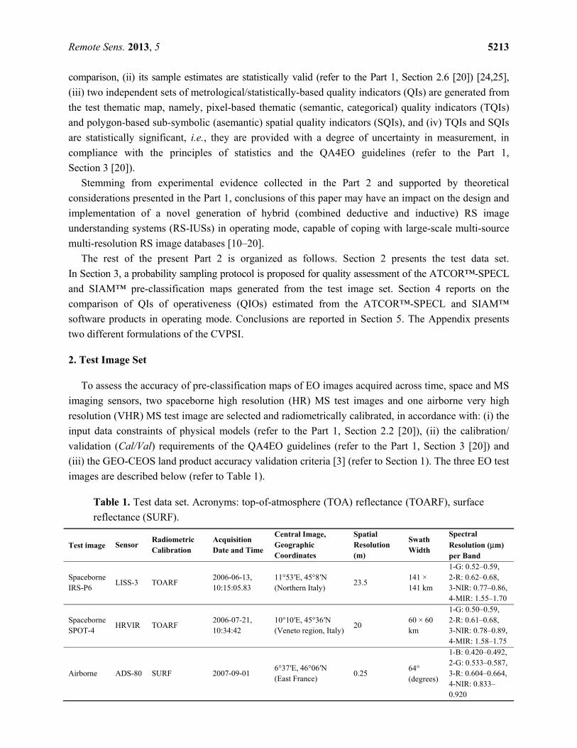
images are described below (refer to Table 1).
Table 1. Test data set. Acronyms: top-of-atmosphere (TOA) reflectance (TOARF), surface
reflectance (SURF).
Test image Sensor Radiometric Calibration
Acquisition Date and Time
Central Image, Geographic Coordinates
Spatial Resolution (m)
Swath Width
Spectral
Resolution (μm) per Band
Spaceborne IRS-P6
LISS-3 TOARF 2006-06-13, 10:15:05.83
11°53′E, 45°8′N (Northern Italy)
23.5 141 × 141 km
1-G: 0.52–0.59, 2-R: 0.62–0.68, 3-NIR: 0.77–0.86, 4-MIR: 1.55–1.70
Spaceborne SPOT-4
HRVIR TOARF 2006-07-21, 10:34:42
10°10′E, 45°36′N (Veneto region, Italy)
20 60 × 60 km
1-G: 0.50–0.59, 2-R: 0.61–0.68, 3-NIR: 0.78–0.89, 4-MIR: 1.58–1.75
Airborne ADS-80 SURF 2007-09-01 6°37′E, 46°06′N (East France)
0.25 64° (degrees)
1-B: 0.420–0.492, 2-G: 0.533–0.587, 3-R: 0.604–0.664, 4-NIR: 0.833–0.920
Remote Sens. 2013, 5 5214
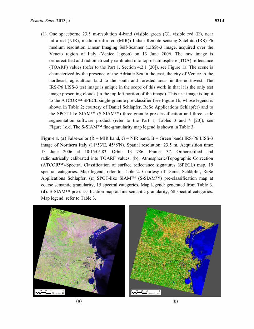
(1). One spaceborne 23.5 m-resolution 4-band (visible green (G), visible red (R), near
infra-red (NIR), medium infra-red (MIR)) Indian Remote sensing Satellite (IRS)-P6
medium resolution Linear Imaging Self-Scanner (LISS)-3 image, acquired over the
Veneto region of Italy (Venice lagoon) on 13 June 2006. The raw image is
orthorectified and radiometrically calibrated into top-of-atmosphere (TOA) reflectance
(TOARF) values (refer to the Part 1, Section 4.2.1 [20]), see Figure 1a. The scene is
characterized by the presence of the Adriatic Sea in the east, the city of Venice in the
northeast, agricultural land to the south and forested areas in the northwest. The
IRS-P6 LISS-3 test image is unique in the scope of this work in that it is the only test
image presenting clouds (in the top left portion of the image). This test image is input
to the ATCOR™-SPECL single-granule pre-classifier (see Figure 1b, whose legend is
shown in Table 2; courtesy of Daniel Schläpfer, ReSe Applications Schläpfer) and to
the SPOT-like SIAM™ (S-SIAM™) three-granule pre-classification and three-scale
segmentation software product (refer to the Part 1, Tables 3 and 4 [20]), see
Figure 1c,d. The S-SIAM™ fine-granularity map legend is shown in Table 3.
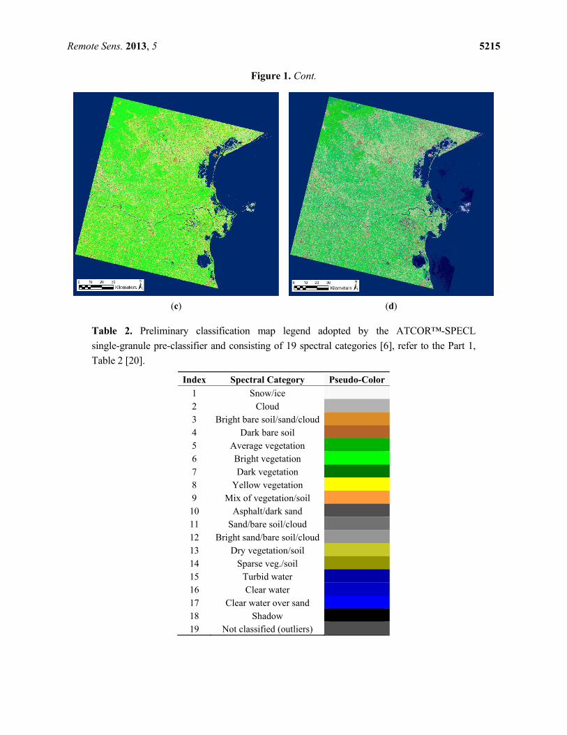
Figure 1. (a) False-color (R = MIR band, G = NIR band, B = Green band) IRS-P6 LISS-3
image of Northern Italy (11°53′E, 45°8′N). Spatial resolution: 23.5 m. Acquisition time:
13 June 2006 at 10:15:05.83. Orbit: 13 786. Frame: 37. Orthorectified and
radiometrically calibrated into TOARF values. (b): Atmospheric/Topographic Correction
(ATCOR™)-Spectral Classification of surface reflectance signatures (SPECL) map, 19
spectral categories. Map legend: refer to Table 2. Courtesy of Daniel Schläpfer, ReSe
Applications Schläpfer. (c): SPOT-like SIAM™ (S-SIAM™) pre-classification map at
coarse semantic granularity, 15 spectral categories. Map legend: generated from Table 3.
(d): S-SIAM™ pre-classification map at fine semantic granularity, 68 spectral categories.
Map legend: refer to Table 3.
(a) (b)
Remote Sens. 2013, 5 5215
Figure 1. Cont.
(c) (d)
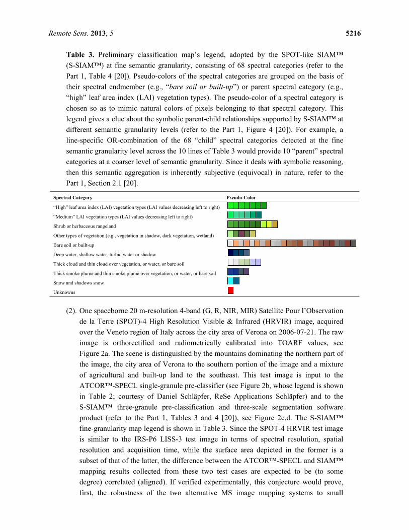
Table 2. Preliminary classification map legend adopted by the ATCOR™-SPECL
single-granule pre-classifier and consisting of 19 spectral categories [6], refer to the Part 1,
Table 2 [20].
Index Spectral Category Pseudo-Color
1 Snow/ice 2 Cloud 3 Bright bare soil/sand/cloud4 Dark bare soil 5 Average vegetation 6 Bright vegetation 7 Dark vegetation 8 Yellow vegetation 9 Mix of vegetation/soil 10 Asphalt/dark sand 11 Sand/bare soil/cloud 12 Bright sand/bare soil/cloud13 Dry vegetation/soil 14 Sparse veg./soil 15 Turbid water 16 Clear water 17 Clear water over sand 18 Shadow 19 Not classified (outliers)
Remote Sens. 2013, 5 5216
Table 3. Preliminary classification map’s legend, adopted by the SPOT-like SIAM™
(S-SIAM™) at fine semantic granularity, consisting of 68 spectral categories (refer to the
Part 1, Table 4 [20]). Pseudo-colors of the spectral categories are grouped on the basis of
their spectral endmember (e.g., “bare soil or built-up”) or parent spectral category (e.g.,
“high” leaf area index (LAI) vegetation types). The pseudo-color of a spectral category is
chosen so as to mimic natural colors of pixels belonging to that spectral category. This
legend gives a clue about the symbolic parent-child relationships supported by S-SIAM™ at
different semantic granularity levels (refer to the Part 1, Figure 4 [20]). For example, a
line-specific OR-combination of the 68 “child” spectral categories detected at the fine
semantic granularity level across the 10 lines of Table 3 would provide 10 “parent” spectral
categories at a coarser level of semantic granularity. Since it deals with symbolic reasoning,
then this semantic aggregation is inherently subjective (equivocal) in nature, refer to the
Part 1, Section 2.1 [20].
Spectral Category Pseudo-Color
“High” leaf area index (LAI) vegetation types (LAI values decreasing left to right)
“Medium” LAI vegetation types (LAI values decreasing left to right)
Shrub or herbaceous rangeland
Other types of vegetation (e.g., vegetation in shadow, dark vegetation, wetland)
Bare soil or built-up
Deep water, shallow water, turbid water or shadow
Thick cloud and thin cloud over vegetation, or water, or bare soil
Thick smoke plume and thin smoke plume over vegetation, or water, or bare soil
Snow and shadows snow
Unknowns
(2). One spaceborne 20 m-resolution 4-band (G, R, NIR, MIR) Satellite Pour l’Observation
de la Terre (SPOT)-4 High Resolution Visible & Infrared (HRVIR) image, acquired
over the Veneto region of Italy across the city area of Verona on 2006-07-21. The raw
image is orthorectified and radiometrically calibrated into TOARF values, see
Figure 2a. The scene is distinguished by the mountains dominating the northern part of
the image, the city area of Verona to the southern portion of the image and a mixture
of agricultural and built-up land to the southeast. This test image is input to the
ATCOR™-SPECL single-granule pre-classifier (see Figure 2b, whose legend is shown
in Table 2; courtesy of Daniel Schläpfer, ReSe Applications Schläpfer) and to the
S-SIAM™ three-granule pre-classification and three-scale segmentation software
product (refer to the Part 1, Tables 3 and 4 [20]), see Figure 2c,d. The S-SIAM™
fine-granularity map legend is shown in Table 3. Since the SPOT-4 HRVIR test image
is similar to the IRS-P6 LISS-3 test image in terms of spectral resolution, spatial
resolution and acquisition time, while the surface area depicted in the former is a
subset of that of the latter, the difference between the ATCOR™-SPECL and SIAM™
mapping results collected from these two test cases are expected to be (to some
degree) correlated (aligned). If verified experimentally, this conjecture would prove,
first, the robustness of the two alternative MS image mapping systems to small
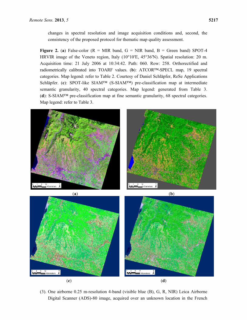
Remote Sens. 2013, 5 5217
changes in spectral resolution and image acquisition conditions and, second, the
consistency of the proposed protocol for thematic map quality assessment.
Figure 2. (a) False-color (R = MIR band, G = NIR band, B = Green band) SPOT-4
HRVIR image of the Veneto region, Italy (10°10′E, 45°36′N). Spatial resolution: 20 m.
Acquisition time: 21 July 2006 at 10:34:42. Path: 060. Row: 258. Orthorectified and
radiometrically calibrated into TOARF values. (b): ATCOR™-SPECL map, 19 spectral
categories. Map legend: refer to Table 2. Courtesy of Daniel Schläpfer, ReSe Applications
Schläpfer. (c): SPOT-like SIAM™ (S-SIAM™) pre-classification map at intermediate
semantic granularity, 40 spectral categories. Map legend: generated from Table 3.
(d): S-SIAM™ pre-classification map at fine semantic granularity, 68 spectral categories.
Map legend: refer to Table 3.
(a) (b)
(c) (d)
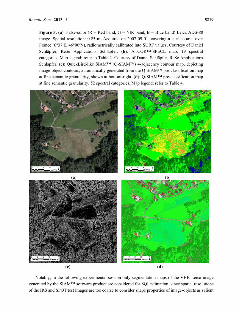
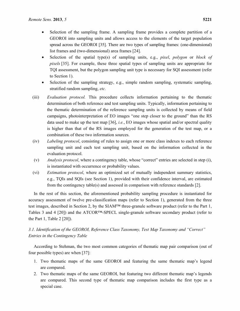
(3). One airborne 0.25 m-resolution 4-band (visible blue (B), G, R, NIR) Leica Airborne
Digital Scanner (ADS)-80 image, acquired over an unknown location in the French
Remote Sens. 2013, 5 5218
Alps on 1 September 2007. The raw MS image is radiometrically calibrated into
surface reflectance (SURF) values, see Figure 3a (courtesy of Daniel Schläpfer, ReSe
Applications Schläpfer). Notably, SURF ⊆ TOARF, i.e., SURF values are a special
case of TOARF values, where SURF ≈ TOARF in very clear sky conditions and flat
terrain conditions [12,32,33] (refer to the Part 1, Section 4.2.1 [20]). In this test case,
visible features include dense tree cover in the southern portion and house
development in the northern portion of the image. This test image is input to the
ATCOR™-SPECL single-granule pre-classifier (see Figure 3b; courtesy of Daniel
Schläpfer, ReSe Applications Schläpfer) and to the QuickBird-like SIAM™
(Q-SIAM™) three-granule pre-classification and three-scale segmentation software
product (refer to the Part 1, Tables 3 and 4 [20]), see Figure 3c,d. The Q-SIAM™
fine-granularity map legend is shown in Table 4.
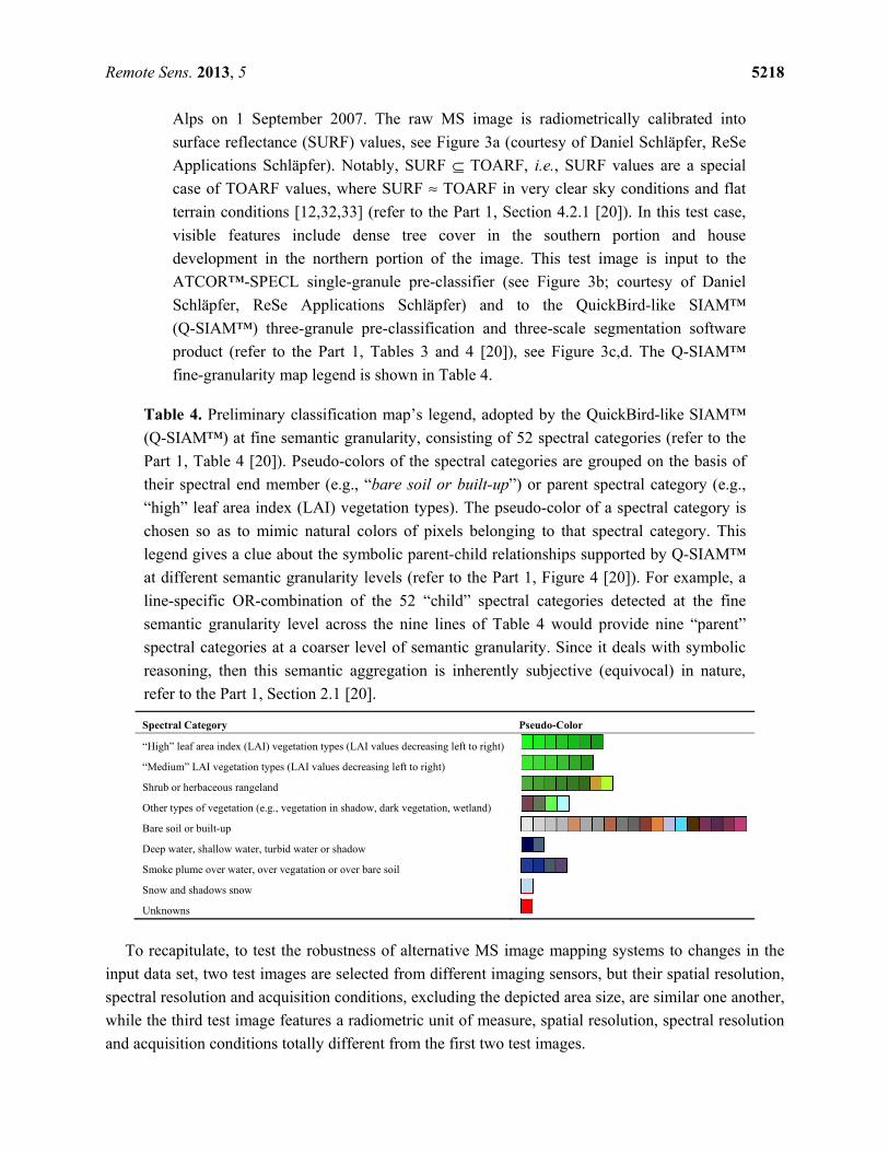
Table 4. Preliminary classification map’s legend, adopted by the QuickBird-like SIAM™
(Q-SIAM™) at fine semantic granularity, consisting of 52 spectral categories (refer to the
Part 1, Table 4 [20]). Pseudo-colors of the spectral categories are grouped on the basis of
their spectral end member (e.g., “bare soil or built-up”) or parent spectral category (e.g.,
“high” leaf area index (LAI) vegetation types). The pseudo-color of a spectral category is
chosen so as to mimic natural colors of pixels belonging to that spectral category. This
legend gives a clue about the symbolic parent-child relationships supported by Q-SIAM™
at different semantic granularity levels (refer to the Part 1, Figure 4 [20]). For example, a
line-specific OR-combination of the 52 “child” spectral categories detected at the fine
semantic granularity level across the nine lines of Table 4 would provide nine “parent”
spectral categories at a coarser level of semantic granularity. Since it deals with symbolic
reasoning, then this semantic aggregation is inherently subjective (equivocal) in nature,
refer to the Part 1, Section 2.1 [20].
Spectral Category Pseudo-Color
“High” leaf area index (LAI) vegetation types (LAI values decreasing left to right)
“Medium” LAI vegetation types (LAI values decreasing left to right)
Shrub or herbaceous rangeland
Other types of vegetation (e.g., vegetation in shadow, dark vegetation, wetland)
Bare soil or built-up
Deep water, shallow water, turbid water or shadow
Smoke plume over water, over vegatation or over bare soil
Snow and shadows snow
Unknowns
To recapitulate, to test the robustness of alternative MS image mapping systems to changes in the
input data set, two test images are selected from different imaging sensors, but their spatial resolution,
spectral resolution and acquisition conditions, excluding the depicted area size, are similar one another,
while the third test image features a radiometric unit of measure, spatial resolution, spectral resolution
and acquisition conditions totally different from the first two test images.
Remote Sens. 2013, 5 5219
Figure 3. (a): False-color (R = Red band, G = NIR band, B = Blue band) Leica ADS-80
image. Spatial resolution: 0.25 m. Acquired on 2007-09-01, covering a surface area over
France (6°37′E, 46°06′N), radiometrically calibrated into SURF values, Courtesy of Daniel
Schläpfer, ReSe Applications Schläpfer. (b): ATCOR™-SPECL map, 19 spectral
categories. Map legend: refer to Table 2. Courtesy of Daniel Schläpfer, ReSe Applications
Schläpfer. (c): QuickBird-like SIAM™ (Q-SIAM™) 4-adjacency contour map, depicting
image-object contours, automatically generated from the Q-SIAM™ pre-classification map
at fine semantic granularity, shown at bottom-right. (d): Q-SIAM™ pre-classification map
at fine semantic granularity, 52 spectral categories. Map legend: refer to Table 4.
(a) (b)
(c) (d)
Notably, in the following experimental session only segmentation maps of the VHR Leica image
generated by the SIAM™ software product are considered for SQI estimation, since spatial resolutions
of the IRS and SPOT test images are too coarse to consider shape properties of image-objects as salient

Remote Sens. 2013, 5 5220
for the recognition of man-made land cover (LC) classes, like “building” and “road”. Since it delivers
as output no segmentation map, the ATCOR™-SPECL commercial software secondary product is not
investigated by SQIs.
3. Probability Sampling Protocol for Thematic Map Accuracy Assessment
An information map, where information is either continuous or categorical (thematic), provides a
reduced representation of a target geospatial population. Map accuracy assessment is an established
component of the process of creating and distributing information maps [24]. The fundamental basis of
a map accuracy assessment protocol is a location-specific comparison, across a geographic region of
interest (GEOROI), between the test map or predicted map to be evaluated [34] and corresponding
ground condition(s) or “reference” condition(s) collected from a target (“true”) geospatial population,
to be univocally identified on the ground [35], which may be represented as a complete-coverage
reference map (also called truth map [34]), if any exists.
Before being used in scientific investigations and policy decisions, thematic or continuous maps
generated from RS images should be: (1) validated by means of probability sampling criteria,
which guarantee statistical consistency (validity) of sample variables [24,25] (refer to the Part 1,
Section 2.6 [20]) and (2) provided with a documented and fully traceable set of mutually uncorrelated,
quantifiable, metrological/statistically-based QIs, featuring a degree of uncertainty in measurement to
be considered statistically significant [2] (refer to the Part 1, Section 3 [20]).
Largely overlooked by the RS community, the two basic requirements of statistical validity and
statistical significance of metrological/statistically-based QIs extracted from RS-IUS’s output products
are almost never satisfied in the RS common practice. This means that, to date, operational qualities,
including mapping accuracy, of existing RS-IUSs remain largely unknown in statistical terms, in
contrast with the principles of statistics and the QA4EO guidelines (refer to the Part 1, Section 2.5 [20]).
In this section, a six-step probability sampling protocol for accuracy assessment of thematic maps
generated from spaceborne/airborne EO images is selected from a related work [32]. The selected
probability sampling protocol is sketched as follows [32].
(i) Identification of the GEOROI, test map taxonomy, reference sample set taxonomy and
“correct” entries in the contingency table (error matrix). A contingency table is the
Cartesian product between two discrete and finite sorted sets of concepts, the test and the
reference vocabulary, which may not coincide. Before the contingency table is instantiated
with probability values, “correct” entries of the contingency table must be selected by a
“knowledge engineer” (domain expert) [28]. Identified as CVPSI ∈ [0, 1] (refer to
Section 1), a metrological QI of the semantic harmonization between the test and reference
map taxonomies is estimated from the distribution of “correct” entries in the contingency table.
(ii) Probability sampling design, where the following decisions must be taken.
• Estimation of the sample set cardinality depending on the project’s requirements
specification in terms of: (i) target overall accuracy and confidence interval, (ii) target
per-class accuracy and confidence interval and (iii) costs of sampling in compliance with
the project budget.
Remote Sens. 2013, 5 5221
• Selection of the sampling frame. A sampling frame provides a complete partition of a
GEOROI into sampling units and allows access to the elements of the target population
spread across the GEOROI [35]. There are two types of sampling frames: (one-dimensional)
list frames and (two-dimensional) area frames [24].
• Selection of the spatial type(s) of sampling units, e.g., pixel, polygon or block of
pixels [35]. For example, these three spatial types of sampling units are appropriate for
TQI assessment, but the polygon sampling unit type is necessary for SQI assessment (refer
to Section 1).
• Selection of the sampling strategy, e.g., simple random sampling, systematic sampling,
stratified random sampling, etc.
(iii) Evaluation protocol. This procedure collects information pertaining to the thematic
determination of both reference and test sampling units. Typically, information pertaining to
the thematic determination of the reference sampling units is collected by means of field
campaigns, photointerpretation of EO images “one step closer to the ground” than the RS
data used to make up the test map [36], i.e., EO images whose spatial and/or spectral quality
is higher than that of the RS images employed for the generation of the test map, or a
combination of these two information sources.
(iv) Labeling protocol, consisting of rules to assign one or more class indexes to each reference
sampling unit and each test sampling unit, based on the information collected in the
evaluation protocol.
(v) Analysis protocol, where a contingency table, whose “correct” entries are selected in step (i),
is instantiated with occurrence or probability values.
(vi) Estimation protocol, where an optimized set of mutually independent summary statistics,
e.g., TQIs and SQIs (see Section 1), provided with their confidence interval, are estimated
from the contingency table(s) and assessed in comparison with reference standards [2].
In the rest of this section, the aforementioned probability sampling procedure is instantiated for
accuracy assessment of twelve pre-classification maps (refer to Section 1), generated from the three
test images, described in Section 2, by the SIAM™ three-granule software product (refer to the Part 1,
Tables 3 and 4 [20]) and the ATCOR™-SPECL single-granule software secondary product (refer to
the Part 1, Table 2 [20]).
3.1. Identification of the GEOROI, Reference Class Taxonomy, Test Map Taxonomy and “Correct”
Entries in the Contingency Table
According to Stehman, the two most common categories of thematic map pair comparison (out of
four possible types) are when [37]:
1. Two thematic maps of the same GEOROI and featuring the same thematic map’s legend
are compared.
2. Two thematic maps of the same GEOROI, but featuring two different thematic map’s legends
are compared. This second type of thematic map comparison includes the first type as a
special case.
Remote Sens. 2013, 5 5222
While the first type of map pair comparisons is by far the most common in the RS literature, in
many practical cases the second type of map pair comparisons occurs, where there is a need to
reconcile (harmonize, match) different LC class vocabularies before comparing different thematic
maps. The semantic harmonization of different legends of thematic maps [38–43] is equivalent to
solving semantic heterogeneity in a hierarchical organization of ontologies, to guarantee their semantic
interoperability, like in ontology-driven geographic information systems [41,42]. In practice, the
development of ontologies (e.g., spatio-temporal ontologies of the 4-D world-through-time, refer to the
Part 1, Section 2.3 [20]) can facilitate the capture of domain knowledge in such a way as to detect or
prevent errors when semantic data sources must be integrated. In the words of Cerba et al. [44],
“harmonisation of classifications schemes and systems, codelists, terminology and vocabulary (i.e.,
selection of corresponding items, definition of rules for mapping languages) must be created before the
building of (data) harmonisation tools”. As noted by Ahlqvist, “many scholars have acknowledged a
need to negotiate and compare information from different origins, such as data that use different
classification systems... Once a classification scheme has been transformed into a formalized
categorization, a translation can be achieved by matching the concepts in one system with concepts in
another, either directly or through an intermediate classification” [38]. In the words of philosophical
hermeneutics [26,27], the notion of “information-as-(an interpretation)process” (refer to the Part 1,
Section 2.1 [20]), which always takes place in the communication between a speaker and an inquirer
(receiver), where the receiver always plays a pro-active role in the generation of information as
interpreted data, implies that any “fusion (harmonization, reconciliation) of ontologies”, occurring
between the sender and the receiver, is inherently equivocal (subjective), to be community-agreed
upon (refer to the Part 1, Section 2.1 [20]).
In the present Part 2, an inherently equivocal reconciliation of a pair of thematic map taxonomies
must be accomplished for validation of a pre-classification map, generated by the ATCOR™-SPECL
or the SIAM™ software product, against a reference (“ground truth”) sample set of LC classes. It is
important to stress that, as pointed out in the Part 1, Section 4.1 [20], a symbolic (categorical)
pre-classification map of an input RS image, generated as output by a pre-attentive vision first stage in
agreement with the Marr theory of vision [5], must not be confused with a traditional LC map,
delivered as output by an attentive vision second stage. On one hand, an LC map’s legend consists of a
discrete and finite set of LC classes (concepts), where each concept is a class of real-world (4-D)
objects in the 4-D world-through-time, e.g., “deciduous forest”, “grassland”, “building”,
“road”, etc. [18,19,29,44,45]. To have significance to a human observer in the 4-D world-through-
time, each LC class name carries a 4-D spatio-temporal information that tends to dominate spectral
(color) information [46], which explains why achromatic vision remains effective despite the loss of
color information [20]. On the other hand, the vocabulary of a pre-classification map consists of a
discrete and finite set of spectral-based semi-concepts, also called spectral categories, where each
spectral-based semi-concept is a set of one or more LC classes whose spectral (color) properties can
overlap, e.g., “vegetation”, “bare soil or built-up”, “water or shadow”, etc., irrespective of spatio-
temporal properties of LC classes. In the words of Adams et al. on popular spectral mixture analysis,
LC “classes that mimic one another are grouped and labeled by numbered category” [46]. As a
consequence, the semantic information conveyed by a color-driven pre-classification map’s legend is
always equal or inferior (coarser), i.e., never superior (finer), to that of an LC map. It means that one
Remote Sens. 2013, 5 5223
spectral-based semi-concept can be associated with one or more (many) LC classes, e.g., spectral
category “strong vegetation” can be linked to LC classes “grassland” or “crop”, just like “endmember
fractions cannot always be inverted to unique class names” ([46], p. 147). Analogously, one LC class
can encompass different color quantization levels, e.g., the LC class “deciduous forest” can be
depicted with several tones of color green, equivalent to spectral categories “average vegetation”,
“dark vegetation”, etc.
To recapitulate, a one-to-many labeling relationship, typical of LC class mixing, is widely known.
Unfortunately, in the RS common practice, spectral categories, although conceptually similar to LC
class mixtures, are often confused with LC classes. Hence, it is important to conclude that, in general,
vocabularies (ontologies) of pre-classification maps and LC maps generated from the same RS image
do not coincide and must be harmonized (reconciled) for assessment and comparison purposes [32].
3.1.1. Selection of “Correct” Entries in a Contingency Table
In our experimental session, geographic coordinates of each test image define a GEOROI, while
legends of the ATCOR™-SPECL (refer to Table 2) and SIAM™ pre-classification maps (refer to
Tables 3 and 4) are adopted as the test vocabulary. Next, a reference LC class taxonomy, specific for
each test image, is selected by an expert photointerpreter. A test image-specific reference LC class
taxonomy must be mutually exclusive and totally exhaustive, in compliance with the Congalton and
Green requirements of a classification scheme [36]. To satisfy the mutual exclusivity requirement of a
classification scheme, LC classes which may spectrally overlap are defined on the basis of spectral
rules that are mutually exclusive, to prevent one pixel from belonging to more than one LC class. For
example, in Tables 5 and 6, the two LC classes identified as “Vegetation with very low to medium NIR
response” (featuring acronym VL-M NIR) and “Vegetation with high to very high NIR response”
(featuring acronym H-VH NIR) provide a partition of the vegetation mask (parent-class) into two
totally exhaustive and mutually exclusively child-nodes, where the TOARF value ∈ [0, 1] in the NIR
band is, respectively, ≤ than or > than a crisp TOARF threshold, say, 0.4. Reference LC class
definitions and acronyms selected for each test image are listed in Tables 5–7.
In general, test and reference taxonomies are discrete and finite sorted sets of concepts that may
differ in semantics, order of presentation and/or cardinality (set size) [35,38,47–49]. An either square
or non-square contingency table, otherwise called overlapping area matrix (OAMTRX), bi-dimensional
association matrix [37], cross-tabulation matrix [34] or full semantic change matrix [47], is the
Cartesian product (product set) of a given pair of test and reference taxonomies, which may or may not
coincide. If and only if the two test and reference taxonomies are the same sorted set of concepts, then
an OAMTRX becomes a popular (square and sorted) confusion matrix (CMTRX) [36,50,51]. Hence,
relation OAMTRX ⊇ CMTRX always holds, i.e., the latter is a special case of the former.
Remote Sens. 2013, 5 5224
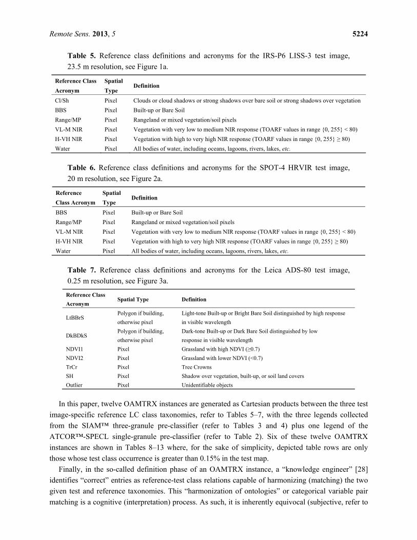
Table 5. Reference class definitions and acronyms for the IRS-P6 LISS-3 test image,
23.5 m resolution, see Figure 1a.
Reference Class
Acronym
Spatial
Type Definition
Cl/Sh Pixel Clouds or cloud shadows or strong shadows over bare soil or strong shadows over vegetation
BBS Pixel Built-up or Bare Soil
Range/MP Pixel Rangeland or mixed vegetation/soil pixels
VL-M NIR Pixel Vegetation with very low to medium NIR response (TOARF values in range {0, 255} < 80)
H-VH NIR Pixel Vegetation with high to very high NIR response (TOARF values in range {0, 255} ≥ 80)
Water Pixel All bodies of water, including oceans, lagoons, rivers, lakes, etc.
Table 6. Reference class definitions and acronyms for the SPOT-4 HRVIR test image,
20 m resolution, see Figure 2a.
Reference
Class Acronym
Spatial
Type Definition
BBS Pixel Built-up or Bare Soil
Range/MP Pixel Rangeland or mixed vegetation/soil pixels
VL-M NIR Pixel Vegetation with very low to medium NIR response (TOARF values in range {0, 255} < 80)
H-VH NIR Pixel Vegetation with high to very high NIR response (TOARF values in range {0, 255} ≥ 80)
Water Pixel All bodies of water, including oceans, lagoons, rivers, lakes, etc.
Table 7. Reference class definitions and acronyms for the Leica ADS-80 test image,
0.25 m resolution, see Figure 3a.
Reference Class
Acronym Spatial Type Definition
LtBBrS Polygon if building,
otherwise pixel
Light-tone Built-up or Bright Bare Soil distinguished by high response
in visible wavelength
DkBDkS Polygon if building,
otherwise pixel
Dark-tone Built-up or Dark Bare Soil distinguished by low
response in visible wavelength
NDVI1 Pixel Grassland with high NDVI (≥0.7)
NDVI2 Pixel Grassland with lower NDVI (<0.7)
TrCr Pixel Tree Crowns
SH Pixel Shadow over vegetation, built-up, or soil land covers
Outlier Pixel Unidentifiable objects
In this paper, twelve OAMTRX instances are generated as Cartesian products between the three test
image-specific reference LC class taxonomies, refer to Tables 5–7, with the three legends collected
from the SIAM™ three-granule pre-classifier (refer to Tables 3 and 4) plus one legend of the
ATCOR™-SPECL single-granule pre-classifier (refer to Table 2). Six of these twelve OAMTRX
instances are shown in Tables 8–13 where, for the sake of simplicity, depicted table rows are only
those whose test class occurrence is greater than 0.15% in the test map.
Finally, in the so-called definition phase of an OAMTRX instance, a “knowledge engineer” [28]
identifies “correct” entries as reference-test class relations capable of harmonizing (matching) the two
given test and reference taxonomies. This “harmonization of ontologies” or categorical variable pair
matching is a cognitive (interpretation) process. As such, it is inherently equivocal (subjective, refer to
Remote Sens. 2013, 5 5225
the Part 1, Section 2.1 [20]). This means that, in general, categorical variable pair matching requires
negotiation and to be community-agreed upon [38,39,42–44,46]. Notably, the categorical variable pair
matching phase is independent of the OAMTRX instantiation with probability values. In common
practice, the former predates the latter (also refer to the introduction to Section 3).
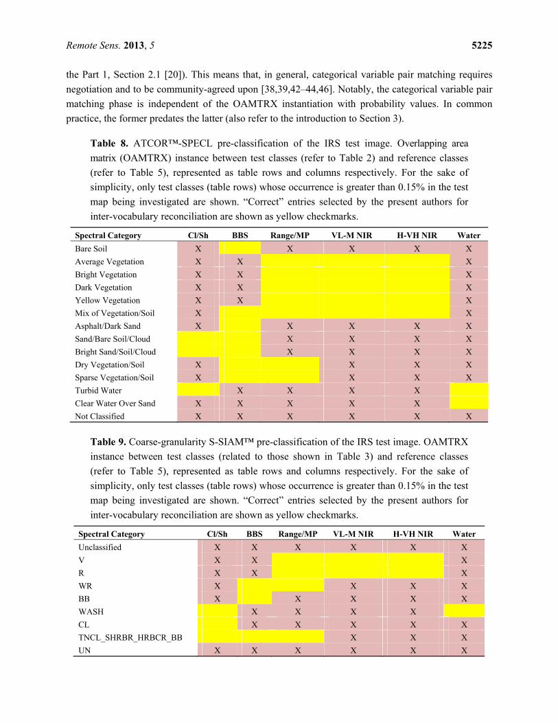
Table 8. ATCOR™-SPECL pre-classification of the IRS test image. Overlapping area
matrix (OAMTRX) instance between test classes (refer to Table 2) and reference classes
(refer to Table 5), represented as table rows and columns respectively. For the sake of
simplicity, only test classes (table rows) whose occurrence is greater than 0.15% in the test
map being investigated are shown. “Correct” entries selected by the present authors for
inter-vocabulary reconciliation are shown as yellow checkmarks.
Spectral Category Cl/Sh BBS Range/MP VL-M NIR H-VH NIR Water
Bare Soil X � X X X X
Average Vegetation X X � � � X
Bright Vegetation X X � � � X
Dark Vegetation X X � � � X
Yellow Vegetation X X � � � X
Mix of Vegetation/Soil X � � � � X
Asphalt/Dark Sand X � X X X X
Sand/Bare Soil/Cloud � � X X X X
Bright Sand/Soil/Cloud � � X X X X
Dry Vegetation/Soil X � � X X X
Sparse Vegetation/Soil X � � X X X
Turbid Water � X X X X �
Clear Water Over Sand X X X X X �
Not Classified X X X X X X
Table 9. Coarse-granularity S-SIAM™ pre-classification of the IRS test image. OAMTRX
instance between test classes (related to those shown in Table 3) and reference classes
(refer to Table 5), represented as table rows and columns respectively. For the sake of
simplicity, only test classes (table rows) whose occurrence is greater than 0.15% in the test
map being investigated are shown. “Correct” entries selected by the present authors for
inter-vocabulary reconciliation are shown as yellow checkmarks.
Spectral Category Cl/Sh BBS Range/MP VL-M NIR H-VH NIR Water
Unclassified X X X X X X
V X X � � � X
R X X � � � X
WR X � � X X X
BB X � X X X X
WASH � X X X X �
CL � X X X X X
TNCL_SHRBR_HRBCR_BB � � � X X X
UN X X X X X X
Remote Sens. 2013, 5 5226
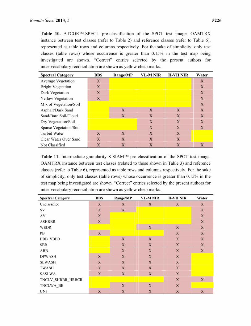
Table 10. ATCOR™-SPECL pre-classification of the SPOT test image. OAMTRX
instance between test classes (refer to Table 2) and reference classes (refer to Table 6),
represented as table rows and columns respectively. For the sake of simplicity, only test
classes (table rows) whose occurrence is greater than 0.15% in the test map being
investigated are shown. “Correct” entries selected by the present authors for
inter-vocabulary reconciliation are shown as yellow checkmarks.
Spectral Category BBS Range/MP VL-M NIR H-VH NIR Water
Average Vegetation X � � � X Bright Vegetation X � � � X Dark Vegetation X � � � X Yellow Vegetation X � � � X Mix of Vegetation/Soil � � � � X Asphalt/Dark Sand � X X X X Sand/Bare Soil/Cloud � X X X X Dry Vegetation/Soil � � X X X Sparse Vegetation/Soil � � X X X Turbid Water X X X X � Clear Water Over Sand X X X X � Not Classified X X X X X
Table 11. Intermediate-granularity S-SIAM™ pre-classification of the SPOT test image.
OAMTRX instance between test classes (related to those shown in Table 3) and reference
classes (refer to Table 6), represented as table rows and columns respectively. For the sake
of simplicity, only test classes (table rows) whose occurrence is greater than 0.15% in the
test map being investigated are shown. “Correct” entries selected by the present authors for
inter-vocabulary reconciliation are shown as yellow checkmarks.
Spectral Category BBS Range/MP VL-M NIR H-VH NIR Water
Unclassified X X X X X
SV X X � � X
AV X � � � X
ASHRBR X � � � X
WEDR � � X X X
PB X � � X X
BBB_VBBB � X X X X
SBB � X X X X
ABB � X X X X
DPWASH X X X X �
SLWASH X X X X �
TWASH X X X X �
SASLWA X X X X �
TNCLV_SHRBR_HRBCR � � � X X
TNCLWA_BB � X X X �
UN3 X X X X X
Remote Sens. 2013, 5 5227
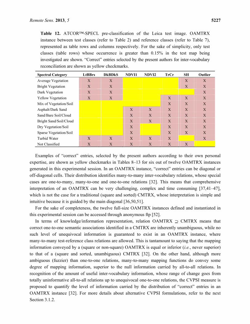
Table 12. ATCOR™-SPECL pre-classification of the Leica test image. OAMTRX
instance between test classes (refer to Table 2) and reference classes (refer to Table 7),
represented as table rows and columns respectively. For the sake of simplicity, only test
classes (table rows) whose occurrence is greater than 0.15% in the test map being
investigated are shown. “Correct” entries selected by the present authors for inter-vocabulary
reconciliation are shown as yellow checkmarks.
Spectral Category LtBBrs DkBDkS NDVI1 NDVI2 TrCr SH Outlier
Average Vegetation X X � � � X X
Bright Vegetation X X � � � X X
Dark Vegetation X X � � � � X
Yellow Vegetation X X � � X X X
Mix of Vegetation/Soil � � � � X X X
Asphalt/Dark Sand � � X X X X X
Sand/Bare Soil/Cloud � � X X X X X
Bright Sand/Soil/Cloud � � X X X X X
Dry Vegetation/Soil � � X � X X X
Sparse Vegetation/Soil � � X � X X X
Turbid Water X X X X X � X
Not Classified X X X X X X �
Examples of “correct” entries, selected by the present authors according to their own personal
expertise, are shown as yellow checkmarks in Tables 8–13 for six out of twelve OAMTRX instances
generated in this experimental session. In an OAMTRX instance, “correct” entries can be diagonal or
off-diagonal cells. Their distribution identifies many-to-many inter-vocabulary relations, whose special
cases are one-to-many, many-to-one and one-to-one relations [32]. This means that comprehensive
interpretation of an OAMTRX can be very challenging, complex and time consuming [37,41–47],
which is not the case for a traditional (square and sorted) CMTRX, whose interpretation is simple and
intuitive because it is guided by the main diagonal [36,50,51].
For the sake of completeness, the twelve full-size OAMTRX instances defined and instantiated in
this experimental session can be accessed through anonymous ftp [52].
In terms of knowledge/information representation, relation OAMTRX ⊇ CMTRX means that
correct one-to-one semantic associations identified in a CMTRX are inherently unambiguous, while no
such level of unequivocal information is guaranteed to exist in an OAMTRX instance, where
many-to-many test-reference class relations are allowed. This is tantamount to saying that the mapping
information conveyed by a (square or non-square) OAMTRX is equal or inferior (i.e., never superior)
to that of a (square and sorted, unambiguous) CMTRX [32]. On the other hand, although more
ambiguous (fuzzier) than one-to-one relations, many-to-many mapping functions do convey some
degree of mapping information, superior to the null information carried by all-to-all relations. In
recognition of the amount of useful inter-vocabulary information, whose range of change goes from
totally uninformative all-to-all relations up to unequivocal one-to-one relations, the CVPSI measure is
proposed to quantify the level of information carried by the distribution of “correct” entries in an
OAMTRX instance [32]. For more details about alternative CVPSI formulations, refer to the next
Section 3.1.2.
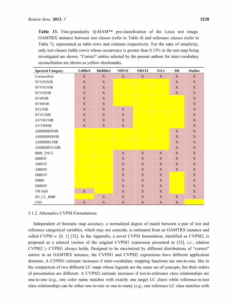
Remote Sens. 2013, 5 5228
Table 13. Fine-granularity Q-SIAM™ pre-classification of the Leica test image.
OAMTRX instance between test classes (refer to Table 4) and reference classes (refer to
Table 7), represented as table rows and columns respectively. For the sake of simplicity,
only test classes (table rows) whose occurrence is greater than 0.15% in the test map being
investigated are shown. “Correct” entries selected by the present authors for inter-vocabulary
reconciliation are shown as yellow checkmarks.
Spectral Category LtBBrS DkBDkS NDVI1 NDVI2 TrCr SH Outlier
Unclassified X X X X X X X
SVVH2NIR X X � � � X X
SVVH1NIR X X � � � X X
SVVHNIR X X � � � X X
SVHNIR X X � � � � X
SVMNIR X X � � � � X
SVLNIR X X X � � � X
SVVLNIR X X X � � � X
AVVH1NIR X X X � � � X
AVVHNIR X X X � � � X
ASHRBRHNIR � � � � � X X
ASHRBRMNIR � � � � � X X
ASHRBRLNIR � � � � � X X
ASHRBRVLNIR � � � � � X X
BBB_TNCL � � X X X X X
SBBNF � � X X X X X
ABBVF � � X X X X X
ABBNF � � X X X X X
DBBVF � � X X X � X
DBBF � � X X X � X
DBBNF � � X X X � X
TWASH X � X X X � X
SN_CL_BBB � X X X X X X
UN3 X X X X X X �
3.1.2. Alternative CVPSI Formulations
Independent of thematic map accuracy, a normalized degree of match between a pair of test and
reference categorical variables, which may not coincide, is estimated from an OAMTRX instance and
called CVPSI ∈ [0, 1] [32]. In the Appendix, a novel CVPSI formulation, identified as CVPSI2, is
proposed as a relaxed version of the original CVPSI1 expression presented in [32], i.e., relation
CVPSI2 ≥ CVPSI1 always holds. Designed to be maximized by different distributions of “correct”
entries in an OAMTRX instance, the CVPSI1 and CVPSI2 expressions have different application
domains. A CVPSI1 estimate increases if inter-vocabulary mapping functions are one-to-one, like in
the comparison of two different LC maps whose legends are the same set of concepts, but their orders
of presentation are different. A CVPSI2 estimate increases if test-to-reference class relationships are
one-to-one (e.g., one color name matches with exactly one target LC class) while reference-to-test
class relationships can be either one-to-one or one-to-many (e.g., one reference LC class matches with
Remote Sens. 2013, 5 5229
at least one or more color names). Notably, between the two CVPSI1 and CVPSI2 formulations, the
latter is the one suitable for best modeling the mapping problem at hand, from reference LC classes to
test spectral categories and vice versa, refer to the Appendix.
Hereafter, the acronym CVPSI is used to mean the ensemble of CVPSI1 and CVPSI2 values.
Notably, variable (1 − CVPSI) ∈ [0, 1], complementary to CVPSI, can be interpreted as a
normalized estimate of the mapping (classification) effort required to fill up the residual semantic gap
from the test to the reference pair of semantic vocabularies. For example, if CVPSI = 0.4 at the
pre-attentive vision first stage of a two-stage RS-IUS, then (1 − CVPSI) = 0.6 is the residual semantic
gap from test to reference vocabularies to be filled up by the attentive vision second stage, refer to the
Part 1, Figure 1c [20].
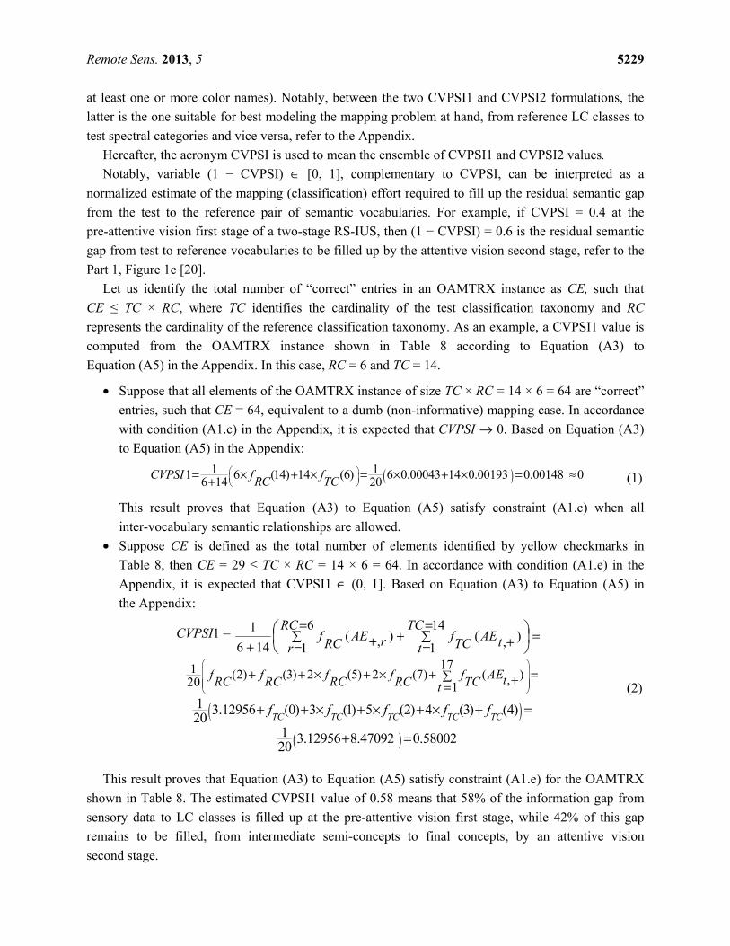
Let us identify the total number of “correct” entries in an OAMTRX instance as CE, such that
CE ≤ TC × RC, where TC identifies the cardinality of the test classification taxonomy and RC
represents the cardinality of the reference classification taxonomy. As an example, a CVPSI1 value is
computed from the OAMTRX instance shown in Table 8 according to Equation (A3) to
Equation (A5) in the Appendix. In this case, RC = 6 and TC = 14.
• Suppose that all elements of the OAMTRX instance of size TC × RC = 14 × 6 = 64 are “correct”
entries, such that CE = 64, equivalent to a dumb (non-informative) mapping case. In accordance
with condition (A1.c) in the Appendix, it is expected that CVPSI → 0. Based on Equation (A3)
to Equation (A5) in the Appendix:
( )1 11 6 (14) 14 (6) 6 0.00043 14 0.00193 0.00148 06 14 20
CVPSI f fRC TC
= × + × = × + × = ≈+
(1)
This result proves that Equation (A3) to Equation (A5) satisfy constraint (A1.c) when all
inter-vocabulary semantic relationships are allowed.
• Suppose CE is defined as the total number of elements identified by yellow checkmarks in
Table 8, then CE = 29 ≤ TC × RC = 14 × 6 = 64. In accordance with condition (A1.e) in the
Appendix, it is expected that CVPSI1 ∈ (0, 1]. Based on Equation (A3) to Equation (A5) in
the Appendix:
CVPSI1 = ==
= ++=
= ++
14
1),(
6
1),(
146
1 TC
t tAETC
fRC
r rAERC
f
171 (2) (3) 2 (5) 2 (7) ( ),20 1f f f f f AEtRC RC RC RC TCt
+ + × + × + = +=
( )1 3.12956 (0) 3 (1) 5 (2) 4 (3) (4)20 TC TC TC TC TC
f f f f f+ + × + × + × + =
( )1 3.12956 8.47092 0.5800220
+ =
(2)
This result proves that Equation (A3) to Equation (A5) satisfy constraint (A1.e) for the OAMTRX
shown in Table 8. The estimated CVPSI1 value of 0.58 means that 58% of the information gap from
sensory data to LC classes is filled up at the pre-attentive vision first stage, while 42% of this gap
remains to be filled, from intermediate semi-concepts to final concepts, by an attentive vision
second stage.
Remote Sens. 2013, 5 5230
In general, for a given reference vocabulary (say, a reference set of apple types: “apple_1”,
“apple_2”, etc.), it is unreasonable to expect the CVPSI value to monotonically increase with the
cardinality of the test set of concepts (say, a test set of orange types: “orange_1”, “orange_2”, etc.),
irrespective of the semantic matching between the two vocabularies. For example, the CVPSI value
between reference apples and test oranges is zero irrespective of the cardinality of the test set of
oranges. In particular cases, when the two test and reference vocabularies are semantically “consistent”
(say, a reference set of apple types: “apple_1”, “apple_2”, etc., and a single test class called “fruits”), a
finer semantic granularity of the test vocabulary or reference vocabulary or both causes the
CVPSI to increase or remain the same (never decrease), meaning that the inter-vocabulary mapping
becomes less ambiguous, like a quantization error is monotonically non-increasing with the number of
quantization levels.
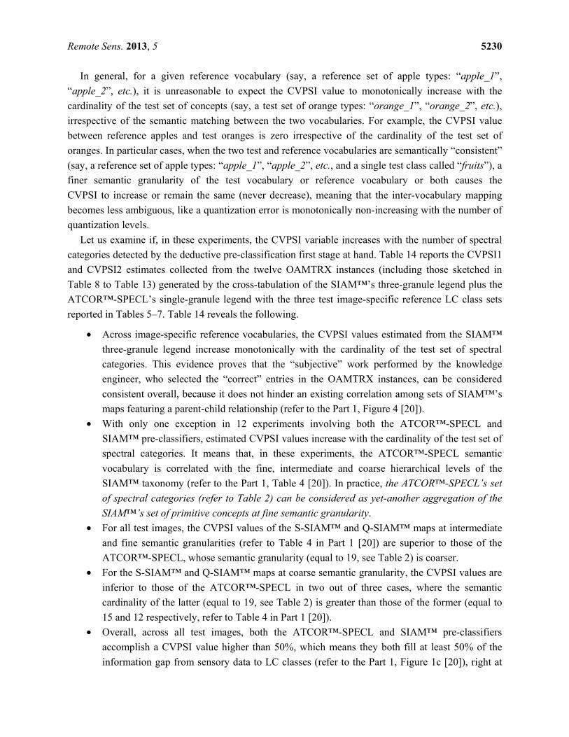
Let us examine if, in these experiments, the CVPSI variable increases with the number of spectral
categories detected by the deductive pre-classification first stage at hand. Table 14 reports the CVPSI1
and CVPSI2 estimates collected from the twelve OAMTRX instances (including those sketched in
Table 8 to Table 13) generated by the cross-tabulation of the SIAM™’s three-granule legend plus the
ATCOR™-SPECL’s single-granule legend with the three test image-specific reference LC class sets
reported in Tables 5–7. Table 14 reveals the following.
• Across image-specific reference vocabularies, the CVPSI values estimated from the SIAM™
three-granule legend increase monotonically with the cardinality of the test set of spectral
categories. This evidence proves that the “subjective” work performed by the knowledge
engineer, who selected the “correct” entries in the OAMTRX instances, can be considered
consistent overall, because it does not hinder an existing correlation among sets of SIAM™’s
maps featuring a parent-child relationship (refer to the Part 1, Figure 4 [20]).
• With only one exception in 12 experiments involving both the ATCOR™-SPECL and
SIAM™ pre-classifiers, estimated CVPSI values increase with the cardinality of the test set of
spectral categories. It means that, in these experiments, the ATCOR™-SPECL semantic
vocabulary is correlated with the fine, intermediate and coarse hierarchical levels of the
SIAM™ taxonomy (refer to the Part 1, Table 4 [20]). In practice, the ATCOR™-SPECL’s set
of spectral categories (refer to Table 2) can be considered as yet-another aggregation of the
SIAM™’s set of primitive concepts at fine semantic granularity.
• For all test images, the CVPSI values of the S-SIAM™ and Q-SIAM™ maps at intermediate
and fine semantic granularities (refer to Table 4 in Part 1 [20]) are superior to those of the
ATCOR™-SPECL, whose semantic granularity (equal to 19, see Table 2) is coarser.
• For the S-SIAM™ and Q-SIAM™ maps at coarse semantic granularity, the CVPSI values are
inferior to those of the ATCOR™-SPECL in two out of three cases, where the semantic
cardinality of the latter (equal to 19, see Table 2) is greater than those of the former (equal to
15 and 12 respectively, refer to Table 4 in Part 1 [20]).
• Overall, across all test images, both the ATCOR™-SPECL and SIAM™ pre-classifiers
accomplish a CVPSI value higher than 50%, which means they both fill at least 50% of the
information gap from sensory data to LC classes (refer to the Part 1, Figure 1c [20]), right at
Remote Sens. 2013, 5 5231
the pre-attentive vision first stage, without user interactions and in near real-time, which
means at no cost in manpower and computer power.
To recapitulate, in these experiments, where the semantic degree of match between spectral
categories and target LC classes is estimated as a scalar value, CVPSI ∈ [0, 1], independent of the
mapping accuracy indexes, TQIs and SQIs (refer to the farther Section 3.4.1), conclusions are
the following.
1. The SIAM™ multi-granule pre-classifier appears more effective than the ATCOR™-SPECL
single-granule pre-classifier in filling up the information gap from sensory data to LC classes
(refer to the Part 1, Section 2.3 and Figure 1c [20]).
2. Approximately 50% of the information gap from sensory data to LC classes is filled by the
SIAM™ pre-classification first stage and accomplished without user’s supervision and in near
real-time. To be considered of potential interest, in addition to being informative because its
CVPSI value scores high, the SIAM™ pre-classification first stage must also be accurate, i.e.,
its TQIs and SQIs must score high simultaneously with the CVPSI.
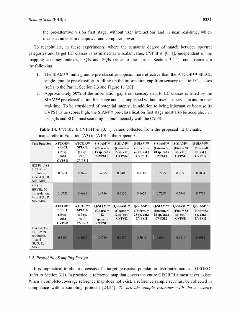
Table 14. CVPSI2 ≥ CVPSI1 ∈ [0, 1] values collected from the proposed 12 thematic
maps, refer to Equation (A3) to (A10) in the Appendix.
Test Data Set ATCOR™ SPECL
(19 sp. cat.)
CVPSI1
ATCOR™ SPECL
(19 sp. cat.)
CVPSI2
S-SIAM™
(Coarse = 15 sp. cat.)
CVPSI1
S-SIAM™
(Coarse = 15 sp. cat.)
CVPSI2
S-SIAM™
(Interm. = 40 sp. cat.)
CVPSI1
S-SIAM™
(Interm. = 40 sp. cat.)
CVPSI2
S-SIAM™
(Fine = 68 sp. cat.) CVPSI1
S-SIAM™
(Fine = 68 sp. cat.) CVPSI2
IRS-P6 LISS-3, 23.5 m-resolution, 4-band (G, R, NIR, MIR)
0.6631 0.7696 0.4855 0.6480 0.7110 0.7755 0.7653 0.8034
SPOT-4 HRVIR, 20 m-resolution, 4-band (G, R, NIR, MIR)
0. 5732 0.6688 0.4746 0.6135 0.6659 0.7208 0.7449 0.7796
ATCOR™ SPECL
(19 sp. cat.)
CVPSI1
ATCOR™ SPECL
(19 sp. cat.)
CVPSI2
Q-SIAM™
(Coarse = 12
sp. cat.) CVPSI1
Q-SIAM™
(Coarse = 12 sp. cat.)
CVPSI2
Q-SIAM™
(Interm. = 28 sp. cat.)
CVPSI1
Q-SIAM™
(Interm. = 28 sp. cat.)
CVPSI2
Q-SIAM™
(Fine = 52 sp. cat.) CVPSI1
Q-SIAM™
(Fine = 52 sp. cat.) CVPSI2
Leica ADS-40, 0.25 m-resolution, 4-band (B, G, R, NIR)
0.5000 0.6073 0.4249 0.6337 0.5642 0.6664 0.6310 0.6911
3.2. Probability Sampling Design
It is impractical to obtain a census of a target geospatial population distributed across a GEOROI
(refer to Section 3.1). In practice, a reference map that covers the entire GEOROI almost never exists.
When a complete-coverage reference map does not exist, a reference sample set must be collected in
compliance with a sampling protocol [24,25]. To provide sample estimates with the necessary

Remote Sens. 2013, 5 5232
probability foundation to permit generalization from the sample data set to the target geospatial
population, probability sampling design and implementation become mandatory under constraints
discussed in Part 1, Section 2.6 [20]. Probability sampling design consists of the following steps.
(i) Estimation of the sample set cardinality depending on the project’s requirements specification.
(ii) Selection of the sampling frame. (iii) Selection of the spatial type(s) of sampling units.
(iv) Selection of the sampling strategy. These steps are developed below.
3.2.1. Reference Sample Set Cardinality and Degree of Uncertainty in Measurement
Statistical functions that link the sample overall accuracy of a thematic map with the sample degree
of tolerance and the reference sample set size are selected from the existing literature. Next, a
minimum reference sample cardinality is estimated as a function of the target overall accuracy and
error tolerance listed in the project requirements specification.
Statistical Level of Confidence and Level of Significance of a Sample overall Accuracy
In order to estimate the minimum number of reference sampling units to be sampled and labeled for
each reference class, Lunetta and Elvidge propose a statistical criterion which depends on the project
requirements specification, namely, the target class-specific accuracy and error tolerance, but is
independent of costs of sampling to be accounted for in the project budget [50]. This statistical
criterion is described below.
An overall accuracy (OA) measure is represented by a probability accuracy estimate (a random
variable), , and its associated confidence interval (an error tolerance), ± . Furthermore, the
half-width of the error tolerance, , exists at a specified confidence level ( 1−∝ ) such that 0 < < ≤ 1 with ∝∈ [0,1]. The desired level of significance, represented by ∝, defines the risk
that the actual error is larger than ± .
Assuming that reference samples are independent and identically distributed (i.i.d.; notably, the
i.i.d. property is almost always violated in the RS common practice, due to spatial autocorrelation
within neighboring pixels of the same LC type), the half-width of the error tolerance, , can be
computed based upon the desired accuracy estimate, confidence level, and sample set size ( )
according to [50]:
= χ( , ∝) ∙ ∙ (1 − ) (3)
where χ( , ∝) is the upper (1– α) × 100th percentile of the chi-square distribution with one degree of
freedom, e.g., if the level of confidence is (1 − 0.01) = 0.99, then ( , . ) . . It follows that the
necessary reference dataset size, , may be estimated as
For the purpose of assessment of individual classes involved in the classification process, for each
c-th class with c=1, … , C, where C is the total number of classes, it is possible to prove that [50]
= χ( , ∝) ∙ ∙ (1 − ) (4)
Remote Sens. 2013, 5 5233
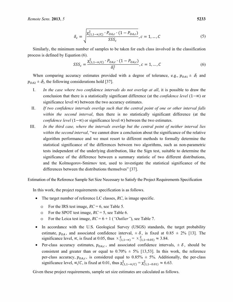
Similarly, the minimum number of samples to be taken for each class involved in the classification
process is defined by Equation (6).
When comparing accuracy estimates provided with a degree of tolerance, e.g., ± δ1 and
± δ2, the following considerations hold [37].
I. In the case where two confidence intervals do not overlap at all, it is possible to draw the
conclusion that there is a statistically significant difference (at the confidence level (1−∝) or
significance level ∝) between the two accuracy estimates.
II. If two confidence intervals overlap such that the central point of one or other interval falls
within the second interval, then there is no statistically significant difference (at the
confidence level (1−∝) or significance level ∝) between the two estimates.
III. In the third case, where the intervals overlap but the central point of neither interval lies
within the second interval, “we cannot draw a conclusion about the significance of the relative
algorithm performance and we must resort to different methods to formally determine the
statistical significance of the differences between two algorithms, such as non-parametric
tests independent of the underlying distribution, like the Sign test, suitable to determine the
significance of the difference between a summary statistic of two different distributions,
and the Kolmogorov-Smirnov test, used to investigate the statistical significance of the
differences between the distributions themselves” [37].
Estimation of the Reference Sample Set Size Necessary to Satisfy the Project Requirements Specification
In this work, the project requirements specification is as follows.
• The target number of reference LC classes, RC, is image specific.
o For the IRS test image, RC = 6, see Table 5.
o For the SPOT test image, RC = 5, see Table 6.
o For the Leica test image, RC = 6 + 1 (“Outlier”), see Table 7.
• In accordance with the U.S. Geological Survey (USGS) standards, the target probability
estimate, , and associated confidence interval, ± , is fixed at 0.85 ± 2% [13]. The significance level, ∝, is fixed at 0.05, thus χ( , ∝) = χ( , . ) ≈ 3.84.
• Per-class accuracy estimates, , , and associated confidence intervals, ± , should be
consistent and greater than or equal to 0.70% ± 5% [13,53]. In this work, the reference per-class accuracy, , , is considered equal to 0.85% ± 5%. Additionally, the per-class significance level, ∝/ , is fixed at 0.01, thus χ( , ∝/ ) = χ( , . ) ≈ 6.63.
Given these project requirements, sample set size estimates are calculated as follows.
= χ( , ∝/ ) ∙ , ∙ (1 − , ) , = 1, … , (5)
= χ( , ∝/ ) ∙ , ∙ (1 − , ) , = 1,… , (6)
Remote Sens. 2013, 5 5234
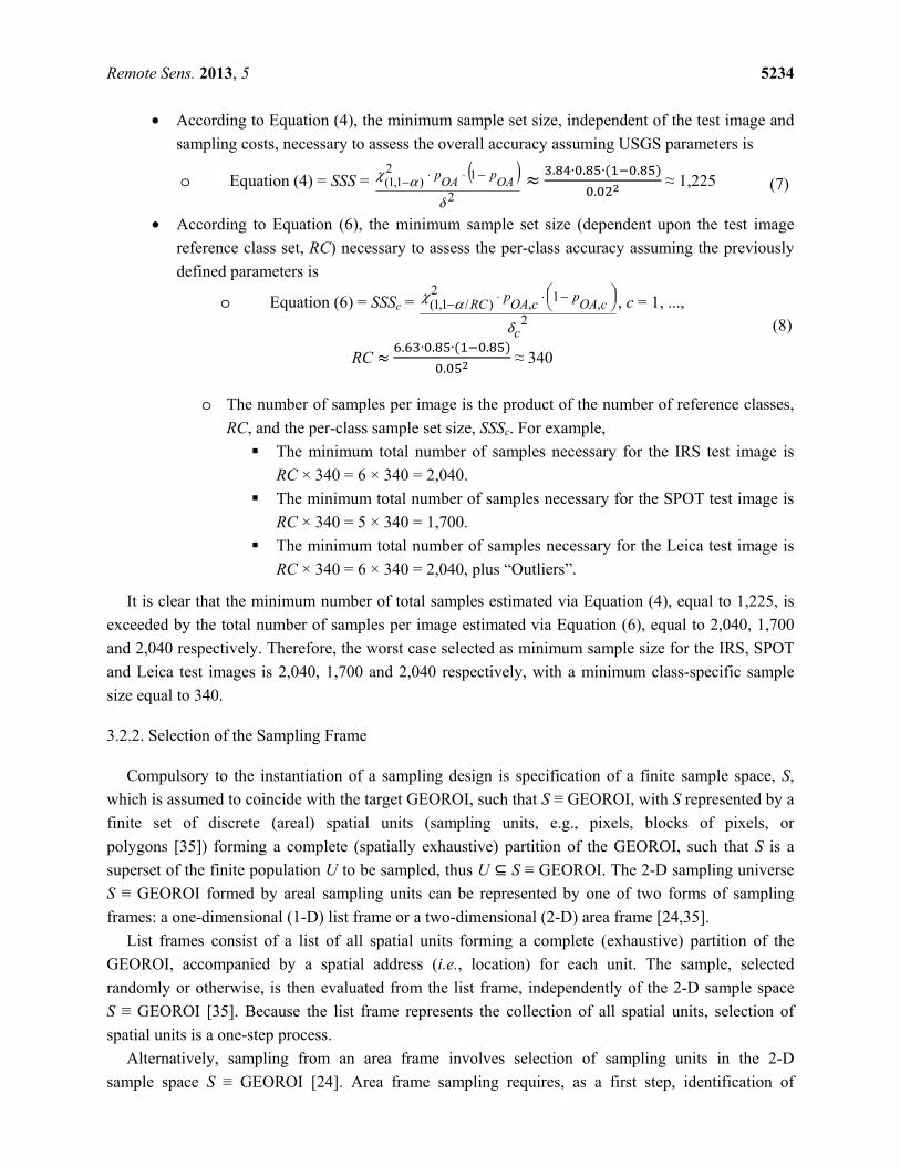
• According to Equation (4), the minimum sample set size, independent of the test image and
sampling costs, necessary to assess the overall accuracy assuming USGS parameters is
o Equation (4) = SSS = ( )2
12)1,1(
δαχ
OAp
OAp −⋅⋅− ≈
. ∙ . ∙( . ). ≈ 1,225 (7)
• According to Equation (6), the minimum sample set size (dependent upon the test image
reference class set, RC) necessary to assess the per-class accuracy assuming the previously
defined parameters is
o Equation (6) = SSSc = 2
,1
,2
)/1,1(
c
cOAp
cOAp
RC
δ
αχ
−⋅⋅− , c = 1, ...,
RC ≈ . ∙ . ∙( . ). ≈ 340
(8)
o The number of samples per image is the product of the number of reference classes,
RC, and the per-class sample set size, SSSc. For example,
The minimum total number of samples necessary for the IRS test image is
RC × 340 = 6 × 340 = 2,040.
The minimum total number of samples necessary for the SPOT test image is
RC × 340 = 5 × 340 = 1,700.
The minimum total number of samples necessary for the Leica test image is
RC × 340 = 6 × 340 = 2,040, plus “Outliers”.
It is clear that the minimum number of total samples estimated via Equation (4), equal to 1,225, is
exceeded by the total number of samples per image estimated via Equation (6), equal to 2,040, 1,700
and 2,040 respectively. Therefore, the worst case selected as minimum sample size for the IRS, SPOT
and Leica test images is 2,040, 1,700 and 2,040 respectively, with a minimum class-specific sample
size equal to 340.
3.2.2. Selection of the Sampling Frame
Compulsory to the instantiation of a sampling design is specification of a finite sample space, S,
which is assumed to coincide with the target GEOROI, such that S ≡ GEOROI, with S represented by a
finite set of discrete (areal) spatial units (sampling units, e.g., pixels, blocks of pixels, or
polygons [35]) forming a complete (spatially exhaustive) partition of the GEOROI, such that S is a
superset of the finite population U to be sampled, thus U ⊆ S ≡ GEOROI. The 2-D sampling universe
S ≡ GEOROI formed by areal sampling units can be represented by one of two forms of sampling
frames: a one-dimensional (1-D) list frame or a two-dimensional (2-D) area frame [24,35].
List frames consist of a list of all spatial units forming a complete (exhaustive) partition of the
GEOROI, accompanied by a spatial address (i.e., location) for each unit. The sample, selected
randomly or otherwise, is then evaluated from the list frame, independently of the 2-D sample space
S ≡ GEOROI [35]. Because the list frame represents the collection of all spatial units, selection of
spatial units is a one-step process.
Alternatively, sampling from an area frame involves selection of sampling units in the 2-D
sample space S ≡ GEOROI [24]. Area frame sampling requires, as a first step, identification of

Remote Sens. 2013, 5 5235
dimensionless spatial locations (also called sample candidates or sample locations [24]), otherwise
termed geo-atoms [45], equivalent to a dimensionless atomic abstraction of geographic information.
An explicit rule for associating a unique sampling unit, say, either a pixel, polygon or block of pixels,
with any spatial location within the area frame must be established. For example, a rule for associating
a unique polygon with a randomly selected point location is to sample that polygon within which the
random point fell. This particular area frame sampling strategy illustrates that it is not necessary to
delineate all polygons in the target population to obtain the sample, like in a list-frame sampling.
Furthermore, area frames better retain the 2-D spatial structure important for systematic sampling of a
geospatial population [24].
In this work, where no complete coverage reference maps are available for the test maps, no list
frame can be adopted for sampling. Rather, an area frame is employed for sampling.
3.2.3. Selection of the Spatial Types of Sampling Units
The (areal) sampling unit represents the 2-D unit of the GEOROI upon which accuracy assessment
is carried out. The sampling unit can be defined without specifying what will be observed on that unit
on the ground; thus no assumption about homogeneity of thematic classes for the sampling unit is
necessary [32]. For any type of sampling unit, there are multiple acceptable sampling and response
designs. It is therefore necessary to clearly define the sampling unit before attempting to determine the
sampling and response designs [24]. Three basic types of areal sampling units exist [24].
• Pixels, representing small areas (e.g., 30 m pixel), are related to the dimensionless sample
location described in Section 3.2.2, but because pixels still possess some areal extent, they
partition the mapped population into a finite, though large, number of sampling units.
• Polygons, typically irregular in shape and differing in size to approximate the shape and size of
a target 3-D object, e.g., a target building.
• Fixed-area plots, generally regular in shape and area which cover a chosen areal extent
(typically a 3 × 3 or 5 × 5 pixel plot).
It should be noted that pixels and polygons are special cases of the fixed-area plot spatial unit type.
In the present paper, pixel units are adopted to represent all samples used by the TQI estimators
(refer to the farther Section 3.4.1) while polygons are necessary for SQI estimators of reference
image-objects (segments) whose shape is salient for detection, such as single-date (2-D) image-objects
depicting man-made 4-D objects in the world-through-time, like “buildings” and “roads” (refer
to the farther Section 3.4.1). Notably, image-objects depicting single instances of man-made
objects-through-time (e.g., buildings, roads, etc.) are visible only in the VHR Leica image, see
Figure 3 and refer to Tables 5–7. It means that segment-based SQIs can be estimated only from the
Leica test image.
3.2.4. Selection of the Sampling Strategy
Simple random sampling (SIRS), stratified random sampling (consisting of a SIRS of elements
from the elements in stratum ℎ), systematic sampling (with a random start and sampling interval K,
where K is an integer), and cluster sampling are all probability sampling designs considered as
Remote Sens. 2013, 5 5236
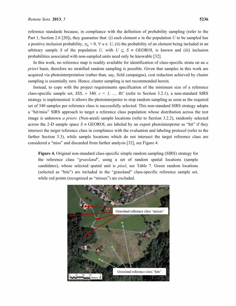
reference standards because, in compliance with the definition of probability sampling (refer to the
Part 1, Section 2.6 [20]), they guarantee that: (i) each element u in the population U to be sampled has
a positive inclusion probability, > 0, ∀ u ∈ U, (ii) the probability of an element being included in an
arbitrary sample S of the population U, with U ⊆ S ≡ GEOROI, is known and (iii) inclusion
probabilities associated with non-sampled units need only be knowable [32].
In this work, no reference map is readily available for identification of class-specific strata on an a
priori basis, therefore no stratified random sampling is possible. Given that samples in this work are
acquired via photointerpretation (rather than, say, field campaigns), cost reduction achieved by cluster
sampling is essentially zero. Hence, cluster sampling is not recommended herein.
Instead, to cope with the project requirements specification of the minimum size of a reference
class-specific sample set, SSSc ≈ 340, c = 1, ..., RC (refer to Section 3.2.1), a non-standard SIRS
strategy is implemented: it allows the photointerpreter to stop random sampling as soon as the required
set of 340 samples per reference class is successfully selected. This non-standard SIRS strategy adopts
a “hit/miss” SIRS approach to target a reference class population whose distribution across the test
image is unknown a priori. (Non-areal) sample locations (refer to Section 3.2.2), randomly selected
across the 2-D sample space S ≡ GEOROI, are labeled by an expert photointerpreter as “hit” if they
intersect the target reference class in compliance with the evaluation and labeling protocol (refer to the
farther Section 3.3), while sample locations which do not intersect the target reference class are
considered a “miss” and discarded from further analysis [32], see Figure 4.
Figure 4. Original non-standard class-specific simple random sampling (SIRS) strategy for
the reference class “grassland”, using a set of random spatial locations (sample
candidates), whose selected spatial unit is pixel, see Table 7. Green random locations
(selected as “hits”) are included in the “grassland” class-specific reference sample set,
while red points (recognized as “misses”) are excluded.
Remote Sens. 2013, 5 5237
With regard to the polygon-based SQI assessment of the SIAM™ maps generated from the VHR
Leica image (refer to Section 3.2.3), the same “hit/miss” SIRS approach described in the previous
paragraph would normally be adopted to select instances of the reference class “buildings”, which is a
subset of the logical OR-combination of reference LC classes “Light-tone Built-up or Bright Bare
Soil” (“LtBBrS”) and “Dark-tone Built-up or Dark Bare Soil” (“DkBDkS”), whose spatial type is
polygon, refer to Table 7. However, since it is obvious that there are not enough buildings in the VHR
Leica image to reach the required cardinality of 340 instances per class (refer to Section 3.2.1), all
buildings detected by an expert photointerpreter in the Leica image are included in the sample set of
the reference class “buildings” for SQI estimation.
3.3. Response Design: Evaluation and Labeling Protocol
The purpose of response design is to assign a value or label to (areal) sampling units where
(non-areal) sample locations, selected through the sampling strategy (refer to Section 3.2.4), fell.
Response design consists of two steps: (i) the evaluation protocol and (ii) the labeling protocol [24].
The evaluation protocol comprises the means through which a spatial support region, defined as the
area where “truth” classification evidences are collected, is attached to every sampling unit where a
sample location fell [32].
A general rule of thumb would require to select the reference data source “one step closer to the
ground” than the RS data used to make up the test map [36] (refer to the introduction to Section 3).
Unfortunately, when dealing with thematic maps generated from VHR imagery, it is often the case
there is no reference data source originated: (I) at the same time of the VHR image acquisition and
(II) one step closer to the ground. For example, to assess the accuracy of thematic maps generated
from, say, the VHR Leica test image acquired in year 2007 and adopted in this work (refer to
Section 2), pre-existing VHR thematic maps dated 2007 would be required, since ground visits cannot
be performed back in time. In general, in these cases the sole data source available for reference
population sampling is the same VHR image adopted as input by the RS-IUS whose output map has to
be evaluated. In other words, the test and reference data sources coincide with the VHR image at hand.
The lack of a reference data source one step closer to the ground than the HR/VHR image at hand
should not be considered a problem, provided that the second knowledge expert (reference cognitive
agent), the one in charge of implementing the sample evaluation and labeling phases of the map
accuracy assessment protocol (refer to the farther Section 3.4), interprets the HR/VHR images by
independent means from the first (test) cognitive agent, namely, the RS-IUS whose maps are being
validated. This is to say that the reference data set should be acquired independently of the test map to
be evaluated.
In these experiments, where the spatial type of sampling units involved with TQI estimators is pixel
exclusively (refer to Section 3.2.3), the spatial support region is defined as a 2-D neighborhood,
10 × 10 pixel in size, centered on the pixel upon which the sample location fell. Similarly, the size of
the spatial support region for sampling units involved with SQI estimators, whose spatial type is
polygon, is defined as 10 times the size of the polygon belonging to the target reference class
(e.g., “buildings”) where the sample location fell.
Remote Sens. 2013, 5 5238
In series with the evaluation protocol, the labeling protocol assigns one (crisp) or more than one
(fuzzy) reference class labels to each sampling unit where a sample location fell, based on “truth”
classification evidences collected across the spatial support region centered on that sampling
unit. In these experiments, for all test images and for all selected spatial support regions, visual
evidence is collected by an expert photointerpreter to provide a crisp (“hit” or “miss”) labeling (refer to
Section 3.2.4) [32].
3.4. Analysis and Estimation Protocol
Traditional symbolic pixel-based TQIs are summary statistics of class-specific first-order
histograms [36,50], which means they are spatial context-insensitive, i.e., they are insensitive to
changes in the 2-D spatial distribution of mapping errors. In other words, symbolic pixel-based TQIs
investigate “quantification error” independently of “location error” [53,54]. On the other hand,
traditional sub-symbolic context-sensitive SQIs investigate “location error” irrespective of
“quantification error” [55]. Although highly recommended in the existing literature [53,54], location
error estimation is almost never accomplished in the RS common practice. If a location error overlook
appears justified in traditional moderate to low resolution EO image applications, where shape of
image-objects is less discernible [32,49], this lack appears unreasonable in VHR image analysis.
In this section, in compliance with the original probability sampling protocol proposed in [32],
a set of sub-symbolic polygon-based SQIs is estimated in the 2-D pre-classification map domain
independently of a set of symbolic pixel-based TQIs, estimated from an OAMTRX instance (refer to
Section 3.1).
3.4.1. Thematic Accuracy Assessment of a Classification Map
Unlike traditional TQIs of a traditional (square and sorted) CMTRX instance, whose associated
CVPSI value is trivial because always equal to 1 (refer to Section 3.1.2), TQIs estimated from an
OAMTRX instance, where (ambiguous) many-to-many reference-test class relationships are allowed,
must always be assessed and compared in combination with an OAMTRX-derived CVPSI value in
range [0, 1] (refer to Section 3.1.2). For example, if two thematic maps of the same EO image feature
the same set of TQI values, but CVPSI = 0.5 and 0.9 respectively, then the second map is to be
considered the “best” one overall, because it maximizes TQIs and the CVPSI simultaneously.
Proposed TQIs are mutually independent to cope with the non-injective property of any QI (refer to
the Part 1, Section 2.5 [20]) and are provided with a degree of uncertainty in measurement, in
accordance with the principles of statistics and the QA4EO guidelines [2].
TQI Formulations
In a relevant portion of the existing RS literature, the use of popular pixel-based TQIs estimated
from a CMTRX, such as the kappa coefficient, is strongly discouraged [51,56–58]. In line with these
recommendations, well-known pixel-based TQIs selected in this paper are the traditional overall
accuracy ( ), user’s accuracy ( ) and producer’s accuracy ( ) probabilities.
Remote Sens. 2013, 5 5239
Due to the well-known non-injective property of any QI (refer to the Part 1, Section 2.5 [20]),
alone is not sufficient to characterize thematic map accuracy, i.e., different thematic maps may feature
the same value. Since every error is an omission from the correct category and a commission to a
wrong category [36], the commission error (false positive) and the omission error (false negative),
inversely related to the and the estimators respectively, are commonly used in literature in
combination with the . All of these TQIs, namely, , and the , directly illustrate the
probability of encountering a correct or incorrect labeled pixel, i.e., they allow comparisons between
digital maps consisting of sampling units whose spatial type is pixel (refer to Section 3.2.3).
The selected pixel-based TQIs are generally expressed in terms of the (square and sorted)
CMTRX ⊆ OAMTRX, where reference classes are conventionally identified as columns [37] (refer to
Section 3.1.1). In the specific case of a CMTRX, the sum of correctly classified pixels is
equivalent to the sum of the main diagonal cells, given RC reference classes [32]:
= , (9)
User’s accuracy, , represents the conditional probability that an areal unit classified as class c,
with c = 1, …, RC, in the test map is also classified as class c in the reference sample set. Hence,
is inversely related to commission error (false positive samples). In the specialized case of a CMTRX,
is defined as follows [32,36].
, = ,∑ , = ,, (10)
Similarly, represents the conditional probability than an areal unit classified as class c, with
c = 1, …, RC, in the reference sample set is also classified as class c in the test map. Hence, is
inversely related to omission error (false negative samples). In the specialized case of a CMTRX,
is defined as follows [32,36].
, = ,∑ , = ,, (11)
As previously noted (refer to Section 3.1), a (square and sorted) CMTRX is impractical to
implement in the context of this work and is replaced by OAMTRX instances, e.g., refer to Table 8 to
Table 13. It is therefore necessary to adjust the numerators of Equations (9–11) to account for the
many-to-many relationships allowed in any OAMTRX instance. Additionally, parameter RC = TC in
Equations (10) and (11) must be split into two, namely, the cardinality of the test vocabulary, TC (e.g.,
refer to Table 14), and that of the reference vocabulary, RC, where, in general, RC ≠ TC (e.g., refer to
Tables 5–7).
Overall Accuracy Estimation
An analysis of Table 15 reveals the following.
Overall, the index scores “very high” across pre-classifiers and input data sets. This is not due
to a positive bias in the quality assessment protocol, in fact small but statistically significant
differences in accuracy between the two alternative mapping systems are detected. Rather, this overall
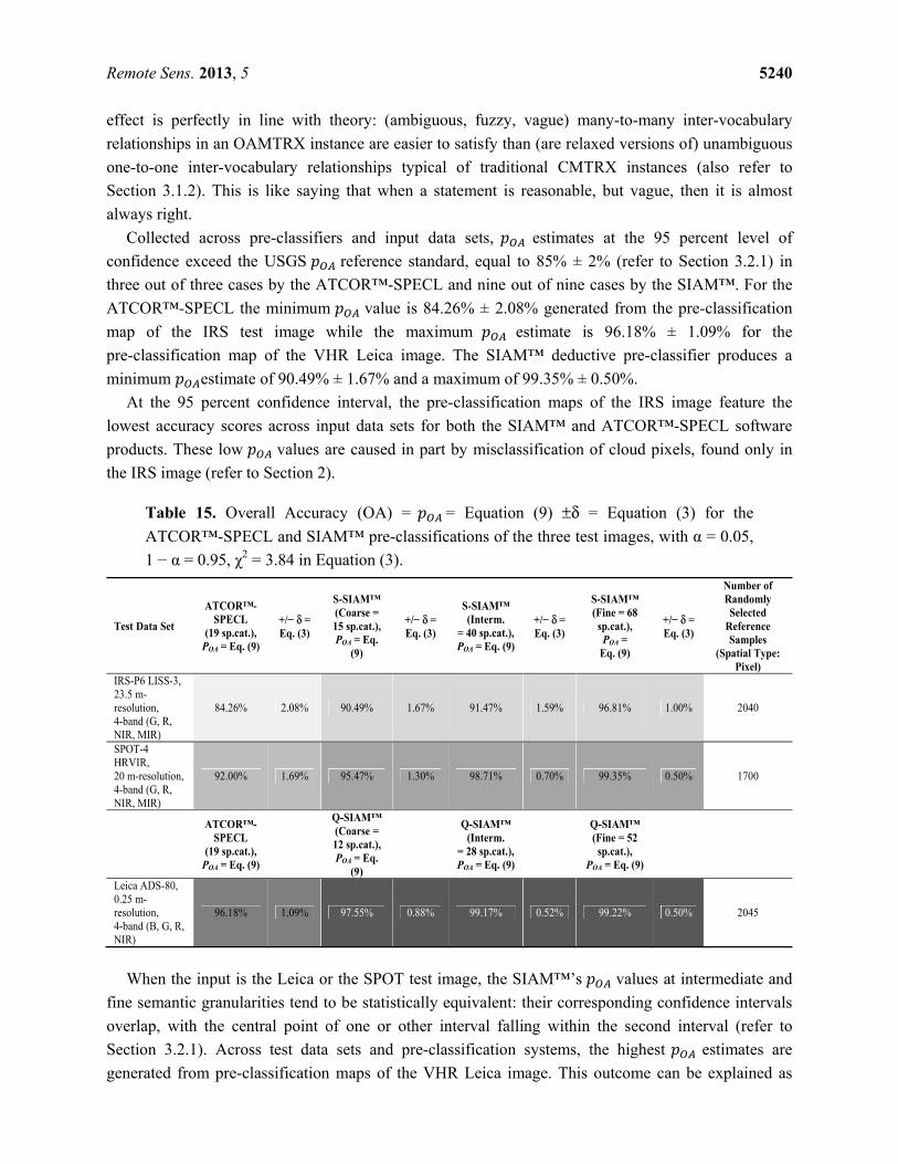
Remote Sens. 2013, 5 5240
effect is perfectly in line with theory: (ambiguous, fuzzy, vague) many-to-many inter-vocabulary
relationships in an OAMTRX instance are easier to satisfy than (are relaxed versions of) unambiguous
one-to-one inter-vocabulary relationships typical of traditional CMTRX instances (also refer to
Section 3.1.2). This is like saying that when a statement is reasonable, but vague, then it is almost
always right.
Collected across pre-classifiers and input data sets, estimates at the 95 percent level of
confidence exceed the USGS reference standard, equal to 85% ± 2% (refer to Section 3.2.1) in
three out of three cases by the ATCOR™-SPECL and nine out of nine cases by the SIAM™. For the
ATCOR™-SPECL the minimum value is 84.26% ± 2.08% generated from the pre-classification
map of the IRS test image while the maximum estimate is 96.18% ± 1.09% for the
pre-classification map of the VHR Leica image. The SIAM™ deductive pre-classifier produces a
minimum estimate of 90.49% ± 1.67% and a maximum of 99.35% ± 0.50%.
At the 95 percent confidence interval, the pre-classification maps of the IRS image feature the
lowest accuracy scores across input data sets for both the SIAM™ and ATCOR™-SPECL software
products. These low values are caused in part by misclassification of cloud pixels, found only in
the IRS image (refer to Section 2).
Table 15. Overall Accuracy (OA) = = Equation (9) ±δ = Equation (3) for the
ATCOR™-SPECL and SIAM™ pre-classifications of the three test images, with α = 0.05,
1 − α = 0.95, χ2 = 3.84 in Equation (3).
Test Data Set
ATCOR™-SPECL
(19 sp.cat.), POA = Eq. (9)
+/− δ = Eq. (3)
S-SIAM™ (Coarse = 15 sp.cat.), POA = Eq.
(9)
+/− δ = Eq. (3)
S-SIAM™ (Interm.
= 40 sp.cat.), POA = Eq. (9)
+/− δ = Eq. (3)
S-SIAM™ (Fine = 68
sp.cat.), POA =
Eq. (9)
+/− δ = Eq. (3)
Number of Randomly Selected
Reference Samples
(Spatial Type: Pixel)
IRS-P6 LISS-3, 23.5 m-resolution, 4-band (G, R, NIR, MIR)
84.26% 2.08% 90.49% 1.67% 91.47% 1.59% 96.81% 1.00% 2040
SPOT-4 HRVIR, 20 m-resolution, 4-band (G, R, NIR, MIR)
92.00% 1.69% 95.47% 1.30% 98.71% 0.70% 99.35% 0.50% 1700
ATCOR™-SPECL
(19 sp.cat.), POA = Eq. (9)
Q-SIAM™ (Coarse = 12 sp.cat.), POA = Eq.
(9)
Q-SIAM™ (Interm.
= 28 sp.cat.), POA = Eq. (9)
Q-SIAM™ (Fine = 52
sp.cat.), POA = Eq. (9)
Leica ADS-80, 0.25 m-resolution, 4-band (B, G, R, NIR)
96.18% 1.09% 97.55% 0.88% 99.17% 0.52% 99.22% 0.50% 2045
When the input is the Leica or the SPOT test image, the SIAM™’s values at intermediate and
fine semantic granularities tend to be statistically equivalent: their corresponding confidence intervals
overlap, with the central point of one or other interval falling within the second interval (refer to
Section 3.2.1). Across test data sets and pre-classification systems, the highest estimates are
generated from pre-classification maps of the VHR Leica image. This outcome can be explained as
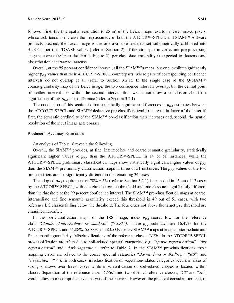
Remote Sens. 2013, 5 5241
follows. First, the fine spatial resolution (0.25 m) of the Leica image results in fewer mixed pixels,
whose lack tends to increase the map accuracy of both the ATCOR™-SPECL and SIAM™ software
products. Second, the Leica image is the sole available test data set radiometrically calibrated into
SURF rather than TOARF values (refer to Section 2). If the atmospheric correction pre-processing
stage is correct (refer to the Part 1, Figure 2), per-class data variability is expected to decrease and
classification accuracy to increase.
Overall, at the 95 percent confidence interval, all the SIAM™’s maps, but one, exhibit significantly
higher values than their ATCOR™-SPECL counterparts, where pairs of corresponding confidence
intervals do not overlap at all (refer to Section 3.2.1). In the single case of the Q-SIAM™
coarse-granularity map of the Leica image, the two confidence intervals overlap, but the central point
of neither interval lies within the second interval, thus we cannot draw a conclusion about the
significance of this pair difference (refer to Section 3.2.1).
The conclusion of this section is that statistically significant differences in estimates between
the ATCOR™-SPECL and SIAM™ deductive pre-classifiers tend to increase in favor of the latter if,
first, the semantic cardinality of the SIAM™ pre-classification map increases and, second, the spatial
resolution of the input image gets coarser.
Producer’s Accuracy Estimation
An analysis of Table 16 reveals the following.
Overall, the SIAM™ provides, at fine, intermediate and coarse semantic granularity, statistically
significant higher values of than the ATCOR™-SPECL in 14 of 51 instances, while the
ATCOR™-SPECL preliminary classification maps show statistically significant higher values of
than the SIAM™ preliminary classification maps in three of 51 instances. The values of the two
pre-classifiers are not significantly different in the remaining 34 cases.
The adopted requirement of 70% ± 5% (refer to Section 3.2.1) is exceeded in 15 out of 17 cases
by the ATCOR™-SPECL, with one class below the threshold and one class not significantly different
than the threshold at the 99 percent confidence interval. The SIAM™ pre-classification maps at coarse,
intermediate and fine semantic granularity exceed this threshold in 49 out of 51 cases, with two
reference LC classes falling below the threshold. The four cases not above the target threshold are
examined hereafter.
In the pre-classification maps of the IRS image, index scores low for the reference
class “Clouds, cloud-shadows or shadows” (“Cl/Sh”). These estimates are 16.47% for the
ATCOR™-SPECL and 55.88%, 55.88% and 83.53% for the SIAM™ maps at coarse, intermediate and
fine semantic granularity. Misclassifications of the reference class “Cl/Sh” in the ATCOR™-SPECL
pre-classification are often due to soil-related spectral categories, e.g., “sparse vegetation/soil”, “dry
vegetation/soil” and “dark vegetation”, refer to Table 2. In the SIAM™ pre-classifications these
mapping errors are related to the coarse spectral categories “Barren land or Built-up” (“BB”) and
“Vegetation” (“V”). In both cases, misclassification of vegetation-related categories occurs in areas of
strong shadows over forest cover while misclassification of soil-related classes is located within
clouds. Separation of the reference class “Cl/Sh” into two distinct reference classes, “Cl” and “Sh”,
would allow more comprehensive analysis of these errors. However, the practical consideration that, in
Remote Sens. 2013, 5 5242
the IRS test image, the occurrence of this reference class is below the minimum per-class sample size
of 340 pixels required by the modified SIRS strategy implemented in this work makes a split of
parent-class “Cl/Sh” into child-classes Cl” and “Sh” impractical (refer to Section 3.2.1). Alternatively,
a “fuzzy” reference labeling scheme which applies more than one label to a reference sample could be
implemented. Unfortunately, whereas the construction of an OAMTRX/CMTRX is straightforward
and non-controversial when the semantic labels of sampling units are crisp (hard), the method to
construct an OAMTRX/CMTRX is not obvious at all when semantic labels are soft (fuzzy) [32,34].
Table 16. Producer’s Accuracy = = Equation (11) ±δ = Equation (5) for the
ATCOR™-SPECL and SIAM™ pre-classifications of the three test images with α = RC/100,
1 − α/RC = 0.99, χ2(1, 1-α/RC) = 6.63 in Equation (5).
IRS-P6 LISS-3, 23.5 m-Resolution,
4-Band (G, R, NIR, MIR), Reference LC Classes (Refer to Table 5)
ATCOR™-
SPECL
(19 sp. cat.) ,
PPA = Eq. (11)
+/− δ =
Eq. (5)
S-SIAM™(Coarse =
15 sp. cat.) ,
PPA = Eq. (11)
+/− δ =
Eq. (5)
S-SIAM™(Interm.
=
40 sp. cat.) ,
PPA = Eq. (11)
+/− δ =
Eq. (5)
S-SIAM™ (Fine =
68 sp. cat.) ,
PPA = Eq. (11)
+/− δ =
Eq. (5)
Number of
Randomly Selected
Reference
Samples (Spatial
Type: Pixel)
Cl/Sh 16.47% 5.18% 55.88% 6.93% 55.88% 6.93% 83.53% 5.18% 340
BBS 99.41% 1.07% 94.12% 3.29% 94.12% 3.29% 98.24% 1.84% 340
Range/MP 97.94% 1.98% 99.71% 0.76% 99.71% 0.76% 99.71% 0.76% 340
VL-M NIR 98.53% 1.68% 98.53% 1.68% 99.71% 0.76% 100.00% 0.00% 340
H-VH NIR 100.00% 0.00% 99.71% 0.76% 100.00% 0.00% 100.00% 0.00% 340
Water 93.24% 3.51% 95.00% 3.04% 99.41% 1.07% 99.41% 1.07% 340
SPOT-4 HRVIR, 20 m-Resolution,
4-Band (G, R, NIR, MIR), Reference LC Classes (Refer to Table 6)
ATCOR™-
SPECL
(19 sp. cat.) ,
PPA = Eq. (11)
+/− δ =
Eq. (5)
S-SIAM™(Coarse =
15 sp. cat.) ,
PPA = Eq. (11)
+/− δ =
Eq. (5)
S-SIAM™(Interm.
=
40 sp. cat.) ,
PPA = Eq. (11)
+/− δ =
Eq. (5)
S-SIAM™ (Fine =
68 sp. cat.) ,
PPA = Eq. (11)
+/− δ =
Eq. (5)
Number of
Randomly Selected
Reference
Samples (Spatial
Type: Pixel)
BBS 98.82% 1.51% 94.41% 3.21% 94.41% 3.21% 97.65% 2.12% 340
Range/MP 97.65% 2.12% 100.00% 0.00% 100.00% 0.00% 100.00% 0.00% 340
VL-M NIR 99.71% 0.76% 100.00% 0.00% 100.00% 0.00% 100.00% 0.00% 340
H-VH NIR 100.00% 0.00% 100.00% 0.00% 100.00% 0.00% 100.00% 0.00% 340
Water 63.82% 6.71% 82.94% 5.25% 99.12% 1.31% 99.12% 1.31% 340
Leica ADS-80,
0.25 m-Resolution,
4-Band (B, G, R, NIR), Reference LC Classes (Refer to Table 7)
ATCOR™-
SPECL
(19 sp. cat.) ,
PPA = Eq. (11)
+/− δ =
Eq. (5)
Q-SIAM™(Coarse =
12 sp. cat.) ,
PPA =
Eq. (11)
+/− δ =
Eq. (5)
Q-SIAM™(Interm.
=
28 sp. cat.) ,
PPA =
Eq. (11)
+/− δ =
Eq. (5)
Q-SIAM™ (Fine =
52 sp. cat.) ,
PPA =
Eq. (11)
+/− δ =
Eq. (5)
Number of
Randomly Selected
Reference
Samples (Spatial
Type: Pixel)
LtBBrS 99.71% 0.76% 97.94% 1.98% 97.94% 1.98% 97.94% 1.98% 340
DkBDkS 79.71% 5.62% 97.65% 2.12% 97.35% 2.24% 97.35% 2.24% 340
NDVI1 100.00% 0.00% 100.00% 0.00% 100.00% 0.00% 100.00% 0.00% 340
NDVI2 98.82% 1.51% 100.00% 0.00% 100.00% 0.00% 100.00% 0.00% 340
TrCr 100.00% 0.00% 100.00% 0.00% 100.00% 0.00% 100.00% 0.00% 340
SH 98.53% 1.68% 99.41% 1.07% 99.41% 1.07% 89.71% 4.24% 340
Outlier -- -- -- -- 5
Remote Sens. 2013, 5 5243
To summarize, the SIAM™ appears capable of outperforming the ATCOR™-SPECL in the color
mapping of clouds and cloud-shadows. However, both first-stage deductive pre-classifiers are not
expected to be successful as cloud detectors based on per-pixel (color) properties exclusively, while
spatial information is ignored. This means that, to detect clouds effectively, a second-stage
context-sensitive one-class cloud detection classifier, driven by the SIAM™’s first-stage knowledge,
should be developed in compliance with the novel hybrid RS-IUS architecture proposed in [10–19]
(refer to the Part 1, Section 4.1).
With regard to the multi-granule pre-classification of the SPOT test image, Table 16 shows that
indicators are lower than expected for the reference LC class “Water” in the ATCOR™-SPECL map
(62.82% ± 6.71%) and the SIAM™ map at coarse granularity (82.94% ± 5.25%). In this reference LC
class, misclassifications occur with spectral category “Asphalt/dark sand” for the ATCOR™-SPECL
and spectral category “Thin cloud over shrub-rangeland or herbaceous rangeland or bare soil and
built-up” (“TNCL_SHRBR_HRBCR_BB”) for the SIAM™ maps, respectively.
Finally, in the pre-classification maps of the Leica image, all indicators far exceed the
70% ± 5% per-class accuracy target (refer to Section 3.2.1). Slight decreases in performance are
observed in the ATCOR™-SPECL pre-classification map overlapping with the reference LC class
“Dark Built-up or Dark Soil” (“DkBDkS”) (79.71% ± 5.62%, with misclassification errors attributed to
the spectral category “not classified”. Similarly, the SIAM™ pre-classification map at fine semantic
granularity demonstrates a value below average for the LC class “Shadow” (“SH”). Many
so-called errors in this LC class are due to spectral category “Average shrub-rangeland with very low
near-infrared response” (“ASHRBRVLNIR”), which actually features a spectral overlap with
vegetation in shadow, since the SIAM™ is capable of “looking-through” both haze/thin clouds and
shadows (refer to the Part 1, Section 4.2.1 [20]). To say that this spectral category should be no longer
considered as a source of errors for the detection of the LC class “SH”. This case is proposed as an
example of reference-test class relation, subjectively interpreted as “incorrect” by a knowledge
engineer, which would deserve to be reconsidered to become community-agreed upon. If the
reference-test class pair (“SH”, “ASHRBRVLNIR”) is considered as a “correct” entry, then TQI values,
like and , are expected to increase at the cost of a decrease of the CVPSI value. This
combination of effects should be carefully assessed by the domain expert, because mutually
independent TQIs, SQIs and the CVPSI should be maximized simultaneously (also refer to
Section 3.1.2).
User’s Accuracy Estimation
Complete measures are accessible via anonymous ftp [52]. While is a useful TQI for many
purposes (refer to the introduction to Section 3.4.1), the adopted probability sampling design specifies
the cardinality of reference rather than test classes (refer to Section 3.2.1). The consequence is that
while it is ensured that each reference category obtains a minimum of 340 samples, for practical
reasons no such requirement is imposed for test categories. For example, with a possible 68 output
spectral categories in an S-SIAM™ map at fine semantic granularity (refer to Table 3), user’s accuracy
assessment could require up to 340 × 68 = 23,120 samples overall, according to the Lunetta and
Elvidge sample size estimation criterion (refer to Section 3.2.1). As a result, in the test maps at hand
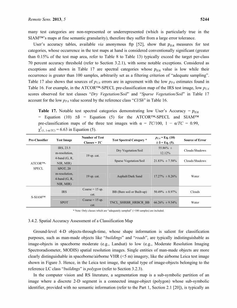
Remote Sens. 2013, 5 5244
many test categories are non-represented or underrepresented (which is particularly true in the
SIAM™’s maps at fine semantic granularity), therefore they suffer from a large error tolerance.
User’s accuracy tables, available via anonymous ftp [52], show that measures for test
categories, whose occurrence in the test maps at hand is considered conventionally significant (greater
than 0.15% of the test map area, refer to Table 8 to Table 13) typically exceed the target per-class
70 percent accuracy threshold (refer to Section 3.2.1), with some notable exceptions. Considered as
exceptions and shown in Table 17 are spectral categories whose value is low while their
occurrence is greater than 100 samples, arbitrarily set as a filtering criterion of “adequate sampling”.
Table 17 also shows that sources of pUA errors are in agreement with the low pPA estimates found in
Table 16. For example, in the ATCOR™-SPECL pre-classification map of the IRS test image, low pUA
scores observed for test classes “Dry Vegetation/Soil” and “Sparse Vegetation/Soil” in Table 17
account for the low pPA value scored by the reference class “Cl/Sh” in Table 16.
Table 17. Notable test spectral categories demonstrating low User’s Accuracy =
= Equation (10) ±δ = Equation (5) for the ATCOR™-SPECL and SIAM™
pre-classification maps of the three test images with α = TC/100, 1 − α/TC = 0.99,
χ2(1, 1-α/TC) = 6.63 in Equation (5).
Pre-Classifier Test Image Number of Test
Classes = TC Test Spectral Category *
pUA = Eq. (10)
± δ = Eq. (5). Source of Error
ATCOR™-
SPECL
IRS, 23.5
m-resolution,
4-band (G, R,
NIR, MIR)
19 sp. cat.
Dry Vegetation/Soil 55.86% ±
12.12% Clouds/Shadows
Sparse Vegetation/Soil 21.83% ± 7.58% Clouds/Shadows
SPOT, 20
m-resolution,
4-band (G, R,
NIR, MIR)
19 sp. cat. Asphalt/Dark Sand 17.27% ± 8.26% Water
S-SIAM™
IRS Coarse = 15 sp.
cat. BB (Bare soil or Built-up) 50.49% ± 8.97% Clouds
SPOT Coarse = 15 sp.
cat. TNCL_SHRBR_HRBCR_BB 66.26% ± 9.54% Water
* Note: Only classes which are “adequately sampled” (>100 samples) are included.
3.4.2. Spatial Accuracy Assessment of a Classification Map
Ground-level 4-D objects-through-time, whose shape information is salient for classification
purposes, such as man-made objects like “buildings” and “roads”, are typically indistinguishable as
image-objects in spaceborne moderate (e.g., Landsat) to low (e.g., Moderate Resolution Imaging
Spectroradiometer, MODIS) spatial resolution images. Single entities of man-made objects are more
clearly distinguishable in spaceborne/airborne VHR (<5 m) imagery, like the airborne Leica test image
shown in Figure 3. Hence, in the Leica test image, the spatial type of image-objects belonging to the
reference LC class “buildings” is polygon (refer to Section 3.2.3).
In the computer vision and RS literature, a segmentation map is a sub-symbolic partition of an
image where a discrete 2-D segment is a connected image-object (polygon) whose sub-symbolic
identifier, provided with no semantic information (refer to the Part 1, Section 2.1 [20]), is typically an
Remote Sens. 2013, 5 5245
integer number, e.g., segment 1, segment 2, etc. Notably, a unique (sub-symbolic) segmentation map
can be generated from a (symbolic) thematic map (binary or multi-level image) [31], but the contrary
does not hold because different thematic maps can generate the same segmentation map, i.e., no
thematic map can be unequivocally inferred from a segmentation map (refer to the Part 1,
Section 4.4).
In compliance with the original protocol proposed in [32], a set of sub-symbolic polygon-based
SQIs is estimated in the 2-D pre-classification map domain independently of a set of traditional
symbolic pixel-based TQIs extracted from an OAMTRX instance (refer to Section 3.4.1). Proposed
SQIs are independent one another, to cope with the non-injective property of any QI (refer to the
Part 1, Section 2.5 [20]), and are provided with a degree of uncertainty in measurement in compliance
with the principles of statistics and the QA4EO guidelines [2].
SQI Formulations
In typical geographic object-based image analysis (GEOBIA) applications [59–66] (refer to the
Part 1, Section 2.2 [20]), like building detection in VHR images, possible SQI formulations are
proposed by McGlone and Shufelt in [67] and applied by Hermosilla et al. [68]. Inversely related to
spatial error indices originally presented by Persello and Bruzzone in the RS literature [55], four
general-purpose global SQIs are proposed in [32]. A global (image-wide) SQI is computed as the mean
of the sum over all the values of a local SQI estimator. A local SQI estimator investigates a specific
spatial relationship, e.g., oversegmentation, undersegmentation or edge mis-location, between the i-th reference image-object belonging to a reference LC class , RO , , and its corresponding target
(mapped) image-object, identified as , , located in the test segmentation map as the sub-symbolic
segment with the most pixels in common with the reference object, such that [55]: , = ∀ ∈ , ∩ , = 1,… , , = 1,… , ( ) (12)
where symbol |∙| represents the set cardinality, namely, the size of the segment-pair overlapping area,
and RT(c) is the total number of reference objects in reference class c, with c = 1, ..., RC. Therefore, a
reference class-specific global SQI is computed as:
= 1( ) , , , ,( ) , , , , , ∈ (0,1], ∈ (0,1],= 1,… ,
(13)
It is worth mentioning that this global SQI formulation accounts for the polygon-specific inclusion
probability, which increases with the polygon size and whose inverse value determines the weight
attached to each sampling unit in probability sampling [32].
The four local SQI estimators proposed in [32] are summarized hereafter. Inversely related to the
oversegmentation error presented in [55], the local Oversegmentation SQI (OSQI) estimator quantifies the degree of overlap between , and , with respect to , [32].
, ( , , , ) = , ∩ ,, ∈ (0,1], = 1,… , (14)
Remote Sens. 2013, 5 5246
Complementary to the local OSQI function, the local Undersegmentation SQI (USQI) estimator is
inversely related to the undersegmentation error presented in [55]. In practice, observed OSQI and
USQI values tend to be inversely related, though this observed relationship is not axiomatic (which is
evidence that the OSQI and USQI are in fact not correlated). The local USQI quantifies the degree of overlap between , and , with respect to , .
, ( , , , ) = , ∩ ,, ∈ (0,1], = 1, … , (15)
Image-contour detection is the dual problem of image-object segmentation [10–19]. Inspired to the
edge location error index presented in [55], two Fuzzy Edge Overlap SQIs (FEOQIs) measure the
precision (inverse of distance) of the contour of the target object relative to the contour of the reference
object and vice versa. For the purpose of edge extraction, a buffer half-width distance parameter,
represented as (∙), must be user-defined. The included buffer distance is necessary to create an areal
object around an edge (since edges are lines, hence have no thickness), but is also useful for reducing
the impact of accidental spatial errors inevitably introduced in the localization of reference contours
through human photointerpretation. It is worth noting that while the buffer half-width distance is a free
parameter to be user-defined, the value of should be as small as possible to avoid inflating FEOQI
values. For example, 2 pixels seems a reasonable buffer half-width in the Leica test image whose
spatial resolution is 0.25 m, therefore is set equal to 0.50 m. The first local FEOQI estimator, called
FEOQI_Reference (FEOQI_R) ∈ (0, 1), which quantifies the similarity between reference and test
object edges with respect to the reference object, is computed as follows [32]. _ , ( , , , ) = ( , ) ∩ ( , )( , ) ∈ (0,1], = 1, … , . (46)
The second local FEOQI estimator, called FEOQI_Test (FEOQI_T) ∈ (0, 1], which quantifies the
similarity between reference and test object edges with respect to the test object is the dual function of
the FEOQI_R estimator. It is computed as follows [32]. _ , ( , , , ) = ( , ) ∩ ( , )( , ) ∈ (0,1], = 1,… , . (17)
The goal of an image segmentation algorithm would be to maximize the aforementioned SQIs up to
value 1 (whereas error indices, like those in [55], should be minimized to 0), where 1 represents
perfect agreement (with respect to the divisor) between reference and target objects. In the worst case
scenario, where only one pixel is in common between every reference and mapped object pair, SQIs
approach zero. The four proposed local SQI estimators are shown in Figure 5. For example, in Figure 5a, there is perfect agreement between the areas of the , and , with respect to , , but
not with respect to , . Hence, in Figure 5a, , ( , , , ) is expected to be “low” while , ( , , , ) is expected to tend to 1.
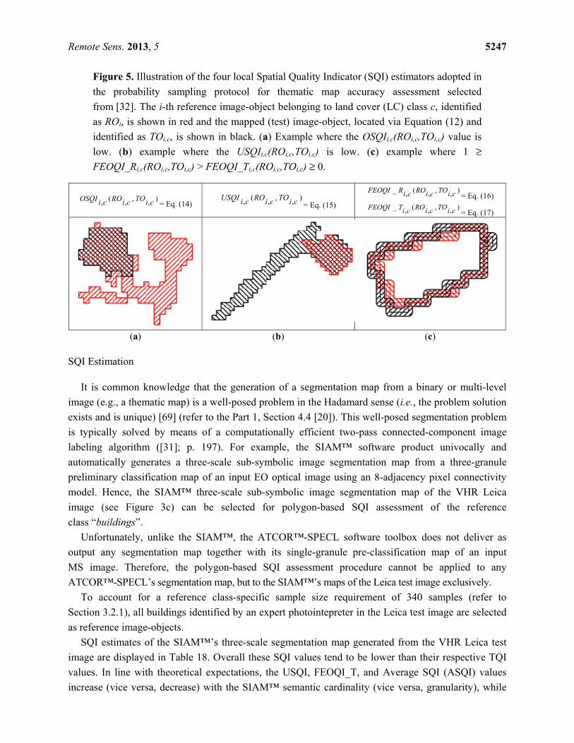
Remote Sens. 2013, 5 5247
Figure 5. Illustration of the four local Spatial Quality Indicator (SQI) estimators adopted in
the probability sampling protocol for thematic map accuracy assessment selected
from [32]. The i-th reference image-object belonging to land cover (LC) class c, identified
as ROi, is shown in red and the mapped (test) image-object, located via Equation (12) and
identified as TOi,c, is shown in black. (a) Example where the OSQIi,c(ROi,c,TOi,c) value is
low. (b) example where the USQIi,c(ROi,c,TOi,c) is low. (c) example where 1 ≥
FEOQI_Ri,c(ROi,c,TOi,c) > FEOQI_Ti,c(ROi,c,TOi,c) ≥ 0.
),,,(, ciTOciROciOSQI= Eq. (14)
),,,(, ciTOciROciUSQI= Eq. (15)
),,,(,_ ciTOciROciRFEOQI= Eq. (16)
),,,(,_ ciTOciROciTFEOQI= Eq. (17)
(a) (b) (c)
SQI Estimation
It is common knowledge that the generation of a segmentation map from a binary or multi-level
image (e.g., a thematic map) is a well-posed problem in the Hadamard sense (i.e., the problem solution
exists and is unique) [69] (refer to the Part 1, Section 4.4 [20]). This well-posed segmentation problem
is typically solved by means of a computationally efficient two-pass connected-component image
labeling algorithm ([31]; p. 197). For example, the SIAM™ software product univocally and
automatically generates a three-scale sub-symbolic image segmentation map from a three-granule
preliminary classification map of an input EO optical image using an 8-adjacency pixel connectivity
model. Hence, the SIAM™ three-scale sub-symbolic image segmentation map of the VHR Leica
image (see Figure 3c) can be selected for polygon-based SQI assessment of the reference
class “buildings”.
Unfortunately, unlike the SIAM™, the ATCOR™-SPECL software toolbox does not deliver as
output any segmentation map together with its single-granule pre-classification map of an input
MS image. Therefore, the polygon-based SQI assessment procedure cannot be applied to any
ATCOR™-SPECL’s segmentation map, but to the SIAM™’s maps of the Leica test image exclusively.
To account for a reference class-specific sample size requirement of 340 samples (refer to
Section 3.2.1), all buildings identified by an expert photointepreter in the Leica test image are selected
as reference image-objects.
SQI estimates of the SIAM™’s three-scale segmentation map generated from the VHR Leica test
image are displayed in Table 18. Overall these SQI values tend to be lower than their respective TQI
values. In line with theoretical expectations, the USQI, FEOQI_T, and Average SQI (ASQI) values
increase (vice versa, decrease) with the SIAM™ semantic cardinality (vice versa, granularity), while
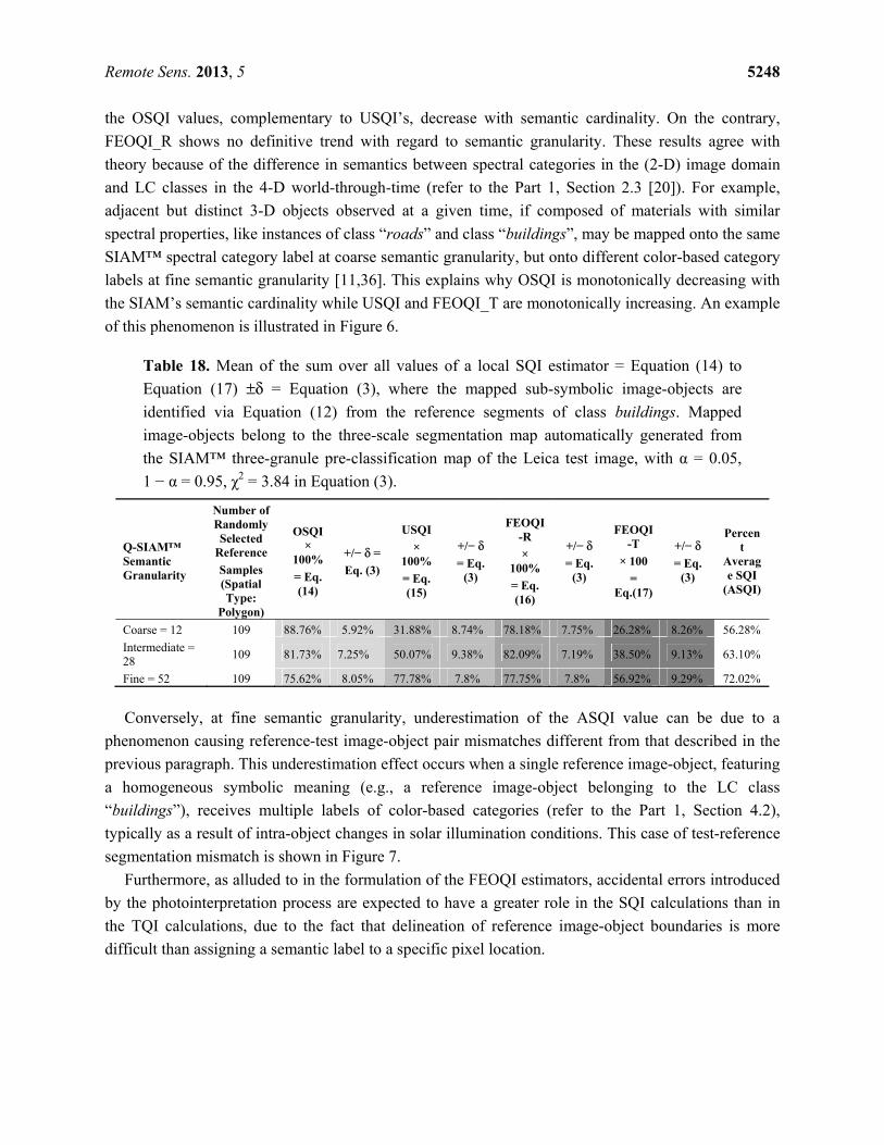
Remote Sens. 2013, 5 5248
the OSQI values, complementary to USQI’s, decrease with semantic cardinality. On the contrary,
FEOQI_R shows no definitive trend with regard to semantic granularity. These results agree with
theory because of the difference in semantics between spectral categories in the (2-D) image domain
and LC classes in the 4-D world-through-time (refer to the Part 1, Section 2.3 [20]). For example,
adjacent but distinct 3-D objects observed at a given time, if composed of materials with similar
spectral properties, like instances of class “roads” and class “buildings”, may be mapped onto the same
SIAM™ spectral category label at coarse semantic granularity, but onto different color-based category
labels at fine semantic granularity [11,36]. This explains why OSQI is monotonically decreasing with
the SIAM’s semantic cardinality while USQI and FEOQI_T are monotonically increasing. An example
of this phenomenon is illustrated in Figure 6.
Table 18. Mean of the sum over all values of a local SQI estimator = Equation (14) to
Equation (17) ±δ = Equation (3), where the mapped sub-symbolic image-objects are
identified via Equation (12) from the reference segments of class buildings. Mapped
image-objects belong to the three-scale segmentation map automatically generated from
the SIAM™ three-granule pre-classification map of the Leica test image, with α = 0.05,
1 − α = 0.95, χ2 = 3.84 in Equation (3).
Q-SIAM™ Semantic Granularity
Number of Randomly Selected
Reference
Samples (Spatial Type:
Polygon)
OSQI ×
100%
= Eq. (14)
+/− δ =
Eq. (3)
USQI
× 100%
= Eq. (15)
+/− δ
= Eq. (3)
FEOQI-R
× 100%
= Eq. (16)
+/− δ
= Eq. (3)
FEOQI-T
× 100
= Eq.(17)
+/− δ
= Eq. (3)
Percent
Average SQI
(ASQI)
Coarse = 12 109 88.76% 5.92% 31.88% 8.74% 78.18% 7.75% 26.28% 8.26% 56.28%
Intermediate = 28
109 81.73% 7.25% 50.07% 9.38% 82.09% 7.19% 38.50% 9.13% 63.10%
Fine = 52 109 75.62% 8.05% 77.78% 7.8% 77.75% 7.8% 56.92% 9.29% 72.02%
Conversely, at fine semantic granularity, underestimation of the ASQI value can be due to a
phenomenon causing reference-test image-object pair mismatches different from that described in the
previous paragraph. This underestimation effect occurs when a single reference image-object, featuring
a homogeneous symbolic meaning (e.g., a reference image-object belonging to the LC class
“buildings”), receives multiple labels of color-based categories (refer to the Part 1, Section 4.2),
typically as a result of intra-object changes in solar illumination conditions. This case of test-reference
segmentation mismatch is shown in Figure 7.
Furthermore, as alluded to in the formulation of the FEOQI estimators, accidental errors introduced
by the photointerpretation process are expected to have a greater role in the SQI calculations than in
the TQI calculations, due to the fact that delineation of reference image-object boundaries is more
difficult than assigning a semantic label to a specific pixel location.
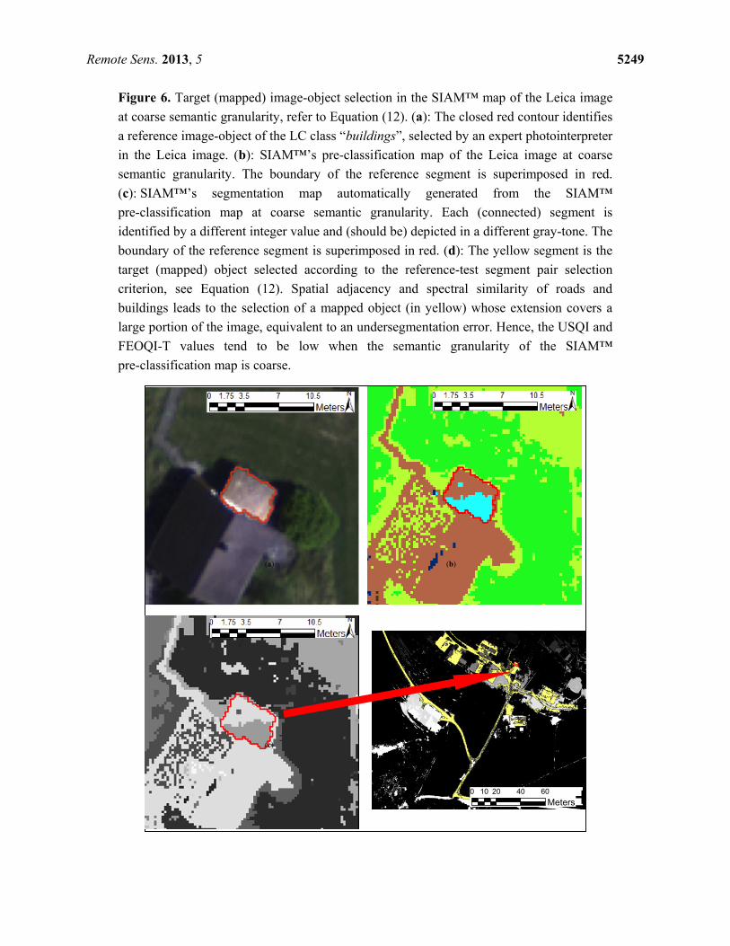
Remote Sens. 2013, 5 5249
Figure 6. Target (mapped) image-object selection in the SIAM™ map of the Leica image
at coarse semantic granularity, refer to Equation (12). (a): The closed red contour identifies
a reference image-object of the LC class “buildings”, selected by an expert photointerpreter
in the Leica image. (b): SIAM™’s pre-classification map of the Leica image at coarse
semantic granularity. The boundary of the reference segment is superimposed in red.
(c): SIAM™’s segmentation map automatically generated from the SIAM™
pre-classification map at coarse semantic granularity. Each (connected) segment is
identified by a different integer value and (should be) depicted in a different gray-tone. The
boundary of the reference segment is superimposed in red. (d): The yellow segment is the
target (mapped) object selected according to the reference-test segment pair selection
criterion, see Equation (12). Spatial adjacency and spectral similarity of roads and
buildings leads to the selection of a mapped object (in yellow) whose extension covers a
large portion of the image, equivalent to an undersegmentation error. Hence, the USQI and
FEOQI-T values tend to be low when the semantic granularity of the SIAM™
pre-classification map is coarse.
±0 20 40 6010Meters
(a) (b)
(c)
(d)
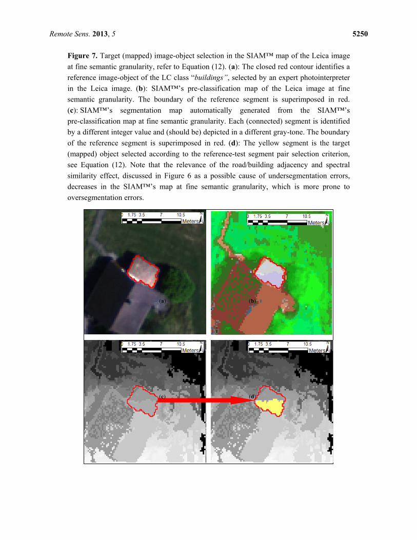
Remote Sens. 2013, 5 5250
Figure 7. Target (mapped) image-object selection in the SIAM™ map of the Leica image
at fine semantic granularity, refer to Equation (12). (a): The closed red contour identifies a
reference image-object of the LC class “buildings”, selected by an expert photointerpreter
in the Leica image. (b): SIAM™’s pre-classification map of the Leica image at fine
semantic granularity. The boundary of the reference segment is superimposed in red.
(c): SIAM™’s segmentation map automatically generated from the SIAM™’s
pre-classification map at fine semantic granularity. Each (connected) segment is identified
by a different integer value and (should be) depicted in a different gray-tone. The boundary
of the reference segment is superimposed in red. (d): The yellow segment is the target
(mapped) object selected according to the reference-test segment pair selection criterion,
see Equation (12). Note that the relevance of the road/building adjacency and spectral
similarity effect, discussed in Figure 6 as a possible cause of undersegmentation errors,
decreases in the SIAM™’s map at fine semantic granularity, which is more prone to
oversegmentation errors.
(a) (b)
(c) (d)
Remote Sens. 2013, 5 5251
3.4.3. Remarks
Based on a realistic many-to-many association model (represented by “correct” entries distributed
across an OAMTRX instance, refer to Section 3.1) between a pair of test and reference semantic
vocabularies which, in general, may not coincide (refer to the Part 1, Section 4.2 [20]), symbolic
pixel-based TQIs, collected in this section, are: (i) inversely related to so-called “quantification
errors” [53,54], and (ii) insensitive to the geospatial distribution of errors, related to the so-called
“location error” [53,54], refer to the introduction to Section 3.4.
On the other hand, based on a one-to-one association model between one reference polygon and one
mapped sub-symbolic polygon, see Equation (12), sub-symbolic polygon-specific SQIs, collected in
this section, are: (i) inversely related to “location errors”, estimated according to Equations (12–17),
and (ii) insensitive to so-called “quantification errors” [53,54]. For example, SQIs are independent of
the semantic label of the mapped polygon detected via Equation (12), i.e., they are insensitive to
whether or not the pair of semantic labels of the reference and mapped objects identifies a “correct”
entry in the OAMTRX instance at hand.
Moreover, Equation (12), adopted to detect a sub-symbolic mapped polygon of a reference polygon,
is unable to capture any possible “correct” one-to-many association between one polygon belonging to
a specific reference class (e.g., an LC class) with one or more polygons belonging to a set of “correct”
test classes (e.g., spectral categories). This means that, based on theoretical considerations exclusively,
in the second type of inter-map comparisons described in the introduction to Section 3.1, where
reference and test thematic vocabularies do not coincide and where one-to-many reference-to-test class
relations (e.g., one LC class maps into several spectral categories) can be considered “correct”, in
agreement with the CVPSI2 formulation proposed in the Appendix, SQIs computed according to
Equations (12–17) are expected to be negatively biased (i.e., underestimated), whereas the same SQI
formulas have no bias when applied to the first type of inter-map comparisons, described in the
introduction to Section 3.1, where one-to-one test-reference class relations can be found exclusively.
To conclude this section, in a thematic map accuracy assessment task, where many-to-many
associations typically hold between reference LC classes and test classes, like in Tables 8–13, it is
reasonable to expect that estimated TQI values are higher than SQI estimates, because the latter are,
first, better suited to cope with one-to-one inter-vocabulary associations and, second, negatively
affected by undesired effects (like those shown in Figures 6 and 7). This may explain why, in the
proposed experiments, the ASQI values reported in Table 18 are significantly lower than TQI values
shown in Tables 15 and 16.
4. QIOs Assessment
In agreement with the Part 1, Section 2.5 [20], a set of QIOs is selected and instantiated for the
comparison of the ATCOR™-SPECL and SIAM™ software products in operating mode, to comply
with the QA4EO guidelines (refer to the Part 1, Section 3 [20]).
Since the ATCOR™-SPECL and SIAM™ static decision-tree pre-classifiers share the abstraction
levels of computational theory and, to some degree, knowledge/information representation, but differ
at the abstraction levels of algorithms and implementation (refer to the Part 1, Section 4 [20]), their
Remote Sens. 2013, 5 5252
corresponding QIO values are expected to be different, but “similar”, which means they are expected
to share the same order of magnitude.
Estimated QIOs of the ATCOR™-SPECL and SIAM™ software products are compared as follows.
(i) Degree of automation. It is estimated as the inverse of the number of system
free-parameters to be user-defined, which is null, hence degree of automation is
maximum, i.e., it cannot be surpassed by alternative approaches. Both preliminary
classifiers are termed “fully automatic” [21], i.e., they require neither input parameters
to be user-defined nor training data to run (refer to the Part 1, Section 4.1 [20]).
(ii) Effectiveness, intended as accuracy of the pre-classification map. Map accuracy
measures are split into independent QIs, namely, TQIs, SQIs and the CVSPI, see
Section 3. The TQI values of the SIAM™ tend to be significantly higher (in statistical
terms) than the ATCOR™-SPECL’s. Also the CVPSI values of the SIAM™ at the
intermediate and fine semantic granularities are higher than those of the
ATCOR™-SPECL single-granule maps. Estimated for the SIAM™ exclusively, SQIs
tend to be lower than their corresponding TQIs (refer to Section 3.4.2).
(iii) Efficiency is estimated as the inverse of computation time, because memory
occupation is negligible, both algorithms being pixel-based. The two deductive
pre-classifiers are context-insensitive (pixel-based), non-iterative (one-pass) and
non-adaptive to input data (prior knowledge-based), hence they are computationally
efficient. For example, in a laptop computer provided with a Windows operating
system, SIAM™ requires three minutes to generate as output three pre-classification
maps from a 7-band Landsat full scene, approximately 7,000 × 7,000 pixels in size. In
practice, both pre-classifiers can be considered near real-time.
(iv) Robustness to changes in input parameters cannot be surpassed by alternative
approaches, because no system free-parameter exists.
(v) Robustness to changes in input data acquired across time, space and sensors is
investigated in Section 3, in addition to the existing literature [6–19]. It can be
considered (qualitatively) “high”. This is due to a combination of effects. First, the
required radiometric calibration constraint guarantees harmonization of MS data
acquired across time, space and sensors (refer to the Part 1, Section 4.2.1 [20]).
Second, the two pre-classifiers are pixel-based, i.e., both systems work at the spatial
resolution of the imaging sensor whatever it is, i.e., they are spatial
resolution-independent. Third, the two rule-based mapping system implementations
pursue redundancy of the rule set. Actually, redundancy of the SIAM™ rule set
appears far superior to that of the ATCOR™-SPECL rule set at the expense of a higher
level of software complexity of the former. In practice, both systems are eligible for
use with any existing or future planned spaceborne/airborne optical mission whose
spectral resolution overlaps with Landsat’s, irrespective of spatial resolution (e.g.,
refer to the Part 1, Table 3 and the Part 1, Table 4 [20]). For example, starting from a
Landsat spectral resolution of seven bands, ranging from visible to thermal
electromagnetic wavelengths (refer to the Part 1, Tables 3 and 4 [20]), the SIAM™
Remote Sens. 2013, 5 5253
decision tree can work with as low as two input bands, namely, one visible and one NIR
channel [12–14].
(vi) Scalability, to cope with changes in sensor specifications, is investigated in Section 3,
in addition to the existing literature [6–19]. It can be considered “high”, for the same
reasons of point (v).
(vii) Timeliness, from data acquisition to data-derived high-level product generation, is
equivalent to computation time, because user interactions are zero. Since their
computation time is low then their timeliness is extremely favorable (“low”).
(viii) Costs. The combination of high computation efficiency with no user interactions
implies that costs in computer power and manpower are “low”.
To summarize, according to collected QIO values, including CVPSI, TQI and SQI values (refer to
Section 3), the ATCOR™-SPECL and SIAM™ deductive pre-classifiers accomplish automatic and
near real-time detection of spectral categories in an input single-date MS imagery, where automation
does not come at the expense of accuracy, robustness to changes in the input data set or scalability, but
at the expense of the informative content of the output spectral-based semi-concepts whose semantic
meaning is “low”, namely, is equal or inferior to that of target 4-D LC classes-through-time (refer to
the Part 1, Section 2.3 [20]). In the proposed set of experiments, the CVPSI and TQI values of the
SIAM™ tend to outperform those of the ATCOR™-SPECL.
5. Conclusions
The primary objective of this paper is to provide, in accordance with the Quality Assurance
Framework for Earth Observation (QA4EO) guidelines [2], a quality assessment of two alternative
operational (turnkey, ready-to-go) software products: the Spectral Classification of surface reflectance
signatures (SPECL) and the Satellite Image Automatic Mapper™ (SIAM™). The former is
implemented as a non-validated secondary product within the Atmospheric/Topographic Correction
(ATCOR™)-2/3/4 commercial software toolbox [6–8,9]. The latter has been presented in recent years
in the remote sensing (RS) literature [10–19], where enough information is provided for the SIAM™
implementation to be reproduced [11,17].
To the best of these authors’ knowledge, the ATCOR™-SPECL and SIAM™ software products are
the only two pre-attentive vision expert systems (deductive inference systems for pre-attentional
vision) in operating mode made available to date to the remote sensing (RS) community for “fully
automatic” near real-time preliminary classification (pre-classification) of radiometrically calibrated
spaceborne/airborne multi-resolution MS images. “Fully automatic" means that the pre-attentional data
mapping system requires neither user-defined parameters nor training data sample to run [21].
For the sake of simplicity, this paper is split into two: Part 1—Theory [20] and the present
Part 2—Experimental results.
The Part 1 provides the present Part 2 with an interdisciplinary terminology and a theoretical
background. To comply with the principle of statistics and the QA4EO guidelines discussed in the
Part 1 [20], the present Part 2 applies a novel probability sampling protocol for thematic map quality
assessment, selected from the recent literature [32], to the ATCOR™-SPECL and SIAM™
pre-classification maps. Three sets of independent metrological/statistically-based quality indicators
Remote Sens. 2013, 5 5254
(QIs) are estimated to investigate the mapping effectiveness (accuracy) of the ATCOR™-SPECL and
SIAM™ deductive pre-classifiers.
A Categorical Variable Pair Similarity Index (CVPSI) ∈ [0, 1]. The CVPSI is a normalized
estimate of the degree of semantic harmonization (reconciliation) between the test
and reference class taxonomies which, in general, may not coincide. Vice versa,
(1 − CVPSI) ∈ [0, 1] is a normalized estimate of the residual of the semantic gap from
sub-symbolic data to symbolic reference classes filled up, totally or in part, by the
intermediate vocabulary of test classes. In the present Part 2 of this paper, a novel CVPSI2
formulation is proposed (refer to the Appendix).
A set of symbolic pixel-based thematic quality indicators (TQIs), independent of a set of
sub-symbolic polygon-based Spatial Quality Indicators (SQIs). These two sets of QIs are
eligible for coping with the well-known non-injective property of any QI (refer to the Part 1,
Section 2.5 [20]). Selected symbolic pixel-based TQIs are the overall accuracy, user's and
producer's accuracies. Selected sub-symbolic object-based SQIs assess oversegmentation,
undersegmentation and fuzzy edge overlap phenomena. In accordance with the Part 1,
Section 3 [20], these TQIs and SQIs feature:
• Statistical validity (consistency [24,25]), i.e., sample estimates are provided with the
necessary probability foundation to permit generalization from the sample data subset to
the whole target population being sampled.
• Statistical significance, i.e., TQIs and SQIs are provided with a degree of uncertainty in
measurement at a known level of statistical significance, in compliance with the
principles of statistics and the QA4EO requirements [2].
Notably, statistical validity and statistical significance of metrological QIs are almost never
accomplished in the RS common practice. As a consequence, QIs of existing RS-IUSs remain largely
unknown in statistical terms.
In accordance with the CEOS land product accuracy validation criteria [3], the Part 2 selects a test
set of Earth observation (EO) images comprising three spaceborne/airborne MS images featuring
different spatial resolutions, spectral resolutions, acquisition conditions and radiometric calibrations of
digital numbers into top-of-atmosphere reflectance or surface reflectance values.
Based on collected values of QIs of operativeness (QIOs) proposed in the Part 1 [20], which
include TQI, SQI and CVPSI estimates, main experimental conclusions of the present Part 2 are
summarized below.
(1) Degree of semantic harmonization between output spectral categories (e.g., “vegetation”) and
target land cover (LC) classes (e.g., “deciduous forest”). In all test images, the CVPSI values
of the SIAM™ maps at fine and intermediate granularity are superior to those of the
ATCOR™-SPECL single-granule maps, whose semantic cardinality is smaller (vice versa,
whose semantic granularity is coarser). Notably, in both the ATCOR™-SPECL and the
SIAM™ deductive pre-classification first stage, more than 50% of the information gap from
sensory data to LC classes (see Table 14) is filled up automatically and in near real-time by
Remote Sens. 2013, 5 5255
spectral categories (refer to the Part 1, Figure 1c [20]), irrespective of the mapping accuracy
estimated via TQIs and SQIs.
(2) Pre-classification map’s semantic accuracy. Across the three test images and the SIAM™’s
three semantic granularities, symbolic pixel-based TQIs of the SIAM™ tend to be
significantly higher (in statistical terms) than the ATCOR™-SPECL’s. In the only image of
the test set where clouds are present, the ATCOR™-SPECL pre-classifier scores extremely
low (16.47% ± 5.18%) in the detection of the reference LC class “Cloud/Shadow” (“Cl/Sh”).
This indicates that the ATCOR™-SPECL implementation of spectral-based decision rules
capable of mapping clouds and cloud-shadows requires a significant improvement.
(3) Pre-classification map’s spatial accuracy. In a three-scale segmentation map automatically
generated from the SIAM™’s three-granule pre-classification map of the very high resolution
airborne Leica test image, SQI values tend to increase (respectively, decrease) with the
SIAM™’s semantic cardinality (respectively, semantic granularity). These SQI estimates are
negatively biased (underestimated) compared to TQI values due to: (i) their inability to model
many-to-many associations between reference and test classes and (ii) undesired neighboring
effects pointed out in this work (see Figures 6 and 7).
(4) Collected QIO values, including the aforementioned CVPSI, TQI and SQI values, reveal that
the peculiar capability of the two alternative ATCOR™-SPECL and SIAM™ deductive
pre-classifiers, which is to infer automatically and in near real-time output spectral categories
from an input single-date MS imagery, does not come at the expense of accuracy, robustness
to changes in the input data set or scalability, but at the expense of the informative content of
the output spectral-based semi-concepts, whose semantic meaning is “low”, namely, equal or
inferior to that of target 4-D LC classes-through-time.
Stemming from experimental evidence, collected in the Part 2, in support of theoretical
considerations, presented in the Part 1 [20], the final conclusion of this paper is that the SIAM™
software product: (A) outperforms the alternative ATCOR™-SPECL secondary software product and
(B) appears eligible for use in the pre-attentive vision first stage of a novel generation of hybrid
RS-IUSs in operating mode (see Part 1, Figure 1c [20]). Alternative to existing state-of-the-art
Geographic Object-based Image Analysis (GEOBIA, see Part 1, Figure 1b [20]) and iterative
Geographic Object-Oriented Image Analysis (GEOOIA) systems, whose productivity (respectively,
timeliness) appears low (respectively, high) to increasing portions of the RS literature [18,19,66], the
proposed novel generation of hybrid RS-IUSs, where prior knowledge is injected starting from the pre-
attentive vision first stage, is expected to transform large-scale multi-source multi-resolution EO image
databases into operational, comprehensive and timely knowledge/information products, in compliance
with the QA4EO objectives [2].
Since experimental conclusions of the Part 2 are consistent across mapping algorithms, semantic
granularities and test data sets in agreement with theory discussed in the Part 1 [20], a subsidiary
conclusion of this paper is that the adopted probability sampling strategy, originally proposed in a
related work [32], is proved to be robust and effective for thematic and spatial accuracy assessments of
either pre-classification first-stage or classification second-stage thematic maps, generated from
spaceborne/airborne EO images, whose spatial resolution ranges from low to very high.

Remote Sens. 2013, 5 5256
Acknowledgments
This work received partial support by the National Aeronautics and Space Administration (NASA)
under awards NNX11AF39G and NNX11AH83G and by the United States Department of Agriculture
(USDA) under award USDA NIFA 2011-32100-06016. These authors wish to thank R. Richter for
providing us with a revised version of the ATCOR™-SPECL rule set. Many thanks are due to Daniel
Schläpfer, ReSe Applications Schläpfer, Langeggweg 3, CH-9500 Wil, Switzerland, for helpful
discussions on the ATCOR™ data processing workflow and his provision of the ATCOR™-SPECL
pre-classification maps employed in this experimental work for testing purposes. A. Baraldi is
particularly grateful to R. Capurro for his hospitality, patience, politeness and open-mindedness. All
authors also wish to thank the Editor-in-Chief, Associate Editor, and reviewers for their competence
and willingness to help.
Conflicts of Interest
The authors declare no conflict of interest.
References
1. Global Earth Observation (GEO). The Global Earth Observation System of Systems (GEOSS)
10-Year Implementation Plan, 16 February 2005. Available online: http://www.earthobservations.org/
docs/10-Year%20Implementation%20Plan.pdf (accessed on 15 November 2012).
2. Global Earth Observation (GEO)/Committee on Earth Observation Satellites (CEOSS). A Quality
Assurance Framework for Earth Observation; Version 4.0; 2010. Available online:
http://qa4eo.org/docs/QA4EO_Principles_v4.0.pdf (accessed on 15 November 2012).
3. Committee on Earth Observation Satellites (CEOS). CEOS Working Group on Calibration and
Validation—Land Product Validation Subgroup. Available online: http://lpvs.gsfc.nasa.gov/
(accessed on 10 January 2012).
4. Gutman, G.; Janetos, A.C.; Justice, C.O.; Moran, E.F.; Mustard, J.F.; Rindfuss, R.R.; Skole, D.;
Turner, B.L.; Cochrane, M.A. Land Change Science; Kluwer: Dordrecht, The Netherlands, 2004.
5. Marr, D. Vision. W.H. Freeman and Company: San Francisco, CA, USA, 1982.
6. Dorigo, W.; Richter, R.; Baret, F.; Bamler, R.; Wagner, W. Enhanced automated canopy
characterization from hyperspectral data by a novel two step radiative transfer model inversion
approach. Remote Sens. 2009, 1, 1139–1170.
7. Richter, R.; Schläpfer, D. “Atmospheric/Topographic Correction for Satellite Imagery,” ATCOR-2/3
User Guide; Version 8.2.1; DLR/ReSe, DLR-IB 565-01/13; DLR: Wessling, Germany, 2013.
Available online: http://www.rese.ch/pdf/atcor3_manual.pdf (accessed on 28 May 2013).
8. Richter, R.; Schläpfer, D. “Atmospheric/Topographic Correction for Airborne Imagery,” ATCOR-4
User Guide; Version 6.2.1; DLR-IB 565-02/13; DLR: Wessling, Germany, 2013. Available
online: http://www.rese.ch/pdf/atcor4_manual.pdf (accessed on 28 May 2013).
9. Schläpfer, D.; Richter, R.; Hueni, A. Recent Developments in Operational Atmospheric and
Radiometric Correction of Hyperspectral Imagery. In Proceeding of the 6th EARSeL SIG IS
Workshop, Tel-Aviv, Israel, 16–19 March 2009.
Remote Sens. 2013, 5 5257
10. Baraldi, A. Impact of radiometric calibration and specifications of spaceborne optical imaging
sensors on the development of operational automatic remote sensing image understanding
systems. IEEE J. Sel. Top. Appl. Earth Observ. Remote Sens. 2009, 2, 104–134.
11. Baraldi, A.; Puzzolo, V.; Blonda, P.; Bruzzone, L.; Tarantino, C. Automatic spectral rule-based
preliminary mapping of calibrated Landsat TM and ETM+ images. IEEE Trans. Geosci. Remote
Sens. 2006, 44, 2563–2586.
12. Baraldi, A.; Durieux, L.; Simonetti, D.; Conchedda, G.; Holecz, F.; Blonda, P. Automatic spectral
rule-based preliminary classification of radiometrically calibrated SPOT-4/-5/IRS, AVHRR/MSG,
AATSR, IKONOS/QuickBird/OrbView/GeoEye and DMC/SPOT-1/-2 imagery—Part I: System
design and implementation. IEEE Trans. Geosci. Remote Sens. 2010, 48, 1299–1325.
13. Baraldi, A.; Durieux, L.; Simonetti, D.; Conchedda, G.; Holecz, F.; Blonda, P. Automatic spectral
rule-based preliminary classification of radiometrically calibrated SPOT-4/-5/IRS, AVHRR/MSG,
AATSR, IKONOS/QuickBird/OrbView/GeoEye and DMC/SPOT-1/-2 imagery—Part II:
Classification accuracy assessment. IEEE Trans. Geosci. Remote Sens. 2010, 48, 1326–1354.
14. Baraldi, A.; Durieux, L.; Simonetti, D.; Conchedda, G.; Holecz, F.; Blonda, P. Corrections to
Automatic spectral rule-based preliminary classification of radiometrically calibrated SPOT-4/-5/IRS,
AVHRR/MSG, AATSR, IKONOS/QuickBird/OrbView/GeoEye and DMC/SPOT-1/-2 Imagery.
IEEE Trans. Geosci. Remote Sens. 2010, 48, 1635.
15. Baraldi, A.; Simonetti, D.; Gironda, M. Operational two-stage stratified topographic correction of
spaceborne multi-spectral imagery employing an automatic spectral rule-based decision-tree
preliminary classifier. IEEE Trans. Geosci. Remote Sens. 2010, 48, 112–146.
16. Baraldi, A.; Wassenaar, T.; Kay, S. Operational performance of an automatic preliminary spectral
rule-based decision-tree classifier of spaceborne very high resolution optical images. IEEE Trans.
Geosci. Remote Sens. 2010, 48, 3482–3502.
17. Baraldi, A. Fuzzification of a crisp near-real-time operational automatic spectral-rule-based
decision-tree preliminary classifier of multisource multispectral remotely sensed images.
IEEE Trans. Geosci. Remote Sens. 2011, 49, 2113–2134.
18. Baraldi, A.; Boschetti, L. Operational automatic remote sensing image understanding systems:
Beyond Geographic Object-Based and Object-Oriented Image Analysis (GEOBIA/GEOOIA)—
Part 1: Introduction. Remote Sens. 2012, 4, 2694–2735.
19. Baraldi, A.; Boschetti, L. Operational automatic remote sensing image understanding systems:
Beyond Geographic Object-Based and Object-Oriented Image Analysis (GEOBIA/GEOOIA)—
Part 2: Novel system architecture, information/knowledge representation, algorithm design and
implementation. Remote Sens. 2012, 4, 2768–2817.
20. Baraldi, A.; Humber, M.; Boschetti, L. Quality assessment of pre-classification maps generated
from spaceborne/airborne multi-spectral images by the Satellite Image Automatic Mapper™ and
Atmospheric/Topographic Correction-Spectral Classification software products: Part 1—Theory,
submitted for consideration for publication. Remote Sens. 2013, submitted.
21. Yu, Q.; Clausi, D.A. SAR sea-ice image analysis based on iterative region growing using
semantics. IEEE Trans. Geosci. Remote Sens. 2007, 45, 3919–3931.
22. Cherkassky, V.; Mulier, F. Learning from Data: Concepts, Theory, and Methods; Wiley: New
York, NY, USA, 1998.

Remote Sens. 2013, 5 5258
23. Bishop, C.M. Neural Networks for Pattern Recognition; Clarendon Press: Oxford, UK, 1995.
24. Stehman, S.V.; Czaplewski, R.L. Design and analysis for thematic map accuracy assessment:
Fundamental principles. Remote Sens. Environ. 1998, 64, 331–344.
25. Overton, W.S.; Stehman, S.V. The Horvitz-Thompson theorem as a unifying perspective for
probability sampling: With examples from natural resource sampling. Am. Stat. 1995, 49,
261–268.
26. Capurro, R.; Hjørland, B. The concept of information. Annu. Rev. Inform. Sci. Technol. 2003, 37,
343–411.
27. Capurro, R. Hermeneutics and the Phenomenon of Information. In Metaphysics, Epistemology,
and Technology: Research in Philosophy and Technology; JAI/Elsevier: Amsterdam,
The Netherlands, 2000; Volume 19, pp. 79–85.
28. Laurini, R.; Thompson, D. Fundamentals of Spatial Information Systems; Academic Press:
London, UK, 1992.
29. Mather, P. Computer Processing of Remotely-Sensed Images—An Introduction; John Wiley &
Sons: Chichester, UK, 1994.
30. Matsuyama, T.; Hwang, V.S. SIGMA: A Knowledge-Based Aerial Image Understanding System;
Plenum Press: New York, NY, USA, 1990.
31. Sonka, M.; Hlavac, V.; Boyle, R. Image Processing and Machine Vision; Thompson Learning:
Toronto, ON, Canada, 2008.
32. Baraldi, A.; Boschetti, L.; Humber, M. Probability sampling protocol for thematic and spatial
quality assessments of classification maps generated from spaceborne/airborne very high
resolution images. IEEE Trans. Geosci. Remote Sens. 2014, in press.
33. Chavez, P.S. An improved dark-object subtraction technique for atmospheric scattering correction
of multispectral data. Remote Sens. Environ. 1988, 24, 459–479.
34. Kuzera, K.; Pontius, R.G. Importance of matrix construction for multiple-resolution categorical
map comparison. GIScience Remote Sens. 2008, 45, 249–274.
35. Stehman, S.V.; Wickham, J.D. Pixels, blocks of pixels, and polygons: Choosing a spatial unit for
thematic accuracy assessment. Remote Sens. Environ. 2011, 115, 3044–3055.
36. Congalton, R.G.; Green, K. Assessing the Accuracy of Remotely Sensed Data; Lewis Publishers:
Boca Raton, FL, USA, 1999.
37. Stehman, S.V. Comparing thematic maps based on map value. Int. J. Remote Sens. 1999, 20,
2347–2366.
38. Ahlqvist, O. Extending post-classification change detection using semantic similarity metrics to
overcome class heterogeneity: A study of 1992 and 2001 US National Land Cover Database
changes. Remote Sens. Environ. 2008, 112, 1226–1241.
39. Herold, M.; Woodcock, C.; di Gregorio, A.; Mayaux, P.; Belward, A.S.; Latham, J.;
Schmullius, C. A joint initiative for harmonization and validation of land cover datasets. IEEE
Trans. Geosci. Remote Sens. 2006, 44, 1719–1727.
40. Feng, C.C.; Flewelling, D.M. Assessment of semantic similarity between land use/land cover
classification systems. Comput. Environ. Urban Syst. 2004, 28, 229−246.
41. Kavouras, M.; Kokla, M. A method for the formalization and integration of geographical
categorizations. Int. J. Geogr. Inf. Sci. 2002, 16, 439.

Remote Sens. 2013, 5 5259
42. Fonseca, F.; Egenhofer, M.; Agouris, P.; Câmara, G. Using ontologies for integrated geographic
information systems. Trans. GIS 2002, 6, 231–257.
43. Fonseca, F.; Egenhofer, M.; Davis, C.; Câmara, G. Semantic granularity in ontology-driven
geographic information systems. AMAI Ann. Math. Artif. Intell. 2002, 36, 121–151.
44. Cerba, O.; Charvat, K.; Jezek, J. Data Harmonization towards CORINE Land Cover. Available
online: www.efita.net/apps/accesbase/bindocload.asp (accessed on 6 November 2012).
45. Goodchild, M.F.; Yuan, M.; Cova, T.J. Towards a general theory of geographic representation in
GIS. Int. J. Geogr. Inf. Sci. 2007, 21, 239–260.
46. Adams, J.B.; Donald, E.S.; Kapos, V.; Almeida Filho, R.; Roberts, D.A.; Smith, M.O.;
Gillespie, A.R. Classification of multispectral images based on fractions of endmembers: Application
to land-cover change in the Brazilian Amazon. Remote Sens. Environ. 1995, 52, 137–154.
47. Ahlqvist, O. Using uncertain conceptual spaces to translate between land cover categories. Int. J.
Geogr. Inf. Sci. 2005, 19, 831−857.
48. Beauchemin, M.; Thomson, K.P.B. The evaluation of segmentation results and the overlapping
area matrix. Int. J. Remote Sens. 2010, 18, 3895–3899.
49. Baraldi, A.; Bruzzone, L.; Blonda, P. Quality assessment of classification and cluster maps
without ground truth knowledge. IEEE Trans. Geosci. Remote Sens. 2005, 43, 857–873.
50. Lunetta, R.S.; Elvidge, C.D. Remote Sensing Change Detection: Environmental Monitoring
Methods and Applications; Taylor & Francis: London, UK, 1999; pp. 288–300.
51. Stehman, S.V. Selecting and interpreting measures of thematic classification accuracy.
Remote Sens. Environ. 1997, 62, 77–89.
52. Anonymous FTP. Available online: ftp://ftp.iluci.org/Paper/remotesensing-29006_2013 (accessed
on 15 October 2013).
53. Foody, G.M. Status of land cover classification accuracy assessment. Remote Sens. Environ. 2002,
80, 185–201.
54. Pontius, R.G. Quantification error versus location error in comparison of categorical maps.
Photogramm. Eng. Remote Sens. 2000, 66, 1011– 1016.
55. Persello, C.; Bruzzone, L. A novel protocol for accuracy assessment in classification of very high
resolution images. IEEE Trans. Geosci. Remote Sens. 2010, 48, 1232–1244.
56. Pontius R.G.; Millones, M. Death to Kappa: Birth of quantity disagreement and allocation
disagreement for accuracy assessment. Int. J. Remote Sens. 2011, 32, 4407–4429.
57. Pontius, R.G.; Connors, J. Expanding the Conceptual, Mathematical and Practical Methods for
Map Comparison. In Proceedings of the Meeting on Spatial Accuracy. Lisbon, Portugal, 5–7 July
2006; p. 64–79.
58. Nishii, R.; Tanaka, S. Accuracy and inaccuracy assessments in landcover classification.
IEEE Trans. Geosci. Remote Sens. 1999, 37, 491–498.
59. Lang, S. Chapter 1.1. Object-Based Image Analysis for Remote Sesning Applications: Modeling
Reality-Dealing with Complexity. In Object-Based Image Analysis: Spatial Concepts for
Knowledge-Driven Remote Sensing Applications; Blaschke, T., Lang, S., Hay, G.J., Eds.;
Springer-Verlag: New York, NY, USA, 2008; pp. 3–27.
60. Definiens Imaging GmbH. eCognition Elements User Guide 4; Definiens Imaging GmbH: Munich,
Germany, 2004.
Remote Sens. 2013, 5 5260
61. Definiens, A.G. Developer 8 Reference Book; Definiens AG: Munich, Germany, 2011.
62. Esch, T.; Thiel, M.; Bock, M.; Roth, A.; Dech, S. Improvement of image segmentation accuracy
based on multiscale optimization procedure. IEEE Geosci. Remote Sens. Lett. 2008, 5, 463–467.
63. Baatz, M.; Schäpe, A. Multiresolution Segmentation: An Optimization Approach for High Quality
Multi-Scale Image Segmentation. In Angewandte Geographische Informationsverarbeitung XII;
Strobl, J., Ed.; Herbert Wichmann Verlag: Berlin, Germany, 2000; Volume 58, pp. 12–23.
64. Baatz, M.; Hoffmann, C.; Willhauck, G. Chapter 1.4. Progressing from Object-Based to
Object-Oriented Image Analysis. In Object-Based Image Analysis: Spatial Concepts for
Knowledge-Driven Remote Sensing Applications; Blaschke, T., Lang, S., Hay, G.J., Eds.;
Springer-Verlag: New York, NY, USA, 2008; pp. 29–42.
65. Trimble eCognition Developer. Available online: http://www.ecognition.com/products/
ecognition-developer (accessed on 15 November 2012).
66. Hay, G.J.; Castilla, G. Object-Based Image Analysis: Strengths, Weaknesses, Opportunities and
Threats (SWOT). In Proceedings of the 1st International Conference on Object-Based Image
Analysis (OBIA), Salzburg, Austria, 4–5 July 2006.
67. McGlone, J.C.; Shufelt, J.A. Projective and Object Space Geometry for Monocular Building
Extraction. In Proceedings of the 1994 IEEE Computer Society Conference on Computer Vision
and Pattern Recognition, Seattle, WA, USA, 21–23 June 1994; pp. 54–61.
68. Hermosilla, T.; Ruiz, L.; Recio, J.; Estornell, J. Evaluation of automatic building detection
approaches combining high resolution images and LiDAR data. Remote Sens. 2011, 3, 1188–1210.
69. Hadamard, J. Sur les problemes aux derivees partielles et leur signification physique.
Princet. Univ. Bull. 1902, 13, 49–52.
Appendix: Alternative Formulations of the CVPSI Estimated from an OAMTRX Instance
An original degree of match between a pair of test and reference categorical variables (nominal
variables, legends, taxonomies) is estimated from an OAMTRX instance, where OAMTRX ⊇ CMTRX,
based on two formulations identified, respectively, as CVPSI1 ∈ [0,1], originally presented in [32],
and CVPSI2 ∈ [0,1], proposed hereafter as a relaxed version of CVPSI1, such that relation
CVPSI2 ≥ CVPSI1 always hold. Notably, symbol CVPSI is adopted to mean the ensemble of CVPSI1
and CVPSI2 values.
Vice versa, variable (1 − CVPSI) ∈ [0, 1] is a normalized estimate of the residual of the semantic
gap from sub-symbolic data to symbolic reference classes filled up, totally or in part, by the
intermediate test class vocabulary.
In an OAMTRX instance, like in a CMTRX as a special case, it is typical that columns represent
the reference classification while the rows indicate the test map to be evaluated [62]. Let us identify as
TC the cardinality of the test classification taxonomy and as RC the cardinality of the reference sample
taxonomy. The total number of “correct” elements (cells, entries) in an OAMTRX is identified as CE,
such that 0 ≤ CE ≤ RC × TC. In addition, symbol “==” is adopted to mean ‘equal to’.
Remote Sens. 2013, 5 5261
A1. Categorical Variable Pair Similarity Index, Version 1, CVPSI1, Where “correct”
Inter-Vocabulary Reference-Test Class Relations are One-to-One
The CVPSI1 computation problem is constrained as follows.
(A1.a)
,with {0,1} {"correct"entry ( , ), "noncorrect" entry ( , )},, ,1 1{0, }
TC RCCE CE CE t r t rt r t rt rCE RC TC
= ∈ = = =
∈ ×
(A1)
(A1.b) If (CE == 0) then CVPSI1 = 0. It means that, when no “correct” entry exists, then the
degree of match between the two categorical variables is zero.
(A1.c) If (CE == RC×TC) then CVPSI1 → 0. It means that when all table entries are
considered “correct”, then nothing is meaningful or makes the difference between the two
categorical variables.
(A1.d) If
,...,1,1,1 ,
,...,1,1,1 ,
===
+
==
===
+
==
TCtt
CERC
r rtCEANDRCr
rCE
TC
t rtCE
(A2)
i.e., if [(CERC = RC) AND (CETC = TC)], then CVPSI1 = 1. It means that when the reference
and test map legends “match” each other by means of one-to-one relations exclusively, then
the OAMTRX is equivalent to a (square and sorted) CMTRX and CVPSI1 is maximum.
(A1.e) If [not condition(A1.b) AND not condition(A1.c) AND not condition(A1.d)] then
CVPSI1 ∈ (0,1).
For example, in a (square and sorted) CMTRX, then CVPSI1 = 1 according to condition (A1.d). In
practice, CVPSI1 ∈ [0, 1] is a fuzzy degree of similarity between: (i) an OAMTRX whose
definition requires the selection by a domain expert of the “correct” entries, i.e., “correct” (allowed)
reference-to-test class relations which are, in general, many-to-many and (ii) an (ideal) CMTRX
version of an OAMTRX, where allowed reference-to-test class relations are one-to-one exclusively,
irrespective of the fact that “correct” entries are diagonal or off-diagonal entries.
To satisfy the set of aforementioned constraints (A1.a) to (A1.e), the following set of original
equations is proposed.
11 0,1 , 1 ( ) ( ), ,1 1
RC TCCVPSI CVPSI f CE f CEr tRC TCRC TC r t
∈ = + + ++ = =
(A3)
with
{ } { }
0 0,
21
( ) 0, , where , 1,,02
3 0,
if i
if i i TC i CE r RCrRC
TCe if i
=
− += ∈ ⊂ Ι = ∈− +
>
(A4)
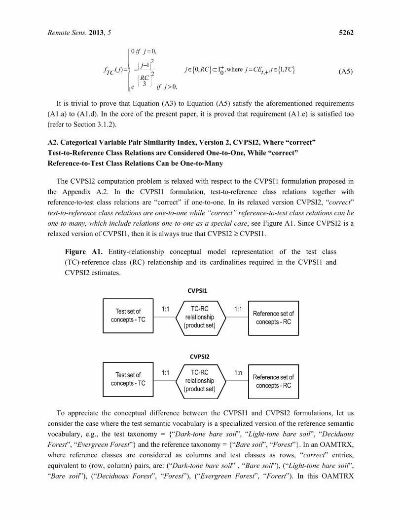
Remote Sens. 2013, 5 5262
{ } { }
0 0,
21
( ) 0, ,where , 1,,02
3 0,
if j
jf j j RC j CE t TCtTC
RCe if j
=
− += ∈ ⊂ Ι = ∈− +
>
(A5)
It is trivial to prove that Equation (A3) to Equation (A5) satisfy the aforementioned requirements
(A1.a) to (A1.d). In the core of the present paper, it is proved that requirement (A1.e) is satisfied too
(refer to Section 3.1.2).
A2. Categorical Variable Pair Similarity Index, Version 2, CVPSI2, Where “correct”
Test-to-Reference Class Relations are Considered One-to-One, While “correct”
Reference-to-Test Class Relations Can be One-to-Many
The CVPSI2 computation problem is relaxed with respect to the CVPSI1 formulation proposed in
the Appendix A.2. In the CVPSI1 formulation, test-to-reference class relations together with
reference-to-test class relations are “correct” if one-to-one. In its relaxed version CVPSI2, “correct”
test-to-reference class relations are one-to-one while “correct” reference-to-test class relations can be
one-to-many, which include relations one-to-one as a special case, see Figure A1. Since CVPSI2 is a
relaxed version of CVPSI1, then it is always true that CVPSI2 ≥ CVPSI1.
Figure A1. Entity-relationship conceptual model representation of the test class
(TC)-reference class (RC) relationship and its cardinalities required in the CVPSI1 and
CVPSI2 estimates.
To appreciate the conceptual difference between the CVPSI1 and CVPSI2 formulations, let us
consider the case where the test semantic vocabulary is a specialized version of the reference semantic
vocabulary, e.g., the test taxonomy = {“Dark-tone bare soil”, “Light-tone bare soil”, “Deciduous
Forest”, “Evergreen Forest”} and the reference taxonomy = {“Bare soil”, “Forest”}. In an OAMTRX,
where reference classes are considered as columns and test classes as rows, “correct” entries,
equivalent to (row, column) pairs, are: (“Dark-tone bare soil” , “Bare soil”), (“Light-tone bare soil”,
“Bare soil”), (“Deciduous Forest”, “Forest”), (“Evergreen Forest”, “Forest”). In this OAMTRX
Test set of concepts - TC
1:1Reference set of
concepts - RC
1:1TC-RC relationship
(product set)
Test set of concepts - TC
1:1Reference set of
concepts - RC
1:nTC-RC relationship
(product set)
CVPSI1
CVPSI2
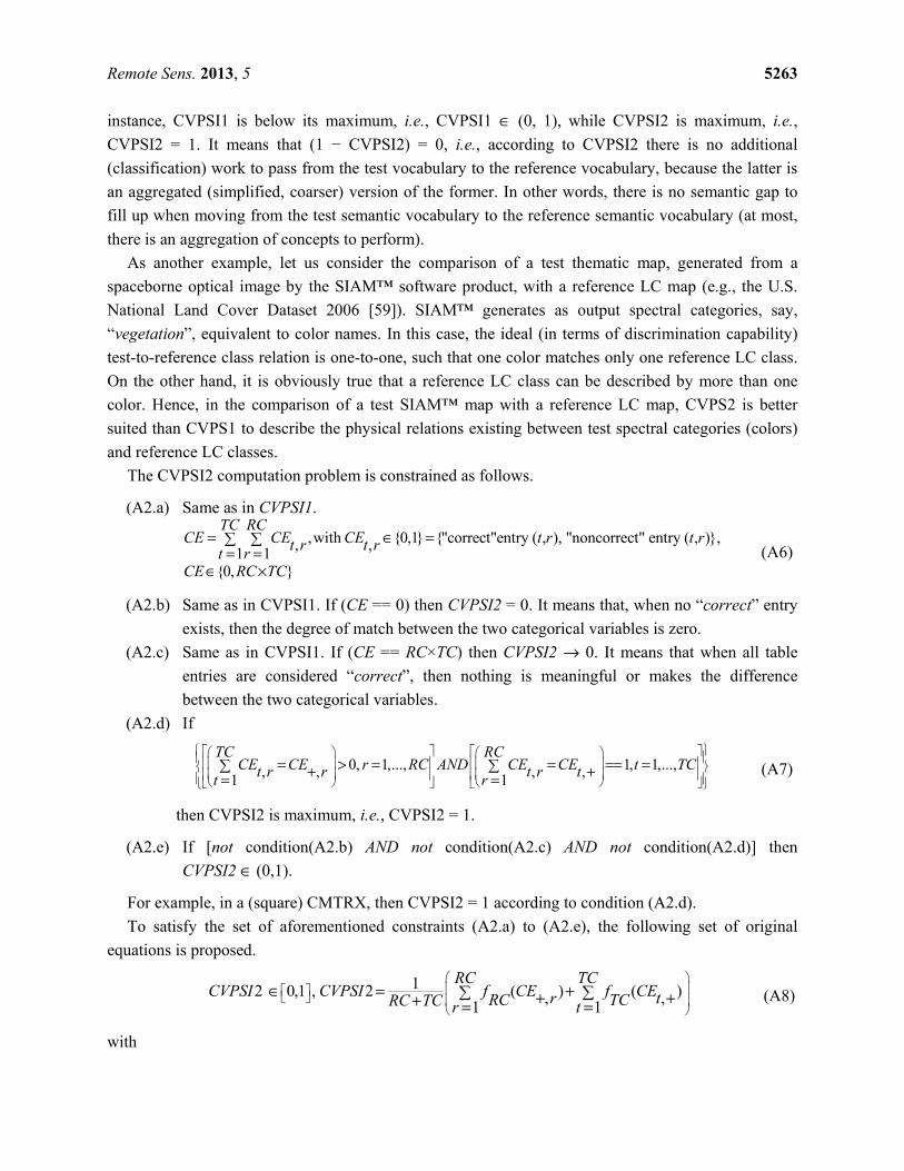
Remote Sens. 2013, 5 5263
instance, CVPSI1 is below its maximum, i.e., CVPSI1 ∈ (0, 1), while CVPSI2 is maximum, i.e.,
CVPSI2 = 1. It means that (1 − CVPSI2) = 0, i.e., according to CVPSI2 there is no additional
(classification) work to pass from the test vocabulary to the reference vocabulary, because the latter is
an aggregated (simplified, coarser) version of the former. In other words, there is no semantic gap to
fill up when moving from the test semantic vocabulary to the reference semantic vocabulary (at most,
there is an aggregation of concepts to perform).
As another example, let us consider the comparison of a test thematic map, generated from a
spaceborne optical image by the SIAM™ software product, with a reference LC map (e.g., the U.S.
National Land Cover Dataset 2006 [59]). SIAM™ generates as output spectral categories, say,
“vegetation”, equivalent to color names. In this case, the ideal (in terms of discrimination capability)
test-to-reference class relation is one-to-one, such that one color matches only one reference LC class.
On the other hand, it is obviously true that a reference LC class can be described by more than one
color. Hence, in the comparison of a test SIAM™ map with a reference LC map, CVPS2 is better
suited than CVPS1 to describe the physical relations existing between test spectral categories (colors)
and reference LC classes.
The CVPSI2 computation problem is constrained as follows.
(A2.a) Same as in CVPSI1.
,with {0,1} {"correct"entry ( , ), "noncorrect" entry ( , )},, ,1 1{0, }
TC RCCE CE CE t r t rt r t rt rCE RC TC
= ∈ = = =
∈ ×
(A6)
(A2.b) Same as in CVPSI1. If (CE == 0) then CVPSI2 = 0. It means that, when no “correct” entry
exists, then the degree of match between the two categorical variables is zero.
(A2.c) Same as in CVPSI1. If (CE == RC×TC) then CVPSI2 → 0. It means that when all table
entries are considered “correct”, then nothing is meaningful or makes the difference
between the two categorical variables.
(A2.d) If
0, 1,..., 1, 1,...,, , , ,1 1
TC RCCE CE r RC AND CE CE t TCt r r t r tt r
= > = = == = + += =
(A7)
then CVPSI2 is maximum, i.e., CVPSI2 = 1.
(A2.e) If [not condition(A2.b) AND not condition(A2.c) AND not condition(A2.d)] then
CVPSI2 ∈ (0,1).
For example, in a (square) CMTRX, then CVPSI2 = 1 according to condition (A2.d).
To satisfy the set of aforementioned constraints (A2.a) to (A2.e), the following set of original
equations is proposed.
12 0,1 , 2 ( ) ( ), ,1 1
RC TCCVPSI CVPSI f CE f CEr tRC TCRC TC r t
∈ = + + ++ = =
(A8)
with
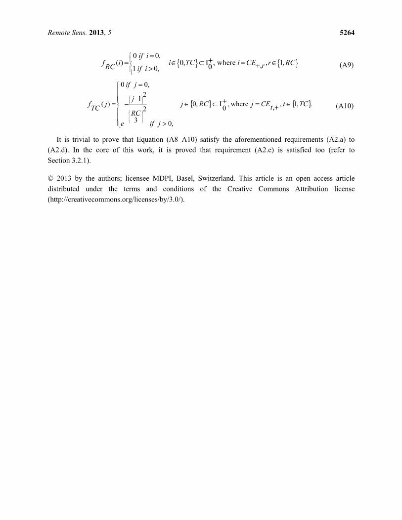
Remote Sens. 2013, 5 5264
{ } { }0 0,
( ) 0, , where , 1,,01 0,
if if i i TC i CE r RCrRC if i
= += ∈ ⊂ Ι = ∈+>
(A9)
{ } { }.,1,,where,0
,0
,0
2
3
21
,00
)( TCttCEjRCj
jif
RC
j
e
jif
jTC
f ∈+=+Ι⊂∈
>
−−
=
=
(A10)
It is trivial to prove that Equation (A8–A10) satisfy the aforementioned requirements (A2.a) to
(A2.d). In the core of this work, it is proved that requirement (A2.e) is satisfied too (refer to
Section 3.2.1).
© 2013 by the authors; licensee MDPI, Basel, Switzerland. This article is an open access article
distributed under the terms and conditions of the Creative Commons Attribution license
(http://creativecommons.org/licenses/by/3.0/).
Related Documents