Public Transit for Special Events: Ridership Prediction ... - arXiv

1

Public Transit for Special Events:Ridership Prediction and Train Optimization

Tejas Santanam, Anthony Trasatti, Pascal Van Hentenryck, and Hanyu ZhangGeorgia Institute of Technology, Atlanta

Abstract—Many special events, including sport games andconcerts, often cause surges in demand and congestion for transitsystems. Therefore, it is important for transit providers to un-derstand their impact on disruptions, delays, and fare revenues.This paper proposes a suite of data-driven techniques that exploitAutomated Fare Collection (AFC) data for evaluating, anticipat-ing, and managing the performance of transit systems duringrecurring congestion peaks due to special events. This includesan extensive analysis of ridership of the two major stadiums indowntown Atlanta using rail data from the Metropolitan AtlantaRapid Transit Authority (MARTA). The paper first highlights theridership predictability at the aggregate level for each station onboth event and non-event days. It then presents an unsupervisedmachine-learning model to cluster passengers and identify whichtrain they are boarding. The model makes it possible to evaluatesystem performance in terms of fundamental metrics such as thepassenger load per train and the wait times of riders. The paperalso presents linear regression and random forest models forpredicting ridership that are used in combination with historicalthroughput analysis to forecast demand. Finally, simulations areperformed that showcase the potential improvements to waittimes and demand matching by leveraging proposed techniquesto optimize train frequencies based on forecasted demand.

Index Terms—Special events, machine learning, public trans-portation, smart cards, and demand forecasting.

I. INTRODUCTION

Special events, including sports games, concerts, and fes-tivals, are important for transit providers; they often lead tofundamentally different ridership patterns and bring significantfare revenues. In addition, special events may be the introduc-tion of certain riders to a transit system, and hence it is criticalto ensure that the system is smooth and efficient, the waitingtimes are reasonable, and the vehicles are not too crowded, inorder to attract additional recurring ridership.

This paper originated as a study of special events for theMetropolitan Atlanta Rapid Transit Authority (MARTA), thetransit system of the city of Atlanta in the state of Georgia. Inparticular, the study aims at addressing two main objectivesof MARTA:

1) Is is possible to forecast special event rail ridershipbased on expected attendance and the type of event usinghistorical Automated Fare Collection (AFC) data;

2) Can optimizing train frequencies based on forecastedridership significantly improve passenger wait times andcongestion following the events?

Tackling these overall objectives requires addressing somesub-objectives to the following questions about special eventridership:

1) How many passengers are using the rail to travel to andfrom special events?

2) Which stations are most popular for event riders?3) What are the passenger loads of the trains?4) How long do riders wait for trains after an event?5) Can special event ridership be predicted?6) Does the incidence of nearby smaller events have an

impact on ridership to larger special events?To answer these questions, the paper presents a suite of

data-driven methods that leverage Automated Fare Collection(AFC). It demonstrates that the data-driven tools answerthe above questions on sporting events located at the twodowntown stadiums, the Mercedes-Benz Stadium and the StateFarm Arena which host the Atlanta Hawks, Atlanta Falcons,and Atlanta United. From a high level perspective, this paperproposes the following methodology for MARTA, and possiblyother transit agencies:

1) Obtain an attendance prediction from stadium ticket salesand predict ridership from that attendance using super-vised machine learning;

2) Using historical trends, estimate the arrival times ofpassengers to the stations near the stadium;

3) Based on the forecasted arrivals, optimize the train fre-quencies to minimize waiting times, maximize safety, andminimize costs.

To develop this methodology, the paper makes the followingtechnical and analytical contributions.

1) The paper introduces station signatures to highlight theridership consistency at the aggregate level for the base-line (non-event) days and post-games event peaks. Theseconsistencies provide a foundation to estimate special-event ridership accurately and answer the above ques-tions.

2) The paper combines station signatures with origin-destination (OD) pairs to highlight the strong correlationbetween the origins of special-event ridership and parkinglocations.

3) The paper uses unsupervised learning and simulation toestimate the train loads, departure times, and the asso-ciated waiting times of the riders. These estimates werevalidated with a simulation model for train boardings,inferring the train occupancy.

4) The paper uses supervised learning to predict ridershipwith high accuracy, giving planners the tools to optimizetrain schedules for future events. The paper describesthe performance of three predictive models: a linear

arX

iv:2

106.

0535

9v1

[m

ath.

OC

] 9

Jun

202

1

2

regression, a random forest, and a combination of linearregression and random forest, where the random forestpredicts the residual errors of the linear regression.

5) The paper demonstrates that optimizing the train fre-quencies based on the forecasted demand may improvewait times and significantly reduce the number of ridersleft behind during post-game peaks while using a similarnumber of trains.

The rest of the paper is organized as follows. Section IIreviews prior work on similar topics. Section III presents thecase study. Section IV presents the analysis of the baselineridership and the signatures for entries and exits at rail stationson weekdays and weekends. It also analyzes the specialevent ridership and estimates how many riders use the railto travel to and from the events and where they come from.Section V applies unsupervised learning to cluster riders andpredict which train they board, their waiting times, as wellas the departure times of the trains. Section VI presentssimple supervised learning models to predict the ridership forvarious types of recurring special events that can be used withhistorical trends to forecast arrivals at nearby stations afterthe game. This section demonstrates how optimizing the trainfrequencies based on this forecasted demand may significantlyimprove the post-game congestion and wait times. This sectionalso addresses the question of how nearby smaller events affectthe ridership to larger events.

II. LITERATURE REVIEW

Automated Fare Collection (AFC) technologies have en-abled more sophisticated analysis of transit ridership [1], [2].Various data sources have been used to study special-event rid-ership including survey, AFC, and web data [3], [4]. Rodrigueset al. (2017) use a Bayesian additive model to understand andpredict event riders arriving by public transit using Singaporesmart card data [5]. That model creates a separate predictionfor each different event and baseline ridership using 5 monthsof data, grouping arrivals in 30 minute bins. Karnberger et al.(2020) look at the Munich public transit system, also usingsome AFC data. They look at weekly system averages andbuild a gradient boosted random forest prediction system forridership between linked stations in parts of Munich [6]. Thetype of day (holiday, weekend, etc.) and the existence of a fewtypes of events are used as inputs to the model which focuseson link-level riders.

Other papers looked at prediction of sporting event atten-dees. Ni et al. (2017) establish a correlation between tweetsrelated to an event and event ridership flow. The paper builds alinear regression model to predict ridership from the number oftweets for Mets games and US Open tennis matches [7]. King(2017) predicts NBA game attendance using random forestmodels, but the ridership and travel modes are not considered[8].

Short-term prediction has also been the focus of otherridership models, which contrasts to the longer time horizonconsidered in this paper. Li et al. (2017) use a multiscale radialbasis function network to predict rail ridership at three largeBeijing rail stations. The model predicts riders at a station halfan hour in the future using a one-step-ahead model [9].

Fig. 1: The MARTA Rail Lines and Stations

Begin Date Category Event Location Attendance01/15/201815:00:00 Basketball - Hawks Hawks v San Antonio Spurs State Farm Arena 15,000

01/16/201807:00:00 Conference Mary Kay Leadership Conference

Georgia WorldCongress Center 7,000

01/16/201809:00:00 AmericasMart Intnl Gift & Home Furnishings AmericasMart 72,000

TABLE I: Event Data Example

III. THE CASE STUDY

A. Map of MARTA Rail System

Figure 1 depicts the four MARTA rail lines [10]. The Redand Gold lines run North-South and the Blue and Green linesrun East-West, with the two directions intersecting at FivePoints. The three event locations considered in this paper are

1) The Mercedes-Benz Stadium;2) The State Farm Arena;3) The Georgia World Congress Center.

These three key venues located in downtown Atlanta on theBlue and Green lines are highlighted in the left center of themap. The two closest stops are Dome/GWCC and Vine City.Users coming from the North or South can use the Red orGold line and transfer at Five Points to get on the Blue orGreen line. These locations are important for the subsequentanalyses.

B. Event Data

The event data provided by MARTA is a list of many publicevents in the Atlanta area during 2018 and 2019 containing

1) the type of Event;2) the location;3) the date;4) the time;5) the estimated attendance.

An example of event entries is presented in Table I.The three most popular venues for large events in Atlanta

are the Georgia World Congress Center, the Mercedes BenzStadium (MBS), and the State Farm Arena, which werementioned earlier as the focus of this paper. In 2018 and 2019,

3

Primary Event # of Days Avg. Attendance Avg. Post-GameRidership

Basketball -Hawks 67 15,278 1,425Football Games 28 69,477 10,846

Soccer 39 52,712 8,037

Day Type # of DaysAvg. Attendanceof Primary Event

Avg. Post-GameRidership

Single Event 78 38,062 5,487Two Events 56 36,712 5,082

TABLE II: The Event Data Overview.

UserId TransactionDT UseType Station101 2018/3/20 8:01 Entry (Tag On) Doraville101 2018/3/20 8:28 Exit (Tag Off) Lindbergh Center101 2018/3/20 20:05 Entry (Tag On) Lindbergh Center101 2018/3/20 20:21 Exit (Tag Off) Doraville

TABLE III: An example of AFC rail data.

UserId EntryDT EntryStation ExitDT ExitStation101 3/20/18 8:01 Doraville 3/20/18 8:28 Lindbergh101 3/20/18 20:05 Lindbergh 3/20/18 20:21 Doraville

TABLE IV: An example of chained AFC Rail data.

there were 1330 special events with an estimated attendancegreater than 500 people in Atlanta. 706 of these 1330 specialevemts were held in the Georgia World Congress Center, theMercedes Benz Stadium (MBS), or the State Farm Arena.The three locations are geographically close to each other;moreover, the closest two rail stations are the Dome/GWCCand Vine City stations.

This paper focuses on events with the largest impact and,in particular, the 200 sporting events (Basketball, Soccer, andFootball games). All basketball games were held in the StateFarm Arena, while the soccer and football games were heldin the MBS. Apart from the sporting events, there were 74conferences, 53 conventions, and 102 expos & shows at thetarget locations. However, these events generally have smallerattendances, and riders leave these events in patterns that arefundamentally different from sporting events. In many cases,people go in and out of the events throughout the day, leadingto a ridership more dissipated over a larger time horizon.Overall, these events have a smaller impact on the congestionof the rail system. These factors, as well as low sample sizes,make longer-term events like conventions and conferencespoor subjects for analysis. The event data is summarized inTable II.

C. Automated Fare Collection Data

To enter or exit the MARTA rail system, customers arerequired to use a ticket or a reloadable card (the “BreezeCard”) at the gates of individual stations. MARTA providedanonymized transaction-level data showing tap-in and tap-outtimes and locations for the rail network from 2016 to mid-2020. Example entries of Breeze Card data are shown in TableIII.

Trip chaining is performed to turn these individual trans-actions into Origin-Destination (OD) pairs. Tap-ins and tap-outs, when chained, are sufficient to determine where a rider

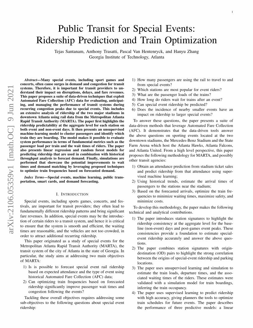
Fig. 2: Monthly Baseline Signatures for Entries at North Ave RailStation

enters and exits the rail network. For the most part, entries arematched to the following exit and create an OD pair. Table IVshows an example of the chained trips after they are processed.In some cases, the chained trip is an entry and exit at the samestation back to back. For example, when an exit tap occurs, butthere is a missing entry tap, then the system records a “forcedentry” transaction and an exit transaction at the exit station atthe same time. Similarly, if someone tries to re-enter a station,but there is a missing exit transaction or an extended amount ofperiod has elapsed (3-4 hours), the system will add a “forcedexit” transaction at the most recent tap-in location. Since themajority of transactions follow the expected pattern (pairs ofdistinct locations), the analysis focuses on these transactions.

IV. RIDERSHIP ANALYSIS

This section first analyzes ridership on baseline (non-event)days, as average day patterns help identify the effects of spe-cial events on the system. The analysis considers baseline daysand creates individual ridership signatures for each station.These signatures are then used to calculate the ridership thatcan be attributed to special events. The analysis also assessesthe consistency of special-event ridership.

A. Station Signatures

To create representative signatures for baseline days, thetransaction data is to partition on the basis of• weekday versus weekend;• entry versus exit• event day versus baseline day.

This partitioned data is used to create four baseline signaturesfor each station: weekday entry, weekday exit, weekend entry,and weekend exit. Since the rail is closed between 1:30amand 4:30am, the day is defined as the 24-hour period startingat 3AM and finishing 3AM to capture riders returning aftermidnight. Each day is further partitioned into 15 minuteintervals and the number of riders are counted for each intervalfor each of the four types of transactions.

4

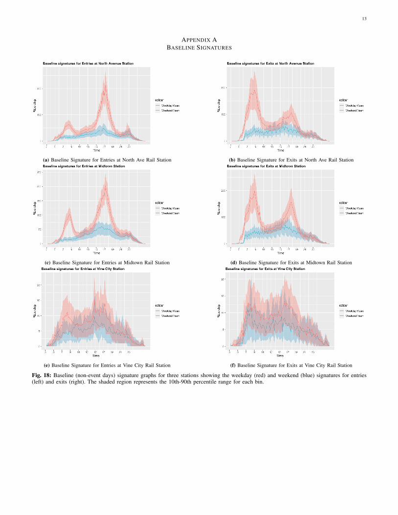
Figure 2 shows how the signatures are very similar andconsistent month-to-month. This kind of consistency is goodfor future modeling and planning. In the appendix, Figures18a–18d depict the four baseline signatures for the NorthAvenue and Midtown stations. The shaded region representsthe 10th-90th percentile range for each bin. The signaturesshow regular commute spikes on weekdays for both entryand exit signatures. They also show that riders follow similarpatterns throughout the year. Figures 18e–18f report the resultsfor the Vine City station, which does not have many regularcommuters. There is still a weekday and weekend differencefor the ridership of Vine City station, but the overall magnitudeof ridership is low compared to the North Avenue and Mid-town stations. As will become clear, this low ridership changesdrastically in presence of an event as it is one of two closeststations to the nearby Mercedes-Benz Stadium and State FarmArena.

B. Event Ridership Estimation

The last section highlights the consistency of the baselineridership. Pereira et al. measures and detects hotspots bycounting the number of riders greater than the median, wherethe curve exceeds the baseline’s 90th percentile [11]. Thissection uses this same technique to measure the special eventridership. This analysis focuses on riders with an origin ordestination at the Dome/GWCC and Vine City stations, sincethe majority of riders use these two stations to get to and fromthe events at the three venues of focus. This measurement isformalized as follows. Let• rb(t) be the baseline ridership at time t;• r+b (t) be the 90th percentile of the baseline;• re(t) be the actual ridership during the event at time t;• ts be the earliest time with re(t) > r+b (t) to capture the

start of the event ridership;• te be the latest time with re(t) > r+b (t) to capture the

end of the event ridership;• ra(t) be the number of rail riders at time t who attended

the event;The number of rail riders who attend the event at time t isgiven by

ra(t) = re(t)− rb(t)1(re(t) > r+b (t)) (1)

and the number of rail riders attending the event is given by

Ta =∑

∀t∈[ts,te]

ra(t). (2)

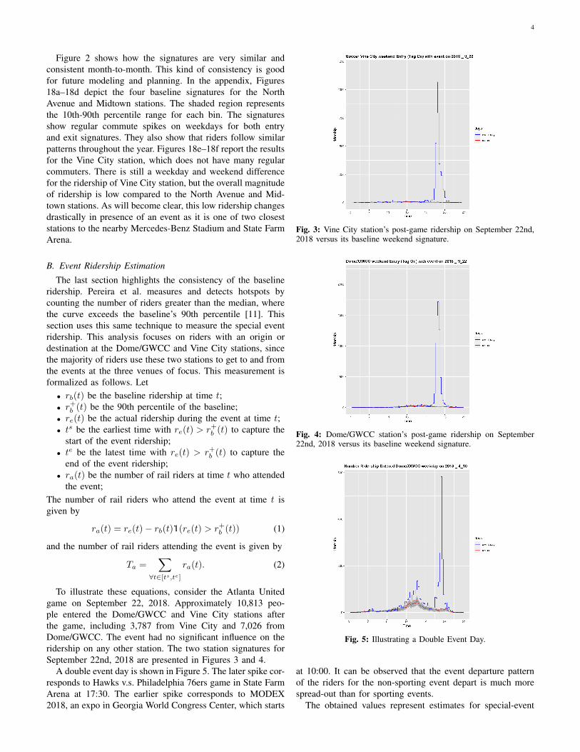
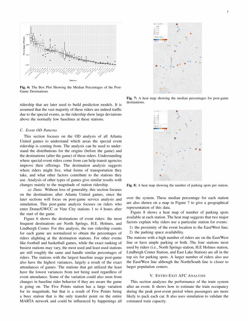
To illustrate these equations, consider the Atlanta Unitedgame on September 22, 2018. Approximately 10,813 peo-ple entered the Dome/GWCC and Vine City stations afterthe game, including 3,787 from Vine City and 7,026 fromDome/GWCC. The event had no significant influence on theridership on any other station. The two station signatures forSeptember 22nd, 2018 are presented in Figures 3 and 4.

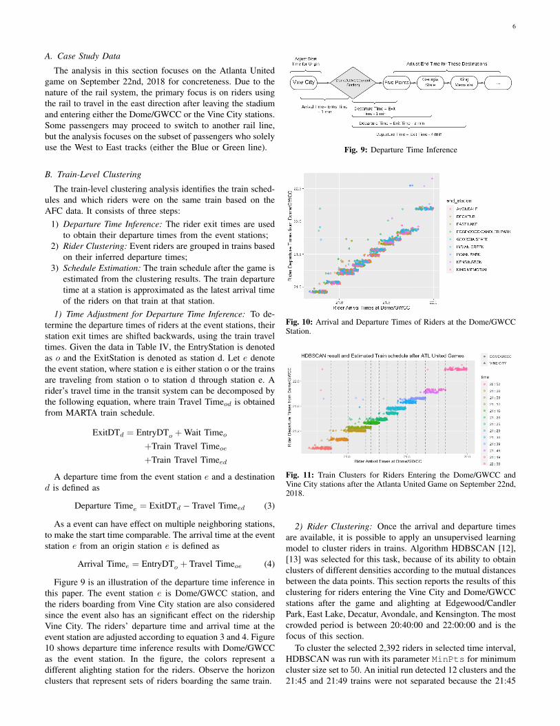
A double event day is shown in Figure 5. The later spike cor-responds to Hawks v.s. Philadelphia 76ers game in State FarmArena at 17:30. The earlier spike corresponds to MODEX2018, an expo in Georgia World Congress Center, which starts

Fig. 3: Vine City station’s post-game ridership on September 22nd,2018 versus its baseline weekend signature.

Fig. 4: Dome/GWCC station’s post-game ridership on September22nd, 2018 versus its baseline weekend signature.

Fig. 5: Illustrating a Double Event Day.

at 10:00. It can be observed that the event departure patternof the riders for the non-sporting event depart is much morespread-out than for sporting events.

The obtained values represent estimates for special-event

5

Fig. 6: The Box Plot Showing the Median Percentages of the Post-Game Destinations

ridership that are later used to build prediction models. It isassumed that the vast majority of these riders are indeed trafficdue to the special events, as the ridership show large deviationsabove the normally low baselines at these stations.

C. Event OD Patterns

This section focuses on the OD analysis of all AtlantaUnited games to understand which areas the special eventridership is coming from. The analysis can be used to under-stand the distributions for the origins (before the game) andthe destinations (after the game) of these riders. Understandingwhere special-event riders come from can help transit agenciesimprove their offerings. The destination analysis suggestswhere riders might live, what forms of transportation theytake, and what other factors contribute to the stations theyuse. Analysis of other types of games give similar results withchanges mainly to the magnitude of station ridership.

a) Data: Without loss of generality, this section focuseson the destinations after Atlanta United games, since thelater sections will focus on post-game service analysis andsimulation. This post-game analysis focuses on riders whoenter Dome/GWCC or Vine City stations 1 to 4 hours afterthe start of the game.

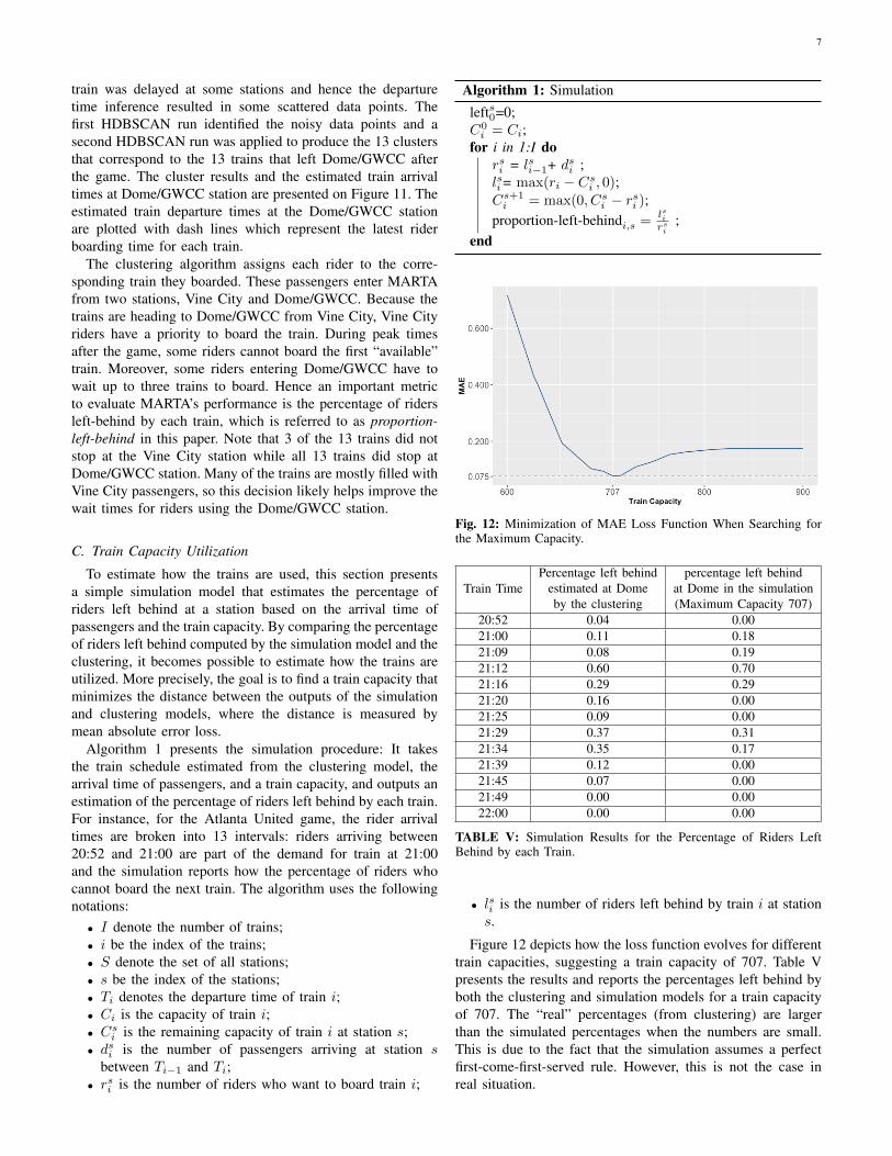
Figure 6 shows the destinations of event riders: the mostfrequent destinations are North Springs, H.E. Holmes, andLindbergh Center. For this analysis, the raw ridership countsfor each game are normalized to obtain the percentages ofriders alighting at the destination stations. For other eventslike football and basketball games, while the exact ranking ofbusiest stations may vary, the most used and least used stationsare still roughly the same and handle similar percentages ofriders. The stations with the largest baseline usage post-gamealso have the highest variances, largely a result of the exactattendances of games. The stations that get utilized the leasthave the lowest variances from not being used regardless ofevent attendance. Some of the variation could also stem fromchanges in baseline rider behavior if they are aware the gameis going on. The Five Points station has a large variationfor its magnitude, but that is a result of Five Points beinga busy station that is the only transfer point on the entireMARTA network and could be influenced by happenings all

Fig. 7: A heat map showing the median percentages for post-gamedestinations.

Fig. 8: A heat map showing the number of parking spots per station.

over the system. These median percentage for each stationare also shown on a map in Figure 7 to give a geographicalrepresentation of this data.

Figure 8 shows a heat map of number of parking spotsavailable at each station. The heat map suggests that two majorfactors explain why riders use a particular station for events:

1) the proximity of the event location to the East/West line;2) the parking space availability.

The stations with a high number of riders are on the East/Westline or have ample parking or both. The four stations mostused by riders (i.e., North Springs station, H.E Holmes station,Lindbergh Center Station, and East Lake Station) are all in thetop six for parking spots. A larger number of riders also usethe East/West line although the North/South line is closer tolarger population centers.

V. ENTRY-EXIT AFC ANALYSIS

This section analyzes the performance of the train systemafter an event. It shows how to estimate the train occupancyduring the peak post-event period when passengers are morelikely to pack each car. It also uses simulation to validate theestimated train capacity.

6

A. Case Study Data

The analysis in this section focuses on the Atlanta Unitedgame on September 22nd, 2018 for concreteness. Due to thenature of the rail system, the primary focus is on riders usingthe rail to travel in the east direction after leaving the stadiumand entering either the Dome/GWCC or the Vine City stations.Some passengers may proceed to switch to another rail line,but the analysis focuses on the subset of passengers who solelyuse the West to East tracks (either the Blue or Green line).

B. Train-Level Clustering

The train-level clustering analysis identifies the train sched-ules and which riders were on the same train based on theAFC data. It consists of three steps:

1) Departure Time Inference: The rider exit times are usedto obtain their departure times from the event stations;

2) Rider Clustering: Event riders are grouped in trains basedon their inferred departure times;

3) Schedule Estimation: The train schedule after the game isestimated from the clustering results. The train departuretime at a station is approximated as the latest arrival timeof the riders on that train at that station.

1) Time Adjustment for Departure Time Inference: To de-termine the departure times of riders at the event stations, theirstation exit times are shifted backwards, using the train traveltimes. Given the data in Table IV, the EntryStation is denotedas o and the ExitStation is denoted as station d. Let e denotethe event station, where station e is either station o or the trainsare traveling from station o to station d through station e. Arider’s travel time in the transit system can be decomposed bythe following equation, where train Travel Timeod is obtainedfrom MARTA train schedule.

ExitDTd = EntryDTo + Wait Timeo+Train Travel Timeoe+Train Travel Timeed

A departure time from the event station e and a destinationd is defined as

Departure Timee = ExitDTd − Travel Timeed (3)

As a event can have effect on multiple neighboring stations,to make the start time comparable. The arrival time at the eventstation e from an origin station e is defined as

Arrival Timee = EntryDTo + Travel Timeoe (4)

Figure 9 is an illustration of the departure time inference inthis paper. The event station e is Dome/GWCC station, andthe riders boarding from Vine City station are also consideredsince the event also has an significant effect on the ridershipVine City. The riders’ departure time and arrival time at theevent station are adjusted according to equation 3 and 4. Figure10 shows departure time inference results with Dome/GWCCas the event station. In the figure, the colors represent adifferent alighting station for the riders. Observe the horizonclusters that represent sets of riders boarding the same train.

Fig. 9: Departure Time Inference

Fig. 10: Arrival and Departure Times of Riders at the Dome/GWCCStation.

Fig. 11: Train Clusters for Riders Entering the Dome/GWCC andVine City stations after the Atlanta United Game on September 22nd,2018.

2) Rider Clustering: Once the arrival and departure timesare available, it is possible to apply an unsupervised learningmodel to cluster riders in trains. Algorithm HDBSCAN [12],[13] was selected for this task, because of its ability to obtainclusters of different densities according to the mutual distancesbetween the data points. This section reports the results of thisclustering for riders entering the Vine City and Dome/GWCCstations after the game and alighting at Edgewood/CandlerPark, East Lake, Decatur, Avondale, and Kensington. The mostcrowded period is between 20:40:00 and 22:00:00 and is thefocus of this section.

To cluster the selected 2,392 riders in selected time interval,HDBSCAN was run with its parameter MinPts for minimumcluster size set to 50. An initial run detected 12 clusters and the21:45 and 21:49 trains were not separated because the 21:45

7

train was delayed at some stations and hence the departuretime inference resulted in some scattered data points. Thefirst HDBSCAN run identified the noisy data points and asecond HDBSCAN run was applied to produce the 13 clustersthat correspond to the 13 trains that left Dome/GWCC afterthe game. The cluster results and the estimated train arrivaltimes at Dome/GWCC station are presented on Figure 11. Theestimated train departure times at the Dome/GWCC stationare plotted with dash lines which represent the latest riderboarding time for each train.

The clustering algorithm assigns each rider to the corre-sponding train they boarded. These passengers enter MARTAfrom two stations, Vine City and Dome/GWCC. Because thetrains are heading to Dome/GWCC from Vine City, Vine Cityriders have a priority to board the train. During peak timesafter the game, some riders cannot board the first “available”train. Moreover, some riders entering Dome/GWCC have towait up to three trains to board. Hence an important metricto evaluate MARTA’s performance is the percentage of ridersleft-behind by each train, which is referred to as proportion-left-behind in this paper. Note that 3 of the 13 trains did notstop at the Vine City station while all 13 trains did stop atDome/GWCC station. Many of the trains are mostly filled withVine City passengers, so this decision likely helps improve thewait times for riders using the Dome/GWCC station.

C. Train Capacity Utilization

To estimate how the trains are used, this section presentsa simple simulation model that estimates the percentage ofriders left behind at a station based on the arrival time ofpassengers and the train capacity. By comparing the percentageof riders left behind computed by the simulation model and theclustering, it becomes possible to estimate how the trains areutilized. More precisely, the goal is to find a train capacity thatminimizes the distance between the outputs of the simulationand clustering models, where the distance is measured bymean absolute error loss.

Algorithm 1 presents the simulation procedure: It takesthe train schedule estimated from the clustering model, thearrival time of passengers, and a train capacity, and outputs anestimation of the percentage of riders left behind by each train.For instance, for the Atlanta United game, the rider arrivaltimes are broken into 13 intervals: riders arriving between20:52 and 21:00 are part of the demand for train at 21:00and the simulation reports how the percentage of riders whocannot board the next train. The algorithm uses the followingnotations:• I denote the number of trains;• i be the index of the trains;• S denote the set of all stations;• s be the index of the stations;• Ti denotes the departure time of train i;• Ci is the capacity of train i;• Cs

i is the remaining capacity of train i at station s;• dsi is the number of passengers arriving at station s

between Ti−1 and Ti;• rsi is the number of riders who want to board train i;

Algorithm 1: Simulation

lefts0=0;C0

i = Ci;for i in 1:I do

rsi = lsi−1+ dsi ;lsi = max(ri − Cs

i , 0);Cs+1

i = max(0, Csi − rsi );

proportion-left-behindi,s =lsirsi

;end

Fig. 12: Minimization of MAE Loss Function When Searching forthe Maximum Capacity.

Train TimePercentage left behind

estimated at Domeby the clustering

percentage left behindat Dome in the simulation(Maximum Capacity 707)

20:52 0.04 0.0021:00 0.11 0.1821:09 0.08 0.1921:12 0.60 0.7021:16 0.29 0.2921:20 0.16 0.0021:25 0.09 0.0021:29 0.37 0.3121:34 0.35 0.1721:39 0.12 0.0021:45 0.07 0.0021:49 0.00 0.0022:00 0.00 0.00

TABLE V: Simulation Results for the Percentage of Riders LeftBehind by each Train.

• lsi is the number of riders left behind by train i at stations.

Figure 12 depicts how the loss function evolves for differenttrain capacities, suggesting a train capacity of 707. Table Vpresents the results and reports the percentages left behind byboth the clustering and simulation models for a train capacityof 707. The “real” percentages (from clustering) are largerthan the simulated percentages when the numbers are small.This is due to the fact that the simulation assumes a perfectfirst-come-first-served rule. However, this is not the case inreal situation.

8

The maximum capacity of 707 is a lower bound estimationbecause riders already on the trains (approximately a totalof 35 people for the whole time period) are not countedhere. These trains are 6-car trains post-game which have arecommended maximum capacity of 576 people. From thisanalysis, however, one can see that the maximum capacityis often exceeded post-game: people often cram together invery close quarters as a result. It is also likely that this over-capacity situation leads to an increased risk of accident, injury,or illness. However, the analysis simply confirms the anecdotalevidence that people have a tendency to “pack it in” aftersporting events. Note also that, under the assumption thatpeople left behind end up boarding the next train before thenew arrivals, riders wait a maximum of two trains, whichcorresponds to the case in Figure 11.

VI. PREDICTIVE ANALYTICS

The end of a special event can lead to a large surge ofpassengers flooding to public transit. This can lead to crowdingin the stations and extended wait times. The train operatorsadjust the normal schedule by pulling reserve trains “out-of-pocket” in order to match the increased demand. Trainoperators have an important job of being aware of the stateof the game, so that they can adjust the actual scheduleaccordingly. The goal of this section is to see if the proposedpredictive analytics may be able to help train operators bebetter prepared for these recurring post-game demand spikes.

To optimize the train schedules of future events, it remainsto demonstrate that the ridership can be predicted with highaccuracy. This section shows that this is indeed possible. Itfirst shows the consistency of station arrivals after a game. Itthen shows how to predict total ridership with high accuracy.Finally, these two results are leveraged as a demand forecast.The proposed train schedules designed using the forecasteddemand are compared through simulation to the actual trainschedules against the post-game arrival data. The proposedtrain schedules reduce the number of riders left behind andwaiting times of the riders during post-game peaks.

A. Throughput Consistency

This section highlights the post-game throughput consis-tency for special events. Due to their larger sizes, events atMercedes-Benz where the upper-deck seating was open arethe focus of this section. In games with an open upper deck,an additional 30,000 seats are available for purchase in theupper deck of Mercedes-Benz Stadium. Due to the additionalattendance, these events have a much larger impact on theMARTA rail system, especially compared to Atlanta Hawksgames where the average attendance is only 15,000 people.In this section, the post-game throughput is analyzed from 40minutes before the end time to 80 minutes after the end time.

In most games, it is assumed that the end time is theaverage game length after the scheduled start time: 1 hour &50 minutes for soccer and 3 hours & 10 minutes for football.However, a few of the end times were adjusted in this analysisbecause it was believed that the end time might have beendelayed due to injuries, delayed starts, or overtime. The delay

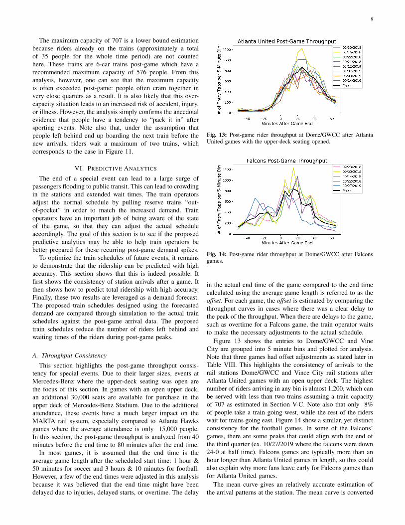
Fig. 13: Post-game rider throughput at Dome/GWCC after AtlantaUnited games with the upper-deck seating opened.

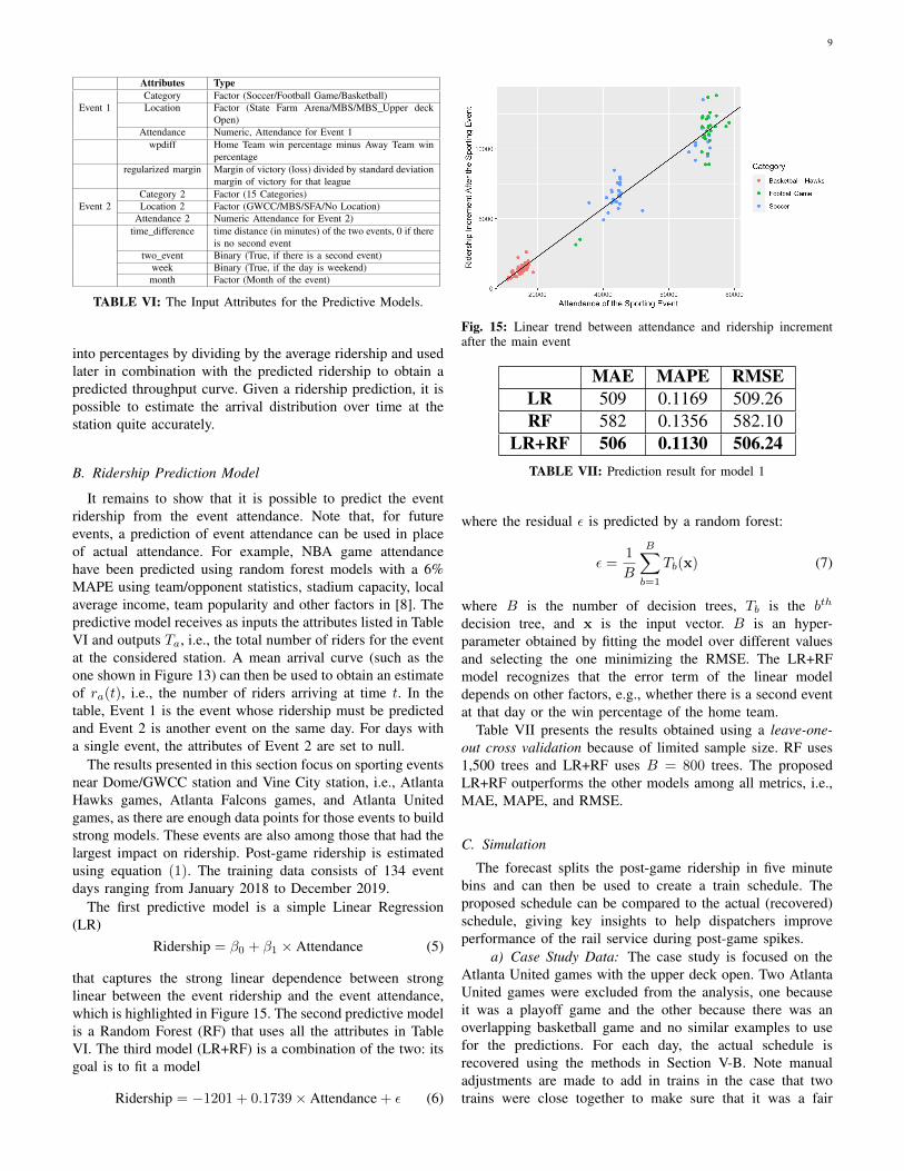
Fig. 14: Post-game rider throughput at Dome/GWCC after Falconsgames.

in the actual end time of the game compared to the end timecalculated using the average game length is referred to as theoffset. For each game, the offset is estimated by comparing thethroughput curves in cases where there was a clear delay tothe peak of the throughput. When there are delays to the game,such as overtime for a Falcons game, the train operator waitsto make the necessary adjustments to the actual schedule.

Figure 13 shows the entries to Dome/GWCC and VineCity are grouped into 5 minute bins and plotted for analysis.Note that three games had offset adjustments as stated later inTable VIII. This highlights the consistency of arrivals to therail stations Dome/GWCC and Vince City rail stations afterAtlanta United games with an open upper deck. The highestnumber of riders arriving in any bin is almost 1,200, which canbe served with less than two trains assuming a train capacityof 707 as estimated in Section V-C. Note also that only 8%of people take a train going west, while the rest of the riderswait for trains going east. Figure 14 show a similar, yet distinctconsistency for the football games. In some of the Falcons’games, there are some peaks that could align with the end ofthe third quarter (ex. 10/27/2019 where the falcons were down24-0 at half time). Falcons games are typically more than anhour longer than Atlanta United games in length, so this couldalso explain why more fans leave early for Falcons games thanfor Atlanta United games.

The mean curve gives an relatively accurate estimation ofthe arrival patterns at the station. The mean curve is converted

9

Attributes Type

Event 1Category Factor (Soccer/Football Game/Basketball)Location Factor (State Farm Arena/MBS/MBS Upper deck

Open)Attendance Numeric, Attendance for Event 1

wpdiff Home Team win percentage minus Away Team winpercentage

regularized margin Margin of victory (loss) divided by standard deviationmargin of victory for that league

Event 2Category 2 Factor (15 Categories)Location 2 Factor (GWCC/MBS/SFA/No Location)

Attendance 2 Numeric Attendance for Event 2)time difference time distance (in minutes) of the two events, 0 if there

is no second eventtwo event Binary (True, if there is a second event)

week Binary (True, if the day is weekend)month Factor (Month of the event)

TABLE VI: The Input Attributes for the Predictive Models.

into percentages by dividing by the average ridership and usedlater in combination with the predicted ridership to obtain apredicted throughput curve. Given a ridership prediction, it ispossible to estimate the arrival distribution over time at thestation quite accurately.

B. Ridership Prediction Model

It remains to show that it is possible to predict the eventridership from the event attendance. Note that, for futureevents, a prediction of event attendance can be used in placeof actual attendance. For example, NBA game attendancehave been predicted using random forest models with a 6%MAPE using team/opponent statistics, stadium capacity, localaverage income, team popularity and other factors in [8]. Thepredictive model receives as inputs the attributes listed in TableVI and outputs Ta, i.e., the total number of riders for the eventat the considered station. A mean arrival curve (such as theone shown in Figure 13) can then be used to obtain an estimateof ra(t), i.e., the number of riders arriving at time t. In thetable, Event 1 is the event whose ridership must be predictedand Event 2 is another event on the same day. For days witha single event, the attributes of Event 2 are set to null.

The results presented in this section focus on sporting eventsnear Dome/GWCC station and Vine City station, i.e., AtlantaHawks games, Atlanta Falcons games, and Atlanta Unitedgames, as there are enough data points for those events to buildstrong models. These events are also among those that had thelargest impact on ridership. Post-game ridership is estimatedusing equation (1). The training data consists of 134 eventdays ranging from January 2018 to December 2019.

The first predictive model is a simple Linear Regression(LR)

Ridership = β0 + β1 × Attendance (5)

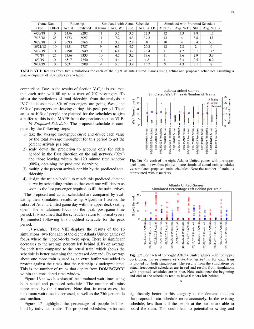
that captures the strong linear dependence between stronglinear between the event ridership and the event attendance,which is highlighted in Figure 15. The second predictive modelis a Random Forest (RF) that uses all the attributes in TableVI. The third model (LR+RF) is a combination of the two: itsgoal is to fit a model

Ridership = −1201 + 0.1739× Attendance + ε (6)

Fig. 15: Linear trend between attendance and ridership incrementafter the main event

MAE MAPE RMSELR 509 0.1169 509.26RF 582 0.1356 582.10

LR+RF 506 0.1130 506.24TABLE VII: Prediction result for model 1

where the residual ε is predicted by a random forest:

ε =1

B

B∑b=1

Tb(x) (7)

where B is the number of decision trees, Tb is the bth

decision tree, and x is the input vector. B is an hyper-parameter obtained by fitting the model over different valuesand selecting the one minimizing the RMSE. The LR+RFmodel recognizes that the error term of the linear modeldepends on other factors, e.g., whether there is a second eventat that day or the win percentage of the home team.

Table VII presents the results obtained using a leave-one-out cross validation because of limited sample size. RF uses1,500 trees and LR+RF uses B = 800 trees. The proposedLR+RF outperforms the other models among all metrics, i.e.,MAE, MAPE, and RMSE.

C. Simulation

The forecast splits the post-game ridership in five minutebins and can then be used to create a train schedule. Theproposed schedule can be compared to the actual (recovered)schedule, giving key insights to help dispatchers improveperformance of the rail service during post-game spikes.

a) Case Study Data: The case study is focused on theAtlanta United games with the upper deck open. Two AtlantaUnited games were excluded from the analysis, one becauseit was a playoff game and the other because there was anoverlapping basketball game and no similar examples to usefor the predictions. For each day, the actual schedule isrecovered using the methods in Section V-B. Note manualadjustments are made to add in trains in the case that twotrains were close together to make sure that it was a fair

10

Game Data Ridership Simulated with Actual Schedule Simulated with Proposed ScheduleDate Offset Actual Predicted # trains Avg. WT Std. Avg. % LB # trains Avg. WT Std. Avg. % LB

6/30/18 0 7456 8292 11 5.7 3.5 22.3 12 3.3 2.8 1.27/15/18 25 8773 8097 11 7.2 4.3 39.2 12 4 3.8 129/22/18 0 7693 6765 11 3.8 2.8 8 10 4 3.4 5.3

10/21/18 10 6431 7787 9 6.5 4.7 20.2 12 2.8 2 05/12/19 0 7790 6949 11 6.1 3.7 28.4 11 4.2 3.1 13.57/7/19 25 7356 7333 10 4.7 3.2 13.6 11 3.6 2.9 3.38/3/19 0 6517 7250 10 4.4 3.4 4.8 11 3.3 2.5 0.29/14/19 0 6631 5909 9 5.3 3.9 15.7 9 4.3 3.1 8

TABLE VIII: Results from two simulations for each of the eight Atlanta United Games using actual and proposed schedules assuming amax occupancy of 707 riders per vehicle.

comparison. Due to the results of Section V-C, it is assumedthat each train will fill up to a max of 707 passengers. Toadjust the predictions of total ridership, from the analysis inIV-C, it is assumed 8% of passengers are going West, and68% of passengers are leaving during this peak period. Then,an extra 10% of people are planned for the schedules to givea buffer as this is the MAPE from the previous section VI-B.

b) Proposed Schedule: The proposed schedule is com-puted by the following steps:

1) take the average throughput curve and divide each valueby the total average throughput for this period to get thepercent arrivals per bin;

2) scale down the prediction to account only for ridersheaded in the East direction on the rail network (92%)and those leaving within the 120 minute time window(68%), obtaining the predicted ridership;

3) multiply the percent arrivals per bin by the predicted totalridership;

4) design the train schedule to match this predicted demandcurve by scheduling trains so that each one will depart assoon as the last passenger required to fill the train arrives.

The proposed and actual scheduled are compared by eval-uating their simulation results using Algorithm 1 across thesubset of Atlanta United game day with the upper deck seatingopen. The simulations focus on the peak post-game timeperiod. It is assumed that the schedules return to normal (every10 minutes) following this modified schedule for the peakperiod.

c) Results: Table VIII displays the results of the 16simulations: two for each of the eight Atlanta United games offocus where the upper-decks were open. There is significantdecreases to the average percent left behind (LB) on averagefor each train compared to the actual train, which shows theschedule is better matching the increased demand. On averageabout one more train is used as an extra buffer was added toprotect against the times that the ridership is underpredicted.This is the number of trains that depart from DOME/GWCCwithin the considered time window.

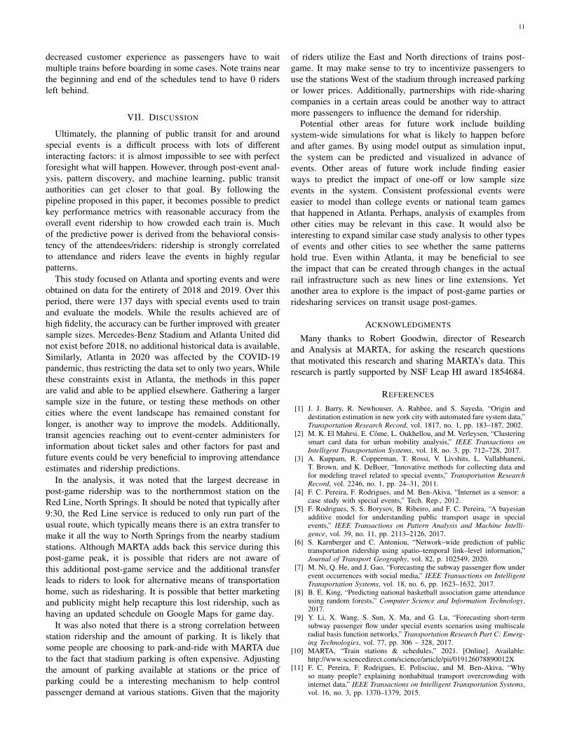
Figure 16 shows boxplots of the simulated wait times usingboth actual and proposed schedules. The number of trainsrepresented by the x markers. Note that, in most cases, themaximum wait time is decreased, as well as the 75th percentileand median.

Figure 17 highlights the percentage of people left be-hind by individual trains. The proposed schedules performed

Fig. 16: For each of the eight Atlanta United games with the upperdeck open, the two box plots compare simulated actual train schedulesvs. simulated proposed train schedules. Note the number of trains isrepresented with x markers.

Fig. 17: For each of the eight Atlanta United games with the upperdeck open, the percentage of ridership left behind for each trainis plotted for both simulations. The results from the simulations ofactual (recovered) schedules are in red and results from simulationswith proposed schedules are in blue. Note trains near the beginningand end of the schedules tend to have 0 riders left behind.

s

significantly better in this category as the demand matchesthe proposed train schedule more accurately. In the existingschedule, less than half the people at the station are able toboard the train. This could lead to potential crowding and

11

decreased customer experience as passengers have to waitmultiple trains before boarding in some cases. Note trains nearthe beginning and end of the schedules tend to have 0 ridersleft behind.

VII. DISCUSSION

Ultimately, the planning of public transit for and aroundspecial events is a difficult process with lots of differentinteracting factors: it is almost impossible to see with perfectforesight what will happen. However, through post-event anal-ysis, pattern discovery, and machine learning, public transitauthorities can get closer to that goal. By following thepipeline proposed in this paper, it becomes possible to predictkey performance metrics with reasonable accuracy from theoverall event ridership to how crowded each train is. Muchof the predictive power is derived from the behavioral consis-tency of the attendees/riders: ridership is strongly correlatedto attendance and riders leave the events in highly regularpatterns.

This study focused on Atlanta and sporting events and wereobtained on data for the entirety of 2018 and 2019. Over thisperiod, there were 137 days with special events used to trainand evaluate the models. While the results achieved are ofhigh fidelity, the accuracy can be further improved with greatersample sizes. Mercedes-Benz Stadium and Atlanta United didnot exist before 2018, no additional historical data is available,Similarly, Atlanta in 2020 was affected by the COVID-19pandemic, thus restricting the data set to only two years, Whilethese constraints exist in Atlanta, the methods in this paperare valid and able to be applied elsewhere. Gathering a largersample size in the future, or testing these methods on othercities where the event landscape has remained constant forlonger, is another way to improve the models. Additionally,transit agencies reaching out to event-center administers forinformation about ticket sales and other factors for past andfuture events could be very beneficial to improving attendanceestimates and ridership predictions.

In the analysis, it was noted that the largest decrease inpost-game ridership was to the northernmost station on theRed Line, North Springs. It should be noted that typically after9:30, the Red Line service is reduced to only run part of theusual route, which typically means there is an extra transfer tomake it all the way to North Springs from the nearby stadiumstations. Although MARTA adds back this service during thispost-game peak, it is possible that riders are not aware ofthis additional post-game service and the additional transferleads to riders to look for alternative means of transportationhome, such as ridesharing. It is possible that better marketingand publicity might help recapture this lost ridership, such ashaving an updated schedule on Google Maps for game day.

It was also noted that there is a strong correlation betweenstation ridership and the amount of parking. It is likely thatsome people are choosing to park-and-ride with MARTA dueto the fact that stadium parking is often expensive. Adjustingthe amount of parking available at stations or the price ofparking could be a interesting mechanism to help controlpassenger demand at various stations. Given that the majority

of riders utilize the East and North directions of trains post-game. It may make sense to try to incentivize passengers touse the stations West of the stadium through increased parkingor lower prices. Additionally, partnerships with ride-sharingcompanies in a certain areas could be another way to attractmore passengers to influence the demand for ridership.

Potential other areas for future work include buildingsystem-wide simulations for what is likely to happen beforeand after games. By using model output as simulation input,the system can be predicted and visualized in advance ofevents. Other areas of future work include finding easierways to predict the impact of one-off or low sample sizeevents in the system. Consistent professional events wereeasier to model than college events or national team gamesthat happened in Atlanta. Perhaps, analysis of examples fromother cities may be relevant in this case. It would also beinteresting to expand similar case study analysis to other typesof events and other cities to see whether the same patternshold true. Even within Atlanta, it may be beneficial to seethe impact that can be created through changes in the actualrail infrastructure such as new lines or line extensions. Yetanother area to explore is the impact of post-game parties orridesharing services on transit usage post-games.

ACKNOWLEDGMENTS

Many thanks to Robert Goodwin, director of Researchand Analysis at MARTA, for asking the research questionsthat motivated this research and sharing MARTA’s data. Thisresearch is partly supported by NSF Leap HI award 1854684.

REFERENCES

[1] J. J. Barry, R. Newhouser, A. Rahbee, and S. Sayeda, “Origin anddestination estimation in new york city with automated fare system data,”Transportation Research Record, vol. 1817, no. 1, pp. 183–187, 2002.

[2] M. K. El Mahrsi, E. Come, L. Oukhellou, and M. Verleysen, “Clusteringsmart card data for urban mobility analysis,” IEEE Transactions onIntelligent Transportation Systems, vol. 18, no. 3, pp. 712–728, 2017.

[3] A. Kuppam, R. Copperman, T. Rossi, V. Livshits, L. Vallabhaneni,T. Brown, and K. DeBoer, “Innovative methods for collecting data andfor modeling travel related to special events,” Transportation ResearchRecord, vol. 2246, no. 1, pp. 24–31, 2011.

[4] F. C. Pereira, F. Rodrigues, and M. Ben-Akiva, “Internet as a sensor: acase study with special events,” Tech. Rep., 2012.

[5] F. Rodrigues, S. S. Borysov, B. Ribeiro, and F. C. Pereira, “A bayesianadditive model for understanding public transport usage in specialevents,” IEEE Transactions on Pattern Analysis and Machine Intelli-gence, vol. 39, no. 11, pp. 2113–2126, 2017.

[6] S. Karnberger and C. Antoniou, “Network–wide prediction of publictransportation ridership using spatio–temporal link–level information,”Journal of Transport Geography, vol. 82, p. 102549, 2020.

[7] M. Ni, Q. He, and J. Gao, “Forecasting the subway passenger flow underevent occurrences with social media,” IEEE Transactions on IntelligentTransportation Systems, vol. 18, no. 6, pp. 1623–1632, 2017.

[8] B. E. King, “Predicting national basketball association game attendanceusing random forests,” Computer Science and Information Technology,2017.

[9] Y. Li, X. Wang, S. Sun, X. Ma, and G. Lu, “Forecasting short-termsubway passenger flow under special events scenarios using multiscaleradial basis function networks,” Transportation Research Part C: Emerg-ing Technologies, vol. 77, pp. 306 – 328, 2017.

[10] MARTA, “Train stations & schedules,” 2021. [Online]. Available:http://www.sciencedirect.com/science/article/pii/019126078890012X

[11] F. C. Pereira, F. Rodrigues, E. Polisciuc, and M. Ben-Akiva, “Whyso many people? explaining nonhabitual transport overcrowding withinternet data,” IEEE Transactions on Intelligent Transportation Systems,vol. 16, no. 3, pp. 1370–1379, 2015.

12

[12] L. McInnes, J. Healy, and S. Astels, “hdbscan: Hierarchical densitybased clustering,” Journal of Open Source Software, vol. 2, no. 11, p.205, 2017.

[13] C. Malzer and M. Baum, “A hybrid approach to hierarchical density-based cluster selection,” 2020 IEEE International Conference on Multi-sensor Fusion and Integration for Intelligent Systems (MFI), Sep 2020.

13

APPENDIX ABASELINE SIGNATURES

(a) Baseline Signature for Entries at North Ave Rail Station (b) Baseline Signature for Exits at North Ave Rail Station

(c) Baseline Signature for Entries at Midtown Rail Station (d) Baseline Signature for Exits at Midtown Rail Station

(e) Baseline Signature for Entries at Vine City Rail Station (f) Baseline Signature for Exits at Vine City Rail Station

Fig. 18: Baseline (non-event days) signature graphs for three stations showing the weekday (red) and weekend (blue) signatures for entries(left) and exits (right). The shaded region represents the 10th-90th percentile range for each bin.