1 PSR/A Multiband Polarimetric Imaging During Wakasa Bay (WBAY03) Field Campaign - Data Delivery Report to NASA PIs - B. Stankov, A.J. Gasiewski (PI), M. Klein, V. Leuski, V. Irisov, and B. Weber NOAA Environmental Laboratory Division of Microwave Systems Development 325 Broadway R/ET1 Boulder, CO 80305-3328 (303) 497-7275 [email protected]

Welcome message from author
This document is posted to help you gain knowledge. Please leave a comment to let me know what you think about it! Share it to your friends and learn new things together.
Transcript

1
PSR/A Multiband Polarimetric Imaging During Wakasa Bay (WBAY03)
Field Campaign
- Data Delivery Report to NASA PIs -
B. Stankov, A.J. Gasiewski (PI), M. Klein, V. Leuski, V. Irisov, and B. Weber
NOAA Environmental Laboratory
Division of Microwave Systems Development 325 Broadway R/ET1
Boulder, CO 80305-3328 (303) 497-7275
2
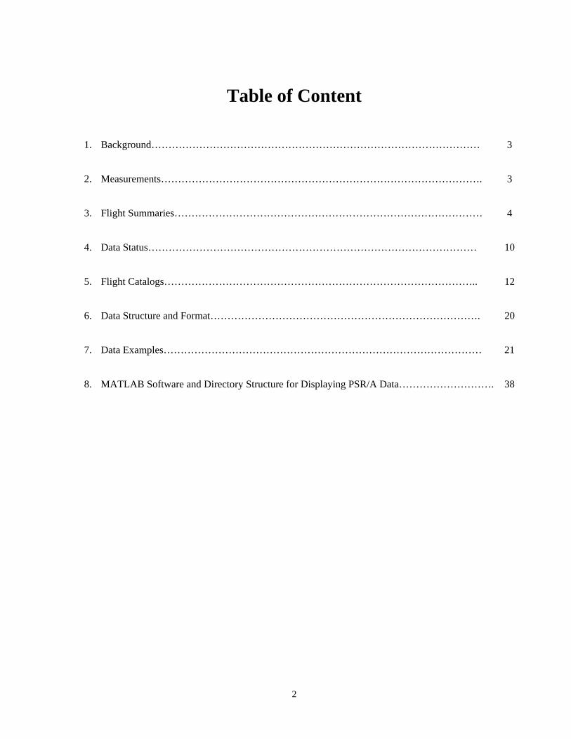
Table of Content
1. Background…………………………………………………………………………………… 3
2. Measurements…………………………………………………………………………………. 3
3. Flight Summaries……………………………………………………………………………… 4
4. Data Status…………………………………………………………………………………… 10
5. Flight Catalogs……………………………………………………………………………….. 12
6. Data Structure and Format……………………………………………………………………. 20
7. Data Examples………………………………………………………………………………… 21
8. MATLAB Software and Directory Structure for Displaying PSR/A Data………………………. 38

3
1. Background. In response to the need to estimate rainfall for both climate prediction and severe weather forecasting, ETL has developed a sensor for accurate calibration of existing and planned satellite microwave rainfall instruments. The sensor, based on the ETL Polarimetric Scanning Radiometer (PSR) system, is the first airborne conical-scanning radiometer system, and is able to image rainfall in regions inaccessible by the land-based rain radars, e.g. WSR-88D radar. The system was first flown for rainfall measurement in 1998 and provided images of the rainbands of Hurricane Bonnie at landfall on the North Carolina coastline. As the result of a joint U.S.-Japanese collaboration involving NOAA, NASA, and the Japanese Space Agency NASDA, the PSR is providing data for calibration of the NASA-NASDA AMSR-E sensor on the NASA Aqua satellite over the Sea of Japan and Pacific coastal region east of Japan. Currently, NOAA/NESDIS plans to use the AMSR-E data in operational algorithms and as a means of improving rainfall algorithms in preparation for the launch of NPOESS at the end of the decade. Data from high-resolution airborne instruments such as the PSR is critical for both on-orbit assessment of the performance of sensors such as AMSR-E, AMSU, and CMIS, as well as improving the accuracy of operational satellite rainfall algorithms. The resolution of the PSR is at least a factor of ten greater than that of satellites, and thus provides a means of resolving the structure of rain-producing frontal systems that are otherwise impossible to observe from space. Improved rainfall estimation is essential for quantitative precipitation forecasting (e.g., flash flood, hurricanes at landfall, other high-impact weather such as coastal storms), drought monitoring and prediction, and global climate change assessment. This document provides information for the WBAY03 team scientists about the first version of processed PSR/A data collected during the field campaign and delivered to the National Snow and Ice Data Center (NSIDC) for archiving as part of the WBAY03 combined dataset and to the Principal Investigator, Tom Wilheit in May 2004.
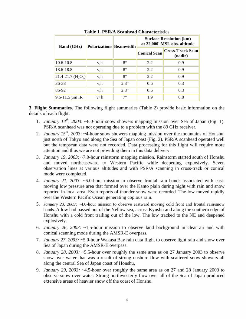
2. Measurements. The PSR configuration on the NASA P-3 N426NA aircraft during the 2003 Wakasa Bay experiment uses the NOAA PSR/A scanhead (Table. 1) operated in both conical and cross-track scanned mode. The conical mode uses an incidence angle of 55 degrees from nadir. The purposes of collecting this data are:
• To study the impact of melting level on passive microwave rain signatures collected coincidentally with multiband (Ku, Ka, and W) scanning Doppler rain/cloud radars. The joint data provides a unique basis for algorithm improvement for NASA TRMM and algorithm development for the future NASA Global Precipitation Mission (GPM).
• To provide high resolution multiband microwave radiometric imagery for: • AMSR-E calibration and rain rate/snow retrieval validation studies. • NOAA-NASA Joint Center for Satellite Data Assimilation (JCSDA) radiative transfer
modeling studies. • NPOESS CMIS and WindSat passive wind vector algorithm development.
PSR imaging occurred at medium altitude (~22,000' MSL) during flight lines crossing maritime and orographic precipitation. Cases of both snow and moderate to light rain were observed with melting levels from the surface up to ~8,000'. Several low-altitude (~700' MSL) lines were also flown for surface emission studies. Extensive thermal stabilization of PSR/A radiometers, refurbishment of the PSR/A 18/21 and 89 GHz receivers, and installation of new 37 GHz LNAs account for much improved stability.
4
Table 1. PSR/A Scanhead Characteristics Surface Resolution (km)
at 22,000' MSL obs. altitude Band (GHz) Polarizations Beamwidth Conical Scan Cross-Track Scan
(nadir) 10.6-10.8 v,h 8° 2.2 0.9 18.6-18.8 v,h 8° 2.2 0.9 21.4-21.7 (H2Ov) v,h 8° 2.2 0.9 36-38 v,h 2.3° 0.6 0.3 86-92 v,h 2.3° 0.6 0.3 9.6-11.5 µm IR v+h 7° 1.9 0.8
3. Flight Summaries. The following flight summaries (Table 2) provide basic information on the details of each flight.
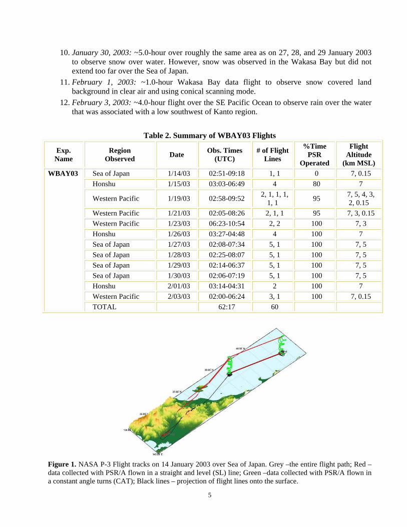
1. January 14th, 2003: ~6.0-hour snow showers mapping mission over Sea of Japan (Fig. 1). PSR/A scanhead was not operating due to a problem with the 89 GHz receiver.
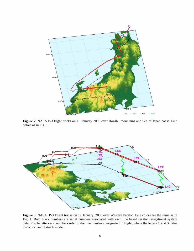
2. January 15th, 2003: ~4-hour snow showers mapping mission over the mountains of Honshu, just north of Tokyo and along the Sea of Japan coast (Fig. 2). PSR/A scanhead operated well but the tempscan data were not recorded. Data processing for this flight will require more attention and thus we are not providing them in this data delivery.
3. January 19, 2003: ~7.0-hour rainstorm mapping mission. Rainstorm started south of Honshu and moved northeastward to Western Pacific while deepening explosively. Seven observation lines at various altitudes and with PSR/A scanning in cross-track or conical mode were completed.
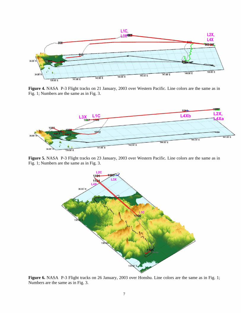
4. January 21, 2003: ~6.0-hour mission to observe frontal rain bands associated with east-moving low pressure area that formed over the Kanto plain during night with rain and snow reported in local area. Even reports of thunder-snow were recorded. The low moved rapidly over the Western Pacific Ocean generating copious rain.
5. January 23, 2003: ~4.0-hour mission to observe eastward moving cold front and frontal rain/snow bands. A low had passed out of the Yellow sea, across Kyushu and along the southern edge of Honshu with a cold front trailing out of the low. The low tracked to the NE and deepened explosively.
6. January 26, 2003: ~1.5-hour mission to observe land background in clear air and with conical scanning mode during the AMSR-E overpass.
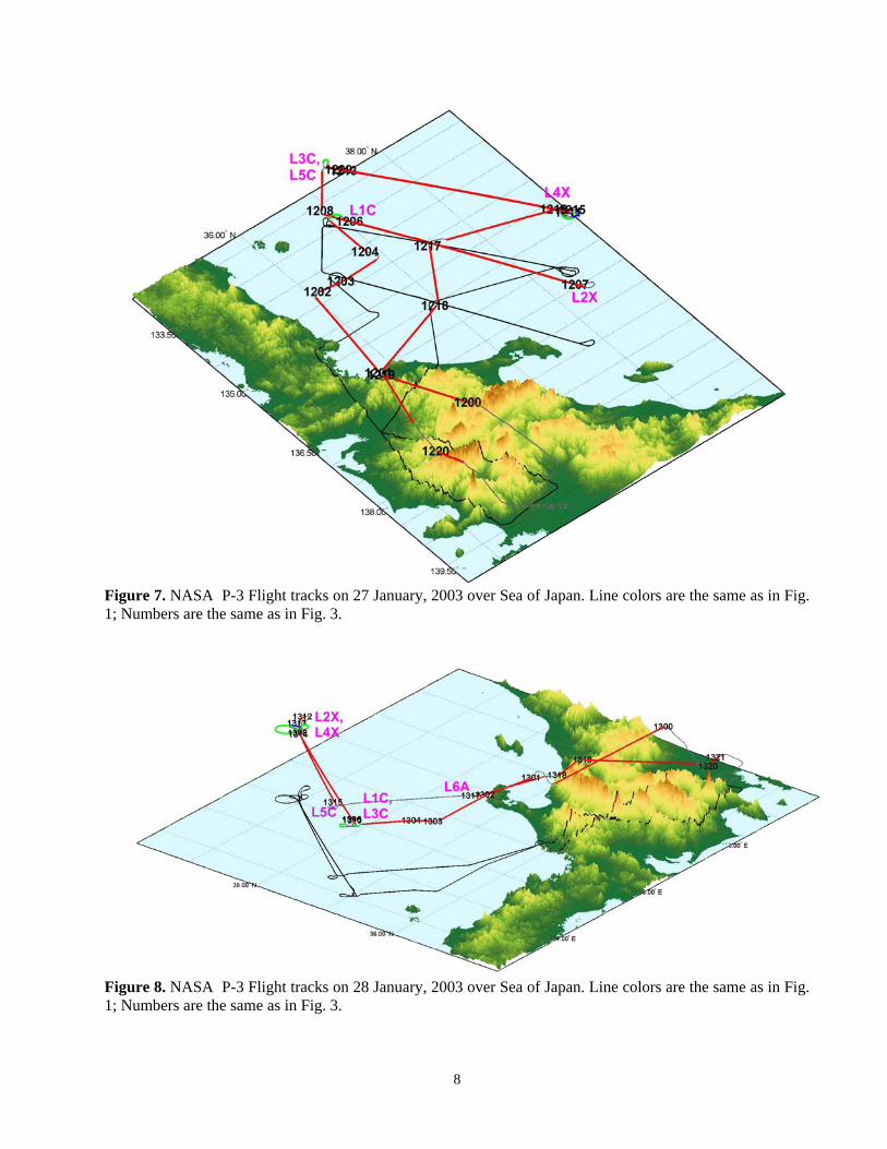
7. January 27, 2003: ~5.0-hour Wakasa Bay rain data flight to observe light rain and snow over Sea of Japan during the AMSR-E overpass.
8. January 28, 2003: ~5.5-hour over roughly the same area as on 27 January 2003 to observe snow over water that was a result of strong onshore flow with scattered snow showers all along the central Sea of Japan coast of Honshu.
9. January 29, 2003: ~4.5-hour over roughly the same area as on 27 and 28 January 2003 to observe snow over water. Strong northwesterly flow over all of the Sea of Japan produced extensive areas of heavier snow off the coast of Honshu.
5
10. January 30, 2003: ~5.0-hour over roughly the same area as on 27, 28, and 29 January 2003 to observe snow over water. However, snow was observed in the Wakasa Bay but did not extend too far over the Sea of Japan.
11. February 1, 2003: ~1.0-hour Wakasa Bay data flight to observe snow covered land background in clear air and using conical scanning mode.
12. February 3, 2003: ~4.0-hour flight over the SE Pacific Ocean to observe rain over the water that was associated with a low southwest of Kanto region.
Table 2. Summary of WBAY03 Flights
Exp. Name
Region Observed Date Obs. Times
(UTC) # of Flight
Lines
%Time PSR
Operated
Flight Altitude
(km MSL) Sea of Japan 1/14/03 02:51-09:18 1, 1 0 7, 0.15 Honshu 1/15/03 03:03-06:49 4 80 7
Western Pacific 1/19/03 02:58-09:52 2, 1, 1, 1, 1, 1 95 7, 5, 4, 3,
2, 0.15 Western Pacific 1/21/03 02:05-08:26 2, 1, 1 95 7, 3, 0.15 Western Pacific 1/23/03 06:23-10:54 2, 2 100 7, 3 Honshu 1/26/03 03:27-04:48 4 100 7 Sea of Japan 1/27/03 02:08-07:34 5, 1 100 7, 5 Sea of Japan 1/28/03 02:25-08:07 5, 1 100 7, 5 Sea of Japan 1/29/03 02:14-06:37 5, 1 100 7, 5 Sea of Japan 1/30/03 02:06-07:19 5, 1 100 7, 5 Honshu 2/01/03 03:14-04:31 2 100 7 Western Pacific 2/03/03 02:00-06:24 3, 1 100 7, 0.15
WBAY03
TOTAL 62:17 60
Figure 1. NASA P-3 Flight tracks on 14 January 2003 over Sea of Japan. Grey –the entire flight path; Red –data collected with PSR/A flown in a straight and level (SL) line; Green –data collected with PSR/A flown in a constant angle turns (CAT); Black lines – projection of flight lines onto the surface.
6
Figure 2. NASA P-3 flight tracks on 15 January 2003 over Honshu mountains and Sea of Japan coast. Line colors as in Fig. 1.
Figure 3. NASA P-3 Flight tracks on 19 January, 2003 over Western Pacific. Line colors are the same as in Fig. 1; Bold black numbers are serial numbers associated with each line based on the navigational system data; Purple letters and numbers refer to the line numbers designated in flight, where the letters C and X refer to conical and X-track mode.
7
Figure 4. NASA P-3 Flight tracks on 21 January, 2003 over Western Pacific. Line colors are the same as in Fig. 1; Numbers are the same as in Fig. 3.
Figure 5. NASA P-3 Flight tracks on 23 January, 2003 over Western Pacific. Line colors are the same as in Fig. 1; Numbers are the same as in Fig. 3.
Figure 6. NASA P-3 Flight tracks on 26 January, 2003 over Honshu. Line colors are the same as in Fig. 1; Numbers are the same as in Fig. 3.
8
Figure 7. NASA P-3 Flight tracks on 27 January, 2003 over Sea of Japan. Line colors are the same as in Fig. 1; Numbers are the same as in Fig. 3.
Figure 8. NASA P-3 Flight tracks on 28 January, 2003 over Sea of Japan. Line colors are the same as in Fig. 1; Numbers are the same as in Fig. 3.
9
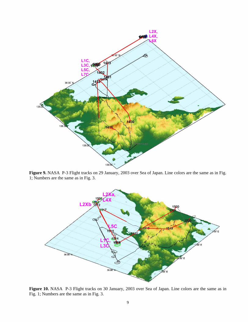
Figure 9. NASA P-3 Flight tracks on 29 January, 2003 over Sea of Japan. Line colors are the same as in Fig. 1; Numbers are the same as in Fig. 3.
Figure 10. NASA P-3 Flight tracks on 30 January, 2003 over Sea of Japan. Line colors are the same as in Fig. 1; Numbers are the same as in Fig. 3.
10
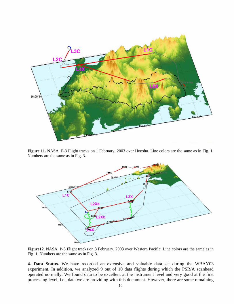
Figure 11. NASA P-3 Flight tracks on 1 February, 2003 over Honshu. Line colors are the same as in Fig. 1; Numbers are the same as in Fig. 3.
Figure12. NASA P-3 Flight tracks on 3 February, 2003 over Western Pacific. Line colors are the same as in Fig. 1; Numbers are the same as in Fig. 3. 4. Data Status. We have recorded an extensive and valuable data set during the WBAY03 experiment. In addition, we analyzed 9 out of 10 data flights during which the PSR/A scanhead operated normally. We found data to be excellent at the instrument level and very good at the first processing level, i.e., data we are providing with this document. However, there are some remaining
11
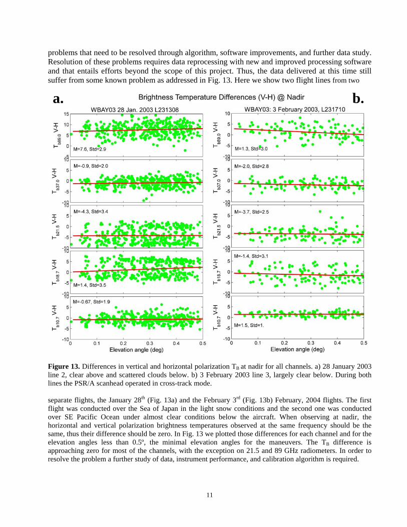
problems that need to be resolved through algorithm, software improvements, and further data study. Resolution of these problems requires data reprocessing with new and improved processing software and that entails efforts beyond the scope of this project. Thus, the data delivered at this time still suffer from some known problem as addressed in Fig. 13. Here we show two flight lines from two
Figure 13. Differences in vertical and horizontal polarization TB at nadir for all channels. a) 28 January 2003 line 2, clear above and scattered clouds below. b) 3 February 2003 line 3, largely clear below. During both lines the PSR/A scanhead operated in cross-track mode. separate flights, the January 28th (Fig. 13a) and the February 3rd (Fig. 13b) February, 2004 flights. The first flight was conducted over the Sea of Japan in the light snow conditions and the second one was conducted over SE Pacific Ocean under almost clear conditions below the aircraft. When observing at nadir, the horizontal and vertical polarization brightness temperatures observed at the same frequency should be the same, thus their difference should be zero. In Fig. 13 we plotted those differences for each channel and for the elevation angles less than 0.5º, the minimal elevation angles for the maneuvers. The TB difference is approaching zero for most of the channels, with the exception on 21.5 and 89 GHz radiometers. In order to resolve the problem a further study of data, instrument performance, and calibration algorithm is required.
a. b.
12
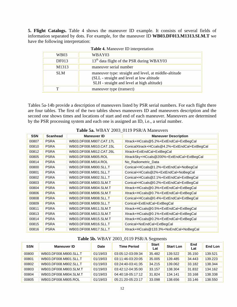
5. Flight Catalogs. Table 4 shows the maneuver ID example. It consists of several fields of information separated by dots. For example, for the maneuver ID WB03.DF013.M1313.SLM.T we have the following interpretation:
Table 4. Maneuver ID interpretation WB03 WBAY03 DF013 13th data flight of the PSR during WBAY03 M1313 maneuver serial number SLM maneuver type: straight and level, at middle-altitude
(SLL - straight and level at low altitude SLH - straight and level at high altitude)
T maneuver type (transect)
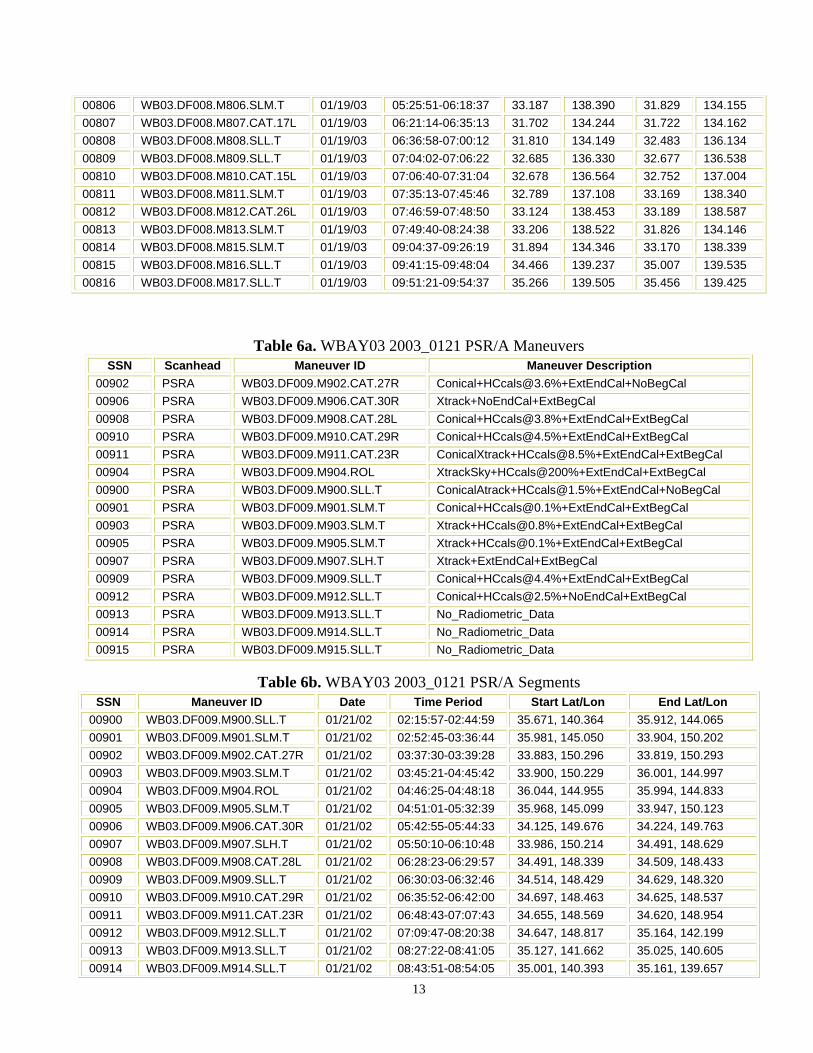
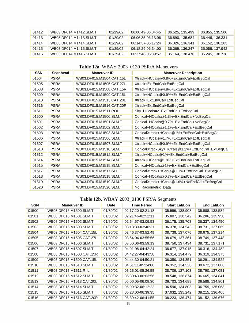
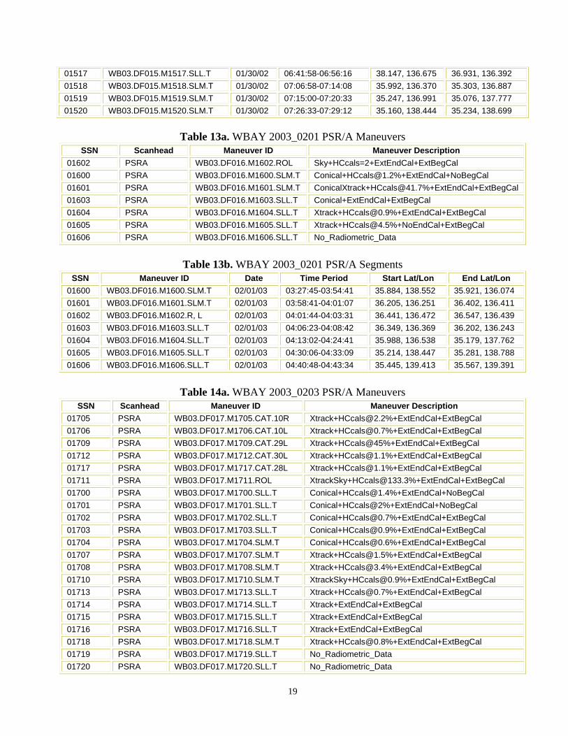
Tables 5a-14b provide a description of maneuvers listed by PSR serial numbers. For each flight there are four tables. The first of the two tables shows maneuvers ID and maneuvers description and the second one shows times and locations of start and end of each maneuver. Maneuvers are determined by the PSR processing system and each one is assigned an ID, i.e., a serial number.
Table 5a. WBAY 2003_0119 PSR/A Maneuvers SSN Scanhead Maneuver ID Maneuver Description
00807 PSRA WB03.DF008.M807.CAT.17L [email protected]%+ExtEndCal+ExtBegCal 00810 PSRA WB03.DF008.M810.CAT.15L [email protected]%+ExtEndCal+ExtBegCal 00812 PSRA WB03.DF008.M812.CAT.26L Xtrack+ExtEndCal+ExtBegCal 00805 PSRA WB03.DF008.M805.ROL XtrackSky+HCcals@200%+ExtEndCal+ExtBegCal 00814 PSRA WB03.DF008.M814.ROL No_Radiometric_Data 00800 PSRA WB03.DF008.M800.SLL.T [email protected]%+ExtEndCal+NoBegCal 00801 PSRA WB03.DF008.M801.SLL.T Conical+HCcals@2%+ExtEndCal+NoBegCal 00802 PSRA WB03.DF008.M802.SLL.T [email protected]%+ExtEndCal+ExtBegCal 00803 PSRA WB03.DF008.M803.SLM.T [email protected]%+ExtEndCal+ExtBegCal 00804 PSRA WB03.DF008.M804.SLM.T [email protected]%+ExtEndCal+ExtBegCal 00806 PSRA WB03.DF008.M806.SLM.T [email protected]%+ExtEndCal+ExtBegCal 00808 PSRA WB03.DF008.M808.SLL.T [email protected]%+ExtEndCal+ExtBegCal 00809 PSRA WB03.DF008.M809.SLL.T Conical+ExtEndCal+ExtBegCal 00811 PSRA WB03.DF008.M811.SLM.T [email protected]%+ExtEndCal+ExtBegCal 00813 PSRA WB03.DF008.M813.SLM.T [email protected]%+ExtEndCal+ExtBegCal 00814 PSRA WB03.DF008.M815.SLM.T [email protected]%+ExtEndCal+ExtBegCal� 00815 PSRA WB03.DF008.M816.SLL.T Conical+NoEndCal+ExtBegCal 00816 PSRA WB03.DF008.M817.SLL.T [email protected]%+NoEndCal+NoBegCal
Table 5b. WBAY 2003_0119 PSR/A Segments
SSN Maneuver ID Date Time Period Start Lat Start Lon End
Lat End Lon
00800 WB03.DF008.M800.SLL.T 01/19/03 03:05:12-03:09:34 35.482 139.522 35.150 139.521 00801 WB03.DF008.M801.SLL.T 01/19/03 03:11:46-03:20:05 35.005 139.485 34.443 139.223 00802 WB03.DF008.M802.SLL.T 01/19/03 03:24:40-03:41:35 34.215 139.062 33.182 138.344 00803 WB03.DF008.M803.SLM.T 01/19/03 03:42:12-04:35:00 33.157 138.304 31.832 134.162 00804 WB03.DF008.M804.SLM.T 01/19/03 04:40:18-05:17:12 31.824 134.141 33.168 138.338 00805 WB03.DF008.M805.ROL 01/19/03 05:21:20-05:23:17 33.098 138.656 33.146 138.550
13
00806 WB03.DF008.M806.SLM.T 01/19/03 05:25:51-06:18:37 33.187 138.390 31.829 134.155 00807 WB03.DF008.M807.CAT.17L 01/19/03 06:21:14-06:35:13 31.702 134.244 31.722 134.162 00808 WB03.DF008.M808.SLL.T 01/19/03 06:36:58-07:00:12 31.810 134.149 32.483 136.134 00809 WB03.DF008.M809.SLL.T 01/19/03 07:04:02-07:06:22 32.685 136.330 32.677 136.538 00810 WB03.DF008.M810.CAT.15L 01/19/03 07:06:40-07:31:04 32.678 136.564 32.752 137.004 00811 WB03.DF008.M811.SLM.T 01/19/03 07:35:13-07:45:46 32.789 137.108 33.169 138.340 00812 WB03.DF008.M812.CAT.26L 01/19/03 07:46:59-07:48:50 33.124 138.453 33.189 138.587 00813 WB03.DF008.M813.SLM.T 01/19/03 07:49:40-08:24:38 33.206 138.522 31.826 134.146 00814 WB03.DF008.M815.SLM.T 01/19/03 09:04:37-09:26:19 31.894 134.346 33.170 138.339 00815 WB03.DF008.M816.SLL.T 01/19/03 09:41:15-09:48:04 34.466 139.237 35.007 139.535 00816 WB03.DF008.M817.SLL.T 01/19/03 09:51:21-09:54:37 35.266 139.505 35.456 139.425
Table 6a. WBAY03 2003_0121 PSR/A Maneuvers
SSN Scanhead Maneuver ID Maneuver Description 00902 PSRA WB03.DF009.M902.CAT.27R [email protected]%+ExtEndCal+NoBegCal 00906 PSRA WB03.DF009.M906.CAT.30R Xtrack+NoEndCal+ExtBegCal 00908 PSRA WB03.DF009.M908.CAT.28L [email protected]%+ExtEndCal+ExtBegCal 00910 PSRA WB03.DF009.M910.CAT.29R [email protected]%+ExtEndCal+ExtBegCal 00911 PSRA WB03.DF009.M911.CAT.23R [email protected]%+ExtEndCal+ExtBegCal 00904 PSRA WB03.DF009.M904.ROL XtrackSky+HCcals@200%+ExtEndCal+ExtBegCal 00900 PSRA WB03.DF009.M900.SLL.T [email protected]%+ExtEndCal+NoBegCal 00901 PSRA WB03.DF009.M901.SLM.T [email protected]%+ExtEndCal+ExtBegCal 00903 PSRA WB03.DF009.M903.SLM.T [email protected]%+ExtEndCal+ExtBegCal 00905 PSRA WB03.DF009.M905.SLM.T [email protected]%+ExtEndCal+ExtBegCal 00907 PSRA WB03.DF009.M907.SLH.T Xtrack+ExtEndCal+ExtBegCal 00909 PSRA WB03.DF009.M909.SLL.T [email protected]%+ExtEndCal+ExtBegCal 00912 PSRA WB03.DF009.M912.SLL.T [email protected]%+NoEndCal+ExtBegCal 00913 PSRA WB03.DF009.M913.SLL.T No_Radiometric_Data 00914 PSRA WB03.DF009.M914.SLL.T No_Radiometric_Data 00915 PSRA WB03.DF009.M915.SLL.T No_Radiometric_Data
Table 6b. WBAY03 2003_0121 PSR/A Segments SSN Maneuver ID Date Time Period Start Lat/Lon End Lat/Lon
00900 WB03.DF009.M900.SLL.T 01/21/02 02:15:57-02:44:59 35.671, 140.364 35.912, 144.065 00901 WB03.DF009.M901.SLM.T 01/21/02 02:52:45-03:36:44 35.981, 145.050 33.904, 150.202 00902 WB03.DF009.M902.CAT.27R 01/21/02 03:37:30-03:39:28 33.883, 150.296 33.819, 150.293 00903 WB03.DF009.M903.SLM.T 01/21/02 03:45:21-04:45:42 33.900, 150.229 36.001, 144.997 00904 WB03.DF009.M904.ROL 01/21/02 04:46:25-04:48:18 36.044, 144.955 35.994, 144.833 00905 WB03.DF009.M905.SLM.T 01/21/02 04:51:01-05:32:39 35.968, 145.099 33.947, 150.123 00906 WB03.DF009.M906.CAT.30R 01/21/02 05:42:55-05:44:33 34.125, 149.676 34.224, 149.763 00907 WB03.DF009.M907.SLH.T 01/21/02 05:50:10-06:10:48 33.986, 150.214 34.491, 148.629 00908 WB03.DF009.M908.CAT.28L 01/21/02 06:28:23-06:29:57 34.491, 148.339 34.509, 148.433 00909 WB03.DF009.M909.SLL.T 01/21/02 06:30:03-06:32:46 34.514, 148.429 34.629, 148.320 00910 WB03.DF009.M910.CAT.29R 01/21/02 06:35:52-06:42:00 34.697, 148.463 34.625, 148.537 00911 WB03.DF009.M911.CAT.23R 01/21/02 06:48:43-07:07:43 34.655, 148.569 34.620, 148.954 00912 WB03.DF009.M912.SLL.T 01/21/02 07:09:47-08:20:38 34.647, 148.817 35.164, 142.199 00913 WB03.DF009.M913.SLL.T 01/21/02 08:27:22-08:41:05 35.127, 141.662 35.025, 140.605 00914 WB03.DF009.M914.SLL.T 01/21/02 08:43:51-08:54:05 35.001, 140.393 35.161, 139.657
14
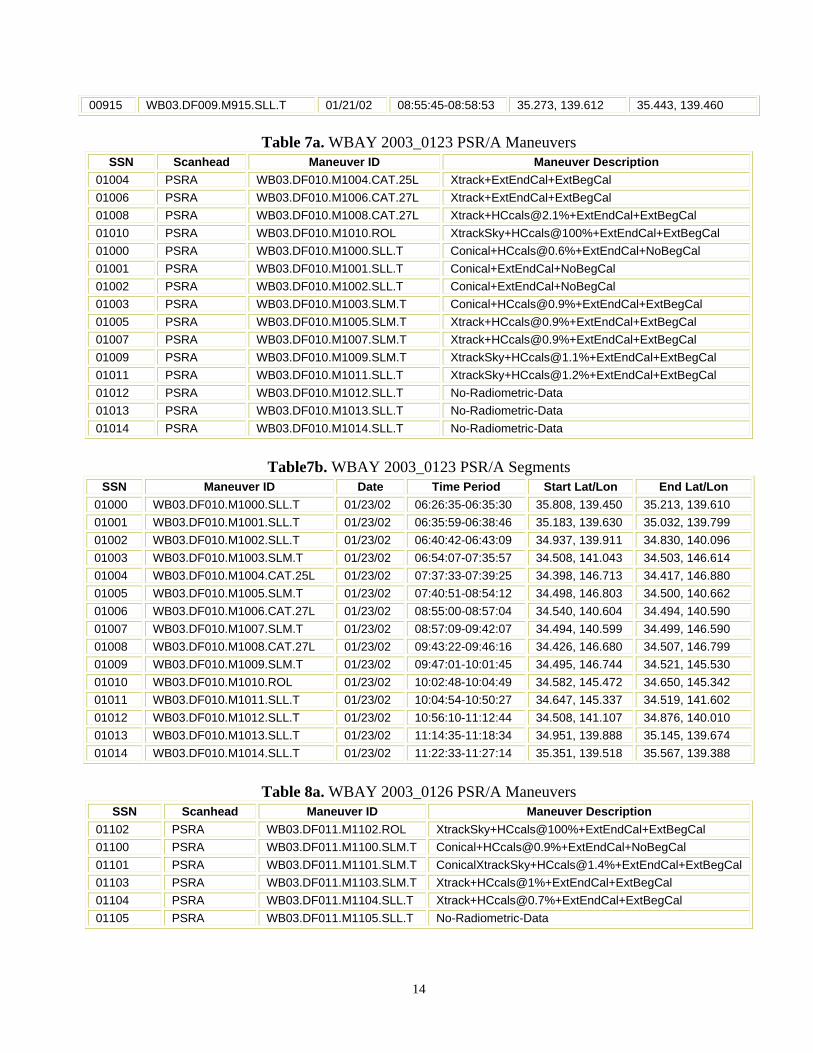
00915 WB03.DF009.M915.SLL.T 01/21/02 08:55:45-08:58:53 35.273, 139.612 35.443, 139.460
Table 7a. WBAY 2003_0123 PSR/A Maneuvers
SSN Scanhead Maneuver ID Maneuver Description 01004 PSRA WB03.DF010.M1004.CAT.25L Xtrack+ExtEndCal+ExtBegCal 01006 PSRA WB03.DF010.M1006.CAT.27L Xtrack+ExtEndCal+ExtBegCal 01008 PSRA WB03.DF010.M1008.CAT.27L [email protected]%+ExtEndCal+ExtBegCal 01010 PSRA WB03.DF010.M1010.ROL XtrackSky+HCcals@100%+ExtEndCal+ExtBegCal 01000 PSRA WB03.DF010.M1000.SLL.T [email protected]%+ExtEndCal+NoBegCal 01001 PSRA WB03.DF010.M1001.SLL.T Conical+ExtEndCal+NoBegCal 01002 PSRA WB03.DF010.M1002.SLL.T Conical+ExtEndCal+NoBegCal 01003 PSRA WB03.DF010.M1003.SLM.T [email protected]%+ExtEndCal+ExtBegCal 01005 PSRA WB03.DF010.M1005.SLM.T [email protected]%+ExtEndCal+ExtBegCal 01007 PSRA WB03.DF010.M1007.SLM.T [email protected]%+ExtEndCal+ExtBegCal 01009 PSRA WB03.DF010.M1009.SLM.T [email protected]%+ExtEndCal+ExtBegCal 01011 PSRA WB03.DF010.M1011.SLL.T [email protected]%+ExtEndCal+ExtBegCal 01012 PSRA WB03.DF010.M1012.SLL.T No-Radiometric-Data 01013 PSRA WB03.DF010.M1013.SLL.T No-Radiometric-Data 01014 PSRA WB03.DF010.M1014.SLL.T No-Radiometric-Data
Table7b. WBAY 2003_0123 PSR/A Segments
SSN Maneuver ID Date Time Period Start Lat/Lon End Lat/Lon 01000 WB03.DF010.M1000.SLL.T 01/23/02 06:26:35-06:35:30 35.808, 139.450 35.213, 139.610 01001 WB03.DF010.M1001.SLL.T 01/23/02 06:35:59-06:38:46 35.183, 139.630 35.032, 139.799 01002 WB03.DF010.M1002.SLL.T 01/23/02 06:40:42-06:43:09 34.937, 139.911 34.830, 140.096 01003 WB03.DF010.M1003.SLM.T 01/23/02 06:54:07-07:35:57 34.508, 141.043 34.503, 146.614 01004 WB03.DF010.M1004.CAT.25L 01/23/02 07:37:33-07:39:25 34.398, 146.713 34.417, 146.880 01005 WB03.DF010.M1005.SLM.T 01/23/02 07:40:51-08:54:12 34.498, 146.803 34.500, 140.662 01006 WB03.DF010.M1006.CAT.27L 01/23/02 08:55:00-08:57:04 34.540, 140.604 34.494, 140.590 01007 WB03.DF010.M1007.SLM.T 01/23/02 08:57:09-09:42:07 34.494, 140.599 34.499, 146.590 01008 WB03.DF010.M1008.CAT.27L 01/23/02 09:43:22-09:46:16 34.426, 146.680 34.507, 146.799 01009 WB03.DF010.M1009.SLM.T 01/23/02 09:47:01-10:01:45 34.495, 146.744 34.521, 145.530 01010 WB03.DF010.M1010.ROL 01/23/02 10:02:48-10:04:49 34.582, 145.472 34.650, 145.342 01011 WB03.DF010.M1011.SLL.T 01/23/02 10:04:54-10:50:27 34.647, 145.337 34.519, 141.602 01012 WB03.DF010.M1012.SLL.T 01/23/02 10:56:10-11:12:44 34.508, 141.107 34.876, 140.010 01013 WB03.DF010.M1013.SLL.T 01/23/02 11:14:35-11:18:34 34.951, 139.888 35.145, 139.674 01014 WB03.DF010.M1014.SLL.T 01/23/02 11:22:33-11:27:14 35.351, 139.518 35.567, 139.388
Table 8a. WBAY 2003_0126 PSR/A Maneuvers
SSN Scanhead Maneuver ID Maneuver Description 01102 PSRA WB03.DF011.M1102.ROL XtrackSky+HCcals@100%+ExtEndCal+ExtBegCal 01100 PSRA WB03.DF011.M1100.SLM.T [email protected]%+ExtEndCal+NoBegCal 01101 PSRA WB03.DF011.M1101.SLM.T [email protected]%+ExtEndCal+ExtBegCal 01103 PSRA WB03.DF011.M1103.SLM.T Xtrack+HCcals@1%+ExtEndCal+ExtBegCal 01104 PSRA WB03.DF011.M1104.SLL.T [email protected]%+ExtEndCal+ExtBegCal 01105 PSRA WB03.DF011.M1105.SLL.T No-Radiometric-Data
15
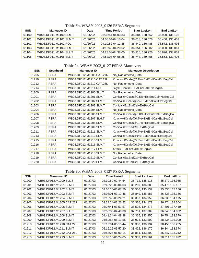
Table 8b. WBAY 2003_0126 PSR/A Segments SSN Maneuver ID Date Time Period Start Lat/Lon End Lat/Lon
01100 WB03.DF011.M1100.SLM.T 01/26/02 03:38:54-04:03:33 35.884, 138.552 35.920, 136.105 01101 WB03.DF011.M1101.SLM.T 01/26/02 04:05:04-04:10:04 36.018, 136.076 36.400, 136.409 01102 WB03.DF011.M1102.ROL 01/26/02 04:10:52-04:12:35 36.440, 136.488 36.572, 136.493 01103 WB03.DF011.M1103.SLM.T 01/26/02 04:15:40-04:20:52 36.354, 136.382 36.000, 136.061 01104 WB03.DF011.M1104.SLL.T 01/26/02 04:23:08-04:38:05 35.916, 136.226 35.896, 138.039 01105 WB03.DF011.M1105.SLL.T 01/26/02 04:52:08-04:56:28 35.747, 139.455 35.563, 139.403
Table 9a. WBAY 2003_0127 PSR/A Maneuvers
SSN Scanhead Maneuver ID Maneuver Description 01205 PSRA WB03.DF012.M1205.CAT.27R No_Radiometric_Data 01210 PSRA WB03.DF012.M1210.CAT.27L [email protected]%+ExtEndCal+ExtBegCal 01212 PSRA WB03.DF012.M1212.CAT.26L No_Radiometric_Data 01214 PSRA WB03.DF012.M1214.ROL Sky+HCcals=2+ExtEndCal+ExtBegCal 01200 PSRA WB03.DF012.M1200.SLL.T No_Radiometric_Data 01201 PSRA WB03.DF012.M1201.SLM.T [email protected]%+ExtEndCal+NoBegCal 01202 PSRA WB03.DF012.M1202.SLM.T Conical+HCcals@2%+ExtEndCal+ExtBegCal 01203 PSRA WB03.DF012.M1203.SLM.T Conical+ExtEndCal+ExtBegCal 01204 PSRA WB03.DF012.M1204.SLM.T No_Radiometric_Data 01206 PSRA WB03.DF012.M1206.SLM.T [email protected]%+ExtEndCal+ExtBegCal 01207 PSRA WB03.DF012.M1207.SLH.T [email protected]%+ExtEndCal+ExtBegCal 01208 PSRA WB03.DF012.M1208.SLM.T [email protected]%+ExtEndCal+ExtBegCal 01209 PSRA WB03.DF012.M1209.SLM.T Conical+ExtEndCal+ExtBegCal 01211 PSRA WB03.DF012.M1211.SLM.T [email protected]%+ExtEndCal+ExtBegCal 01213 PSRA WB03.DF012.M1213.SLM.T Conical+HCcals@1%+ExtEndCal+ExtBegCal 01215 PSRA WB03.DF012.M1215.SLM.T [email protected]%+ExtEndCal+ExtBegCal 01216 PSRA WB03.DF012.M1216.SLM.T [email protected]%+ExtEndCal+ExtBegCal 01217 PSRA WB03.DF012.M1217.SLM.T Xtrack+ExtEndCal+ExtBegCal 01218 PSRA WB03.DF012.M1218.SLM.T No_Radiometric_Data 01219 PSRA WB03.DF012.M1219.SLM.T Conical+ExtEndCal+ExtBegCal 01220 PSRA WB03.DF012.M1220.SLM.T Conical+ExtEndCal+ExtBegCal
Table 9b. WBAY 2003_0127 PSR/A Segments
SSN Maneuver ID Date Time Period Start Lat/Lon End Lat/Lon 01200 WB03.DF012.M1200.SLL.T 01/27/03 02:30:50-02:44:54 35.712, 138.116 35.272,136.935 01201 WB03.DF012.M1201.SLM.T 01/27/03 02:45:28-03:04:03 35.269, 136.883 35.475,135.187 01202 WB03.DF012.M1202.SLM.T 01/27/03 03:05:10-03:07:50 35.556, 135.137 35.830,135.186 01203 WB03.DF012.M1203.SLM.T 01/27/03 03:08:01-03:12:46 35.849, 135.187 36.338,135.166 01204 WB03.DF012.M1204.SLM.T 01/27/03 03:15:48-03:24:21 36.337, 134.959 36.336,134.175 01205 WB03.DF012.M1205.CAT.27R 01/27/03 03:24:24-03:26:22 36.336, 134.171 36.474,134.204 01206 WB03.DF012.M1206.SLM.T 01/27/03 03:27:41-03:51:57 36.503, 134.373 37.801,137.419 01207 WB03.DF012.M1207.SLH.T 01/27/03 03:56:35-04:40:38 37.761, 137.309 36.348,134.032 01208 WB03.DF012.M1208.SLM.T 01/27/03 04:41:34-04:48:38 36.365, 133.950 36.754,133.370 01209 WB03.DF012.M1209.SLM.T 01/27/03 04:50:54-05:11:55 36.924, 133.502 38.334,136.000 01210 WB03.DF012.M1210.CAT.27L 01/27/03 05:13:01-05:15:44 38.330, 136.134 38.453,136.205 01211 WB03.DF012.M1211.SLM.T 01/27/03 05:16:25-05:57:20 38.422, 136.170 36.844,133.374 01212 WB03.DF012.M1212.CAT.26L 01/27/03 05:58:26-06:00:14 36.881, 133.300 36.847,133.242 01213 WB03.DF012.M1213.SLM.T 01/27/03 06:03:15-06:24:05 36.953, 133.561 38.311,135.972
16
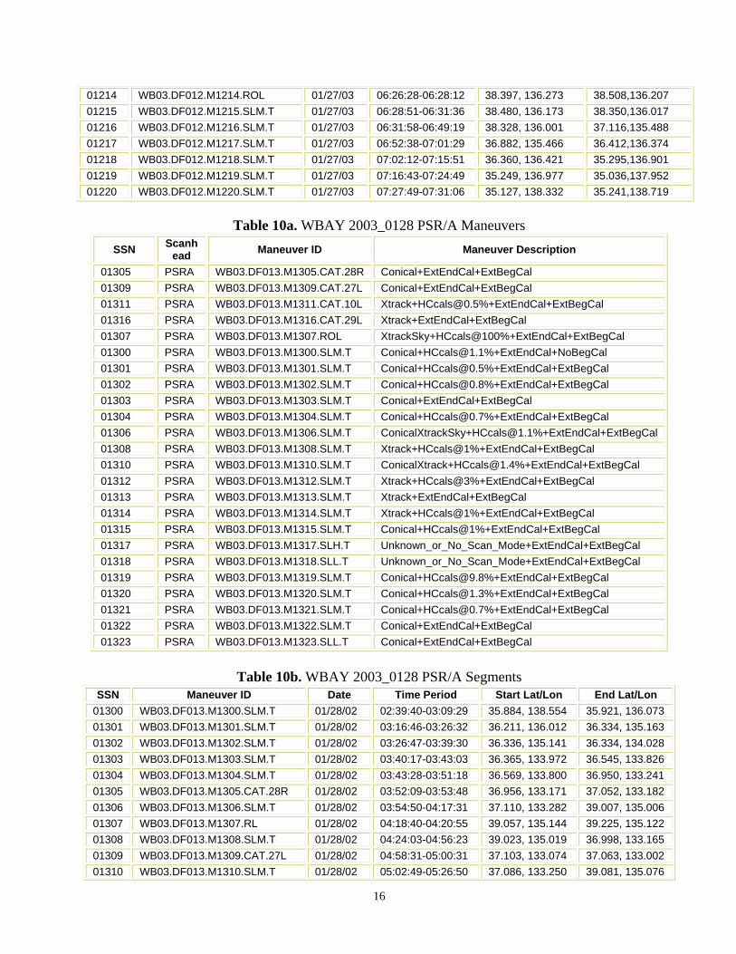
01214 WB03.DF012.M1214.ROL 01/27/03 06:26:28-06:28:12 38.397, 136.273 38.508,136.207 01215 WB03.DF012.M1215.SLM.T 01/27/03 06:28:51-06:31:36 38.480, 136.173 38.350,136.017 01216 WB03.DF012.M1216.SLM.T 01/27/03 06:31:58-06:49:19 38.328, 136.001 37.116,135.488 01217 WB03.DF012.M1217.SLM.T 01/27/03 06:52:38-07:01:29 36.882, 135.466 36.412,136.374 01218 WB03.DF012.M1218.SLM.T 01/27/03 07:02:12-07:15:51 36.360, 136.421 35.295,136.901 01219 WB03.DF012.M1219.SLM.T 01/27/03 07:16:43-07:24:49 35.249, 136.977 35.036,137.952 01220 WB03.DF012.M1220.SLM.T 01/27/03 07:27:49-07:31:06 35.127, 138.332 35.241,138.719
Table 10a. WBAY 2003_0128 PSR/A Maneuvers
SSN Scanhead Maneuver ID Maneuver Description
01305 PSRA WB03.DF013.M1305.CAT.28R Conical+ExtEndCal+ExtBegCal 01309 PSRA WB03.DF013.M1309.CAT.27L Conical+ExtEndCal+ExtBegCal 01311 PSRA WB03.DF013.M1311.CAT.10L [email protected]%+ExtEndCal+ExtBegCal 01316 PSRA WB03.DF013.M1316.CAT.29L Xtrack+ExtEndCal+ExtBegCal 01307 PSRA WB03.DF013.M1307.ROL XtrackSky+HCcals@100%+ExtEndCal+ExtBegCal 01300 PSRA WB03.DF013.M1300.SLM.T [email protected]%+ExtEndCal+NoBegCal 01301 PSRA WB03.DF013.M1301.SLM.T [email protected]%+ExtEndCal+ExtBegCal 01302 PSRA WB03.DF013.M1302.SLM.T [email protected]%+ExtEndCal+ExtBegCal 01303 PSRA WB03.DF013.M1303.SLM.T Conical+ExtEndCal+ExtBegCal 01304 PSRA WB03.DF013.M1304.SLM.T [email protected]%+ExtEndCal+ExtBegCal 01306 PSRA WB03.DF013.M1306.SLM.T [email protected]%+ExtEndCal+ExtBegCal 01308 PSRA WB03.DF013.M1308.SLM.T Xtrack+HCcals@1%+ExtEndCal+ExtBegCal 01310 PSRA WB03.DF013.M1310.SLM.T [email protected]%+ExtEndCal+ExtBegCal 01312 PSRA WB03.DF013.M1312.SLM.T Xtrack+HCcals@3%+ExtEndCal+ExtBegCal 01313 PSRA WB03.DF013.M1313.SLM.T Xtrack+ExtEndCal+ExtBegCal 01314 PSRA WB03.DF013.M1314.SLM.T Xtrack+HCcals@1%+ExtEndCal+ExtBegCal 01315 PSRA WB03.DF013.M1315.SLM.T Conical+HCcals@1%+ExtEndCal+ExtBegCal 01317 PSRA WB03.DF013.M1317.SLH.T Unknown_or_No_Scan_Mode+ExtEndCal+ExtBegCal 01318 PSRA WB03.DF013.M1318.SLL.T Unknown_or_No_Scan_Mode+ExtEndCal+ExtBegCal 01319 PSRA WB03.DF013.M1319.SLM.T [email protected]%+ExtEndCal+ExtBegCal 01320 PSRA WB03.DF013.M1320.SLM.T [email protected]%+ExtEndCal+ExtBegCal 01321 PSRA WB03.DF013.M1321.SLM.T [email protected]%+ExtEndCal+ExtBegCal 01322 PSRA WB03.DF013.M1322.SLM.T Conical+ExtEndCal+ExtBegCal 01323 PSRA WB03.DF013.M1323.SLL.T Conical+ExtEndCal+ExtBegCal
Table 10b. WBAY 2003_0128 PSR/A Segments
SSN Maneuver ID Date Time Period Start Lat/Lon End Lat/Lon 01300 WB03.DF013.M1300.SLM.T 01/28/02 02:39:40-03:09:29 35.884, 138.554 35.921, 136.073 01301 WB03.DF013.M1301.SLM.T 01/28/02 03:16:46-03:26:32 36.211, 136.012 36.334, 135.163 01302 WB03.DF013.M1302.SLM.T 01/28/02 03:26:47-03:39:30 36.336, 135.141 36.334, 134.028 01303 WB03.DF013.M1303.SLM.T 01/28/02 03:40:17-03:43:03 36.365, 133.972 36.545, 133.826 01304 WB03.DF013.M1304.SLM.T 01/28/02 03:43:28-03:51:18 36.569, 133.800 36.950, 133.241 01305 WB03.DF013.M1305.CAT.28R 01/28/02 03:52:09-03:53:48 36.956, 133.171 37.052, 133.182 01306 WB03.DF013.M1306.SLM.T 01/28/02 03:54:50-04:17:31 37.110, 133.282 39.007, 135.006 01307 WB03.DF013.M1307.RL 01/28/02 04:18:40-04:20:55 39.057, 135.144 39.225, 135.122 01308 WB03.DF013.M1308.SLM.T 01/28/02 04:24:03-04:56:23 39.023, 135.019 36.998, 133.165 01309 WB03.DF013.M1309.CAT.27L 01/28/02 04:58:31-05:00:31 37.103, 133.074 37.063, 133.002 01310 WB03.DF013.M1310.SLM.T 01/28/02 05:02:49-05:26:50 37.086, 133.250 39.081, 135.076
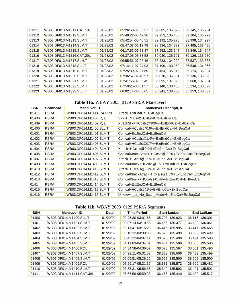
17
01311 WB03.DF013.M1311.CAT.10L 01/28/02 05:26:53-05:36:57 39.085, 135.079 39.145, 135.264 01312 WB03.DF013.M1312.SLM.T 01/28/02 05:40:22-05:42:36 39.252, 135.485 39.204, 135.292 01313 WB03.DF013.M1313.SLM.T 01/28/02 05:42:54-05:46:51 39.192, 135.270 38.998, 134.997 01314 WB03.DF013.M1314.SLM.T 01/28/02 05:47:03-06:12:49 38.986, 134.983 37.495, 133.496 01315 WB03.DF013.M1315.SLM.T 01/28/02 06:17:53-06:33:37 37.552, 133.547 38.849, 134.844 01316 WB03.DF013.M1316.CAT.29L 01/28/02 06:37:06-06:38:58 39.030, 135.191 39.126, 135.250 01317 WB03.DF013.M1317.SLH.T 01/28/02 06:55:56-07:08:16 38.233, 134.222 37.537, 133.536 01318 WB03.DF013.M1318.SLL.T 01/28/02 07:14:11-07:24:03 37.190, 133.950 36.548, 134.866 01319 WB03.DF013.M1319.SLM.T 01/28/02 07:25:30-07:34:59 36.464, 135.013 36.174, 136.224 01320 WB03.DF013.M1320.SLM.T 01/28/02 07:36:57-07:40:57 36.070, 136.394 36.136, 136.920 01321 WB03.DF013.M1321.SLM.T 01/28/02 07:41:56-07:55:45 36.095, 137.023 35.068, 137.954 01322 WB03.DF013.M1322.SLM.T 01/28/02 07:59:25-08:01:57 35.148, 138.405 35.234, 138.699 01323 WB03.DF013.M1323.SLL.T 01/28/02 08:02:14-08:03:05 35.241, 138.733 35.253, 138.837
Table 11a. WBAY 2003_0129 PSR/A Maneuvers
SSN Scanhead Maneuver ID Maneuver Descripti, n 01411 PSRA WB03.DF014.M1411.CAT.39L Xtrack+ExtEndCal+ExtBegCal 01406 PSRA WB03.DF014.M1406.R, L Sky+HCcals=2+ExtEndCal+ExtBegCal 01409 PSRA WB03.DF014.M1409.R, L XtrackSky+HCcals@300%+ExtEndCal+ExtBegCal 01400 PSRA WB03.DF014.M1400.SLL.T [email protected]%+ExtEndCal+N, BegCal 01401 PSRA WB03.DF014.M1401.SLM.T Conical+ExtEndCal+ExtBegCal 01402 PSRA WB03.DF014.M1402.SLM.T [email protected]%+ExtEndCal+ExtBegCal 01403 PSRA WB03.DF014.M1403.SLM.T [email protected]%+ExtEndCal+ExtBegCal 01404 PSRA WB03.DF014.M1404.SLM.T [email protected]%+ExtEndCal+ExtBegCal 01405 PSRA WB03.DF014.M1405.SLM.T [email protected]%+ExtEndCal+ExtBegCal 01407 PSRA WB03.DF014.M1407.SLM.T [email protected]%+ExtEndCal+ExtBegCal 01408 PSRA WB03.DF014.M1408.SLM.T ConicalXtrack+HCcals@1%+ExtEndCal+ExtBegCal 01410 PSRA WB03.DF014.M1410.SLM.T [email protected]%+ExtEndCal+ExtBegCal 01412 PSRA WB03.DF014.M1412.SLM.T [email protected]%+ExtEndCal+ExtBegCal 01413 PSRA WB03.DF014.M1413.SLM.T [email protected]%+ExtEndCal+ExtBegCal 01414 PSRA WB03.DF014.M1414.SLM.T Conical+ExtEndCal+ExtBegCal 01415 PSRA WB03.DF014.M1415.SLM.T Conical+HCcals@1%+ExtEndCal+ExtBegCal 01416 PSRA WB03.DF014.M1416.SLM.T Unknown_or_No_Scan_Mode+NoEndCal+ExtBegCal
Table 11b. WBAY 2003_0129 PSR/A Segments
SSN Maneuver ID Date Time Period Start Lat/Lon End Lat/Lon 01400 WB03.DF014.M1400.SLL.T 01/29/02 02:26:30-03:01:56 35.703, 139.023 36.116, 136.301 01401 WB03.DF014.M1401.SLM.T 01/29/02 03:07:14-03:10:55 36.456, 136.377 36.409, 136.061 01402 WB03.DF014.M1402.SLM.T 01/29/02 03:11:41-03:15:29 36.415, 135.995 36.417, 135.655 01403 WB03.DF014.M1403.SLM.T 01/29/02 03:18:12-03:39:03 36.570, 135.499 38.509, 135.499 01404 WB03.DF014.M1404.SLM.T 01/29/02 03:43:32-04:07:11 38.578, 135.498 36.494, 135.500 01405 WB03.DF014.M1405.SLM.T 01/29/02 04:11:03-04:34:01 36.454, 135.508 38.506, 135.500 01406 WB03.DF014.M1406.ROL 01/29/02 04:34:58-04:36:57 38.573, 135.567 38.661, 135.490 01407 WB03.DF014.M1407.SLM.T 01/29/02 04:38:11-05:01:52 38.558, 135.506 36.493, 135.499 01408 WB03.DF014.M1408.SLM.T 01/29/02 05:05:51-05:28:16 36.529, 135.500 38.509, 135.500 01409 WB03.DF014.M1409.ROL 01/29/02 05:29:17-05:31:37 38.581, 135.573 38.699, 135.482 01410 WB03.DF014.M1410.SLM.T 01/29/02 05:33:31-05:56:53 38.540, 135.503 36.491, 135.501 01411 WB03.DF014.M1411.CAT.39L 01/29/02 05:57:56-05:59:38 36.465, 135.440 36.439, 135.517
18
01412 WB03.DF014.M1412.SLM.T 01/29/02 06:00:49-06:04:45 36.525, 135.499 36.855, 135.500 01413 WB03.DF014.M1413.SLM.T 01/29/02 06:06:35-06:13:06 36.890, 135.684 36.446, 136.331 01414 WB03.DF014.M1414.SLM.T 01/29/02 06:14:37-06:17:24 36.326, 136.341 36.152, 136.203 01415 WB03.DF014.M1415.SLM.T 01/29/02 06:18:29-06:34:00 36.069, 136.247 35.058, 137.942 01416 WB03.DF014.M1416.SLM.T 01/29/02 06:37:48-06:39:57 35.164, 138.470 35.245, 138.738
Table 12a. WBAY 2003_0130 PSR/A Maneuvers
SSN Scanhead Maneuver ID Maneuver Description 01504 PSRA WB03.DF015.M1504.CAT.15L [email protected]%+ExtEndCal+ExtBegCal 01505 PSRA WB03.DF015.M1505.CAT.27L Xtrack+ExtEndCal+ExtBegCal 01508 PSRA WB03.DF015.M1508.CAT.15R [email protected]%+ExtEndCal+ExtBegCal 01509 PSRA WB03.DF015.M1509.CAT.15L [email protected]%+ExtEndCal+ExtBegCal 01513 PSRA WB03.DF015.M1513.CAT.20L Xtrack+ExtEndCal+ExtBegCal 01516 PSRA WB03.DF015.M1516.CAT.20R Xtrack+ExtEndCal+ExtBegCal 01511 PSRA WB03.DF015.M1511.ROL Sky+HCcals=2+ExtEndCal+ExtBegCal 01500 PSRA WB03.DF015.M1500.SLM.T [email protected]%+ExtEndCal+NoBegCal 01501 PSRA WB03.DF015.M1501.SLM.T [email protected]%+ExtEndCal+NoBegCal 01502 PSRA WB03.DF015.M1502.SLM.T [email protected]%+ExtEndCal+ExtBegCal 01503 PSRA WB03.DF015.M1503.SLM.T ConicalXtrack+HCcals@1%+ExtEndCal+ExtBegCal 01506 PSRA WB03.DF015.M1506.SLM.T [email protected]%+ExtEndCal+ExtBegCal 01507 PSRA WB03.DF015.M1507.SLM.T [email protected]%+ExtEndCal+ExtBegCal 01510 PSRA WB03.DF015.M1510.SLM.T [email protected]%+ExtEndCal+ExtBegCal 01512 PSRA WB03.DF015.M1512.SLM.T Xtrack+HCcals@1%+ExtEndCal+ExtBegCal 01514 PSRA WB03.DF015.M1514.SLM.T [email protected]%+ExtEndCal+ExtBegCal 01515 PSRA WB03.DF015.M1515.SLM.T Conical+HCcals@1%+ExtEndCal+ExtBegCal 01517 PSRA WB03.DF015.M1517.SLL.T [email protected]%+ExtEndCal+ExtBegCal 01518 PSRA WB03.DF015.M1518.SLM.T [email protected]%+ExtEndCal+ExtBegCal 01519 PSRA WB03.DF015.M1519.SLM.T [email protected]%+NoEndCal+ExtBegCal 01520 PSRA WB03.DF015.M1520.SLM.T No_Radiometric_Data
Table 12b. WBAY 2003_0130 PSR/A Segments
SSN Maneuver ID Date Time Period Start Lat/Lon End Lat/Lon 01500 WB03.DF015.M1500.SLM.T 01/30/02 02:17:20-02:21:18 35.959, 138.908 35.888, 138.584 01501 WB03.DF015.M1501.SLM.T 01/30/02 02:21:46-02:52:11 35.887, 138.542 36.206, 135.950 01502 WB03.DF015.M1502.SLM.T 01/30/02 02:54:57-03:09:53 36.175, 135.703 36.337, 134.450 01503 WB03.DF015.M1503.SLM.T 01/30/02 03:13:30-03:46:31 36.378, 134.543 38.731, 137.069 01504 WB03.DF015.M1504.CAT.15L 01/30/02 03:46:37-03:52:49 38.738, 137.076 38.675, 137.214 01505 WB03.DF015.M1505.CAT.27L 01/30/02 03:54:04-03:55:56 38.679, 137.361 38.749, 137.448 01506 WB03.DF015.M1506.SLM.T 01/30/02 03:56:06-03:59:13 38.750, 137.434 38.731, 137.171 01507 WB03.DF015.M1507.SLM.T 01/30/02 04:01:08-04:42:24 38.677, 137.015 36.316, 134.482 01508 WB03.DF015.M1508.CAT.15R 01/30/02 04:42:27-04:43:58 36.314, 134.479 36.319, 134.375 01509 WB03.DF015.M1509.CAT.15L 01/30/02 04:44:30-04:50:21 36.350, 134.351 36.291, 134.522 01510 WB03.DF015.M1510.SLM.T 01/30/02 04:51:11-05:24:08 36.352, 134.526 38.672, 137.006 01511 WB03.DF015.M1511.R, L 01/30/02 05:25:01-05:26:55 38.709, 137.103 38.790, 137.051 01512 WB03.DF015.M1512.SLM.T 01/30/02 05:30:43-06:03:56 38.548, 136.874 36.665, 134.841 01513 WB03.DF015.M1513.CAT.20L 01/30/02 06:06:05-06:09:30 36.703, 134.699 36.588, 134.801 01514 WB03.DF015.M1514.SLM.T 01/30/02 06:09:32-06:12:22 36.590, 134.803 36.759, 135.063 01515 WB03.DF015.M1515.SLM.T 01/30/02 06:23:00-06:39:35 37.032, 135.242 38.215, 136.465 01516 WB03.DF015.M1516.CAT.20R 01/30/02 06:39:42-06:41:55 38.223, 136.474 38.152, 136.676
19
01517 WB03.DF015.M1517.SLL.T 01/30/02 06:41:58-06:56:16 38.147, 136.675 36.931, 136.392 01518 WB03.DF015.M1518.SLM.T 01/30/02 07:06:58-07:14:08 35.992, 136.370 35.303, 136.887 01519 WB03.DF015.M1519.SLM.T 01/30/02 07:15:00-07:20:33 35.247, 136.991 35.076, 137.777 01520 WB03.DF015.M1520.SLM.T 01/30/02 07:26:33-07:29:12 35.160, 138.444 35.234, 138.699
Table 13a. WBAY 2003_0201 PSR/A Maneuvers
SSN Scanhead Maneuver ID Maneuver Description 01602 PSRA WB03.DF016.M1602.ROL Sky+HCcals=2+ExtEndCal+ExtBegCal 01600 PSRA WB03.DF016.M1600.SLM.T [email protected]%+ExtEndCal+NoBegCal 01601 PSRA WB03.DF016.M1601.SLM.T [email protected]%+ExtEndCal+ExtBegCal 01603 PSRA WB03.DF016.M1603.SLL.T Conical+ExtEndCal+ExtBegCal 01604 PSRA WB03.DF016.M1604.SLL.T [email protected]%+ExtEndCal+ExtBegCal 01605 PSRA WB03.DF016.M1605.SLL.T [email protected]%+NoEndCal+ExtBegCal 01606 PSRA WB03.DF016.M1606.SLL.T No_Radiometric_Data
Table 13b. WBAY 2003_0201 PSR/A Segments
SSN Maneuver ID Date Time Period Start Lat/Lon End Lat/Lon 01600 WB03.DF016.M1600.SLM.T 02/01/03 03:27:45-03:54:41 35.884, 138.552 35.921, 136.074 01601 WB03.DF016.M1601.SLM.T 02/01/03 03:58:41-04:01:07 36.205, 136.251 36.402, 136.411 01602 WB03.DF016.M1602.R, L 02/01/03 04:01:44-04:03:31 36.441, 136.472 36.547, 136.439 01603 WB03.DF016.M1603.SLL.T 02/01/03 04:06:23-04:08:42 36.349, 136.369 36.202, 136.243 01604 WB03.DF016.M1604.SLL.T 02/01/03 04:13:02-04:24:41 35.988, 136.538 35.179, 137.762 01605 WB03.DF016.M1605.SLL.T 02/01/03 04:30:06-04:33:09 35.214, 138.447 35.281, 138.788 01606 WB03.DF016.M1606.SLL.T 02/01/03 04:40:48-04:43:34 35.445, 139.413 35.567, 139.391
Table 14a. WBAY 2003_0203 PSR/A Maneuvers
SSN Scanhead Maneuver ID Maneuver Description 01705 PSRA WB03.DF017.M1705.CAT.10R [email protected]%+ExtEndCal+ExtBegCal 01706 PSRA WB03.DF017.M1706.CAT.10L [email protected]%+ExtEndCal+ExtBegCal 01709 PSRA WB03.DF017.M1709.CAT.29L Xtrack+HCcals@45%+ExtEndCal+ExtBegCal 01712 PSRA WB03.DF017.M1712.CAT.30L [email protected]%+ExtEndCal+ExtBegCal 01717 PSRA WB03.DF017.M1717.CAT.28L [email protected]%+ExtEndCal+ExtBegCal 01711 PSRA WB03.DF017.M1711.ROL [email protected]%+ExtEndCal+ExtBegCal 01700 PSRA WB03.DF017.M1700.SLL.T [email protected]%+ExtEndCal+NoBegCal 01701 PSRA WB03.DF017.M1701.SLL.T Conical+HCcals@2%+ExtEndCal+NoBegCal 01702 PSRA WB03.DF017.M1702.SLL.T [email protected]%+ExtEndCal+ExtBegCal 01703 PSRA WB03.DF017.M1703.SLL.T [email protected]%+ExtEndCal+ExtBegCal 01704 PSRA WB03.DF017.M1704.SLM.T [email protected]%+ExtEndCal+ExtBegCal 01707 PSRA WB03.DF017.M1707.SLM.T [email protected]%+ExtEndCal+ExtBegCal 01708 PSRA WB03.DF017.M1708.SLM.T [email protected]%+ExtEndCal+ExtBegCal 01710 PSRA WB03.DF017.M1710.SLM.T [email protected]%+ExtEndCal+ExtBegCal 01713 PSRA WB03.DF017.M1713.SLL.T [email protected]%+ExtEndCal+ExtBegCal 01714 PSRA WB03.DF017.M1714.SLL.T Xtrack+ExtEndCal+ExtBegCal 01715 PSRA WB03.DF017.M1715.SLL.T Xtrack+ExtEndCal+ExtBegCal 01716 PSRA WB03.DF017.M1716.SLL.T Xtrack+ExtEndCal+ExtBegCal 01718 PSRA WB03.DF017.M1718.SLM.T [email protected]%+ExtEndCal+ExtBegCal 01719 PSRA WB03.DF017.M1719.SLL.T No_Radiometric_Data 01720 PSRA WB03.DF017.M1720.SLL.T No_Radiometric_Data
20
Table 14b. WBAY 2003_0203 PSR/A Segments
01700 WB03.DF017.M1700.SLL.T 02/03/03 02:07:51-02:15:17 35.572, 139.406 34.986, 139.399 01701 WB03.DF017.M1701.SLL.T 02/03/03 02:19:47-02:22:34 34.660, 139.403 34.444, 139.462 01702 WB03.DF017.M1702.SLL.T 02/03/03 02:28:18-02:35:32 34.028, 139.571 33.428, 139.786 01703 WB03.DF017.M1703.SLL.T 02/03/03 02:38:50-03:03:12 33.166, 139.888 31.076, 140.678 01704 WB03.DF017.M1704.SLM.T 02/03/03 03:04:33-03:22:12 31.001, 140.788 30.999, 143.042 01705 WB03.DF017.M1705.CAT.10R 02/03/03 03:22:16-03:24:54 30.998, 143.049 30.843, 143.276 01706 WB03.DF017.M1706.CAT.10L 02/03/03 03:25:04-03:32:58 30.830, 143.279 31.000, 143.683 01707 WB03.DF017.M1707.SLM.T 02/03/03 03:34:08-03:41:14 31.055, 143.610 31.405, 143.127 01708 WB03.DF017.M1708.SLM.T 02/03/03 03:43:59-04:00:40 31.607, 143.003 33.161, 142.993 01709 WB03.DF017.M1709.CAT.29L 02/03/03 04:00:45-04:02:25 33.169, 142.992 33.150, 142.919 01710 WB03.DF017.M1710.SLM.T 02/03/03 04:04:04-04:27:47 33.029, 142.998 30.988, 142.999 01711 WB03.DF017.M1711.ROL 02/03/03 04:28:36-04:31:20 30.934, 142.968 30.940, 143.154 01712 WB03.DF017.M1712.CAT.30L 02/03/03 04:32:28-04:51:31 31.009, 143.096 30.961, 143.026 01713 WB03.DF017.M1713.SLL.T 02/03/03 04:52:37-05:03:46 31.023, 143.004 31.785, 143.000 01714 WB03.DF017.M1714.SLL.T 02/03/03 05:07:23-05:09:50 32.045, 142.987 32.227, 143.000 01715 WB03.DF017.M1715.SLL.T 02/03/03 05:10:02-05:14:54 32.240, 143.001 32.579, 143.084 01716 WB03.DF017.M1716.SLL.T 02/03/03 05:17:49-05:21:27 32.767, 143.000 33.017, 143.000 01717 WB03.DF017.M1717.CAT.28L 02/03/03 05:22:05-05:41:55 33.055, 142.973 33.004, 142.987 01718 WB03.DF017.M1718.SLM.T 02/03/03 05:45:13-05:58:27 32.979, 143.021 33.890, 142.176 01719 WB03.DF017.M1719.SLL.T 02/03/03 06:15:53-06:24:46 34.579, 140.739 34.895, 140.082 01720 WB03.DF017.M1720.SLL.T 02/03/03 06:27:58-06:32:08 35.002, 139.862 35.191, 139.624
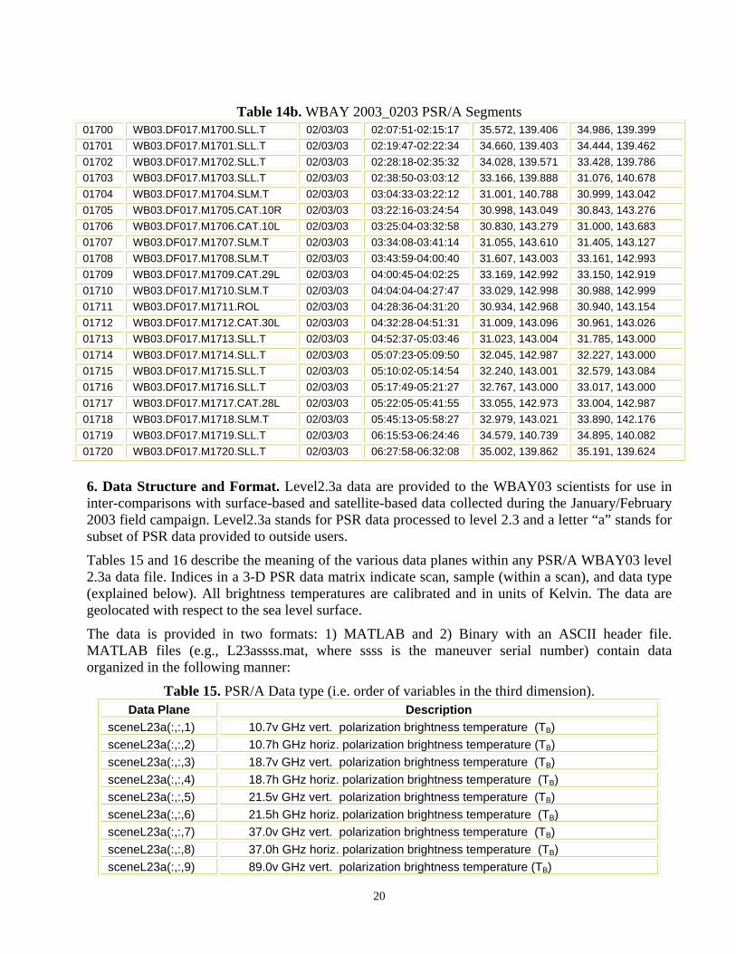
6. Data Structure and Format. Level2.3a data are provided to the WBAY03 scientists for use in inter-comparisons with surface-based and satellite-based data collected during the January/February 2003 field campaign. Level2.3a stands for PSR data processed to level 2.3 and a letter “a” stands for subset of PSR data provided to outside users.
Tables 15 and 16 describe the meaning of the various data planes within any PSR/A WBAY03 level 2.3a data file. Indices in a 3-D PSR data matrix indicate scan, sample (within a scan), and data type (explained below). All brightness temperatures are calibrated and in units of Kelvin. The data are geolocated with respect to the sea level surface.
The data is provided in two formats: 1) MATLAB and 2) Binary with an ASCII header file. MATLAB files (e.g., L23assss.mat, where ssss is the maneuver serial number) contain data organized in the following manner:
Table 15. PSR/A Data type (i.e. order of variables in the third dimension). Data Plane Description
sceneL23a(:,:,1) 10.7v GHz vert. polarization brightness temperature (TB) sceneL23a(:,:,2) 10.7h GHz horiz. polarization brightness temperature (TB) sceneL23a(:,:,3) 18.7v GHz vert. polarization brightness temperature (TB) sceneL23a(:,:,4) 18.7h GHz horiz. polarization brightness temperature (TB) sceneL23a(:,:,5) 21.5v GHz vert. polarization brightness temperature (TB) sceneL23a(:,:,6) 21.5h GHz horiz. polarization brightness temperature (TB) sceneL23a(:,:,7) 37.0v GHz vert. polarization brightness temperature (TB) sceneL23a(:,:,8) 37.0h GHz horiz. polarization brightness temperature (TB) sceneL23a(:,:,9) 89.0v GHz vert. polarization brightness temperature (TB)
21
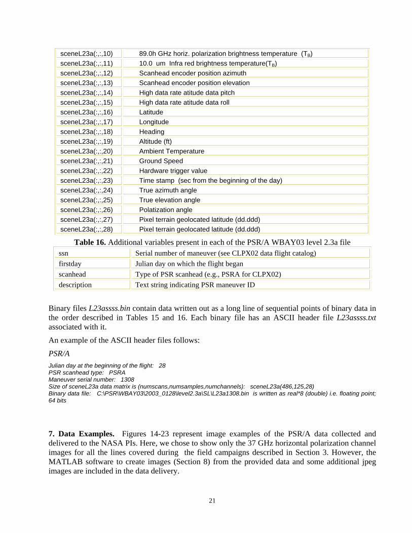
sceneL23a(:,:,10) 89.0h GHz horiz. polarization brightness temperature (TB) sceneL23a(:,:,11) 10.0 um Infra red brightness temperature(TB) sceneL23a(:,:,12) Scanhead encoder position azimuth sceneL23a(:,:,13) Scanhead encoder position elevation sceneL23a(:,:,14) High data rate atitude data pitch sceneL23a(:,:,15) High data rate atitude data roll sceneL23a(:,:,16) Latitude sceneL23a(:,:,17) Longitude sceneL23a(:,:,18) Heading sceneL23a(:,:,19) Altitude (ft) sceneL23a(:,:,20) Ambient Temperature sceneL23a(:,:,21) Ground Speed sceneL23a(:,:,22) Hardware trigger value sceneL23a(:,:,23) Time stamp (sec from the beginning of the day) sceneL23a(:,:,24) True azimuth angle sceneL23a(:,:,25) True elevation angle sceneL23a(:,:,26) Polatization angle sceneL23a(:,:,27) Pixel terrain geolocated latitude (dd.ddd) sceneL23a(:,:,28) Pixel terrain geolocated latitude (dd.ddd)
Table 16. Additional variables present in each of the PSR/A WBAY03 level 2.3a file ssn Serial number of maneuver (see CLPX02 data flight catalog) firstday Julian day on which the flight began scanhead Type of PSR scanhead (e.g., PSRA for CLPX02) description Text string indicating PSR maneuver ID
Binary files L23assss.bin contain data written out as a long line of sequential points of binary data in the order described in Tables 15 and 16. Each binary file has an ASCII header file L23assss.txt associated with it.
An example of the ASCII header files follows:
PSR/A Julian day at the beginning of the flight: 28 PSR scanhead type: PSRA Maneuver serial number: 1308 Size of sceneL23a data matrix is (numscans,numsamples,numchannels): sceneL23a(486,125,28) Binary data file: C:\PSR\WBAY03\2003_0128\level2.3a\SL\L23a1308.bin is written as real*8 (double) i.e. floating point; 64 bits
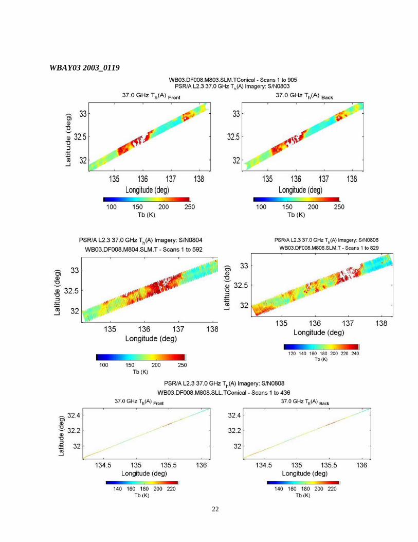
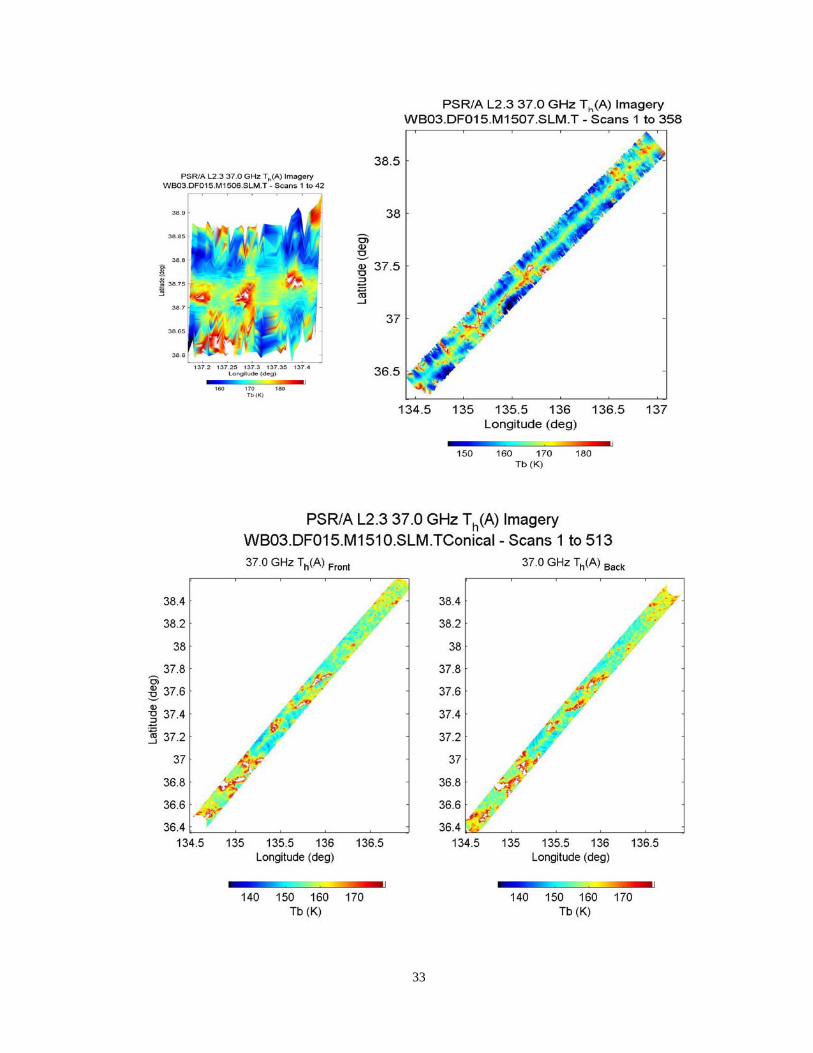
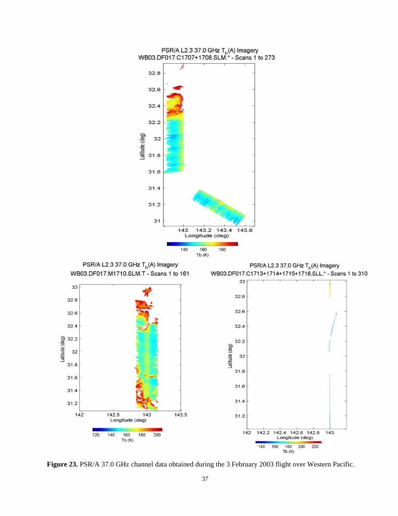
7. Data Examples. Figures 14-23 represent image examples of the PSR/A data collected and delivered to the NASA PIs. Here, we chose to show only the 37 GHz horizontal polarization channel images for all the lines covered during the field campaigns described in Section 3. However, the MATLAB software to create images (Section 8) from the provided data and some additional jpeg images are included in the data delivery.
22
WBAY03 2003_0119
23
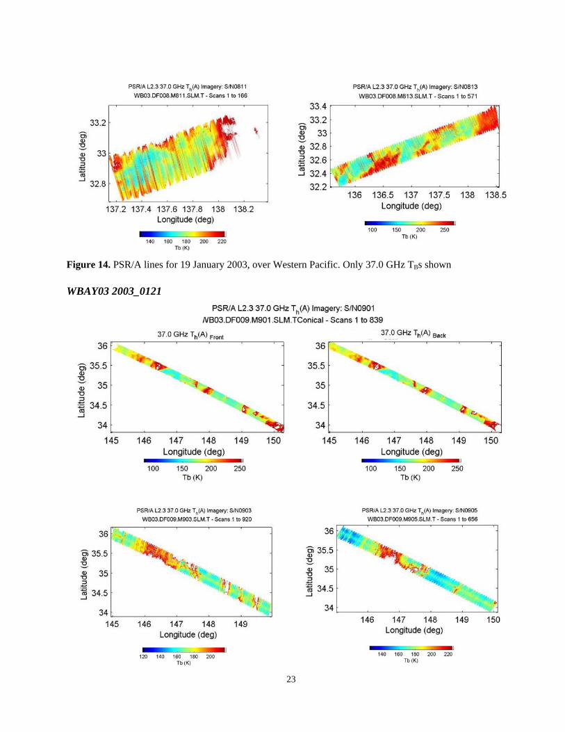
Figure 14. PSR/A lines for 19 January 2003, over Western Pacific. Only 37.0 GHz TBs shown
WBAY03 2003_0121
24
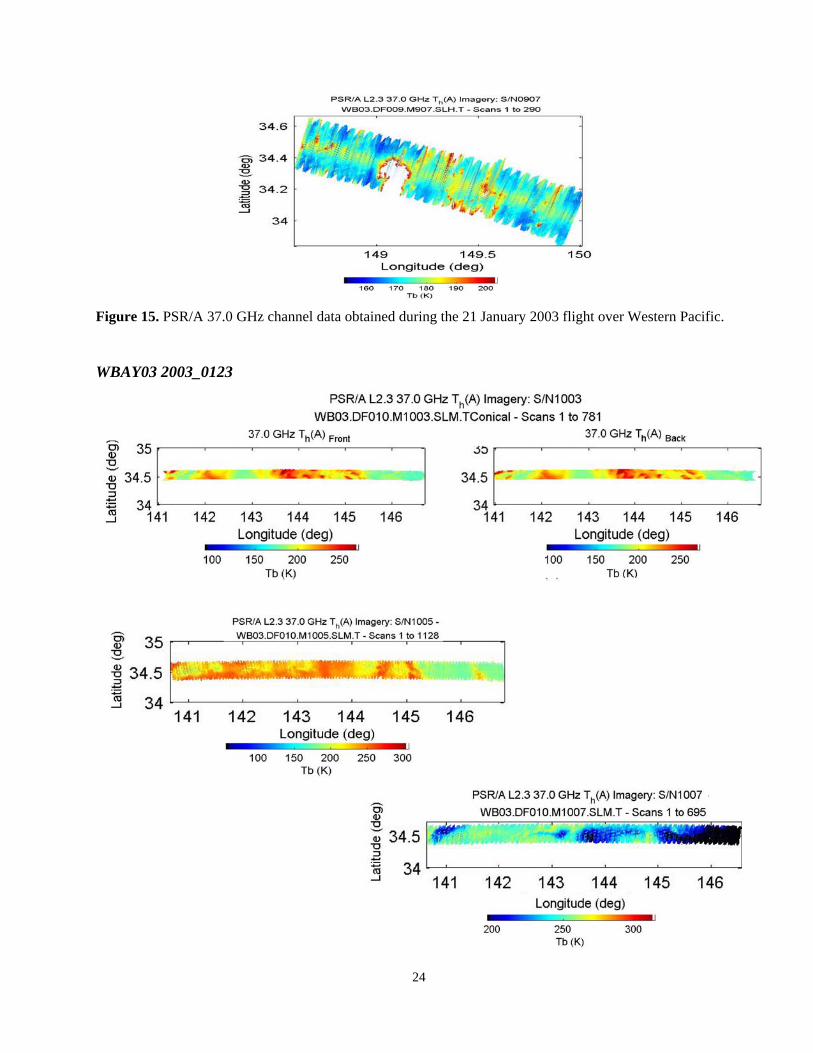
Figure 15. PSR/A 37.0 GHz channel data obtained during the 21 January 2003 flight over Western Pacific.
WBAY03 2003_0123
25
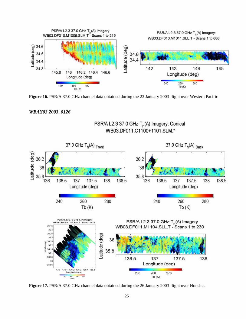
Figure 16. PSR/A 37.0 GHz channel data obtained during the 23 January 2003 flight over Western Pacific
WBAY03 2003_0126
Figure 17. PSR/A 37.0 GHz channel data obtained during the 26 January 2003 flight over Honshu.
26
WBAY03 2003_0127
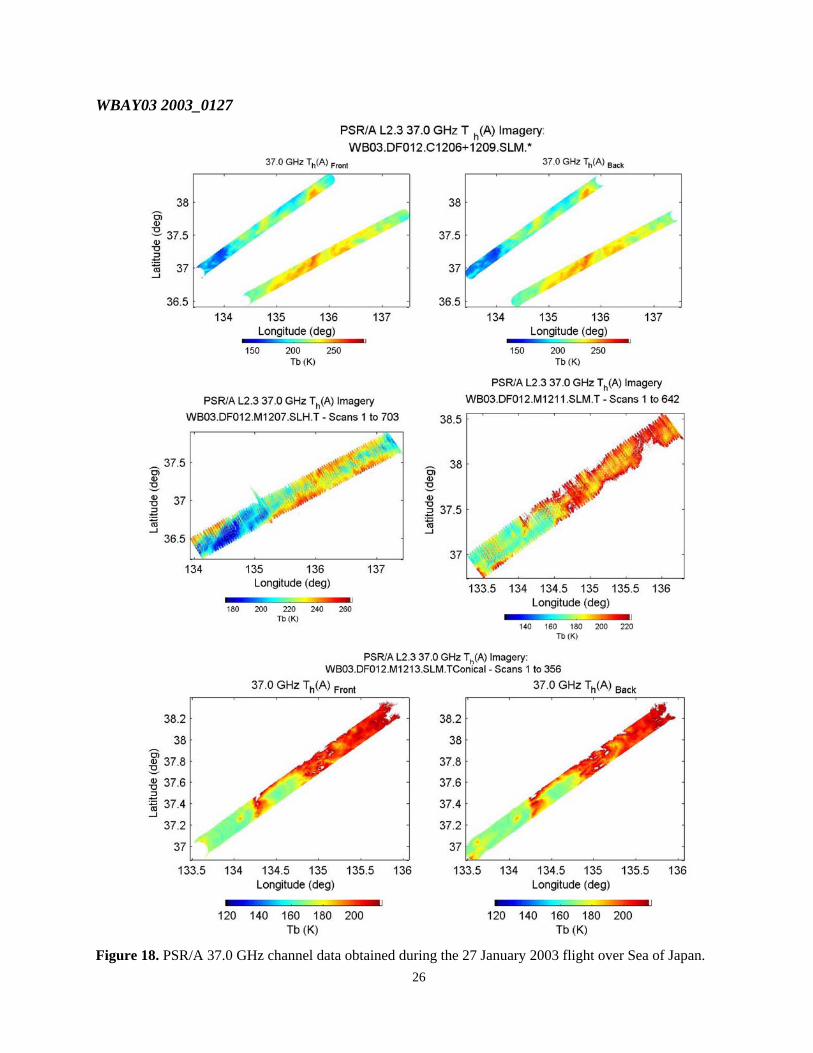
Figure 18. PSR/A 37.0 GHz channel data obtained during the 27 January 2003 flight over Sea of Japan.
27
WBAY03 2003_0128
28
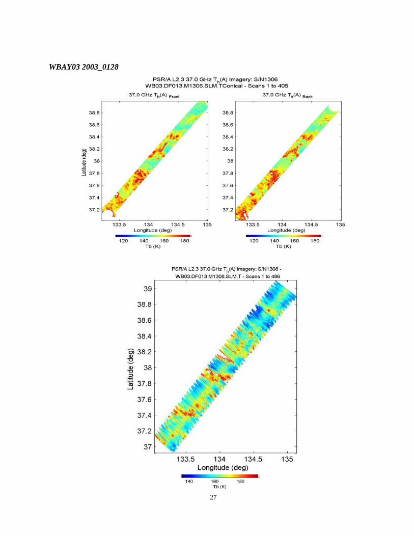
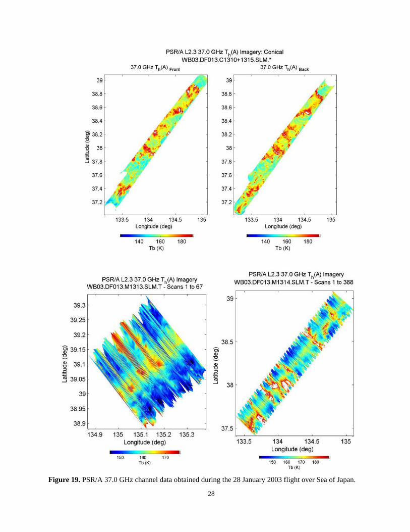
Figure 19. PSR/A 37.0 GHz channel data obtained during the 28 January 2003 flight over Sea of Japan.
29
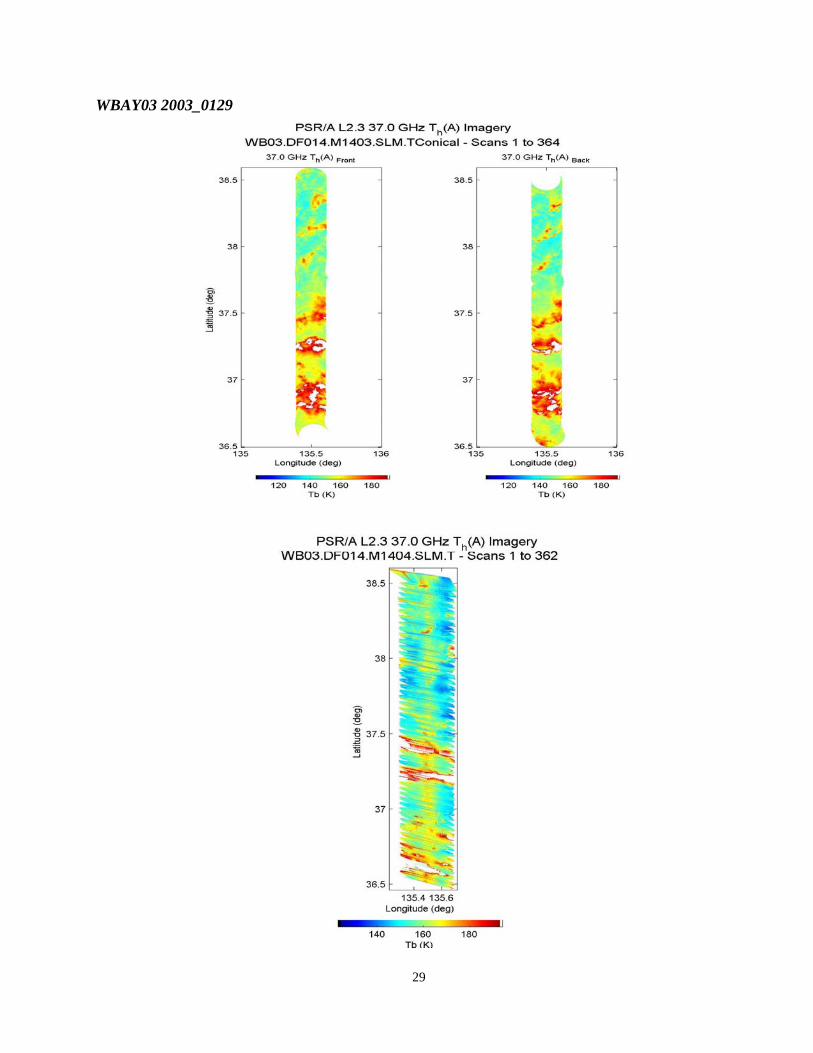
WBAY03 2003_0129
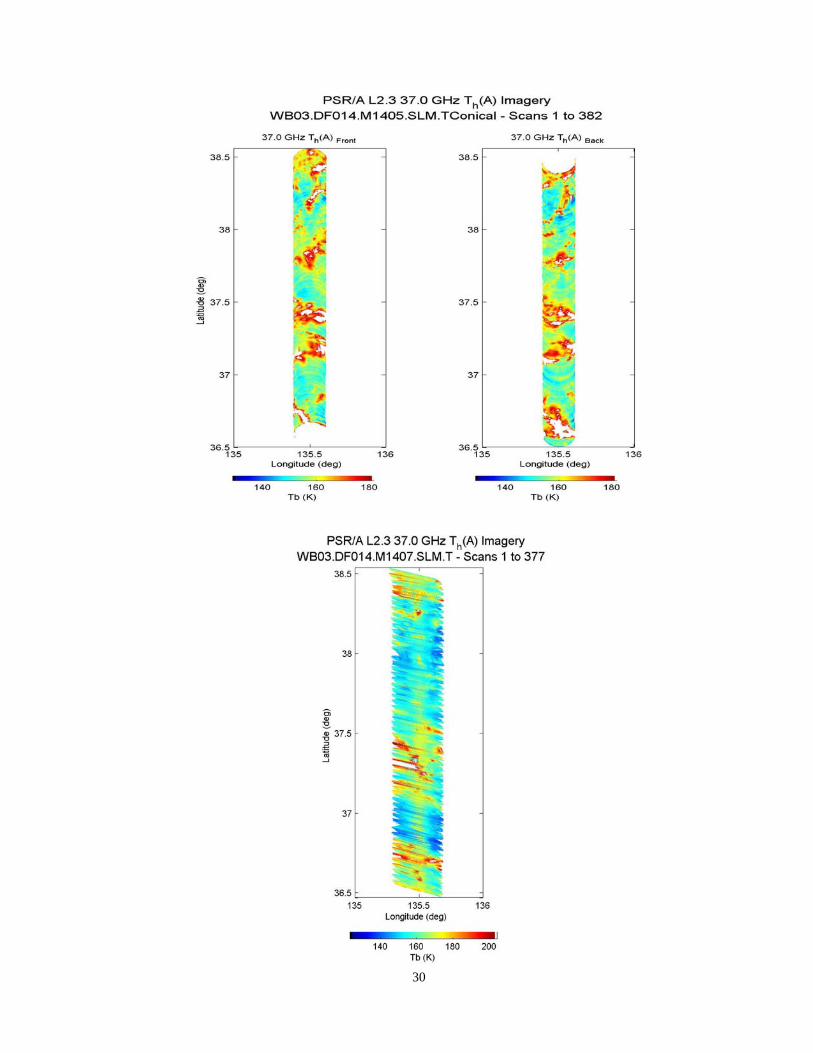
30
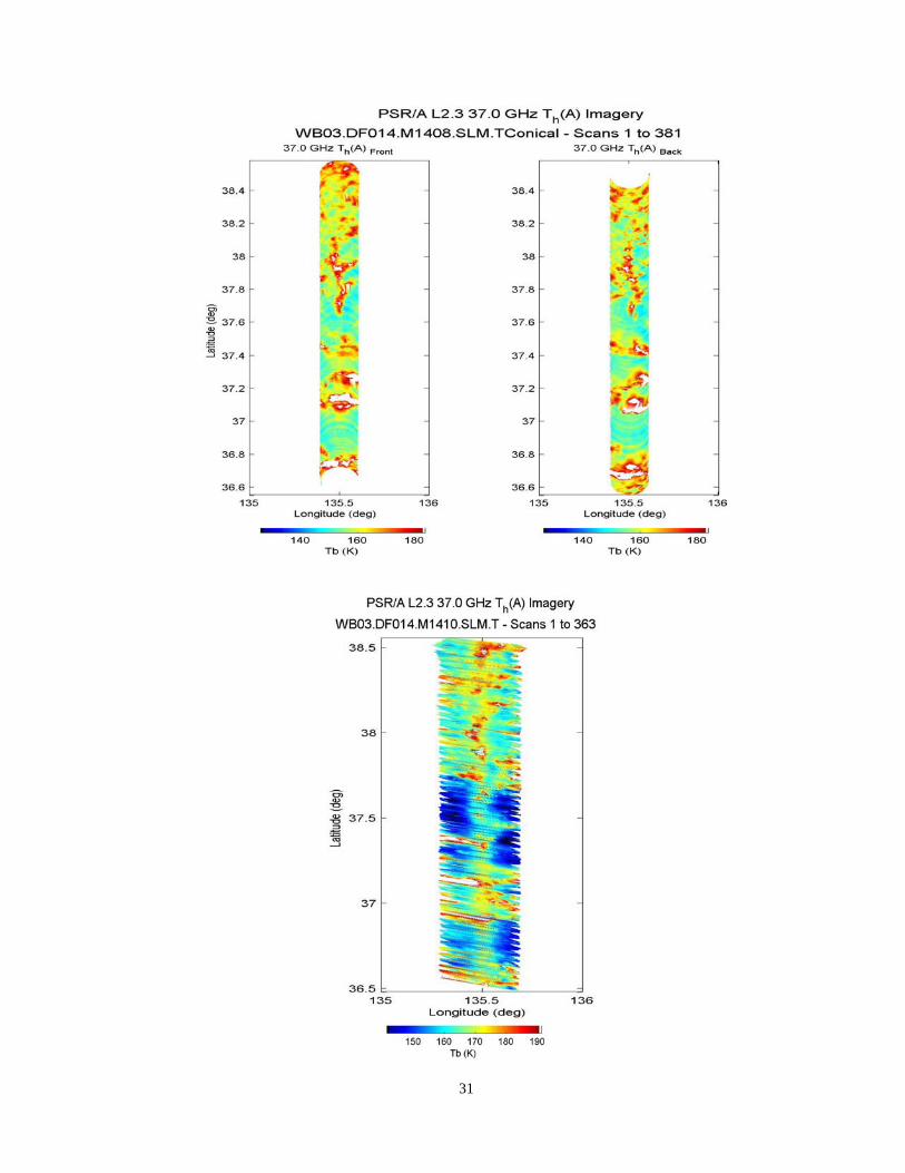
31
32
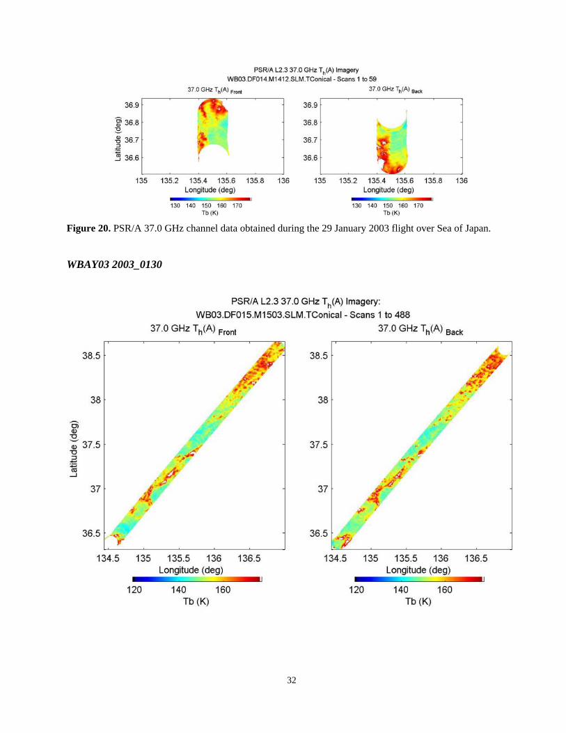
Figure 20. PSR/A 37.0 GHz channel data obtained during the 29 January 2003 flight over Sea of Japan.
WBAY03 2003_0130
33
34
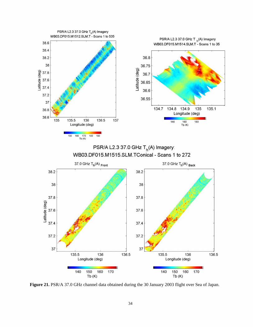
Figure 21. PSR/A 37.0 GHz channel data obtained during the 30 January 2003 flight over Sea of Japan.
35
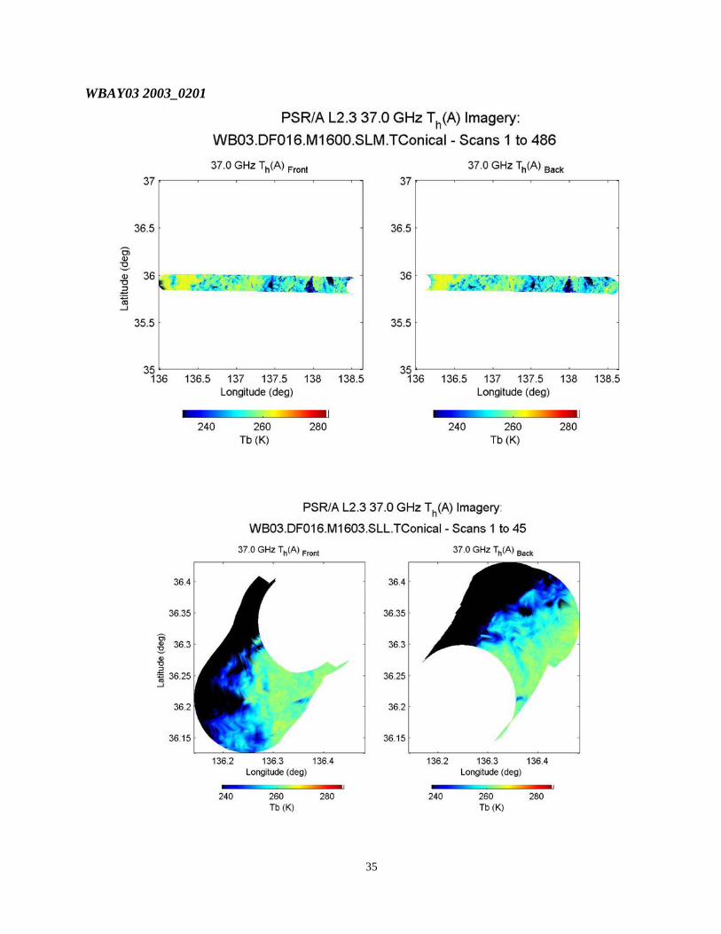
WBAY03 2003_0201
36
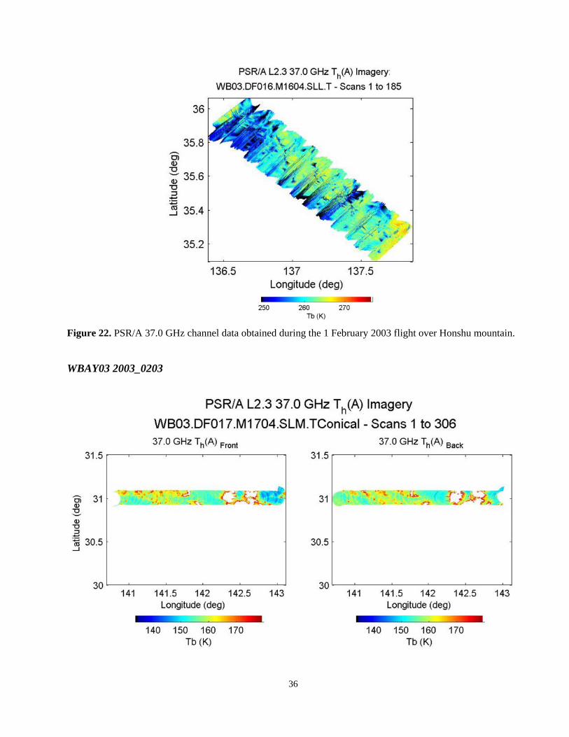
Figure 22. PSR/A 37.0 GHz channel data obtained during the 1 February 2003 flight over Honshu mountain.
WBAY03 2003_0203
37
Figure 23. PSR/A 37.0 GHz channel data obtained during the 3 February 2003 flight over Western Pacific.
38
8. MATLAB Software and Directory Structure for Displaying PSR/A Data. To enable the PSR/A data users to quickly view provided data, we included with the data a folder “display_l23a” that contains MATLAB version 6.1 m-files necessary to render brightness temperature maps from the PSR/A, level 2.3a data. We also included a MATLAB file “ReadBinL23aFile.m” which is an example of how to read binary and text files assuming that this will aid the user in designing their own data-reading routine using their software of choice. The calibrated 2.3a data are assumed to be organized in a series of subdirectories with the top one being the experiment directory. Thus, we have:
experiment_directory\yyyy_mmdd\level2.3a\sl\ where: “experiment_directory” is the root name of the main directory (e.g. WBAY03), “yyyy_mmdd” is a subdirectory indicating the year, month, and day of data, “level2.3a” is a subdirectory referring to the data level, “sl” is a subdirectly referring to straight and level maneuvers. “L23axxxx.mat” is a data file of type “.mat” i.e. MATLAB, corresponding to a maneuver with
serial number xxxx. “L23axxxx.bin” is a binary data file corresponding to a maneuver with serial number xxxx. It
contains data identical to the data contained in “.mat” file and is associated with header file “L23axxxx.txt”
Information pertaining to each individual maneuver can be found in Section 5 of this document.
MATLAB data and m-files are organized as described above. The user should create a PSR directory on their computer and copy the content of ETL Web files into this directory. The following two steps should be done next:
1) the m-file named “setrootdir.m” needs to be edited, with the variable “rootdir” changed to indicate the path to the directory “experiment_directory” , and
2) the MATLAB path needs to be modified (appended) using the “set path” command to include the subdirectory of mfiles contained in “display_23a”.
To run the display m-files a log file “WBAY03L23a.log” should be located in the “experiment_directory”. Issuing the command “mapl23a” in the Matlab command window will start the display code. The program will first ask which scanhead do you want and then it will show the available dates for display. The program then lists all available maneuvers from the selected flight code by their serial numbers and queries the user to select which file(s) is(are) to be displayed. The user can select the maneuver(s) by either the listed ordinal number or the associated WBAY03 maneuver serial number, for example, “sxxxx”. A group of maneuvers can be selected by indicating the range of ordinal numbers, for example, “2:13”. If more than one maneuver is selected, the program will ask if user wants to spatially interpolate between adjacent maneuvers (e.g., using kridging) or overlay them on top of each other. If interpolation is selected, the program will automatically interpolate between the end of one maneuver and beginning of the next. When the default option (overlay) is selected, no interpolation is performed and the data are overlaid, possibly overwriting data from previous maneuvers.
After loading data for selected maneuvers, the program queries the user for the channel (or set of channels) to be displayed. Several channel grouping options are provided in the command line. The next variables that can be selected are the minimum and maximum brightness temperatures for the range of the color map. If the minimum color temperature is defined by user, he/she will also be
39
asked for the maximum, otherwise the program will automatically assign those values. If auto-range calculation is selected the program will attempt to fit a Gaussian probability distribution function to the brightness temperature histogram, and compute the color range individually for each channel using the Gaussian parameters along with a range factor. The range factor sets the color range relative to the mean by the indicated number of standard deviations. The range factor defaults to 0.6, but can be modified according to the needs of the user. Autocorrelation is useful for scenes wherein the brightness temperatures mostly fall within a narrow range of values.
Proceeding, the user is able to display only a portion of the maneuver by selecting the scans to be displayed from all the scans available in the selected set of maneuvers. Here, for conical scanning, one full scan means one full rotation around azimuth axis, and includes front and back looks. Next, the user can choose to produce either individual maps (i.e., one image for each channel) or composite image of all channels and looks in a single map. Finally, the user has the option of selecting new latitude and longitude corners. If the user has installed the MATLAB Mapping Toolbox, he/she will also be asked to choose whether to include lines of individual U.S. states on the final map. Finally, we also provide a function “save_figures.m” that will save displayed figures in jpeg mode.
Related Documents