» Proton Polarimetry with the Hydrogen Jet Target at · PDF file» Proton Polarimetry with the Hydrogen Jet Target at ... o New asymmetries from elastic proton-heavy-ion scattering

» Proton Polarimetry with the Hydrogen Jet Target at

RHIC in Run 2015«

Oleg Eyserfor the RHIC Polarimetry Group

22nd International Spin SymposiumUniversity of Illinois, Urbana-Champaign

September 26-30, 2016

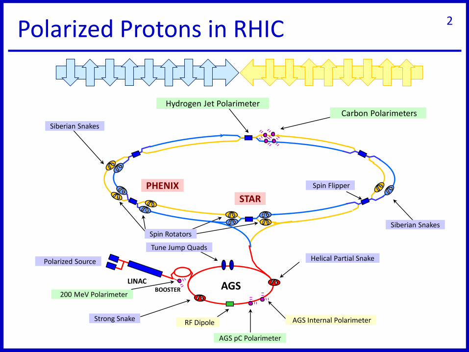
Polarized Protons in RHIC 2

AGSLINAC

BOOSTER

Polarized Source

200 MeV Polarimeter

Hydrogen Jet Polarimeter

PHENIX

STAR

Siberian Snakes

Siberian Snakes

Carbon Polarimeters

RF Dipole AGS Internal Polarimeter

AGS pC Polarimeter

Strong Snake

Tune Jump Quads

Helical Partial Snake

Spin Rotators

Spin Flipper

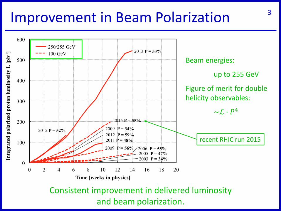
Improvement in Beam Polarization 3

Consistent improvement in delivered luminosity and beam polarization.

Beam energies:

up to 255 GeV

Figure of merit for double helicity observables:

~ℒ ⋅ 𝑃4

recent RHIC run 2015

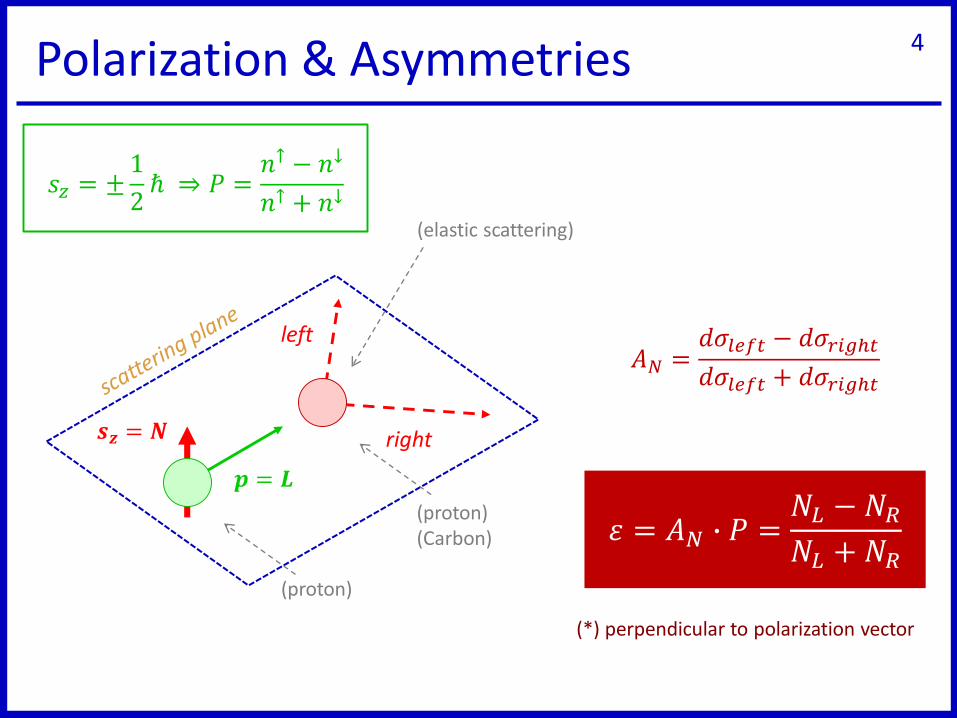
𝐴𝑁 =𝑑𝜎𝑙𝑒𝑓𝑡 − 𝑑𝜎𝑟𝑖𝑔ℎ𝑡

𝑑𝜎𝑙𝑒𝑓𝑡 + 𝑑𝜎𝑟𝑖𝑔ℎ𝑡

휀 = 𝐴𝑁 ∙ 𝑃 =𝑁𝐿 − 𝑁𝑅𝑁𝐿 + 𝑁𝑅

𝒔𝒛 = 𝑵

𝒑 = 𝑳

left

right

𝑠𝑧 = ±1

2ℏ ⇒ 𝑃 =

𝑛↑ − 𝑛↓

𝑛↑ + 𝑛↓

(proton)

(proton)(Carbon)

Polarization & Asymmetries 4

(*) perpendicular to polarization vector

(elastic scattering)

Carbon polarimeters

Two per ring

Fast measurement

𝛿𝑃/𝑃 ≈ 4%

Beam polarization profile

Polarization decay (time dependence)

Hydrogen jet polarimeter

Polarized target

Continuous operation

𝛿𝑃/𝑃 ≈ 5 − 8% per fill

normalization

5

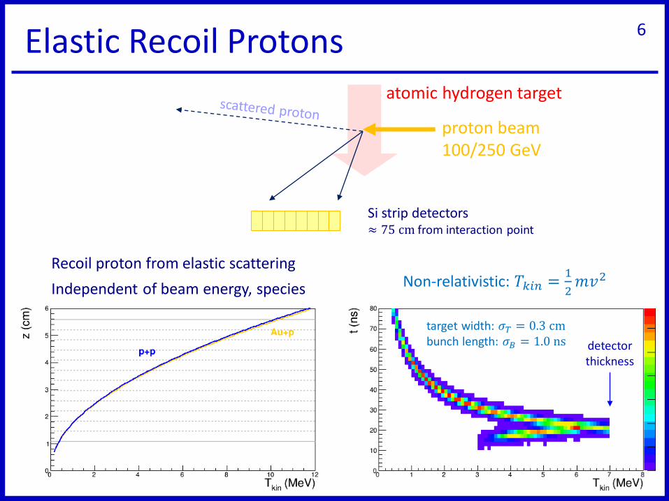
atomic hydrogen target

proton beam100/250 GeV

Si strip detectors≈ 75 cm from interaction point

Recoil proton from elastic scattering

Independent of beam energy, species

Elastic Recoil Protons 6

Non-relativistic: 𝑇𝑘𝑖𝑛 =1

2𝑚𝑣2

detectorthickness

target width: 𝜎𝑇 = 0.3 cmbunch length: 𝜎𝐵 = 1.0 ns

Detector Setup 7

INNER OUTER≈1

0 cm

12 strips3.75 mm each

75 cm

Set of eight Hamamatsu Si strip detectors

12 strips, each 3.75 mm wide, 500 μm thick

Uniform dead layer ≈ 1.5 μm

≈ 0.7 cm

𝑇𝑘𝑖𝑛 (MeV)

𝛿 𝐴𝐷𝐶(a.u.)

example detector

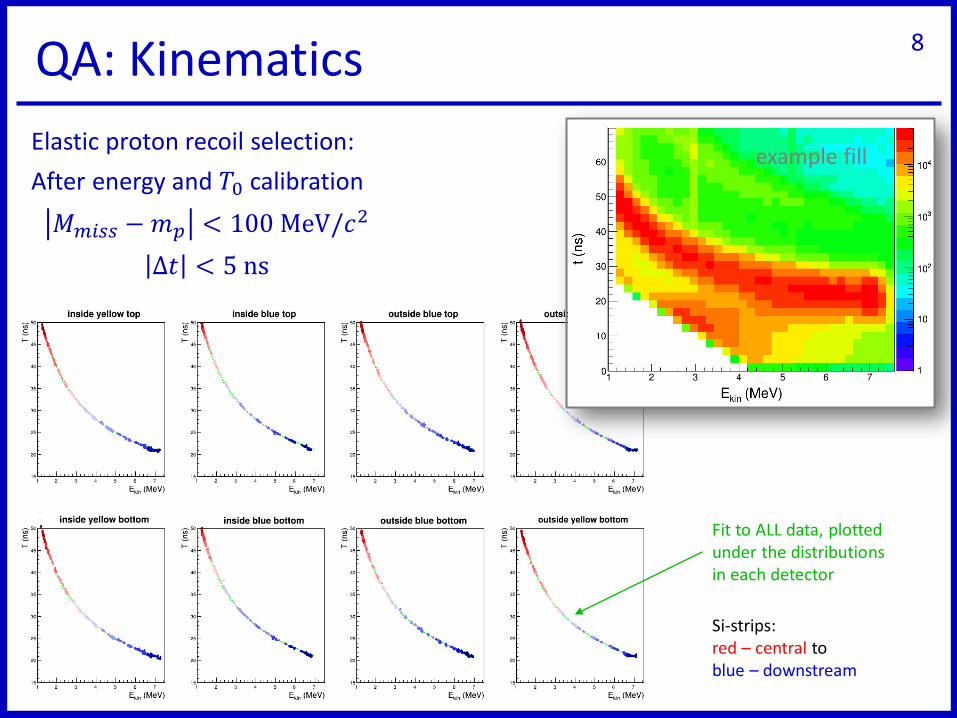
QA: Kinematics 8

Elastic proton recoil selection:

After energy and 𝑇0 calibration

𝑀𝑚𝑖𝑠𝑠 −𝑚𝑝 < 100 MeV/𝑐2

Δ𝑡 < 5 ns

Fit to ALL data, plotted under the distributions in each detector

Si-strips:red – central to blue – downstream

example fill

Detector Alignment 9

Magnetic holding field for target polarization changes acceptance of detectors on left and right sides

Outer correction field is adjusted for compensation

For missing proton mass:

sin 𝜃 =𝑝′

2 ⋅ 𝑚𝑝 ⋅ 𝑝𝐵(2 ⋅ 𝐸 + 2 ⋅ 𝑚𝑝 − 𝑇𝑅)

Compare with geometry ofdetector (averaged over 12 strips)

p+Au and p+Al operation had asignificant beam angle on thejet target

example detector

Missing mass:

𝑀𝑚𝑖𝑠𝑠2 =

𝐸 +𝑚𝑝 − 𝐸′

𝑝𝐵 − 𝑝′

2

Non-relativistic recoil:

𝑝′ = 2𝑚𝑝𝑇𝑅

swit

ch t

o p

+Au

swit

ch t

o p

+Alchange in STAR

rotators

fiel

d c

orr

ecti

on

𝑃𝐵𝑒𝑎𝑚 = −휀𝐵𝑒𝑎𝑚휀𝑇𝑎𝑟𝑔𝑒𝑡

𝑃𝑇𝑎𝑟𝑔𝑒𝑡

❶

Polarization independent background

휀 =𝑁↑−𝑁↓

𝑁↑+𝑁↓+2∙𝑁𝑏𝑔⇒

𝜀𝐵

𝜀𝑇=

𝑁𝐵↑−𝑁𝐵

↓

𝑁𝑇↑−𝑁𝑇

↓

❷

Polarization dependent background

휀 =휀𝑖𝑛𝑐 − 𝑟 ∙ 휀𝑏𝑔

1 − 𝑟background fraction 𝑟 = 𝑁𝑏𝑔/𝑁

from Breit-Rabimeasurement

Asymmetries & Polarization 10

휀 = 𝐴𝑁 ∙ 𝑃

measure

Backgro

un

d

Backgro

un

dSIG

NA

L

SIGN

AL

Inclusive

Inclusive

RHIC bunch

RHIC bunch

Signal & Background I 11

Abort gaps are not aligned at polarimeter location

Use abort gaps for background and clean signal identification

beam

beam

detecto

rd

etector

Signal & Background II 12

𝑀𝑚𝑖𝑠𝑠 −𝑀𝑝 < 50 MeV/𝑐2

𝑀𝑚𝑖𝑠𝑠 −𝑀𝑝 > 120 MeV/𝑐2

Example (logarithmic z-scale)

Δ𝑡: difference of measured time-of-flight to elastic signal, 𝑡(𝑇𝑅)

Δ𝑚𝑚𝑖𝑠𝑠: difference of missing mass to scattered proton (geometry after alignment correction)

Position of elastic proton signal is independent of energy and detector

Vertical stripes are a remnant of the spatial detector resolution

Punch through cuts are already applied

Define signal and background regions by missing mass

Signal & Background III 13

inclusive (normalized to peak)

𝑀𝑚𝑖𝑠𝑠 −𝑚𝑝 < 50 MeV/𝑐2

background (normalized to signal at 18 < Δ𝑡 < 25 ns)

𝑀𝑚𝑖𝑠𝑠 −𝑚𝑝 > 120 MeV/𝑐2

background fraction

Example (blue beam, 2 < 𝐸𝑘𝑖𝑛 < 3 MeV)

o Background in yellow abort gap (should be clean blue signal)

o Signal in blue abort gap (should be only background from yellow beam)

The normalization is same as above → only for comparison of shape and source of background

normalization

well described by normalization at 18 < Δ𝑡 < 25 ns

Background Sources 14

Example (blue beam, 3 < 𝐸𝑘𝑖𝑛 < 4 MeV) From 𝑝 + 𝐴𝑢 operation

Typical bunch shape of Au-beam seen in full background, dominates earlybackground

Late background mainly from signal beam

Using signal cuts in blue abort gap:

𝑀𝑚𝑖𝑠𝑠 −𝑚𝑝 < 50 MeV/𝑐2

Fill-by-fill background fraction depends on conditions of both beams → important for beam polarization measurement

still excellent agreementBackground fraction 𝑟 = 𝑁𝑏𝑔/𝑁

Asymmetry Examples 15

From Ԧ𝑝 + 𝐴𝑢 operation

Blue beam (proton on jet target)

Clear asymmetry within Δ𝑡 = ± 5 ns

Background asymmetry consistent with zero

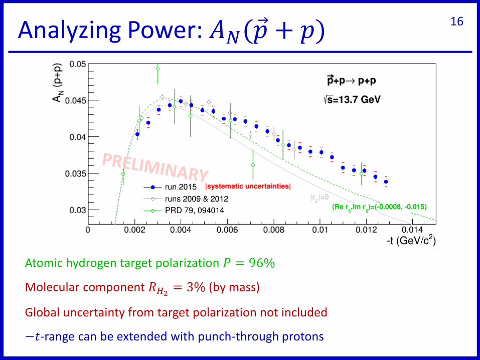
Analyzing Power: 𝐴𝑁( Ԧ𝑝 + 𝑝) 16

Atomic hydrogen target polarization 𝑃 = 96%

Molecular component 𝑅𝐻2 = 3% (by mass)

Global uncertainty from target polarization not included

−𝑡-range can be extended with punch-through protons

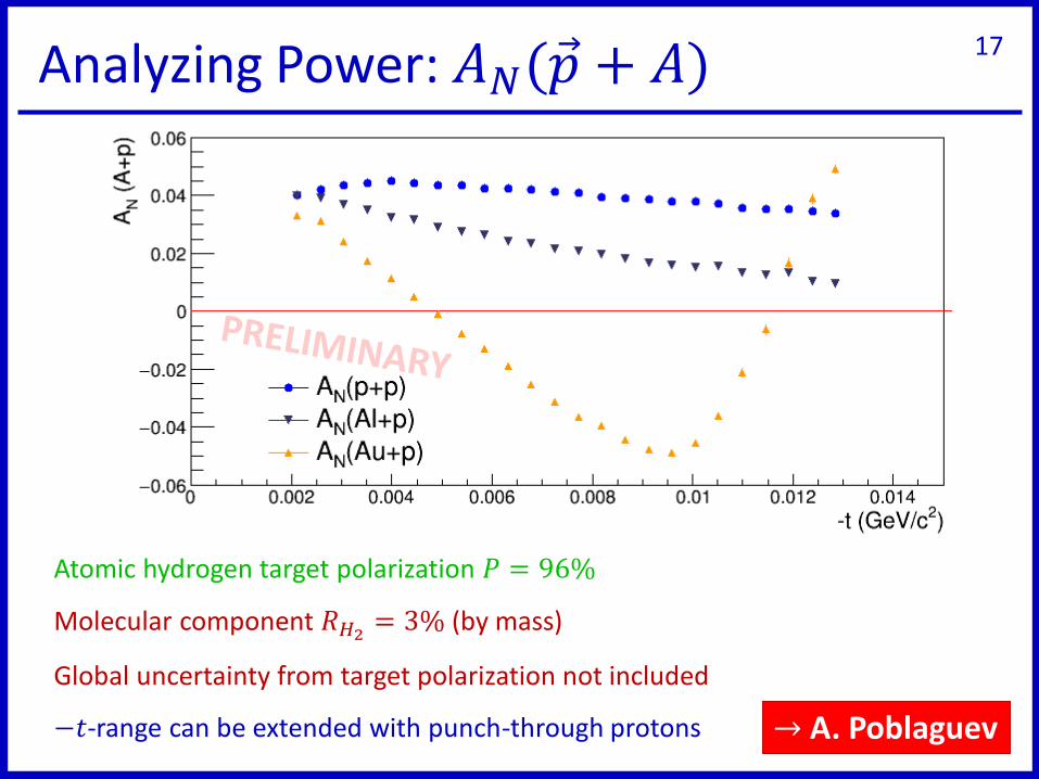
Analyzing Power: 𝐴𝑁( Ԧ𝑝 + 𝐴) 17

Atomic hydrogen target polarization 𝑃 = 96%

Molecular component 𝑅𝐻2 = 3% (by mass)

Global uncertainty from target polarization not included

−𝑡-range can be extended with punch-through protons → A. Poblaguev

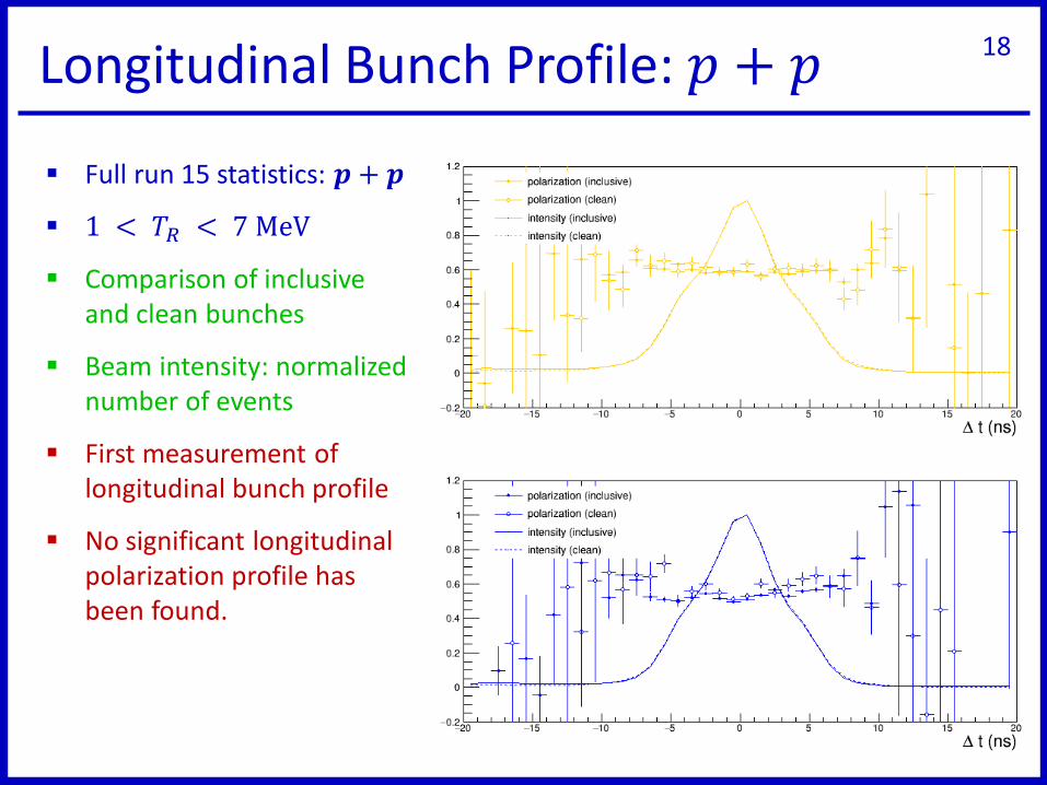
Longitudinal Bunch Profile: 𝑝 + 𝑝 18

Full run 15 statistics: 𝒑 + 𝒑

1 < 𝑇𝑅 < 7 MeV

Comparison of inclusive and clean bunches

Beam intensity: normalized number of events

First measurement of longitudinal bunch profile

No significant longitudinal polarization profile has been found.

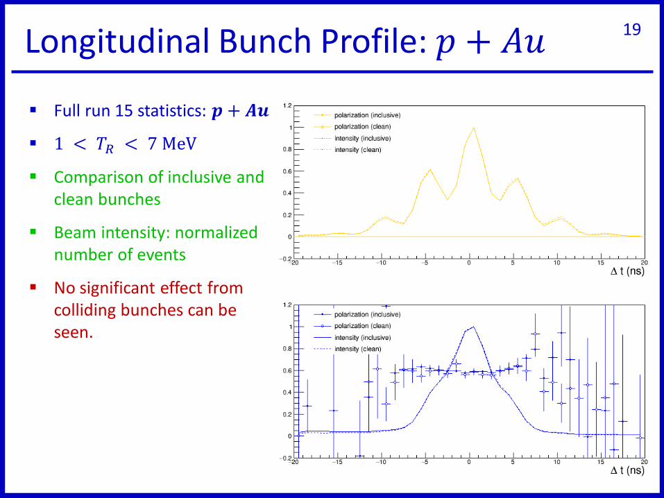
Longitudinal Bunch Profile: 𝑝 + 𝐴𝑢 19

Full run 15 statistics: 𝒑 + 𝑨𝒖

1 < 𝑇𝑅 < 7 MeV

Comparison of inclusive and clean bunches

Beam intensity: normalized number of events

No significant effect from colliding bunches can be seen.

Final Beam Polarizations 20

Atomic hydrogen target polarization 96%𝐻2 content 3% (mass)

Ratio of target/beam asymmetries1 < 𝐸𝑟𝑒𝑐𝑜𝑖𝑙 < 7 MeV (six bins)

Fit to constant

use fixed 𝐴𝑁 for 𝑝 + 𝑝 use fill by fill ratio for 𝑝 + 𝐴

Luminosity Weighted Polarization 21

𝑃 =∫ 𝑃 𝑥, 𝑦, 𝑡 ⋅ 𝐼 𝑥, 𝑦, 𝑡 𝑑𝑥𝑑𝑦𝑑𝑡

∫ 𝐼 𝑥, 𝑦, 𝑡 𝑑𝑥𝑑𝑦𝑑𝑡

Experiments

HJET Polarimeter

Carbon Polarimeter

𝑃 =∫ 𝑃 𝑥, 𝑦, 𝑡 ⋅ 𝐼𝐵 𝑥, 𝑦, 𝑡 ⋅ 𝐼𝑌 𝑥, 𝑦, 𝑡 𝑑𝑥𝑑𝑦𝑑𝑡

∫ 𝐼𝐵 𝑥, 𝑦, 𝑡 ⋅ 𝐼𝑌 𝑥, 𝑦, 𝑡 𝑑𝑥𝑑𝑦𝑑𝑡

sweep

beam width

𝑃 = 𝑃𝑚𝑎𝑥 ⋅𝐼

𝐼𝑚𝑎𝑥

𝑅

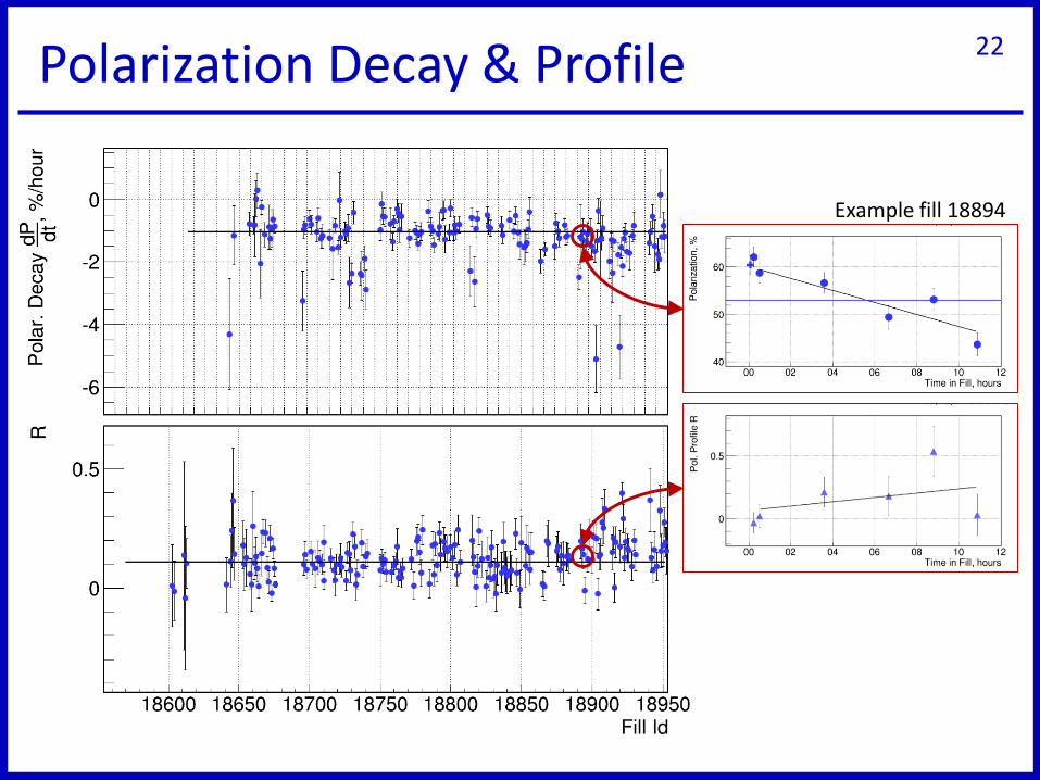
Polarization Decay & Profile 22

Example fill 18894

o Polarimetry at RHIC

• Essential input for experiments

• Fast feedback during collider operation

Fast polarization measurement with Carbon targets

• Polarization decay and transverse profile

Absolute normalization with polarized hydrogen jet target

o Analyzing power with new detectors in 2015 → improved precision and systematic studies

o New asymmetries from elastic proton-heavy-ion scattering

o Longitudinal polarization profile

o Final beam polarizations are fully background corrected

Summary 23

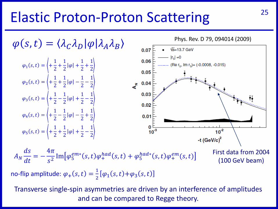
𝜑 𝑠, 𝑡 = 𝜆𝐶𝜆𝐷 𝜑 𝜆𝐴𝜆𝐵Phys. Rev. D 79, 094014 (2009)

𝜑1 𝑠, 𝑡 = +1

2+1

2𝜑 +

1

2+1

2

𝜑2 𝑠, 𝑡 = +1

2+1

2𝜑 −

1

2−1

2

𝜑3 𝑠, 𝑡 = +1

2−1

2𝜑 +

1

2−1

2

𝜑4 𝑠, 𝑡 = +1

2−1

2𝜑 −

1

2+1

2

𝜑5 𝑠, 𝑡 = +1

2+1

2𝜑 +

1

2−1

2

𝐴𝑁𝑑𝑠

𝑑𝑡= −

4𝜋

𝑠2Im 𝜑5

𝑒𝑚∗ 𝑠, 𝑡 𝜑+ℎ𝑎𝑑 𝑠, 𝑡 + 𝜑5

ℎ𝑎𝑑∗ 𝑠, 𝑡 𝜑+𝑒𝑚(𝑠, 𝑡)

no-flip amplitude: 𝜑+ 𝑠, 𝑡 =1

2𝜑1 𝑠, 𝑡 +𝜑3 𝑠, 𝑡

First data from 2004 (100 GeV beam)

Elastic Proton-Proton Scattering 25

Transverse single-spin asymmetries are driven by an interference of amplitudes and can be compared to Regge theory.

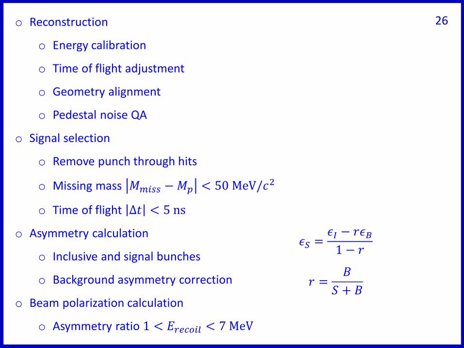
26o Reconstruction

o Energy calibration

o Time of flight adjustment

o Geometry alignment

o Pedestal noise QA

o Signal selection

o Remove punch through hits

o Missing mass 𝑀𝑚𝑖𝑠𝑠 −𝑀𝑝 < 50 MeV/𝑐2

o Time of flight Δ𝑡 < 5 ns

o Asymmetry calculation

o Inclusive and signal bunches

o Background asymmetry correction

o Beam polarization calculation

o Asymmetry ratio 1 < 𝐸𝑟𝑒𝑐𝑜𝑖𝑙 < 7MeV

𝜖𝑆 =𝜖𝐼 − 𝑟𝜖𝐵1 − 𝑟

𝑟 =𝐵

𝑆 + 𝐵

Energy Calibration 27

Calibrations are done every few days:

o Gain

o Entrance window (dead layer)

Two different α-sources

𝐸𝛼 𝐺𝑑 = 3.183 MeV

𝐸𝛼 𝐴𝑚 = 5.486 MeV

Resolution of peak finding is within 1 ADC count

Stopping power for protons and𝛼-particles from NIST database:

∆𝐸𝛼(𝐴𝑚) = 0.72 ∙ ∆𝐸𝛼 𝐺𝑑

∆𝐸𝑃 = 0.44 ∙ ∆𝐸𝛼(𝐺𝑑) ∙ 𝐸[𝑀𝑒𝑉]−0.64

example

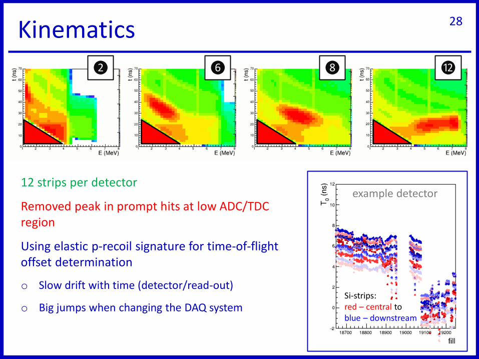
Kinematics 28

❷ ❻ ❽ ⓬

12 strips per detector

Removed peak in prompt hits at low ADC/TDC region

Using elastic p-recoil signature for time-of-flight offset determination

o Slow drift with time (detector/read-out)

o Big jumps when changing the DAQ system

example detector

Si-strips:red – central to blue – downstream

Stopped Recoil Protons 29

Slope of rise in waveform can be used to identify punch-through particles

Normalized waveform rise (4.5 < 𝐸 < 5.5 MeV)in each detector

Independent of DAQ system (CAMAC/VME)

Remove punch-through particles:

𝑇𝑘𝑖𝑛 (MeV)

𝛿 𝐴𝐷𝐶(a.u.)

example detector

(δADC < −0.5) ∧ (𝛿𝐴𝐷𝐶 < 8.5 − 1.5 ∗ 𝑇𝑘𝑖𝑛)

Normalized to 𝐴𝐷𝐶max

Slope 𝛿𝐴𝐷𝐶 calculated in six 𝑇𝐷𝐶 binsaround ½ 𝐴𝐷𝐶max

Ԧ𝑝+𝑝

, yel

low

bea

m

Ԧ𝑝+𝑝

, blu

e b

eam

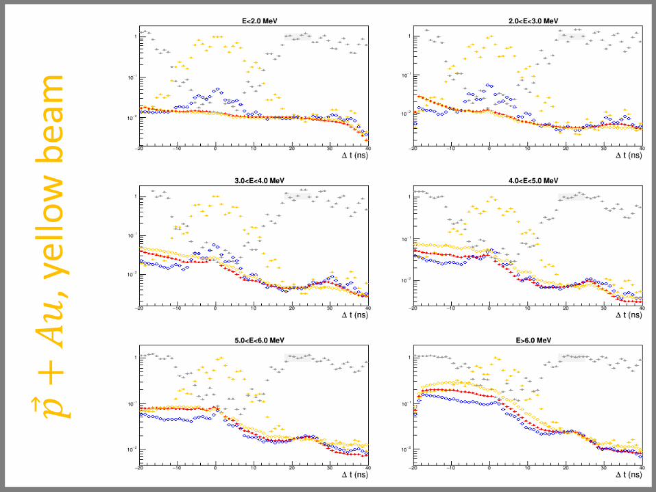
Ԧ𝑝+𝐴𝑢

, yel

low

bea

m

Ԧ𝑝+𝐴𝑢

, blu

e b

eam

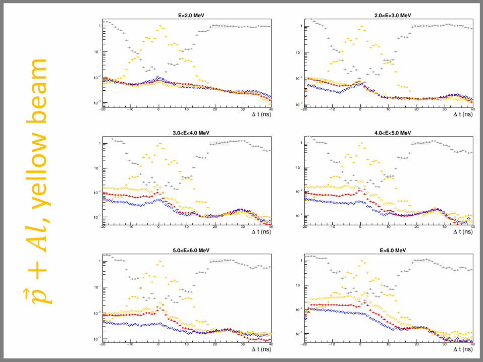
Ԧ𝑝+𝐴𝑙,

yel

low

bea

m

Ԧ𝑝+𝐴𝑙,

blu

e b

eam

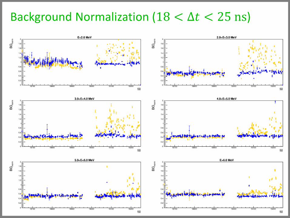
Background Normalization (18 < Δ𝑡 < 25 ns)

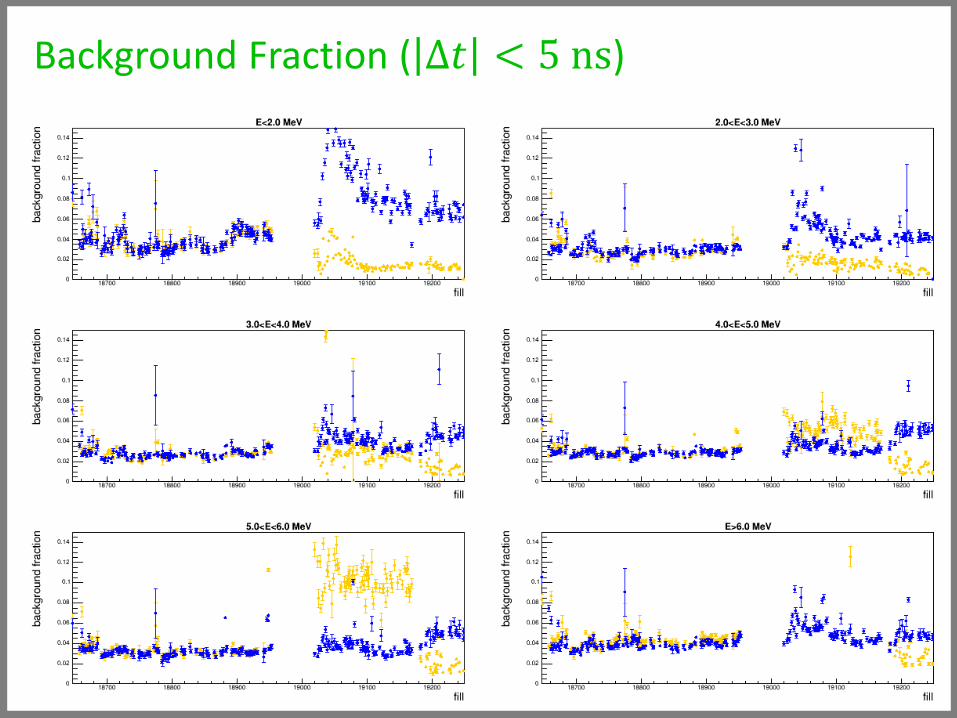
Background Fraction ( Δ𝑡 < 5 ns)

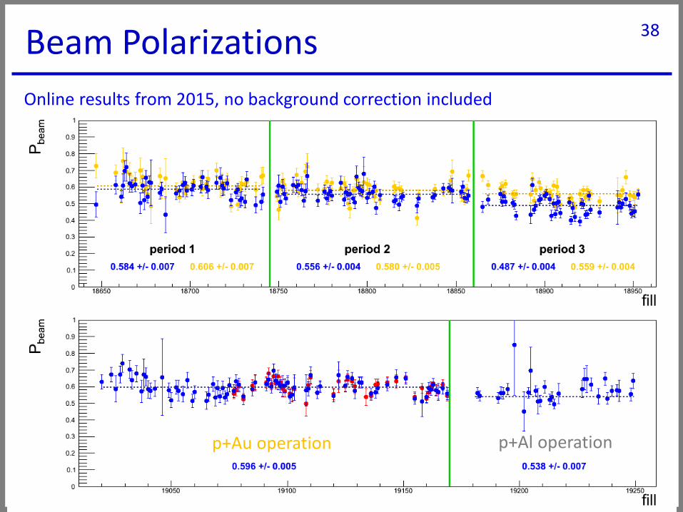
Beam Polarizations 38

Online results from 2015, no background correction included

p+Au operation p+Al operation

𝐴𝑁 in Elastic Ԧ𝑝 + 𝑝 Scattering 39

Noise threshold cut: 0.20 for 𝑝 + 𝑝, 0.15 for 𝑝 + 𝐴

p+A may still have some issues with high background fractions and changing beam conditions

40Summary p+AlBeam polarizations

Full run 15 statistics, p+Al

Comparison of inclusive and clean bunches

41Pedestal Noisefill 18677

channel 64(with CAMAC)

fill 19214channel 81(with VME)

𝑃𝑗𝑒𝑡↑

𝑃𝑗𝑒𝑡↓

solid/dashed: 𝑃𝑏𝑒𝑎𝑚↑ /𝑃𝑏𝑒𝑎𝑚

↓

The noise is mainly on one side of the detector (outside).

It changes the waveform quality (slope) for low energies and leads to asymmetric loss of events.

𝑟𝑚𝑠𝑝𝑒𝑑↑ − 𝑟𝑚𝑠𝑝𝑒𝑑

↓

(*) can use a fit for VME data, but resolution of CAMAC is too small

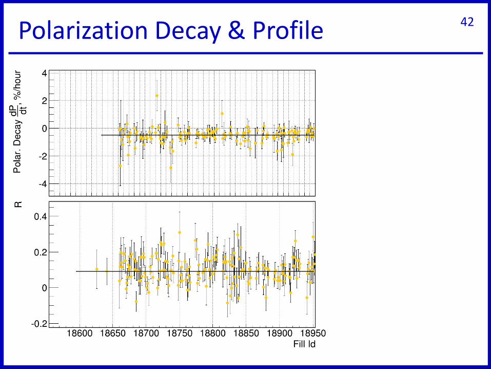
Polarization Decay & Profile 42