"/ think and think for months and years. Ninety-nine times, the conclusion is false. The hundredth time I am right." Albert Einstein.

Welcome message from author
This document is posted to help you gain knowledge. Please leave a comment to let me know what you think about it! Share it to your friends and learn new things together.
Transcript
"/ think and think for months and years. Ninety-nine times, the conclusion is false. The hundredth time I am right."
Albert Einstein.

University of Alberta
PLANT PROTEIN LOCALIZATION BASED ON FREQUENT DISCRIMINATIVE
SUBSEQUENCES AND PARTITION-BASED SUBSEQUENCES
by
Seyed-Vahid Jazayeri
A thesis submitted to the Faculty of Graduate Studies and Research in partial fulfillment of the requirements for the degree of Master of Science.
Department of Computing Science
Edmonton, Alberta Fall 2008

1*1 Library and Archives Canada
Published Heritage Branch
395 Wellington Street Ottawa ON K1A0N4 Canada
Bibliotheque et Archives Canada
Direction du Patrimoine de I'edition
395, rue Wellington Ottawa ON K1A0N4 Canada
Your file Votre reference ISBN: 978-0-494-47270-5 Our file Notre reference ISBN: 978-0-494-47270-5
NOTICE: The author has granted a nonexclusive license allowing Library and Archives Canada to reproduce, publish, archive, preserve, conserve, communicate to the public by telecommunication or on the Internet, loan, distribute and sell theses worldwide, for commercial or noncommercial purposes, in microform, paper, electronic and/or any other formats.
AVIS: L'auteur a accorde une licence non exclusive permettant a la Bibliotheque et Archives Canada de reproduire, publier, archiver, sauvegarder, conserver, transmettre au public par telecommunication ou par I'lnternet, prefer, distribuer et vendre des theses partout dans le monde, a des fins commerciales ou autres, sur support microforme, papier, electronique et/ou autres formats.
The author retains copyright ownership and moral rights in this thesis. Neither the thesis nor substantial extracts from it may be printed or otherwise reproduced without the author's permission.
L'auteur conserve la propriete du droit d'auteur et des droits moraux qui protege cette these. Ni la these ni des extraits substantiels de celle-ci ne doivent etre imprimes ou autrement reproduits sans son autorisation.
In compliance with the Canadian Privacy Act some supporting forms may have been removed from this thesis.
While these forms may be included in the document page count, their removal does not represent any loss of content from the thesis.
•*•
Canada
Conformement a la loi canadienne sur la protection de la vie privee, quelques formulaires secondaires ont ete enleves de cette these.
Bien que ces formulaires aient inclus dans la pagination, il n'y aura aucun contenu manquant.

To my respected parents, my nice grandmother and my lovely wife, Mojdeh.
Abstract
Proteins, important macromolecules in living cells, are present in different loca
tions within the cells, and a few are transported to the extracellular space. Each
protein has a distinct function, and to fulfill that function they must be localized to
the correct position in the cell. Therefore, discovering the localization of a protein
helps analyze its role in the living cell. Extracellular proteins are of high importance
due to their responsibility for vital functions such as nutrition acquisition, protec
tion from pathogens, etc. Hence, characterizing these proteins and distinguishing
them from intracellular proteins is of high interest to biologists. Nonetheless, this
problem is very challenging because of the small number of available extracellular
proteins1.
This work focuses on extracellular and intracellular localizations. Using asso
ciative classifier we acquire a set of accurate, small and interpretable localization
rules that can be used for further biological analysis. To classify proteins, which are
linear sequences of amino acids, one should represent these by a set of features. In
this work, the most frequent discriminative subsequences as well as partition-based
subsequences are studied, i.e.,subsequences frequent in some partitions along pro
tein sequences. The achievement of high F-Measure for predicting extracellular
proteins shows high discrimination ability of the selected features.
Our dataset contains only 127 extracellular proteins
Acknowledgements
During my study at the University of Alberta, I was very fortunate to be with a
number of people who helped me grow not only academically, but also in many
aspects of my life. Here is a chance for me to thank them all for their support,
guidance and friendship. Without their companionship, I might not have advanced
this far.
My deepest appreciation is dedicated to my parents and my lovely grandmother
for their endless and unconditional support and love. After all my formal education,
I should say that they have been the kindest and greatest teachers ever in my life
who taught me most. Whatever success I achieve, it would have never been possible
without their encouragement and consideration in the early stages of my life. Words
can never express how grateful I am to them. May dedicating this thesis to them
make up a little for what they have done so far for me. I should also offer a bunch
of thanks to my unexampled sister and brothers, and my dear siblings-in-law who
have been always supportive to me
Special thanks to my supervisor, Dr. Osmar R. Zaiane, for his unsparing guid
ance, supervision, and helps. He taught me how to think wide, to challenge diffi
culties without any frustration and to wait for a future success. His kindness toward
me and my wife, another student of his, is admired for ever.
My sincere gratitude goes to my examiners, Dr. Randy Goebel and Warren J.
Gallin who took their valuable time to carefully review my thesis, and provided
me with constructive comments and directions to improve the quality of this dis
sertation. Also thanks to Yang Wang for his well documented M.Sc. thesis. His
dissertation helped me a lot to acquire background knowledge on what I did in
my project. I am grateful to all the authors who shared their data and codes, and
generally all who contributed to the fulfillment of my thesis.
Appreciations to Dr. Davood Rafiei who nominated and helped me to be granted
the computing science entrance scholarship. It had a considerable influence on my
success in the early months of my arrival to Canada.
It was a great pleasure for me to be a member of the Database Research Group.
I wish to thank the professors and other fellow students, Reza Sherkat, Pirooz
Chubak, Reza Sa'do-din, Pouria Pirzadeh, Gabriella Moise, Luiza Antonie, Baljeet
Malhotra and Amit Satsangi. They made the database Lab a pleasant environment
to work in for long hours without feeling tired.
My friends in Edmonton made a big difference in my life here. Being with them
was enough to make good memories and stop thinking about the hardship of being
miles away from family. Having them makes Edmonton with tiresome and durable
cold winters, an Edmonton which is a nice place to live. There is not enough space
to thank them all. However, I should specially mention Mehdi and Parisa, Ali Gorji,
Ali Azad, Mohsen Niksiar, Banafsheh and Lise Menard.
And after all, my most special thanks go to my lovely wife, Mojdeh. I may
never forget her unlimited support and love along the late nights she stayed with
me awake, even in the Database Lab on weekends, with no reason other than only
accompanying me in the difficulties of my project. She was someone who most
times discovered the errors and problems of my computer programs whenever I
was frustrated of resolving them. The success of my thesis project partly owes her
support. I am cordially thankful to her.
Contents
1 Introduction 1 1.1 Background, Problem Definition and Approach 1 1.2 Dissertation Organization 6
2 Related Work 7 2.1 Work Related to Protein Subcellular Localization 7
2.1.1 Prediction Based on N-Terminal Sorting Signals 7 2.1.2 Prediction Based on Protein Annotations 9 2.1.3 Prediction Based on Amino Acid Composition 10 2.1.4 Prediction Based on Frequent Subsequences 11 2.1.5 Prediction Based on Integrative Approaches 12 2.1.6 Challenges and Limitations of the State-of-the-Art
Methods 12 2.2 Work Related to Frequent Subsequence Mining 14
3 Protein Feature Extraction 18 3.1 History of Frequent-Subsequence-Based Feature Mining Algorithms 19
3.1.1 Class-Specific Subsequence Mining 21 3.1.2 M-Most Frequent Subsequences 21 3.1.3 M-Most Frequent Maximal Subsequences 22 3.1.4 N-Most Discriminative Motifs 23 3.1.5 N-Most Discriminative Motifs Based on IC Localizations . 23 3.1.6 Dynamic Support-Feature Minimization 24 3.1.7 Dynamic Support-Rare Motif Detection 27 3.1.8 Dynamic Support - Most Discriminative Frequent Motif . . 28 3.1.9 N-Best (Longest) Motifs 28
3.2 Discriminative and Frequent Partition-Based Subsequences 31
4 Associative Classification for Protein Localization 37 4.1 Building Associative Rule Classifier (Training Phase) 38
4.1.1 Mining Frequent Itemsets 39 4.1.2 Abridging Itemsets 40 4.1.3 Computing the Confidence of a Rule 43 4.1.4 Pruning the Rules 44
4.2 Evaluating Associative Rule Classifier (Testing Phase) 46
5 Experimental Results 49 5.1 Dataset and Evaluation Methodology 49 5.2 Mining Frequent Partition-Based Subsequences 50 5.3 Classification Algorithms and the Prediction Model Evaluation . . . 53
5.3.1 INN Classifier 54 5.3.2 Associative Classifier 54
5.3.3 SVM Classifier 55 5.3.4 Decision Tree 56 5.3.5 Combination of Associative and INN Classifiers 57 5.3.6 Combination of SVM and INN Classifiers 59 5.3.7 Combination of Decision Tree and INN Classifiers 60 5.3.8 Comparison of Different Classifiers 60
5.4 The Reliability of the Parameter Setting Approach For Feature Mining 61
6 Conclusion And Future Work 65
Bibliography 67
List of Tables
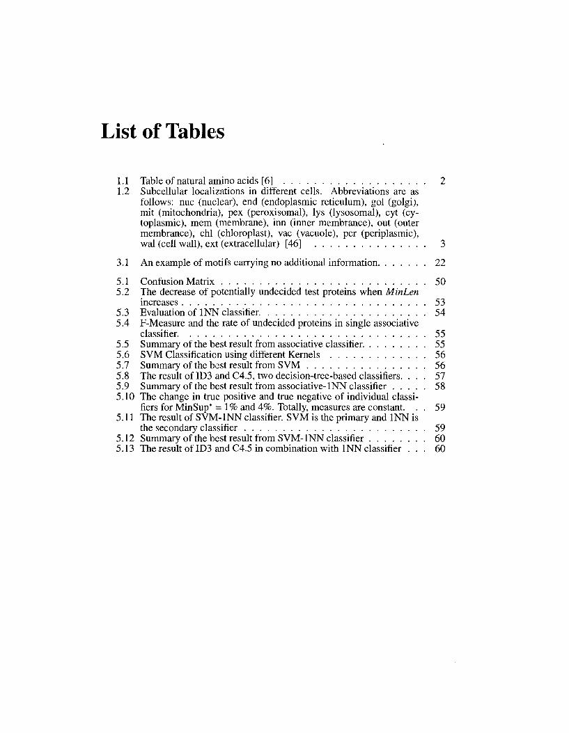
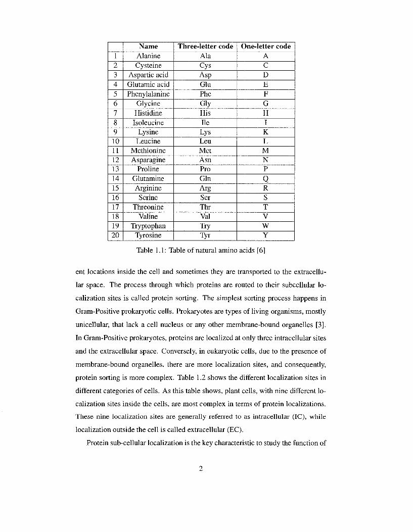
1.1 Table of natural amino acids [6] 2 1.2 Subcellular localizations in different cells. Abbreviations are as
follows: nuc (nuclear), end (endoplasmic reticulum), gol (golgi), mit (mitochondria), pex (peroxisomal), lys (lysosomal), cyt (cytoplasmic), mem (membrane), inn (inner membrance), out (outer membrance), chl (chloroplast), vac (vacuole), per (periplasmic), wal (cell wall), ext (extracellular) [46] 3
3.1 An example of motifs carrying no additional information 22
5.1 Confusion Matrix 50 5.2 The decrease of potentially undecided test proteins when MinLen
increases 53 5.3 Evaluation of INN classifier 54 5.4 F-Measure and the rate of undecided proteins in single associative
classifier. 55 5.5 Summary of the best result from associative classifier. 55 5.6 SVM Classification using different Kernels 56 5.7 Summary of the best result from SVM 56 5.8 The result of ID3 and C4.5, two decision-tree-based classifiers. . . . 57 5.9 Summary of the best result from associative-INN classifier 58 5.10 The change in true positive and true negative of individual classi
fiers for MinSup* = 1% and 4%. Totally, measures are constant. . . 59 5.11 The result of SVM-INN classifier. SVM is the primary and INN is
the secondary classifier 59 5.12 Summary of the best result from SVM-INN classifier 60 5.13 The result of ID3 and C4.5 in combination with INN classifier . . . 60
List of Figures
1.1 Structure of Protein [ 1 ]. The locations that may interact due to their close distance are circled 4
1.2 Real examples of the human readable rules that our associative classifier discovered from the data 5
2.1 Histogram representation of the amino acid composition of an extracellular protein 11
2.2 A naive algorithm for mining frequent subsequences 15 2.3 An example of candidate generation. 5 i and 52, two frequent sub
sequences of length 5, generate 53, a candidate subsequence of length 6 16
2.4 The GST of three strings: 1) JKLMK, 2) JKDL, 3)MEJK 17
3.1 The length of proteins in the feature dataset where MinSup is appropriate enough for all proteins to be expressed by at least one motif 24
3.2 The effect of minimum support on the number of mined long motifs and silent proteins in EC and IC classes 25
3.3 Dividing the virtual protein CDEFGHKLMNPQ into 2 and 4 parts and the address of each partition. Trivially location 1/2 and 2/4 are not the same; Neither are 2/2 and 4/4 32
3.4 Partition-Frequency table of a subsequence 5 where partitioning proteins to 1, 2, and 3 is investigated (MaxPart - 3) 33
3.5 Illustration of Equation 3.2 33
4.1 The histogram of the length of transactions in our best feature dataset on which we coud make the most accurat classifier 39
4.2 Two layouts of storing transactions. The bitmap vertical layout is used in Eclat 40
4.3 The Trie representation of IC protein transactions 44 4.4 An example of a test protein and the localization rules matching the
protein 47 4.5 Two similar extracellular proteins that are mutated from a same se
quence 48
5.1 The influence of MinS up on the number of silent proteins of test data 52 5.2 Average length of subsequences for different MinS up values where
MinLen = 3 52 5.3 5.3(a) The F-Measure of the combined model of associative and
INN classifiers, and 5.3(b) The portion of undecided proteins that are localized by INN classifier 58
5.4 The comparison of different models in terms of their prediction accuracy 61
5.5 With MinSup fixed to 0.2%, initial value 7 for MinLen has been the best setting 62
5.6 With MinLen fixed to 7, initial value 0.2% for MinSup has been the best setting 62
5.7 The increase of F-Measure in associative classifier by partitioning proteins 64
5.8 The increase of F-Measure in associative-INN classifier by partitioning proteins 64
Chapter 1
Introduction
Proteins are one of the main structures of living cells that conduct different pro
cesses and functions in the cell. Proteins, at the simplest representation, are lin
ear sequences of amino acids, and so far twenty standard amino acids have been
identified in proteins.1. These amino acids are coded by twenty alphabetic char
acters as shown in Table 1.1. Therefore, proteins can be considered as character
strings of different length varying from 41 amino acids or less, for a mitochondrial
plant protein, to 3,705 or more, for an outer membrane plant protein. Biological
experiments indicate that amino acid sequences encode information about protein
structures, functions, localizations, etc .
Through genome sequencing projects, many datasets of raw biological sequences
are collected, and are publicly available for researchers. With the interest to study
genome sequences and the rapid growth of collected biological data, which adds
complexity to the study and analysis of the sequences, there is a tendency toward
utilizing computational algorithms and tools. This research addresses some algo
rithms to challenge one of the important problems about plant protein localizations.
1.1 Background, Problem Definition and Approach
One of the important problems in the biology community is the functional clas
sification of proteins based on their structures, localizations, or other properties.
In order for proteins to accomplish a specific function, they concentrate in differ-
1 Unlike other amino acids that are present in biological proteins, Selenocysteine, the 21st amino acid, is inserted at a UGA codon in the context of other sequences within the mRNA.
1
1 2 3 4 5 6 7 8 9 10 11 12 13 14 15 16 17 18 19 20
Name Alanine Cysteine
Aspartic acid Glutamic acid Phenylalanine
Glycine Histidine Isoleucine
Lysine Leucine
Methionine Asparagine
Proline Glutamine Arginine
Serine Threonine
Valine Tryptophan
Tyrosine
Three-letter code Ala Cys Asp Glu Phe Gly His He Lys Leu Met Asn Pro Gin Arg Ser Thr Val Try Tyr
One-letter code A C D E F G H I K L M N P
Q R S T V W Y
Table 1.1: Table of natural amino acids [6]
ent locations inside the cell and sometimes they are transported to the extracellu
lar space. The process through which proteins are routed to their subcellular lo
calization sites is called protein sorting. The simplest sorting process happens in
Gram-Positive prokaryotic cells. Prokaryotes are types of living organisms, mostly
unicellular, that lack a cell nucleus or any other membrane-bound organelles [3].
In Gram-Positive prokaryotes, proteins are localized at only three intracellular sites
and the extracellular space. Conversely, in eukaryotic cells, due to the presence of
membrane-bound organelles, there are more localization sites, and consequently,
protein sorting is more complex. Table 1.2 shows the different localization sites in
different categories of cells. As this table shows, plant cells, with nine different lo
calization sites inside the cells, are most complex in terms of protein localizations.
These nine localization sites are generally referred to as intracellular (IC), while
localization outside the cell is called extracellular (EC).
Protein sub-cellular localization is the key characteristic to study the function of
2
Category Animal Plant Fungi
Gram-Positive bacteria Gram-Negative bacteria
Subcellular Localizations nuc, end, gol, mit, pex, lys, cyt, mem, ext nuc, end, gol, mit, pex, chl, vac, cyt, mem, ext nuc, end, gol, mit, pex, vac, cyt, mem, ext cyt, wal, mem, ext cyt, inn, per, wal, out, ext
Table 1.2: Subcellular localizations in different cells. Abbreviations are as follows: nuc (nuclear), end (endoplasmic reticulum), gol (golgi), mit (mitochondria), pex (peroxisomal), lys (lysosomal), cyt (cytoplasmic), mem (membrane), inn (inner membrance), out (outer membrance), chl (chloroplast), vac (vacuole), per (periplas-mic), wal (cell wall), ext (extracellular) [46]
proteins. In plants, EC proteins are responsible for vital functions such as "nutrition
acquisition, communication with other soil organisms, protection from pathogens,
and resistance to disease and toxic metals" [48]. Therefore, they are of high impor
tance for the cells and are a target of analysis in the biology community. Herein,
we particularly focus on characterizing and predicting EC proteins by learning and
classifying proteins to EC or IC locations.
Localization of proteins has been a research interest for bio-informaticians and
machine learners for some time, but it is still a challenging problem mainly due to
the lack of training data, and when data exists, to severe imbalance in the training
data. Another difficulty is the identification of appropriate features in the data to
accurately localize proteins. Some have used simple distribution of amino acids
(i.e.,protein composition), subsequences, special signatures or combinations. In
this research we start with studying frequent subsequences of proteins. The process
of localization utilizes small subsequences of the protein to direct the protein to dif
ferent localizations. Therefore, frequent subsequences, identified by our approach,
might be of direct mechanistic significance. Based on frequent subsequences, we
gradually evolve our feature mining algorithm by resolving the experimentally ob
served deficiencies of the older algorithms. Finally, we introduce the idea of taking
advantage of partitioning sequences of amino acids and identifying the relevant
partitions where some subsequences occur. These partitions appear to have dis
criminative power with regard to localization of proteins.
To do so, we transform the proteins that are originally represented as strings of
3
i f Primary protein structure u is sequence of a chain of amino acids
Amino Acids
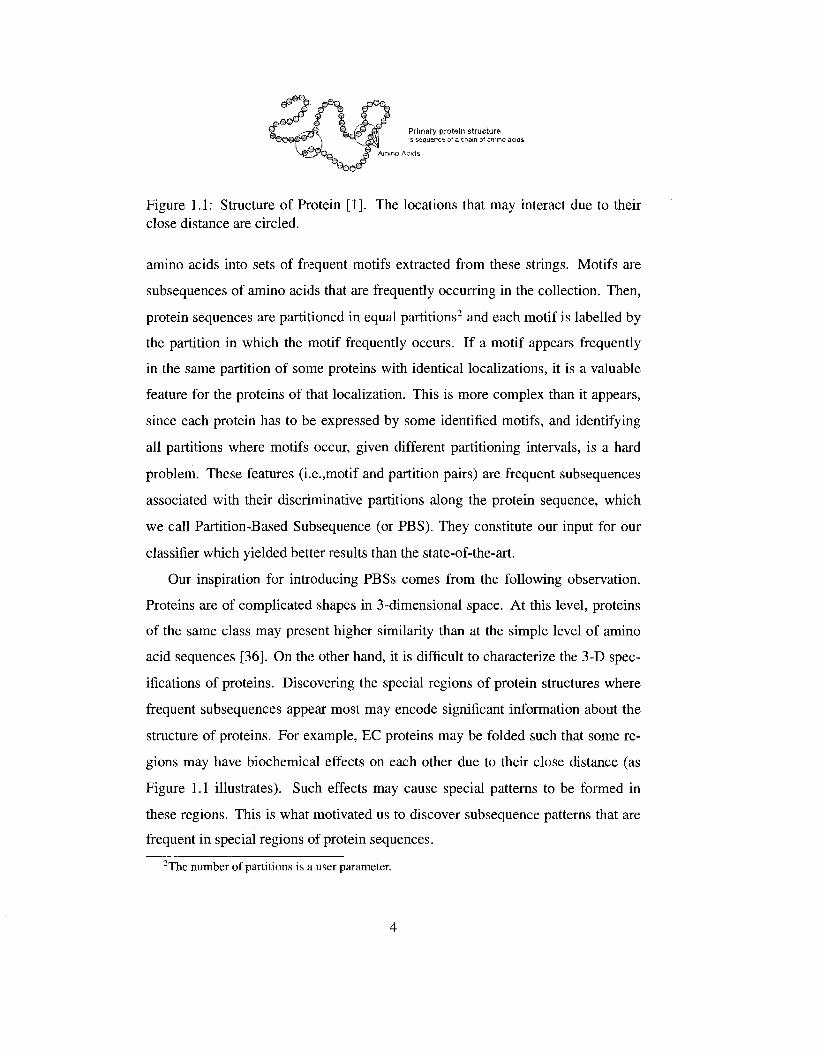
Figure 1.1: Structure of Protein [1]. The locations that may interact due to their close distance are circled.
amino acids into sets of frequent motifs extracted from these strings. Motifs are
subsequences of amino acids that are frequently occurring in the collection. Then,
protein sequences are partitioned in equal partitions2 and each motif is labelled by
the partition in which the motif frequently occurs. If a motif appears frequently
in the same partition of some proteins with identical localizations, it is a valuable
feature for the proteins of that localization. This is more complex than it appears,
since each protein has to be expressed by some identified motifs, and identifying
all partitions where motifs occur, given different partitioning intervals, is a hard
problem. These features (i.e.,motif and partition pairs) are frequent subsequences
associated with their discriminative partitions along the protein sequence, which
we call Partition-Based Subsequence (or PBS). They constitute our input for our
classifier which yielded better results than the state-of-the-art.
Our inspiration for introducing PBSs comes from the following observation.
Proteins are of complicated shapes in 3-dimensional space. At this level, proteins
of the same class may present higher similarity than at the simple level of amino
acid sequences [36]. On the other hand, it is difficult to characterize the 3-D spec
ifications of proteins. Discovering the special regions of protein structures where
frequent subsequences appear most may encode significant information about the
structure of proteins. For example, EC proteins may be folded such that some re
gions may have biochemical effects on each other due to their close distance (as
Figure 1.1 illustrates). Such effects may cause special patterns to be formed in
these regions. This is what motivated us to discover subsequence patterns that are
frequent in special regions of protein sequences.
2The number of partitions is a user parameter.
4
Other than introducing PBS, a novel type of protein features, the prediction of
EC proteins based these features is another contribution of this work. We use an
associative classifier to predict EC proteins. The reason for our choice is that asso
ciative classifiers construct an interpretable rule-based model that can be used for
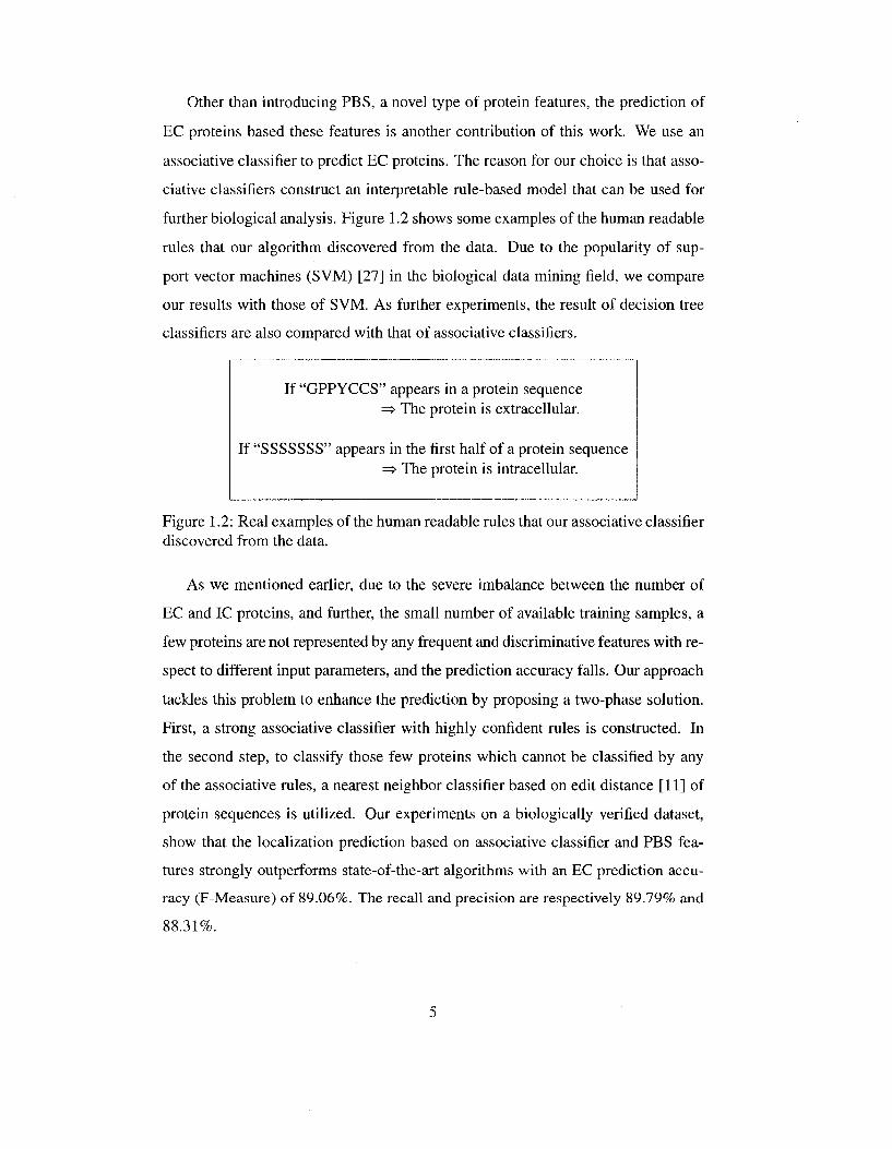
further biological analysis. Figure 1.2 shows some examples of the human readable
rules that our algorithm discovered from the data. Due to the popularity of sup
port vector machines (SVM) [27] in the biological data mining field, we compare
our results with those of SVM. As further experiments, the result of decision tree
classifiers are also compared with that of associative classifiers.
If "GPPYCCS" appears in a protein sequence => The protein is extracellular.
If "SSSSSSS" appears in the first half of a protein sequence => The protein is intracellular.
Figure 1.2: Real examples of the human readable rules that our associative classifier discovered from the data.
As we mentioned earlier, due to the severe imbalance between the number of
EC and IC proteins, and further, the small number of available training samples, a
few proteins are not represented by any frequent and discriminative features with re
spect to different input parameters, and the prediction accuracy falls. Our approach
tackles this problem to enhance the prediction by proposing a two-phase solution.
First, a strong associative classifier with highly confident rules is constructed. In
the second step, to classify those few proteins which cannot be classified by any
of the associative rules, a nearest neighbor classifier based on edit distance [11] of
protein sequences is utilized. Our experiments on a biologically verified dataset,
show that the localization prediction based on associative classifier and PBS fea
tures strongly outperforms state-of-the-art algorithms with an EC prediction accu
racy (F-Measure) of 89.06%. The recall and precision are respectively 89.79% and
88.31%.
5
1.2 Dissertation Organization
The rest of the thesis is organized as follows: Chapter 2 is a review of the related
work. In Chapter 3 the history and evolution of solutions devised in this research
are explained as well as the algorithm of mining discriminative frequent partition-
based subsequences. In Chapter 4 the associative classifier for the special case
of our problem is explained. Then a combined model of associative and nearest
neighbor classifier is introduced. Experimental results are discussed in Chapter 5,
and finally Chapter 6 concludes the thesis and present the future work.
Henceforth, for convenience we refer to Intracellular, Extracellular and Partition-
Based Subsequence as IC, EC and PBS respectively.
6
Chapter 2
Related Work
This chapter studies the state-of-the-art in predicting protein localizations. Sec
tion 2.1 reviews the challenges of this problem and the approaches that are in
vestigated by researchers. Related to our approach, which is based on frequent
subsequences of proteins, Section 2.2 presents different solutions for frequent sub
sequence mining.
2.1 Work Related to Protein Subcellular Localization
Several approaches have been proposed to predict different protein localizations.
These approaches differ in the features and the classification methods they have
used. Generally these works can be grouped in five different categories.
2.1.1 Prediction Based on N-Terminal Sorting Signals
Sorting or targeting signals are the pieces of information, encoded in a chain of
amino acid residues, that enable the cellular transport machinery to direct proteins
to inside or outside the cell. In other words, sorting signals are "short subsequences
of approximately 3 to 70 amino acids and can be identified by looking at the pri
mary protein sequence" [46]. It has been claimed that for proteins targeting the
secretory pathway, mitochondria, and chloroplasts, sorting depends on the signals
that are found at the N-terrninal extension of protein sequences. N-terminal signals
(presequences or peptides) are often cleaved off the mature protein upon arrival at
the proper localization site. Following is the list of these signals:
7
• Signal Peptides (SPs): They signal proteins to traverse the membrane of the
rough endoplasmic reticulum. They control the entry of proteins to the secre
tory pathway and are cleaved off while the protein is transported through the
membrane [16]. "The most well conserved motif of the SPs is the presence of
a small and neutral amino acid at positions -1 and -3 relative to the cleavage
site" [29].
• Mitochondrial Targetting Peptides (mTPs), which control the transportation
to mitochondria. In mTPs, the amino acids "Arg, Ala and Ser are over-
represented while negatively charged amino acid residues (Asp and Glu) are
rare. Only weak consensus sequences have been found, the most prominent
being a conserved Arg in position -2 or -3 relative to the mitochondrial pro
cessing peptidase (MPP) cleavage site" [29].
• Chloroplast Transit Peptides (cPTs), that direct most nuclearly encoded chloro-
plast proteins to the chloroplast area. cPTs of different proteins vary in length
and sequence, however, they have a rich content of hydroxylated and low con
tent of acidic residues [28].
According to these specific features of signals, different algorithms have been pro
posed to identify the signals and their cleavage sites, and consequently predict the
localization of proteins using their identified sorting signals. MitoProtll [14] has
performed discriminant analysis to recognize mTPs. It has achieved a mitochon
drial prediction with 80% recall and 47% precision. In an effort to increase the ac
curacy of mitochondrial prediction, Bender et al. [2] has achieved the recall of 94%
and precision of 68% based on a neural network approach. For the identification of
SPs and cTPs, neural networks are utilized by SignalP [16] and ChloroP [28]. The
highest reported accuracy of SignalP is 83.7% for correct identification of signal
peptide cleavage sites on E.coli data 1. The accuracy of ChloroP for identifying
sequences as cTP or non-cTP is 88%.
The same group that devised SignalP and ChloroP has proposed TargetP [29] by
integrating their previous approaches in order to predict four different localizations:
!E. coli signal peptides are different from eukaryotic signal peptide
8
chloroplast, mitochondrial, extracellular and other localizations. TargetP has been
able to correctly predict localizations with the overall accuracy of 85% for plant
proteins and 90% for non-plant proteins.
2.1.2 Prediction Based on Protein Annotations
In SWISS-PROT sequence database, only a few proteins are labelled with their sub
cellular localization, but there are functional annotations for many proteins. These
textual annotations are generated automatically with limited human interaction [32].
The keywords of the textual annotations can be a good source based on which lo
calization of the proteins can be inferred. The approaches in this category perform
lexical analysis to extract keywords from the textual annotations of homologous
proteins, and then apply classification algorithms on the keyword-based feature
datasets. It is similar to what happens in text categorization problems where un
known documents are assigned some predefined labels based on their lexical sim
ilarity to the documents that are already labelled. Many learning methods have
been used for text categorization including nearest neighbor and K-Nearest neigh
bor classifier [44, 40], multivariate regression models [17], probabilistic Bayesian
models [12], linear least square fit [45], etc .
Based on a similarity-based approach, LOCkey [33] infers the localization of a
protein by categorizing its textual annotation into a set of subcellular localizations.
The approach of LOCkey is as follows:
• A set of proteins with known localization are collected. Then, from the tex
tual annotation of each protein (available in SWISS-PROT), keywords are
extracted.
• Keywords of homologous sequences are merged. A feature reduction is then
applied to purify the keywords.
• Using the complete set of keywords, proteins are represented as binary vec
tors (presence or absence of keywords). This data set is called "trusted vector
set".
9
• For a protein U with unknown localization, all its keywords (out of the infor
mative keywords of the trusted vectors) are specified. U is then represented
by a binary vector V(U) similar to the trusted vectors.
• All sub-vectors of V(U) are generated, i.e.,all the possible combinations of
the keywords of U. For example, if there are four keywords and V(U) =<
0111 >, subvectors of V(U) are < 0001 >, < 0010 >,< 0100 >, < 0011 >
,< 0101 >,< 0110 > and < 0111 >. The subvector that yielded the best
matching with one of the trusted vectors takes the localization label of that
trusted vector as the localization of U. Selecting the best matching is based
on minimizing an entropy-based objective function.
LOCkey considers ten different localizations for proteins and has achieved the
accuracy of 87%.
Proteome Analyst (PA-Sub) [46], one of the prominent state-of-the-art algo
rithms, is also based on the lexical analysis. Unlike LOCkey, which uses entropy-
based techniques to infer the localizations, the authors of PA-Sub [13] have applied
several machine learning techniques such as K-nearest neighbor, naive bayes, arti
ficial neural network and support vector machine. PA-SUB has achieved the overall
accuracy of about 93% on plant protein localization. However, for some classifi
cation issues, it has excluded almost 2% of the data from evaluation. The average
F-Measure of PA-Sub in predicting EC proteins on exactly the same proteins of our
test dataset is 83.77% which is more than 5% below the F-Measure of our approach.
2.1.3 Prediction Based on Amino Acid Composition
To biologists, the distribution of amino acids in proteins can be a meaningful fea
ture. In this context, a protein is represented by the relative frequency of the twenty
amino acids in the sequence of that protein. This representation is called "Amino
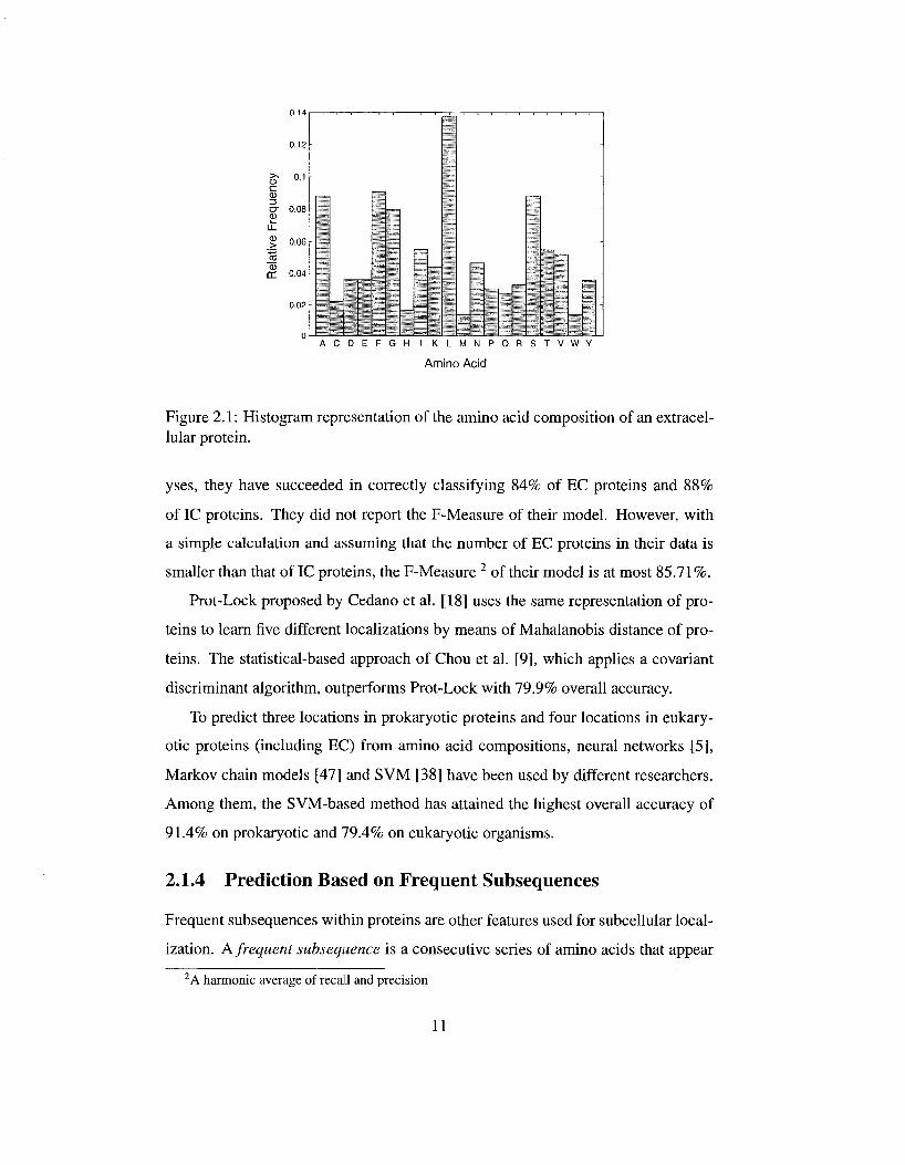
Acid Composition" of a protein and results in a 20-dimensional dataset. Figure 2.1
illustrates such a representation for an EC protein.
Nakashima et al. [15] have found discrimination between EC and IC proteins
by amino acid compositions and residue-pair frequencies. Based on statistical anal-
10
I ,1 i i , I I -I. I I I I. I t i i II F G H I K L M N P Q R S T V W Y
Amino Acid
Figure 2.1: Histogram representation of the amino acid composition of an extracellular protein.
yses, they have succeeded in correctly classifying 84% of EC proteins and 88%
of IC proteins. They did not report the F-Measure of their model. However, with
a simple calculation and assuming that the number of EC proteins in their data is
smaller than that of IC proteins, the F-Measure 2 of their model is at most 85.71 %.
Prot-Lock proposed by Cedano et al. [18] uses the same representation of pro
teins to learn five different localizations by means of Mahalanobis distance of pro
teins. The statistical-based approach of Chou et al. [9], which applies a covariant
discriminant algorithm, outperforms Prot-Lock with 79.9% overall accuracy.
To predict three locations in prokaryotic proteins and four locations in eukary-
otic proteins (including EC) from amino acid compositions, neural networks [5],
Markov chain models [47] and SVM [38] have been used by different researchers.
Among them, the SVM-based method has attained the highest overall accuracy of
91.4% on prokaryotic and 79.4% on eukaryotic organisms.
2.1.4 Prediction Based on Frequent Subsequences
Frequent subsequences within proteins are other features used for subcellular local
ization. A frequent subsequence is a consecutive series of amino acids that appear
2 A harmonic average of recall and precision
>• 0.1
(1) - I n-<!> LL
> CO CD
DC
II OH
0.06
0.04
11
in more than a certain number of proteins of a specific class. In this context, pro
teins are represented in terms of frequent subsequences they contain. Zai'ane et
al. [48] used such features and applied SVM and boosting methods to predict EC
localization. Their highest F-Measure is 80.4% when SVM is used. In another
effort, they have used discriminative frequent sequential patterns as rules [48]. A
frequent sequential pattern is of the form *X\ *X2* ... * Xn* where Xt is a frequent
subsequence and * represents a variable-length-don't-care. The same method for
localizing Outer Membrane (OM) proteins has been used by She et al. [36]. Their
rule-based classifier "has very good performance in terms of OM class precision
(well over 90%), however, the corresponding recall is low (around 40%)" [36].
2.1.5 Prediction Based on Integrative Approaches
The last category of approaches is the combination of different methods. The previ
ous work on predicting extracellular plant protein localization, by Zai'ane et al. [48],
applies a boosting algorithm on proteins where each protein is represented by a
combination of its frequent subsequences and its amino acid composition. Their
approach has reached an F-Measure of 83.1%, which is outperformed by the 5%
higher F-Measure of our method. With SVM as the learning algorithm, Li and
Liu [42] predict protein locations by combining N-terminal signals and amino acid
compositions. Their highest achievement is 91.9% overall accuracy on non-plant
proteins. Hoglund et al. haive achieved the overall accuracy of more than 74% by
combining N-terminal signals, amino acid compositions and sequence motifs [4].
PSORT [23], probably the most complete tool for predicting many different lo
calization sites, integrates various statistical methods and classification algorithms.
However, its overall accuracy is less than 66%.
2.1.6 Challenges and Limitations of the State-of-the-Art Methods
What motivates us to proceed with the research idea of this dissertation is the pres
ence of some limitations in the algorithms mentioned above, specially when they
are considered for the case of EC localization prediction. The deficiency of these
12
algorithms highlights the need for our research and the suitability of the algorithm
proposed in this research. In the following, the limitations of the-state-of-the-art
methods are listed:
• Because of the important role of EC proteins in plants, it is valuable for bi
ologists to access solutions for predicting such proteins. Therefore, our work
particularly focuses on discriminating EC and IC proteins, while most of the
existing algorithms are not well-devised and suitable for this purpose.
• Some of the state-of-the-art algorithms suffer from either low precision or low
recall. However, most time the overall classification accuracy of the models
is reported which is often a higher measure. For example, in the case of
our problem, a classifier that always classifies as IC will have a recall and F-
Measure of zero while the overall accuracy of such a classifier is 96% because
EC proteins are only 4% of the entire plant protein dataset. Therefore, overall
accuracy is not as informative as F-Measure. Our work tries to increase both
recall and precision at the same time so that both a high F-measure and high
overall accuray is achieved.
• Our approach tackles a hard and challenging binary classification in which
there is a high imbalance between the number of samples of the two classes
(EC and IC). Handling such an imbalance is not a matter of attention in many
of the approaches.
• In most cases, the algorithms fail to present a justification of their prediction.
A biologist may not rely on the results of a neural network or an SVM classi
fier if they need some tangible and understandable biological facts extracted
by the prediction models. Using the associative classifier in our research
helps to acquire not a black-box classifier but a set of accurate, small and in-
terpretable localization rules that can be used for further biological analyses.
Moreover, our secondary classifier, nearest neighbor classifier, is biologically
justified when the distance of proteins is based on edit distance. The reason
is that amino acid deletions, insertions, substitutions (mutations) along pro-
13
tein sequences happen through biochemical processes, and these three are the
permitted operations in the computation of edit distance.
• Partition-Based Subsequence (PBS) is a novel type of protein features that has
never been proposed before. By using PBSs, we probably indirectly exploit
information about the folded structures of proteins in prediction, something
that is not considered in the mentioned works.
• Some algorithms are the solutions to specific problems and cannot be ex
tended to a complete localization problem in which learning all the possible
localizations is targetted. For example, TargetP cannot classify beyond ex
tracellular, mitochondria and chloroplast, as all proteins that cannot fall in
any of the three localization classes are classified as "other". The specific
localizations in "other" proteins cannot be learnt by the approach of TargetP.
In contrast, our approach, although not experimentally confirmed yet for the
complete localization prediction, has the potential to tackle multi-class local
ization problems (Refer to Future Work section).
2.2 Work Related to Frequent Subsequence Mining
There are different approaches to mine frequent subsequences of a given length and
a minimum frequency or support (MinS up). A naive solution is shown in Figure 2.2
that recursively builds subsequences and counts their support. This algorithm can
handle only small datasets that can fit in main memory. It needs a large memory
in the case of mining long subsequences when the recursive function goes too far
deep.
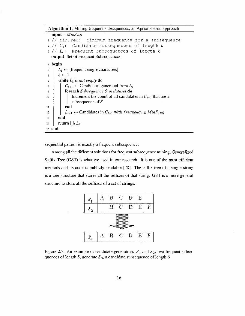
As another solution for subsequence mining, an APriori-based approach is pro
posed. Frequent subsequences meet the apriori property, i.e.,if a subsequence S [l...n]
of length n is frequent, subsequences S[l...n - 1] and S[2...n] are frequent too.
Therefore, this algorithm first mines frequent subsequences of length 1. Induc
tively, to mine frequent subsequences of length n + 1, subsequences S[l...n] and
Q[\...ri\ of length n where S [2...n] = Q[l...n - 1] combine and create a candidate
14
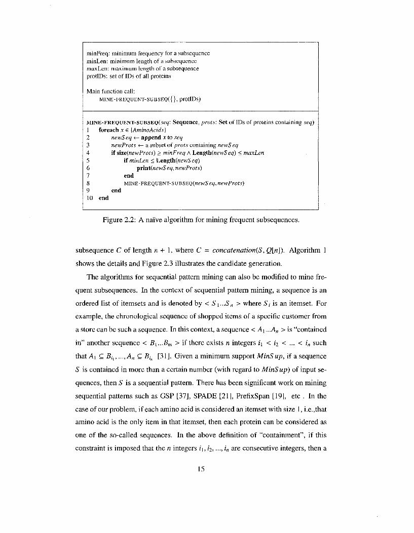
minFreq: minimum frequency for a subsequence minLen: minimum length of a subsequence maxLen: maximum length of a subsequence protlDs: set of IDs of all proteins
Main function call: MINE-FREQUENT-SUBSEQ({},protIDs)
MINE-FREQUENT-SUBSEQ(5eg: Sequence, prots: Set of IDs of proteins containing seq) 1 foreach x e {AminoAcids] 2 newSeq <— append x to seq 3 newProts «— a subset of prots containing newSeq 4 if size(newProts) > minFreq A L,ength(newS eq) < maxLen 5 ii minLen < Length(newS eq) 6 print(«e wS eq, newProts) 7 end 8 MiNE-FREQUENT-sUBSEQ(«ewSe<7, newProts) 9 end 10 end
Figure 2.2: A naive algorithm for mining frequent subsequences.
subsequence C of length n + 1, where C = concatenation's, Q\n\). Algorithm 1
shows the details and Figure 2.3 illustrates the candidate generation.
The algorithms for sequential pattern mining can also be modified to mine fre
quent subsequences. In the context of sequential pattern mining, a sequence is an
ordered list of itemsets and is denoted by < S\...Sn > where S, is an itemset. For
example, the chronological sequence of shopped items of a specific customer from
a store can be such a sequence. In this context, a sequence < A\ ...An > is "contained
in" another sequence < B\...Bm > if there exists n integers i\ < ii < ... < in such
that A\ c Bit, ...,A„ c Bin [31]. Given a minimum support MinSup, if a sequence
S is contained in more than a certain number (with regard to MinS up) of input se
quences, then S is a sequential pattern. There has been significant work on mining
sequential patterns such as GSP [37], SPADE [21], PrefixSpan [19], etc . In the
case of our problem, if each amino acid is considered an itemset with size 1, i.e.,that
amino acid is the only item in that itemset, then each protein can be considered as
one of the so-called sequences. In the above definition of "containment", if this
constraint is imposed that the n integers i\, i2,..., in are consecutive integers, then a
15
Algorithm 1: Mining frequent subsequences, an Apriori-based approach input : MinS up
1 / / MinFreq : Minimum f r e q u e n c y f o r a s u b s e q u e n c e i l l Ck'. C a n d i d a t e s u b s e q u e n c e s of l e n g t h k 3 / / Lk'. F r e q u e n t s u b s e q u e n c e s of l e n g t h k
output: Set of Frequent Subsequences
4 begin 5
6
7
8
9
10
11
12
13
14
L l *-- {frequent single characters) k*~ 1 while Lk is not empty do
Ck+i <— Candidates generated from Lk
foreach Subsequence S in dataset do Increment the count of all candidates in Ck+i that are a subsequence of S
end Lk+i <— Candidates in Ck+\ with frequency > MinFreq
end rt Jtun nil***
is end
sequential pattern is exactly a frequent subsequence.
Among all the different solutions for frequent subsequence mining, Generalized
Suffix Tree (GST) is what we used in our research. It is one of the most efficient
methods and its code is publicly available [20]. The suffix tree of a single string
is a tree structure that stores all the suffixes of that string. GST is a more general
structure to store all the suffixes of a set of strings.
sl
s2
A B C
B C
D E
D E F
A3 O A B C D E F
Figure 2.3: An example of candidate generation. Si and S2, two frequent subsequences of length 5, generate S 3, a candidate subsequence of length 6
16
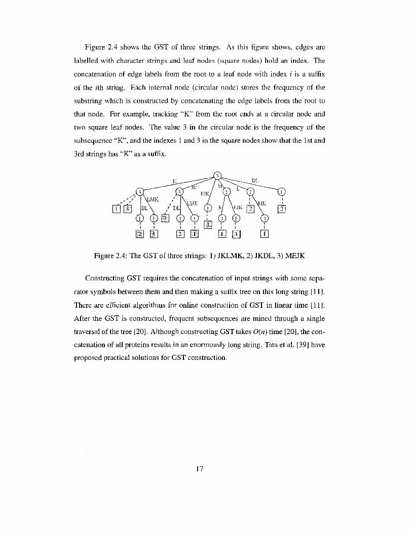
Figure 2.4 shows the GST of three strings. As this figure shows, edges are
labelled with character strings and leaf nodes (square nodes) hold an index. The
concatenation of edge labels from the root to a leaf node with index i is a suffix
of the zth string. Each internal node (circular node) stores the frequency of the
substring which is constructed by concatenating the edge labels from the root to
that node. For example, tracking "K" from the root ends at a circular node and
two square leaf nodes. The value 3 in the circular node is the frequency of the
subsequence "K", and the indexes 1 and 3 in the square nodes show that the 1st and
3rd strings has "K" as a suffix.
I I I I -! I I I I I I I I * I I I I
mm mm mm m Figure 2.4: The GST of three strings: 1) JKLMK, 2) JKDL, 3) MEJK
Constructing GST requires the concatenation of input strings with some sepa
rator symbols between them and then making a suffix tree on this long string [11].
There are efficient algorithms for online construction of GST in linear time [11].
After the GST is constructed, frequent subsequences are mined through a single
traversal of the tree [20]. Although constructing GST takes 0(n) time [20], the con
catenation of all proteins results in an enormously long string. Tata et al. [39] have
proposed practical solutions for GST construction.
17
Chapter 3
Protein Feature Extraction
A protein, in a simple 1-dimensional representation, is a sequence of amino acids.
It needs to be represented by a set of features in order to be in a suitable format for
learning algorithms. A feature dataset can be in a relational or transactional format.
In transactional format, a protein is in the form of a set of specific features, e.g.,
frequent subsequences, extracted from that protein. These sets are not necessarily
of the same size. In order to transform such data to a relational format, data is
organized in a table structure where each column corresponds to a feature, and rows
represent proteins. In this format, a protein is assigned a value of 1 at a column if
the protein possesses the feature related to that column; otherwise, 0.
If the original format of data is relational, e.g., the case where proteins are
represented by their amino acid compositions, a transactional format can be simply
obtained by discretizing all the continuous attributes, assiging unique codes to each
attribute-value pair, and representing each protein by the set of the codes of their
attribute-value pairs.
Since in this research, an associative classifier is used for learning and predicting
the protein localizations, and associative classifiers deal with data in transactional
format, the feature datasets should be transactional. To find out whether a feature
set is suitable for localization prediction, an associative classifier is applied on the
feature dataset. If a high prediction accuracy is achieved, the extracted features are
satisfactory; otherwise, other types of features should be studied. It is possible for a
feature dataset not to be well learnt by associative classifiers while another classifier
could learn the same dataset better. However, the accuracy of associative classifier
18
is our main criterion for the suitability of extracted features since our ultimate goal
is building an interpretable and accurate model using strongly confident associative
rules.
In this work, we focus on two types of features:
• Frequent subsequences or FS.
• Frequent Partition-Based Subsequences or PBS, subsequences that are frequent in some discovered partitions of protein sequences.
The reason why our focus is on subsequence-based features is based on the
following observations:
• "Common subsequences among related proteins may perform similar functions via related biochemical mechanisms" [36] and are of great interest to biologists.
• "Frequent subsequences capture local similarity that may relate to important functional or structural information of extracellular proteins" [43].
Therefore, it is expected that frequent subsequences of proteins or "motifs" can
better discriminate proteins of different localization.
The following sections, elaborate on these features. Section 3.1 is a history of
the algorithms we tried to represent proteins by their FS features. At each step, a
deficiency of the algorithm is observed and the next algorithm aims at resolving it.
The series of different approaches are evolved until the algorithm for mining PBSs
is devised. The explanation about PBSs is brought in Section 3.2
3.1 History of Frequent-Subsequence-Based Feature Mining Algorithms
As discussed in Chapter 2, there are different approaches to mine frequent sub
sequences. However, because of the availability and efficiency of the GST-based
subsequence mining code [20], this algorithm is used. The important parameters of
this algorithm are:
• MinS up: The minimum support of a subsequence to be frequent. Support of
a subsequence S is the fraction of protein sequences that contain S
• MinLen: The required minimum length of a subsequence
19
• MaxLen: The required maximum length of a subsequence
After mining frequent subsequences, each protein is represented by the frequent
subsequences it contains, and a transactional feature dataset is built. Although
building such a feature dataset seems straightforward, our experiments on the plant
protein dataset showed many unexpected problems and difficulties. These problems
can be summarized in three categories:
1. The first and main problem is the imbalance between the size of EC and IC
proteins (127 vs. 3,022). Because of the diversity in the larger group, it is
very likely for the proteins in that group to contain the frequent subsequences
of the smaller group. It causes the subsequences of EC proteins to be less
distinctive, i.e., features from the rare EC group are not frequent enough to
be captured.
2. Another problem is that the resulted feature dataset may contain large trans
actions of hundreds of items. It is a serious problem for an associative clas
sifier to handle large transactions. In this case, the number of outputted rules
is so huge that processing them is sometimes impossible with the available
equipment. Long transactions are generated when mined subsequences are so
much frequent that each protein contains a significant number of them. Thus,
any subset of subsequences, which is potentially a rule, is probably frequent.
Therefore, a control is required over the length of the resulted transactions
during the whole process of frequent subsequence mining.
3. The last problem is the existence of silent proteins in the feature datasets.
Silent is referred to a protein that does not contain any of the frequent subse
quences that were extracted, i.e.,all their subsequences have low frequency.
On the other hand, lower frequencies lead to mining a huge number of subse
quences, which is hard to process.
Facing all these problems and attempting to resolve them, the algorithm of
building a subsequence-based feature dataset gets gradually evolved by different
modifications. The following sections explain different steps of the evolution of
our algorithm.
20
3.1.1 Class-Specific Subsequence Mining
In our dataset, 127 proteins are EC and 3,022 proteins are IC. It means that EC
proteins represent almost only 4% of the dataset. Thus, in mining frequent subse
quences, if MinSup is more than 4%, no subsequence specific to EC proteins is
found. On the other hand, MinS up of less than 4% is very low for the IC class with
abundant proteins, and thus a huge number of frequent subsequences are generated
which makes the later processings complex.
To solve this problem, subsequence mining is no longer done on the whole
protein set. Instead, it is done separately on the proteins of each class. This is
a fair modification because at a fixed input of MinS up, the frequency threshold
is proportional to the size of each dataset. Thus, at different ranges of MinS up,
frequent subsequences of each class have the chance to emerge.
3.1.2 M-Most Frequent Subsequences
Given a MinS up by which few or no silent proteins exist, such a large set of motifs
are found that the average size of transactions in the feature dataset becomes very
large \ which is hard for associative classifiers to process. Therefore, there should
be a limit on the number of mined motifs. A parameter "M" that selects M most
frequent subsequences can be a simple modification. A good selection of short
motifs, i.e.,length 3 or 4, results in an accurate classifier, however, there are some
drawbacks to this model. First, these short motifs are common in both classes.
Thus, they are not class-distinguishing by their own, and it is the association of
motifs that discriminates classes. Moreover, this model lacks flexibility in the length
of the motifs. With motifs of higher length, many silent proteins appear because
some proteins contain the M-most frequent subsequences even for large values of
M such as 1000. Hence, in the feature dataset, this particular set of expressed
proteins becomes long transactions of size around M, while the rest of the proteins
are silent.
'Experimentally (in the environment that is explained in the experimental study section), if the average size of transactions exceeds 30, the number of rules produced by associative classifier and the execution time fall in the scale of milions and days respectively.
21
Henceforth, we refer to motifs of length less than 5 as SHORT and higher length
motifs as LONG. In the future algorithms we focus on mining long motifs.
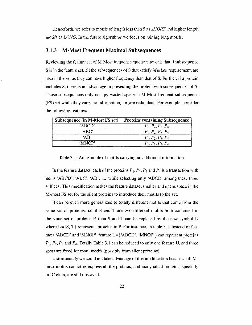
3.1.3 M-Most Frequent Maximal Subsequences
Reviewing the feature set of M-Most frequent sequences reveals that if subsequence
S is in the feature set, all the subsequences of S that satisfy MinLen requirement, are
also in the set as they can have higher frequency than that of S. Further, if a protein
includes S, there is no advantage in presenting the protein with subsequences of S.
Those subsequences only occupy wasted space in M-Most frequent subsequence
(FS) set while they carry no information, i.e.,are redundant. For example, consider
the following features:
Subsequence (in M-Most FS set) 'ABCD' 'ABC 'AB'
'MNOP'
Proteins containing Subsequence P 1 . P 2 . P 3 . P 4
•P1.-P2.-P3.-P4
P 1 . P 2 . P 3 . P 4
P 1 . P 2 . P 3 . P 4
Table 3.1: An example of motifs carrying no additional information.
In the feature dataset, each of the proteins P\,Pi, P3 and P4 is a transaction with
items 'ABCD', 'ABC, 'AB', .... while selecting only 'ABCD' among these three
suffices. This modification makes the feature dataset smaller and opens space in the
M-most FS set for the silent proteins to introduce their motifs to the set.
It can be even more generalized to totally different motifs that come from the
same set of proteins, i.e.,if S and T are two different motifs both contained in
the same set of proteins P, then S and T can be replaced by the new symbol U
where U={S, T} represents proteins in P. For instance, in table 3.1, instead of fea
tures 'ABCD' and 'MNOP', feature U={ 'ABCD', 'MNOP'} can represent proteins
P\,P2, Pi and P4. Totally Table 3.1 can be reduced to only one feature U, and three
spots are freed for more motifs (possibly from silent proteins).
Unfortunately we could not take advantage of this modification because still M-
most motifs cannot re-express all the proteins, and many silent proteins, specially
in IC class, are still observed.
22
3.1.4 N-Most Discriminative Motifs
Instead of filtering motifs by selecting the M-most frequent ones, they can be fil
tered by selecting the N-most discriminant motifs. Given a MinSup and MinLen,
all motifs are mined separately from each class. If a motif is frequent in one class
and also appears in another class, it is not considered discriminant. Based on this
criterion, coincidence degree of a subsequence of a class is defined as an indicator
of the appearance of that subsequence in the opposite class. In this algorithm, if
a motif is discriminant, its coincidence degree is zero; otherwise, one. Of the dis
criminant motifs, N most frequent ones are selected to make the feature dataset. If
they are less than N, we have to select out of the non-discriminant motifs.
This modification still suffers from silent proteins. Even if the value of N is set
close to the whole number of mined motifs silent proteins will show up (even at low
MinS up)
3.1.5 N-Most Discriminative Motifs Based on IC Localizations
Based on the fact that proteins of a same localization present higher similarity, it
might be a good idea not to put all the intracellular proteins in only one group of
IC. They can be grouped as the proteins of nucleus, mitochondria, etc . In this
way, features of each type of intracellular proteins are independently captured, and
it is expected that more proteins become expressed. In the previous algorithm, if
a motif of a class does not appear in the other class, it is considered discriminant
and receives a coincidence degree of 0, otherwise 1. Here in this algorithm, instead
of mining motifs of EC and IC proteins, motifs of each of the 9 IC localizations
(mentioned in Section 1.1) and the EC localization are mined separately and the
coincidence degree of each motif, which is now an integer between 0 and 9, is com
puted. Afterwards, all the motifs derived from proteins of classes other than EC
are collected as the motif set of IC class. Then N-most discriminant motifs (having
lowest coincidence degrees) are selected from the motif set of each class and the
feature dataset is constructed based on the union of the two motif sets. The result
of this algorithm is more frustrating because many of IC proteins appear silent. The
23
reason is that at some IC localizations, a few proteins exist whose frequent subse
quences can not be well learnt. For example, peroxisomal contains only 29 proteins
which is a very few number of training samples, and learning the pattern of per
oxisomal proteins based on frequent subsequences can not be accurate. Moreover,
proteins of the nine IC classes are very similar in terms of their structure and se
quences. Therefore, the frequency of IC frequent motifs is accumulated over the
nine different classes. Dividing IC proteins into 9 separate classes, breaks down the
frequency of those motifs and they fail to reach the minimum frequency in this al
gorithm. Based on this experience and the inferences, the next algorithms consider
all proteins of the nine IC localizations as a whole.
Protein ID
Px
•Pi 998
A 999
•f*2000
•^2331
^ 2 3 3 2
^ 2 3 3 3
-P3149
Symbolic Presentation of The Features
# * * 1 > Small number of motifs (short transaction-like proteins)
* * I
innniinniinir*** * * * * * * * * * * * * * * * * * * * * *
Large number of motifs representing around 330 IC(chloroplast) proteins (long transaction-like proteins)
* 1 • • • \ Small number of motifs (short transaction-like proteins)
* * J
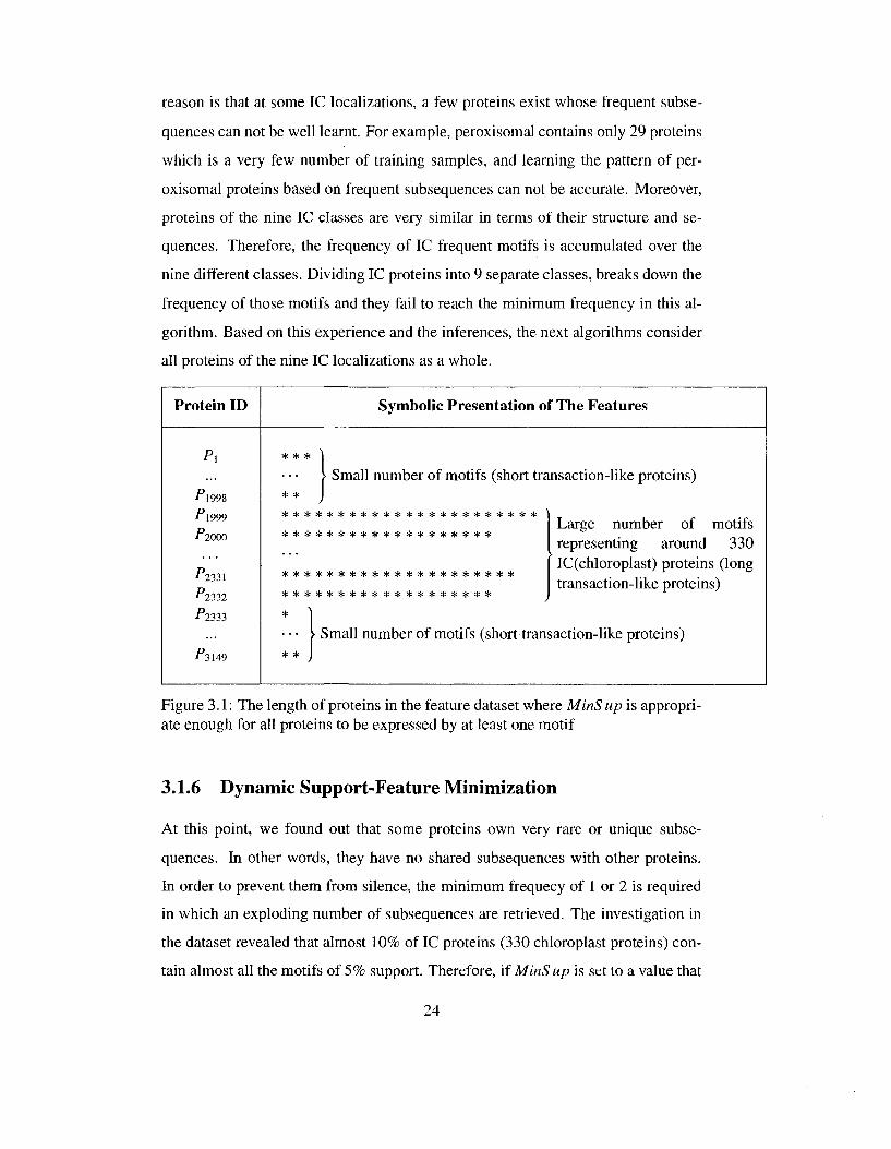
Figure 3.1: The length of proteins in the feature dataset where MinSup is appropriate enough for all proteins to be expressed by at least one motif
3.1.6 Dynamic Support-Feature Minimization
At this point, we found out that some proteins own very rare or unique subse
quences. In other words, they have no shared subsequences with other proteins.
In order to prevent them from silence, the minimum frequecy of 1 or 2 is required
in which an exploding number of subsequences are retrieved. The investigation in
the dataset revealed that almost 10% of IC proteins (330 chloroplast proteins) con
tain almost all the motifs of 5% support. Therefore, if MinS up is set to a value that
24
Silent Extracellular Proteins vs. Minimum Support Extracellular Long Motifs vs. Minimum Support
MinSup (%) MinSup (%)
Silent Intracellular Proteins vs. Minimum Support Intracellular Long Motifs vs. Minimum Support
MinSup (%) MinSup (%)
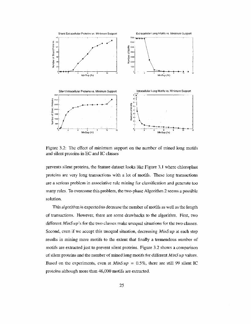
Figure 3.2: The effect of minimum support on the number of mined long motifs and silent proteins in EC and IC classes
prevents silent proteins, the feature dataset looks like Figure 3.1 where chloroplast
proteins are very long transactions with a lot of motifs. These long transactions
are a serious problem in associative rule mining for classification and generate too
many rules. To overcome this problem, the two-phase Algorithm 2 seems a possible
solution.
This algorithm is expected to decrease the number of motifs as well as the length
of transactions. However, there are some drawbacks to the algorithm. First, two
different MinSup's for the two classes make unequal situations for the two classes.
Second, even if we accept this unequal situation, decreasing MinS up at each step
results in mining more motifs to the extent that finally a tremendous number of
motifs are extracted just to prevent silent proteins. Figure 3.2 shows a comparison
of silent proteins and the number of mined long motifs for different MinS up values.
Based on the experiments, even at MinSup = 0.5%, there are still 99 silent IC
proteins although more than 46,000 motifs are extracted.
25
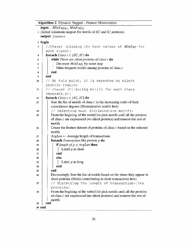
Algorithm 2: Dynamic Support - Feature Minimization
input : MinSupEc, MinSupic 1 (Initial minimum support for motifs of EC and IC proteins)
output: features
2 begin //Phasel (Finding the best values of MinSup for each class): foreach Class c e {EC, IC) do
while There are silent proteins of class c do Decrease MinS upc by some step Mine frequent motifs among proteins of class c
end end // At this point, it is expected no silent protein remains // Phase2 (Filtering motifs for each class separately): foreach Class c e {EC, IC} do
Sort the list of motifs of class c in the increasing order of their coincidence degrees (Dicriminative motifs first) // Selecting most dicriminative motifs: From the begining of the sorted list pick motifs until all the proteins of class c are expressend (no silent proteins) and remove the rest of motifs Create the feature dataset of proteins of class c based on the selected motifs AvgLen <— Average length of transactions foreach Transaction-like protein p do
if length of p < AvgLen then | Label p as short
end else | Label p as long
end end Decreasingly Sort the list of motifs based on the times they appear in short proteins (Motifs contributing to short transactions first) // Minimizing the length of transaction-like proteins: From the begining of the sorted list pick motifs until all the proteins of class c are expressend (no silent proteins) and remove the rest of motifs
end 30 end
26
Based on Figure 3.2, the fewer silent proteins, the more motifs. Hence, a com
pressing data structure should be used to store motifs and the Id of their proteins in
order for further processing. A "Trie" may be the best candidate of such a struc
ture. "Trie" is a tree structure where the internal nodes hold alphabetic characters
and the nodes of each level are alphabetically sorted. Trie is mainly used to store
a dictionary of words with a fast search possibility. A path from the root to a leaf
constitutes a word. In our case, if 'X' is a motif of length n, it corresponds to a
node at level n. This node maintains the set 5 of IDs of the proteins that contain the
corresponding motif. If 'Xa' is also a motif where 'a' is just a single character (one
amino acid), the corresponding node contains set T of IDs such that T c S. Thus,
the members of T should be removed from S to avoid repetitive information. In this
way, lots of memory is saved.
All of these problems motivate for alternative solutions to be considered.
3.1.7 Dynamic Support - Rare Motif Detection
According to our previous experiments, it was found out that some proteins do not
contain frequent motifs, i.e.,remain silent. All their motifs are unique to them or
very rare. These rare motifs can be considered important as they identify proteins
with uncommon or specific patterns, probably with special properties. As we ex
plained in the previous section, setting MinSup to small values for mining rare
motifs is not appropriate as it makes normal proteins expressed with their frequent
as well as rare motifs. Therefore, extra information will be produced. Algorithm 2,
mentioned in the previous secion, can be simply modified such that frequent mo
tifs and useful rare motifs are extracted separately. In this modification, an initial
MinS up (to be the criterion of "frequentness") is given to each class and frequent
motifs are mined. Then for each class, the proteins are separated into two sets:
those that are expressed by the frequent motifs, S i and those that are not, 52- Now
algorithm 2 is applied to all proteins, but of the newly generated motifs, only those
representing at least one protein of set S 2 are kept and the rest are ignored. There
fore, if a protein is already expressed by some motif, it is not re-expressed by newly
mined motifs (with lower supports) and many useless motifs are filtered.
27
Figure 3.2 helps to set initial MinS up of each class. In an experiment, the initial
MinSup of 4% and 10% were selected for motifs of EC and IC class respectively.
In mining rare motifs, it was proven that the minimum absolute frequency of 2 is
needed for some proteins to be expressed; otherwise, they remain silent. In this
case, although rare motifs only from set S2 are supposed to be extracted, more than
50,000 motifs with absolute support of 2 or more appear.
3.1.8 Dynamic Support - Most Discriminative Frequent Motif
To filter more motifs, the previous algorithm can be modified as follows:
Of the different motifs that express a protein P, P has to pick only the motif
with the highest score. Score can be frequency, length, or a weighted sum of them,
etc . When a new motif is mined, all the proteins containing that motif compare its
score with the score of the motif they have already had. A protein replaces its older
motif with the new one if a higher score is obtained.
This algorithm does not guarantee that the length of each transaction in the
feature dataset is 1. For example, a protein Pi may contain motifs Mi and M2 but
only M\ is its best motif. On the other side, M2 may be the best motif of another
protein P2. Although P\ and P2 each select one motif, but in the end, since both
motifs are kept in the mined feature set, Pi has to be also represented by M2. Due
to this fact, long transactions still persist. A bigger problem is that silent proteins
are avoided in return for decreasing MinSup to very small values. It causes some
proteins to be only expressed by very rare motifs. Later, an associative classifier
generates no rule to classify such proteins because it finds frequent rules based on
frequent motifs. In the next section (3.1.9) we explain and solve this problem.
3.1.9 N-Best (Longest) Motifs
Since this project develops a classification model, and a classifier represents a gen
eral (frequent) pattern of data, we could state that only general (frequent) motifs
are needed. Although decreasing MinSup lessens the number of silent proteins,
rare motifs cannot contribute to classification rules, which are frequently observed
relations between data and classes. Later on, test proteins expressed by rare motifs
28
cannot be classified. We should adopt the fact that there is no frequent and long
motif for some proteins (silent proteins) and rare long motifs seem useless at the
end. On the other hand, we are interested in long motifs although frequent short
motifs can express all proteins, as mentioned previously in section 3.1.2. These two
ambitions (high length and frequency) are considered in the following approach:
Input an integer N and only one desirable MinS up value (the same MinS up
for both EC and IC). Throughout the algorithm, MinS up is never changed, but the
length of the motifs to be mined decreases until no silent protein remains. Each
protein is supposed to be expressed with at most N best motifs. Selecting the best
motifs is based on a score that is defined as a function of length, frequency, number
of occurrences in the other class, etc . The simplest way is to assign higher scores
to longer motifs and if motifs are equally long, to those that are more discriminant
(fewer occurrences in the other class). The details are shown in Algorithm 3.
In this algorithm, proteins start selecting their motifs from the longest ones.
Length is a good selection criterion because longer motifs may contain more infor
mation than short ones. Moreover, "with the alphabet of only 20 amino acids, it is
likely that very short subsequences will occur in sequences of both classes and such
subsequences are non-discriminative with regard to classification" [36].
Based on this algorithm, a protein is marked as NeedingMotif when it is not
yet expressed by N motifs. To find a setting for N, if it is set to 1, then only the
proteins that are completely silent are marked as NeedingMotif. Experimentally
we observed that all the proteins can be expressed by frequent motifs not shorter
than 3.
As compared to the previous algorithms, this algorithm has a more reliable strat
egy to find discriminative motifs. Previously, coincidence degree of only 0 or 1 was
assigned to motifs to indicate if it is discriminant. Then, motifs were filtered based
on this degree. It sounds unfair because if a motif is very frequent in its own class
and appears only once in the other class, it is considered as non-discriminent and
is filtered while it should not be. Therefore, instead of 0 and I, the frequency of
the motif in the other class is taken into account. In Algorithm 3, for each motif
two frequencies related to each class are available, namely fEc and fIc. US is a
29
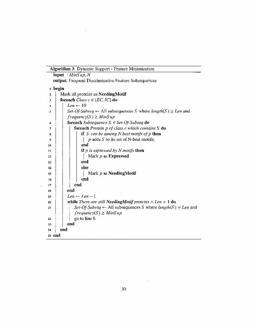
Algorithm 3: Dynamic Support - Feature Minimization input : MinSup,N output: Frequent Discriminative Feature Subsequences
1 begin Mark all proteins as NeedingMotif foreach Class c e {EC, IC] do
Len <- 10 Set-Of-Subseq <— All subsequences S where length(S) > Len and frequency(S) > MinSup foreach Subsequence S £ Set-Of-Subseq do
foreach Protein p of class c which contains S do if S can be among N best motifs of p then | p adds S to its set of N-best motifs;
end if p is expressed by N motifs then | Mark p as Expressed
end else | Mark p as NeedingMotif
end end
end Len <— Len - 1 while There are still NeedingMotif proteins A Len > 1 do
Set-Of-Subseq <— All subsequences S where length(S) - Len and frequency(S) > MinSup go to line 6
end end
25 end
30
frequent subsequence of EC class, the confidence of S is defined as the fraction of
proteins containing S that belong to EC class:
T PC
confidence(S) — — — (3.1) JEC + fie
and similarly for the motifs of IC class.
When finding motifs of a class, motifs with confidence less than a given thresh
old can be simply removed. This threshold is called MinConf (minimum con
fidence) and can be inputted as another parameter. If MinConf is set to 100%,
frequent motifs appearing only in one class (absolutely discriminative) are discov
ered.
The only problem that still remains, is the problem of long transactions as we
have already explained. However, the extensive efforts in this research demonstrates
that it is not wise to put more effort on controlling the length of transactions. In
stead, some solutions to increase the ability of the associative classifier for handling
long transactions should be explored. These solutions and techniques are elaborated
in chapter 4.
3.2 Discriminative and Frequent Partition-Based Subsequences
Previous section concluded with an approach to discover the most discriminative
features based on only frequent subsequences or motifs. However, we believe that
the presence of a subsequence in special partitions of protein sequences might be
more discriminative than the subsequence itself. For example, "ACDE" may be a
frequent subsequence among both IC and EC proteins, thus is not distinguishing.
Nonetheless, "ACDE" may appear in the first half of EC protein sequences while in
IC proteins it may occur in the second half of the sequences. Here the association
of "ACDE" and its respective location along proteins is a discriminative pattern.
Such a pattern is called "Partition-Based Subsequence", or in short PBS. PBSs are
the generalized form of simple subsequences. Simple subsequences are the PBSs
whose partition is the whole protein.
31
Since proteins highly differ in length, the partition should be defined relative
to the length (partition-based) i.e.,a protein sequence is divided into 2, 3 or more
equal partitions. The presence of frequent subsequences in different partitions is
investigated. If protein sequences are assumed to be divided into P partitions, the
presence of a subsequence S in the f th partition of proteins, where 1 < i < P,
is denoted by S ,•//>. The problem is to find subsequences S with their partitions,
i.e.,values for i and P, such that £,•//> is frequent and discriminative with respect to
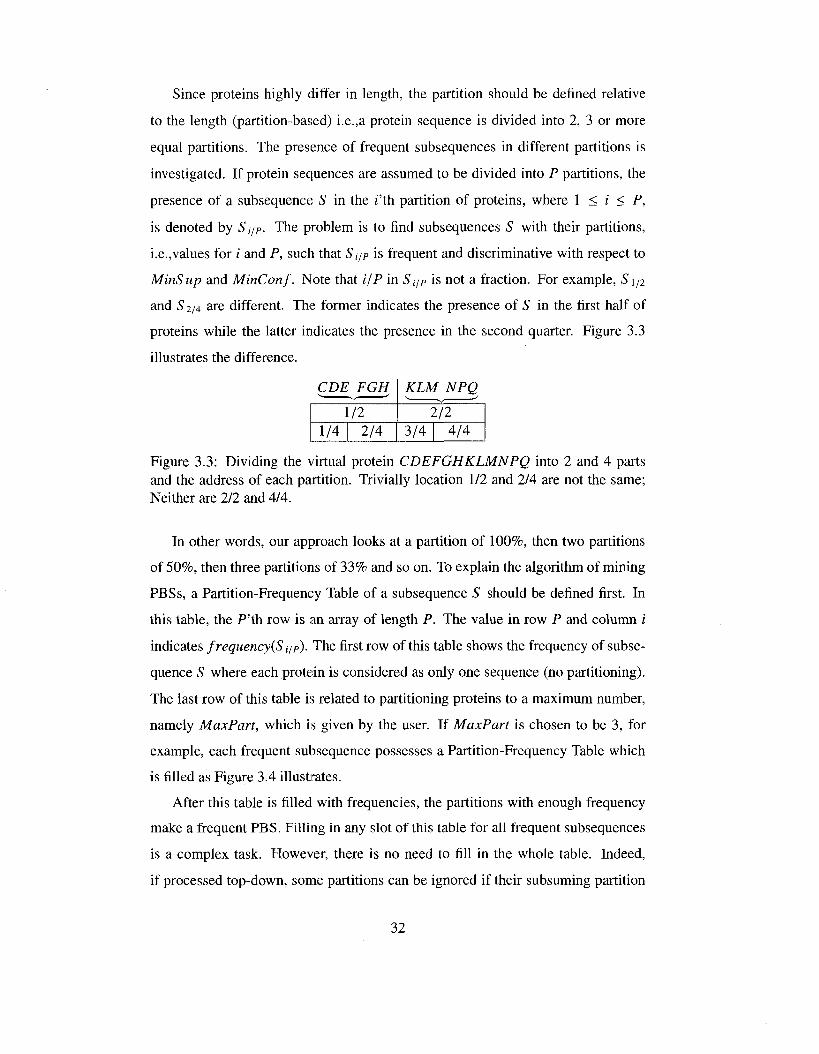
MinSup and MinConf. Note that i/P in S,y/> is not a fraction. For example, S1/2
and S 2/4 are different. The former indicates the presence of S in the first half of
proteins while the latter indicates the presence in the second quarter. Figure 3.3
illustrates the difference.
CDE FGH
1/2 1/4 2/4
KLM NPQ
2/2 3/4 4/4
Figure 3.3: Dividing the virtual protein CDEFGHKLMNPQ into 2 and 4 parts and the address of each partition. Trivially location 1/2 and 2/4 are not the same; Neither are 2/2 and 4/4.
In other words, our approach looks at a partition of 100%, then two partitions
of 50%, then three partitions of 33% and so on. To explain the algorithm of mining
PBSs, a Partition-Frequency Table of a subsequence S should be defined first. In
this table, the P'th row is an array of length P. The value in row P and column i
indicates frequency(S ,-//>). The first row of this table shows the frequency of subse
quence S where each protein is considered as only one sequence (no partitioning).
The last row of this table is related to partitioning proteins to a maximum number,
namely MaxPart, which is given by the user. If MaxPart is chosen to be 3, for
example, each frequent subsequence possesses a Partition-Frequency Table which
is filled as Figure 3.4 illustrates.
After this table is filled with frequencies, the partitions with enough frequency
make a frequent PBS. Filling in any slot of this table for all frequent subsequences
is a complex task. However, there is no need to fill in the whole table. Indeed,
if processed top-down, some partitions can be ignored if their subsuming partition
32
frequency{S) frequency(S 1/2) frequency (S1/3) frequency(S\/4)
frequency(S 2/2) frequency(S 2/3) frequency(S 2/4)
frequency(S 3/3) frequency(S 3/4) frequency(S 4/4)
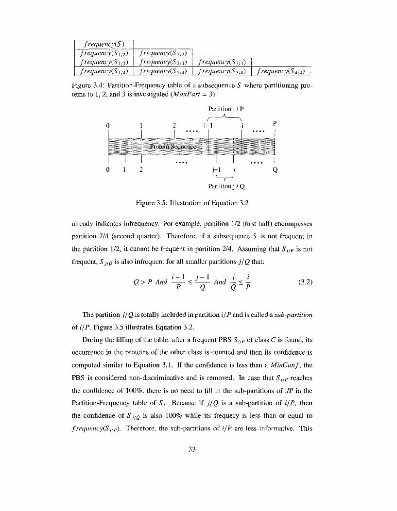
Figure 3.4: Partition-Frequency table of a subsequence S where partitioning proteins to 1, 2, and 3 is investigated (MaxPart = 3)
0 1
1 2 ! 1 * • • •
Protein Sequence
1 • * • •
2
Partition i t ^ ~
i-1
1
j - l J
Partition j
/P ^ i
1
/Q
"igure 3.5: Illustration of Equation 3.2
Q
already indicates infrequency. For example, partition 1/2 (first half) encompasses
partition 2/4 (second quarter). Therefore, if a subsequence S is not frequent in
the partition 1/2, it cannot be frequent in partition 2/4. Assuming that Syp is not
frequent, S J/Q is also infrequent for all smaller partitions j/Q that:
i — 1 / — 1 / i Q>P And < And — < -
P Q Q P
(3.2)
The partition j/Q is totally included in partition i/P and is called a sub-partition
of i/P. Figure 3.5 illustrates Equation 3.2.
During the filling of the table, after a frequent PBS Si/P of class C is found, its
occurrence in the proteins of the other class is counted and then its confidence is
computed similar to Equation 3.1. If the confidence is less than a MinConf, the
PBS is considered non-discriminative and is removed. In case that St/p reaches
the confidence of 100%, there is no need to fill in the sub-partitions of i/P in the
Partition-Frequency table of S. Because if j/Q is a sub-partition of i/P, then
the confidence of S J/Q is also 100% while its frequecy is less than or equal to
frequency(Si/p). Therefore, the sub-partitions of i/P are less informative. This
33
way, partitions are dynamically determined, and MaxPart is only an upper bound
for the partitions.
Because of the large number of frequent discriminative PBSs, and to reduce the
number of features, each protein is restricted to pick only N number of best PBSs
that match with it. If a PBS is not selected by any protein, it is removed. For
selecting its N best features, a protein ranks its PBSs based on different metrics.
In our approach, confidence, length and frequency are respectively the primary,
secondary and final ranking metric. For example, between two PBSs with equal
confidence, the longer one has a higher rank. Other metrics and priorities can be set
by the user depending on the importance of feature properties.
Algorithm 4 is a summary of what was discussed. If MaxPart is set to 1,
i.e.,proteins are considered as only one partition of 100%, the algorithm works
similar to Algorithm 3, explained in the previous section and only frequent sub
sequences regardless of partition are mined. However, there is a small difference
in the selection of N-best motifs. In Algorithm 3, the longer a protein is, the more
important it is to be selected by proteins. But in Algorithm 4, the priority is with
the most confident motifs as explained above. Experimentally, Algorithm 4 finds
better feature motifs in the case of maxPart - 1 than Algorithm 3.
As an advantage to our previous algorithms, this algorithm considers that ex
pressing test proteins is more important than expressing training proteins. If a test
protein remains silent in the resulted feature space, no rule can classify that protein
because rules are made up of features. We observed that some good features are
mined that can express a test protein P, but they are not among the N-best features
of the training proteins. Moreover, none of the N-best features of the training pro
teins express P. In such frequent cases, P remains silent if the N-best features of
only the training proteins build the feature space. Hence, each frequent and discrim
inative PBS, which is mined only based on the training proteins, is also given to the
test proteins matching with it. A test protein keeps that PBS if the PBS is among
the N-best features of the protein. Line 20 of Algorithm 4 is where this happens.
When proteins select their discriminative and frequent features, a union of PBSs
of all the training (EC and IC class) and unlabelled test proteins is made, and then
34
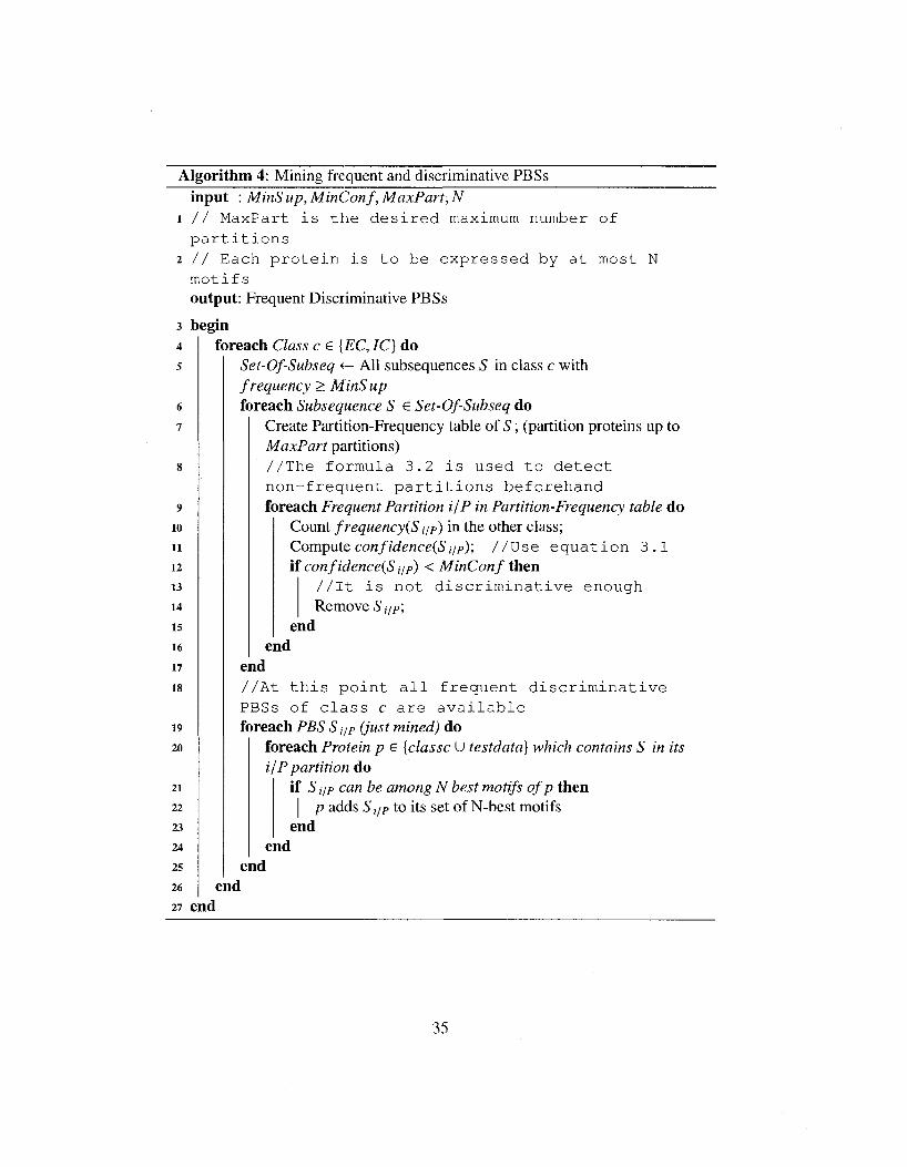
Algorithm 4: Mining frequent and discriminative PBSs input : MinS up, MinConf, MaxPart, N
1 // MaxPart is the desired maximum number of partitions
2 // Each protein is to be expressed by at most N motifs output: Frequent Discriminative PBSs
3 begin foreach Class c e {EC, IC} do
Set-Of-Subseq <— All subsequences S in class c with frequency > MinS up foreach Subsequence S e Set-Of-Subseq do
Create Partition-Frequency table of S; (partition proteins up to MaxPart partitions) / / T h e f o r m u l a 3 . 2 i s u s e d t o d e t e c t n o n - f r e q u e n t p a r t i t i o n s b e f o r e h a n d foreach Frequent Partition i/P in Partition-Frequency table do
Count frequency's t/p) in the other class; Compute confidence(S UP); / / U s e e q u a t i o n 3 . 1 if confidence's UP) < MinConf then
/ / I t i s n o t d i s c r i m i n a t i v e enough RemoveS,//-;
end end
end / /A t t h i s p o i n t a l l f requent d i s c r i m i n a t i v e PBSs of c l a s s c a r e a v a i l a b l e foreach PBS Si/P (just mined) do
foreach Protein p € {classc U testdata) which contains S in its i/P partition do
if 5 i/p can be among N best motifs of p then | p adds S i/p to its set of N-best motifs
end end
end end
27 end
35
proteins are represented by the PBSs from the union set with which they can match.
The feature dataset will be in the form of a transactional dataset. Afterwards, test
proteins that are still silent request for reconsideration. In the reconsideration pro
cess, a silent protein gets expressed by the PBSs from the union set that it can par
tially match. Test protein T is said to partially match with £,•//> if it cannot match
with this PBS but there exists a subsequence S' such that T and S'j/p can match and
EditDistance(S, S') = 1. Edit distance [11] is an appropriate metric for measuring
the amount of difference between two strings. Edit distance of 1 implies that 5 ' is
made by inserting a character to or deleting a character from S or by substituting a
character in S with another character. For example, if S - ABCD, S' is ABFCD,
ABD, AB1D or ... where '?' is a don't-care. More explanation about edit distance
is given in Section 4.2. According to our experiments, reconsideration reduces the
number of silent proteins by more then 10%.
The reason we chose the edit distance of 1, and not more, is that frequent sub
sequences are not very long. Roughly, their length varies from 3 to 10 in general.
With the above notation, Billowing more edit distances may lead to subsequences
S' that are no longer similar to the original subsequence S. More importanly, re
consideration is an expensive task and becomes more complex if the higher edit
distances are allowed. Our current approach for reconsideration includes creating
all subsequences S', for all PBSs Syp, and then checking all silent proteins if they
can match any S' in their i/P partition. As the length of S or the number of silent
proteins increase, more comparisons should be made.
36
Chapter 4
Associative Classification for Protein Localization
As the previous sections explained, the output of the feature extraction phase is
a transactional feature dataset. Different algorithms can be used to learn protein
localizations and classify unseen proteins to EC or IC localizations. However, a
classifier with interpretable output model is prefered. Moreover, if the accuracy of
such a classifier is high, two worthwhile goals are achieved: First, an accurate clas
sification model is found to predict the location of new unknown proteins. Second,
it can be inferred that a good selection of discriminative and descriptive features
of EC and IC proteins have been discovered. Although each transactional dataset
can be converted into relational format, it is better for the classifier to work with
transactional data since our feature datasets are originally transactional. If those
feature datasets are transformed to relational format, all the attributes become bi
nary (presence or absence of features). If such a dataset is n-dimensional, each
protein becomes a corner of the n-dimensional unit hyper-cube in the feature space.
Such data is very unlikely to be linearly or even easily separable and many classifi
cation algorithms may fail.
Among different learning methods, associative classification is a good algorithm
that learns from transactional data. Beyond its ability to generate confident and
interpretable rules, the associative classifier has another advantage. Unlike many
classifiers such as artificial neural networks [24] or SVM [27], it does not need
delicate or complicated parameter settings. It takes in a few tangible parameters
37
MinS up (minimum support of rules), MinConf (minimum confidence of rules)
and optionaly, the length of rules (MinLen and MaxLen).
An associative classifier [22, 26] integrates methods for association rule min
ing and classification. The input is a transactional dataset and the output is a set of
frequent and confident associative rules of the form X => C, where X is a frequent
itemset (in our case, a set of motifs or PBSs) and C is a cell location. Thus, finding
classification rules for a class C includes discovering frequent itemsets X with a
support greater than a threshold (MinS up), and then pruning rules based on a con
fidence threshold (MinConf) and some other criteria. Support of a rule X => C is
the fraction of proteins from class C that can match X. The confidence of this rule
is similar to Equation 3.1.
Localization rules can be of different lengths. The length of a rule is reffered
to the size of feature set X, i.e.predicate of the rule. Therefore, each subsequence-
based motif by its own is a rule of size 1. For example if "KLMN1/2" is a frequent
PBS of EC proteins with 80% confidence (with the definition of confidence for
motifs), it produces the rule "KLMN1/2" => EC, conf = 80%. However, the reason
we use associative classifier on the feature dataset is to find more confident rules.
The frequent associations of items can generate longer rules with higher confidence
than that of each individual feature.
4.1 Building Associative Rule Classifier (Training Phase)
In association rule mining, discovering frequent itemsets is a preliminary task whose
processing complexity depends on the length of transactions and the number of
items. As transactions get longer while the number of items in that dataset is not
large, items and possibly their different associations repeat in many transactions.
Hence, many frequent itemsets of different lengths may be mined. In these cases,
mining itemsets takes very long time and the itemsets may not be stored or managed
in a limited memory. Therefore, the classification algorithm should take serious care
of memory management in the case of long transactions.
During our study, we obtained many feature datasets with long transactions. For
38
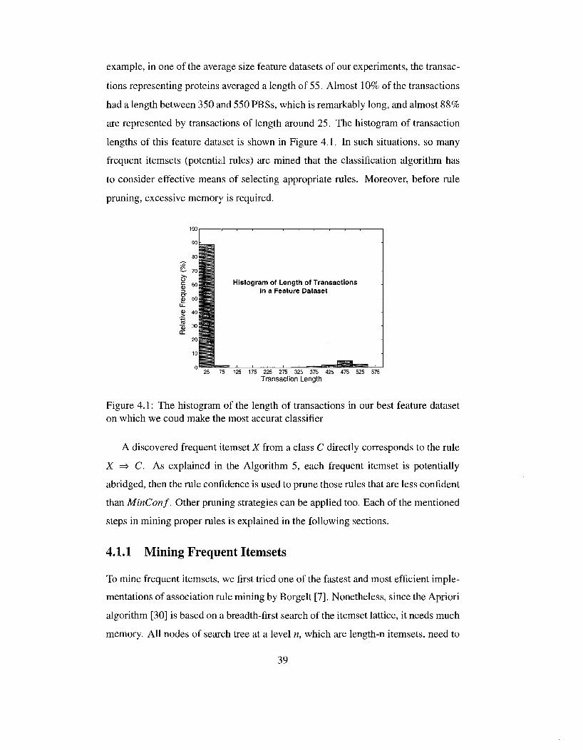
example, in one of the average size feature datasets of our experiments, the transac
tions representing proteins averaged a length of 55. Almost 10% of the transactions
had a length between 350 and 550 PBSs, which is remarkably long, and almost 88%
are represented by transactions of length around 25. The histogram of transaction
lengths of this feature dataset is shown in Figure 4.1. In such situations, so many
frequent itemsets (potential rules) are mined that the classification algorithm has
to consider effective means of selecting appropriate rules. Moreover, before rule
pruning, excessive memory is required.
Histogram of Length of Transactions in a Feature Dataset
25 75 125 175 225 275 325 375 425 475 525 575
Transaction Length
Figure 4.1: The histogram of the length of transactions in our best feature dataset on which we coud make the most accurat classifier
A discovered frequent itemset X from a class C directly corresponds to the rule
X => C. As explained in the Algorithm 5, each frequent itemset is potentially
abridged, then the rule confidence is used to prune those rules that are less confident
than MinConf. Other pruning strategies can be applied too. Each of the mentioned
steps in mining proper rules is explained in the following sections.
4.1.1 Mining Frequent Itemsets
To mine frequent itemsets, we first tried one of the fastest and most efficient imple
mentations of association rule mining by Borgelt [7]. Nonetheless, since the Apriori
algorithm [30] is based on a breadth-first search of the itemset lattice, it needs much
memory. All nodes of search tree at a level n, which are length-n itemsets, need to
39
(D
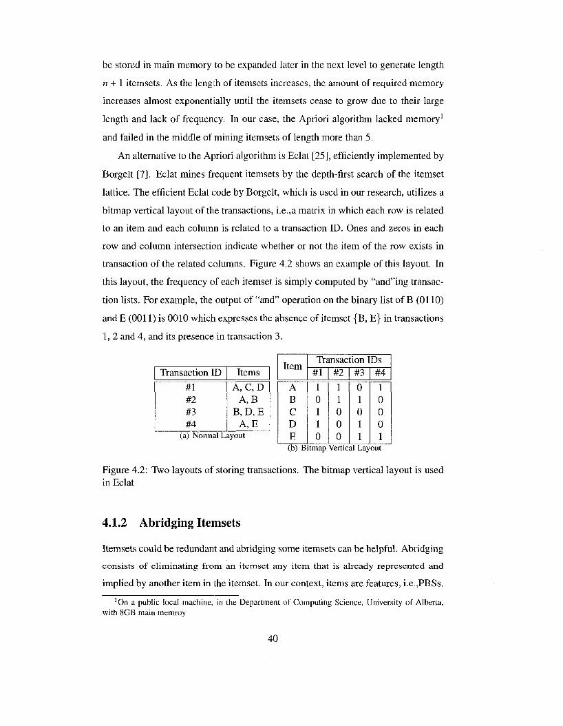
be stored in main memory to be expanded later in the next level to generate length
n + 1 itemsets. As the length of itemsets increases, the amount of required memory
increases almost exponentially until the itemsets cease to grow due to their large
length and lack of frequency. In our case, the Apriori algorithm lacked memory1
and failed in the middle of mining itemsets of length more than 5.
An alternative to the Apriori algorithm is Eclat [25], efficiently implemented by
Borgelt [7]. Eclat mines frequent itemsets by the depth-first search of the itemset
lattice. The efficient Eclat code by Borgelt, which is used in our research, utilizes a
bitmap vertical layout of the transactions, i.e.,a matrix in which each row is related
to an item and each column is related to a transaction ID. Ones and zeros in each
row and column intersection indicate whether or not the item of the row exists in
transaction of the related columns. Figure 4.2 shows an example of this layout. In
this layout, the frequency of each itemset is simply computed by "and"ing transac
tion lists. For example, the output of "and" operation on the binary list of B (0110)
and E (0011) is 0010 which expresses the absence of itemset {B, E} in transactions
1, 2 and 4, and its presence in transaction 3.
Item
A B C D E
Transaction IDs #1
1 0 1 1 0
#2
1 1 0 0 0
#3
0 1 0 1 1
#4
1 0 0 0 1
(b) Bitmap Vertical Layout
Transaction ID
#1 #2 #3 #4
Items
A, C,D A,B
B,D,E A, E
Figure 4.2: Two layouts of storing transactions. The bitmap vertical layout is used in Eclat
4.1.2 Abridging Itemsets
Itemsets could be redundant and abridging some itemsets can be helpful. Abridging
consists of eliminating from an itemset any item that is already represented and
implied by another item in the itemset. In our context, items are features, i.e.,PBSs.
'On a public local machine, in the Department of Computing Science, University of Alberta, with 8GB main memroy
40
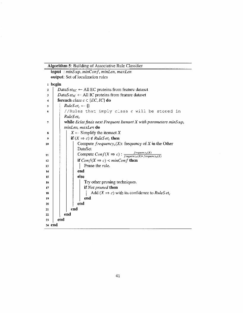
Algorithm 5: Building of Associative Rule Classifier input : minS up, minConf, minLen, maxLen output: Set of localization rules
begin DataS etgc <- All EiC proteins from feature dataset DataS et[c <— All IC proteins from feature dataset foreach class c e {EC, IC} do
RuleSetc <— {} //Rules that imply class c will be stored in RuleS etc
while Eclat finds next Frequent Itemset X with parameters minS up, minLen, maxLen do
X <— Simplify the itemset X if (X => c) $. RuleSetc then
Compute frequency0{X): frequency of X in the Other DataSet
frequency C(X) r J v f frequencyc(X)+frequency0(X)
if Conf(X => c) < minConf then I Prune the rule.
end else
Try other pruning techniques. \i Not pruned then | Add (X => c) with its confidence to RuleS etc
end end
end end
end 24 end
41
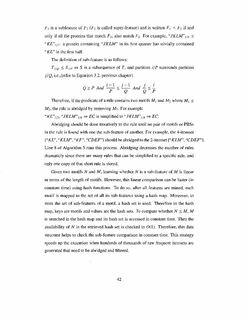
F\ is a subfeature of F2 (F2 is called super-feature) and is written F\ < F2 if and
only if all the proteins that match Fi, also match F2. For example, iiJKLM"i/4 <
"KL"\/2: a protein containing "JKLM" in its first quarter has trivially contained
"KL" in the first half.
The definition of sub-feature is as follows:
Tj/Q < Si/p <=> S is a subsequence of T, arid partition i/P surrounds partition
HQ, i.e.,(refer to Equation 3.2, previous chapter)
i—\ /—l i i 0>P And < - And —<-
P Q Q P
Therefore, if the predicate of a rule contains two motifs M\ and M2 where M\ <
M2, the rule is abridged by removing M2. For example
"KL"U2, "JKLM"U4 => EC is simplified to "JKLM"U4 =̂> EC.
Abridging should be done iteratively to the rule until no pair of motifs or PBSs
in the rule is found with one the sub-feature of another. For example, the 4-itemset
{"KL", "KLM", "EF", "CDEF"} should be abridged to the 2-itemset {"KLM", "CDEF"}.
Line 8 of Algorithm 5 runs this process. Abridging decreases the number of rules
dramaticly since there are many rules that can be simplified to a specific rule, and
only one copy of that short rule is stored.
Given two motifs TV and M, learning whether TV" is a sub-feature of M is linear
in terms of the length of motifs. However, this linear comparison can be faster (in
constant time) using hash functions. To do so, after all features are mined, each
motif is mapped to the set of all its sub-features using a hash map. Moreover, to
store the set of sub-features of a motif, a hash set is used. Therefore in the hash
map, keys are motifs and values are the hash sets. To compare whether N < M, M
is searched in the hash map and its hash set is accessed in constant time. Then the
availability of N in the retrieved hash set is checked in 0(1). Therefore, this data
structure helps to check the sub-feature comparison in constant time. This strategy
speeds up the execution when hundreds of thousands of raw frequent itemsets are
generated that need to be abridged and filtered.
42
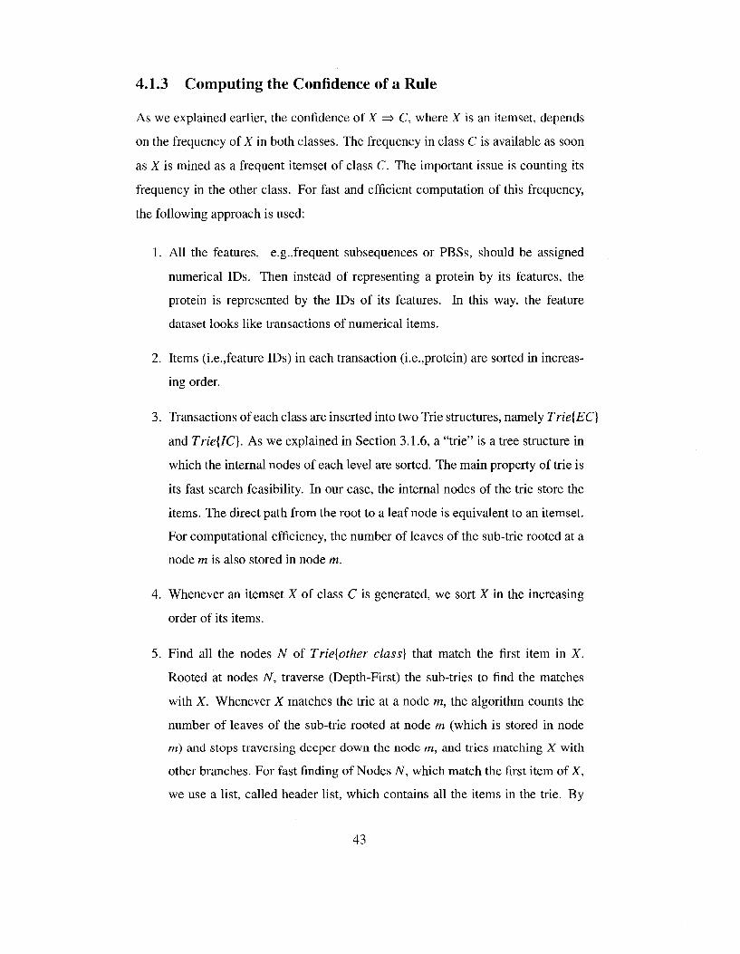
4.1.3 Computing the Confidence of a Rule
As we explained earlier, the confidence of X => C, where X is an itemset, depends
on the frequency of X in both classes. The frequency in class C is available as soon
as X is mined as a frequent itemset of class C. The important issue is counting its
frequency in the other class. For fast and efficient computation of this frequency,
the following approach is used:
1. All the features, e.g.,frequent subsequences or PBSs, should be assigned
numerical IDs. Then instead of representing a protein by its features, the
protein is represented by the IDs of its features. In this way, the feature
dataset looks like transactions of numerical items.
2. Items (i.e.,feature IDs) in each transaction (i.e.,protein) are sorted in increas
ing order.
3. Transactions of each class are inserted into two Trie structures, namely Trie{EC}
and TrietfC}. As we explained in Section 3.1.6, a "trie" is a tree structure in
which the internal nodes of each level are sorted. The main property of trie is
its fast search feasibility. In our case, the internal nodes of the trie store the
items. The direct path from the root to a leaf node is equivalent to an itemset.
For computational efficiency, the number of leaves of the sub-trie rooted at a
node m is also stored in node m.
4. Whenever an itemset X of class C is generated, we sort X in the increasing
order of its items.
5. Find all the nodes N of Trie{other class] that match the first item in X.
Rooted at nodes N, traverse (Depth-First) the sub-tries to find the matches
with X. Whenever X matches the trie at a node m, the algorithm counts the
number of leaves of the sub-trie rooted at node m (which is stored in node
rri) and stops traversing deeper down the node m, and tries matching X with
other branches. For fast finding of Nodes N, which match the first item of X,
we use a list, called header list, which contains all the items in the trie. By
43
following the pointers from an item / in the header list, we can find all the
occurrences (matches) of item / in the trie. Making these pointers is simply
done when the trie is being constructed.
Localization IC IC IC IC IC IC
Transaction 1,2 1,3 3,4
3,4,5,6 3,4,5,7
3,5 (a) Feature dataset of IC proteins
Hea
der
Lis
t
1
2
J
4
5
6
7
(b) Trie(IC}
Figure 4.3: The Trie representation of IC protein transactions
Figure 4.3 shows how a trie represents IC transactions {Trie{IC}). Suppose
X = {3,5} is a frequent itemset of EC proteins. To obtain the frequency of X among
IC proteins, the two nodes of Trie{IC} containing the value 3 are identified first.
Of those two nodes, the leftmost one cannot make a match, but the other node can
make two matches at the nodes containing value 5. One of those two nodes with
value of 5 has 2 leaves in its downward sub-trie and the other one has just 1 leaf.
Therefore, the total occurrence of X in Trie{IC} is three, and now the confidence of
{3,5} => EC can be easily computed.
4.1.4 Pruning the Rules
The minimum confidence requirement (minConf) prunes many rules and lets only
confident rules remain. However, the number of confident rules is still large and
some other pruning techniques are required, as line 16 of Algorithm 5 suggests.
These techniques are as follows:
1. If the confidence of a rule, X => c, reaches 100%, any expansion of its predi
cate results in a rule with 100% confidence too, i.e.,IU Y => c, conf = 100%,
44
where X and Y are two disjoint itemsets and c is a class label. The reason is
clear: all proteins matching the second rule, can also match the first rule, and
the first rule 100% guarantees them to be in class c. In this case, keeping the
first rule suffices, and any other expanded rule is not useful. This technique
prunes many rules especially in Eclat with the depth-first search of the item-
set lattice, because expansion of a rule falls in the deeper levels of lattice, and
Eclat can stop going deeper in the recursion path as soon as it finds a 100%
confident rule.
2. If R is a rule with confidence conf, all the sub-rules of R with confidence less
than conf should be pruned. Ri is a sub-rule of R2 (R2 is called super-rule)
and is written Rr c R2 if and only if any protein that matches R\ can also
match R2 (i.e.,/?2 is more general), further, Ri and R2 should imply the same
class. In other words if Ri is:
n\,n2,... rii =» C with conf = a
and R2 is:
m\,m2,...nij => C with conf = /?
Then Rx E R2 if and only if:
(a) i > j , i.e.,the length of a sub-rule can not be less than that of its super-
rule.
(b) For each item nib (I <b < j), there must be an item na (1 < a < i) such
that na < nib. i.e.,at least one sub-feature of each nib must be found in
the sub-rule.
If a < /3 then R2 is much worth keeping as a more general rule than R\, and
7?i should be removed. In this case, R\ is called the removable sub-rule of R2.
For example suppose 7?i is:
"JKLM"2/4,'TQRST"4/5 =$ EC with conf = 60%
and R2 is:
"KL"i,2 => EC with conf = 90%
45
Rx should be removed and R2 kept because "JKLM"2/4 < "KL"l/2.
When a new rule is to be added in a rule set, this rule has to be compared to
all the older rules. Any older rule that is a removable sub-rule of the new rule, is
removed. If the new rule is a removable sub-rule of any older rule then it is not
added to the set. The data structure used for this rule set is also a Trie similar to
Figure 4.3.
4.2 Evaluating Associative Rule Classifier (Testing Phase)
Given an unknown protein P, a rule can match P when the antecedent of the rule
applies for the features representing P. The rules that match P localize the protein
as EC or IC. To decide between the two classes, there are different possibilities. One
option is to find the rule with the highest confidence, and the predicted class of the
test protein is the class of that rule. There is a drawback to this selection: the effect
of other rules is ignored. For example consider Figure 4.4. Although the first rule
indicates that 90% of proteins that contain feature 1 are IC, the association of 1 with
2, 3, 4 or 5 is something that happens in EC proteins in more than 80% of the cases
(based on the EC rules), which is exactly what is seen in the test protein. Hence, it is
more reasonable to classify the protein as EC rather than IC. Nonetheless, with the
most confident rule, a different classification is made. As an alternative, the average
confidence of the matching rules of each class can be considered. The class with
the highest average of confidences is assigned to P. There is an exceptional case
for which confidence averaging is not used. Whenever a rule with 100% confidence
matches the test protein P, the class label of that rule is assigned to P as long as there
is no other 100% confident rule of the other class. The reason is that 100% confident
rules exhibit unique facts (derived from the training samples) about proteins of a
class that is never met in the proteins of the other class.
In a few cases, a test protein cannot match any rule from any class. Moreover,
there are cases that a test protein is equally classified as both EC and IC. The latter
happens mainly when there are EC and IC rules with 100% confidence, and both
can match and classify the test protein, or when the confidence averages are the
46
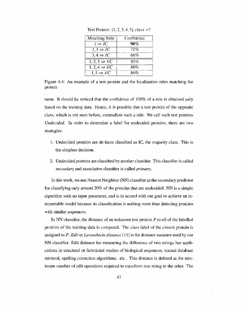
Test Protein: {1,2,3,4,5}, class =?
Matching Rule 1 =>/C
2,3 => IC 3,4=>/C
1,2,3 =>EC 1,2,4 => EC 1,5=>£C
Confidence 90% 71% 68%
85% 88% 86%
Figure 4.4: An example of a test protein and the localization rules matching the protein
same. It should be noticed that the confidence of 100% of a rule is obtained only
based on the training data. Hence, it is possible that a test protein of the opposite
class, which is not seen before, contradicts such a rule. We call such test proteins
Undecided. In order to determine a label for undecided proteins, there are two
strategies:
1. Undecided proteins are de-facto classified as IC, the majority class. This is
the simplest decision.
2. Undecided proteins are classified by another classifier. This classifier is called
secondary and associative classifier is called primary.
In this work, we use Nearest Neighbor (NN) classifier as the secondary predictor
for classifying only around 20% of the proteins that are undecided. NN is a simple
algorithm with no input parameter, and is in accord with our goal to achieve an in-
terpretable model because its classification is nothing more than detecting proteins
with similar sequences.
In NN classifier, the distance of an unknown test protein P to all of the labelled
proteins of the training data is computed. The class label of the closest protein is
assigned to P. Edit or Levenshtein distance [11] is the distance measure used by our
NN classifier. Edit distance for measuring the difference of two strings has appli
cations in structural or functional studies of biological sequences, textual database
retrieval, spelling correction algorithms, etc . This distance is defined as the min
imum number of edit operations required to transform one string to the other. The
47
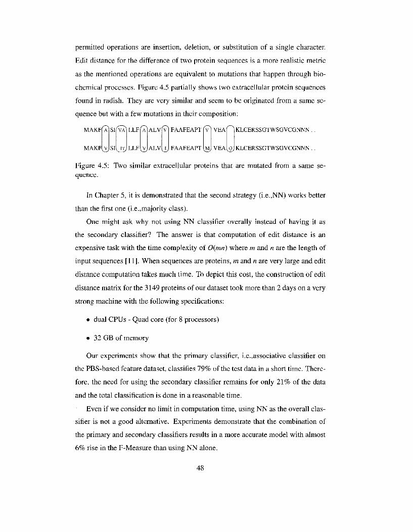
permitted operations are insertion, deletion, or substitution of a single character.
Edit distance for the difference of two protein sequences is a more realistic metric
as the mentioned operations are equivalent to mutations that happen through bio
chemical processes. Figure 4.5 partially shows two extracellular protein sequences
found in radish. They are very similar and seem to be originated from a same se
quence but with a few mutations in their composition:
MAKF A SIf VAl LLF A ALV V FAAFEAPT V VEA r^ KLCERSSGTWSGVCGNNN.
M AKF ^VJS I^JTJ LLF^vjALVl^ FAAFEAPT \M) VEA[ojKLCERSSGTWSGVCGNNN ..
Figure 4.5: Two similar extracellular proteins that are mutated from a same sequence.
In Chapter 5, it is demonstrated that the second strategy (i.e.,NN) works better
than the first one (i.e.,majority class).
One might ask why not using NN classifier overally instead of having it as
the secondary classifier? The answer is that computation of edit distance is an
expensive task with the time complexity of 0(mn) where m and n are the length of
input sequences [11]. When sequences are proteins, m and n are very large and edit
distance computation takes much time. To depict this cost, the construction of edit
distance matrix for the 3149 proteins of our dataset took more than 2 days on a very
strong machine with the following specifications:
• dual CPUs - Quad core (for 8 processors)
• 32 GB of memory
Our experiments show that the primary classifier, i.e.,associative classifier on
the PBS-based feature dataset, classifies 79% of the test data in a short time. There
fore, the need for using the secondary classifier remains for only 21% of the data
and the total classification is done in a reasonable time.
Even if we consider no limit in computation time, using NN as the overall clas
sifier is not a good alternative. Experiments demonstrate that the combination of
the primary and secondary classifiers results in a more accurate model with almost
6% rise in the F-Measure than using NN alone.
48
Chapter 5
Experimental Results
In this chapter, we evaluate our models for predicting subcellular localization and
demonstrate the discriminative power of partition-based subsequences. The main
classification algorithm that has been the focus of this work is the associative clas
sifier. However, because of the growing interest in SVM and its strong ability to
classify high dimensional data, we compare our results with those of SVM. Deci
sion tree classifiers, generating a human readable and interpretable model, are also
studied.
5.1 Dataset and Evaluation Methodology
We performed our method on a plant protein dataset from the Proteome Analyst
Project [46] at the University of Alberta. The dataset is constructed from SWISS-
PROT. After cleaning the data, i.e.,removing repetitive or defective proteins which
contain nonexistent amino acids, 3,149 proteins remained. The portion of EC pro
teins is only 4% of the data which shows the severe imbalance in the data.
To evaluate the performance of classifiers, Overall Accuracy is often used.
However, this is usually inappropriate particularly with imbalanced data. In our
case with 96% of proteins being IC, a classifier that always classifies as IC achieves
the overall accuracy of 96% while no EC proteins are correctly classified. Instead,
we chose precision, recall and F-measure with respect to EC (i.e.,the target class).
These three measures are commonly used in this field of research. Using them in
our work allows easier comparison with the related approaches. We did not choose
49
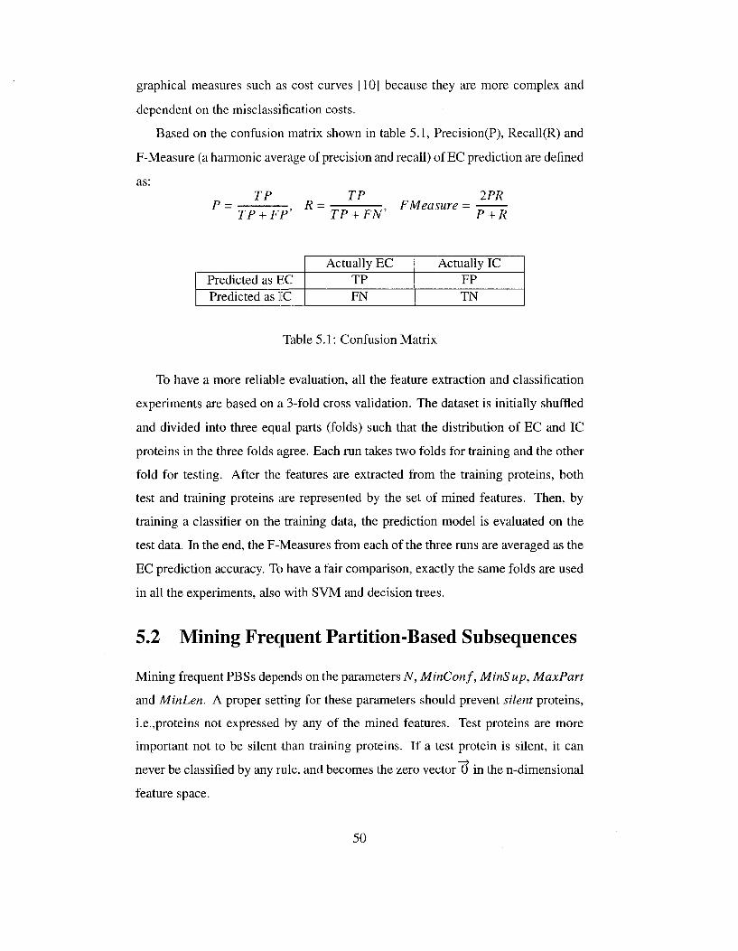
graphical measures such as cost curves [10] because they are more complex and
dependent on the misclassification costs.
Based on the confusion matrix shown in table 5.1, Precision(P), Recall(R) and
F-Measure (a harmonic average of precision and recall) of EC prediction are defined
as:
P = TP
TP + FP' R =
TP TP + FN'
F Measure = 2PR
P + R
Predicted as EC Predicted as IC
Actually EC TP FN
Actually IC FP TN
Table 5.1: Confusion Matrix
To have a more reliable evaluation, all the feature extraction and classification
experiments are based on a 3-fold cross validation. The dataset is initially shuffled
and divided into three equal parts (folds) such that the distribution of EC and IC
proteins in the three folds agree. Each run takes two folds for training and the other
fold for testing. After the features are extracted from the training proteins, both
test and training proteins are represented by the set of mined features. Then, by
training a classifier on the training data, the prediction model is evaluated on the
test data. In the end, the F-Measures from each of the three runs are averaged as the
EC prediction accuracy. To have a fair comparison, exactly the same folds are used
in all the experiments, also with SVM and decision trees.
5.2 Mining Frequent Partition-Based Subsequences
Mining frequent PBSs depends on the parameters N, MinConf, MinS up, MaxPart
and MinLen. A proper setting for these parameters should prevent silent proteins,
i.e.,proteins not expressed by any of the mined features. Test proteins are more
important not to be silent than training proteins. If a test protein is silent, it can
never be classified by any rule, and becomes the zero vector 0 in the n-dimensional
feature space.
50
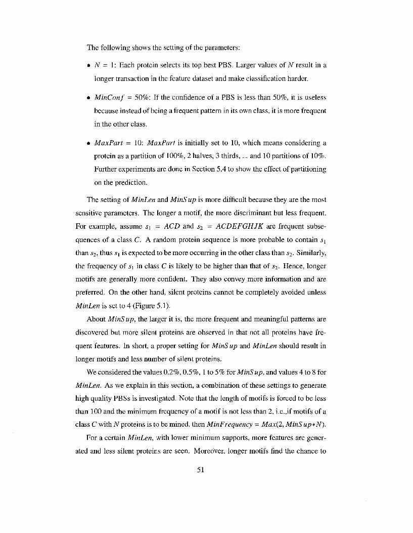
The following shows the setting of the parameters:
• TV = 1: Each protein selects its top best PBS. Larger values of N result in a
longer transaction in the feature dataset and make classification harder.
• MinConf = 50%: If the confidence of a PBS is less than 50%, it is useless
because instead of being a frequent pattern in its own class, it is more frequent
in the other class.
• MaxPart = 10: MaxPart is initially set to 10, which means considering a
protein as a partition of 100%, 2 halves, 3 thirds,... and 10 partitions of 10%.
Further experiments are done in Section 5.4 to show the effect of partitioning
on the prediction.
The setting of MinLen and MinS up is more difficult because they are the most
sensitive parameters. The longer a motif, the more discriminant but less frequent.
For example, assume si -= ACD and s2 = ACDEFGHJK are frequent subse
quences of a class C. A random protein sequence is more probable to contain s\
than s2, thus ^i is expected to be more occurring in the other class than s2. Similarly,
the frequency of s\ in class C is likely to be higher than that of s2. Hence, longer
motifs are generally more confident. They also convey more information and are
preferred. On the other hand, silent proteins cannot be completely avoided unless
MinLen is set to 4 (Figure 5.1).
About MinS up, the larger it is, the more frequent and meaningful patterns are
discovered but more silent proteins are observed in that not all proteins have fre
quent features. In short, a proper setting for MinS up and MinLen should result in
longer motifs and less number of silent proteins.
We considered the values 0.2%, 0.5%, 1 to 5% for MinS up, and values 4 to 8 for
MinLen. As we explain in this section, a combination of these settings to generate
high quality PBSs is investigated. Note that the length of motifs is forced to be less
than 100 and the minimum frequency of a motif is not less than 2, i.e.,if motifs of a
class C with N proteins is to be mined, then MinFrequency = Max(2, MinS up*N).
For a certain MinLen, with lower minimum supports, more features are gener
ated and less silent proteins are seen. Moreover, longer motifs find the chance to
51
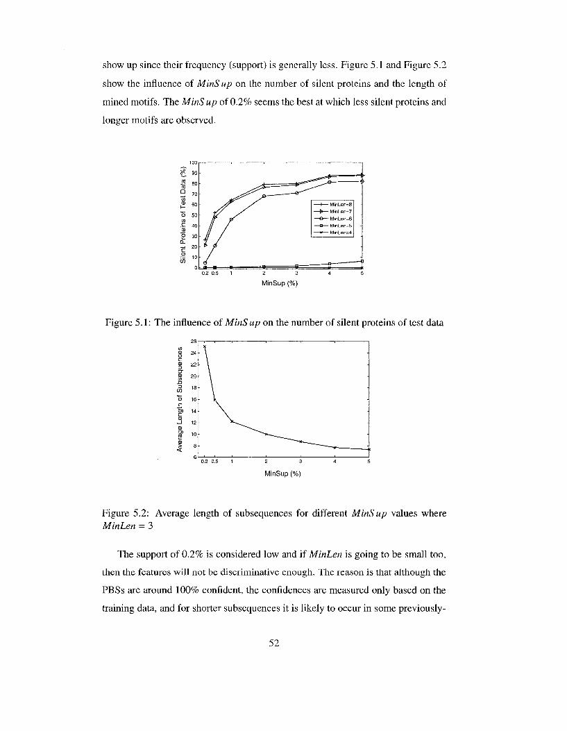
show up since their frequency (support) is generally less. Figure 5.1 and Figure 5.2
show the influence of MinSup on the number of silent proteins and the length of
mined motifs. The MinS up of 0.2% seems the best at which less silent proteins and
longer motifs are observed.
2 3
MinSup (%)
Figure 5.1: The influence of MinS up on the number of silent proteins of test data
5> 22
Figure 5.2: Average length of subsequences for different MinSup values where MinLen = 3
The support of 0.2% is considered low and if MinLen is going to be small too,
then the features will not be discriminative enough. The reason is that although the
PBSs are around 100% confident, the confidences are measured only based on the
training data, and for shorter subsequences it is likely to occur in some previously-
52
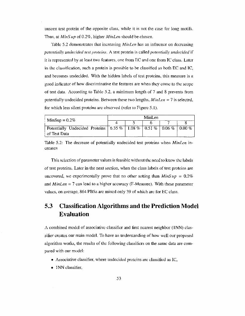
unseen test protein of the opposite class, while it is not the case for long motifs.
Thus, at MinSup of 0.2%, higher MinLen should be chosen.
Table 5.2 demonstrates that increasing MinLen has an influence on decreasing
potentially undecided test proteins. A test protein is called potentially undecided if
it is represented by at least two features, one from EC and one from IC class. Later
in the classification, such a protein is possible to be classified as both EC and IC,
and becomes undecided. With the hidden labels of test proteins, this measure is a
good indicator of how discriminative the features are when they come to the scope
of test data. According to Table 5.2, a minimum length of 7 and 8 prevents from
potentially undecided proteins. Between these two lengths, MinLen = 7 is selected,
for which less silent proteins are observed (refer to Figure 5.1).
MinSup = 0.2%
Potentially Undecided Proteins of Test Data
MinLen 4
6.35 % 5
1.08% 6
0.51 % 7
0.06 % 8
0.00 %
Table 5.2: The decrease of potentially undecided test proteins when MinLen increases
This selection of parameter values is feasible without the need to know the labels
of test proteins. Later in the next section, when the class labels of test proteins are
uncovered, we experimentally prove that no other setting than MinSup = 0.2%
and MinLen - 7 can lead to a higher accuracy (F-Measure). With these parameter
values, on average, 864 PBSs are mined only 39 of which are for EC class.
5.3 Classification Algorithms and the Prediction Model Evaluation
A combined model of associative classifier and first nearest neighbor (INN) clas
sifier creates our main model. To have an understanding of how well our proposed
algorithm works, the results of the following classifiers on the same data are com
pared with our model:
• Associative classifier, where undecided proteins are classified as IC,
• INN classifier,
53
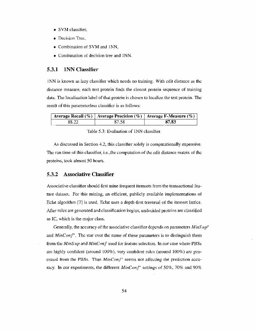
• SVM classifier,
• Decision Tree,
• Combination of SVM and INN,
• Combination of decision tree and INN.
5.3.1 INN Classifier
INN is known as lazy classifier which needs no training. With edit distance as the
distance measure, each test protein finds the closest protein sequence of training
data. The localization label of that protein is chosen to localize the test protein. The
result of this parameterless classifier is as follows:
Average Recall (%) 88.22
Average Precision (%) 87.58
Average F-Measure (%) 87.83
Table 5.3: Evaluation of INN classifier.
As discussed in Section 4.2, this classifier solely is computationally expensive.
The run time of this classifier, i.e.,the computation of the edit distance matrix of the
proteins, took almost 50 hours.
5.3.2 Associative Classifier
Associative classifier should first mine frequent itemsets from the transactional fea
ture dataset. For this mining, an efficient, publicly available implementations of
Eclat algorithm [7] is used. Eclat uses a depth-first traversal of the itemset lattice.
After rules are generated and classification begins, undecided proteins are classified
as IC, which is the major class.
Generally, the accuracy of the associative classifier depends on parameters MinS up*
and MinConf*. The star over the name of these parameters is to distinguish them
from the MinS up and MinConf used for feature selection. In our case where PBSs
are highly confident (around 100%), very confident rules (around 100%) are gen
erated from the PBSs. Thus MinConf* seems not affecting the prediction accu
racy. In our experiments, the different MinConf* settings of 50%, 70% and 90%
54
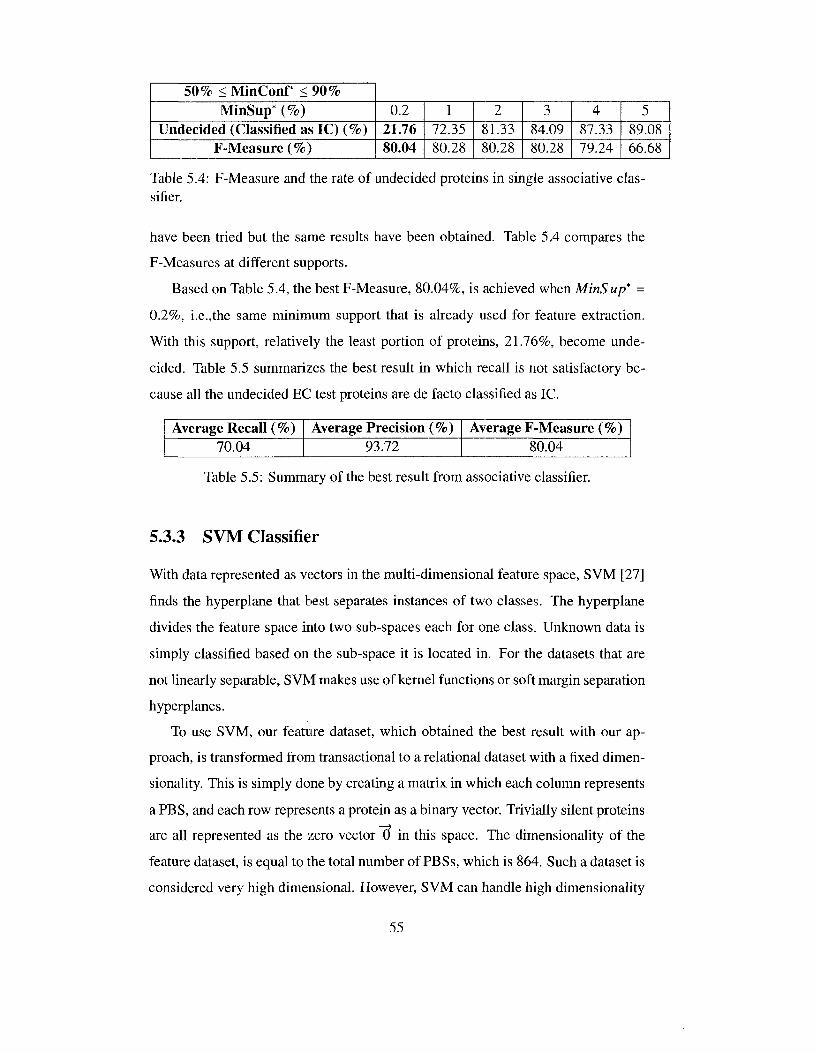
50% < MinConf < 90% MinSup* (%)
Undecided (Classified as IC) (%) F-Measure (%)
0.2 21.76 80.04
1 72.35 80.28
2 81.33 80.28
3 84.09 80.28
4 87.33 79.24
5 89.08 66.68
Table 5.4: F-Measure and the rate of undecided proteins in single associative classifier.
have been tried but the same results have been obtained. Table 5.4 compares the
F-Measures at different supports.
Based on Table 5.4, the best F-Measure, 80.04%, is achieved when MinSup* =
0.2%, i.e.,the same minimum support that is already used for feature extraction.
With this support, relatively the least portion of proteins, 21.76%, become unde
cided. Table 5.5 summarizes the best result in which recall is not satisfactory be
cause all the undecided EC test proteins are de facto classified as IC.
Average Recall (%) 70.04
Average Precision (%) 93.72
Average F-Measure (%) 80.04
Table 5.5: Summary of the best result from associative classifier.
5.3.3 SVM Classifier
With data represented as vectors in the multi-dimensional feature space, SVM [27]
finds the hyperplane that best separates instances of two classes. The hyperplane
divides the feature space into two sub-spaces each for one class. Unknown data is
simply classified based on the sub-space it is located in. For the datasets that are
not linearly separable, SVM makes use of kernel functions or soft margin separation
hyperplanes.
To use SVM, our feature dataset, which obtained the best result with our ap
proach, is transformed from transactional to a relational dataset with a fixed dimen
sionality. This is simply done by creating a matrix in which each column represents
a PBS, and each row represents a protein as a binary vector. Trivially silent proteins
are all represented as the zero vector 0 in this space. The dimensionality of the
feature dataset, is equal to the total number of PBSs, which is 864. Such a dataset is
considered very high dimensional. However, SVM can handle high dimensionality
55
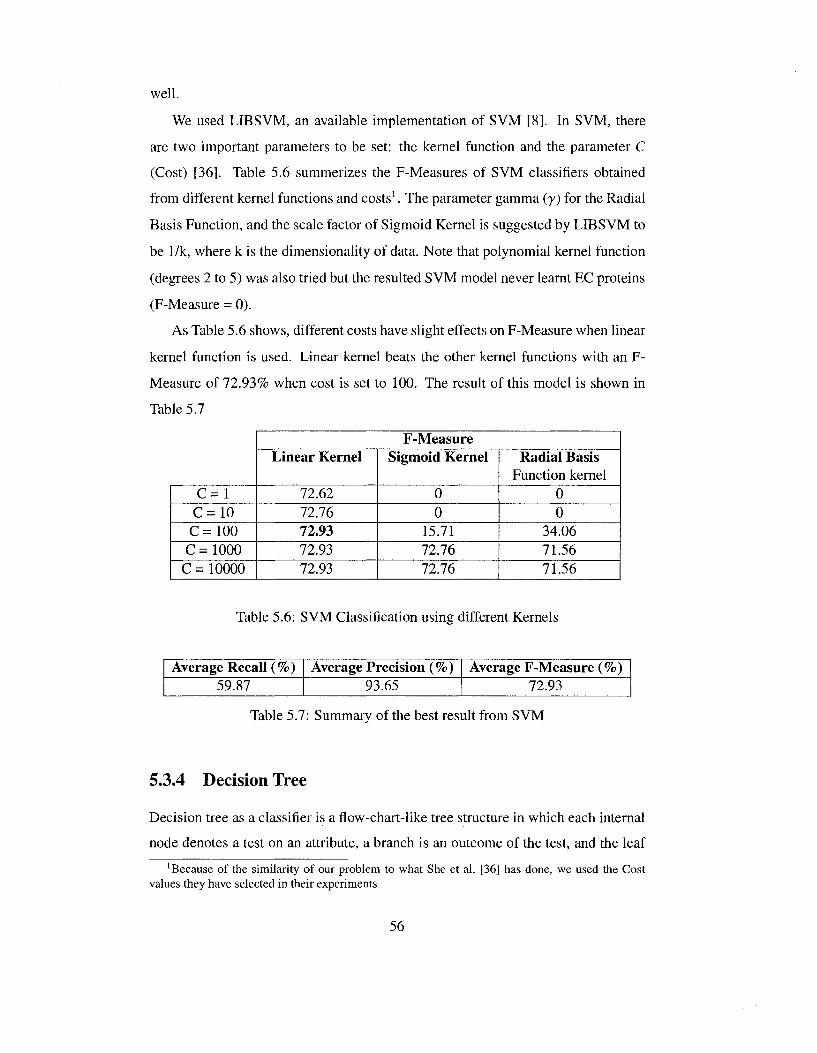
well.
We used LIBSVM, an available implementation of SVM [8]. In SVM, there
are two important parameters to be set: the kernel function and the parameter C
(Cost) [36]. Table 5.6 summerizes the F-Measures of SVM classifiers obtained
from different kernel functions and costs1. The parameter gamma (y) for the Radial
Basis Function, and the scale factor of Sigmoid Kernel is suggested by LIBSVM to
be 1/k, where k is the dimensionality of data. Note that polynomial kernel function
(degrees 2 to 5) was also tried but the resulted SVM model never learnt EC proteins
(F-Measure = 0).
As Table 5.6 shows, different costs have slight effects on F-Measure when linear
kernel function is used. Linear kernel beats the other kernel functions with an F-
Measure of 72.93% when cost is set to 100. The result of this model is shown in
Table 5.7
C = l C = 1 0
C=100 C = 1000
C = 10000
F-Measure Linear Kernel
72.62 72.76 72.93 72.93 72.93
Sigmoid Kernel
0 0
15.71 72.76 72.76
Radial Basis Function kernel
0 0
34.06 71.56 71.56
Table 5.6: SVM Classification using different Kernels
Average Recall (%) 59.87
Average Precision (%) 93.65
Average F-Measure (%) 72.93
Table 5.7: Summary of the best result from SVM
5.3.4 Decision Tree
Decision tree as a classifier is a flow-chart-like tree structure in which each internal
node denotes a test on an attribute, a branch is an outcome of the test, and the leaf
'Because of the similarity of our problem to what She et al. [36] has done, we used the Cost values they have selected in their experiments
56
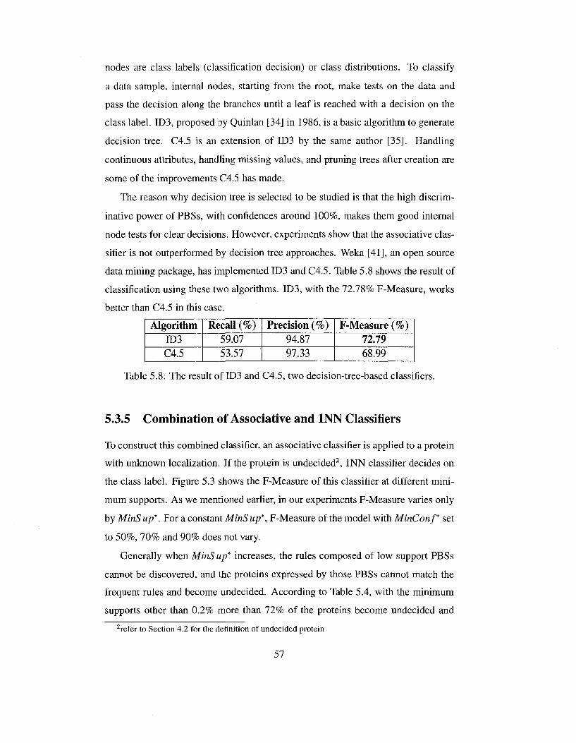
nodes are class labels (classification decision) or class distributions. To classify
a data sample, internal nodes, starting from the root, make tests on the data and
pass the decision along the branches until a leaf is reached with a decision on the
class label. ID3, proposed by Quinlan [34] in 1986, is a basic algorithm to generate
decision tree. C4.5 is an extension Of ID3 by the same author [35]. Handling
continuous attributes, handling missing values, and pruning trees after creation are
some of the improvements C4.5 has made.
The reason why decision tree is selected to be studied is that the high discrim
inative power of PBSs, with confidences around 100%, makes them good internal
node tests for clear decisions. However, experiments show that the associative clas
sifier is not outperformed by decision tree approaches. Weka [41], an open source
data mining package, has implemented ID3 and C4.5. Table 5.8 shows the result of
classification using these two algorithms. ID3, with the 72.78% F-Measure, works
better than C4.5 in this case.
Algorithm ID3 C4.5
Recall (%) 59.07 53.57
Precision (%) 94.87 97.33
F-Measure (%) 72.79 68.99
Table 5.8: The result of ID3 and C4.5, two decision-tree-based classifiers.
5.3.5 Combination of Associative and INN Classifiers
To construct this combined classifier, an associative classifier is applied to a protein
with unknown localization. If the protein is undecided2, INN classifier decides on
the class label. Figure 5.3 shows the F-Measure of this classifier at different mini
mum supports. As we mentioned earlier, in our experiments F-Measure varies only
by MinS up*. For a constant MinS up*, F-Measure of the model with MinConf* set
to 50%, 70% and 90% does not vary.
Generally when MinS up* increases, the rules composed of low support PBSs
cannot be discovered, and the proteins expressed by those PBSs cannot match the
frequent rules and become undecided. According to Table 5.4, with the minimum
supports other than 0.2% more than 72% of the proteins become undecided and
2refer to Section 4.2 for the definition of undecided protein
57
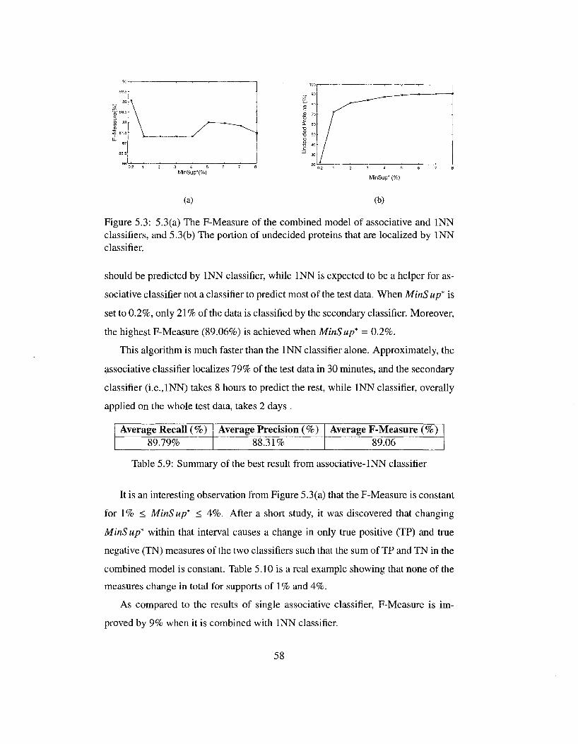
MinSup*(%) MinSup* (%)
(a) (b)
Figure 5.3: 5.3(a) The F-Measure of the combined model of associative and INN classifiers, and 5.3(b) The portion of undecided proteins that are localized by INN classifier.
should be predicted by INN classifier, while INN is expected to be a helper for as
sociative classifier not a classifier to predict most of the test data. When MinS up* is
set to 0.2%, only 21% of the data is classified by the secondary classifier. Moreover,
the highest F-Measure (89.06%) is achieved when MinSup* = 0.2%.
This algorithm is much faster than the INN classifier alone. Approximately, the
associative classifier localizes 79% of the test data in 30 minutes, and the secondary
classifier (i.e.,INN) takes 8 hours to predict the rest, while INN classifier, overally
applied on the whole test data, takes 2 days .
Average Recall (%) 89.79%
Average Precision (%) 88.31%
Average F-Measure (%) 89.06
Table 5.9: Summary of the best result from associative-INN classifier
It is an interesting observation from Figure 5.3(a) that the F-Measure is constant
for 1% < MinSup* < 4%. After a short study, it was discovered that changing
MinS up* within that interval causes a change in only true positive (TP) and true
negative (TN) measures of the two classifiers such that the sum of TP and TN in the
combined model is constant. Table 5.10 is a real example showing that none of the
measures change in total for supports of 1% and 4%.
As compared to the results of single associative classifier, F-Measure is im
proved by 9% when it is combined with INN classifier.
58
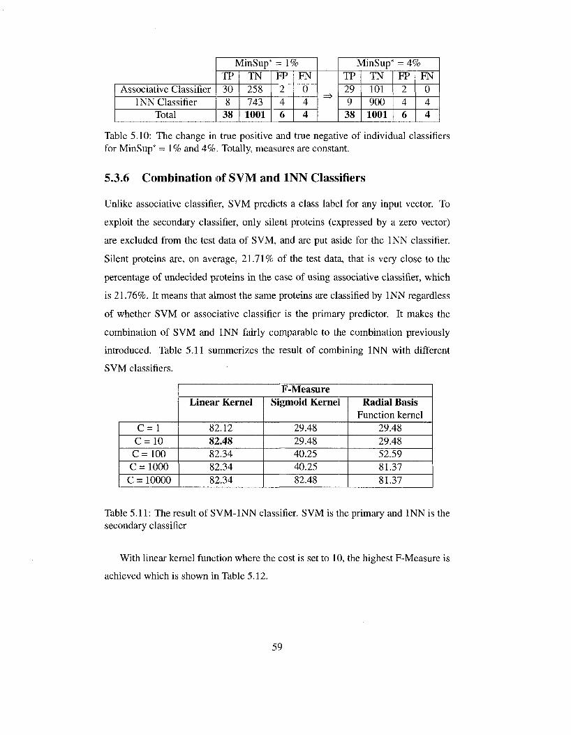
Associative Classifier INN Classifier
Total
MinSup* = 1% TP 30 8
38
TN 258 743 1001
FP 2 4 6
FN 0 4 4
=>
MinSup* = 4% TP 29 9
38
TN 101 900 1001
FP 2 4 6
FN 0 4 4
Table 5.10: The change in true positive and true negative of individual classifiers for MinSup* = 1% and 4%. Totally, measures are constant.
5.3.6 Combination of SVM and INN Classifiers
Unlike associative classifier, SVM predicts a class label for any input vector. To
exploit the secondary classifier, only silent proteins (expressed by a zero vector)
are excluded from the test data of SVM, and are put aside for the INN classifier.
Silent proteins are, on average, 21.71% of the test data, that is very close to the
percentage of undecided proteins in the case of using associative classifier, which
is 21.76%. It means that almost the same proteins are classified by INN regardless
of whether SVM or associative classifier is the primary predictor. It makes the
combination of SVM and INN fairly comparable to the combination previously
introduced. Table 5.11 summerizes the result of combining INN with different
SVM classifiers.
C = l C = 1 0 C=100
C = 1000 C = 10000
F-Measure Linear Kernel
82.12 82.48 82.34 82.34 82.34
Sigmoid Kernel
29.48 29.48 40.25 40.25 82.48
Radial Basis Function kernel
29.48 29.48 52.59 81.37 81.37
Table 5.11: The result of SVM-1NN classifier. SVM is the primary and INN is the secondary classifier
With linear kernel function where the cost is set to 10, the highest F-Measure is
achieved which is shown in Table 5.12.
59
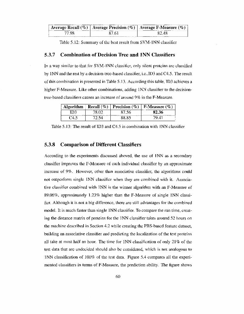
Average Recall (%) 77.98
Average Precision (%) 87.61
Average F-Measure (%) 82.48
Table 5.12: Summary of the best result from SVM-1NN classifier
5.3.7 Combination of Decision Tree and INN Classifiers
In a way similar to that for SVM-1NN classifier, only silent proteins are classified
by INN and the rest by a decision-tree-based classifier, i.e.,ID3 and C4.5. The result
of this combination is presented in Table 5.13. According this table, ID3 achieves a
higher F-Measure. Like other combinations, adding INN classifier to the decision-
tree-based classifiers causes an increase of around 9% in the F-Measure.
Algorithm ID3 C4.5
Recall (%) 78.02 72.54
Precision (%) 87.56 88.85
F-Measure (%) 82.36 79.41
Table 5.13: The result of ID3 and C4.5 in combination with INN classifier
5.3.8 Comparison of Different Classifiers
According to the experiments discussed aboved, the use of INN as a secondary
classifier improves the F-Measure of each individual classifier by an approximate
increase of 9%. However, other than associative classifier, the algorithms could
not outperform single INN classifier when they are combined with it. Associa
tive classifier combined with INN is the winner algorithm with an F-Measure of
89.06%, approximately 1.23% higher than the F-Measure of single INN classi
fier. Although it is not a big difference, there are still advantages for the combined
model. It is much faster than single INN classifier. To compare the run time, creat
ing the distance matrix of proteins for the INN classifier takes around 52 hours on
the machine described in Section 4.2 while creating the PBS-based feature dataset,
building an associative classifier and predicting the localization of the test proteins
all take at most half an hour. The time for INN classification of only 21% of the
test data that are undecided should also be considered, which is not analogous to
INN classification of 100% of the test data. Figure 5.4 compares all the experi
mented classifiers in terms of F-Measure, the prediction ability. The figure shows
60
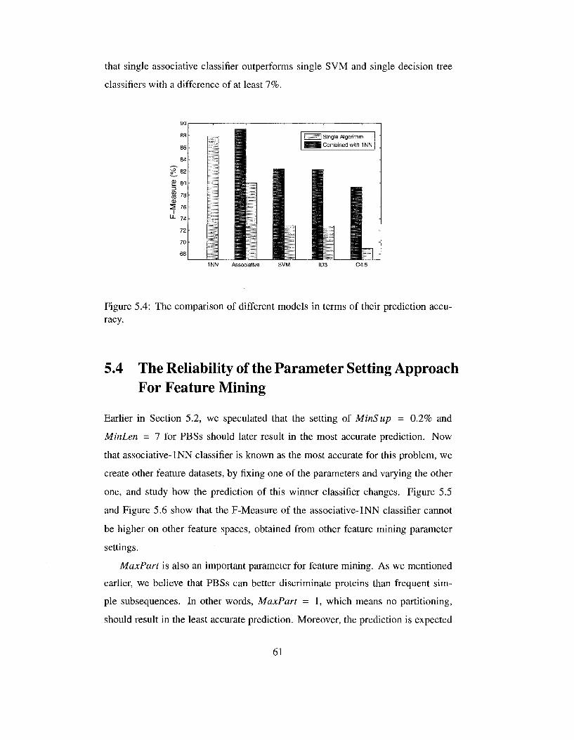
that single associative classifier outperforms single SVM and single decision tree
classifiers with a difference of at least 7%.
90
88
86 •
84
^ 8 2 -
£ 80
CD '8 <D 2 76
I " - 74 -
72
70
I 1
I I Single Algorithm
IHSU! Combined with 1NN
Figure 5.4: The comparison of different models in terms of their prediction accuracy.
5.4 The Reliability of the Parameter Setting Approach For Feature Mining
Earlier in Section 5.2, we speculated that the setting of MinSup = 0.2% and
MinLen = 7 for PBSs should later result in the most accurate prediction. Now
that associative-INN classifier is known as the most accurate for this problem, we
create other feature datasets, by fixing one of the parameters and varying the other
one, and study how the prediction of this winner classifier changes. Figure 5.5
and Figure 5.6 show that the F-Measure of the associative-INN classifier cannot
be higher on other feature spaces, obtained from other feature mining parameter
settings.
MaxPart is also an important parameter for feature mining. As we mentioned
earlier, we believe that PBSs can better discriminate proteins than frequent sim
ple subsequences. In other words, MaxPart = 1, which means no partitioning,
should result in the least accurate prediction. Moreover, the prediction is expected
61
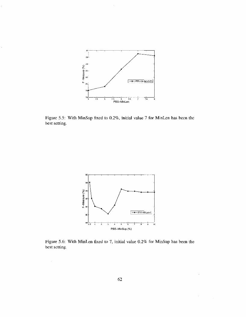
Figure 5.5: With MinSup fixed to 0.2%, initial value 7 for MinLen has been the best setting.
89
Cp" 88
(D
« 87 CO CD
l±_ 86
85
\
^ X / \ / | —•— PBS-MinLsn=71
0.2 1 2 3 4 5 7 8 9 10
PBS-MinSup (%)
Figure 5.6: With MinLen fixed to 7, initial value 0.2% for MinSup has been the best setting.
62
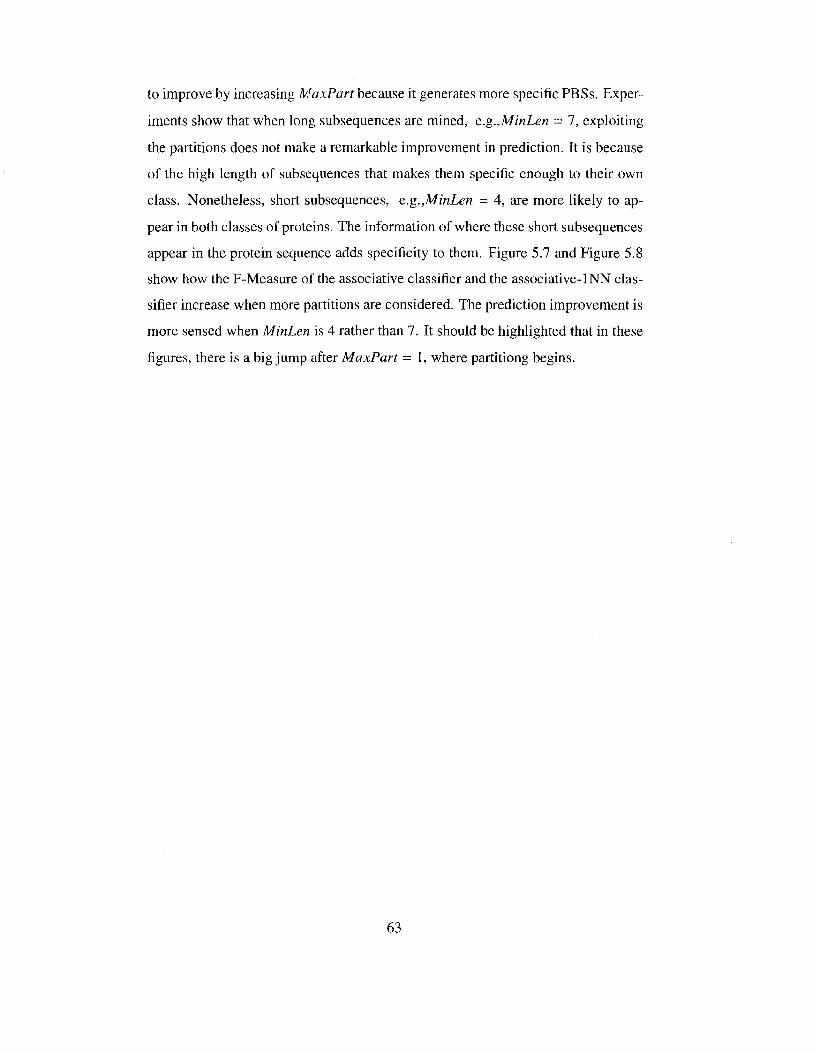
to improve by increasing MaxPart because it generates more specific PBSs. Exper
iments show that when long subsequences are mined, e.g.,MinLen = 7, exploiting
the partitions does not make a remarkable improvement in prediction. It is because
of the high length of subsequences that makes them specific enough to their own
class. Nonetheless, short subsequences, e.g.,MinLen = 4, are more likely to ap
pear in both classes of proteins. The information of where these short subsequences
appear in the protein sequence adds specificity to them. Figure 5.7 and Figure 5.8
show how the F-Measure of the associative classifier and the associative-INN clas
sifier increase when more partitions are considered. The prediction improvement is
more sensed when MinLen is 4 rather than 7. It should be highlighted that in these
figures, there is a big jump after MaxPart = 1, where partitiong begins.
63
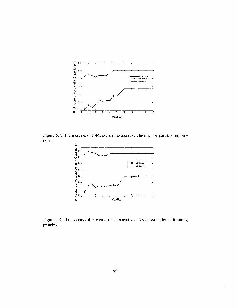
ffl
o <1>
> ra o
78
/ti
- MinLen=7
- Minl_en=4
0 12 14 16 18 20
MaxPart
Figure 5.7: The increase of F-Measure in associative classifier by partitioning proteins.
CD
it: 90 co in CO
O 88
Z Z 86 T
CO
<
5 I
—M »« M H M K —
- Minl_en=7 - MinLen=4
10 12 14 16 18 20 MaxPart
Figure 5.8: The increase of F-Measure in associative-INN classifier by partitioning proteins.
64
Chapter 6
Conclusion And Future Work
In this research, we proposed a new discriminative feature for predicting extracel
lular proteins. Partition-Based Subsequences have a strong ability, higher than sim
ple subsequences, to discriminate between the proteins of different localizations.
Moreover, they seem to encode more information about the structure of proteins by
showing the regions along the protein sequences where special subsequences ap
pear most. We applied an associative classifier on the feature datasets. With some
simple, interpretable and highly confident rules most of proteins are well classified.
In a few cases where an associative classifier is not certain about the localization of
a protein, a nearest neighbor classifier based on edit distance is utilized. The com
bination of the associative and the nearest neighbor classifiers is a strong model to
predict extracellular proteins with an F-Measure of 89.06%, which is significantly
above the state-of-the-art, almost 5% above the F-Measure of Proteome Analyst and
the previous work, which is specifically on EC prediction using the same dataset.
The presicion of this model is 88.31%, and its recall is 89.79%. Our associative
classifier also outperforms SVM and decision tree classifiers such as ID3 and C4.5
on the same feature space with a large difference of at least 7% in the F-Measure.
As one future work, this binary classifier can be extended to a complete local
ization problem. This can be done hierarchically. In the first step, a decision is
made whether a protein is extracellular or intracellular. If it is intracellular, next
steps similarly investigate which intracellular location the protein resides in. In
each step, one location is specifically learnt while the remainder is called "other"
until all the locations are learnt in the end.
65
Another interesting work is to use another alphabet for representing proteins and
extract frequent subsequence-based features in this new representation. There are
biochemical similarities among some of the amino acids []. In this context, two or
more similar amino acids (with similar properties) can be grouped and represented
by a single alphabetic code. It reduces the number of characters in the string rep-
resention of proteins, and may generate smaller but more valuable set of features.
Therefore, instead of chains of amino acids alone, chains of amino acid groups will
be found which might be more meaningful to biologists.
66
Bibliography
[1] National human genome research institute. http://en.wikipedia.Org/wiki/Image:Protein-structure.png.
[2] Bender A., van Dooren G. G., Ralph S. A., McFadden G. I., and Schneider G. Properties and prediction of mitochondrial transit peptides from plasmodium falciparum. Molecular and Biochemical Parasitology, 132(2):59-66, 2003.
[3] Campbell N. A., Reece J. B., Taylor M. R., Simon E. J., and Dickey J. L. Biology : concepts and connections. Pearson Higher Education, 6 edition, 2009.
[4] Hoglund A., Donnes P., Blum T., Adolph H. W., and Kohlbacher O. Mul-tiloc: prediction of protein subcellular localization using n-terminal targeting sequences, sequence motifs and amino acid composition. Bioinformatics, 22(10): 1158-1165, 2006.
[5] Reinhardt A. and Hubbard T. Using neural networks for prediction of the subcellular location of proteins. Nucleic acids research, 26(9):2230-2236, 1998.
[6] Lukas K. B. and Rashidi H. H. Bioinformatics Basics: Applications in Biological Science and Medicine. CRC Taylor and Francis, 2nd edition edition, 2005.
[7] Borgelt C. Efficient implementations of apriori and eclat. In Proceedings of the IEEE ICDM Workshop on Frequent Itemset Mining Implementations (FIMI03), Melbourne, Florida, USA, 2003. software available at http://fuzzy.cs.uni-magdeburg.de/borgelt/software.html.
[8] Chang C. C. and Lin C. J. Libsvm : a library for support vector machines, 2001. software available at http://www.csie.ntu.edu.tw/ cjlin/libsvm.
[9] Chou K. C. and Elrod D. W. Protein subcellular location prediction. Protein Engineering, 12(2): 107-118, 1999.
[10] Drummond C. and Holte R. C. Explicitly representing expected cost: an alternative to roc representation. KDD, pages 198-207, 2000.
[11] Gusfield D. Algorithms on Strings, Trees, and Sequences: Computer Science and Computational Biology. Cambridge University Press, January 1997.
[12] Lewis D. D. and Ringuette M. A comparison of two learning algorithms for text categorization. In Proceedings of the Third Annual Symposium on Document Analysis and Information Retrieval (SDAIR'94), 1994.
67
[13] Szafron D., Lu P., Greiner R., Wishart D. S., Poulin B., Eisner R., Lu Z., Anvik J., Macdonell C , Fyshe A., and Meeuwis D. Proteome analyst: Custom predictions with explanations in a web-based tool for high-throughput proteome annotations. Nucleic Acids Research, Volume 32, July 2004.
[14] Claros M. G. and Vincens P. Computational method to predict mitochondrially imported proteins and their targeting sequences. Eur J Biochem, 241(3):779-786, 1996.
[15] Nakashima H. and Nishikawa K. Discrimination of intracellular and extracellular proteins using amino acid composition and residue-pair frequencies. Journal of Molecular Biology, 238(1):54-61, 1994.
[16] Nielsen H., Engelbrecht J., Brunak S., and Von Heijne G. Identification of prokaryotic and eukaryotic signal peptides and prediction of their cleavage sites. Protein Engineering, 10(1): 1-6, 1997.
[17] Schiitze H., Hull D. A., and Pedersen J. O. A comparison of classifiers and document representations for the routing problem. In SIGIR '95: Proceedings of the 18th annual international ACM SIGIR conference on Research and development in information retrieval, pages 229-237, New York, NY, USA, 1995. ACM.
[18] Cedano J., Aloy P., Perez-Pons J. A., and Querol E. Relation between amino acid composition and cellular location of proteins. Journal of Molecular Biology, 266:594-600,1997.
[19] Pei J., Han J., Mortazavi-Asl B., Pinto H., Chen Q., Dayal U., and Hsu M. Prefixspan: Mining sequential patterns by prefix-projected growth. In Proceedings of the 17th International Conference on Data Engineering, pages 215-224, Washington, DC, USA, 2001. IEEE Computer Society.
[20] Wang J., Chirn G., Marr T. G., Shapiro B., Shasha D., and Zhang K. Combinatorial pattern discovery for scientific data: Some preliminary results. In SIGMOD Conference, pages 115-125, Minnesota, USA, 1994.
[21] Zaki M. J. Spade: an efficient algorithm for mining frequent sequences. Machine. Learning, 42(l/2):31-60, 2001.
[22] Hu K., Lu Y, Zhou L., and Shi C. Integrating classification and association rule mining: A concept lattice framework. In RSFDGrC '99: Proceedings of the 7th International Workshop on New Directions in Rough Sets, Data Mining, and Granular-Soft Computing, pages 443^47, London, UK, 1999. Springer-Verlag.
[23] Nakai K. A knowledge base for predicting protein localization sites in eukaryotic cells. Genomics, 14:897-911, 1992.
[24] Bishop C. M. Neural Networks for Pattern Recognition. Oxford: Oxford University Press, 1995.
[25] Zaki M., Parthasarathy S., Ogihara M., and Li W. New algorithms for fast discovery of association rules. In Proc. 3rd Int. Conf. on Knowledge Discovery and Data Mining (KDD97), pages 283-296, Menlo Park, CA, USA, 1997. AAAI Press.
68
[26] Antonie M-L., Zaiane O. R., and Coman A. Mining Multimedia and Complex Data, volume Lecture Notes in Artificial Intelligence 2797, chapter Associative Classifiers for Medical Images, pages 68—83. Springer-Verlag, 2003.
[27] Cristianini N. and Shawe-Taylor J. An Introduction to Support Vector Machines and other kernel-based, learning methods. Cambridge University Press, 2000.
[28] Emanuelsson O., Nielsen H., and Von H. G. Chlorop, a neural network-based method for predicting chloroplast transit peptides and their cleavage sites. Protein Science, 8:978-984, 1999.
[29] Emanuelsson O., Nielsen H., Brunak S., and Von H. G. Predicting subcellular localization of proteins based on their n-terminal amino acid sequence. Journal of Molecular Biology, 300:1005-1016, 2000.
[30] Agrawal R. and Srikant R. Fast algorithms for mining association rules. In The International Conference on Very Large Databases, pages 487-499, 1994.
[31] Agrawal R. and Srikant R. Mining sequential patterns. In Proceedings of the 11th International Conference on Data Engineering, pages 3-14, 1995.
[32] Apweiler R. Functional information in swiss-prot: The basis for large-scale characterisation of protein sequences. Briefings in Bioinformatics, 2:9-18, 2001.
[33] Nair R. and Rost B. Inferring sub-cellular localization through automated lexical analysis. In Proceedings of the tenth International Conference on Intelligent Systems for Molecular Biology, pages 78-86. Oxford University Press, 2002.
[34] QuinlanR. Induction of decision trees. Machine Learning, 1(1):81—106,1986.
[35] QuinlanR. C4.5: Programs for Machine Learning. Morgan Kaufmann Publishers, San Mateo, CA, 1993.
[36] She R., Chen F., Wang K., Ester M., Gardy J. L., and Brinkman F. S. L. Frequent-subsequence-based prediction of outer membrane proteins. In KDD '03: Proceedings of the ninth ACM SIGKDD international conference on Knowledge discovery and data mining, pages 436-445, New York, NY, USA, 2003. ACM.
[37] Srikant R. and Agrawal R. Mining sequential patterns: Generalizations and performance improvements. In Proceedings of the 5th International Conference on extending database technology, 1996.
[38] Hua S. and Sun Z. Support vector machine approach for protein subcellular localization prediction. Bioinformatics, 17(8):721-728, 2001.
[39] Tata S., Hankins R. A., and Patel J. M. practical suffix tree construction. In Proceedings of the 30th VLDB Conference, Toronto, Canada, 2004.
[40] Dasarathy B. V Nearest neighbor (NN) norms: NN pattern classification techniques. IEEE Computer Society Press, Los Alamitos, California, 1990.
[41] Ian H. W. and Eibe F. Data Mining: Practical machine learning tools and techniques. Morgan Kaufmann, San Francisco, 2nd edition, 2005.
69
[42] Li Y. and Liu J. Predicting subcellular localization of proteins using support vector machine with n-terminal amino composition. In Advanced Data Mining and Applications, Wuhan, China, 2005.
[43] Wang Y. A database for proteomic analysis of extracytosolic plant proteins. Master's thesis, Department of Computing Science, University of Alberta, Fall 2004.
[44] Yang Y. and Pedersen J. O. A comparative study on feature selection in text categorization. In ICML '97: Proceedings of the Fourteenth International Conference on Machine Learning, pages 412-420, San Francisco, CA, USA, 1997. Morgan Kaufmann Publishers Inc.
[45] Yang Y. and Liu X. A re-examination of text categorization methods. In SIGIR '99: Proceedings of the 22nd annual international ACM SIGIR conference on Research and development in information retrieval, pages 42-49, New York, NY, USA, 1999. ACM.
[46] Lu Z. Predicting protein sub-cellular localization from homologs using machine learning algorithms. Master's thesis, Department of Computing Science, University of Alberta, 2002.
[47] Yuan Z. Prediction of protein subcellular locations using markov chain models. FEBS Letters, 451(l):23-26, 1999.
[48] Zai'ane O. R., Wang Y, Goebel R., and Taylor G. J. Frequent subsequence-based protein localization. In BioDM, pages 35-47, 2006.
70
Related Documents