Propagating exciton-polariton states in one - Qucosa - Leipzig

Propagating exciton-polariton states in

one- and two-dimensional ZnO-based

cavity systems

Von der Fakultät für Physik und Geowissenschaften

der Universität Leipzig

genehmigte

Dissertation

zur Erlangung des akademischen Grades

Doctor rerum naturalium

Dr. rer. nat.

vorgelegt

von M. Sc. Tom Michalsky

geboren am 17.07.1986 in Grimma

Gutachter:

Prof. Dr. M. Grundmann (Universität Leipzig)

Prof. Dr. M. Richard (CNRS Grenoble)

Tag der Verleihung: 23.04.2018

Bibliographische Beschreibung

Michalsky, Tom (geb. Weber)

„Propagating exciton-polariton states

in one- and two-dimensional ZnO-based cavity systems“

Universität Leipzig, Dissertation

248 S., 168 Lit., 105 Abb., 5 Tab.

Referat:

Die vorliegende Arbeit beinhaltet die Untersuchung von ein- und zweidimen-

sionalen ZnO-basierten optischen Mikrokavitäten hinsichtlich der Generation

und Manipulation kohärenter und inkohärenter Exziton-Polaritonen-Zustände

(kurz: Polaritonen). Verschiedene Resonanzbedingungen, welche aus der Lit-

eratur bekannt sind und die spektrale Lage der Polaritonen bestimmen, werden

diskuttiert und erweitert. Am Beispiel einer planaren, zeidimensionalen Kav-

ität wird demonstriert, dass das Modell, welches zur Beschreibung der energe-

tischen Relaxation von kohärenten Polaritonen in einem räumlich variierenden

und repulsiven Potential erdacht wurde, auch zur Beschreibung inkohärenter

Zustände dient. In hexagonalen ZnO-Mikrodrahtkavitäten (MK), in denen

Polaritonen nur eindimensional propagaieren können, wird nachgewiesen, dass

mit einem großen Anregungsgebiet in Photolumineszenzexperimenten der Ver-

stärkungsprozess der Polariton-Phononen-Streuung genügt, um die Kavitätsver-

luste zu kompensieren und somit einen relativ niedrigschwelligen Laserbetrieb

bei Raumtemperatur (RT) zu ermöglichen. Im Gegensatz dazu wird demon-

striert, dass durch ein lokal eng begrenztes Anregungsgebiet nur der Ver-

stärkungsprozess durch die Rekombination aus einem invertierten Elektron-

Loch-Plasma ausreicht, um kohärente Zustände zu erzeugen. Es wird gezeigt,

dass die erzeugten Zustände die typischen Merkmale eines Polariton-Bose-

Einstein Kondensats aufweisen, obwohl die lokale Ladungsträgerdichte keine

stabilen Exzitonen zulässt. Weiterführend ermöglicht die Einbettung einer MK

in eine externe planare Kavität stark reduzierte Verluste, was zur Senkung

der Schwellleistung führt. Abschließend wird an konzentrisch braggspiegelum-

mantelten ZnO-Nanodrähten, welche simultan starke und schwache Kopplung

zeigen, starke Kopplung und Laserbetrieb bis RT demonstriert.

Contents

1 Introduction 3

I Physical Basics and Experimental Methods 9

2 Physical Properties 11

2.1 ZnO . . . . . . . . . . . . . . . . . . . . . . . . . . . . . . . . . 11

2.1.1 Crystal structure . . . . . . . . . . . . . . . . . . . . . . 11

2.1.2 Band structure . . . . . . . . . . . . . . . . . . . . . . . 13

2.1.3 Excitons . . . . . . . . . . . . . . . . . . . . . . . . . . . 13

2.1.4 Phonons . . . . . . . . . . . . . . . . . . . . . . . . . . . 14

2.2 Linear light-matter interaction . . . . . . . . . . . . . . . . . . . 16

2.2.1 Maxwell Theory . . . . . . . . . . . . . . . . . . . . . . . 17

2.2.2 Polariton equation/dispersion relation . . . . . . . . . . 19

2.2.3 The bulk polariton in the presence of a dipole allowed

transition . . . . . . . . . . . . . . . . . . . . . . . . . . 22

2.3 Cavity polaritons . . . . . . . . . . . . . . . . . . . . . . . . . . 28

2.3.1 Basic properties . . . . . . . . . . . . . . . . . . . . . . . 30

2.3.2 Fabry-Pérot cavities . . . . . . . . . . . . . . . . . . . . 46

2.3.3 Hexagonal whispering gallery mode cavities . . . . . . . 50

2.4 Gain mechanisms . . . . . . . . . . . . . . . . . . . . . . . . . . 61

2.4.1 Intermediate density regime . . . . . . . . . . . . . . . . 63

2.4.2 High density regime: electron-hole plasma . . . . . . . . 74

3 Experimental methods 79

3.1 Microcavity fabrication . . . . . . . . . . . . . . . . . . . . . . . 79

3.1.1 Planar microcavities . . . . . . . . . . . . . . . . . . . . 80

i

3.1.2 Bragg-coated nanowire cavities . . . . . . . . . . . . . . 81

3.1.3 Microwire cavities . . . . . . . . . . . . . . . . . . . . . . 83

3.2 Spectroscopy . . . . . . . . . . . . . . . . . . . . . . . . . . . . 85

3.2.1 Photoluminescence measurements . . . . . . . . . . . . . 85

3.2.2 Reflectivity measurements . . . . . . . . . . . . . . . . . 88

3.2.3 Time-resolved measurements . . . . . . . . . . . . . . . . 90

3.2.4 Coherence measurements . . . . . . . . . . . . . . . . . . 92

3.2.5 Micro imaging setup . . . . . . . . . . . . . . . . . . . . 93

II Experimental Results 99

4 Results I: Polariton relaxation in an inhomogenous potential 103

4.1 Experimental and sample details . . . . . . . . . . . . . . . . . . 103

4.2 Experimental results . . . . . . . . . . . . . . . . . . . . . . . . 105

4.3 Summary . . . . . . . . . . . . . . . . . . . . . . . . . . . . . . 111

5 Results II: Polaritons in hexagonal ZnO microwires 115

5.1 Phonon-assisted lasing in ZnO microwires at room temperature 116

5.1.1 Experimental and sample details . . . . . . . . . . . . . 116

5.1.2 Experimental results . . . . . . . . . . . . . . . . . . . . 117

5.1.3 Interpretation and scattering model . . . . . . . . . . . . 119

5.2 Electron-hole plasma lasing . . . . . . . . . . . . . . . . . . . . 124

5.2.1 Experimental details . . . . . . . . . . . . . . . . . . . . 124

5.2.2 Threshold behavior, mode broadening, and blue shift . . 125

5.2.3 Real and k-space distribution . . . . . . . . . . . . . . . 128

5.2.4 Spatial coherence properties . . . . . . . . . . . . . . . . 130

5.2.5 Spatiotemporal evolution of coherent WGMs . . . . . . . 134

5.2.6 Tunable lasing: tapered wire . . . . . . . . . . . . . . . . 139

5.3 ZnO microwires in an external planar Fabry-Pérot cavity . . . . 149

5.3.1 Characterization of the external Fabry-Pérot cavity . . . 149

5.3.2 Experimental results . . . . . . . . . . . . . . . . . . . . 151

5.4 Summary . . . . . . . . . . . . . . . . . . . . . . . . . . . . . . 166

6 Results III: Polaritons in Bragg mirror-coated ZnO nanowires169

6.1 Sample details . . . . . . . . . . . . . . . . . . . . . . . . . . . . 169

6.2 FDTD simulations . . . . . . . . . . . . . . . . . . . . . . . . . 170

6.2.1 Geometrical and material input parameters . . . . . . . . 170

6.2.2 Simulation results . . . . . . . . . . . . . . . . . . . . . . 172

6.3 Optical investigations . . . . . . . . . . . . . . . . . . . . . . . . 179

6.3.1 Confinement . . . . . . . . . . . . . . . . . . . . . . . . . 179

6.3.2 Mode structure . . . . . . . . . . . . . . . . . . . . . . . 179

6.3.3 Three-dimensional confinement . . . . . . . . . . . . . . 188

6.3.4 Nonlinear emission characteristics . . . . . . . . . . . . . 191

6.4 Summary . . . . . . . . . . . . . . . . . . . . . . . . . . . . . . 193

7 Summary and Outlook 195

A Appendix 201

A.1 Polariton mode splitting . . . . . . . . . . . . . . . . . . . . . . 201

A.1.1 Bulk material mode splitting . . . . . . . . . . . . . . . . 201

A.1.2 Cavity mode splitting . . . . . . . . . . . . . . . . . . . . 202

A.1.3 Cavity mode splitting: Maxwell vs. Hamiltonian de-

scription . . . . . . . . . . . . . . . . . . . . . . . . . . . 203

A.2 Complex mode energies . . . . . . . . . . . . . . . . . . . . . . . 206

A.3 Propagation in the non-linear regime:

particle-particle interaction vs. ray-optics in the presence of a

graded refractive index . . . . . . . . . . . . . . . . . . . . . . . 207

A.4 Snell’s Law and Fresnel equations in absorbing media . . . . . . 212

A.4.1 Inhomogenous plane waves . . . . . . . . . . . . . . . . . 213

A.4.2 Important examples . . . . . . . . . . . . . . . . . . . . 217

A.5 Angular- and spatial-resolved imaging . . . . . . . . . . . . . . . 221

Bibliography 240

Curriculum vitae 241

Acknowledgement 242

1

Acronyms

• BEC: Bose-Einstein-condensate

• CCD: charge-coupled device

• CW: continuous wave

• DBX: defect bound exciton

• DF: dielectric function

• FPM: Fabry-Pérot mode

• FT: Fourier transformation

• EM: electro-magnetic

• GaN: gallium nitride

• HeCd: helium-cadmium laser

• LHS: left hand side

• LPB: lower polariton branch

• MPB: middle polariton branch

• MW: microwire

• Nd:YAG: neodymium-doped yttrium aluminium garnet crystal

• NW: nanowire

• PL: photoluminescence

• PLD: pulsed laser deposition

• RHS: right hand side

• SC: semiconductor

• SE: spectroscopic ellipsometry

2

• TIR: total internal reflection

• Ti:Sa: titanium-sapphire laser

• UPB: upper polariton branch

• WCM: weakly coupled mode

• WGM: whispering gallery mode

• YSZ: yttria-stabilized zircon oxide

• ZnO: zinc oxide

Chapter 1

Introduction

Microcavities (MCs) are fundamental building-blocks for opto-electronic de-

vices such as light emitting diodes (LEDs) and lasers [Sch+92; Sod+79]. These

structures allow for the investigation [Hou+94] and tailoring [Pur46; Sav+95]

of the basic properties of light-matter interaction (LMI). Typical semicon-

ductor (SC) MCs consist of a semiconductor material which is situated in a

cavity consisting of highly reflecting mirrors. The cavity thereby has a spa-

tial extension of a few wavelengths of the photon wavelength. If light as a

electro-magnetic wave enters the polarizable medium, it induces a polarization

wave [Max65] and is therefore called polariton [Hop58]. For MCs, two opera-

tion regimes with respect to the kind of LMI are possible. On the one hand,

the strong coupling regime (SCR) is characterized by a reversible exchange of

energy between the electronic system of the SC and the photon field of the

cavity which leads to the evolution of new eigenstates. On the other hand, in

the weak coupling regime (WCR) photonic loss hinders a reversible exchange

of energy and the eigenstates of the photonic and electronic system remain

unchanged. In the WCR, the presence or absence of the cavity photons en-

hances or decreases the transition probability of the electronic system which is

for instance used to increase the efficiency of resonant cavity LEDs [Sch+92].

If the electronic system of the SC is represented by a bound electron-hole

pair, called exciton [Fre31; Wan37], the resulting states in SCR are termed

exciton-polaritons [Pek57; Hop58]. Their intrinsic mixed light/matter char-

acter introduces very low effective masses in the order of 10−5 electron rest

masses due to their photonic part. The excitonic part introduces strong non-

3

4

linearities which enables a controlled manipulation of the polariton momentum

at sufficient high charge carrier densities [WCC08; Wer+10]. Independent of

the coupling regime, the cavity polariton modes are of bosonic nature and

usually possess a well defined ground-state enabling a transition towards a

macroscopically and coherently occupied ground-state. In the limit of WCR,

the system is called laser and in SCR, the system nowadays is referred to as a

driven-dissipative Bose-Einstein condensate (BEC) [Kas06].

The spatial design of the cavity allows for the reduction of the dimensionality

of the photon mode. In planar cavities, polaritons represent a two-dimensional

system, whereas in the case of (long) wire-like MCs, the polaritons are able

to propagate only in one dimension. A short wire or an etched pillar-like

structure originating from a planar MC then represents the zero-dimensional

case, where light is confined in all three spatial dimensions. Unlike in atomic

BECs, for all three types of cavity-polaritons, BECs have been reported [Kas06;

Wer+10; Gal+12] as well as lasing [Sod+79; Cze+08; Fal+08]. For planar

cavities, highly reflecting distributed Bragg reflectors (DBRs) are used for the

realization of long photonic lifetimes. In contrast to that, for long and micron

thick wire-like cavities total internal reflection (TIR) at the cavity-ambient

interface can be used to form a high quality cavity [Wie03; Nob+04]. For

short nanowire cavities, the end facets at the SC-ambient boundary generate

optical confinement.

The most established material systems for cavity polariton physics are based

on GaAs and CdTe. In a GaAs-based MC SCR was demonstrated for the

first time in 1992 [Wei+92] whereas the first BEC was demonstrated in a

CdTe-based MC. In these systems many of the fascinating effects which are

connected to the condensation of the interacting polaritons in one state were

firstly demonstrated. These effects are for example long-range spatial coher-

ence [Kas06; Bal+17], repulsive polariton-polariton interaction yielding bal-

listic and coherent transport [Ric+05; Wer+10], superfluidity [Amo+09] and

discrete relaxation in spatially varying potentials [Chr+07; Kri+09; Wer+10].

The disadvantage of GaAs- and CdTe-based MCs is their intrinsically low

exciton binding energy which inhibits the observation of SCR effects at ele-

vated temperatures. Therefore, for room temperature cavity polariton physics

wide band gap materials such as GaN and ZnO play an important role as

5

their exciton binding energy exceeds the thermal energy. An exciton binding

energy of 60 meV in ZnO (compared to 26 meV in GaN) enabled the obser-

vation of SCR up to 410 K in a ZnO-based MC [Stu+09] which makes ZnO

an interesting candidate for polariton-based opto-electronic devices. Further-

more, ZnO exhibits a huge intrinsic exciton-photon as well exciton-phonon

coupling strength, enabling mode splittings in the order of several hundreds

of meV [Kal+07; Tri+11] and a fast polariton relaxation towards the ground-

state [Kli75]. For these reasons, MCs presented in this thesis are based on

ZnO.

This thesis is dedicated to four problems: Although acceleration and relax-

ation of coherent exciton-polariton states in a spatially varying potential was

demonstrated experimentally [Chr+07; Kri+09; Wer+10; Gui+11; Fra+12]

and theoretically [WLS10; Wou12] in literature, a corresponding investiga-

tion for an uncondensed polariton population is missing so far. Furthermore,

ZnO is a material, where several scattering mechanisms involving exciton-

polaritons are known to yield enough gain to overcome cavity losses which

finally results in coherent polariton emission [Kli75] without the need for an

inverted electron-hole-plasma (EHP). Especially coherent emission from LO-

phonon replica of exciton-polaritons was thereby demonstrated up to 280 K.

The second task for this thesis therefore is the realization and characteriza-

tion of room-temperature coherent emission from ZnO-based MCs regarding

their physical nature: exciton-polariton scattering or EHP. Furthermore, the

realization of a macroscopic coherent exciton-polariton state shall be demon-

strated at room temperature which is connected to ballistic propagation as

result of polariton-polariton interaction. And finally, new concepts for ZnO-

based cavities shall be presented which exhibit tremendously improved quality

factors for the realization of low threshold sources of coherent emission.

This work greatly benefits from the long-term experience of the semiconduc-

tor physics at Universität Leipzig in growth and investigation of ZnO-based

MCs. On the one hand, in planar MCs which were grown by pulsed laser

deposition, coherent emission has been demonstrated as well as SCR up to

410 K [Stu+09; Fra+12; Fra12; Thu+16]. Modeling of linear effects within

these planar MCs has been done in detail by C. Sturm [Stu+11a]. On the

other hand, the fabrication of hexagonal ZnO microwires (MWs) by carbo-

6

thermal vapor phase transport has gained a lot of interest as they can be used

as high quality whispering gallery mode (WGM) cavities [Nob+04; Cze+08;

Cze+10; Die+15]. Finally, the fabrication of ZnO nanowires (NWs) and their

concentrical coating with DBRs has successively been done in the past with

the achievement of SCR [Sch+10]. Within this thesis, all three types of cavities

are further investigated with respect to the aforementioned problems.

The first part of this thesis that deals with experimental results, is dedicated

to investigation of scattering and relaxation effects of polariton populations in

a spatially inhomogeneous potential in a planar MC. Polaritons which are cre-

ated within this repulsive potential are accelerated outwards in spatial regions

with lower potential. Thereby they are able to scatter and relax into lower

energy states. The obtained results from energy-resolved momentum and real

space imaging for polaritons in the coherent and incoherent phase were com-

pared to an established theory which was developed for condensed polaritons

only [WLS10].

Within the second part of the results of this thesis, WGM-exciton polari-

tons in hexagonal MW cavities were investigated regarding the underlying gain

processes being responsible for coherent emission which can be detected un-

der sufficiently high pump densities. From pump-power density-dependent PL

measurements distinct gain mechanisms are distinguishable by their spectral

appearance, energy shift, and threshold charge carrier density. Following, the

influence of the excitation spot size on the shape of the emerging coherent po-

lariton states in real and momentum-(k) space was investigated. A Michelson

interferometer setup was used for the investigation of the spatial coherence

properties of the polaritons beyond their non-linear threshold. Finally, hexag-

onal MWs which were placed in an external Fabry-Pérot (FP) cavity have

been investigated regarding the evolution of new cavity-modes. The detectable

cavity-polariton modes were compared to that of the bare MW with respect

to spectral position, polarization, quality factors, and threshold behavior.

The last part of the results of this thesis deals with concentrically DBR-

coated NW cavities. Therein, the dimensionality of the emerging cavity po-

lariton modes was investigated as well as the coupling regime with respect to

the excitonic system. For a clear interpretation of these properties, real and

momentum space imaging was applied and the results were compared with

7

finite difference time domain (FDTD) simulations. Furthermore, temperature-

dependent PL measurements should clarify, if the coupling regimes change, if

temperature is varied from 10 K to room temperature. Finally, pump-power-

dependent PL measurements were applied in order to test these NW-based

cavities for non-linear effects, such as lasing.

Regarding the investigation of polariton relaxation effects in a spatially in-

homogeneous potential, the planar MC as presented in Ref. [Fra+12] has been

used as it provides extraordinary structural and nonlinear optical properties.

This sample was grown by pulsed laser deposition (PLD) by H. Franke. The

MW samples which were investigated were grown by C.P. Dietrich and M. Wille

via carbothermal vapor phase transport (VPT). The idea and the prototype

of a hexagonal MW situated in a planar external DBR cavity was developed

by H. Franke on the basis of a MW grown by M. Wille and DBRs grown by

herself. Based on this prototype and the corresponding building blocks, fur-

ther MCs could be reproduced by the author of this thesis. ZnO NW cavities

which were concentrically coated with DBRs were produced by H. Franke in

three PLD steps [Sch+10].

For the measurement of the spectrally resolved spatial- and momentum-

distribution of the polaritons, a micro-photoluminescence (µPL) imaging setup

was used which was originally planned and built by T. Nobis and C. Czekalla

as a fiber based system. The expansion of the setup for time-resolved measure-

ments as well as real and momentum space imaging was done by the author of

this thesis within his master thesis [Mic12]. Another expansion of the setup has

been added by M. Thunert, who successfully planned, installed, and tested a

Michelson-interferometer [Thu+16; Thu17]. The automation and the software

implementation of a moveable lens was done by J. Lenzner and E. Krüger. All

optical investigations presented in this thesis, except data obtained by model-

ing of spectroscopic ellipsometry (SE) spectra, were performed by the author of

this thesis. Focused ion beam (FIB) cutting and scanning electron microscopy

(SEM) imaging was performed by J. Lenzner.

M. Wille provided calculated data for a charge carrier density-dependent

dielectric function (DF) of ZnO [H H04; Ver+11; Wil+16a]. The DF of ZnO

without excitonic contributions which was used for calculations of uncoupled

cavity modes, was provided by C. Sturm [Stu+09; Stu11]. Modeling of SE

8

and reflectivity spectra from planar structures such as ZnO single crystals and

planar MCs, was performed by R.-Schmidt-Grund, C. Sturm, S. Richter, H.

Franke and partially also by the author of this thesis. The theory of a Hamilto-

nian description for multi-mode polaritons regarding the coupling of several ex-

citons with several cavity photon modes, is based on Maxwell’s theory [Max65]

and was worked out in detail in cooperation with S. Richter [Ric+15]. Finite

difference time domain (FDTD) simulations of the concentrically DBR-coated

NW cavities have been performed by R. Buschlinger at the Friedrich-Schiller-

Universität Jena.

Part I

Physical Basics and

Experimental Methods

9

Chapter 2

Physical Properties

Within this chapter, the basic properties of the semiconductor material ZnO

are introduced. Furthermore, Maxwell’s theory of electro-dynamics is intro-

duced enabling the calculation of propagating (electro-magnetic) modes in

matter. Special attention is put on the calculation of resonant modes in sys-

tems of reduced dimensionality where different approaches known from litera-

ture are compared and slightly extended.

2.1 ZnO

2.1.1 Crystal structure

ZnO is able to crystallize in a wurtzite, zincblende or rocksalt structure [Özg+05].

The hexagonal wurtzite structure (see Fig. 2.1) is thermodynamically stable at

ambient conditions and therefore always referred to in this work. This struc-

ture is a hexagonal closed packed (hcp) lattice with a diatomic base. The lat-

tice constants are found experimentally to be a = 0.325 nm and c = 0.521 nm

resulting in −1.6% deviation from the ideal hexagonal c/a ratio of√

8/3. The

wurtzite lattice structure of ZnO belongs to the point group 6 mm (interna-

tional notation) and the space group P63mc [Kli+10a]. The wurtzite crystal

structure is the reason that ZnO is an uniaxial material with the c-axis along

the [0001] direction being the outstanding direction. Special planes of the

wurtzite structure are shown in Fig. 2.2.

11

12

c

a

Figure 2.1: Wurtzite structure. The lattice constants are marked with a and

c.

Figure 2.2: Special planes of the wurtzite structure and their corresponding

Miller indices

13

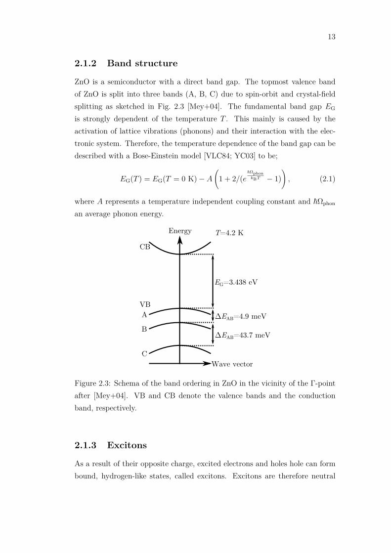
2.1.2 Band structure

ZnO is a semiconductor with a direct band gap. The topmost valence band

of ZnO is split into three bands (A, B, C) due to spin-orbit and crystal-field

splitting as sketched in Fig. 2.3 [Mey+04]. The fundamental band gap EG

is strongly dependent of the temperature T . This mainly is caused by the

activation of lattice vibrations (phonons) and their interaction with the elec-

tronic system. Therefore, the temperature dependence of the band gap can be

described with a Bose-Einstein model [VLC84; YC03] to be;

EG(T ) = EG(T = 0 K) − A

(1 + 2/(e

~Ωphon

kBT − 1)

), (2.1)

where A represents a temperature independent coupling constant and ~Ωphon

an average phonon energy.

Energy

Wave vector

CB

VB

EG=3.438 eV

EAB=4.9 meV

EAB=43.7 meV

T=4.2 K

C

B

A

Figure 2.3: Schema of the band ordering in ZnO in the vicinity of the Γ-point

after [Mey+04]. VB and CB denote the valence bands and the conduction

band, respectively.

2.1.3 Excitons

As a result of their opposite charge, excited electrons and holes hole can form

bound, hydrogen-like states, called excitons. Excitons are therefore neutral

14

and able to move freely in the crystal. The kinetic energy Eke of the exciton

is connected to the electron and hole wave vectors, ~ke and ~kh, via:

Ek( ~K) =~

2 ~K2

2M, (2.2)

where ~ is the reduced Planck’s constant, ~K = ~ke +~kh the exciton wave vector

and M the exciton mass which is given by the sum of the effective electron

and hole mass M = me + mh. Similar to the hydrogen atom the exciton has

quantized eigenenergies EN according to:

Ex,n( ~K) = EG − R∗

n2+ Ek( ~K), (2.3)

with EG being the band gap energy, n the principal quantum number (n =

1, 2, 3...) and R∗ the Rydberg energy for the exciton which is given by:

R∗ =

(µ

m0ǫ2e

)× 13.6 eV. (2.4)

Here, µ = (memh)/(me + mh) = 0.19m0 is the reduced exciton mass, m0 the

electron rest mass and ǫe the effective static dielectric constant [Kli+10a]. The

radius of the exciton rn with the quantum number n is given by:

rn = n2m0

µǫeaB, (2.5)

with aB = 0.053 nm being the hydrogen Bohr radius. According to Ref.

[Kli+10a] and references therein, the excitonic Rydberg energy for A-, B-,

and C- excitons is R∗ = (59 ± 1) meV resulting in an exciton Bohr radius of

rn=1 = 1.8 nm. As the exciton Bohr radius exceeds the lattice constants the

excitons in ZnO are called Wannier excitons.

2.1.4 Phonons

A phonon is the quantum of a lattice vibration mode. As the primitive unit

cell of wurtzite ZnO contains two zinc and two oxygen atoms twelve phonon

modes are present [Kli07]. They can be separated in three acoustical and nine

optical modes. The irreducible representation of the phonon modes is:

Γ = 2A1 + 2B1 + 2E1 + 2E2, (2.6)

15

symmetry energy (meV) degeneracy dipole allowed

E2 low Γ6 12.3 2 no

B1 low Γ3 29.7 1 no

E2 high Γ6 54.5 2 no

B1 high Γ3 66.9 2 no

A1 Γ1 TO 47.1 1 yes

LO 71.5

E1 Γ5 TO 50.8 2 yes

LO 72.5

Table 2.1: ZnO optical phonon properties at the Γ-point of the Brillouin zone,

adopted from [Kli07]

where the A- and B-modes are onefold and the E-modes twofold degenerated.

The A1 and E1 phonons are optically dipole allowed yielding longitudinal (LO)

and transversal (TO) resonance energies. The ZnO phonon energies are listed

in Table 2.1. The calculated phonon dispersion is shown in Fig. 2.4 together

with experimentally obtained data (see Ref. [Ser+04] and references therein).

In ZnO, the polariton1-phonon interaction plays an important role as it is

highly probable that an polariton decays under emission of a second polari-

ton and one or more LO phonons [Vos+06; Sha+05; Tai+10]. This leads to

a maximum in the emission intensity in luminescence experiments spectrally

positioned at LO phonon replica of the free exciton resonance energies. This

holds especially at elevated temperatures (> 80 K [Tai+10]), where defect

bound excitons (DBX) are thermally dissociated. The polariton-phonon inter-

action as a gain process is described in more detail in Sec. 2.4.1.2. Furthermore,

the (exciton-)polariton-phonon interaction leads to absorption bands in the di-

electric function (DF) which are situated in the vicinity of multiples of the LO

phonon energies above the excitonic ground-states [LY68; Sho+08; Neu15].

1The term polariton refers to exciton-polaritons as introduced in Sec. 2.2.1

16

0.0

12.4

24.8

37.2

49.6

62.0

74.4

Energ

y (

meV

)

Figure 2.4: Ab initio calculated phonon dispersion in ZnO, adapted

from [Ser+04]

2.2 Linear light-matter interaction

This section deals with phenomena which occur when a bulk material interacts

with electromagnetic waves. First, Maxwell’s theory is introduced which allows

to model the response of matter to an electromagnetic wave. Thereby, the

focus is set on dielectrics and semiconductors as these materials are used for

the microcavities being investigated within this thesis. The so called polariton

equation is introduced which follows directly from Maxwell’s equations [Max65]

and describes the allowed frequencies of the EM wave within the material

in dependence on the wave vector which is called dispersion relation. The

solutions of the polariton equation are discussed in detail for two limiting

scenarios. On the one hand, incorporating complex-valued wave vectors and

a real-valued energy gives the steady state description which differs from the

case which incorporates real-valued wave vectors and complex-valued energies.

The latter case is useful to describe temporal decay. In general, both situations

are important but a detailed description is missing in literature. The resulting

dispersion relations are deduced for bulk crystals and are important for the

analytical description of cavity polaritons which will be introduced later in this

Chapter.

17

2.2.1 Maxwell Theory

The formalism of classical electro-dynamics is fully covered by Maxwell’s set

of equations [Max65] which read in the macroscopic form [Kli12]:

∇ · ~D = ρ, (2.7)

∇ · ~B = 0, (2.8)

∇ × ~E = − ~B, (2.9)

∇ × ~H = ~D +~j. (2.10)

Equations (2.7) and (2.8) are known as Gauß’s laws which describe the elec-

tric charge density ρ as a source of the electric displacement ~D and the non-

existence of magnetic monopoles of the magnetic flux density ~B, respectively.

Faraday’s and Ampere’s laws (Eq. (2.9) and Eq. (2.10)) state that temporally

varying magnetic and electric fields (~H and ~E) generate each other. Further-

more, the presence of an electrical current density ~j creates a magnetic field.

The so called material equations for the description of the response of matter

are given by [Kli12]:

~D = ǫ0~E + ~P = ǫ0

~E + ǫ0χ~E = ǫ0ǫ~E, (2.11)

~B = µ0~H + ~M = µ0µ~H. (2.12)

Equation (2.11) states that the electric displacement is constituted by the ap-

plied electric field plus the polarization field ~P, while the magnetic flux density

is given by the magnetic field and the magnetization ~M. The unit-less quan-

tities ǫ and µ are the dielectric function (DF) and the magnetic permeability

which are in general tensors of order two. Within this thesis it will always be

referred to the case of non-magnetic (µ = 1), current-free (~j = 0) and charge-

free (ρ = 0) matter. In order to derive the wave equation for the electric field

under these conditions, the rotation operator is applied to Eq. (2.9) which

yields:

∇ × ∇ × ~E = − ∂

∂t∇ × ~B. (2.13)

Using Eq. (2.7) and substituting Eq. (2.10) in (2.13) yields:

∆~E = µ0~D, (2.14)

18

with ∆ ≡ ∇2 being the Laplace operator. Applying the material equa-

tion (2.11) and with the definition of the vacuum speed of light, c2 = 1/(µ0ǫ0),

one arrives at the wave equation for the electric field:

~E =c2

ǫ∆~E. (2.15)

The wave equation can be solved by a harmonic plane wave (PW) ansatz:

~E(~x, t) = ~E0ei(~k~x−ωt), (2.16)

with ~k being the wave vector and ω the angular frequency.

Excursus: Dielectric function in optically uniaxial crystals

In an isotropic medium the DF ǫ is a scalar quantity. But for wurtzite ZnO

which plays a major role in all samples which will be discussed in the experi-

mental sections of this thesis, this is insufficient as ZnO is an uniaxial material.

The corresponding DF is represented by a tensor of the form:

ǫ =

ǫ⊥ 0 0

0 ǫ⊥ 0

0 0 ǫ‖

, (2.17)

with ǫ⊥ and ǫ‖ being the complex-valued DF for electrical field polarization

perpendicular and parallel to the optic axis, respectively. The optic axis in

ZnO is aligned parallel to the crystal’s c-axis. A direct consequence of the

uniaxiality is the anisotropy of the index of refraction n with respect to the

optic axis if the electric field vector has a non-vanishing projection on the optic

axis. If θ denotes the angle between the wave vector ~k and the optic axis, then

the extraordinary refractive index neo can be calculated to be:

1n2

eo

=sin θ2

ǫ⊥

+cos θ2

ǫ‖

. (2.18)

For the so called ordinary ray with the polarization perpendicular to the optic

axis the index of refraction is independent of the direction of the wave vector~k:

no =√ǫ⊥. (2.19)

For ZnO, ǫ‖ and ǫ⊥ differ strongly, especially in the spectral range in the

vicinity of the band gap. This is caused by the different selection rules for

19

the coupling of dipole allowed electronic transitions to light which is polarized

perpendicular or parallel to the crystal’s c-axis. According to the selection

rules, the C-exciton strongly couples to light with ~E ‖ ~c and ~k ⊥ ~c. For this

configuration, the A-exciton is forbidden and the B-exciton is only weakly

observable. For the opposite case (~E ⊥ ~c and ~k ⊥ ~c), the C-exciton is barely

detectable, whereas A- and B-excitons are allowed [Özg+05; Kli12].

2.2.2 Polariton equation/dispersion relation

The PW ansatz given by Eq. (2.16) is only a solution of the wave equa-

tion (2.15) if the following restriction is fulfilled connecting the wave number

with the angular frequency:

~k2 = ǫ(ω

c

)2

. (2.20)

This equation is typically referred to as polariton equation or dispersion rela-

tion [Kli12] and is identical for the classical approach as well as for the quantum

mechanical one [Hop58].

Excursus: homogenous and inhomogenous plane waves

At this point, it has to be mentioned that ~k = ~k is in general a complex quan-

tity, even if the DF ǫ and the frequency ω are real-valued. In order to separate

the complexity which is connected to the DF ǫ, from the complexity which is

connected to a complex direction vector ~n, one can write [Jac82; DAP94a]:

~k =√ǫω

c~n, (2.21)

with a real-valued frequency ω and with ~n · ~n = 1. Following the definition

in Refs. [Jac82; DAP94a], if ~n is complex, the wave is called inhomogenous

plane wave (IPW). Otherwise it is an homogenous plane wave (HPW). If ~n is

complex, the planes of constant phase and constant amplitude are no longer

parallel. For IPWs in general, Snell’s law and the Fresnel formulae have to be

modified [DAP94a]. A famous example for an IPW in a transparent medium

(real-valued DF) is the evanescent wave at an interface in the case of total

internal reflection (TIR). Another example for IPWs is given if a HPW is inci-

dent under an oblique angle out of a non-absorbing material on the interface

to an absorbing medium. In this case, the transmitted wave is an IPW as the

planes of constant amplitude are always parallel to the interface as a result of

20

the conservation of the real in-plane wave vector component. This is the usual

case in reflectivity measurements. In contrast to that, in photoluminescence

(PL) measurements light is typically generated closely to the interface within

the absorbing medium. The resulting wave within the absorbing medium is a

HPW as there is no restriction for a real-valued in-plane wave vector compo-

nent and thus, the planes of constant phase and amplitude are parallel. More

details about Snell’s law, the Fresnel formulae and the Poynting vector for

HPWs and IPWs can be found in Appendix A.4.1.

Bulk polariton: complex-valued wave vector and/or frequency

Regarding HPWs, the vector character of ~k in Eq. (2.20) can be dropped ac-

cording to k2 ≡ ~k2 [Kli12]. The polariton equation (2.20) is then given by:

k =√ǫω

c. (2.22)

For a HPW and a complex DF, i.e. if absorption is present, the question

arises if the quantities k and ω in the polariton equation (2.22) are real or

complex. The answer to this question depends on the actual situation in

the experiment as also stated by Klingshirn [Kli12]. Many authors prefer a

complex wave number k and a real-valued frequency ω [DAP94a; Kli12] when

the polariton equation (2.22) is introduced and losses are included. A real

frequency implies a monochromatic wave with an infinite temporal expansion,

as time and frequency are connected by a Fourier transformation (FT) [Kli12].

Under this (experimentally not exactly realizable) condition, the polariton

equation (2.22) can be written as:

k = Re[k] + Im[k] =√ǫ(ω)

ω

c≡ n(ω)

ω

c, (2.23)

with n(ω) = n(ω) + iκ(ω) being the complex index of refraction. If this ansatz

is inserted in the PW Eq. (2.16), positive values of κ lead to a spatially damped

wave which can be written for a HPW propagating in x-direction as:

~E(~x, t) = ~E0ei(n ω

cx−ωt)e−κ ω

cx. (2.24)

Real and imaginary parts of the wave number k are simply given by:

Re[k] = nω

c, (2.25)

Im[k] = κω

c. (2.26)

21

From Eq. (2.24) one can deduce the factor describing a constant phase in time

and space:

nω

cx− ωt = const. (2.27)

Multiplication with the operator ∂/∂t yields the well known phase veloc-

ity [Som50; LL80; Kli12]:

vph =∂x

∂t=

ω

nωc

=ω

Re[k]=c

n. (2.28)

In contrast to that, a complex frequency ω = ω0 − iωi with ωi > 0 and real-

valued wave number k imply a temporally decaying wave which is extended

over an infinite distance with a spatially independent amplitude. For this (also

not perfectly realizable) case, the polariton equation (2.22) is written as:

k = n(ω)ω

c. (2.29)

Combining equations (2.29) and (2.16), yields for a HPW propagating in x-

direction:~E(~x, t) = ~E0e

i((n+ κ2

n)

ω0c

x−ω0t)e−ωit. (2.30)

Here, it was used that k has to be real in (2.29) which fixes the imaginary part

of the frequency:

ωi =κ

nω0, (2.31)

which is a different result compared to the case for a complex wave number (see

Eq. (2.26) multiplied with c) as the factor n−1 is added. The most interesting

detail resulting from the assumption of a temporally decaying wave (complex

frequency ω) in combination with a real-valued wave number k is the fact that

the wavelength in absorbing matter is altered compared to the case with a real

frequency according to:λ0

n→ λ0

n+ κ2

n

, (2.32)

with λ0 = 2πc/ω0 being the wavelength in vacuum. For the phase velocity

in presence of temporal decay (and real k), a different result is found from

Eq. (2.30) as a result of the modified wavelength within the material:

(n+κ2

n)ω

cvph − ω0t = 0, (2.33)

which results in:

vph =c

n+ κ2

n

. (2.34)

22

A problem arises, if it is necessary to incorporate temporal losses in order to

calculate the polariton modes in presence of absorption (see Eq. (2.29). For this

case the complex DF has to be known as a function of the complex frequency

ω. Therefore, if only a tabulated complex DF ǫ(ω) of the material of interest

is known, it has to be modeled with a functional expression for practical use.

2.2.3 The bulk polariton in the presence of a dipole al-

lowed transition

From here on, the (complex) frequency will be replaced by the (complex)

energy according to E = ~ω = E0 − iγ. If a HPW travels through vacuum

or a homogeneous medium with a supposedly constant refractive index n and

without absorption (κ = 0), the polariton equation (2.20) gives a linear relation

between E and k:

E(k) = ~ck

n. (2.35)

In the presence of a dipole allowed transition the DF ǫ and therefore the

complex index of refraction n =√ǫ become strongly energy-dependent. The

DF describing a single dipole allowed transition depends on the photon energy

E, the resonance energy E0, the damping γ, and the coupling strength f

between the electromagnetic field and the oscillator. If a possible wave vector

dependency of E0, f , and γ is ignored (i.e. no so called spatial dispersion), the

DF ǫ can be described by a Lorentzian [Kli12] in the form:

ǫ(E) = ǫ1 + iǫ2 = 1 +f

E20 − E2 + iE2γ

. (2.36)

The real and imaginary parts of the DF for a single Lorentzian oscillator are

plotted exemplarily in Fig. 2.5 for the cases without (γ = 0) and with (γ > 0)

losses. The damping γ describes in good approximation the half width at

half maximum (HWHM) of ǫ2. In the case of vanishing damping (γ → 0),

ǫ2 is represented by a δ-function at the resonance energy E0 [Kli12]. For

energies far below the resonance, Eq. (2.36) yields ǫ1(E → 0) = 1 + f/E20 ,

whereas for high energies ǫ1(E → ∞) = 1 holds. Therefore, the presence of

low energy resonances has a vanishing influence on the DF in the vicinity of a

well separated resonance higher in energy. In contrast to that, the presence of

higher energy resonances has to be included as a constant background constant

23

ǫb. As a real material always shows several resonances, the resulting DF in the

vicinity of a single isolated resonance energy E ′0 can be written as:

ǫ(E) = ǫb +f ′

E′20 − E2 + iE2γ′

. (2.37)

Figure 2.5: Simulated dielectric function of a Lorentzian oscillator for two

different values of the damping γ for a constant oscillator strength f . In the

case of vanishing damping (γ → 0), the imaginary part of the DF is represented

by a δ-function and the real part possesses a pole at E = E0.

In order to obtain the allowed energies in dependence on the wave number

in the vicinity of a single resonance, Eq. (2.37) has to be combined with the

polariton equation (2.22). If absorption is fictively present as a δ-function,

both, energy and wave vector are real-valued quantities in bulk materials. The

dispersion relation E(k) is then given implicitly by:

~2c2k2

E2= ǫb +

f

E20 − E2

. (2.38)

For this case (γ = 0), Eq. (2.38) has two real and positive solutions in E for

each k,

E+,− =1√2ǫb

√f + ~2c2k2 + ǫbE2

0 ±√

−4~2c2k2ǫbE20 + (f + ~2c2k2 + ǫbE2

0)2,

(2.39)

24

Figure 2.6: a) Calculated polariton dispersion relation in the vicinity of a res-

onance (solid lines) without damping (γ = 0). The dashed lines represent the

photon dispersions in vacuum and in a medium with refractive index√ǫb. The

spectral range between E0 and EL (dotted lines) indicates the restrahlenbande.

b) Calculated squared Hopfield coefficients |X|2 (black) and |C|2 (gray) for the

LPB from a). The Hopfield coefficients for the UPB are given under exchange

of |X|2 and |C|2, respectively.

25

which are plotted in Fig. 2.6 together with the dispersion relation in vacuum

and in a medium with a background dielectric constant of ǫb. These two solu-

tions are generally known as upper and lower polariton branch (UPB and LPB)

of the so called bulk polariton. The LPB dispersion flattens by approaching

the resonance energy E0. It is then called "exciton-like", if the resonance en-

ergy E0 is an excitonic transition. For k = 0 the UPB coincides with the so

called longitudinal (exciton) energy EL which is given by:

E2L − E2

0 =f

ǫb

. (2.40)

The difference EL − E0 is called longitudinal-transversal (L-T) splitting. The

minimum energy of the UPB, EL, coincides for k = 0 with the longitudinal

polariton branch. The longitudinal branch exists only within the material and

thus, is not able to couple into vacuum2. Therefore, it is not obeyed in the

discussion of the polariton as presented in this thesis. Taking into account a

non-vanishing broadening (γ > 0), yields a reduced L-T splitting:

E2L − E2

0 =f

ǫb

− γ2. (2.41)

For large values of γ this has an influence on the well known Lyddane-Sachs-

Teller which changes:ǫ(E = 0)ǫ(E → ∞)

=E2

L

E20

+γ2

E20

. (2.42)

As spatial dispersion (k-dependence of E0 and f) which is present at excitonic

resonances, is neglected, this simplification predicts vanishing optical density

between E0 and EL which is in general not correct [MM73]3. If Eq. (2.38) is

evaluated at the crossing point of the uncoupled resonances at k = E0/(~c)√ǫb,

it reduces to:E2

E20

=ǫb

ǫ. (2.43)

The solution of this equation gives the normal mode- or Rabi-splitting Ω be-

tween UPB and LPB, and is found in the case of vanishing damping to be:

Ω =

√f

ǫb

(2.44)

2Out-coupling is possible by coupling to the evanescent wave of a prism put onto the

sample’s surface.3Ignoring spatial dispersion in modeling e.g. reflectivity spectra of a bulk crystal results

in an artificially increased broadening of the resonance within the model.

26

The deduction of Eq. (2.44) can be found in Appendix A.1.

If a finite broadening of the resonance γ is taken into account, the situation

regarding the polariton dispersion is more complicated as the question arises

which model is more appropriate: the model excluding temporal losses (real-

valued energy), as given by Eq. (2.23), or the model which includes temporal

decay (complex-valued energy) in the limit of a real-valued wave vector as

given by Eq. (2.29). In Fig. 2.7 the (complex) polariton branches for the two

different models are plotted. For energies well separated from the resonance

energy, both models give similar results for the LPB and UPB. In contrast to

that, in the vicinity of the resonance energy (E0 − γ ≤ E ≤ E0 + γ), both

models give very different results. Regarding the case of a complex wave vector

and a real-valued energy, the polariton equation (2.23) yields one real branch

which exhibits an anomalous dispersion (∂E/∂Re[k] < 0) in the vicinity of

the resonance. Its imaginary part is similarly shaped as the imaginary part

of the complex index of refraction. Both facts are not surprising as the real

(imaginary) part of the wave vector is given by the real (imaginary) part of

the complex DF multiplied with E/(~c):

Re[k(E)] = n(E)E

~c= n(E)k0 (2.45)

and

Im[k(E)] = κ(E)E

~c= κ(E)k0. (2.46)

In experiments, the polariton branch with anomalous dispersion will hardly

be observable due to the strong absorption being present in the corresponding

spectral range. If the model with a complex-valued energy and a real-valued

wave number is evaluated in the vicinity of a resonance, two distinct polariton

branches (LPB and UPB) are recovered (see Fig. 2.7). Their splitting at the

crossing point of the uncoupled modes is reduced by the broadening γ according

to (see Appendix A.1):

Ω =

√f

ǫb

− γ2. (2.47)

This relation predicts a vanishing splitting for γ2 > f/ǫb which marks the

transition from the so called strong to the weak coupling regime. In the strong

coupling regime, the appearance of the mode splitting between the lower and

upper polariton branch (LPB and UPB) allows for the observation of Rabi

27

oscillations as a result of the coherent superposition of LPB and UPB. This

oscillations in intensity with the frequency Ω/~ can classically be understood

as the beating appearing if two waves with different frequencies are coherently

superimposed [Kli12].

Figure 2.7: Calculated bulk polariton branches for two different models re-

garding spatial or temporal decay in the vicinity of a resonance E0 with finite

broadening γ > 0. In b) the corresponding real parts are plotted whereas in

a) and c) the imaginary parts of the polariton branches are plotted.

The splitting in UPB and LPB and their dispersions for the case of a com-

plex energy (frequency) can also be derived in good approximation by the

quantum mechanical coupled oscillator model, with a Hamiltonian that can

be written as:

H =

EC V

V EX

, (2.48)

with EC(k) = ~ck/√ǫb being the polariton dispersion for a vanishing oscillator

strength, EX = E0 − iγ0 being the complex excitonic transition energy, and

28

V = 0.5√f/ǫb being the exciton-photon coupling constant. In the following,

the polariton dispersion for f = 0 will be denoted as bare cavity mode disper-

sion EC(k). The eigenvalues of the Hamiltonian (2.48) are the UPB and LPB.

Excitonic broadening due to damping is introduced as imaginary part of EX.

The splitting Ω between LPB and UPB at the crossing point of the uncoupled

modes is identically to that derived before from Maxwell’s equations in the

limit of complex energies and a real-valued wave number k:

Ω =√

4V 2 − γ2 =

√f

ǫb

− γ2. (2.49)

The polariton branches obtained from Hamiltonian (2.48) are plotted in Fig. 2.8

together with the branches derived by Maxwell’s equations in the limit of a

complex energy and a real-valued wave number. Small deviations in the com-

plex energies are found.

The Hamiltonian (2.48) describes the mixing of the uncoupled eigenstates

of the photon and the resonance (exciton/phonon etc.). The properties of the

mixed states can be quantified with the squares of the Hopfield coefficients |X|2

and |C|2 ( |X|2 + |C|2 = 1), describing their excitonic and photonic fraction,

respectively. The Hopfield coefficients for the LPB are given by:

|X|2 =12

1 +

δ(k)√δ(k)2 + 4V 2

(2.50)

and

|C|2 =12

1 − δ(k)

√δ(k)2 + 4V 2

. (2.51)

The corresponding formulae for the UPB are given under exchange of |X|2 and

|C|2. The quantity δ(k) = EC(k) −EX(k) describes the detuning between the

uncoupled modes. For δ(k) = 0 the corresponding coupled modes have equal

contributions of both involved resonances, yielding |X|2 = |C|2 = 0.5. The

wave number dependence of the Hopfield coefficients for a LPB close to the

crossing point of the uncoupled modes is drawn in Fig. 2.6 b).

2.3 Cavity polaritons

This section deals with polaritons in structures of reduced dimensionality of

the photonic system (cavities). General differences and similarities to the bulk

29

Figure 2.8: Comparison of the polariton branches derived from Maxwell’s equa-

tions (black lines) and from the quantum mechanical coupling Hamiltonian

(gray lines). Imaginary and real parts are plotted in a) and b), respectively.

30

polariton, as presented before, are described. Some general features are pre-

sented regarding the eigen-energies and broadenings of resonant cavity modes.

Furthermore, the mode splitting in the vicinity of dipole allowed transitions

is discussed and the regimes of weak and strong coupling for cavity polaritons

are introduced. As examples for cavities which are investigated within this

thesis, the polariton modes of Fabry-Pérot (FPM) and hexagonal whispering

gallery mode (WGM) cavities are introduced. Regarding nomenclature, the

term active cavity will be used, if at least one dipole allowed resonance accord-

ing to Eq. (2.37) is present in the spectral (energetic) range of interest in the

cavity structure.

2.3.1 Basic properties

2.3.1.1 Ground-states of cavity modes confined in one dimension

If a photonic or polaritonic wave is confined in a cavity with round trip length

Leff , the (vacuum) wave number will be quantized according to:

k⊥ = N2πLeff

. (2.52)

The term Leff refers to the fact that due to additional phase shifts at bound-

aries the cavity length L is effectively shortened or increased in terms of the

phase evolution in space. In the following, general expressions are derived for

the eigen-energies and broadenings taking into account these additional phase

shifts. Therefore, a cavity of total length L is considered including m identical

mirrors with the, in general complex, reflectivities r = |r|eiφ. The cavity is

assumed to enclose a material with the complex index of refraction n. In order

to obtain the allowed complex wave numbers kN (or complex eigen-energies

EN), phase matching after one round trip has to be fulfilled. Mathematically,

this can be expressed by:

rmeinEN~c

L = C, (2.53)

with C being real ensuring phase matching and C ∈ [0, 1] accounting for

material and mirror losses after one round trip. In order to account for angular

dispersion, L is replaced by L cos θ with θ being the angle measured between

the confinement direction and the wave vector. Typically, the mirror losses

31

|r|m in Eq. (2.53) are incorporated in an effective extinction coefficient κ′ by

the definition [Yar88; Kap98]:

|r|me−κEN~c

L ≡ e−κ′ EN~c

L, (2.54)

which yields for the effective extinction coefficient κ′:

κ′ = − ~c

ENLln |r|m + κ. (2.55)

The cavity polariton equation (2.53) can now be written as:

eimφei(n+iκ′)EN~c

L = C. (2.56)

At this point, the same problem arises regarding real and/or complex wave

numbers and energies as in the case of the bulk polariton (see discussion in

Sec. 2.2.2). In the experimental limit which is described by a complex wave

number and a real energy (frequency), one round trip leads to a reduced am-

plitude which is expressed by the effective extinction coefficient κ′ via:

C = e−κ′ EN~c

L. (2.57)

The mode equation is then written as:

eimφeinEN~c

L = 1. (2.58)

The real part of the wave number in vacuum is then simply given by:

kN,0 =EN

~c=

1nL

(N2π −mφ), (2.59)

with N being an integer. The imaginary part of the wave number is given by:

kN,i = κ′kN,0 = − 1L

ln |r|m + κEN

~c. (2.60)

On the other hand, for the incorporation of temporal decay (described by

a complex energy EN → EN = EN − iγN in Eq. (2.56) in the limit of a

real-valued wave number, one spatial round trip does not lead to a reduced

amplitude which is expressed by:

C = 1. (2.61)

Equation (2.56) is then written as:

eimφei(n+iκ′)EN~c

L = 1. (2.62)

32

The mirror losses again are considered in the effective extinction coefficient

κ′. The ansatz of a real-valued wave number, complex energies, and the phase

matching condition yields for the real part of the complex mode energies EN :

EN =~c

nL(N2π −mφ) − κ′

nγN =

~c

(n+ κ′2

n)L

(N2π −mφ), (2.63)

and for the broadenings γN :

γN =κ′

nEN =

κ

nEN − ~c

nLln |r|m ≡ γabs + γC. (2.64)

In accordance with the results obtained before for bulk polaritons the presence

of temporal decay given by mirror (γC) and absorption losses (γabs) alters the

wavelength in matter. This directly influences the resonance energies EN due

to the phase matching condition. Equations (2.63) and (2.64) are implicit

formulations for the complex mode energies. As the explicit expressions are

lengthy, they can be found in the Appendix A.2. An important quantity of the

cavity structure is its quality factor Q being defined as the ratio of the average

stored energy in the cavity and the energy loss per round-trip cycle which can

be measured as:

Q =EN

γN

. (2.65)

As discussed before, the inclusion of temporal decay (complex energies)

changes the eigen-energies compared to the case where only spatial decay (com-

plex wave numbers) is considered. This results from the fact that temporal

decay changes the wavelength in matter according to λ0/n → λ0/(n + κ′2

n).

Assuming that this model-dependent difference becomes recognizable if κ′2

n>

0.01n, implies that κ′ > 0.1n. This is connected with a broadening of the

corresponding mode of γN > 0.1EN according to Eq. (2.64). For the cavi-

ties discussed within this thesis EN ≈ 3 eV holds which requires broadenings

(HWHM) in the order of γN ≈ 300 meV to be present in order to measure a

significant change of the eigen-energies depending on the experimental situa-

tion (or applied model). As the observed modes within this thesis are typically

at least one order of magnitude smaller, the term κ′2

nin Eq. (2.63) becomes

negligibly small and both models (Eq. (2.59) and (2.63)) predict the same

ground-state eigen-energies. The cavity polariton ground-state eigen-energies

are therefore given in the low loss limit (κ′ << n) by:

EN =~c

nk⊥ =

~c

nLeff

N2π, (2.66)

33

with k⊥ = N2π/Leff and:

L−1eff = L−1(1 −mφ/(N2π)). (2.67)

Obviously, for large mode numbers N and only a few reflections m within

one cavity round trip, the influence of the phase shift upon reflection becomes

small and the effective cavity length approaches the real one (Leff ≈ L).

Excursus: Cavity polariton modes as poles of the complex reflec-

tion coefficicent

In literature dealing with cavity polaritons and temporal decay (complex en-

ergies), typically a condition for resonant modes different from Eq. (2.62)

is given [And94; Sav+95; KK95; VKK96]. For a planar Fabry-Pérot cavity

(m = 2, L = 2d):

r2eikL = r2ei(nEN~c

2d) = 1 (2.68)

is considered, equivalently to the formulation T22 = 0 or rtot = −T21/T22 → ∞,

with rtot being the complex reflection coefficient and with Ti,j being the transfer

matrix of the entire cavity structure after [Bra76; And94]. This is exactly the

same as the threshold condition for lasing as given in Refs. [Mak91; Mak93;

Mak94; Kim+99]. One can easily see that Eq. (2.68) calls for complex wave

numbers k expressing gain in order to compensate for the mirror losses, if

|r|2 < 1 holds. The solutions of mode condition (2.68) in terms of complex

energies are given by:

EN =~c

2nd(N2π − 2φ) − κ

nγN , (2.69)

and

γN =κ

nEN − ~c

2ndln |r|2 = γabs + γC. (2.70)

The resulting broadenings γN are identical to the result obtained before (see

Eq. (2.64)) in the limit of complex energies and a real wave number. In contrast

to that, the real part of the mode energiesEN differ. Again, explicit expressions

for Eqs. (2.69) and (2.70) can be found in the Appendix A.2. The results

obtained here from the complex poles of the reflection coefficient, predict a

vanishing influence of the mirror losses on the mode energies if the cavity is

transparent (κ = 0 in Eq. (2.69)). But this can only be true, if no temporal

losses are incorporated, as shown by the derivation of Eq. (2.59) in the limit of

34

real energies and complex wave numbers. This vanishing effect of the mirror

losses on the real part of the mode energies is a direct consequence of the gain

which is intrinsically introduced by the mode condition (2.68) and exactly

compensates the mirror losses. This result has no physical meaning if complex

mode energies have to be calculated for cavities without a gain source in the

presence of mirror losses. Nevertheless, for cavities in the limit of vanishing

mirror losses (|r|2 → 1), the complex energies obtained by Eq. (2.68) yield the

same results as calculated in this section from the definition of a mode as a

consequence of phase matching after one cavity round trip in the limit of real

wave numbers. In Figure 2.9, the real part of the mode energies for the two

models are compared with the model including only real energies. Thereby,

the extinction coefficient and mirror reflectivity is varied.

2.3.1.2 Cavity polariton dispersion

In section 2.3.1.1, the ground-state energies of one dimensionally confined cav-

ity modes were discussed following from the quantization of the wave number

k → k⊥. If propagating states are included, this can be expressed by the

in-plane wave number k‖ which is vectorially added to the ground-state wave

number:

k →√k2

⊥ + k2‖. (2.71)

The cavity polariton mode equation in the limit of real-valued energies and

complex wave numbers is given by:

EN(k‖) =~c

n

√k2

⊥ + k2‖. (2.72)

Considering complex energies (and real wave numbers) under the assumption

of low mirror losses (|r|m ≈ 1), the polariton dispersion is given by:

EN(k‖) = Re[n−1]~c√k2

⊥ + k2‖ =

~c

n+ κ2

n

√k2

⊥ + k2‖, (2.73)

Both formulae are in most cases implicit representations for EN as the refrac-

tive index typically strongly depends on energy. If the k‖ dependency of the

phase shifts φ during reflection is negligible, cavity modes show a minimum en-

ergy at k‖ = 04. For a cavity containing vacuum (n = 1), equations (2.72) and

4Due to the incorporation of resonant grating filters as mirrors, whose complex reflectivity

is strongly dependent of k‖, it is possible to design dispersionless cavity modes or modes

with an energetic maximum at k‖ = 0, as shown in Ref. [BKC16].

35

0.00 0.05 0.100.990

0.992

0.994

0.996

0.998

1.000

0.7 0.8 0.9 1.0

b)

Rel

ativ

e m

ode

ener

gy s

hift

Extinction

T22=0

Model:E, k~

0.90

0.95

Reflectivity:0.99

a)

T22=0

Model:

0.1

0.01

Reflectivity |r|2

Extinction:0.001

E, k~

Figure 2.9: Relative shift of the cavity mode energy’s real part for different

mode conditions as indicated by black and gray lines for a variation of the

extinction coefficient κ (a) or of the reflectivity |r|2 (b). Different line plot

styles (solid, dashed, dotted) indicate example values of the quantity which is

not continuously varied in the respective plot. The relative energy refers to

the mode energy with κ = 0 and |r| = 1 as also given by the mode condition

excluding temporal decay were losses do not influence the real part of the

resonance energies. The graphs are calculated for a fictive cavity with thickness

2d = L = 1 µm, refractive index n = 2, mode order N = 1, and for a vanishing

phase shift upon reflection φ = 0.

36

(2.73) are identical with the energy-momentum relation for a massive particle

with rest energy E0 = ~ck⊥ and momentum p = ~k‖ as known from special

relativity [Ein05; LL67]:

E(p) =√E2

0 + (pc)2. (2.74)

Therefore, the spatial confinement of a polaritonic or photonic (in the case of

vacuum) mode can be understood as an introduction of an effective rest mass

meff,0 for the cavity mode. The effective mass meff is defined by the temporal

change of the group velocity ~vg as a result of a force ~F introduced by a potential

gradient ∇Φ = −~F :

~vg = m−1eff~F . (2.75)

Introducing the relations ~vg = ∇~k‖ω(~k‖) and ~F = ~~k‖ yields for the effective

mass meff :

m−1eff = ~

−2∆~k‖E(~k‖). (2.76)

Evaluating Eq. (2.76) in combination with Eq. (2.72) at k‖ = 0, results in the

effective rest mass meff,0 given by:

meff,0 = EN(k‖ = 0)(n

c

)2

. (2.77)

In the case of a cavity containing vacuum (n = 1), Einstein’s famous rela-

tion between (rest-)mass and Energy is recovered: E = meff,0c2. For cavities

containing a polarizable medium (n 6= 1), the speed of light has to be re-

placed by the phase velocity. In Fig. 2.10 the lowest energy modes according

to Eq. (2.72) are plotted. The mode with N = 0 belongs to the guided modes

which behave as free photons if the cavity contains vacuum, or as a bulk po-

lariton in the presence of dipole allowed transitions. Modes with N > 0 show

the typical hyperbolic behavior with an energetic minimum at k‖ = 0. Equa-

tion (2.77) predicts an increasing rest mass with increasing ground state energy

EN(k‖ = 0) which is clearly visible by the reduced curvature with increasing

N at the corresponding ground-state energy. Regarding one single mode, with

increasing value of k‖, the effective mass increases according to:

meff(k‖) =~n

c

(k2⊥ + k2

‖)3/2

k2⊥

. (2.78)

As consequence of the hyperbolic-form of Eq. (2.72), the cavity photon dis-

37

Figure 2.10: Cavity polariton mode dispersion for a constant index of refraction

n for the four lowest mode numbers N .

persion asymptotically approaches the free photon-dispersion which results in

an unbound effective mass for an increasing in-plane wave number k‖. The

effective mass description is not useful for a free photon as it cannot be further

accelerated. Therefore, the mass of the free photon is only connected to its mo-

mentum via p = mv = ~k. This, again, leads with v = c/n and k = nE/(~c)

to m = n2E/c2.

2.3.1.3 The cavity polariton in the presence of

a dipole allowed transition

If a cavity polariton mode is situated spectrally in the vicinity of a dipole

allowed transition, the refractive index n =√ǫ in equations (2.72) and (2.73)

becomes strongly energy-dependent. The solutions of Eq. (2.73) in the limit

of high quality mirrors (|r|m ≈ 1) including a single resonance as a Lorentz

oscillator are identical to the case of the bulk polariton (see Sec. 2.2.3) with

the modified wave number k →√k2

⊥ + k2‖. The solutions E1 of Eq. (2.63)

are plotted in Fig. 2.11 in the limit of a real-valued wave number, complex

energies, and under the assumption of negligible mirror losses (|r|m ≈ 1). The

bare cavity mode with N = 1 has been tuned to resonance with the dipole

38

allowed transition energy E0. If Eq. (2.72) is evaluated at the crossing point

of the uncoupled resonances at k2‖ = E2

0ǫb/(~c)2 − k2⊥, it reduces to:

E2

E20

=ǫb

ǫ, (2.79)

which is the same as Eq. (2.43) and determines the bulk polariton splitting if

spatial dispersion is neglected. Therefore, the cavity polariton splitting Ωcav

is the same as in the case of the bulk polariton if mirror losses are negligible

and the entire cavity contains the active material. The cavity mode splitting

is therefore written as:

Ωcav =

√f

ǫb

− γ2. (2.80)

Details on the derivation of the mode splitting can be found in Appendix A.1

and A.1.2.

Figure 2.11: Calculated real part of the cavity polariton dispersion relation

(solid lines) in the vicinity of a resonance E0 in the limit of real wave num-

bers and complex energies. The dashed line represents the bare cavity mode

dispersion in a medium with refractive index√ǫb.

Similar to the bulk-polariton case, also the cavity polariton dispersion in the

vicinity of a dipole allowed resonance can be approximated with a Hamiltonian

39

describing two coupled oscillators which is typically written as [Sav+95]:

H =

EC V

V EX

, (2.81)

The eigenvalues of the Hamiltonian (2.81) are given by:

E+,− = E0 +δ

2− i

2(γ0 +γC)±

√δ2

4+ V 2 −

(γC − γ0

2

)2

+i2δ(γC − γ0), (2.82)

with δ = EC − E0 being the detuning between the bare cavity mode and

the (excitonic) resonance. In general, a complex cavity mode energy EC −iγC is introduced for considering photonic losses from the cavity [Sav+95].

For resonance condition of the uncoupled modes, δ = 0, the resulting mode

splitting is given by:

Ω =√

4V 2 − (γC − γ0)2. (2.83)

This often quoted formula gives in general non-physically results in terms of a

measurable splitting as for similar valued imaginary parts γC ≈ γ0 a maximum

splitting, i.e. the bulk splitting without losses, is predicted. As it was shown

in the derivation of the complex cavity polariton eigen-energies in Sec. 2.3.1.1,

if temporal losses (i.e. absorption and mirror losses) are included as imagi-

nary parts of the complex eigen-energies, they add rather than compensate

each other. In the original paper of Savona [Sav+95], exactly this is derived

for the mode splitting measured in absorption. Hamiltonian (2.81) and the

resulting splitting, given by Eq. (2.83), yield only reasonable results, if mirror

losses are negligible (|r|m ≈ 1) or EC ≈ EC. Furthermore, if the solutions

of Hamiltonian (2.81) for a planar cavity are compared with those obtained

from commercial thin film optics software5, very different results may be ob-

tained for low mirror reflectivities, as shown in Appendix A.1.3. This results

mostly from the fact that commercial software uses standard text book for-

mulas [J A08] excluding complex energies (temporal decay) and the obtained

mode energies are by definition independent of mirror-losses as also predicted

by Eq. (2.59) for real mode energies and complex wave numbers.

5Example given: CompleteEASE by J. A. Woollam Co., Inc. [J A08]

40

2.3.1.4 Weak and strong coupling regime

The eigenvalues (2.82) of the coupling Hamiltonian (2.81) give physically rea-

sonable results for the imaginary and real parts of measurable coupled cavity

mode energies if mirror losses are small compared to the coupling constant V

or to the resonance (exciton) broadening γ. This is the case for high quality

cavities. Then, in the framework of cavity polaritons, two regimes of light-

matter interaction are distinguished. The case, where the splitting between

UPB and LPB is real, is given by:

2V > |γ0 − γC|. (2.84)

If this condition is fulfilled, the polariton system is termed to be in the strong

coupling regime (SCR) with an observable anticrossing enabling the observa-

tion of Rabi oscillations if both polariton branches are occupied. The case

of:

2V ≤ |γ0 − γC|, (2.85)

is called weak coupling regime (WCR), where no mode splitting is observable

and Rabi oscillations are suppressed due to dephasing. In this regime, the in-

fluence of the photon on the excitonic system can be treated with perturbation

theory [Sav+95] and is known as Purcell effect [Pur46]. This effect describes

the spontaneous (excitonic) emission rate in dependence on the photonic mode

density of states at the resonance. According to Fermi’s Golden rule both are

proportional to each other [Gru06], so that in the case of resonance (δ = 0) the

spontaneous emission rate is enhanced compared to the bulk case with contin-

uum photon density of states [Bay03]. Otherwise, if the photonic mode is off

resonance (δ 6= 0) destructive interference effects can lower the photonic mode

density of states below the vacuum level leading to a suppressed spontaneous

emission rate [Jak+14]. The factor which describes the change in the emission

rate in the cavity compared to the bulk (or vacuum) case, is called Purcell

factor P and is given by:

P ∝ Q (2.86)

with Q being the quality factor of the cavity mode.

Excursus: weak and strong coupling in ZnO-based cavities

In ZnO-based microcavities with a bulk-like cavity, the UPB is spectrally sit-

uated in the range close to the band gap, where absorption caused by higher

41

excitonic states and the band edge tail leads to a strong broadening of the

UPB which makes it hard to observe. This hinders the direct measurement

of the Rabi splitting. In order to decide from experimental measurements

whether the cavity is in SCR or not one has to model the bare (f = 0) cav-

ity mode dispersion to determine the detuning δ(k‖ = 0) and the bare cavity

mode broadening γC. The bare cavity mode dispersion can be modeled by ar-

tificially removing the excitonic contributions from the DF [Stu+11b; Stu11]

(s. Fig. 2.12). By modeling the experimental obtained LPB under variation

of the coupling strength gives then the splitting after Eq. (2.83), if the cavity

losses are negligible.

3.00 3.25 3.50 3.75 4.000.0

0.5

1.0

1.5

2.0

2.5

3.0

Energy (eV)

Figure 2.12: Complex index of refraction of ZnO with (solid) and without

(dashed) excitonic contributions: refractive index n (black) and extinction

coefficient κ (gray) in the vicinity of the band gap at T = 290 K for polarization

perpendicular to the optic axis of ZnO. Taken from [Stu+09].

2.3.1.5 Multi-mode cavity polariton systems

In literature dealing with polaritonic effects in the presence of several cavity

modes in the spectral vicinity of a dipole allowed transition, two very different

models are found for the description of the emerging modes. On the one

hand, an independent splitting of each bare cavity mode is predicted at the

42

electronic resonance [Tri+11; Blo+97]. On the other hand, some authors use a

model which incorporates anticrossing of the coupled modes and a crossing of

the coupled modes with the electronic resonances [Fau+09; Oro+11; Sch+10;

Die+16]. A detailed description why the latter model gives unphysical results

can be found in Ref. [Ric+15]. In this section, only a short introduction in

this topic will be given.

If the cavity round trip length L is larger than ~c/(E0√ǫb), then at least

one second bare cavity mode is able to cross the resonance E0. Figure 2.13

shows the solution of the cavity polariton equation (2.72) for the case that the

bare cavity mode with mode number N = 2 is resonant with E0. The bare

cavity mode with N = 1 is therefore situated at lower energies resulting in a

crossing point with the resonance E0 at higher k|| values. Both cavity modes

split independently of each other in an upper and lower polariton branch with

the same mode spacing Ω =√f/ǫb (for γ = 0) as derived before [Ric+15].

But this is not a general result since both, f and ǫb can be a function of the

in-plane wave vector. A further result of the independent splitting of each

bare cavity mode is the fact that single lower polariton branches can converge

at high in-plane momenta, i.e. they do not show an anti-crossing behavior

among each other. The same holds for upper polariton branches for vanishing

in-plane momenta. The independent splitting is thereby a result of the cav-

ity polariton equation (2.72) which actually represents a set of independent

equations, one for each mode number N . Therefore, the description of the

mode dispersion in terms of solutions of coupling Hamiltonians is given by

independent Hamiltonians HN of the form [Tri+11; Ric+15]:

HN =

EC,N V

V EX

. (2.87)

Furthermore, the incorporation of a second, spectrally separated and dipole

allowed transition can be incorporated by [Ric+15]:

HN =

EC,N V V

V EX,1 0

V 0 EX,2

. (2.88)

43

In-plane wave vector k|| (arb. units)

Ener

gy (

arb. unit

s)

UPB2

LPB2

UPB1

LPB1

E0

Figure 2.13: Calculated cavity polariton dispersion relation (solid lines) in the

vicinity of a resonance E0 without damping (γ = 0) for two consecutive bare

cavity modes (N = 1, 2, dashed lines). Each bare cavity mode splits into two

(UPBN ,LPBN) polariton branches with a spacing of Ω at the crossing point of

the bare cavity mode and the resonance.

2.3.1.6 Active cavities incorporating passive regions

The considerations regarding mode energies and splittings as presented in the

previous sections are true as long as the entire cavity contains the active ma-

terial with the DF ǫ(E) which is reflected in the bulk-like splitting behavior of

the cavity modes. Therefore, the knowledge of the background DF ǫb and of

the oscillator strength f fully enables the determination of the mode splitting

in bulk like cavities. Bulk-like cavities are for instance nanowires, where light

is confined between two end facets separated in the micron range or whispering

gallery mode resonators where, light is confined by total internal reflections at

the side facets [Vug+06]. Furthermore, a plan-parallel semiconductor slab also

forms a bulk like Fabry-Pérot cavity.

In contrast to bulk-like cavities, it is also possible to fabricate cavities, where

the cavity mode inside the cavity has an relative overlap x with the active

material which is remarkably smaller than unity. This is for example given in

Fabry-Pérot cavities with distributed Bragg reflectors, where the active cavity

layer typically has only a thickness of one micron or less. There, a considerable

44

part of the integrated field intensity is situated in the passive region within

the mirrors which yields in a reduced splitting. The most simple example

to illustrate this represents a cavity, where x percent of the cavity length L

contains the active material and consequently (1−x) percent of L are given by a

passive material (e.g.: vacuum, dielectric). The active region shall incorporate

a dipole allowed transition expressed by a Lorentzian according to Eq. (2.36)

and the passive region shall be characterized by a dielectric constant ǫb,2. The

cavity materials can then be expressed by one effective dielectric function ǫeff :

ǫeff = xǫb + (1 − x)ǫb,2 +xf

E20 − E2 + iE2γ

. (2.89)

The cavity mode splitting Ωcav in such a semi-active cavity is then given by:

Ωcav =√

4V 2cav − γ2 =

√√√√ feff

ǫb,eff

− γ2, (2.90)

with feff = xf and ǫb,eff = xǫb + (1 − x)ǫb,2. This simple calculation presumes

that the active as well as the passive material are extended over several minima

and maxima of the field, otherwise corrections have to be included. As x ∈[0, 1], the maximum cavity mode splitting is always given by the bulk splitting.

In the special case with ǫb,2 = ǫb, the cavity coupling constant Vcav is given by:

Vcav =√xVbulk = 0.5

√x

√f

ǫb

. (2.91)

In the supplementary material of Ref. [Gon+15], a formulation for the general

case of an semi-active cavity is given:

Vcav =√xgenVbulk, (2.92)

with:

xgen =∫

active ǫ(r)|E(r)|2dr3

∫cavity ǫ(r)|E(r)|2dr3

(2.93)

being the relative mode overlap with the active material. The quantity E(r)

describes the local electric field amplitude at position r.

2.3.1.7 The influence of a locally varying refractive index on cavity

polariton modes

A described in sections 2.2.1 and 2.3 the dispersion relation E(k‖) of cavity

polaritons is directly connected to the complex index of refraction. The dis-

45

persion relation can be written in the low loss limit as:

E(k) =~c

n(E)

√k2

⊥ + k2‖, (2.94)

whose ground-state is given by E0 = ~ck⊥/n0. A small change ∆n of the

refractive index leads to an energetic shift ∆E of:

∆E ≈ −E0∆n

n0 + ∆n. (2.95)

Therefore, a reduced (increased) index of refraction leads to a blue-(red)-shifted

mode. Therefore, for LPBs an increase in charge carrier density in the active

material always6 leads to a blue shift of the corresponding modes as ∆n is

negative in the according spectral range. Due to reabsorption, UPBs are in

general not observable in ZnO based bulk-like cavities. Nevertheless, for them

the change in refractive index is positive leading to a reduced mode splitting

between UPB and LPB. If Eq. (2.95) is applied to cavity modes, the pre-

requisite of a small change in the DF can be expanded such that the effective

refractive index change is small. It is typical for µPL experiments on microwire

cavities that only a small part of the cavity length is highly excited caused by

the finite penetration depth of the laser light at energies higher than the band

gap energy. This might lead to a tremendous change in the local DF, but the

cavity mode energy is only sensitive to the (effective) DF averaged over the

entire cavity length, whose change is in general smaller than the local one in

the active medium.

As it is known from classical electro-dynamics, a light ray always bends in

the direction of higher refractive index [LL80]. Therefore, a locally decreased

refractive index (blue-shifted mode) introduces an effective acceleration of the

light mode towards the region with higher index of refraction which is con-

nected with an increase in the in-plane wave number k‖, as shown in detail in

Appendix A.3. A small (negative) index shift ∆n leads for a mode which is

initiated at k‖ = 0, to a maximum increase in in-plane wave number given by:

k‖,max ≈ 2πλ0

√−2n0∆n, (2.96)

if the photons are able to leave the spatial region of reduced index before

coupling out of the cavity. Here, λ0 = hc/E0 is the vacuum wavelength of the

6This holds if heating effects can be neglected in the experiment.

46

mode of interest under the assumption that the mode shift is small compared

to the energy E0.

As described by a mean field theory describing polariton-polariton interac-

tion introduced later in Sec. 2.4.1.4, the locally blue shifted potential given by

∆E results in an acceleration of the polaritons towards directions with lower

potential. The maximum achievable in-plane wave number k‖,max is then di-

rectly given if all the potential energy (∆E) can be transferred in kinetic energy

(~2k2‖/(2meff)), yielding:

k‖,max =

√2meff∆E

~2. (2.97)

If the effective mass from Eq. (2.77) is included together with the blue shift

calculated in Eq. (2.95), then the potential equation (2.97) yields the same

result as (2.96):

k‖,max ≈ 2πλ0

√−2n0∆n. (2.98)

Therefore, the repulsive polariton-polariton interaction can classically be un-

derstood as light ray bending towards spatial regions with higher refractive

indices. In full analogy, the classical light bending can also be understood

as photons (polaritons) propagating in a potential landscape Epot(x) which is

given by Epot(~x) = ~c/n(~x)k as already stated by de Broglie in his Nobel prize

lecture [Bro65].

2.3.2 Fabry-Pérot cavities

In Fabry-Pérot cavities the confinement in one spatial direction is realized by

placing two plan-parallel mirrors in front of each other. For the achievement of

low photonic loss rates, these mirrors typically are distributed Bragg reflectors

(DBRs) consisting of N layer pairs of two materials with different refractive

indices. Each layer typically has an optical thickness nidi of a quarter of the

design wavelength λ0, at which the reflectivity of the mirror is highest:

n1d1 = n2d2 =λ0

4. (2.99)

The spectral range in the vicinity of the central wavelength, where the re-

flectivity of the DBR is close to one is called Bragg stop band (BSB). Within

the BSB the photonic mode density is strongly reduced, the propagation of

47

Figure 2.14: a) Sketch of a 10.5 pair DBR on a substrate. b) Corresponding

complex reflectivity spectrum (squared real part and phase) calculated for

normal incidence for a design wavelength of λ0 = 375 nm according to an

energy of E0 = 3.305 eV. The used material parameters correspond to YSZ

(n1 = 2.20, d1 = 42.6 nm) and sapphire (n2 = 1.73, d2 = 54.2 nm).

light is suppressed and therefore this spectral range is called photonic band

gap [Kav03]. Using transfer matrix techniques the reflectivity in the center of

the BSB can be calculated from the number of layer pairs N , the refractive

indices of the DBR dielectrica ni and the refractive indices of the substrate ns

and the ambient material na for normal incidence:

RN =

1 − ns

na

(n1

n2

)2N

1 + ns

na

(n1

n2

)2N

2

(2.100)

and

RN+1/2 =

1 − n21

nans

(n1

n2

)2N

1 + n21

nans

(n1

n2

)2N

2

, (2.101)

where N + 1/2 means that the DBR ends with the same material as it starts

on the substrate [BW05; Yeh88]. The DBR material with the higher refractive

index has the subindex 1, whereas the lower refractive index material is labeled

with 2. A higher ratio n1/n2 leads to a higher reflectivity for the same number

of layer pairs. Furthermore, the reflectivity grows fast with the number of layer

48

pairs. Another important property of the DBR is its effective length L which

gives the linear slope of the phase of the complex reflection coefficient r in the

spectral range close to the center of the BSB:

r =√ReiL(E−E0)/~c. (2.102)

Here, E0 marks the central energy of the BSB. In Figure 2.14 a), a schematic

drawing is shown of a 10.5 pair DBR consisting of YSZ7 and Al2O3. The

Figure also includes the corresponding reflectivity (R = |r|2) and phase (φ)

spectrum for a design wavelength of λ0 = 375 nm under normal incidence. At

the central wavelength (λ0), the phase shift vanishes. For normal incidence

and a semi-infinite DBR (N → ∞) the effective length can be calculated to

be [Sav+95]:

L =n2

1d1 + n22d2

2(n21 − n2

2). (2.103)

If an additional layer with the optical thickness of an integer multiple of the

central wavelength λ0 is placed between two DBR, a cavity mode arises in the

BSB center. A sketch of such a planar Fabry-Pérot cavity is shown in Fig. 2.15

together with a simulated reflectivity spectrum for two DBRs with 10.5 layer

pairs each consisting of YSZ and sapphire. The spectral positionEC,N of theN -

th cavity mode and its broadening γC (HWHM) can be calculated as [Pan+99;

Stu+11a]:

EC,N(θ) =LcavEcav(θ) + L(θ)E0(θ)

Lcav + L(θ), (2.104)

and

γC = − ~c ln√R

ncavLcav + L . (2.105)

Here, Lcav is the cavity length, E0(θ) the central energy of the BSB and Ecav(θ)

the cavity mode energy for the cavity without mirrors. Ecav is given by

Ecav =Nπ~c

ncavLcav cos θ. (2.106)

The angular dependence of L and E0 according to the Fresnel reflection coef-

ficients (see Appendix A.4) is connected to the polarization of the light and

given in detail for an isotropic cavity material in Ref. [Pan+99] and for an

uniaxial cavity material in Ref. [Stu+11a]. The resonance energy given by

7YSZ: yttria-stabilized zircon oxide

49

Figure 2.15: a) Sketch of a cavity with two 10.5 pair DBRs on a substrate.

b) Corresponding reflectivity spectrum calculated for a design wavelength of

λ0 = 375 nm according to an energy of E0 = 3.31 eV and normal incidence.

The dip in the reflectivity spectrum shows the presence of the cavity mode in

the center of the Bragg stop band. The material parameters used for the DBRs

correspond to YSZ (n1 = 2.20, d1 = 42.6 nm) and sapphire (n2 = 1.73, d2 =

54.2 nm).

50

Eq. (2.104) is independent of the mirror losses which is a reasonable result

only in the case, where the according sample is probed with a monochromatic

wave corresponding to a real-valued energy (see discussion in Sec. 2.3.1.1). On

the other hand, the broadening given by Eq. (2.105) corresponds to Eq. (2.64)

with the modified optical cavity length ncavLcav + L. The angle θ is mea-

sured between the sample normal and the k-vector of the incident light. The

connection to the in-plane wave number k|| is then given by [Hou+94]:

k|| = k0 sin θ =2πλ

sin θ, (2.107)

with k0 being the wave number in vacuum. The cavity mode dispersion can

also be expressed by an energy- and polarization-dependent effective refractive

index neff [Pan+99]:

EC,m(θ) =neff [EC,m(0)]EC,m(0)neff [EC,m(θ)]EC,m(θ)

. (2.108)

The quality factor Q is found to be:

Q =EC

γC

=2π~c+ LEc

~c ln√R

. (2.109)

The quantity finesse F connects the mode spacing ∆Emode with the quality

factor, thus describing the selectivity of a cavity, and is given by:

F =∆Emode

γC

=π

ln√R

=π~c

πm~c+ LE0

Q. (2.110)

The width of the BSB ∆EBSB can be calculated to roughly be given by [Yeh88]:

∆EBSB ≈ E04π

sin−1 |n1 − n2|n1 + n2

. (2.111)

2.3.3 Hexagonal whispering gallery mode cavities

In contrast to Fabry-Pérot cavities, where the light is confined in one dimension

due to the plan-parallel DBRs, a regular hexagon with a refractive index n >

1.155 naturally confines light by six total internal reflections (TIRs) at the

hexagon-ambient interfaces (for an ambient refractive index of na = 1), as

shown exemplarily in Fig. 2.16. Modes confined by TIR are in general called

whispering gallery modes (WGMs).

51

Ro

Ri

60°

Figure 2.16: Regular hexagon including WGM path (gray line) resulting from

six total internal reflections at the hexagon-ambient interfaces. Black arrows

indicate the definition of the inner (Ri) and outer (Ri) radii.

2.3.3.1 Cavity modes

The optical length of the hexagonal cavity is given by L = 6nRi. Furthermore,

each TIR in a transparent hexagon (κ = 0) is connected to a phase shift of:

φ = −2 arctan[β

√3n2 − 4

], (2.112)

If absorption is present, the formulae for the phase shift are more complicated

and in general expressed as the argument of the complex reflectivity coefficients

which can be found in Appendix A.4. For uniaxial materials with the optic

axis perpendicular to the hexagonal plane β = no holds for TE modes (electric

field ⊥ wire axis) and β = n−1eo for TM modes (electric field ‖ wire axis). In

the low loss limit, resonant modes for k‖ = 0 are given by Eq. (2.66) with

m = 6 [Wie03; Nob+04; Cze+10]:

EN(k|| = 0) =~c

6n⊥,‖Ri

(N2π − 6φ). (2.113)

The spectral distance between two consecutive resonances ∆EN+1,N can be

approximated by:

∆EN+1,N ≈ EN

N(1 + ∂n

∂EEN

n0

) . (2.114)

Here, the difference of the phase shift φ for the modes N and N + 1 has been

neglected and it is assumed that the mode spacing is small compared to EN

52

(which holds in general for large values of N). According to Eq. (2.72), the

mode dispersion EN(k‖) for WGMs propagating along the wire c-axis can be

approximated to be:

EN(k‖) ≃

√√√√EN(k|| = 0)2 + (~c)2

(k‖

n⊥,‖

)2

, (2.115)

with

k‖ =2πλ

sin θ. (2.116)

Here, θ denotes the angle which is measured with respect to the normal

z

x

y

Figure 2.17: Hexagonal wire cavity: coordinate and angular definitions.

of the wire axis outside the cavity as sketched in Fig. 2.17. According to

equations (2.18) and (2.19), for TE modes, only an energy-dependent refractive

index n⊥ = no(E) =√ǫ⊥(E), whereas for TM modes, the energy and angular

dependency has to be taken into account which is often erroneously neglected

in literature [Die+11; Liu+13a]:

n‖ = neo(E, θ) =

√√√√ǫ‖(E) + sin2 θ(1 − ǫ‖(E)ǫ⊥(E)

). (2.117)

Even with the correct implementation of anisotropy in an uniaxial cavity ma-

terial, Eq. (2.115) is still an approximation, since EN(k‖ = 0) is influenced by

the phase-shift φ(k‖) which is neglected so far. Nevertheless, as a result of the

mixed refractive index (see Eq.( 2.117)), the dispersion of the resulting TM-

polarized modes reflects the coupling to all three excitons in ZnO as a result

of the optical selection rules which were discussed at the end of Sec. 2.2.1. For

53

this situation, Klingshirn introduces the term mixed polariton modes [Kli12].

TE polarized modes barely interact with the C-exciton.

The numerical solution of Eq. (2.115) for a ZnO hexagon with Ri = 1 µm

and TE polarization for room temperature is shown in Fig. 2.18 for two cases.

On the one hand, bare cavity modes are calculated using the DF without ex-

citonic contributions. On the other hand, Eq. (2.115) gives the UPBs and

LPBs if the bulk DF with excitonic features is inserted. The corresponding

losses/mode broadenings (calculated, as shown below) are plotted on the right

hand side of Fig. 2.18 showing that above 3.2 eV the mode broadening exceeds

the mode spacing which makes the observation of LPBs close to the excitonic

resonance (EX,A/B ≃ 3.31 eV) and the observation of any UPBs impossible8.

The resulting bare cavity modes have a mode spacing which shrinks by ap-

proaching the room temperature band gap of ZnO at EG ≃ 3.37 eV. The

mode spacing of the LPBs is about a factor of two lower compared to the

bare cavity modes. As a result of the broadening of the excitons at room

temperature Eq. (2.115) has no real solutions for the UPBs in the vicinity of

the exciton resonances. The redshift of the LPBs compared to the bare cavity

mode (as indicated for the mode number N = 31 in Fig. 2.18) at the exci-

tonic resonances indicates a coupling constant of about V ≈ 300 meV which

is larger than values reported in literature [Kal+07] and much larger than the

room temperature broadening of the excitons of γ0 ≈ 20 meV [Kli+07; Sch07;

Stu+09]. The larger coupling constant with respect to previously reported

values might be a result of the fact that for the evaluation done here, the A-

and B- exciton ground-states are incorporated as one exciton which is justified

by their broadening widely exceeding their splitting at room temperature. In

the case of ZnO-based cavities, the evaluation of the mode splitting between

between LPB and UPB with the same mode number N is hardly possible for

several reasons. The most prominent is that the UPB resonances cannot be

observed directly as explained before. Furthermore, the UPBs couple also to

the higher excitonic states and to the continuum states from the low energy

8The finding that UPBs are hardly observable is representative for all kind of ZnO cavities

which use a bulk-like active region. A possibility to observe UPBs in ZnO cavities is the use

of quantum well structures [Fau+08; LCL11] as there the light path in the active medium

is shorter than the penetration depth in the corresponding spectral range.

54

tail of the band gap. Both aspects lead to an energy shift of a UPB compared

the simple case introduced in Sec. 2.3 where only well separated (excitonic)

resonances were discussed .

0 2 4 6 8 10 12 14 16

3.0

3.2

3.4

3.6

Ene

rgy

(eV

)

k|| (µm-1)

V 0.3 eV

10 100 1000

EX,A/B

UPBN=31

LPBN=31

UPBN=34

HWHM (meV)

EC,N=31

Figure 2.18: Left: TE-WGM dispersion calculated with (black lines) and with-

out (gray lines) excitonic contributions to the DF for a ZnO hexagon with

Ri = 1 µm at room temperature. The first case results in the splitting in

LPBs and UPBs. A coupling constant of V ≈ 0.3 eV can be determined

from the LPBs of the system. Right: spectral-dependent WGM broadening

calculated by using the bulk DF with excitonic contributions.

2.3.3.2 WGM mass and Hopfield coefficients

The effective mass of the WGMs (m−1WGM ≈ ~

−2δ2EN/δk2‖) in the vicinity of

their ground-states (k‖ ≈ 0) is given by:

mWGM ≈ EN(k‖ = 0)(n

c

)2

. (2.118)

The resulting effective mass in dependence on the WGM ground-state energy

EN(k‖ = 0) is plotted in Fig. 2.19 a) in the spectral range below the excitonic

55

2.0 2.4 2.8 3.2

1.5

2.0

2.5

3.0

3.5

4.0

4.5

2.0 2.4 2.8 3.20.0

0.2

0.4

0.6

0.8

1.0a)

WG

M m

ass

(10-5

mel)

EN(k||=0) (eV)

b)

Hop

field

coe

ff. |X

|2 ,|C|2

EN(k||=0) (eV)

-1.5

-1.0

-0.5

0.0

0.5

1.0

1.5

Det

unin

g (k

||=0)

(eV

)

Figure 2.19: a) Calculated WGM mass in dependence on the WGM ground-

state energy EN(k‖ = 0). b) Corresponding Hopfield coefficients (black and

red) and detuning (blue) with respect to the ground-state of the A-exciton at

3.3 eV.

56

ground-state resonances for TE polarization and room temperature. In the

spectral range from 2 eV to 3.2 eV, the effective mass increases from 1.56×10−5

to 3.6×10−5 the electron rest massesm0. This can be interpreted in the particle

picture with an increase of the excitonic fraction of the WGM-polaritons from

|X|2 = 5% to |X|2 = 90%. The corresponding Hopfield coefficients |X|2 and

|C|2 (see Eq. (2.50) and (2.51)) for k‖ = 0 are plotted in Fig. 2.19 b) together

with the detuning δ(k‖ = 0).

2.3.3.3 Loss mechanisms

The cavity losses9 γ for hexagonal WGMs in a dielectric (no absorption)

hexagon were described by J. Wiersig [Wie03]. The calculations are based

on an initial WGM population of energy EN decaying in time. This temporal

decay then gives via Heisenberg’s uncertainty principle the losses γi. Wiersig

decomposes the losses from the dielectric hexagonal cavity in boundary wave

leakage γBW and pseudo-integrable leakage γPI10. The first one is connected to

evanescent waves traveling along the cavity-ambient interface leading to losses

at the corners which can be described by:

γBW =916

(~c)2

ENR2i

n3

√3n2 − 4(n2 − 1)

. (2.119)

The pseudo-integrable leakage is caused by rays with a small angular deviation

from the ideal 60 which finally leads to photon losses at the corners of the

hexagon. The corresponding loss term is written as:

γPI = 3π(~c)2

ENR2i

φ(n)n2

. (2.120)

In contrast to the case described above where the material absorption was

neglected, in the case of a non-vanishing extinction κ > 0, the material absorp-

tion leads to photon losses while traveling through the cavity. The amount of

the absorption losses γABS can be calculated (see Sec. 2.3.1.1) to be:

γabs = ENκ

n. (2.121)

9Losses γi discussed here, again, have the unit of an energy and correspond to the HWHM

of the corresponding WGM-resonance energy.10Mirror losses are negligible as for TIR |r| = 1 holds.

57

Furthermore, the reflection is not total anymore in the case of a finite κ, as

shown in Fig. A.6 in Appendix A.4. The deviation from TIR (attenuated TIR:

ATIR) leads to an additional WGM loss which is written as:

γTIR = − ~c

nRi

ln |rs,p|, (2.122)

with rs,p being the complex reflection coefficients for TE (s) and TM (p) modes.

In Fig. 2.21 (a) the resulting WGM broadening is plotted versus energy and

hexagon radius for TE-modes in ZnO at room temperature. The decompo-

sition into the single contributions (Fig. 2.21 b) and c) shows that the dom-

inating losses are boundary wave leakage and absorption (if present). For

small hexagon radii, the R−2i dependence of the boundary wave and pseudo-

integrable losses induce a large mode broadening whereas in the spectral vicin-

ity of the excitons or band edge the material absorption of ZnO leads to

tremendous losses. Thereby the losses due to attenuated TIR are orders of

magnitude smaller than the losses resulting from the electromagnetic wave

traveling through an absorbing medium. At this point it has to be mentioned

again that the derivation of the mode broadening/losses is based on the idea

of an initial population decaying in time and resulting in a finite broadening

of the WGM states. In experiments like PL, typically high energy states are

generated which relax or scatter into the WGM states of interest. Therefore

the assumption of an initial population whose temporal decay is simply given

by the cavity and material losses, is not absolutely valid as in the case of the

aforementioned PL experiments, relaxation or scattering processes might be

coherent which could alter the effective lifetime of the states and therefore the

measured mode broadening.

The presence of material absorption changes not only the mode losses. Also

the phase of the reflection coefficient is modified in the presence of absorption,

leading to different WGM resonance energies. But the resulting spectral shift

(s. Fig. 2.20) is orders of magnitude smaller than the mode-broadening which

is induced by the absorption and can therefore be neglected in most cases.

2.3.3.4 Hexagonal WGMs: Discussion of the present coupling regime

As discussed in Sec. 2.3.1.6, the cavity mode splitting Ωcav in presence of an

excitonic resonance is given by the active bulk material coupling constant Vbulk,

58

3.05 3.10 3.15 3.20 3.25 3.30

1E-13

1E-11

1E-9

1E-7

1E-5

Rel

. mod

e en

ergy

shi

ft (

EN(

)-EN)/

EN

Energy (eV)

Figure 2.20: Relative spectral WGM shift as a consequence of the change in

phase shift if absorption is present, calculated for a ZnO microwire with a

radius of Ri = 3 µm for T = 290 K and TE polarization.

the spatial overlap x of the mode with the active material, and the broadening

of the resonance γ0:

Ωcav =√

4V 2cav − γ2

0 , (2.123)

with

Vcav =√xVbulk, (2.124)

and

x =∫

active ǫ(r)|E(r)|2dr3

∫cavity ǫ(r)|E(r)|2dr3

. (2.125)

In hexagonal WGM cavities, the part of the cavity mode having no overlap

with the active material of the hexagon, is the evanescent wave which de-

cays exponentially in normal direction to the cavity boundary in the ambient

medium due to its purely imaginary wave number keva in this direction[LL80]:

Eeva(z) = E0eikevaz = E0e

−EN~c

√n2 sin2 φ−1z, (2.126)

with E0 being the field amplitude inside the cavity in the spatial range where

WGMs exist. In a ray optical consideration of the WGMs, it does not play a

role at which position the ray hits the cavity boundary as long as the incident

angle is φ = 60. Then, the ray will have the same round trip length and

59

Figure 2.21: a) TE-WGM broadening (HWHM) in dependence on the hexagon

radius Ri and the photon energy for a ZnO hexagon at room temperature.

The constituents of the different loss mechanisms are shown in b) and c) for a

constant radius and a constant energy, respectively.

60

phase accumulation as all others obeying the φ = 60 condition. The resulting

area accessible for WGMs which is bounded by a hexagonal caustic with a

side length Rc = Ra/√

3 is shown in Fig. 2.3.3.4 [Wie03]. Integrating over

Figure 2.22: Sketch of a hexagonal cavity including the area A1 which is ac-

cessible for WGMs (gray area) and the area A0 which is not (white area). The

light gray region beyond the hexagon-ambient interface represents the evanes-

cent fields. The accessible area of the WGMs represents a caustic enclosing a

hexagon with inner radius Rc, after [Wie03].

the evanescent wave and calculating the area in which the WGMs can travel

gives the cavity coupling constant in dependence of the hexagon size after

equations (2.123) and (2.124):

Vcav = Vbulk

√√√√ n2

n2 + 3R−1i k−1

eva

, (2.127)

which is independent of the mode number N . The resulting values for the

WGM-exciton splitting are shown shown in Fig. 2.23 for different mode ener-

gies in dependence of the wire radius Ri for TE-polarization and room tem-

perature. With increasing refractive index and therefore mode energy, the

relative splitting increases as the evanescent field has a shorter decay length

61

in the ambient medium according to Eq. (2.126). It turns out that even at a

hexagon radius of 500 nm the coupling strength exceeds 96% of the bulk- and

therefore maximum-splitting of about 600 meV (≈ 2V ). Comparing the bulk

polariton coupling strength of V ≃ 300 meV [Kal+07] with the room temper-

ature broadening of the exciton of γx ≃ 20 meV [Kli+07; Stu+09; Mic+16]

and the bare WGM cavity mode broadening without excitonic contributions

(s.Fig. 2.24) leads to the conclusion that all observable WGMs in the spectral

vicinity of the excitonic ground-states and for radii larger as 500 nm are in

the strong coupling regime at room temperature after Eq. (2.85). This calcu-

lation solves uncertainties which have been occurred in literature about strong

coupling of hexagonal WGMs in ZnO MWs [Dai+11a; DG11; Dai+11b]. Dai

et al. [Dai+11a; Dai+11b] claimed that the deviation between the experimen-

tal observed WGM-resonances and the resonances calculated by Eq. (2.113) is

due to the polariton effect. Their fundamental mistake is the assumption that

Eq. (2.113) in combination with the experimental determined ZnO refractive

index gives the bare (uncoupled) cavity modes. The opposite is the case as

this calculation leads to the coupled polariton modes with maximum (bulk)

splitting as explained above. Neither Dai et al. nor Dietrich et al. [DG11] tried

to figure out if the decreasing mode spacing with increasing energy is a result

of the coupling to the excitons or to band to band transitions which would

have clarified the presence of (strong) exciton-photon coupling.

2.4 Gain mechanisms

This section deals with nonlinear optical effects in semiconductors and special

attention is payed to ZnO. The categorization presented here, follows to the

greatest possible extent that presented in Ref. [Kli12] introducing the regimes

of low, intermediate and high charge carrier density regime as sketched in

Fig. 2.25. Regarding the experimental realization of these regimes in SC sam-

ples, typically laser light is shone or focused on a sample surface. Thereby, the

photon energy usually exceeds the band gap energy, Ephot = ~ω > EG which

results in a surface-near photon-absorption and charge carrier generation. This

excitation scheme is termed non-resonant excitation in the following. Estima-

tions for the generated charge carrier densities are given at the end of this

62

0.1 1 100.84

0.88

0.92

0.96

1.00

EN=3.2 eV, n=2.13 EN=3.0 eV, n=2.21 EN=2.8 eV, n=2.13

cav/

bulk

Radius (µm)

Figure 2.23: Cavity size dependency of the WGM-polariton splitting normal-

ized to the bulk case for three different spectral mode positions EN , calculated

for TE polarization and room temperature.

Energy (

eV)

Radius (µm)

HW

HM

(m

eV)

Figure 2.24: Uncoupled WGM-cavity mode broadening γC (HWHM) ver-

sus spectral position and cavity size. The strong coupling condition 2V ≈600 meV > |γC − γX| (s. main text) is fulfilled at each plotted point.

63

section.

Regarding observable effects as a consequence of an induced charge carrier

population, at first the spectral ranges are introduced which are affected by

many-particle interactions in the intermediate and high charge carrier density

regime. These interactions lead to modified occupation numbers and may

result in net gain11 for resonant polariton branches. Special attention is payed

on the description of Bose-Einstein condensates.

In semiconductors several processes are known which are able to result in

coherent emission, as shown in Fig. 2.26. The most prominent are polariton-

polariton scattering (P-P), polariton-phonon scattering (P-mLO), polariton-

carrier scattering (P-C), Polariton-Bose-Einstein condensation (BEC) and the

recombination from an electron-hole plasma (EHP). The spectral ranges in

which these processes appear are in general different and strongly dependent

of temperature as will be presented in the following. Depending on the particle

density one divides into processes including bound correlated electron-hole

pairs (exciton-polaritons) in the low and intermediate charge carrier density

regime and the regime, where an uncorrelated electron hole-plasma exists (high

density regime). Both regimes belong to nonlinear optics [Kli12].

All gain processes in the intermediate charge carrier density regime may lead

to coherent emission from LPBs in bulk crystals or in cavities if a corresponding

LPB is resonant with one of the spectral emission bands described above.

Therefore, the actual particle density during the experiment is an important

quantity to decide whether one deals with (exciton-) polaritonic effects or with

an EHP.

2.4.1 Intermediate density regime

2.4.1.1 Polariton-polariton scattering

This nonlinear process describes the inelastic scattering of two exciton-like

polaritons of the states with main quantum number n = 1. One of this po-

laritons scatters into the photon-like branch near k = 0 and may be detected

as photoluminescence, the other one is scattered under conservation of energy

11Gain is present if waves propagating through the host material are amplified. This can

be expressed by a negative extinction coefficient κ < 0.

64

low densityregime

intermediatedensity regime

highdensity regime

sample

nonlinea

r optics

linea

r opti

cs

incr

easi

ng e

xci

tation d

ensi

ty

bound excitoncomplex

exciton

free carrier

scattering processes

biexciton

BEC

EHP

Figure 2.25: Sketch of the many-particle phenomena present in semiconduc-

tors. The low density regime is characterized by appearance of free excitons,

carriers and bound exciton complexes under the condition that particle-particle

interaction is negligible. In the intermediate charge carrier density regime ex-

citons are still bound but particle-particle interactions have to be taken into

account. In the high density regime the electron and holes form a plasma.

Bose-Einstein condensation (BEC) is attributed to be in the transition region

between intermediate and high charge carrier density regime. Both regimes

belong to nonlinear optics Adapted from [Kli12].

65

Figure 2.26: a) Sketch of the polariton-polariton (P2, gray arrows) and

polariton-optical phonon (E1,2LO, dashed arrows) scattering. b) Temperature

evolution of different gain mechanisms in ZnO. Adapted from [Kli+07; Kli75].

and momentum into higher exciton (-polariton) states with n = 2, 3, ... or in

continuum states. This leads to the spectral emission bands P2, P3...P∞ given

by [Kli+07]:

Pi = EX(n = 1, k = 0) − EbX(1 − 1

n2) − δ3kbT, (2.128)

with 0 ≤ δ ≤ 1. This process appears predominantly at lower temperatures

in the intermediate charge carrier density regime. At elevated temperatures,

scattering processes with free carriers are more important, whereas at higher

particle densities (pump-powers) the recombination in an electron-hole plasma

dominates the gain spectrum.

2.4.1.2 Polariton-phonon scattering

Another scattering process which is able to induce gain is the recombination of

an (exciton)-polariton under the emission of m LO phonons (short: P-mLO).

The corresponding emission bands can be found after [Kli75] at:

EmLO = EX −m~ωLO + (52

− m)kbT. (2.129)

This process also is restricted to energy and momentum conservation. For

m = 1, the scattering probability is relatively low as the generated photon

wave vector ~q has to match the difference in ~k-space between the polariton

66

bottle-neck region in the initial state and the final photon-like polariton state

at ~k ≈ 0 as sketched in Fig. 2.26 a). In contrast to that for the m = 2 process

many different combinations of the wave vectors ~qLO1, ~qLO2 of the two involved

phonons are possible for realizing the scattering process into the photon like

polariton branch. The resulting line shape of the P-2LO process directly re-

produces the spectral distribution of the polaritons in the initial state [Kli12].

The temperature dependence of this P-mLO process is also plotted in Fig. 2.26

for m = 0, 1, 2, 3, 4.

2.4.1.3 Polariton-carrier scattering

This scattering process describes results from the dipole-monopole interaction

between a polariton with a free carrier (electron or hole). The temperature

evolution of the gain maximum is given by [Kli75]:

EP−C = Ex − 7.74kbT. (2.130)

At low temperatures only few free carriers are excited in an semiconductor

and this process does not play a major role whereas at elevated temperatures

free carriers can provide the majority of carriers. The spectral evolution of the

emission band (EP−C) is plotted in Fig. 2.26. There, one can see that EP−C

decreases stronger with temperature than the band gap energy resulting in

crossing points with the aforementioned processes at certain temperatures.

2.4.1.4 Polariton condensation in microcavities

As explained before, spatial confinement leads to the appearance of a polariton

ground-state with finite energy at zero in-plane momentum k||. This and the

fact that polaritons are bosons in good approximation [Kli12], gives rise to

a phase transition comparable to Bose-Einstein condensation (BEC) of cold

atoms. There, cooling of an atomic gas leads to an increase in occupation of the

ground-state until the single atom wave functions start to overlap resulting in

a coherent matter wave [Ein25; Dav+95]. In microcavities, polariton-polariton

and polariton-acoustic phonon scattering lead to a stimulated cooling of LPB

polaritons towards its ground-state where the occupation increases [DHY10]

(see Fig. 2.27). The transition threshold for BEC is reached, when the mean

67

Figure 2.27: Polariton condensation: polariton-polariton scattering (gray ar-

rows) as well as polariton-acoustical phonon and polariton-optical phonon

(dashed arrows) scattering lead to a massive occupation of the LPB ground-

state. For simplicity, only one acoustical phonon as represented by qAC is

included. Adapted from [DHY10].

distance between the polaritons reaches the thermal de-Broglie wavelength.

The critical density is given by:

nc = 2.612

(mkBT

2π~2

)3/2

. (2.131)

As polaritons in ZnO cavities have a mass in the order of 10−5 electron rest

masses, their critical densities can be calculated to be in the range from

nc ≃ 1010 cm−3 to nc ≃ 1013 cm−3 in the temperature range between 10

K and 300 K, respectively. For higher polariton densities, screening of the

Coulomb potential leads to a reduced binding energy and therefore to a re-

duced oscillator strength. This is a consequence of the increasing excitonic

Bohr radius which leads to a reduced wave function overlap between electron

and hole [Kli12].

Mathematical treatment: Gross-Pitaevskii equation

In contrast to atomic BEC the condensation of polaritons in microcavities is

not in thermal equilibrium. The term dynamic BEC accounts for the fact that

condensed polaritons can decay under emission of photons which can leave

the cavity. In contrast to that uncondensed polaritons from the energetically

higher reservoir can scatter into the condensed state. The mathematical de-

68

scription of the dynamic of the condensate wave function can be formulated

with the Gross-Pitaevskii-equation (GPE) of the form [WCC08]

i~∂Ψ(r)∂t

=

(E0 − ~

2

2m∇2

r +i~

2[R[nR(r)] − Γc] + V (r)

)Ψ(r) (2.132)

with

V (r) = ~g |ψ(r)|2 + VR(r) + Vext(r). (2.133)

Here E0 denotes the ground-state energy of the LPB with the effective mass

m. The loss rate of the condensed polaritons Γc can be compensated due to

stimulated polariton scattering R[nR] from the reservoir of uncondensed polari-

tons with density nR which typically are excited non-resonantly by the pump

laser. The reservoir itself results in an repulsive potential VR, which can be

approximated by VR(r) ≈ ~gRnR(r) + ~GP (r). Here, P (r) is the local varying

pump-rate. The terms gR and G are the constants which describe the corre-

sponding coupling. The term ~g |ψ(r)|2 represents the repulsive interaction

among the condensed polariton which is proportional to the local condensate

density ρ = |ψ(r)|2. In addition, an external potential Vext(r) can be applied

to account for local disorder effects or other potentials like a potential gradient

resulting from a wedge shaped cavity [Nel+13]. For the full description of the

condensate dynamics the GPE has to be coupled with a rate equation for the

reservoir given by [WCC08]

nR(r) = P (r) − ΓRnR(r) −R[nR(r)] |ψ(r)|2 . (2.134)

Here, ΓR describes an effective relaxation rate.

The interaction of the condensed polaritons with each other, with uncon-

densed polaritons and with the pump laser induced potential results in a re-

pulsive potential ∆E(r) given by:

∆E(r) = ~(gρ+ gene + GP ). (2.135)

This potential corresponds to the energetic shift between the polariton ground-

state E0 in the case of zero particle density compared to the condensed case,

where the LPB ground state is shifted by ∆E. If one neglects relaxation

processes within the condensate or additional confining potentials then ∆E

gives the energy of the condensate EBEC with respect to the LPB ground-state

E0 [WCC08]:

EBEC − E0 = ∆E. (2.136)

69

Below the critical density for condensation nth0, the reservoir density nR is

supposed to increase linearly with the pump P and gets fixed at the threshold

power P = Pth resulting in every further polariton being scattered into the

condensate.

Under the assumption that only polaritons contribute to the blue shift, their

density can roughly be estimated to be [Roc+00]

n∆E ≈ ∆E15Eb

xa3B

. (2.137)

With Ebx and aB being the exciton binding energy and Bohr radius, respec-

tively.

Bogoliubov excitations

In 1947 Bogoliubov presented the theory of a weakly interacting Bose gas [Bog47].

The calculated dispersion relation E(k) significantly changes from a quadratic

to a sound-wave like linear relation for small k-values representing the super-

fluid phase. In addition to the positive dispersion branches, also negative ones

result from theory as a result of the hole component of the excitation [Koh+11].

This theory has been adapted for polariton-BECs by Byrnes et. al. [Byr+12]

taking into account reservoir effects. The energy-dispersion of interacting co-

herent polaritons can be found by from the eigenvalues of the Hamiltonian:

M =

~2k2

2m+ gΨ2

0 gΨ20

[ge + i

2R′(n0

R)]n0

R

−gΨ20 −~2k2

2m− gΨ2

0

[−ge + i

2R′(n0

R)]n0

R

−iR(n0R

)Ψ20

n0R

−iR(n0R

)Ψ20

n0R

−i [ΓR +R′(n0R)Ψ2

0]

. (2.138)

The three eigenvalues give in principle the positive energy (with respect to

the energy of the condensate at threshold) dispersion branches, the negative

energy dispersion branches and a dispersionless branch at the energy of the

condensate at threshold. The eigenvalues of M are plotted in Fig. 2.28 for two

different regimes. In a) the flat dispersion regime is depicted which follows from

similar values of ΓR and R. This means that the scattering rate R from the

reservoir into the condensate state is comparable to the reservoir decay rate ΓR.

In contrast to that, the relaxation oscillation regime (according to [Byr+12])

is depicted in Fig. 2.28 b), where the reservoir decay rate is much smaller

than the scattering rate into the condensate (ΓR < R). In the relaxation

oscillation regime the k = 0 states of the positive and negative branch are

70

split symmetrically in energy compared to the energy of the condensate at

threshold. In their paper, Byrnes et. al. calculate the occupation and the

resulting PL signal for different parameter sets, as shown in Fig. 2.29. They

obtain a criterion for the appearance of the negative energy branch in PL

experiments which reads:

gΨ20 ≈ γcoh. (2.139)

This means that the blue shift beyond threshold (gΨ20) has to be larger than

the imaginary part of the condensate energy which is given by the HWHM

of the condensate linewidth γcoh. The negative branch should also be visi-

ble if no thermal population is present which means that only the negative

branch is visible at sufficient low temperatures and high densities, as shown in

Fig. 2.139 c). The dispersionless branch at the condensate energy at threshold

is supposed to appear if strong density fluctuations in the reservoir are present.

Figure 2.28: Eigenvalues of the Matrix M for two different regimes. In a) the

flat dispersion regime is depicted where R = ΓR holds. In b) the relaxation os-

cillation regime for R = 10×ΓR is plotted which is expressed by an energetical

splitting of the positive and negative branches. The dashed lines correspond

to the Bogoliubov theory without reservoir effects. Taken from [Byr+12].

Influence of the excitation conditions

Polariton BECs are typically generated due to a non-resonant excitation

scheme, where a laser beam is shone on a cavity’s surface. Early experi-

ments demonstrated that the distribution of a polariton BEC in real and

therefore also in k-space is strongly dependent of the size of the excitation

spot [Ric+05; Kas06]. A theoretical description for this phenomenon is given

in Ref. [WCC08]. For a widely spread excitation spot, the condensation in

71

Figure 2.29: Bogoliubov excitations: Simulated PL emission for a weakly in-

teracting polariton gas beyond the threshold for BEC for different parameter

sets. Regimes for just above condensation threshold (a), thermally depleted

high density (b), high density and low temperature (c), and zero interactions

(d) are plotted. Taken from [Byr+12].

72

k-space is located at zero in-plane wave vector and blue-shifted by ∆E with

respect to the LPB ground-state. If the excitation spot is restricted to a few

µm2, the (time-integrated) condensate emission appears on a ring with non-

vanishing radius in k-space. Also here, the condensation sets in at zero in-plane

wave vector in the center of the excitation area. Then the spatially narrow

repulsive potential leads to an radial acceleration away from the excitation

center. If the polariton lifetime is large enough, the majority of condensed po-

laritons is able to leave the area with the repulsive potential and the potential

energy is completely converted into kinetic energy and thus, into momentum

kBEC given by [WCC08]:

kBEC =

√2m(EBEC − E0)

~2. (2.140)

One can easily see that the real part of kBEC is limited by the unperturbed

polariton dispersion and the imaginary part describes the spatial extension in

real space. The effective propagation length L indicating the distance, where

the condensate density has dropped to 1/e is given by the reciprocal imaginary

part of the condensate wave number:

L ≈ 2~Γ

√2(EBEC − E0)

m=

2~Γ

√2∆Em

. (2.141)

If the effective propagation length L is larger than the excitation spot, the ma-

jority of the condensed polaritons is located on a ring on the unperturbed LPB

dispersion at kBEC with the according energy EBEC. In case of a smaller propa-

gation length, the majority of the condensed polaritons is not able to leave the

excitation area and therefore the polariton distribution is continuously spread

in k-space as is the case for a large excitation spot [WCC08].

At this point it has to be mentioned that the same emission pattern in real

and k-space is present in the case of a lasing mode which is fed by an narrow

sized EHP (see Appendix A.3 for details). Here, the repulsive interaction is

given by the spatially varying refractive index caused by the particle density-

dependent DF. Excitonic screening leads to a reduced oscillator strength and

refractive index, consequently. As light tends to bent into the direction of

73

higher refractive index [LL80], the photons of the lasing mode12 are effectively

accelerated away from the pumped region. Interestingly, all criteria for strong

coupling are fulfilled if the polaritons generated by the EHP have left the exci-

tation area as they are located on the unperturbed LPB dispersion in k-space.

Polariton relaxation in a spatially varying potential

Various experimental results, where the authors claim to observe Bose-Einstein

condensation exhibit a multi-mode behavior with nearly equidistant modes in

energy [Chr+07; Kri+09; Wer+10; Gui+11; Fra+12]. Wouters et al. [WLS10]

developed a description of the occurring phenomena in terms of energy conser-

vation and scattering properties in a spatially inhomogenous potential. The

roughly equal energy distances between these states were attributed to the dy-

namical balance of in- and out-scattering rates for bosonic states of different

energy [WLS10]:

Γin = Γout. (2.142)

Following the ansatz of Wouters et al. [WLS10] the inscattering rate Γin for a

polaritonic (or bosonic) state is proportional to the energetical distance ∆Er

with respect to the initial state of the scattering process:

Γin = ζ × ∆Er. (2.143)

Here, the scattering constant ζ has a unit of an inverse action, for simplicity

not being normalized to a unit density as in the original paper of Wouters et

al. [WLS10]. The outscattering rate Γout of a state is limited by its radiative

lifetime and is therefore assumed to be proportional to the homogenous spectral

broadening γ of the condensate state:

Γout ≃ γ

~. (2.144)

This means that for states with a doubled outscattering rate (∝ doubled spec-

tral broadening) the energetical distance ∆Er to the next state has to be twice

as high to reach a compensation of in- and outscattering rates as can be seen

from equations (2.142) and (2.143).

12Lasing mode photons are also polaritons as there is still an polarization wave within

the plasma. If the whole cavity round trip length is filled with the plasma, the polaritons

will be in the weak coupling regime with respect to the excitons which are then not present

anymore.

74

Position

Potential energya)

Loss rate

b)

Energyspacing

Figure 2.30: a) Sketch of the polariton relaxation in a spatially inhomoge-

nous potential resulting in equally spaced steps in energy. b) Graphical rep-

resentation of the compensation of in- and out-scattering rates. Adapted

from [WLS10].

2.4.2 High density regime: electron-hole plasma

2.4.2.1 General properties

If the semiconductor is pumped with high intensity, such that the mean dis-

tance between the generated electron hole pairs reduces to twice their Bohr

radius or lower, then the electron and holes do not exhibit paired bound states

anymore. In this case, electrons and holes are in the phase termed as a electron-

hole-plasma (EHP). The critical density for the formation of an EHP is only

slightly temperature-dependent and in the order of the Mott density nM which

is in ZnO [Kli+07] approximately:

nM ≈ 0.5 × 1018 cm−3. (2.145)

For charge carrier densities beyond the Mott density, the semiconductor is

termed to be in the high density regime [Kli12]. By increasing the charge

carrier density towards the Mott density, the band gap energy is reduced due

to band gap renormalization. On the other hand, the exciton binding energy

is reduced by screening. Both effects typically cancel each other resulting

in a roughly constant exciton energy [Zim+78; Kli12]. The Mott density is

75

Energy

electronsholes

k

s n♣ )

E❳

y (

meV

)

a) b)

n

gain

Figure 2.31: Electron-hole plasma: a) Schematic representation of the recom-

bination in an inverted electron-hole plasma. b) Band gap shift ∆EG′(np) as

calculated (dashed line) and measured (solid line) and the chemical poten-

tial µ(np) shift in dependence on the carrier pair density. The Mott density

nM is reached, when the exciton binding energy vanishes and the bands are

inverted if the chemical potential exceeds the renormalized band gap energy

which enables optical gain (striped region). Adapted from [Kli07; Kli12].

76

therefore reached, when the reduced band gap energy EG′ crosses the exciton

energy, as shown in Fig. 2.31. Another important quantity to characterize the

high density regime is the chemical potential µ of the electron-hole pair system

which is strongly dependent of the carrier density as µ grows monotonically

with the carrier density. If µ > EG′ population inversion is achieved and

optical gain is present in the spectral range between µ and EG′ [Kli+10b] as

sketched in Fig. 2.31 b). A further increase of the carrier density therefore

leads to a broadening of the spectral gain range to lower and higher energies.

In cavity systems, often not the entire resonator is pumped which causes a

compensation of gain at the high energy side of the gain spectrum and results

in an effective redshift of the gain profile [Wil+16b].

2.4.2.2 Charge carrier density-dependent dielectric function of ZnO

In general, the DF ǫ is a function of the carrier density ρ. Among other effects,

charge carriers screen the Coulomb potential, reduce the oscillator strength

and lead to the renormalization of the band gap [Zim+78]. Haug and Koch [H

H04] introduced a possibility to calculate ǫ(ρ) by solving the Bethe-Salpeter

equation using a matrix inversion technique. Versteegh [Ver+11] adopted this

model to ZnO and Wille et al. [Wil+16a] slightly refined the results from Ver-

steegh. The results are plotted in Fig. 2.32. It is obvious that with increasing

carrier density ρ the excitonic peak in the spectral range around 3.3 eV in ǫ1

vanishes. This is accompanied by the reduction of the imaginary part of the

DF ǫ2. At a carrier density of ρM = 5×1018 cm−3, the Mott density is reached

within this model resulting in negative ǫ2 (gain). It has to be mentioned that

this value deduced for the Mott density is one order of magnitude larger than

values given in Ref. [Kli+07] and references therein.

77

3

4

5

6

7

2.0

2.2

2.4

2.6

2.8

3.0 3.1 3.2 3.3 3.4 3.5 3.6

0

1

2

3

3.0 3.1 3.2 3.3 3.4 3.5 3.6

0.0

0.2

0.4

0.6c)

b)

d)

1

1x1016

5x1017

1x1018

3x1018

8x1018

3x1019

5x1019

carrier pair density [cm-3]

a)

Ref

ract

ive

inde

x n

2

Energy (eV)

Exti

ncti

on c

oeffi

cien

t

Energy (eV)

Figure 2.32: In a) and c) the calculated charge carrier density-dependent DF

is shown for room temperature. The corresponding graphs of refractive indices

and extinction coefficients are plotted in b) and d).

Chapter 3

Experimental methods

The first part of this chapter deals with the fabrication of the cavity samples

which are investigated in this thesis. The second part of this chapter introduces

the spectroscopic methods used to investigate the cavities.

3.1 Microcavity fabrication

For the investigation of polariton relaxation in an spatially inhomogenous po-

tential as presented in Chap. 4, a planar ZnO-based MC was used. This cavity

was grown by pulsed laser deposition (PLD) and the emerging polaritons are

free to move in two spatial dimensions. In contrast to that, in (long) wire-like

cavities, polariton modes are able to propagate only in one spatial dimension.

Hexagonal ZnO microwires (MWs) represent whispering gallery mode (WGM)

cavities and are subject to investigations in Chap. 5.

MWs were grown by carbothermal evaporation. The main foci of the inves-

tigations of MW-based cavities were set to room-temperature gain mechanisms

being responsible for coherent emission and to the according lasing dynamics

in real and momentum space. Furthermore, MWs were implemented in exter-

nal planar DBR-cavities in order to reduce photonic losses and lasing thresh-

olds. Finally, ZnO nanowires (NWs) were concentrically coated with radial

distributed Bragg reflectors (DBRs). These cavities were completely grown by

different PLD-steps and exhibit a more complex mode structure compared to

MW-based or planar cavities which is discussed in Chap. 6. An overview of

the different types of cavities being investigated within the frame of this thesis

79

80

cavity type dimensionality growth proc. investigations

planar two PLD relaxation

MW one carboth. evap. gain sources

RT lasing dynamics

MW one carboth. evap. threshold

+planar DBR +PLD LT lasing

NW one/zero PLD mode structure

+radial DBR LT+RT lasing

Table 3.1: Table of the cavity types being investigated within this thesis in-

cluding the dimensionality of the emerging polariton modes. Furthermore, the

growth process is listed as well as the main investigations being presented in

the experimental results parts of this thesis. The abbreviations RT and LT

refer to experiments performed at room and liquid helium temperatures. NW

and MW refer to nano- and microwire cavities.

is given in Table 3.1.

3.1.1 Planar microcavities

The planar cavity was grown by PLD by Dr. Helena Franke at the Universität

Leipzig [Fra12]. PLD is a physical vapor deposition technique [Chr94] which

uses a laser with high pulse energy density to ionize solid crystals or pressed

and sintered powders of the material of choice. The generated plasma forms

a so called plume which is directed perpendicularly to the target surface. The

substrate, on which the material is deposited, is located opposite to the target.

Typically, the target is moved (rotated) to guarantee a homogenous ablation

process. The substrate is heated to enable the formation of the desired atomic

structure and to support diffusion processes. This yields a more homogenous

surface which is also supported by rotating the substrate.

The PLD system at Universität Leipzig uses a KrF excimer laser1 whose

light is focused by a lens of 30 cm focal length into a vacuum chamber (called

S-chamber) on the rotating target. The lens position can be varied to adjust

1Excimer LPX305iF from Lambda Physik: central wavelength λKrF = 249 nm, pulse

energy EKrF ≃ 150 mJ, pulse duration τKrF = 25 ns, repetition rate up to fKrF = 15 Hz

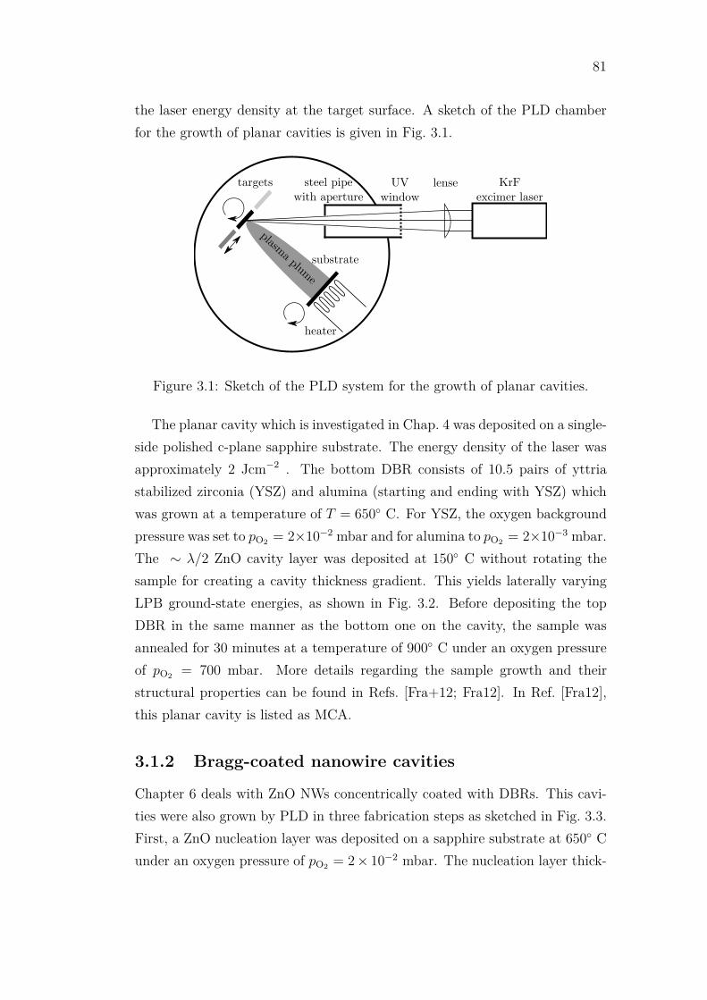
81

the laser energy density at the target surface. A sketch of the PLD chamber

for the growth of planar cavities is given in Fig. 3.1.

UV

window

lense KrF

excimer laser

steel pipe

with aperture

targets

substrate

heater

plasma plum

e

Figure 3.1: Sketch of the PLD system for the growth of planar cavities.

The planar cavity which is investigated in Chap. 4 was deposited on a single-

side polished c-plane sapphire substrate. The energy density of the laser was

approximately 2 Jcm−2 . The bottom DBR consists of 10.5 pairs of yttria

stabilized zirconia (YSZ) and alumina (starting and ending with YSZ) which

was grown at a temperature of T = 650 C. For YSZ, the oxygen background

pressure was set to pO2= 2×10−2 mbar and for alumina to pO2

= 2×10−3 mbar.

The ∼ λ/2 ZnO cavity layer was deposited at 150 C without rotating the

sample for creating a cavity thickness gradient. This yields laterally varying

LPB ground-state energies, as shown in Fig. 3.2. Before depositing the top

DBR in the same manner as the bottom one on the cavity, the sample was

annealed for 30 minutes at a temperature of 900 C under an oxygen pressure

of pO2= 700 mbar. More details regarding the sample growth and their

structural properties can be found in Refs. [Fra+12; Fra12]. In Ref. [Fra12],

this planar cavity is listed as MCA.

3.1.2 Bragg-coated nanowire cavities

Chapter 6 deals with ZnO NWs concentrically coated with DBRs. This cavi-

ties were also grown by PLD in three fabrication steps as sketched in Fig. 3.3.

First, a ZnO nucleation layer was deposited on a sapphire substrate at 650 C

under an oxygen pressure of pO2= 2 × 10−2 mbar. The nucleation layer thick-

82

68 70 72 74 76 78 80

36

38

40

42

44

46

48

y (m

m)

x (mm)

3.290

3.305

3.320

3.335

3.350

3.365

Energy (eV

)

Figure 3.2: PL mapping at T = 10 K revealing spatially varying LPB ground-

state energy as a consequence of the thickness-gradient of the ZnO cavity layer.

Adapted from Ref. [Fra12].

ness is responsible for the resulting area density of the subsequently grown

NWs. The nucleation layer was grown in a second PLD step under low vac-

uum conditions and under argon atmosphere (pAr = 100 mbar) at T = 600 C

as described in [Cao+09]. The nanowire density has to be chosen such that

mutual shadowing is inhibited during the deposition of the DBR with oblique

incidence PLD in a third PLD step. During the oblique incidence deposition,

the sample was rotated around the wire axis to guarantee radial symmetric

DBR layers. Also these DBRs consist of 10.5 layer pairs of YSZ and alu-

mina. A detailed description of the NW and radial DBR growth is given in

Ref. [Sch+10].

83

Figure 3.3: PLD growth steps of nanowire cavities including gas pressure and

temperature. Left: ZnO nucleation layer. Middle: nanowires. Right: DBR

deposition. Adapted from Ref. [Sch+10].

3.1.3 Microwire cavities

3.1.3.1 Bare microwires

Chapter 5 deals with hexagonal ZnO MWs acting as microcavities. The ZnO

MWs were grown by carbothermal vapor phase transport (VPT) by M. Wille

and C. P. Dietrich at the Universität Leipzig. A pressed target pellet consisting

of zinc oxide and carbon in a mass ratio of 1:1 was put in a tube furnace and

heated up to 1400 K with a temperature ramp of 300 K/h. The temperature

was then kept constant for 1 h, before cooling down with 300 K/h. The growth

process took place in ambient air and can be described as a simultaneous

oxidation and reduction of carbon and zinc [Die12]:

C(s) + 2 ZnO(s) −−→ CO2(g) + 2 Zn

C(s) + ZnO(s) −−→ CO(g) + Zn(g).

Here, the letters in brackets represent the solid (s) and gas (g) phase. The

MWs with diameters in the µm range and lengths up to several mm grew di-

rectly on the target pellet in hedge-hoc like structures, as shown in Fig. 3.4.

After the growth process, the MWs have been transferred onto sapphire sub-

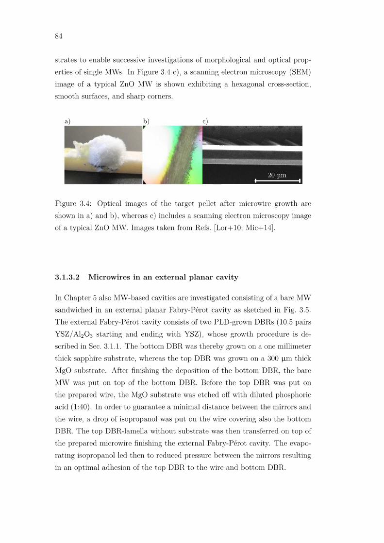
84

strates to enable successive investigations of morphological and optical prop-

erties of single MWs. In Figure 3.4 c), a scanning electron microscopy (SEM)

image of a typical ZnO MW is shown exhibiting a hexagonal cross-section,

smooth surfaces, and sharp corners.

Figure 3.4: Optical images of the target pellet after microwire growth are

shown in a) and b), whereas c) includes a scanning electron microscopy image

of a typical ZnO MW. Images taken from Refs. [Lor+10; Mic+14].

3.1.3.2 Microwires in an external planar cavity

In Chapter 5 also MW-based cavities are investigated consisting of a bare MW

sandwiched in an external planar Fabry-Pérot cavity as sketched in Fig. 3.5.

The external Fabry-Pérot cavity consists of two PLD-grown DBRs (10.5 pairs

YSZ/Al2O3 starting and ending with YSZ), whose growth procedure is de-

scribed in Sec. 3.1.1. The bottom DBR was thereby grown on a one millimeter

thick sapphire substrate, whereas the top DBR was grown on a 300 µm thick

MgO substrate. After finishing the deposition of the bottom DBR, the bare

MW was put on top of the bottom DBR. Before the top DBR was put on

the prepared wire, the MgO substrate was etched off with diluted phosphoric

acid (1:40). In order to guarantee a minimal distance between the mirrors and

the wire, a drop of isopropanol was put on the wire covering also the bottom

DBR. The top DBR-lamella without substrate was then transferred on top of

the prepared microwire finishing the external Fabry-Pérot cavity. The evapo-

rating isopropanol led then to reduced pressure between the mirrors resulting

in an optimal adhesion of the top DBR to the wire and bottom DBR.

85

Figure 3.5: Cross sectional sketch of a ZnO MW being placed in an external

planar Fabry-Pérot cavity.

3.2 Spectroscopy

In this section the spectroscopic methods of photoluminescence (PL) and reflec-

tivity measurements in combination Fourier-imaging methods are introduced.

It is explained, how these techniques are implemented in a micro-imaging setup

in the semiconductor physics group at the Universität Leipzig.

3.2.1 Photoluminescence measurements

Photoluminescence (PL) is a versatile tool to probe the occupation of elec-

tronic and excitonic states. Standard PL uses single photon absorption of

photons with an energy larger than the energy of the electronic transitions

being probed. If the photon is absorbed by an electron, the electron is trans-

ferred in an excited state. This excited state in general has a finite lifetime as

the presence of perturbations leads to a finite decay rate [LL65]. Two promi-

nent perturbations are virtual photons representing vacuum fluctuations and

real photons. The presence of virtual photons leads to the so called spon-

taneous emission rate according to Fermi’s golden rule [Gru06]. Here, the

electron decays into a lower energy state under emission of a photon with the

respective energy distance. An important characteristic of the spontaneous

emission is that the emitted photons have no fixed phase correlation although

the electrons are excited coherently by the laser light. In contrast to that,

86

transition energy (eV)

EX,A 3.377

EX,B 3.382

EX,C 3.426

D0X 3.361

Table 3.2: Important excitonic transitions at T = 10 K as given in

Ref. [Mey+04]. EX,i (i=A,B,C) denote the free excitons. D0X belongs to defect

bound exciton related to alumina.

the presence of a real photon matching a possible electronic transition energy

can induce with a certain probability the emission of a second photon, whose

energy, phase, polarization, and momentum equals that of the incoming pho-

ton [Kli12]. This process is called stimulated emission. In addition to the

two particle (electron-photon or exciton-photon) processes described before,

also three particle interactions can be detected via PL. Especially in ZnO, the

room-temperature PL signal is dominated by phonon-replica of the exciton-

polariton states resulting from the lowest energy excitons [Sha+05; Vos+06].

Thereby, the exciton-polariton decays under emission of a photon and a longi-

tudinal optical phonon. The detectable photon carries the difference in energy

of the two other (quasi)-particles.

Independent of the emission process being stimulated or spontaneous, the

emitted photons carry the information about energy and occupation of the

dipole allowed electronic states of the system which are analyzed by the de-

tection setup.

In Figure 3.6 a), the low temperature PL spectra of c-orientated ZnO are

plotted which are dominated by the emission from defect bound excitons, free

excitons and their corresponding phonon replica. In Table 3.2, important

excitonic transitions in ZnO are listed for T = 10 K.

Excursus: Charge carrier density approximation

In PL experiments with single photon absorption (non-resonant excitation),

the induced carrier density ρ can be approximated by [Kli+07]

ρ =P

A

τ

~ωexcl, (3.1)

where P is the pulse power for pulsed or continuous wave (CW) power for CW-

87

Figure 3.6: In a), low-temperature PL spectra of c-oriented bulk ZnO and of a

ZnO thin film sample are shown (adapted from Ref. [EKR08]) in the spectral

vicinity of the band gap. They are dominated by the emission from defect-

bound excitons and their corresponding phonon replica. A low-temperature

reflectivity spectrum of c-orientated bulk-ZnO in the spectral vicinity of the

band gap is shown in b) (adapted from Ref. [Sha+05]). The reflectivity spec-

trum is dominated by reflection peaks being connected to the lowest energy

(n = 1) states of the free A- and B-exciton resonances.

88

short pulse long pulse

(Texc < 300 ps) (Texc ≥ 300 ps)

thin samplePP

ATexc

~ωexcdPP

A300 ps~ωexcd(50 nm < d < 1 µm)

thick sample(d ≥ 1 µm)PP

ATexc

~ωexc1 µmPP

A300 ps

~ωexc1 µm(d ≥ 1 µm)

Table 3.3: Formulae for the calculation of the carrier density ρ for PL exper-

iments at ZnO samples for non-resonant excitation above the band gap. The

different quantities are explained in the main body of the text.

experiments, A the excited area2 on the sample surface and ~ωexc the photon

energy of the excitation laser beam. The characteristic length l is for samples

thicker than the penetration depth of the laser (typically 50 nm) given by the

carrier diffusion length lD (typically 1−3µm in ZnO) or by the sample thickness

d if d < lD. The characteristic time τ depends on the lifetime T1 of the excited

electron-hole pairs with respect to the temporal length of the excitation pulse

Texc. The typical lifetime for excitons in ZnO is 300 ps [Kli+07]. Therefore,

for nano- and femtosecond pulses, the created carrier density is resulting from

τ = Texc whereas τ = T1 yields reasonable results in the case of nanosecond

or longer pulses. For the carrier density ρ, this leads to four cases as listed in

Tab. 3.3 which play a role within this thesis. This considerations imply that

for short-pulse excitation the quantity of a photon energy density I = PTexc/A

is proportional to the generated charge carrier density, whereas for long-pulse

or CW-excitation the power density P/A is proportional to ρ.

3.2.2 Reflectivity measurements

3.2.2.1 Reflectometry

In contrast to PL experiments, the density of states is probed in reflection

measurements. In addition, the reflectivity spectrum of a sample can also give

access to the sample geometry. The DF of the sample can be obtained by

2A discussion on the power density in the center of a focused Gaussian beam and how

this quantity is experimentally obtained, can be found in Sec. 3.2.5.

89

modeling reflectivity spectra as the reflectivity under normal incidence at the

interface to vacuum is given for isotropic materials by:

R(E) = |r(E)|2 =(n(E) − 1)2 + κ(E)2

(n(E) + 1)2 + κ(E)2, (3.2)

again with√ǫ(E) =

√ǫ1(E) + iǫ2(E) ≡ n(E) + iκ(E). If the material is

uniaxial with its optic axis situated in the surface plane, Eq. (3.2) can only

be used if a polarizer selects the fields perpendicular or parallel to the optic

axis. Modeling these polarization-resolved reflectivity spectra yields ǫ‖ and

ǫ⊥, respectively. Excitonic contributions to the DF ǫ are modeled by Lorentz-

oscillators as already introduced by Eq. (2.37). The contribution of exciton-

phonon complexes (EPC) to the imaginary part of the DF is important to

correctly describe the DF in the spectral vicinity of the band gap [Neu15].

The contribution of EPC is modeled by weighted replica of the zero phonon

resonance (ǫX2 ) of the corresponding exciton shifted by an integer number m

of the mean phonon energy ELO [Sho+08]:

ǫEPC2 = f0

∑

m

bm−1ǫX2 (E −mELO). (3.3)

Here, f0 describes the exciton-phonon coupling constant and bm−1 the proba-

bility of occurrence of the m-th phonon state. Band-to-band transitions near

the fundamental band gap in direct-band gap semiconductors can be modeled

with 3DM0-crtical point structures given by [EKR08]:

ǫ3DM0 =∑

α

Aα0 (Eα

0 )−3/2

(2 − (1 + χα

0 )1/2 − (1 − χα0 )1/2

(χα0 )2

), (3.4)

with

χα0 = (E + iΓ0/E

α0 ). (3.5)

The quantities Aα0 and Eα

0 represent the amplitude and transition energy of

the critical point.

Within reflectivity experiments, a measured reflectivity spectrum Imeas(E)

is the product of the real reflectivity R(E) of the sample and a setup function

G(E):

Imeas(E) = R(E)G(E). (3.6)

Therefore, a reference sample with an already known reflectivity Rref has to

be measured under the same conditions as the sample of interest in order to

90

obtain the setup function:

Iref(E) = Rref(E)G(E), (3.7)

with Iref(E) being the measured (bare) reflectivity of the reference sample.

The real reflectivity of the sample is then given by:

R(E) = Imeas(E)Rref(E)Iref(E)

(3.8)

For reflectivity measurements presented in this thesis, a silicon single crystal

was used as reference. Rref was obtained by modeling spectroscopic ellipsom-

etry data (see Sec. 3.2.2.2).

3.2.2.2 Spectroscopic ellipsometry

As a special form of reflectometry, spectroscopic ellipsometry (SE) measures

the change in the polarization state of light during reflection (or transmission)

at or through a sample, respectively [Fuj07]. This allows to determine layer

thicknesses and DFs of thin films by modeling the experimentally measured

data. A great advantage in comparison to standard reflectivity measurements

is that there is no need for a reference measurement as intensity ratios are

measured instead of intensities. Therefore, SE is also less sensitive to intensity

fluctuations. The change of the polarization state can be expressed by the

quotient of the complex reflexion coefficients rp and rs due the ellipsometrical

quantities Ψ and ∆:

ρ =rp

rs

= tan Ψ exp i(∆p − ∆s) = tan Ψ exp i∆. (3.9)

This expression is only valid for isotropic media or uniaxial ones with the

optical axis aligned to the normal of the sample surface. Otherwise the more

complex Müller matrix formalism has to be applied.

3.2.3 Time-resolved measurements

In order to measure the radiative decay rate or life time of excited electronic

states, it is convenient to perform time-resolved PL measurements. Therefore,

a temporally short laser pulse excites electrons and the emitted photons per

91

unit time are counted in dependence on the temporal distance after the ex-

citation pulse. For this purpose, a streak camera was used. In Figure 3.7,

the basic working principle of a streak camera is sketched. The streak camera

possesses a horizontal entrance slit along which spatial informations can be

encoded with the incoming optical signal. These incoming photons generate

photo-electrons proportional to the number of initial photons at a photo cath-

ode. An accelerating mesh is placed behind it. There, a horizontal electric field

accelerates the photo-electrons towards two deflector plates, where a sawtooth

voltage is applied resulting in a temporal varying vertical deflection. This

means that electrons arriving later at the streak camera entrance are deflected

more strongly. After passing the deflector plates, the photo-electrons hit a

multi-channel plate (MCP) where their number is multiplied several times be-

fore hitting a phosphor screen. The fluorescence of this screen is proportional

to the intensity of the original incoming signal and is filmed with an array

CCD. In the vertical direction of the CCD, the temporal information of the

incoming signal is encoded, whereas in the horizontal direction a spatial in-

formation can be recorded. By placing a spectrometer in front of the streak

camera entrance slit, the spatial information can be transferred into a spectral

information of the incoming photons.

light

intensity

timespace

slit photocathode

lenses

sweep circuit

trigger signal

MCP phosphor

screen

sweep

electrode

streak image on

phosphor screen

time

space

accelerating

mesh

Figure 3.7: Schema of the basic units of a streak camera. Adapted

from Ref. [Ham10].

92

3.2.4 Coherence measurements

For the characterization of light emitted from a sample regarding its coherence

properties, a Michelson interferometer was placed in the collimated beam be-

tween the objective and the image forming lens in front of the detector. The in-

terferometer setup was planned, built and characterized by M. Thunert [Thu17].

The configuration which was used for the measurements within this thesis in-

cluded a retro-reflector (RR) in one arm of the interferometer whereas the

other arm was equipped with a plane mirror (PM). The RR was used to invert

the image of the sample surface in one arm of the interferometer. This con-

figuration enables probing the first order spatial coherence function g1(~x,−~x)

yielding g1(~x,−~x) = 1 for totally coherent signals and g1(~x,−~x) = 0 for inco-

herent signals. Here, ~x is a position vector in the plane of the sample surface

whose origin (~x = 0) is the inversion center. Typically, the inversion center

is superimposed with the excitation center in PL-experiments. The length of

both interferometer arms was equalized in order to separate spatial coherence

effects from temporal ones. This was done by overlapping the images of two

150 fs long laser pulses generated from one pulse by the beam splitter (BS) of

the interferometer. This allows to equalize the arm lengths within a range of

about 20 µm.

In order to extract g1(~x,−~x) from a measured interference pattern one has

to get rid of intensity differences (I1(~x)-I2(−~x)) which are either produced

by the sample itself or by transmission or reflection differences occurring in

the arms of the interferometer. This can only be done if in addition to the

interference pattern Iinterf(~x,−~x), also the single arm intensity patterns, I1(~x)

and I2(−~x), are recorded separately. A normalized interference pattern which

is independent of the intensity deviations in the single arms can be calculated

via [Kav+07]:

Inorm(~x) =Iinterf(~x,−~x) − I1(~x) − I2(−~x)

2√I1(~x)I2(−~x)

= g1(~x,−~x) cos (~kinterf~x+ φ).

(3.10)

The quantities ~kinterf and φ describe the setup-defined interference wave vec-

tor and phase. The amplitude of the interference fringes of the normalized

intensity gives the first order spatial coherence function g1(~x,−~x).

93

3.2.5 Micro imaging setup

Figure 3.8: Schema of the micro imaging setup.

The micro imaging setup in the semiconductor physics group at the Uni-

versität Leipzig is a versatile tool for spectroscopy with µm spatial resolution.

It was initially built by T. Nobis and C. Czekalla as a fiber based system.

A further improvement of the setup regarding time-resolved measurements in

combination with real and momentum space imaging, was initiated by the au-

thor of this thesis within his master thesis [Mic12]. The implementation of

an interferometer was done by M. Thunert within his PHD thesis [Thu17]. A

sketch of the setup as being present during the time, when the measurements

for this thesis where done, is given in Fig. 3.8. The available light sources are

on the one hand classical light sources (neon or xenon lamps) for the generation

of a broadband and continuous wave (cw) signal which is used for reflectivity

measurements. On the other hand, several laser sources (pulsed and cw) are

94

source pulse energy wavelength(s) rep. rate pulse width

HeCd cw 325 nm - -

Ti:Sa 1 nJ 233-300 nm 0.03-76 MHz 150 fs/2 ps

10 nJ 350-450 nm 0.03-76 MHz 150 fs/2 ps

50 nJ 700-900 nm 0.03-76 MHz 150 fs/2 ps

Nd:YAG 1/3/50 µJ 266/355/532 nm 0-100 kHz 5 ns

Nd:YAG 2 mJ 266 nm 20 Hz 10 ns

Nd:YAG cw 266 nm - -

Table 3.4: List of laser light sources available for PL experiments including

important emission properties.

available for PL excitation. Table 3.4 includes the different laser light sources

used for this thesis and their most important emission properties. Typically,

the light beam of the source of choice is focused on a pinhole before being

collimated and sent via a beam splitter to the back entrance pupil of the mi-

croscope objective. The reflected or generated optical signal is captured by the

same objective. Two main modi for the detection of the signal of interest are

possible: real space or angular-resolved imaging. For imaging the real space

emission (or reflectivity) in the simplest case, a second lens L2 behind the ob-

jective images the object plane on the spectrometer entrance slit or directly on

a CCD camera. The second modus is the angular-resolved or k-space imaging

modus. Here, the Fourier plane of the objective is imaged with the lenses L1

and L2 on the spectrometer entrance slit (or CCD) as sketched in Fig. 3.9 b).

The spectrometer is either coupled to a streak camera setup for time-resolved

measurements or directly to an array CCD. This setup in principle allows for

the measurement of the time-, space-, energy- and angle-dependence of an op-

tical signal. For coherence measurements, a Michelson-interferometer is placed

in the collimated beam behind the objective. In the case of real space mea-

surements, the interferometer is placed between the objective and the image

forming lens L2. In the case of k-space imaging it has to be placed between

L1 and L2 in order to be in the collimated beam with respect to Fourier plane

of the objective. More details about the theory of Fourier-imaging techniques

can be found in Ref. [Hec05] and in Appendix A.5. For the reconstruction of

95

spatial, spectral, and temporal informations from the sample surface, image

forming lens L2 was implemented in an automatized X-Y scanning stage.

Figure 3.9: Sketches of the real and k-space detection setup lens alignment are

shown in a) and b), respectively.

Excursus: Spatial resolution and focus spot width

In order to quantify the quality of an obtained image, it is important to

determine the spatial resolution of the actual setup. For spatially resolved PL-

measurements, where the light of a laser beam is focused on a sample surface

and the generated PL-signal and/or the reflected light of the laser beam is

imaged on a monochromator entrance slit, one can determine the resolution

directly by illuminating surface irregularities which are smaller than the actual

resolution of the setup and measure their spatial extension from the image. For

PL measurements it would be optimal to excite single separated quantum dots

and detect their emission as a point spread function.

In contrast to that if the momentum or k-space is imaged then a spatially

resolved image is not directly given. Here, it is important to know the spatial

extent of the excitation source (white light or laser spot) on the sample surface.

96

Figure 3.10: Schema of the knife-edge method for the determination of the

focus spot size.

Therefore, it is useful to scan a sharp edge through the focal plane which

successively shadows, reflects or transmits the focused light. Within this thesis,

always a reflection geometry was used to measure the spot size with this so

called knife-edge method. The working principle is sketched in Fig. 3.10 with a

cleaved Si-substrate used as a reflecting sample whose edge is scanned through

the focus. If a circular symmetrical and Gaussian-shaped focus is assumed,

the intensity distribution can be written as:

I(x, y) = I0e− ln 2(x

r )2

e− ln 2( y

r )2

, (3.11)

with I0 being the intensity in the center of the focus spot and r being the

radius where the intensity drops to I0/2. The integrated total intensity is then

given by:

Ptot,Gauss = I0

∫ ∞

−∞e− ln 2(x

r )2

dx∫ ∞

−∞e− ln 2( y

r )2

dy = I0π

ln 2r2. (3.12)

If a reflecting substrate with a sharp edge is pulled in x-direction out of the

focus spot as sketched in Fig. 3.10 the measured integrated intensity at the

position x = x0 is given by:

P (x0) = Ptot,Gauss − I0

√π

ln 2r∫ x0

−∞e− ln 2(x

r )2

dx

=Ptot,Gauss

2

(1 − erf

(x0

√ln 2r

)).

(3.13)

In Fig. 3.11 a) a Gaussian distribution is plotted together with the correspond-

ing knife-edge signal P (x0).

For high excitation density PL experiments it is crucial to obtain the ex-

perimentally present power (or energy) density in the center of the Gaussian

97

excitation beam at the sample surface. This is necessary in order to estimate

the generated carrier density (see. Sec. 3.2.1). The maximum power (or en-

ergy) density can be obtained if the Gaussian beam distribution is compared

with a so called top hat distribution with the same maximum and integrated

total intensity Ptot,th as sketched in Fig. 3.11 b). Mathematically, this com-

parison reads:

Ptot,Gauss = Ptot,th (3.14)

I0

√π

ln 2r2 = I0πr

2th, (3.15)

and yields for the dependency of the different radii:

rth =r√ln 2

≈ 1.2r. (3.16)

So if the total power Wmeas (or energy) of a beam is known, the power (or

energy) density Pmeas in the center of the Gaussian beam can be calculated

via:

Pmeas =Wmeas

πr2th

=Wmeas

1.44πr2. (3.17)

-4 -3 -2 -1 0 1 2 3 4

0.0

0.5

1.0

-4 -3 -2 -1 0 1 2 3 4

0.0

0.5

1.0 Gaussian Signal

P/P

0 I/

I 0

x0/r

2r

Gauss. top hat

I/I 0

x0/r

rth 1.2r

Figure 3.11: a) Gaussian beam intensity distribution (gray) with radius r

(HWHM) and corresponding knife-edge signal (black). In b) a top hat distribu-

tion with radius rth is plotted, whose total integrated and maximum intensity

corresponds to that of a Gaussian distribution.

Part II

Experimental Results

99

101

The experimental results of this thesis are separated in three chapters:

• Chapter 4 deals with exciton-polaritons in a planar microcavity (MC)

consisting of an active ZnO layer being situated between two plan-parallel

distributed Bragg reflectors (DBRs). Therein, polaritons are confined

along one spatial direction and are able to propagate freely within the

plane of the cavity. In such a MC, acceleration and relaxation processes

of exciton-polaritons in a spatially varying potential are investigated. It

is shown that the theoretical model derived for condensed polaritons also

holds for polaritons in the uncondensed phase. A scattering constant is

deduced describing the relaxation processes in both phases.

• One possibility to circumvent the growth of multilayer DBRs while keep-

ing a high quality factor of the cavity modes, is to use total internal

reflection (TIR) for photonic confinement. Self-assembled grown ZnO

microwires (MWs) represent, due to their hexagonal cross-section, high

quality cavities as light is reflected six times by TIR forming a closed

path. Naturally in this kind of cavity, photons (polaritons) are con-

fined in two spatial dimensions and their spatial overlap with the ZnO-

exciton states is close to one. Along the wire axis, the resulting WGM-

polaritons are able to propagate freely. Therefore, Chap. 5 deals with

exciton-polaritons in this MW cavities. There, it is shown that the pro-

cess of polariton-phonon scattering enables room temperature lasing in

homogenously pumped high quality MW cavities. In contrast to that,

it is demonstrated that a spatially narrow excited electron-hole-plasma

(EHP) acts as a small perturbation and source for the strongly coupled

polaritons. The obtained results, namely modal blue-shift, threshold

behavior in intensity and linewidth, condensation in momentum space,

long-range spatial coherence, and repulsive polariton-polariton interac-

tion resulting in ballistic propagation, show the typical characteristics be-

ing usually connected to a driven-dissipative polariton Bose-Einstein con-

densate. The spectral appearance of these coherent states in momentum-

and real space is typically modeled with a mean field theory based

on solving a Gross-Pitaevskii equation. But these effects can also be

explained from resonant modes propagating in a cavity with spatially

102

varying dielectric function as a consequence of the locally pump-altered

charge carrier density.

In order to reduce surface-connected losses, hexagonal ZnO microwires

are placed in external planar Fabry-Pérot (FP) cavities. Such hybrid

cavities exhibit vastly increased quality factors of the WGM-like polari-

ton branches and enable reduced lasing thresholds of up to a factor of

two.

• Within Chapter 6, the border between two- and three-dimensional con-

finement is traced out. There, it is shown how ZnO nanowires, which are

in general too thin for a good lateral photonic confinement, are coated

with radial DBRs to achieve a sufficient lateral confinement for the for-

mation of exciton-polaritons. The special design of this cavity structure

allows for the simultaneous appearance of the weak and strong coupling

regime. At low temperatures, the high crystal quality of the ZnO NWs

enables the observation of middle polariton branches emerging in the

free spectral range between the excitonic A- and B-ground-states. The

obtained results and interpretations are supported by FDTD simula-

tions, which were performed by R. Buschlinger at the Friedrich-Schiller-

Universität Jena. Finally, EHP-related lasing is demonstrated in these

kinds of cavities up to room temperature.

Chapter 4

Results I: Polariton relaxation

in an inhomogenous potential

In the first results-part of this thesis, acceleration- and relaxation-processes are

investigated for polariton populations in an inhomogenous potential within a

planar cavity. This is done for two distinct situations: the coherent phase

beyond the nonlinear density threshold and the incoherent phase.

From various experiments with planar and wire-like microcavities (MCs),

it is well known that a pump-induced spatially inhomogenous background po-

tential can lead to nearly equally spaced energy levels in the momentum space

distribution for coherent bosonic quantum fluids beyond the nonlinear density

threshold [Chr+07; Kri+09; Wer+10; Gui+11; Fra+12]. It is shown here that

this particular pattern is also observable for exciton-polaritons far below the

critical density and the theoretical model developed for polariton condensates

turns out to be applicable without further modifications.

4.1 Experimental and sample details

The ZnO-based microcavity under investigation is the same as has been de-

scribed in detail in Ref. [Fra+12] and whose fabrication is described in Sec. 3.1.1.

In order to calculate bare cavity modes, the dielectric function (DF) of the ZnO

cavity layer has to be known. Therefore, ellipsometric measurements have

been performed on the sample, before the top Bragg mirror was deposited. In

Fig. 4.1 b), the modeled complex refractive index of the ZnO cavity layer is

103

104

plotted with and without excitonic contributions for T = 10 K. The A- and B-

exciton ground-states cannot be identified independently which is a result of

the structural disorder in the ZnO cavity layer [Thu+16]. This layer consists

of c-orientated crystallites with a maximum tilt of ±12 which is confirmed

by X-ray diffraction measurements, as shown in Fig. 4.1 a). The microcavity

shows nonlinear emission behavior if the excitation power density exceeds a

certain threshold. The specific threshold behavior in dependence on detuning

and temperature is intensively investigated in Refs. [Fra+12; Fra12]. Further-

more, the nonlinear threshold is accompanied with the evolution of coherent

polariton states as described in Ref. [Thu+16].

Figure 4.1: In a), the transmission electron microscopy image (bright-field) of

the half planar microcavity structure is plotted revealing a textured structure

and columnar growth of the ZnO-cavity layer. The inset in a) shows the diffrac-

tion pattern which was taken from the encircled region enabling the determina-

tion of the tilt of the ZnO crystallites. The image is taken from Ref. [Fra+12].

In b), the complex index of refraction of the ZnO cavity layer with (solid) and

without (dashed) excitonic contributions is plotted. The refractive index n

(black) and extinction coefficient κ (gray) are shown in the spectral vicinity

of the excitonic ground-states at T = 10 K for polarization perpendicular to

the optic axis of ZnO. A- and B-excitonic ground-states are not separable and

appear as one peak at EX,A/B = 3.378 eV. Adapted from Ref. [Stu+09].

The excitation conditions for the results presented in this section have been

chosen differently as in Refs. [Fra+12; Fra12]. For single photon excitation

105

above the band gap, frequency-tripled light of a mode-locked laser (titanium-

sapphire) was used with a wavelength of λ = 266 nm. The repetition rate was

76 MHz and the pulse width 2 ps. The laser beam was focused to an area of 5

µm2 with an UV objective (magnification 50×, numerical apertur 0.4) with a

detectable angular range of ±23. The detection of the light reflected or emit-

ted from the sample was realized in a confocal configuration, as described in

Sec. 3.2.5. The lens setup allows for the real space as well as of the momentum

or k-space, as shown in Fig. 3.9. For the investigation of relaxation processes

taking place in the spatial region where the pump-induced background poten-

tial is strongly inhomogenous, a pinhole (PH) was installed in an intermediate

image plane, such, that only the PL signal emitted from the central excitation

area of 3 µm2 was detected. This is shown exemplarily in Fig. 4.2.

20 25 30 35 40 45 50110

115

120

125

130

135

140

y (µm

)

20 25 30 35 40 45 50

① ①

0.0 0.5 1.0 0.0 0.5 1.0

Norm. PL intensity Norm. PL intensity

Figure 4.2: Spatially resolved polariton emission beyond the nonlinear thresh-

old: without a) and with b) the use of a pinhole in an intermediate image

plane restricting the detection area.

4.2 Experimental results

The results which will be presented below were obtained at a sample position

corresponding to a detuning of δ = −30 meV between the excitonic A/B

106

complex and the bare cavity mode ground state at T = 10 K. Figure 4.3 a)

shows the lower polariton branch (LPB) emission below the nonlinear threshold

without PH and includes the dispersion relations of the uncoupled exciton

(EX,A/B) and of the calculated bare cavity-photon mode (EC) [Stu+11a]. The

broadening (HWHM) of the LPB is measured to be γuncoh = (1.4 ± 0.2) meV.

Figure 4.3: Energy-resolved k-space image of the LPB for δ = −30 meV below

(0.04 Pth; a) and above (1.6 Pth; b) the nonlinear threshold. The modeled

LPB dispersion is plotted as a white line. The modeled uncoupled exciton

and cavity-photon dispersion are marked with EX,A/B and EC, respectively.

In c), the PL spectrum at k‖ = 0 µm−1 from the marked region in b) is

shown. ∆Er,coh marks the energy spacing between consecutive dispersionless

LPB states appearing beyond the threshold. In order to quantify the exact

spectral position of these states, the measured data (black symbols) were mod-

eled with Voigt oscillators (gray lines). All experimental data were acquired

at T = 10 K.

Above the nonlinear threshold, as shown in Fig. 4.3 b) and c), several dis-

persionless states appear bounded by the dispersion relation of the low den-

sity LPB. These states are nearly equally spaced in energy (see Fig. 4.3 c)

with a distance of ∆Er,coh = (1.7 ± 0.3) meV and a broadening of γcoh =

(0.75 ± 0.2) meV (see also Refs. [Fra12; Fra+12]). Thus, one can conclude

that the lifetime of the polariton states above threshold is roughly twice as

high as for polaritons below threshold. It should be noted that the spectral

broadening of the states beyond the threshold, as shown in Fig. 4.3 b) and

c), is increased additionally to the lifetime broadening by temporal potential

reduction caused by the short Ti:Sa pump-laser pulses [ST12] which is demon-

107

strated in Fig. 4.4. The 2 ps short pump pulse induces a carrier density which

has a temporal maximum (at about 15 ps in Fig. 4.4 b) which is connected

to the highest potential energy. At this point in time, the temporal change

of the carrier density vanishes (dn/dt = 0) and a temporally short equilib-

rium is established. At this time, the higher energy states are present. Then,

with decreasing reservoir carrier concentration in time, also the background

potential shrinks accompanied by a reduction of the energy of all polariton

states and a vanishing of the higher energy states. To exclude these distort-

ing effects induced by short excitation pulses, the broadening of the polariton

states beyond threshold was determined from PL spectra obtained from ex-

periments presented in Refs. [Fra+12; Fra12] with a diode laser exhibiting a

pulse duration of 500 ps1 acting as quasi continuous excitation source yielding

spectrally narrow polariton states above threshold in time-integrated measure-

ments. The lowest energy state at 3.320 eV is excluded in Fig. 4.3 c) because

of its strong inhomogenous broadening being introduced by the relatively long

effective lifetime of this state, whose energy decreases according to the decreas-

ing background potential (see Fig. 4.4 b).

Regarding the k-space emission pattern for increasing excitation power den-

sities, the situation changes drastically if only photons are collected being emit-

ted from the central excitation area. There, the pump-generated background

potential is strongly inhomogenous. This is shown in Fig. 4.5, where one

can clearly see that in addition to the dominating LPB, two further polariton

branches are present at higher energies even far below the nonlinear threshold.

If the PH is used for spatial filtering, as shown in Fig. 4.5, the LPB emission

is smeared out and broadened. This is connected to the Heisenberg princi-

plem which states that momentum and position cannot be exactly measured

simultaneously: ∆x∆k ≥ 0.5. Furthermore, the detectability of high-k|| sates

is suppressed as the cryostat window introduces aberrations strongly increas-

ing with the emission angle (∝ k‖) which causes the according photons to be

blocked at the PH [Mic12]. Note that for increasing excitation power density,

the modes are also blue-shifted but the spectral distance between these addi-

tional modes of ∆Er,uncoh = (3.3±0.1) meV remains constant, as demonstrated

more clearly by the k|| = −2 µm−1 spectra in Fig. 4.5 b). These additional

1This excitation laser was not available for the measurements presented in this work.

108

Time (ps)-6 -4 -2 0 2 4 6

30

32

34

36

38

Figure 4.4: Temporal evolution of coherent polariton states: A time-integrated

k-space image above threshold is shown in a) for T = 10 K. The temporal evo-

lution of the k‖ = 0 states from a) is shown in b). The brightest state (dashed

line) red shifts about 3 meV in the observable time range as a consequence of

the temporally decreasing background potential. The sample position probed

here, is a similar one as in Fig. 4.3.

LPB branches are not symmetrical to k|| = 0 µm−1 because of the laser spot

shape being not rotationally symmetric, as shown in Fig. 4.7 a). This is a

consequence of the birefringent frequency tripling crystals. At high excitation

power densities (10 Pth in Fig. 4.5 a) and 4.5 b), the bare cavity-photon mode

EC is supposed to become visible as the mean charge carrier density in the

observed spatial region of the cavity may reach the Mott density, which is

accompanied by the disappearance of the lasing emission from the LPB states.

As stated before, at the nonlinear threshold dispersionless states emerge in

the energy-resolved k-space images which are nearly equally spaced in energy.

These states represent the coherent emission of LPB staes [Thu+16] which are

expelled from the highly excited area [Wer+10; WCC08] and energetically relax

in the decreasing background potential when leaving the central excitation

area. The appearance of these states above the nonlinear threshold has been

observed also by other groups [Wer+10; Gui+11; Chr+07; Kri+09] and was

explained in Refs. [WCC08; WLS10] as a consequence of the dynamical balance

109

of in- and outscattering rates for bosonic states of different energy [WLS10].

The balance criterion states:

Γin = Γout. (4.1)

Following Wouters et al. [WLS10], the inscattering rate Γin for a polaritonic (or

bosonic) state is assumed to be proportional to the energy distance between

the actual and the initial state of the scattering process:

Γin = ζ × ∆Er. (4.2)

Here, the scattering constant ζ has the unit of an inverse action and is, for

simplicity, not normalized to an unit density as introduced by Wouters et

al. [WCC08]. The outscattering rate Γout of a polariton state is assumed to

be determined by its radiative lifetime and is therefore proportional to the

homogenous spectral broadening γ (HWHM):

Γout ≃ γ

~. (4.3)

This implies that for states with a doubled spectral broadening (∝ doubled

outscattering Γ), the energetical distance ∆Er to the next stable state has to

be twice as high in order to fulfill the compensation of in- and outscattering

rates, as it is given by Eqs. (4.1) and (4.2). Exactly this is the case within

the experimental observations presented here if the emission of the coherent

polariton states is compared to the emission of the incoherent polariton ensem-

ble, as sketched in Fig. 4.6. From the experimental results we can deduce the

bosonic scattering constant to be ζ = (0.4 ± 0.2) ~−1. This result states that

twice the spectral broadening (HWHM) of a coherent state is roughly the same

as the energy spacing between relaxing coherent states. Similar results were

also observed in Refs. [Gui+11; Chr+07; Wer+10]. The ability of this sim-

ple scattering model to describe both, the coherent and the incoherent phase,

correctly, leads to the conclusion that polariton relaxation within a varying

background potential in both phases can be described with one scattering con-

stant ζ which is independent of the charge carrier or particle density within

the observed range (≥ two orders of magnitude).

The polariton relaxation in the spatially varying potential landscape is con-

nected to an acceleration of the states towards the peripheral region of the

excitation spot as there the local potential energy is smaller. To demonstrate

110

this, the laser spot intensity distribution on the sample surface was recorded

and compared to the emission of the generated incoherent polaritons (see Fig.

4.7). It is obvious that the main emission spots are spatially separated from

the pump spot intensity maximum. Here, one could assume that the incoher-

ent polaritons could be trapped in the spatial region of the first diffraction

minimum of the excitation laser spot (see inset of Fig. 4.7 b). This would pro-

vide another explanation for the appearance of the observed discrete polariton

states a a consequence of quantization in a potential trap created the pump

laser spot’s diffraction pattern. But this explanation is not reasonable as both,

the incoherent and the coherent polaritons, are exposed to roughly the same

trapping potential which would result in equal energy spacings for the trapped

incoherent and coherent polaritons (∆Er,uncoh!= ∆Er,coh). This is obviously

not the case.

Excursus: Repulsive potential

In principle, it is possible to describe the repulsive potential as a consequence

of the charge carrier density-dependent DF of the cavity material as discussed

in Sec. 2.3.1.7. This will be done in the context of WGM-polaritons at room

temperature in Chap. 5. But it has to be mentioned that there is a crucial

difference between a DF which is altered by an increased charge carrier density

(see Fig.2.32), and the DF which is obtained by artificially removing the exci-

tonic contributions, as shown in Fig. 4.1. Example given, for a charge carrier

density-dependent DF many-body interactions lead to the renormalization of

the band gap which is not taken into account, if only the excitonic contributions

are removed from the DF in the zero charge carrier density limit. Unfortu-

nately, for low temperature conditions, as presented here, neither independent

experimental nor theoretical values 2 for the charge carrier density-dependent

DF are known to the author of this thesis. Therefore, a quantitative description

of the occurring phenomena in terms of an charge carrier density-dependent

DF is not possible at this point.

2The model for the charge carrier density-dependent DF used for room temperature [H

H04; Ver+11; Wil+16a] is not valid for low temperatures according to Ref. [Wil+16a].

111

4.3 Summary

This chapter was dedicated to the investigation of polaritons in a planar ZnO-

based microcavity with special attention on their relaxation behavior in a spa-

tially varying potential. Experimental results were shown indicating that the

model of Wouters et al. [WLS10] for relaxation processes describing condensed

polaritons in a spatially varying potential landscape is also valid for polaritons

orders of magnitude below the nonlinear density threshold. This assumption

is supported by k- and real space imaging demonstrating the appearance of

discrete LPB states being roughly equally spaced in energy and furthermore,

an accumulation of polaritons in the peripheral region of the pump-induced

repulsive potential. From the experimental results a value for the bosonic

scattering constant could be deduced.

112

Figure 4.5: In a), the normalized and energy-resolved k-space images for dif-

ferent excitation densities are shown. The dashed black line in the first image

marks the k‖ channel the spectra in b) are taken from. In b), E0 represents

the lowest energy LPB, ∆Er,uncoh marks the energy spacing between two con-

secutive LPB emission states, and EC represents the energy of the bare cavity

mode.

113

Figure 4.6: a) Sketch of the polariton relaxation in a spatially inhomogenous

potential resulting in equally spaced steps in energy. b) Graphical represen-

tation of the compensation of in- and out-scattering rates for coherent and

incoherent polariton states as found experimentally. Adapted from [WLS10]

and modified for the presented case.

0 2 4 6 8 10

0 2 4 6 8 10

0

2

4

6

8

10

②

0 2 4 6 8istance (µm)

Inte

nsi

ty0.0 1.00.5

Norm. PL intensity

Figure 4.7: In a), the real space image of the laser spot on the sample surface

is depicted. The corresponding LPB emission below the nonlinear threshold

is shown in b). The inset in b) shows the normalized intensity profile of the

laser spot (gray) and LPB emission (black) along the dotted lines in a) an b).

Chapter 5

Results II: Polaritons in

hexagonal ZnO microwires

One possibility to circumvent the growth of multilayer mirror systems (as dealt

with in Chap. 4) while keeping high quality factors of the cavity modes is to

use total internal reflection (TIR) for photonic confinement. In this chapter,

self-assembled grown microwire cavities are investigated exhibiting a hexago-

nal cross section leading to high quality factor cavities as photons are reflected

six times by TIR forming a closed round trip. The corresponding modes are

called whispering gallery modes (WGMs) which are intrinsically strongly cou-

pled to the ZnO-exciton ground-states even at room temperature, as shown

in Sec. (2.3.3.4). Naturally, in this kind of cavities polaritons are confined

in two spatial dimensions. The other dimension, along the wire axis, is the

dimension in which the polaritons are able to propagate freely. Furthermore,

the much larger cavity round trip length, compared to planar cavities, gives

access to multilevel-polariton systems incorporating several photonic modes in

the spectral vicinity of the excitonic ground-states.

In the first section of this chapter it is shown that the high quality factors

of the WGMs enable the observation of coherent emission which is triggered

by polariton-phonon scattering in the intermediate density regime. The sec-

ond section of this chapter deals with electron-hole plasma (EHP) induced

polariton-lasing where a small part of the cavity is pumped beyond the Mott

density (high density regime) which ensures that the strong coupling regime

is preserved as the EHP acts only as a perturbation on the polariton states.

115

116

The resulting spatial and temporal evolution of coherent WGM-polaritons are

investigated together with their spatial coherence properties. Furthermore, the

tunability of the lasing energy is demonstrated in combination with switching

between single- and dual-mode operation. This chapter closes with investiga-

tions conducted on hexagonal ZnO microwires being placed in a planar external

FP cavity in order to suppress leaky modes from the wire surface resulting in

vastly increased quality factors.

5.1 Phonon-assisted lasing in ZnO microwires

at room temperature

5.1.1 Experimental and sample details

For the achievement of low lasing thresholds in PL experiments, it is useful to

pump a high ratio of the optical path given by the cavity [Liu+13b; Li+13].

Therefore, a large excitation spot with a diameter of about 150 µm was used

which covered the upper half of the microwire under investigation. The ex-

citation laser pulses had a pulse width of 10 ns at repetition rate of 20 Hz

and a photon energy of 3.66 eV (λ = 266 nm) for non-resonant excitation

above the band gap of ZnO. The microwire was excited under an angle of

about 60 to the wire normal. As the excitation laser beam was not directed

through the microscope-objective, it was not possible to measure the exact ex-

citation spot size with the knife-edge method, as described in Sec. 3.2.5. The

excitation spot size was therefore obtained by imaging of the generated PL

signal of a ZnO single crystal. The non-resonant excitation scheme in general

prevents the transfer of coherence, momentum or polarization into the final

polariton states due to multiple scattering processes with phonons and carri-

ers during relaxation [Kas06; DHY10]. The PL signal of the wire was collected

by the setup which is described in Sec. 3.2.5 enabling spectrally resolved or

two-dimensional real and k-space images. The objective which collected the

PL signal was a Mitutoyo NUV objective with a magnification of 100 and a

numerical aperture (NA) of 0.5 giving access to a detectable angular range of

±30. Within k-space measurements a spatial area with a diameter of 240 µm

was probed, whereas a real space image covers 40 µm in diameter of the object

117

Figure 5.1: In a) a sketch of a hexagonal wire including angle and wave num-

ber definitions is given. In b) a room temperature PL spectrum for k‖ = 0

under low excitation densities is shown. The inset shows an SEM image of the

corresponding microwire.

plane [Mit09; Mic12]. For the spectral resolution of the PL signal an imaging

spectrometer (Horiba Jobin Yvon iHR320) with a 2400 grooves/mm grating

was used yielding a spectral resolution of 500 µeV.

5.1.2 Experimental results

The following results are obtained at room temperature from a hexagonal ZnO

microwire with an inner radius of about Ri = 3.3 µm, as shown in Fig. 5.1 b).

The radius obtained from scanning electron microscopy (SEM) imaging resem-

bles the radius which is obtained by applying the plane wave model (2.115)

from Chap. 2.3.3 to the PL signal of the WGM-polaritons (short: WGMs)

below any nonlinear threshold, as shown in Fig. 5.2 a). The microwire is

slightly tapered (≈ 10 nm) over the excitation spot size of 150 µm resulting

in an enhanced broadening of WGM resonances in the energy-resolved k-space

images. Furthermore, the SEM investigations reveal extraordinary morpho-

logical properties given by sharp corners and a smooth surface resulting in a

high quality WGM cavity. Under low excitation conditions the maximum of

the PL emission is centered at 3.2 eV (see Fig. 5.1 b) which is a result of the

emission from the free excitons and their phonon replica which cannot be re-

solved independently due to their thermal broadenings [Sha+05; Vos+06]. The

118

Figure 5.2: PL emission of a ZnO microwire below the pump power density

threshold (0.2Pth) is shown in a), b), and c). The corresponding images above

the pump power density threshold (2Pth) are shown in d), e), and f). The

pump power density threshold is Pth ≈ 90 kW/cm2 at room temperature.

Overcoming Pth changes the energy-resolved k-space characteristic from a)

weak WGM emission in the entire energy range to d) high intensity, narrow,

and dispersionless emission around 3.15 eV. The homogenous emission over

the wire in b) changes to emission only from the corners in e) and the isotropic

angular emission pattern in c) converts to an interference pattern in f), caused

by the coherent superposition of the edge emission similar to Young’s double

slit experiment.

119

two-dimensional real space image of the PL signal below the lasing threshold

(see Fig. 5.2 b) shows that the whole microwire homogenously emits photons.

The corresponding two-dimensional k-space image, as shown in Fig. 5.2 c),

also demonstrates an isotropic emission behavior in all detectable directions.

These characteristics change fundamentally if the excitation power density is

increased beyond a certain pump power density threshold Pth. The energy-

resolved k-space image is then dominated by a few spectrally narrow and

dispersionless lines centered around 3.15 eV covering the whole observable k-

range, as shown in Fig. 5.2 d). Intensity maxima within these dispersionless

lines can be found in the vicinity of k ‖= 0 and if a WGM crosses the cor-

responding energy of the line (see inset in Fig. 5.2 d). In contrast to the

homogenous emission below threshold, the spatial emission beyond threshold

is dominated by emission out of the wire edges (see Fig. 5.2 e). The two-

dimensional k-space emission pattern in Fig. 5.2 f) clearly shows a periodically

structured intensity pattern in ρ- direction beyond threshold. Maxima in emis-

sion intensity can be found close to θ = 0, which corresponds to zero in-plane

momentum. Furthermore, the integrated PL intensity exhibits a degree of lin-

ear polarization of Π = (I⊥ − I‖)/(I⊥ + I‖) = 0.78 which is about a factor of

three more than below threshold (Π = 0.25). The emission is mainly polarized

perpendicular to the wire axis.

5.1.3 Interpretation and scattering model

Below threshold, the emission of the microwire is dominated by the bulk-

polariton like spontaneous emission from the wire surface which is modulated

by the WGMs coupling out of the resonator edges. The spontaneous emission

has no restrictions on the emission direction. If the excitation power density

crosses the threshold, the central energy of the main emission is located at

3.15 eV which coincides with the energy of the 2LO phonon replica of the free A

and B exciton ground-states at EX,A = 3.300eV and EX,B = 3.305eV [Mey+04].

Therefore, it is assumed that the P-2LO scattering process (see Sec. 2.4.1)

causes gain in the spectral region around 3.15 eV, as sketched in Fig. 5.3 for

a multi-mode polariton system as it is present in the case of micro wires. The

fact that all observable k||-values are occupied can be explained on the one

hand with the large excitation spot (see Sec. 2.4.1.4) causing not only k|| = 0

120

polaritons to be amplified as |k||| > 0 polaritons do not immediately leave the

pumped area. On the other hand, the dispersion relation of the LO phonons

in the observable k‖ range is almost flat (see Sec. 2.1.4) so that the accessible

final states of the P-2LO are roughly constant in energy. The lasing threshold

is reached if the gain which is produced by the P-2LO process exceeds all

resonator losses in the corresponding energy range. In Fig. 5.4 the k|| = 0

spectra are shown for increasing pump densities. There, one can see that the

appearance of the lasing modes is connected to a spectral gain region exhibiting

a width of 35 meV (FWHM). As the P-2LO process should reflect the spectral

distribution of the initial polariton states (see Sec. 2.4.1.2), this also supports

the assumption that the nonlinear process observed here is caused by the gain

of the P-2LO process, as the spectral width of the zero phonon line for ZnO

at room temperature is found to be ≈ 40 meV (FWHM) [Hau+06].

Figure 5.3: Polariton-phonon scattering: sketch of the recombination of reser-

voir polaritons under the emission of two LO phonons (sinusoidal lines) result-

ing in a massive occupation of LPB (black lines) states (dots) in the spectral

range of the second phonon replica of the uncoupled exciton ground-state (dot-

ted line).

The experimental observation that above threshold the emission is spatially

restricted to the microwire edges (see Fig. 5.2 e) is a direct evidence that the

observed modes are WGMs. Alternatively, also Fabry Pérot modes could be

observable in hexagonal ZnO microwires [Die+11], but their emission would

not be restricted to the wire edges. The emission out of the wire edges is

directly reflected in the far field emission pattern (see Fig. 5.2 f) as the spatial

emission pattern is similar to a double slit experiment. If two slits are separated

in a distance d constructive interference can be found with an angular spacing

121

of ∆ρ ≈ λ/d (in radian) in the far field. As can be seen in Fig. 5.2 f), 18

maxima are detectable in the observable ρ-range of 60 resulting in ∆ρ ≈ 3.3.

This leads to a slit spacing of d ≈ 7 µm which is close to the outer diameter

of the wire of do = 7.6 µm. The reason why there is no exact one to one

correspondence between the double slit example and the measured wire in far

field, can be found in the fact that more than two edges of the hexagonal wire

emit light and therefore contribute to the far-field pattern.

Below the lasing threshold, the linear polarization degree of Π = 0.25 can

be attributed to the spontaneous emission from polariton modes connected to

the A- and B-excitons. These excitons are the energetically lowest in ZnO and

therefore the corresponding exciton-polaritons are preferentially occupied in

PL experiments. Furthermore, it is well known that their polarization is per-

pendicular to the ZnO c- and therefore the wire axis [YA97; Mey+04; Kli12].

Above the lasing threshold, the PL spectra are dominated by TE polarized

WGMs, whose polarization direction is perpendicular to the wire axis. Hence,

the polarization degree is strongly increased in the lasing regime. The devia-

tion of the linear polarization degree of Π = 0.78 from the expected Π = 1 can

be explained with the remaining weakly polarized spontaneous emission.

The threshold characteristics in the integrated PL signal, as shown in

Fig. 5.4 b), with varying excitation power density ranging from approximately

1 to 500 kW/cm2 clearly indicates the onset of lasing in the microwire. At

the spectral position of the lasing modes, the intensity increases up to two

orders of magnitude when crossing the threshold which is typical for the onset

of laser action. Therefore, the spectra in Fig. 5.4 a) depict the transition

from spontaneous to stimulated emission in the energy range P-2LO. Neither

the underlying gain profile nor the lasing modes exhibit a spectral shift with

increasing pump-power density. The double-peak like lasing mode structures

appearing at 3.14 eV and especially 3.15 eV are assumed to belong to the same

consecutive WGM mode numbers and are assumed to result from the small

tapering of the wire in combination with the large excitation spot. The spectral

width of a single WGM mode in the lasing regime falls below the spectral

resolution 500 µeV, which is smaller than any other mode broadening found

in literature for room temperature ZnO microwire lasing [Dai+09a; Dai+09b;

Dai+10; Dai+11a; Dai+11b; Dai+11c; Din+12; Zhu+12; Zhu+15a; Zhu+15b;

122

Wan+16]. The low cavity losses in combination with a large homogeneous

pump spot seem to be crucial to observe the P-2LO WGM-lasing process.

3.10 3.12 3.14 3.16 3.18

PL I

nte

nsi

ty (

arb. u.)

Energy (eV)

k⑤⑤ spectra

58 3.160 3.162

Energy (eV)

500 µeV

PL I

nte

nsi

ty

X 2LO-

10 100 1000

Inte

g. P

L I

nte

nsi

ty (

arb. u.)

Exc. Power (kW/cm2)

Pth

0.1 1 10Gain/Lossa) b)

Figure 5.4: a) Excitation power density-dependent PL spectra at room tem-

perature for k‖ = 0. With increasing excitation power spectrally sharp modes

(see inset) appear around the position of P-2LO (dashed line) and dominate

the overall spectrum. The black arrow indicates the full width at half maxi-

mum of the gain range. In b), the log-log plot of the integrated PL intensity

vs. excitation power is shown exhibiting a distinct S-shape behavior. The

dashed red line corresponds to the adapted multi-mode laser model [Cas75]

with a threshold of around 90 kW/cm2.

As discussed in Sec. 2.4, other gain processes are known to create stim-

ulated emission in ZnO-based microcavities up to room temperature. The

most prominent is the formation of an inverted electron-hole plasma (EHP,

see Sec. 2.4.2), yielding a minimum threshold given by the Mott density. In

the case discussed here, one can estimate from the measured power density

threshold of Pth ≈ 90 kW/cm2 an upper value of the electron-hole pair density

of np ≤ 0.4 × 1018 cm−3 according to Ref. [Kli+07], as described in Sec. 3.2.1

which is slightly below the Mott density. The formation of an EHP has been

observed in literature about microwire lasing under similar excitation con-

ditions (room temperature, nanosecond excitation pulses, single photon ex-

citation) [Dai+09a; Dai+10; Zhu+12; Zhu+15a; Zhu+15b] and is typically

accompanied with a clear red shift of the gain profile with increasing pump-

123

power density [Fal+08; Cze+08] which is not observed here. Furthermore, the

DF becomes strongly pump power density-dependent, if the pump-generated

charge carrier density is in the vicinity of the Mott density, which is experi-

mentally connected with a blue-shift of the resonant modes [Fal+08; Dai+11a;

Wil+16a] which is also not observed here. Dai et al.[Dai+10] observe similar

experimental results as presented in this section for a dodecagonal ZnO mi-

crowire with a diameter of 6.35 µm. They also observe stimulated emission

around 3.15 eV at a relatively low threshold of Pth = 180 kW/cm2 without the

observation of a redshift of the gain profile with increasing pump-power density.

They interpret their findings as excitonic lasing which is probably a misinter-

pretation as the emission appears 150 meV below the excitonic ground-states

of the A- and B-excitons [Mey+04; Sha+05]. Further experimental results for

room temperature ZnO microwire lasing under similar excitation conditions

can be found from papers from Dai et al. [Dai+09b; Dai+11a; DXS11] show-

ing no explicit red shift of the gain profile. But the excitation power densities

given in Refs. [Dai+09b; DXS11] with Pth ≥ 200 kW/cm2 result in a carrier

densities clearly beyond the Mott density. In their paper from 2011 [Dai+11a],

they observe a power threshold density of Pth ≤ 90 kW/cm2 which is similar

to the case presented in this section and interpret the data as lasing from

lower polariton branches below the Mott density. This seems to be reasonable

nevertheless their argumentation about the coupling regime has weak points

as discussed in Sec. 2.3.3.4. Although they observe clear modal blue-shifts

indicating saturation effects, their observation might also be phonon-assisted

WGM-polariton lasing as described here. But without the knowledge of the

specific k-space distribution in the lasing regime, this cannot not be verified.

Another possible gain process, the (exciton) polariton-polariton scattering

process (P-P), is unlikely to appear at room temperature since the density of

free polaritons compared to the overall carrier concentration is rather low at

elevated temperatures [Kli75]. Furthermore, the appearance of the P-P process

would be restricted to the higher energy range between 3.17 eV and 3.26 eV at

room temperature as explained in Sec. 2.4.1.1. Similar to P-P process also the

polariton-carrier scattering process (P-C) can be excluded as it is expected to

appear in a lower spectral range, as shown in Fig. 2.26 b).

To summarize this section, it is experimentally shown that the polariton

124

recombination process under emission of two LO phonons (P-2LO) in com-

bination with a high quality WGM resonator results in room temperature

lasing emission at excitation powers below the threshold for the formation of

an electron-hole plasma. A second threshold indicating the transition from

P-2LO to EHP-induced lasing could not be found. This might be caused by

insufficient pump-powers on the one hand. On the other hand, the presented

threshold values in terms of pump power- and estimated charge carrier den-

sities represent upper boundaries, as for example the reflection of the pump-

laser light from the sample surface and other processes lowering the photon

to electron-hole pair generation rate are neglected. Therefore, the real charge

carrier densities might be well below the Mott density. But the lasing charac-

teristics regarding the spectral position of the lasing modes, the cavity losses,

the gain profile as well as the real and k-space distributions seem to exclude

other interpretations than the explained P-2LO process as gain mechanism for

WGM-polariton lasing.

5.2 Electron-hole plasma lasing

5.2.1 Experimental details

In contrast to the previous section (Sec. 5.1), for the observation of electron-

hole plasma (EHP) induced lasing in ZnO microwires at room temperature

the excitation source was always a femtosecond Ti:Sa laser with an excitation

wavelength of 350 nm, a variable repetition rate (typically set to 345 kHz) and

a pulse width of 150 fs. The availability of femtosecond (fs) pulses enables to

study the temporal evolution of the microcavity modes with a streak camera

after excitation. Furthermore, the excitation laser light was focused to an

almost diffraction limited spot of about 0.2 µm2 in area. The small excitation

spot size enables very high pump energy densities1 resulting in the generation

of an EHP.

1As discussed in Sec. 3.2.1 for short-pulse PL-experiments, the quantity of a photon

energy density, measured in mJ/cm2, is proportional to the generated charge carrier density

and will therefore be used in this section.

125

5.2.2 Threshold behavior, mode broadening, and blue

shift

The microwire under investigation in this section has a spatially constant inner

radius of Ri = 1.50 µm. The radius was obtained by modeling the detectable

WGM resonances with the plane wave model (2.115) which is in accordance

with the wire size obtained by real space PL imaging, as shown below. If the ex-

citation energy density is increased, a clear threshold behavior can be observed

in the emitted intensity of the WGMs in the spectral range of 3.15 − 3.20 eV

(the corresponding mode numbers are N = 50, 51, 52), as shown in Fig. 5.5.

The threshold excitation energy density is modeled to be Eth = 27 mJ/cm2

using the multi-mode laser model provided in Ref. [Cas75]. The excited car-

rier density at threshold is estimated to be about nth ≈ 5 × 1020 cm−3 where

a carrier diffusion length of 1 µm for all three spatial dimensions was taken

into account (see Sec. 3.2.1 or Ref. [Kli+07]). Furthermore, the underlying

PL signal red-shifts in the observed range in Fig. 5.5 a), as can be seen from

the non-linear increase in intensity at the low energy side of the spectra and

the non-linear decrease at the high energy side. This together with the high

estimated carrier density conclusively shows that the ZnO cavity material is

in the high density regime above the Mott density in the spatial region where

it is excited.

As shown in Fig. 5.6 a), the increase in excitation energy density is con-

nected to a continuous blue shift of the WGM energies. This is a direct result

of the carrier density-dependent refractive index n(ρ) as the WGM resonance

energies have a ∝ 1/n dependence (see eq. (2.113)). Far below the threshold

energy density, the recorded blue shift with energy density increase is negligible

whereas close to the threshold a tremendous blue shift change is present which

almost saturates above threshold. This is typical for the change of the exciton

oscillator strength as calculated in Ref. [Zim+78] which only slightly decreases

far below the Mott density for an increasing carrier density and drops to zero

by approaching the Mott density. In the quasi-particle picture, the screened

oscillator strength is reflected by the polariton-polariton interaction resulting

in a repulsive potential for polaritons energetically situated below the exci-

tonic resonances (LPBs). The absolute blue shift of the lasing modes beyond

126

Figure 5.5: a) Excitation density-dependent spectra at room temperature for

k|| = 0 normalized to the applied pump energy density. With increasing ex-

citation density, the WGMs with mode numbers N = 50, 51, 52 exhibit a

super-linear increase in intensity while the underlying PL signal slightly shifts

to lower energies. b) The log-log plot of the PL intensity vs. the excitation

energy density exhibits a distinct S-shape behavior. The dashed red line corre-

sponds to the adapted multi-mode laser model [Cas75] with a threshold energy

density of Ith = 27 mJ/cm2.

the threshold is larger for modes higher in energy. This results from the spec-

tral vicinity to the excitonic resonances. The closer the spectral distance to

the excitons or the higher the excitonic contribution in the quasi-particle pic-

ture, the more tremendous the WGM energy shift if the carrier density is

changed, as can be seen from the calculated values n(ρ) in Fig. 5.6 b). The

excitonic fraction described by the squared Hopfield coefficient |X|2 changes in

the spectral range where the lasing modes appear from 80% for 3.15 eV to 90%

at 3.2 eV (see also Fig. 2.19 in Sec. 2.3.3). The maximum blue shift which can

be measured is in the order of 10 meV which is one order of magnitude smaller

than the coupling strength of V ≈ 300 meV with respect to A/B-excitonic

complex (see Sec. 2.3.3.4) which implies that the WGMs remain in the strong

coupling regime even if the gain mechanism for the coherent emission is an

electron-hole plasma. This seemingly contradictory result is based on the fact

127

that only a small fraction of the WGM cavity round trip length is pumped in

the PL experiments applied here. The WGM is sensitive to the average DF

of the closed light path and is therefore mostly determined by the DF of the

unpumped region. The EHP represents only as a small perturbation on the

spectral position of the WGM resonances and simultaneously acts as a light

source for resonantly exciting the WGM polariton states.

1 10 1000.01

0.1

1

10

3.1 3.2 3.3 3.4

0.0

0.5

2.0

2.5

3.0

H

❲

H

(m

eV)

Exc. enery de♥sity (mJ/cm2)

0

5

10

15

20

25

30

Blu

e sh

ift

(meV

)

b)

=5x1019c♠

-C

omple

x r

efra

ctiv

e in

dexn,

Energy (eV)

=101c♠

-

a)

N=52

N=51

N=50

Figure 5.6: a) Time-integrated mode broadening (HWHM; black symbols) and

blue-shift (blue symbols) for the three dominating WGMs (N = 50, 51, 52)

from Fig. 5.5 a) in dependence on the excitation energy density. The lines

are a guide to the eye. b) Calculated refractive indices (blue) and extinc-

tion coefficients (black) for carrier densities below (straight lines) and above

(dashed lines) the Mott density. The dotted line indicates zero extinction.

After [Ver+11; Wil+16a].

The broadenings (HWHMs) of the WGMs in the spectral vicinity of the

excitonic resonances are mainly determined by the excitonic extinction (γAbs =κnEN , see Sec. 2.3.3). Therefore, the three consecutive WGMs (N=50, 51, 52)

have an increasing broadening with mode number N in the low excitation

case, as shown in Fig. 5.6 a). If the excitation energy density is increased the

broadening of the modes decreases by approaching the threshold. This is a

result of material gain (negative κ) in the pumped region which compensates

the absorption losses in the unexcited cavity region. At the lasing threshold,

128

the gain compensates all cavity losses which is accompanied by a minimum

detectable mode broadening. At pumping densities beyond threshold, the fact

that fs-pulsed excitation is used leads in time-integrated measurements to an

increased linewidth. This is due to the decaying charge carrier density in time

resulting in temporally decreasing resonance energies which is well known from

short-pulse excitation experiments [Fal+08; Wil+16a].

A direct modeling of the broadening and blue shift from the calculated DF is

hardly possible, as the estimated carrier density has a large uncertainty which

is connected to the unknown excitonic diffusion length in our samples. Here,

the hexagonal resonator is excited on a sub-micron length scale (as shown

below) where the carrier diffusion in three dimensions predominantly deter-

mines the carrier concentration ρ. For exciton diffusion length in ZnO values

in the range 0.1 − 3 µm can be found in literature [Kli+07; Hwa+11; Nol+12;

Kli12]. Depending on which value is chosen the carrier density varies in more

than one order of magnitude. The determination of the exact carrier diffusion

length which might also be dependent of the excitation energy density, could

be subject of further investigations.

5.2.3 Real and k-space distribution

Figure 5.7 shows the angular- as well as spatially resolved PL spectra of the

microwire below, a) and c), and above, b) and d), threshold. Spatially and

angular-resolved spectra were both performed along the wire axis. Below

threshold, the PL-signal is solely emitted from the excitation center and its spa-

tial intensity distribution can be described with a Gaussian distribution with a

width (FWHM) of 3.9 µm along the wire axis. The spectral distribution is sim-

ilar to that of a ZnO single crystal and WGMs are only recognizable as small

modulations. This is a consequence of collecting a wide range of wave vectors

(and thus different resonance energies) for the realization of high resolution real

space images. In the angular-resolved k‖-space images the WGM dispersion

is clearly recognizable. If the excitation energy density is increased beyond

threshold, the emission in k-space is dominated by two distinct points with

finite values of k‖ which indicate the intersection of the blue-shifted ground-

state energy with the unperturbed WGM dispersion relation. The real space

emission accordingly shows the expansion of the lasing modes along the wire

129

Figure 5.7: Energy-resolved k-(top row) and real space (bottom row) images

below (left column) and above (right column) threshold. The inset in d) sym-

bolizes the spatially varying index of refraction n(z) representing a repulsive

potential Epot(z) for the WGM-polaritons.

130

axis. In literature [WCC08], this specific k- and real space pattern is typically

explained using a mean field theory based on the Gross-Pitaevskii equation.

As explained in Secs. 2.4.1.4 and A.3, this behavior can also be explained in

terms of ray optics in cavities with spatially varying refractive index where

lasing sets in at k|| = 0 in the center of the excited area. In this spatial region,

the refractive index is locally reduced (as explained above) leading on the one

hand to blue-shifted resonance energies, as sketched in the inset in Fig. 5.7 d),

and on the other hand to an acceleration of the lasing modes (polaritons) away

from the excitation center as light in the ray approximation always bents into

the direction of higher refractive index. If the excited area is small enough,

such that the majority of polaritons can leave the excited area within their

lifetime, the observed k‖-space distribution of the emission results, indicating

the complete transformation of potential- into kinetic energy.

5.2.4 Spatial coherence properties

In order to investigate the spatial coherence properties of the coherent po-

lariton states (lasing modes), a Michelson-interferometer was put in the colli-

mated beam behind the microscope objective. One arm of the interferometer

was equipped with a retro-reflector which acts as an inverter for the image

of the sample surface. In order to determine the excitation spot size in the

experiments, the reflection of the excitation laser light was imaged on the CCD

using only one arm of the interferometer. The result is depicted in Fig. 5.8 a)

yielding an elliptical excitation spot. The two diameters (FWHM) are 0.38 µm

along the wire axis and 0.70 µm perpendicular to the wire axis, respectively,

resulting in an spot area of approximately 0.2 µm2. Below threshold, see in-

terferogram in Fig. 5.8 b), the spontaneous PL emission can be observed from

the wire surface and edges with a spatial extension of about 4 µm (FWHM)

exceeding the excited area2. The interferogram shows no fringes as the emis-

sion is dominated by spontaneous excitonic recombination which is spectrally

broad (≈ 100 meV) at room temperature. The situation changes if the excita-

2The carrier diffusion length cannot be determined from the spatial extension of the

incoherent PL emission as the light guiding effects due to the resonator structure cannot be

separated from carrier diffusion itself. Therefore, the real space extension of the incoherent

PL emission can only be considered as an upper boundary for the carrier diffusion length.

131

- -2 0 2-10

-5

0

5

10

x (µm)

z(

)

- -2 0 2x ( )

- -2 0 2x ( )

- -2 0 2x ( )

µm

Norm. PL intensity0.0 1.00.5 1.0-1.0

Inorm

a) b) c)

µm µm µm

Figure 5.8: Spatial coherence: a) Pump-laser beam reflection from the wire

surface. The black dotted lines indicate the wire edges. b) Interferogram of

the PL signal from the wire surface below threshold. c) Interferogram of the

PL signal from the wire surface beyond threshold. d) Normalized intensity of

the interferogram depicted in c).

132

tion energy density is beyond threshold, see Fig. 5.8 c), where the wire emission

is dominated by WGMs coupling out of the wire edges. Here, clear interfer-

ence fringes appear. In Fig. 5.8 d), the normalized intensity (according to

eq. (3.10)) is plotted. The amplitude of the interference fringes of the normal-

ized intensity gives g1(~x,−~x) and it is obvious that the coherence is highest at

the wire edges away from the excitation center, as it is shown in Fig. 5.9. This

is caused by the non-vanishing population of incoherent states being present at

the excitation center lowering the measured coherence. Contrarily, away from

the excitation center, only the emission from the propagating WGM states is

detectable carrying a high degree of coherence. The reason for g1 being al-

ways noticeable below unity can be found mainly in the fact that during the

measurements vibrations of the sample were unavoidable introducing intensity

fluctuations in emission on the one hand and a smearing of the interference

fringes on the other hand. Furthermore, the single (interferometer-) arm mea-

surements had to be performed separately (for explanation, see Sec. 3.2.4)

which together with the intensity fluctuations result in an uncertainty in the

normalized intensity which, of course, affects the spatial coherence g1.

The results of the coherence measurements presented here, demonstrate

long-range spatial coherence which vastly exceeds the spatially pumped area

of the cavity. It is shown that polaritons being separated 20 µm in space

are coherent. This spatial limit is only given by the experimentally observable

range. Furthermore, as no specific spectral or temporal filtering after excitation

was done during the record of the interferograms presented in Fig. 5.8, also

a temporal degree of coherence is connected to the appearance of interference

fringes in time-integrated measurements. The results demonstrate, that the

outward-propagating WGM-polariton states keep their fixed phase relation

while traveling through space and therefore time. The presented results also

demonstrate absence of structural or electronic disorder, which was subject

to investigations in other works dealing with coherence properties of ZnO-

based cavity-polaritons[Thu+16; Thu17], as can be seen from the emission at

two distinct points in k‖-space as well as from the homogeneity of the real

space interferogram and image excluding defects disturbing or reflecting the

propagating polariton states. This is a direct result of the high-quality self-

assembled grown MW-cavity.

133

-10 -5 0 5 100.0

0.1

0.2

0.3

0.4 local fit smoothed

g1 ((-

2 µm

, z),

-(-2

µm

, z))

z (µm)

Figure 5.9: Spatial coherence g1(~x,−~x) extracted from the x = −2µm line

(wire-edge) as presented in the normalized intensity pattern in Fig. 5.8 d). The

symbols represent a local fit for g1(~x,−~x) over one period of the interference

pattern. The red line is a smoothed plot (Savitzky-Golay) of the data and

represents a guide to the eye. The minimum of the spatial coherence in the

observable range can be found close to the excitation center around z = 0 µm.

134

5.2.5 Spatiotemporal evolution of coherent WGMs

As presented before, a spatially small excitation spot leads to the repulsion of

the lasing WGMs (polaritons) out of the excitation center as a result of the

locally narrow pump-induced repulsive potential. In order to investigate this

spatial expansion in time, the micro imaging setup was combined with a streak

camera with a temporal resolution of ≥3 ps. For technical reasons, the spatial

area which could be detected was restricted to ±10 µm. As the group velocity

vg of a WGM state with the (small) momentum k‖ is given by:

vg ≡ ~−1∂EWGM

∂k‖

=~k‖

meff

, (5.1)

the highest momentum values measurable temporally resolved are restricted

to k‖,max ≈ 1 µm−1 using the WGM effective mass as calculated in Sec. 2.3.3

and plotted in Fig. 2.19 a). For the excitation conditions used before, the

coherent states appear at ±k‖ ≈ 7 µm as also depicted in Fig. 5.10 as a red

line. Therefore, the spatiotemporally resolved WGM expansion for the states

former presented in this section (see Fig. 5.7 for instance) is not resolvable and

appears instantaneously in the reconstructed space over time image.

In order to generate slower (lower k‖) coherent WGM states at pumping

densities close to the nonlinear threshold, a larger excitation spot was chosen

by using an objective with lower NA (0.4 instead of 0.5) as before. The resulting

k‖-distribution is shown in Fig. 5.11 clearly proofing that the lasing emission

is centered around k‖ = 0 resulting in a relatively slow spatial expansion of the

coherent states. In Fig. 5.10, the k‖ distribution for the central WGM mode

slightly above threshold is plotted for both excitation spot sizes. The larger

excitation spot leads to a k‖-distribution with a HWHM of 0.8 µm−1 around

k‖ = 0.

The coherent real space emission created with the larger excitation spot was

imaged on the spectrometer entrance slit before entering the streak camera.

A movable lens which was used for imaging on the monochromator entrance

slit, allows to select the PL emission from distinct points of the sample surface

spectrally and temporally resolved. The reconstructed spectrally resolved real

space image for different time steps after excitation are shown in Fig. 5.12 for

pump densities slightly above the nonlinear threshold. The direction of the

spatial z-axis corresponds to the wire axis, as usual. It can be seen that all

135

-10 -5 0 5 100.0

0.2

0.4

0.6

0.8

1.0

1.2

1.4 excitation spot large small

Nor

m P

L in

tens

ity

(arb

. uni

ts)

k|| (µm-1)

HWHM=0.8 µm-1

Figure 5.10: k-space mode distribution for both spot sizes beyond the non-

linear threshold. A small (sub-micron) excitation spot (red) size results in

the appearance of the coherent modes from the dispersion of the unperturbed

WGMs at k‖ > 0 whereas a large (micron) exciton spot (black) (≈ 1.5 µm

FWHM) results in coherent states distributed around k‖ = 0. Here, the large

excitation spot leads to a k‖-distribution with a HWHM of 0.8 µm−1.

136

-5 0 5 10

.05

.1

.15

.2

.25

-5 0 5 10)k

||

)k||

Norm. PL intensity0.0 1.00.5

a) b)

Figure 5.11: Room temperature k-space images below, a), and above, b),

the WGM lasing threshold as present for spatiotemporal measurements of the

lasing mode expansion. Beyond threshold the k‖-space distribution of the

WGMs is centered around k‖ ≈ 0 indicating slowly expanding modes in real

space.

137

observable (coherent) WGMs expand in space with increasing time difference.

The larger spot size makes it possible to observe this expansion in time and

space as it is shown in Fig. 5.13 where the central WGM (E = 3.188 eV,

compare Fig. 5.12) is plotted. The lasing sets in at the center of the excitation

(z = 0 µm) and decays with a time constant of τ = 4.2 ps. This pulse

propagates in space (along the wire axis) with a velocity of:

vmeas ≈ 1.5 µm/ps, (5.2)

corresponding to a wave number k||,meas ≈ 0.4 µm−1.

3.10

3.14

3.18

3.22

3.26

y (

e

0 5 10-5-10z (µm)

0 5 10-5-10z (µm)

0 5 10-5-10z (µm)

19.

3.10

3

3.18

3.22

3.26

y (

e

5.3 9.

Norm. PL intensity0.01 0.1 1.0

Figure 5.12: Spectrally resolved spatiotemporal evolution of coherent WGMs

after non-resonant fs-excitation with a large (micron) excitation spot. The

time steps are given in the corresponding image. The absolute value of the

time scale does not represent the time difference to the excitation laser pulse.

138

0 10 20 30 40 50Time (ps)

-10

-5

0

5

10

z (µ

m)

Figure 5.13: Spatiotemporal expansion of a single coherent WGM (E =

3.188 eV, compare Fig. 5.12) after fs-excitation with a large (micron) ex-

citation spot. The red dashed line is a guide to the eye marking the ve-

locity of vmeas ≈ 1.5 µm/ps corresponding to an average wave number of

k||,meas ≈ 0.4 µm−1. The log-spectra are normalized to their corresponding

maximum and shifted with a constant offset corresponding to a spatial sepa-

ration of 0.5 µm.

139

5.2.6 Tunable lasing: tapered wire

5.2.6.1 Sample details

In this chapter, so far, only microwire cavities were investigated whose shape

is invariant under translation along the wire axis. This section deals with the

special case of tapered microwires and how they can be utilized as spectrally

tunable sources of coherent light. The term tapered means that the wire

diameter changes with position along the wire axis with the premise of a cross-

section which stays hexagonally, as sketched in Fig. 5.14 c). The reason which

introduces the thickness gradient during the growth process of the wire may be

found in a temporal varying material supply during the growth process. The

tapered wire which is investigated in detail in this section has a mean inner

diameter of D0 ≈ 1.1 µm with a thickness gradient of dDo/dz ≈ 8.5 × 10−3

being nearly constant, as shown in Fig. 5.14 a). The z-position-dependent wire

thickness has been determined by modeling the WGM ground-states (measured

under low excitation conditions) with the plane wave model Eq. (2.113). In

order to do so, the WGMs with mode numbers N = 16 − 21 have been traced

over a distance of ∆z = 30µm, as depicted in Fig. 5.14 a). For energies larger

3.24 eV no WGMs can be detected in the PL signal. Increasing the excitation

energy density above Ith ≈ 4 mJ/cm2 is connected with a super-linear increase

in the input-output characteristic (not shown here) of WGMs proving the onset

of lasing. The pump energy density leads to an approximate carrier density of

ρ ≈ 1020 cm−3 corresponding to EHP related lasing. This can be observed in

the spectral window of ∼3.16-3.22 eV according to a tunable range of about

60 meV at wire positions with the mean wire radius of Ri ≈ 550 nm. As

can be seen in Fig. 5.14 b), the spectral range in which the resonant modes

lase, increases up to 80 meV with decreasing wire diameter. Above threshold,

the local emission spectrum is dominated by the corresponding lasing WGMs

which are about two orders of magnitude more intense than the WGMs which

are not amplified and the background PL signal.

By changing the excitation position towards the direction of lower diameters

the lasing modes shift towards higher energies (see Eq. (2.113)). This results

140

Figure 5.14: a) Spatial photoluminescence line scan along the wire z-axis for

TE polarization at room temperature below the nonlinear excitation energy

density threshold I ≈ 0.3Ith for k‖ = 0. The right side of a) includes the fitted

inner wire radius Ri in dependence on the wire position resulting from the

local WGM resonances. b) Same as a) but for an excitation energy density

above threshold (I ≈ 2Ith). c) Sketch of a tapered microwire including length

definitions and measured thickness gradient dDo/dz. d) Two spectra from b)

showing the spatial switch from single- to dual-mode lasing by changing the

excitation spot position by ∆z = 4 µm.

141

in a switching between dual3- and single-mode lasing operation and back in a

distance of about ∆z = 9 µm for the wire presented here. The spatial distance

needed for switching between dual- and single-mode lasing can be smaller than

two µm. This is clarified if the lasing spectrum at z = 17 µm is compared with

the one at z = 19 µm, (see Fig. 5.14 b). The single-mode lasing can be tuned in

a spectral range which is limited by the local mode spacing of ∆E ≈ 45 meV.

The mode spacing is directly connected to the wire thickness and the spectral

range via Eq. (2.114) which reproduces the measurement taking into account

the DF in the low excitation limit4.

5.2.6.2 Gain profile

From modeling the carrier density-dependent DF of ZnO [Ver+11; Wil+16a],

as described in Sec. 2.4.2.2, one expects gain in the spectral range 3.1−3.35 eV

at a carrier density of ρ = 5 × 1019 cm−3. But within the PL experiments

presented here, the single photon absorption and a spot size of about one

micron leads to the fact that only a fraction x of the whole cavity round trip

length is highly excited. Therefore, the effective extinction coefficient which is

seen by the WGMs has to be composed of an excited (κexc) and an unexcited

(κ0) part weighted according to the ratio x of the cavity length which is pumped

(including the carrier diffusion length). Neglecting the Gaussian distribution

of the excited area, the effective gain geff is given by:

geff = −2(xκexc + (1 − x)κ0)ω

c. (5.3)

The resulting effective gain spectra are plotted in Fig. 5.15 for different values

of the excited cavity length ratio x. For the excited and unexcited case the

values for charge carrier densities of ρexc = 5 × 1019 cm−3 and ρ0 = 1016 cm−3

have been used, respectively. It is obvious that with increasing x the spec-

tral gain maximum shifts towards higher energies which explains nicely the

spectral difference in the appearance of lasing modes when ZnO microwires

are compared with nanowires or nanostructures like tetrapods, as shown by3The coherent superposition of both lasing modes in dual-mode operation leads to an

expected beating of the signal in the THz frequency range. Here, fbeat = ∆E/(2h) =

5.4 ThZ.4A mode spacing of 45 meV is given by Eq. (2.114) for the input values: E0 = 3.2 eV,

N = 18, ∂n

∂E= 2.33 eV−1, and n0 = 2.42.

142

3.1 3.2 3.3 3.4

0.0

0.5

1.0

1.5

2.0

2.5 pumped to unpumped cavity length ratio x in %: 100 90 70 30 10

Effe

ctiv

e ga

in g

eff (

µm-1)

Energy (eV)

Figure 5.15: Modeled ZnO gain spectra for different excitation schemes at room

temperature. In PL experiments on microwires presented in this thesis only a

fraction of the whole cavity length is excited. The effective gain geff seen by

the WGMs depends then strongly on the pumped to unpumped length ratio x

of the cavity. The spectral range in which a microwire with inner Ri ≈ 550 nm

shows lasing is 3.16 − 3.22 eV which is indicated by black arrows. The dotted

line marks zero effective extinction.

143

Wille et. al [Wil+16b]. The reason for this is excitonic reabsorption in the

unexcited part of the cavity which suppresses modes in the spectral vicinity of

the excitonic resonances.

Within PL experiments presented here, the estimated excited cavity length

is Ld ≈ 1 µm yielding together with the total cavity length of 6Ri ≈ 3 µm

an excited- to unexcited length ratio of x ≈ 30%. This considerations in

combination with the modeled effective DF predicts a spectral range of 3.12 −3.27 eV where gain is able to compensate the reabsorption losses.

In the experiment slightly above the excitation energy density threshold,

lasing modes appear in the spectral range of ≈ 3.16 − 3.22 eV according to a

tunable range of 60 meV. This range is smaller then predicted by the modeled

gain profile discussed above and can be explained by the fact that at the

edges of the gain spectrum (see Fig. 5.15) the gain is insufficient to exceed the

photonic cavity losses.

5.2.6.3 Gain vs. loss

As described in Sec. 2.3.3, the total WGM mode broadening and therefore the

round trip losses can be described by contributions from absorption as well as

corner and mirror losses, with mirror losses being present only when absorption

is present. The total mode broadening is given by:

γtot = − ~c

nRi

ln |r|︸ ︷︷ ︸

mirror loss

+κ

nE0

︸ ︷︷ ︸abs./gain

+ (γbw + γpi)︸ ︷︷ ︸corner loss

. (5.4)

In Fig. 5.16, the different contributions are plotted for a wire with inner radius

of Ri = 550 nm. This plot also includes experimentally determined mode

broadenings for low excitation conditions from three different wires (including

the tapered wire presented in this section) having a similar spatial expansion.

The experimentally determined mode broadenings γtot (HWHM) are in the

order of 10 meV in the transparency range below 3.22 eV. This fits well to

the corner-related losses excluding pseudo-integrable loss (other losses are not

relevant in the transparency range). The fact that the corner-related losses as

calculated by Wiersig [Wie03] do not match the experimental values for wire

radii smaller one µm has already been observed by Czekalla et. al. [Cze+10].

The origin of this mismatch is found in the dimension of the resonator which

144

is then in the same order of magnitude as the wavelength of the confined

mode and the plane wave approach is not appropriate anymore. The model

for the losses (5.4) predicts that the absorption-induced broadening dominates

the overall losses if absorption is relevant (κ > 10−3). This explains why in

experiments no WGMs can be observed for energies larger 3.24 eV. The highest

energy modes at 3.23 eV which can be observed in experiments have a smaller

broadening then predicted by the model including losses. This might be a hint

that used DF for the low excitation case describes the onset of absorption at

slightly lower energies as it is present in the microwire sample presented here.

3.10 3.15 3.20 3.250

10

20

30

40

50 pseudo-integrable boundary wave absorption ATIR experimental

Loss

es (

meV

)

Energy (eV)

Figure 5.16: Modeled WGM-cavity loss mechanisms for a hexagonal ZnO cav-

ity with Ri = 550 nm under low excitation conditions at room temperature

and for TE polarization. In addition to the corner-related losses (dashed lines)

and the absorption related losses (straight lines), also experimentally deter-

mined values from three different wires are included (symbols) indicating that

the corner-related losses (boundary wave plus pseudo-integrable) are overesti-

mated.

Lasing sets in if the gain is able to compensate all other losses which can

be expressed as γtot = 0. In order to get a full model describing the spectral

range where this condition is fulfilled and taking into account the finite spatial

excitation conditions the total loss can be written as:

γtot,eff = xγtot,exc + (1 − x)γtot,0. (5.5)

145

Here, again, the subscript 0 and exc refer to the unexcited and highly excited

case, respectively. In Fig. 5.17 the spectral dependence on γtot,eff is plotted

for a wire with Ri = 550 nm and x = 35% excluding the pseudo-integrable

loss as explained before. The chosen value for x fits to the experimentally

present ratio of excitation spot size and cavity round trip length. The full

model describing gain and losses predicts lasing in the spectral range of 3.17-

3.23 eV. In Figure 5.17, the graph of the total loss is fixed at γtot,eff = 0 in the

spectral range where gain is able to compensate the losses. This symbolizes

that the charge carrier or reservoir density is known to be pinned at the las-

ing threshold [AD93; Gru06; WCC08]. The experimentally determined lasing

range of 3.16-3.22 eV differs only slightly from the modeled values verifying

the applicability of the modeled gain and loss spectra.

The origin for the small deviations might be found in the poorly known

carrier diffusion length which affects the estimated charge carrier density. Fur-

thermore, the ellipsometrically determined DF used to model the response of

the unexcited part of the cavity might slightly differ from the real one in our

sample as already mentioned with regard to the mode broadenings.

As shown before, the spectral appearance of EHP induced WGM-lasing in

hexagonal ZnO microwires is strongly dependent on the pumped to unpumped

cavity round trip length ratio x. But on the other hand, also the wire size has

a non-negligible influence on the spectral appearance of lasing as the corner-

related losses have a R−2i dependence. In Fig. 5.18, the spectral appearance

of lasing is plotted for various values of x and Ri together with the resonant

WGMs. As already discussed, with increasing x, the spectral center of lasing

is shifted towards higher higher energies. Furthermore, the transition from

strong to weak coupling can be observed if x approaches unity as a result of

the vanishing excitonic oscillator strength if the whole cavity is highly excited.

This is shown by the the vanishing splitting in lower and upper polariton

branches and by the tendency of the WGMs to cross the excitonic resonances

at 3.3 eV with increasing x. In contrast to that, the spectral center of the

lasing modes slightly shifts towards lower energies for increasing wire radii Ri

under the assumptions of a constant x. This is due to the reduced corner losses

for larger radii which enable lasing on the low energy tail of the gain spectrum.

146

3.12 3.16 3.20 3.24

-8

-4

0

4

8

12

16

20

Tot

al lo

ss

tot,ef

f (m

eV)

Energy (eV)

x=35%Ri=550 nm

Figure 5.17: Modeled total loss γtot,eff for a hexagonal ZnO cavity with Ri =

550 nm and x = 35% (see text) at room temperature for TE polarization.

In the spectral range (black arrows) where γtot,eff = 0 holds, gain is able to

compensate cavity and absorption losses and lasing is supposed to appear. The

experimentally determined lasing range is indicated by gray arrows. For the

highly excited part of the cavity a carrier density of ρ = 5 × 1019 cm−3 has

been taken into account. At the lasing threshold the charge carrier or reservoir

density is known to be pinned [AD93; Gru06; WCC08]. The dashed line

indicates the effective losses neglecting pinning and has therefore no physical

meaning.

147

Figure 5.18: Spectral appearance of WGM lasing in hexagonal ZnO microwires

in dependence on x and Ri are shown in a) and b), respectively. In a), the wire

radius is set to Ri = 2 µm and in b), the pumped to unpumped cavity ratio

is set to x = 50%. The spectral range where gain is able to compensate all

losses (γtot,eff ≤ 0) is depicted white. For wire radii < 1 µm in b), the applied

model overestimates the real cavity losses (see text or [Cze+10]). The WGMs

with mode number N are also plotted (black lines) showing the transition from

strong to weak coupling with increasing x in a), as evidenced by the tendency

of WGMs to cross the exciton energy and the vanishing mode splitting. In

b), only every fifth mode is plotted in the energy range below the excitonic

A- and B-ground-states at ≈3.3 eV. The upper polariton branches have not

been plotted in b), as they have no physical relevance due to their extreme

broadening.

148

5.2.6.4 Summary

In this section, a tunable WGM microwire laser was presented with a tun-

ing range of ∼ 80 meV with the possibility to switch between single- and

dual-mode lasing. Furthermore, a complete model regarding gain and loss

at the corresponding WGM resonances was constructed which reproduces the

experimental results. The observed tuning range is smaller in comparison to

typical broadband tunable lasers with tuning tuning ranges of ∼ 500 meV.

These classical tunable lasers are realized by putting a broad-band (doped

crystal or dye) emitter in an optical cavity also containing a dispersive el-

ement for photon energy selection [SD77; Mou86]. These laser systems are

typically large and not scalable to the micron range. Micron-sized lasers are

typically based on the VCSEL5 technology [Sod+79] employing DBR-based

microcavities with quantum well structures embedded in the cavity. Recently,

a broad-band tunable VCSEL was presented with a tuning range of ∼ 80 meV

for the near infrared [Jay+12]. The wide tuning range was thereby achieved

by coupling one of the multilayer mirrors to a micro-electro-mechanical posi-

tioning system (MEMS) which allows for the manipulation of the cavity length

and subsequently of the resonance energy. The tunable laser presented here,

works without the need for the deposition of multilayer mirrors or coupling to

MEMS. Alternative approaches to vary the emission energy of semiconductor

based lasers is to change the temperature or to apply stress or strain. In order

to achieve tuning ranges of several tenth of meV, typically temperature differ-

ences of more then 100 K [Iky+09; Cze09] have to be realized which shrinks

the applicability of temperature change-based broadband tunable lasers. The

application of stress or strain to ZnO-based microwire cavities has also been

demonstrated recently [Stu+17] with a spectral shift of the emission maximum

of 130 meV without demonstrating laser operation.

Regarding the possibility of further increasing the achievable lasing and

tuning range, the most simple strategy is to increase the pumped to unpumped

cavity round trip length ratio x, as shown in Fig. 5.18 a). Under optical

excitation, this can be done by using multi-photon absorption processes [Kli75].

Another possibility to excite a higher ration of the cavity round trip length,

5VCSEL:Vertical Cavity Surface Emitting Laser

149

is the construction of a p-n core-shell structure where the intrinsically n-type

ZnO microwire represents the n-type region. The shell layer could therefore

be realized by a sufficiently p-doped GaN layer yielding the space-charge- and

therefore the region of light emission being situated in the outermost region of

the ZnO wire where the WGMs exist. Similar structures have been reported

to result in laser emission [DXS11; Zhu+15a], but without fully covering the

cavity surface with a p-doped material. Finally, an increased pump energy

density also leads to an increased spectral range where lasing is possible.

5.3 ZnO microwires in an external planar Fabry-

Pérot cavity

This section deals with ZnO microwires which are embedded in an external

planar Fabry-Pérot cavity. The growth of the core wire and the planar DBRs as

well as the assemblage of the hybrid cavity is discussed in detail in Sec. 3.1.3.2.

The effects of this hybrid cavity structure on the WGM resonances is discussed

regarding mode broadening, dispersion, polarization and lasing threshold.

5.3.1 Characterization of the external Fabry-Pérot cav-

ity

In Figure 5.19 a), a true to scale sketch of the cross-sectional view of the hybrid

cavity structure being investigated in detail in this section is given. For the

sample described in detail in this section, the top DBR covers only half of the

microwire to allow for investigations of the influence of the additional planar

optical cavity, as shown in Fig. 5.19 b). Both DBRs forming the external

planar cavity are designed for the central energy 3.3 eV resulting in a spectral

range of the Bragg stop band from 2.95 eV to 3.70 eV. As both mirror layers

which adjoin the external Fabry-Pérot cavity are λ/4-YSZ layers, these layers

form a λ/2-cavity if both mirrors are put together in direct contact. This can

be observed at positions several microns away from the embedded microwire,

as shown in Fig. 5.19 b). The optical top view on the hybrid cavity reveals

colored interference fringes close to the embedded wire indicating a distance

gradient between bottom and top DBR. For sufficient distances the alternating

150

Figure 5.19: a) Cross sectional sketch of the DBR and wire structure for a

wire radius Ri = 0.6 µm. b) Optical top view of the real sample. Red stars

symbolize positions where measurements as presented below were carried out.

c) Photoluminescence line scan along the ZnO microwire for TE polarization

at room temperature displaying only the local ground-states (k‖ = 0) of the

modes. The arrows indicate the similar mode spacing for the WGMs inside

and outside the DBR cavity. The length scale (z-direction) and positioning is

the same as in b).

151

pattern vanishes indicating the direct contact of bottom and top DBR. A

reflectivity spectrum, as shown in Fig. 5.20, from this so called empty cavity

region reveals as expected the first order cavity mode only. Their broadening

is γC ≈ 1.15 meV (HWHM) corresponding to a quality factor of the external

cavity of Q ≈ 4400.

2.8 3.0 3.2 3.4 3.6 3.80.0

0.2

0.4

0.6

0.8

1.0

1.2

BBE

Reflectivity

Energy (eV)

BBEEC=3.203+i 0.0015 eV

Figure 5.20: Reflectivity spectrum of the empty external Fabry-Pérot cavity

for k‖ = 0. Taken at position A, as marked in Fig. 5.19 b).

5.3.2 Experimental results

In order to investigate the influence of the external Fabry-Pérot cavity on

the resonant modes, an angular-resolved PL line scan was performed along

the wire starting outside the external cavity. In Fig. 5.21 c), the results are

shown for TE polarization and k‖ = 0. Two major changes in the PL spectra

can be observed while entering the external cavity. On the one hand, the

spectral positions of the modes change abruptly. On the other hand, the mode

broadenings are vastly reduced. In order to explain both effects, the type

of the observed modes within the external cavity has to be determined, i.e.

the question has to be answered if the external planar cavity leads to the

vanishing of two-dimensionally confined WGMs in favor of the emergence of

one-dimensionally confined FPMs.

152

3.10 3.15 3.20 3.25 3.300.0

0.2

0.4

0.6

0.8

1.0 without top DBR with top DBR

Nor

m. P

L in

tens

ity

Energy (eV)

Figure 5.21: TE-polarized ground-state (k‖ = 0) spectra with (red) and with-

out (black) top DBR. Both spectra were measured close to the rim of the top

DBR at positions B and C, as marked in Fig. 5.19 b).

5.3.2.1 Dimensionality of the confinement and determination of the

mode type

In order to investigate the dimensionality of the confinement, angular-resolved

PL measurements in the plane parallel and perpendicular to the wire axis were

performed. The results are shown in Fig. 5.22. Along the wire axis the typi-

cal dispersion for propagating modes is detected specified by increasing mode

energies for increasing in plane momenta k‖. In contrast to that, in the plane

perpendicular to the wire axis (x, y-plane), the mode energies show no kx,y

dependence. This means that the modes are quantized in the corresponding

plane and proofs that the confinement is two-dimensional. The mode type is

therefore WGM-like. Furthermore, the fact that the mode spacings in and

outside of the external cavity (see Fig. 5.19 c) are roughly the same, indicates

that the mode type (in the sense of cavity round trip length) does not change

by introducing the external cavity.

As shown in Fig. 5.22 a), the spectral position and angular dispersion of

the cavity modes within the external cavity can be reproduced with the model

for WGMs (2.115) in a bare ZnO microwire with an inner radius of Ri =

0.601 µm. The modes tend to flatten by approaching the corresponding lowest

lying excitonic states at 3.3 eV for TE-polarization expressing the anticrossing

153

behavior, i.e. the presence of the strong coupling regime.

Besides these normal WGM-like modes, at least one further type of mode

can be observed which contrarily to the WGMs shows crossing with the exci-

tonic states. The most pronounced of those modes whose ground-state energy

nearly coincides with that of the WGM-like mode with N = 19, crosses the

excitonic A/B-complex at k‖ ≈ ±5.5 µm−1, as shown in Fig. 5.22 a). This

mode is also faintly visible in the kx,y-plane, showing a clear dispersion. This

means that this mode is only one-dimensionally confined and thus assigned to

be a mode of the empty cavity which is formed in the region very next to the

wire where the top DBR is not already closely attached to the bottom one.

This mode is able to travel parallel to the wire with k‖ or perpendicular to

it with kx,y. It is a simple example of a weakly (or more exactly uncoupled)

mode as it shows a clear crossing behavior with the excitonic resonances as

a result of a lack of spatial overlap with the excitonic system. Furthermore,

in both angular directions a mode with ground-state energy slightly below 3.0

eV can be detected showing angular dispersion. This mode belongs to the

lower energy Bragg band edge mode (BBE), as shown in Fig. 5.20, indicating

the low-energy edge of the Bragg stop band. As typical for the used Bragg

materials [Stu+11b], the dispersion of this BBE modes is steeper than that of

the actual cavity modes as a result of a lower effective refractive index6.

5.3.2.2 Mode polarization and dispersion

In order to investigate the polarization and mode dispersion properties of the

hybrid cavity system also for angles larger then given by the numerical aperture

of the microscope objective, the wire sample was put on a rotatable stage.

In Figure 5.23, the (linear) polarization-resolved E(k‖) images are shown for

the spectral range where the modes are additionally confined by the external

Fabry-Pérot cavity. The observed k‖-range corresponds to a measured angular

range up to 83 with respect to the sample normal.

The modes are split in pure TE and TM modes for, even for k‖ > 0. The

appearance of purely TE and TM polarized modes is a direct consequence of

6BBEs penetrate deeper in the DBR resulting in a lower spatial overlap with the high

index cavity material and thus in a lower effective refractive index compared to the modes

confined spectrally within the DBR stop band.

154

Figure 5.22: Cavity mode dispersion E(k) measured along (a) and perpendicu-

lar (b) to the wire axis for a ZnO microwire embedded in a planar Fabry-Pérot

cavity. Measured at room temperature for TE-polarized light.

the optical-axis being aligned in the direction of ~k‖ [Ric+17].

The dispersion of the cavity modes gives insights in the coupling to the exci-

tonic system of the ZnO-based cavity. As the TE-polarized light is sensitive to

the ordinary refractive index, the corresponding modes couple only to the (low

energy) A and B excitonic states of ZnO. TE-polarized modes at k‖ = 0 can be

observed up to energies of about 3.24 eV (see also Fig. 5.24 a). TE-modes can

be traced over the whole observable k‖ range showing the typical anticrossing

behavior at high k‖-values expressed by the flattening of the dispersion rela-

tion and a decreased mode spacing by approaching the excitonic ground-state

resonances at 3.3 eV.

In contrast to that, TM-polarized modes can be observed at higher ener-

gies (up to 3.26 eV) at k‖ = 0 but they vanish for k‖-values larger 10 µm−1.

This results from the extraordinary and therefore angular-dependent refrac-

tive index (see Eq. (2.18)) to which the TM-polarized modes are sensitive.

As described in Sec. 2.3.3, for k‖ = 0, TM-polarized modes couple only to

the (high energy) C excitons of the system whereas for increasing in-plane

momenta the TM modes couple also to the lower energy A and B excitons

155

which is expressed in an increased absorption around 3.3 eV leading to an in-

creased broadening and finally vanishing of the modes in this spectral range.

In his textbook [Kli12], Klingshirn consequentially describes these TM modes

as mixed polariton modes.

Figure 5.23: Polarization: Cavity mode dispersion E(k‖) measured along the

wire axis for a ZnO microwire embedded in a planar Fabry-Pérot cavity. The

left side shows TE and the right side TM polarization. The observable modes

are purely TE- or TM-polarized. The image is composed of several angular-

resolved measurements for different tilting angles of the wire cavity with re-

spect to the optical axis of the setup.

5.3.2.3 Mode-broadenings

Hybrid cavity without top mirror

If the measured spectral mode-broadenings of the hybrid cavity system without

top DBR are compared to that of bare microwires, as shown in Fig. 5.24,

similar values are found as those previously reported in literature [Cze+10]

in literature [Cze+10]. This implies that the half cavity (Wire on bottom

DBR without top DBR) has only a minor influence on the WGM losses. This

might not be intuitive as the first DBR layer material is YSZ which has a

156

similar refractive index as ZnO. This means that the condition for TIR is not

fulfilled anymore at the wire-DBR interface assuming an angle of incidence

of 60. Nevertheless, the conservation of the in-plane component of the wave

vector results in an exponential decrease of the electrical field amplitude in the

lower refractive index material Al2O3 of the DBR and the substrate, where the

critical angle for TIR is smaller than 60 if the refractive index if ZnO is larger

than nZnO = 2 for nAl2O3= 1.73. This is true in the spectral range confined

by the BSB and guarantees TIR for WGM-like modes being incident on the

ZnO-DBR interface. Therefore, the mode broadenings of the modes in the

cavity without upper DBR are similar to that of bare ZnO microwires. Here,

it has to be mentioned that the mode energies are shifted with respect to the

bare ZnO-air interface as the reflection at the DBR is connected to a phase

shift different compared to the DBR-air interface.

Hybrid cavity with top mirror

For the wire inside the external cavity, the mode broadening is roughly a factor

of five smaller compared to the above discussed case. It reaches minimum

values of typically 1 meV (HWHM), as shown in Fig. 5.21 and Fig. 5.24.

Figure 5.24 b) includes spectra obtained from a hybrid cavity including a

MW with an inner Radius of Ri = 1.6 µm. As mentioned before in this

chapter, corner losses are the dominating loss mechanisms in the transparency

range (below ≈ 3.2 eV) of bare ZnO microwires at room temperature. As the

external cavity covers only 1/3 of the microwire, this loss mechanisms could

only cause a mode-broadening reduction of 33%, indeed not the observed more

than 80%. The reason for these extraordinary high quality factors (even under

low excitation conditions) may be found in the fact that excitons and hot

carriers (created due to the non-resonant excitation) are excited and couple to

the light field. In this context, spontaneous emission appears if the excitons

and hot carriers couple to the so called leaky modes. This finally leads to

losses from the wire-cavity mainly through its surface. By bringing the active

cavity material in the external cavity, the density of states of leaky modes is

strongly reduced in the spectral range of the Bragg stop band. The reduced

losses enables reservoir polaritons to predominantly scatter into lower energy

157

Figure 5.24: Mode-broadening: Polarization-resolved k‖ = 0 PL spectra for

two different wires embedded in an external Fabry-Pérot cavity are shown

in a) and b). The measured mode-broadenings over thickness are plotted in

c) together with a model (red line) [Wie03] and values reported from bare

hexagonal ZnO microwires in literature [Cze+10].

states, i.e. the WGM-polariton states7. If this scattering process feeds the

lower energy states coherently, their lifetime is effectively increased leading

to a reduced mode-broadening. The derivation of the WGM broadenings in

Sec. 2.3.3 was based on an initial (polariton-) mode population which decays

in time without the possibility of coherent refill due to a reservoir. The fact

that this model (without reservoir) describes the mode broadenings of bare

microwires well, indicates that scattering from the reservoir is ineffective in

bare microwires as it is depleted quickly by coupling to the outside world via

leaky modes. The inhibition of the off-resonant polariton population decay

is demonstrated in Fig. 5.25. There, the temporal decay of the off-resonant

polariton population is measured to be roughly twice as fast (in the first 100 ps

after excitation) if the wire is not situated within the external cavity.

5.3.2.4 Lasing behavior

In order to investigate if the enlarged quality factor has an impact on the lasing

threshold, the sample has been pumped with 150 fs UV pulses from a frequency

7The reduced density of states of leaky modes in the DBR leads to an increased lifetime

of the reservoir polaritons via Fermi’s golden rule [LL65]. The inverse effect is known as

Purcell effect, where resonant modes decrease the lifetime [Pur46].

158

Figure 5.25: Leaky mode decay: temporal decay demonstrating the Purcell-

suppression due to the external cavity for the off-resonant PL signal at

E ≈3.2 eV.

trippled Ti:Sa laser at 10 K8. As shown in Fig. 5.26 d), the pump-laser photon

energy was set to 4.57 eV which corresponds to a reflectivity minimum of the

DBR which is 20%. This corresponds to 1.7 times the reflectivity of a bare ZnO

surface at this photon energy and polarization perpendicular to the crystal’s

c-axis. If the excitation energy density is increased in both parts of the sample

(with and without external cavity), a super-linear increase of the PL-intensity

of certain modes can be observed (see Fig. 5.26). For the microwire without

top DBR two dominant lasing modes at 3.344 eV and 3.348 eV are detectable

(black and gray arrows in Fig. 5.26 a). The threshold energy density for these

modes is 0.61 mJ/cm−2 and 0.47 mJ/cm−2, respectively. The higher energy

mode can be attributed to the WGM with mode number N = 27, whereas

the origin of the lower energy lasing mode remains unclear. For the microwire

within the external cavity, also two WGM-like modes at 3.338 eV and 3.346 eV

8In order to pump the wire efficiently through the external cavity, the third harmonic of

the Ti:Sa oscillator had to be used. This is connected with lower pump energies compared

to the second harmonic, which was used in other experiments presented in this chapter.

No lasing could be detected at room temperature by excitation with the third harmonic.

Therefore, the temperature had been decreased.

159

3.30 3.32 3.34 3.36 3.38N=24 N=25 N=28N=26

Iexc

Nor

m. P

L In

tens

ity

(cou

nts/

s/m

J)

Energy (eV)

Iexc

N=273.30 3.32 3.34 3.36 3.38

N=27p

N=28N=26p

N=25N=24

d)c)

b)

Nor

m. P

L In

tens

ity

(cou

nts/

s/m

J)

Energy (eV)

0.2 0.4 0.6 0.8 1

with top DBRwithout top DBR

without top DBR 3.344 eV 3.348 eV; N=27

with top DBR 3.335 eV; N=26n

3.338 eV; N=26p

3.342 eV; N=27n

3.346 eV; N=27p

PL

Inte

nsit

y

Energy density (mJ/cm2)

4.5 4.6 4.7 4.8 4.90.0

0.2

0.4

0.6

0.8

1.0 Reflectivity for k||=0: External cavity (meaured) ZnO single crystal

(sc: SE simulation) Spectrum:

Pump laser light

Ref

lect

ivit

y

Energy (eV)

a)

Figure 5.26: High excitation energy density measurements at T = 10 K: k‖-

integrated PL spectra for increasing pump energy densities Iexc (from cyan via

green to blue) for the wire sample without (a) and with (b) external cavity. In

c), the input-output characteristics for different modes from a) and b) (sym-

bols) are plotted together with the best fit of a multi-mode laser model [Cas75]

(lines) demonstrating the onset of lasing due to their threshold behavior. The

color corresponds to the color of the arrows in a) and b) indicating the corre-

sponding mode energy. For the lowest energy lasing mode in b) (green arrow)

a useful laser model could not be applied in c) as the threshold is close to the

highest applied pump energy density. In d), the measured reflectivity spec-

trum from the hybrid cavity (black line) is plotted together with the simulated

(from SE) reflectivity of a ZnO single crystal surface (dashed) demonstrating

the reflectivity of the bare microwire in the spectral range where the samples

are pumped. The normalized spectrum of the pump-laser light (gray) is tuned

to a reflectivity minimum of the cavity.

160

(N = 26p, 27p; pink and red arrows in Fig. 5.26 b) start to lase at a threshold

energy density of 0.39 mJ/cm−2 and 0.36 mJ/cm−2, respectively. In addition to

the WGM-like modes also here unknown lasing modes appear at 3.335 eV and

3.342 eV (N = 26n, 27n; green and olive arrows in Fig. 5.26 b) with significantly

higher threshold values of 0.80 mJ/cm−2 and 0.59 mJ/cm−2, respectively. The

modes numbers with subscript p represent the positive WGM-like modes and

the modes with subscript n the negative ones for reasons explained below.

The negative modes are not detectable below threshold and show an increased

mode broadening compared to the positive modes beyond threshold.

The influence of the external cavity on the threshold can be quantified

by comparing the threshold of the modes at highest energy in both samples

which corresponds to the modes with N = 27(p). It turns out that the external

cavity reduces the threshold by 23% (or 55% if the reflectivity of the sample

surfaces is taken into account)9. Nevertheless, the mean excitation energy den-

sity thresholds in the order of 0.5 mJ/cm−2 in both sample types corresponds

to a carrier density of about 1019 cm−3. This together with the redshift of the

underlying gain profile (see for example the intensity decrease of the red mode

in Fig. 5.26 b) and c) for the highest excitation energy densities) indicates that

the recombination in an (localized) EHP is the dominant gain mechanism in

both sample types.

In order to further investigate the appearance of the so far unknown, nega-

tive modes in the microwire sample within the external planar cavity, angular-

and time-resolved measurements had been performed, as shown in Fig. 5.27.

At low pump energy densities (0.08 mJ/cm−2; Fig. 5.27 a), the angular dis-

persion of the positive WGM-like modes are clearly detectable together with

the dispersionless emission from the defect-bound excitons at 3.357 eV and

3.361 eV [Mey+04]. If the excitation energy density is increased beyond the

previously discussed thresholds (0.8 mJ/cm−2; Fig. 5.27 b), the modes with

numbers N = 25, 26p, 27p (indicated by magenta, pink and red arrows in

Fig. 5.27) start to lase. The lasing emission of each mode beyond threshold

9The reduced thresholds within the external cavity may also be affected by the different

spatial field distributions of the pump-laser light at the wire-DBR interface as the top DBR

should have an influence on this property. The simulation of the field distribution of the

focused pump-laser beam at the wire-DBR interface is beyond the scope of this thesis.

161

is significantly blue-shifted (2 meV, 1.5 meV and 1 meV for N = 25, 26p, 27p,

respectively) with respect to the modes ground-states. Furthermore, the las-

ing mode extension in k‖-space is bounded by the dispersion relation of the

low-excited states. This typical behavior for micron-sized excited coherent po-

lariton states has been discussed in detail in sections 2.4.2.2, 2.4.1.4 and 5.2.

The small blue-shift of only a few meV ensures that the system remains in the

strong coupling regime as the coupling constant is roughly two orders of mag-

nitude larger (see Sec. 2.3.3.4). Interestingly, the mode with N = 27p splits

into two modes separated by one meV which is roughly the same as the modes

broadening. This is a strong indication for spatial relaxation as discussed in

Chap. 4. Nevertheless, the most interesting result is the appearance of the two

unknown, negative modes at 3.337 eV and 3.344 eV (green and olive arrows

in Fig. 5.27), from which the mode with higher energy also splits up in two

modes separated by one meV. They are energetically situated 1.1 meV and

2.8 meV below the ground-states of the WGM-like modes with N = 26p and

N = 27p. Their energetically spacing of 7 meV is very similar to the mode

spacing of 8 meV which separates the WGM-like modes with N = 26p and

N = 27p beyond threshold. The negative modes appear as dispersionless lines

extended over the full observable k‖-range and at least the mode with N = 26n

at 3.337 eV shows a periodical intensity modulation with maxima separated

by ∆k‖ ≈ 0.8 µm−1.

The temporal evolution of all lasing modes is shown in Fig. 5.27 c). It is

obvious that the negative modes are only present during the first 20 to 30 ps.

In that time range the positive modes with N = 26p and N = 27p do not yet

appear. The negative modes exhibit a strong temporal blue shift (see green

and olive dots in Fig. 5.27 c) as long as they are detectable which indicates at

the first glance (see below) an increasing carrier density and explains their rel-

atively large broadening in the time-integrated measurements presented above.

With increasing time, these modes vanish (at about t = 20 ps for the lower,

N = 26n, and t = 30 ps for the higher energy mode, N = 27n). Their disap-

pearance is directly connected to the appearance, i.e. the onset of lasing, of

the positive modes N = 26p and N = 27p at slightly higher energies as the

negative modes disappeared. These modes exhibit a temporal red shift which

is typical for modes being exposed to a decreasing carrier density [Fal+08;

162

Wil+16a]. The different behavior of both mode types, i.e. with increasing car-

rier density at early time (after a short excitation pulse) other lasing spectra

can be observed as with decreasing carrier density at later time, is an interest-

ing demonstration of a special case of optical bistability [AC79; MSS81] where

the history of the system has an influence on the actual emission characteris-

tics. As the observed mode spacings of the negative modes differs from that

Figure 5.27: Energy-resolved k‖-image below (a) and above (b) threshold. The

colored arrows indicate the different modes as also depicted in Fig. 5.26. The

red and olive bars in b) indicate a mode spacing of 8 meV which separates

the positive modes with N = 26p and N = 27p as well as the negative modes

indicated by olive and green arrows. In c), the time-resolved and k-integrated

data from b) are shown. The spectral resolution of 1.7 meV (FWHM) in the

time-resolved measurements in c) is much larger than the linewidths of the

observed modes (see text or Fig. 5.28 for details). The temporal resolution is

4 ps (FWHM). All data were acquired at T = 10 K for TE-polarization.

of the spectrally close positive WGM-like modes only by −15 %, which is not

much more than the experimental uncertainty, it seems not reasonable that

the negative modes are of a different mode type. Especially FPMs can be ex-

cluded as their mode spacing would be larger according to a shorter round trip

length. Therefore, the similarity of mode spacing, the common fine splitting,

163

and the temporal handover of their occupation at roughly the same energy

lead to the assumption that the negative modes N = 26n and N = 27n are

connected to the positive, WGM-like modes with N = 26p and N = 27p.

For substantiating this hypothesis, an explanation for the appearance of lasing

modes spectrally situated below the corresponding ground-state of the low ex-

cited, respective low occupied states has to be found. The only process known

to the author which is able to explain these observations, is the appearance

of so called negative Bogoliubov branches [Bog47; Koh+11; Byr+12; Hor+12]

which are expected to appear well below the actual ground-state of a macro-

scopically occupied coherent state. These modes have been experimentally

observed in four-wave mixing experiments [Koh+11] and in PL experiments

on planar GaAs-based microcavities [Hor+12]. Byrnes et al. [Byr+12] pre-

dicted that in PL experiments under certain conditions the negative branch

is observable (see Sec. 2.4.1.4). These conditions are fulfilled for low temper-

atures (no thermal population) and a sufficiently high density of the positive

coherent state. The density criterion states that the blue shift of the positive

branch beyond threshold (gΨ20) is comparable to the broadening (γcoh), i.e.

inverse life time, of the coherent state:

gΨ20 ≈ γcoh, (5.6)

with Ψ20 being the density within the coherent state. In Fig. 5.28, the mea-

sured blue shifts and mode broadenings from time-integrated measurements

are plotted for the positive modes N = 26p and N = 27p against the normal-

ized pump energy density with respect to the corresponding threshold Ith. By

approaching Ith, the mode broadening drops and the resonance energy of the

positive modes increases. Slightly beyond threshold, the mode broadenings

of the coherent states saturate at γcoh, whereas the blue shift is nearly pro-

portional to the applied pump energy density as expressed by gΨ20. At pump

energy densities of 2.05 Ith (N = 26p) and 1.64 I ′th (N = 27p) the correspond-

ing negative modes appear. At this pump energy densities, gΨ20 is comparable

to γcoh for both modes demonstrating that the density-linewidth criterion (5.6)

is fulfilled. Therefore, it seems reasonable that the negative modes (olive and

green lines in Fig. 5.26 and Fig. 5.27) are negative Bogoliubov branches of the

coherent positive WGM-like modes with N = 26p and N = 27p. Furthermore,

Byrnes et al. predicted that the negative branch might also be detectable if

164

the loss rate of the reservoir ΓR is small compared to the stimulated scattering

rate R from the reservoir into the coherent state. This also seems reasonable

for the observations presented here, as in terms of lifetimes (reciprocal scat-

tering rates), typically several hundreds of ps are measured for the reservoir

to decay compared to at maximum a few tenth of ps for the appearance of the

coherent states. Byrnes describes this as relaxation oscillation regime (see also

Sec. 2.4.1.4) which is expressed by an energetical splitting of the negative and

positive branch for all k‖-values as it is observed in our experiments. Finally,

in the first 20-30 ps the (coherent) positive branches are not observable and

therefore not thermally occupied which is the criterion for observing only the

negative branches [Byr+12]. These negative branches are present shortly after

the initial excitation pulse, where the low energy reservoir states are also not

yet thermally occupied. With increasing thermal occupation due to relaxation

towards the polaritonic ground-states, the negative branches are affected by

an increasing screening which leads to the observed blue shift in time. After

20-30 ps the reservoir states are thermally occupied which is accompanied with

the disappearance of the negative branches and the appearance of the positive

ones. The further temporal evolution the positive states is accompanied by the

decrease of the thermal population of the reservoir states which induces the

red-shift of these states in time. The reason why the negative branches appear

as dispersionless lines might be a result of the spatially narrow excitation spot

which is well known to influence the shape of coherent states in k-space (see

Sec. 5.2.5 or Ref.[WCC08]).

One question that remains is if the appearance of the additional modes,

i.e. the negative Bogoliubov branches, can be explained as resonance energies

(according to Eq. (2.113)) with a pump-altered DF as it should include all prop-

erties regarding the interaction of light with matter [Hop58]. For the negative

branches (in comparison to the low excited WGM-states), an increased refrac-

tive index is expected shortly after the excitation pulse, as resonance energies

are proportional to n−1. Unfortunately, as stated before, for low temperatures,

neither independent experimental nor theoretical values are known to the au-

thor of this thesis. Femtosecond pump-probe measurements in combination

165

0.0 0.5 1.0 1.5 2.0

0.0

0.2

0.4

0.6

0.8

0.0 0.5 1.0 1.5 2.0

g20

HW

HM

/Blu

e sh

ift (

meV

)

I/Ith

N=26p

coh 0.17 meV

b)

N=27p

I/I'th

'coh 0.12 meV

g' '20

a)

Figure 5.28: Mode broadenings γ (HWHM; black symbols) and blue shifts

(blue symbols) are plotted in a) and b) for the WGM-like modes with N = 26p

and N = 27p with respect to the normalized pump energy density I/Ith, re-

spectively. All quantities signed with a apostrophe refer to the mode with

N = 27p. The threshold energy densities Ith for each mode are the ones ob-

tained from the model-fits depicted in Fig 5.26 c). The black double arrows

indicate the mode broadenings γcoh and the blue double arrows the maximum

blue shift beyond threshold. The blue dashed lines indicate the linearized blue

shift gΨ20 beyond threshold. The vertical dotted lines mark the thresholds for

the appearance of the negative modes N = 26n and N = 27n which is exper-

imentally observed for gΨ20 ≃ γcoh. This is the theoretical condition for the

appearance of negative Bogoliubov branches [Byr+12]. Black and blue solid

lines are guides to the eye and the resolution limit is ≈ 0.2 meV corresponding

to the measured FWHM of the mode with N = 27p beyond threshold. All

were data acquired for k‖ = 0 at T = 10 K for TE-polarization from high

resolution time-integrated measurements.

166

with SE could answer this question10. A hint for the assumption that the neg-

ative branch should be describable with an pump-altered DF can be found in

the k‖-quantization of the negative mode N = 26n (see inset in Fig. 5.27 b). In

terms of potentials described by the local DF, a red shift of a mode (negative

branch) is connected to a locally increased refractive index resulting in a spa-

tial trapping potential. The observable maxima in k‖-space have a periodicity

of ∆k‖ ≈ 0.83 µm−1 giving a trapping length of dtrap ≈ 3.6 µm via:

k‖ = Nπ/(dtrap +λ

2). (5.7)

The additional λ/2 results from the phase shift of π if reflection occurs at the

interface from an optically thinner to an optically thicker region. The calcu-

lated trapping length dtrap is similar to the excitation spot size and justifies the

assumption that a locally increased refractive index can explain the appearance

of the negative branches. The appearance of coherent trapped states in a (com-

parable long) wire resonator results in a self-induced zero dimensionality of the

(polariton-) laser. A detailed theory connecting the polariton-Bogoliubov ex-

citations, as worked out in Ref. [Byr+12], with a response theory in terms of

a dielectric function remains an open task addressed to the polariton (theory)

community.

5.4 Summary

Within this chapter exciton-polaritons in hexagonal ZnO-microwire cavities

have been investigated. In the first part, phonon-assisted polariton-lasing be-

low the Mott density was demonstrated at room temperature which was en-

abled by using a large microwire with intrinsically low losses and a very large

excitation spot in order to homogenously pump the cavity. The lasing emis-

sion was thereby detected for the whole observable k‖-range demonstrating

propagating coherent states.

The second part of this chapter was dedicated to polariton-EHP-lasing

where the cavity is locally pumped beyond the Mott density. As only a small

10Within transmission or reflection geometry WGMs are not detectable due to their in-

ternal angle being always larger then the critical angle for TIR. Access to the DF after short

pulse excitation is then provided by FPMs.

167

fraction of the cavity length is highly excited, the strong coupling regime was

still present justifying the expression exciton-polariton lasing. The EHP there-

fore acts only as a small perturbation and source for the polariton population.

The obtained results demonstrated the typical behavior which is often con-

nected to polariton-BEC, namely: blue shift, threshold behavior, long-range

spatial coherence, condensation in k-space, particle-particle interaction and the

validity of the strong coupling regime. It was furthermore shown that the real

and k-space emission pattern can be explained by utilizing a spatially varying,

carrier density-dependent DF giving the same results as obtained from a mean

field approach developed for polariton-BEC [WCC08]. Furthermore, a tapered

microwire was used to demonstrate tunable polariton-lasing where a spectral

tuning range of 45 meV was demonstrated in single mode operation.

The final part of this chapter dealt with hexagonal microwires which were

brought into an external planar microcavity. The external cavity resulted in

an increase of the quality factors of up to a factor of five. This directly led

to a reduced threshold (≈ 55%) for polariton-EHP-lasing at 10 K. Finally,

at this low temperatures a trace of negative Bogoliubov branches was found

for pumping and loss conditions as predicted by theory [Byr+12]. In contrast

to a previous report about the negative Bogoliubov branches [Koh+11], here,

no four-wave mixing technique had to be used in order to make the negative

branches visible. In Ref. [Hor+12], the second threshold for the appearance

of the negative branch in a PL experiment is at 100 × Ith, with Ith being the

first threshold density at which polariton lasing sets in. In this experiment,

the blue shift of the LPB gradually approaches the bare cavity photon mode.

In clear contrast to that, the results presented in this thesis demonstrate the

appearance of the second threshold at approximately 2 × Ith. The associated

blue shifts are about two orders of magnitude smaller as the coupling constant.

Therefore, the strong coupling is maintained.

Chapter 6

Results III: Polaritons in Bragg

mirror-coated ZnO nanowires

The last chapter on the experimental results of this thesis deals with ZnO

nanowires which were concentrically coated with radial distributed Bragg re-

flectors (DBRs) in order to achieve a strong lateral confinement. The obtained

results regarding mode structure and coupling regime will be compared to fi-

nite difference time domain (FDTD) simulations1. This chapter is structured

as follows. The first section is dedicated to the structural properties of the

cavity sample. The second section deals with the FDTD simulations of the

fields inside the cavity and with the material parameters which were used to-

gether with the structural properties as input parameters for the simulations.

The last section deals with the optical investigations verifying the simulations

and demonstrating lasing emission up to room temperature.

6.1 Sample details

The detailed description of the growth of the nanowire cavity with PLD is

given in Sec. 3.1.2 and references therein. In order to obtain the geometrical

properties of the wire cavity which is intensively studied in this chapter, the

cavity sample has been cut into slices with a focused ion beam (FIB) and was

investigated via scanning electron microscopy (SEM) after all other experi-

1FDTD simulations have been performed by Robert Buschlinger at the Friedrich-Schiller-

Universität Jena.

169

170

ments had been performed. The results are shown in Fig. 6.1. It turned out

that in the middle of the cavity’s length axis, the core wire has an almost per-

fect circular geometry with a diameter of about 260 nm. Towards the ends of

the cavity the core wire diameter slightly decreases and the lateral shape of the

core wire changes from a circular to a more hexagonal shape. The measured

radial thickness of the DBR of ≈ 1 µm fits to the design length of 1.006 µm

which follows from the 10.5 layer pairs of YSZ and AL2O3 with a thickness

of λ0/4 each. Here, λ0 = 0.3758 µm corresponds to a central stop band en-

ergy of 3.3 eV which enables a high reflectivity at the spectral positions of the

excitonic ground-states at low as well as at room temperature.

Figure 6.1: Scanning electron microscopy images: of a bare ZnO nanowire

(a) and the final cavity structure (b). The images in c) show the core region

of the cavity. This images have been acquired after the cavity was cut into

slices with a focused ion beam. In d), the cross-section of the whole cavity

structure is shown. The surface irregularities at the DBR-air interface are a

result of an additional platinum layer which was deposited in order to avoid

charge accumulation which disturbs cutting and imaging.

6.2 FDTD simulations

6.2.1 Geometrical and material input parameters

For the FDTD simulations, as shown below, a circular geometry of the core

wire and of the radial DBR are assumed. This configuration reflects the actual

situation near the central region (with respect to the cavity’s length axis) of

171

the actual cavity, as shown in Fig. 6.1 c) and d). In order to probe the strong

coupling regime which is expressed by the appearance of anticrossing between

the resonant modes with the bare excitonic transitions, the detuning between

the bare cavity modes EC,i with respect to the bare excitonic transitions EX,j

has to be modified. This has been realized in the simulations by a varying

core wire diameter d which leads to increased bare cavity mode resonance

energies with decreasing cavity size. We refused to simulate momentum-(k‖-

) dependent field distributions as this would have required three-dimensional

simulations connected to an enormous extra amount of computational time

which was beyond our resources.

Figure 6.2: Complex refractive index: in a) the measured normal-incidence re-

flectivity spectrum (black symbols) of a ZnO single crystal (a-plane) is plotted

for polarization perpendicular to the c-axis (TE-polarization) and T = 10 K.

The red line in a) shows the corresponding model fit. The blue symbols in a)

represent the shifted reflectivity spectrum of a bare nanowire which exhibits the

same spectral features as the single crystal with a small energy offset of 5 meV.

In b) the modeled complex refractive index resulting from the fit shown in a)

is plotted together with the refractive indices of the mirror materials which

were obtained by SE on thin film samples. The imaginary part of refractive

index of the mirror materials is zero and is therefore not plotted in b).

The optical properties of the DBR layers (YSZ and Al2O3) in terms of DFs

have been obtained by SE on planar thin film samples. The results are plotted

in Fig. 6.2 b) in the spectral vicinity of the excitonic ground-states. For the

mirror layers, absorption was not detectable in this spectral range. In order

172

to obtain the approximate optical properties of a bare ZnO nanowire, reflec-

tivity measurements were performed and compared with those obtained from

a single crystal. As the probing spot size was larger than the actual wire,

no absolute values of the amplitude in the reflectivity spectrum could be ob-

tained. The results of the reflectivity measurements are shown in Fig. 6.2 a)

for TE polarization (perpendicular to the ZnO c-axis) and T = 10 K. In this

measurement configuration, one probes preferentially the excitonic A- and B-

states which can be observed as peaks in the reflectivity. The reflectivity

spectrum of the nanowire shows the same excitonic features with a small red

shift (≈ 5 meV) compared to the single crystal measurements. Thus, the DF

obtained from modeling the ZnO single crystal reflectivity is valid to use to

describe the optical response of a bare ZnO nanowire. A model DF [BSS08;

Sch+11] was used to model the obtained reflectivity spectra of the single crys-

tal in order to obtain the optical constants (n,κ) as input parameters for the

FDTD simulations. Furthermore, the excitonic resonance energies (EX,A/B)

and broadenings (γX,A/B) were extracted from the model-fit. The modeled

complex index of refraction for ZnO at T = 10 K is plotted in Fig. 6.2 b). The

excitonic A- and B- ground-state energies for this temperature are found to be

EX,A = 3.377 eV and EX,B = 3.384 eV, respectively. The oscillator strength of

the excitons are fA = fB = 0.25 eV2 with a background DF of ǫb = 5. The

temperature-dependent shift of the A-exciton ground-state and its correspond-

ing broadening are plotted in Fig. 6.3. Above 150 K, the excitonic broadening

γX,A/B which results from the exciton-phonon interaction [Hop58] exceeds the

free spectral range of 7 meV between the A- and B-excitonic ground-states.

At room temperature, an excitonic broadening of γX,A/B = 28 ± 10 meV can

be found. The large uncertainty at this temperature results from the fact that

the A- and B-resonances are not clearly separable anymore.

6.2.2 Simulation results

As mentioned before, the two-dimensional FDTD simulations were performed

in order to gain insight in the spatial field distributions of the resonant modes

inside the cavity structure. Naturally, the plane for which the simulations

were performed is the plane perpendicular to the wire-cavity’s axis. This

represents simulating k‖ = 0 states only. The results presented here, are all

173

Figure 6.3: Temperature-dependent reflectivity spectra of an a-plane ZnO sin-

gle crystal under normal incidence and for polarization perpendicular to the

c-axis. Each spectra was normalized to its maximum for a better visibility of

the spectral features. The white dashed and dotted lines indicate the evolution

of the modeled spectral positions and broadenings of the A-exciton ground-

state. Above 150 K, the exciton A- and B- ground-state resonances do not

appear as distinguishable peaks in reflectivity anymore due to their broaden-

ings which exceed their spectral splitting 7 meV.

174

for TE polarization (electric field perpendicular to the wire axis) as TE modes

are the dominant modes in PL-investigations presented below. The virtual

excitation of resonant modes was realized with a spectrally broad plane wave

being incident on the cavity. After the excitation wave has passed, the resonant

modes are detectable as peaks in the Fourier transform (energy spectrum)

of the temporal field evolution inside the cavity. The spectral resolution of

1.5 meV is thereby given by the temporal range which is taken into account

for the Fourier transform.

In Fig. 6.4, the results of the FDTD simulations for T = 10 K are shown.

In a), the simulated spectral field intensities in dependence on the core wire

diameter d are plotted revealing different resonant modes with different cavity-

thickness E(d). In b), some selected spatial field intensity distributions are

plotted for different resonant modes according to varying values E(d).

The brightest modes which can be found from the simulations (light blue

symbols in Fig. 6.4) clearly shows a crossing behavior with respect to the bare

exciton resonances at EX,A = 3.377 eV and EX,B = 3.384 eV. The spatial field

distributions of this mode for all simulated core wire thicknesses reveal that

the field amplitude almost vanishes inside the ZnO core wire (see also Fig. 6.5).

This means that there is almost no spatial overlap between the cavity mode

and the excitonic region which leads to the weak coupling regime expressed

by the observed crossing behavior [VKK96; Gon+15]. Calculating the modal

overlap with the core wire after Eq. (2.93) reveals a value of xWCM = 3 × 10−5

for this mode and a core wire diameter of d = 255 nm. A one-dimensional

profile of the intensity distribution in the vicinity of the core wire is plotted

in Fig. 6.5 demonstrating the intensity drop of up to five orders of magnitude

within the core wire compared to the field intensity in the DBR region. The

weakly coupled modes will be denoted as WCMs in the following. The spectral

spacing to the neighboring WCMs is found to be 200 meV.

In clear contrast to the WCMs, also modes which exhibit an anticrossing

behavior can be found in the simulations (blue and red symbols in Fig. 6.4).

This is expressed by the flattening of their dispersion curves in the vicinity of

the bare A-exciton ground-state with decreasing core wire diameter (increasing

energy E(d)). Regarding their spatial field distributions, these modes have a

non-vanishing amplitude in the spatial region of the ZnO core wire. Compared

175

Figure 6.4: FDTD simulations: In a), simulated spectral intensity distributions

are plotted for ZnO core wire diameters ranging from 210 nm to 300 nm. In b),

the corresponding spatial intensity distributions are plotted for a decreasing

core wire diameter (left to right) and for the different modes (bottom to top).

The core wire and the outer border of the DBR are plotted as black dotted

circles in b). Colored symbols indicate the corresponding core wire diameter

and spectral position in a). All simulations were performed for TE polarization

and T = 10 K.

176

-0.50 -0.25 0.00 0.25 0.50

LPB1

LPB2

MPB WCM

DBRZnO core

Sim

. int

ensi

ty

x (µm)

d=255 nm

DBR

Figure 6.5: Simulated field intensity profiles in the spatial vicinity of the core

wire with a diameter of d = 255 nm. The color code of the lines refers to

the modes as presented in Fig. 6.4. Therefore, the red and blue lines belong

to the LPBs, the magenta line to the MPBs and the cyan line to the weakly

coupled mode. The dashed black lines indicate the interface between the ZnO

core wire and the DBR.

177

to the WCM described before, the relative field intensities there are much

larger, as shown in Fig. 6.5, and do not show a minimum within the core wire

region. Calculating the modal overlap with the core wire reveals values of

xLPB1 = 0.026 and xLPB2 = 0.082 for these two modes for a core wire diameter

of d = 255 nm. This non-vanishing modal overlap with the excitons enables the

strong coupling regime expressed by the observed anticrossing. The strongly

coupled modes which are energetically situated below the lowest bare excitonic

resonance are again called LPBs.

Additionally to the WCMs and LPBs which exhibit a clear core wire diam-

eter dispersion behavior E(d), a dispersionless band at 3.38 eV can be found

(see Fig. 6.4) spectrally situated closely below the excitonic B resonance. The

spatial field intensity distributions of this band (see also Fig. 6.4) are not that

regularly as those of the WCMs and LPBs presented before. The field inten-

sity inside the core wire (see also Fig. 6.4) is decreased compared to the LPBs

but still larger than that of the WCMs. Calculating the spatial overlap with

the core wire gives xMPBs = 0.001. As will be shown below, this dispersion-

less emission band is attributed to be the sum of multiple middle polariton

branches (MPBs) which emerge in the free spectral range between the bare

excitonic A- and B-ground-state resonances.

Finally, the simulations reveal a mode which is only observable in the spec-

tral range from 3.39 eV to 3.40 eV for the core wire diameter ranging from

300 nm to 260 nm. This mode tends to flatten by approaching (coming from

higher energies) the bar excitonic B-ground-state at 3.384 eV and can thereby

clearly be identified as an upper polariton branch (UPB). The reason for the

UPB to vanish at energies larger than 3.40 eV can be found in the onset of

absorption due to excitonic states with quantum numbers n > 1 and the onset

of band-to-band transitions. The field distributions have not been plotted in

Fig 6.4 as they are similar to that of the LPBs exhibiting a non-vanishing

field intensity inside the core wire. Furthermore, UPBs cannot be detected in

PL experiments of the real cavity, which will be presented below, as they are

quickly depleted by relaxation processes which makes the lower energy LPBs

preferentially being occupied.

The spectral broadenings (HWHM) of the modes found from the FDTD

simulations in the spectral vicinity of the bare A- and B-excitonic ground-

178

states are all in the range from γ = 2 meV to γ = 3 meV. This corresponds to

simulated quality factors Q = E/(2γ) ranging from Q = 560 to Q = 850.

The general result from the FDTD simulations is the fact that two different

kind of modes can be identified by their spatial field intensity distributions

and their core wire thickness dispersions E(d). On the one hand, these are

the WCMs which exhibit a vanishing overlap with the core wire and therefore

with the excitonic system. These modes consequently show a spectral crossing

with the bare excitonic ground-states. On the other hand, strongly coupled

and therefore splitted modes (LPBs, MPBs, UPBs) can be found which show a

non-vanishing overlap with the core wire excitons. Independent of the coupling

regime, modes within a circular geometry are Bessel modes [YYM78] which

represent the analogy to FPMs in a planar cavity. A clear difference to FPMs

is the two-dimensional confinement which results in a second quantum number

describing the azimuthal number of knots in the field intensity distribution.

Large numbers of knots in the azimuthal direction, as found from the FDTD

simulations, is also typical for WGMs as studied in Chap. 5. In contrast to

WGMs which are situated only in the outermost region of the cavity, the

modes presented here are widely distributed in the whole cavity structure.

There is also no mode to be found which has its intensity maximum in the

core wire region and an exponential decay inside the DBR. This results in a

modal overlap with the excitonic region always being remarkably smaller than

one, even for the strongly coupled modes. From the modal overlaps xi of the

LPBs and MPBs with the core wire one can calculate the coupling constants V

to range from 16 % to 29 % of bulk value Vbulk as the coupling constant has a

square root dependence on the modal overlap (see eq. (2.124) or Refs. [VKK96;

Gon+15]). As the excitonic A- and B- resonances have only a small spectral

spacing (7 meV) and therefore act as one exciton for the emerging LPBs and

UPBs. Therefore one can calculate the bulk coupling constant (half the LPB-

UPB splitting for vanishing detuning) directly from the sum of the oscillator

strength of the excitons via eq. (2.80) which gives Vbulk ≈ 320 meV. The

resulting coupling constants for the two simulated LPBs discussed above are

179

then VLPB2 ≈ 52 meV and VLPB1 ≈ 92 meV 2. The calculated coupling constant

of the WCM VWCM ≈ 1.7 meV is comparable to the broadenings of the bare

excitons and smaller as the mode simulated broadening which inhibits the

observation of a mode splitting at the excitonic resonances.

6.3 Optical investigations

This section deals with the optical investigations on the nanowire-DBR cavity

as introduced in Sec. 6.1.

6.3.1 Confinement

Reflectivity measurements have been performed in order to verify that the

Bragg stop band (BSB) is centered in the spectral vicinity of the excitonic

resonances. A corresponding spectrum for k‖ = 0 is shown in Fig. 6.6 a)

demonstrating that the central energy of the BSB is found at 3.3 eV with

a spectral width of 500 meV. This ensures high optical confinement for the

emerging cavity polaritons in the spectral vicinity of the bare excitonic res-

onances. For the proof of the two-dimensional confinement angular-resolved

PL-measurements were performed in a plane containing the wire axis and in

the perpendicular plane. The results are shown in Fig. 6.6 b) and c) for room

temperature and TE polarization. Two resonant modes can be observed show-

ing angular dispersion in the plane parallel to the wire axis. In contrast to

that, in the plane perpendicular to the wire axis the modes show no angular

dispersion which proofs the two-dimensional confinement. This, again, is a

result of the quantization of the wave number (kx,y) in this plane which is

introduced by the DBR-coating of the nanowire.

6.3.2 Mode structure

In order to investigate the emerging cavity modes inside the nanowire-DBR

cavity structure and their coupling regime with the excitons, angular- as well

2These coupling constants have to be divided by√

2 in order to obtain the corresponding

coupling constant which are connected to the coupling with only one of both possible excitons

as both excitons have a similar oscillator strength.

180

Figure 6.6: Reflectivity spectra of the nanowire-DBR structure is plotted in

a) for k‖ = 0. Images b) and c) include the angular-resolved spectra of the

cavity proving two-dimensional mode confinement. The dashed lines indicate

the spectral position of the excitonic ground-states of the A/B-complex. All

data acquired at room temperature for TE polarization.

181

as temperature-resolved PL measurements have been performed. The micron-

sized excitation laser spot therefore was always located at the center of the

nanowire-DBR cavity. In the following, the focus is set to TE modes only, as

TM-polarized modes turned out to be much less occupied. The reason for TM

being less occupied in PL measurements might be found in the fact that these

modes mainly couple to the high energy C-excitons for low values of k‖.

In Fig. 6.7 b), the k‖-resolved PL spectra for T = 10 K are plotted. The

emission characteristic clearly differs from that of a bare nanowire, as shown

in Fig. 6.7 a). There, the emission is dominated by the recombination of

defect bound excitons at 3.36 eV which shows no angular dispersion (see also

Fig. 5.27 a). From the DBR-coated nanowire cavity three types of modes can

be detected and distinguished by their k‖-dispersion. Firstly, modes can be

found which have a steep dispersion (see red dashed line in Fig. 6.7 b). They

clearly cross the bare excitonic resonances at EX,A = 3.377 eV and EX,B =

3.384 eV which is highlighted in the inset in Fig. 6.7 b). These modes have

spectral spacing of ∆EWCM ≈ 10 meV as highlighted in Fig. 6.8.

The second mode family which can be detected, is characterized by a less

steep k‖-dispersion. Three of these modes can be clearly traced for small

values of k‖, as shown by green dashed lines in Fig. 6.7 b). The ground-

states of these modes can be found within the BSB at 3.25 eV, 3.29 eV and

3.335 eV for T = 10 K. Their dispersions tend to flatten by approaching the

bare A-exciton. Thereby, the dispersion of the mode lowest in energy (ELPB3

in Fig. 6.7) cannot be traced for k‖ > 8 µm−1.

The third mode type observable in PL is found as an almost dispersionless

band centered around 3.38 eV. For the observable k‖-range a small blue shift

of the emission maximum of about 5 meV with increasing values of k‖ can be

observed as highlighted in Fig. 6.9.

As predicted by the FDTD simulations in the previous section, WCMs are

expected to appear as a consequence of negligibly small modal overlaps with

the ZnO core wire. These modes are clearly observed in the PL measurements

as the modes which cross the excitonic resonances at elevated values of k‖. In

contrast to the FDTD simulations the mode spacing of ∆EWCM ≈ 10 meV

is much smaller as predicted from the simulations. This might be a result of

deviations from a perfect circular geometry as found in the SEM investigations

182

Figure 6.7: PL measurements: The emission spectra of a bare nanowire with-

out DBR is show in a) for T = 10 K. In b), the k‖-resolved PL spectra of

the nanowire-DBR cavity for T = 10 K are shown. Panel c) includes the

temperature-dependent PL spectra of the nanowire-DBR cavity for k‖ = 0

which were normalized to their corresponding maximum. In b) and c) the

fitted polariton modes (MPBs: orange; LPBs: olive) are plotted which result

from the coupling of the excitonic A and B resonances (EX,A/B) with the un-

coupled cavity modes (blue: EC,2 shown only). The red dashed line in b) is

a guide to the eye and follows one of the weakly coupled modes EWCR. The

inset in b) highlights the spectral range in the vicinity of the excitons in or-

der visualize the crossing behavior of the weakly coupled modes. The purple

line in c) demonstrates the spectral shift of the A-exciton ground-state with

temperature which was obtained by modeling temperature-resolved reflectivity

spectra from a ZnO single crystal. All data for TE polarization.

183

Figure 6.8: PL spectra for k‖ = 3 µm−1 from Fig. 6.7 b) in order to clearly

demonstrate the appearance of weakly coupled modes with an energetical spac-

ing of ∆EWCM ≈ 10 meV which are superimposed to the LPBs. These weakly

coupled modes cross the excitonic resonances at higher values of k‖.

(see Fig. 6.1) which could lift degeneracies.

In contrast to the weakly coupled modes, the two mode families which show

an anticrossing behavior can be found as solutions from a coupled oscillator

model. The experimentally found modes can be reproduced (see. Fig. 6.7) by

taking into account both, the excitonic A- and B-resonances which couple to

the bare cavity modes EC,i as expressed by the coupling Hamiltonian in the

form:

H =

EX,A 0 Vi

0 EX,B Vi

Vi Vi EC,i

. (6.1)

Here, the C-exciton has been ignored as its oscillator strength is negligibly

small for TE modes. The coupling constants Vi are assumed to be identical

for both excitons as their oscillator strength is almost identical. As already

known from the FDTD simulations, different modes can have different spatial

overlaps with the ZnO core wire. Therefore the effective coupling constants

Vi may differ for each bare cavity mode EC,i. The model which is applied

for the temperature and angular dispersion of the uncoupled cavity mode has

184

3.30 3.32 3.34 3.36 3.38 3.40 3.42 3.44

EX,B

log

(PL

Inte

nsit

y)

Energy (eV)

EX,A

Figure 6.9: Middle polariton branches: waterfall representation of the data

from Fig. 6.7 b) in the spectral range near the bare excitonic resonances (black

arrows) in order to demonstrate the blue shift of the emission maxima with

increasing k‖ as indicated by the dashed black line.

185

been adapted from ellipsometry studies on a planar cavity, where the excitonic

contributions to the DF has been removed [Stu+09]. This ansatz inhibits some

degree of uncertainty as the angular dispersion of the bare cavity mode also

depends on the spatial overlap with the core wire. Nevertheless, self-consistent

modeling of the angular as well as of the temperature-dependent evolution of

the polariton branches proves the appearance of the strong coupling regime.

As plotted in Fig. 6.7 b), the dispersion of the bare cavity mode(s) is less steep

compared that of the measured WCMs. This also is a result of the overlap of

the different mode types with the core. The refractive index of ZnO without

excitons is still larger than the effective refractive index of the DBR which

results the WCMs which are located only in the DBR-region, to have a steeper

k‖-dispersion as the k‖-dispersion is approximately proportional to k2‖/neff ,

with neff being the effective refractive index as seen by the corresponding mode.

The three eigenvalues of model (6.1) give the LPBs, MPBs and UPBs of

the system. The three modes which were experimentally found to show an

anticrossing behavior can be attributed to be the LPBs of the system with

V1 = 20 meV, V2 = 61 meV and V3 = 39 meV. This results in detuning

values with respect to the bare A-exciton at T = 10 K of ∆1 = −27 meV,

∆2 = −9 meV and ∆3 = −104 meV. The applied model also recovers the tem-

perature evolution of the modes up to room temperature if a linear decrease of

the coupling of 10% is taken into account for the coupling constants. This is in

good agreement with results obtained from planar ZnO-based cavities [Stu+09]

and is assumed to result from a decreasing oscillator strength with increasing

temperature. The modeled coupling constants are similar to those obtained

from the FDTD simulations and prove a modal overlap with the core wire

excitons which is much smaller than one. Regarding the mode broadenings,

for the WCMs a broadening of γWCM ≈ 1.5 meV can be found which is smaller

than predicted by the FDTD simulations. This indicates Quality factors of

Q ≈ 1000 for these modes. The measured mode broadenings γi of the three

LPB ground-states and of the excitons are plotted in Fig. 6.10. Only LPB1

shows a significant increase in broadening from 7 meV to 10 meV if temperature

is increased from 10 K to 150 K. This is a result of the small coupling constant

and (small) negative detuning which results this mode being spectrally closest

to the bare excitons. Thus, this mode is affected by the increased absorption

186

which is mediated by the coupling of the excitonic part of the polariton to the

phonon bath at elevated temperatures. The increased broadening leads to a

vanishing of the LPB at temperatures higher than 150 K and eventually to

a the break up of the strong coupling regime. In contrast to that, the lower

energy LPB2 and LPB3 can be traced up to room temperature with broaden-

ing of about 5 meV being almost constant for the observed temperature range.

The smallest mode broadening of γLPB3 = 3.5 meV can be found for the lowest

energy LPB3. This mode has the highest photonic fraction of |C|2 = 84% for

k‖ = 0 which results in a broadening of γC,3 = 3.7 meV of the corresponding

uncoupled cavity mode via γLPB3 = |X|2γX + |C|2γC,3. In the same manner the

broadenings of the uncoupled cavity modes are calculated to be γC,2 = 5.8 meV

and γC,1 = 8.9 meV. The measured spectral broadenings are larger compared

to the 2.5 meV which are predicted by the FDTD simulations. The reason

for this can again be found in the imperfections of the DBR layers as given

by thickness inhomogeneities and interface roughness, as shown in Fig. 6.1.

From the determined coupling strengths as well as the excitonic and cavity

mode broadenings one can prove that the strong coupling regime is valid for

all observable LPBs according to condition (2.85) and with respect to the bare

A-exciton. This is visualized in Fig. 6.10.

Regarding the relative occupation of the three LPBs, a clear change with

temperatures is obvious (s. Fig. 6.7 c). For low temperatures, the highest

energy LPB1 is favorably occupied. With increasing temperature the lower

energy LPBs gain occupation whereas LPB1 vanishes for T > 150 K. The

increasing occupation for the lower energy states is assumed to be caused by

the increased thermal population of phonons which enable a faster relaxation

into lower energy states.

The only mode appearing in PL measurements which was not discussed

so far is the almost dispersionless band emerging at 3.38 eV at T = 10 K

(see Fig. 6.7). The energy of this emission band follows the temperature de-

pendency of the energies of the materials excitonic states and vanishes for

temperatures above 150 K. This band is attributed to be the agglomeration

of all MPBs which emerge in the free spectral range between the A- and B-

excitonic resonances. The reason for these modes to disappear above 150 K

can be found in the excitonic broadening which exceeds the free spectral range

187

0 100 200 300 4001

10

100

Temperature (K)

Ene

rgy

(meV

)

2V1

2V2

2V3

LPB1

LPB2

LPB3

X

Figure 6.10: Measured mode broadenings of the different LPBs and of the bare

A-exciton (symbols). Colored lines indicate the fitted coupling constants Vi.

The strong coupling regime is proven to be stable for all observable LPBs as

2Vi > |γX − γC,i| is fulfilled.

fro higher temperatures. This can also be observed in the reflectivity data of

the ZnO bulk single crystal in Fig. 6.3 where the splitting also vanishes. At this

point, one may assume that the dispersionless band at 3.38 eV is the emission

from defect bound excitons (DBX). This is proven to be wrong by compar-

ing the PL-emission from an uncoated wire (no DBR) with that of the whole

nanowire-DBR cavity as plotted in Fig. 6.7 a) and b). The main emission of

the DBX is centered 20 meV lower in energy at 3.36 eV.

A further proof of the assumption that the emission band at 3.38 eV is

connected to MPBs is given by the confocal PL-line scan along the wire axis,

as shown in Fig. 6.11. As the core wire diameter at the ends of the cavity’s

length axis is smaller, the cavity modes are at higher energies there. This can

be observed by the blue shift of all three LPBs and also the spectral center

of the MPBs shifts 7 meV towards higher energies while still being limited by

the bare B-exciton resonance. Within the results of the FDTD simulations

(see Fig. 6.4), the thickness-dispersion of the MPBs is not detectable, as every

mode, whose spatial overlap with the core wire is sufficient to enable strong

coupling, contributes with one MPB in the spectrally narrow range between the

A- and B-excitons. This together with the finite spectral resolution hinders

188

the observation of the MPB-dispersion in the simulations. The assumption

that the emission band around 3.38 eV observed in PL is composed of several

MPBs is validated by the high resolution PL-spectrum in Fig. 6.11 c). It is

clearly visible that the emission band is composed of several peaks separated by

only some meV. This is considerably less than the 10 meV mode spacing of the

WCMs which were discussed before. Furthermore, emission from defect bound

excitons (DBX) at 3.36 eV can also be excluded as origin by comparing with the

emission from the ZnO nucleation layer at the bottom of the wire cavity (see

Fig. 6.11) which is clearly separated by 20 meV from the emission of the MPBs

in the cavity3. The clear appearance of MPBs is a unique feature of our high-

quality ZnO cavity. There is no study known to the author where a MPB in a

ZnO-based cavity has been reported in PL measurements. The holds for GaN-

based cavities which have similar optical properties as ZnO-based cavities. The

main reason for the observation of MPBs can be found in the crystal quality

of the ZnO core wire. This gets immediately clear if the simulated DFs are

compared which are obtained from reflectivity or ellipsometry studies on PLD

grown ZnO-layers in our planar cavities (see Fig. 4.1) and bulk single crystals

(see Fig. 6.2 b). For the PLD-grown ZnO layers, structural disorder causes an

increased broadening of the close laying A- and B-exciton resonances which

masks their splitting. This is not the case for the single crystalline ZnO as

present in the nanowire-DBR cavities.

6.3.3 Three-dimensional confinement

In contrast to the microwire cavities discussed in Chap. 5, the nanowire-DBR

cavity presented here has only a length of 10 µm. This along with the fact

that the core wire is thinner at the cavities ends results in a weak trapping

potential for the polaritons in the direction of the wire axis. If a strong trap-

ping potential would be present, k‖ would also be quantized. This is obviously

3The oscillator strength of the DBX complex is vanishingly small as the defect density

naturally is very small compared to the atomic density which, among other quantities,

determines the oscillator strength of the free excitons. Therefore, the DBX complex couples

only weakly to the cavity modes and the Purcell-inhibition which is induced by the DBR

stop-band, determines the recombination rate. This results in a strong suppression of the

DBX emission in the nanowire-DBR cavity.

189

Figure 6.11: A scanning electron microscope image of the nanowire-DBR cavity

structure is shown in a). In b), the PL spectra from a confocal line scan along

the wire axis are plotted for k‖ ≈ 0 only. The dashed black line represents

a quadratic fit for the spatial evolution of the LPB2 ground-state. In c), a

high-resolution PL spectrum taken at the cavity center (z = 6 µm in b) is

plotted in spectral range of the excitonic A- and B- ground-states showing the

middle polariton branches (EMPBs). PL spectra are shown for TE polarization

only.

190

not the case for the observable LPBs and MPBs. Nevertheless, a small trace

of quantized energy levels can be found in the spatially resolved PL emission

from LPB3 (see Fig. 6.11 b) and the high resolution spectra in Fig. 6.12).

The emission spectrum of LPB3 is modulated with nearly equidistant peaks

which are separated by ∆Emeas ≈ 4.3 meV. The spatial shape of the trap-

ping potential can be approximated by tracing the local ground-state energies

(k‖ = 0-states) of LPB2, as this branch can clearly be traced over the whole

length extension of the cavity. The potential landscape can be modeled with

a quadratic function given by:

Epot(z) = 3.27 eV + 0.007eVµm2

(z[µm] − 6.35 µm)2, (6.2)

as plotted in Fig. 6.11 b). This quadratic potential landscape is equivalent to

an harmonic oscillator problem whose potential energy term reads:

Epot(z) =m

2ω2

0(z − z0)2, (6.3)

with m being the effective mass of the polariton. The resulting eigenenergies

are known to be equidistantly split by ∆Eharm = ~ω0. The effective polariton

mass can be directly determined from the dispersion relation E(k‖) via:

m−1LPB = ~

−2∂2E

∂k2‖

, (6.4)

which gives for LPB3 an effective mass of mLPB3 = 0.4 × 10−4m0, with m0

being the electron rest mass. This results in quantized energy levels separated

by ∆Eharm = 5.2 meV which is slightly larger than the measured value of

∆Emeas = 4.3 meV. The small difference may be caused by deviations of the

real potential from the parabola-shape or uncertainties in the determination

of the polariton mass. The spatially varying potential in combination with the

high photonic fraction (|C|2 = 84%) of LPB3 might also cause this branch to

be hardly detectable at high values of k‖ (see Fig. 6.7 b). Polaritons which

are generated at the potential minimum (central cavity region) with initially

high momenta (k‖) can leave the central cavity region under loss of momentum

which leads to a blurring of the measured dispersion relation for elevated values

of k‖. Nevertheless, the small quantization effects demonstrate the transitional

regime between one- and zero-dimensional polaritons which are present in the

nanowire-DBR sample presented here.

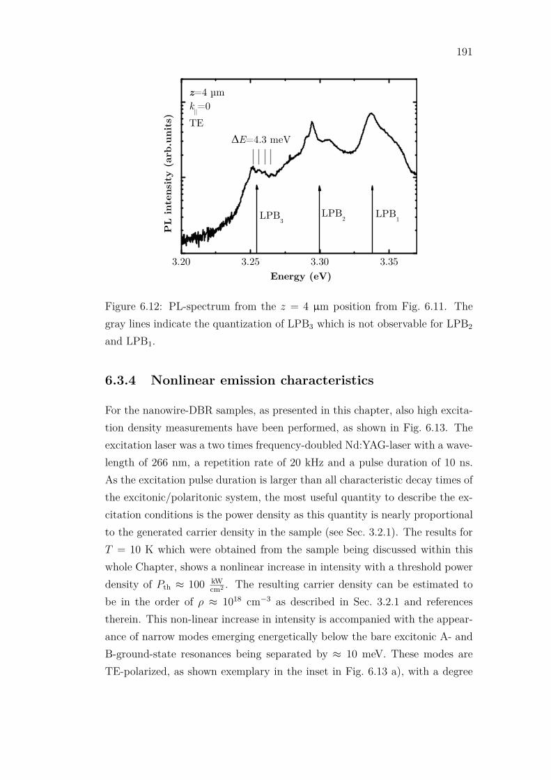
191

3.20 3.25 3.30 3.35

LPB1LPB2

PL

inte

nsit

y (a

rb.u

nits

)

Energy (eV)

LPB3

E=4.3 meV

z=4 µmk||=0TE

Figure 6.12: PL-spectrum from the z = 4 µm position from Fig. 6.11. The

gray lines indicate the quantization of LPB3 which is not observable for LPB2

and LPB1.

6.3.4 Nonlinear emission characteristics

For the nanowire-DBR samples, as presented in this chapter, also high excita-

tion density measurements have been performed, as shown in Fig. 6.13. The

excitation laser was a two times frequency-doubled Nd:YAG-laser with a wave-

length of 266 nm, a repetition rate of 20 kHz and a pulse duration of 10 ns.

As the excitation pulse duration is larger than all characteristic decay times of

the excitonic/polaritonic system, the most useful quantity to describe the ex-

citation conditions is the power density as this quantity is nearly proportional

to the generated carrier density in the sample (see Sec. 3.2.1). The results for

T = 10 K which were obtained from the sample being discussed within this

whole Chapter, shows a nonlinear increase in intensity with a threshold power

density of Pth ≈ 100 kWcm2 . The resulting carrier density can be estimated to

be in the order of ρ ≈ 1018 cm−3 as described in Sec. 3.2.1 and references

therein. This non-linear increase in intensity is accompanied with the appear-

ance of narrow modes emerging energetically below the bare excitonic A- and

B-ground-state resonances being separated by ≈ 10 meV. These modes are

TE-polarized, as shown exemplary in the inset in Fig. 6.13 a), with a degree

192

of polarization of Π = (ITE − ITM)/(ITE + ITM) = 94%. Furthermore, the un-

derlying emission or gain profile shows a clear red shift with increasing pump

power density. The mode spacing together with the red shift of the gain profile

and the estimated threshold carrier density lead to the conclusion that lasing

from WCMs is observed which are fed by an inverted EHP. The observation

that only TE-polarized lasing modes are present, matches with the results ob-

tained from microwire cavities in Chap. 5 and is also explained by the fact

that these modes couple to the electronic system with the intrinsically lower

band gap energy.

At room-temperature (see Fig. 6.13 b) also lasing can be observed, but

here from another nanowire-DBR cavity from the same growth charge as the

cavity which is described before in this chapter. In contrast to the low tem-

perature case, here single mode emission can be observed beyond a power

density threshold of Pth ≈ 2000 kWcm2 . The resulting carrier pair density is then

ρ ≈ 2 × 1019 cm−3 which again yields the recombination in an EHP as the

most probable candidate for the gain mechanism which enables lasing.

For both temperatures, the emission of the LPBs can still be observed be-

yond the lasing threshold. This is mainly caused by the Gaussian beam shape

which was used to excite the samples. Thus, in the center of the excitation

laser spot a higher intensity is present whereas towards the rim of the exci-

tation spot the intensity decreases. Therefore, in the center of the excitation

the Mott density might already been reached whereas at the rim of the exci-

tation spot the strong coupling regime is still present for the LPBs. For the

k‖-resolved measurements as presented in Fig. 6.13, no spatial filtering was

used which results in spectra being integrated over all emitting positions of

the sample.

The reason for not observing exciton-polariton related coherence phenom-

ena below the critical Mott density might be found on the one hand by the

relatively low quality factors and thus relatively large losses. On the other

hand, the high density of WCMs may lead to a fast depletion of the LPB-

ground-states. As the density of WCMs in the FDTD simulations is much

lower as that observed in the real experiments, it seems reasonable that by im-

proving the quality of the DBR-interfaces and reducing thickness fluctuations

of the DBR layers (towards the ideal case as simulated), the WCM-density

193

could be reduced. This together with a higher number of DBR-layer pairs

should enable much higher quality factors and a reduced polariton ground-

state decay which could result in lower threshold laser structures based on

exciton-polariton lasing emission.

Figure 6.13: Excitation power-dependent PL spectra for k‖ = 0 are shown for

T = 10 K and T = 300 K in a) and b), respectively. The inset-graphs in a) and

b) demonstrate the threshold behavior in the input-output characteristics. The

circular inset in a) demonstrates the linear-polarization state of the brightest

mode at 3.336 eV beyond threshold.

6.4 Summary

Within this chapter it was demonstrated that coating a ZnO nanowire with a

radial symmetrical DBR results in a strong lateral optical confinement. This

confinement allowed for the observation of strongly coupled exciton-polaritons

being also stable at room temperature. Strong coupling was thereby proven by

the typical anticrossing behavior in angular-resolved and temperature-dependent

measurements. As a result of the two-dimensional confinement mediated by

a DBR, it was also possible to observe weakly coupled modes which lack in

overlap with the excitons in the nanowire core. The simultaneous appearance

of strong and weak coupling was confirmed by FDTD simulations. Finally,

lasing was demonstrated in our cavity structure up to room-temperature. The

estimated carrier density at threshold and the spectral appearance of the las-

194

ing modes indicate an EHP being the driving gain mechanism for the coherent

emission out of the weakly coupled modes.

Chapter 7

Summary and Outlook

Summary

Within this thesis, planar and wire-like microcavities (MCs) in the strong cou-

pling regime (SCR) have been investigated regarding their dynamical proper-

ties under low and especially under high excitation conditions.

In addition to the experimental work, different approaches for resonance

conditions known from literature were discussed and slightly extended.

A planar MC which was already characterized in detail by H. Franke and C.

Sturm, was investigated regarding the energetic relaxation of exciton-polaritons

in a spatially inhomogenous potential. The sample was known to exhibit SCR

and the formation of coherent sates (BEC) was known to be connected to a

strong blue-shifted potential at the position where the cavity is highly excited.

In the coherent regime beyond the non-linear threshold, the appearance of

discrete relaxation states being nearly equally spaced in energy was theoret-

ically understood as a consequence of balanced in- and out-scattering rates

connected with the relaxation in the potential landscape [WLS10]. The focus

therefore was set on the observation of the emergence of these discrete relax-

ation steps close to the threshold excitation density. In momentum-resolved

measurements, typically no spatial selection is present and the emission from

the central excited area, where the blue-shifted potential is present, might

be masked by the bright emission of the polaritons from the peripheral re-

gion of the potential. Therefore, the micro-photoluminescence (µPL)-setup

was equipped with a pinhole in an intermediate image plane allowing only for

195

196

the observation of the polaritons within the central blue-shifted potential. It

turned out that the discrete relaxation steps are also observable two orders of

magnitude below the actual non-linear threshold, but with an increased spec-

tral spacing. The aforementioned theory which was developed for the coherent

states, could be applied in full analogy to the thermal population of polari-

tons. Therefore, the larger spectral spacing could be explained with the lower

lifetime (given by a larger spectral broadening) of the polariton states and a

bosonic scattering constant could be derived which appears to be independent

of the actual cavity material.

In contrast to planar cavities, in hexagonal microwire (MW) cavities, exciton-

polaritons are confined in two spatial dimension and therefore are only allowed

to propagate freely in the direction of the wire axis. The lateral confinement

is provided by six total internal reflections (TIR) which enables intrinsically

high quality cavities [Wie03]. It was shown by means of the generated charge

carrier density, the spectral position of the underlying gain profile, and by real

and momentum space imaging that with a large excitation spot which exceeds

the lateral dimension of the MW cavity, the low-gain process of polariton-

phonon scattering enables coherent emission from WGM-polaritons below the

critical Mott density at room temperature. In contrast to that, a spatially

narrow excitation spot was used to produce an inverted EHP. The spatially

small pumped region in combination with a large intrinsic coupling constant

ensures that the MW cavities remain in SCR. Thus, the highly excited region

represents only a small perturbation and source for the polariton population.

The obtained results include modal blue shifts which result in polariton states

propagating away from the excitation center. This propagation is accompa-

nied with an measurable expansion of spatial coherence that vastly exceeds the

pumped region by at least one order of magnitude. These observations can be

explained with a model that was initially developed for interacting polariton

BECs [WCC08], but can also be understood under ray-optical considerations

in a cavity with a spatially varying refractive index. The spatially varying

refractive index is thereby given by the locally increased charge carrier den-

sity in the pumped area. In order to reduce the threshold for EHP induced

WGM-polariton lasing, MW cavities were placed in an external DBR-based

Fabry-Pérot (FP) cavity. The external cavity turned out to have a huge im-

197

pact on the WGM quality factors which were increased by at least a factor

of 2. This yielded measurable reduced pump-power threshold densities of up

to a factor of two. In such prepared hybrid MW cavities, hints for negative

Bogoliubov excitations could be found at low temperatures beyond the non-

linear pump density threshold. Thereby, the critical condition as given in

Ref. [Byr+12] regarding blue-shift and mode broadening for the observation

of these excitations is fulfilled and the excitation density threshold for their

appearance is predicted in accordance with the experimental obtained values.

In contrast to the expanding coherent states investigated in detail at room

temperature, the negative excitations show signatures of self-trapping within

the pump spot region.

The last part of the results of this thesis dealt with concentrically DBR-

coated NW-based cavities. There, also one-dimensional polaritons evolve which

are at the border of being zero-dimensional due to the relatively short length

of the NW-cavity. A careful investigation of the angular and spatial polariton

mode dispersion for different temperatures revealed SCR up to room tem-

perature. Furthermore, the coupling of several photonic modes with the A-

and B-excitonic ground-states results in the appearance of middle polariton

branches in PL measurements up to about 100 K. To the knowledge of the

author of this thesis, these branches have never been observed before in PL

experiments in ZnO-based cavities. Their observation was enabled by the high

quality ZnO NWs which exhibit single crystal-like quality. In these NW-based

cavities EHP-induced lasing could also be observed up to room temperature.

Outlook

From the results presented in this thesis, the following tasks remain open for

future investigations.

In general, the observation of upper polariton branches in ZnO based MCs

and connected therewith, the observation of Rabi-oscillations in the time do-

main remain an unsolved problem. This problem could be solved in planar

cavities with the incorporation of quantum well structures instead of bulk-like

cavity layers. For Bragg mirror-coated nanowire-cavities (NW-cavities), this

goal could be achieved with the incorporation of nanometer-thin ZnO NWs

198

with an ultra-high aspect ratio which are already available by now [Shk+17].

Furthermore, the development of longer NW-cavities could provide an impor-

tant building-block for integrated optics as an conduction channel for coherent

states.

For hexagonal-MW cavities, the appearance of phonon-assisted polariton

lasing leaves the question open, if the observed lasing characteristics can also

be explained with a model for doubly stimulated emission as proposed by

H. Krömer [Kro81]. Therefore, it should be searched for signatures of hys-

teresis in power-dependent measurements under cw- or quasi-cw excitation.

As cw-excitation is connected to problematic heat production for elevated ex-

citation densities, it is important to further reduce cavity losses in order to

lower the according pump density threshold. As shown for WGM-polaritons

in hexagonal MW-cavities, their quality factors can be vastly increased, if the

hexagonal wire is incorporated in a planar external DBR-cavity, where leaky

modes from the wire surface are suppressed in only one dimension. Therefore,

it is assumed that a full DBR-coating of all the hexagonal side facets may lead

to further increased quality factors and thus, even more reduced pump-power

threshold values.

The multi-mode polariton structure being present in (thick) MW-cavities

was shown to exhibit parametric scattering effects [Die+15] which could pro-

vide a source for entangled photons [Por+14; Ein+15]. Therefore, quantum

tomography measurements by using a Hanbury-Brown and Twiss setup could

give further insights in the interesting topic of entanglement.

Regarding theory, the realization of propagating coherent polariton states

in SCR as a result of a spatially small electron-hole-plasma (EHP) as source re-

veals some questions. The obtained results imply that many effects, e.g. modal

blue-shift, long-range spatial coherence, particle-particle-interaction, and con-

densation in momentum space can be attributed to exciton-polariton Bose-

Einstein-condensates (BEC) as well as lasers based on an inverted EHP. As

the before-mentioned characteristics are often used to prove the existence of

BEC, it remains an open question to the theory-community to further refine

experimental obtainable criteria for a better differentiability or to provide an

unified theory. Furthermore, already in the 1970s Klingshirn demonstrated

stimulated and directional emission (i.e. condensation in momentum space) as

199

a result of exciton-polariton connected scattering effects in resonator-like ZnO

samples [Kli75]. For such phenomena, as well as exciton-polariton-phonon

scattering as discussed before, the clear distinction (if there is any) to exciton-

polariton-BECs remains diffuse.

Appendix A

Appendix

A.1 Polariton mode splitting

A.1.1 Bulk material mode splitting

In this section the bulk polariton mode splitting is calculated for a material

which has one resonance E0 in the spectral range of interest. High energetic

resonances are introduced by a background dielectric constant ǫb in the DF

ǫ(E).

ǫ(E) = ǫb +f

E20 − E2 + iE2γ

. (A.1)

The polariton equation for a bulk crystal is derived from Maxwell’s equations

to be~

2c2k2

E2= ǫ(E) (A.2)

The solutions (UPB and LPB) of the polariton equation for vanishing damping

of the oscillator (γ = 0) are given by:

E±(k) =1√2ǫb

√f + ~2c2k2 + ǫbE2

0 ±√

(f + ~2c2k2 + ǫbE20)2 − 4~2c2k2ǫbE2

0 .

(A.3)

The mode-splitting Ω is in general defined at the crossing point of bare photon

mode (f = 0) and exciton resonance at k = E0/(~c)√ǫb (see Fig. 2.6):

Ω = E+(k =E0

~c

√ǫb) − E−(k =

E0

~c

√ǫb)) (A.4)

With the substitutions:

a = f + 2ǫbE20 , (A.5)

201

202

b = 4ǫ2bE

40 , (A.6)

c =1√2ǫb

(A.7)

equation (A.4) reads:

Ω = c(√

a+√a2 − b−

√a−

√a2 − b

). (A.8)

By squaring both sides of the equation one gets:

Ω2 = c2(2a− 2√b). (A.9)

The back-substitution leads then to the simple form for the mode splitting:

Ω2 =f

ǫb

. (A.10)

If the broadening γ is taken into account, the UPB and LPB energies at

the crossing point of the uncoupled modes (f=0) are given by:

E±(k =E0

√ǫb

~c) = −i

γ

2+

12

√f

ǫb

− γ2 ± 12

√√√√ f

ǫb

− 2γ2 + 4E20 ∓ i2γ

√f

ǫb

− γ2.

(A.11)

The mode splitting is then given by:

Ω =

√f

ǫb

− γ2 +12

(√a− ib−

√a+ ib

), (A.12)

with a = f/ǫb − 2γ2 + 4E20 and b = 2γ

√fǫb

− γ2. It is easy to see, that

the expression in brackets in eq. (A.12) is purely imaginary for γ < f/ǫb as

only physically valid result. Therefore the mode splitting in the presence of a

broadened resonance is given by:

Ω =

√f

ǫb

− γ2. (A.13)

A.1.2 Cavity mode splitting

The mode dispersion in a cavity is governed by the polariton equation of the

form:~

2c2(k2⊥ + k2

‖)

E2N

= ǫ(E). (A.14)

Here, the wave numbers k⊥ and k‖ represent the absolute value of the quantized

wave vector and of the free wave vector component (in-plane wave number),

203

respectively. For calculating the mode splitting Ω for a vanishing detuning

between the bare cavity mode ground-state (k‖ = 0) and the (excitonic) reso-

nance k⊥ has to be fixed at:

k⊥ =E0

~c

√ǫb. (A.15)

The solutions (UPB and LPB) of the cavity polariton Eq. (2.72) for vanishing

in-plane wave number are:

E±(k⊥) =1√2ǫb

√f + ~2c2k2

⊥ + ǫbE20 ±

√(f + ~2c2k2

⊥ + ǫbE20)2 − 4~2c2k2

⊥ǫbE20 .

(A.16)

As the formal solution is exactly the same as for the bulk polariton case

(see above) the resulting cavity mode splitting:

Ω = E+(k‖ = 0, k⊥ =E0

~c

√ǫb) − E−(k‖ = 0, k⊥ =

E0

~c

√ǫb) (A.17)

is also given by:

Ω2 =f

ǫb

. (A.18)

A.1.3 Cavity mode splitting: Maxwell vs. Hamiltonian

description

In literature, the coupling of a photon mode with a dipole allowed resonance

(exciton, optical phonon etc.) is described with a coupling Hamiltonian of the

form [Sav+95; Pan+99]:

H =

EC − iγC V

V E0 − iγ0

, (A.19)

with the complex bare cavity photon mode energy EC + iγC, the complex

resonance energy E0 +iγ0 and a real coupling constant V . Here, the imaginary

parts describe losses experimentally accessible by mode broadenings (HWHM).

The splitting between the eigen-modes at zero detuning (EC = E0) is given

by:

Ω =√

4V 2 − ((γC − γ0))2. (A.20)

This result claims that the imaginary part of the cavity mode has an influ-

ence on the resonance energies of the coupled system, which compensates the

204

Figure A.1: (a): DBR (with N layer pairs) embedded cavity with refractive

index n(E) and ambient refractive index n0. (b)-(f): Calculated reflectivity

spectra under variation of either the cavity mode broadening γC or the reso-

nance broadening γ0. Calculated reflectivity spectra for N = 0 for a varying

ambient refractive index n0 are shown for a passive and active cavity in (b)

and (c). The dashed lines in (c) indicate the solutions (LPB and UPB) for a

coupled oscillator model with a real cavity mode energy. In (d), the resonance

broadening γ is varied for a constant ambient refractive index (n0 = 1) for

N = 0. In (e), the number of mirror layer pairs N is varied for a constant am-

bient refractive index (n0 = 1) whereas (f) shows the calculated reflectivity for

N = 10 and a varying resonance broadening γ0. The right hand sides of (b)-(f)

show the relative broadenings. The red lines in (b)-(f) show the solutions of

the coupled oscillator model using complex mode energies.

205

influence of the excitonic broadening (γ0). A simple example illustrates that

this is in general not correct. In the following it is shown that the bare cav-

ity mode broadening can be changed without changing the resulting polariton

mode energies or the coupling constant. Let’s consider a material slab with

plan-parallel surfaces without DBRs (N = 0), as sketched in Fig. A.1 a), in an

ambient with refractive n0. The dielectric function of the slab shall be given

by a single resonance E0 with oscillator strength f with vanishing broadening

(γ0 = 0) at first and a background dielectric constant ǫb such that:

ǫ = ǫb +f

E20 − E2

. (A.21)

The reflectivity spectrum1 of such a slab is plotted in Fig. A.1 b) in the vicinity

of the resonance E0 (√ǫb = 10) for varying ambient refractive index n0 and a

vanishing oscillator strength (f = 0). The slab thickness L = ~cπ/(√ǫbE0) is

chosen such that the first bare cavity mode is resonant with E0. By changing

the ambient refractive index, also the broadening γC of the bare cavity mode

(f = 0) is changed as the reflectivity at the slab-ambient interface is changed:

γC = − ~c√ǫbL

ln |rbare| = −E0

πln |rbare|, (A.22)

with rbare = (√ǫb − n0)/(

√ǫb + n0). Figure A.1 c) shows the same as b) but

with a finite oscillator strength of the resonance resulting in a mode splitting

Ω =√f/ǫb = 0.07E0. One can clearly see that the spectral positions of

the reflection dips (reflecting the LPB and the UPB) do not change with

increasing bare cavity mode broadening as predicted by the coupled oscillator

model (A.19) with complex energy of the bare cavity (red lines in Fig. A.1 c)).

In contrast, by ignoring the imaginary part of the bare cavity mode energy,

the coupled oscillator model describes the system correctly (dotted lines in

Fig. A.1 c)). The independence of the coupled mode energies on the cavity

losses results from Ansatz of real-valued energies being used by the software

in order to calculate the reflectivity spectra. This corresponds to the ansatz

of a monochromatic wave.

But also for planar cavities with DBRs mode splittings were calculated

without including cavity losses [VKK96]. While taking into account cavity

1Reflectivity spectra are calculated with the commercial software CompleteEASE from

Woollam.

206

losses in the coupled oscillator model yields predictions for the coupled mode

energies which cannot be measured as dips in the reflectivity, the consider-

ation of electronic resonance losses (excitonic broadening γ0) yields reliable

resonance energies. Figure A.1 d) shows that with increasing resonance broad-

ening, the mode splitting decreases until the splitting vanishes as predicted by

the coupled oscillator model. This happens if the broadening exceeds twice the

coupling strength of the system defining the transition from strong to weak

coupling. Similar statements can be made if a cavity surrounded by DBRs

is considered. Here, the broadening of the cavity mode can be changed (for

constant ambient conditions) if the number of DBR layer pairs is varied. In

Fig. A.1 d) the calculated reflectivity spectra are shown for the same cavity

as before but for increasing N . It is obvious that the bare cavity mode broad-

ening γC decreases with increasing N . An important result is obtained from

the reflectivity spectra of the coupled system: In contrast to the predictions of

the coupled oscillator model, the splitting decreases with increasing layer pair

number N . This is a result of the overlap of the cavity mode x with the elec-

tronic active region which shrinks [Gon+15]. The reduced overlap therefore

leads to a renormalized coupling constant V ′ =√xVbulk which is smaller than

the coupling constant Vbulk of a bulk cavity without DBRs. Finally, the reflec-

tivity of a DBR embedded cavity with N = 10 is plotted for varying resonance

broadening γ0 in Fig. A.1 f). One can see that the mode splitting shrinks with

increasing γ0 until it vanishes as predicted by the coupled oscillator model by

using the renormalized coupling constant V ′.

A.2 Complex mode energies

Real-valued wave number

The implicit formulation of complex cavity resonance energies in the limit of a

real-valued wave number was given by Eq. (2.63) and Eq. (2.64). The explicit

formulation reads:

EN =~c

2L(−mnφ+ 2Nnπ + 2κ ln |r| + Φ)

n2 + κ2(A.23)

and

γN =~c

2L(−2n2 ln |r| − κmnφ+ 2κnNπ + κΦ)

n2 + κ2, (A.24)

207

with

Φ =√n2(mφ− 2Nπ)2 − 4n ln |r|(κmφ− 2Nκπ + n ln |r|). (A.25)

The physical quantities are the same as defined in Sec. 2.3.1.1.

Complex poles in reflectivity

The implicit formulation of the resonance energies of a Fabry-Pérot cavity as

a consequence of searching the complex poles in the reflectivity was given by

Eq. (2.69) and Eq. (2.70). The explicit formulation of the real and imaginary

parts are given by:

EN =~c

dnNπ − φ+ κ

nln |r|

n2 + κ2(A.26)

and

γN =~c

dκNπ − φ− n

κln |r|

n2 + κ2. (A.27)

The physical quantities are the same as defined in Sec. 2.3.1.1.

A.3 Propagation in the non-linear regime:

particle-particle interaction vs. ray-optics

in the presence of a graded refractive in-

dex

This section deals with the similarities of cavity exciton-polariton condensation

and electron-hole plasma lasing. Starting with the particle model for condensed

polaritons it is explained how the real and k-space emission in the presence of

a high density localized polariton reservoir evolves. Then it is shown that the

same emission pattern occurs if the electron-hole density locally approaches

the Mott density. This is explained as a result of a local change in the DF

of the cavity material. Finally, properties are identified allowing to distinct

between these two processes.

In literature dealing with polariton Bose-Einstein condensation, often the

condensation occurs on a ring in k-space whose energy is blue-shifted by ∆E

from the LPB ground-state [Hou+00; Ric+05; Fra+12], as shown in Fig. A.2,

usually when the condensate is created in a small spatial area. Wouters et

208

Epot

x

Ea) b) c)

Figure A.2: Polariton dynamic above the nonlinear threshold: (a) two di-

mensional angular distribution and (b) emission energy vs. angle, taken

from [Ric+05]. (c) sketch of the repulsive polariton-polariton interaction re-

sulting in an acceleration out the region with the highest polariton density

under conservation of total energy.

al. [WCC08] developed a description of this phenomenon in the frame of solv-

ing the Gross-Pitaevskii equation (GPE). They argue that the blue-shift at the

center of the excitation area is created by the repulsive interaction between

condensed polaritons among each other, uncondensed polaritons and with a

not specifically defined potential that is created by the pump laser. An im-

portant point is that the resulting spatially varying potential should act on

the entire polariton system and thus, on the LPB and the UPB in the same

way. Furthermore, Wouters et al. explain that the condensation sets in in

the center of the excitation area where the particle density is highest at zero

in-plane wave vector. As the GPE represents energy conservation, the full

potential energy ∆E = Epot of the condensed polaritons is transferred into

kinetic energy,

Epot = Ekin, (A.28)

when the condensate is accelerated out of the central excitation area due to

the potential gradient. The kinetic energy Ekin is given by:

Ekin =~

2k2‖

2m, (A.29)

with m being the polariton mass. From this consideration it is clear that the

maximum accessible wave number value k‖max is determined by the LPB disper-

sion of the uncondensed polaritons, which is given by the r.h.s. of Eq. (A.29) in

209

the parabolic dispersion approximation. The maximum reachable wave num-

ber value is therefore:

k‖max =√

2m∆E/~2. (A.30)

A second possible physical model which reproduces the same emission pat-

tern in real and k-space, as shown in Fig. A.2, is the following: It is well known

that with increasing carrier density, the excitonic transition energies stays more

or less constant2 whereas the oscillator strength f decreases slowly and drops

rapidly by approaching the Mott density (see [Zim+78] and references therein).

The effect of a reduced oscillator strength leads directly to a blue-shifted LPB,

whereas the UPB is red-shifted in contrast to the particle picture discussed

above. This follows from the polariton equation for finite sized cavities of the

optical length n(λ)L, where the resonant wavelengths (polariton branches) are

given by:

Nλ = n(λ)L. (A.31)

In the energy notation this reads:

E =hcN

n(E)L. (A.32)

The r.h.s. and l.h.s. of Eq. (A.32) are plotted in Fig. A.3 for three different

values of the oscillator strength. If we assume that the energy shift ∆E of

the LPB in Eq. (A.29) is a consequence of the reduced oscillator strength

resulting in a local change of the refractive index ∆n, then, for small blue-

shifts (∆E << E0), one can define from Eq. (A.31):

∆E ≃ − hcL

λ20N

∆n, (A.33)

with λ0 being the resonance wavelength. The polariton mass m in a pure bulk

cavity can be derived by the Taylor expansion of E(k‖) = ~c√k2

0 + (k‖/n)2 ∼E0 + ~

2k2‖/(2m) to be

m ≃ hNn

Lc. (A.34)

2The constant transition energy is a result of two counter acting processes. On the

one hand, the increasing particle density leads to a screening of the Coulomb potential of

the electron-hole pair system which results in a reduced binding energy and therefore in a

blue-shifted resonance energy. On the other hand, the band gap shrinks due to band gap

renormalization [Zim+78; Gru06].

210

Ecav

UP B2

LP B2

UP B1

hc/ (nL) f= 0.1E0

hc/ (nL) f= 0.05E0

hc/ (nL) f= 0.0

E

E (arb. unit s)

LP B1

γ= 0

Figure A.3: Plotted values for the r.h.s and l.h.s. of Eq. A.32 for vanish-

ing damping and different oscillator strengths. The crossing between E and

hc/(nL) gives the polariton branches of the system.

Inserting m and ∆E in Eq. (A.30) connects the maximum k-value with the

refractive index change for the LPB:

k‖max ≃ 2πλ0

√−2n∆n. (A.35)

It is well known from ray optics that in the presence of a refractive index

gradient the light’s ray path is bent into the direction of the higher refractive

index [LL80]. This means that within a resonator the in-plane wave vector

increases in the direction of higher refractive index. This is sketched in Fig. A.4

where a slab with a spatially varying refractive index n(x) is sketched. The

invariant of the system under propagation in the slab is n0 sin θ0. This leads

to:

n0 sin θ0 = n(x) sin θ(x), (A.36)

with n0 = n + ∆n and θ0 being the initial refractive index and angle at the

x-position of the slab with highest particle density (lowest refractive index for

the LPB). The refractive index in the unexcited region is n. If the photon

leaves the cavity at the position x it will have the angle θa with respect to the

cavity normal which is given by:

θa = sin−1(√

n(x)2 − n20 sin2 θ

). (A.37)

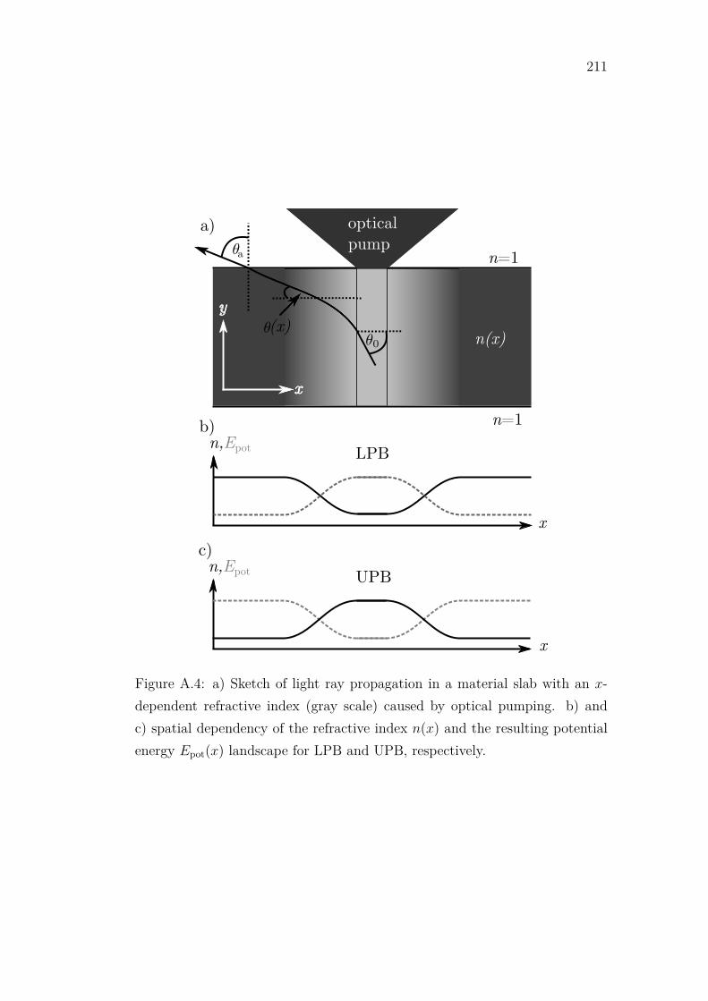
211

Figure A.4: a) Sketch of light ray propagation in a material slab with an x-

dependent refractive index (gray scale) caused by optical pumping. b) and

c) spatial dependency of the refractive index n(x) and the resulting potential

energy Epot(x) landscape for LPB and UPB, respectively.

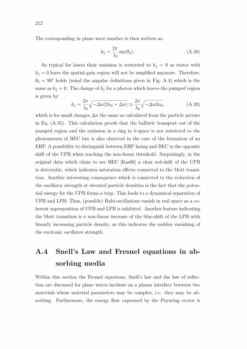
212

The corresponding in plane wave number is then written as:

k‖ =2πλ0

sin(θa). (A.38)

As typical for lasers their emission is restricted to k‖ = 0 as states with

k‖ = 0 leave the spatial gain region will not be amplified anymore. Therefore,

θ0 = 90 holds (mind the angular definitions given in Fig. A.4) which is the

same as k‖ = 0. The change of k‖ for a photon which leaves the pumped region

is given by:

k‖ =2πλ0

√−∆n(2n0 + ∆n) ≃ 2π

λ0

√−∆n2n0, (A.39)

which is for small changes ∆n the same as calculated from the particle picture

in Eq. (A.35). This calculation proofs that the ballistic transport out of the

pumped region and the emission in a ring in k-space is not restricted to the

phenomenon of BEC but is also observed in the case of the formation of an

EHP. A possibility to distinguish between EHP lasing and BEC is the opposite

shift of the UPB when reaching the non-linear threshold. Surprisingly, in the

original data which claim to see BEC [Kas06] a clear red-shift of the UPB

is detectable, which indicates saturation effects connected to the Mott transi-

tion. Another interesting consequence which is connected to the reduction of

the oscillator strength at elevated particle densities is the fact that the poten-

tial energy for the UPB forms a trap. This leads to a dynamical separation of

UPB and LPB. Thus, (possible) Rabi-oscillations vanish in real space as a co-

herent superposition of UPB and LPB is inhibited. Another feature indicating

the Mott transition is a non-linear increase of the blue-shift of the LPB with

linearly increasing particle density, as this indicates the sudden vanishing of

the excitonic oscillator strength.

A.4 Snell’s Law and Fresnel equations in ab-

sorbing media

Within this section the Fresnel equations, Snell’s law and the law of reflec-

tion are discussed for plane waves incident on a planar interface between two

materials whose material parameters may be complex, i.e. they may be ab-

sorbing. Furthermore, the energy flow expressed by the Poynting vector is

213

investigated. The first part deals with the inhomogenous plane wave (IPW)

as a general solution of Maxwell’s equations and the dispersion relation which

has to be fulfilled by the IPW. The second part discusses two special cases. On

the one hand the reflection and transmission properties on an absorbing/non-

absorbing interface are discussed for probing with a homogenous plane wave

(HPW) being incident from a non-absorbing material. This situation leads

to a purely real in-plane wave vector at plan-parallel interfaces and is impor-

tant for reflection or ellipsometry measurements. The second case which is

discussed describes HPW in absorbing media and their reflection and trans-

mission properties at a planar interface to vacuum. This case accounts for

HPW which are created in an absorbing medium (e.g. in photoluminescence)

or for guided modes. This is of special interest as it is important to describe

whispering gallery modes in resonators of absorbing material. Independent of

the case which is described, the same set of equations can be used for a com-

prehensive description of the problem. The following considerations are only

valid for isotropic and nonmagnetic materials.

A.4.1 Inhomogenous plane waves

A.4.1.1 Definitions and dispersion relation

A solution of Maxwell’s equations in an unbound medium is given by [Jac82]:

~E(~r, t) = ~E0ei(~k·~r−ωt), (A.40)

with

~k = k0n~n. (A.41)

Here ~E0 and ~n describe the, in general complex, temporal and spatial indepen-

dent electric field and direction vectors, respectively. The angular frequency

is introduced by the real valued quantity ω. The vector ~n has to obey

~n · ~n = 1 (A.42)

to fulfill the dispersion relation

~k · ~k = (nω/c)2, (A.43)

214

and therefore Maxwell’s equations [Jac82; DAP94a]. After [Jac82; DAP94a] ~n

can be written as:

~n = ~n‖ cosh β + i ~n⊥ sinh β, (A.44)

with ~n‖ and ~n⊥ being orthogonal real unit vectors as sketched in Fig. A.5.

ii x

z

r

tt

Figure A.5: Angular definitions, coordinate system and directions of vector

components as described in the main body of the text.

The real valued β is called inhomogeneity factor and can be chosen positive

as ~n remains unchanged under reversion of the signs of ~n⊥ and β. An inho-

mogeneity (β > 0) is always connected to an interface or boundary conditions

at infinity [DAP94a]. The isotropic medium is characterized by the complex

refractive index n = n + iκ. Planes of constant phase are characterized by

Re[~k] · ~r = 0 and planes of constant amplitude by Re[~k] · ~r = 0. According to

reference [Smi97] an inhomogenous plane wave (IPW) is present if these two

planes do not coincide. A well known example for an inhomogenous wave is

the evanescent wave in the case of total internal reflection (TIR) at an interface

between two non-absorbing dielectric media. There the amplitude decreases in

the direction perpendicular to the interface whereas the phase front propagates

along the boundary.

A.4.1.2 Snell’s Law and Fresnel equations

The case of an arbitrary IPW hitting an interface between two (absorbing)

dielectrica has been fully treated in reference [DAP94a]. Here the simpler case

of an incident IPW with the inhomogeneity located in the plane of incidence

is studied. If the normal unit vector of the interface is given by ~s the general

215

formulation of the conservation of the in-plane wave vectors

~s× ~ki = ~s× ~kr = ~s× ~kt, (A.45)

with the subscripts j = t, r, i describing the incident, reflected and transmitted

wave yields:

θi = θr, (A.46)

ni sin θi = nt sin θt, (A.47)

and

θj = θj − iβj, (A.48)

with θi,r,t being a complex quantity in general. For the conditions described

above the Fresnel equations for reflection (rj) and transmission (tj) have the

usual form for s- and p-polarization [DAP94a; Byr16]:

rs =ni cos θi − nt cos θt

ni cos θi + nt cos θt

ts =2ni cos θi

ni cos θi + nt cos θt

(A.49)

rp =nt cos θi − ni cos θt

nt cos θi + ni cos θt

tp =2ni cos θi

ti cos θi + it cos θt

. (A.50)

The convention for the sign of rp which has been chosen here, states that for

normal incidence a phase difference of π between s- and p- is present. It is

the same convention as used in reference [Cze+10] for their plane wave model

(formula (2) of [Cze+10]) in order to obtain the WGM resonance energies.

Reference [Byr16] includes a helpful discussion about the sign convention con-

cluding that non of both possibilities is more right or wrong.

Special attention has to be taken into account by implementing the compo-

nents ni,t cos θt which are derived by Snell’s law to be:

ni,t cos θt = ± ni,t

nt

√n2

t − (ni sin θi)2 = p+ qi. (A.51)

The sign convention here is not arbitrary. For the standard case discussed here,

with positive refractive indices (forward traveling modes) and positive extinc-

tion coefficients (absorption) both, p = Re[ni,t cos θt] and q = Im[ni,t cos θt]

have to be positive in order to avoid unphysical results. With Re[ni,t cos θt] < 0

backward traveling waves introduce reflectivities larger one and Im[ni,t cos θt] <

0 results in exponentially increasing amplitudes.

216

As an example for angular dependent complex reflection coefficients, in

Fig. A.6 the reflectivity |r|2 and the phase Arg(r) are plotted for a HPW

incident on an interface from an optically thicker to a thinner medium for the

case with and without absorption. In the case of non-vanishing absorption,

total internal reflection is attenuated.

0 20 40 60 800.0

0.2

0.4

0.6

0.8

1.0 p; s; p; s;

|r|2

i

Figure A.6: Calculated angular dependent reflectivity for the reflection of a

HPW incident on the interface to an optical thinner medium (here: vacuum)

from a medium without (solid lines) or with (dashed lines) extinction κ for s

and p polarization.

A.4.1.3 Energy flow and Poynting vector

The (complex) Poynting vector describing the direction and magnitude of the

energy flow of a wave and is defined by

~S(~r, t) = ~E(~r, t) × ~H(~r, t), (A.52)

where ~H(~r, t) describes the (complex) magnetic field, which is induced by the

varying electric field (and vice versa):

~k × ~E(~r, t) = µ0ω ~H(~r, t), (A.53)

217

with µ0 being the magnetic permeability. For the case of an IPW ~k(~r, t)×~S(~r, t)

does not vanish and is in general a function of time [DAP94a; DAP94b; CL11],

reflecting the time dependent direction(!) and magnitude of the Poynting

vector [CL11]. This directly implies a decaying IPW even in a non-absorbing

medium. Examples are given below.

A.4.2 Important examples

In this section two special examples for the appearance if IPWs are demon-

strated which are directly connected to interfaces including lossy media.

A.4.2.1 Reflection and ellipsometry measurements: real in-plane

wave vectors

Reflection or ellipsometry measurements on planar layer stacks are typically

performed in a non-absorbing ambient (air or vacuum) with a HPW (β = 0)

as incident wave. This leads to the fact that the projection of the wave vector

on the interface, k0n sin θ, is purely real. If the probed medium is absorbing

(ni = ni + iκi, κi > 0) the direction vector ~ni has to be complex in order to

achieve the conservation of the in-plane wave vectors resulting in an IPW in

the absorbing medium. This requirements yield an angular dependent value

for β given by:

β = | tanh−1[−κi

ni

tan θi

]|. (A.54)

For this, Eq. (A.44) was used including the normal vectors ~n‖ = (sin θi, cos θi)T

and ~n⊥ = (− cos θi, sin θi)T with θi being the angle describing the real part of

the direction vector ~n. Now we consider this IPW being incident at an interface

to vacuum (nt = 1) at infinite distance to the first interface (to exclude multiple

reflections). For simplicity this second interface should be parallel to the first

interface. The reflectivity and phases are plotted in Fig. A.7 and the real part

of the electric field in the vicinity of a boundary is plotted in Fig. A.8 for

oblique incidence. The reflectivity shows, similar to the non-absorbing case, a

Brewster angle (minimum in reflectivity for p-pol.) and a critical angle for TIR.

Both are shifted towards higher angles. It has to be mentioned that within the

experimental scenario described here, with two plan-parallel interfaces, angles

larger than the critical angle for TIR are not reachable. As a result of the

218

conservation of the in-plane wave vectors and of the final medium being the

same as the initial, the transmitted wave in this example is a HPW again.

0 20 40 60 800.0

0.2

0.4

0.6

0.8

1.0

0 20 40 60 80-3

-2

-1

0

p; s; p; s;

|r|2

i

b)a) p; s; p; s;

Arg

[r]

i

Figure A.7: Angular dependent reflection of a plane wave at an interface to

vacuum for real in-plane wave vector components: reflectivity (a) and phase

(b) for ni = 2 and κi = 0 (lines) and κi = 0.1 (dashed) for s- and p-polarization.

If absorption is present, the incident wave is an IPW.

As mentioned before, the direction and magnitude of the Poynting vector

for an IPW is time dependent. For the case described here, with an IPW in

the absorbing layer, this is graphically shown on the left side in Fig. A.9 for a

HPW incident under 20 from vacuum. It is clearly visible that with increasing

extinction the angular broadening also increases connected with a shift of the

angular center of the distribution.

A.4.2.2 Photoluminescence from an active layer: complex in-plane

wave vectors

In photoluminescence experiments (PL) a high photon energy laser beam typ-

ically excites carriers close to the surface of an absorbing medium. If these

carriers recombine they can emit photons inside the absorbing medium. As

the resulting electromagnetic wave was not entering the absorbing material

219

Figure A.8: Left: sketch of the involved wave vectors for an IPW incident

from an absorbing layer on the interface to vacuum (real in-plane wave vector

components). Right: real part of the electric field of a s-polarized IPW incident

on an interface to vacuum under 20 (real part of the direction vector) for a

real in-plane wave vector. The medium in which the incident wave travels is

characterized by n = 2 + 0.1i. The reflected wave is also included resulting in

the electric field being continuous across the boundary.

by crossing an interface, the surface normals of planes of constant phase and

amplitude are parallel. If the excited area is sufficiently large the assumption

of having HPW in the absorbing media is valid (Huygens’ principle). PL en-

ables therefore also the occupation of waveguide modes whose internal angle

is larger than the critical angle for TIR, which is not possible with standard

reflectivity or ellipsometry measurements.

Again, we are interested in the reflection and transmission properties, in

this with an HPW incident on the interface between an absorbing medium

and vacuum. The results are plotted in Fig. A.11. It is obvious that in this

case the phases and amplitudes of the reflection coefficients differ from the

case described before, where the in-plane component of the wave vector was

purely real. Furthermore, no defined angle for TIR is present anymore. As

a result of the conservation of the in-plane wave vector component also the

transmitted wave vector is complex resulting in a IPW in vacuum for oblique

incidence. This means the IPW in vacuum decays with distance from the

interface with the direction of the real and imaginary parts of the wave vector

being perpendicular as sketched in Fig. A.11.

220

0 200.0

0.5

1.0

30 35 40 45 50 550.0

0.5

1.0 1 0.1 0.01 0.001 0.0001

Nor

m(|

Re[S]

|) (

arb.

uni

ts)

Angle of Re[S] (degree)

t

b)i 1

0.1 0.01 0.001 0.0001

Nor

m(|

Re[S]

|) (

arb.

uni

ts)

Angle of Re[S] (degree)

a)

Figure A.9: Poynting vector and energy flow for IPWs. a): Angular distri-

bution of the energy flow for an IPW in an absorbing medium (nt = 2) in

dependence of the extinction coefficient κt. Here the IPW was created from an

HPW incident from vacuum under θi = 20. b): Angular distribution of the

energy flow for an IPW in vacuum in dependence of the extinction coefficient

κi of the initial medium. In the initial medium the wave is supposed to be an

HPW incident on the interface to vacuum under θi = 20.

221

The decay of the IPW in vacuum is again easily understood if the Poynting

vector is considered (see right side of Fig. A.9). In dependence on the extinc-

tion coefficient in the initial medium, the angular broadening of the Poynting

vector’s direction in vacuum increases resulting in a divergent wave in vacuum.

0 20 40 60 800.0

0.2

0.4

0.6

0.8

1.0

0 20 40 60 80

-3.0

-2.5

-2.0

-1.5

-1.0

-0.5

0.0b)

p; s; p; s;

|r|2

i

a) p; s; p; s;

Arg

[r]

i

Figure A.10: Angular dependent reflection of a HPW at an interface to vac-

uum: reflectivity (a) and phase (b) for ni = 2 and κi = 0 (lines) and κi = 0.1

(dashed) for s- and p-polarization. If absorption is present, the transmitted

wave is an IPW.

A.5 Angular- and spatial-resolved imaging

For the investigation of systems where light is confined in one or more dimen-

sions angular-resolved PL or reflectivity spectra give access to sample proper-

ties as a function of in-plane momemtum. This is done by using a converging

lens or lens system (objective). This optical elements are able to Fourier-

transform (FT) the electrical field distribution Ereal(x, y) from the real space

into the momentum space distribution EFourier(kx, ky) [Hec05]:

Ereal(x, y)lens=F T︷ ︸︸ ︷⇐⇒ EFourier(kx, ky). (A.55)

222

z k0)

x k0)

❬ E

/E0❪

x

z

Figure A.11: Left: sketch of the involved wave vectors for an HPW incident

from an absorbing layer on the interface to vacuum. Right: real part of the

electric field of a s-polarized HPW incident on an interface to vacuum under

20 (real part of the direction vector). The medium in which the incident

wave travels is characterized by n = 2 + 0.1i. The reflected wave is also

included resulting in the electric field being continuous across the boundary.

The transmitted wave is an IPW.

This means, that the lens (objective) images parallel light rays, which are com-

ing from the object-plane as a point image in the Fourier plane, as shown in

Fig. A.12. The Fourier plane corresponds to the back-focal plane of the lens

(objective). In other words, the lens images the far-field distribution of the

object plane onto its back-focal plane at the distance f ′. The term far-field

refers to parallel rays, which intersect at an infinite distance. Introducing the

converging lens, shifts that intersection point from infinity to a finite distance

f ′. The in-plane momentum vector (px, py) is the projection of the wave vec-

tor on the plane perpendicular to the optical axis given by the lens. It is

proportional to the in-plane wave vector (kx, ky)

(px, py) = ~(kx, ky) =2πλ

(sin θ, sin ρ), (A.56)

with k being the wave number and (θ, ρ) giving the angle between the prop-

agation direction and the optical axis. The mathematical formulation of the

FT introduced by the lens is given by:

EFourier(kx, ky) =∫∫ ∞

−∞Ereal(x, y)e−i(xkx+yky)dxdy. (A.57)

223

Figure A.12: Sketch of a converging lens focusing parallel rays on one point in

its back-focal or Fourier plane.

The connection between a point in the Fourier-plane with real space coordi-

nates (Kx, Ky) and the propagation direction (θ, ρ) in front of the lens can

easily be obtained by:

(Kx, Ky) = f ′(tan θ, tan ρ), (A.58)

which is sketched in Fig. A.12. The Fourier plane is bounded by the maximum

in-plane wave number kmax which is given by the numerical aperture (NA) of

the lens or objective. The NA is a measure of the maximal detectable angle

θmax of the lens (objective) with respect to the optical axis:

NA = n sin θmax = nλkmax

2π. (A.59)

A second converging lens, following the first one, images an inverted image

of the object plane in the Fourier plane of the second lens (see Fig. A.14). The

second lens performs a second FT. Here, the NA of the first lens determines the

maximum available in-plane wave numbers, which represent the boundaries of

the interval over which is integrated in this Fourier synthesis. This leads to

the fact, that a point source in the object plane is imaged as a Airy disk in

the image plane:

Eimage(Y ) =1

2π

∫ kmax

−kmax

E0e−ikyY dkY . =

E0

Y πsin (Y kmax) (A.60)

The general n-dimensional Fourier synthesis can be written as [BW05]:

Eimage( ~X) =1

(2π)n

∫ ∞

−∞EF ourier(~k) exp−i~k ~X dXn (A.61)

224

y

x

Ky

Kx

Figure A.13: Sketch for the visualization of the connections between the emis-

sion directions (θ, ρ) out of the object plane, their corresponding in-plane wave

vector components (kx, ky) and their projection in the Fourier plane P(Kx, Ky).

A converging lens has not been drawn for clarity.

225

The separability of two of such Airy disks gives the resolution of microscopes

and lenses and is proportional their NA. As the maximum in-plane wave

numbers are inverse proportional to the wavelength of the light (kmax =2πλ

sin θmax), the resolution is also inverse proportional to the wavelength of

light. For the minimal distance, at which two of such Airy disks are still sepa-

rable, the Rayleigh criterion holds. It states, that two Airy disks are separable

until the maximum of one of them is located at the first minimum of the second

one:

∆y = 0.61λ

NA. (A.62)

Figure A.14: Sketch of the image formation of a point source via two converging

lenses. On the right side the intensity distribution is drawn exemplary for a

finite numerical aperture of the lens system.

Bibliography

[AC79] G. P. Agrawal and H. J. Carmichael: Optical bistability through

nonlinear dispersion and absorption, Phys. Rev. A 19 (1979),

2074–2086.

[AD93] G. P. Agrawal and N. K. Dutta: Semiconductor lasers. Van Nos-

trand Reinhold, New York, 1993.

[Amo+09] A. Amo et al.: Superfluidity of polaritons in semiconductor mi-

crocavities, Nat. Phys. 5 (2009), 805–810.

[And94] L. C. Andreani: Exciton-polaritons in superlattices, Phys. Lett. A

192 (1994), 99–109.

[Bal+17] D. Ballarini et al.: Macroscopic two-dlimensional polariton con-

densates, Phys. Rev. Lett. 118 (2017), 215301.

[Bay03] M. Bayer: Control of light-matter interaction in microresonators,

Physica E 17 (2003), 393–397.

[BKC16] S. J. Byrnes, M. Khorasaninejad, and F. Capasso: High-quality-

factor planar optical cavities with laterally stopped, slowed, or re-

versed light, Opt. Express 24 (2016), 18399.

[Blo+97] J. Bloch et al.: Strong-coupling regime in pillar semiconductor

microcavities, Superlattices and Microstructures 22 (1997), 371–

374.

[Bog47] N. N. Bogoliubov: On the Theory of Superfluidity, J. Phys. USSR

11 (1947), 23–32.

[Bra76] A. I. Braunstein: Calculation of electrical field and absorption in

thin film structures, Thin Solid Films 37 (1976), 181.

227

228 BIBLIOGRAPHY

[Bro65] L. de Broglie: The wave nature of the electron In: Nobel Lectures,

Physics 1922-1941. Elsevier Publishing Company, 1965.

[BSS08] C. Bundesmann, R. Schmidt-Grund, and M. Schubert: “Optical

Properties of ZnO and Related Compounds”. English. In: Trans-

parent Conductive Zinc Oxide. Ed. by K. Ellmer, A. Klein, and

B. Rech. Vol. 104. Springer Series in Materials Science. Springer

Berlin Heidelberg, 2008, pp. 79–124.

[BW05] M. Born and E. Wolf: Principles of Optics, 7th (expanded) edition.

The Press Syndicate of the University of Cambridge, 2005.

[Byr+12] T. Byrnes et al.: Negative Bogoliubov dispersion in exciton-polariton

condensates, Phys. Rev. B 85 (2012), 075130.

[Byr16] S. J. Byrnes: Multilayer optical calculations, arxiv arXiv:1603.02720v2

[physics.comp-ph] (2016).

[Cao+09] B. Q. Cao et al.: Homogeneous core/shell ZnO/ZnMgO quantum

well heterostructures on vertical ZnO nanowires, Nanotechnology

20 (2009), 305701.

[Cas75] L. W. Casperson: Threshold characteristics of multimode laser

oscillators, J. Appl. Phys. 46 (1975), 5194–5201.

[Chr+07] S. Christopoulos et al.: Room-Temperature Polariton Lasing in

Semiconductor Microcavities, Phys. Rev. Lett. 98 (2007), 126405.

[Chr94] G. H. D. Chrisey: Pulsed Laser Deposition of Thin Films. Wiley,

1994.

[CL11] J. Chen and H. Lu: Generalized laws of reflection and refraction

from real valued boundary conditions, Opt. Commun. 284 (2011),

3802–3807.

[Cze+08] C. Czekalla et al.: Whispering gallery mode lasing in zinc oxide

microwires, Appl. Phys. Lett. 92, 241102 (2008), 241102.

[Cze+10] C. Czekalla et al.: Whispering gallery modes in zinc oxide micro-

and nanowires, Phys. Status Solidi B 247 (2010), 1282–1293.

[Cze09] C. Czekalla: “Ortsaufgelöste Lumineszenz von Zinkoxid-Mikronadeln”.

PhD thesis. Universität Leipzig, 2009.

BIBLIOGRAPHY 229

[Dai+09a] J. Dai et al.: Combined whispering gallery mode laser from hexag-

onal ZnO microcavities, Appl. Phys. Lett. 95, 191117 (2009),

191117.

[Dai+09b] J. Dai et al.: Whispering gallery-mode lasing in ZnO microrods at

room temperature, Appl. Phys. Lett. 95, 241110 (2009), 241110.

[Dai+10] J. Dai et al.: Exciton and electron-hole plasma lasing in ZnO do-

decagonal whispering-gallery-mode microcavities at room temper-

ature, Appl. Phys. Lett. 97, 011101 (2010), 011101.

[Dai+11a] J. Dai et al.: Exciton-polariton microphotoluminescence and las-

ing from ZnO whispering-gallery mode microcavities, Appl. Phys.

Lett. 98, 161110 (2011), 161110.

[Dai+11b] J. Dai et al.: Response to Comment on Exciton-polariton mi-

crophotoluminescence and lasing from ZnO whispering-gallery mode

microcavities [Appl. Phys. Lett. 99, 136101 (2011)] , Appl. Phys.

Lett. 99, 136102 (2011), 136102.

[Dai+11c] J. Dai et al.: Three-photon absorption induced whispering gallery

mode lasing in ZnO twin-rods microstructure, Opt. Mater. 33

(2011), 288–291.

[DAP94a] M. A. Dupertuis, B. Acklin, and M. Proctor: Generalization of

complex Snell–Descartes and Fresnel laws, J. Opt. Soc. Am. A

11 (1994), 1159–1166.

[DAP94b] M. A. Dupertuis, B. Acklin, and M. Proctor: Generalized energy

balance and reciprocity relations for thin-film optics, J. Opt. Soc.

Am. A 11 (1994), 1167–1174.

[Dav+95] K. B. Davis et al.: Bose-Einstein Condensation in a Gas of Sodium

Atoms, Phys. Rev. Lett. 75 (1995), 3969–3973.

[DG11] C. P. Dietrich and M. Grundmann: Comment on Exciton-polariton

microphotoluminescence and lasing from ZnO whispering-gallery

mode microcavities [Appl. Phys. Lett. 98, 161110 (2011)] , Appl.

Phys. Lett. 99, 136101 (2011), 136101.

[DHY10] H. Deng, H. Haug, and Y. Yamamoto: Exciton-polariton Bose-

Einstein condensation, Rev. Mod. Phys. 82 (2010), 1489–1537.

230 BIBLIOGRAPHY

[Die+11] C. P. Dietrich et al.: One- and two-dimensional cavity modes in

ZnO microwires, New J. Phys. 13 (2011), 103021.

[Die+15] C. P. Dietrich et al.: Parametric relaxation in whispering gallery

mode exciton-polariton condensates, Phys. Rev. B 91 (2015), 041202.

[Die+16] C. P. Dietrich et al.: An exciton-polariton laser based on biologi-

cally produced fluorescent protein, Science Advances 2 (2016).

[Die12] C. P. Dietrich: “Cavity effects in polygonal resonators”. PhD the-

sis. Universität Leipzig, 2012.

[Din+12] M. Ding et al.: The ultraviolet laser from individual ZnO mi-

crowire with quadrate cross section, Opt. Express 20 (2012), 13657–

13662.

[DXS11] J. Dai, C. X. Xu, and X. W. Sun: ZnO-Microrod/p-GaN Het-

erostructured Whispering-Gallery-Mode Microlaser Diodes, Adv.

Mater. 23 (2011), 4115–4119.

[Ein+15] L. Einkemmer et al.: Polarization entanglement generation in mi-

crocavity polariton devices, Phys. Status Solidi B 252 (2015),

1749–1756.

[Ein05] A. Einstein: Ist die Trägheit eines Körpers von seinem Energiein-

halt abhängig?, Ann. Phys. 18 (1905), 639–641.

[Ein25] A. Einstein: Quantentheorie des idealen Gases- Zweite Abhand-

lung, Sitzungsberichte der preussischen Akademie der Wissenschaften

1 (1925), 3–10.

[EKR08] K. Ellmer, A. Klein, and B. Rech, eds.: Transparent conductive

zinc oxide. Springer, 2008.

[Fal+08] J. Fallert et al.: Lasing dynamics in single ZnO nanorods, Opt.

Express 16 (2008), 1125–1131.

[Fau+08] S. Faure et al.: Comparison of strong coupling regimes in bulk

GaAs, GaN, and ZnO semiconductor microcavities, Phys. Rev. B

78 (2008), 235323.

[Fau+09] S. Faure et al.: Relaxation and emission of Bragg-mode and cavity-

mode polaritons in a ZnO microcavity at room temperature, Ap-

plied Physics Letters 95 (2009), 121102.

BIBLIOGRAPHY 231

[Fra+12] H. Franke et al.: Ballistic propagation of exciton-polariton con-

densates in a ZnO-based microcavity, New J. Phys. 14 (2012),

013037.

[Fra12] H. Franke: “PLD-grown ZnO-based Microcavities for Bose-Einstein

Condensation of Exciton-Polaritons”. PhD thesis. Universität Leipzig,

2012.

[Fre31] J. Frenkel: On the transformation of light into heat in solids, Phys.

Rev. 37 (1931), 17.

[Fuj07] H. Fujiwara: Spectroscopic ellipsometry: Principles and applica-

tions. Wiley, 2007.

[Gal+12] M. Galbiati et al.: Polariton Condensation in Photonic Molecules,

Phys. Rev. Lett. 108 (2012), 126403.