Progressive Taxation and Redistribution Democracy and Inequality in the Americas Notre Dame, April 8 2019 Pablo Beramendi Duke University Matthew Dimick SUNY Buffalo Law School Daniel Stegmueller Duke University

Welcome message from author
This document is posted to help you gain knowledge. Please leave a comment to let me know what you think about it! Share it to your friends and learn new things together.
Transcript

Progressive Taxation and Redistribution
Democracy and Inequality in the AmericasNotre Dame, April 8 2019
Pablo Beramendi
Duke University
Matthew Dimick
SUNY Buffalo Law School
Daniel Stegmueller
Duke University

Progressivity and Redistribution [1]
Motivation
É As Inequality and Taxation return to public debate, two “venerable questions” on theirway back:
1. Is “taxing the rich” the most effective way to pursue redistribution curb down inequal-ity? Do arguments on wealth (Piketty, Zucman, Scheve and Stasavage) translate wellinto income?
2. Under what conditions are sustainable coalitions pro R feasible?
É Need to revisit the connection between Redistribution and Tax Progressivity.
É Theoretically, the field is a bit of a conceptual mess:
1. Inverse relationship between redistribution and progressivity of tax structures (Kato2003, Ganghof 2006, Lindert 2004, B& R 2007, Prasad and Deng 2009, Martin 2015,Piketty et al. 2014)
2. Paradox of Redistribution (Korpi and Palme 1999, B & R 2016)
3. All the action regarding redistribution is on the spending side, taxes being irrelevant(e.g., Kenworhty)
4. And then there is common sense...
É Empirically, a festival of partial approaches overlooking two issues:
1. Incidence (and its implications in terms of both theory and measurement)
2. Measurement: progressivity in tax tools (income taxes) vs. progressivity in tax struc-tures

Progressivity and Redistribution [2]
Progressivity and Redistribution: This Paper
É Theoretical Contribution:
1. Conceptually distinguishing progressivity and overall redistribution (pace Kakwani)
2. Redistribution = Effort×Design (progressivity)
3. What is the relationship between P & R when we use a framework that is politicallyinformed?:
4. Three aspects are relevant here:
(a) Income bias in political influence(b) How political institutions moderate this income bias(c) Income bias in behavioral responses (labor market decisions/ extensive margin)
É Empirical Contributions
1. Methodological: Quantitative measurement of the structure of policy and their effects(not allowing in the role of behavioral responses)
2. Decomposing the relative importance of the different components of redistribution:size, design of benefits, design of taxes
3. Accounting for unobservables; within-country design
4. Suggests new lines of inquiry and analysis: Explicit analysis of trade-offs
Progressivity and Redistribution [3]
Model Set-Up
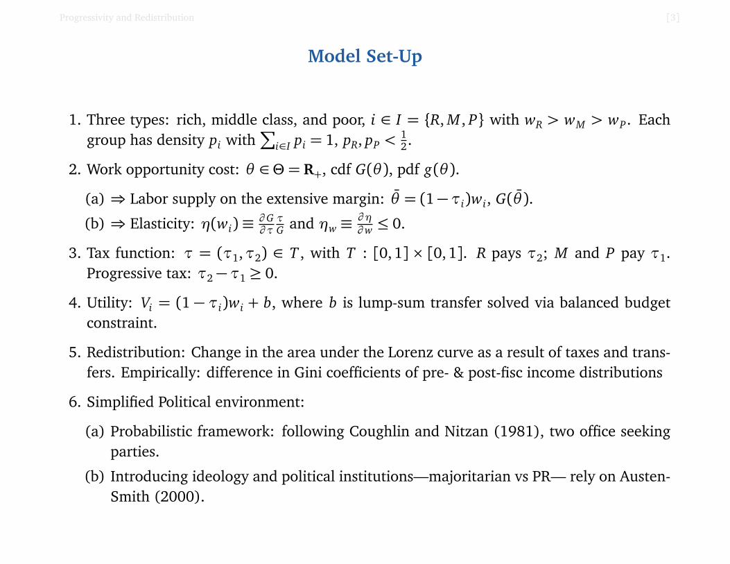
1. Three types: rich, middle class, and poor, i ∈ I = {R, M , P} with wR > wM > wP. Eachgroup has density pi with
∑
i∈I pi = 1, pR, pP <12.
2. Work opportunity cost: θ ∈ Θ = R+, cdf G(θ ), pdf g(θ ).
(a) ⇒ Labor supply on the extensive margin: θ̄ = (1−τi)wi, G(θ̄ ).
(b) ⇒ Elasticity: η(wi)≡∂ G∂ ττG and ηw ≡
∂ η∂ w ≤ 0.
3. Tax function: τ = (τ1,τ2) ∈ T , with T : [0,1] × [0,1]. R pays τ2; M and P pay τ1.Progressive tax: τ2−τ1 ≥ 0.
4. Utility: Vi = (1 − τi)wi + b, where b is lump-sum transfer solved via balanced budgetconstraint.
5. Redistribution: Change in the area under the Lorenz curve as a result of taxes and trans-fers. Empirically: difference in Gini coefficients of pre- & post-fisc income distributions
6. Simplified Political environment:
(a) Probabilistic framework: following Coughlin and Nitzan (1981), two office seekingparties.
(b) Introducing ideology and political institutions—majoritarian vs PR— rely on Austen-Smith (2000).

Progressivity and Redistribution [4]
I: Preferences over Tax Schedules
É Let τ̂i ∈ T be each individual’s group-specific ideal tax schedule.
É Then τ̂R = (τ̂1, 0), τ̂1 ≥ 0, τ̂M = (0, τ̂2), τ̂2 ≥ 0, and τ̂P = (τ̂1, τ̂2), τ̂1, τ̂2 ≥ 0.
É Progressivity of an individual’s ideal tax schedule is nonmonotonic (increasing andthen decreasing) in income. In addition, the level of redistribution implied by an indi-vidual’s ideal tax schedule is decreasing in income.
τ1
τ2
R
PM

Progressivity and Redistribution [5]
II: The Political Process under Income Biased Representation
É Two office-motivated parties, A and B. In this setting, πAi :
πAi = Vi(τA)/(Vi(τA) + Vi(τB))
É Voter from group i more likely to vote for party A if party A’s platform gives greatereconomic utility than party B. All voters vote, so πA
i + πBi = 1. Parties care only about
winning, thus choose platforms, τA and τB, to maximize:
πA=∑
i∈I
πAi .
É As Coughlin & Nitzan demonstrate, this objective is equivalent to maximizing a Nashsocial welfare function:
N(τA) =∑
i∈I
pi ln Vi(τA)
É By assumption: Workers = voters. Unemployed have no weight in the political process
É Equilibrium convergence across platforms
Proposition 1. (Progressive Taxation under Democracy) A symmetric equilibrium tax sched-ule, τ∗ = τ∗A = τ
∗B, exists and is unique. Progressive tax schedules emerge in equilibrium if and
only if there is income inequality.

Progressivity and Redistribution [6]
Inequality, Redistribution, and Progressivity under Income BiasedRepresentation
É Consider a mean-preserving spread in the income distribution from X to Y such thatpX ,P < pY,P, pX ,M > pY,M , and pX ,R < pY,R.
É Then progressivity and redistribution are higher under (more equal) distribution X thanunder distribution Y .
É The mechanisms behind this result are twofold:
1. As the political influence of the rich (middle classes) increases, the level of τ2 de-creases (increases) and the level of τ1 increases (decreases)
2. A higher reliance on τ1 boosts the labor supply reduction by lower income citizensand further reduce the income of M, reducing the pool of revenue available for redis-tribution
É H1: On the marginal effect of tax progressivity on redistribution: For any given level ofeffort and the progressivity of benefits, an increase in the progressivity of taxes doeshave a significant and positive effect on redistribution

Progressivity and Redistribution [7]
III: Political Institutions,Progressivity, and Redistribution
É Suppose that under majoritarian representation, tax policy is coincident with middle-class preferences: τ∗ = τ̂M . Consider now a PR setting (Austen-Smith 2000)
É Then redistribution is higher and progressivity is lower under proportional representationthan under majoritarian representation.
É Plausible reasons:
1. the poor impose their preferences and to maximize revenue reduce the gap in taxburden between R and M
2. the poor and M make a cross-class coalition in which excessively progressive schemesmust give in to minimize behavioral responses and jeopardize the agreement.
3. The idea is to maximize revenue and facilitate redistribution without concentratingthe costs excessively.
É H2: On the relationship between redistribution and tax designs:
1. There is a negative association between the progressivity of the tax system and thelevel of (flat rate) taxation
2. Corollary: as the political influence of the poor increases (PR vs SMD), the ratio ofprogressivity to flat-rate level (proportional) taxation decreases.

Progressivity and Redistribution [8]
Recapitulation: Results and Empirical Implications
É H1 On the marginal effect of tax progressivity on redistribution For any given level of ef-fort and the progressivity of benefits, a change in the progressivity of taxes does have asignificant and positive effect on redistribution
É H2 On the relationship between redistribution and tax designs
1. There is a negative association between the progressivity of the tax system and thelevel of (flat rate) taxation
2. Corollary: as the political influence of the poor increases (PR vs SMD), the ratio ofprogressivity to flat-rate level (proportional) taxation decreases.

Progressivity and Redistribution [9]
Challenges
É Decompose the different elements of progressivity and redistribution empirically
É Reproduce at the micro-level the tax and benefit systems as they are captured by thelegislation
É Capture the intended policy effect, isolating it from the behavioral responses that con-taminate observational data
É Approach: Comparative Microsimulation Analysis

Progressivity and Redistribution [10]
Empirical Strategy and Measurement
É Policy simulation
. Calculation of income effects of tax and benefit policies via OECD TAXBEN model
. For 4 types of households (single, married w/ no, 1, 2 kids)
. At each percentile of income distribution, 50–200% of APW
. Data set with ca. 250,000 cases
É Tax function approach to measure tax progressivity
. Follows clearly from public finance (Feldstein 1969, Persson 1983, Benabou 2002)
. Tax function fit to our income data
T (wi) = wi −λw1−τi
. Mapping of post to pre tax income: x = λw(1−τ)
. τ is direct measure of progressivity
. 1−λ depicts the level of flat rate taxation in the country’s tax function
É Benefit progressivity via Kakwani index
É Redistribution is absolute reduction in (pre-post) Gini of equivalized HH income

Progressivity and Redistribution [11]
Tax and Benefit progressivity
É Substantial cross-national variation
0.05 0.1 0.15 0.2 0.25 0.30
5
10
15
20
25
30
Fre
quen
cy (
%)
Tax progressivity0.4 0.5 0.6 0.7
0
5
10
15
20
25
30
Fre
quen
cy (
%)
Benefit progressivity
É But also within-country variation
Within variance share
Tax progressivity 0.26[0.20, 0.32]
Benefit progressivity 0.13[0.10, 0.17]
Note: Entries are ψe/(ψe +ψu) from mixed model variance decomposition

Progressivity and Redistribution [12]
Statistical specifications
É 203 country-years for 21 OECD countries, 2001–2015
É Unbalanced Panel
É Median years per country: 11
É “Within country” design strategy
. Two-way (country and year) fixed effects
. Within specification
yi t = ατi t + x ′i tβ +φi + ζt + εi t , i = 1, . . . , N , t = 1, . . . , Ti.
. Dynamic panel models (via IV GMM)
yi t = ρ yi,t−1+ατi t + x ′i tβ +φi + ζt + εi t , t = 2, . . . , Ti.
. CRVE (Clustered Robust Standard Errors)

Progressivity and Redistribution [13]
Parameter estimates (H1)T���� IRedistribution as function of spending and progressivity.
(1) (2) (3) (4) (5) (6)Spending levels 0.844 0.842 0.989 0.501 0.476 0.343
(0.119) (0.120) (0.117) (0.070) (0.089) (0.102)Bene�t progressivity −0.036 −0.092 −0.071 −0.131 −0.054
(0.231) (0.196) (0.059) (0.081) (0.093)Tax progressivity 0.439 0.284 0.243 0.229
(0.098) (0.072) (0.091) (0.089)� 0.607 0.534‡ 0.583‡
Two-way �xed e�ects X X X X X X� economic vars. XEstimator FE FE FE FE AR(1) GMM GMM
R-squared† 0.31 0.32 0.44 0.53 0.42 0.54N 203 203 203 182 141 141Note: Unbalanced panel of 21 OECD countries, 2001–2015. All inputs normalized to mean zero and unit standard deviation.
Cluster-robust standard errors.Speci�cations: (1)-(3) Two-way �xed e�ects models (country and year). Average T=10.7. (4) AR(1) model with �xed e�ects
(Baltagi and Wu 1999). (5) LDV model with �xed e�ects (Arellano and Bond 1991; Arellano 2003), GMM IV estimates;estimated on di�erenced system, using lagged LDV and di�erenced covariates as instruments: AR test of residuals p = 0.652.Sargan overidentifying restrictions test: p = 0.162 Speci�cation (6) is (5) with added economic variables (�rst di�erencesin in�ation, real GDP growth, and unemployment rate). AR test p = 0.157, Sargan test p = 0.367. All models include theshare of the 65+ population.
† Refers to “within-panel” R-squared (calculated using doubly demeaned data)‡ Coe�cient on lagged dependent variable.
18

Progressivity and Redistribution [14]
Progressivity and expected value of redistribution
0.40 0.45 0.50 0.55 0.60 0.655
10
15
20
Benefit progressivity
Red
istri
butio
n
A
0.05 0.10 0.15 0.20 0.255
10
15
20
Tax progressivityR
edis
tribu
tion
B
F����� I�e structure of taxes and transfers and redistribution
Expected value (with 95% con�dence intervals) of redistribution at levels of tax progressivity andbene�t progressivity. Based on two-way �xed e�ects model ��ed to panel of 21 OECD countries,2001-2015.
We introduce a lagged dependent variable in column (5) following the speci�cation inequation (17). As expected, we �nd strong persistence of pa�erns of inequality reduction. �eestimate for �, the coe�cient for �it�1, is sizable and statistically di�erent from zero. �us,redistribution in year t is in large parts determined by the amount of redistribution carriedout in year t � 1. In this se�ing, what is the e�ect of a change in the progressivity of the taxand transfer system? Even in this much more involved speci�cation we �nd clear evidence forthe substantive and statistical relevance of the progressivity of a country’s tax structure. �econtemporary e�ect of a unit-change in tax progressivity on redistribution is 0.24 standarddeviations, while the long run e�ect (taking into account both the contemporary change andits feedback via lagged redistribution) is 0.55 (s.e.= 0.22). Finally, this is also con�rmed inspeci�cation (6) where we add variables representing economic conditions that might e�ectachieved redistribution in a mechanical way, namely changes in in�ation, real GDP growthand unemployment.
B. Speci�cation tests
Before we proceed to a discussion of the political signi�cance of our �ndings, we subjectour results to a number of speci�cation tests. We start with a model that allows for hetero-
19

Progressivity and Redistribution [15]
Specification issues
Correlated shocks, endogenous covariates
É Allow common factor(s) Ft with heterogenous impact
É Interactive fixed effectsyi t = ατi t + x ′i tβ + ξ
′iFt + εi t .
É Endogenous covariates (arising from dynamics in unobservables)
x i t = µi + θt +r∑
k=1
akξik +r∑
k=1
bkFkt +r∑
k=1
ckξikFkt +π′iGt +ηi t
Heterogeneity
É Heterogenous α coefficients
É Allow for full heterogeneity in controls and unit-specific time trends
É Pooled Mean Group Estimator (for Ti > 5)
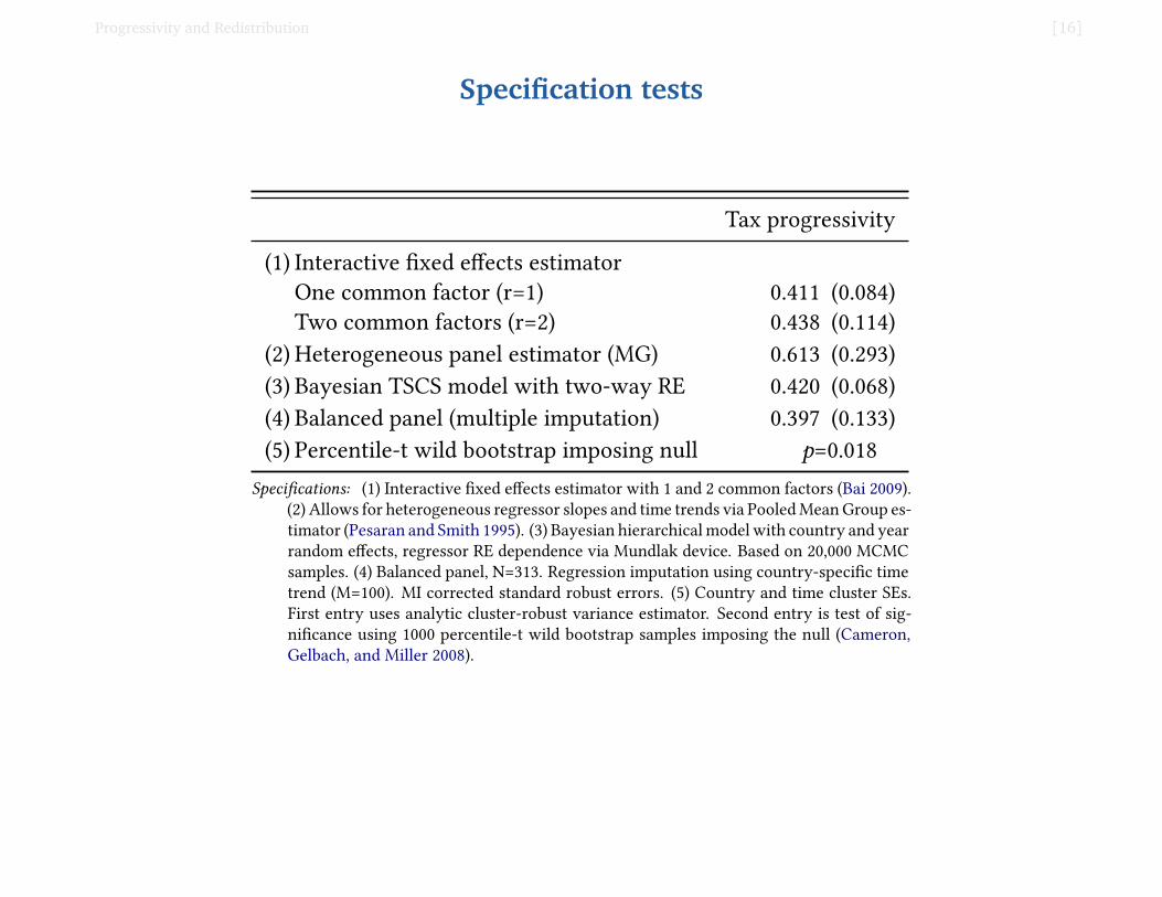
Progressivity and Redistribution [16]
Specification testsT���� IISpeci�cation tests. Estimate of tax progressivity (standard
errors in parentheses).
Tax progressivity
(1) Interactive �xed e�ects estimatorOne common factor (r=1) 0.411 (0.084)Two common factors (r=2) 0.438 (0.114)
(2) Heterogeneous panel estimator (MG) 0.613 (0.293)(3) Bayesian TSCS model with two-way RE 0.420 (0.068)(4) Balanced panel (multiple imputation) 0.397 (0.133)(5) Percentile-t wild bootstrap imposing null p=0.018
Speci�cations: (1) Interactive �xed e�ects estimator with 1 and 2 common factors (Bai 2009).(2) Allows for heterogeneous regressor slopes and time trends via Pooled Mean Group es-timator (Pesaran and Smith 1995). (3) Bayesian hierarchical model with country and yearrandom e�ects, regressor RE dependence via Mundlak device. Based on 20,000 MCMCsamples. (4) Balanced panel, N=313. Regression imputation using country-speci�c timetrend (M=100). MI corrected standard robust errors. (5) Country and time cluster SEs.First entry uses analytic cluster-robust variance estimator. Second entry is test of sig-ni�cance using 1000 percentile-t wild bootstrap samples imposing the null (Cameron,Gelbach, and Miller 2008).
average e�ect of tax progressivity, but leads to increased standard errors (representing theincreased heterogeneity in the model). �at notwithstanding, our core result on the role oftax progressivity is con�rmed.
�e �nal three speci�cations are more technical in nature. In (3) we estimate our modelin a Bayesian framework providing partial pooling estimates for both country and timerandom intercepts. See Shor et al. (2007) for the advantages of Bayesian inference with TSCSdata. We account for regressor random e�ect dependence in both dimensions using theMundlak speci�cation (Rendon 2012).27 We �nd li�le change in our substantive results. Inspeci�cation (4) we create a balanced panel (with 313 country-years) by �lling in valuesfor redistribution under a MAR assumption. Missing years are primarily the results of lackof household panel data in the OECD Income Distribution database, making it more likelythat the missingness process is not MNAR. Note that we have complete information on allyears for our measures of progressivity, as well as for social spending and the share of theelderly. We create 100 imputed data sets and adjust our standard errors for the increase in
both dimensions (N and T) and thus our speci�cation should be seen as providing suggestive only onheterogeneity only.
27We choose non-informative priors with mean zero and variance 100 for all regression type parameters.Variance priors are inverse gamma with shape and scale parameters set to 0.005.
21

Progressivity and Redistribution [17]
Exploring further implications (H2)
É (Negative) relationship between progressivity (τ) and flat-rate tax parameter (1−λ)
É τ/λ ratio in majoritarian and proportional electoral systems
r=0.716, p=0.000r=0.716, p=0.000r=0.716, p=0.000r=0.716, p=0.000r=0.716, p=0.000r=0.716, p=0.000r=0.716, p=0.000r=0.716, p=0.000r=0.716, p=0.000r=0.716, p=0.000r=0.716, p=0.000r=0.716, p=0.000r=0.716, p=0.000r=0.716, p=0.000r=0.716, p=0.000r=0.716, p=0.000r=0.716, p=0.000r=0.716, p=0.000r=0.716, p=0.000r=0.716, p=0.000r=0.716, p=0.000r=0.716, p=0.000r=0.716, p=0.000r=0.716, p=0.000r=0.716, p=0.000r=0.716, p=0.000r=0.716, p=0.000r=0.716, p=0.000r=0.716, p=0.000r=0.716, p=0.000r=0.716, p=0.000r=0.716, p=0.000r=0.716, p=0.000r=0.716, p=0.000r=0.716, p=0.000r=0.716, p=0.000r=0.716, p=0.000r=0.716, p=0.000r=0.716, p=0.000r=0.716, p=0.000r=0.716, p=0.000r=0.716, p=0.000r=0.716, p=0.000r=0.716, p=0.000r=0.716, p=0.000r=0.716, p=0.000r=0.716, p=0.000r=0.716, p=0.000r=0.716, p=0.000r=0.716, p=0.000r=0.716, p=0.000r=0.716, p=0.000r=0.716, p=0.000r=0.716, p=0.000r=0.716, p=0.000r=0.716, p=0.000r=0.716, p=0.000r=0.716, p=0.000r=0.716, p=0.000r=0.716, p=0.000r=0.716, p=0.000r=0.716, p=0.000r=0.716, p=0.000r=0.716, p=0.000r=0.716, p=0.000r=0.716, p=0.000r=0.716, p=0.000r=0.716, p=0.000r=0.716, p=0.000r=0.716, p=0.000r=0.716, p=0.000r=0.716, p=0.000r=0.716, p=0.000r=0.716, p=0.000r=0.716, p=0.000r=0.716, p=0.000r=0.716, p=0.000r=0.716, p=0.000r=0.716, p=0.000r=0.716, p=0.000r=0.716, p=0.000r=0.716, p=0.000r=0.716, p=0.000r=0.716, p=0.000r=0.716, p=0.000r=0.716, p=0.000r=0.716, p=0.000r=0.716, p=0.000r=0.716, p=0.000r=0.716, p=0.000r=0.716, p=0.000r=0.716, p=0.000r=0.716, p=0.000r=0.716, p=0.000r=0.716, p=0.000r=0.716, p=0.000r=0.716, p=0.000r=0.716, p=0.000r=0.716, p=0.000r=0.716, p=0.000r=0.716, p=0.000r=0.716, p=0.000r=0.716, p=0.000r=0.716, p=0.000r=0.716, p=0.000r=0.716, p=0.000r=0.716, p=0.000r=0.716, p=0.000r=0.716, p=0.000r=0.716, p=0.000r=0.716, p=0.000r=0.716, p=0.000r=0.716, p=0.000r=0.716, p=0.000r=0.716, p=0.000r=0.716, p=0.000r=0.716, p=0.000r=0.716, p=0.000r=0.716, p=0.000r=0.716, p=0.000r=0.716, p=0.000r=0.716, p=0.000r=0.716, p=0.000r=0.716, p=0.000r=0.716, p=0.000r=0.716, p=0.000r=0.716, p=0.000r=0.716, p=0.000r=0.716, p=0.000r=0.716, p=0.000r=0.716, p=0.000r=0.716, p=0.000r=0.716, p=0.000r=0.716, p=0.000r=0.716, p=0.000r=0.716, p=0.000r=0.716, p=0.000r=0.716, p=0.000r=0.716, p=0.000r=0.716, p=0.000r=0.716, p=0.000r=0.716, p=0.000r=0.716, p=0.000r=0.716, p=0.000r=0.716, p=0.000r=0.716, p=0.000r=0.716, p=0.000r=0.716, p=0.000r=0.716, p=0.000r=0.716, p=0.000r=0.716, p=0.000r=0.716, p=0.000r=0.716, p=0.000r=0.716, p=0.000r=0.716, p=0.000r=0.716, p=0.000r=0.716, p=0.000r=0.716, p=0.000r=0.716, p=0.000r=0.716, p=0.000r=0.716, p=0.000r=0.716, p=0.000r=0.716, p=0.000r=0.716, p=0.000r=0.716, p=0.000r=0.716, p=0.000r=0.716, p=0.000r=0.716, p=0.000r=0.716, p=0.000r=0.716, p=0.000r=0.716, p=0.000r=0.716, p=0.000r=0.716, p=0.000r=0.716, p=0.000r=0.716, p=0.000r=0.716, p=0.000r=0.716, p=0.000r=0.716, p=0.000r=0.716, p=0.000r=0.716, p=0.000r=0.716, p=0.000r=0.716, p=0.000r=0.716, p=0.000r=0.716, p=0.000r=0.716, p=0.000r=0.716, p=0.000r=0.716, p=0.000r=0.716, p=0.000r=0.716, p=0.000r=0.716, p=0.000r=0.716, p=0.000r=0.716, p=0.000r=0.716, p=0.000r=0.716, p=0.000r=0.716, p=0.000r=0.716, p=0.000r=0.716, p=0.000r=0.716, p=0.000r=0.716, p=0.000r=0.716, p=0.000r=0.716, p=0.000r=0.716, p=0.000r=0.716, p=0.000r=0.716, p=0.000r=0.716, p=0.000r=0.716, p=0.000r=0.716, p=0.000r=0.716, p=0.000r=0.716, p=0.000r=0.716, p=0.000r=0.716, p=0.000r=0.716, p=0.000r=0.716, p=0.000r=0.716, p=0.000r=0.716, p=0.000r=0.716, p=0.000r=0.716, p=0.000r=0.716, p=0.000r=0.716, p=0.000r=0.716, p=0.000r=0.716, p=0.000r=0.716, p=0.000r=0.716, p=0.000r=0.716, p=0.000r=0.716, p=0.000r=0.716, p=0.000r=0.716, p=0.000r=0.716, p=0.000r=0.716, p=0.000r=0.716, p=0.000r=0.716, p=0.000r=0.716, p=0.000r=0.716, p=0.000r=0.716, p=0.000r=0.716, p=0.000r=0.716, p=0.000r=0.716, p=0.000r=0.716, p=0.000r=0.716, p=0.000r=0.716, p=0.000r=0.716, p=0.000r=0.716, p=0.000r=0.716, p=0.000r=0.716, p=0.000r=0.716, p=0.000r=0.716, p=0.000r=0.716, p=0.000r=0.716, p=0.000r=0.716, p=0.000r=0.716, p=0.000r=0.716, p=0.000r=0.716, p=0.000r=0.716, p=0.000r=0.716, p=0.000r=0.716, p=0.000r=0.716, p=0.000r=0.716, p=0.000r=0.716, p=0.000r=0.716, p=0.000r=0.716, p=0.000r=0.716, p=0.000r=0.716, p=0.000r=0.716, p=0.000r=0.716, p=0.000r=0.716, p=0.000r=0.716, p=0.000r=0.716, p=0.000r=0.716, p=0.000r=0.716, p=0.000r=0.716, p=0.000r=0.716, p=0.000r=0.716, p=0.000r=0.716, p=0.000r=0.716, p=0.000r=0.716, p=0.000r=0.716, p=0.000r=0.716, p=0.000r=0.716, p=0.000r=0.716, p=0.000r=0.716, p=0.000r=0.716, p=0.000r=0.716, p=0.000r=0.716, p=0.000r=0.716, p=0.000r=0.716, p=0.000r=0.716, p=0.000r=0.716, p=0.000r=0.716, p=0.000r=0.716, p=0.000r=0.716, p=0.000r=0.716, p=0.000r=0.716, p=0.000r=0.716, p=0.000r=0.716, p=0.000r=0.716, p=0.000r=0.716, p=0.000r=0.716, p=0.000r=0.716, p=0.000r=0.716, p=0.000r=0.716, p=0.000r=0.716, p=0.000r=0.716, p=0.000r=0.716, p=0.000r=0.716, p=0.000r=0.716, p=0.000r=0.716, p=0.000r=0.716, p=0.000r=0.716, p=0.000r=0.716, p=0.000r=0.716, p=0.000r=0.716, p=0.000r=0.716, p=0.000r=0.716, p=0.000r=0.716, p=0.000r=0.716, p=0.000
−20
−15
−10
−5
0
0.05 0.10 0.15 0.20 0.25τ
1−λ
At=2.93, p=0.004t=2.93, p=0.004
2.5
3.0
3.5
4.0
Majoritarian ProportionalElectoral system
τλ
B
F����� IIEmpirical illustration of model implications
Panel (A) plots the relationship between progressivity and �at-rate tax parameter. Superimposed is alowess smoother with 95% con�dence bands. Panel (B) shows the average value of �/� in majoritarianand proportional electoral systems. Error bars represent 95% con�dence intervals.
ted declines, eventually yielding a relatively smaller pool of revenues to be shared. Our�ndings in panel A display a pa�ern that is consistent with this logic on the basis of new,and more precise, measurement strategy.
If su�ciently high redistribution comes at the expense of a partial sacri�ce of progressivity,it should follow that in democracies where political institutions (PR) facilitate strongerpolitical in�uence by the poor, the ratio between � and 1 � � is lower. To address thiscorollary directly, panel (B) plots the average (and 95% con�dence intervals) of the ratio ofprogressivity to � in majoritarian versus PR electoral systems.29 In line with our theoreticalexpectations, in countries with majoritarian electoral systems we �nd the ratio to be 0.80(±0.22) points greater than in countries relying on proportional representation.
VII. C���������What governs the relationship between progressive taxation and redistribution? A
layman’s view would suggest that both are one and the same. And yet, the dominant view
29We exclude mixed electoral systems in this calculation. However, note that including them in the referencegroup does not substantively alter our �nding.
23

Progressivity and Redistribution [18]
Discussion
É Redistribution and Progressivity: A relationship driven by political influence
É Two Faces of Progressivity
É Next Steps:
1. Need to explore conditional relationships suggested by the argument
2. Unexplored Comparative Statics- Endogenous Progressivity as a function of Inequalityand Representation
3. Change the focus: general patterns vs unpacking groups and tools

Progressivity and Redistribution [19]
T���� B.2Summary of estimated tax function parameters
Country � [⇥100] �
Australia 17.73 5.51Austria 17.38 5.53Belgium 21.96 8.79Canada 19.60 7.52Denmark 21.23 10.78Finland 14.82 3.61France 6.71 1.85Germany 15.12 4.53Greece 19.83 7.15Iceland 19.88 19.97Ireland 17.99 6.00Japan 7.98 3.22Netherlands 24.45 11.49New Zealand 10.51 2.48Norway 16.40 6.72Portugal 12.49 3.25Spain 13.96 3.84Sweden 19.76 9.07Switzerland 13.03 4.85United Kingdom 13.76 3.49United States 10.88 2.89
Pooled mean 15.97 6.31Pooled std.dev. 4.84 4.58Within-country std.dev. 1.55 2.14
Note: Parameter estimates of equation 13, 2001–2015 averages. Within-country std.dev. calculated on �it � �̄i + ¯̄� (mutatis mutandis for �).
34

Progressivity and Redistribution [20]
B. E�������� �������Table B.1 shows countries and years included in our analysis. In many cases, the limiting
factor is information on inequality indices needed to calculate our measure of redistribution.Note that we conduct a robustness using multiple imputation (assuming that the processleading to missing inequality information in a given year is MAR) and found no substantivedi�erence in results (see Table II).
T���� B.1Countries and years included in our analysis
Country Years included in analysis
Australia 2004, 2008, 2010, 2012, 2014Austria 2007–2015Belgium 2004–2015Canada 2001–2015Denmark 2005–2014Finland 2001–2015France 2005, 2008, 2009–2015Germany 2004, 2008, 2009-2014Greece 2004–2015Iceland 2004-2014Ireland 2005–2014Japan 2003, 2006, 2009, 2012Netherlands 2005–2014New Zealand 2003, 2008, 2009, 2011, 2012, 2014Norway 2004, 2008, 2009-2014Portugal 2004–2015Spain 2007–2015Sweden 2004, 2008, 2009-2015Switzerland 2009, 2011, 2013, 2014United Kingdom 2001–2015United States 2005, 2008, 2009–2015
Table B.2 shows average tax function parameter estimates (across all years). Besides theclear di�erences in tax structures between countries, it also shows substantial over-timevariation within countries: while the pooled standard deviation for � is 4.8, the within countrystandard deviation is 1.6; for � the overall standard deviation is 4.6 with an within-countrySD of 2. We employ this within-country variation in our empirical analysis.
33

Progressivity and Redistribution [21]
Semi-parametric evidence for impact of τ
−2
−1
0
1
2
0.075 0.100 0.125 0.150 0.175 0.200 0.225 0.250
Tax progressivity (τ)
f(τ)
Related Documents