Productivity and Efficiency Measurement in Agriculturegsars.org/wp-content/uploads/2017/02/TR-17.02.2017-Productivity... · Productivity and Efficiency Measurement in Agriculture

Productivity and Efficiency

Measurement in Agriculture

Literature Review and Gaps

Analysis

Technical Report Series GO-19-2017

February 2017

Productivity and Efficiency

Measurement in Agriculture

Literature Review and Gaps

Analysis

Table of Contents

Preface......................................................................................................................... 5

Acknowledgements………………………………………………………………………………………………... 6

1. Introduction and purpose....................................................................................... 7

2. Basic definitions and concepts................................................................................ 10

2.1 What is agricultural productivity?...................................................................... 10

2.2 Total factor productivity and partial productivity.............................................. 14

2.3 Technical efficiency............................................................................................ 16

2.4 Economic efficiency and competitiveness......................................................... 19

3. Measuring productivity in agriculture.................................................................... 24

3.1 Measuring agricultural output........................................................................... 24

3.2 Quality-adjusted inputs in agricultural productivity measurement .................. 26

3.3 Land productivity............................................................................................... 27

3.4 Labour productivity............................................................................................ 31

3.5 Capital productivity............................................................................................ 35

3.6 Productivity of intermediate inputs................................................................... 39

3.7 Aggregation of productivity indicators............................................................... 40

4. Measuring technical efficiency in agriculture ........................................................ 46

4.1 Introduction........................................................................................................ 46

4.2 Measuring and decomposing productivity growth using Malmquist indices..... 47

4.3 Superlative indices numbers.............................................................................. 49

4.4 Data Enveloping Analysis.................................................................................... 49

4.5 Parametric approaches to efficiency measurement.......................................... 52

5. Agricultural productivity and farm incomes........................................................... 58

5.1 Productivity and farm incomes........................................................................... 58

5.2 Labour productivity and farm incomes.............................................................. 59

5.3 Land productivity and farm income................................................................... 62

5.4 Capital productivity and farm incomes.............................................................. 63

6. United States Department of Agriculture productivity measures: a case study... 65

6.1 Introduction........................................................................................................ 65

6.2 Productivity measurement................................................................................. 65

6.3 Analytical issues.................................................................................................. 69

6.4 Dissemination..................................................................................................... 70

6.5 Quality assessments and improvements............................................................ 70

6.6 Conclusion.......................................................................................................... 70

7. Conclusion................................................................................................................ 71

References................................................................................................................... 73

List of Figures, Tables and Boxes

Figures

1 – Technical efficiency and productivity: an illustration............................................ 19

2 – Economic efficiency: an illustration....................................................................... 20

3 – Construction of the production frontier using Data Envelop Analysis.................. 50

Tables

1 – Characteristics of Labour Input for productivity measurement (USDA-ERS)........ 32

2 – Capital measurement methods of the OECD Capital Manual............................... 37

Boxes

1 – The Malmquist productivity index and its decomposition.................................... 48

2 – Determining the best-practice frontier using data envelopment analysis............ 51

3 – Measuring and explaining technical efficiency of rice growers in Mali................. 57

5

Preface

This literature review and gaps analysis is undertaken in the context of the

research line on the measurement of agricultural productivity and efficiency of

the Global Strategy to Improve Agricultural and Rural Statistics.

It seeks to define the different concepts and present the main measurement

methods for agricultural productivity and efficiency. It does not intend to

provide an exhaustive and detailed description of each method and its

theoretical grounding. Instead, this review and gaps analysis focuses on the

most common ones, identifying the challenges associated with implementation

of them, especially with respect to data requirements.

This activity, as with all the other research lines of the Global Strategy, is aimed

at improving the capacity of developing countries in the provision of quality

statistics on the agricultural and rural sector for which productivity is a

significant and policy-relevant domain. In this perspective, the present literature

review focuses on the challenges of productivity and efficiency measurement

faced by developing countries, which, as many authors have pointed out, have

led to missed estimates of overall agricultural productivity and its driving

factors. This review relies as much as possible on studies and papers that have

focused on developing countries, providing concrete examples of the

implementation of productivity and efficiency measurement.

6

Acknowledgements

The present document has been prepared by Aicha Mechri, Peter Lys and

Franck Cachia, International Consultants for the Global Strategy to Improve

Agricultural and Rural Statistics at the Statistical Division of the Food and

Agriculture Organization of the United Nations (FAO).

We are greatly indebted to the members of the Expert Group on Agricultural

Productivity and Efficiency Measurement, who reviewed intermediate versions

of this document and provided extremely relevant comments, suggestions and

corrections.1

We would also like to thank Flavio Bolliger, Research Coordinator of the

Global Strategy, for providing essential guidance on the content and structure of

this literature review and gaps analysis and for reviewing in detail the

intermediate drafts.

All remaining errors are of the sole responsibility of the authors of this

document.

1 Special thanks to Sun Lin Wang, Keith Fuglie and Richard Nehring from the USDA-ERS,

Patrick Chuni from the Central Statistics Office of Zambia, Martin Beaulieu and Weimin Wang

from Statistics Canada, Rauschan Bokusheva from OECD and Sergio Gomez y Paloma, Pascal

Tillie, and Kamel Louhichi from the EU-JRC, for their participation to the workshop that was

held in Washington D.C. in December 2016 and for their contributions to the literature review.

7

1

Introduction and Purpose

Agricultural productivity and efficiency is at the centre of many of the debates,

policies and measures concerning the farming sector. The emphasis placed by

the Sustainable Development Goals on agricultural productivity underlines the

many reasons for which additional research on statistical frameworks for

productivity and efficiency targeted to developing countries is necessary.

Information on agricultural productivity is related to several of the Sustainable

Development Goal indicators, in particular:

Indicator 2.3.1: Volume of production per labour unit by classes of

farming/pastoral/forestry enterprise size;

Indicator 2.3.2: Average income of small-scale food producers, by sex

and indigenous status;

Indicator 2.4.1: Proportion of agricultural area under productive and

sustainable agriculture.

In parallel to global initiatives, such as the 2030 Agenda for Sustainable

Development, several countries have introduced policies to improve

agricultural productivity, especially in countries where agriculture is a major

economic sector and the productivity gap among the primary sector and other

industries and services is the widest. Enhancing productivity in agriculture is

important because of its effective contribution to poverty reduction through

better food security and higher farm incomes.

The central role of agricultural productivity in the economic and social agenda

of developing countries was reinforced by the Malabo Declaration of June

2014,2 which puts agricultural productivity growth at the centre of the objective

of Africa to achieve agriculture-led growth and fulfil its targets on food and

nutrition security. In the Declaration, it is stated that in order to end hunger in

Africa by 2025, at least a doubling of agricultural productivity is needed from

current levels.

2 The Malabo Declaration on Accelerated Agricultural Growth and Transformation for Shared

Prosperity and Improved Livelihoods (26-27 June, 2014).

8

In this context, proper statistical frameworks are required to monitor progress

towards achieving national, regional or global targets on agricultural

productivity. Research on the measurement of agricultural productivity is not

new and can be traced back to the classical theory of economic growth. More

recently, Solow (1957), Diewert (1980), Ball et al. (1997); Ball & Norton

(2002), among many others, have made essential contributions towards

developing a better understanding, measuring and analysing agricultural

productivity. To the best of the authors’ knowledge, however, only a small part

on this wide body of research specifically addresses the challenges faced by

developing countries in collecting the basic data and in implementing the

appropriate approaches to compile nationwide indicators of agricultural

productivity and efficiency. The weak statistical infrastructure, lack of

appropriate data collection protocols and insufficient surveys and censuses in

these countries limit the availability and quality of data on agricultural

productivity. Among the weaknesses of agricultural statistics in developing

countries, Kelly et al. (1996) identified the underestimation of output, yields

and labour productivity as the most prominent ones.

In addition to addressing basic data requirements, there is need to better define

and measure concepts related to productivity, such as technical and economic

efficiency. Productivity measurement has traditionally assumed the inexistence

of technical inefficiencies in the production process. Starting with Nishimizu &

Page (1982), followed by Fare et al. (1989), the research community has been

placing additional emphasis on the decomposition of productivity changes into

a technological change component and an efficiency component. This

distinction is important. As noted by Grosskopf (1993), if inefficiencies exist

and are ignored in the measurement of productivity, productivity growth no

longer necessarily tells us about technical change and the policy decisions

based on these indicators may be flawed. A better understanding and

measurement of efficiency in agriculture is required in the context of lower

availability of key resources and production factors, such as land or water in

adequate quantity and quality.

Another topic that, to the best of the authors’ knowledge, has not been widely

researched is the description and quantification of the link between productivity

and farm incomes. Indicators measuring the impact of productivity gains on

income generation and food security are useful for policy-making and

monitoring, especially in developing countries where smallholders and family

farms are predominant. In this perspective and given the predominance of

labour among the production costs of these farms, adequately measuring the

9

productivity of labour provided by the farm holder and household members and

its impact on household incomes should be the priority.

The research line of the Global Strategy on “Measuring agricultural

productivity and efficiency” seeks to contribute to the reduction of these

methodological and data gaps. To this end, cost-effective data collection and

computation methods will be identified and field-tested in selected developing

countries. The objective will be to produce operational guidelines and training

material to help developing countries produce data and indicators on

agricultural productivity and efficiency.

This research starts with a literature review and gaps analysis on agricultural

productivity and efficiency. Its first objective is to provide clear definitions of

essential concepts, such as agricultural productivity and efficiency, often used

as synonyms although they cover different dimensions (section 2). Section 3

reviews the main approaches for measuring the productivity of agricultural

inputs and production factors, from the farm-level to sector or economy-wide

scales. By doing this, the document also provides some insights on how to

properly account for the farm outputs, the numerator of any productivity

measure. Section 4 reviews how technical efficiency is defined and measured in

the literature, at farm and aggregate levels. Section 5 explains how agricultural

productivity and farm incomes can be related and how this relationship can vary

depending on the type of holding. Section 6 illustrates some of the

methodologies and approaches described in the literature through the example

of the United States of America, which, to some extent, can be considered as

the gold standard in terms of productivity measurement. Section 7 concludes.

10

2

Basic Definitions and

Concepts

2.1. What is agricultural productivity?

A general definition

“Productivity is commonly defined as a ratio of a volume measure of output to

a volume measure of input use” (OECD 2001b). At its most fundamental level,

productivity measures the amount produced by a target group (country,

industry, sector, farm or almost any target group) given a set of resources and

inputs.

Productivity can be measured for a single entity (farm, commodity) or a group

of farms, at any geographical scale. The measure should reflect the ultimate

purpose for the inquiry. If for example, the purpose is to compare productivity

between farms, then measures that are micro-based are required. If the need is

to evaluate national agricultural policy at the country level, then macromeasures

are required. This same analogy can extend beyond the sector to the national

economy. While the desired purpose can vary, the measurement issues

associated with deriving the different indicators are the same. However, data

requirements may differ depending on the type of indicator: farm-level

productivity measurement for one commodity and one input (for example,

labour productivity of maize farms) may only require basic information on

output quantities and input use, while producing aggregated measures generally

requires pricing outputs and inputs.

Similar to most indicators, a single statistic rarely, if ever, tells a complete story

to provide policy-makers and analysts with sufficient information to

unambiguously prescribe the best policy. For example, a productivity measure

for agriculture that is often cited is crop output per land area (commonly

referred to as crop yield), with a higher yield corresponding to higher

productivity. It quickly becomes apparent that the challenge with this and

similar measures rests with how they are interpreted. Continuing with this

example, a higher yield may be indicative of improved fertilization practices

(use of a better fertilizer and/or more efficient application), land of higher

11

quality allocated to the crop, the use of a better-educated workforce or more

efficient use of capital. However, it may also just be explained by basic factors

beyond the farmers control, such as the soil conditions and even the weather.

Discussion

Productivity measurement has its origins in the microeconomics “theory of the

firm” in which, after simplifying assumptions, it can be shown that inputs can

be combined optimally to allocate scarce resources, allowing firms to maximize

profits subject to a cost constraint or to minimize costs subject to an output

constraint. Both will result with an input allocation that is efficient3 or optimal.

Productivity is studied because, through increased productivity, firms (or

industries, or countries) can better allocate scarce resources to other pursuits. It

leads to higher national income by virtue of this reallocation, by more

efficiently using inputs and by reallocating the “surplus” to other endeavours.

Both results stem directly from the analysis of productivity.

In its simplest form, productivity measures describe the relationship between

the production of a commodity — good or service — and the inputs used to

produce that commodity. It can be the relationship between one or more

products and one or more inputs. Either way, all production, sold or not, and all

inputs, whether they are paid for, should be correctly valued.

As productivity measures describe how the transformation of inputs into

products is affected by efficiency and technological change, it follows that

productivity measures are often volume based. However, in some cases,

efficiency and technological change may not be factors behind increased

productivity. One example would be if production were to double in response to

a doubling of output prices caused by an external shock.

Most farms produce multiple commodities with many inputs. While it is

technically possible to define multi-product output in terms of physical measure

(kilogrammes or joules, for example), it is simpler to convert volumes to

monetary values to perform the aggregation. The aggregation of different inputs

is also generally done using values. In this case, productivity change is

measured by comparing the productivity between two periods using the prices

of a fixed reference period. The difference is, therefore, only attributable to

quantity or volume changes and not due to price variations.

3 For a more complete discussion on technical and economic efficiency, see sections 2.3 and

2.4.

12

Levels versus growth rates

The need to take into account the multi-output multi-input nature of agricultural

activities in productivity measurement explains why indicators focus more on

period-to-period changes than on levels, which can be difficult to interpret.

Producing estimates of period-to-period changes has the additional advantage

of minimizing the effect of the measurement errors affecting level estimates,

provided that measurement techniques and sources remain constant. This results

in a more accurate estimate of productivity change. However, while change

estimates are easier to produce and interpret, these calculations bring in some

additional measurement issues related to the choice of proper indices and

weighting strategies.

The study of growth rates and levels is not a frequently researched question in

literature on productivity, mostly for the reasons presented above. Nonetheless,

completing traditional productivity growth measures with information on levels

may be relevant for several reasons. First, would be for international

comparability purposes. Countries that have already reached high levels of

productivity have less room for additional substantial productivity

improvements, contrary to countries where agriculture is less capitalized,

subsistence-oriented and therefore, where the productivity gap is wide.

Comparing productivity growth of these two groups of countries makes little

sense without additional information on the levels. Second, levels are more

intuitive for single-input (or partial) productivity measures. For example, labour

productivity can easily be measured in levels, such as output per number of

hours or days worked. Levels can be easily compared across subsectors, regions

and countries to provide evidence of differences in input productivity. Some

elements on how productivity levels and growth rates can be constructed at

different levels of aggregation are given in section 3.1.

Farm versus commodity level

Measuring productivity at the commodity level entails collecting plot or

activity-level data on a specific output and on the intermediate inputs and

production factors, such as labour, land and capital used in its production.

Measuring productivity at the farm level implies collecting data on all the

outputs produced and on the different inputs and production factors used. In

principle, as productivity is the ratio of outputs to inputs, the quantification of

productivity not only requires a proper assessment of agricultural production for

the main crops or activities of the holding but it also required for the minor ones

13

and for by-products, such as hay used for forage or manure for fertilization. The

lack of proper accounting for secondary crops or by-products has been

identified by Kelly et al. (1996) as one of the major reasons for the

underestimation of agricultural productivity in Africa.

Given that most agricultural holdings tend to produce several outputs using

many inputs, outputs and inputs generally need to be converted into monetary

units for calculating productivity measure, which, in turn, allows for the

aggregation of a variety of them into a common measure. This means, however,

that proper input and output prices must be available and/or estimated. The

presentation of value-based productivity indicators is also needed to compare

productivity levels of two different products. Measuring the physical

productivity (for example, tonnes/hour) allows comparing the productivity of

two farms that are producing the same product, but not for different crops. In

the latter case, it is necessary to refer to the monetary productivity, converting

the volume produced into a gross output measure (per hour worked, for

example).

Differences between agriculture and other sectors in terms of productivity

measurements

In many respects, productivity measurement for agriculture mirrors that for

other industries. Notwithstanding this, there are several characteristics of the

agriculture sector that make it significantly different and, therefore, worthy of

special consideration.

In most countries, agriculture is comprised of a large number of small

enterprises. These small businesses often use unpaid owner and family-supplied

labour. For the productivity analyst, this fact must be accounted for either

explicitly as an adjustment or in the interpretative analysis. The linkages

between an increase in farm labour productivity and farm family income is not

straightforward.

Natural conditions, such as climate patterns or soil characteristics, have a much

greater effect on agriculture than on most other industries. This is not a problem

in itself, but it does mean that the analyst must exercise a degree of caution

when analysing productivity estimates, not only within a country, but also when

making international comparisons. It also means that statisticians seek to collect

data for certain groups or typologies of farms, often based on the agroclimatic

characteristics in which they operate.

14

Agriculture is also a sector in which a significant volume of inputs can,

depending on the farm type, originate from within the sector and even from the

farm itself. Feed is produced and fed to livestock. Seeds can be retained for

subsequent planting. Labour can be exchanged with other farmers. Beyond this,

agriculture outputs are often consumed on the farm, which is a form of income

even if no market transaction takes place. Land, a key capital input, varies

greatly depending on how arable it is, both across one country and within

countries.

None of the foregoing information makes estimating productivity for

agriculture impossible, but it does suggest that care needs to be taken when so

doing. When collecting or analysing data on agriculture, accounting for these

specificities is essential for the analysis to be credible.

2.2. Total factor productivity and partial productivity

Definitions

Multi factor or total factor productivity growth (MFP or TFP) is the change in

production not resulting from a change in all or several inputs, which in

agriculture is usually land, labour and capital. MFP is, therefore, the difference

between production and input changes or what remains after estimating the

contribution of inputs to production change (OECD 2001b). This residual (what

cannot be attributed to a change in the volume of inputs) is often interpreted as

the sum of pure efficiency change, technological change, and measurement

errors.4 MFP is almost exclusively expressed as a variation or as changes

because, given its highly aggregated nature, level measures would have little

meaning. As the Centre for the Study of Living Standards (CSLS) points out,

MFP captures the residual effects of several elements of the production process,

such as improvements in technology and organizations, capacity utilization and

increasing returns to scale, among other factors. It also embeds errors due to the

miss-measurement of inputs and output (de Avillez 2011, p. 16). Productivity

measures can also be used to illustrate how well a single input is used to

produce products and in the case of labour, this is termed labour productivity.

4 “Further, in empirical studies, measured MFP growth is not necessarily caused by

technological change: other non-technology factors will also be picked up by the residual. Such

factors include adjustment costs, scale and cyclical effects, pure changes in efficiency (OECD

2001b) and measurement errors.”

15

This concept is often calculated, but as already shown, it is difficult to interpret.

Improved labour productivity can be the result of improved use of labour, but it

can also be the result of intensified use of other inputs, such as fertilizer or

machinery. Nevertheless, CSLS also argues that “labour productivity is a better

tool for understanding improvements in overall living standards” essentially

because it is unbounded (de Avillez 2011, p. 29)

Discussion: choosing indices to properly measure productivity changes

As previously stated, productivity measures are always volume based, either

expressed in physical quantities, or in constant value terms, implying that

values be adjusted for price change. In order to get real or constant dollar

measures, time series for outputs and inputs as well as for prices are required, or

alternatively required are output and input volume and price indices. Obtaining

the correct price or price indices, in turn, adds significantly to the complexity of

productivity measurement, most of which is related to matching the correct

price (or index) to the product or input. In the case of outputs, the price or index

used needs to consider the different characteristics associated with the product,

especially the quality characteristics that are associated with the observed price.

Using properly constructed price indices has been the focus of much of the

research on productivity because series indices are commonly used.

Over the years, the research has suggested using different price indices for

deflating outputs and inputs, each with different properties and each yielding

different results. Selecting the appropriate one to use is rooted in theory, but

essentially the choice focuses on how well the chosen price index accounts for

substitution bias. It has been shown by Diewert (1976) and countless others,

that superlative indices (those that satisfy certain numeric properties) can

account for this bias, but they have the base constraint (assumption) that the

industry under study operates under perfect competition and with a certain type

of production function. Because of its desirable properties, the Törnqvist index

is often used to measure TFP for a number of reasons. First, the Törnqvist index

is a discrete approximation of the Divisia index, widely believed to be the best

index for measuring economic aggregates because of its capacity to faithfully

represent the underlying production function and invariance property.5 Second,

as the Törnqvist index is a superlative index, it can be related to many

production or cost functions. In particular, it corresponds exactly to a Translog

function. Third, another advantage is that this index is consistent in

5 As the weights of a Divisia index are being changed continuously, the errors of approximation

as the economy moves from one production configuration to another are eliminated.

16

aggregation: constructing subgroup indices and combining them in an aggregate

index yields almost the same result than aggregating all prices and quantities

together.

Discussion: the “gross output” versus “value-added” approaches

Either “gross output” or “value added” estimates can be used to calculate

productivity. Gross output is generally defined as the value of production while

value-added is gross output less intermediate inputs, which is referred to in

national accounts parlance as intermediate consumption. The value-added based

estimate can be used to measure the returns (net revenue) generated by labour,

land and capital, the primary factors of production.

The gross output measure is often used for estimating agriculture productivity

so that the significant contribution of intermediate inputs, such as pesticides,

fertilizers, plant protection products or seeds, to the sector’s productivity

growth can be taken into account. It is well known that the improvements to

intermediate inputs, such as the ones mentioned, have led to improved

production in the agriculture sector. This is the approach followed by the

agriculture productivity programme of the United States Agriculture

Department (USDA), which is often considered the “gold standard” for

agriculture productivity measurement. Section 6 contains a more complete

description of the USDA agriculture productivity programme.

The value-added approach is meaningful for understanding profitability and the

economic returns from factors of production in agriculture, which is required

for measuring the net production of production costs. Value-added is often used

to compare the profitability of the agriculture industry with other industries

because value added estimates for all industries are generally produced on a

consistent basis within a country’s system of national accounts.

2.3. Technical efficiency

Agricultural productivity is usually considered to depict the efficiency of the

production process, as explained previously in this document. However, as

Grosskopf (2002); Nishimizu & Page (1982); Fare et al (1989); and others have

argued, this is true only under the assumption that the farm (or firm) is

technically efficient, arguably a strong assumption. To understand how these

two notions are connected, it is useful to note that agricultural productivity

depends on two components: the type and quality of the inputs used in the

production process; and how well these inputs are combined. The first

17

component represents the production technology while the second refers to the

technical efficiency of the production process.

Productivity improvements are often entirely attributed to efficiency gains, but

this is often incorrect. For example, Ludena (2010) estimates that agricultural

productivity gains over the period 1961-2007 in Latin America and the

Caribbean have been exclusively driven by technological change, while

efficiency changes have actually been negative over the period. These

approximations arise from the lack of a clear understanding of what is technical

efficiency, how it differs from technological change and how it is connected to

productivity.

Agricultural policies tend to focus more on fostering productivity through

technological change than through better use of the existing technology.

However, rebalancing the focus of agricultural policies towards improving

efficiency is necessary in the context of limited availability of natural resources,

such as land and water, and given the necessity to limit the environmental

footprint of agricultural production. Equivalent physical productivity gains and

perhaps even larger economic gains may be expected from better use of existing

technology than from shifting to new technology. The latter may increase

productivity in the short term, but possibly at the expense of higher production

and environmental costs. For example, before advising farmers to adopt

chemical fertilizers (technological change), traditional fertilization methods

involving organic fertilizers and rotations or mixture of crops (technical

efficiency) may be promoted as a way to increase physical productivity and

improve food security and economic profitability. Technical efficiency is

described in detail in the following paragraphs.

The type of inputs and resources that can

be used in the production process defines

production technology. The production

frontier corresponds to the combination of

inputs that generate the maximum

attainable output. Accordingly, the

production frontier is in fact the best

practice frontier (Charnes et al. 1978). It

differs across countries and regions because

of differences in the nature, quality and availability of the inputs, such as soil

quality, precipitation levels and qualification of the workforce. For example,

rice yields in sub-Saharan Africa will probably never reach yields observed in

Production technology is

characterized by the type of

inputs and resources available.

For a given commodity, many

different technologies may exist,

reflecting different economic,

environmental and agronomic

conditions.

18

South-East Asia because soils, rain patterns and other essential inputs have

structurally different characteristics.

The production frontier is reached when available

inputs are used optimally. A farm (holding) that

reaches its production frontier has also reached its

maximum level of technical efficiency. More

formally, following Odhiambo & Nyangito

(2003), an agricultural holding can be considered

as technically inefficient when, given its use of

inputs, it is not producing the maximum possible

output. Equivalently, a holding is technically inefficient when, given its output,

it is using more inputs than necessary. The concept of technical efficiency is

important because it justifies the existence of differentiated productivity targets,

taking into account both the resource and input base (the technology), and the

distance to the most efficient practices: a holding can be efficient in the sense

that it has reached its own potential maximum production, but less productive

than a less efficient farm benefiting from higher quality inputs.

Figure 1, adapted from Ludena (2010), provides a simple illustration of

technical efficiency and how it differs from productivity, strictly speaking. For

the purposes of this example, the very simple case of an agricultural holding

operating with two substitutable inputs, such as labour and machinery, is

considered. Any combination of labour and machinery along the black line

(point A, for example) corresponds to technical efficiency, in the sense that the

farm produces the maximum amount allowed by the technology. The

technology is characterized by aspects such as the type of soil, meteorological

patterns or the type of capital and labour available. The bisecting line (black

line) illustrates the total production or yield reached with the chosen

combination of the two inputs.

The farm currently operates at F1, an inefficient level. To reach the efficiency

frontier, it needs to better use the inputs at its disposal. Consider now a new

technology, characterized by inputs of a better quality, such as richer soils or a

better-trained workforce or machinery that is more efficient. These two

technologies may be found in different countries or regions, characterized by

different resource and input endowments, for example. This production

technology is represented in the figure by the red line: for the same amount of

inputs, a higher production can be reached. However, the fact that the potential

production is higher with this technology does not mean that farms will

necessarily be more efficient. For example, a farm may be operating at its

A farm is technically

inefficient when it does

not produce the

maximum level of output

that can be expected

given the type of

available inputs

19

efficiency frontier with the black technology, but with a lower yield or

production than an inefficient farm F2 benefiting from better technological

conditions (red line) and with a yield/production comprised between A and B.

Figure 1. Technical efficiency and productivity: an illustration

The production frontier is a theoretical concept and, as noted by Sadoulet & de

Janvry (1995), represents the optimal productivity target and has to be

compared to observe productivity to measure the degree of technical efficiency

(or inefficiency) at the farm-level. The measurement of efficiency relies on the

definition of the production frontier which, given the heterogeneity of

conditions and the diversity of environments in which farmers operate, does not

have to be unique. It is likely to vary across agroclimatic environments and

types of farms (subsistence/family farms vs. commercial holdings) or type of

markets targeted (organic or conventional), for example.

2.4. Economic efficiency and competitiveness

Economic efficiency

According to Kelly et al. (1996), an agricultural holding reaches economic

efficiency when the marginal value of the inputs6 is equal to their respective

unit costs: if the marginal value is higher, the holding can earn higher profits by

6 The marginal value of an input is the additional output value generated by the use of one

additional unit of input.

Input 1 (ex: labour)

Input 2 (ex: machinery)

O

F1

A

BF2

20

producing more, thereby becoming more efficient. If the marginal value is

lower, the farm should reduce its production to increase its profits.

Figure 2, adapted from the G20 Meeting of Agricultural Chief Scientists White

Paper (Fuglie et al. 2016) illustrates the process of convergence towards

economic efficiency. The y-axis represents the output value and the x-axis the

inputs costs. The black line indicates how inputs are transformed into outputs:

the points situated on this line indicate that the agricultural holding is operating

at the highest potential yield or production given the type and quality of inputs

used, that is, it is technically efficient. Assuming fixed input and output prices,

any increase in production value for technically efficient holdings (from 𝑉𝐴 to

𝑉𝐵, for example) is due to an increase in the quantity of input used (from 𝐶𝐴 to

𝐶𝐵).

Figure 2 – Economic efficiency: an illustration

The ratio between output value and input value measures the amount of value

generated by one monetary unit of input: in other the words, the economic

return per monetary unit spent. This indicator is also known as unit margins or

profits. The figure illustrates that the additional return generated by an increase

in use of inputs declines as more inputs are being used: the additional value

created by moving from A to B is higher than for the change from B to C and so

on until reaching E. After E, any additional quantity of input used does not

translate into higher output, meaning that the additional return is 0. E can,

therefore, be understood as the point at which the farm is economically

efficient: before E, there is scope to increase the overall profitability by using

more inputs; after E, any additional use of input will result in lower profits. This

is due to the existence of declining returns to scale in agriculture, which is a

21

widely known and observed phenomenon resulting from the fact that yields and

production are bounded by physical constraints. Yields can rise as far as more

inputs are used, but up to a certain point, after which, the use of additional

inputs will have no impact on yields and only result in higher costs.

In practice, a technically efficient farm can be economically inefficient.7 It is

especially true in developing countries where markets are often thin or

inexistent, inputs are constrained (unavailable or difficult to access) and

transaction costs are high. For example, a farm may need to use more of a

certain type of input to reach prescribed technical efficiency targets, but it may

not have an economic interest to do so given the current market conditions

(very high input cost, for example). Information on the marginal productivity of

key inputs as well as on their costs of acquisition is useful in understanding the

production constraints that farmers face and how they might react to certain

stimuli that are regulatory or economic in nature.

Moreover, and perhaps more importantly, the concept of economic efficiency is

largely irrelevant for certain groups of farms, especially farms in which their

main priority is to satisfy the livelihoods of their related household(s). For those

holdings, producing more food may not be an objective if self-sufficiency is

ensured, even if by doing so, they would achieve higher economic returns.

Conversely, agricultural households that are not producing enough to satisfy

their needs cannot envisage reducing output to maximize economic efficiency.

This does not mean that the analysis of farms through the prism of economic

efficiency should be theoretically limited to commercial farms. First, because

having information on the underlying economic profitability of subsistence

farms is useful to understand how profitable farming may be compared to other

potential activities. Second, because the dividing line between commercial and

subsistence farming is not clear-cut: farms may run activities that serve

different purposes, such as producing food for the household (for example,

sorghum and millet in sub-Saharan Africa), generating cash revenue (such as

cotton and sugar crops) or both (maize and cassava). Furthermore, once the

basic needs of the household are satisfied, subsistence farms may essentially

turn to profit-generating activities.

7 The reciprocal, though, is not true: an economically efficient farm has to also be technically

efficient.

22

Competitiveness

An additional distinction that needs to be made is between economic efficiency

and competitiveness. The former is an absolute measure of the economic

performance of the farm whereas the latter compares this performance to that of

their competitors. In other words, a farm can be economically inefficient but

competitive because other farms are even less efficient. Reciprocally, an

economically efficient farm is not necessarily competitive if all the other farms

are also economically efficient. Competitiveness also goes beyond the

price/cost performance and extends to the features attached to the output or to

the producing firm (or sector, country), such as quality attributes, both true and

perceived. For example, a firm can have comparatively high unit costs but may

benefit from a high “non-price” competitiveness, which allows it to sell its

products at a higher price.

A more precise definition is given by Porter (1990), who differentiates

competitiveness according to the geographical scale:

At the local level, “competitiveness is the ability to provide products

and services more effectively and efficiently than relevant competitors

and to generate, at the same time, returns on investment for

stakeholders”;

At national or regional level, “competitiveness is the ability of

enterprises to achieve sustainable success against their competitors in

other countries, regions or clusters” (Porter, 1990).

Competitiveness is most often measured using economic indicators, such as

gross or net margins (often per unit of land), and comparing the performance of

farms (or farming systems) based on these measures. Competitiveness and

productivity are closely related: higher productivity can lead to a greater

competitiveness of the enterprise (or sector) because more is produced out of

the same amount of resources. This means that, with all things being held equal,

the cost of production per unit of output is lower, and that margins per unit of

output are higher. Productivity is a necessary precondition for competitiveness,

but not a sufficient condition. Indeed, a multitude of factors affecting the

competitiveness of an enterprise has been identified in the literature.

Competitiveness is the result of a combination of factors, both national and

international:

Nationally, resource endowments, technology, productivity, product

features, fiscal and monetary management and finally the trade policy

23

are seen to be the most important factors that determine the

competitiveness of an industry and/or business. Productivity is,

therefore, seen as one of the national (domestic) determinants of

competitiveness;

Internationally, the most important factors are exchange rates,

international market conditions, the cost of international transport and

the preferences and settings between different countries (Porter, 1990).

24

3

Measuring Productivity in

Agriculture

3.1. Measuring agricultural output

Concepts

As productivity is the volume measure of production (output) divided by the

volume measures of inputs,8 it is important to define what is meant by

production or output.

To keep measures of productivity consistent and aligned with economic theory,

production should measure the total output of a specific production process that

combines intermediate inputs and factors of production to create a product. It is

counted if the product is sold for domestic final consumption, including home

consumption by the agricultural household, for export or added to inventories.

Practices for the treatment of products that are used as an intermediate input for

other agriculture production can vary, but whichever method is chosen, it must

ensure that the concept is consistent on both the output and input sides of the

farm accounting balance sheets.

This can be illustrated by way of an example. Suppose a farmer sells grain to a

feed processing mill that, in turn, sells processed feed to a livestock farmer.

Most statistical systems would count the sale from the farm to the mill as a sale

from agriculture (part of output) and the purchase of the feed from the mill as

an intermediate input. Now consider feed grown on the farm that is used for the

farmer’s own livestock. It is common and correct not to count own account feed

as an output if agriculture productivity is being measured. This holds except if

there is an interest to measure crop productivity or livestock productivity

separately. Under that situation, it would be necessary to value gross

commodity flows.

8 The term “volume” means that outputs and inputs are either measured in physical terms or,

most frequently, in value terms, but using the prices referring to a fixed reference period. This

allows interpreting period-to-period changes as changes in volume.

25

Following the above example, output can be measured as the sum of sales plus

own-consumption plus change in inventories. It is also appropriate to measure

livestock inventory change in weight gain and not just by the change in the

number of heads so that the compositional change in the livestock herd can be

better accounted for. As this approach is very data intensive, the number of

head method is mostly used. Using auxiliary information and parameters can

derive weight estimates. Crop production is measured net of harvesting losses

and, if possible, net of other on-farm post-harvest losses, to capture the amount

that is actually available for use or to be sold. Reducing farm losses would

directly translate into higher productivity, as it would lead to higher output with

no additional input cost.

In principle, agricultural output should not include on-farm transformed

production if the expenses associated with those outputs can also be excluded.

Output of transformed products is generally attributed to manufacturing

industries. Countries may, however, opt to include transformed products for

items that require limited transformation, such as milk products, in sectors in

which most of the farm revenue come from selling or consuming these goods,

or if the expenses cannot be clearly separated (the production technologies of

the raw and processed product are joint). The output considered should only

refer to on-farm processing, and any output generated by off-farm processing

should be systematically excluded.

Prices used to value output are market prices at the farm gate. To measure the

underlying productivity, output prices should be net of any subsidies received

or taxes paid. These prices are also referred to as basic prices. When output is

recorded at basic prices, any tax (subsidy) on the product actually payable on

the output is treated as if it were paid (received) by the purchaser directly to the

government instead of being an integral part of the price paid to the producer

(OECD, 2001b). The information on subsidies is, however, useful for

conducting a cost of production and profitability analysis. Own-consumption

should be valued at the price the farmer would have received had the output

been sold rather than consumed, or in other words, the opportunity cost).

Measurement issues

Farming systems in developing countries tend to be fairly diversified. Often,

they combine crops and livestock activities and cash crops with subsistence

activities. Proper accounting of the output of the farm, including secondary

crops, by-products and unsold produce, is a prerequisite for obtaining an

adequate measurement of productivity.

26

The common practice of mixed cropping in developing countries where several

crops are simultaneously grown on the same parcel of land adds complexity to

the measurement of output. Kelly et al. (2016) found that the most important

problem associated with the measurement of productivity in developing

countries, and particularly in sub-Saharan Africa, is the underestimation of

output and yields because secondary crops and by-products are not properly

estimated. An illustration of this is provided by Hopkins and Berry (1994), who

estimated that in Niger, returns to labour (labour productivity expressed in

monetary units) were 20 per cent lower when only the principal crop was

accounted for, as compared to when the output is measured for both the

principal and secondary crops.

The case of horticultural crops is another example of lack of proper accounting

of the crop output. Because of the small area generally occupied by those crops

as compared to cereal or typical cash crops, the corresponding output is

typically not accounted for. This is especially the case when the farmers are just

starting to diversify into such products as fruits and vegetables. The potential

high value and relative importance of revenue generated by horticultural

products make it necessary to include them in the measurement of farm output

(Kelly et al. 1996).

Another source of underestimation of output is the lack of accounting for crops

that serve as inputs to other production processes: if an output is used as input

in another enterprise (the case of hay used for animal feed, for example), it

should be accounted for as an output for the crop enterprise, otherwise, the

measurement of agricultural output, as well as the measures of profitability and

productivity at the micro level are biased (Kelly et al. 1996).

3.2. Quality-adjusted inputs in agricultural productivity

measurement

Agricultural productivity is dependent on the quality of the inputs and how well

those inputs are integrated in the production process. For example, land

productivity highly depends on the location of the land and its physical

characteristics. This is the same for labour as the quality of the work force

differs across, for example worker types or subsectors.

For comparative purposes, the quality of the input must be taken into account in

the data collection and appropriate adjustments need to be made after the data

are collected. This means that data on input use need to be collected for

different types of inputs or quality classes. For example, family labour,

27

occasional workers and permanent workers should be differentiated in the data

collection process. Because workers with different skills have different levels of

productivity, using the same wages for workers with different qualification

levels results in biased estimates of labour productivity. The same applies to

fertilizers or to any other input or production factor that has varying

characteristics. With regard to fertilizers, this input varies in terms of the dosage

of active ingredients to pesticides, which may be more or less effective. One

kilogramme of fertilizer applied in 2000 is not comparable to one kilogramme

applied in 2015, because of two factors: the introduction of new and more

effective products; and fertilizer demand may have shifted towards other

segments of the market. This change in composition should be reflected in

differentiated input prices.

To address the issue of compositional or quality change, sophisticated

frameworks for input quality adjustments have been developed. The United

States Department of Agriculture-Economic Research Service (USDA-ERS),

for example, estimates quality-adjusted wages based on data of hours worked

and wages per hour cross-classified by different labour categories (the

following section on labour productivity provides additional details). For land

productivity, land prices or rents can be imputed using hedonic regressions that

take into account some of the differences in quality attributes, such as soil type,

moisture, soil acidity and salinity. Quality-adjusted prices for other inputs can

be constructed using similar techniques.

Taking into account input quality is crucial for attaining accurate TFP

estimates, but this requires the availability of detailed and accurate datasets on

input quantities, values and prices for different quality classes. This requirement

leads to increased data collection costs and a higher response burden.

3.3. Land productivity

Definition

The productivity of the land measures the amount of output generated by a

given amount of land. It is mostly applicable in the context of cropping

activities, but it can also be extended to livestock production, in certain cases,

as shown below.

There are several productivity measures that can be calculated: a broad measure

is the ratio between the value of all agriculture products (crops and livestock)

and the total land used in agriculture. Other land productivity measures can be

28

calculated by dividing crop production by the amount of planted land,

expressed in an area unit, such as hectares or acres. When expressed in terms of

physical output, such as tonnes of maize, land productivity corresponds to crop

yields. When expressed in monetary terms, land productivity is more often

referred to as returns to land.

Land productivity = Volume of output / Planted Area9

Planted area is used instead of other area concepts, such as harvested area,

because of the interest to measure the effective yield or land productivity rather

than a theoretical or biological yield. The use of inputs prior to the harvest is

made on the sown/planted area (such as fertilizer applications) and not in

reference to the harvested area, which at the pre-harvest phase is usually

unknown. The difference between harvested and planted area may also reflect

the efficiency and relevance of the farming practices, in addition to exogenous

factors, such as climate-related events, which should be reflected in the

productivity indicator. Using harvested area instead of planted area tends to

lead to overestimations of yields and returns to land because this area includes

the most productive segments of the parcel. In general, it is best to use planted

area for a monocropping system and cultivated area, including fallow land, for

mixed cropping systems.

Agricultural production used for the calculation of productivity should include

the production of the crops grown on the same land during the reference period

whether it is one cropping season or one year. This is important because, in

practice, farmers often grow more than one crop on the same plot over a year;

they may grow a mixture of crops on the same plot at the same time or rotate

the crops grown on the plot over the season. Kelly et al. (1996) stressed that one

of the reasons behind the tendency to underestimate output and yields in

developing countries is the lack of accounting of crops grown in mixture or in

sequence and the lack of appraisal of by-products, which may be sold,

consumed by the household or used in the production of other products. It is,

therefore, essential that all crops are included in the measurement of

productivity, especially in developing regions where these practices are

common.

9 Planted area in this context includes permanent crops and the pasture.

29

Measurement issues

Units

As with other inputs, land productivity can be expressed in many units. Given

that the land may be used to grow many different crops, a physical unit, such as

tonnes, may not be the best choice. Putting a monetary value on their respective

output is often needed to aggregate the output of different crops.

Land quality

Productivity measurement should take into account as much as possible soil and

land quality differences by collecting data on the soil/land characteristics and

their related aspects, especially land prices and rents. For example, differences

in the quality of land across states and regions in the United States are reflected

by calculating relative prices of land from hedonic regression results. Ball et al.

(2008) applies a hedonic approach to measure quality-adjusted land prices

assuming land price is a function of characteristics of land quality variables,

such as soil acidity, salinity and hydric stress. The output derived from the land

use depends on the soil and land characteristics. USDA uses a database that

gathers information on those characteristics in different states and regions from

the "World Soil Resources Office". This method, even though it is accurate,

requires a large amount of data that are not necessarily available in developing

countries.

Indeed, land/soil characteristics and yields may not always be linked, as

intuition would suggest, limiting the generalized use of models and other data

imputation tools. For example, Vesterby & Krupa (1993) have shown that soils

of poor physical quality can sometimes produce very high yields.

In addition, land values do not necessarily reflect environmental aspects of soil

quality. In developing countries, for example, land prices may be more closely

related to the existence of irrigation systems on the farm. Usually, irrigation

infrastructure and equipment are measured in the capital input. When

measuring land productivity, it is important to at least identify the percentage of

land that is irrigated in the total land available.

Land productivity and livestock production

Land productivity can also be calculated in relation to livestock activities to the

extent that the land is directly devoted to pasture/grazing or to the cultivation of

30

crops destined to feed the animals, such as hay or silage crops. Land

productivity cannot be calculated for livestock systems fully based on stall-

feeding management.

Land productivity for livestock measures livestock production in terms of

output per unit of land. The type of livestock product (output) of the enterprise

has to be well identified (whether it is, for example, meat, milk, eggs or live

animals). The land productivity is then the volume of the livestock product

(tonnes of beef, for example) divided by the unit of land used for livestock,

especially the land that is devoted to pastures, hay and silage crops.

In mixed livestock and cropping systems, the productivity of land used for

cultivation can increase with the presence of animals because animals

transform nutrients from legumes and pastures and put them back in the soil in

the form of manure and urine, which are organic inputs. In an agricultural

system based only on livestock raising, feed has to be bought from the market

and the waste produced by animals cannot be easily eliminated.

Natural capital and productivity measurement

Productivity measurement should take into account as much as possible the

existence and characteristics of the natural capital. Natural capital is the natural

environment in which the production takes place and comprises such factors as

the quality of the land in terms of natural minerals and fossils composition and

weather patterns (rainfall, temperature and sunlight, among others).

Understanding the role of natural capital for agriculture and their interactions is

essential in determining the environmental sustainability of farming activities,

or their capacity to obtain sufficient yields in the long term without generating

any type of negative externalities to the environment where the production

occurs. The depletion of natural capital may potentially lead to short-term

economic growth or an increase in yields, but this would be at the expense of

future growth if the revenues that are generated from the short-term growth are

not reinvested to maintain or increase the capital base, physical and natural

(Schreyer et al. 2015).

Data on farms should be geo-referenced, to enable the superposing of

information on soils and land coming from other datasets. The same applies to

data on weather patterns. In addition, basic information on the type of soils

should also be collected. Information on practices affecting the environment,

such as manure management or pest control, can also be sought. Collecting and

presenting data for different types of agro ecological zones, the definition of

31

which may be more or less sophisticated depending on data availability, is

necessary for making assessments and comparisons of yields, revenue or input

use between different typologies of natural environments and production

conditions.

Data requirements for land productivity measurement

Output data:

Crop production, including secondary/minor crops and by-products, in

quantities and values;

Number of animals by species;

Livestock production by product in quantities and values.

Input Data:

The total area of land planted for each crop;

The average annual per unit cost of land;

Total area of land available for cropping, namely the sum of cultivated

land for all crops and fallow land;

The share of land used for pasture;

Management system for livestock.

In addition, information on the environment and production conditions, as

described above, should be made available.

3.4. Labour productivity

Definition

Labour productivity in agriculture measures the number of units of output(s)

produced per unit of labour used in the process of production. It is a partial

productivity indicator that is calculated by dividing the quantity of output by the

total units of labour used:

Labour productivity = Volume of output / Units of labour used

There are many ways to assess the quantity of labour input: the number of

workers active on the holding; the number of time units (such as hours, days

and months) worked or full-time equivalent units if an average number of hours

per working day can be determined according to specific country standards.

32

OECD (2001) recommends that labour input be measured using the number of

hours effectively worked. Using the number of hours corrects for the difference

between seasonal and non-seasonal workers and the different working regimes

(part-time versus full-time). This allows better comparisons across production

systems, regions and countries, as the number of workers or of days per worker

may not indicate the labour input effectively used on the farm.

However, the change in the number of hours reported does not always reflect

the use of capital, the quality of the workforce and technology (Shumway et al.

2015). USDA-ERS suggests that productivity measurements capture the

different types of labour working in the sector because labour input differs

based on the categories of workers. It is recommended that distinctions be made

between different ages of workers, family labour and hired labour and men and

women. Distinctions can also be made between part-time and full-time workers.

A distinction should also made between the different educational levels,

because the quality of one hour provided by a worker is often dependant on his

skills and capacities.

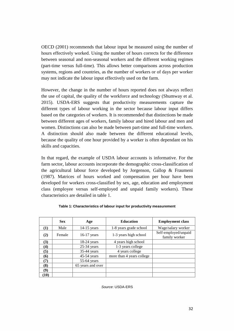
In that regard, the example of USDA labour accounts is informative. For the

farm sector, labour accounts incorporate the demographic cross-classification of

the agricultural labour force developed by Jorgenson, Gallop & Fraumeni

(1987). Matrices of hours worked and compensation per hour have been

developed for workers cross-classified by sex, age, education and employment

class (employee versus self-employed and unpaid family workers). These

characteristics are detailed in table 1.

Table 1: Characteristics of labour input for productivity measurement

Sex Age Education Employment class

(1) Male 14-15 years 1-8 years grade school Wage/salary worker

(2) Female 16-17 years 1-3 years high school Self-employed/unpaid

family worker

(3) 18-24 years 4 years high school

(4) 25-34 years 1-3 years college

(5) 35-44 years 4 years college

(6) 45-54 years more than 4 years college

(7) 55-64 years

(8) 65 years and over

(9)

(10)

Source: USDA-ERS

33

In addition, ERS has developed a set of similarly formatted but otherwise

demographically distinct matrices of labour input and labour compensation by

state. This is accomplished using the Bi-proportional MatrixBalancing (RAS)

procedure popularized by Jorgenson, Gollop, & Fraumeni (1987), which

combines the aggregate farm sector matrices with state-specific demographic

information available from the decennial Census of Population (U.S.

Department of Commerce). The result is a complete state-by-year panel dataset

of annual hours worked and hourly compensation matrices with cells cross-

classified by sex, age, education, and employment class and with each matrix

controlled to the USDA hours-worked and compensation totals, respectively.

Indices of labour input are constructed for each state and the aggregate farm

sector using the demographically cross-classified hours and compensation data.

Labour hours having higher marginal productivity (wages) are given higher

weights in forming the index of labour input than are hours having lower

marginal productivities. Doing so explicitly adjusts the indices of labour input

for “quality” change in labour hours, as originally defined by Jorgenson &

Griliches (1967).

Measurements issues

The accuracy of the labour productivity estimate depends on the quality of the

data in the numerator and the denominator. As mentioned earlier, it is

recommended to measure labour in as much detail as resources and collection

constraints permit, with the ideal being to capture the number of hours or days

per person over a specific period of time, and not as an aggregate, such as the

number of persons employed by the holding. The latter does not inform about

the actual time spent on agricultural activities: for example, full-time, part-time

or seasonal workers do not work the same number of hours per year. Until

recently, many national and international datasets on labour only provided the

number of workers employed by the agricultural sector (Kelly et al. 1996).

However, improvements have been made and data on effective labour input in

agriculture are becoming more readily available. Examples are data on the

average weekly hours actually worked by agricultural employees disaggregated

by sex provided by the International Labour Organization.10

Combined with

information on the number of persons employed in the agricultural sector, it is

possible to estimate the labour input in the agricultural sector, measure labour

productivity and carry out cross-country comparisons. However, data gaps for

several developing countries, especially in Africa and parts of Asia, remain

important.

10

See www.ilo.org/ilostat.

34

Labour productivity is often linked to other factors, such as land and capital.

For instance, as noted by Kelly et al. (1996), farmers in countries where labour

is scarce and land is abundant tend to adopt production systems that provide

high labour productivity. Capital also plays a major role in labour productivity.

In the past 50 years, labour productivity in agriculture has increased because of

the growth in crop yields globally. Roudart & Mazoyer (2006) show that in

some regions of industrialized and emerging countries, yields have been

reaching ten tonnes of cereals or cereal equivalent per hectare, close to the

maximum attainable level. This yield increase is mainly the result of using

genetically improved seeds, with high yield potential, along with an increase in

chemical fertilizers and pesticides use and, in some cases, the intensification of

irrigation. Improvements in labour productivity are also often related to

increased mechanization because machines that are more efficient require less

labour to cultivate a larger area. Therefore, the disparity in estimated labour

productivity across countries and regions can be partially explained by the

wider use of machinery in developed countries in comparison to developing

countries. This illustrates the limitations of partial productivity indicators in

accounting for structural changes in farm inputs and their composition, which

modify the respective contribution of each input to farm productivity.

Relationships between labour productivity and other inputs are further

described in section 5.2. in connection with farm incomes.

Data requirements

Labour quality differs across countries, type of activities, region and many

other dimensions. High-skilled workers produce a different output than low-

skilled workers, which yields very different effects on production (OECD

2001). Taking into account differences in labour quality is important when

labour input is expressed in value terms (wage): failure to differentiate labour

types in the valuation of labour input, for example, using wages for low-skilled

workers to value labour provided by high-skilled labour results in biased

estimates of labour costs and returns to labour. This issue becomes mute when

using a physical measure of labour productivity: if labour quality is higher in

one country and if the number of hours worked are correctly measured, this is

reflected in higher labour productivity for this country (expressed in tonnes per

hour worked, for example).

The increased precision and level of detail in disaggregating different labour

categories, such as age, gender and education, leads to higher data collection

costs, possible response bias and a greater response burden.

35

To summarize, the proper measurement of labour input for productivity

measurement requires a specific type of information, in particular on the

following:

Number of workers per category of workers, including unpaid family

labour;

Characteristics of workers (table 1);

Number of hours worked per agricultural product/activity;

Net wage (cash and in kind payment) per category of worker, including

an estimation of imputed wages for unpaid labour;

Value of any type of compensation or benefits paid for or provided by

the employer, either in cash or in kind, such as pension contributions or

social security.

3.5. Capital productivity

Definition

Capital productivity measures the contribution to production of the capital

employed in the production process. Capital is usually defined as an input

owned by the farm that provides services over several years. When measuring

capital, most productivity measures only focus on farm buildings, machinery

and equipment. Hired and owner-supplied labour is often considered to be a

form of capital (human), but it is commonly measured as labour input (OECD

2001). Tree stock and orchards, as well as livestock can also represent a capital

stock when they result from an investment (purchase of animals or the

establishment of a new plantation, for example) that leads to a regular flow of

revenue or service (revenue from the selling of fruits or milk or service

provided by animal traction, for example). However, given the specificity of

these assets, the fact that the measurement is particularly complex (especially in

developing countries) and the relatively few references on the subject, this

section focuses on traditional assets, such as machinery, equipment and

buildings. Ball & Harper (1990) can be consulted for a specific discussion on

livestock as capital assets.

Capital productivity is computed using the following formula:

Capital productivity = Volume of output / Volume of capital input

Capital input is determined by estimating the service flows stemming from the

capital employed. To estimate capital service, it is necessary to first estimate the

36

stock of productive capital used for each asset type, then determine rental prices

and finally estimate capital service flows.

Capital stock

The capital stock consists of the value of all the fixed assets, such as machinery,

equipment, buildings and other structures, used by the farm, that provide inputs

in the form of capital services into processes of production. The capital stock

can also be viewed as the cumulative value of the past capital investments

made.

To measure capital stock, two approaches are generally used:

Approach 1 - perpetual inventory method (PIM): it involves adding

to the previous year’s stock the estimate of the current year’s new

investment while simultaneously ageing the productive capital by one

year as it is moved forward, a process known as capital depreciation.

Capital depreciation is most often estimated by asset type with farm

buildings and structures depreciated over a much longer time horizon

than farm machinery, reflecting actual service lives. The perpetual

inventory method can, therefore, be formalized as the following:

𝐊𝐭 = 𝐈𝐭 + (𝟏 − 𝛍)𝐊𝐭−𝟏 ; where Kt is the current year’s capital stock,

It current year’s investment, and μ the replacement rate or depreciation

factor.

Approach 2- current inventory method (CIM): it is based on a count

and valuation, sometimes adjusted for the estimated average age of

capital goods, of the set of capital goods being used on a farm.

Although the perpetual inventory method is mostly used to estimate

capital stock, it requires an important set of data, unlike the current

inventory method.

The choice of the method (PIM or CIM) depends on the data collected and

available. If macrolevel total factor productivity is measured, then using the

PIM method for capital is a first best approach, unlike its application in

micromeasures.

Capital investment is depreciated by using a formula mostly because robust

market prices for age-type capital goods generally do not exist. Various

methods can be used to depreciate capital. Each one depicts the service life of a

capital asset. The straight-line method assumes that a capital asset will provide

37

constant service for a set number of years. The hyperbolic formula infers that

the service falls off less when the asset is new and more when it is old. For all

of the methods, a somewhat arbitrary service life for the asset must be selected.

The OECD Manual on Capital Stock Measurement gives detailed examples of

the capital measurements methods, which are summarized below.

Table 2: Capital measurement methods of the OECD Capital Manual

Type of age-efficiency or age-price profile

One-hoss-hay (O) or

hyperbolic (H) Straight-line

Geometric

User cost

weights

Market price

as weight

User cost

weights

Market

price as

weight

User cost

weights

Market

price as

weight

Fixed-weight

index

number

Typical “gross

stock” measure

in OECD countries (O)

The Statistics

Canada’ net

capital stock

measure with

hyperbolic

depreciation profile

Typical

“net” capital

stock

measure in

OECD

countries

The Statistics Canada

MFP capital input measure

Flexible

weight index

number

(for example,

Fisher,

Tornqvist

indices)

The U.S.

Bureau of

Labour

Statistics’

Capital

services

measure (H)

Australian

Bureau of

Statistics’

capital

service

measure (H)

The Australian

Bureau of

Statistics net

capital stock

measure (age-

price profile

based on

hyperbolic age-

efficiency profile)

Jorgenson

(1989) 11measure

of capital services

The U.S.

Bureau of

Economic

Analysis

Fixed

Reprod ucible

Tangible

Wealth

measure

Source: OECD (2001b).

11

Jorgenson, D., 1989. Productivity and Economic Growth. Ernst R. Berndt and Jack E. Triplett

(eds.), Fifty Years of Economic Measurement, University of Chicago Press.

38

Rental prices

After the capital stock is determined, the next step is to place a value on the

capital that was used in the year. This value is most often referred to as rental

prices, given that capital is often rented. and rental values tend to be more easily

observed than actual asset prices. In addition, rental prices include depreciation

rates of capital goods.

In the case of an existing rental market (for agricultural machinery, for

example) the price of the capital service is measured as its rental price.

However, rental markets are thin or inexistent for many capital goods,

especially in developing countries. In this case, their rental price can be imputed

based on an opportunity cost of the capital, or more commonly defined as users

cost of capital. Most countries use the opportunity cost concept from the

producer’s (decision-maker) perspective by imputing rental values using a rate

of return that the producer would likely receive if the current value of the

productive capital were to be invested in the next best alternative.

An alternative to estimate rental values when actual rates are unavailable is to

infer a rental value using the price of the asset, the income and property tax

rates (Lysko 1995).

Finally, the current year’s estimate of the capital must be deflated to constant

prices if it is to be used for productivity measurement. This involves selecting a

proper deflator and index form for the deflation, neither being trivial.

Capital services

Capital service measure the service(s) that can be provided by a fixed asset,

such as a farm building, for example.

If the flows of capital services are not directly observable, which is generally

the case, they can be estimated as a proportion of the capital stock. The capital

service flow is calculated as the rental rate multiplied by the capital stock.

𝐶𝑎𝑝𝑖𝑡𝑎𝑙 𝑠𝑒𝑟𝑣𝑖𝑐𝑒 = 𝑅𝑒𝑛𝑡𝑎𝑙 𝑝𝑟𝑖𝑐𝑒 ∗ 𝐶𝑎𝑝𝑖𝑡𝑎𝑙 𝑠𝑡𝑜𝑐𝑘

39

Data requirements for capital productivity measurement

Data required to measure capital stocks depend on the type of productivity

measure that needs to be computed. Some of the main variables and parameters

to collect are the following:

Asset stocks, types and prices;

Rates of replacement or depreciation rates;

A time series of investment expenditures on the asset;

Retirement pattern: in order to find out whether the asset has been

withdrawn from service, information on the retirement pattern must be

available. This information is empirical and rather complex to

determine. For simplification, it is recommended to choose a

distribution around the average service life of an asset;

Age-efficiency pattern.

3.6. Productivity of intermediate inputs

Intermediate inputs are goods and services that are transformed or entirely used

in the production process during an accounting period or agricultural season.

They constitute what is also called intermediate consumption. In agriculture,

intermediate inputs cover purchases made by farmers for raw and auxiliary

materials that are used as inputs for the different agricultural enterprises. These

inputs include animal feed, energy, fuel, oil and lubricants, seeds, fertilizers and

soil improvers, plant protection, veterinary services, repairs and maintenance,

among others.

As intermediate inputs are of a very different nature, they must be added up

using a common unit, usually a monetary unit. The intermediate inputs are

generally valued at the price effectively paid by the farmer, which may include

subsidies and taxes. The identification and quantification of subsidies and taxes

is also recommended, as it is a useful source of information for assessing the

importance and impacts of these incentives for farmers.

To measure the productivity of intermediate inputs, the numerator of the

productivity ratio should be the gross agricultural output, which is comprised of

final products and intermediate (agricultural) products used for agricultural

production. When value-added or net output is used as the numerator, the effect

of intermediate consumption is already taken into account.

40

3.7. Aggregation of productivity indicators

3.7.1. Aggregation across outputs

Most, if not all, farms produce multiple commodities with many inputs. A

common unit for the output should, therefore, be chosen in order to carry out

the aggregations, such as monetary value, calories and commodity-equivalent

(wheat-equivalents, for example). The different options are discussed below:

Price-based

Putting a monetary value on the respective output allows aggregating the output

of different crops and products. This measure is useful if prices used for the

valuation properly reflect market conditions. For products that are rarely

marketed, finding representative prices may be difficult. It is important that the

choice of prices is appropriate and that the valuation be implemented

systematically and consistently across farms and time. If one currency unit is

chosen as a basis to carry out international comparisons, distortions may be

created by the existence of overvalued exchange rates or changes in exchange

rate policy (Kelly et al. 1996).

Commodity equivalents

This option is relevant only for food products. Major commodities, such as

wheat or maize, can be used as a basis for the aggregation. The output of the

other crops is converted to the reference crop using, for example, the calorie

intensity of the reference crop as a basis for conversion. This removes the effect

of prices and exchange rate policies to obtain a pure physical productivity

effect. Kelly et al. (1996) recommends using commodity equivalents to

compute productivity indices as a complement to typical value-based indexes.

Calorie equivalent

This option is relevant only for food products. Le Cotty & Dorin (2012), among

others, proposed to use calories as the unit to convert the different agricultural

outputs (livestock and crops, among others). This allows aggregation across

outputs of different types, including crops and livestock products, for example.

On that basis, Dorin (2012) provided an estimate of the amount of plant food

calories produced per cultivated hectare in the world between 2005 and 2007

that illustrates the strong variations across regions: from 7,700 kcal per ha per

day in Oceania to 29,800 kcal per ha per day in Asia, for example.

41

3.7.2. Aggregation across farms

Aggregating total productivity across farms is not necessarily complex, but the

units and the scope must be the same across farms. More specifically, different

cases can be distinguished:

Single output and input

The productivity estimate for a group of farms is simply given by the sum on

outputs, such as tonnes of millet, and the sum of input, such as total hours

worked on millet parcels during the cropping season, or, equivalently, by the

input-weighted average of farm-level productivity indicators. An alternative is

to estimate productivity using a simple, equally weighted, average of farm-level

productivity indicators. The result provided by the weighted average approach

reflects the distribution of the farms by size: a significant productivity increase

of a few very large producers, for example, leads to an increase of the average

productivity. The simple average approach, on the contrary, is not sensitive to

farm size distribution.

For this synthetic productivity measure to make sense, it is important that the

product considered is the same across farms and similar quality attributes, such

as size/weight or moisture content, for example. The output for this product has

to be measured in the same way across farms. The same is true for the input

considered.

Multiple outputs – single input

If the objective is to measure and aggregate farm-level productivity, namely

covering several or all the outputs produced by the farm, it is important to cover

the outputs extensively and be consistent across farms: outputs should include

the major crops, agricultural commodities or livestock products, as well as

secondary and minor crops and any by-products. Failure to do so results in an

underestimation of output and, consequently, an underestimation of

productivity. As multiple outputs are covered, they should be aggregated into a

single output measure using a common unit, such as the ones described in

section 3.2.1. The aggregate productivity estimate for the group of farms can be

computed either by using: (a) the input-weighted average of farm-level

productivity; or (b) the simple average.

42

Multiple outputs and inputs

If, additionally, productivity is measured in reference to several inputs to

produce a TFP or MFP-type of indicator, the scope in terms of the inputs

covered should be the same across farms. Inputs also must be aggregated,

generally by converting them to monetary units using a proper price. The

aggregated productivity indicators can be computed using either weighted or

simple average approach. If inputs are converted to values for aggregation,

which is typically the case, the weighting variable is the input costs or cost of

production if all farm inputs are included.

3.7.3. Aggregations in time

Requirements on the data collection method

The basic requirement for conducting meaningful time series comparisons is

that the underlying basic data on outputs, inputs and prices are collected using

the same methodology for the different data collection rounds. The aggregation

and computation routines used for the different productivity indicators also

have to be consistent. For example, if value weights referring to a certain set of

inputs for a specific reference period are used in year n to compile a measure of

MFP, the same weighting system and reference period has to be used for the

computations in year n+1.

For comparisons across time to be meaningful, the sample of farms for which

the data are to be collected and indicators compiled must have certain

characteristics. One situation is when data are collected from a panel of farms,

namely the same holdings are followed at different points in time. The data,

therefore, refer to the same sample and the variations in productivity indicators

are definitely the result of variations in the drivers of productivity (inputs,

outputs) and not in changes in the characteristics of the sample. Attrition in the

panel (the fact that some of the holdings leave the sample) can be compensated

by adding new holdings with similar characteristics than the missing ones in

order to obtain a balanced panel. Productivity indicators, partial or total, in

levels (physical or in value terms) or in indices/changes, can be analysed

through time for each holding individually or for the sample as a whole (or part

of it). While panel-data are by construction appropriate for time comparisons, a

sample that is used year after year may not reflect changes in the composition

of the agricultural sector. This may be an issue in countries where the

agricultural sector is changing rapidly in terms of product mix, farm practices

and structure, which is the case in many developing countries. Resampling or

43

changing the characteristics of the panel may be needed to maintain the

relevance of the statistics and indicators.

As an alternative to panels, which are costly to maintain and may have certain

limitations, new samples are often drawn for each new survey round. In this

case, individual comparisons are no longer meaningful because holdings are

generally different. However, to the extent that the samples have similar

characteristics in terms of size and stratification, the analysis and comparisons

in time of average productivity, for the whole sample or only parts of it (for

example, for farms growing certain crops or farms above a certain size) can be

made. The groups of farms for the productivity comparisons have to be chosen

in accordance with the characteristics of each sample in terms of

representativeness. For example, if the samples are representative of the farms

of the non-commercial sector, comparisons can be made for this group. On the

contrary, if the sample has not been stratified according to sample size, for

example, the comparison of the evolution of productivity by farm size risks to

be flawed.

Analysis of absolute productivity (levels)

Absolute levels of productivity can be compared across time for individual

holdings (only if holdings belong to a balanced panel) or for groups of holdings,

for typical surveys, which are based on a new sample for each round. As an

illustration, consider the indicator of labour productivity, or returns to labour,

for a given holding 𝑖: 𝑃𝑖𝑡 =

𝑉𝑖𝑡

𝐿𝑖𝑡⁄ , where 𝑉𝑖

𝑡 is the monetary value of all the

outputs produced by 𝑖 during time 𝑡 and 𝐿𝑖𝑡 the number of hours worked on the

holding i during the reference period t by labour units L. If the survey is based

on a panel, 𝑃𝑖𝑡 can be directly compared to 𝑃𝑖

𝑡+1, because the holdings

compared are the same ones.

When data from different samples are compared, averages /aggregations for

relevant groups have to be compiled first. Consider for example:

𝑃𝑡 =∑ 𝑉𝑖

𝑡𝑖

∑ 𝐿𝑖𝑡

𝑖⁄ , the measure of labour productivity for the whole sample or

any relevant subset of it. 𝑃𝑡 and 𝑃𝑡+1, although computed from different

samples, can be compared under the conditions on the sample discussed above.

44

Analysis of productivity growth: indices

Analysis of productivity is often done using indices and/or measures of

changes. This is because level indicators are not easy to interpret when they

refer to multiple outputs and inputs. Aggregated productivity indices provide a

way to describe the evolution through time of productivity in a meaningful and

consistent way. Additionally, the use of measures of change helps to deal with

measurement errors in level estimates to the extent that those errors are stable

through time. The determination and construction of indices to measure

productivity change are complex, are dependent on assumptions that if not

satisfied, the results may be seen as being questionable and have a bearing on

their interpretation. This subject has been well researched. It is not an objective

in this document to discuss index theory in detail. Interested reader should refer

to OECD (2001b, pp. 83-92), for a comprehensive review of index number

formulation in the context of productivity measurement.

To illustrate the process of construction of indexes and their interpretation,

consider the simple example of the comparison of returns to labour between

two years, 𝑡 and 𝑡 + 1. The labour productivity index for year 𝑡 is given by:

𝐼𝑡 = 𝑃𝑡

𝑃𝑡0⁄ , where 𝑃𝑡0 is the absolute productivity measured in a given fixed

base year 𝑡0. Yet, 𝐼𝑡+1

𝐼𝑡1⁄ − 1 = 𝑃𝑡+1

𝑃𝑡⁄ − 1 measures productivity growth

between 𝑡 and t+1. Without imposing additional assumptions on the indices, the

interpretation of this measure of growth is limited. Indeed, measured in this

way, productivity growth can be the result of several factors, which cannot be

isolated:

Changes in farm-level physical productivity;

Changes in the nominal prices of the different outputs produced by the

holdings;

Changes in the share of each holding with respect to the labour input.

To isolate the effect of physical productivity changes to improve the

interpretability of measures of productivity growth, choices have to be made on

the period of reference that is to be used for the prices and other variables used

in the computation of the indices. Usually, the reference period is fixed and

typical quantity indices, such as Laspeyres, Paasche or Fisher are relevant in

that setting. Choosing a fixed reference period has its shortcomings, especially

because it usually indicates that a fixed production or cost structure is to be

45

assessed, which may be problematic if the index refers to a period that is far

from the reference period for the weights. After a fixed weights index has been

selected, the next step is to choose the year/period that will be used as a

reference for the weights, either the beginning of the period (Laspeyres), the

current period (Paasche) or a combination of the two (Fisher). The first option

is clearly s less demanding in terms of data, because information on the weights

has to be obtained only for the beginning of the period.

As the measure of productivity covers more outputs and more inputs, the

complexity of the weighting system increases and the data requirements

become more important because, in addition to the data on quantities, more

information on prices for the base year/period has to be collected or estimated

for outputs and inputs. Inevitably, measurement errors and estimation-related

uncertainties also increase with the number of outputs and inputs included in

the productivity indicator. This limits the confidence that may be placed in

highly aggregated measures of productivity growth and renders its

interpretation delicate and inspired authors, such as Cornwall (1987), to

consider TFP “as a measure of our ignorance”.

46

4

Measuring Technical

Efficiency in Agriculture

4.1. Introduction

Several methods can be used to quantify technical efficiency. All of them

broadly follow the same logic: identifying the share of productivity growth

resulting from efficiency changes through the measurement of the distance

between observed productivity and a theoretical, optimal or average

productivity. Based on figure 1, measuring technical efficiency entails

determining the distance between F1 and A, a technically efficient input-output

combination. In practice, the ratio OF1/OA is the measure of technical

efficiency or, equivalently, OA/OF is a measure of technical inefficiency.

The methods to measure technical efficiency differ essentially on the way this

distance is defined and estimated and whether auxiliary information is used.

Most of these methods can provide farm-level estimates of technical efficiency.

Traditionally, measurement methods are classified based on whether they rely

on assumptions on the functional form of the production frontier: the ones that

rely on those assumptions are considered to be “parametric” while the ones that

do not rely on the assumptions are considered to be “non-parametric”. For

example, Malmquist-type approaches using Data Envelopment Analysis (DEA)

are non-parametric, while approaches based on the econometric estimation of a

production function are parametric. Although these methods rely on different

computation methods and assumptions, it is interesting to note that the results

are often not significantly different from each other. For example, Neff et al.

(1993) and Sharma et al. (1997) found that estimates derived from DEA are not

statistically different from other frontier estimation methods. This finding may

put into perspective theoretical debates over the appropriate measurement

methods, which is presented succinctly below and contribute to putting

additional emphasis on the quality and completeness of the basic data on which

these methods are based.

47

4.2. Measuring and decomposing productivity growth

using Malmquist indices

The Malmquist productivity indices constitute the theoretical basis for

decomposing productivity growth into technological changes and efficiency

changes. This methodology, in its non-parametric version, was first applied by

Färe et al. (1989)12

to measure the productivity of Swedish hospitals. The

method’s key advantage is that it isolates the respective contributions of

technological and efficiency changes to productivity growth. Other measures,

such as the Törnqvist approach of ratios of output and input indices, do not

explicitly take into account efficiency.

The gist of the Malmquist decomposition is provided below and the

formalization of it is given in box 2. Grosskopf (2002) provides a more detailed,

formal accessible presentation.13

This framework is grounded on the assumption of the existence of an

unobservable optimal production technology, or production frontier, which is

defined as the maximal amount of output that can be produced out of a given

amount of input. The Malmquist productivity index is based on the distance

between observed farm-level combinations of inputs and outputs and the

unobservable production frontier.

The production frontier and the input-output combinations vary from period to

period. The change in productivity between two periods (old and new) can,

therefore, be the result of:

The degree to which observations (input-output combinations) have

moved closer to the frontier, evaluated with the old technology;

The degree to which observations have moved closer to the frontier,

evaluated with the new technology.

As there is no reason theoretically to give more importance to one effect over

the other, the Malmquist measure of productivity is the geometric mean of these

two ratios; it gives equal weighting to each effect.

.12

A parametric version of the decomposition of the Malmquist productivity index was first

proposed by Nishimozu & Page (1982). Färe et al. (1989) followed up on this approach, but

implemented it using a non-parametric method. 13

See http://people.oregonstate.edu/~grosskos/odense01d.pdf .

48

This index can be easily decomposed into the product of two terms, one of them

measures efficiency changes while the other captures technological change.

Box 2 provides the formal derivation of the Malmquist productivity index and

its decomposition.

Box 1 The Malmquist productivity index and its decomposition

The presentation of Fried et al. (2008) is used here, with slight adaptations and simplifications.

𝐱 is the set of inputs that can be used by a farm to produce a set of outputs 𝐲. The technology T

is defined as the set of all possible input-output combinations: T = {(𝐱, 𝐲): 𝐱 can produce 𝐲 }.

The output set P(𝐱) is the set of all technologically possible outputs: P(𝐱) = {𝒚: (𝐱, 𝐲) ∈ T}.

The output distance function D(𝐱, 𝐲) with respect to T is the maximum possible expansion of

output (𝐲

φ⁄ , 𝟏φ⁄ being the expansion coefficient) allowed by the technology. Formally:

D(𝐱, 𝐲) = min{φ: 𝐲

φ⁄ ϵ P(𝐱)}. The first Malmquist productivity index (M) compares the

distance of the output-input combinations of periods 𝑡 and 𝑡 + 1, relative to the technology of

period 𝑡: M𝑡 =D𝑡(𝐱, 𝐲)𝑡+1

D𝑡(𝐱, 𝐲)𝑡⁄ . The second compares the same observations by using

period 𝑡 + 1 technology as a reference: M𝑡+1 =D𝑡+1(𝐱, 𝐲)𝑡+1

D𝑡+1(𝐱, 𝐲)𝑡⁄ . The final Malmquist

productivity index is conventionally defined as the geometric mean of these two indices.

M𝑡,𝑡+1 = √M𝑡 . M𝑡+1. One possible decomposition is:

M𝑡,𝑡+1 =D𝑡+1(𝐱, 𝐲)𝑡+1

D𝑡(𝐱, 𝐲)𝑡

. [D𝑡(𝐱, 𝐲)𝑡

D𝑡+1(𝐱, 𝐲)𝑡

.D𝑡(𝐱, 𝐲)𝑡+1

D𝑡+1(𝐱, 𝐲)𝑡+1

]

1/2

The first term measures the contribution of technical efficiency to productivity changes: it

compares the distance of the input-output pairs to the benchmark technology of the

corresponding period. The term in brackets captures the contribution of technological change: it

compares the distances for the same observations but under different technologies (t and t + 1).

The Malmquist decomposition provides a theoretical framework for measuring

productivity growth and quantifying its main drivers. The implementation of it

in practice requires the specification and estimation of the production frontier

and distance functions.14

Approximations of Malmquist productivity measures

are often applied using superlative index numbers or DEA, two non-parametric

approaches. Orea (2002) proposed an econometric (parametric) approach,

which is not presented here because it is not often used in practice. Fried et al.

(2008) on pages 68-71, give a good introduction to this method.

14

Under restrictive assumptions such as constant returns to scale, that are rather inconsistent in

the context of agriculture, Caves et al. (1982) show that the Malmquist productivity index does

not require estimation of distance functions because it is equivalent to the ratio between a

Törnqvist output index and a Törnqvist input index.

49

4.3. Superlative index numbers

Superlative index numbers provide, under certain conditions, an approximation

of the “true” productivity growth defined by the Malmquist approach. The

measurement of productivity growth using Fisher and Törnquist indices, two

superlative indices, is the oldest and most used approach by statistical agencies

around the world to measure productivity growth. This approach uses data on

quantities and prices to compute productivity index numbers without attempting

to construct the production technology, contrary to DEA or other methods that

are described in this paper.

The Fisher (respectively, Törnquist) productivity index is the ratio of the Fisher

(respectively, Törnquist) output and input quantity indices. The basic

definitions and formulae of these indices are not presented in paper, however,

they are given in Fried et al. (2008). Diewert (1992) proved that under certain

conditions, the Fisher and Törnquist productivity indices are strictly equal to the

Malmquist index, namely that there is no approximation at all. One of these

conditions, however, is very restrictive: it requires that production levels in both

periods be efficient for both outputs and inputs markets. In other words,

although these indices can provide good approximations of Malmquist

productivity and, in some cases, an equivalent measure, they are not able to

decompose productivity growth in its different components. They are, therefore,

of little or no use for the measurement of technical efficiency.

In addition, superlative indices require data on prices for all outputs and inputs,

as values are used to weight quantity changes. These prices are missing in many

cases, especially in countries where statistical information is sparse and

irregular. Under those conditions, the quality of the resulting productivity

estimates may be considered diminished.

These limitations (impossibility to measure technical inefficiencies) and high

data requirements have led to the development of approaches, such as DEA,

which allow for the measurement of technical inefficiencies and are less

demanding in terms of data.

4.4. Data Envelopment Analysis

This method entails determining a frontier that envelops all the input-output

data, with observations lying on the frontier defined as technically efficient,

while those below are seen as being technically inefficient. DEA determines

this frontier by constructing a virtual (or composite) producer with the highest

50

possible efficiency, using farm-level data on outputs and inputs and without

imposing any restrictions on the production technology. The frontier is

constructed by identifying iteratively the “best”. In this sense, as noted by

Charnes et al. (1978), who introduced and generalized this approach, this

frontier can be understood as a best practice frontier. The frontier “envelops”

the observations, when an average production function passes through the

centre of the data. This is illustrated in f3, which is adapted from Arnade

(1994).

Figure 3 – Construction of the production frontier using Data Envelopment Analysis

To compute the distances used in the Malmquist productivity measure,

observations on the input-output combinations need to be available for different

time periods. The efficiency level of each producer for a given period is simply

computed by taking the distance from a particular observation to the frontier.

The main advantages of using DEA to productivity growth and its determinants

are the following:

It does not require any assumption on the production technology of the

farm/sector;

It can be used at any level of aggregation: from the farm-level to sector,

country or even international levels;

It allows for multiple outputs and inputs;

It only requires data on quantities produced and inputs used. It does not

require data on prices or weights. This is a key advantage over other

methods, given the high proportion of outputs and inputs in the

51

developing world that are not marketed and, therefore, have no market

price.

Mathematically, the iterative process of construction of the production frontier

with DEA can be presented as a problem of linear optimization. The result is an

optimal set of input-output combinations for each product, describing the

production technology of a virtual or composite producer with the highest

possible efficiency. The general formalization is presented in box 3. Arnade

(1994) can be consulted for more details on the underlying formalization and

for empirical examples. An interesting and recent application to the agricultural

sector can be found in Perdomo and Mendieta (2007), who measured and

analysed the technical efficiency of the Colombian coffee sector.

Box 2 Determining the best-practice frontier using Data Envelopment Analysis

The mathematical problem of DEA is to find a set of weights that maximize the output

expansion of the producer under consideration, under the constraint that the producer cannot be

more efficient than the “best” producer. Mathematically, the programme for a given producer 0

can be formulated as follows:

𝑀𝑎𝑥𝜑,𝜃𝜑

Subject to the constraints: 𝑥𝑙0 ≥ ∑ 𝜃𝑖𝐼𝑖=1 𝑥𝑙𝑖 ∀𝑙 = 1, … , 𝑁 𝑖𝑛𝑝𝑢𝑡𝑠 (C1)

𝜑𝑦𝑘0 ≤ ∑ 𝜃𝑖𝐼𝑖=1 𝑦𝑘𝑖 ∀𝑘 = 1, … , 𝑀 𝑜𝑢𝑡𝑝𝑢𝑡𝑠 (C2)

𝜃𝑖 ≥ 0 ∀𝑖 = 1, … , 𝐼 𝑝𝑟𝑜𝑑𝑢𝑐𝑒𝑟𝑠 (C3)

The weighted sums of inputs and outputs represent a composite producer that performs better

than the producer under consideration: the composite producer uses less inputs (C1) and has an

output that is always higher to what the producer under analysis might potentially expect (C2).

The maximum expansion factor 𝜑 measures the distance between the observations and the

“best” producer. This programme is solved for each producer in the sample, allowing the

construction of the best practice frontier. If input-output observations are available for several

periods, the different Malmquist distances can be computed, allowing a breakdown of

productivity growth in its drivers, technical efficiency and technological change.

If the production system is highly dominated by one input and/or if the interest of the analyst is

to characterize the efficiency with respect to one input, say labour, the optimization system

becomes simpler as 𝑙 = 1.

52

There are drawbacks to using Data Envelopment Analysis methods:

Being a non-parametric technique, it is difficult to undertake hypothesis

testing and measure the precision of the resulting indicator;

Being based on an optimization procedure, the results may be unstable

(small changes in values may lead to significant changes in the results)

and the procedure may be computationally intensive, especially when a

large number of producers and input-output combinations are involved.

4.5. Parametric approaches to efficiency measurement

Parametric approaches to efficiency measurement explicitly take into account

the existence of production inefficiencies, similarly to DEA, but, in addition,

they make certain assumptions on the nature of the best practice technology.

Sadoulet & de Janvry (1995) is followed for this paper. They proposed to

distinguish three families of parametric methods: engineering approaches;

average production functions; and stochastic production frontiers. These

methods capture technical efficiencies and, provided that the required data are

available for multiple periods, can also be used to estimate and decompose

productivity growth as per the framework of Malmquist.

Engineering approach

Herdt & Mandac (1981) proposed to use data from experimental plots in

farmers’ fields to estimate both the production frontier, in the sense of the best

production function, and the actual production technology used. The parameters

of the production functions, calibrated using the data collected from the

experimental plots, include the following:

A standard set of technical coefficients associated with inputs, such as

fertilizers, seeds or pesticides (𝒙);

Variables that characterize the farm’s environment, such as soil quality

or climate characteristics (𝒆𝒏𝒗);

A set of variables that indicate if the production practices or technology

is applied by the farm (𝒑𝒓𝒂𝒄𝒕).

53

The measure of inefficiency is computed as the difference between the

production (𝑞) estimated when production practices are set to best practices

(𝒑𝒓𝒂𝒄𝒕 = 𝑏𝑒𝑠𝑡) and the production estimated with practices set to actual

practices (𝒑𝒓𝒂𝒄𝒕 = 𝑎𝑐𝑡𝑢𝑎𝑙):

𝐼𝐸 = 𝑞𝑏𝑒𝑠𝑡 − 𝑞𝑎𝑐𝑡

With 𝑞𝑏𝑒𝑠𝑡 = 𝑓(𝒙, 𝒆𝒏𝒗, 𝒑𝒓𝒂𝒄𝒕 = 𝑏𝑒𝑠𝑡) and 𝑞𝑎𝑐𝑡 = 𝑓(𝒙, 𝒆𝒏𝒗, 𝒑𝒓𝒂𝒄𝒕 =

𝑎𝑐𝑡𝑢𝑎𝑙)

Several conditions need to be fulfilled in order for this method to yield usable

results:

The experimental plots selected need to allow sufficiently high

variability in the technology used (input type, mix and quality) and in

the production conditions, such as agroclimatic zones;

Complete, detailed and accurate data on input use and production

conditions need to be collected;

The best practices have to be well identified and characterized, given

their variability across zones, products and other dimensions. An

example of best practice is the use of mechanical irrigation in zones

where rainfall is low or uncertain and for crops that are known to be

water intensive, such as maize.

This approach can be used to evaluate both technical and economic efficiency.

In the first case, physical quantities are used to evaluate production and inputs

whereas in the second case monetary values are considered.

Among the main limitations and risks associated with this approach, the

following can be identified:

It assumes a specific shape of the production function f(. ), usually

linear, for the farms considered. In doing so, it considerably restricts the

set of possible production technologies;

Being a deterministic approach, confidence intervals and error estimates

cannot usually be computed. If experimental plots are selected based on

a random procedure, the error associated to sampling can however be

measured;

The results can be considered as representative only if the full range of

production conditions and production technologies are taken into

account, which requires a sufficiently large sample of farms and plots.

54

Average production function

This method is used to compare efficiency between prespecified categories of

farms, assumed to use the same production technology. It is very

straightforward and involves estimating standard production relationships

linking inputs to outputs, including farm-category effects in the form of dummy

or categorical variables. Farms can be categorized according to their size, type

(subsistence versus. commercial, for example) or any other criteria deemed

relevant. Yotopoulos & Lau (1973) provided an application of this approach to

test efficiency differences between small and large farms with a Cobb-Douglas

specification of the production function.

The production or profit functions are usually estimated using econometric

techniques applied to cross-sectional or panel data at the plot or farm-level. The

results depend on the chosen shape of the production function (specification

error), as with any other parametric approach. Using flexible functional forms,

such as the Translog transformation, can mitigate this possible bias.

Another limitation of this method is that, contrary to DEA and also to the

engineering and the stochastic frontier approaches (described below), it does

not produce farm-specific efficiency scores. The method only allows for

comparisons across groups of farms, classified according to predetermined

criteria, such as size or type.

Stochastic frontier analysis

This approach entails measuring efficiency based on an econometric estimation

of a production function that explicitly includes an inefficiency component.

This method assumes a specific type of production function. However, its

account of inefficiency is more explicit and general than other parametric

methods, such as the engineering approach, which requires predetermined best

practices and the average production method that compares technical efficiency

only between predetermined groups of farms (large or small, for example).

Since the publication of the work of Aignier, Lovell & Schmidt (1977) and

Meeusen & van den Broeck (1977), production frontier analysis has been

widely used to estimate technical efficiency for many agricultural commodities

in several regions and countries and under different production systems and

agroclimatic regions. Among the recent references, the work of Adedeji et al.

(2013) stands out. They used a stochastic production frontier to estimate the

technical efficiency of poultry egg production in Ogbomoso metropolis

55

(Nigeria). Also of note, Kouyate (2016)15

used this methodology to estimate the

effects of irrigation systems on the technical efficiency of rice growers in Mali

(box 4).

Readers interested in the theoretical grounding and the details regarding the

estimation of stochastic production frontiers may refer to Aignier, Lovell &

Schmidt (1977). The backbone of this approach is provided in this report.

Stochastic frontier analysis is based on the standard production function

approach, which relates the quantity of output (or yield) of a given farm 𝑖 (𝑞𝑖) to

the quantity of inputs used (𝒙𝑖) through the production technology 𝑓(. ). The

difference between this method and other parametric methods is the inclusion

of a random error-term and an individual inefficiency term:

𝑞𝑖 = 𝑓(𝒙𝒊). exp (𝑣𝑖 − 𝑢𝑖)

The inclusion of a random error term takes into account that, although the

production function is assumed correct on average, random shocks may lead to

differences between the observed production and the theoretical output based

on the production technology. 𝑣𝑖 is generally assumed to be the realization of a

symmetric random variable with mean 0.

The existence of an inefficiency component is formalized by defining 𝑢𝑖 as a

non-negative variable, implying that the observed output will always be equal

or lower than the technically efficient output. In the case of absence of

inefficiencies (𝑢𝑖 = 0), the model becomes a simple production function that

assumes technical efficiency.

Within this framework, the measure of technical inefficiency is the ratio

between the output assuming technical efficiency and the technically inefficient

output:

𝐼𝐸𝑖 =𝑓(𝒙𝒊). exp (𝑣𝑖)

𝑓(𝒙𝒊). exp (𝑣𝑖 − 𝑢𝑖)= exp (𝑢𝑖)

15

Unpublished master’s thesis. For details contact: [email protected] or

[email protected].

56

To estimate technical efficiency (or inefficiency), two additional assumptions

are needed:

On the shape of the production function 𝑓(. ), namely how inputs are

transformed into outputs, the most common approach is to use a Cobb-

Douglas function or its generalization, the Translog function, which

allows for crossed effects between different inputs.

On the modelling of the inefficiency term 𝑢𝑖, it is generally assumed

that inefficiency is a linear function of a set of explanatory factors (𝒛𝒊),

such as agroclimatic conditions, irrigation management, input

management (such as the use of improved versus traditional seeds) and

individual characteristics related to the farm holder and farm workers,

such as education level, sex and, age, which may influence the way

farm operations are run.

The final econometric relationship to be estimated can be written as follows:

log(𝑞𝑖) = log(𝑓(𝒙𝒊)) − 𝑔(𝒛𝒊) + 𝑣𝑖

Where 𝑓(. ) can be Cobb-Douglas or Translog and 𝑔(. ) a linear function of 𝒛𝒊,

the set of factors assumed to explain inefficiency.

This relationship can be estimated using standard single-equation techniques,

such as Ordinary (or Generalized) Least Squares or Maximum Likelihood

Estimation. The estimation can be performed on cross-sectional data, such as

typical farm or plot-level survey data, and on panel data. In the latter case, the

presence of individual and time variability allows for a more accurate

estimation of the parameters of the production frontier equation.

57

Box 3: Measuring and explaining technical efficiency of rice growers in Mali

The objective of this study is to investigate the effects of different irrigation modes on the

technical efficiency of rice growers in Mali.

The study is based on farm-level data from the 2013/14 agricultural survey, conducted by the

statistical unit of the Ministry of Agriculture of Mali. From this survey, 552 rice-producing

holdings (737 parcels) have been identified in the regions of Mopti, Segou and Tombouctou.

The survey provides sufficient information to characterize the holdings and the households,

including aspects related to access to markets for outputs and inputs. Plot-specific data concern

the type and quantity of inputs used, yields as well as information on the type of irrigation

system (different systems may be used on different plots).

Stochastic frontier analysis is used to measure the effect of irrigation systems (and other

factors) on technical efficiency of rice producers in the three regions. Preliminary statistical

tests based on likelihood ratios show that: (a) the Translog specification provides a better

representation of the production technology than the Cobb-Douglas; and (b) the production

technology is affected by inefficiencies.

The results need to be taken with caution, as for any study based on farm-level data, as they are

prone to all sorts of errors, and rely on modelling assumptions. One of the findings of this study

is the confirmation that irrigation through gravitation and water pumping increases technical

efficiency. The opposite effect is found for systems based on controlled submersion. Indeed,

plots using gravitation or pumping are usually better drained. The fact that farmers using

gravitation are usually enrolled in local water management boards, through which they benefit

from modern installations and technical assistance, may also play a role. Below is an excerpt of

the results.

Dependent variable: logarithm of rice yields

Variable Coefficient Significance level

Translog production function 𝑙𝑜𝑔𝑓(. )

Fertilizer 0.16 ***

Labour -0.03 *

Technical inefficiency model 𝑔(. )

Irrigation. by

gravitation

-0.70 ***

Irrigation. by

controlled

submersion

0.64 ***

Use of chemical

fertilizers

-0.14 ***

58

5

Agricultural Productivity and

Farm Incomes

5.1. Productivity and farm incomes

As a means to achieve the second Sustainable Development Goal (SDG) -- on

ending hunger and malnutrition; target 2.3 specifically aims to “double, by

2030, the agricultural productivity and the incomes of small-scale food

producers …”. The perceived link between incomes and agricultural

productivity is made explicit, and in particular with respect to smallholders.16

The World Bank has also noted the role of agricultural growth in reducing

poverty, estimating that the agricultural sector is about two to four times more

effective in raising incomes among the poorest compared to other sectors.17

Pursuing these goals implies that there be a common understanding of what

farm income is before addressing its linkages with productivity. While farm

economists have long agreed that no single definition of farm income can be

applied satisfactorily for all circumstances (Jones & Durand, 1954), it is true

that a large number of variants can be used to meet specific needs.

These variants are usually grouped according to whether they include imputed

revenues (income in kind for unsold and home-consumed produce) or costs (for

example, unpaid family labour). The Handbook on Agricultural Cost of

Production Statistics (Global Strategy, 2016) gives several examples of income

indicators used by countries based on different classifications of input costs (see

for example pages 15-19 and 89-90). Among the many definitions of farm

incomes, the following are of specific interest to this study on productivity and

incomes:

Returns over cash costs: the value of the outputs produced by the farm minus

the value of the purchased inputs. The outputs of the farm are valued, even if

the production is not actually sold on the market, but is instead consumed by 16

The concept of smallholder may need to be defined, at least for operational purposes related

to the Sustainable Development Goal indicator framework. Many definitions can be found in

the literature, based on criteria, such as farm size, farm incomes or the predominance of

subsistence activities. To date, no agreed-upon definition at the international level has emerged. 17

See www.worldbank.org/en/topic/agriculture/overview.

59

the farmer’s household or used on the holding. This first measure of income is

similar to the concept of net cash income provided by Jones & Durand (1954).

In a family farm, returns over cash costs adequately represent the income

available to the household at the end of the cropping/agricultural season.

Unsold produce consumed by the household can be considered as potential

income because it could have been sold on the market. Another way to express

this idea is that own-consumption liberates the household from having to

purchase an equivalent amount of food on the market.

Returns over cash and non-cash costs: in theory, each year, the holder needs to

set aside for consumption or other use, a certain amount of output. The value of

this output is used later to replace the farm capital at the end of its life. In farm

accounting as in general business accounting, these amounts generally

correspond to depreciation costs. After deducting this amount from the previous

indicator, returns over cash and non-cash costs or net operating income are

obtained. This is referred in the terminology used by Jones & Durand (1954).

Depreciation costs are obviously higher for farms on that own large amounts of

capital. Family farms in developing countries are usually small farms (in terms

of acreage) and have little capital. In addition, the equipment and machinery

they use are often rented or shared and used significantly beyond their

theoretical useful life. Under these conditions, depreciation costs can be

neglected and the analysis of incomes can be based on net cash income (or

returns over cash costs).

Based on these two measures of farm income, several indicators can be

constructed to assess the income generated by each of the main inputs of the

farm, such as return on labour, return on capital or return on land. This section

discusses the relationship between agricultural productivity and farm incomes,

starting with labour productivity, which is often the predominant input for most

holdings of the developing world. This section tries to ascertain to what extent

productivity and incomes are linked and how the nature of this relationship can

vary depending on the type of holding.

5.2. Labour productivity and farm incomes

Labour productivity is defined in section 3 as the volume of output(s) generated

by one unit of labour.

An increase in labour productivity suggests that any given quantity of labour

generates higher output or, conversely, that the same level of output can be

obtained from a lower quantity of labour input. Under certain conditions, it also

60

means that a higher level of output can be reached within the same cost. In

other words, higher labour productivity can generate higher farm income, as

measured by the income indicators defined above.

The magnitude of the positive relationship between labour productivity and

farm incomes depends on certain conditions. One of those conditions is the

timing of the change in labour input, in terms of quantity and quality, during the

cropping season. The magnitude of seasonal labour constraints, in terms of

quantity and quality, affect farm profits and incomes differently. For example,

Kelly et al. (1996) indicated, based on findings from surveys made in Niger, the

impact on farm profits from the use of additional and/or more efficient labour

would be twice as high during the weeding period, usually considered to be the

peak season for grains, than during the slack season (all other periods). Using a

common variable to represent family and non-family labour during the entire

cropping season, a widely used practice, would, therefore, not take into account

the seasonal labour constraints faced by farmers and fail to adequately measure

their effects on profits and incomes. The authors also noted that the implication

for data collection and productivity analysis was that data needed to be

collected at different levels of aggregation and different points in time.

The source of the growth in labour productivity can also affect the link between

productivity and incomes, as explained below.

Improvements in the skills set of the workforce: If the growth in labour

productivity comes from employing a better-skilled workforce at the expense of

low-skilled workers, the labour costs in this situation will likely increase

because more experienced or better-skilled workers usually earn higher wages

than low-skilled ones. Under this condition, higher labour productivity leads to

higher farm incomes only if the rise in output value is not accompanied by the

higher labour costs. This depends on (a) the wage differential between different

categories of workers; and (b) the location of the farm in the marginal revenue

curve. As illustrated in figure 2, if the farm is at the beginning of the curve, far

from the efficiency point, small changes in the technology used, such as the

employment of a higher proportion of skilled workers, will lead to large

increases in output quantities. Therefore, increases in labour productivity, even

if they result in higher costs, will likely translate into higher incomes. On the

other hand, if the farm is operating close to its efficiency level, increases in

output will not compensate for the potential cost increases. Arguably, most of

the farm holdings in the developing world, especially the smaller ones, fall

within the first category: small changes in how farm operations are performed,

such as how and when the application of fertilizer and/or plant protection

61

products is carried out, are likely to lead to significant improvements in output

and income.

With respect to data collection and analytical requirements, this underlines the

importance attached to the following:

Collecting data on labour for different categories of workers, both on

input quantities and wages. This is needed to properly measure

production costs and compare them with output in order to assess

returns to labour and farm incomes;

Adequately measuring technical and economic efficiency levels for

different farming systems, because this helps in assessing the direction

and magnitude of the impact of productivity changes on farm incomes.

Increase in the productivity of family/household labour:

Farm labour supplied to the farm by family/household members is often not

remunerated in the form of wages and salaries. An increase in the productivity

of family labour results in higher output at no additional monetary cost and an

increase in the net cash farm income. It makes no difference if the farm produce

is actually sold or consumed by household members because higher output

equates to higher incomes.

Capital-driven labour productivity growth: The literature review has already

addressed, in part, the relationship between the different types of farm inputs,

such as capital and labour, and how a change in the productivity of one input

may be partly or entirely the result of changes in the characteristics and/or

productivity of the other inputs. With regard to capital and labour productivity,

it can be shown that the harvest may be completed more rapidly when using a

more efficient harvester. This involves that less labour is required to complete

the work. The change in the characteristics of the capital (harvester) will

directly lead to an increase in labour productivity (assuming that the operation

of the harvester does not require hiring a higher-skilled worker). It also results

in lower operation costs, such as fuel expenses and other costs associated with

the use of the machine.

This type of capital-driven labour productivity increase, therefore, likely results

in an increase in net cash income, or returns over cash costs, as defined above.

However, the purchase of more efficient capital generally comes at higher

costs. The depreciation costs, or amounts that have to be set aside by the farmer

in the view of replacing its capital before it becomes obsolete, will also be

62

higher. As a result, non-cash costs will increase and the net operating income,

may be higher or lower depending on whether the savings gained offset the

increased costs

With respect to data collection requirements, the relationship between different

farm inputs and increases in production underscores the importance of

collecting complete data on outputs and inputs.

5.3. Land productivity and farm incomes

Land productivity, as already discussed, is typically measured by physical

yields, such as kg per hectare or sacs per acre. Land productivity can also be

expressed in monetary units: in this case it represents the gross income or

revenue generated by a given unit of land.

Land productivity, or yields, depend, to a large extent, on the quantity and

quality of inputs that are devoted to agricultural production: yields are the final

outcome of the production process. High yields can reflect efficient farming

practices, a highly skilled workforce or the efficient use of machinery and other

capital goods. An increase in land productivity or yields is synonymous with

higher output per unit of land and, therefore, with higher farm income, that is if

everything else is held equal (especially climate conditions).

From a data collection and analytical perspective, properly measuring and

understanding the link between land productivity and incomes essentially

comes down to the following:

Adequately measuring land area across its different dimensions: total

cultivated area, sown area and harvested area. The lack of proper

accounting of the differences between the sown area and the area

effectively harvested is one of the main reasons behind poor estimations

of yields and, consequently, of outputs and farm incomes.

Collecting sufficiently detailed and disaggregated data for the major

agricultural inputs and production factors.

In addition, as indicated by Kelly et al. (1996), investments in land

improvements, such as tree planting, bunds or terracing, can also generate

positive effects on cropping yields and, consequently, on incomes. Data series

on these types of investments are necessary to properly measure and identify

the determinants of yields and incomes. Unfortunately, these data are rarely

collected and disseminated, judging by the information available in datasets of

63

international organizations, such as FAO, or in the statistics produced by most

national statistical offices.

5.4. Capital productivity and farm incomes

An appropriate combination of capital with other production factors, such as

labour and land, can generate higher yields, output and incomes. The impact on

farm incomes from an improvement in the returns to capital (revenue per unit of

capital used) depends on a series of conditions similar to those that have been

already identified for labour.

First, the effect depends on the position of the holding in the marginal revenue

curve: considering the case of a holding with very limited amount of capital

and/or outdated or obsolete assets, a frequent situation among small farms in

developing countries, the benefits of using more and better capital will almost

certainly outweigh the costs and result in higher incomes.18

.

Second, the capital purchased and used on the farm has to be adapted to the

type of cropping/livestock activity, and to the characteristics of the farm. In

particular, the amount invested must be consistent with the capacity of the

holding to cover the costs associated with the maintenance of the equipment or

infrastructure and, more importantly, with its capacity to honour loan

repayments and costs. The higher the amount invested, the higher the annual

depreciation costs and the lower the net operating income of the farm (or

returns over cash and non-cash costs).

From a data collection perspective, collecting information for a sufficiently

wide range of capital assets and their characteristics, such as purchase price,

technical parameters, such as horsepower, and expected service life, is needed

to properly assess and value the capital stock. Data collection should be

customized to the specificities of developing countries and include assets, such

as animals used for ploughing and other activities and hand-tractors, which are

now rarely found in developed countries.

Furthermore, given the diversity in the inputs and capital assets used by

holdings, especially in developing countries, there is need to differentiate data

collection and analysis by type of farms, namely the type of production

systems. Indeed, the impact of capital use on farm incomes depends on the type

18

The question of the access to capital, through rental markets or credits, is not addressed here

but has been identified as one of the major limitations to mechanization and productivity

improvements in the developing world.

64

of asset: for example, holdings that rely on animal traction may yield higher

returns to land and labour than those using mechanical power, as described by

Kelly et al. (1996), a finding based on a study conducted in Burkina Faso. As

far as capital use and productivity are concerned, stratification by holding size

(cultivated area, number of cattle heads), economic size (physical output, gross

revenues) and production system (high/low input, for example) may properly

segment the sample of holdings according to the quantity and type of capital

assets used.

65

6

United States Department of

Agriculture Productivity

Measures: a Case Study

6.1. Introduction

The United States Department of Agriculture has a long and rich history of

producing agriculture productivity measures. Its agricultural productivity

programme, which is considered by many to be the “gold standard” for

productivity measures, had been operating since1948.

The reputation of USDA came about as the result of its history of measurement

of innovation, a tradition of collaborating with researchers, developing

partnerships with academics and sharing expertise internationally.

A no less significant factor is the symbiotic relationship between the analysts

and researchers within the Economic Research Service (ERS) and the

statisticians and data gathered within the National Agriculture Statistics Service

(NASS), both are units of USDA. Having the researchers and the data collectors

close and providing continuous feedback only helps to improve the overall

statistical programme.

6.2. Productivity measurement

The USDA productivity measures are obtained by using a “growth accounting

approach” for measuring productivity. This approach attributes growth in total

agricultural output to the different components of production, namely,

intermediate inputs, such as fertilizer and pesticides, labour, capital and land.

Following economic and index number theory, and under some restrictive

assumptions concerning the form of the underlying production function, total

factor productivity is defined as the ratio of the quantity of aggregate measures

of the outputs relative to the quantity of aggregate measures of the inputs used

in the production process. The unexplained growth is said to represent

technological growth and, to some extent, measurement error. This approach

66

uses aggregated farm sector production and financial accounting data, such as

receipts from the sale of farm products, output prices and expenditures on farm

inputs, in an index number procedure to calculate farm output and farm input

indices.

In developing the productivity accounts for agriculture, USDA has adopted the

gross output model rather than the value-added approach. One of the

advantages of this choice is that it explicitly measures the contribution of

intermediate inputs, while an inherent disadvantage is that it is not consistent

with productivity measures that are based on and consistent with other

industries in the national accounting framework. The rationale for adopting the

gross output measure is not trivial, as it has been shown that a significant

proportion of output growth can be attributed to additional use of improved

intermediate inputs for pesticides, fertilizer and herbicides. However, to

overcome the issue of intersectors non-comparability inherent in the gross

output approach, in the United States statistical system, a separate set of

agriculture productivity measures are offered using national accounts for

analysts interested in comparing agriculture productivity with productivity in

other industries.

Agriculture output

Output is measured as the sum of sales, inventory change and income in kind

(home consumption) in value terms and is sourced from USDA farm production

and inventory surveys. The valuation of output is from the perspective of the

producer and, consequently, subsidies are added and indirect taxes are

subtracted. Values are deflated to implicit quantities using producer prices.

It is a commodity-based measure unlike most other business surveys that use

the establishment as the unit of observation. USDA-ERS also includes the

output of goods and services of certain non-agricultural (or secondary) activities

when these activities cannot be distinguished from the primary agricultural

activity (Ball et al. 2015)

Inputs include labour, capital (machinery and equipment, buildings, land and

inventories) and intermediate inputs, including, among other things, seed,

fertilizer, energy pesticides and intermediate livestock inputs, such as feed and

veterinary services.

67

Labour

Labour costs are the sum of wages and benefits paid to hired labour and the

imputed wage bill for unpaid family and owner labour. The imputed

compensation for unpaid labour is obtained by accessing comparable

compensation rates for paid labour with the same demographic characteristics.

Adjustments for changes in labour quality are complex and detailed. Matrices

of hours worked and compensation per hour have been developed for labourers

cross-classified by sex, age, education and employment class (employee, self-

employed or unpaid family labour). This is used to develop a quality adjusted

labour input.

Capital Inputs

The United States Department of Agriculture uses a capital services model for

estimating capital inputs. Because the value of capital used in any one year is

difficult to observe, the basic concept of estimating the opportunity cost of the

capital service flows used by the sector is applied. The capital service flow for

each component of capital input is calculated as the product of the capital stock

and its rental price. Implicit rental prices are calculated for each asset type using

the expected real rate of return. The real rate of return is calculated as the

nominal yield on investment grade corporate bonds, less the rate of asset price

inflation ( capital gain). The ex-ante rate of inflation is measured using an

autoregressive integrated moving average (ARIMA) process.

Intermediate inputs

The USDA survey estimates are used to obtain the value of pesticides, fertilizer,

feed, veterinary services, energy and other intermediate inputs.19

. To take into

account the considerable change in the effectiveness of some inputs (pesticides

and fertilizer, in particular), ERS has developed quality-adjusted prices for

agricultural chemicals and purchased contract services to capture the quality

changes embodied in those intermediate inputs. The nominal values of those

expenses should be decomposed into constant-quality quantities and constant-

quality prices. Failure to do this would understate the “quantity” of the input

and overstate the resulting TFP estimate.

19 For a complete list, see: www.ers.usda.gov/data-products/agricultural-productivity-in-the-

us.aspx.

68

Deriving productivity measures

Measures of productivity are obtained by dividing a constant dollar series for

outputs by a constant dollar series for inputs that are converted into index

numbers. Using dollars converted to index numbers permits the aggregation of

different outputs and inputs and makes the estimates comparable over time.

Because index numbers are used, choosing the form of index number and

accounting for quality change for outputs and inputs becomes critical.

Considerable academic and empirical research has been undertaken to

determine the appropriate index number to use. In line with the

recommendations of the American Agriculture Economic Association (AAEA),

USDA uses the Tornqvist indices for productivity measurement (Shumway et

al. 2015).

Evolution of productivity measurement methods

The USDA approaches to productivity measurement have changed and

improved over time. Two independent and comprehensive reviews have been

undertaken since 1980 to examine the methods and data sources with the

objective to recommend improvements to the existing methodology. The first

such review was published in 1980 by the American Agriculture Economics

Association review and was led by Bruce Gardner (Gardner et al. 1980).

The principle recommendations from Gardner led to multiple changes in the

areas of conceptual and practical productivity measurement. They are as

follows:

Use a Divisia index20

to aggregate inputs;

Use direct sampling instead of the "requirements' approach" to construct

the labour inputs;

Adjust the procedures for converting land stock to a service flow;

Improve statistical data on stocks of machinery and equipment;

Adopt better procedures to depreciate infrastructures and machinery;

20

The IMF Producer Price Index Manual defines the Divisia approach to index numbers as

follows: “A price or quantity index that treats both prices and quantities as continuous functions

of time. By differentiation with respect to time, the rate of change in the value of the aggregate

in question is partitioned into two components, one of which is the price index and the other the

quantity index.” www.imf.org/external/np/sta/tegppi/gloss.pdf . In practice, the indices cannot

be calculated directly because of data limitations, but they are often approximated through the

Tornqvist index.

69

Use Bureau of Labour Statistics price indices for machinery to construct

farm machinery input indices.

The United States Department of Agriculture has adopted these

recommendations21

and several others. Revisions to concepts, sources and

methods have been a continuous process.

The second review, undertaken by Shumway et al. (2015), is currently being

considered. The adoption of recommended improvements and continuous

collaboration with experts in the field of productivity research has led

Shumway (2015) to the following conclusion: “ERS has emerged as an

international leader in construction and integration of these accounts in

agriculture, and the national (covering all 50 states) and state-level estimates for

the 48 contiguous states are widely cited as the basis for both policy and

research work.”

6.3. Analytical uses

Agricultural productivity measures are deemed important by researchers

because as productivity increases in an industry, resources are released and

available to be used in other industries. Increased productivity has led to more

output and lower real prices for agriculture products that cover the most basic

necessities. As a result of the research on productivity, governments can

demonstrate the links between better education of the workforce and increased

food security and international competitiveness (Fuglie & Heisey 2007).

Working with researchers to refine and improve methods is part of the culture

of USDA.

Within ERS, there is an international productivity research programme driven

by the demand to compare and explain productivity differences among

countries. Part of the productivity programme within ERS extends to comparing

productivity in the United States with productivity in other countries. This

expertise is resident in ERS.

21

The United States Department of Agriculture uses Tornqvist indices to calculate its agriculture

productivity measures.

70

6.4. Dissemination

The United States Department of Agriculture makes its extensive data available

on its website. Researchers can get access to publications, summary findings,

datasets and analytical research online. In addition, summary results are made

available in an easy to comprehend “Amber Waves” programme that is

intended for the non-academic user.

The programme has also added an extensive international dimension to its

productivity programme and has taken on the not so trivial task of estimating

agriculture productivity for other countries and regions. Expertise is shared with

other countries wishing to improve their productivity measurement programme.

6.5. Quality assessments and improvements

The United States Department of Agriculture constantly strives to improve its

estimations. The agency has worked with academics and researchers to fine-

tune estimation methods. When a revision is made, user notes document the

reasons for the change.

6.6. Conclusion

Through its practice of examining current methods with the view to making

enhancements and improvements and leading the research and by virtue of a

very strong team, the USDA has rightfully earned its reputation for providing

the gold standard for agriculture productivity measures.

71

7

Conclusion

This literature review and gaps analysis has sought to provide operational

definitions and measurement methods of agricultural productivity in its

different dimensions – partial or multi-input, physical or value-based, farm-

level or aggregated. It has also sought to explain how productivity can be

decomposed in its main drivers, technical efficiency and technological changes,

and how the former can be estimated.

The data required to construct the different productivity indicators have also

been identified. In this analysis, the authors have observed that information on

output and input prices are needed when aggregating outputs, to determine farm

or sector-wide productivity, for example, or inputs, when multi-factor

productivity is measured. This requirement is difficult to meet in countries

where statistical information is sparse and irregular, which is the case of many

developing countries. The need for estimation and imputations of missing data

reduces the accuracy of these aggregate-level productivity indicators. Some

techniques that are less data demanding but more complex to implement, such

as DEA or stochastic frontier analysis, can be used to measure productivity

growth and identify the contribution of technical efficiency. These techniques,

which have become standard in the academic world, are not often used in

national statistical offices.

Accurately measuring productivity requires data on inputs differentiated by

type, especially for aggregated indicators. The composition of labour in terms

of skills and experience can vary significantly over time and across farms: using

similar wages in the index construction procedures would lead to biased

estimates of labour productivity. Information on input use and prices by quality

classes becomes necessary when price or value-weighted aggregates are

computed. Quality-specific data are needed in all cases to understand the extent

of the contribution of structural changes (in the composition of labour or in land

quality, for example) to productivity growth.

Finally, this study has examined the relationship between productivity and farm

incomes. While the link between these two concepts is clearly positive, the

extent of the link depends on the boundaries of farm income (in particular, the

inclusion of family labour and other farm-produced or owned inputs), the

72

source of productivity and the current situation of the farm in the efficiency

curve.

The USDA approach to measure agricultural productivity measurement at the

national level, from data collection to productivity indicators and analysis, has

been presented in a case study. On many aspects, this programme can be seen

as the “gold standard” for productivity measurement that other countries,

especially developing countries, can use as a reference. This does not mean that

countries should and could adopt this system, given the differences in statistical

infrastructures, experiences and policy objectives and priorities. The structure

of farming, which in many developing countries is dominated by very small and

often subsistence farms, may explain different measurement objectives, such as

a focus on such indicators as output quantities per labour unit labour

productivity, instead of highly-aggregated value-weighted and data demanding

total factor productivity indices.

This work is a prelude to the forthcoming guidelines on agricultural

productivity and efficiency measurement. The description of the methods, data

and methodological gaps identified here will be expanded in the guidelines,

with the objective to propose measurement methods and frameworks that best

fit developing countries, in terms of the nature of their agricultural sector,

policy objectives and the level of the statistical infrastructure as well as

technical and human capacities.

73

References

Aignier, D., Lovell, K., C.A., & Schmidt, P., 1977 Formulation and

Estimation of Stochastic Frontier Production Function Models. Journal of

Econometrics 6 (1): 21-37.

Arnade, C.A. 1994. Using Data Envelopment Analysis to Measure

International Agricultural Productivity. Tech Bull No. 1831, USDA-ERS,

Washington D.C..

Ball, V.E. Bureau, J-C., Nehring, R. & Somwaru, A. 1997. Agricultural

Productivity Revisited, American Journal of Agricultural Economics, 79 (4):

1045-1063.

Ball, V. E. & Norton G.W. (eds) 2002. Agricultural Productivity:

Measurement and Sources of Growth, Springer: Berlin.

Ball, V., E., Wang, S., L., Nehring, R., & Mosheim, R.,. 2015. Productivity

and Economic Growth in U.S. Agriculture: A New Look. Applied Economic

Perspectives and Policy, 38(1): 30–49.

Ball, V.E. & Harper, M.J. 1990. Neoclassical Capital Measures Using

Vintage Data: An Application to Breeding Livestock, Washington, D.C.: U.S.

Bureau of Labor Statistics, Office of Productivity and Technology,

unpublished.

Charnes, A., Cooper, W.W. & Rhodes, E., 1978. Measuring the Efficiency of

Decision Making Units. European Journal of Operational Research 2, 339.

Caves, D., Christensen, L., Diewert, W.E. (1982) The economic theory of

index numbers and the measurement of input, output, and productivity.

Econometrica Vol 50 N°6., Publication of the Econometric Society.

Cornwall, J. 1987. Total factor productivity, in The New Palgrave Dictionary

of Economics”, 4: 600-662, MacMillan Press, New York.

Crego, A., Larson, D., Butzer, R. & Mundlak, Y. 1998. A new database on

investment and capital for agriculture and manufacturing. Policy, Research

working paper; no. WPS 2013. World Bank: Washington, D.C.

74

De Avillez, R. 2011. A detailed analysis of the Productivity Performance of the

Canadian primary agriculture sector, CSLS Research Report 2011-06. Centre

for the Study of Living Standards, Ottawa.

Diewert, W.E. 1976. Exact and Superlative Index Numbers. Journal of

Econometrics, 4 (2):115- 45.

1980. Capital and the Theory of Productivity Measurement, The American

Economic Review, 70(2): 260-67.

Färe, R., Grosskopf, S., Lovell C.A.K., & Pasurka, C. 1989. Multilateral

Productivity Comparisons when some Outputs are Undesirable: A

Nonparametric Approach, Review of Economics and Statistics, 71(1): 90-98.

Fried, H.O., Knox Lovell, C.A. & Schmidt, S. S. 2008. The Measurement of

Productive Efficiency and Productivity Growth, Oxford University Press:

Cambridge, UK.

Fuglie, K.O., Benton, T., Sheng, Y.E., Hardelin, J., Mondelaers, K. &

Laborde, D. 2016. G20 MACS White Paper: Metrics of Sustainable

Agricultural Productivity.

Available at

http://www.tarim.gov.tr/ABDGM/Belgeler/Uluslararas%C4%B1%20Kurulu%

C5%9Flar/G20%20MACS%20White%20Paper%20Ag%20Productivity%20M

etrics%204-26-2016_Final.pdf. Accessed on 30 January 2017.

Fuglie K, & Heisey, P.W. 2007. Economic returns to public agricultural

research, United States Department of Agriculture, Economic Research

Service, Economic Brief Number 10. Economic Brief Number 10.

Fuglie, K.O., Wang S., & Ball, E. 2012. Productivity Growth in Agriculture:

An International Perspective. CAB International: Wallingford, U.K.

Global Strategy to Improve Agricultural and Rural Statistics. 2016.

Handbook on Agricultural Cost of Production Statistics: Guidelines for Data

Collection, Compilation and Dissemination. Rome: FAO.

Gardner, B., Durost, D., Lin, W., Lu, Y-C., Nelson, G., & Whittlesey, N.

1980. Measurement of U.S. agricultural productivity: a review of current

statistics and proposals for change. Technical Bulletin No. 1614.USDA/ESCS

publication, Washington D.C.

75

Grosskopf, S. 1993. Efficiency and productivity. In Fried, H.O., Lovell,

K.C.A., & Schmidt, S.S. (eds). The Measurement of Productive Efficiency:

Techniques and Applications. Oxford University Press, London.

Grosskopf, S. 2002. Some Remarks on Productivity and its Decomposition.

Journal of Productivity Analysis, 20(3): 459-474

Herdt, R.W, & Mandac, A M. 1981. Modern Technology and Economic

Efficiency of Philippine Rice Farmers. Economic Development and Cultural

Change, 29(2).

Jones, L.A. & Durand, D. 1954. Appendix B: some technical terms used in

farm income analysis. In Mortgage Lending Experience in Agriculture, (pp.

222-226). Princeton University Press/NBER: Princeton, New Jersey, USA.

Jorgenson, D., 1989. Productivity and Economic Growth. Ernst R. Berndt and

Jack E. Triplett (eds.), Fifty Years of Economic Measurement, University of

Chicago Press.

Jorgenson, D. W. & Griliches, Z. 1967. The Explanation of Productivity

Change. Review of Economic Studies, 34(3), 249-283.

Jorgenson, D.,W., Gollop, F. M., & Fraumeni., B. M. 1987. Productivity and

US. Economic Growth. Harvard University Press, Cambridge, Mass., USA.

Jorgenson D., Ho, M.S., & Samuels, J.D. 2014. Long-term estimates of U.S.

productivity and growth, Paper prepared for presentation at the Third World

KLEMS Conference, Growth and Stagnation in the World Economy, 19-25

May 2014, Tokyo.

Kelly, V.A., Hopkins, J., Reardon, T., & Crawford, E.W. 1996. Improving

the measurement and analysis of African agricultural productivity promoting

complementarities betweenmicro and macro data. Technical Paper No. 27.

Office of Sustainable Development. Bureau for Africa. USAID publication,

Washington, D.C.

Le Cotty, T., & Dorin, B. 2012. A Global Foresight on Food Crop Needs for

Livestock. Animal, (6)9: 1528-1536.

76

Ludena, C.E. 2010. Agricultural Productivity Growth, Efficiency Change and

Technical Progress in Latin America and the Caribbean. IDB Working Paper

Series 186. Inter-American Development Bank, Washington, D.C.

Lysko, W. 1995. Manufacturing Multifactor Productivity in Three Countries.

Monthly Labor Review, 118 (7): 39-55.

Mazoyer, M., 2007. La Situation Agricole et Alimentaire Mondiale : Causes,

Conséquences, Perspectives. Recherches Internationals, 80:47-64.

Mazoyer, M. & Roudart, L. (2006). A History of World Agriculture. From the

Neolithic Age to the Current Crisis, Earthscan, London.

Meeusen, W., & van den Broeck, J., 1977. Efficiency Estimation from Cobb-

Douglas Production Functions with Composed Error. International Economic

Review, 18 (2): 435-444.

Nishimizu, M. & Page, J. 1982. Total Factor Productivity Growth,

Technological Progress and Technical Efficiency Change: Dimensions of

Productivity Change in Yugoslavia, 1965-78. The Economic Journal, 92(368):

920–936.

Odhiambo, W., Nyangito N.O. & Nzuma, J., 2004. Sources and determinants

of agricultural growth and productivity in Kenya. KIPPRA Discussion Paper

No. 34. Kenya Institute for Public Policy Research and Analysis, Nairobi.

OECD. 2001a. Measuring Capital: Measurement of, Capital Stocks,

Consumption of Fixed Capital, and Capital Services. OECD, Paris.

OECD. 2001b. Measuring Productivity – OECD Manual: Measurement of

Aggregate and Industry-level Productivity Growth. OECD, Paris.

Orea, L, 2002. Parametric Decomposition of a Generalized Malmquist

Productivity Index. Journal of Productivity Analysis, 18 (1): 5-22.

Perdomo, J. & Mendieta, J. (2007), Factores que afectan la eficiencia técnica

y asignativa en el sector cafetero de colombiano: una aplicación con análisis

envolvente de datos, Revista Desarrollo y Sociedad 60.

77

Sadoulet, E. & de Janvry, A. 1995. Quantitative Development Policy

Analysis. The Johns Hopkins University Press. Baltimore, Maryland, USA and

London.

Schreyer, P., Brandt, N., & Zipperer, V. 2015. Productivity measurement

with natural capital. OECD Economics Department Working Papers. OECD

Publishing, Paris.

Shumway, C.R., Fraumeni, B.M., Fulginiti, L. E., Samuels, J. D. &

Stefanou S.E. 2015. Measurement of U.S. agricultural productivity: a 2014

review of current statistics and proposals for change. Working Paper Series

WP 2015-12, School of Economic Science, Washington State University,

Pullman,Washington, USA.

Solow, R.1957. Technical Change and the Aggregate Production Function. The

Review of Economics and Statistics, 39(3): 312-329.

Vesterby, M., & Krupa, K.S. 1993. Effects of Urban Land Conversion on

Agriculture. E. Thunberg and J. Reynolds (eds). SRDC No. 169. Southern

Rural Development Center and Farm Foundation, Mississippi State University,

Mississippi, USA.

Yotopoulos, P.A., & Lau, L,J. 1973. Test for Relative Economic Efficiency:

Some Further Results. The American Economic Review, 62(1):214-223.