Delft University of Technology TA/PW/04-14 Produced Water Re-Injection (PWRI) An Experimental Investigation into Internal Filtration and External Cake Build up August 2004 R. Farajzadeh Faculty of Civil Engineering and Geosciences Department of Geotechnology

Produced water re-injection
Dec 31, 2015
Produced water re-injection: experiments and modeling
Welcome message from author
This document is posted to help you gain knowledge. Please leave a comment to let me know what you think about it! Share it to your friends and learn new things together.
Transcript

Delft University of Technology
TA/PW/04-14 Produced Water Re-Injection (PWRI) An Experimental Investigation into Internal Filtration and External Cake Build up
August 2004 R. Farajzadeh
Faculty of Civil Engineering and Geosciences Department of Geotechnology

I
Produced Water Re-Injection (PWRI) An Experimental Investigation into Internal Filtration and
External Cake Build-up
Rouhollah Farajzadeh
August 2004

II
III
Title : Produced Water Re-Injection (PWRI)
An Experimental Investigation into Internal Filtration and External Cake Build up
Author(s) : Rouhollah Farajzadeh Date : August 2004 Professor(s) : Peter Currie Supervisor(s) : Wim van den Broek Firas Al-Abduwani TA Report number : TA/PW/04-14 Postal Address : Section for Petroleum Engineering Department of Applied Earth Sciences Delft University of Technology P.O. Box 5028 The Netherlands Telephone : (31) 15 278 (31) 15 2781328 (secretary) Telefax : (31) 15 2781189 Electronic-mail : [email protected] Copyright ©2002 Section for Petroleum Engineering All rights reserved. No parts of this publication may be reproduced, Stored in a retrieval system, or transmitted, In any form or by any means, electronic, Mechanical, photocopying, recording, or otherwise, Without the prior written permission of the Section for Petroleum Engineering

IV
V
In the name of God
To:
My Parents, who taught me the meaning of life and love

VI
VII
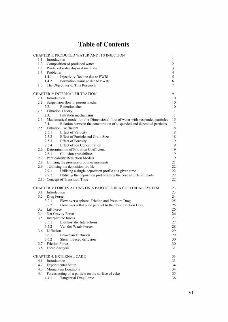
Table of Contents CHAPTER 1: PRODUCED WATER AND ITS INJECTION 1
1.1 Introduction 1 1.2 Composition of produced water 2 1.3 Produced water disposal methods 3 1.4 Problems 4
1.4.1 Injectivity Decline due to PWRI 5 1.4.2 Formation Damage due to PWRI 6
1.5 The Objectives of This Research 7 CHAPTER 2: INTERNAL FILTRATION 9
2.1 Introduction 10 2.2 Suspension flow in porous media 10
2.2.1 Retention sites 10 2.3 Filtration Theory 11
2.3.1 Filtration mechanisms 11 2.4 Mathematical model for one-Dimensional flow of water with suspended particles 15
2.4.1 Relation between the concntration of suspended and deposited particles 17 2.5 Filtration Coefficient 18
2.5.1 Effect of Velocity 18 2.5.2 Effect of Particle and Grain Size 18 2.5.3 Effect of Porosity 19 2.5.4 Effect of Ion Concentration 19
2.6 Determination of Filtration Coefficient 19 2.6.1 Collision probabilities 19
2.7 Permeability Reduction Models 19 2.8 Utilising the pressure drop measurements 21 2.9 . Utilising the deposition profile 22
2.9.1 Utilising a single deposition profile at a given time 22 2.9.2 Utilising the deposition profile along the core at different parts 22
2.10 Concept of Transition Time 22 CHAPTER 3: FORCES ACTING ON A PARTICLE IN A COLLOIDAL SYSTEM 23
3.1 Introduction 23 3.2 Drag Force 24
3.2.1 Flow over a sphere: Friction and Pressure Drag 25 3.2.2 Flow over a flat plate parallel to the flow: Friction Drag 25
3.3 Lift Force 26 3.4 Net Gravity Force 26 3.5 Interparticle forces 27
3.5.1 Electrostatic Interactions 27 3.5.2 Van der Waals Forces 28
3.6 Diffusion 29 3.6.1 Brownian Diffusion 29 3.6.2 Shear induced diffusion 30
3.7 Friction Force 30 3.8 Force Analysis 31
CHAPTER 4: EXTERNAL CAKE 33
4.1 Introduction 33 4.2 Experimental Setup 34 4.3 Momentum Equations 34 4.4 Forces acting on a particle on the surface of cake 35
4.4.1 Tangential Drag Force 36
VIII
4.4.2 Normal Drag Force 36 4.4.3 Electrostatic Forces 36 4.4.4 Frictional Force 36
4.5 Solving for the Force Balance Equality 36 4.6 Mass Balance Equations 37
4.6.1 Steady State Case 37 4.6.2 Transient Case with Erosion 38
CHAPTER 5: THE SETUP AND EXPERIMENTS 43
5.1 Introduction 43 5.2 Description of the set up 45
5.2.1 Injection Unit 45 5.2.2 Dynamic Filtration Unit (DFU) 46 5.2.3 Effluent Concentration Detection Unit (ECDU) 46
5.3 The Core (Porous Media) 47 5.4 Preparation of the core sample 48 5.5 Particle Properties 49
5.5.1 Hematite Particles 49 5.5.2 Latex Particles 49
5.6 Preparation of the Injected Suspension 49 5.7 Experiments 49
CHAPTER 6: INTERNAL DAMAGE RESULTS AND ANALYSIS 51
6.1 Introduction 51 6.2 Deposition Profile Obtaining Methods 51
6.2.1 Chemical Analysis 51 6.2.2 X-ray Tomography 52
6.3 Experiments 54 6.3.1 Static Experiment and Data Analysis 54 6.3.2 Dynamic Filtration Experiments 60
CHAPTER 7: EXTERNAL CAKE RESULTS AND ANALYSIS 65
7.1 Introduction 65 7.2 Simulation Results for Steady State case 66 7.3 Sensitivity Analysis 69
CHAPTER 8: CONCLUSIONS AND RECOMMENDATIONS 71
8.1 Conclusions 71 8.2 Recommendations 72
REFERENCES 75 NOMENCLATURE 78 Appendix A: ENVIRONMENTAL EFFECTS AND COMPOSITION OF PRODUCED WATER
83
Appendix B: DERIVATION OF ADVECTION-DIFFUSION EQUATION 87
B.1 Mass Balance Equation for C.V 87 B.2 Convection- Diffusion Equation 88
Appendix C: SOLUTION OF THE CONVECTION EQUATION WITH CONSTANT FILTRATION COEFFICIENT USING METHOD OF CHARACTERISTIC
89
C.1 Solution 89 C.2 Second method 90 C.3 Construction of the solution using Maple 91
IX
Appendix D: DERIVATION OF THE NAVIER STOKES EQUATION 95 D.1 Force balance 95 D.2 Infinite Plate Approximation 96 D.3 Equivalent Circular Tube Approximation 98 D.4 Comparison between the two approaches 98
Appendix E: DERIVATION OF EQUATION FOR THE EXTERNAL CAKE 99
Nomenclature 100 E.1 Force Balance 100
E.1.1 Tangential Drag Force 101 E.1.2 Normal Drag Force 103 E.1.3 Electrostatic Forces 103 E.1.4 Frictional Force 103
E.2 Solving for the Force Balance Inequality 103 E.3 Derivation of Equations at Steady State Condition 104 E.4 Derivation of Equations for Transient Case (No Erosion) 109 E.5 General Case: Considering both Deposition and Erosion 110 E.6 Mass Balance Equations for Suspension (With Erosion) 112
Appendix F: SATURATION PROCEDURE 115
F.1 Pre-Saturation Preparation of the Setup 115 F.2 Saturation Procedure 116 F.3 Deaeration of the set up 117
Appendix G: UNSUCCESSFUL STORIES WITH LATEX PARTICLES 121 Appendix H: CAN HEMATITE BE DETECTED USING CT SCANNER? 123 Appendix I: EXPERIMENTAL RESULTS: GRAPHS AND DATA 127
I.1 Experiment 1 127 I.2 Experiment 2 131 I.3 Experiment 3 134 I.4 Experiment 4 137 I.5 Experiment 6 140 I.6 Experiment 7 143 I.7 Breakthrough Curves 147 I.8 Permeability Decline Curves 148
Appendix J: DESCRETISATION OF THE EQUATIONS AND SENSITIVITY OF CAKE THICHNESS TO DIFFERENT PARAMETERS
151
J.1 Discretisation of Steady State Equations 151 J.2 Discretisation of Transient Equations 152 J.3 Sensitivity analysis 156
ACKNOWLEDEGMENT 159

X
1
CHAPTER 1
1 PRODUCED WATER AND ITS INJECTION
1.1 Introduction Most oil and gas reservoirs have a natural water layer called formation water beneath the
hydrocarbon layer. Also to achieve maximum oil recovery, additional water is usually injected into the reservoir, which may be associated with hydrocarbons in the production. In the case of some gas production, produced water can be condensed water. Thus, the liquid that comes out of reservoir is not just hydrocarbons, but is frequently accompanied by water. The liquid production is in the form of a mixture of free water, an oil/water emulsion and oil. Furthermore, as an oil field matures the amount of produced water increases. This is because, after some time, the formation waters out due to the water injection process. The water-oil ratio varies from reservoir to reservoir. It also varies with time for a particular reservoir. Worldwide 75% of the production is water, but in some places this percentage may increase to 98%. Table 1-1 shows the amount of produced water and oil in North Sea.
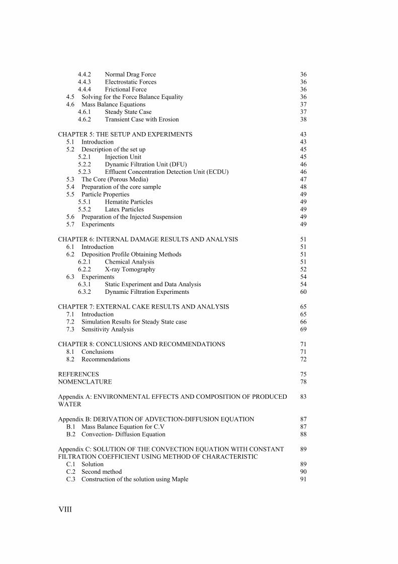
The production stream goes to a separation unit called the Free Water Knockout Vessel (FWKV). In this unit free water and loose solids are separated from oil. Produced water from this unit is stored in Water Tanks, while the remaining oil and oil-water emulsion are additionally treated. In Treater Vessels with the combination of heat and some chemicals (Emulsion Breakers or Demulsifiers) oil-water emulsions are broken down and clean oil, water and some solids are produced. Clean oil goes to storage or shipping and produced water is kept for disposal in Water Tanks. Depending on the residence time some of the solids may settle out of the water and residual oil in the water floats to the surface. This oil layer is skimmed off the top and recycled to recover this additional oil. In the fields with smaller
Produced Water Re-Injection
2
facilities in this stage water will go to be disposed, but in the larger facilities water faces an additional treatment in a Dissolved Air Floatation (DAF) to get cleaner water. After the DAF unit, the water is either sent through filters, which are usually sand and multimedia filters or through hydrocyclones to remove the remaining traces of oil and solids. After final filtration the water is ready to be disposed. Figure 1-1 shows a simple schematic of a separation unit.
Figure 1-1: Schematic of a simple separation unit. Worldwide 3 barrels out of 4 barrels of production is water and just one barrel is oil.
1.2 Composition of produced water Physical and chemical properties of the produced water mainly depend on geographical
location, geological formation and type of hydrocarbons of the field and may differ from one place to another. Since the produced water has been in contact with geological formations for millions of years, its composition is strongly field-dependent.
Produced water consists of a major part, water, and minor amounts of organic and inorganic constituents from the source geologic formation and the associated hydrocarbons. The composition of produced water may change through the production lifetime of the reservoir, because more water is injected to maintain the pressure of the reservoir. Produced water may also contain small amounts of chemicals that have been added in the treatment of water. These treatment chemicals could be listed as: Hydrate Inhibitors, Dehydrators, Scale Inhibitors, Corrosion Inhibitors, Bactericides, Emulsion Breakers, Coagulants, Flocculants, Defoamers, Paraffin inhibitors and solvents. In terms of salinity, most produced waters are more saline than sea water.
Table 1-1: Produced Water Discharges, North Sea
Year Number of installations
Water quantity (millions of tonnes) Oil levels (ppm) Oil quantity (tonnes)
1996 59 210 27 5,706 1997 64 234 25 5,764 1998 67 253 22 5,690 Canadian Association of Petroleum Product, Technical Report, August 2001
1.3 Produced water disposal methods Produced water is the largest single wastewater stream in oil and gas production. With the
increasing amount of produced water, handling of produced water has become one of the main issues in petroleum industry. Required facilities and equipment for treatment of the produced water are expensive. Therefore companies are trying to develop new technologies to minimize the production of water and consequently reduce the costs of water treatment
separator Productio
Wate
OiPRODUCTION OIL
WATER
1. Produced Water and Its Injection
3
methods and look for ways that with existing facilities can handle larger volumes of water. Produced water from onshore wells is recycled and reused.
There are different ways of disposing produced water. Some of the common methods are:
• Evaporation pits:
• Surface discharge/overboard disposal
• Deep aquifer injection
• Agricultural use (Irrigation of fruit trees or forage land…)
• Industrial use (Dust control, Vehicle washwater, power generation…)
• Desert flooding / livestock water pits
• Shallow water aquifer recharge
• Produced Water Re-Injection (PWRI)
It should be noted that the choice of produced water disposal methods is dependent on several factors, such as site location, regulatory acceptance, technical feasibility, cost and availability of infrastructure and equipment.
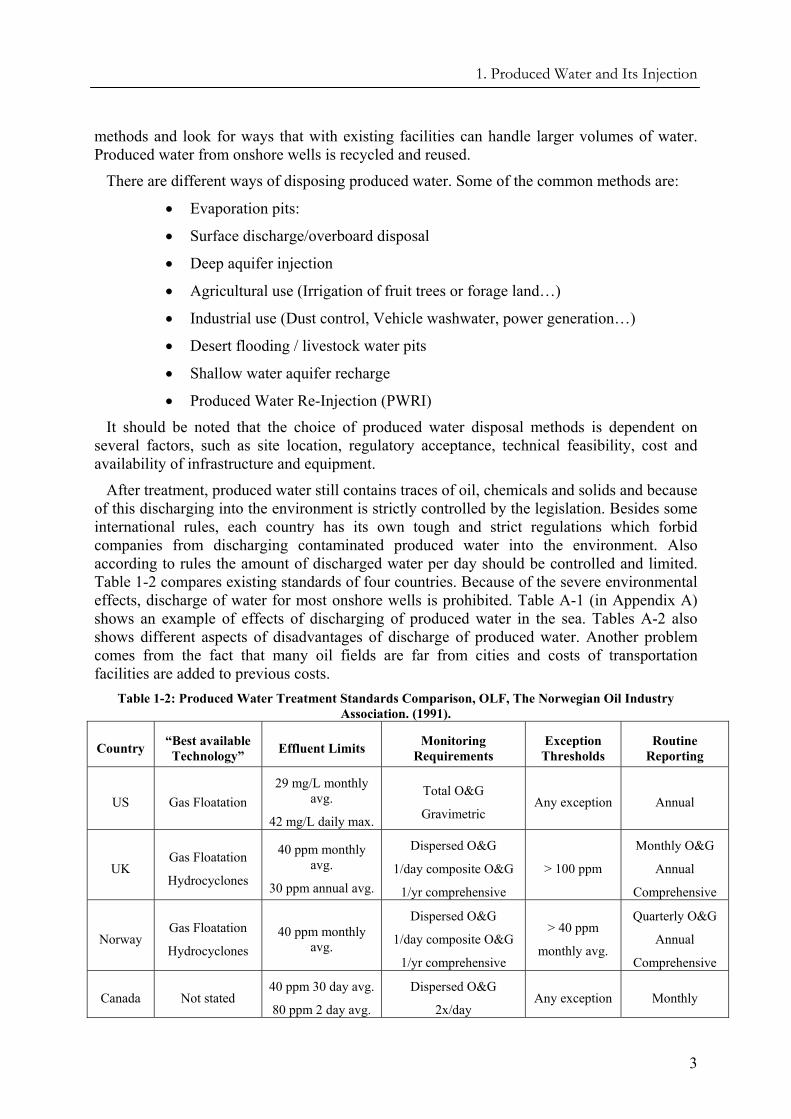
After treatment, produced water still contains traces of oil, chemicals and solids and because of this discharging into the environment is strictly controlled by the legislation. Besides some international rules, each country has its own tough and strict regulations which forbid companies from discharging contaminated produced water into the environment. Also according to rules the amount of discharged water per day should be controlled and limited. Table 1-2 compares existing standards of four countries. Because of the severe environmental effects, discharge of water for most onshore wells is prohibited. Table A-1 (in Appendix A) shows an example of effects of discharging of produced water in the sea. Tables A-2 also shows different aspects of disadvantages of discharge of produced water. Another problem comes from the fact that many oil fields are far from cities and costs of transportation facilities are added to previous costs.
Table 1-2: Produced Water Treatment Standards Comparison, OLF, The Norwegian Oil Industry Association. (1991).
Country “Best available Technology” Effluent Limits Monitoring
Requirements Exception
Thresholds Routine
Reporting
US Gas Floatation 29 mg/L monthly
avg.
42 mg/L daily max.
Total O&G
Gravimetric Any exception Annual
UK Gas Floatation
Hydrocyclones
40 ppm monthly avg.
30 ppm annual avg.
Dispersed O&G
1/day composite O&G
1/yr comprehensive
> 100 ppm
Monthly O&G
Annual
Comprehensive
Norway Gas Floatation
Hydrocyclones 40 ppm monthly
avg.
Dispersed O&G
1/day composite O&G
1/yr comprehensive
> 40 ppm
monthly avg.
Quarterly O&G
Annual
Comprehensive
Canada Not stated 40 ppm 30 day avg.
80 ppm 2 day avg.
Dispersed O&G
2x/day Any exception Monthly
Produced Water Re-Injection
4
The only potential alternative to surface discharge of produced water is underground injection. In underground injection of produced water some factors like availability of space or load capacity for added equipment required for injection, including additional tanks, water treatment equipment and injection pumps should be considered. The subsurface formation must be capable of receiving the injected water at rates equal to or greater than the production rate. This may require several wells. The subsurface formation must also have long term capacity to accept the produced water volumes that will be generated.
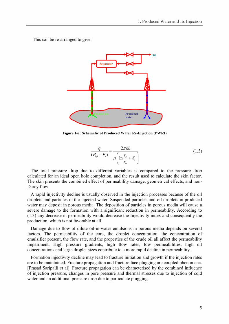
The pressure of a reservoir decreases with time leading to significant reduction in the production. Thus in order to produce more oil pressure should be maintained. There are different ways to enhance oil recovery; one of them is water injection. Therefore, one of the most economical and environmentally friendly methods of discarding the produced water is its re-injection into a suitable subsurface formation. Figure 1-2 shows the schematic of the produced water re-injection process. By re-injecting the produced water into the actual oil reservoir the other problem of pressure maintenance is also solved simultaneously. Thus, the produced water that would have been a waste product has been transformed to a money resource. In summary the benefits of produced water re-injection (PWRI) are:
• Disposal of produced water
• Pressure maintenance and displacing the crude oil in the reservoir
• Environmentally friendly
• Economic advantages
• Meets new regulations
1.4 Problems Produced water handling has become a major effort of all waterflood operations. With
increasing environmental regulations, more and more produced water is being re-injected. But like other operations, PWRI suffers some problems. The water that comes from the separators is definitely not pure water. It is comprised of water containing residual hydrocarbons, heavy metals, radionuclides, numerous inorganic species, suspended solids and chemicals used in treatment and hydrocarbon extraction. Presence of these contaminants will result in injectivity decline and formation damage.
1.4.1 Injectivity Decline due to PWRI The ease with which a fluid can be pumped into a well is measured as the ratio of the volume entering the formation during a period of time to the pressure differential between the well bore and the reservoir. The value of the ratio is called “Injectivity Index”.
2 t
skin
q SP kh
µπ
=∆
(1.1)
Here St is the total skin factor, q the injection flow rate and k the permeability of the reservoir. The expression can be combined with Darcy’s law to give:
ln( ) 2
et
inj e w
rq SP P kh r
µπ
⎛ ⎞= +⎜ ⎟− ⎝ ⎠
(1.2)
1. Produced Water and Its Injection
5
This can be re-arranged to give:
Figure 1-2: Schematic of Produced Water Re-Injection (PWRI)
2( )
lninj e et
w
q khP P r S
r
π
µ=
− ⎛ ⎞+⎜ ⎟
⎝ ⎠
(1.3)
The total pressure drop due to different variables is compared to the pressure drop calculated for an ideal open hole completion, and the result used to calculate the skin factor. The skin presents the combined effect of permeability damage, geometrical effects, and non-Darcy flow.
A rapid injectivity decline is usually observed in the injection processes because of the oil droplets and particles in the injected water. Suspended particles and oil droplets in produced water may deposit in porous media. The deposition of particles in porous media will cause a severe damage to the formation with a significant reduction in permeability. According to (1.3) any decrease in permeability would decrease the Injectivity index and consequently the production, which is not favorable at all.
Damage due to flow of dilute oil-in-water emulsions in porous media depends on several factors. The permeability of the core, the droplet concentration, the concentration of emulsifier present, the flow rate, and the properties of the crude oil all affect the permeability impairment. High pressure gradients, high flow rates, low permeabilities, high oil concentrations and large droplet sizes contribute to a more rapid decline in permeability.
Formation injectivity decline may lead to fracture initiation and growth if the injection rates are to be maintained. Fracture propagation and fracture face plugging are coupled phenomena. [Prasad Saripalli et al]. Fracture propagation can be characterised by the combined influence of injection pressure, changes in pore pressure and thermal stresses due to injection of cold water and an additional pressure drop due to particulate plugging.
Production Produced water
Separator
Oil
Produced Water Re-Injection
6
1.4.2 Formation Damage due to PWRI Subsurface injection of produced water generally leads to damage of the formation into
which the water is injected. Formation Damage can be defined as a reduction in permeability of the formation. Formation damage leads to loss of production and/or injectivity and consequently loss of money. Several parameters play role in the process of formation damage. The rate and extent of the damage strongly depends on the properties of the porous medium in which the produced water is injected and the characteristics of the injected water itself. In porous media size and distribution of pores and throats and connectivity of pores are important parameters. Concentration and size distribution of particles and also injection rate of the produced water are the parameters which determine the damage to the formation. The problem of formation damage due to PWRI can be decomposed into separate distinct problems. These include internal filtration, external filter cake build-up and the associated permeability reduction (formation damage).
Depending on the details of the case under investigation (e.g. contaminant size with respect to porous medium pore throat size, surface charge, injection rate, etc.) one of the following scenarios may be applicable:
• Pure internal filtration of the contaminants
• Pure external filter cake build-up
• Initial internal filtration followed by external filter cake build-up after a certain transition time *t
• Initial internal filtration followed by simultaneous internal filtration and external cake build-up after a certain transition time.
It is important to know the performance of injection wells as a function of the amount of the suspended particles in the water. Some important decisions should be made in order to quantify the damage. This, being a major issue, attracted researches and many investigations have been conducted. Barkman and Davidson [Barkman et al. (1972)] were among the first ones who investigated the injectivity decline for PWRI. They defined the injectivity half time, which is the time required for the initial injection rate to decrease to 50% of this rate. The formation damage is caused by four mechanisms: welbore narrowing, invasion, perforation plugging, and welbore fill-up. For each mechanism they introduce an equation to predict the half-life of an injection well based on the water quality ratio. Water quality ratio (WQR) is the ratio of the concentration of solids to the permeability of the filter cake formed by those solids. The WQR can be measured in the laboratory with constant pressure drop test using cores or membrane filters. As cake filtration proceeds, the filtration volume V will grow linearly with t . The slope of the V- t plot may be used to calculate the WQR. Barkman and Davidson could apply their equations just for constant pressure conditions, whereas real injectors are rate-controlled. Hofsaess and Kleintz (2003) introduce a revised equation for the WQR after Barkman and Davidson. They introduced the half-volume concept and presenting the injectivity decline in terms of accumulated injection volume, they overcome the problem of using constant pressure. The latest proposed models [M.M. Sharma (1994), D.Marchesin, P.Bedrikovetsky (2002)] about the injectivity decline are mainly based on classical deep bed filtration in which they try to find a filtration coefficient and damage coefficient which conform with the obtained data from the laboratory experiments. This theory will be explained more in chapter 2.
1. Produced Water and Its Injection
7
1.5 The Objectives of This Research Due to the importance of the environmental issues and the huge amount of produced water,
the subsurface injection of produced water has earned a lot of attention. Although it is known that the re-injection of the produced water would damage the formation and result in the reduction of the production, the extent and mechanism of the damage is still unclear. The objective of this study is to carry out laboratory experiments in order to investigate and predict the damage. This research is done both on internal filtration and external cake build up. For the internal filtration results the classical deep bed filtration theory will be applied. For the external cake build up a new model which is developed by the PWRI group is presented.

Produced Water Re-Injection
8
9
CHAPTER 2
2 INTERNAL FILTRATION
2.1 Introduction
The problem of formation damage is split into two separate parts which includes internal filtration and external cake build-up. In this chapter we will discuss the theories and proposed models of internal damage resulting from produced water re-injection.
In this chapter, first flow of the suspension in a porous medium is explained. Then the retention sites and filtration mechanism are introduced. The filtration theory and its mathematical modelling are also given in this chapter. In the following section, the filtration coefficient and effect of the different parameters will be explained. Finally, the permeability reduction models will be discussed. The permeability reduction model tries to model the effect of particle deposition on flow properties such as permeability. Consequently, different measurement techniques are discussed and description is given to how they are used to obtain the unknown parameters in the filtration theory.
2.2 Suspension flow in porous media Porous media (rocks, soils, catalyst pellets, packed beds…) and particulate systems
(suspensions, colloids, emulsions, bacteria…) are present in most engineering practices. Consequently a lot of investigations have been done in order to understand the mechanisms of the transport of the particulate matters through a porous medium. However, due to the complexity of the transport phenomena this issue is not fully understood.
Produced Water Re-Injection
10
Throughout this review colloidal materials suspended in water are referred to as particles. A porous medium is a fixed bed of granular materials with pores through which fluid can flow. Apparently, when a suspension flows through a porous medium, particles are brought in contact with retention sites. In this case there are two possibilities for particles: either they are deposited or they are carried away by the stream. Separation of particles can change the fluid properties as well as the permeability of the medium. The reduction in permeability value can be simply determined by applying Darcy’s law for different conditions.
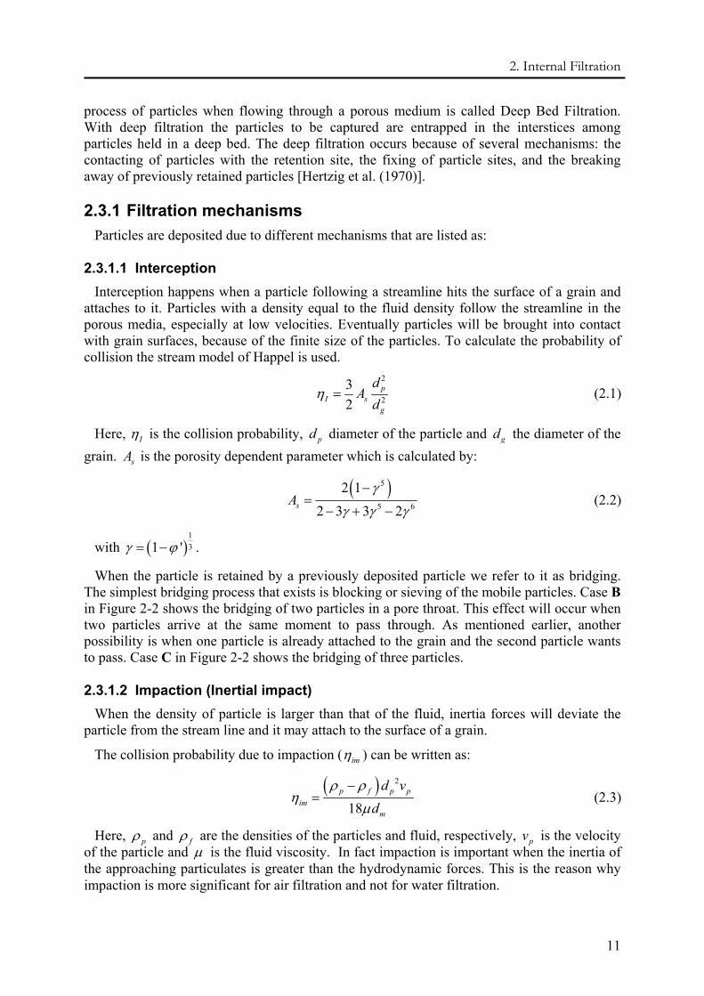
2.2.1 Retention sites Each sand grain can collect a number of particles in the porous medium. Therefore the
deposition surface is called the collector. There are various sites that can retain a particle when transported through a porous medium.
2.2.1.1 Surface sites In this case, a particle stops when it reaches a grain surface, and is deposited on the surface
of the grain. This happens when the particle is too large to penetrate into the medium.
2.2.1.2 Crevice sites Sorting and ordering of the grains may result in forming convex surfaces. Thus, some
particles will get stuck at the convex surfaces.
2.2.1.3 Constriction sites When the diameter of a particle is larger than that of a pore, particle will stop and get
deposited.
2.2.1.4 Cavern sites A particle may find some sheltered area in its path and stay there. These sheltered areas are
small pockets formed by several grains. In these shelters the particles are protected from the flow stream.
(a) (b) (d)(c)(a) (b) (d)(c)
Figure 2-1: Different retention sites: (a) surface site, (b) crevice site, (c) constriction site, (d) cavern site
2.3 Filtration Theory When fluid containing particles reaches a porous medium, the liquid and the solid phases in
the suspension can be separated, either by depositing in the pore or accumulating in front of the surface. This is similar to what happens in the filtration process. Then, the retention
2. Internal Filtration
11
process of particles when flowing through a porous medium is called Deep Bed Filtration. With deep filtration the particles to be captured are entrapped in the interstices among particles held in a deep bed. The deep filtration occurs because of several mechanisms: the contacting of particles with the retention site, the fixing of particle sites, and the breaking away of previously retained particles [Hertzig et al. (1970)].
2.3.1 Filtration mechanisms Particles are deposited due to different mechanisms that are listed as:
2.3.1.1 Interception Interception happens when a particle following a streamline hits the surface of a grain and
attaches to it. Particles with a density equal to the fluid density follow the streamline in the porous media, especially at low velocities. Eventually particles will be brought into contact with grain surfaces, because of the finite size of the particles. To calculate the probability of collision the stream model of Happel is used.
2
2
32
pI s
g
dA
dη = (2.1)
Here, Iη is the collision probability, pd diameter of the particle and gd the diameter of the grain. sA is the porosity dependent parameter which is calculated by:
( )5
5 6
2 1
2 3 3 2sAγ
γ γ γ
−=
− + − (2.2)
with ( )131 'γ ϕ= − .
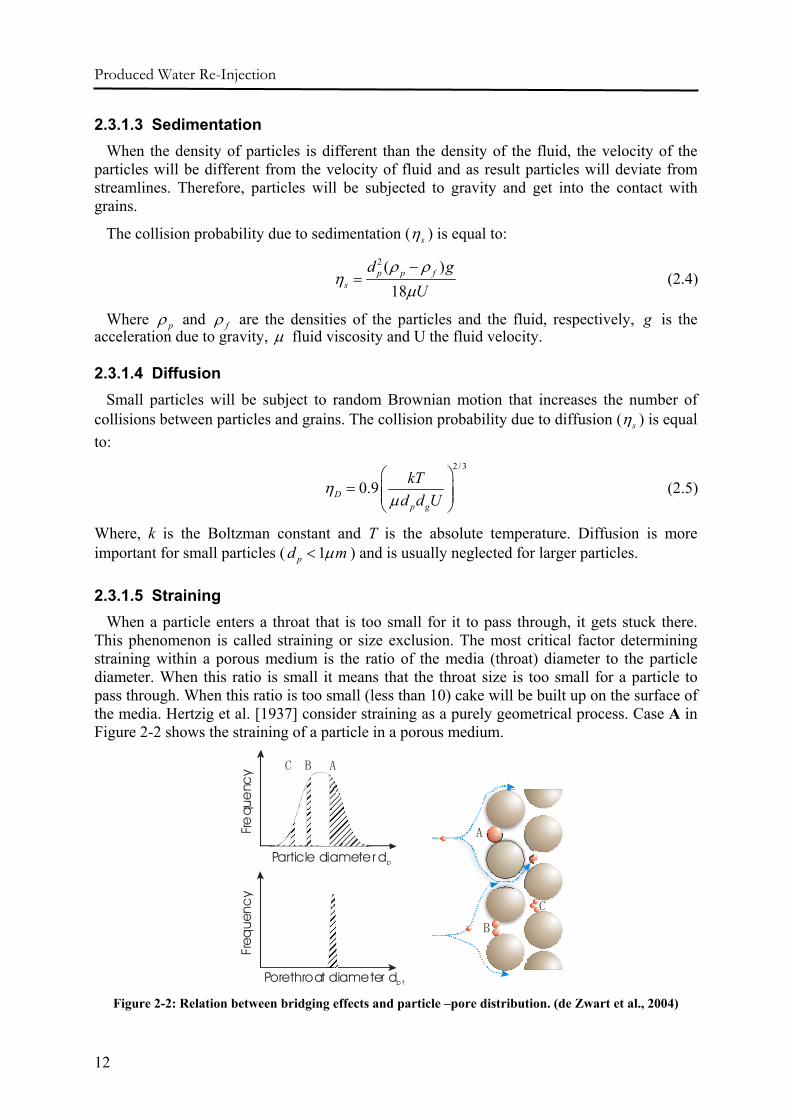
When the particle is retained by a previously deposited particle we refer to it as bridging. The simplest bridging process that exists is blocking or sieving of the mobile particles. Case B in Figure 2-2 shows the bridging of two particles in a pore throat. This effect will occur when two particles arrive at the same moment to pass through. As mentioned earlier, another possibility is when one particle is already attached to the grain and the second particle wants to pass. Case C in Figure 2-2 shows the bridging of three particles.
2.3.1.2 Impaction (Inertial impact) When the density of particle is larger than that of the fluid, inertia forces will deviate the
particle from the stream line and it may attach to the surface of a grain.
The collision probability due to impaction ( imη ) can be written as:
( ) 2
18p f p p
imm
d vd
ρ ρη
µ−
= (2.3)
Here, pρ and fρ are the densities of the particles and fluid, respectively, pv is the velocity of the particle and µ is the fluid viscosity. In fact impaction is important when the inertia of the approaching particulates is greater than the hydrodynamic forces. This is the reason why impaction is more significant for air filtration and not for water filtration.
Produced Water Re-Injection
12
2.3.1.3 Sedimentation When the density of particles is different than the density of the fluid, the velocity of the
particles will be different from the velocity of fluid and as result particles will deviate from streamlines. Therefore, particles will be subjected to gravity and get into the contact with grains.
The collision probability due to sedimentation ( sη ) is equal to:
2 ( )
18p p f
s
d gU
ρ ρη
µ−
= (2.4)
Where pρ and fρ are the densities of the particles and the fluid, respectively, g is the acceleration due to gravity, µ fluid viscosity and U the fluid velocity.
2.3.1.4 Diffusion Small particles will be subject to random Brownian motion that increases the number of
collisions between particles and grains. The collision probability due to diffusion ( sη ) is equal to:
2 /3
0.9Dp g
kTd d U
ηµ
⎛ ⎞= ⎜ ⎟⎜ ⎟
⎝ ⎠ (2.5)
Where, k is the Boltzman constant and T is the absolute temperature. Diffusion is more important for small particles ( 1pd mµ< ) and is usually neglected for larger particles.
2.3.1.5 Straining When a particle enters a throat that is too small for it to pass through, it gets stuck there.
This phenomenon is called straining or size exclusion. The most critical factor determining straining within a porous medium is the ratio of the media (throat) diameter to the particle diameter. When this ratio is small it means that the throat size is too small for a particle to pass through. When this ratio is too small (less than 10) cake will be built up on the surface of the media. Hertzig et al. [1937] consider straining as a purely geometrical process. Case A in Figure 2-2 shows the straining of a particle in a porous medium.
Porethroat diameter dp t
Freq
uenc
y
A
B
C
Particle diameter dp
Fre
que
ncy ABC
Figure 2-2: Relation between bridging effects and particle –pore distribution. (de Zwart et al., 2004)
2. Internal Filtration
13
2.3.1.6 Surface forces Van der Waals attraction forces and double layer repulsion forces are also significant for the capture of the particles. (For more details see Chapter 4)
The above mentioned mechanisms will play role in the deposition process of the particle in contact with the grain surface. The dominance of the force is depending on filtration medium properties, particle properties and flow. Details of surface forces (van der Waals attraction forces and double layer repulsive forces) will determine whether a particle will stick to the grain or not. In other words, if the sum of the hydrodynamic and electrostatic forces is attractive, a particle will be retained and if the sum is repulsive particles will not adhere to the grain.
Rajagopalan proposed an equation to calculate the collision probabilities in which the collision probability due to electrostatic forces is calculated by:
( )
1/8 13/8
1/8 15/8
49
pE s
p g
dAAv d
ηπµ ϕ
⎛ ⎞⎛ ⎞ ⎜ ⎟= ⎜ ⎟ ⎜ ⎟⎝ ⎠ ⎝ ⎠ (2.6)
Where, A is the Hamaker constant ( )2010 J− .
The total collision probability due to diffusion, interception, impaction, surface forces and sedimentation is calculated by:
ImD I S Eη η η η η η= + + + + (2.7)
The total collision probability can be used to estimate the filtration coefficient, which will be explained later.
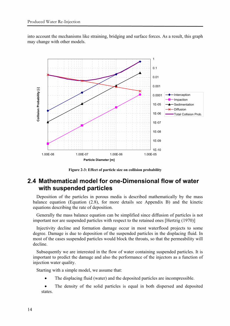
Table 2-1: Input Data for Figure 2-3
Porosity 0.23 [-] Diameter of Grains 100 [ mµ ]
Density of Particles 5400 [ 3/kg m ]
Density of Fluid 1000 [ 3/kg m ] Viscosity of Fluid 0.001 [Pa.sec]
Velocity 0.002 [m/sec]
Depending on the size and shape of the particles one of the above mentioned mechanisms will prevail. For example for very small particles surface and diffusion forces become most important while for larger particles these mechanism become less important. Figure 2-3 shows the effect of size of the particles and media on the total collision probability and the dominant mechanisms in different sizes of particles. To obtain this graph values in Table 2-1 were used, which are characteristic of the core samples, the fluids and the velocities we used in our experiments. Figure 2-3 indicates that in our experiments (1 10pd mµ< < ), the more dominant mechanism is interception. Also it can be seen that for the range of velocities we use, impaction is negligible according to the model we use. Since the effect of diffusion is an order of magnitude smaller than that of interception we neglect the effect of diffusion in our modelling. We have to notice that the model we have used to plot this graph does not take
Produced Water Re-Injection
14
into account the mechanisms like straining, bridging and surface forces. As a result, this graph may change with other models.
1E-10
1E-09
1E-08
1E-07
1E-06
1E-05
0.0001
0.001
0.01
0.1
1
1.00E-08 1.00E-07 1.00E-06 1.00E-05
Particle Diameter [m]
Col
lisio
n Pr
obab
ility
[-]
InterceptionImpactionSedimentationDiffusionTotal Collision Prob.
Figure 2-3: Effect of particle size on collision probability
2.4 Mathematical model for one-Dimensional flow of water with suspended particles
Deposition of the particles in porous media is described mathematically by the mass balance equation (Equation (2.8), for more details see Appendix B) and the kinetic equations describing the rate of deposition.
Generally the mass balance equation can be simplified since diffusion of particles is not important nor are suspended particles with respect to the retained ones [Hertzig (1970)]
Injectivity decline and formation damage occur in most waterflood projects to some degree. Damage is due to deposition of the suspended particles in the displacing fluid. In most of the cases suspended particles would block the throats, so that the permeability will decline.
Subsequently we are interested in the flow of water containing suspended particles. It is important to predict the damage and also the performance of the injectors as a function of injection water quality.
Starting with a simple model, we assume that:
• The displacing fluid (water) and the deposited particles are incompressible.
• The density of the solid particles is equal in both dispersed and deposited states.
2. Internal Filtration
15
• The velocity of the fluid along the core is constant. Also we assume a constant velocity with time. Therefore, the conservation of the total flux is:
divU = 0
• The volume of the entrapped particles is negligible compared to the effective porosity. (σ ϕ<< )
• The kinetics of the particles is linear.
• The dependency of the viscosity on concentration is negligible.
• Diffusive and dispersive effects are negligible.
For such a problem, the mass conservation equation for the retained and deposited particles in linear flow of an incompressible fluid can be written as:
( ) 0cc Ut xϕ σ∂ ∂
+ + =∂ ∂
(2.8)
Here ϕ is the effective porosity, ( , )c x t and ( , )x tσ are the volumetric concentrations of the suspended and deposited particles respectively. c can have values between 0 and 1, whereas the quantity σ has values between 0 andϕ . ( 0 1,0c σ ϕ≤ ≤ ≤ ≤ ). (2.8) basically states that net increase of the particles in the system is equal to the upstream entering particles minus the downstream exiting particles minus the deposited particles.
In this model we assume that permeability reduction is only due to the deposition of particles and that permeability is a decreasing function of the deposited concentration.
Darcy’s law relates superficial velocity to pressure:
0 ( )k k PUx
σµ
∂= −
∂ (2.9)
Here 0k is the absolute permeability, ( )k σ is the relative permeability, when expressed as a function of σ , it is also called “Formation Damage Function”. It can be normalized so that:
(0) 1k =
The rate of deposition is proportional to the concentration of suspended particles and fluid velocity:
( ) U ctσ λ σ∂=
∂ (2.10)
The constant of proportionality ( )λ σ is the “Filtration Coefficient” function. (2.10) is only valid if σ ϕ otherwise ϕ would change with deposition and problem would be more complicated.
The filtration coefficientλ is a function of deposited particles σ and fluid velocity. In our model we assume that the velocity is constant, thus automatically we neglect the effect of velocity and we write ( )λ σ instead of ( , )Uλ σ . However, it is important to mention that for radial flow near the borehole the velocities are very large and the velocity effect becomes important.
We introduce dimensionless length, time, scaled concentration C and the filtration coefficientλ as:
Produced Water Re-Injection
16
1
0
0( ) ( )
X xLU
T tL
cC
c
Sc
S L
ϕ
σ
ϕ
λ σ
=
=
=
=
Λ =
⎧⎪⎪⎪⎪⎪⎪⎨⎪⎪⎪⎪⎪⎪⎩
(2.11)
Then equations (2.8) and (2.10) become:
C C ST X T∂ ∂ ∂
+ = −∂ ∂ ∂
(2.12)
( )S S CT∂
= Λ∂
(2.13)
Combining (2.12) and (2.13) yields:
( ) 0C C S CT X∂ ∂
+ + Λ =∂ ∂
(2.14)
As can be seen to solve (2.14) we need to know the equation for filtration coefficient, λ . For example assuming a constant value forλ , the concentration profile can be obtained by:
0 XC e−Λ= (2.15)
[For more details see appendix C]. Marchesin et al. [2002] have solved (2.14) with taking different functions for ( )SΛ .
2.4.1 Relation between Concentration of Suspended and Deposited Particles
Putting (2.15) into (2.13) and solving the obtained equation will give the solution for deposition which is:
( )0 0( ) expT X Xσ = − Λ −Λ (2.16)
This solution is valid when T X≥ .
Hertzig et al. [1970] proved the following relation between σ and c and their initial values:
( )( )
( )( )
, ,0, 0,
c X T X Tc T T
σσ
= (2.17)
(2.17) applies when c and σ are taken at the same depth X , and 0, , c c σ and 0σ are taken at the same T. Hertzig et al. [1970] derived the following equation for the clogging front velocity:
2. Internal Filtration
17
FcTV U
X
σ
σ σ
∂∂= − =
∂∂
(2.18)
The existence of such a constant clogging front can be only seen in the plot of σ against x . Since /c x∂ ∂ depends on both c and σ this feature can be seen from the plot of c against x only if the concentration at the inlet of the core is assumed constant.
2.5 Filtration Coefficient The basic filtration equation (2.10) was proposed by Iwasaki [1937]. This equation basically
indicates that the rate of deposition is a function of the concentration and velocity of the suspension with the filtration coefficient as proportionality constant.
Equation (2.10) is sometimes called the “Kinetic Equation”. The filtration coefficient λ is a function of several parameters and has the dimension of 1m− . According to literature filtration coefficient is mainly dependent on the number of previously deposited particles, concentration of the suspension, velocity, size of the particles and size of the grains.
( , , , , ,...)p gc u d dλ λ σ= (2.19)
For the dilute suspensions the dependency on concentration is usually neglected in order to get a linear relationship between σ and c .
Hertzig et al. [1970], proposed different filtration coefficients for the different mentioned mechanisms. Generally, λ , can be related to superficial velocity and size of particles and grains as:
p
g
ud
d
α
β
γ
λ
−
−
⎧⎪⎪∝ ⎨⎪⎪⎩
(2.20)
2.5.1 Effect of Velocity As mentioned before for large particles, size exclusion or straining is the main mechanism
of deposition. When straining is the case or at least for the viscous flow regime, the filtration coefficient is not a function of velocity, leading to 0α = . When 1α = , the retention rate,
tσ∂∂
is independent of velocity. Fitzpatrick and Spielman [1973] did various experiments with
different particle sizes. They found out that α increases with increase in size of particles and its value is mostly between zero and two. Nevertheless, larger values for α have been reported (Ison et al. [1969]). In conclusion the dominant filtration mechanism determines the effect of velocity in the value of filtration coefficient. Moreover, Darcy’s velocity definition
uvϕ
⎛ ⎞=⎜ ⎟
⎝ ⎠ underestimates the interstitial velocity, because it does not take into account the
tortuosity and dead end porosity. Thus, it has been a big discussion whether Darcy’s velocity should be used or not (Rochon et al [1996]). When the effect of porosity on λ is considered separately, Darcy’s velocity can be used (Wennberg et al. [1997]).
Produced Water Re-Injection
18
2.5.2 Effect of Particle and Grain Size For small particles ( 1pd mµ< ) diffusion might be the main mechanism of the particle
transport through the porous medium. This will result in negative values for β in (2.20). For slightly larger particles β is positive. This means that the larger the size of the injected particle, the larger the value of the filtration coefficient. Negative and positive values mean the existence of a minimum value for β . This minimum can be determined experimentally (Fitzpatrick and Spielman [1973]). Also experiments show a value of between 0-2. The average value is about 0.9.
2.5.3 Effect of Porosity Higher porosity values will result in lower values for the filtration coefficient, because in
high porous rocks the available space for particles to be captured is higher. Fitzpatrick and Spielman [1973] did experiments at two different porosity values, 0.38 and 0.41. They found out that for latter case the values of the filtration coefficient were 30% lower than for the other case under all conditions.
2.5.4 Effect of Ion Concentration Experiments show that at electrolyte concentrations below 10-3 M, the filtration coefficient
starts to drop rapidly, because with increasing concentration the zeta potential ξ increases. A higher zeta potential means higher double layer repulsion forces. Therefore, higher concentrations make a barrier for the depositing of the particles.
2.6 Determination of Filtration Coefficient The filtration coefficient is a key parameter in the modeling of the water injection and, in
general, in formation damage problems. In order to solve the governing partial differential equation (2.14) we need to find a value or a function for λ . In this section different methods for finding λ are explained.
2.6.1 Collision probabilities Using (2.7) one can determine the total collision probability due to different filtration
mechanisms and calculate the filtration coefficient by:
( )132 c
gdϕ
λ α η′−
= (2.21)
Where cα is clean-bed collision efficiency. η can be calculated using any of the available models and cα is determined from experimental data. Putting (2.21) into (2.15) yields:
( )
0
13exp2 c
g
c Lc d
ϕα η
⎛ ⎞−= −⎜ ⎟⎜ ⎟
⎝ ⎠ (2.22)
Although this method is acceptable to fit the experimental data (Jiamhong et al. [2001]) it does not consider some mechanisms like straining. Nevertheless, it can be used to guess the initial value of the filtration coefficient.
2. Internal Filtration
19
2.7 Permeability Reduction Models Due to deposition the porous medium will change during filtration. This effect is
incorporated in the filtration function ( )F σ defined as: 0 ( )Fλ λ σ= , which defines the dependency of the filtration coefficient on the initial coefficient and deposition of the particles. Also for the filtration function a variety of empirical relations are found, based on different stages during filtration (filter ripening, re-entrainment or blocking). In Hertzig et al. [1970] a list of expressions of ( )F σ is given. The most general form is proposed by Ives [1970]:
00 0
1 1 1y z x
M
βσ σ σλ λφ φ σ
⎛ ⎞ ⎛ ⎞ ⎛ ⎞= + − −⎜ ⎟ ⎜ ⎟ ⎜ ⎟
⎝ ⎠⎝ ⎠ ⎝ ⎠ (2.23)
where , ,x yβ and z are empirical parameters and Mσ is the maximum value of σ for which λ drops to zero.
The extent of damage depends on the amount of deposited particles. Therefore, the reduction in permeability is linked to σ . Deposition of particles in the pores and throats of the medium will decrease the permeability. Since in the experiments one of the measured parameters is the pressure drop along the core, it is necessary to have the relationship between the permeability and the deposition concentration. To that end, the Kozeny-Carman equation is used:
( )22
0 3
16 6
g
d Uidx g d
ϕµϕ
⎛ ⎞−Φ= − = ⎜ ⎟⎜ ⎟
⎝ ⎠ (2.24)
Φ is the hydraulic head and 0i is the clean bed gradient. Combining Darcy’s law and (2.24) gives:
( )
2 3
2216 1ggd
K ϕµ ϕ
=−
(2.25)
K is the hydraulic conductivity which is related to medium permeability by:
.k gKµ
= (2.26)
Combining (2.25) and (2.26) leads to:
( )
2 3
2216 1gd
k ϕϕ
=−
(2.27)
(2.27) indicates that the permeability is only a function of the medium parameters. Nevertheless, deposition of the particles in the porous media increases the medium surface area to volume ratio and decreases the porosity. In literature there are some proposed models for increased head loss caused by deposited particles. Many of them are in the form of:
( )0
11 n
iRiσ
ασ= =
− (2.28)
Produced Water Re-Injection
20
where Rσ is the resistance due to deposition. α and n are positive parameters (McDowell-Boyer et al. [1986]. Using a power series (2.28) becomes:
( ) 2 211 ...
2n n
R nσ ασ α σ⎛ ⎞+
= + + +⎜ ⎟⎝ ⎠
(2.29)
By introducing nβ as formation damage factor a permeability reduction model can be written as:
21 2
1 11 ...
kRσσ β σ β σ
= =+ + +
(2.30)
2.8 Utilising the pressure drop measurements Impedance j is the inverse of the injectivity index.
PjU∆
= (2.31)
The non-dimensional form of impedance is:
1
0
0
PPJU U
−⎡ ⎤∆∆⎡ ⎤= ⎢ ⎥⎢ ⎥⎣ ⎦ ⎣ ⎦
(2.32)
where 0
0
PU∆ is the initial impedance of the system prior to injection of produced water.
The 3-point pressure method (Bedrikovetsky et al. [2001]) utilises Darcy’s law (2.33) and a linear resistance relationship for the resistance (2.34).
0 ( )k k PUx
σµ
∂= −
∂ (2.33)
1 1Rkσσ
βσ= = + (2.34)
Using these equations Bedrikovetsky et al. [2001] developed a model to calculate the filtration coefficient using pressure data at 3 points and the following equations:
( )( )01 Where 1 expJ mT m β= + = − Λ (2.35)
( )( )01 Where 1 expi i i iJ m T mω β ω= + = − Λ (2.36)
where i
i
TTω ω= , i
ixωL
= and T is the number of pore volumes injected.
As can be seen from (2.35) and (2.36) if we plot J vs. T , its slope will present the value of m and im . With these values and having the equation of Rσ , filtration coefficient could be calculated.
Although the linear relationship (2.34) is widely accepted, Al-Abduwani et al. [2004a] introduced quadratic relationship to calculate the filtration coefficient.
2. Internal Filtration
21
2.9 . Utilising the deposition profile
The deposition profile can be utilised in quantifying the filtration coefficient in two different ways:
2.9.1 Utilising a single deposition profile at a given time
In order to obtain the deposition profile Al-Abduwani et al. [2003] used a method called post-mortem analysis. This analysis gives an average value per segment iS< > . Therefore, the cumulative deposition iM in a given segment i can be obtained by:
( )1i i i iM S X X −=< > − (2.37)
or:
( )1
i
i
X
iX
M S X dX−
= ∫ (2.38)
Thus using ( )0 0expS T X= Λ −Λ we can write:
1i iX XiM y yT
−+ = (2.39)
where ( )0expy= −Λ . (2.39) can be solved for each segment separately or with putting Xi=0 and Xi=1, it can be used to calculate the cumulative deposition over the entire core.
2.9.2 Utilising the deposition profile along the core at different parts
To use this method we have to know the concentration and deposition profile at the same position at different times. Such information can be obtained if we assume that the average concentration in the last segment is what we measure in the effluent. The deposition profile can be obtained by non-invasive techniques such as CT-scanner monitoring (Al-Abduwani et al. [2004b]). The invasive way is to run multiple experiments with the same parameters and end them in different times. Then (2.13) becomes:
2 10 1,2
2 1
S S CT T
− =Λ−
(2.40)
from which the filtration coefficient can be calculated. This technique is a differential technique and suffers instability and magnificence of measurement errors.
2.10 Concept of Transition Time Experimental results show that when we start to inject, particles mostly deposit at inlet and
near inlet face, consequently pores will become filled with particles and after that external cake starts to build up. The time that this happens is called transition time. Transition occurs when porosity reaches critical porosity. Pang [1996] gave the following formula to calculate
Produced Water Re-Injection
22
the transition time:
*
*
0
1( )
nn
n g
dtC va nη
= ∫ (2.41)
where, n is the number of particles attached to one grain, n* the number of particles attached to one grain when 1η = , ga is the cross-sectional area of a grain, nC the number concentration of particle per unit liquid volume. To calculate ( )nη Pang determined the function from Stokesian dynamics simulation and found out that: 0 b nη η ′= + and therefore:
*
00
1 1ln( )
nndn bη η
=′∫ (2.42)
Pang and Sharma [1997] modified this concept. They choose to operate in terms of filtration coefficient rather than the collection efficiency. The concept of transition time is just an approximation and can never be exactly true.
23
CHAPTER 3
3 FORCES ACTING ON A PARTICLE IN A COLLOIDAL SYSTEM
3.1 Introduction Various forces act on a particle in a colloidal system. Particles are in a continuous motion
under the influence of these forces until they get deposited or go out of the system. These forces are:
• Drag forces • Lift forces • Net Gravity force • Brownian force • Screened electrostatic and steric repulsions • Van der Waals attractions • Friction Force
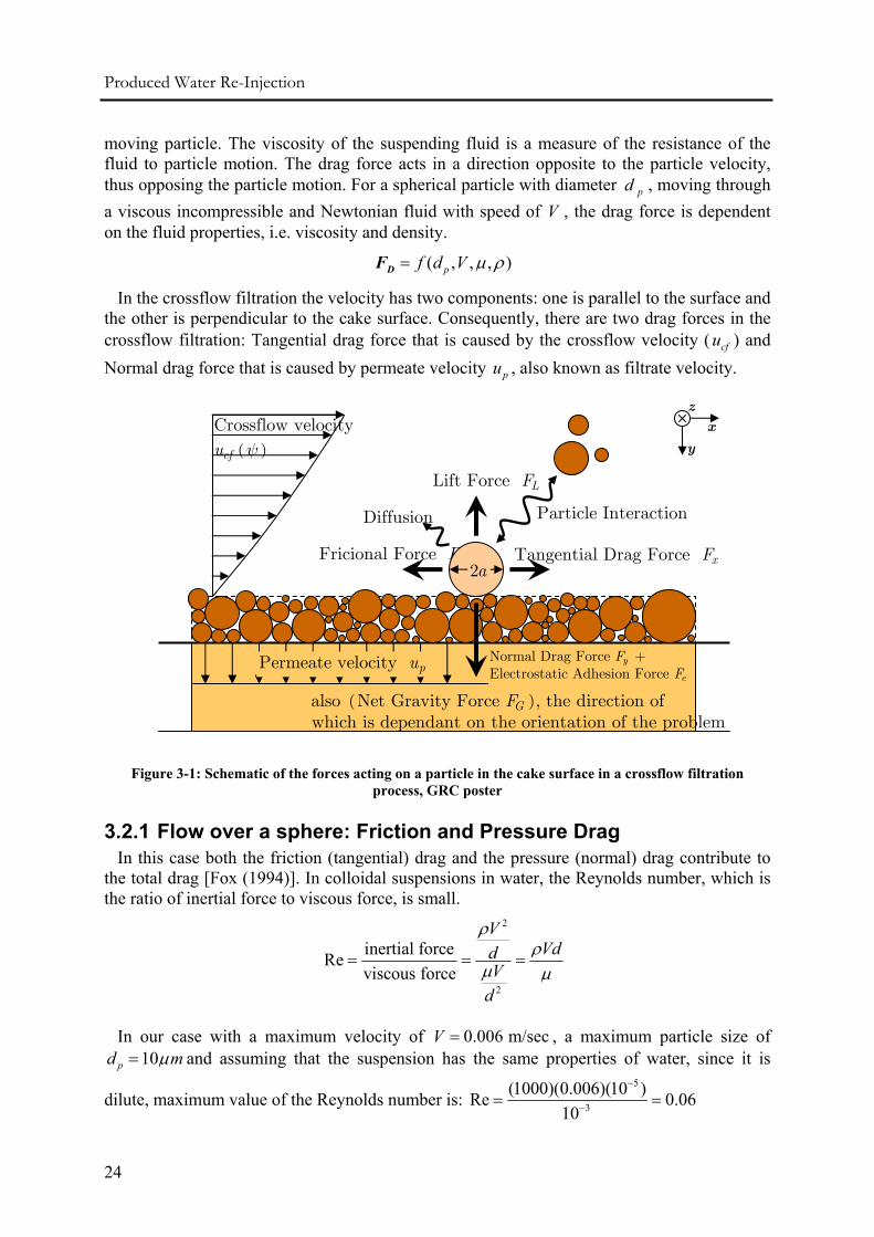
To understand the problem better and to be able to model the problem, origin and nature of these forces should be known and in order to simplify the problem some assumptions should be made. Figure 3-1 shows a particle on the cake surface with various forces acting on it. It should be noted that in this chapter we will consider both static (dead end) and dynamic (crossflow) filtration.
3.2 Drag Force Drag is the component of the force acting on a body parallel to the opposite direction to
motion. In colloidal systems drag forces arise due to the resistance of surrounding fluid to the motion of particles. The resistance is caused by the viscous shear of the fluid flowing over the particles and by the pressure difference between the upstream and downstream sides of the
Produced Water Re-Injection
24
moving particle. The viscosity of the suspending fluid is a measure of the resistance of the fluid to particle motion. The drag force acts in a direction opposite to the particle velocity, thus opposing the particle motion. For a spherical particle with diameter pd , moving through a viscous incompressible and Newtonian fluid with speed of V , the drag force is dependent on the fluid properties, i.e. viscosity and density.
( , , , )pf d V µ ρ=DF
In the crossflow filtration the velocity has two components: one is parallel to the surface and the other is perpendicular to the cake surface. Consequently, there are two drag forces in the crossflow filtration: Tangential drag force that is caused by the crossflow velocity ( cfu ) and Normal drag force that is caused by permeate velocity pu , also known as filtrate velocity.
Figure 3-1: Schematic of the forces acting on a particle in the cake surface in a crossflow filtration process, GRC poster
3.2.1 Flow over a sphere: Friction and Pressure Drag In this case both the friction (tangential) drag and the pressure (normal) drag contribute to
the total drag [Fox (1994)]. In colloidal suspensions in water, the Reynolds number, which is the ratio of inertial force to viscous force, is small.
2
2
inertial forceReviscous force
VVdd
Vd
ρρ
µ µ= = =
In our case with a maximum velocity of 0.006 m/secV = , a maximum particle size of 10pd mµ= and assuming that the suspension has the same properties of water, since it is
dilute, maximum value of the Reynolds number is: 5
3
(1000)(0.006)(10 )Re 0.0610
−
−= =
( )Crossflow velocity
cfu ψ
Lift Force LF
Tangential Drag Force xFFricional Force fF
Diffusion
Normal Drag Force +Electrostatic Adhesion Force
y
e
FF
Permeate velocity pu
Particle Interaction
2a
( )also Net Gravity Force , the direction ofwhich is dependant on the orientation of the problem
GF
xy
z
3. Forces Acting on a Particle in a Colloidal System
25
For a Reynolds number of this magnitude the flow is accurately predicted by Stokes flow. Stokes flow indicates that at very low Reynolds numbers, Re 1≤ , there is no flow separation from a sphere and the drag is predominantly friction drag. Stokes has shown analytically that for very low Reynolds numbers for which inertia forces may be neglected, the drag force on a sphere of diameter pd , moving at speed pu , through a fluid of viscosity µ , is given by:
3 pdπµ=D pF u (3.1)
This equation indicates that the drag force has a higher magnitude for a fluid with higher viscosity and for larger particles. As particle velocity increases, the resistance to motion increases linearly resulting in higher magnitude of drag force. (3.1) can be used to estimate the drag forces caused by permeate or filtrate velocity in crossflow filtration process. With (3.1) drag coefficient can be calculated as:
2
241 Re2
DD
FCVρ
= = (3.2)
3.2.2 Flow over a flat plate parallel to the flow: Friction Drag In this case pressure gradient is zero, and then the total drag is equal to the friction drag:
Dcs
F dAτ= ∫
Here DF is the drag force caused by crossflow velocity, τ the shear force, A is the total surface area in contact with the fluid (the wetted area). Then the following formula can be written for drag coefficient:
2 21 12 2
csDD
dAFC
V V
τ
ρ ρ= =
∫
The drag coefficient for a flat plate parallel to the flow depends on the shear stress distribution along the plate. Shear stress will result in higher drag force. According to theory and results of experiments done by Rubin et al. [1977] the drag force in a linear wall-bounded shear flow is given by:
2.11 6.33Stokes pF dπµρ= =D cfF u (3.3)
3.3 Lift Force In a colloidal system lift force is caused by the shear flow. Lift on a particle plays a central
role in several applications e.g. in the oil industry we can consider the removal of drill cuttings in horizontal drill holes and sand transport in fractured reservoirs. Lift force is a consequence of the velocity gradient. When the fluid reaches particle it is believed that velocity on top of the particle is higher than in bottom part. As a result, according to
Produced Water Re-Injection
26
Bernoulli’s equation ( 212
dp V gh cteρ+ + = ), pressure in top part is less than pressure in
bottom part. Particle will move up because of this pressure difference.
According to the experiments and theoretical studies from Rubin et al. the lift force can be calculated as:
1.5 3 0.5
0.761 w pL
dF
τ ρµ
= (3.4)
Lift force induced by shear flow is always perpendicular to drag force caused by that velocity. It is in the direction of permeate flow. So, its magnitude with respect to normal drag force will play an important role in deposition of the particles. It means if lift force acting on a particle is higher than drag force caused by permeate velocity, it will not stay on the layer or if it is already on the cake layer it will be removed and re-entrained to the fluid. In other words the particle will deposit only if drag forces are higher than lift forces. This is the case in higher filtration rates. Also (3.4) shows that lift force is dependent on the size of particles and the larger the size of the particles the higher the lift forces are.
3.4 Net Gravity Force Buoyancy force results from the density difference between particles and the fluid in the
suspension. Depending on the magnitude of particle density, buoyancy can act vertically upwards or vertically downwards. If the density of particle is higher than the density of fluid the force will act in vertically upward direction and if the density of particle is less than the density of fluid the buoyancy will act in vertically downward direction. This can also be concluded from the general formula of buoyancy force for fully immersed particle:
31 ( )6 p p wd gπ ρ ρ= −BF (3.5)
Here, BF is the Buoyancy force, pd mean diameter of the particles and w and pρ ρ the densities of particles and fluid, respectively. (3.5) shows that buoyancy force is only dependent on the size of particles and density difference between the particles and the fluid and not velocity. In our case density of hematite 3( 5.3 / )hem gr cmρ = is higher than water and the buoyancy force is vertically upwards. Sometimes buoyancy force is called Net Gravity Force ( GF ).
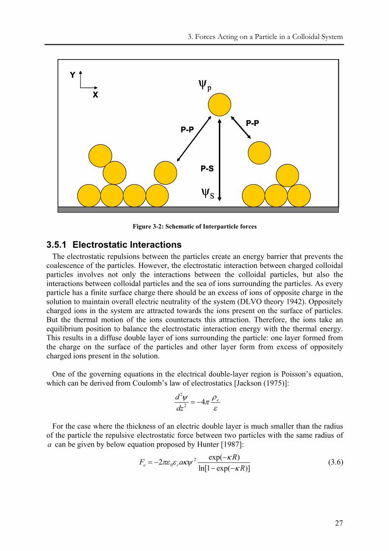
3.5 Interparticle forces The interparticle forces can be estimated by using the DLVO theory. This theory is a very
good approximation for low concentrated solutions. According to this theory the major long-range interaction forces acting on two approaching particles are electrostatic force, eF , and van der Waals force, vdWF . (Figure 3-2)
3. Forces Acting on a Particle in a Colloidal System
27
P-P
P-S
P-P
Y
Xpψ
Sψ
P-P
P-S
P-P
Y
Xpψ
Sψ
Figure 3-2: Schematic of Interparticle forces
3.5.1 Electrostatic Interactions The electrostatic repulsions between the particles create an energy barrier that prevents the
coalescence of the particles. However, the electrostatic interaction between charged colloidal particles involves not only the interactions between the colloidal particles, but also the interactions between colloidal particles and the sea of ions surrounding the particles. As every particle has a finite surface charge there should be an excess of ions of opposite charge in the solution to maintain overall electric neutrality of the system (DLVO theory 1942). Oppositely charged ions in the system are attracted towards the ions present on the surface of particles. But the thermal motion of the ions counteracts this attraction. Therefore, the ions take an equilibrium position to balance the electrostatic interaction energy with the thermal energy. This results in a diffuse double layer of ions surrounding the particle: one layer formed from the charge on the surface of the particles and other layer form from excess of oppositely charged ions present in the solution.
One of the governing equations in the electrical double-layer region is Poisson’s equation, which can be derived from Coulomb’s law of electrostatics [Jackson (1975)]:
2
2 4 eddz
ρψ πε
= −
For the case where the thickness of an electric double layer is much smaller than the radius of the particle the repulsive electrostatic force between two particles with the same radius of a can be given by below equation proposed by Hunter [1987]:
20
exp( )2ln[1 exp( )]e r
RF aR
κπε ε κψκ
−= −
− − (3.6)
Produced Water Re-Injection
28
Where 12 2 -1 -10 8.85 10 C J mε −= × is the absolute permittivity of the free space, rε the
dielectric constant of the fluid between particle (for water: 78.5), ψ Stern potential, and κ the reciprocal of the thickness double layer. The measurable value of zeta potential ξ can be used for most conditions instead of , and the κ can be estimated by:
1/ 22 0 2
0
i i
r B
e n zk T
κε ε
⎡ ⎤= ⎢ ⎥⎢ ⎥⎣ ⎦
∑ (3.7)
Where e is the electrical charge ( 191.6 10 C−× ), 0in and iz are the number of ions per unit
volume in the bulk solution and valence of type I, respectively, Bk the Boltzmann constant ( 23 -11.4 10 J K−= × ) and T is the absolute temperature in Kelvin.
Tent and Nijenhuis [1992] obtained the shortest distance R between two neighboring particles by proposing a hexagonal packing structure of the deposited particles:
0.33
1 0
1(1 ) pR d
Kπε
⎧ ⎫⎡ ⎤⎪ ⎪= −⎨ ⎬⎢ ⎥−⎣ ⎦⎪ ⎪⎩ ⎭ (3.8)
McDonogh et al. [1994] indicated that the only interparticle forces between neighboring particles of filter cake should be considered. The proposed the following equation to evaluate
1K with assuimg the hexagonal packing straucture of the deposited particles:
1 3cosK θ= (3.9)
θ varies from 0 to 90 and for hexagonal packing θ is 54.7 .
3.5.2 Van der Waals Forces Van der Waals attractive forces (or London dispersion forces) are weak forces that exist
between uncharged molecules as a result of polarity. These forces become significant when sizes of the particles are very small and the distances are in nano level. It is important to remember that van der Waals' forces are forces that exist between molecules of the same substance. They are quite different from the forces that make up the molecule. For example, a water molecule is made up of hydrogen and oxygen, which are bonded together by the sharing of electrons. These electrostatic forces that keep a molecule intact are existent in covalent and ionic bonding but they are not van der Waals' forces.
The origin of the van der Waals attractions may be related to the fluctuations in the charge distribution of atoms. It is important to note that electrons are constantly moving within a bond. There are moments that electrons are crowded in one side. This gives a temporary polarity to the atom. This induces polarity to the adjacent atom by repelling the electron cloud. However, this temporary charge disappears as quickly as it appeared because the electrons are moving so fast. According to the theory of London [1930], the attractive forces between atoms are additive in nature. Because of this nature, the attractive interaction between two colloidal particles containing many atoms is appreciable.
3. Forces Acting on a Particle in a Colloidal System
29
The Van der Waals attractive forces between atoms are very small. Hamaker [1937] derived an expression for the attractive interaction between colloidal particles. For two particles of radii 1 2 and a a separated by distance r , the Van de Waals potential energy is given by:
2
1 2 1 2 1 22 2 2
1 2
2 2 4( ) ln( )6 4VdW
a a a a r a aAU rr a a r r
⎛ ⎞−−= + +⎜ ⎟−⎝ ⎠
(3.10)
For two particles of the same size and when the distance between particle surfaces much less than the radius of particle, equation () becomes:
1( )12 2VdWAaU r
r a−
=−
(3.11)
A is the Hamaker constant which has values generally in order of Jouls.
To calculate the van der Waals force we put: ( )VdWvdW
U rFr
∂=
∂. Then for the particles with
identical diameter of pd , van der Waals that we assumed to be the main source of attraction between colloidal molecules can be calculated with the following equation:
( )2
1( )24
pvdW
p
AdF r
r d
−=
− (3.12)
Van der Waals attraction forces can be calculated by the formula proposed by Hunter, regarding the condition that the thickness of the double layer is much smaller than the diameter of the particles:
6
2 2 36 ( 2 ) ( )p
vdWp p
AdF
R R d R d= −
+ + (3.13)
3.6 Diffusion 3.6.1 Brownian Diffusion
In crossflow filtration permeate flux drags particles towards the filter medium, but from the other side the crossflow induces particles backtransport into the bulk. Belfort et al. [1994] have proposed that besides inertial lift, diffusion of the particles helps to the backtransport of the particles. Trettin and Doshi [1980] solved the governing convective-diffusion equation for crossflow filtration assuming that diffusion is the only mechanism of backtransport of the particles and proposed the following equation for the length averaged permeate flux, J for dilute suspensions:
1/3 1/30, 00.81( / ) ( / )w Bo w bJ D Lτ µ= Φ Φ (3.14)
Where wτ is the wall shear stress, 0µ the permeate viscosity, L the filter length, wΦ the particle volume fraction at the filter surface, and bΦ the particle volume fraction in the bulk.
0,BoD is the Brownian diffusion coefficient for dilute suspensions of spheres, which is given by Stokes-Einestein equation:
Produced Water Re-Injection
30
0, 0/ 6Bo BD k T aπµ= (3.15)
Here a is the particle radius.
3.6.2 Shear induced diffusion Shear induced hydrodynamic diffusion of particles occurs because individual particles
undergo random displacements from the streamlines in a shear flow as they interact with and tumble over other particles [Belfort (1994)]. The shear induced diffusion coefficient can be calculated from the formula suggested by Eckstein et al. [1977]:
20.3s wD aτ= (3.16)
Equation indicates that the shear induced hydrodynamic diffusivity is proportional to the square of the particle size by the shear rate. It is evident from the comparison of (3.15) and (3.16) that unlike shear induced hydrodynamic diffusivity, Brownian diffusivity is independent of the shear rate. As a result Brownian diffusivity is important for low shear rates and sub-micron particle, whereas in the larger particles and higher shear rates shear induced hydrodynamic diffusivity is dominant. The resulting particle migration by shear induced diffusion can be calculated by using an effective diffusion coefficient (Leighton and Acrivos, 1986-7):
2 20.33 (1 0.5exp(8.8 )) /SI wD aτ µ= Φ + Φ (3.17)
Numerical calculations of shear-induced diffusion have been performed by Davis and Sherwood [1990] . For low particle concentrations and max 0.58Φ = they found that:
4 1/3
0
0.06 ( / )wbJ a Lτ
µ= Φ (3.18)
3.7 Friction Force Coulomb conducted hundreds of experiments with different material in broad range of
conditions. He found out that the magnitude of frictional force is proportional to the sum of normal forces.
.f NF f F=
The proportionality, f , is called Coulomb’s frictional coefficient. Coulomb found out that frictional force is approximately independent of contact area and velocity magnitude. In a colloidal system frictional force can be written as:
( )f D e GF f F F F= + + (3.19)
where, fF is the frictional force, DF the drag force of permeate velocity, eF electrostatic forces and GF represents the net gravity force.
3. Forces Acting on a Particle in a Colloidal System
31
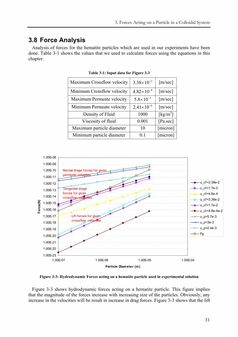
3.8 Force Analysis Analysis of forces for the hematite particles which are used in our experiments have been
done. Table 3-1 shows the values that we used to calculate forces using the equations in this chapter.
Table 3-1: Input data for Figure 3-3
Maximum Crossflow velocity 23.38 10−× [m/sec]
Minimum Crossflow velocity 44.82 10−× [m/sec] Maximum Permeate velocity 35.8 10−× [m/sec] Minimum Permeate velocity 42.41 10−× [m/sec]
Density of Fluid 1000 [kg/m3] Viscosity of fluid 0.001 [Pa.sec]
Maximum particle diameter 10 [micron] Minimum particle diameter 0.1 [micron]
1.00E-23
1.00E-22
1.00E-21
1.00E-20
1.00E-19
1.00E-18
1.00E-17
1.00E-16
1.00E-15
1.00E-14
1.00E-13
1.00E-12
1.00E-11
1.00E-10
1.00E-09
1.00E-08
1.00E-07 1.00E-06 1.00E-05 1.00E-04
Particle Diameter (m)
Forc
e(N
)
u_cf=3.38e-2
u_cf=1.7e-2
u_cf=4.8e-4
u_cf=3.38e-2
u_cf=1.7e-2
u_cf=4.8e-4e-2
u_p=5.7e-3
u_p=3e-3
u_p=2.4e-3
Fg
Normal drage forces for given permeate velocities
Lift forces for given crossflow velocities
Tangential drage forces for given crossflow velocities
Figure 3-3: Hydrodynamic Forces acting on a hematite particle used in experimental solution
Figure 3-3 shows hydrodynamic forces acting on a hematite particle. This figure implies
that the magnitude of the forces increase with increasing size of the particles. Obviously, any increase in the velocities will be result in increase in drag forces. Figure 3-3 shows that the lift

Produced Water Re-Injection
32
force compared to the drag force is negligible and we can ignore the lift force in our force balance. Net gravity force becomes important with larger particles and can not be ignored.
33
CHAPTER 4
4 EXTERNAL CAKE
4.1 Introduction In 1907 Bechhold [1907] found out that at the filtration process with flow parallel to the
filter medium (crossflow) the volume of filtrate can be increased before a compact cake layer completely blocks the pores of the filter. The phenomena may occur during activities in which a suspension flows tangentially to some porous media, e.g. fluid loss from a drilling mud or flow of injected fluids in fractures resulting in formation of the external cake.
Crossflow filtration refers to a pressure driven separation process in which the permeate flow is perpendicular to the feed flow. In other words in crossflow filtration the main direction of suspension flow is perpendicular to the flow direction of the recovered (or separated) liquid. The term crossflow just describes the direction of the fluid and does not describe the type of medium where particles are deposited. Different parameters affect the crossflow filtration e.g. crossflow velocity, transmembrane pressure, membrane resistance, layer resistance, size distribution of the suspended particles, particle form, agglomeration behavior and surface effects of the particles. However, the main and central issue for all investigation about crossflow filtration is: How does one estimate the fraction of particles transported to membrane surface associated with the permeating liquid become deposited. It is obvious that the particles that come to the surface of membrane just a fraction of them become deposited.
In petroleum industry transport of fluid containing particles in the subsurface is similar to crossflow filtration. For example in the fractures, transport of injected fluid will result in formation of cake on the surface of the rock. Another example is the build up of mud cake during the drilling of well. Therefore, external cake build-up is another important phenomena that should be investigated in order to predict the extent of the damage. Dynamic or crossflow
Produced Water Re-Injection
34
filtration is important because the erosive effects associated with flow limit the build-up of the external filter cake that was predicted by static filtration.
In this chapter, using Navier-Stokes equations and force balance a novel model is developed. Based on these equations we made a simulator which can give the profile of external cake.
It should be noted that Prof. Bedrikovetsky was the motivator of undertaking the external filter cake study. The basis of the following work was formulated by Profs. Bedrikovetsy and Currie, and the presented work was developed by Al-Abduwani and the author (Farjzadeh).
4.2 Experimental Setup
xy
X
X
ψψ
ζξ 0ψ =ξ
W
hH
( )pu x( )pu x
zy
Cross-section XX
wP
0P
lP
xy
X
X
ψψ
ζξ 0ψ =ξ
WW
hH
( )pu x( )pu x
zy
Cross-section XX
wP
0P
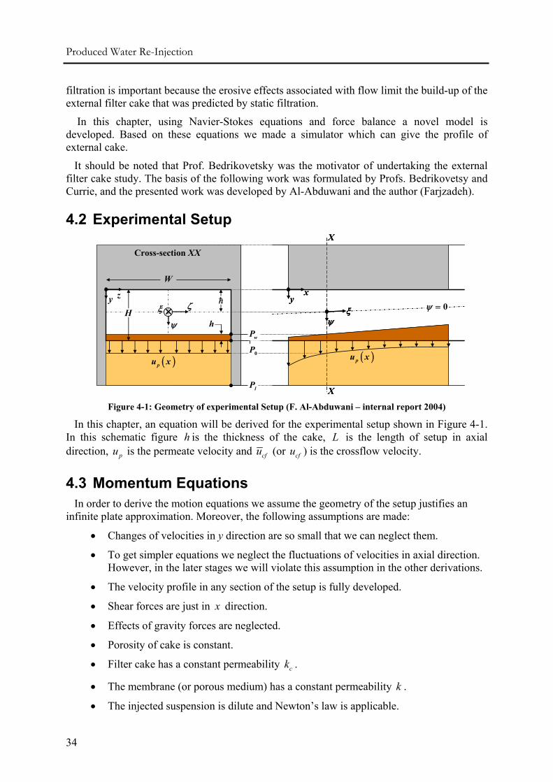
lP Figure 4-1: Geometry of experimental Setup (F. Al-Abduwani – internal report 2004)
In this chapter, an equation will be derived for the experimental setup shown in Figure 4-1. In this schematic figure h is the thickness of the cake, L is the length of setup in axial direction, pu is the permeate velocity and cfu (or cfu ) is the crossflow velocity.
4.3 Momentum Equations In order to derive the motion equations we assume the geometry of the setup justifies an
infinite plate approximation. Moreover, the following assumptions are made:
• Changes of velocities in y direction are so small that we can neglect them.
• To get simpler equations we neglect the fluctuations of velocities in axial direction. However, in the later stages we will violate this assumption in the other derivations.
• The velocity profile in any section of the setup is fully developed.
• Shear forces are just in x direction.
• Effects of gravity forces are neglected.
• Porosity of cake is constant.
• Filter cake has a constant permeability ck .
• The membrane (or porous medium) has a constant permeability k .
• The injected suspension is dilute and Newton’s law is applicable.
4. External Cake
35
With these assumptions the boundary conditions of the problem are:
0
0dud ψψ =
= (4.1)
0 at 2cf
H hu ψ −= = = (4.2)
Thus, solving of the momentum equation follows:
22
. . 12cf
dpudx
ψµ
⎡ ⎤⎛ ⎞= − −⎢ ⎥⎜ ⎟⎝ ⎠⎢ ⎥⎣ ⎦
(4.3)
Average crossflow velocity can be calculated with:
2
3cfdpudxµ
=− (4.4)
Shear stress in the transverse direction ψ is given by:
( ) 2
3.cfu
ψ
µτ ψ ψ= (4.5)
(4.5) is used to calculate shear stress at the surface of the cake as:
( )3 cfu
ψ
µτ ψ = (4.6)
To calculate the velocity in y direction Darcy’s law is applied:
ip
k puyµ
∂=∂
(4.7)
Applying Darcy’s law to the two separate media, the membrane and the cake itself, yields:
puhΨ=+Θ
(4.8)
with
( )c w lk p pµ−
Ψ= (4.9)
and
ck lk
Θ= (4.10)
It should be noticed that ψ is not constant along the channel, because according to (4.4) pressure is not constant along the channel.
4.4 Forces acting on a particle on the surface of cake
Produced Water Re-Injection
36
4.4.1 Tangential Drag Force: The tangential drag force can be calculated by one of three ways:
4.4.1.1 Poiseuille’s Law For Infinite Plate:
( )
224 cfd
uF a
H hµ
π=−
(4.11)
4.4.1.2 Poiseuille’s Law for Equivalent Tube:
( )
216 .d cfF a uW H h
ππ µ=−
(4.12)
4.4.1.3 Stokes law:
( )
218 cfd
uF a
H hµ
π=−
(4.13)
4.4.1.4 General Form of the Tangential Drag Force:
( )
2 cfd
uF a
H hµ
απ=−
(4.14)
α will be determined depending on the method we use to calculate the tangential drag force.
4.4.2 Normal Drag Force: The normal drag force acts on a particle due to permeate velocity and can be calculated
using Stoke’s law:
6r pF auπµ= (4.15)
4.4.3 Electrostatic Forces According to DLVO theory there are two main electrostatic forces acting on a particle:
double layer forces and Van der Waals forces.
4.4.4 Frictional Force .f Nf f F= (4.16)
4.5 Solving for the Force Balance Equality During a crossflow filtration process particle will be deposited if friction force overcomes
the tangential drag force. Therefore, while the tangential force overcomes the friction force, cake reaches its critical or equilibrium thickness and forces satisfy the inequality:
( )D e r GF f F F F≥ + + (4.17)
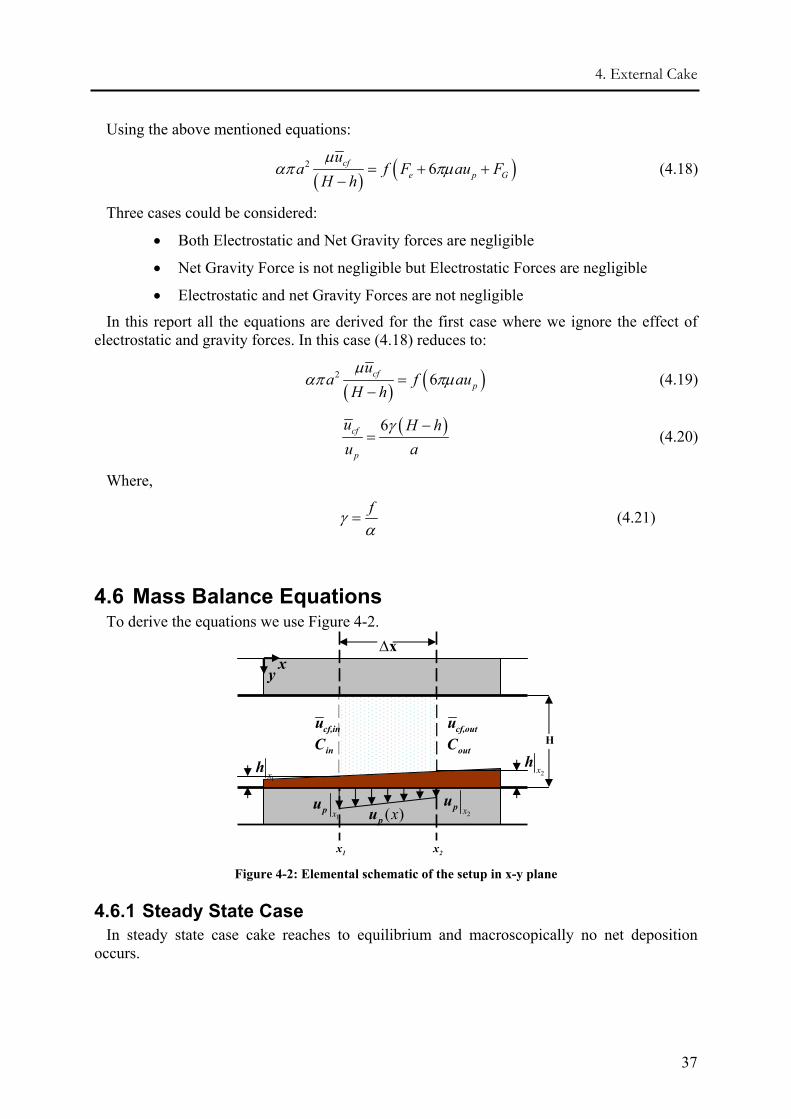
4. External Cake
37
Using the above mentioned equations:
( ) ( )2 6cf
e p G
ua f F au F
H hµ
απ πµ= + +−
(4.18)
Three cases could be considered:
• Both Electrostatic and Net Gravity forces are negligible
• Net Gravity Force is not negligible but Electrostatic Forces are negligible
• Electrostatic and net Gravity Forces are not negligible
In this report all the equations are derived for the first case where we ignore the effect of electrostatic and gravity forces. In this case (4.18) reduces to:
( ) ( )2 6cf
p
ua f au
H hµ
απ πµ=−
(4.19)
( )6cf
p
u H hu a
γ −= (4.20)
Where,
fγα
= (4.21)
4.6 Mass Balance Equations To derive the equations we use Figure 4-2.
Figure 4-2: Elemental schematic of the setup in x-y plane
4.6.1 Steady State Case In steady state case cake reaches to equilibrium and macroscopically no net deposition
occurs.
H
∆xx
y
cf,inuinC
cf,outuoutC
1x 2x
( )xpu
1xh 2x
h
1xpu
2xpu
Produced Water Re-Injection
38
4.6.1.1 Mass Balance Equation for Fluid Phase
( )cf
p
u H hu
x
⎡ ⎤∂ −⎣ ⎦= −∂
(4.22)
4.6.1.2 Mass Balance Equation for Particles
( )2
dc a dxc H h=
− (4.23)
4.6.1.3 Equation for the Pressure Change along the Channel Replacing (4.20) into (4.4) follows:
( )( )
72dpdx a H h h
γµψ= −
− +Θ (4.24)
(4.24) is valid for both transient and steady state cases.
4.6.1.4 Equation for the Thickness of Cake
722
p c
cf p
u kdh hdx h H u a u
γ ψ⎡ ⎤+Θ⎡ ⎤= −⎢ ⎥⎢ ⎥+ Θ+⎣ ⎦ ⎢ ⎥⎣ ⎦ (4.25)
To calculate the thickness of cake in a given flow boundary we can use the following equation:
( )( )24
12
Qa Qa Qa W Hh H
W
γ ψ
γ ψ
± + +Θ= + (4.26)
4.6.2 Transient Case with Erosion In filtration the rate of cake height growth can be obtained from mass balance for particles.
Mass balance for the particle mass flow in Figure 4-3 can be written as:
, ,p
p in p back
dVV V
dt− = (4.27)
(4.27) indicates that the change of control volume equals to the volume of deposited particles minus the volume of eroded ones.
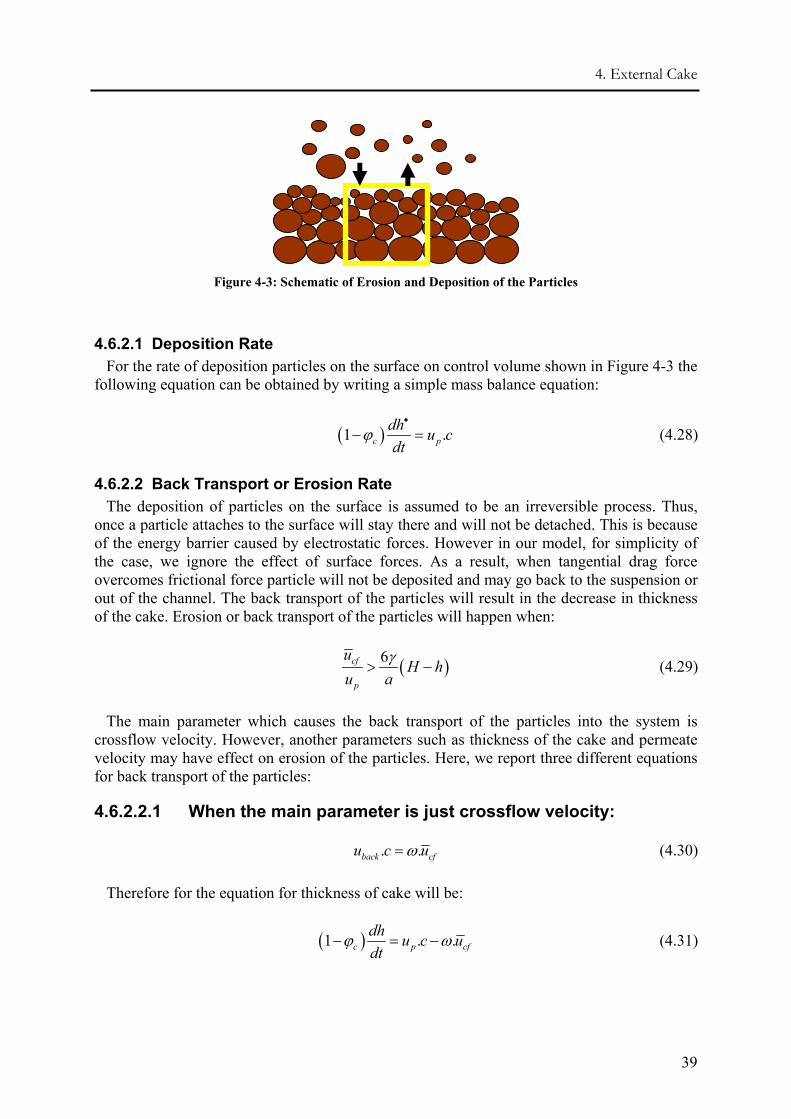
4. External Cake
39
Figure 4-3: Schematic of Erosion and Deposition of the Particles
4.6.2.1 Deposition Rate For the rate of deposition particles on the surface on control volume shown in Figure 4-3 the
following equation can be obtained by writing a simple mass balance equation:
( )1 .c pdh u cdt
ϕ•
− = (4.28)
4.6.2.2 Back Transport or Erosion Rate The deposition of particles on the surface is assumed to be an irreversible process. Thus,
once a particle attaches to the surface will stay there and will not be detached. This is because of the energy barrier caused by electrostatic forces. However in our model, for simplicity of the case, we ignore the effect of surface forces. As a result, when tangential drag force overcomes frictional force particle will not be deposited and may go back to the suspension or out of the channel. The back transport of the particles will result in the decrease in thickness of the cake. Erosion or back transport of the particles will happen when:
( )6cf
p
uH h
u aγ
> − (4.29)
The main parameter which causes the back transport of the particles into the system is crossflow velocity. However, another parameters such as thickness of the cake and permeate velocity may have effect on erosion of the particles. Here, we report three different equations for back transport of the particles:
4.6.2.2.1 When the main parameter is just crossflow velocity:
. .back cfu c uω= (4.30)
Therefore for the equation for thickness of cake will be:
( )1 . .c p cfdh u c udt
ϕ ω− = − (4.31)
Produced Water Re-Injection
40
ω is the proportionality coefficient and may be called “Erosion Coefficient” and assumed to be constant along the channel. Erosion coefficient can be calculated by applying (4.31) for steady state case when time derivative of height is zero and averaging it along the core:
SS
p
cf
uMEAN c
uω
⎡ ⎤⎛ ⎞⎢ ⎥= ⎜ ⎟⎜ ⎟⎢ ⎥⎝ ⎠⎣ ⎦
(4.32)
4.6.2.2.2 When both crossflow velocity and height of cake are important parameters
( )
.m
cfback n
uu c
H hω=
− (4.33)
then,
( )( )
1 . .m
cfc p n
udh u cdt H h
ϕ ω− = −−
(4.34)
with:
( ) 1
1
.6
n
mcf SS
a H h cMEAN
uω
γ
−
−
⎡ ⎤⎛ ⎞−⎢ ⎥⎜ ⎟=⎜ ⎟⎢ ⎥⎝ ⎠⎣ ⎦
(4.35)
When m=n=1, we have:
( )1 . . cfc p
udh u cdt H h
ϕ ω− = −−
(4.36)
with:
.6 SS
a cMEANωγ
⎡ ⎤⎛ ⎞= ⎢ ⎥⎜ ⎟
⎝ ⎠⎣ ⎦ (4.37)
Although it is initially assumed that erosion is independent of initial concentration of the
particles in the suspensions, the final equations for ω shows the dependency of erosion on concentration.
4.6.2.3 Mass Balance Equation for Fluid Writing mass balance equation for fluid in the suspension and also in the cake will lead to the following equation:
( ) ( )1cf c
p
u H h H hu
x tϕ⎡ ⎤∂ − ∂ − −⎡ ⎤⎣ ⎦ ⎣ ⎦− = +
∂ ∂ (4.38)
4.6.2.4 Mass Balance Equation for Particles
In this case we will get an equation for concentration. Mass balance is written for particles in the suspension as well as the cake.
4. External Cake
41
( ) ( ) ( ). 1cf cC hH h C u H h Ct x t
ϕ∂ ∂ ∂⎡ ⎤⎡ ⎤− = − − + − −⎣ ⎦⎢ ⎥∂ ∂ ∂⎣ ⎦ (4.39)
All of the above equations are solved numerically and put in the simulator to build the profiles of cake thickness and velocities. This will be explained in details in chapter 7.

Produced Water Re-Injection
42
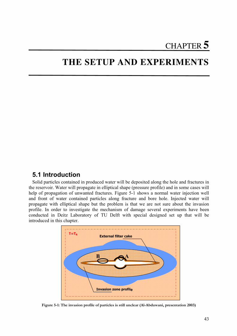
43
CHAPTER 5
5 THE SETUP AND EXPERIMENTS
5.1 Introduction Solid particles contained in produced water will be deposited along the hole and fractures in
the reservoir. Water will propagate in elliptical shape (pressure profile) and in some cases will help of propagation of unwanted fractures. Figure 5-1 shows a normal water injection well and front of water contained particles along fracture and bore hole. Injected water will propagate with elliptical shape but the problem is that we are not sure about the invasion profile. In order to investigate the mechanism of damage several experiments have been conducted in Deitz Laboratory of TU Delft with special designed set up that will be introduced in this chapter.
TT==TTRR
Invasion zone profil
External filter cake
Figure 5-1: The invasion profile of particles is still unclear (Al-Abduwani, presentation 2003)
A B
e
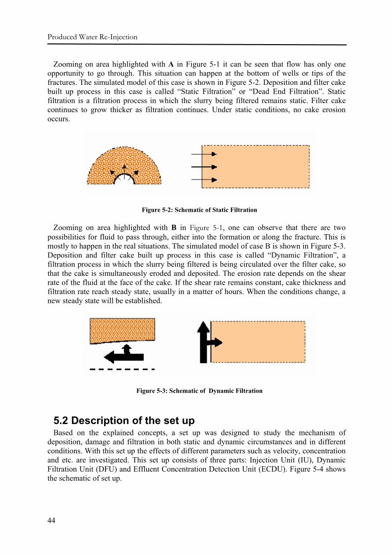
Produced Water Re-Injection
44
Zooming on area highlighted with A in Figure 5-1 it can be seen that flow has only one opportunity to go through. This situation can happen at the bottom of wells or tips of the fractures. The simulated model of this case is shown in Figure 5-2. Deposition and filter cake built up process in this case is called “Static Filtration” or “Dead End Filtration”. Static filtration is a filtration process in which the slurry being filtered remains static. Filter cake continues to grow thicker as filtration continues. Under static conditions, no cake erosion occurs.
Figure 5-2: Schematic of Static Filtration
Zooming on area highlighted with B in Figure 5-1, one can observe that there are two possibilities for fluid to pass through, either into the formation or along the fracture. This is mostly to happen in the real situations. The simulated model of case B is shown in Figure 5-3. Deposition and filter cake built up process in this case is called “Dynamic Filtration”, a filtration process in which the slurry being filtered is being circulated over the filter cake, so that the cake is simultaneously eroded and deposited. The erosion rate depends on the shear rate of the fluid at the face of the cake. If the shear rate remains constant, cake thickness and filtration rate reach steady state, usually in a matter of hours. When the conditions change, a new steady state will be established.
Figure 5-3: Schematic of Dynamic Filtration
5.2 Description of the set up Based on the explained concepts, a set up was designed to study the mechanism of
deposition, damage and filtration in both static and dynamic circumstances and in different conditions. With this set up the effects of different parameters such as velocity, concentration and etc. are investigated. This set up consists of three parts: Injection Unit (IU), Dynamic Filtration Unit (DFU) and Effluent Concentration Detection Unit (ECDU). Figure 5-4 shows the schematic of set up.
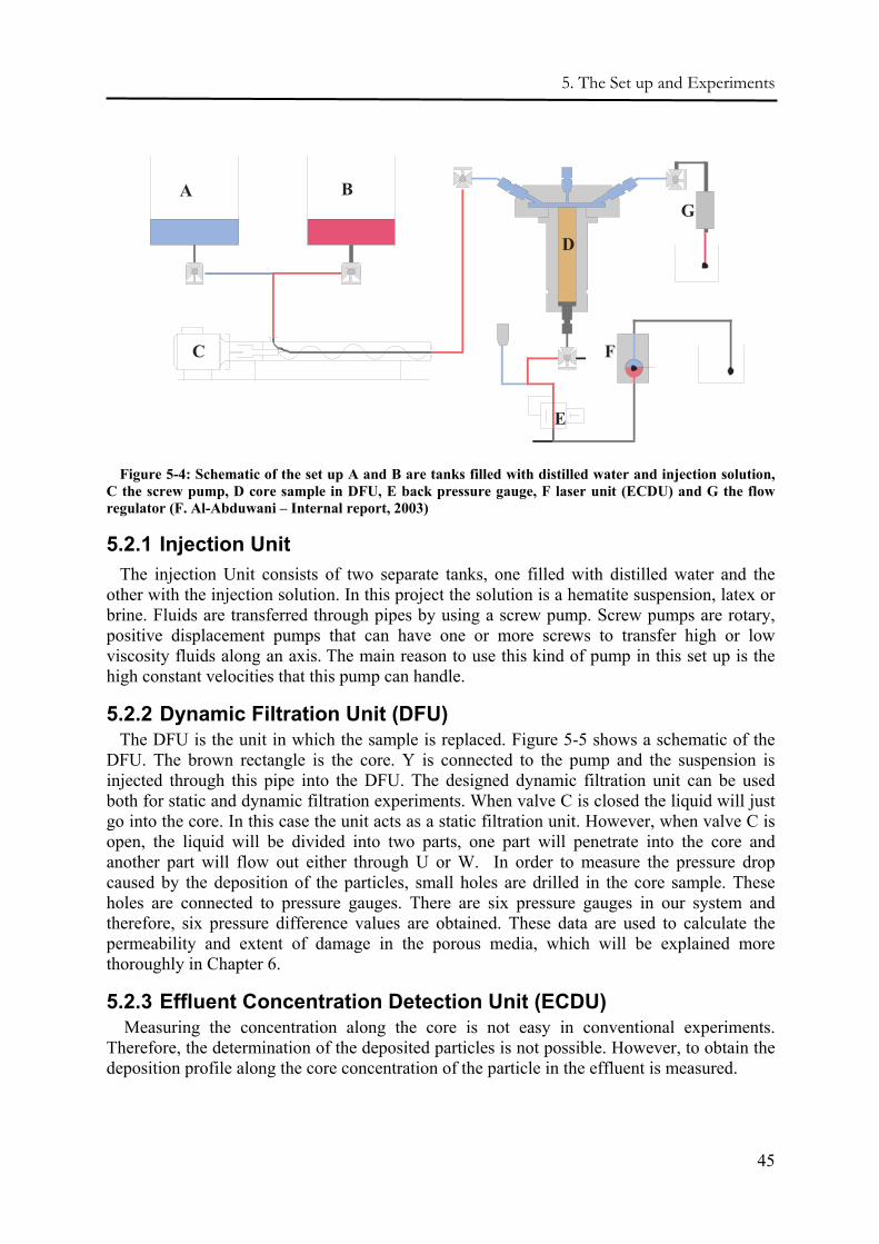
5. The Set up and Experiments
45
A B
C
D
E
F
G
Figure 5-4: Schematic of the set up A and B are tanks filled with distilled water and injection solution, C the screw pump, D core sample in DFU, E back pressure gauge, F laser unit (ECDU) and G the flow regulator (F. Al-Abduwani – Internal report, 2003)
5.2.1 Injection Unit The injection Unit consists of two separate tanks, one filled with distilled water and the
other with the injection solution. In this project the solution is a hematite suspension, latex or brine. Fluids are transferred through pipes by using a screw pump. Screw pumps are rotary, positive displacement pumps that can have one or more screws to transfer high or low viscosity fluids along an axis. The main reason to use this kind of pump in this set up is the high constant velocities that this pump can handle.
5.2.2 Dynamic Filtration Unit (DFU) The DFU is the unit in which the sample is replaced. Figure 5-5 shows a schematic of the
DFU. The brown rectangle is the core. Y is connected to the pump and the suspension is injected through this pipe into the DFU. The designed dynamic filtration unit can be used both for static and dynamic filtration experiments. When valve C is closed the liquid will just go into the core. In this case the unit acts as a static filtration unit. However, when valve C is open, the liquid will be divided into two parts, one part will penetrate into the core and another part will flow out either through U or W. In order to measure the pressure drop caused by the deposition of the particles, small holes are drilled in the core sample. These holes are connected to pressure gauges. There are six pressure gauges in our system and therefore, six pressure difference values are obtained. These data are used to calculate the permeability and extent of damage in the porous media, which will be explained more thoroughly in Chapter 6.
5.2.3 Effluent Concentration Detection Unit (ECDU) Measuring the concentration along the core is not easy in conventional experiments.
Therefore, the determination of the deposited particles is not possible. However, to obtain the deposition profile along the core concentration of the particle in the effluent is measured.
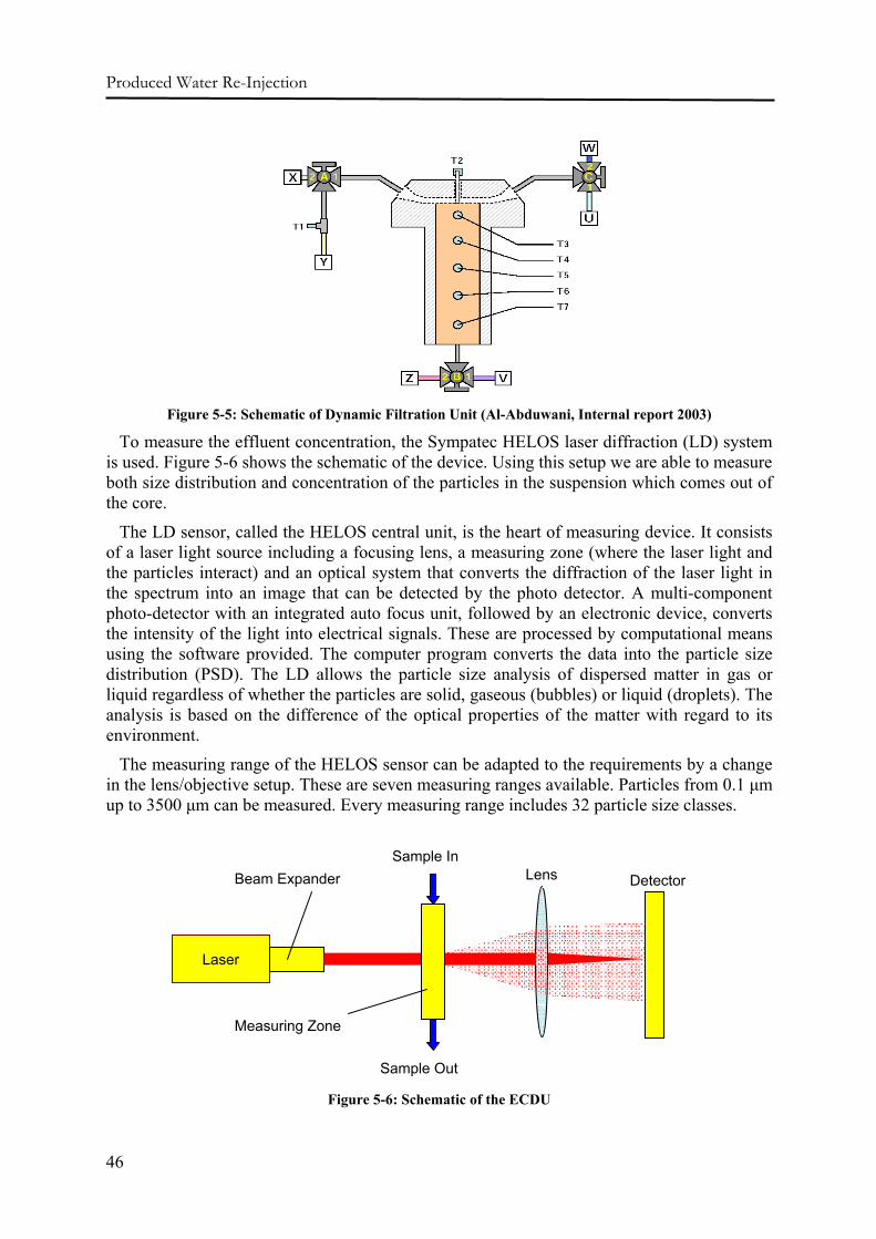
Produced Water Re-Injection
46
Figure 5-5: Schematic of Dynamic Filtration Unit (Al-Abduwani, Internal report 2003)
To measure the effluent concentration, the Sympatec HELOS laser diffraction (LD) system is used. Figure 5-6 shows the schematic of the device. Using this setup we are able to measure both size distribution and concentration of the particles in the suspension which comes out of the core.
The LD sensor, called the HELOS central unit, is the heart of measuring device. It consists of a laser light source including a focusing lens, a measuring zone (where the laser light and the particles interact) and an optical system that converts the diffraction of the laser light in the spectrum into an image that can be detected by the photo detector. A multi-component photo-detector with an integrated auto focus unit, followed by an electronic device, converts the intensity of the light into electrical signals. These are processed by computational means using the software provided. The computer program converts the data into the particle size distribution (PSD). The LD allows the particle size analysis of dispersed matter in gas or liquid regardless of whether the particles are solid, gaseous (bubbles) or liquid (droplets). The analysis is based on the difference of the optical properties of the matter with regard to its environment.
The measuring range of the HELOS sensor can be adapted to the requirements by a change in the lens/objective setup. These are seven measuring ranges available. Particles from 0.1 µm up to 3500 µm can be measured. Every measuring range includes 32 particle size classes.
Figure 5-6: Schematic of the ECDU
Laser
Beam Expander Sample In
Sample Out
Measuring Zone
Lens Detector
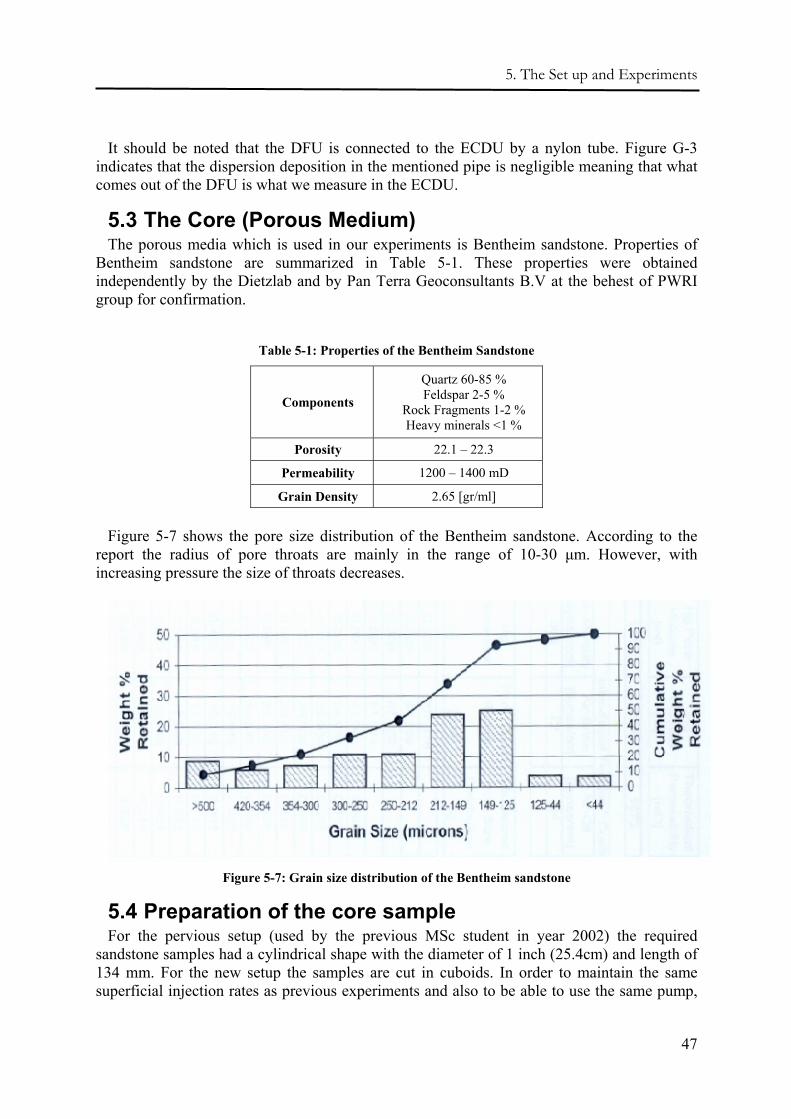
5. The Set up and Experiments
47
It should be noted that the DFU is connected to the ECDU by a nylon tube. Figure G-3 indicates that the dispersion deposition in the mentioned pipe is negligible meaning that what comes out of the DFU is what we measure in the ECDU.
5.3 The Core (Porous Medium) The porous media which is used in our experiments is Bentheim sandstone. Properties of
Bentheim sandstone are summarized in Table 5-1. These properties were obtained independently by the Dietzlab and by Pan Terra Geoconsultants B.V at the behest of PWRI group for confirmation.
Table 5-1: Properties of the Bentheim Sandstone
Components
Quartz 60-85 % Feldspar 2-5 %
Rock Fragments 1-2 % Heavy minerals <1 %
Porosity 22.1 – 22.3
Permeability 1200 – 1400 mD
Grain Density 2.65 [gr/ml]
Figure 5-7 shows the pore size distribution of the Bentheim sandstone. According to the
report the radius of pore throats are mainly in the range of 10-30 µm. However, with increasing pressure the size of throats decreases.
Figure 5-7: Grain size distribution of the Bentheim sandstone
5.4 Preparation of the core sample For the pervious setup (used by the previous MSc student in year 2002) the required
sandstone samples had a cylindrical shape with the diameter of 1 inch (25.4cm) and length of 134 mm. For the new setup the samples are cut in cuboids. In order to maintain the same superficial injection rates as previous experiments and also to be able to use the same pump,
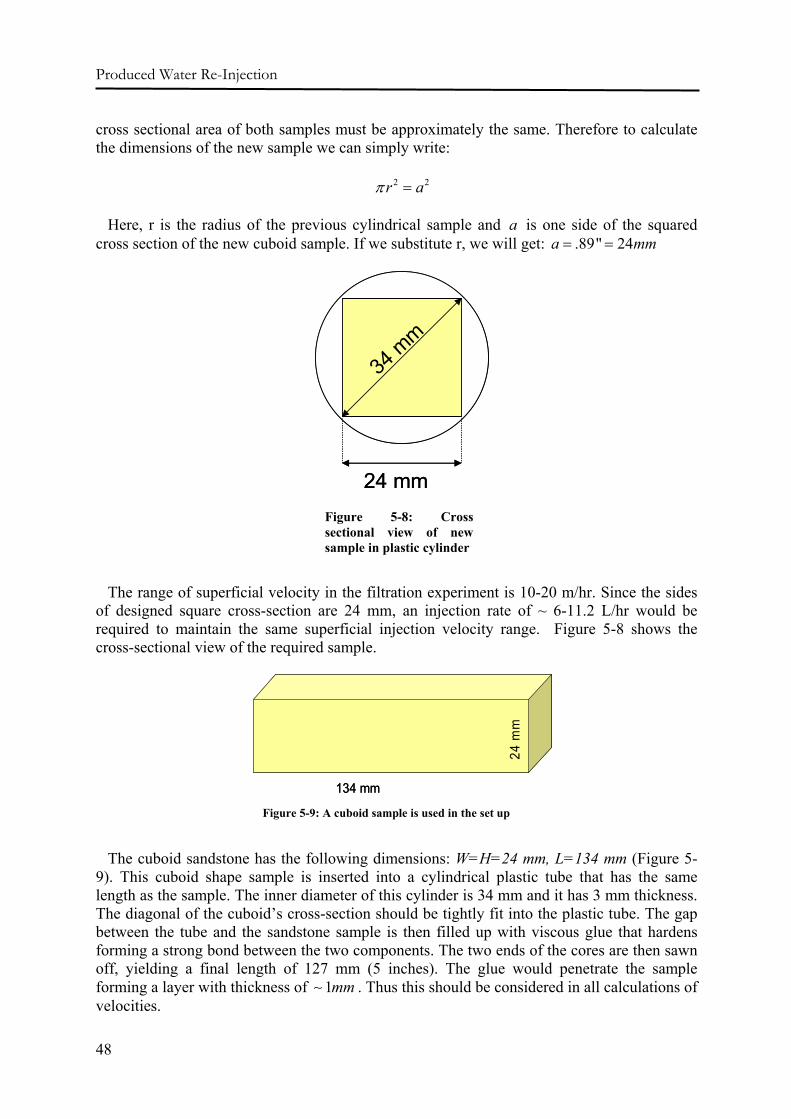
Produced Water Re-Injection
48
cross sectional area of both samples must be approximately the same. Therefore to calculate the dimensions of the new sample we can simply write:
2 2r aπ =
Here, r is the radius of the previous cylindrical sample and a is one side of the squared cross section of the new cuboid sample. If we substitute r, we will get: .89" 24a mm= =
The range of superficial velocity in the filtration experiment is 10-20 m/hr. Since the sides of designed square cross-section are 24 mm, an injection rate of ~ 6-11.2 L/hr would be required to maintain the same superficial injection velocity range. Figure 5-8 shows the cross-sectional view of the required sample.
The cuboid sandstone has the following dimensions: W=H=24 mm, L=134 mm (Figure 5-9). This cuboid shape sample is inserted into a cylindrical plastic tube that has the same length as the sample. The inner diameter of this cylinder is 34 mm and it has 3 mm thickness. The diagonal of the cuboid’s cross-section should be tightly fit into the plastic tube. The gap between the tube and the sandstone sample is then filled up with viscous glue that hardens forming a strong bond between the two components. The two ends of the cores are then sawn off, yielding a final length of 127 mm (5 inches). The glue would penetrate the sample forming a layer with thickness of 1mm∼ . Thus this should be considered in all calculations of velocities.
34 m
m
24 mm
34 m
m
24 mmFigure 5-8: Cross sectional view of new sample in plastic cylinder
134 mm
24 m
m
134 mm
24 m
m
Figure 5-9: A cuboid sample is used in the set up
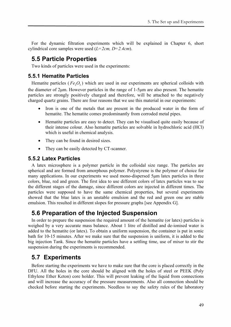
5. The Set up and Experiments
49
For the dynamic filtration experiments which will be explained in Chapter 6, short cylindrical core samples were used (L=2cm, D=2.4cm).
5.5 Particle Properties Two kinds of particles were used in the experiments:
5.5.1 Hematite Particles Hematite particles ( 2 3Fe O ) which are used in our experiments are spherical colloids with
the diameter of 2µm. However particles in the range of 1-5µm are also present. The hematite particles are strongly positively charged and therefore, will be attached to the negatively charged quartz grains. There are four reasons that we use this material in our experiments:
• Iron is one of the metals that are present in the produced water in the form of hematite. The hematite comes predominantly from corroded metal pipes.
• Hematite particles are easy to detect. They can be visualised quite easily because of their intense colour. Also hematite particles are solvable in hydrochloric acid (HCl) which is useful in chemical analysis.
• They can be found in desired sizes.
• They can be easily detected by CT-scanner.
5.5.2 Latex Particles A latex microsphere is a polymer particle in the colloidal size range. The particles are
spherical and are formed from amorphous polymer. Polystyrene is the polymer of choice for many applications. In our experiments we used mono-dispersed 5µm latex particles in three colors, blue, red and green. The first idea to use different colors of latex particles was to see the different stages of the damage, since different colors are injected in different times. The particles were supposed to have the same chemical properties, but several experiments showed that the blue latex is an unstable emulsion and the red and green one are stable emulsion. This resulted in different slopes for pressure graphs [see Appendix G].
5.6 Preparation of the Injected Suspension In order to prepare the suspension the required amount of the hematite (or latex) particles is
weighed by a very accurate mass balance. About 1 litre of distilled and de-ionised water is added to the hematite (or latex). To obtain a uniform suspension, the container is put in sonic bath for 10-15 minutes. After we make sure that the suspension is uniform, it is added to the big injection Tank. Since the hematite particles have a settling time, use of mixer to stir the suspension during the experiments is recommended.
5.7 Experiments Before starting the experiments we have to make sure that the core is placed correctly in the
DFU. All the holes in the core should be aligned with the holes of steel or PEEK (Poly Ethylene Ether Keton) core holder. This will prevent leaking of the liquid from connections and will increase the accuracy of the pressure measurements. Also all connection should be checked before starting the experiments. Needless to say the safety rules of the laboratory
Produced Water Re-Injection
50
should be adhered to during the experiments. The summary of the experimental procedure is listed below:
1. Saturate the core sample.
2. Make sure that valves are in the right position.
3. Set the ECDU and take the reference measurement while injecting the distilled water.
4. Check the pressure response of the system.
5. Purge the air out f all pipes.
6. Synchronise all the times.
7. Set the back pressure to 2 bars.
8. Wait until the flow rates are stable.
9. Take a sample of the prepared suspension.
10. Switch to the injection tank. For the safety of the pump the injection valve is opened before closing of the water tank valve.
11. Write down the starting time.
12. Check the system frequently and never leave the setup.
13. To terminate the experiment close the valve of regulator in order to save the external filter cake. Reduce the flow rate gradually to zero.
14. Switch off the pump.
15. Flush the pipes to remove the settled particles, especially the flow regulator. Be careful not to set the flow rate to the flow rates larger than the maximum capacity of the flow regulator.
16. Clean up the system and laboratory.
51
CHAPTER 6
6 INTERNAL DAMAGE RESULTS AND ANALYSIS
6.1 Introduction In order to investigate the internal filtration and the damage caused by produced water the
data from both static and dynamic filtration were used. 1 static and 7 dynamic filtration experiments were conducted using the CT scanner to obtain the deposition profile. During this project we found out that the X-ray tomography is a good and reliable method to obtain the deposition profile. Also another valuable data such as dynamic inlet concentration and two filtration coefficients can be directly extracted using X-ray Computed tomography. In this chapter a novel method of deposition profile extraction will be briefly introduced. Next the experiments will be explained. Finally we will analyse the obtained data and discuss the results. Please note that the experiments presented was jointly conducted with Al-Abduwani.
6.2 Deposition Profile Obtaining Methods 6.2.1 Chemical Analysis
In this method, which is part of the post mortem analysis, after conducting the experiment the core is split into several parts. After breaking the sample, each part is labelled and crushed into powder. In the next stage hydrochloric acid is added. The iron atoms of hematite are dissolved in the acid. The following reaction takes place between acid and hematite:
2 3 3 26 2 3Fe O HCl FeCl H O+ → +
With chemical analysis the amount of present iron in each segment is determined. Taking an average value, one point is obtained for each segment and Figure 6-1 is plotted.
Although the error is acceptable, this method is time consuming and may take several days to complete the analysis. Besides the number of points is another important issue. The resolution of the profile is extremely important for the mathematical modelling. This method
Produced Water Re-Injection
52
is limited to a number of data points equivalent to the number of the segments the core is broken into.
It should be noted that in the dynamic filtration experiments, which will be explained later, to obtain the effluent concentration, the chemical analysis method was used. Similar to the explained method, acid was added to the suspension samples to dissolve the iron atoms. To obtain the amount of iron in the suspension AAS (Atomic Adsorption Spectroscopy) method was used in the chemistry laboratory of Applied Earth Science department of TU Delft.
0
1
2
3
4
5
6
7
0 20 40 60 80 100 120 140
Distance from Injection face [mm]
mg
of h
emat
ite /
gr o
f san
d
Figure 6-1: Deposition profile obtained from chemical analysis of the sample
6.2.2 X-ray Tomography Using X-ray has proved to be a better way of determining the amount of deposited
particles. In this method the resolution is much higher. For example for the dynamic filtration experiments each slice had 1 mm thickness which gives more than 240 points for a 5 inch length core. It is also possible to get the deposition profile at multiple times while conducting the experiment. Due to availability of CT-Scanner at TU Delft (Siemens SAMATOM) the possibility of detection of hematite particles in the core was studied. The results are given in this section.
6.2.2.1 An introduction to X-Ray CT X-Ray CT was developed in early seventies for medical purposes. It was introduced to industrial applications in late eighties. Industrial computed X-ray tomography (ICT) is a non-destructive testing (NDT) procedure and differs from normal X-Ray Radiography only in the way X-Rays penetrates the object. It gives a cross-sectional image of the object. This image is digital and its values corresponds to a physical property of tested object. Figure 6-2 shows the schematic of how an image is obtained by CT Tomography. It is believed that CT-Scanning is the best available tool to study flow of fluid in porous media without no or minimum external aid.
6.2.2.2 General Equation The general equation defining the attenuation of the CT-signal is:
6. Internal Damage Results and Analysis
53
( )3.8
3.2eZE b
Eµ ρ σ
⎡ ⎤= +⎢ ⎥
⎣ ⎦ (6.1)
where,
ρ = the electron or bulk density
( )Eσ = the Klein-Nishina coefficient
b = a constant ( )249.8.10=
Z = the effective atomic number of the chemical species
E = the X-ray photon energy in (KeV)
Figure 6-2: Schematic of obtaining of images by CT Scanner
The measurement of the signal is normalized with respect to the attenuation of water at the given conditions of the measurement (Hounsfield Units):
1000 1w
HU µµ
⎛ ⎞= −⎜ ⎟
⎝ ⎠ (6.2)
The effective atomic number is given by:
( )1/3.83.8
1
ne i ii
Z g Z=
= ∑ (6.3)
where ig is the fraction of electrons of constitution i and iZ is the atomic number of i -the atom species. For example for water which consists of two atoms of hydrogen (2 electrons) and oxygen (8 electrons) effective atomic number is:
3.8 3.82 81 8 7.543910 10ewZ⎛ ⎞⎟⎜= + =⎟⎜ ⎟⎜⎝ ⎠
Our calculation showed that hematite can be detected by CT scanner (Appendix H)
Workstation
X-Ray Source
Object Digital Detector
3D image
Produced Water Re-Injection
54
For a dilute suspension in porous media µ reads:
( ) ( )1 1w s pcµ ϕµ ϕ µ ϕ ϕ σ µ= + − + + −⎡ ⎤⎣ ⎦ (6.4)
where wµ , sµ and pµ are the attenuation coefficients of water, sandstone and the particle in the suspension. From (6.4) the local concentration is given by:
( )1lC cϕ ϕ σ= + −⎡ ⎤⎣ ⎦ (6.5)
or,
( )− rl
p
Cµ µµ
(6.6)
rµ is the attenuation coefficient for the wet core just before injection of the hematite particles.
6.3 Experiments 6.3.1 Static Experiment and Data Analysis
The simulated synthetic produced water was a suspension of hematite particles ( 2=pd mµ ) in water. The suspension was found out to have a static settling time of about 5 hours and a
6.8 0.2= ±pH . In this pH according to Kuhnen et al. [2000] hematite particles are positively charged while the surface of quartzitic sandstone is negatively charged. This means that the filtration mechanism will be controlled by electrostatic attraction and also interception. Also the repulsion force between two hematite particles should result in monolayer type of deposition. This justifies the use of classical deep bed filtration model. The water that we used to make the solution was double distilled de-ionized with 5.1 0.1pH = ± .The static filtration experiment was conducted on cylindrical Bentheim sandstone ( 4.4 , 18= =D cm L cm ). The dry core is saturated with double distilled and de-ionised water. It should be mentioned that the sample was scanned before and after saturation. The X-ray system we used is a third generation SAMATOM AR made by Siemens. For the whole object examination, the X-ray source-detector system rotates continuously, utilizing the traversing slice method. The volumetric concentration of hematite in water in this experiment was 51.2 10−× . The suspension was injected continuously into the core with the velocity of 32.11 10 / secu m−= × . In order to get the deposition profile the core sample which was replaced in a PEEK core-holder, was scanned using X-ray at different times. The core was scanned slice by slice and the thickness of slices was 2 millimetres. This means for our sample we got 91 images.
Obtained data from the CT scanner was visualized using OSIRIS program and a Matlab subroutine written by the PWRI group of TU Delft. Figure 6-3 shows a partial set of images (voxel size 0.35 0.35 2.0× × mm) obtained at several times and positions along the sample. The bright colour represents the hematite particles in the cross section. It is observed from the figure that the deposition of particles in the bottom left corner is higher than that of the other side of the core. This is due to misalignment of the core in the CT scanner, which has the effect of presenting the deposition as non-uniform. In fact the deposition front is uniform once the images are corrected for the tilt. However, these images do show the applicability of X-ray method to observe the presence (deposition) of particles in the pores of the sand. The bright colours in the graph are representatives of hematite particles due to the definition in
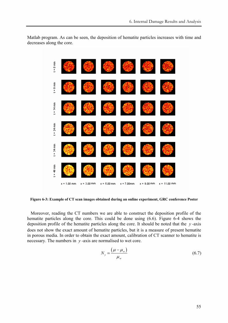
6. Internal Damage Results and Analysis
55
Matlab program. As can be seen, the deposition of hematite particles increases with time and decreases along the core.
Figure 6-3: Example of CT scan images obtained during an online experiment, GRC conference Poster
Moreover, reading the CT numbers we are able to construct the deposition profile of the hematite particles along the core. This could be done using (6.6). Figure 6-4 shows the deposition profile of the hematite particles along the core. It should be noted that the y -axis does not show the exact amount of hematite particles, but it is a measure of present hematite in porous media. In order to obtain the exact amount, calibration of CT scanner to hematite is necessary. The numbers in y -axis are normalised to wet core.
( )wy
w
Nµ µµ−
(6.7)
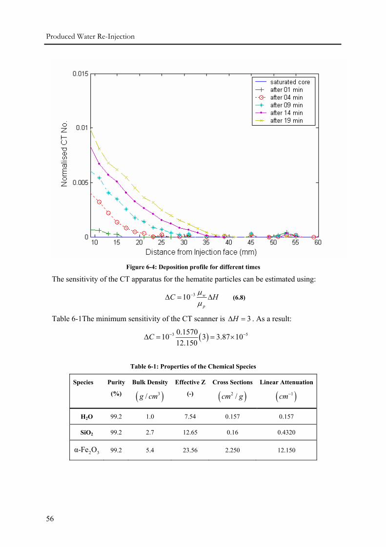
Produced Water Re-Injection
56
Figure 6-4: Deposition profile for different times
The sensitivity of the CT apparatus for the hematite particles can be estimated using:
310 w
p
C Hµµ
−∆ = ∆ (6.8)
Table 6-1The minimum sensitivity of the CT scanner is 3H∆ = . As a result:
( )3 50.157010 3 3.87 1012.150
C − −∆ = = ×
Table 6-1: Properties of the Chemical Species
Species Purity
(%)
Bulk Density
( )3/g cm
Effective Z
(-)
Cross Sections
( )2 /cm g
Linear Attenuation
( )1cm−
H2O 99.2 1.0 7.54 0.157 0.157
SiO2 99.2 2.7 12.65 0.16 0.4320
2 3α-Fe O 99.2 5.4 23.56 2.250 12.150
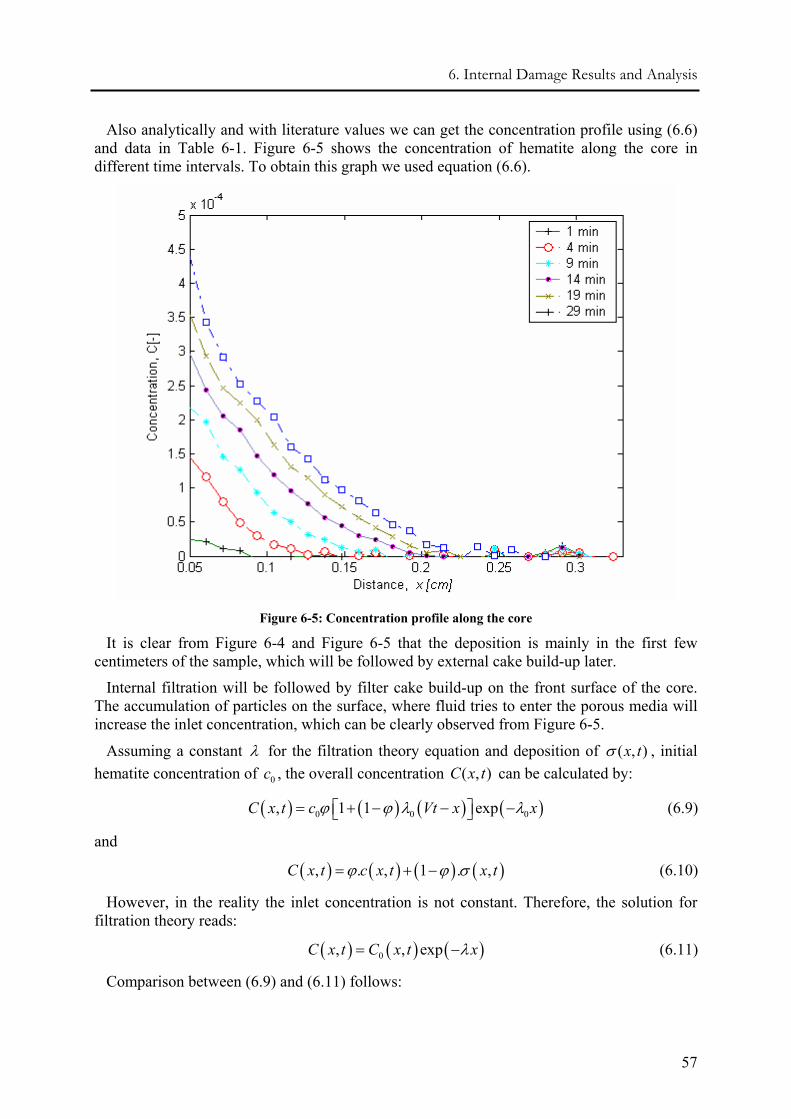
6. Internal Damage Results and Analysis
57
Also analytically and with literature values we can get the concentration profile using (6.6) and data in Table 6-1. Figure 6-5 shows the concentration of hematite along the core in different time intervals. To obtain this graph we used equation (6.6).
Figure 6-5: Concentration profile along the core
It is clear from Figure 6-4 and Figure 6-5 that the deposition is mainly in the first few centimeters of the sample, which will be followed by external cake build-up later.
Internal filtration will be followed by filter cake build-up on the front surface of the core. The accumulation of particles on the surface, where fluid tries to enter the porous media will increase the inlet concentration, which can be clearly observed from Figure 6-5.
Assuming a constant λ for the filtration theory equation and deposition of ( , )x tσ , initial hematite concentration of 0c , the overall concentration ( , )C x t can be calculated by:
( ) ( ) ( ) ( )0 0 0, 1 1 expC x t c Vt x xϕ ϕ λ λ= + − − −⎡ ⎤⎣ ⎦ (6.9)
and
( ) ( ) ( ) ( ), . , 1 . ,C x t c x t x tϕ ϕ σ= + − (6.10)
However, in the reality the inlet concentration is not constant. Therefore, the solution for filtration theory reads:
( ) ( ) ( )0, , expC x t C x t xλ= − (6.11)
Comparison between (6.9) and (6.11) follows:
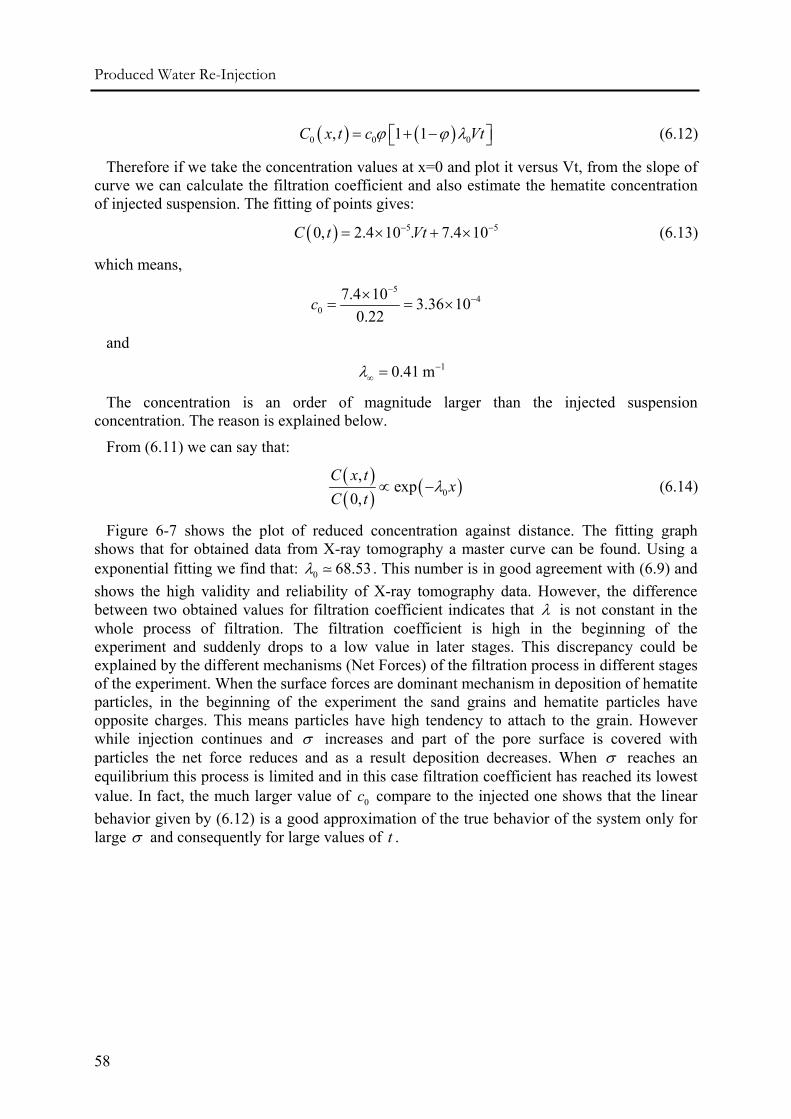
Produced Water Re-Injection
58
( ) ( )0 0 0, 1 1C x t c Vtϕ ϕ λ= + −⎡ ⎤⎣ ⎦ (6.12)
Therefore if we take the concentration values at x=0 and plot it versus Vt, from the slope of curve we can calculate the filtration coefficient and also estimate the hematite concentration of injected suspension. The fitting of points gives:
( ) 5 50, 2.4 10 . 7.4 10C t Vt− −= × + × (6.13)
which means, 5
40
7.4 10 3.36 100.22
c−
−×= = ×
and 10.41 mλ −
∞ =
The concentration is an order of magnitude larger than the injected suspension concentration. The reason is explained below.
From (6.11) we can say that:
( )( ) ( )0
,exp
0,C x t
xC t
λ∝ − (6.14)
Figure 6-7 shows the plot of reduced concentration against distance. The fitting graph shows that for obtained data from X-ray tomography a master curve can be found. Using a exponential fitting we find that: 0 68.53λ . This number is in good agreement with (6.9) and shows the high validity and reliability of X-ray tomography data. However, the difference between two obtained values for filtration coefficient indicates that λ is not constant in the whole process of filtration. The filtration coefficient is high in the beginning of the experiment and suddenly drops to a low value in later stages. This discrepancy could be explained by the different mechanisms (Net Forces) of the filtration process in different stages of the experiment. When the surface forces are dominant mechanism in deposition of hematite particles, in the beginning of the experiment the sand grains and hematite particles have opposite charges. This means particles have high tendency to attach to the grain. However while injection continues and σ increases and part of the pore surface is covered with particles the net force reduces and as a result deposition decreases. When σ reaches an equilibrium this process is limited and in this case filtration coefficient has reached its lowest value. In fact, the much larger value of 0c compare to the injected one shows that the linear behavior given by (6.12) is a good approximation of the true behavior of the system only for large σ and consequently for large values of t .
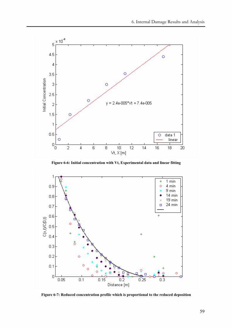
6. Internal Damage Results and Analysis
59
Figure 6-6: Initial concentration with Vt, Experimental data and linear fitting
Figure 6-7: Reduced concentration profile which is proportional to the reduced deposition
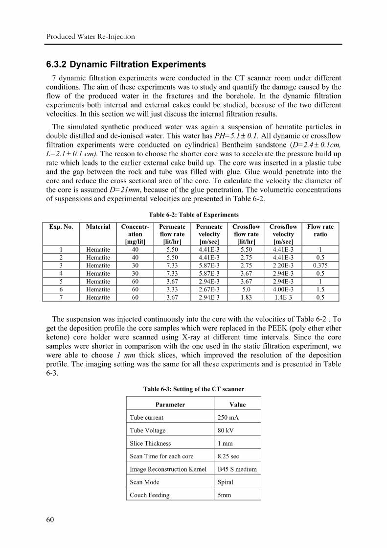
Produced Water Re-Injection
60
6.3.2 Dynamic Filtration Experiments 7 dynamic filtration experiments were conducted in the CT scanner room under different
conditions. The aim of these experiments was to study and quantify the damage caused by the flow of the produced water in the fractures and the borehole. In the dynamic filtration experiments both internal and external cakes could be studied, because of the two different velocities. In this section we will just discuss the internal filtration results.
The simulated synthetic produced water was again a suspension of hematite particles in double distilled and de-ionised water. This water has PH=5.1± 0.1. All dynamic or crossflow filtration experiments were conducted on cylindrical Bentheim sandstone (D=2.4± 0.1cm, L=2.1± 0.1 cm). The reason to choose the shorter core was to accelerate the pressure build up rate which leads to the earlier external cake build up. The core was inserted in a plastic tube and the gap between the rock and tube was filled with glue. Glue would penetrate into the core and reduce the cross sectional area of the core. To calculate the velocity the diameter of the core is assumed D=21mm, because of the glue penetration. The volumetric concentrations of suspensions and experimental velocities are presented in Table 6-2.
Table 6-2: Table of Experiments
Exp. No. Material Concentr-ation
[mg/lit]
Permeate flow rate [lit/hr]
Permeate velocity [m/sec]
Crossflow flow rate [lit/hr]
Crossflow velocity [m/sec]
Flow rate ratio
1 Hematite 40 5.50 4.41E-3 5.50 4.41E-3 1 2 Hematite 40 5.50 4.41E-3 2.75 4.41E-3 0.5 3 Hematite 30 7.33 5.87E-3 2.75 2.20E-3 0.375 4 Hematite 30 7.33 5.87E-3 3.67 2.94E-3 0.5 5 Hematite 60 3.67 2.94E-3 3.67 2.94E-3 1 6 Hematite 60 3.33 2.67E-3 5.0 4.00E-3 1.5 7 Hematite 60 3.67 2.94E-3 1.83 1.4E-3 0.5
The suspension was injected continuously into the core with the velocities of Table 6-2 . To get the deposition profile the core samples which were replaced in the PEEK (poly ether ether ketone) core holder were scanned using X-ray at different time intervals. Since the core samples were shorter in comparison with the one used in the static filtration experiment, we were able to choose 1 mm thick slices, which improved the resolution of the deposition profile. The imaging setting was the same for all these experiments and is presented in Table 6-3.
Table 6-3: Setting of the CT scanner
Parameter Value
Tube current 250 mA
Tube Voltage 80 kV
Slice Thickness 1 mm
Scan Time for each core 8.25 sec
Image Reconstruction Kernel B45 S medium
Scan Mode Spiral
Couch Feeding 5mm
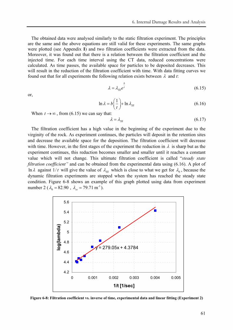
6. Internal Damage Results and Analysis
61
The obtained data were analysed similarly to the static filtration experiment. The principles are the same and the above equations are still valid for these experiments. The same graphs were plotted (see Appendix I) and two filtration coefficients were extracted from the data. Moreover, it was found out that there is a relation between the filtration coefficient and the injected time. For each time interval using the CT data, reduced concentrations were calculated. As time passes, the available space for particles to be deposited decreases. This will result in the reduction of the filtration coefficient with time. With data fitting curves we found out that for all experiments the following relation exists between λ and t:
bt
SSeλ λ= (6.15) or,
1ln ln SSbt
λ λ⎛ ⎞= +⎜ ⎟⎝ ⎠
(6.16)
When t →∞ , from (6.15) we can say that: SSλ λ= (6.17)
The filtration coefficient has a high value in the beginning of the experiment due to the virginity of the rock. As experiment continues, the particles will deposit in the retention sites and decrease the available space for the deposition. The filtration coefficient will decrease with time. However, in the first stages of the experiment the reduction in λ is sharp but as the experiment continues, this reduction becomes smaller and smaller until it reaches a constant value which will not change. This ultimate filtration coefficient is called “steady state filtration coefficient” and can be obtained from the experimental data using (6.16). A plot of lnλ against 1/ t will give the value of SSλ which is close to what we get for 0λ , because the dynamic filtration experiments are stopped when the system has reached the steady state condition. Figure 6-8 shows an example of this graph plotted using data from experiment number 2 ( -1
0 82.90 , 79.71 mssλ λ= = ).
y = 279.05x + 4.3784
4.2
4.4
4.6
4.8
5
5.2
5.4
5.6
0 0.001 0.002 0.003 0.004 0.005
1/t [1/sec]
log(
lam
bda)
Figure 6-8: Filtration coefficient vs. inverse of time, experimental data and linear fitting (Experiment 2)
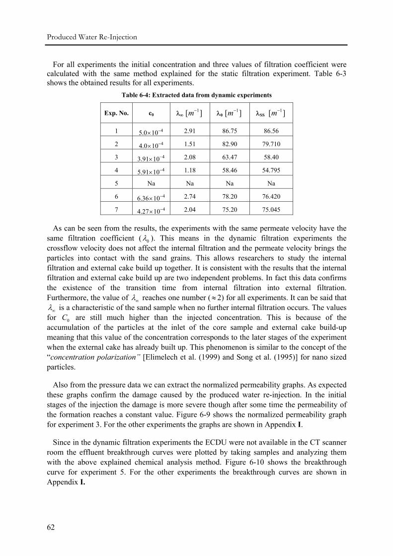
Produced Water Re-Injection
62
For all experiments the initial concentration and three values of filtration coefficient were calculated with the same method explained for the static filtration experiment. Table 6-3 shows the obtained results for all experiments.
Table 6-4: Extracted data from dynamic experiments
Exp. No. c0 λ∞ 1[ ]m− λ0 1[ ]m− λSS 1[ ]m−
1 45.0 10−× 2.91 86.75 86.56
2 44.0 10−× 1.51 82.90 79.710
3 43.91 10−× 2.08 63.47 58.40
4 45.91 10−× 1.18 58.46 54.795
5 Na Na Na Na
6 46.36 10−× 2.74 78.20 76.420
7 44.27 10−× 2.04 75.20 75.045
As can be seen from the results, the experiments with the same permeate velocity have the same filtration coefficient ( 0λ ). This means in the dynamic filtration experiments the crossflow velocity does not affect the internal filtration and the permeate velocity brings the particles into contact with the sand grains. This allows researchers to study the internal filtration and external cake build up together. It is consistent with the results that the internal filtration and external cake build up are two independent problems. In fact this data confirms the existence of the transition time from internal filtration into external filtration. Furthermore, the value of λ∞ reaches one number (≈2) for all experiments. It can be said that λ∞ is a characteristic of the sand sample when no further internal filtration occurs. The values for 0C are still much higher than the injected concentration. This is because of the accumulation of the particles at the inlet of the core sample and external cake build-up meaning that this value of the concentration corresponds to the later stages of the experiment when the external cake has already built up. This phenomenon is similar to the concept of the “concentration polarization” [Elimelech et al. (1999) and Song et al. (1995)] for nano sized particles.
Also from the pressure data we can extract the normalized permeability graphs. As expected these graphs confirm the damage caused by the produced water re-injection. In the initial stages of the injection the damage is more severe though after some time the permeability of the formation reaches a constant value. Figure 6-9 shows the normalized permeability graph for experiment 3. For the other experiments the graphs are shown in Appendix I.
Since in the dynamic filtration experiments the ECDU were not available in the CT scanner room the effluent breakthrough curves were plotted by taking samples and analyzing them with the above explained chemical analysis method. Figure 6-10 shows the breakthrough curve for experiment 5. For the other experiments the breakthrough curves are shown in Appendix I.
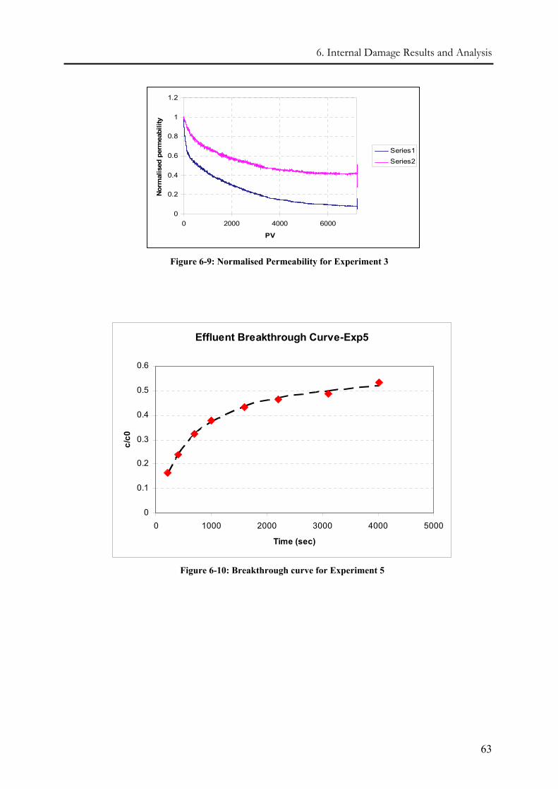
6. Internal Damage Results and Analysis
63
0
0.2
0.4
0.6
0.8
1
1.2
0 2000 4000 6000
PV
Norm
alis
ed p
erm
eabi
lity
Series1Series2
Figure 6-9: Normalised Permeability for Experiment 3
Effluent Breakthrough Curve-Exp5
0
0.1
0.2
0.3
0.4
0.5
0.6
0 1000 2000 3000 4000 5000
Time (sec)
c/c0
Figure 6-10: Breakthrough curve for Experiment 5

Produced Water Re-Injection
64
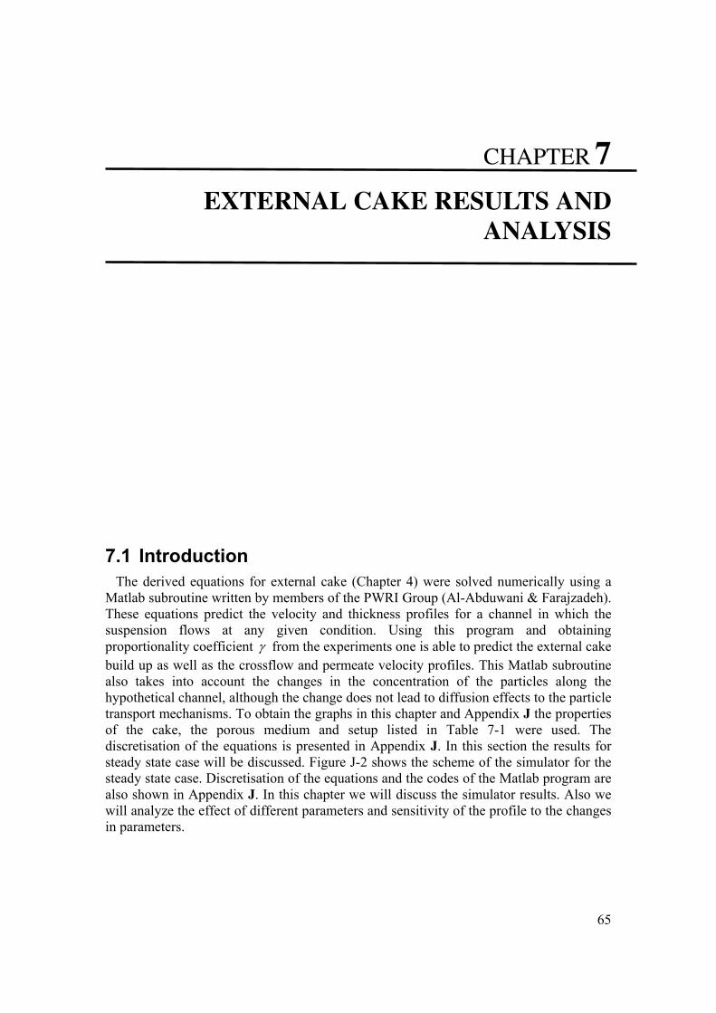
65
CHAPTER 7
7. EXTERNAL CAKE RESULTS AND ANALYSIS
7.1 Introduction The derived equations for external cake (Chapter 4) were solved numerically using a
Matlab subroutine written by members of the PWRI Group (Al-Abduwani & Farajzadeh). These equations predict the velocity and thickness profiles for a channel in which the suspension flows at any given condition. Using this program and obtaining proportionality coefficient γ from the experiments one is able to predict the external cake build up as well as the crossflow and permeate velocity profiles. This Matlab subroutine also takes into account the changes in the concentration of the particles along the hypothetical channel, although the change does not lead to diffusion effects to the particle transport mechanisms. To obtain the graphs in this chapter and Appendix J the properties of the cake, the porous medium and setup listed in Table 7-1 were used. The discretisation of the equations is presented in Appendix J. In this section the results for steady state case will be discussed. Figure J-2 shows the scheme of the simulator for the steady state case. Discretisation of the equations and the codes of the Matlab program are also shown in Appendix J. In this chapter we will discuss the simulator results. Also we will analyze the effect of different parameters and sensitivity of the profile to the changes in parameters.
Produced Water Re-Injection
66
7.2 Simulation Results for Steady State case The permeate flow carries particles toward the porous membrane and they deposit on
its surface. However, contrary to the static filtration the cake growth is not uniform along the channel (green line in Figure 7-1). This is a direct consequence of the shear forces caused by the crossflow velocity which leads to the erosion of the cake. This is the reason why the cake thickness increases along the channel. Since the shear forces decrease, any increase in the cake thickness will result in higher resistance to the permeate velocity to enter the porous medium and therefore, with increasing thickness the permeate velocity decreases along the channel. The growth of the external cake reduces the cross section for crossflow to pass along the channel. Thus, the shear rate at the cake surface increases. These two effects, the permeate flow decrease and the shear rate increase, cause a steady state cake to eventually be reached when the rate of particle convection to the cake surface is balanced by shear back-transport of the particles. Crossflow velocity also decreases with distance from the injection inlet of the channel because of the leak off of the liquid in the channel (permeate flow). The bottom-left graph shows that the volumetric concentration of the particles increases moving toward the end of the channel. The reason is that because of the increase in thickness of the cake, the volume of the cells in the simulated cells decreases for a constant number of particles. The effect of diffusion is neglected due to the high velocities we used. In fact we assume that the only mechanism in transporting of the particles is advection.
Table 7-1: Base case conditions used to run the simulator
Cake Permeability ( ck ) 10.0 µm Porous Medium Perm ( mk ) 1.5 D
Porous Medium thickness ( mL ) 10 cm Back Pressure ( BPP ) 5.0 bar Cake Porosity ( cϕ ) 0.4
Gamma fγ α= 8.33E-3
Setup Length ( L ) 1.0 m Channel Height (H) 5.0 mm Channel Width (W) 20.0 mm Injection rate (Q0) 2.78E-6 m3/sec
Inlet concentration (c0) 40 ppm Particle Radius ( a ) 2.0 µm
Figure 7-2 shows that the pressure decreases slightly along the channel for base case.
However because of the laminar flow the change is not significant and the pressure could be assumed constant. The same story is true for ψ , since it is a direct function of the pressure.
7. External Cake Results and Analysis
67
Figure 7-1: Results from simulator for steady state case
Besides the base case, we ran the simulator for different cases to see the effect of each parameter on the thickness of cake individually. We chose different parameters (particle size, back pressure, porous medium and cake permeability and the proportionality coefficient gamma) by the factors of 0.1, 0.5 and 2 of the base case. For example Figure 7-3 shows the sensitivity of the cake thickness to the size of the particles. This graph shows that as particle radius decreases the thickness of the cake increases. This is quite interesting because it is contrary to what one should see in the static filtration. In static filtration the particles with bigger size will form a higher porosity and thicker cake. In the dynamic or crossflow filtration velocity has two components which insert drag forces on the entering particles. Our model takes into account the drag forces and frictional force. Besides the velocity, according to Stokes law for laminar flow, drag force depends on the radius of the particles. As particle size increases the tangential drag force on the particle increases. This means that the drag force is bigger for the bigger particles. For an open end channel when the drag force overcomes the frictional force the particle will go further or out of the channel but small particles will stay on the surface of the channel and will form the cake. Figures for other parameters are shown in Appendix J and their effect on the cake thickness will be explained in the next section
Produced Water Re-Injection
68
Figure 7-2: Pressure slightly decreases along the channel
Figure 7-3: Sensitivity of the steady state cake thickness to particle size
7. External Cake Results and Analysis
69
7.3 Sensitivity Analysis Figure 7-3 to Figure 7-6 show the sensitivity of the cake thickness to different
parameters at different parts of the cake. We do sensitivity analysis for different parts of the cake because the cake profile is not uniform and to get a feel of the non-linear behavior. All figures indicate that the permeability of the porous medium has no effect on the thickness of the cake because of the assumption of constant permeability for the porous medium. In fact we run the simulator for the external cake without considering the internal filtration. In our analysis the porous medium is just a membrane. Moreover, since the cake has much lower permeability compared to the porous medium the main resistance to the fluid is in the cake itself. The three figures clearly show that the cake thickness has linear relationship with the cake thickness. The thickness of the cake will be changed by the factor that the base cake permeability is multiplied to. It should be noticed that in our modeling the cake permeability is also assumed constant which may not be true in reality.
The cake thickness has also linear relationship with the back pressure. If we double the back pressure, the cake thickness will be doubled and if we reduce the pressure to the half of its initial value, the cake thickness will be half as well. The back pressure is related to the permeate velocity with Darcy’s law. Therefore when the back pressure is higher the permeate velocity is higher which increases the probability of contact of particle with the cake surface. This increases the chance of attachment to the neighborhood particles and will result in higher cake thickness growth.
Figure 7-4: Sensitivity analysis for the first cell
The story of the particle size and Gamma is more complicated. The changes in their values show different effects in different parts of the cake. We chose three sites on the hypothetical channel, the first cell where the fluid enters to the channel, the middle cell and the last. The proportionality coefficient gamma and the particle radius are the
Produced Water Re-Injection
70
parameters that play a significant role in the force balance equations as well as the external cake model equations in Chapter 4. The combinations of these two effects cause the unpredictable effects.
When the magnitude of Gamma is doubled, either the frictional force is doubled or the drag force is halved. In either case, the particle has more chance to be attached to the other particles on the cake surface. But the model doesn’t show the linear relationship between Gamma and the cake thickness. In the first cell when Gamma is doubled the cake thickness increases by the factor of 1.5. But also when Gamma is halved the thickness doubles and when it is reduced to 10% of its initial value the cake becomes much thicker. This nonlinear behavior of the Gamma shows the importance of the Gamma to be measured experimentally for each setup. Without having an idea about the value of the Gamma it is difficult to predict the cake profile along the channel.
Figure 7-5: Sensitivity analysis for the middle cell
Figure 7-6: Sensitivity analysis for the last cell
71
CHAPTER 8
8. CONCLUSIONS AND RECOMMENDATIONS
8.1 Conclusions The following conclusions can be drawn from the results of the experiments of this
work.
• Presence of the solid particles is a potential source of formation damage.
• X-ray computed computer tomography is suitable for extraction of the deposition profile of the particles along the core sample. With this method the actual longitudinal profiles can be obtained in a matter of hours which is much shorter than the other conventional methods. Also the deposition profile can be obtained at different times of the experiments using CT scanner.
• The classical filtration models could predict the extent of the internal damage. The profiles extracted from the experimental data are in a good agreement with the existing filtration theory.
• There is a relation between the filtration coefficient and the injection time. Using X-ray computed tomography the filtration coefficient in different times of the experiment can be obtained. The value of the filtration coefficient in the initial stages of the experiment is quite high due to the availability of more space for particle to be retained. This value drops to a small value at the last stages of the
Produced Water Re-Injection
72
experiment. This value for our core sample was -12 mλ∞ , which can be a property of the Bentheim sand stone.
• In the dynamic or the crossflow experiments the magnitude of the crossflow velocity does not affect the internal filtration. For the experiments with the same permeate velocities and different crossflow velocities the same deposition profile were extracted from the experimental data.
• The results of the experiments confirm the existence of the transition time proposed by Pang and Sharma [1997].
• A novel model for the external cake build up was developed during this project. Using Matlab, a simulator was written which predicts the steady state profiles of the external filter cake.
• The crossflow velocity is the main parameter which affects the erosion of the cake. This can be seen from the calculated C0 for all experiments which has higher valued for higher crossflow velocity.
8.2 Recommendations • In order to study the different stages of the damage and also check the validity of
the transition time experiments with colorful particles are recommended. The possibility of being detected by CT scanner should be checked for selected particles. For colorful latex particles which are not detectable by CT scanner the problem can be solved by coating hematite particles with different colors of the latex, since the hematite particles are detectable using CT scanner.
• In this project the simulated produced water was a suspension of hematite particles. Since the real produced water has another composition for the future experiments the simulated produced water could be selected closer to the reality (for example by adding oil droplet, bacteria…)
• The Bentheim sand stone is homogenous sand with good permeability and porosity which is not the case in most of the reservoirs which suffer for injectivity decline due to produced water re-injection. The experiments can be conducted using other sands.
• To verify the crossflow simulations, experiments should be done on a 1m long set up.
• In the external cake model some simplifying assumptions were made. We ignored the effect of the electrostatic, net gravity and lift forces in our equations. Also the equations were derived for mono-sized particles. For the future work these simplifications can be changed.
8. Conclusions and Recommendations
73
• The transient simulator should be completed to see the pressure build up profiles. This could help to predict the approximate time of the formation fracturing.
• The viscosity of the fluid decreases with increasing temperature. Also temperature changes some properties of the porous medium. Therefore, other experiments can be done in the temperatures above the room temperature. Temperature should also be incorporated in the presented model.
• In order to omit the noises caused by the aluminum plates used in the core holder, a new design is recommended for the core holder.

Produced Water Re-Injection
74
75
REFERENCES [1] Al-Abduwani F.A.H, de Zwart B., Farajzdeh R., van den Broek W.M.G.T and. Currie P.K, (2004a),
”Filtration of Utilising Static Filtration Experiments To Test Existing Filtration Theories For Conformance’”, 2nd Produced Water Workshop, Aberdeen
[2] Al-Abduwani F.A.H, R. Farajzadeh, K. Elewaut, P.K. Currie, W.M.G.T. van den Broek, P.L.J. Zitha, (2004b), “Filtration of Micron-Sized Particles in Granular Media Revealed by X-ray Computed Tomography”, Physical Review letters
[3] Al-Abduwani F.A.H., R.Farajzadeh (2003), “Can Hematite be detected using TA’s CT-scan?”, PWRI Group, TU Delft, Internal Report
[4] Al-Abduwani F.A.H., Shirzadi A., van den Broek W.M.G.T., Currie P.K, (2003), “Formation Damage vs. Solid Particle Deposition profile during Laboratory Simulated PWRI”, SPE 82235
[5] Al-Abduwani F.A.H., R. Farajzadeh, P. Bedrikovetsky, W.M.G.T. van denBroek and P.K. Currie, (2004), “Produced Water Re-injection (PWRI): An Experimental Study Of Internal Filtration And External Filter Cake Build-up”, Poster in Gordon Research conference, 10-16 July, Oxford, UK
[6] Altmann Justus, Siegfrid Ripperger, (1997), “Particle deposition and layer formation at the crossflow microfiltration”, journal of membrane science 124, 119-128
[7] Barkaman, J.H., Davidson, D.H., 1972, ”Measuring water quality and Predicting Well Impairment“, SPE 3543
[8] Bechhold H., (1907), ”Kolloidstuien mit der Filtrationsmethod“, Z.Phys. Chem., 60, 257-318
[9] Bedrikovetsky P., Marchesin D., Shecaira F., Souza A.L., Milanez P.V., Rezende E. (2001), “Characterization of Deep Bed Filtration System from Laboratory Pressure Drop Measurements”, Journal of Petroleum Science and Engineering 32, 167-177
[10] Belfort G., R.H. Davis, A.L. Zydney, (1994), “The behavior of suspensions and macromolcular solutions in crossflow microfiltration”, J. Membrane science 96, 1-58
[11] Davis R.H. and J.D. Sherwood, (1990), “A similarity solution for steady state crossflow microfiltration”, Chem. Eng. Sci., 45, 3204-3209
[12] de Zwart A.H. and Schotting R.J., “Modelling of well clogging”, Delft university of technology, March 2004
[13] Eckstein E.C., P.G. Bailey and A.H. Shapiro, (1977), “Self-diffusion of particles in shear flow of a suspension”, J. Fluid Mech., 79, 191-208
[14] Elimelech Menachen, Albert S. Kim and Subir Bhattacharjee, (1999), “Concentration Polarization of Interacting Solute Particles in Crossflow Membrane Filtration”, Journal of Colloid and Interface Science 212, 81-99
[15] Fitzpatrick, J.A. and L.A. Spielman, (1973), “Filtration of Aqueous Latex Suspensions Through Beds of Glass Spheres”, Journal of Colloid and Interface science, 43, 351-369
[16] Fox Robert W., Alan T.McDonald, (1994), “Introduction to Fluid Mechanics”, section 9, fourth edition
76
[17] Hamaker, H.C. (1937), “The London-van der Waals Attraction Between Spherical Particles”, physica, 4, 1058-1072
[18] Happel, J. (1958), “Viscous flow in multiparticle systems: Slow motions of fluids relative to beds of spherical particle”, AICHE J. 4, 197
[19] Herzig J.P.,. Leclerc D.M. and Le Goff P. (1970) ,”Flow of suspensions through porous media – application to deep filtration”. Industrial and Engineering Chemistry 65 (5), 8-35.
[20] Hofsaess, T. and Kleintz, W. (2003), “30 Years of Predicting Injectivity After Barkman and Davidson: Where are we today?”, SPE 82231
[21] Hunter R.J., (1987), “Foundations of Colloid Science”, Oxford Univ. Press, New York, 1987, chap 7, pp 168-227
[22] Ison, C.R. and K.J. Ives, (1969), “Removal Mechanism in Deep Bed Filtration”, Chem. Eng. Sci., 24, 717-729
[23] Ives, K.J., (11967), “Deep filters”, Filtr sep. (March, April), 125-135
[24] Iwasaki T., (1937), “Some Notes on Sand Filtration”, J. Am. Water Works Ass. 29, 1591-1602
[25] Jackson, J.D. (1975), “Classical electrodynamics”, 2nd ed., Wiley N.Y.
[26] Jiao D and M. Sharma, (1994), “Mechanism of Cake Buildup in Crossflow Filtration of Colloidal Suspensions”, Journal of Colloid and Interface Science 162, 454-462
[27] Jiamhong Ren, Aaron I. Packman, Claire Welty, (2001), “Analysis of an observed relationship between colloid collision efficiency and mean collector grain size”, Colloid and surface science
[28] Jonathan Wills, M.A (2000), “A Survey of Offshore Oilfield Drilling Wastes and Disposal Techniques to Reduce the Ecological Impact of Sea Dumping”, Sakhalin Environment watch
[29] Khatib, Z., and P.Verbeek, 2003, “Water to Value-Produce water Management for Sustainable Field Development of mature and Green Fields”, Journal of Petroleum Technology, January, pp. 26-28.
[30] Kuhnen, F., K.Barmettler, S. Bhattacharjee, M. Elimelech, and R. Kretzschmar, (2000) J. colloid and Interface Science, 231, 32-41
[31] Mackley M.R. and N.E. Sherman, (1992), “Cross-flow Cake Filtration Mechanisms and Kinetics”, Chemical Engineering Science, Vol. 47, No. 12, 3067-3084
[32] Marchesin D., Hime G., Bedrikovetsky P., S.Souza A.L., Alvarez A. and Siqueira A.G., “Analytical Formulas in Formation Damage Under Linear and Radial Geometry, Derivation and Numerical Evaluation” , ver 1.5
[33] McDowell-Boyer Laura M., Hunt James R. and Sitar N., (1986), “Particle Transport through Porous Media”, Water Resources Research, Vol. 22, No. 13, 1901-1921
[34] Mendez Zuleyka Del Carmen, Ph.D , (1999) “Flow of Dilute Oil-in-Water Emulsions in Porous Media”, The University of Texas at Austin
[35] Ochi J., Detienne J.L, Rivet P.and Lacourie Y., (1999) “External Filter Cake Properties during Injection of Produced Waters.” SPE 54773
77
[36] Ochi J., Detienne J.L, Rivet P.and Lacourie Y., (1999) “External Filter Cake Properties during Injection of Produced Waters.” SPE 54773
[37] Pang, S. (1996) “colloid retention and flow in porous media”, phd dissertation, the university of Texas at Austin
[38] Pang S. and Sharma M.M. (1994), “A Model for Predicting Injectivity Decline in Water Injection Well”. SPE 28489
[39] Rochon, J., M.R. Creusot, P. Rivet, C. Roque and M. Renard, (1996), “Water Quality for Injection Wells”, SPE 31122
[40] Rubin G., (1977), ”Widrestands und Auftriebsbeiwerte von ruhenden kugelformigen Partikeln in stationaren, wandahen laminaren Grenzschichten“, Dissertation, TH Karlsruhe
[41] Song Lianfa and Menachem Elimelech, (1995), “Theory of Concentration Polarization in crossflow Filtration”, J. Chem. Soc. Faraday Trans., 91(19), 3389-3398
[42] Sharma, M.M., Pang, S., Wennberg, K.E., Morgenthaler, L.N., (2000), Injectivity decline in water-injection wells: an offshore Gulf of Mexico case study, SPE Prod. & Facilities 15 (1), Feb. 2000
[43] Schluep Thomas and fritz Widmer, (1996), “Initial Transient Effects during Crossflow Microfiltration of yeast Suspension”, Journal of Membrane Science, 115, 113-145
[44] Tent V.A. and K.T. Nijenhuis, (1992), “Turbidity study of the process of film formation of polymer particles in drying thin films of acrylic lattice”, J. Colloid and interface science, 150, 97-114
[45] Tien C. and Payatakes A.C. (1979), “Advances in Deep Bed Filtration.” AIChE Journal 25 (5), 737-759.
[46] Tien C., Bai R.and Ramarao B.V. (1997),” Analysis of Cake Growth in Cake Filtration: Effect of Fine Particle Retention”. AIChE 43 (1) 33-44
[47] Veil John A., (2004), “An Overview of Produced Water in the United States”, 2nd Produced Water Workshop
[48] Wennberg, K.E, Sharma, M.M, “Determination of the Filtration Coefficient and the Transition Time for Water Injection Wells”, SPE 38181

78
79
NOMENCLATURE
tS : skin factor µ : viscosity
injP : injection pressure q : flow rate k : permeability η : total collision probability
Iη : collision probability due to interception
Dη : collision probability due to diffusion
imη : collision probability due to impaction
sη : collision probability due to sedimentation
Eη : collision probability due to surface forces
pd : particle diameter
gd : grain diameter ϕ : effective porosity
pρ : particle density
fρ : fluid density ,U u : Darcy’s velocity
g : gravity acceleration
Bk : Boltzman constant (=1023) T: absolute temperature A: Hamaker constant
pv : particle velocity
( ),c x t : volumetric concentrations of the suspended particles
( ),x tσ : volumetric concentrations of the deposited particles
0k : absolute permeability ( )k σ : Formation Damage coefficient (relative permeability) :λ Filtration coefficient
L: length of the porous media t : time
0c : initial concentration of suspended particles xXL
= : scaled length
UtTLϕ
= : scaled time
80
0
cCc
= : scaled concentration of the suspended particles
0
Scσϕ
= : scaled concentration of the deposited particles
Λ : scaled filtration coefficient 0λ : initial filtration coefficient λ∞ : final filtration coefficient
0Λ : scaled initial filtration coefficient
FV : clogging front velocity
cα : clean-bed collision efficiency Φ : hydraulic head 0i : clean bed gradient
K: hydraulic conductivity Rσ : resistance due to deposition I: injectivity index j : inverse of injectivity index J : non-dimensional impedance *t : transition time
n: number of particles attached to one grain ga : cross-sectional area of a grain
DF : drag force
DC : drag coefficient τ : shear force
LF : lift force
BF : buoyancy force
GF : net gravity force
eF : electrostatic force
fF : frictional force
vdWF : van der Waals force
NF : sum of Normal forces ψ : Stern potential
0ε : absolute permittivity of the free space
rε : dielectric constant of the fluid κ : reciprocal of the thickness double layer ξ : zeta potential
wτ : wall shear stress
0µ : permeate viscosity
wΦ : particle volume fraction at the filter surface
81
bΦ : particle volume fraction in the bulk
0,BoD : Brownian diffusion coefficient f : Coulombs frictional coefficient γ : proportionality coeffiecient

82
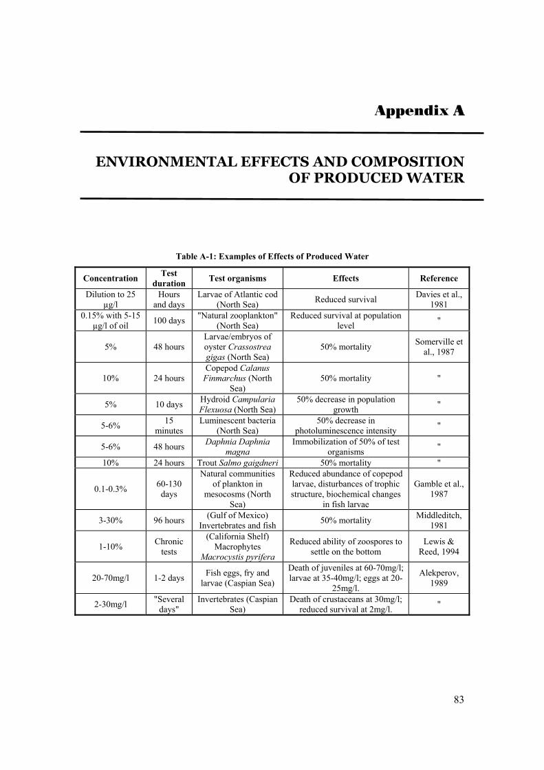
83
Appendix A
ENVIRONMENTAL EFFECTS AND COMPOSITION
OF PRODUCED WATER
Table A-1: Examples of Effects of Produced Water
Concentration Test duration Test organisms Effects Reference
Dilution to 25 µg/l
Hours and days
Larvae of Atlantic cod (North Sea) Reduced survival Davies et al.,
1981 0.15% with 5-15
µg/l of oil 100 days "Natural zooplankton" (North Sea)
Reduced survival at population level "
5% 48 hours Larvae/embryos of oyster Crassostrea gigas (North Sea)
50% mortality Somerville et al., 1987
10% 24 hours Copepod Calanus
Finmarchus (North Sea)
50% mortality "
5% 10 days Hydroid Campularia Flexuosa (North Sea)
50% decrease in population growth "
5-6% 15 minutes
Luminescent bacteria (North Sea)
50% decrease in photoluminescence intensity "
5-6% 48 hours Daphnia Daphnia magna
Immobilization of 50% of test organisms "
10% 24 hours Trout Salmo gaigdneri 50% mortality "
0.1-0.3% 60-130 days
Natural communities of plankton in
mesocosms (North Sea)
Reduced abundance of copepod larvae, disturbances of trophic structure, biochemical changes
in fish larvae
Gamble et al., 1987
3-30% 96 hours (Gulf of Mexico) Invertebrates and fish 50% mortality Middleditch,
1981
1-10% Chronic tests
(California Shelf) Macrophytes
Macrocystis pyrifera Reduced ability of zoospores to
settle on the bottom Lewis &
Reed, 1994
20-70mg/l 1-2 days Fish eggs, fry and larvae (Caspian Sea)
Death of juveniles at 60-70mg/l; larvae at 35-40mg/l; eggs at 20-
25mg/l. Alekperov,
1989
2-30mg/l "Several days"
Invertebrates (Caspian Sea)
Death of crustaceans at 30mg/l; reduced survival at 2mg/l. "
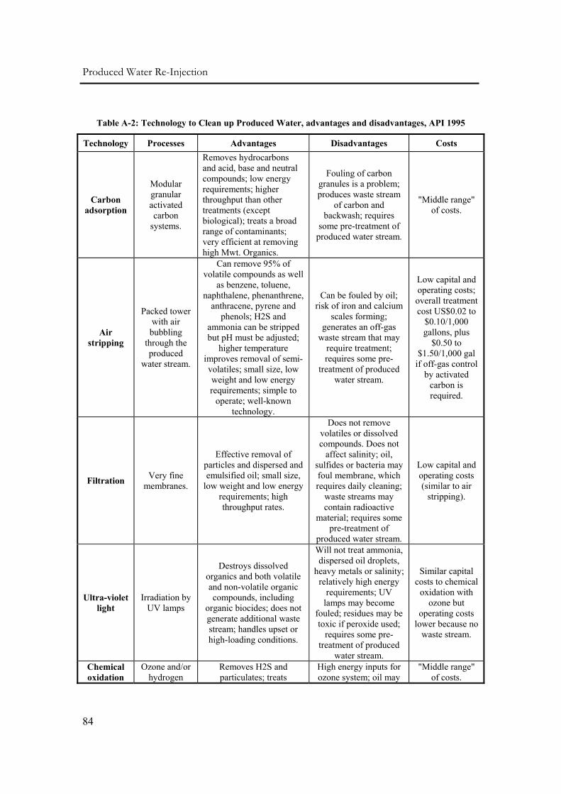
Produced Water Re-Injection
84
Table A-2: Technology to Clean up Produced Water, advantages and disadvantages, API 1995
Technology Processes Advantages Disadvantages Costs
Carbon adsorption
Modular granular activated carbon
systems.
Removes hydrocarbons and acid, base and neutral compounds; low energy requirements; higher throughput than other treatments (except biological); treats a broad range of contaminants; very efficient at removing high Mwt. Organics.
Fouling of carbon granules is a problem; produces waste stream
of carbon and backwash; requires
some pre-treatment of produced water stream.
"Middle range" of costs.
Air stripping
Packed tower with air bubbling
through the produced
water stream.
Can remove 95% of volatile compounds as well
as benzene, toluene, naphthalene, phenanthrene,
anthracene, pyrene and phenols; H2S and
ammonia can be stripped but pH must be adjusted;
higher temperature improves removal of semi-volatiles; small size, low weight and low energy requirements; simple to
operate; well-known technology.
Can be fouled by oil; risk of iron and calcium
scales forming; generates an off-gas
waste stream that may require treatment; requires some pre-
treatment of produced water stream.
Low capital and operating costs; overall treatment cost US$0.02 to
$0.10/1,000 gallons, plus
$0.50 to $1.50/1,000 gal
if off-gas control by activated
carbon is required.
Filtration Very fine membranes.
Effective removal of particles and dispersed and emulsified oil; small size,
low weight and low energy requirements; high throughput rates.
Does not remove volatiles or dissolved compounds. Does not
affect salinity; oil, sulfides or bacteria may foul membrane, which requires daily cleaning;
waste streams may contain radioactive
material; requires some pre-treatment of
produced water stream.
Low capital and operating costs (similar to air
stripping).
Ultra-violet light
Irradiation by UV lamps
Destroys dissolved organics and both volatile and non-volatile organic compounds, including
organic biocides; does not generate additional waste stream; handles upset or high-loading conditions.
Will not treat ammonia, dispersed oil droplets,
heavy metals or salinity; relatively high energy
requirements; UV lamps may become
fouled; residues may be toxic if peroxide used;
requires some pre-treatment of produced
water stream.
Similar capital costs to chemical
oxidation with ozone but
operating costs lower because no
waste stream.
Chemical oxidation
Ozone and/or hydrogen
Removes H2S and particulates; treats
High energy inputs for ozone system; oil may
"Middle range" of costs.
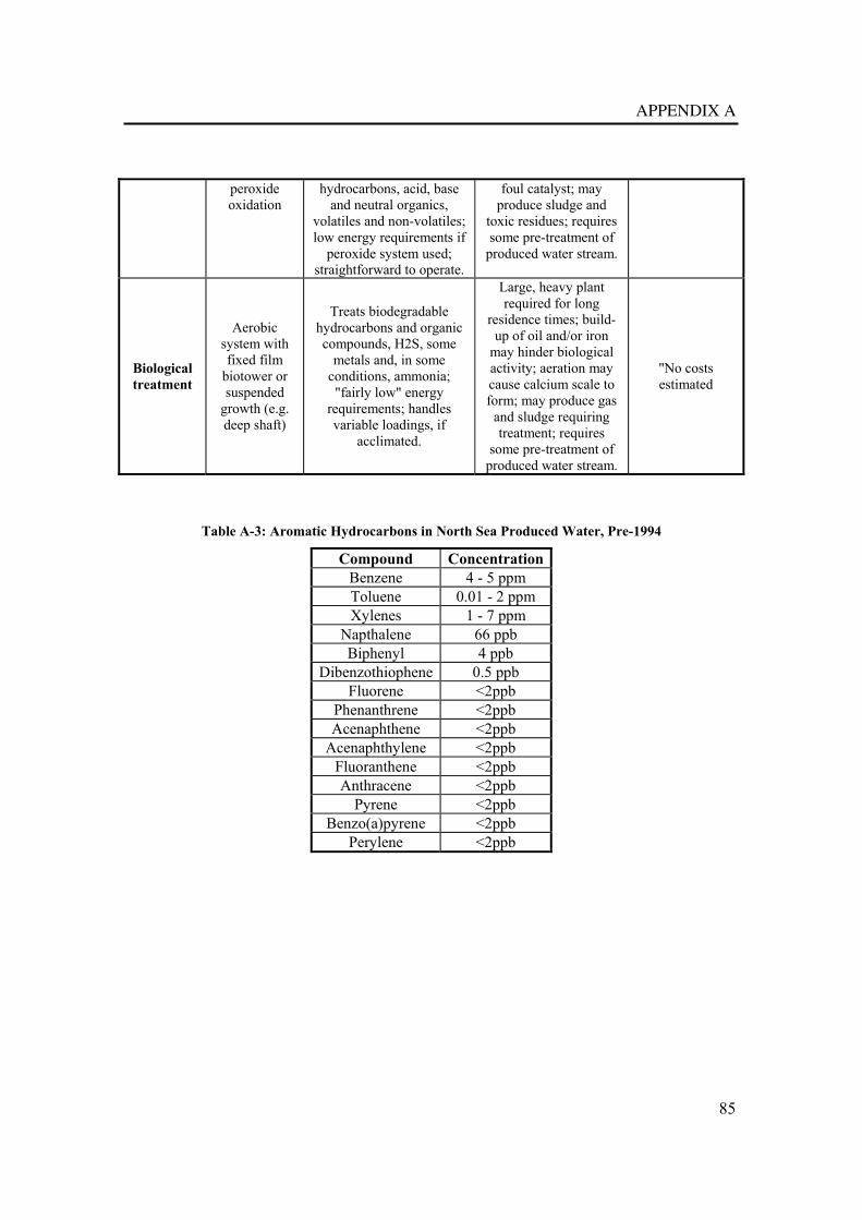
APPENDIX A
85
peroxide oxidation
hydrocarbons, acid, base and neutral organics,
volatiles and non-volatiles; low energy requirements if
peroxide system used; straightforward to operate.
foul catalyst; may produce sludge and
toxic residues; requires some pre-treatment of
produced water stream.
Biological treatment
Aerobic system with fixed film
biotower or suspended
growth (e.g. deep shaft)
Treats biodegradable hydrocarbons and organic compounds, H2S, some
metals and, in some conditions, ammonia; "fairly low" energy
requirements; handles variable loadings, if
acclimated.
Large, heavy plant required for long
residence times; build-up of oil and/or iron
may hinder biological activity; aeration may cause calcium scale to form; may produce gas
and sludge requiring treatment; requires
some pre-treatment of produced water stream.
"No costs estimated
Table A-3: Aromatic Hydrocarbons in North Sea Produced Water, Pre-1994
Compound ConcentrationBenzene 4 - 5 ppm Toluene 0.01 - 2 ppm Xylenes 1 - 7 ppm
Napthalene 66 ppb Biphenyl 4 ppb
Dibenzothiophene 0.5 ppb Fluorene <2ppb
Phenanthrene <2ppb Acenaphthene <2ppb
Acenaphthylene <2ppb Fluoranthene <2ppb Anthracene <2ppb
Pyrene <2ppb Benzo(a)pyrene <2ppb
Perylene <2ppb
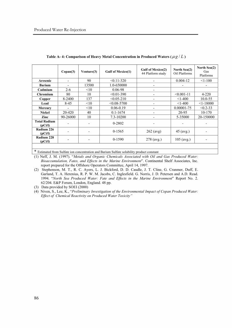
Produced Water Re-Injection
86
Table A- 4: Comparison of Heavy Metal Concentration in Produced Waters ( /g Lµ )
(1) Neff, J. M. (1997). “Metals and Organic Chemicals Associated with Oil and Gas Produced Water: Bioaccumulation, Fates, and Effects in the Marine Environment”. Continental Shelf Associates, Inc. report prepared for the Offshore Operators Committee, April 14, 1997.
(2) Stephenson, M. T., R. C. Ayers, L. J. Bickford, D. D. Caudle, J. T. Cline, G. Cranmer, Duff, E. Garland, T. A. Herenius, R. P. W. M. Jacobs, C. Inglesfield. G. Norris, J. D. Petersen and A.D. Read. 1994. “North Sea Produced Water: Fate and Effects in the Marine Environment” Report No. 2. 62/204. E&P Forum, London, England. 48 pp.
(3) Data provided by SOEI (2000) (4) Niven, S., Lee, K., “Preliminary Investigation of the Environmental Impact of Copan Produced Water:
Effect of Chemical Reactivity on Produced Water Toxicity”
Copan(3) Venture(3) Gulf of Mexico(1) Gulf of Mexico(2) 44 Platform study
North Sea(2) Oil Platforms
North Sea(2) Gas
Platforms Aresenic - 90 <0.11-320 - 0.004-12 <1-100 Barium - 13500 1.0-650000 - - -
Cadmium 2-6 <10 0.06-98 - Chromium 80 10 <0.01-390 - <0.001-11 4-220
Copper 8-2400 137 <0.05-210 - <1-400 10.0-55 Lead 8-45 <10 <0.08-5700 - <1-400 <1-18000
Mercury - <10 0.06-0.19 - 0.00001-75 <0.2-33 Nickel 20-420 40 0.1-1674 - 20-95 10-170 Zinc 90-26000 10 7.3-10200 - 5-35000 20-150000
Total Radium (pCi/l) - - 0-2802 - - -
Radium 226 (pCi/l) - - 0-1565 262 (avg) 45 (avg.) -
Radium 228 (pCi/l) - - 0-1590 278 (avg.) 105 (avg.) -
* Estimated from Sulfate ion concentration and Barium Sulfate solubility product constant
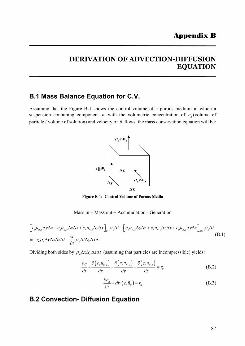
87
Appendix B
DERIVATION OF ADVECTION-DIFFUSION
EQUATION
B.1 Mass Balance Equation for C.V.
Assuming that the Figure B-1 shows the control volume of a porous medium in which a suspension containing component n with the volumetric concentration of nc (volume of particle / volume of solution) and velocity of u flows, the mass conservation equation will be:
Figure B-1: Control Volume of Porous Media
Mass in – Mass out = Accumulation - Generation
, , , , , ,n n x n n y n n z n n n x n n y n n z nin out
n n n
c u y z c u z x c n y x t c u y z c u z x c u y x t
cr y x z t t y x zt
ρ ρ
ρ ρ
⎡ ⎤ ⎡ ⎤∆ ∆ + ∆ ∆ + ∆ ∆ ∆ − ∆ ∆ + ∆ ∆ + ∆ ∆ ∆⎣ ⎦ ⎣ ⎦∂
= − ∆ ∆ ∆ ∆ + ∆ ∆ ∆ ∆∂
(B.1)
Dividing both sides by n x y z tρ ∆ ∆ ∆ ∆ (assuming that particles are incompressible) yields:
( ) ( ) ( ),, ,n n yn n x n n z
n
c uc u c uc rt x y z
∂∂ ∂∂+ + + =
∂ ∂ ∂ ∂ (B.2)
( )nn n n
c div c u rt
∂+ =
∂ (B.3)
B.2 Convection- Diffusion Equation
ρn xc.u
ρn yc.u
ρn zc.u
∆y∆x
∆z
Produced Water Re-Injection
88
In a binary system of just one solute and one solvent, the diffusion flux of the solute is defined as:
ncu c= −J u (B.4)
Then, (B.3) becomes:
( )nn n
c div c div rt
∂+ + =
∂Ju (B.5)
Using Fick’s law we have:
( )( )gradnn n n
c div c D c rt
∂+ − =
∂u (B.6)
Finally according to the filtration theory for the rate of deposition in the porous media we can write:
n nr ctσ λ∂
= − = −∂
u (B.7)
Substituting (B.7) into (B.6) yields:
( )( )grad 0nn n
c div c D ct t
σ∂ ∂+ − + =
∂ ∂u (B.8)
Writing (B.8) in the x direction considering the porosity of the porous media:
( ) ( ) 2
2 0n xc cu cDt x xσ∂ + ∂ ∂
+ − =∂ ∂ ∂
(B.9)
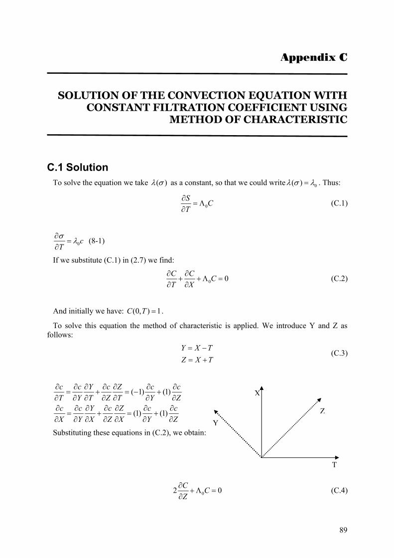
89
Appendix C
SOLUTION OF THE CONVECTION EQUATION WITH
CONSTANT FILTRATION COEFFICIENT USING METHOD OF CHARACTERISTIC
C.1 Solution To solve the equation we take ( )λ σ as a constant, so that we could write 0( )λ σ λ= . Thus:
0S CT
∂= Λ
∂ (C.1)
0cTσ λ∂
=∂
(8-1)
If we substitute (C.1) in (2.7) we find:
0 0C C CT X
∂ ∂+ + Λ =
∂ ∂ (C.2)
And initially we have: (0, ) 1C T = .
To solve this equation the method of characteristic is applied. We introduce Y and Z as follows:
Y X TZ X T
= −= +
(C.3)
( 1) (1)
(1) (1)
c c Y c Z c cT Y T Z T Y Zc c Y c Z c cX Y X Z X Y Z
∂ ∂ ∂ ∂ ∂ ∂ ∂= + = − +
∂ ∂ ∂ ∂ ∂ ∂ ∂∂ ∂ ∂ ∂ ∂ ∂ ∂
= + = +∂ ∂ ∂ ∂ ∂ ∂ ∂
Substituting these equations in (C.2), we obtain:
02 0C CZ
∂+ Λ =
∂ (C.4)
X
T
YZ

Produced Water Re-Injection
90
The solution for (C.4) is:
01ln ( )2
C Z g Y= − Λ + (C.5)
and if we replace Y and Z in (C.5) , using (C.3) the final solution is:
01ln ( ) ( )2
C X T g X T= − Λ + + − (C.6)
with C(0,T)=1
to determine ( )g X T− we use the initial condition:
0
0
1ln(1) ( ) ( )2
1 ( ) ( )2
T g T
T g T
λ
λ
= − + −
− − = −
Then
01( ) ( )2
g X T X T− = − Λ − (C.7)
And if we put (C.7) in (C.6) we will get:
0 XC e−Λ= (C.8)
Figure 1 clearly shows that the solution is in the area X T≥ .
C.2 Second method
0 0C C CT X
∂ ∂+ + Λ =
∂ ∂
0C C CT X
∂ ∂+ =−Λ∂ ∂
and we have: (0, ) 1C T =
1=dsdT )(1 rcsT +=⇒ with T(r,0)=r rrc =⇒ )(1 rsT +=⇒ (C.9)
1=dsdX )(2 rcsX +=⇒ with X(r,0)=0 0)(2 =⇒ rc sX =⇒ (C.10)
0dz zds=−Λ 0 3ln ( )z s c r⇒ =−Λ + with z(r,0)=1 0)(3 =⇒ rc 0ln z s⇒ =−Λ
Then we can simply write: 0( , ) ( ( , ), ( , ) sc X T z r X T s X T e−Λ= = and since we have X=s then we would have:
0 XC e−Λ=
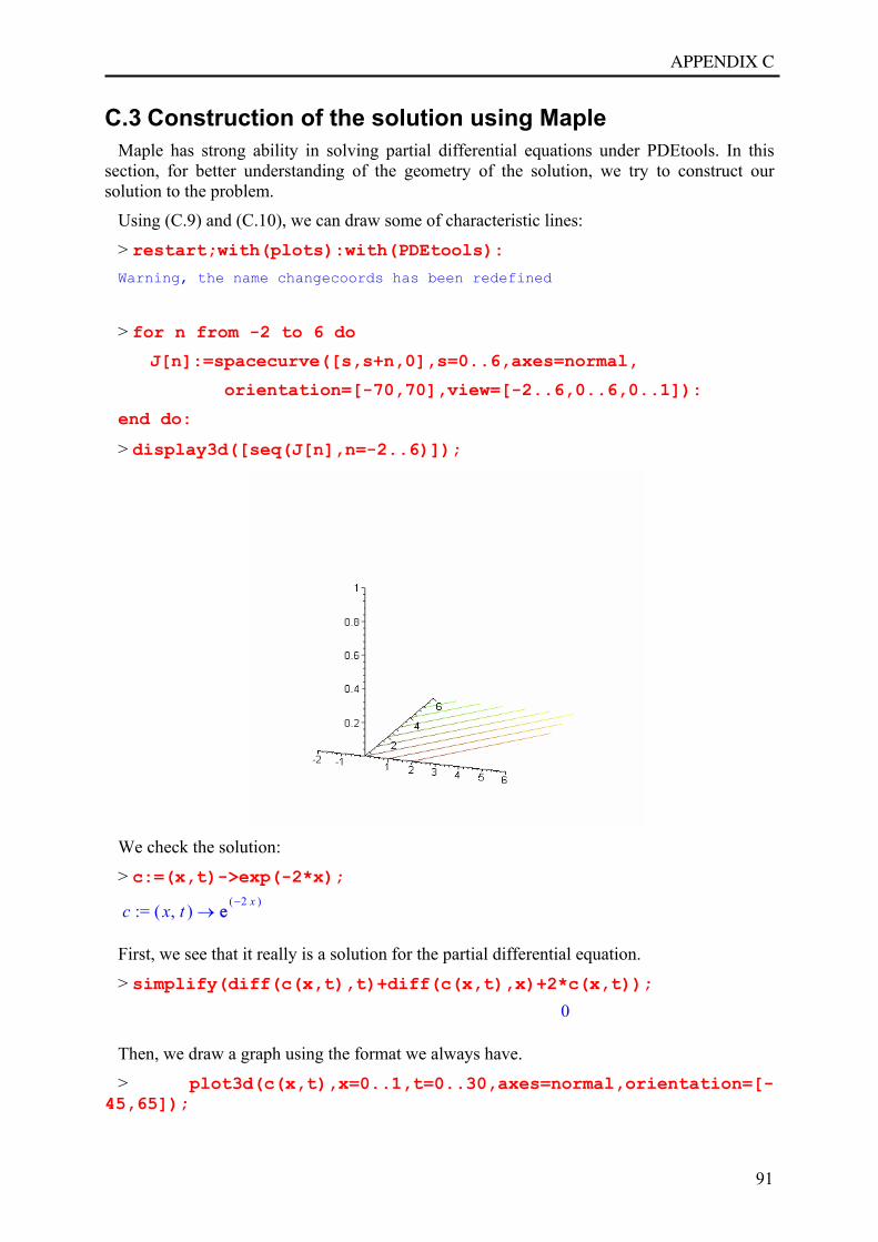
APPENDIX C
91
C.3 Construction of the solution using Maple Maple has strong ability in solving partial differential equations under PDEtools. In this
section, for better understanding of the geometry of the solution, we try to construct our solution to the problem.
Using (C.9) and (C.10), we can draw some of characteristic lines:
> restart;with(plots):with(PDEtools): Warning, the name changecoords has been redefined
> for n from -2 to 6 do J[n]:=spacecurve([s,s+n,0],s=0..6,axes=normal,
orientation=[-70,70],view=[-2..6,0..6,0..1]):
end do:
> display3d([seq(J[n],n=-2..6)]);
We check the solution:
> c:=(x,t)->exp(-2*x);
:= c → ( ),x t e( )−2 x
First, we see that it really is a solution for the partial differential equation.
> simplify(diff(c(x,t),t)+diff(c(x,t),x)+2*c(x,t));
0
Then, we draw a graph using the format we always have.
> plot3d(c(x,t),x=0..1,t=0..30,axes=normal,orientation=[-45,65]);
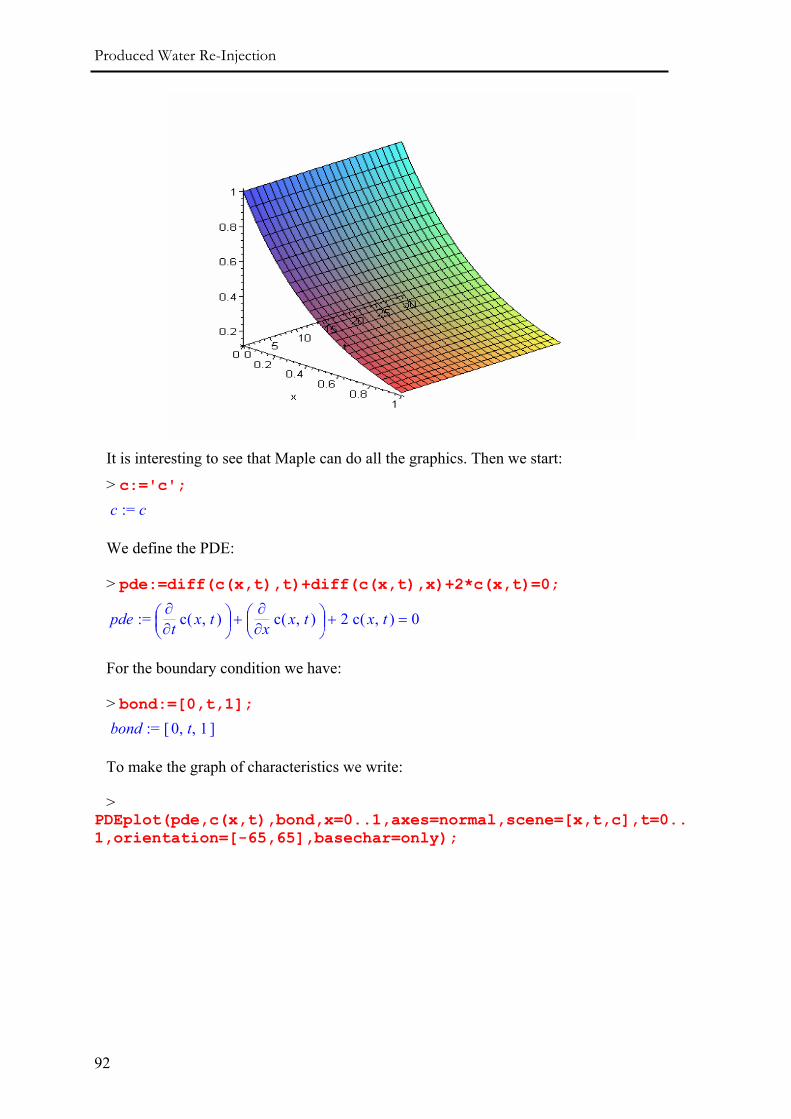
Produced Water Re-Injection
92
It is interesting to see that Maple can do all the graphics. Then we start:
> c:='c'; := c c
We define the PDE:
> pde:=diff(c(x,t),t)+diff(c(x,t),x)+2*c(x,t)=0;
:= pde = + + ⎛⎝⎜⎜
⎞⎠⎟⎟∂
∂t ( )c ,x t ⎛
⎝⎜⎜
⎞⎠⎟⎟∂
∂x ( )c ,x t 2 ( )c ,x t 0
For the boundary condition we have:
> bond:=[0,t,1]; := bond [ ], ,0 t 1
To make the graph of characteristics we write:
> PDEplot(pde,c(x,t),bond,x=0..1,axes=normal,scene=[x,t,c],t=0..1,orientation=[-65,65],basechar=only);
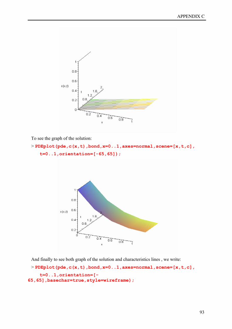
APPENDIX C
93
To see the graph of the solution:
> PDEplot(pde,c(x,t),bond,x=0..1,axes=normal,scene=[x,t,c], t=0..1,orientation=[-65,65]);
And finally to see both graph of the solution and characteristics lines , we write:
> PDEplot(pde,c(x,t),bond,x=0..1,axes=normal,scene=[x,t,c], t=0..1,orientation=[-
65,65],basechar=true,style=wireframe);
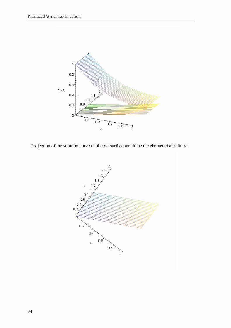
Produced Water Re-Injection
94
Projection of the solution curve on the x-t surface would be the characteristics lines:
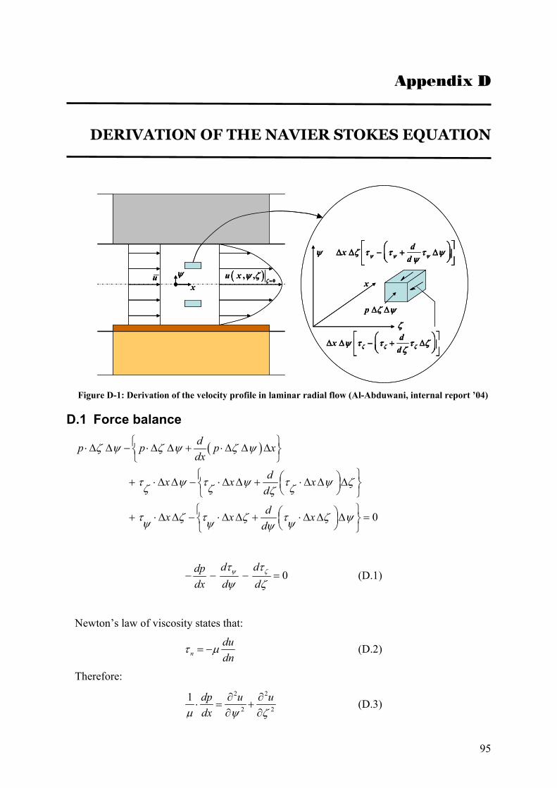
95
Appendix D
DERIVATION OF THE NAVIER STOKES EQUATION
xψu ( )
0, ,u x
ζψ ζ
=
ζ
ψ
x
p ζ ψ∆ ∆
dxdψ ψ ψζ τ τ τ ψψ
⎡ ⎤⎛ ⎞∆ ∆ − + ∆⎢ ⎥⎜ ⎟⎝ ⎠⎣ ⎦
dxdζ ζ ζψ τ τ τ ζζ
⎡ ⎤⎛ ⎞∆ ∆ − + ∆⎢ ⎥⎜ ⎟⎝ ⎠⎣ ⎦
xψu ( )
0, ,u x
ζψ ζ
=
ζ
ψ
x
p ζ ψ∆ ∆
dxdψ ψ ψζ τ τ τ ψψ
⎡ ⎤⎛ ⎞∆ ∆ − + ∆⎢ ⎥⎜ ⎟⎝ ⎠⎣ ⎦
dxdζ ζ ζψ τ τ τ ζζ
⎡ ⎤⎛ ⎞∆ ∆ − + ∆⎢ ⎥⎜ ⎟⎝ ⎠⎣ ⎦
Figure D-1: Derivation of the velocity profile in laminar radial flow (Al-Abduwani, internal report ’04)
D.1 Force balance
( )
0
dp p p xdx
dx x xd
dx x xd
ζ ψ ζ ψ ζ ψ
τ ψ τ ψ τ ψ ζζ ζ ζζ
τ ζ τ ζ τ ζ ψψ ψ ψψ
⎧ ⎫⋅∆ ∆ − ⋅∆ ∆ + ⋅∆ ∆ ∆⎨ ⎬⎩ ⎭
⎧ ⎫⎛ ⎞+ ⋅∆ ∆ − ⋅∆ ∆ + ⋅∆ ∆ ∆⎜ ⎟⎨ ⎬⎝ ⎠⎩ ⎭
⎧ ⎫⎛ ⎞+ ⋅∆ ∆ − ⋅∆ ∆ + ⋅∆ ∆ ∆ =⎜ ⎟⎨ ⎬⎝ ⎠⎩ ⎭
0d ddp
dx d dψ ζτ τψ ζ
− − − = (D.1)
Newton’s law of viscosity states that:
ndudn
τ µ= − (D.2)
Therefore: 2 2
2 2
1 dp u udxµ ψ ζ
∂ ∂⋅ = +
∂ ∂ (D.3)
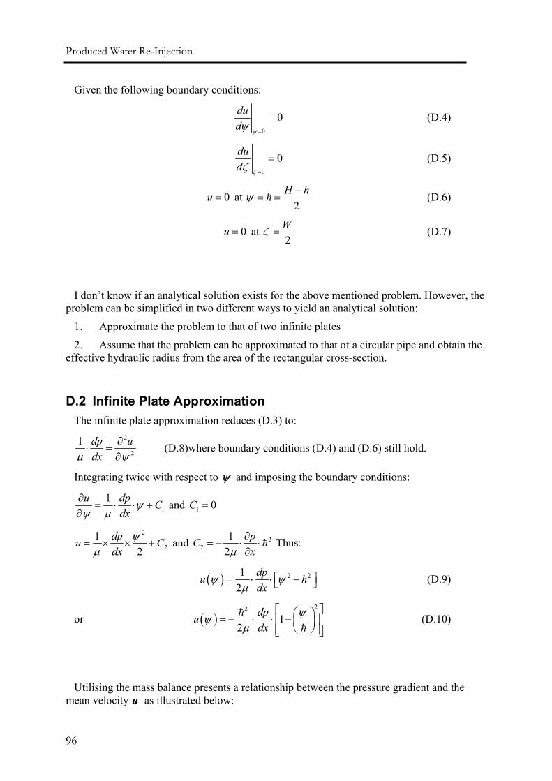
Produced Water Re-Injection
96
Given the following boundary conditions:
0
0dud ψψ =
= (D.4)
0
0dud ζζ =
= (D.5)
0u = at 2
H hψ −= = (D.6)
0u = at 2
Wζ = (D.7)
I don’t know if an analytical solution exists for the above mentioned problem. However, the problem can be simplified in two different ways to yield an analytical solution:
1. Approximate the problem to that of two infinite plates
2. Assume that the problem can be approximated to that of a circular pipe and obtain the effective hydraulic radius from the area of the rectangular cross-section.
D.2 Infinite Plate Approximation The infinite plate approximation reduces (D.3) to:
2
2
1 dp udxµ ψ
∂⋅ =
∂ (D.8)where boundary conditions (D.4) and (D.6) still hold.
Integrating twice with respect to ψ and imposing the boundary conditions:
11u dp C
dxψ
ψ µ∂
= ⋅ ⋅ +∂
and 1 0C =
2
21
2dpu Cdx
ψµ
= × × + and 22
12
pCxµ∂
= − ⋅ ⋅∂
Thus:
( ) 2 212
dpudx
ψ ψµ
⎡ ⎤= ⋅ ⋅ −⎣ ⎦ (D.9)
or ( )22
12
dpudx
ψψµ
⎡ ⎤⎛ ⎞= − ⋅ ⋅ −⎢ ⎥⎜ ⎟⎝ ⎠⎢ ⎥⎣ ⎦
(D.10)
Utilising the mass balance presents a relationship between the pressure gradient and the mean velocity u as illustrated below:

APPENDIX D
97
( )0
2 2u W W u dρ ρ ψ ψ⋅ = ⋅ ∫ (D.11)which yields:
( )2 2
0
12 dpu ddx
ψ ψµ
= ⋅ −∫
3
2
0
123
dpudx
ψψµ
⎡ ⎤= − ⋅ −⎢ ⎥
⎣ ⎦
and thus, 2
3dp udx
µ= − (D.12)
Combining equations (D.10) and (D.12) yields:
( ) 2 22
32
uu ψ ψ⎡ ⎤= ⋅ ⋅ −⎣ ⎦ (D.13)
or ( )23 1
2u u ψψ
⎡ ⎤⎛ ⎞= ⋅ ⋅ −⎢ ⎥⎜ ⎟⎝ ⎠⎢ ⎥⎣ ⎦
Given that:
( ) dpdxψτ ψ ψ= − ⋅
the shear stress at a given position ψ is:
( ) 2
3 uψ
µτ ψ ψ= ⋅ (D.14)
And the shear stress at the wall:
,3
wu
ψ ψ
µτ τ=
= = (D.15)
or ,6
wu
H hψ ψ
µτ τ=
= =−
D.3 Equivalent Circular Tube Approximation Equating the cross-sectional area to that of an equivalent circle yields the following:
( )2hR W H hπ = ⋅ −
Produced Water Re-Injection
98
2h
WRπ
= (D.16)where hR is the equivalent hydraulic radius.
Using the equations derived for radial flow, we have:
2
4h
h
u rRµτ = ⋅ (D.17)
which is in terms of the measured dimensions:
2h
u rWπ µτ = ⋅ (D.18)
The shear stress at the wall is given by:
4w
h
uRµτ = (D.19)
which is in terms of the measured dimensions:
42w u
Wπτ µ= ⋅ (D.20)
D.4 Comparison between the two approaches The shear stress at the cake surface csτ was obtained using two methods:
1. Infinite plate assumption yields:
3cs
uψ
µτ τ=
= =
2. Effective circular tube assumption yields:
42cs u
Wπτ µ= ⋅
It can be seen that the results obtained using the two different approaches yield; ( )1
cs cs hτ τ −= and ( )1/ 2cs cs hτ τ −= respectively.
The results obtained using the two infinite plate approximation will be used.
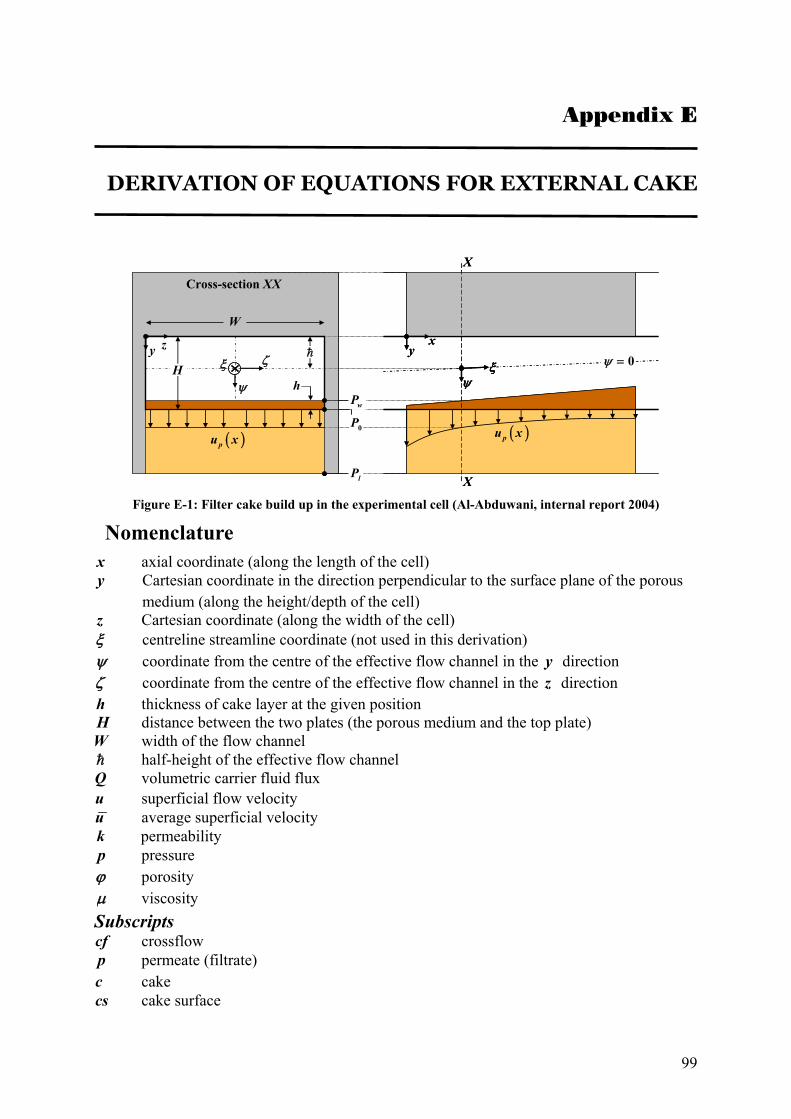
99
Appendix E
DERIVATION OF EQUATIONS FOR EXTERNAL CAKE
xy
X
X
ψψ
ζξ 0ψ =ξ
W
hH
( )pu x( )pu x
zy
Cross-section XX
wP
0P
lP
xy
X
X
ψψ
ζξ 0ψ =ξ
WW
hH
( )pu x( )pu x
zy
Cross-section XX
wP
0P
lP Figure E-1: Filter cake build up in the experimental cell (Al-Abduwani, internal report 2004)
Nomenclature x axial coordinate (along the length of the cell) y Cartesian coordinate in the direction perpendicular to the surface plane of the porous
medium (along the height/depth of the cell) z Cartesian coordinate (along the width of the cell) ξ centreline streamline coordinate (not used in this derivation) ψ coordinate from the centre of the effective flow channel in the y direction ζ coordinate from the centre of the effective flow channel in the z direction h thickness of cake layer at the given position H distance between the two plates (the porous medium and the top plate) W width of the flow channel
half-height of the effective flow channel Q volumetric carrier fluid flux u superficial flow velocity u average superficial velocity k permeability p pressure ϕ porosity µ viscosity Subscripts cf crossflow p permeate (filtrate) c cake cs cake surface
Produced Water Re-Injection
100
pm porous medium w pressure in the wellbore at a given cross-section, which also the pressure acting on the
cake surface for the same cross-section. 0 pressure at the interface between the porous medium and the filter cake l location l , which is the radius of drainage of the given well
E.1 Force Balance As was mentioned in chapter (?), various forces act on a particle in colloidal system. These
forces are:
• Normal (Permeate) Drag Force ( rF )
• Tangential (Crossflow) Drag Force ( dF )
• Lift Forces ( LF )
• Electrostatic Forces ( eF ) and Particle interaction
• Diffusion
• Friction Force ( fF )
• Net Gravity Force ( GF )
E.1.1 Tangential Drag Force The tangential drag force can be calculated by one of three ways:
Poiseuille’s Law For Infinite Plate d w sF Aτ= (E.1)
24d w aF a
ψπ τ
= −= (E.2)
Using Navier-Stokes derivation in Appendix (?):
2
3 cfuµτ ψ=
aψ = − , thus:
( )22
34 cf
d
uF a a
µπ= −
212 1cf
d
u aF aµ
π ⎛ ⎞= −⎜ ⎟⎝ ⎠
(E.3)
Radius of particle is very small compare to half height of the channel; therefore the tangential drag force can be approximated as:
212 cfd
uF a
µπ≈ (E.4)
APPENDIX E
101
224( )
cfd
uF a
H hµ
π≈−
(E.5)
Poiseuille’s Law for Equivalent Tube
24h a
d w r rF aπ τ
== (E.6)
2
4 cfh
h
ur
Rµ
τ = (E.7)
where ( )h
W H hR
π−
= and ( )a
W H h ar
π− −
=
Thus,
( )
( )4a
cfr
W H h au
W H hπτ µ
π− −
= ⋅ ⋅−
(E.8)
( ) ( )
4 1a
cfr
auW H h H h
πτ µ⎡ ⎤
= ⋅ ⋅ −⎢ ⎥− −⎢ ⎥⎣ ⎦
(E.9)
4 12 2a
cfr
auWπτ µ
⎡ ⎤= ⋅ ⋅ −⎢ ⎥
⎣ ⎦
42a
cfru
Wπτ µ≈ ⋅ (E.10)
And therefore:
24 42D cfF a uWππ µ≈ ⋅ ⋅ (E.11)
Or
( )
216D cfF a uW H h
ππ µ≈ ⋅ ⋅−
(E.12)
Stoke’s law For laminar flow with very small Reynolds number, stoke’s law for drag forces yields:
6Stoke cf aF au
ψπ µ
= −= (E.13)
From Appendix (?) we have:
( ) 2 2
2
32
cfcf
uu ψ ψ⎡ ⎤= ⋅ ⋅ −⎣ ⎦
(E.14)
By setting aψ = − :
Produced Water Re-Injection
102
( ) ( )222
32
cfcf
uu a a⎡ ⎤− = ⋅ ⋅ − −⎣ ⎦ (E.15)
( ) 22
3 22
cfcf
uu a a a⎡ ⎤− = ⋅ ⋅ −⎣ ⎦ (E.16)
( )2
32
cfcf
u au a a⎡ ⎤
− = ⋅ ⋅ −⎢ ⎥⎣ ⎦
(E.17)
( )3 cf
cf
u au a− ≈ (E.18)
And therefore,
218 cf
d
uF a
µπ≈ ⋅ (E.19)
General Form of the Tangential Drag Force From above mentioned equations a general form can be proposed for tangential drag force
which can be written in the form of:
2
2cf
d
uF a
µα π= (E.20)
( )
2 cfd
uF a
H hµ
α π=−
(E.21)
E.1.2 Normal Drag Force The normal drag force acts on a particle due to permeate velocity and can be calculated
using Stoke’s law:
6r pF auπµ=
E.1.3 Electrostatic Forces According to DLVO theory there are two main electrostatic forces acting on a particle:
double layer forces and Van der Waals forces.
E.1.4 Frictional Force Friction force is the Coulomb frictional force, which is proportional to the normal forces
acting on the particle.
.f NF f F=
Here f is the Coulomb friction coefficient.
E.2 Solving for the Force Balance Inequality During a crossflow filtration process particle will be deposited if friction force overcomes
the tangential drag force. Therefore, while the tangential force overcomes the friction force, cake reaches its critical or equilibrium thickness and forces satisfy the inequality:
APPENDIX E
103
( )D e r GF f F F F≥ + + (E.22)
Using the above mentioned equations:
( ) ( )2 6cf
e p G
ua f F au F
H hµ
απ πµ= + +−
(E.23)
Case A: Both Electrostatic and Net Gravity forces are negligible
( ) ( )2 6cf
p
ua f au
H hµ
απ πµ=−
(E.24)
( )6cf
p
u H hu a
γ −= (E.25)
Where,
fγα
= (E.26)
Case B: Net Gravity Force is not negligible but Electrostatic Forces are negligible
( )
2 3463
cfp
ua f au a g
R hµ
α π πµ π ρ⎛ ⎞= + ∆⎜ ⎟− ⎝ ⎠ (E.27)
( )( )1 2cf pu u H hγ γ= + − (E.28)
Where, 16 f
aγ
α= and 2
43a gργµα∆
= .
Case C: Electrostatic and net Gravity Forces are not negligible
E.3 Derivation of Equations at Steady State Condition Before we go to complicated cases, we start with steady state equations, which means filter
cake has reached its critical height and no deposition occurs.
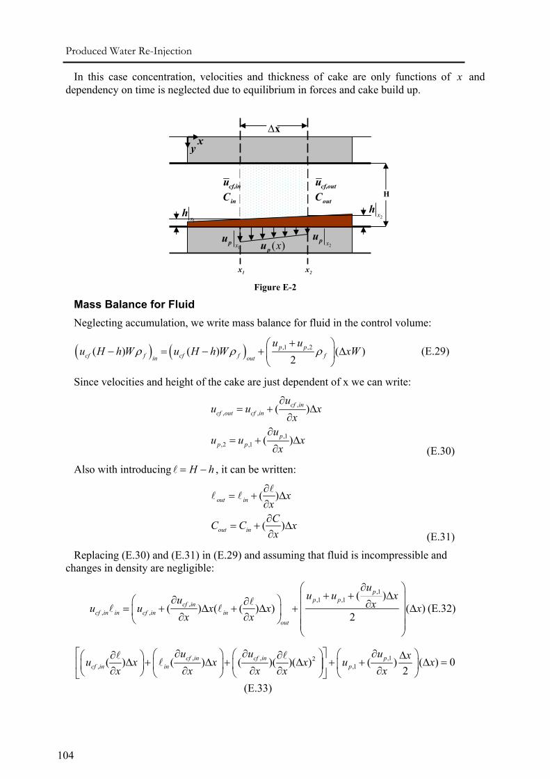
Produced Water Re-Injection
104
In this case concentration, velocities and thickness of cake are only functions of x and dependency on time is neglected due to equilibrium in forces and cake build up.
Figure E-2
Mass Balance for Fluid Neglecting accumulation, we write mass balance for fluid in the control volume:
( ) ( ) ,1 ,2( ) ( ) ( )2
p pcf f cf f fin out
u uu H h W u H h W xWρ ρ ρ
+⎛ ⎞− = − + ∆⎜ ⎟
⎝ ⎠ (E.29)
Since velocities and height of the cake are just dependent of x we can write:
,, ,
,1,2 ,1
( )
( )
cf incf out cf in
pp p
uu u x
xu
u u xx
∂= + ∆
∂∂
= + ∆∂ (E.30)
Also with introducing H h= − , it can be written:
( )
( )
out in
out in
xxCC C xx
∂= + ∆
∂∂
= + ∆∂ (E.31)
Replacing (E.30) and (E.31) in (E.29) and assuming that fluid is incompressible and changes in density are negligible:
,1,1 ,1
,, ,
( )( ) ( ( ) ) ( )
2
pp p
cf incf in in cf in in
out
uu u xu xu u x x x
x x
∂⎛ ⎞+ + ∆⎜ ⎟∂⎛ ⎞∂ ∂= + ∆ + ∆ + ∆⎜ ⎟⎜ ⎟∂ ∂ ⎜ ⎟⎝ ⎠ ⎜ ⎟
⎝ ⎠
(E.32)
, , ,12, ,1( ) ( ) ( )( )( ) ( ) ( ) 0
2cf in cf in p
cf in in p
u u u xu x x x u xx x x x x
⎡ ∂ ∂ ⎤ ∂⎛ ⎞ ⎛ ⎞ ⎛ ⎞∂ ∂ ∆⎛ ⎞∆ + ∆ + ∆ + + ∆ =⎢ ⎥⎜ ⎟ ⎜ ⎟ ⎜ ⎟⎜ ⎟∂ ∂ ∂ ∂ ∂⎝ ⎠ ⎝ ⎠ ⎝ ⎠ ⎝ ⎠⎣ ⎦ (E.33)
H
∆xx
y
cf,inuinC
cf,outuoutC
1x 2x
( )xpu
1xh 2x
h
1xpu
2xpu
APPENDIX E
105
Dividing by x∆ :
, , ,1, ,1( ) ( ) ( )( )( ) ( ) 0
2cf in cf in p
cf in in p
u u u xu x ux x x x x
⎡ ∂ ∂ ⎤ ∂⎛ ⎞ ⎛ ⎞ ⎛ ⎞∂ ∂ ∆⎛ ⎞ + + ∆ + + =⎢ ⎥⎜ ⎟ ⎜ ⎟ ⎜ ⎟⎜ ⎟∂ ∂ ∂ ∂ ∂⎝ ⎠ ⎝ ⎠ ⎝ ⎠ ⎝ ⎠⎣ ⎦ (E.34)
When 0x∆ → third and fourth terms are negligible:
,, ,1( ) ( ) 0cf in
cf in in p
uu u
x x⎡ ∂ ⎤⎛ ⎞∂⎛ ⎞ + + =⎢ ⎥⎜ ⎟⎜ ⎟∂ ∂⎝ ⎠ ⎝ ⎠⎣ ⎦
(E.35)
( )cf
p
uu
x∂
= −∂
(E.36)
And finally we can write:
( )( )cfp
u H hu
x∂ −
= −∂
(E.37)
Mass Balance Equation for Particles
( ) ( ) ,1 ,2 ,1 ,2 ( ( ) )( ) ( ) ( )
2 2p p p p p p
cf p cf p pin out
c c u u c H h xWu c H h W u c H h W xW
tρ
ρ ρ ρ⎡ + + ⎤ ∂ − ∆⎛ ⎞
− − − + ∆ =⎢ ⎥⎜ ⎟ ∂⎝ ⎠⎣ ⎦ (E.38)
For steady state case the right side term of (E.38) is zero. Assuming that particles are incompressible and using (E.30) and (E.31):
,,
,1,,1 ,2 ,1 ,2
( ) ( ) ( )
0( ) ( )( )
2 2
cf incf in in in
pcf in in inp p p p
u Cu x C x xx x x
uCu C C C x u u xx x x
⎡ ⎤⎛ ∂ ⎞⎛ ⎞ ∂ ∂⎛ ⎞⎛ ⎞+ ∆ + ∆ + ∆⎢ ⎥⎜ ⎟⎜ ⎟⎜ ⎟⎜ ⎟∂ ∂ ∂⎝ ⎠⎝ ⎠⎝ ⎠⎢ ⎥⎝ ⎠⎢ ⎥∂⎛ ⎞∂− =⎢ ⎥+ + ∆ + + ∆⎜ ⎟⎢ ⎥∂ ∂+ ∆⎜ ⎟⎢ ⎥⎜ ⎟⎢ ⎥⎜ ⎟
⎝ ⎠⎣ ⎦
(E.39)
Dividing by x∆ and putting 0x∆ → :
,, , ,1 ,1( ) ( ) ( ) 0cf in
cf in in cf in in in in p p
uCu C u C C ux x x
⎡ ∂ ⎤⎛ ⎞∂ ∂⎛ ⎞ ⎛ ⎞+ + + =⎢ ⎥⎜ ⎟⎜ ⎟ ⎜ ⎟∂ ∂ ∂⎝ ⎠ ⎝ ⎠ ⎝ ⎠⎣ ⎦ (E.40)
,, , ,1 ,1( ) ( ) ( ) 0cf in
in cf in in cf in in p p
u CC u u C ux x x
⎡ ∂ ⎤⎛ ⎞∂ ∂⎛ ⎞+ + + =⎢ ⎥⎜ ⎟ ⎜ ⎟∂ ∂ ∂⎝ ⎠⎝ ⎠⎣ ⎦ (E.41)
( )
( ) 0cfcf p p
u CC u C ux x
⎛ ⎞∂ ∂⎛ ⎞⎜ ⎟ + + =⎜ ⎟⎜ ⎟∂ ∂⎝ ⎠⎝ ⎠ (E.42)
Using (E.36):
( ) 0p cf p p
CCu u C ux
∂⎛ ⎞− + + =⎜ ⎟∂⎝ ⎠ (E.43)
Produced Water Re-Injection
106
In steady state 0pC = , because the number of particles getting deposited and being removed from cake are identical.
( ) 0p cfCCu ux
∂⎛ ⎞− + =⎜ ⎟∂⎝ ⎠
( )( ) 0cf pCu H h u Cx
∂− − =
∂
( )
( ) ( )( ) ( )
p
cf
C x u xCx u x H h x
∂=
∂ − (E.44)
Using (E.25), we will come up with:
( )2( ) 6 ( )
dC a dxC x H h x
=−
(E.45)
( )20 6 ( )( )x a dx
H h xC x Ae −∫= (E.46)
Here A is the integration constant.
Derivation of Equations for Thickness of the Cake (E.37) states that the flux along the experimental setup decreases due to the leakoff of the
permeate flux.
pQ Wux
∂= −
∂ (E.47)
( )( ) ( ). . ( )cfQ x u x W H h x= − (E.48)
Permeate velocity can be quantified using Darcy’s law and measuring the pressure decline in y direction:
ip
k puyµ∂
=∂
(E.49)
Here, ik is the permeability of the medium and µ viscosity of the fluid carrying the particles. Then for the filter cake it can be written as:
( ) pw o
c
u hp p
kµ
− = (E.50)
And for the porous medium within the drainage length:
( ) po l
u lp p
kµ
− = (E.51)
Adding (E.50) to (E.51):
( )w l pc
h lp p uk k
µ⎛ ⎞
− = +⎜ ⎟⎝ ⎠
(E.52)
From (E.52) another equation can be written for permeate velocity as:
APPENDIX E
107
( ) 1w l
pc
p p h luk kµ
−− ⎛ ⎞
= +⎜ ⎟⎝ ⎠
(E.53)
(E.53) can be re-arranged as:
( )w l cp
c
p p k kukh k lµ
− ⎛ ⎞= ⎜ ⎟+⎝ ⎠
(E.54)
With introducing
ck lk
Θ = (E.55)
and
( )c w lk p pψ
µ−
= (E.56)
Permeate velocity can be written as:
puhψ
=+Θ
(E.57)
As can be seen from (E.57), permeate velocity, pu , is a function of thickness of the external filter cake:
( )( )p pu u h x=
Putting (E.48) and (E.57) into(E.25):
6 ( )( )Q
H hW H ha
h
γψ
−− =
+Θ
(E.58)
Then we can find for Q: 26 ( )W H hQ
a hγ ψ −
=+Θ
(E.59)
If we re-arrange it:
( ) ( )
( )
22
2
( ) 2 ( )6
d dh dhH h H h h H hdQ dx dx dxWdx a h
ψ ψ ψγ
⎛ ⎞⎡ ⎤− − − +Θ − −⎜ ⎟⎢ ⎥⎣ ⎦⎜ ⎟=⎜ ⎟+Θ⎜ ⎟⎝ ⎠
(E.60)
Equating (E.47) and (E.60):
6 ( )( ) ( ) 2d H h dhH h H ha dx h dxγ ψψ ψ⎡ − ⎤⎛ ⎞− = − − − +⎜ ⎟⎢ ⎥+Θ⎝ ⎠⎣ ⎦
(E.61)
Produced Water Re-Injection
108
6 ( ) ( )1 ( ) 2H h d H h dhH ha dx h dxγ ψ
ψ⎡ ⎤− −⎛ ⎞− = − − +⎜ ⎟⎢ ⎥+Θ⎝ ⎠⎣ ⎦
(E.62)
6 ( )( ) 2 1H h dh H h dH ha h dx dxγ ψ
ψ⎡ ⎤− −⎛ ⎞− + − − =⎜ ⎟⎢ ⎥+Θ⎝ ⎠⎣ ⎦ 0
(E.63)
From Error! Reference source not found.:
( )2
12 cfudpdx H h
µ= −
− (E.64)
Replacing (E.25) and (E.57) into (E.64) we get:
( )( )
72dpdx a H h h
γµψ= −
− +Θ (E.65)
from (E.65) and (E.56) it can be followed that:
( )( )
721 ckddx a H h h
γψψ
= −− +Θ
(E.66)
Therefore, (E.63) will change to:
( )726 ( ) 2 1ckH h dhH h
a h dx a hγγ ⎡ ⎤−⎛ ⎞− + + − =⎢ ⎥⎜ ⎟+Θ +Θ⎝ ⎠⎣ ⎦
(E.67)
Or:
( ) ( )
722 6
ckdh h adx H h H h a h
γγ
⎡ ⎤+Θ⎡ ⎤= −⎢ ⎥⎢ ⎥+ Θ+ − +Θ⎣ ⎦ ⎣ ⎦ (E.68)
Using (E.25) and (E.57), (E.68) becomes:
722
p c
cf p
u kdh hdx h H u a u
γ ψ⎡ ⎤+Θ⎡ ⎤= −⎢ ⎥⎢ ⎥+ Θ+⎣ ⎦ ⎢ ⎥⎣ ⎦ (E.69)
Calculation of cake thickness in the right boundary Combining (E.25) and (E.57) yields:
( )6.cf
H hu
a hγ ψ−
=+Θ
(E.70)
Putting (E.70) in (E.48) follows:
( )26 WQ H ha hγ ψ
= −+Θ
(E.71)
If we solve (E.71) for h we will get:
( )( )24
12
Qa Qa Qa W Hh H
W
γ ψ
γ ψ
± + +Θ= + (E.72)
(E.72) gives the thickness of cake for given flow rates. This equation can be used to calculate the thickness in the right boundary.
APPENDIX E
109
E.4 Derivation of Equations for Transient Case (No Erosion) Mass Balance Equation for fluid in suspension
( )( ) ( )( ) ( ) ( )( ),1 ,2
2f cp p
cf f cf f fin out
H h xWu uu H h W u H h W xW
tρ ϕ
ρ ρ ρ∂ − ∆+⎛ ⎞
− = − + ∆ +⎜ ⎟ ∂⎝ ⎠ (E.73)
Assuming that fluid is incompressible and repeating the same procedure as we did for
steady state case, we will get the following equation:
( )( ) ( )cf
p c
u H h H hu
x tϕ
∂ − ∂ −− = +
∂ ∂ (E.74)
Mass Balance Equation for Particles
( )( ) ( )( )
( ) ( )( ),1 ,2 ,1 ,2
2 2
cf p cf pin out
pp p p pp
u C H h W u C H h W
H h xWu u C CxW
t
ρ ρ
ρρ
− − − =
∂ − ∆+ +⎛ ⎞∆ +⎜ ⎟ ∂⎝ ⎠
(E.75)
Assuming that particles are incompressible and all number of deposited and entering particles into the system are identical we will end up with:
( )( ) ( )cf
p
u C H h C H hu C
x t∂ − ∂ −⎡ ⎤⎣ ⎦− = +
∂ ∂ (E.76)
Or:
( ) ( ) ( ) ( )p cf p
H h H hC CC u H h u u C C H ht x t t
∂ − ∂ −⎛ ⎞ ∂ ∂+ + − + = − − −⎜ ⎟∂ ∂ ∂ ∂⎝ ⎠
( )( ) ( ) ( )cf
cf p
H h u H hC CC H h u u C C H hx x t t
⎡ ⎤∂ − ∂ −∂ ∂⎣ ⎦ + − + = − − −∂ ∂ ∂ ∂
(E.77)
Putting (E.74) into (E.77) gives:
( ) ( ) ( ) ( )p cf p
H h H hC CC u H h u u C C H ht x t t
∂ − ∂ −⎛ ⎞ ∂ ∂− + + − + = − − −⎜ ⎟∂ ∂ ∂ ∂⎝ ⎠
(E.78)
With simplifying (E.78) we will get:
0cfC Cux t
∂ ∂+ =
∂ ∂ (E.79)
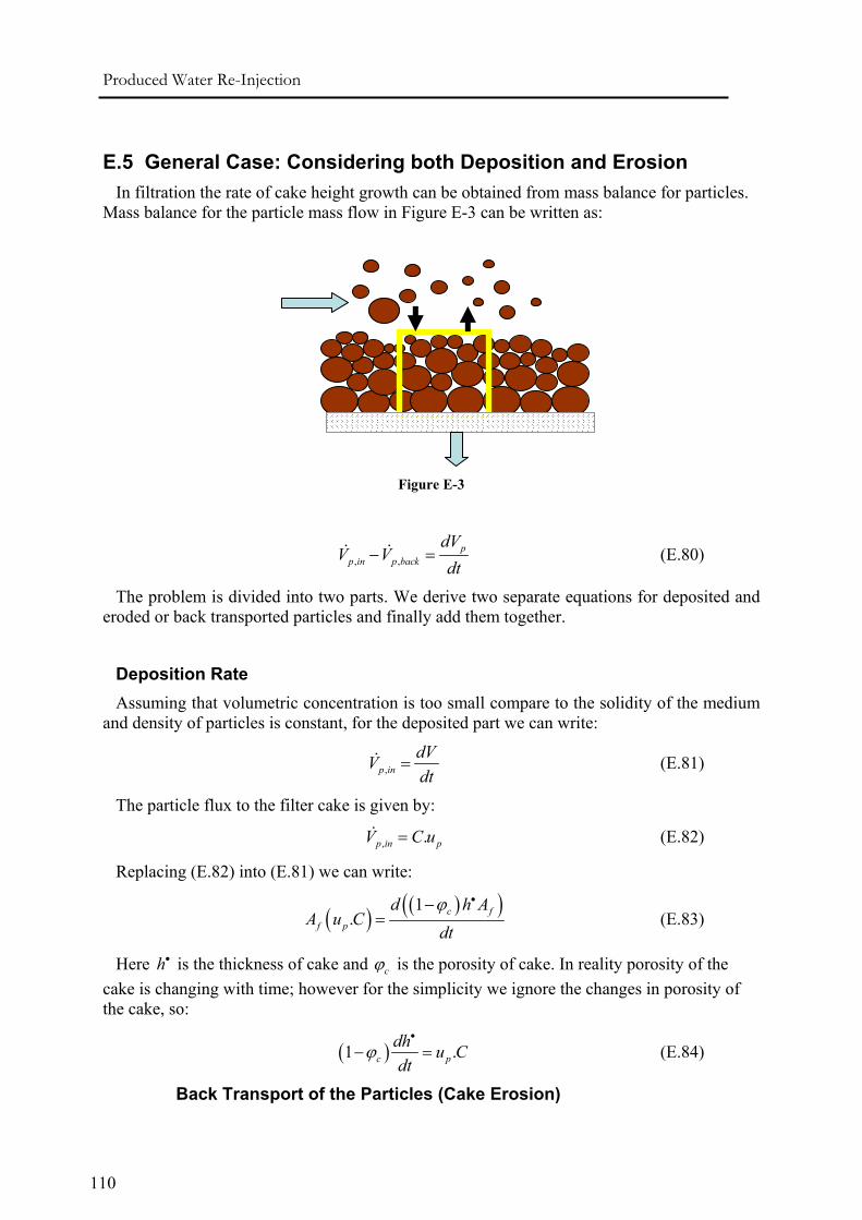
Produced Water Re-Injection
110
E.5 General Case: Considering both Deposition and Erosion In filtration the rate of cake height growth can be obtained from mass balance for particles.
Mass balance for the particle mass flow in Figure E-3 can be written as:
Figure E-3
, ,p
p in p back
dVV V
dt− = (E.80)
The problem is divided into two parts. We derive two separate equations for deposited and eroded or back transported particles and finally add them together.
Deposition Rate Assuming that volumetric concentration is too small compare to the solidity of the medium
and density of particles is constant, for the deposited part we can write:
,p indVVdt
= (E.81)
The particle flux to the filter cake is given by:
, .p in pV C u= (E.82)
Replacing (E.82) into (E.81) we can write:
( ) ( )( )1. c f
f p
d h AA u C
dtϕ •−
= (E.83)
Here h• is the thickness of cake and cϕ is the porosity of cake. In reality porosity of the cake is changing with time; however for the simplicity we ignore the changes in porosity of the cake, so:
( )1 .c pdh u Cdt
ϕ•
− = (E.84)
Back Transport of the Particles (Cake Erosion)
APPENDIX E
111
*
,p backdVVdt
= − (E.85)
The main parameter which causes the back transport of the particles into the system is crossflow velocity [].
.back cfCu uω= (E.86)
α may be called erosion coefficient and will be calculated later.
Again with the same assumptions for back transport or erosion rate we get:
( )*
1 .c cfdh udt
ϕ ω− = (E.87)
Here, *h is the eroded height of the cake and cϕ is the porosity of cake.
Finally if we add (E.84) to (E.87) it follows that:
( ) ( )*
1 . .c p cf
d h hC u u
dtϕ ω
•⎡ ⎤−⎢ ⎥− = −⎢ ⎥⎣ ⎦
(E.88)
Actual height of the cake is the difference between two heights:
*h h h•= − (E.89)
( )1 . .c p cfdh C u udt
ϕ ω− = − (E.90)
Calculation of Erosion Coefficient When cake reaches to equilibrium the rate of deposition and erosion is equal. It means that
the left hand side of (E.88) is zero and as a result α can be calculated by following equation:
p
cf SS
u Cu
ω⎛ ⎞
= ⎜ ⎟⎜ ⎟⎝ ⎠
(E.91)
and for erosion rate we can write:
pback cf
cf SS
u Cm u
u⎛ ⎞
= ⎜ ⎟⎜ ⎟⎝ ⎠
(E.92)
Putting (E.91) into (E.90) the rate of cake growth will be given by:
( )1 . pc p cf
cf SS
u Cdh C u udt u
ϕ⎛ ⎞
− = + ⎜ ⎟⎜ ⎟⎝ ⎠
(E.93)
Or,
( ) ( ) ( )1
6c
SS
dh a C Cdt H h H h
ϕγ
⎡ ⎤⎛ ⎞ ⎛ ⎞− = +⎢ ⎥⎜ ⎟ ⎜ ⎟⎜ ⎟ ⎜ ⎟− −⎢ ⎥⎝ ⎠ ⎝ ⎠⎣ ⎦
(E.94)
Produced Water Re-Injection
112
E.6 Mass Balance Equations for Suspension (With Erosion) To write mass balance equations we divide the control volume into two parts, suspension
and cake. We write mass balance for each part and then add them together to get the equations.
Mass Balance Equation for fluid Part I in the suspension
( )( ) ( )( ) ( )( ),1 ,2
2fp p
cf f cf f fin outincake
H h xWu uu H h W u H h W xW
tρ
ρ ρ ρ∂ − ∆+⎛ ⎞
− = − + ∆ +⎜ ⎟ ∂⎝ ⎠ (E.95)
Part II on the cake
,1 ,2 ,1 ,2
2 2f cp p p p
f fincake outcake
h xWu u u uxW xW
tρ ϕ
ρ ρ⎡ ⎤∂ ∆+ +⎛ ⎞ ⎛ ⎞ ⎣ ⎦∆ = ∆ +⎜ ⎟ ⎜ ⎟ ∂⎝ ⎠ ⎝ ⎠
(E.96)
Assuming that fluid is incompressible and repeating the same procedure as we did for steady state case and replacing (E.96) into (E.95) follows:
( ) ( )1cf c
p
u H h H hu
x tϕ⎡ ⎤∂ − ∂ − −⎡ ⎤⎣ ⎦ ⎣ ⎦− = +
∂ ∂ (E.97)
Mass Balance Equation for Particles Part I in the suspension
( )( ) ( )
( )( ) ( )( ),1 ,2 ,1 ,2
2 2
cf p cf pin
p pp p p pcf p pout
u C H h W u xW
C H h xWC C u uu C H h W xW
t
ρ ω ρ
ρ ρρ ρ
− + ∆ =
∂ − ∆+ +⎛ ⎞− + ∆ +⎜ ⎟ ∂⎝ ⎠
(E.98)
Part II on the cake
( ) ( ),1 ,2 ,1 ,2 12 2
p cp p p pp cf p
h xWC C u uxW u xW
tρ ϕ
ρ ω ρ⎡ ⎤∂ − ∆+ +⎛ ⎞ ⎣ ⎦∆ = ∆ +⎜ ⎟ ∂⎝ ⎠
(E.99)
Assuming that particles are incompressible and replacing (E.99) into (E.98) we will get:
( )( ) ( )( ) ( )( ) ( )1cf cf cin out
u C H h u C H h hC H hx t t
ϕ− − − ∂ −∂ − ⎡ ⎤⎣ ⎦= +∆ ∂ ∂
(E.100)
( ) ( ) ( )1cf cCu H h H h C hx t
ϕ⎡ ⎤∂ − ∂ − + −⎡ ⎤⎣ ⎦ ⎣ ⎦− =∂ ∂
(E.101)
Or:
( )( ) ( ) ( ) ( )1cf c
cf
u H h H h C hCC u H hx x t
ϕ∂ − ∂ − + −⎡ ⎤∂ ⎣ ⎦− − − =∂ ∂ ∂
(E.102)
APPENDIX E
113
Re-arranging of (E.102) follows:
( ) ( ) ( ). 1cf cC hH h C u H h Ct x t
ϕ∂ ∂ ∂⎡ ⎤⎡ ⎤− = − − + − −⎣ ⎦⎢ ⎥∂ ∂ ∂⎣ ⎦ (E.103)

Produced Water Re-Injection
114
115
Appendix F
SATURATION PROCEDURE
Figure , depicts the saturation unit which is used at the beginning of each experiment to saturate the core. Once that is done successfully this unit is disengaged from the experimental setup.
Figure F-1: Schematic of the Saturation Unit (Al-Abduwani, internal report 2003)
F.1 Pre-Saturation Preparation of the Setup
Before attempting to saturate the core, the following steps have to be carried out.
1. Thorough clean up of the core holder 2. Thorough drying of the core holder and the attached pipes 3. Insertion of the core with the appropriate end pieces 4. Ensure that all valves are set to the closed position and then connect the
relevant pipes 5. Pump the confining oil into the annulus and elevate the pressure to the
predetermined confining pressure
Y X
JH
Vacuum
Pump L M
To Core Outlet To Core Inlet
K
Tank 1 Tank 2
N
Produced Water Re-Injection
116
Thorough cleaning of the core holder involves washing the annulus with ethanol. Thus, washing out the remaining oil film that is coating the exterior of the rubber sleeve as well as the interior of the stainless steel core holder. This is done to ensure that no contamination of the core takes place when it is inserted into the rubber sleeve at a later stage.
Once the annular space has been cleaned up, the interior of the rubber sleeve is to be cleaned with a new batch of ethanol. This is done to remove any sand grains or injected particles from the interior of the rubber sleeve. Ensure that the pressure taps are thoroughly cleaned too.
Using pressurised air, the core holder is to be dried. Similarly the accessible pipes should be cleaned and dried.
(Note that the pipes should have been flushed at the end of the previous experiment as part of the post experiment clean-up. If that was not done, then ensure that you read that section and follow the relevant instructions before commencing)
The core and the core plugs should be inserted into the rubber sleeve. The two end caps of the core holder should be firmly sealed. The core holder can now be placed into the setup and oil should be pumped into its annulus. The pressure is to be elevated to the preset value.
The setup is now ready for the saturation process.
F.2 Saturation Procedure
Before commencing with the saturation of the core, thorough preparation of the setup must have been followed as instructed in the previous section.
The first step is to establish vacuum conditions in the two tanks depicted in Figure as well as the area inside the rubber sleeve. Therefore the tubes connecting the pressure taps to the differential pressure gauges have to be checked for leakages. The pipes have to be clean and dry and sealed at the pressure gauge end.
It is also essential that no flow of water takes place. This can be achieved easily if the pressure in the whole system is dropped evenly without creating any pressure differentials that will induce flow.
The beaker in vacuum chamber labelled [Tan k1] should be filled up with a volume of distilled water that is roughly 5 times the volume of the pore-space (this can easily be calculated) and the tubes connecting the saturation unit to the core. This is to ensure that at no point will there be insufficient amount of water. Place a magnet fish in the beaker, which will be used to stir the water to aid the process of deaeration.
APPENDIX F
117
Connect the saturation unit to the setup and engage valves B1 and C1 (Figure 1). Ensure that valves H and J are open, while valves L and M should be closed (Figure ). Needle valve K should be as dilated as possible.
Engage the vacuum pump and ensure that the pressure drops to around –0.95 gauge bars. Maintain at this pressure for 30 minutes while the magnetic stirrer is switched on and is placed under TANK1.
After this time has elapsed, switch off the magnetic stirrer.
Close valve H.
Open valve L very slightly to allow a pressure differential of 0.05 bars and then close it.
Using needle valve K, regulate the flow of water.
Eventually water will start flowing into [Tank2]. However, this process takes some time (approximately 1.5 hours). At this point the vacuum pump should be switched off, valve H opened up and needle valve K fully dilated. The pressure is now equalised and since [Tank1] and [Tank2] are at the same hydrostatic level no back flow should take place.
Manipulate either valve L or M to slowly increase the pressure of the system to atmospheric pressure.
Close valves A, B and C.
Decouple the saturation unit.
Thus, the saturation process has been completed.
F.3 Deaeration of the set up
Some of the pipes between the pump and the core holder will contain some air. Make sure that there is no air in whole system. To that end remove all the existence air in the set up. The below steps should be followed to do the deairation process:
Step 1: Reduce pressure in both tanks down to -1.0 bars. Leave for 2 hours for the water to be deaerated. ([Tank2] is vacuumed. So when relevant valves (B1 & C1) are open it can suck out the existence air in the set up).
Step 2: Now tanks are both vacuumed. To have flow, pressure at the top and the bottom of sample must be different. Therefore close valve J. Use valve M to increase pressure in [Tank1] by increment of 0.05 bars until steady flow is initiated.
Produced Water Re-Injection
118
Step 3: From the preceding experiments the pressure difference between [Tank1] and [Tank2] must be 0.2 bars. Needless to say, to have flow from bottom to top pressure of [Tank1] should be higher than of [Tank2]. Maintain this pressure difference of 0.2 until about 5 times of pore volume has flowed through the core into [Tank2]. Use valves L and M to increase the pressure in tanks, maintaining a dp of 0.2 bars. Use an incremental of 0.1 bars to do this. Wait about 2 minutes at each interval.
[Tank1] (bar) [Tank2] (bar)-0.8 -1.0 -0.7 -0.9 Wait for 2 minutes -0.6 -0.8 Wait for 2 minutes … …. Wait for 2 minutes 0.0 -0.2 Wait for 2 minutes
Step 4: To run the experiment pressure in valve C should be atmospheric. In the last saturation step pressure in valve C is -0.2 while in B is 0.0 barg. If pressure in valve B is equal to pressure in valve C, due to the hydrostatic head flow would occur and the saturation would be affected. To prevent this affect, connect peristaltic pump in location S. Switch on peristaltic pump.
Step 5: Increase pressure in [Tank2] up to atmospheric.
Step 6: Wait for a few PVs.
Step 7: Close valves C & A2 and engage valve A3 so that air in the set up can go out through the pipe. Close valve A3 when water comes out. (Figure 4)
W
C1
2
U
B 12 X
A 12
Y
T
S
3
W
C1
2
U
B 12 X
A 12
Y
T
S
W
C1
2
U
B 12 X
A 12
Y
T
S
W
C1
2
U
B 12 X
A 12
Y
TW
C1
2
U
B 12 X
A 12
Y
T C1
2C
12
U
B 12 B 12 X
A 12 A 12 A 12
Y
T
S
3
Figure 4: schematic of step 7
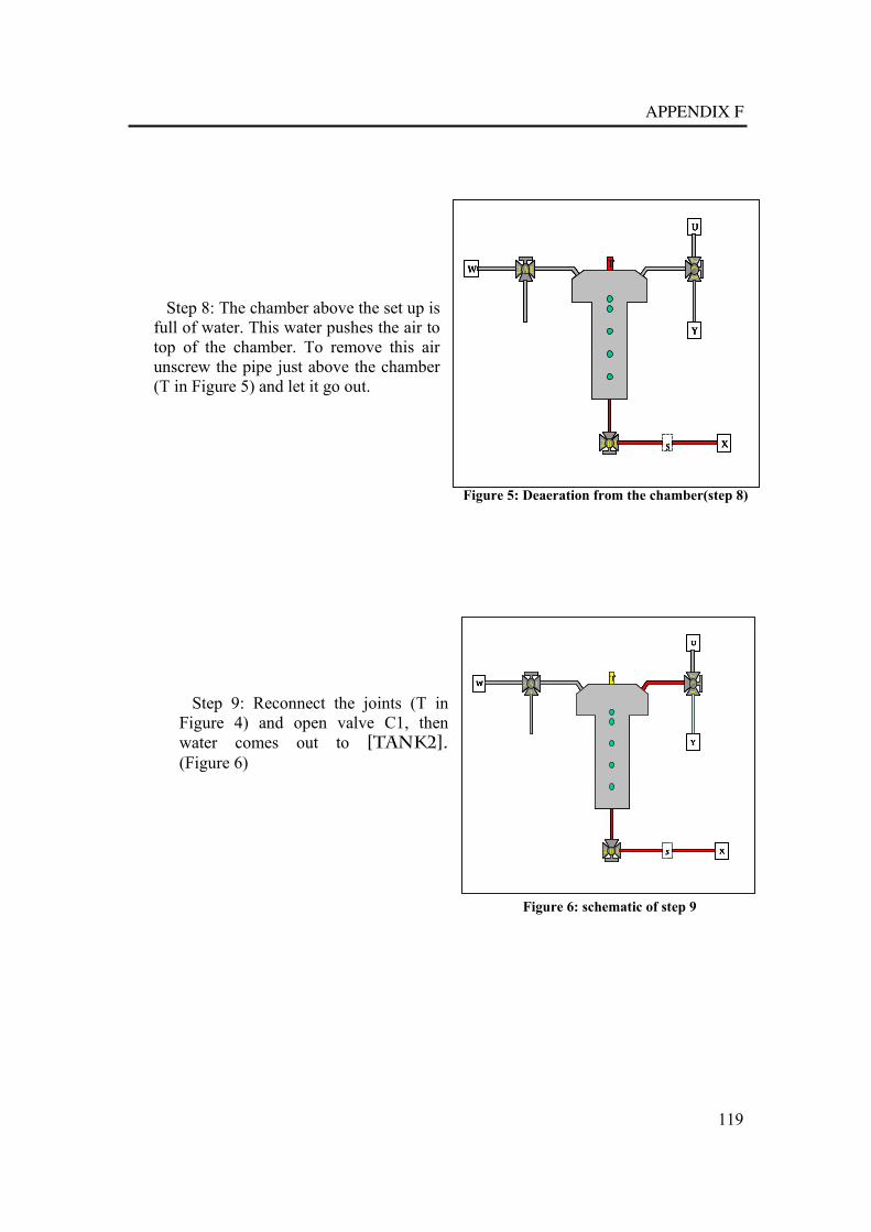
APPENDIX F
119
Step 8: The chamber above the set up is full of water. This water pushes the air to top of the chamber. To remove this air unscrew the pipe just above the chamber (T in Figure 5) and let it go out.
Step 9: Reconnect the joints (T in Figure 4) and open valve C1, then water comes out to [Tank2]. (Figure 6)
W
C1
2
U
B 12 X
A 12
Y
T
S
W
C1
2
U
B 12 X
A 12
Y
T
S
W
C1
2
U
B 12 X
A 12
Y
TW
C1
2
U
B 12 X
A 12
Y
T C1
2C
12
U
B 12 B 12 X
A 12 A 12 A 12
Y
T
S
Figure 5: Deaeration from the chamber(step 8)
W
C1
2
U
B 12 X
A 12
Y
T
S
3W
C1
2
U
B 12 X
A 12
Y
T
S
W
C1
2
U
B 12 X
A 12
Y
T
S
W
C1
2
U
B 12 X
A 12
Y
TW
C1
2
U
B 12 X
A 12
Y
T C1
2C
12
U
B 12 B 12 X
A 12 A 12 A 12
Y
T
S
3
Figure 6: schematic of step 9

Produced Water Re-Injection
120
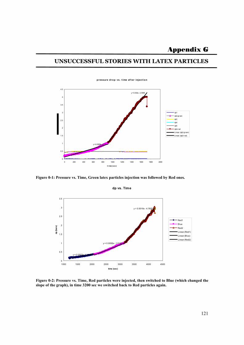
121
Appendix G
UNSUCCESSFUL STORIES WITH LATEX PARTICLES
p ressure d ro p vs. t ime af t er inject io n
y = 0.0009x + 0.12
y = 0.004x - 2.5595
0
0.5
1
1.5
2
2.5
3
3.5
4
4.5
0 200 400 600 800 1000 1200 1400 1600 1800 2000
t i me( sec)
dp1
dp2-gr een
dp3
dp4
dp5
dp2-r ed
Linear (dp2-gr een)
Linear (dp2-r ed)
Figure 0-1: Pressure vs. Time, Green latex particles injection was followed by Red ones.
dp vs. Time
y = 0.0002x - 0.1417
y = 0.0006x - 1.0146
y = 0.0018x - 4.7825
0
0.5
1
1.5
2
2.5
3
3.5
1000 1500 2000 2500 3000 3500 4000 4500
time (sec)
dp (b
ars)
Red1
Blue
Red2
Linear (Red1)
Linear (Blue)
Linear (Red2)
Figure 0-2: Pressure vs. Time, Red particles were injected, then switched to Blue (which changed the slope of the graph), in time 3200 sec we switched back to Red particles again.

Produced Water Re-Injection
123
Appendix H
CAN HEMATITE BE DETECTED USING CT-SCANER?
Sensitivity of equation (6.1) to density difference alone
The following equation will be obtained in this case assuming that: effµ ρ=
1000 . effw
HU ρρ
∆ = ∆ (H.1)
Where after deposition of hematite we will have:
( ) ( )1heff mr h airρ φ ρ ερ φ ε ρ= − + + − (H.2)
ε is the volume of deposited hematite particle over the total volume.
0ε = when there is no deposition. Therefore,
( )0h mreff eff eff h air
h
ρρ ρ ρ ε ρ ρρ
′∆ = − = − (H.3)
where, Mass of hematite
Mass of matrix rockε ′ =
From the previous experiments the amount of deposited hematite is: 0.01ε ′ = . Also using
35400mrkgm
ρ = for hematite we will get:
26.5HU∆ =
Which is higher than minimum measurable value of the Ct-scanner (=10).
Sensitivity to atomic number alone
In this case:
3.8. eZµ β= (H.4) and
3.8
3.81000 e
w
ZHUZ
⎛ ⎞∆∆ = ⎜ ⎟
⎝ ⎠ (H.5)
For the system of hematite and sandstone ( 2SiO ) effective atomic number can be calculated by:
( )3.8 3.8 3.8 3.8. . . .e Si Si Fe Fe O O N NZ g Z g Z g Z g Z= + + + (H.6)
or:
Produced Water Re-Injection
124
1
3.83.8 3.8 3.8 3.8. . . .Si Si Si Si O O N Ne Si Si O N
N Z N Z N Z N ZZ Z Z Z ZG G G G
⎛ ⎞= + + +⎜ ⎟⎝ ⎠
(H.7)
where,
Si Si Fe Fe O O N NG N Z N Z N Z N Z= + + + (H.8)
with,
ii
i
MNζ
= (H.9)
iN is the corresponding number of atom i and
ii
i
mMζ
=
im is the mass of constituent i and iζ is the molecular mass of constituent i .
For a system of sandstone and hematite porosity of sand can be calculated as:
h air
mr h air
V VV V V
φ +=
+ + (H.10)
h
mr
mm
ε ′ = (H.11)
where, mrV is the volume of sand matrix. The mass of corresponding hematite to the chosen arbitrary matrix rock mass is:
.h mrm mε ′= (H.12)
The mass of corresponding air in the chosen control volume can be calculated by:
.h mrh
h h
m mV ερ ρ
′= =
( )mr h air h airV V V V Vφ + + = +
( ) ( )1 1air h mrV V Vφ φ φ− = − +
( )( )
11
mr hair
V VV
φ φφ
− −=
−
therefore,
1air mr hV V Vφ
φ= −
− (H.13)
Using above equations the following equations are obtained to calculate the mass of matrix, air and hematite:
mrm chosen= (H.14)
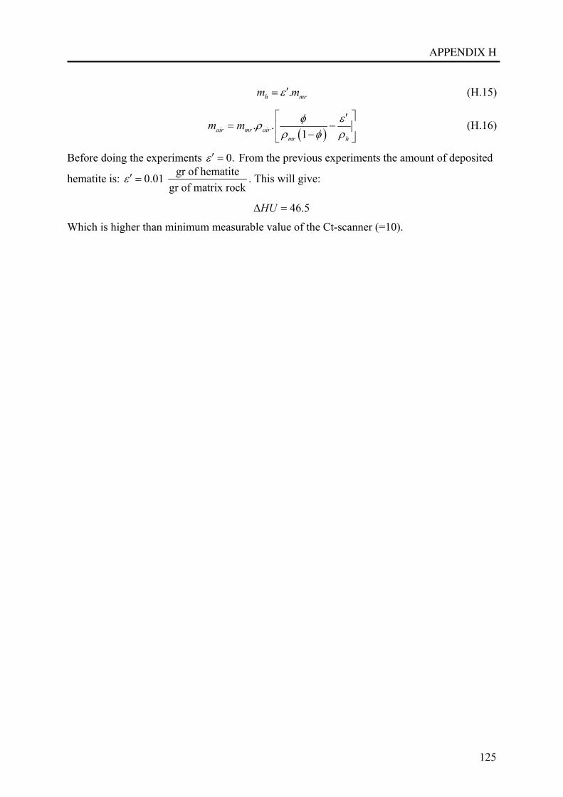
APPENDIX H
125
.h mrm mε ′= (H.15)
( )
. .1air mr air
mr h
m m φ ερρ φ ρ⎡ ⎤′
= −⎢ ⎥−⎣ ⎦ (H.16)
Before doing the experiments 0.ε ′ = From the previous experiments the amount of deposited
hematite is: gr of hematite0.01 gr of matrix rock
ε ′ = . This will give:
46.5HU∆ =
Which is higher than minimum measurable value of the Ct-scanner (=10).

Produced Water Re-Injection
126
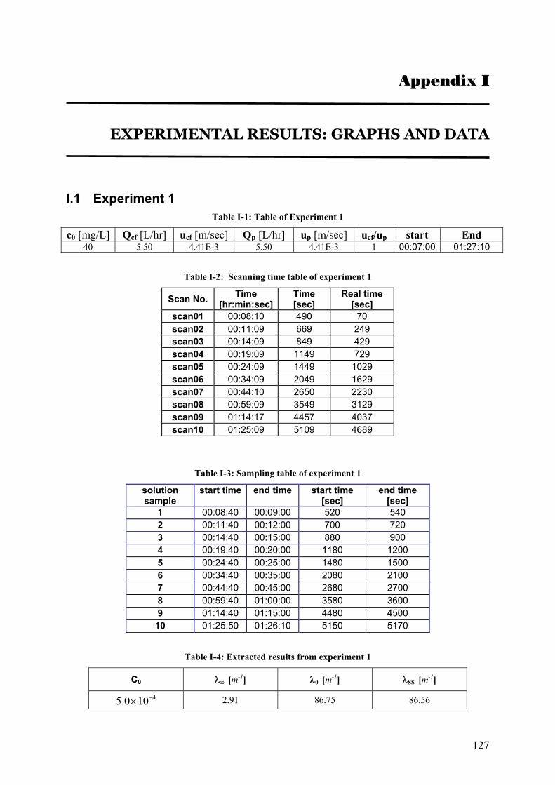
127
Appendix I
I EXPERIMENTAL RESULTS: GRAPHS AND DATA
I.1 Experiment 1 Table I-1: Table of Experiment 1
c0 [mg/L] Qcf [L/hr] ucf [m/sec] Qp [L/hr] up [m/sec] ucf/up start End 40 5.50 4.41E-3 5.50 4.41E-3 1 00:07:00 01:27:10
Table I-2: Scanning time table of experiment 1
Scan No. Time [hr:min:sec]
Time [sec]
Real time [sec]
scan01 00:08:10 490 70 scan02 00:11:09 669 249 scan03 00:14:09 849 429 scan04 00:19:09 1149 729 scan05 00:24:09 1449 1029 scan06 00:34:09 2049 1629 scan07 00:44:10 2650 2230 scan08 00:59:09 3549 3129 scan09 01:14:17 4457 4037 scan10 01:25:09 5109 4689
Table I-3: Sampling table of experiment 1
solution sample
start time end time start time [sec]
end time [sec]
1 00:08:40 00:09:00 520 540 2 00:11:40 00:12:00 700 720 3 00:14:40 00:15:00 880 900 4 00:19:40 00:20:00 1180 1200 5 00:24:40 00:25:00 1480 1500 6 00:34:40 00:35:00 2080 2100 7 00:44:40 00:45:00 2680 2700 8 00:59:40 01:00:00 3580 3600 9 01:14:40 01:15:00 4480 4500
10 01:25:50 01:26:10 5150 5170
Table I-4: Extracted results from experiment 1
C0 λ∞ [m-1] λ0 [m-1] λSS [m-1]
45.0 10−× 2.91 86.75 86.56
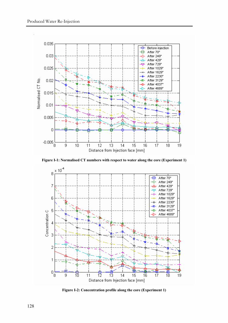
Produced Water Re-Injection
128
Figure I-1: Normalised CT numbers with respect to water along the core (Experiment 1)
Figure I-2: Concentration profile along the core (Experiment 1)
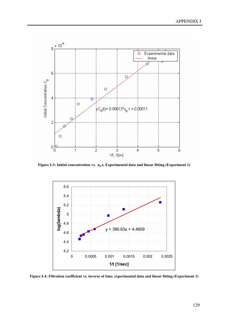
APPENDIX I
129
Figure I-3: Initial concentration vs. up.t, Experimental data and linear fitting (Experiment 1)
y = 390.63x + 4.4609
4.2
4.4
4.6
4.8
5
5.2
5.4
5.6
0 0.0005 0.001 0.0015 0.002 0.0025
1/t [1/sec]
log(
lam
bda)
Figure I-4: Filtration coefficient vs. inverse of time, experimental data and linear fitting (Experiment 1)
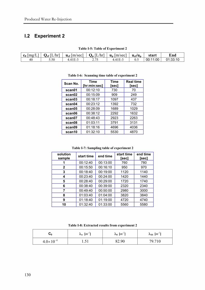
Produced Water Re-Injection
130
I.2 Experiment 2
Table I-5: Table of Experiment 2
c0 [mg/L] Qcf [L/hr] ucf [m/sec] Qp [L/hr] up [m/sec] ucf/up start End 40 5.50 4.41E-3 2.75 4.41E-3 0.5 00:11:00 01:33:10
Table I-6: Scanning time table of experiment 2
Scan No. Time [hr:min:sec]
Time [sec]
Real time [sec]
scan01 00:12:10 730 70 scan02 00:15:09 909 249 scan03 00:18:17 1097 437 scan04 00:23:12 1392 732 scan05 00:28:09 1689 1029 scan06 00:38:12 2292 1632 scan07 00:48:43 2923 2263 scan08 01:03:11 3791 3131 scan09 01:18:16 4696 4036 scan10 01:32:10 5530 4870
Table I-7: Sampling table of experiment 2
solution sample start time end time start time
[sec] end time
[sec] 1 00:12:40 00:13:00 760 780 2 00:15:50 00:16:10 950 970 3 00:18:40 00:19:00 1120 1140 4 00:23:40 00:24:00 1420 1440 5 00:28:40 00:29:00 1720 1740 6 00:38:40 00:39:00 2320 2340 7 00:49:40 00:50:00 2980 3000 8 01:03:40 01:04:00 3820 3840 9 01:18:40 01:19:00 4720 4740
10 01:32:40 01:33:00 5560 5580
Table I-8: Extracted results from experiment 2
C0 λ∞ [m-1] λ0 [m-1] λSS [m-1]
44.0 10−× 1.51 82.90 79.710
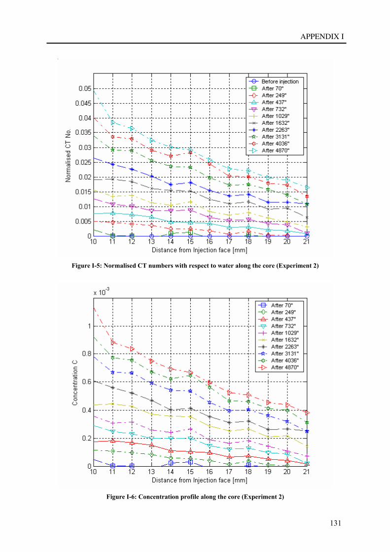
APPENDIX I
131
Figure I-5: Normalised CT numbers with respect to water along the core (Experiment 2)
Figure I-6: Concentration profile along the core (Experiment 2)
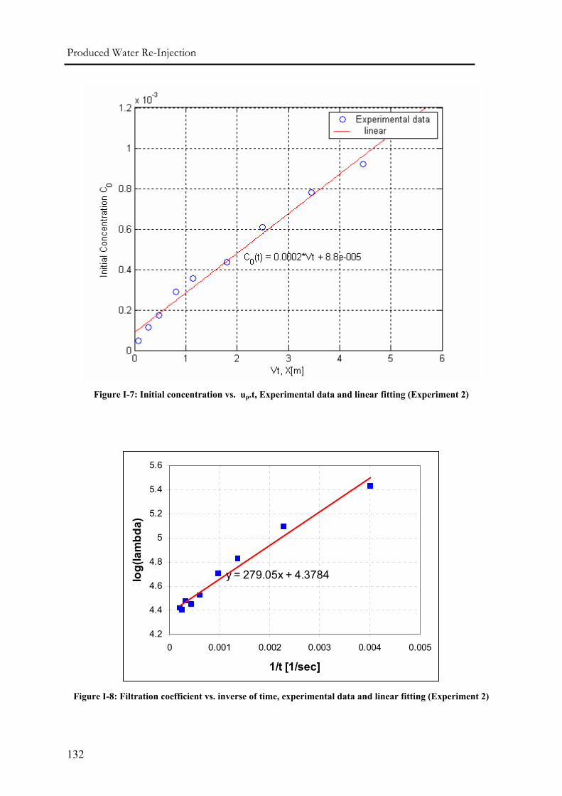
Produced Water Re-Injection
132
Figure I-7: Initial concentration vs. up.t, Experimental data and linear fitting (Experiment 2)
y = 279.05x + 4.3784
4.2
4.4
4.6
4.8
5
5.2
5.4
5.6
0 0.001 0.002 0.003 0.004 0.005
1/t [1/sec]
log(
lam
bda)
Figure I-8: Filtration coefficient vs. inverse of time, experimental data and linear fitting (Experiment 2)
APPENDIX I
133
I.3 Experiment 3
Table I-9: Table of Experiment 3
c0 [mg/L] Qcf [L/hr] ucf [m/sec] Qp [L/hr] up [m/sec] ucf/up start End 30 7.33 5.87E-3 2.75 2.20E-3 0.375 00:08:00 01:12:10
Table I-10: Scanning time table of experiment 3
Scan No. Time [hr:min:sec]
Time [sec]
Real time [sec]
scan01 00:09:10 550 70 scan02 00:12:14 734 254 scan03 00:15:09 909 429 scan04 00:18:10 1090 610 scan05 00:24:09 1449 969 scan06 00:30:19 1819 1339 scan07 00:40:10 2410 1930 scan08 00:50:10 3010 2530 scan09 01:00:09 3609 3129 scan10 01:10:09 4209 3729
Table I-11: Sampling table of experiment 3
solution sample start time end time start time
[sec] end time
[sec] 1 00:09:50 00:10:10 590 610 2 00:12:40 00:13:00 760 780 3 00:15:40 00:16:00 940 960 4 00:18:40 00:19:00 1120 1140 5 00:24:40 00:25:00 1480 1500 6 00:30:40 00:31:00 1840 1860 7 00:40:40 00:41:00 2440 2460 8 00:50:40 00:51:00 3040 3060 9 01:00:40 01:01:00 3640 3660
10 01:10:40 01:11:00 4240 4260
Table I-12: Extracted results from experiment 3
C0 λ∞ [m-1] λ0 [m-1] λSS [m-1]
43.91 10−× 2.08 63.47 58.40
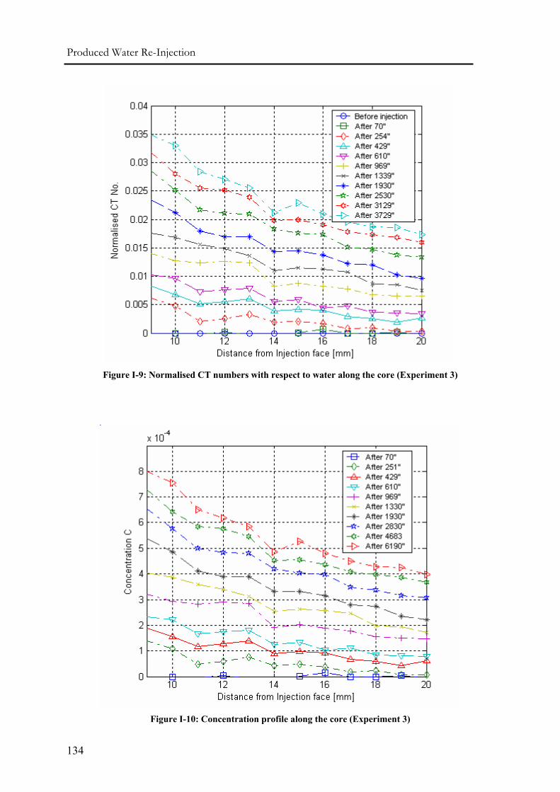
Produced Water Re-Injection
134
Figure I-9: Normalised CT numbers with respect to water along the core (Experiment 3)
Figure I-10: Concentration profile along the core (Experiment 3)
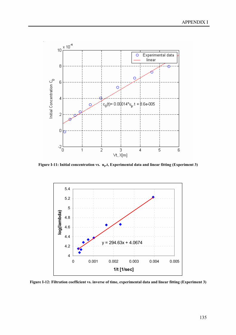
APPENDIX I
135
Figure I-11: Initial concentration vs. up.t, Experimental data and linear fitting (Experiment 3)
y = 294.63x + 4.0674
4
4.2
4.4
4.6
4.8
5
5.2
5.4
0 0.001 0.002 0.003 0.004 0.005
1/t [1/sec]
log(
lam
bda)
Figure I-12: Filtration coefficient vs. inverse of time, experimental data and linear fitting (Experiment 3)
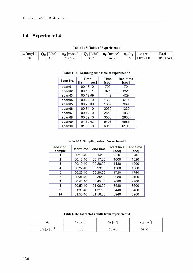
Produced Water Re-Injection
136
I.4 Experiment 4
Table I-13: Table of Experiment 4
c0 [mg/L] Qcf [L/hr] ucf [m/sec] Qp [L/hr] up [m/sec] ucf/up start End 30 7.33 5.87E-3 3.67 2.94E-3 0.5 00:12:00 01:56:40
Table I-14: Scanning time table of experiment 3
Scan No. Time [hr:min:sec]
Time [sec]
Real time [sec]
scan01 00:13:10 790 70 scan02 00:16:11 971 251 scan03 00:19:09 1149 429 scan04 00:22:10 1330 610 scan05 00:28:09 1689 969 scan06 00:34:10 2050 1330 scan07 00:44:10 2650 1930 scan08 00:59:10 3550 2830 scan09 01:30:03 5403 4683 scan10 01:55:10 6910 6190
Table I-15: Sampling table of experiment 4
solution sample start time end time start time
[sec] end time
[sec] 1 00:13:40 00:14:00 820 840 2 00:16:40 00:17:00 1000 1020 3 00:19:40 00:20:00 1180 1200 4 00:22:40 00:23:00 1360 1380 5 00:28:40 00:29:00 1720 1740 6 00:34:40 00:35:00 2080 2100 7 00:44:40 00:45:00 2680 2700 8 00:59:40 01:00:00 3580 3600 9 01:30:40 01:31:00 5440 5460
10 01:55:40 01:56:00 6940 6960
Table I-16: Extracted results from experiment 4
C0 λ∞ [m-1] λ0 [m-1] λSS [m-1]
45.91 10−× 1.18 58.46 54.795
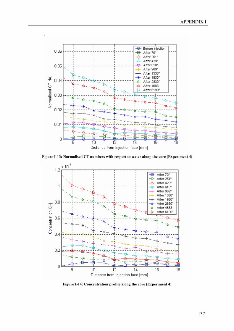
APPENDIX I
137
Figure I-13: Normalised CT numbers with respect to water along the core (Experiment 4)
Figure I-14: Concentration profile along the core (Experiment 4)
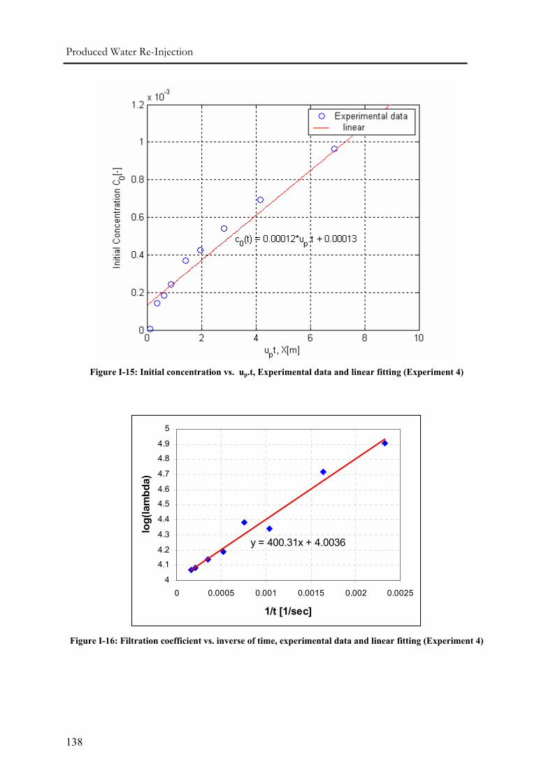
Produced Water Re-Injection
138
Figure I-15: Initial concentration vs. up.t, Experimental data and linear fitting (Experiment 4)
y = 400.31x + 4.0036
4
4.1
4.2
4.3
4.4
4.5
4.6
4.7
4.8
4.9
5
0 0.0005 0.001 0.0015 0.002 0.0025
1/t [1/sec]
log(
lam
bda)
Figure I-16: Filtration coefficient vs. inverse of time, experimental data and linear fitting (Experiment 4)
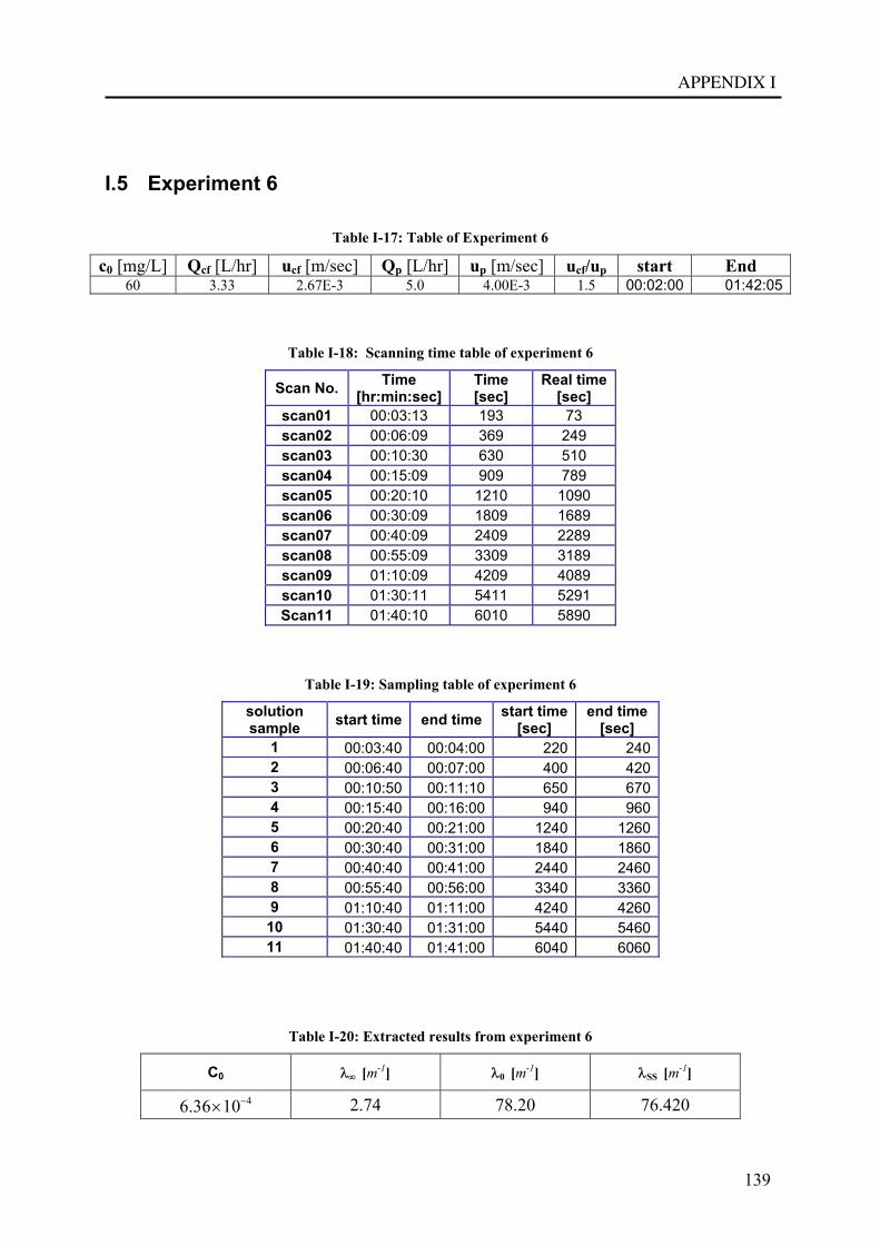
APPENDIX I
139
I.5 Experiment 6
Table I-17: Table of Experiment 6
c0 [mg/L] Qcf [L/hr] ucf [m/sec] Qp [L/hr] up [m/sec] ucf/up start End 60 3.33 2.67E-3 5.0 4.00E-3 1.5 00:02:00 01:42:05
Table I-18: Scanning time table of experiment 6
Scan No. Time [hr:min:sec]
Time [sec]
Real time [sec]
scan01 00:03:13 193 73 scan02 00:06:09 369 249 scan03 00:10:30 630 510 scan04 00:15:09 909 789 scan05 00:20:10 1210 1090 scan06 00:30:09 1809 1689 scan07 00:40:09 2409 2289 scan08 00:55:09 3309 3189 scan09 01:10:09 4209 4089 scan10 01:30:11 5411 5291 Scan11 01:40:10 6010 5890
Table I-19: Sampling table of experiment 6
solution sample start time end time start time
[sec] end time
[sec] 1 00:03:40 00:04:00 220 240 2 00:06:40 00:07:00 400 420 3 00:10:50 00:11:10 650 670 4 00:15:40 00:16:00 940 960 5 00:20:40 00:21:00 1240 1260 6 00:30:40 00:31:00 1840 1860 7 00:40:40 00:41:00 2440 2460 8 00:55:40 00:56:00 3340 3360 9 01:10:40 01:11:00 4240 4260
10 01:30:40 01:31:00 5440 5460 11 01:40:40 01:41:00 6040 6060
Table I-20: Extracted results from experiment 6
C0 λ∞ [m-1] λ0 [m-1] λSS [m-1]
46.36 10−× 2.74 78.20 76.420
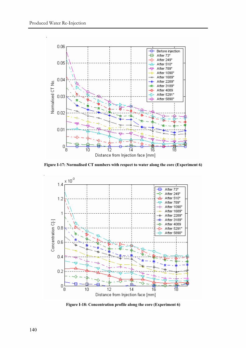
Produced Water Re-Injection
140
Figure I-17: Normalised CT numbers with respect to water along the core (Experiment 6)
Figure I-18: Concentration profile along the core (Experiment 6)
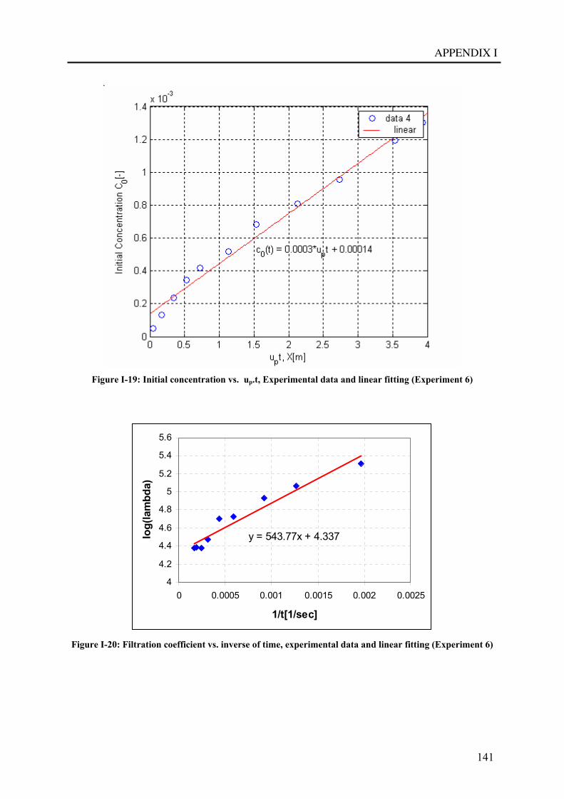
APPENDIX I
141
Figure I-19: Initial concentration vs. up.t, Experimental data and linear fitting (Experiment 6)
y = 543.77x + 4.337
4
4.2
4.4
4.6
4.8
5
5.2
5.4
5.6
0 0.0005 0.001 0.0015 0.002 0.0025
1/t[1/sec]
log(
lam
bda)
Figure I-20: Filtration coefficient vs. inverse of time, experimental data and linear fitting (Experiment 6)
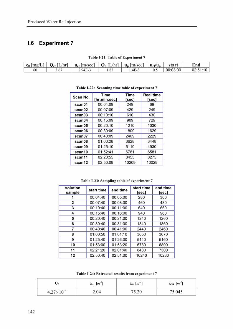
Produced Water Re-Injection
142
I.6 Experiment 7
Table I-21: Table of Experiment 7
c0 [mg/L] Qcf [L/hr] ucf [m/sec] Qp [L/hr] up [m/sec] ucf/up start End 60 3.67 2.94E-3 1.83 1.4E-3 0.5 00:03:00 02:51:10
Table I-22: Scanning time table of experiment 7
Scan No. Time [hr:min:sec]
Time [sec]
Real time [sec]
scan01 00:04:09 249 69 scan02 00:07:09 429 249 scan03 00:10:10 610 430 scan04 00:15:09 909 729 scan05 00:20:10 1210 1030 scan06 00:30:09 1809 1629 scan07 00:40:09 2409 2229 scan08 01:00:28 3628 3448 scan09 01:25:10 5110 4930 scan10 01:52:41 6761 6581 scan11 02:20:55 8455 8275 scan12 02:50:09 10209 10029
Table I-23: Sampling table of experiment 7
solution sample start time end time start time
[sec] end time
[sec] 1 00:04:40 00:05:00 280 300 2 00:07:40 00:08:00 460 480 3 00:10:40 00:11:00 640 660 4 00:15:40 00:16:00 940 960 5 00:20:40 00:21:00 1240 1260 6 00:30:40 00:31:00 1840 1860 7 00:40:40 00:41:00 2440 2460 8 01:00:50 01:01:10 3650 3670 9 01:25:40 01:26:00 5140 5160
10 01:53:00 01:53:20 6780 6800 11 02:21:20 02:01:40 8480 7300 12 02:50:40 02:51:00 10240 10260
Table I-24: Extracted results from experiment 7
C0 λ∞ [m-1] λ0 [m-1] λSS [m-1]
44.27 10−× 2.04 75.20 75.045
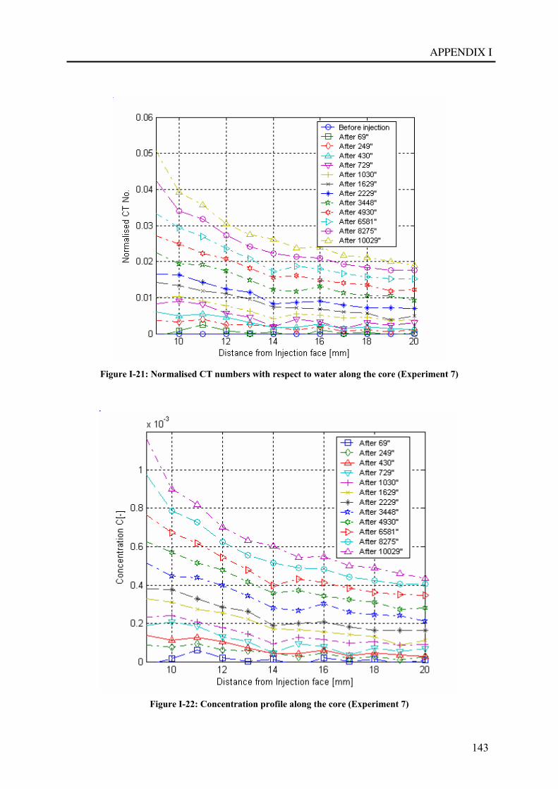
APPENDIX I
143
Figure I-21: Normalised CT numbers with respect to water along the core (Experiment 7)
Figure I-22: Concentration profile along the core (Experiment 7)
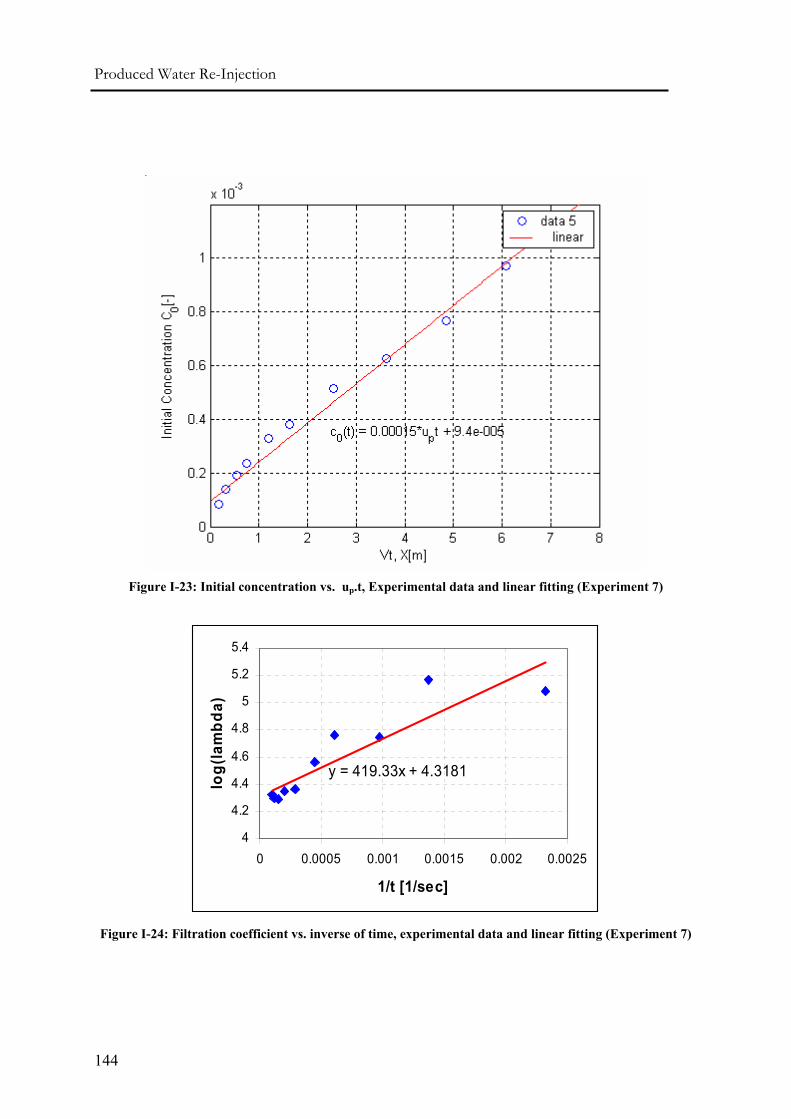
Produced Water Re-Injection
144
Figure I-23: Initial concentration vs. up.t, Experimental data and linear fitting (Experiment 7)
y = 419.33x + 4.3181
4
4.2
4.4
4.6
4.8
5
5.2
5.4
0 0.0005 0.001 0.0015 0.002 0.0025
1/t [1/sec]
log(
lam
bda)
Figure I-24: Filtration coefficient vs. inverse of time, experimental data and linear fitting (Experiment 7)
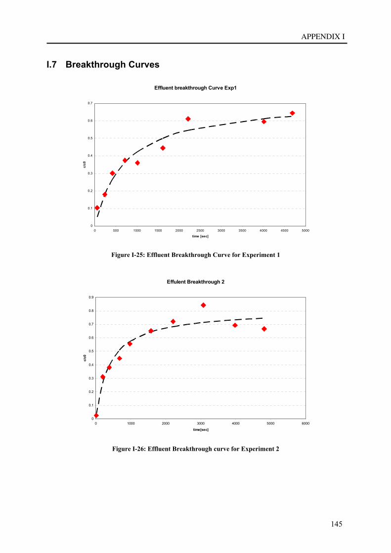
APPENDIX I
145
I.7 Breakthrough Curves
Effluent breakthrough Curve Exp1
0
0.1
0.2
0.3
0.4
0.5
0.6
0.7
0 500 1000 1500 2000 2500 3000 3500 4000 4500 5000
time [sec]
c/c0
Figure I-25: Effluent Breakthrough Curve for Experiment 1
Effulent Breakthrough 2
0
0.1
0.2
0.3
0.4
0.5
0.6
0.7
0.8
0.9
0 1000 2000 3000 4000 5000 6000
time[sec]
c/c0
Figure I-26: Effluent Breakthrough curve for Experiment 2
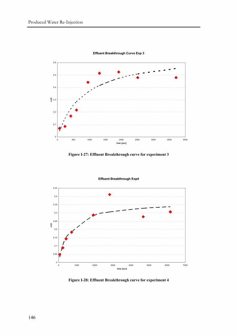
Produced Water Re-Injection
146
Effluent Breakthrough Curve Exp 3
0
0.1
0.2
0.3
0.4
0.5
0.6
0 500 1000 1500 2000 2500 3000 3500 4000
time [sec]
c/c0
Figure I-27: Effluent Breakthrough curve for experiment 3
Effluent Breakthrough Exp4
0
0.05
0.1
0.15
0.2
0.25
0.3
0.35
0.4
0.45
0 1000 2000 3000 4000 5000 6000 7000
time [sec]
c/c0
Figure I-28: Effluent Breakthrough curve for experiment 4

APPENDIX I
147
Effluent Breakthrough Curve-Exp5
0
0.1
0.2
0.3
0.4
0.5
0.6
0 500 1000 1500 2000 2500 3000 3500 4000 4500
Time (sec)
c/c0
Figure I-29: Effluent breakthrough curve for experiment 5
I.8 Permeability Decline Curves
Exp1
0
0.2
0.4
0.6
0.8
1
1.2
0 1000 2000 3000 4000 5000 6000
PV
norm
k
Figure I-30: Permeability decline curve for Experiment 1
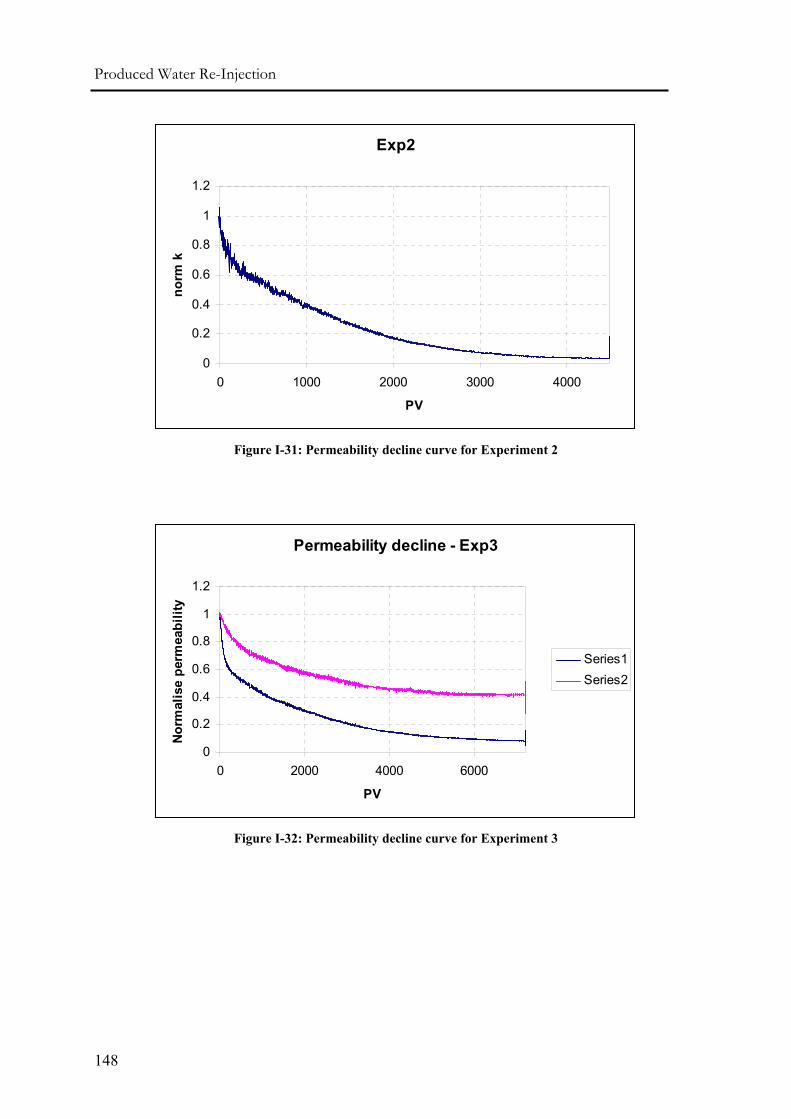
Produced Water Re-Injection
148
Exp2
0
0.2
0.4
0.6
0.8
1
1.2
0 1000 2000 3000 4000
PV
norm
k
Figure I-31: Permeability decline curve for Experiment 2
Permeability decline - Exp3
0
0.2
0.4
0.6
0.8
1
1.2
0 2000 4000 6000
PV
Nor
mal
ise
perm
eabi
lity
Series1Series2
Figure I-32: Permeability decline curve for Experiment 3
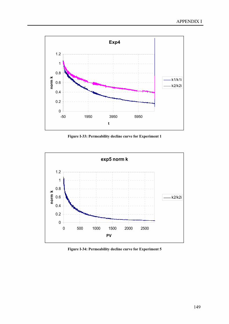
APPENDIX I
149
Exp4
0
0.2
0.4
0.6
0.8
1
1.2
-50 1950 3950 5950
t
norm
k k1/k1ik2/k2i
Figure I-33: Permeability decline curve for Experiment 1
exp5 norm k
0
0.2
0.4
0.6
0.8
1
1.2
0 500 1000 1500 2000 2500
PV
norm
k
k2/k2i
Figure I-34: Permeability decline curve for Experiment 5

Produced Water Re-Injection
150
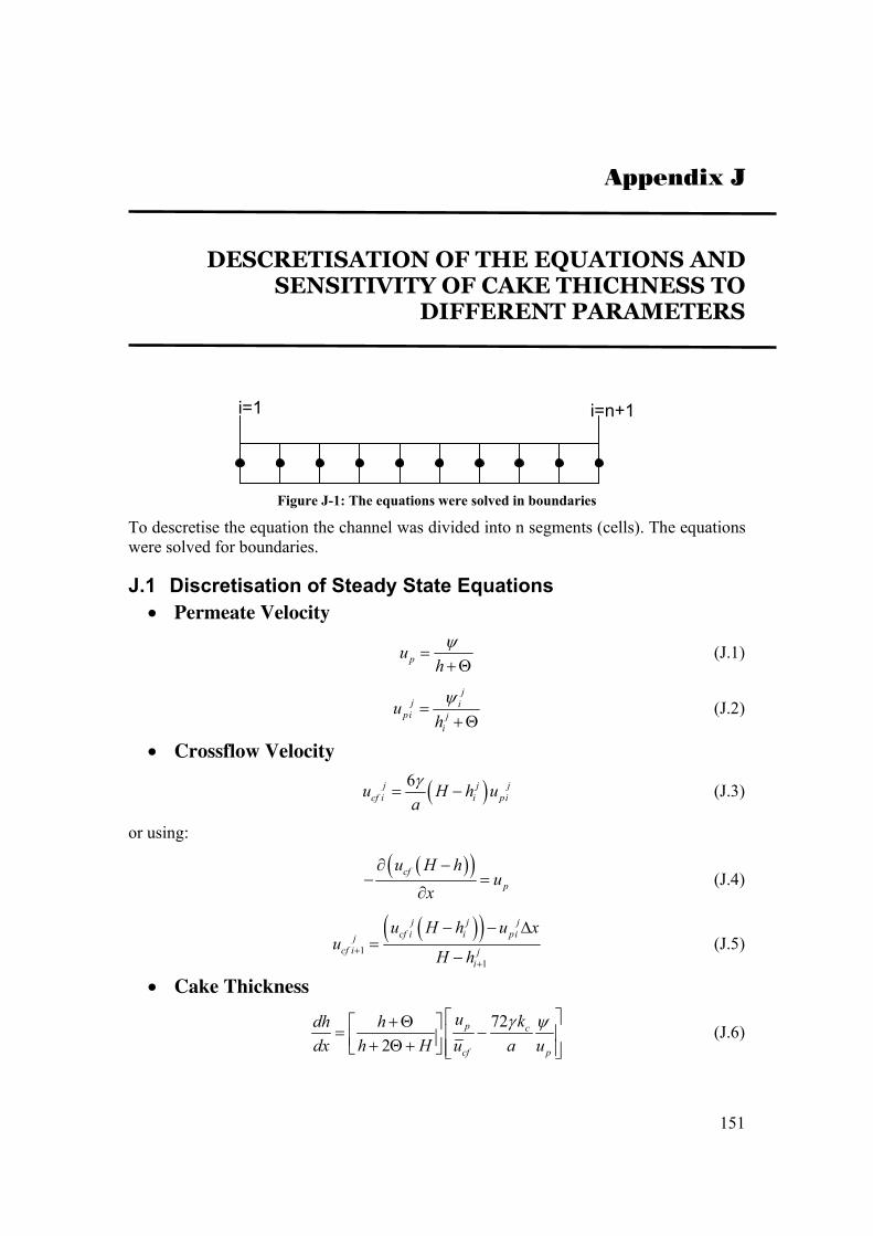
151
Appendix J
J DESCRETISATION OF THE EQUATIONS AND
SENSITIVITY OF CAKE THICHNESS TO DIFFERENT PARAMETERS
Figure J-1: The equations were solved in boundaries
To descretise the equation the channel was divided into n segments (cells). The equations were solved for boundaries.
J.1 Discretisation of Steady State Equations • Permeate Velocity
puhψ
=+Θ
(J.1)
j
j ipi j
i
uhψ
=+Θ
(J.2)
• Crossflow Velocity
( )6j j jcf i i piu H h u
aγ
= − (J.3)
or using:
( )( )cf
p
u H hu
x∂ −
− =∂
(J.4)
( )( )
11
j j jcf i i pij
cf i ji
u H h u xu
H h++
− − ∆=
− (J.5)
• Cake Thickness
722
p c
cf p
u kdh hdx h H u a u
γ ψ⎡ ⎤+Θ⎡ ⎤= −⎢ ⎥⎢ ⎥+ Θ+⎣ ⎦ ⎢ ⎥⎣ ⎦ (J.6)
i=1 i=n+1
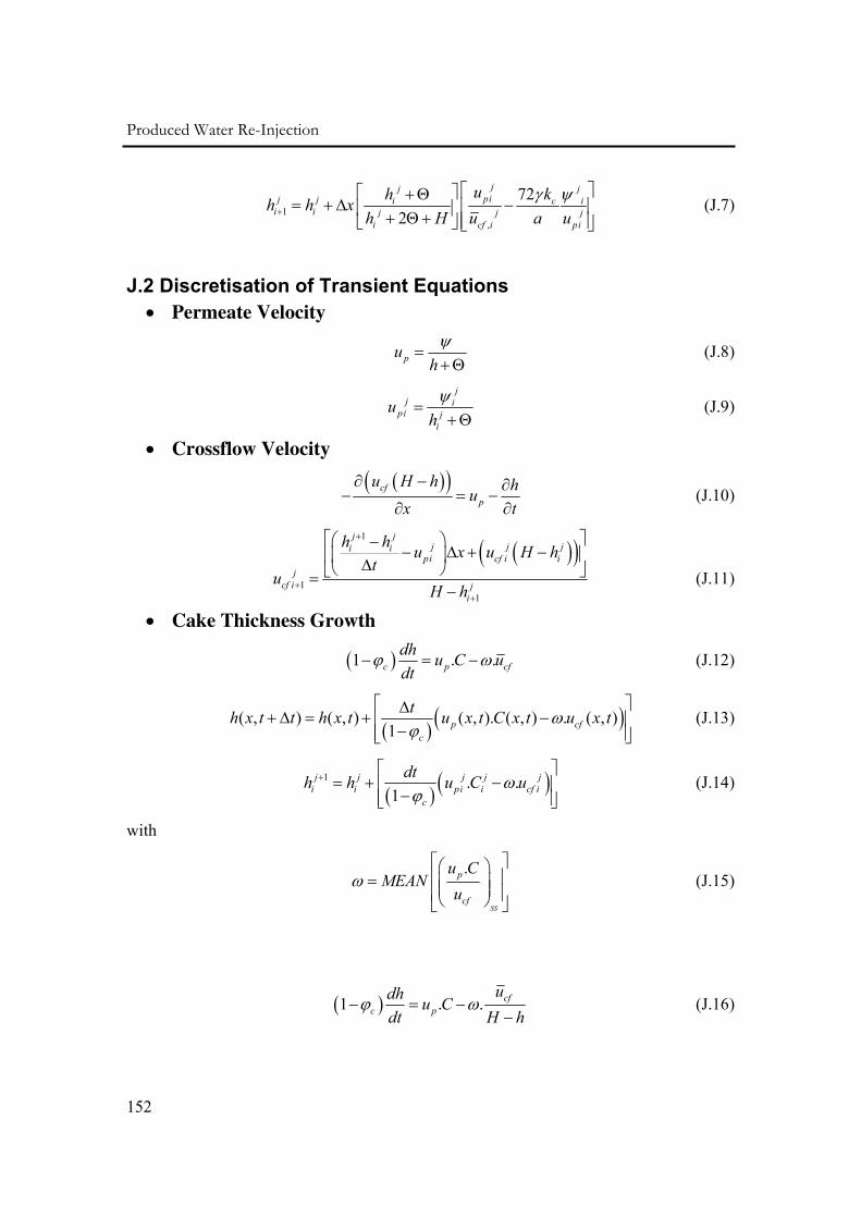
Produced Water Re-Injection
152
1,
722
jj jpij j i c i
i i j j ji cf i pi
uh kh h xh H u a u
γ ψ+
⎡ ⎤⎡ ⎤+Θ= + ∆ −⎢ ⎥⎢ ⎥+ Θ+ ⎢ ⎥⎣ ⎦ ⎣ ⎦
(J.7)
J.2 Discretisation of Transient Equations • Permeate Velocity
puhψ
=+Θ
(J.8)
j
j ipi j
i
uhψ
=+Θ
(J.9)
• Crossflow Velocity
( )( )cf
p
u H h hux t
∂ − ∂− = −
∂ ∂ (J.10)
( )( )
1
11
j jj j ji i
pi cf i ij
cf i ji
h h u x u H ht
uH h
+
++
⎡ ⎤⎛ ⎞−− ∆ + −⎢ ⎥⎜ ⎟∆⎝ ⎠⎣ ⎦=
− (J.11)
• Cake Thickness Growth
( )1 . .c p cfdh u C udt
ϕ ω− = − (J.12)
( ) ( )( , ) ( , ) ( , ). ( , ) . ( , )1 p cf
c
th x t t h x t u x t C x t u x tωϕ
⎡ ⎤∆+ ∆ = + −⎢ ⎥
−⎢ ⎥⎣ ⎦ (J.13)
( ) ( )1 . .1
j j j j ji i pi i cf i
c
dth h u C uωϕ
+ ⎡ ⎤= + −⎢ ⎥
−⎢ ⎥⎣ ⎦ (J.14)
with
.
SS
p
cf
u CMEAN
uω
⎡ ⎤⎛ ⎞⎢ ⎥= ⎜ ⎟⎜ ⎟⎢ ⎥⎝ ⎠⎣ ⎦
(J.15)
( )1 . . cfc p
udh u Cdt H h
ϕ ω− = −−
(J.16)
APPENDIX J
153
( )
( , )( , ) ( , ) ( , ). ( , ) .
1 ( , )cf
pc
u x tth x t t h x t u x t C x tH h x t
ωϕ
⎡ ⎤⎛ ⎞∆+ ∆ = + −⎢ ⎥⎜ ⎟− −⎢ ⎥⎝ ⎠⎣ ⎦
(J.17)
( )
1 . .1
jcf ij j j j
i i pi i jc i
udth h u CH h
ωϕ
+⎡ ⎤⎛ ⎞
= + −⎢ ⎥⎜ ⎟⎜ ⎟− −⎢ ⎥⎝ ⎠⎣ ⎦ (J.18)
With:
.6 SS
a CMEANωγ
⎡ ⎤⎛ ⎞= ⎢ ⎥⎜ ⎟
⎝ ⎠⎣ ⎦ (J.19)
if we assume that the back transport can be written as:
( )
.m
cfback n
uu C
H hω=
− (J.20)
then:
( )( )
1 . .m
cfc p n
udh u Cdt H h
ϕ ω− = −−
(J.21)
and:
( ) 1
1
.6
n
mcf SS
a H h CMEAN
uω
γ
−
−
⎡ ⎤⎛ ⎞−⎢ ⎥⎜ ⎟=⎜ ⎟⎢ ⎥⎝ ⎠⎣ ⎦
(J.22)
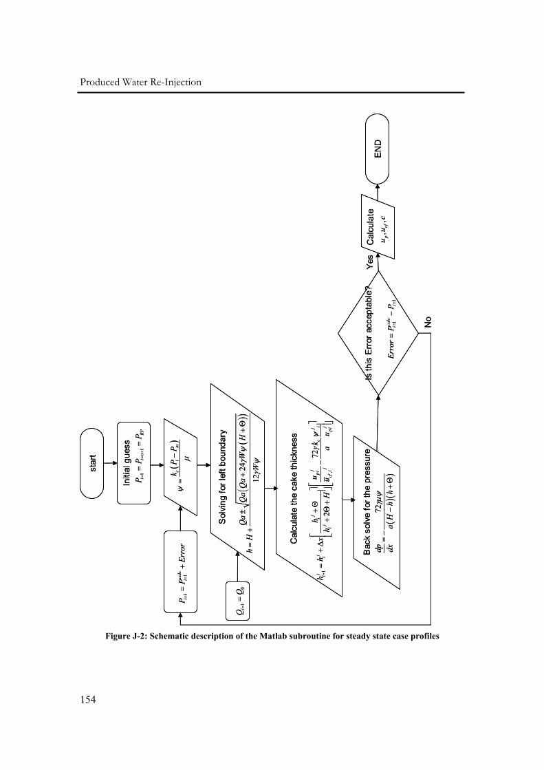
Produced Water Re-Injection
154
Figure J-2: Schematic description of the Matlab subroutine for steady state case profiles
Cal
cula
te th
e ca
ke th
ickn
ess
Sol
ving
for l
eft b
ound
ary
star
t
Initi
al g
uess
11
ii
nBP
PP
P=
=+
==
()
ci
mk
PP
ψµ−
=1
1calc
ii
PP
Erro
r=
==
+
()
()
24
12
Qa
Qa
Qa
WH
hH
W
γψ
γψ
±+
+Θ
=+
10
iQ
Q==
1,
722
jj
jpi
jj
ic
ii
ij
jj
icf
ipi
uh
kh
hx
hH
ua
uγ
ψ+
⎡⎤
⎡⎤
+Θ
=+∆
−⎢
⎥⎢
⎥+
Θ+
⎢⎥
⎣⎦ ⎣
⎦
Bac
k so
lve
for t
he p
ress
ure
()(
)72
dp dxa
Hh
hγµψ
=−
−+Θ
Is th
is E
rror
acc
epta
ble?
11
calc
ii
Erro
rP
P=
==
−
No
Cal
cula
te,
,p
cfu
uc
Yes
EN
D
Cal
cula
te th
e ca
ke th
ickn
ess
Sol
ving
for l
eft b
ound
ary
star
t
Initi
al g
uess
11
ii
nBP
PP
P=
=+
==
()
ci
mk
PP
ψµ−
=1
1calc
ii
PP
Erro
r=
==
+
()
()
24
12
Qa
Qa
Qa
WH
hH
W
γψ
γψ
±+
+Θ
=+
10
iQ
Q==
1,
722
jj
jpi
jj
ic
ii
ij
jj
icf
ipi
uh
kh
hx
hH
ua
uγ
ψ+
⎡⎤
⎡⎤
+Θ
=+∆
−⎢
⎥⎢
⎥+
Θ+
⎢⎥
⎣⎦ ⎣
⎦
Bac
k so
lve
for t
he p
ress
ure
()(
)72
dp dxa
Hh
hγµψ
=−
−+Θ
Is th
is E
rror
acc
epta
ble?
11
calc
ii
Erro
rP
P=
==
−
No
Cal
cula
te,
,p
cfu
uc
Yes
EN
D
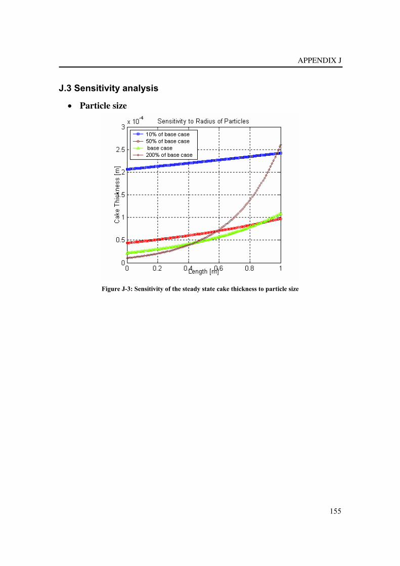
APPENDIX J
155
J.3 Sensitivity analysis
• Particle size
Figure J-3: Sensitivity of the steady state cake thickness to particle size
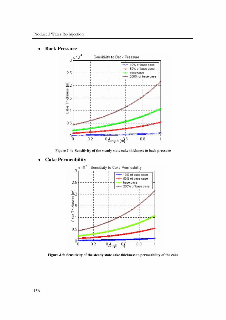
Produced Water Re-Injection
156
• Back Pressure
Figure J-4: Sensitivity of the steady state cake thickness to back pressure
• Cake Permeability
Figure J-5: Sensitivity of the steady state cake thickness to permeability of the cake
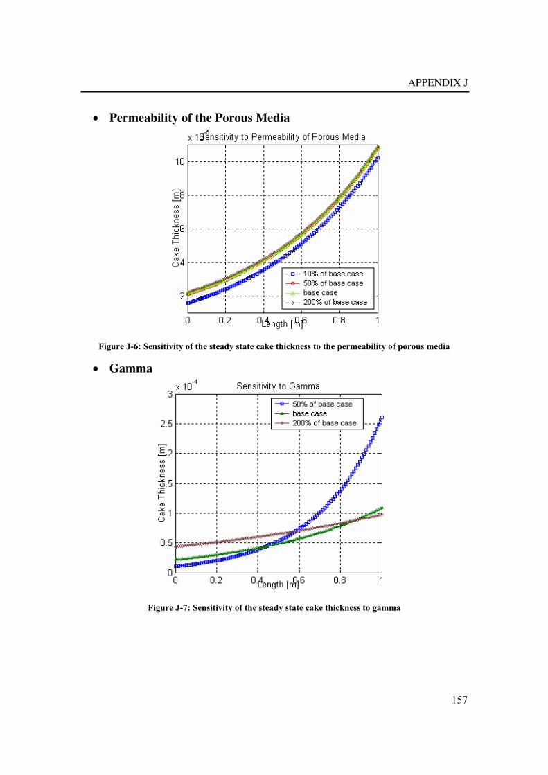
APPENDIX J
157
• Permeability of the Porous Media
Figure J-6: Sensitivity of the steady state cake thickness to the permeability of porous media
• Gamma
Figure J-7: Sensitivity of the steady state cake thickness to gamma

Produced Water Re-Injection
158

159
ACKNOWLEDGMENT I am gratefully thankful for the God who gave me the ability to carry on this work.
I feel very thankful to my home country Iran in which I was raised and educated until my B.Sc. degree. My thanks also go to the Netherlands for giving me the opportunity to do this research.
The most obvious debt is certainly to Peter Currie, Wim van den Broek and Firas Al-Albduwani for their great supervision, support and guidance during the different stages of my work.
I would like to thank NIOC (National Iranian Oil Company) for sponsoring me. PDO (Petroleum Development Oman) is thanked for their contribution to this thesis as are NWO (Netherlands Organisation for Scientific Research).
Special thanks to the people in the Dietz lab. The technical staff Leo Vogt, Adri Maljaars, Peter de Vreede, Karel Heller, Gerard Mathu, Andre Hoving and others for their technical support and valuable advice during my research time. Also my special thanks go to the people in the chemistry laboratory of Applied Earth Science faculty.
I would like to thank my friends Firas Al-Abduwani, Ali Naderi Beni, Alireza Hassanzadegan, Siyavash Motealleh, Bert-Rick de Zwart and Patrick Tardy for their enjoyable company during lunch times and the stimulating Dart tournaments. Special thanks to Hani Soloman for the delectable lunches on Tuesdays.
Last but not least, I thank my lovely mother, honorable father and my kind family for their emotional support and keeping me motivated to carry on this work.
Related Documents